analysis of potential water-supply management options ... · scientific investigations report...
TRANSCRIPT
U.S. Department of the InteriorU.S. Geological Survey
Scientific Investigations Report 2014–5081
Prepared in cooperation with Fort Irwin National Training Center
Analysis of Potential Water-Supply Management Options, 2010–60, and Documentation of Revisions to the Model of the Irwin Basin Aquifer System, Fort Irwin National Training Center, California

Cover. Aerial view of Fort Irwin Military Reservation, Fort Irwin, California. Photo taken by Bobak Ha’Eri, on July 27, 2009.

Analysis of Potential Water-Supply Management Options, 2010–60, and Documentation of Revisions to the Model of the Irwin Basin Aquifer System, Fort Irwin National Training Center, California
By Lois M. Voronin, Jill N. Densmore, and Peter Martin
Prepared in cooperation with Fort Irwin National Training Center
Scientific Investigations Report 2014–5081
U.S. Department of the InteriorU.S. Geological Survey

U.S. Department of the InteriorSALLY JEWELL, Secretary
U.S. Geological SurveySuzette M. Kimball, Acting Director
U.S. Geological Survey, Reston, Virginia: 2014
For more information on the USGS—the Federal source for science about the Earth, its natural and living resources, natural hazards, and the environment, visit http://www.usgs.gov or call 1–888–ASK–USGS.
For an overview of USGS information products, including maps, imagery, and publications, visit http://www.usgs.gov/pubprod
To order this and other USGS information products, visit http://store.usgs.gov
Any use of trade, firm, or product names is for descriptive purposes only and does not imply endorsement by the U.S. Government.
Although this information product, for the most part, is in the public domain, it also may contain copyrighted materials as noted in the text. Permission to reproduce copyrighted items must be secured from the copyright owner.
Suggested citation:Voronin, L.M., Densmore, J.N., and Martin, Peter, 2014, Analysis of potential water-supply management options, 2010–60, and documentation of revisions to the model of the Irwin Basin Aquifer System, Fort Irwin National Training Center, California: U.S. Geological Survey Scientific Investigations Report 2014–5081, 34 p., http://dx.doi.org/10.3133/sir20145081.
ISSN 2328-0328 (online)
iii
Contents
Abstract ..........................................................................................................................................................1Introduction.....................................................................................................................................................1
Purpose and Scope ..............................................................................................................................1Location and Description of Study Area ...........................................................................................2Hydrogeologic Setting .........................................................................................................................2
Simulation of Groundwater Flow .................................................................................................................9Model Design.........................................................................................................................................9Model Calibration................................................................................................................................12Groundwater Withdrawals ................................................................................................................14Groundwater Recharge .....................................................................................................................14
Simulated Effects of Future Withdrawals and Artificial Recharge .....................................................20Description of Model Scenarios ......................................................................................................21
Scenario 1 ...................................................................................................................................21Scenario 2 ...................................................................................................................................22Scenario 3 ...................................................................................................................................24Scenario 4 ...................................................................................................................................24
Results of Simulations ........................................................................................................................24Scenario 1 ...................................................................................................................................24Scenario 2 ...................................................................................................................................31Scenario 3 ...................................................................................................................................31Scenario 4 ...................................................................................................................................31
Model Limitations................................................................................................................................31Summary and Conclusions .........................................................................................................................32References Cited..........................................................................................................................................33

iv
Figures 1. Map showing location of study area at Fort Irwin National
Training Center, California ...........................................................................................................3 2. Generalized map of the Irwin Basin, Fort Irwin National
Training Center, California ...........................................................................................................4 3. Figures showing generalized geology of the Irwin Basin, Fort Irwin
National Training Center, California ...........................................................................................5 4. Figure showing altitude of the basement complex and boundaries
of groundwater model layers for the Irwin Basin, Fort Irwin National Training Center, California ...........................................................................................................8
5. Cross-sectional view of model layers, hydraulic conductivities, and boundary conditions of the Irwin Basin, Fort Irwin National Training Center, California .................10
6. Map showing simulated 1994 hydraulic heads, layer 1, Irwin Basin, Fort Irwin National Training Center, California .........................................................................................13
7. Hydrographs of measured water levels and simulated hydraulic heads in 11 observation wells, Irwin Basin, Fort Irwin National Training Center, California .........................................................................................................15
8. Graph showing annual groundwater recharge and withdrawals from Bicycle, Irwin, and Langford Basins, Fort Irwin National Training Center, California, 1941–2010 ..................................................................................................................16
9. Hydrographs of measured water levels and simulated hydraulic heads in six observation wells near the wastewater-treatment facility, Irwin Basin, Fort Irwin National Training Center, California .........................................................................................20
10. Graph showing average 2001 to 2010 total monthly groundwater withdrawal distribution for wells in the Bicycle, Irwin, and Langford Basins that were used to provide water to Fort Irwin National Training Center, California ........................................21
11. Map showing simulated difference in hydraulic head from October 2010 conditions to October 2060 conditions, scenario 1, layer 1, Irwin Basin, Fort Irwin National Training Center, California.......................................................................23
12. Simulated difference in hydraulic head from October 2010 conditions to October 2060 conditions, scenario 2, layer 1, Irwin Basin, Fort Irwin National Training Center, California .........................................................................................25
13. Map showing simulated difference in hydraulic head from October 2010 conditions to October 2060 conditions, scenario 3, layer 1, Irwin Basin, Fort Irwin National Training Center, California.......................................................................26
14. Map showing simulated difference in hydraulic head from October 2010 conditions to October 2060 conditions, scenario 4, layer 1, Irwin Basin, Fort Irwin National Training Center, California.......................................................................27
15. Hydrographs of simulated hydraulic heads at 14 wells for four scenarios, Irwin Basin, Fort Irwin National Training Center, California ................................................28

v
Tables 1. Simulated volumetric budget, for 1994 conditions (stress period 54), from the
A) original, MODFLOW-88 model and B) 2010 model, Irwin Basin, Fort Irwin National Training Center, California .........................................................................................14
2. Simulated annual 1941–2010 groundwater recharge and withdrawals, Irwin Basin, Fort Irwin National Training Center, California ................................................17
3. Summary of 2001–10 groundwater withdrawals, and estimates of evapotranspiration, evaporation, and recharge used in the 2010 model and model scenarios, Irwin Basin, Fort Irwin National Training Center, California ................18
4. Summary of simulated monthly groundwater withdrawals from wells in the Irwin Basin used in the four scenarios, Irwin Basin, Fort Irwin National Training Center, California ........................................................................................................................22
5. Simulated hydraulic head at 14 wells for four model scenarios, Irwin Basin, Fort Irwin National Training Center, California.......................................................................30
6. Summary of simulated groundwater discharge to drains, Irwin Basin, Fort Irwin National Training Center, California.......................................................................31

vi
Conversion Factors
Inch/Pound to SI
Multiply By To obtain
Lengthinch (in.) 2.54 centimeter (cm)inch (in.) 25.4 millimeter (mm)foot (ft) 0.3048 meter (m)mile (mi) 1.609 kilometer (km)
Areasquare mile (mi2) 259.0 hectare (ha)square mile (mi2) 2.590 square kilometer (km2)
Volumeacre-foot (acre-ft) 1,233 cubic meter (m3)acre-foot (acre-ft) 0.001233 cubic hectometer (hm3)
Flow rateacre-foot per year (acre-ft/yr) 1,233 cubic meter per year (m3/yr)acre-foot per year (acre-ft/yr) 0.001233 cubic hectometer per year (hm3/yr)foot per day (ft/d) 0.3048 meter per day (m/d)cubic foot per day (ft3/d) 0.02832 cubic meter per day (m3/d)gallon per minute (gal/min) 0.06309 liter per second (L/s)acre-feet per month (acre-ft/mo) 0.000469 cubic meters per second (m3/s)
Hydraulic conductivityfoot per day (ft/d) 0.3048 meter per day (m/d)
Temperature in degrees Fahrenheit (°F) may be converted to degrees Celsius (°C) as follows:
°C=(°F-32)/1.8
Vertical coordinate information is referenced to North American Vertical Datum of 1988 (NAVD 88).
Altitude, as used in this report, refers to distance above the vertical datum.
vii
Abbreviations
ASL above sea level
CIMIS California Irrigation Management Information System
GMG Geometric Multigrid Solver
MODFLOW-88 USGS Modular Three-Dimensional Finite-Difference Groundwater Flow-Model
NAVD 88 North American Vertical Datum of 1988
NTC Fort Irwin National Training Center
USGS U.S. Geological Survey

viii
Acknowledgments The authors thank the following personnel at Fort Irwin NTC: Justine Dishart, Muhammed Bari, and Chris Woodruff for providing groundwater withdrawal data.
Analysis of Potential Water-Supply Management Options, 2010–60, and Documentation of Revisions to the Model of the Irwin Basin Aquifer System, Fort Irwin National Training Center, California
By Lois M. Voronin, Jill N. Densmore, and Peter Martin
Abstract The Fort Irwin National Training Center is
considering several alternatives to manage their limited water-supply sources in the Irwin Basin. An existing three-dimensional, finite-difference groundwater-flow model—the U.S. Geological Survey’s MODFLOW—of the aquifer system in the basin was updated and the initial input dataset was supplemented with groundwater withdrawal data for the period 2000–10. The updated model was then used to simulate four combinations, or scenarios, of groundwater withdrawal and recharge over the next 50 years (January 2011 through December 2060). The scenarios included combinations of con-tinuing withdrawals from currently active production wells, supplementing any increases in demand with withdrawals from an inactive production well, reducing withdrawal amounts and rates, and reducing the discharge of treated wastewater to infiltration ponds that provide a recharge source to the underlying aquifer. Results of the simulations indicated that, depending on the scenario implemented, groundwater levels would rise (over the next 50 years) from 40 feet to as much as 65 feet in the northwestern part of the Irwin Basin, and from 5 feet to 10 feet in the southeastern part.
IntroductionFort Irwin National Training Center (Fort Irwin NTC)
in the Mojave Desert of California has been used as a mili-tary training facility almost continuously since August 1940. The training center currently (2012) obtains its potable water supply by pumping from wells in the Irwin, Bicycle, and Langford Basins. Groundwater development began in the Irwin Basin in 1941. From 1941 to 1996, most of the groundwater pumpage was from the Irwin Basin which resulted in water-level declines of about 30 ft in the basin during this period. Pumping from the Bicycle and Langford Basins began in 1967 and 1992, respectively, and pumping
from these basins has resulted in a decrease in the groundwater demand from the Irwin Basin. Since 1991, the combined pumping from the adjacent Bicycle and the Langford Basins has exceeded that in the Irwin Basin. Since the 1990’s, reduced pumping and artificial recharge of wastewater and irrigation in the Irwin Basin has caused water levels to sta-bilize or rise throughout the basin. Although water levels are currently rising in the Irwin Basin, treated wastewater that per-colates through evaporate deposits underlying the wastewater-treatment facility and infiltration/holding ponds has resulted in high concentrations of dissolved solids in groundwater that is migrating toward the pumping-caused depression in water levels near the center of the basin (Densmore and Londquist, 1997). Water-quality concerns have led to the abandonment or destruction of several production wells in the Irwin Basin.
To effectively manage the water resources and plan for future water needs at the Fort Irwin NTC, it is important to have a complete understanding of the hydrogeologic and geochemical framework of the Irwin, Langford, and Bicycle Basins. To provide the information needed to develop that understanding, the U.S. Geological Survey (USGS), in coop-eration with the Fort Irwin NTC, conducted a series of studies to evaluate the hydrogeologic system and conditions at the training center. This report describes the results of one of those studies.
Purpose and Scope
This report describes the results of the simulation of groundwater flow in the aquifer system in the Irwin Basin at the Fort Irwin NTC, California, using an existing ground-water-flow model developed by Densmore (2003) that was updated to run with MODFLOW 2005, the most current ver-sion of the USGS three-dimensional, finite-difference ground-water model, and to use groundwater withdrawal data for the period 2000–10. The original model simulated the hydrologic conditions of the Irwin Basin for the period 1941–99. This report describes the hydrogeology of the Irwin Basin, the
2 Analysis of Potential Water-Supply Management Options, 2010–60, Irwin Basin Aquifer System, California
updates made to the existing model, and the results of the simulation of four scenarios of hypothetical combinations of groundwater recharge and withdrawal over the next 50 years. The updated groundwater-flow model is a useful tool to help estimate the long-term availability of groundwater from the basin by evaluating differences in groundwater-level alti-tudes (or water levels) among scenarios simulating different withdrawal and recharge rates. The updated model was used to evaluate the potential spatial effects on groundwater levels as a consequence of 1) continued withdrawals at the 2010 average rate of pumping, 2) supplementing water-supply needs with withdrawals from an inactive production well, 3) a reduction in groundwater recharge from treated wastewater.
Location and Description of Study Area
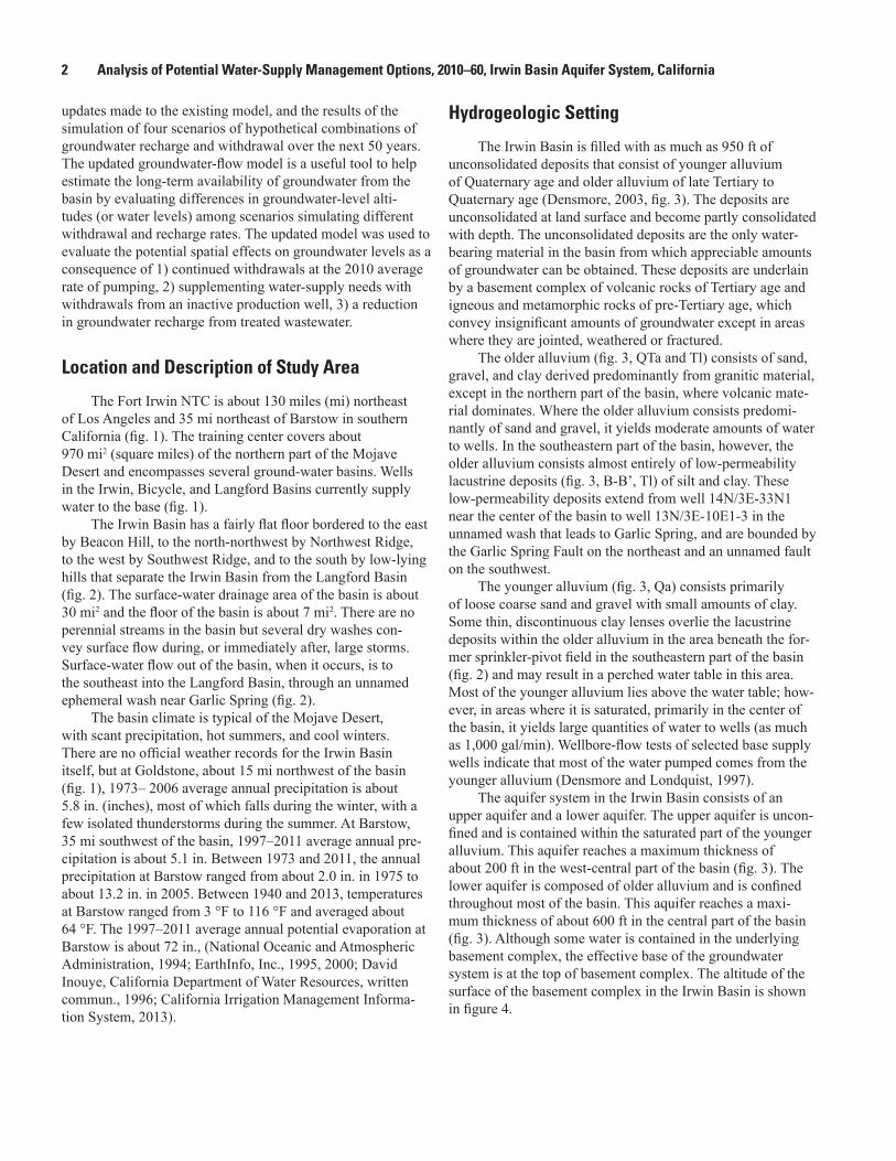
The Fort Irwin NTC is about 130 miles (mi) northeast of Los Angeles and 35 mi northeast of Barstow in southern California (fig. 1). The training center covers about 970 mi2 (square miles) of the northern part of the Mojave Desert and encompasses several ground-water basins. Wells in the Irwin, Bicycle, and Langford Basins currently supply water to the base (fig. 1).
The Irwin Basin has a fairly flat floor bordered to the east by Beacon Hill, to the north-northwest by Northwest Ridge, to the west by Southwest Ridge, and to the south by low-lying hills that separate the Irwin Basin from the Langford Basin (fig. 2). The surface-water drainage area of the basin is about 30 mi2 and the floor of the basin is about 7 mi2. There are no perennial streams in the basin but several dry washes con-vey surface flow during, or immediately after, large storms. Surface-water flow out of the basin, when it occurs, is to the southeast into the Langford Basin, through an unnamed ephemeral wash near Garlic Spring (fig. 2).
The basin climate is typical of the Mojave Desert, with scant precipitation, hot summers, and cool winters. There are no official weather records for the Irwin Basin itself, but at Goldstone, about 15 mi northwest of the basin (fig. 1), 1973– 2006 average annual precipitation is about 5.8 in. (inches), most of which falls during the winter, with a few isolated thunderstorms during the summer. At Barstow, 35 mi southwest of the basin, 1997–2011 average annual pre-cipitation is about 5.1 in. Between 1973 and 2011, the annual precipitation at Barstow ranged from about 2.0 in. in 1975 to about 13.2 in. in 2005. Between 1940 and 2013, temperatures at Barstow ranged from 3 °F to 116 °F and averaged about 64 °F. The 1997–2011 average annual potential evaporation at Barstow is about 72 in., (National Oceanic and Atmospheric Administration, 1994; EarthInfo, Inc., 1995, 2000; David Inouye, California Department of Water Resources, written commun., 1996; California Irrigation Management Informa-tion System, 2013).
Hydrogeologic Setting
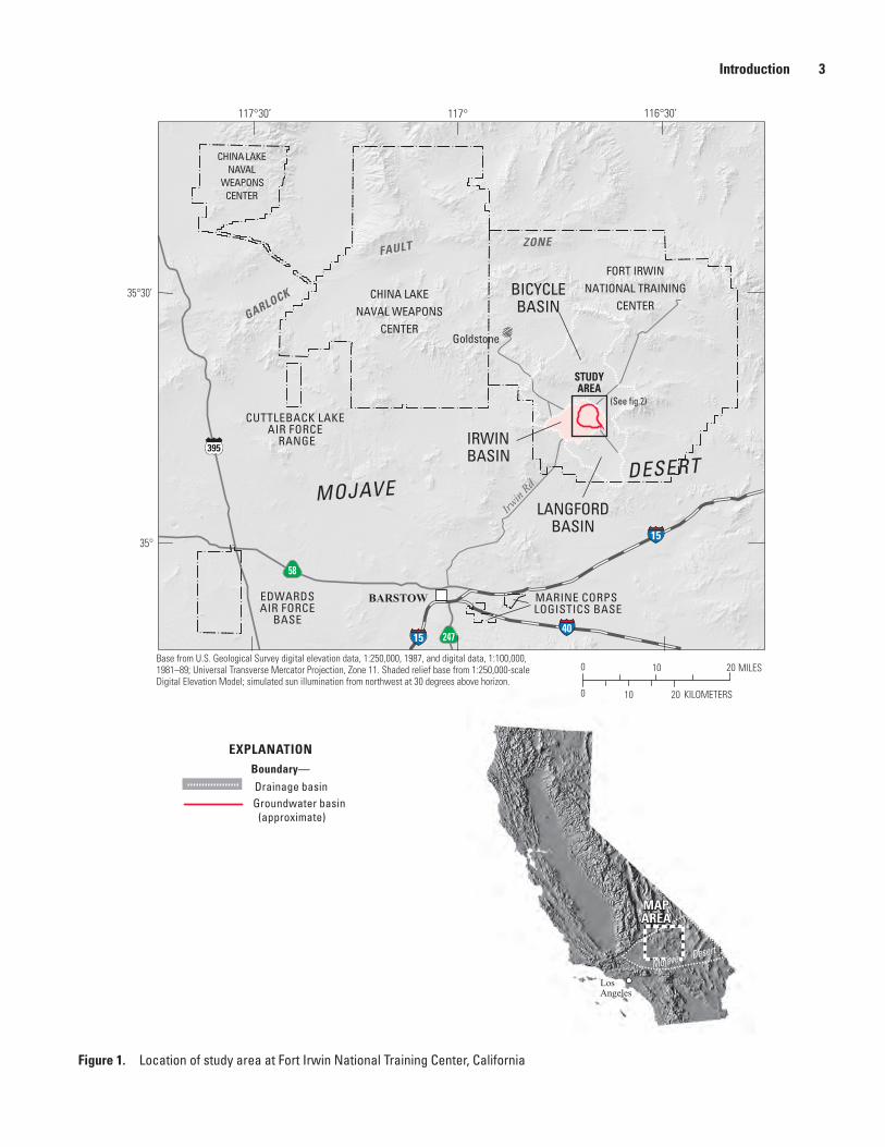
The Irwin Basin is filled with as much as 950 ft of unconsolidated deposits that consist of younger alluvium of Quaternary age and older alluvium of late Tertiary to Quaternary age (Densmore, 2003, fig. 3). The deposits are unconsolidated at land surface and become partly consolidated with depth. The unconsolidated deposits are the only water-bearing material in the basin from which appreciable amounts of groundwater can be obtained. These deposits are underlain by a basement complex of volcanic rocks of Tertiary age and igneous and metamorphic rocks of pre-Tertiary age, which convey insignificant amounts of groundwater except in areas where they are jointed, weathered or fractured.
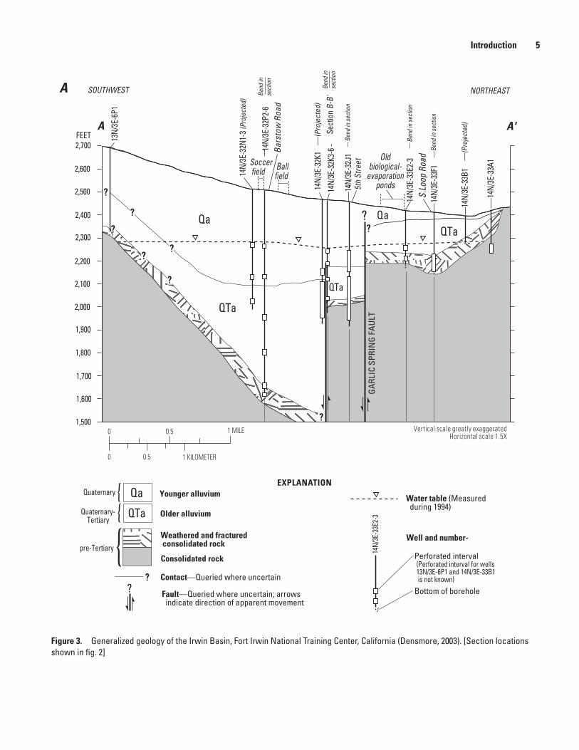
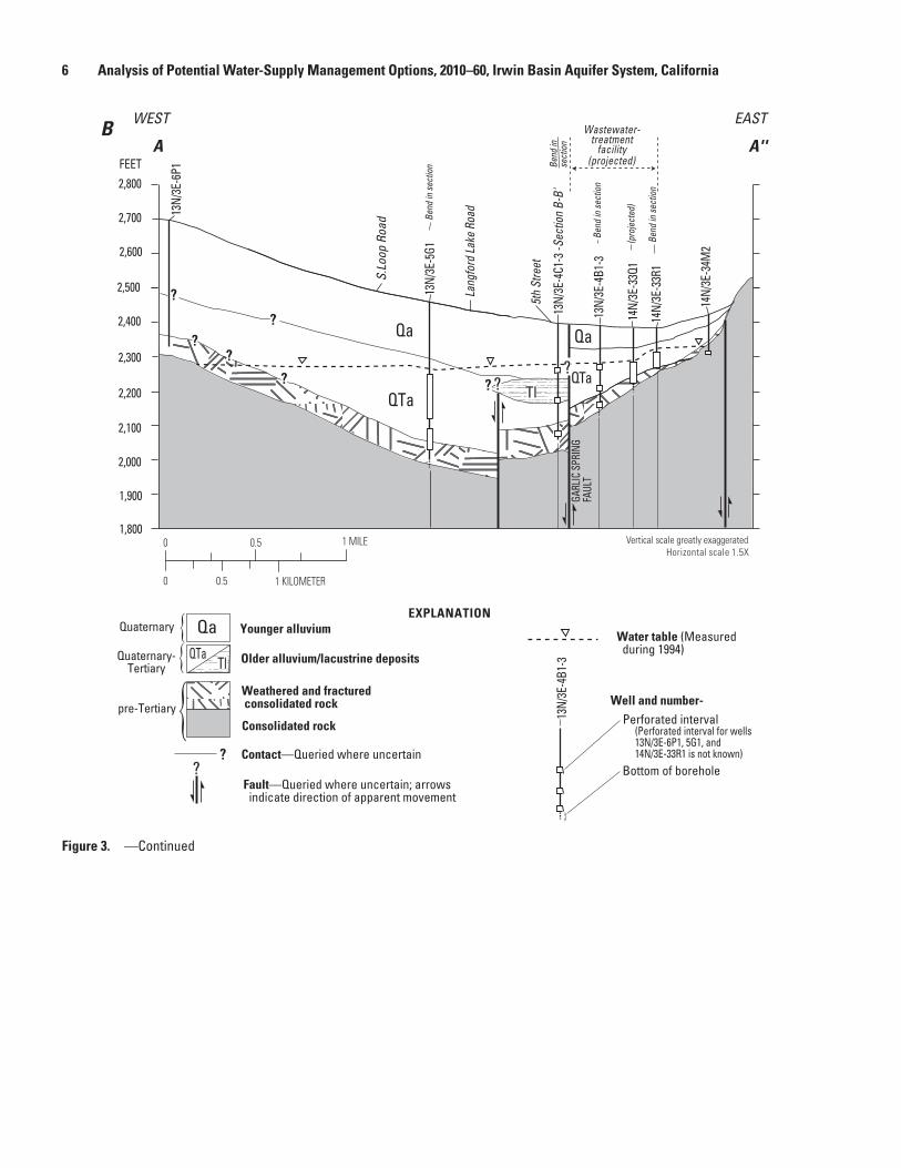
The older alluvium (fig. 3, QTa and Tl) consists of sand, gravel, and clay derived predominantly from granitic material, except in the northern part of the basin, where volcanic mate-rial dominates. Where the older alluvium consists predomi-nantly of sand and gravel, it yields moderate amounts of water to wells. In the southeastern part of the basin, however, the older alluvium consists almost entirely of low-permeability lacustrine deposits (fig. 3, B-B’, Tl) of silt and clay. These low-permeability deposits extend from well 14N/3E-33N1 near the center of the basin to well 13N/3E-10E1-3 in the unnamed wash that leads to Garlic Spring, and are bounded by the Garlic Spring Fault on the northeast and an unnamed fault on the southwest.
The younger alluvium (fig. 3, Qa) consists primarily of loose coarse sand and gravel with small amounts of clay. Some thin, discontinuous clay lenses overlie the lacustrine deposits within the older alluvium in the area beneath the for-mer sprinkler-pivot field in the southeastern part of the basin (fig. 2) and may result in a perched water table in this area. Most of the younger alluvium lies above the water table; how-ever, in areas where it is saturated, primarily in the center of the basin, it yields large quantities of water to wells (as much as 1,000 gal/min). Wellbore-flow tests of selected base supply wells indicate that most of the water pumped comes from the younger alluvium (Densmore and Londquist, 1997).
The aquifer system in the Irwin Basin consists of an upper aquifer and a lower aquifer. The upper aquifer is uncon-fined and is contained within the saturated part of the younger alluvium. This aquifer reaches a maximum thickness of about 200 ft in the west-central part of the basin (fig. 3). The lower aquifer is composed of older alluvium and is confined throughout most of the basin. This aquifer reaches a maxi-mum thickness of about 600 ft in the central part of the basin (fig. 3). Although some water is contained in the underlying basement complex, the effective base of the groundwater system is at the top of basement complex. The altitude of the surface of the basement complex in the Irwin Basin is shown in figure 4.
Introduction 3
Figure 1. Location of study area at Fort Irwin National Training Center, California
IRWINBASIN
BICYCLEBASIN
LANGFORDBASIN
EXPLANATION
Drainage basinGroundwater basin (approximate)
Boundary—
15
1540
58
247
395
LosAngeles
MAPAREA
Mojave DesertMojave Desert
Base from U.S. Geological Survey digital elevation data, 1:250,000, 1987, and digital data, 1:100,000, 1981–89; Universal Transverse Mercator Projection, Zone 11. Shaded relief base from 1:250,000-scaleDigital Elevation Model; simulated sun illumination from northwest at 30 degrees above horizon.
F.1
0 2010
0 2010
MILES
KILOMETERS
STUDYAREA
BARSTOW
117°30’ 117° 116°30’
35°
35°30’
MOJAVE DESERT
Irwin
Rd
FORT IRWINNATIONAL TRAINING
CENTERCHINA LAKE
NAVAL WEAPONSCENTER
CHINA LAKENAVAL
WEAPONSCENTER
GARLOCK
FAULT ZONE
CUTTLEBACK LAKEAIR FORCE
RANGE
EDWARDSAIR FORCE
BASE
MARINE CORPS LOGISTICS BASE
Goldstone
(See fig.2)

4 Analysis of Potential Water-Supply Management Options, 2010–60, Irwin Basin Aquifer System, California
LANGFORDBASIN
IRWIN
BASIN
BICYCLEBASIN
BeaconHill
BeaconHill
B
A'
A
A"
B'
GARLIC SPRING FAULT
Geology by J.C. Yount, E.R. Schermer, T.J. Felger, D.M. Miller, and K.A. Stephens, 1994Aquifer system boundary modified from Wilson F. So and Assoc., 1989
?
BICYCLE FAULT1
32K1
33N16
5
8
9
7
3
4
1
2
10
11
12
12
3
1010
5
4
7
8
9
2
Barsto
w Rd
Irwin R
d
N. Loop Rd
S. Loop Rd
Langford Lake Rd
5th St4K2-4
4Q2-6
33R1
4C1-3
10E1-3
4B1-3
32B1-3
Former sprinkler -pivot field
Duck ponds
Golf course and percolation pond
Soccer field
Baseball fieldSanitary-landfill facility
Old biological- evaporation ponds
Army ball fieldWastewater-treat- ment facility pond Base housing
New base housing
New athletic fields
Potential sources of groundwater degradation—
34M2
31
35°17’
35°13’
116°43’ 116°39'
6
36
T 14 N
T 13 N
R 2 E R 3 E
0
0 21 MILES
KILOMETERS21
EXPLANATION
SOUTHWEST
RIDGE
sac13-0507_Figure 02
6
1
Unconsolidated deposits—Correlation and description of map units
Quaternary-Tertiary
Consolidated rocks—
Well and number—
Installed by USGS
ProductionFault—Dashed where approximately located; queried where uncertain; dotted where concealed
Volcanic
Igneous and metamorphic
PlayaAlluvium
?
Line of geologic section—Sections shown on fig. 3
Boundary of aquifer system (approximate)
Test9B1
A"A
NORTHWEST RIDGE
GarlicSpring
{{
{Tertiary
pre-Tertiary
10D1
4D1-3
33N1
32N1-3
33E2-3
33A1
32P2-6
32K3-6?
33B1
32F132J1
32K133Q1
5G1
6P1
33F1
Drainage basin boundary
Figure 2. Generalized map of the Irwin Basin, Fort Irwin National Training Center, California.
Introduction 5
14N/
3E-3
2P2-
6
14N/
3E-3
2K1
14N/
3E-3
2K3-
6 -
14N/
3E-3
2J1
14N/
3E-3
3E2-
3
14N/
3E-3
3F1
14N/
3E-3
3A1
14N/
3E-3
2N1-
3 (Pr
ojec
ted)
13N/
3E-6
P1
SOUTHWEST NORTHEAST
?Qa Qa
QTa
QTa
QTa
2,600
2,700FEET
2,500
2,400
2,300
2,200
2,100
2,000
1,900
1,800
1,700
1,600
1,500
A A'
Soccer field Ball
field
Sect
ion
B-B'
—(P
roje
cted
)
?
?
5th
Stre
et
S.Lo
op R
oadB
arst
ow R
oad
Oldbiological-
evaporationponds
GA
RLIC
SPR
ING
FAU
LT
14N/
3E-3
3B1
—(P
roje
cted
)
Bend
in se
ctio
n
Bend
in se
ctio
n
Bend
in se
ctio
n
Bend
in
sect
ion
Bend
in
sect
ion
?
?
?
?
?
?
sac13-0507_Figure 03a
A
?
QTaWater table (Measured during 1994)
? Contact—Queried where uncertain
Fault—Queried where uncertain; arrows indicate direction of apparent movement
Well and number-
Perforated interval
Bottom of borehole
EXPLANATION
14N/
3E-3
3E2-
3
}
Qa
Consolidated rock
Younger alluvium
Older alluvium
Weathered and fractured consolidated rock
Quaternary
Quaternary-Tertiary
pre-Tertiary
(Perforated interval for wells13N/3E-6P1 and 14N/3E-33B1 is not known)
0 0.5
0 0.5 1 MILE
1 KILOMETER
Vertical scale greatly exaggeratedHorizontal scale 1.5X
Figure 3. Generalized geology of the Irwin Basin, Fort Irwin National Training Center, California (Densmore, 2003). [Section locations shown in fig. 2]
6 Analysis of Potential Water-Supply Management Options, 2010–60, Irwin Basin Aquifer System, California
WEST EAST
2,500
FEET
2,400
2,700
2,800
2,600
2,300
2,200
2,100
2,000
1,900
1,800
A A''
?
?
?
Vertical scale greatly exaggerated
13N/
3E-4
C1-3
-Sec
tion
B-B'
13N/
3E-5
G1
14N/
3E-3
3Q1
14N/
3E-3
3R1
13N/
3E-4
B1-3
14N/
3E-3
4M2
13N/
3E-6
P1
?
Lang
ford
Lake
Roa
d
5th
Stre
et
S.Lo
op R
oad
GARL
IC S
PRIN
G FA
ULT
13N/
3E-4
B1-3
Qa
QTa
Qa
QTa
Wastewater-treatment
facility(projected)
?
?
Water table (Measured during 1994)
? Contact—Queried where uncertain
Fault—Queried where uncertain; arrows indicate direction of apparent movement
Well and number-Perforated interval
Bottom of borehole
EXPLANATION
}
Qa
Consolidated rock
Younger alluvium
Older alluvium/lacustrine deposits
Weathered and fractured consolidated rock
Quaternary {{
{pre-Tertiary
Bend
in se
ctio
n
Bend
in
sect
ion
(pro
ject
ed)
Bend
in se
ctio
n
Bend
in se
ctio
n
QTaQuaternary-Tertiary
(Perforated interval for wells 13N/3E-6P1, 5G1, and 14N/3E-33R1 is not known)
Horizontal scale 1.5X
Tl
Tl?
??
?
0 0.5
0 0.5 1 MILE
1 KILOMETER
sac13-0507_Figure 03b
B
Figure 3. —Continued

Introduction 7
?
? ?
?
14N/
3E-3
3N1
14N/
3E-3
2B1-
3
14N/
3E-3
2K3-
6
14N/
3E-3
2F1
13N/
3E-4
D1-3
13N/
3E-4
C1-3
13N/
3E-4
Q2-6
13N
/3E-
4K2-
4
13N/
3E-1
0D1
13N/
3E-1
0E1-
3
SOUTHNORTH
2,600
2,700
2,900
2,800
FEET
2,500
2,400
2,300
2,200
2,100
2,000
1,900
1,800
Qa
Qa
Qa
QTaQTa
B B'
Formersprinkler- pivot field
Duckponds
13N/
3E-1
0E1-
3
Sect
ion
A-A"
Sect
ion
A-A'
Lysimeter and number
Vertical scale greatly exaggerated(P
roje
cted
)
5th
Stre
et
5th
Stre
et
}
13N/
3E-4
Q2-6
(Projected)
Bend
in
sect
ion
Bend
in
sect
ion
Bend
in
sect
ion
Bend
in
sect
ion
Bend
in
sect
ion
?
Water table (Measured during 1994)
? Contact—Queried where uncertainFault—Queried where uncertain; arrows indicate direction of apparent movement
Well and number-Perforated interval
Bottom of borehole
EXPLANATION
Qa
Consolidated rock
Younger alluvium
Older alluvium/ lacustrine depositsWeathered and fractured consol- idated rock
Quaternary {{
{pre-Tertiary
(Perforated interval for well13N/3E-10D1 is not known)
?
?
?
QTaQuaternary-Tertiary
Horizontal scale 1.5X
Tl
Tl
?
?
?
?
?
?
0 0.5
0 0.5 1 MILE
1 KILOMETER
sac13-0507_Figure 03c
C
Figure 3. —Continued
8 Analysis of Potential Water-Supply Management Options, 2010–60, Irwin Basin Aquifer System, California
25 30 40 50 6036
40
50
60
70
80
64MODEL COLUMN
MO
DEL
RO
W
1,900
2,000
2,2002,300
2,400
2,00
0
2,200
2,400
1,90
0
1,700
2,1002,100
2,100
2,300
1,900
1,800
2,300
2,200
2,300
35°15'
116°39'116°41'
35°17'
N
0
0 1 KILOMETER
1 MILE
Basement complex
Unconsolidated rocks
Model layer 2
Bedrock Contour—Shows altitude of bedrock. Contour interval 100 feet. Datum is sea level
2,100
EXPLANATION
Model grid
Model layer 1Boundaries–
Horizontal flow barrier (Model fault)
General head
Unnamed wash
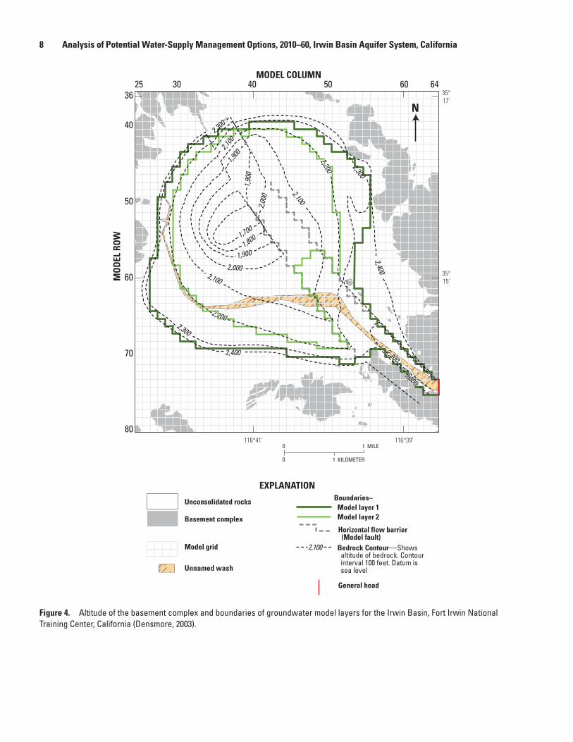
sac13-0507_Figure 04-basement complexFigure 4. Altitude of the basement complex and boundaries of groundwater model layers for the Irwin Basin, Fort Irwin National Training Center, California (Densmore, 2003).

Simulation of Groundwater Flow 9
Numerous faults have been mapped in the bedrock hills surrounding the Irwin Basin (Yount and others, 1994) (figs. 2, 3); they include the Garlic Spring Fault, the Bicycle Lake Fault, and many unnamed faults. Most of these faults are buried beneath the unconsolidated deposits and thus their presence within the basin is largely unknown. Yount and others (1994) mapped the Garlic Spring Fault into the uncon-solidated deposits, suggesting that the fault may cut through both the younger and the older alluvium in the southeastern part of the basin. Water-quality and water-level data, presented by Densmore and Londquist (1997), indicate that the Garlic Spring Fault and a parallel unnamed fault may be acting, in part, as a partial barrier to horizontal groundwater flow, primarily in the lower aquifer. The water-quality data indicate that vertical flow also is being impeded on the west side of the Garlic Spring Fault because of lithologic differences between the younger alluvium and the underlying lacustrine deposits of the older alluvium. Minor compaction and deformation of the water-bearing deposits immediately adjacent to the faults, fault gouge along the fault zone, and cementation of the fault zone by the deposition of minerals from groundwater are believed to create the barrier effect of the faults.
The areal extent of the aquifer system is defined by the intersection of the water table and the surrounding rocks of the basement complex. Under predevelopment condi-tions (pre-1941), the water table was about 2,300 feet above NAVD88. The boundary of the saturated aquifer system coincides with the 2,300-foot altitude contour of the basement complex shown in figure 4 (the approximate boundary of the aquifer system is shown in figure 2). All the alluvial deposits above this altitude were unsaturated under predevelopment conditions.
Simulation of Groundwater FlowAn existing groundwater-flow model of the aquifer
system in the Irwin Basin (Densmore, 2003) was updated and used to simulate flow under four alternative withdrawal and recharge conditions, here called scenarios. Densmore (2003) developed a two-layer groundwater-flow model for the period 1941–99 for the aquifer system in the Irwin Basin to assess the long-term availability and quality of groundwater, to evalu-ate groundwater conditions as a result of withdrawals, and to plan for future water needs at the base. Results of the model simulations of the scenarios were used to analyze the effects of the four alternative withdrawal and recharge conditions on the aquifer system.
Model Design
The existing groundwater-flow model was constructed using the USGS Modular Three-Dimensional Finite-Difference Groundwater- Flow Model (MODFLOW-88) developed by McDonald and Harbaugh (1988). For this study, the model input data was reformatted for a newer version of MODFLOW, MODFLOW-2005 (Harbaugh, 2005), and with-drawals were updated with 2000 to 2010 data. The updated model will be referred to in this report as the 2010 model.
The time intervals simulated in the original model were 1-year stress periods from January 1941 to December 1999. For the 2010 model, the time intervals simulated were years from January 1941 to December 2007, and months from January 2008 to December 2010.
The model grid developed for the original model was used for this study and is shown in figure 4. The origin of the model grid (the upper left corner of the grid; row 1, column 1) is at an easting of 2,373,237 ft and a northing of 669,380 ft in zone 5 of the California State Plane coordinate system. The grid consists of 80 rows and 64 columns with a cell size of 500 ft on a side (fig. 4).
The MODFLOW code consists of a main program and a series of independent subroutines called modules. The MODFLOW-2005 modules used in the 2010 model include Basic (BAS6); Block-Centered Flow (BCF6); General-Head Boundary (GHB); Drain (DRN); Discretization (DIS); Horizontal-Flow-Barrier (HFB6; Hsieh and Freckleton, 1993); Multi-Node Well (MNW2, Konikow and others, 2009); and Recharge (RCH) [BAS6, BCF6, GHB, DRN, and RCH, Harbaugh, 2005, MODFLOW-2005]. The original model (Densmore, 2003) used all of the above-mentioned modules except the MNW2, the WEL module (McDonald and Harbaugh, 1988) was used. For this study, the well input file was reformatted into the format for the MNW2 module. The 2010 model uses the Geometric Multigrid Solver (GMG, Wilson and Naff, 2004), whereas the original model used the Strongly Implicit Procedure Solver (SIP, McDonald and Harbaugh, 1988).
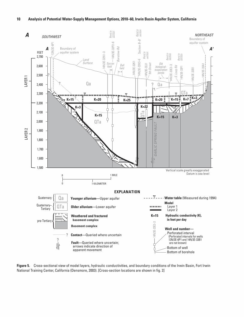
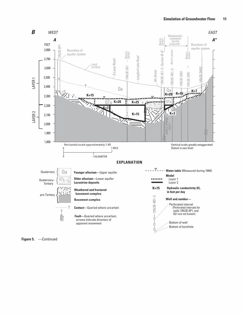
The model representation of the aquifer system, cali-brated aquifer properties, and model boundaries simulated in the original model were not changed for this study. The model representation of the aquifer system is shown in figure 5. Horizontal hydraulic conductivity of the aquifer system ranged from 3 to 25 ft/d (feet per day) for model layer 1 and 3 to 22 ft/d for layer 2. Model boundaries are shown in figure 4. The lateral boundaries of the model coincide with the lateral boundaries of the aquifer system. The top boundary of the
10 Analysis of Potential Water-Supply Management Options, 2010–60, Irwin Basin Aquifer System, California
sac13-0507_Figure 05a
Boundary ofaquifer system
Boundary ofaquifer system
14N/
3E-3
2P2–
6
14N/
3E-3
2K1
14N/
3E-3
2K3–
6
14N/
3E-3
2J1
14N/
3E-3
3E2–
3
14N/
3E-3
3F1
14N/
3E-3
3A1
14N/
3E-3
2N1–
3
13N/
3E-6
P1
SOUTHWEST NORTHEAST
?Qa Qa
QTa
QTa
2,600
2,700FEET
2,500
2,400
2,300
2,200
2,100
2,000
1,900
1,800
1,700
1,600
1,500
A A'
Soccer field
LandSurface
Ballfield
Sect
ion
B–B'
??
5th
Stre
et
S. L
oop
Rd
Bar
stow
Rd
Oldbiological-
evaporationponds
GA
RLIC
SPR
ING
FA
ULT
14N/
3E-3
3B1
Bend
in
sect
ion
Bend
in
sect
ion
Bend
in
sect
ion
Bend
in
sect
ion
Bend
in
sect
ion
?
?
Hydraulic conductivity (K), in feet per day
ModelLayer 1 Layer 2
K=15
K=3
K=20
K=15
K=25
K=22
K=15K=20
K=15 K=3
K=7 K=3
K=15
LAYE
R 1
LAYE
R 2
QTa
?
QTa
Water table (Measured during 1994)
? Contact—Queried where uncertain
Fault—Queried where uncertain; arrows indicate direction of apparent movement
Well and number—Perforated interval
Bottom of boreholeBottom of well
EXPLANATION
14N/
3E-3
3E2–
3
}
Qa
Basement complex
Younger alluvium—Upper aquifer
Older alluvium—Lower aquifer
Weathered and fractured basement complex
Quaternary
Quaternary–Tertiary
{{
{pre-Tertiary
(Perforated intervals for wells13N/3E-6P1 and 14N/3E-33B1 are not known)
Vertical scale greatly exaggerated
0
0 1 MILE Datum is sea level
1 KILOMETER
?
?
?
?
?
A
Figure 5. Cross-sectional view of model layers, hydraulic conductivities, and boundary conditions of the Irwin Basin, Fort Irwin National Training Center, California (Densmore, 2003). [Cross-section locations are shown in fig. 2]
Simulation of Groundwater Flow 11
?
?
?
13N/
3E-4
C1–3
-Sec
tion
B–B'
13N/
3E-5
G1
14N/
3E-3
3Q1
14N/
3E-3
3R1
13N/
3E-4
B1–3
14N/
3E-3
4M2
13N/
3E-6
P1
?
Lang
ford
Lake
Roa
d
5th
Stre
et
S.Lo
op R
oad
GARL
IC S
PRIN
G
FAU
LT
Qa Qa
QTa QTa
Wastewater-treatment
facility
Landsurface
(projected)
?
Bend
in se
ctio
n
Bend
in
sect
ion
Bend
in
sect
ion
Bend
in
sect
ion
?
???
? K=15
K=20
K=3
K=3
K=25
K=7K=15
K=15
K=20
Hydraulic conductivity (K),in feet per day
ModelLayer 1 Layer 2
K=15
Water table (Measured during 1994)
13N/
3E-4
B1–3 Well and number—
Perforated interval
Bottom of boreholeBottom of well
}
(Perforated intervals for wells 13N/3E-6P1, and 5G1 are not known)
0
0 1 MILE Datum is sea level
1 KILOMETER
Vertical scale greatly exaggerated
?? Contact—Queried where uncertain
Fault—Queried where uncertain; arrows indicate direction of apparent movement
EXPLANATION
Qa
Basement complex
Younger alluvium—Upper aquifer
Older alluvium—Lower aquiferLacustrine deposits
Weathered and fractured basement complex
Quaternary {{
{ pre-Tertiary
QTaQuaternary–Tertiary
Horizontal scale approximately 1.4X
Tl
LAYE
R 1
LAYE
R 2
2,500
2,400
2,700
2,600
2,300
2,200
2,100
2,000
1,900
1,800
2,800FEET
WEST EAST
A A"Boundary ofaquifer systemBoundary of
aquifer system
B
Tl
sac13-0507_Figure 05b
Figure 5. —Continued

12 Analysis of Potential Water-Supply Management Options, 2010–60, Irwin Basin Aquifer System, California
?
?? ?
?
14N/
3E-3
3N1
14N/
3E-3
2B1–
3
14N/
3E-3
2K3–
6
14N/
3E-3
2F1
13N/
3E-4
D1–3
13N/
3E-4
C1–3
13N/
3E-4
Q2–6
13N
/3E-
4K2–
4
13N/
3E-1
0D1
13N/
3E-1
0E1–
3
Qa
QaQa
Qa
QTa
QTa
Formersprinkler- pivot field
Duckponds
Sect
ion
A–A"
Sect
ion
A–A
'
(Pro
ject
ed)
5th
Stre
et
5th
Stre
et
(Projected)
Bend
in
sect
ionBe
nd in
se
ctio
n
Bend
in
sect
ion
Bend
in
sect
ion
Bend
in
sect
ion
LAYE
R 1
LAYE
R 2 ?
?
?
SOUTHNORTH
2,600
2,700
2,900
2,800
FEET
2,500
2,400
2,300
2,200
2,100
2,000
1,900
1,800
B B'
?
K=20K=25K=20
K=22K=15
K=25
?
K=3
?
LIX3
Hydraulic conductivity (K), in feet per day
ModelLayer 1 Layer 2
K=15
Water table (Measured during 1994)
Boundary ofaquifer system
Boundary ogaquifer system
? Contact—Queried where uncertain
EXPLANATION
LIX3
13
N/3E
-10E
1–3
Lysimeter and number
}
13N/
3E-4
Q2–6
Well and number—Perforated interval
Bottom of boreholeBottom of well
Destroyed well and number
Qa
Basement complex
Younger alluvium—Upper aquifer
Older alluvium—Lower aquiferLacustrine deposits
Weathered and fractured basement complex
Quaternary {{
{pre-Tertiary
(Perforated interval for well LIX-3 is not known)QTaQuaternary-
Tertiary Tl
0 1 KILOMETER
Vertical scale greatly exaggeratedDatum is sea level
0 1 MILE
??
Landsurface
C
Tl
sac13-0507_Figure 05c
Figure 5. —Continued
model, the water table, is simulated as a free-surface bound-ary (unconfined) to allow vertical movement in response to changes between inflow and outflow. No-flow boundaries are used around and below the modeled area to represent contact with the basement complex. The HFB6 package was used to simulate the 2 faults that impede the horizontal flow of groundwater. The GHB package was used to simu-late underflow from layer 1 through the unnamed wash near Garlic Spring. The reader is referred to Densmore (2003) for a detailed description of the aquifer system framework, aquifer properties and model boundaries.
Model Calibration
The 2010 model was not re-calibrated, but the results of the simulations made with the original model and the 2010 model were compared to ensure that the original level of cali-bration was maintained. Simulated 1994 hydraulic heads (or potentiometric surface) from the original model (Densmore, 2003, fig. 19) were compared with those heads simulated in the 2010 model (fig. 6). The comparisons were only visual, however, because the original 1994 hydraulic heads generated by Densmore (2003) were not archived in GIS format. Model
budgets calculated for each stress period by MODFLOW in the original and 2010 model were also compared. The original list file, lst.trand114, containing the model budgets, can be requested from the USGS California Water Science Center, San Diego, Calif.
The update of the original model was done in steps to allow for evaluation and analysis of simulation results and to maintain the original level of calibration. First, the original model input data was reformatted from MODFLOW-88 to MODFLOW-2005 format, and then the well input file was reformatted to the newer MNW2 format. The simulated 1994 hydraulic heads, generated from the original model data that had been reformatted to run with MODFLOW-2005, are shown in red in figure 6 and compare well with the original 1994 hydraulic heads generated by Densmore (2003). The MODFLOW-2005 model input data was then run with the original well data reformatted for the MNW2 module. The simulated 1994 hydraulic heads, generated from the 2010 model with the MNW2 well data, are shown in purple in figure 6 and are slightly different in the area of the production wells 14N/3E-32F1, 14N/3E-32H1 and 14N/3E-32K1 (fig. 6) from the hydraulic heads simulated by using the original well data. Using the MNW2 module, the simulated 1994 hydraulic heads for layer 1 at production wells 14N/3E-32H1 and

Simulation of Groundwater Flow 13
Figure 6. Simulated 1994 hydraulic heads, layer 1, Irwin Basin, Fort Irwin National Training Center, California.
LANGFORDBASIN
IRWIN
BASIN
BICYCLEBASIN
BeaconHill
BeaconHill
GARLIC SPRING FAULT
Geology by J. C. Yount, E.R. Schermer, T.J. Felger, D.M. Miller, and K.A. Stephens, 1994Aquifer system boundary modified from Wilson F. So and Assoc., 1989
?
BICYCLE FAULT
2,280
2,285
2,290
2,29
5
2,30
0
2,275
2,305
2,310
2,315
2,270
2,320
2,325
2,2552,2
65
2,245
2,280
2,300
2,290
2,305
2,310
2,270
2,280
1
Barsto
w Rd
Irwin R
d
N. Loop Rd
S. Loop Rd
Langford Lake Rd
Infiltration pond
Athletic field
Road
31
35°17’
35°13’
116°43’ 116°39'
6
36 T 14 N
T 13 N
R 2 E R 3 E
0
0 21 MILES
KILOMETERS21
EXPLANATION
SOUTHWEST
RIDGE
sac13-0507_Figure 06
Unconsolidated deposits—Correlation and description of map units
Quaternary-Tertiary
Consolidated rocks—
Well and number—Fault—Dashed where approximately located; queried where uncertain; dotted where concealed
Volcanic
Igneous and metamorphic
PlayaAlluvium
?
NORTHWEST RIDGE
GarlicSpring
{{
{Tertiary
pre-Tertiary
?
32H132F1
32K1
Extent of model layer 1
Simulated 1994 hydraulic-head contour, using MODFLOW 2005 with the well module. Contour interval is 5 feet. Datum is NAVD88 Simulated 1994 hydraulic-head contour, using MODFLOW 2005 with the MNW2 module. Contour interval is 5 feet. Datum is NAVD88 32K1
Boundary of aquifer system (approximate)Drainage basin boundary

14 Analysis of Potential Water-Supply Management Options, 2010–60, Irwin Basin Aquifer System, California
14N/3E-32K1 are 2.61 and 3.51 ft higher, respectively, than the 1994 simulated hydraulic heads using the WEL module. In contrast, the 1994 hydraulic heads simulated by using the MNW2 module for layer 2 at production wells 14N/3E-32F1, 14N/3E-32H1 and 14N/3E-32K1 are 1.28, 0.88 and 1.09 ft lower, respectively, than the 1994 simulated hydraulic heads using the WEL module. With the exception of the hydrau-lic heads within the closed 2,270-foot contour line (fig. 6), hydraulic heads from both models agree within 0.1 foot. This difference in hydraulic head may be attributed to how the withdrawals were distributed in the original model. The withdrawals from production wells were initially distributed as two-thirds from layer 1 and one-third from layer 2; this initial distribution was then varied between the two layers during calibration in the original model (Densmore, 2003). For the 2010 model, the percentage of groundwater withdrawals from each model layer was calculated by the MNW2 module.
The volumetric model budgets, calculated by MODFLOW, for the original MODFLOW-88 model and the 2010 model for 1994 conditions, which is stress period 54, are shown in table 1. Slight differences in the values for storage and head dependent boundary are probably a result of the difference in the distribution of withdrawals of the production wells calculated by the MNW2 module. Overall, the budget items compare well.
Hydrographs for 11 selected observation wells are shown in figure 7. Wells were selected on the basis of loca-tion and number of water-level measurements available, and only wells screened in a single layer were considered. The measured water levels and simulated hydraulic heads from the 2010 model are within 11 ft. Simulated hydraulic heads also matched the upward 1992–2010 trend in measured water levels. The upward trend is probably a result of recharge from the ponds near the wastewater-treatment facility and irrigation at the training center’s base housing.
Groundwater Withdrawals
The original model simulated hydrologic conditions from January 1941 to December 1999 with yearly stress periods. In the original model, groundwater withdrawals were aver-aged for the year. The 2010 model included 2000 to 2010 withdrawal data. Monthly groundwater withdrawal records were available for January 2000 through December 2010. For the 2010 model, groundwater withdrawals were simulated for 1-year periods from January 1941 to December 2007 and for 1-month periods from January 2008 to December 2010. Annual groundwater withdrawals from Bicycle, Irwin, and Langford Basins are shown in figure 8.
Groundwater Recharge
There are two sources of recharge to the aquifer system in the Irwin Basin: natural recharge from precipitation and artifi-cial recharge from wastewater-effluent infiltration at the ponds and irrigation-return flow (Densmore, 2003). Natural recharge in the basin is low because of low precipitation and high evap-oration rates. The calibrated natural recharge simulated in the original model was about 50 acre-ft/yr. The natural recharge was simulated along the intermittent unnamed wash shown in figure 4. The natural recharge of 50 acre-ft/yr was used in the 2010 model and simulated in the same model cells as those in the original model that represent the intermittent unnamed wash. Groundwater is imported to the Irwin Basin from Bicycle and Langford Basins. Some water is used for irriga-tion at the base housing; the water that is not consumed is treated at the wastewater-treatment facility and discharged to the infiltration ponds, referred to as the wastewater treatment facility pond, golf course pond and duck ponds. Estimated groundwater recharge has exceeded groundwater withdrawals
Table 1. Simulated volumetric budget, for 1994 conditions (stress period 54), from the A) original, MODFLOW-88 model and B) 2010 model, Irwin Basin, Fort Irwin National Training Center, California.
[ Values in cubic feet per day. Abbreviation: —, none]
Budget componentOriginal model (MODFLOW-88)
2010 model (MODFLOW-2005)
Percent difference between original and 2010 model
Inflow:Storage 6,054.70 5,951.50 0.07Recharge 152,271.55 152,271.61 –0.00Total in 158,330.00 158,223.11 —
Outflows:Storage 7,627.10 7,517.36 0.07Groundwater withdrawals 140,691.00 140,691.00 0.00Head dependent boundary 9,998.90 10,015.42 –0.01Total out 158,320.00 158,223.78 —
Inflow–outflow 9.20 –0.67 —Percent discrepancy 0.01 0.00 —

Simulation of Groundwater Flow 15
Figure 7. Hydrographs of measured water levels and simulated hydraulic heads in 11 observation wells, Irwin Basin, Fort Irwin National Training Center, California. [Well location shown in fig. 11]
201020001990198019701960195019412,240
2,260
2,280
2,300
2,320
2,340
201020001990198019701960195019412,240
2,260
2,280
2,300
2,320
2,340
201020001990198019701960195019412,240
2,260
2,280
2,300
2,320
2,340
201020001990198019701960195019412,240
2,260
2,280
2,300
2,320
2,340
201020001990198019701960195019412,240
2,260
2,280
2,300
2,320
2,340
201020001990198019701960195019412,240
2,260
2,280
2,300
2,320
2,340
201020001990198019701960195019412,240
2,260
2,280
2,300
2,320
2,340
201020001990198019701960195019412,240
2,260
2,280
2,300
2,320
2,340
201020001990198019701960195019412,240
2,260
2,280
2,300
2,320
2,340
201020001990198019701960195019412,240
2,260
2,280
2,300
2,320
2,340
201020001990198019701960195019412,240
2,260
2,280
2,300
2,320
2,340
EXPLANATION
Simulated value, layer 1
Measured value, well screened in layer 1
Simulated value, layer 2
Measured value, well screened in layer 2
Wat
er-le
vel a
ltitu
de, i
n fe
et a
bove
NAV
D 88
Figure 7a. Hydrographs of simulated and measured water levels in 11 observation wells, Fort Irwin National Training Center, California. (Well location shown in figure 11)
4D24D2 4D34D3
32B232B2 32B332B3
32K432K4 32K632K6
32P432P4 32P632P6
32F232F2 32F332F3
33E333E3
Year
Year

16 Analysis of Potential Water-Supply Management Options, 2010–60, Irwin Basin Aquifer System, California
Figure 8. Annual groundwater recharge and withdrawals from Bicycle, Irwin, and Langford Basins, Fort Irwin National Training Center, California, 1941–2010.
0
500
1,000
1,500
2,000
2,500
3,000
3,500
1941
19
43
1945
19
47
1949
19
51
1953
19
55
1957
19
59
1961
19
63
1965
19
67
1969
19
71
1973
19
75
1977
19
79
1981
19
83
1985
19
87
1989
19
91
1993
19
95
1997
19
99
2001
20
03
2005
20
07
2009
Rech
arge
and
with
draw
al, i
n ac
re-fe
et
Year
Figure 8. Annual groundwater recharge and withdrawals from Bicycle, Irwin, andLangford Basins, Fort Irwin National Training Center, California, 1941-2010.
Irwin Basin withdrawal Bicycle Basin withdrawal Langford Basin withdrawal Total estimated recharge in Irwin Basin
EXPLANATION
in the Irwin Basin since 1967, except for the years 1984 and 1986–91. From 1967, about 33,980 acre-ft was withdrawn from the groundwater-flow system within the Irwin Basin and an estimated 50,600 acre-ft recharged the basin, resulting in a net gain of 16,620 acre-ft of water to the groundwater-flow system (fig. 8 and table 2). Reduced pumping in the Irwin Basin, recharge from irrigation at the base housing, and artifi-cial recharge from treated wastewater at the infiltration ponds has caused water levels to stabilize or rise throughout most of the Irwin Basin (fig. 7).
The recharge rate used in the original model at the recreational fields (soccer, baseball, and Army ball fields) and grass areas at the base housing (fig. 2) was used in the 2010 model for January 2000 to December 2007. Additional base housing (fig. 2) was constructed in phases during May 2005, May 2008, and November 2008. Recharge was simulated in the 2010 model for these areas beginning in 2005. The original model simulated an average yearly recharge rate, in cubic feet per day, from January 1941 to December 1999. The recharge rate simulated in the original model was used in the 2010 model for the monthly stress periods from January 2008 to December 2010. At the recreational fields and grass areas at the base housing, the recharge rate was decreased by half for the winter months, January, February, November and December.
Estimates of daily evaporation and evapotranspiration from studies by the California Department of Water Resources (DWR) and the California Irrigation Management Information System (CIMIS) of DWR’s Office of Water Use Efficiency, respectively, were used in the calculation of water available for monthly recharge at the wastewater infiltration ponds (pond locations shown in fig. 2), where outflow from the wastewater-treatment facility is discharged in the Irwin Basin. Using an annual evaporation rate of 5.7 ft, the 2010 evapora-tion from the surface of wastewater infiltration ponds (area of ponds is 47 acres) was estimated to be about 270 acre-ft (table 3). Using an annual evapotranspiration rate of 6 ft, the 2010 evapotranspiration from the area (about 40 acres) around the wastewater infiltration ponds was estimated to be 240 acre-ft. There are no data available on the depth to groundwater within 500 ft of the ponds from wells screened within 20 ft of land surface. The well nearest to any of the infiltration ponds (pond locations shown in fig. 2) is obser-vation well 13N/3E-10D1, screened 15 to 65 ft below land surface and located about 500 ft southeast of the southernmost duck pond. The water level in this well was 15 ft below land surface on October 21, 2010. A shallow depth to groundwater was assumed for the area around the ponds because of the vegetation growing there, and the water from the ponds would flow laterally, in addition to vertically, into the surrounding aquifer. A shallow depth to groundwater, less than 10 ft, was

Simulation of Groundwater Flow 17
Year Withdrawal Recharge1941 33 491942 130 711943 350 1991944 480 2731945 182 1021946 57 501947 55 491948 55 491949 55 491950 55 501951 293 1661952 336 1931953 671 3851954 668 3821955 598 4881956 602 711957 704 791958 686 701959 655 701960 746 991961 881 1951962 1,119 3441963 1,147 3701964 1,202 4081965 1,305 6071966 1,509 7901967 827 9281968 764 8641969 727 9471970 549 7421971 364 4211972 399 7851973 321 4471974 200 3521975 236 421
Year Withdrawal Recharge1976 236 5691977 64 2241978 283 7021979 502 8831980 721 1,3881981 660 7021982 630 6661983 720 9011984 1,675 1,5581985 1,133 1,5481986 1,315 1,0061987 1,927 1,2571988 1,700 1,1731989 1,696 1,0731990 1,868 1,3901991 1,331 1,0221992 1,110 1,1461993 997 1,1961994 1,180 1,2761995 1,270 1,6451996 1,138 1,5681997 580 1,3431998 484 1,4601999 781 1,4602000 612 1,4622001 331 1,6402002 333 1,7162003 168 1,7812004 301 1,6712005 370 1,7012006 592 1,7332007 755 1,6902008 826 1,3852009 765 1,3762010 536 1,391
Table 2. Simulated annual 1941–2010 groundwater recharge and withdrawals, Irwin Basin, Fort Irwin National Training Center, California.
[Values in acre-feet per year.]

18 Analysis of Potential Water-Supply Management Options, 2010–60, Irwin Basin Aquifer System, CaliforniaTa
ble
3.
Sum
mar
y of
200
1–10
gro
undw
ater
with
draw
als,
and
est
imat
es o
f eva
potra
nspi
ratio
n, e
vapo
ratio
n, a
nd re
char
ge u
sed
in th
e 20
10 m
odel
and
mod
el s
cena
rios,
Irw
in
Basi
n, F
ort I
rwin
Nat
iona
l Tra
inin
g Ce
nter
, Cal
iforn
ia.
[Num
bers
in p
aren
thes
es a
re m
odel
cel
l num
bers
(row
, col
umn)
. Sce
nario
1 a
nd 3
do
not h
ave
a de
crea
se in
rech
arge
in p
hase
s. Sc
enar
io 2
, pha
se 1
use
s Sce
nario
1 re
char
ge v
alue
s. Sc
enar
io 2
, pha
se 4
has
no
rech
arge
in th
e ar
ea o
f the
pon
ds n
ear t
he w
aste
wat
er tr
eatm
ent f
acili
ty. V
alue
s in
acre
-fee
t unl
ess n
oted
oth
erw
ise.
Abb
revi
atio
n: C
A, C
alifo
rnia
; NE,
Nor
thea
st; -
>, in
dica
tes r
ange
of c
ells
in c
olum
n; #
, nu
mbe
r] Mon
th
Gro
undw
ater
w
ithdr
awal
sTr
eate
d w
aste
wat
erEv
apor
atio
nEv
apot
rans
pira
tion
Tota
l es
timat
ed
evap
orat
ion
and
evap
otra
ns-
pira
tion
in
Irw
in B
asin
Sim
ulat
ed 2
010
was
tew
ater
rech
arge
Aver
age
2001
–10
from
all
basi
ns1
2010
from
al
l bas
ins1
2010
to
was
tew
ater
tr
eatm
ent
faci
lity2
Aver
age
from
a
wat
er
surf
ace,
fe
et p
er
mon
th3
Estim
ated
fr
om th
e su
rfac
e of
po
nds
in
Irw
in
Bas
in4
San
Ber
nard
ino,
B
arst
ow, C
A
NE
- #13
4,
feet
per
mon
th5
Estim
ated
ev
apot
rans
-pi
ratio
n
from
are
as
arou
nd p
onds
in
Irw
in B
asin
6
Duc
k po
nds
(64,
55; 6
5,55
; 66
,55;
67,
55;
68,5
5)
Gol
f cou
rse
pond
(5
9,53
; 60,
53;
61,5
3; 6
2,53
; 62
,54;
63,
53;
63,5
4)
Was
tew
ater
-tr
eatm
ent
faci
lity
pond
(5
6,52
->53
; 57
,51-
>53;
58
,51-
>52;
59
,51-
>52;
60
,51-
>52)
Tota
l si
mul
ated
re
char
ge
from
pon
ds
in Ir
win
B
asin
Janu
ary
145
150
109
0.11
50.
187
1230
1815
63Fe
brua
ry13
614
610
60.
178
0.24
1018
2817
1459
Mar
ch18
119
210
70.
3315
0.45
1833
2917
1359
Apr
il20
019
593
0.50
240.
5924
4719
119
40M
ay25
523
795
0.73
340.
7530
6419
117
38Ju
ne27
926
287
0.87
410.
8534
7518
116
35Ju
ly30
028
410
40.
9243
0.83
3376
149
628
Aug
ust
282
294
115
0.81
380.
7429
6715
96
29Se
ptem
ber
276
273
940.
5827
0.57
2350
1811
736
Oct
ober
243
217
980.
3717
0.41
1634
1710
634
Nov
embe
r18
414
691
0.19
90.
239
1814
87
30D
ecem
ber
153
130
920.
105
0.17
711
2012
940
Tota
l of c
olum
n72,
635
2,52
61,
191
5.67
267
5.99
240
506
241
145
106
492

Simulation of Groundwater Flow 19Ta
ble
3.
Sum
mar
y of
200
1–10
gro
undw
ater
with
draw
als,
and
est
imat
es o
f eva
potra
nspi
ratio
n, e
vapo
ratio
n, a
nd re
char
ge u
sed
in th
e 20
10 m
odel
and
mod
el s
cena
rios,
Irw
in
Basi
n, F
ort I
rwin
Nat
iona
l Tra
inin
g Ce
nter
, Cal
iforn
ia.—
Cont
inue
d
[Num
bers
in p
aren
thes
es a
re m
odel
cel
l num
bers
(row
, col
umn)
. Sce
nario
1 a
nd 3
do
not h
ave
a de
crea
se in
rech
arge
in p
hase
s. Sc
enar
io 2
, pha
se 1
use
s Sce
nario
1 re
char
ge v
alue
s. Sc
enar
io 2
, pha
se 4
has
no
rech
arge
in th
e ar
ea o
f the
pon
ds n
ear t
he w
aste
wat
er tr
eatm
ent f
acili
ty. V
alue
s in
acre
-fee
t unl
ess n
oted
oth
erw
ise.
Abb
revi
atio
n: C
A, C
alifo
rnia
; NE,
Nor
thea
st; -
>, in
dica
tes r
ange
of c
ells
in c
olum
n; #
, num
-be
r]
Mon
th
Scen
ario
1,
Janu
ary
2011
thro
ugh
Dec
embe
r 206
0Sc
enar
io 2
, ph
ase
2, J
anua
ry 2
012
thro
ugh
Dec
embe
r 201
3Sc
enar
io 2
, ph
ase
3, J
anua
ry 2
014
thro
ugh
Dec
embe
r 201
5
Estim
ated
qu
antit
y of
trea
ted
was
tew
ater
di
scha
rge
to
pon
ds in
Ir
win
Bas
in8
Sim
ulat
ed w
aste
wat
er re
char
ge
Estim
ated
qu
antit
y of
trea
ted
was
tew
ater
di
scha
rge
to
pon
ds in
Ir
win
Bas
in8
Sim
ulat
ed w
aste
wat
er re
char
ge
Estim
ated
qu
antit
y of
trea
ted
was
tew
ater
di
scha
rge
to p
onds
in
Irw
in B
asin
8
Sim
ulat
ed w
aste
wat
er re
char
ge
Duc
k
pond
s (6
4,55
; 65
,55;
66
,55;
67
,55;
68
,55)
Gol
f co
urse
po
nd
(59,
53;
60,5
3; 6
1,53
; 62
,53;
62,
54;
63,5
3; 6
3,54
)
Was
tew
ater
-tr
eatm
ent
faci
lity
po
nd
(56,
52->
53;
57,5
1->5
3;
58,5
1->5
2;
59,5
1->5
2;
60,5
1->5
2)
Tota
l si
mul
ated
re
char
ge
from
po
nds
in
Irw
in
Bas
in
Duc
k
pond
s (6
4,55
; 65
,55;
66
,55;
67
,55;
68
,55)
Gol
f co
urse
po
nd
(59,
53; 6
0,53
; 61
,53;
62,
53;
62,5
4; 6
3,53
; 63
,54)
Was
tew
ater
tr
eatm
ent
faci
lity
po
nd
(56,
52->
53;
57,5
1->5
3;
58,5
1->5
2;
59,5
1->5
2;
60,5
1->5
2)
Tota
l si
mul
ated
re
char
ge
from
po
nds
in
Irw
in
Bas
in
Janu
ary
103
3018
1563
101
3018
1563
9830
1815
63Fe
brua
ry10
028
1714
5997
2817
1459
9328
1714
59M
arch
9329
1713
5986
2917
1359
7929
1713
59A
pril
7119
119
4061
1911
940
500
00
0M
ay66
96
419
510
00
036
00
00
June
550
00
039
00
00
220
00
0Ju
ly70
00
00
530
00
037
00
00
Aug
ust
830
00
067
00
00
500
00
0Se
ptem
ber
650
00
051
00
00
360
00
0O
ctob
er77
1710
634
6617
106
3455
95
317
Nov
embe
r77
148
730
7014
87
3064
148
730
Dec
embe
r86
2012
940
8320
129
4080
2012
940
Tota
l of c
olum
n794
616
610
078
344
823
157
9475
325
701
129
7762
269
1 Gro
undw
ater
with
draw
als f
rom
Bic
ycle
, Irw
in, a
nd L
angf
ord
Bas
ins.
2 Val
ues f
rom
For
t Irw
in N
atio
nal T
rain
ing
Cen
ter p
erso
nnel
.3 P
oten
tial e
vapo
ratio
n va
lues
from
pan
s dow
nloa
d fr
om h
ttp://
ww
w.w
ater
.ca.
gov.
4 Eva
pora
tion
estim
ated
from
mon
thly
pan
eva
pora
tion
mul
tiplie
d by
an
estim
ated
are
a of
47
acre
s for
all
pond
s.5 P
oten
tial e
vapo
trans
pira
tion
valu
es d
ownl
oad
from
Janu
ary
1, 1
997
thro
ugh
May
31,
200
1; h
ttp://
ww
wci
mis
.wat
er.c
a.go
v/ci
mis
/fron
tMon
thly
Repo
rt.d
o.6 E
vapo
trans
pira
tion
estim
ated
from
mon
thly
eva
potra
nspi
ratio
n va
lues
and
mul
tiplie
d by
an
estim
ated
are
a of
40
acre
s (ar
ea a
roun
d al
l pon
ds w
ith so
me
vege
tatio
n).
7 Val
ues m
ay n
ot a
dd to
tota
ls d
ue to
roun
ding
. 8 E
stim
ated
val
ues f
rom
For
t Irw
in N
atio
nal T
rain
ing
Cen
ter p
erso
nnel
.
20 Analysis of Potential Water-Supply Management Options, 2010–60, Irwin Basin Aquifer System, California
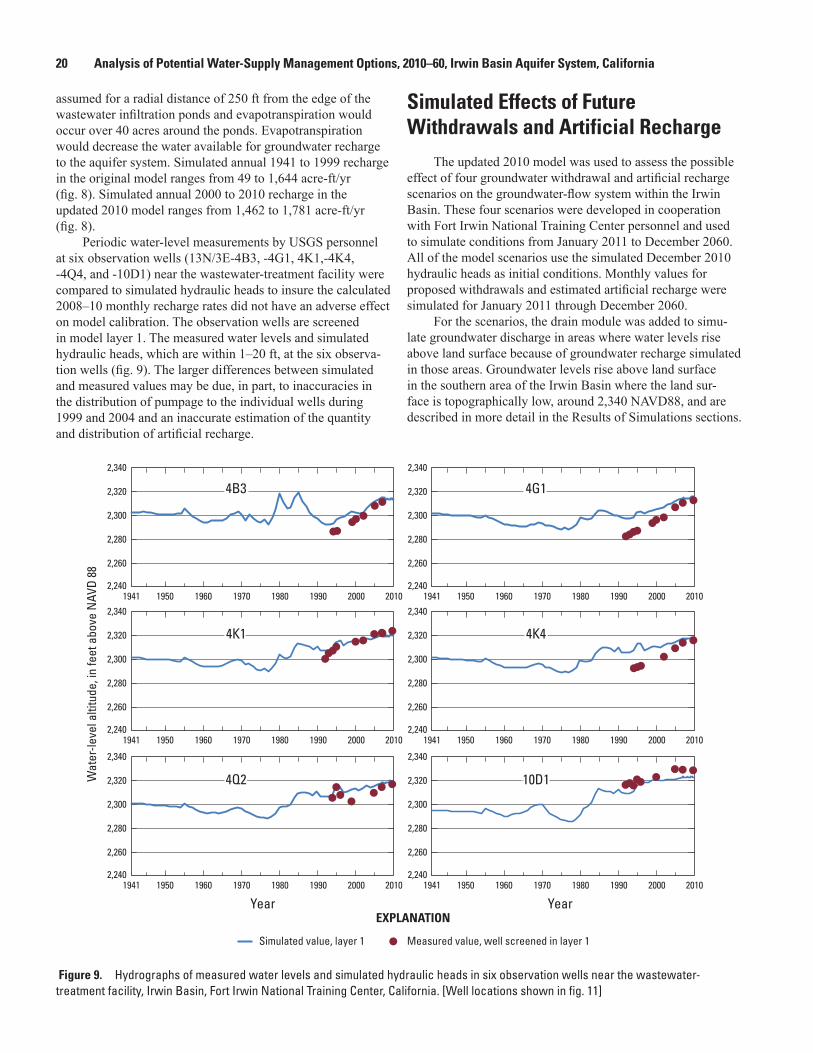
assumed for a radial distance of 250 ft from the edge of the wastewater infiltration ponds and evapotranspiration would occur over 40 acres around the ponds. Evapotranspiration would decrease the water available for groundwater recharge to the aquifer system. Simulated annual 1941 to 1999 recharge in the original model ranges from 49 to 1,644 acre-ft/yr (fig. 8). Simulated annual 2000 to 2010 recharge in the updated 2010 model ranges from 1,462 to 1,781 acre-ft/yr (fig. 8).
Periodic water-level measurements by USGS personnel at six observation wells (13N/3E-4B3, -4G1, 4K1,-4K4, -4Q4, and -10D1) near the wastewater-treatment facility were compared to simulated hydraulic heads to insure the calculated 2008–10 monthly recharge rates did not have an adverse effect on model calibration. The observation wells are screened in model layer 1. The measured water levels and simulated hydraulic heads, which are within 1–20 ft, at the six observa-tion wells (fig. 9). The larger differences between simulated and measured values may be due, in part, to inaccuracies in the distribution of pumpage to the individual wells during 1999 and 2004 and an inaccurate estimation of the quantity and distribution of artificial recharge.
Simulated Effects of Future Withdrawals and Artificial Recharge
The updated 2010 model was used to assess the possible effect of four groundwater withdrawal and artificial recharge scenarios on the groundwater-flow system within the Irwin Basin. These four scenarios were developed in cooperation with Fort Irwin National Training Center personnel and used to simulate conditions from January 2011 to December 2060. All of the model scenarios use the simulated December 2010 hydraulic heads as initial conditions. Monthly values for proposed withdrawals and estimated artificial recharge were simulated for January 2011 through December 2060.
For the scenarios, the drain module was added to simu-late groundwater discharge in areas where water levels rise above land surface because of groundwater recharge simulated in those areas. Groundwater levels rise above land surface in the southern area of the Irwin Basin where the land sur-face is topographically low, around 2,340 NAVD88, and are described in more detail in the Results of Simulations sections.
Figure 9. Hydrographs of measured water levels and simulated hydraulic heads in six observation wells near the wastewater-treatment facility, Irwin Basin, Fort Irwin National Training Center, California. [Well locations shown in fig. 11]
201020001990198019701960195019412,240
2,260
2,280
2,300
2,320
2,340
201020001990198019701960195019412,240
2,260
2,280
2,300
2,320
2,340
201020001990198019701960195019412,240
2,260
2,280
2,300
2,320
2,340
201020001990198019701960195019412,240
2,260
2,280
2,300
2,320
2,340
201020001990198019701960195019412,240
2,260
2,280
2,300
2,320
2,340
201020001990198019701960195019412,240
2,260
2,280
2,300
2,320
2,340
Wat
er-le
vel a
ltitu
de, i
n fe
et a
bove
NAV
D 88
Figure 9. Hydrographs of simulated and measured water levels in 6 observation wells located near the wastewater-treatment facility, Fort Irwin National Training Center, California. (Well location shown in figure 11)
4B34B3 4G14G1
4K14K1 4K44K4
4Q24Q2 10D110D1
EXPLANATION
Simulated value, layer 1 Measured value, well screened in layer 1
YearYear

Simulated Effects of Future Withdrawals and Artificial Recharge 21
Description of Model Scenarios
Artificial groundwater recharge simulated for each of the model scenarios was adjusted in the area of the ponds near the wastewater-treatment facility, based on estimates by Fort Irwin personnel of the quantity of wastewater that may be discharged to the ponds in the future. The quantity of treated wastewater discharged to the ponds is anticipated to be reduced as a result of plans to use the wastewater, rather than “newly pumped” groundwater, for irrigation. Groundwater withdrawals also were adjusted for each of the scenarios to represent the redistribution or reduction of estimated amounts that are anticipated by Fort Irwin personnel. Simulated groundwater withdrawals and artificial recharge for each sce-nario are described below.
Scenario 1Scenario 1 simulates the 2010 annual rate of withdraw-
als (536 acre-ft/yr) from production well 14N/3E-32H1 in the Irwin Basin (table 4) and remains constant from 2011 to 2060. The monthly distribution of withdrawals (fig. 10) was esti-mated as a percentage from the monthly withdrawals from all production wells in the Irwin, Bicycle, and Langford Basins for the 10-year period, 2001 through 2010 in order to reflect the monthly groundwater requirement needed by operations at the Fort Irwin NTC. The monthly groundwater withdrawals for the Irwin Basin were calculated by multiplying the 2010
total groundwater withdrawals (536 acre-ft/yr) from produc-tion well 14N/3E-32H1 by the percentage for a particular month. The monthly withdrawals used in scenario 1 ranged from 27 to 61 acre-ft (table 4).
The estimated quantity of treated wastewater discharged to the infiltration ponds near the wastewater-treatment facil-ity (pond locations shown in fig. 2) for 2011 through 2060 was reduced from the 2010 values. The quantity of treated wastewater discharged to the ponds ranges from 55 to 103 acre-ft/month (table 3) for scenario 1. Because less treated wastewater will be discharged to the ponds, less water will be available for recharge. If the quantity of treated wastewater discharged to the ponds exceeded the total of the evaporation and evapotranspiration rate and was greater than the 2010 monthly recharge rate from the ponds , then the 2010 recharge rate from wastewater shown in table 3 was simulated for that month. If the quantity of treated wastewater discharged to the ponds was less than the total of the evaporation and evapo-transpiration rate and there was wastewater left over from the previous month, then the simulated 2010 recharge rate from wastewater was decreased for that month. If the quantity of treated wastewater discharged to the ponds was less than the total of the evaporation and evapotranspiration rate and there was no wastewater left over from the previous month, then the simulated 2010 recharge rate is zero. The monthly recharge rate in the area of the ponds calculated from the quantity of treated wastewater in the ponds ranged from 0 to 63 acre-ft/month (table 3).
Figure 10. Average 2001 to 2010 total monthly groundwater withdrawal distribution for wells in the Bicycle, Irwin, and Langford Basins that were used to provide water to Fort Irwin National Training Center, California.
0
2
4
6
8
10
12
Jan Feb Mar Apr May June July Aug Sept Oct Nov Dec
Month
Perc
enta
ge o
f ann
ual w
ithdr
awal
s
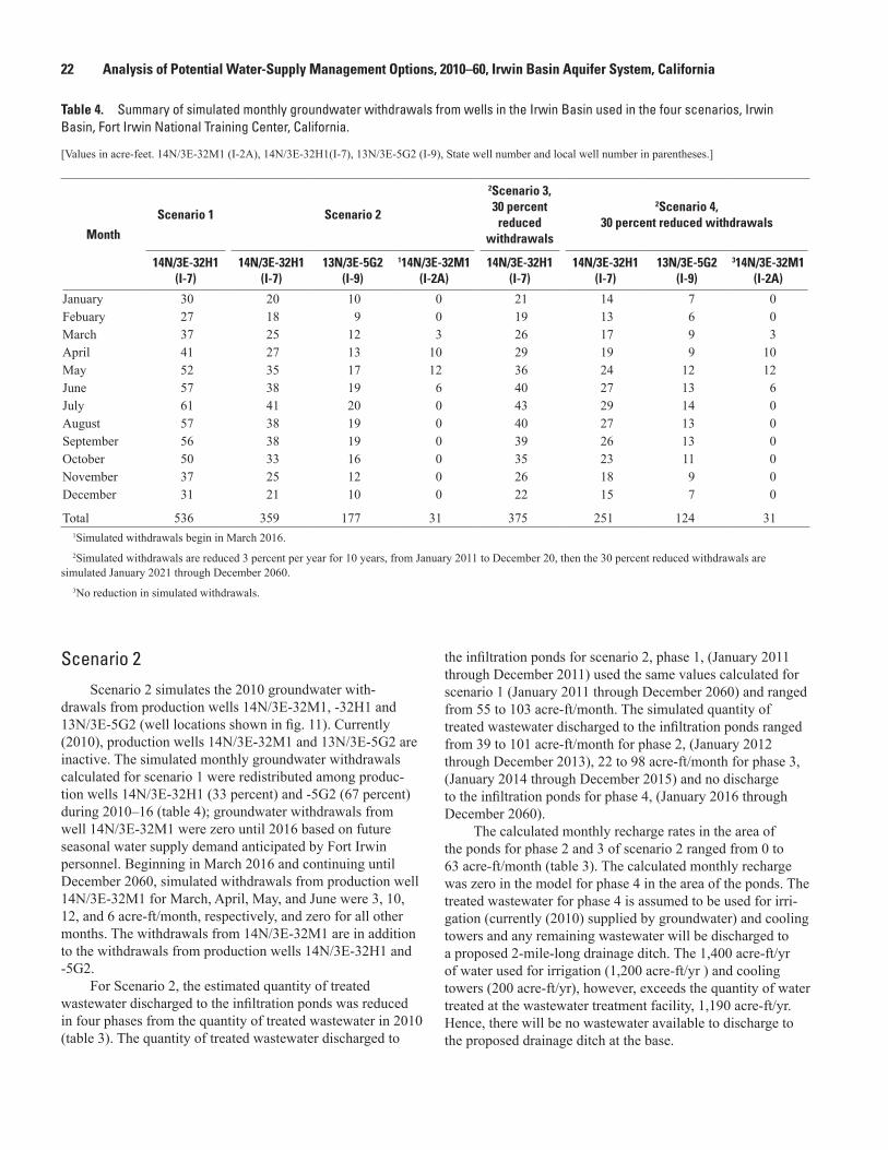
22 Analysis of Potential Water-Supply Management Options, 2010–60, Irwin Basin Aquifer System, California
Scenario 2Scenario 2 simulates the 2010 groundwater with-
drawals from production wells 14N/3E-32M1, -32H1 and 13N/3E-5G2 (well locations shown in fig. 11). Currently (2010), production wells 14N/3E-32M1 and 13N/3E-5G2 are inactive. The simulated monthly groundwater withdrawals calculated for scenario 1 were redistributed among produc-tion wells 14N/3E-32H1 (33 percent) and -5G2 (67 percent) during 2010–16 (table 4); groundwater withdrawals from well 14N/3E-32M1 were zero until 2016 based on future seasonal water supply demand anticipated by Fort Irwin personnel. Beginning in March 2016 and continuing until December 2060, simulated withdrawals from production well 14N/3E-32M1 for March, April, May, and June were 3, 10, 12, and 6 acre-ft/month, respectively, and zero for all other months. The withdrawals from 14N/3E-32M1 are in addition to the withdrawals from production wells 14N/3E-32H1 and -5G2.
For Scenario 2, the estimated quantity of treated wastewater discharged to the infiltration ponds was reduced in four phases from the quantity of treated wastewater in 2010 (table 3). The quantity of treated wastewater discharged to
the infiltration ponds for scenario 2, phase 1, (January 2011 through December 2011) used the same values calculated for scenario 1 (January 2011 through December 2060) and ranged from 55 to 103 acre-ft/month. The simulated quantity of treated wastewater discharged to the infiltration ponds ranged from 39 to 101 acre-ft/month for phase 2, (January 2012 through December 2013), 22 to 98 acre-ft/month for phase 3, (January 2014 through December 2015) and no discharge to the infiltration ponds for phase 4, (January 2016 through December 2060).
The calculated monthly recharge rates in the area of the ponds for phase 2 and 3 of scenario 2 ranged from 0 to 63 acre-ft/month (table 3). The calculated monthly recharge was zero in the model for phase 4 in the area of the ponds. The treated wastewater for phase 4 is assumed to be used for irri-gation (currently (2010) supplied by groundwater) and cooling towers and any remaining wastewater will be discharged to a proposed 2-mile-long drainage ditch. The 1,400 acre-ft/yr of water used for irrigation (1,200 acre-ft/yr ) and cooling towers (200 acre-ft/yr), however, exceeds the quantity of water treated at the wastewater treatment facility, 1,190 acre-ft/yr. Hence, there will be no wastewater available to discharge to the proposed drainage ditch at the base.
Table 4. Summary of simulated monthly groundwater withdrawals from wells in the Irwin Basin used in the four scenarios, Irwin Basin, Fort Irwin National Training Center, California.
[Values in acre-feet. 14N/3E-32M1 (I-2A), 14N/3E-32H1(I-7), 13N/3E-5G2 (I-9), State well number and local well number in parentheses.]
Month
Scenario 1 Scenario 2
2Scenario 3, 30 percent reduced
withdrawals
2Scenario 4, 30 percent reduced withdrawals
14N/3E-32H1 (I-7)
14N/3E-32H1 (I-7)
13N/3E-5G2 (I-9)
114N/3E-32M1 (I-2A)
14N/3E-32H1 (I-7)
14N/3E-32H1 (I-7)
13N/3E-5G2 (I-9)
314N/3E-32M1 (I-2A)
January 30 20 10 0 21 14 7 0Febuary 27 18 9 0 19 13 6 0March 37 25 12 3 26 17 9 3April 41 27 13 10 29 19 9 10May 52 35 17 12 36 24 12 12June 57 38 19 6 40 27 13 6July 61 41 20 0 43 29 14 0August 57 38 19 0 40 27 13 0September 56 38 19 0 39 26 13 0October 50 33 16 0 35 23 11 0November 37 25 12 0 26 18 9 0December 31 21 10 0 22 15 7 0
Total 536 359 177 31 375 251 124 311Simulated withdrawals begin in March 2016.2Simulated withdrawals are reduced 3 percent per year for 10 years, from January 2011 to December 20, then the 30 percent reduced withdrawals are
simulated January 2021 through December 2060.3No reduction in simulated withdrawals.
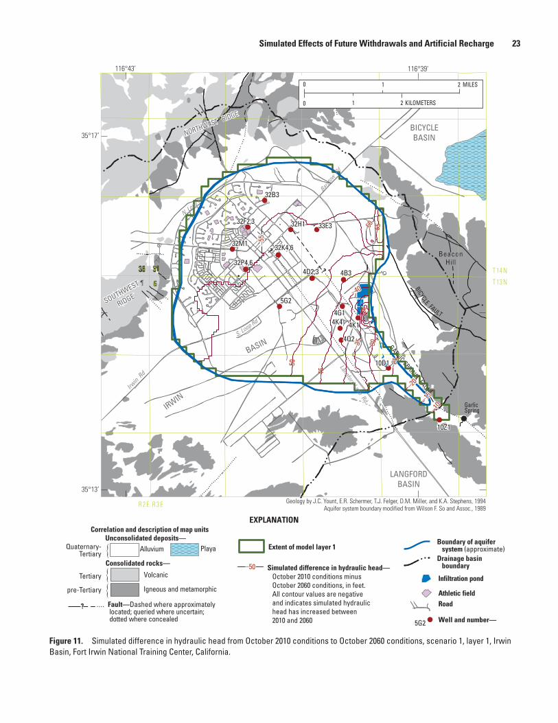
Simulated Effects of Future Withdrawals and Artificial Recharge 23
Figure 11. Simulated difference in hydraulic head from October 2010 conditions to October 2060 conditions, scenario 1, layer 1, Irwin Basin, Fort Irwin National Training Center, California.
LANGFORDBASIN
IRWIN
BASIN
BICYCLEBASIN
BeaconHill
BeaconHill
GARLIC SPRING FAULT
Geology by J.C. Yount, E.R. Schermer, T.J. Felger, D.M. Miller, and K.A. Stephens, 1994Aquifer system boundary modified from Wilson F. So and Assoc., 1989
?
BICYCLE FAULT
?
–55
–50
–45
–40
–35
–30
–60
–15
–10
–25
–20
–65
–25
4D2,3 4B3
4G1
5G2
4K14K4
4Q2
32F2,3 32H1 33E3
32M1 32K4,6
32P4,6
10D1
10Z1
32B3
1
Barsto
w Rd
Irwin R
d
N. Loop Rd
S. Loop Rd
Langford Lake Rd
31
35°17’
35°13’
116°43’ 116°39'
6
36 T 14 N
T 13 N
R 2 E R 3 E
0
0 21 MILES
KILOMETERS21
EXPLANATION
SOUTHWEST
RIDGE
sac13-0507_Figure 11
Unconsolidated deposits—Correlation and description of map units
Quaternary-Tertiary
Consolidated rocks—
Fault—Dashed where approximately located; queried where uncertain; dotted where concealed
Volcanic
Igneous and metamorphic
PlayaAlluvium
?
NORTHWEST RIDGE
GarlicSpring
{{
{Tertiary
pre-Tertiary
Extent of model layer 1
Simulated difference in hydraulic head— October 2010 conditions minus October 2060 conditions, in feet. All contour values are negative and indicates simulated hydraulic head has increased between 2010 and 2060
–50
Road
Infiltration pond
Athletic field
Well and number—5G2
Boundary of aquifer system (approximate)Drainage basin boundary

24 Analysis of Potential Water-Supply Management Options, 2010–60, Irwin Basin Aquifer System, California
Scenario 3Scenario 3 simulates a 3 percent per year reduction in
the 2010 withdrawal rate for 10 years, from January 2011 through December 2020. The 30 percent reduction in with-drawal rate (from the initial 2010 rate) was then applied in the simulation from January 2021 until December 2060 (table 4). The withdrawals are simulated from production well 14N/3E-32H1 (I-7). The same quantity of treated wastewater discharged to the ponds near the wastewater-treatment facility for scenario 1 was used in scenario 3 (table 3). In addition, the same recharge rate simulated in the area of the ponds in scenario 1 was used in scenario 3.
Scenario 4Scenario 4 simulates the same distribution of withdrawals
among the production wells as scenario 2, but reduces the 2010 withdrawals 3 percent per year for 10 years (January 2011 through 2020) at wells 14N/3E-32H1 and 13N/3E-5G2. As in scenario 3, the 30 percent reduction in withdrawal rates (from the initial 2010 rate) was then simu-lated from January 2021 until December 2060 (table 4). With-drawals at well14N/3E-32M1 were not reduced. Similar to scenario 2, the estimated quantity of treated water discharged to the ponds near the wastewater treatment facility and the simulated recharge rate were varied in 4 phases beginning in January 2011, January 2012, January 2014, and January 2016, and are shown in table 3. The same quantity of treated wastewater discharged to the ponds near the wastewater-treat-ment facility for scenario 2 was used in scenario 4. The same recharge rate simulated in the area of the ponds for scenario 2 was used in scenario 4.
Results of Simulations
Results of the simulations of the four scenarios are presented as maps of the difference in hydraulic heads from October 2010 to October 2060 for model layer 1. (figs. 11–14). The head values for October are assumed to represent water levels after the high groundwater withdrawal rates during the summer. A negative value for the change in hydraulic head indicates the simulated hydraulic head has increased between 2010 and 2060.
Hydrographs showing the simulated hydraulic heads for each of the four scenarios from 2011 to 2060 at 14 well locations are presented in figure 15. Water levels in production wells 14N/3E-32M1 (I-2A), -32H1 (I-7) and 13N/3E-5G2 (I-9) are representative of conditions in a cone of depression that may form in response to groundwater withdrawals. The aquifer response in the area of a cone of depression to changes in recharge will be most evident in the hydrographs of production wells. The water levels in observation wells 13N/3E-4D3, -4G1, -4K1, -4K4, -4Q2, -10D1, 14N/3E-32B3, -32F3, -32K6, -32P6, and -33E3 are representative of groundwater conditions in the Irwin Basin. The changes in simulated hydraulic heads at the 14 wells are summarized in table 5.
Scenario 1 In scenario 1, the 2010 annual rate of withdrawals
(536 acre-ft/yr) was held constant from 2011 to 2060, for a cumulative withdrawal of 26,800 acre-ft. Continuation of the 2010 withdrawal rate and recharge from irrigation at the base housing, and a decrease in the recharge at the ponds, resulted in an increase in groundwater levels throughout Irwin Basin. These increases were as much as 55 ft in the area underlying the base housing in the northwestern part of the basin and 10 ft in the southeastern area near the unnamed wash exiting the basin (fig. 11 and table 5). The rise in water levels in the northwestern part of the basin is a result of continued recharge from irrigation at the base housing. Even though there is a simulated decrease in recharge at the ponds, simulated ground-water levels continue to rise in the area of the ponds. Analysis of simulation results indicate groundwater levels rose to land surface around the golf course pond, duck ponds and well 13N/3E-10D1. Simulated groundwater discharge to the drains, which was simulated around the golf course pond, duck ponds and the unnamed wash near well 13N/3E-10D1, ranges from 1 to 205 acre-ft/year by 2060 (table 6). Beginning in March 2044, simulated hydraulic heads rise to land surface at well 13N/3E-10D1 (2,345 ft above sea level [NAVD 88] intermit-tently during the year (fig. 15). Prior to March 2044, simulated hydraulic heads remain below land surface. The altitude of land surface ranges from 2,344ft above sea level [NAVD 88] at well 13N/3E-10D1 to 2,310 ft above sea level [NAVD 88] at well 13N/3E-10Z1. Simulated groundwater levels remained below land surface north and west of the wastewater treatment plant.

Simulated Effects of Future Withdrawals and Artificial Recharge 25
Figure 12. Simulated difference in hydraulic head from October 2010 conditions to October 2060 conditions, scenario 2, layer 1, Irwin Basin, Fort Irwin National Training Center, California.
LANGFORDBASIN
IRWIN
BASIN
BICYCLEBASIN
BeaconHill
BeaconHill
GARLIC SPRING FAULT
Geology by J.C. Yount, E.R. Schermer, T.J. Felger, D.M. Miller, and K.A. Stephens, 1994Aquifer system boundary modified from Wilson F. So and Assoc., 1989
?
BICYCLE FAULT
?
4D2,3 4B3
4G15G2
4K14K4
4Q2
32F2,3 32H1 33E3
32M132K4,6
32P4,6
10D1
10Z1
32B3
1
Barsto
w Rd
Irwin R
d
N. Loop Rd
S. Loop Rd
Langford Lake Rd
31
35°17’
35°13’
116°43’ 116°39'
6
36 T 14 N
T 13 N
R 2 E R 3 E
0
0 21 MILES
KILOMETERS21
EXPLANATION
SOUTHWEST
RIDGE
sac13–0507_Figure 12
Unconsolidated deposits—Correlation and description of map units
Quaternary–Tertiary
Consolidated rocks—
Fault—Dashed where approximately located; queried where uncertain; dotted where concealed
Volcanic
Igneous and metamorphic
PlayaAlluvium
?
NORTHWEST RIDGE
GarlicSpring
{{
{Tertiary
pre-Tertiary
Extent of model layer 1
Simulated difference in hydraulic head— October 2010 conditions minus October 2060 conditions, in feet. All contour values are negative and indicates simulated hydraulic head has increased between 2010 and 2060
Road
Infiltration pond
Athletic field
Well and number—5G2
Boundary of aquifer system (approximate)Drainage basin boundary
–30
–35
–25
–25
–15
–5–4
0
–20
–10
0
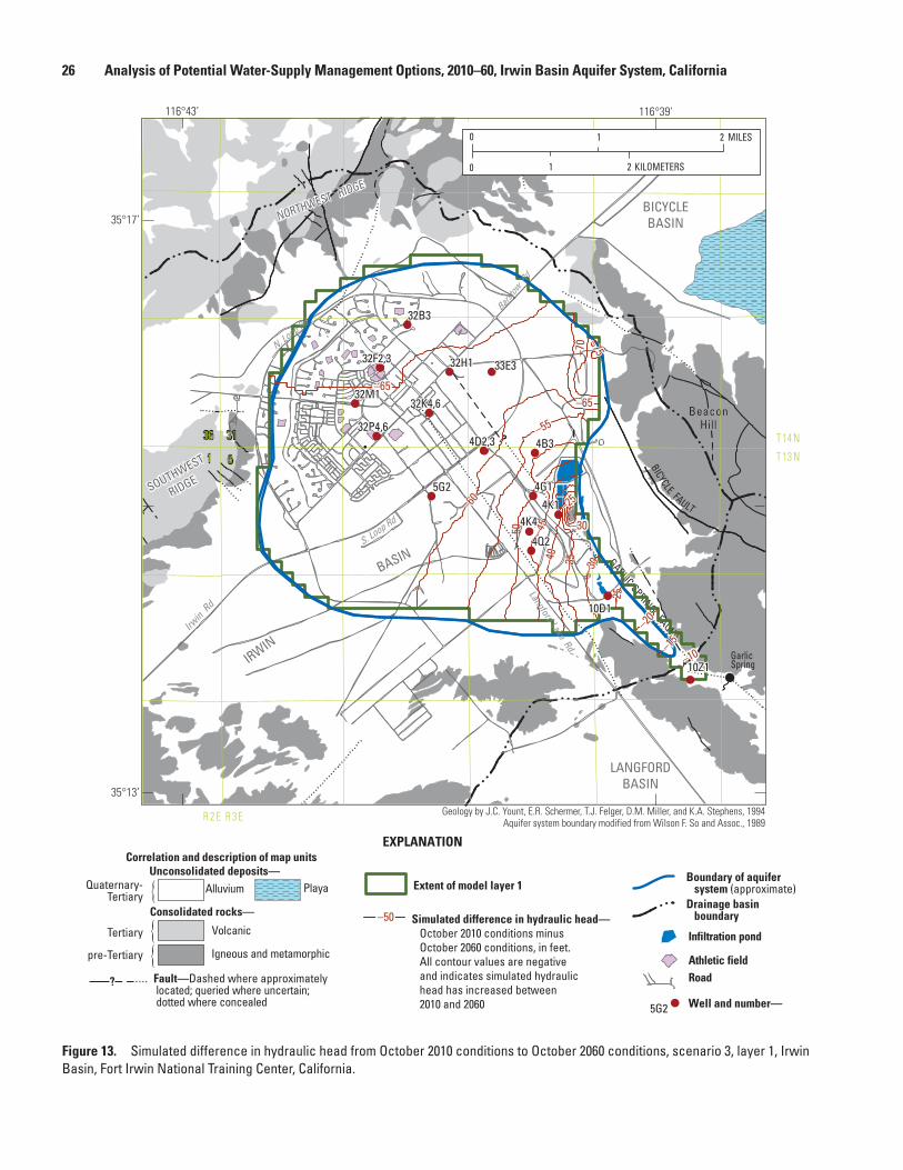
26 Analysis of Potential Water-Supply Management Options, 2010–60, Irwin Basin Aquifer System, California
LANGFORDBASIN
IRWIN
BASIN
BICYCLEBASIN
BeaconHill
BeaconHill
GARLIC SPRING FAULT
Geology by J.C. Yount, E.R. Schermer, T.J. Felger, D.M. Miller, and K.A. Stephens, 1994Aquifer system boundary modified from Wilson F. So and Assoc., 1989
?
BICYCLE FAULT
?–65
–65
–60
–55
–50
–45
–40
–30
–30
–35
–70
–20–15
–25
–10
–75
–25
4D2,3 4B3
4G15G24K1
4K4
4Q2
32F2,3 32H1 33E3
32M132K4,6
32P4,6
10D1
10Z1
32B3
1
Barsto
w Rd
Irwin R
d
N. Loop Rd
S. Loop Rd
Langford Lake Rd
31
35°17’
35°13’
116°43’ 116°39'
6
36 T 14 N
T 13 N
R 2 E R 3 E
0
0 21 MILES
KILOMETERS21
EXPLANATION
SOUTHWEST
RIDGE
sac13-0507_Figure 13
Unconsolidated deposits—Correlation and description of map units
Quaternary-Tertiary
Consolidated rocks—
Fault—Dashed where approximately located; queried where uncertain; dotted where concealed
Volcanic
Igneous and metamorphic
PlayaAlluvium
?
NORTHWEST RIDGE
GarlicSpring
{{
{Tertiary
pre-Tertiary
Extent of model layer 1
Simulated difference in hydraulic head— October 2010 conditions minus October 2060 conditions, in feet. All contour values are negative and indicates simulated hydraulic head has increased between 2010 and 2060
–50
Road
Infiltration pond
Athletic field
Well and number—5G2
Boundary of aquifer system (approximate)Drainage basin boundary
Figure 13. Simulated difference in hydraulic head from October 2010 conditions to October 2060 conditions, scenario 3, layer 1, Irwin Basin, Fort Irwin National Training Center, California.

Simulated Effects of Future Withdrawals and Artificial Recharge 27
LANGFORDBASIN
IRWIN
BASIN
BICYCLEBASIN
BeaconHill
BeaconHill
GARLIC SPRING FAULT
Geology by J.C. Yount, E.R. Schermer, T.J. Felger, D.M. Miller, and K.A. Stephens, 1994Aquifer system boundary modified from Wilson F. So and Assoc., 1989
?
BICYCLE FAULT
?–45
–40
–35
–30
–25 –20 –1
5–5
0
–5
–10
–10
4D2,3 4B3
4G15G2
4K14K4
4Q2
32F2,3 32H1 33E3
32M1 32K4,6
32P4,6
10D1
10Z1
32B3
1
Barsto
w Rd
Irwin R
d
N. Loop Rd
S. Loop Rd
Langford Lake Rd
Road
31
35°17’
35°13’
116°43’ 116°39'
6
36 T 14 N
T 13 N
R 2 E R 3 E
0
0 21 MILES
KILOMETERS21
EXPLANATION
SOUTHWEST
RIDGE
sac13-0507_Figure 14
Unconsolidated deposits—Correlation and description of map units
Quaternary-Tertiary
Consolidated rocks—
Fault—Dashed where approximately located; queried where uncertain; dotted where concealed
Volcanic
Igneous and metamorphic
PlayaAlluvium
?
NORTHWEST RIDGE
GarlicSpring
{{
{Tertiary
pre-Tertiary
Extent of model layer 1
Simulated difference in hydraulic head— October 2010 conditions minus October 2060 conditions, in feet. All contour values are negative and indicates simulated hydraulic head has increased between 2010 and 2060
Infiltration pond
Athletic field
Well and number—5G2
–35
Boundary of aquifer system (approximate)Drainage basin boundary
Figure 14. Simulated difference in hydraulic head from October 2010 conditions to October 2060 conditions, scenario 4, layer 1, Irwin Basin, Fort Irwin National Training Center, California.
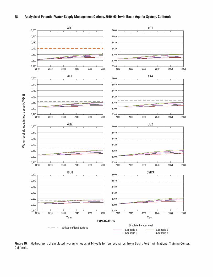
28 Analysis of Potential Water-Supply Management Options, 2010–60, Irwin Basin Aquifer System, California
Figure 15. Hydrographs of simulated hydraulic heads at 14 wells for four scenarios, Irwin Basin, Fort Irwin National Training Center, California.
2,240
2,300
2,360
2,420
2,480
2,540
2,600
2,240
2,300
2,360
2,420
2,480
2,540
2,600
2,240
2,300
2,360
2,420
2,480
2,540
2,600
2,240
2,300
2,360
2,420
2,480
2,540
2,600
2,240
2,300
2,360
2,420
2,480
2,540
2,600
2,240
2,300
2,360
2,420
2,480
2,540
2,600
2,240
2,300
2,360
2,420
2,480
2,540
2,600
2,240
2,300
2,360
2,420
2,480
2,540
2,600
Figure 15 Hydrographs of simulated and measured water levels at 14 wells for four scenarios, Irwin Basin,Fort Irwin National Training Center, California. (Well location shown in figure 11)
206020502010 2020 2030 2040 206020502010 2020 2030 2040
206020502010 2020 2030 2040 206020502010 2020 2030 2040
206020502010 2020 2030 2040 206020502010 2020 2030 2040
206020502010 2020 2030 2040 206020502010 2020 2030 2040
4D3 4G1
4K1 4K4
4Q2 5G2
10D1 32B3
EXPLANATION
Wat
er-le
vel a
ltitu
de, i
n fe
et a
bove
NAV
D 88
Year Year
Simulated water level Altitude of land surface
Scenario 1Scenario 2
Scenario 3Scenario 4

Simulated Effects of Future Withdrawals and Artificial Recharge 29
Figure 15. —Continued
206020502010 2020 2030 2040 206020502010 2020 2030 2040
206020502010 2020 2030 2040 206020502010 2020 2030 2040
206020502010 2020 2030 2040 206020502010 2020 2030 2040
2,240
2,300
2,360
2,420
2,480
2,540
2,600
2,240
2,300
2,360
2,420
2,480
2,540
2,600
2,240
2,300
2,360
2,420
2,480
2,540
2,600
2,240
2,300
2,360
2,420
2,480
2,540
2,600
2,240
2,300
2,360
2,420
2,480
2,540
2,600
2,240
2,300
2,360
2,420
2,480
2,540
2,600
Figure 15-Cont. Hydrographs of simulated and measured water levels at 14 wells for four scenarios,Irwin Basin, Fort Irwin National Training Center, California. (Well location shown in figure 11)
32F3 32H1
32K6 32M1
32P6 33F3
EXPLANATION
Wat
er-le
vel a
ltitu
de, i
n fe
et a
bove
NAV
D 88
Year Year
Simulated water level Altitude of land surface
Scenario 1Scenario 2
Scenario 3Scenario 4
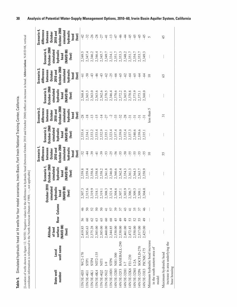
30 Analysis of Potential Water-Supply Management Options, 2010–60, Irwin Basin Aquifer System, CaliforniaTa
ble
5.
Sim
ulat
ed h
ydra
ulic
hea
d at
14
wel
ls fo
r fou
r mod
el s
cena
rios,
Irw
in B
asin
, For
t Irw
in N
atio
nal T
rain
ing
Cent
er, C
alifo
rnia
.
[Loc
atio
n of
wel
ls sh
own
in fi
gure
12.
NO
TE: N
egat
ive
valu
es fo
r the
diff
eren
ce in
hyd
raul
ic h
ead
(bet
wee
n O
ctob
er 2
010
and
Oct
ober
206
0) re
flect
an
incr
ease
in h
ead.
Abb
revi
atio
n: N
AVD
88,
ver
tical
co
ordi
nate
info
rmat
ion
is re
fere
nced
to th
e N
orth
Am
eric
an D
atum
of 1
988;
—, n
ot a
pplic
able
]
Stat
e w
ell
num
ber
Loca
l w
ell n
ame
Alti
tude
of
land
su
rfac
e (N
AVD
88)
(fe
et)
Row
Colu
mn
Oct
ober
201
0 si
mul
ated
hy
drau
lic
head
(N
AVD
88)
(fe
et)
Scen
ario
1,
Oct
ober
206
0 si
mul
ated
hy
drau
lic
head
(N
AVD
88)
(fe
et)
Scen
ario
1,
diffe
renc
e be
twee
n O
ctob
er
2010
and
O
ctob
er 2
060
sim
ulat
ed
hydr
aulic
he
ad
(feet
)
Scen
ario
2,
Oct
ober
206
0 si
mul
ated
hy
drau
lic
head
(N
AVD
88)
(fe
et)
Scen
ario
2,
diffe
renc
e be
twee
n O
ctob
er
2010
and
O
ctob
er 2
060
sim
ulat
ed
hydr
aulic
he
ad
(feet
)
Scen
ario
3,
Oct
ober
206
0 si
mul
ated
hy
drau
lic
head
(N
AVD
88)
(fe
et)
Scen
ario
3,
diffe
renc
e be
twee
n O
ctob
er
2010
and
O
ctob
er 2
060
sim
ulat
ed
hydr
aulic
he
ad
(feet
)
Scen
ario
4,
Oct
ober
206
0 si
mul
ated
hy
drau
lic
head
(N
AVD
88)
(fe
et)
Scen
ario
4,
diffe
renc
e be
twee
n O
ctob
er
2010
and
O
ctob
er 2
060
sim
ulat
ed
hydr
aulic
he
ad
(feet
)
13N
/3E-
4D3
WC
2-17
02,
419.
8556
462,
307.
32,
359.
8–5
22,
335.
4–2
82,
368.
4–6
12,
349.
5–4
213
N/3
E-4G
1ST
P12,
385.
6360
502,
315.
62,
359.
4–4
42,
334.
1–1
82,
365.
3–5
02,
347.
4–3
213
N/3
E-4K
1ST
P42,
375.
2862
522,
319.
92,
358.
6–3
92,
333.
2–1
32,
363.
0–4
32,
346.
2–2
613
N/3
E-4K
4N
IT2-
135
2,38
5.00
6350
2,31
8.1
2,35
8.8
–41
2,33
3.4
–15
2,36
3.6
–46
2,34
6.4
–28
13N
/3E-
4Q2
NIT
12,
385.
0065
502,
319.
12,
358.
2–3
92,
332.
9–1
42,
362.
6–4
32,
345.
7–2
713
N/3
E-5G
2I-
92,
460.
0060
412,
308.
32,
361.
8–5
32,
335.
1–2
72,
370.
5–6
22,
349.
7–4
113
N/3
E-10
D1
STP6
2,34
4.85
6857
2,32
1.4
2,34
6.0
–25
2,32
3.4
–22,
346.
4–2
52,
334.
1–1
314
N/3
E-32
B3
NH
1-30
02,
530.
0045
392,
304.
62,
360.
6–5
62,
337.
4–3
32,
370.
6–6
62,
351.
7–4
714
N/3
E-32
F3B
ASE
BA
LL-2
902,
530.
0049
372,
307.
12,
362.
4–5
52,
339.
0–3
22,
372.
2–6
52,
353.
3–4
614
N/3
E-32
H1
I-7
2,46
1.00
4943
2,30
3.9
2,35
4.3
–50
2,33
2.4
–28
2,36
5.9
–62
2,34
8.2
–44
14N
/3E-
32K
6FI
1-23
02,
472.
4353
412,
306.
72,
361.
3–5
52,
337.
3–3
12,
370.
8–6
42,
351.
7–4
514
N/3
E-32
M1
I-2A
2,55
0.00
5235
2,30
9.3
2,36
4.3
–55
2,34
0.6
–31
2,37
3.9
–65
2,35
4.7
–45
14N
/3E-
32P6
SOC
FLD
-270
2,51
7.00
5537
2,30
9.1
2,36
3.7
–55
2,33
9.6
–31
2,37
3.1
–64
2,35
3.7
–45
14N
/3E-
33E3
PIC
NIC
-175
2,42
5.00
4946
2,30
4.0
2,35
8.9
–55
2,33
5.1
–31
2,36
8.0
–64
2,34
9.3
–45
Min
imum
hyd
raul
ic h
ead
incr
ease
in
the
sout
h ea
ster
n ar
ea o
f m
odel
——
——
—10
—le
ss th
an 5
—10
—5
Max
imum
hyd
raul
ic h
ead
incr
ease
in a
rea
unde
rlyin
g th
e ba
se h
ousi
ng
——
——
—55
—31
—65
—45

Simulated Effects of Future Withdrawals and Artificial Recharge 31
Table 6. Summary of simulated groundwater discharge to drains, Irwin Basin, Fort Irwin National Training Center, California.
[Values in acre-feet.]
Year Scenario 1 Scenario 32011–27 0 0
2028 0 12029 0 32030 0 52031 1 82032 2 112033 3 142034 6 192035 8 232036 10 262037 12 322038 15 392039 19 452040 22 512041 24 602042 28 782043 32 962044 37 1152045 41 1342046 46 1532047 50 1712048 56 1892049 68 2072050 82 2252051 94 2422052 107 2592053 120 2812054 133 3042055 145 3272056 157 3502057 169 3732058 181 3942059 193 4142060 205 432
Scenario 2Scenario 2 simulates the monthly groundwater withdraw-
als that were calculated for scenario 1 distributed initially between two production wells and additional withdrawals later from a third production well. The total volume of simulated groundwater withdrawals was about 28,350 acre-ft in sce-nario 2. Discharge to the wastewater treatment plant used to calculate recharge is estimated to decrease from 2010 values, in 4 phases. The results from the scenario 2 simulation show the least rise in groundwater levels in the Irwin Basin of the four scenarios. Groundwater levels rise about 30 ft near the base housing to less than 5 ft in the unnamed wash exiting Irwin Basin near well 13N/3E-10Z1S (fig. 12 and table 5). Groundwater levels remain below land surface throughout Irwin Basin (fig. 15).
Scenario 3Scenario 3 simulated a reduction of 3 percent per year in
2010 withdrawals from 2011 to 2020 and then held withdraw-als at a constant rate (30 percent less than in 2010) from 2021 to 2060. The total volume of simulated groundwater withdraw-als was reduced from about 26,800 acre-ft in scenario 1 to about 18,760 acre-ft in scenario 3. The reduced recharge rate simulated in scenario 1 was used in scenario 3. The simulated reduction in groundwater withdrawals and recharge rate at the wastewater treatment facility resulted in a rise in groundwater levels throughout the Irwin Basin. Groundwater levels rise 65 ft in the area underlying the base housing in the north-western part of the basin and by 10 ft in the unnamed wash near 13N/3E-10Z1 (fig. 13 and table 5). The results from this scenario show the greatest rise in groundwater levels in the Irwin Basin of the 4 scenarios. Analysis of simulation results indicate groundwater levels will rise to land surface around the golf course pond, duck ponds and well 13N/3E-10D1 (fig. 15). Groundwater discharge to the drains, simulated around the golf course pond, duck ponds and an unnamed wash near well 13N/3E-10D1, ranges from 1 acre-ft/year in 2028 to 432 acre-ft/year by 2060 (table 6).
Scenario 4Scenario 4 simulated a reduction of 3 percent per year
in 2010 withdrawals from 2011 to 2020 distributed among 2 wells, and then a constant rate of withdrawal from 2021 to 2060. Beginning in 2016, an additional withdrawal of 31 acre-ft/yr is simulated from an inactive production well 14N/3E-32M1. The total volume of simulated groundwater withdrawals was about 20,300 acre-ft in scenario 4. The reduced recharge rate simulated in scenario 2 was used in scenario 4. Analysis of results from this simulation indicate groundwater levels rise by 45 ft near the base housing to less than 5 ft in the unnamed wash near 13N/3E-10Z1 (fig. 14). Groundwater levels remain below land surface in the Irwin Basin (fig. 15 and table 5). There is no simulated groundwater discharge to the drains.
Model Limitations
A numerical model is useful for testing and refining a conceptual model of a groundwater flow system, developing an understanding of the system, guiding data collection, and projecting aquifer responses to changes in aquifer stresses within specified limits. However, a model can only approxi-mate the actual system and is based on simplified assump-tions and estimated conditions. Thus, the results of model simulations are only as accurate as the input data and assumed boundary conditions used to constrain the simulations.
32 Analysis of Potential Water-Supply Management Options, 2010–60, Irwin Basin Aquifer System, California
As designed and calibrated, the groundwater-flow model of the Irwin Basin is best used for analyzing basin-wide issues of water use and supply. The model is particularly useful for estimating changes in groundwater levels and flows in the Irwin Basin and flows in response to groundwater withdrawal and artificial recharge. Simulated water levels at locations adjacent to active production wells may not accurately reflect water levels at these locations because simulated water levels are averaged over each model cell and reflect general trends in water levels across a broad area.
Because the model was used to test different quantities and distributions of artificial recharge, the artificial recharge estimates were as representative as possible considering the data limitations. The original model estimated artificial recharge from pumpage data because historical records on the quantities of water used for irrigation and discharged from the wastewater-treatment facility either were not available or may be inaccurate. For the model scenarios, artificial recharge at the wastewater-treatment facility ponds was estimated from 2010 metered data of the quantity of wastewater processed at the wastewater-treatment facility. Estimating artificial recharge in the ponds from the quantity of water processed at the wastewater-treatment facility may be an improvement, but more accurate estimates of artificial recharge quantities and distribution could be used to update and verify the model as they become available. More accurate estimates of artificial recharge from irrigation could be derived if the quantity of water used for irrigation was metered.
Summary and ConclusionsFort Irwin National Training Center presently (2012)
obtains its potable water supply by pumping from wells in the Irwin, Bicycle, and Langford Basins. Groundwater develop-ment began in the Irwin Basin in 1941. Pumping from the Bicycle and Langford Basins began in 1967 and 1992, respec-tively; pumping from these basins has resulted in a decrease in the groundwater demand from the Irwin Basin. Groundwater from Bicycle and Langford basins is imported into the Irwin Basin. Some water is used for irrigation at the base housing; the water that is not consumed is treated at the wastewater-treatment facility and discharged to infiltration ponds. Esti-mated groundwater recharge has exceeded groundwater withdrawals in the Irwin Basin since 1967, except for the years 1984 and 1986–91. From 1967, about 33,980 acre-ft was withdrawn from the groundwater-flow system within the Irwin Basin and an estimated 50,600 acre-ft recharged the basin, resulting in a net gain of 16,620 acre-ft of water to the groundwater-flow system. Reduced pumping in the Irwin Basin, recharge from irrigation at the base housing, and artifi-cial recharge from treated wastewater at the infiltration ponds has caused water levels to stabilize or rise throughout most of the Irwin Basin.
An existing groundwater-flow model of the aquifer system in the Irwin Basin (Densmore, 2003) was updated and used to simulate flow under four alternative withdrawal and recharge conditions, here called scenarios. The updated groundwater-flow model is a useful tool to help estimate the long-term availability of groundwater from the basin by evaluating differences in groundwater-level altitudes (or water levels) among scenarios simulating different withdrawal and recharge rates. The updated model was used to evaluate the potential spatial effects on groundwater levels as a conse-quence of 1) continued withdrawals at the 2010 average rate of pumping, 2) supplementing water-supply needs with with-drawals from an inactive production well, and, 3) a reduction in groundwater recharge from treated wastewater. The four scenarios simulate conditions from January 2011 to December 2060. Scenario 1 simulates the 2010 annual rate of withdrawals (536 acre-ft/yr) from a production well in the Irwin Basin and remains constant from 2011 to 2060. The esti-mated quantity of treated wastewater discharged to the infiltra-tion ponds near the wastewater-treatment facility for 2011 through 2060 was reduced from the 2010 values in scenario 1. Scenario 2 simulates the 2010 annual rate of withdrawals (536 acre-ft/yr) from two production wells in the Irwin Basin until 2060 and additional withdrawals of 31 acre-ft/yr from an inactive well. Discharge to the wastewater treatment plant used to calculate recharge is estimated to decrease from 2010 values, in 4 phases in scenario 2. Scenario 3 simulated a reduction of 3 percent per year in 2010 withdrawals from 2011 to 2020 and then held withdrawals at a constant rate (30 percent less than in 2010) from 2021 to 2060. Scenario 3 uses the same recharge rate simulated in scenario 1. Sce-nario 4 simulated a reduction of 3 percent per year in 2010 withdrawals from 2011 to 2020 distributed among two wells, and then a constant rate of withdrawal from 2021 to 2060. Beginning in 2016, an additional withdrawal of 31 acre-ft/yr is simulated from an inactive production well. The reduced recharge rate simulated in scenario 2 was used in scenario 4.
Analysis of the results from scenario 1 and 3 indicate groundwater levels rise throughout Irwin Basin. These increases were as much as 65 ft in the area underlying the base housing in the northwestern part of the basin and 10 ft in the southeastern area near the unnamed wash exiting the basin. The rise in water levels in the northwestern part of the basin is a result of continued recharge from irrigation at the base housing. Water levels rise to land surface around the golf course pond, duck ponds and in the southeastern area near the unnamed wash exiting the basin. Groundwater discharge to the drains, simulated around the golf course pond, duck ponds and the unnamed wash, ranges from 1 to 432 acre-ft/year by 2060.
The results from the scenario 2 and 4 simulations show the least rise in groundwater levels in the Irwin Basin of the four scenarios. These increases were as much as 45 ft in the area underlying the base housing in the northwestern part of the basin and 5 ft in the southeastern area near the unnamed wash exiting the basin. Groundwater levels remain below land surface throughout the Irwin Basin in scenarios 2 and 4.

References Cited 33
References Cited
California Irrigation Management Information System, 2013, A program in the Office of Water Use Efficiency, California, Department of Water Resources that manages a network of automated weather stations in California: Sacramento, Calif., Department of Water Resources, Office of Water Use Efficiency, accessed on January 24, 2013, http://wwwcimis.water.ca.gov/cimis/myCimis.jsp
Densmore, J.N., 2003, Simulation of groundwater-flow in the Irwin Basin aquifer system, Fort Irwin National Training Center, California: U.S. Geological Survey Water-Resources Investigations Report 02–4264, 69 p.
Densmore, J.N., and Londquist, C.J., 1997, Groundwater hydrology and water quality of Irwin Basin at Fort Irwin National Training Center, California: U.S. Geological Sur-vey Water-Resources Investigations Report 97–4092, 159 p.
EarthInfo, Inc., 1995, National Climatic Data Center summary of the day—West 1994: Boulder, Colo., EarthInfo, Inc., CD-ROM.
EarthInfo, Inc., 2000, EarthInfo CD2 reference manual—for all EarthInfo CD-ROM databases: Boulder, Colo., Earth-Info, Inc., CD-ROM.
Hsieh, P.A., and Freckleton, J.R., 1993, Documentation of a computer program to simulate horizontal-flow barriers using the U.S. Geological Survey modular three-dimensional finite-difference ground-water flow model: U.S. Geological Survey Open-File Report 92–477, 32 p.
Harbaugh, A.W., 2005, MODFLOW-2005, the U.S. Geologi-cal Survey modular ground-water model—the Ground-Water Flow Process: U.S. Geological Survey Techniques and Methods 6-A16, variously paged.
Konikow, L.F., Hornberger, G.Z., Halford, K.J., and Hanson, R.T., 2009, Revised multi-node well (MNW2) package for MODFLOW ground-water flow model: U.S. Geological Survey Techniques and Methods 6-A30, 67 p.
McDonald, M.G., and Harbaugh, A.W., 1988, A modular three-dimensional finite difference groundwater flow model: U.S. Geological Survey Techniques of Water-Resources Investigations, book 6, chap. Al, 586 p.
National Oceanic and Atmospheric Administration, 1994, Climatological data, annual summary, California, 1994: Asheville, N.C., National Oceanic and Atmospheric Admin-istration, v. 98, no. 13.
Wilson F. So and Associates, Inc., 1989, U.S. Army National Training Center at Fort Irwin, California, Water Basin Development Plan, Final Report, June 1989: 85 p.
Wilson, J.D., and Naff, R.L., 2004, The U.S. Geological Sur-vey modular ground-water model—GMG linear equation solver package documentation: U.S. Geological Survey Open-File Report 2004–1261, 47 p.
Yount, J.C., Schermer, E.R., Felger, T.J., Miller, D.M., and Stephens, K.A., 1994, Preliminary geologic map of Fort Irwin Basin, north-central Mojave Desert, California: U.S. Geological Survey Open-File Report 94–173, 27 p.

34 Analysis of Potential Water-Supply Management Options, 2010–60, Irwin Basin Aquifer System, California
This page intentionally left blank.

Prepared by the Sacramento Publishing Service Center.
For more information concerning this report, contact:
DirectorU.S. Geological SurveyCalifornia Water Science Center6000 J Street, Placer HallSacramento, CA [email protected]
or visit our Web site at:http://ca.water.usgs.gov

Voronin and Others—A
nalysis of Potential Water-Supply M
anagement O
ptions, 2010–60, and Docum
entation of Revisions to the Model of the
Irwin B
asin Aquifer System
, Fort Irwin N
ational Training Center, California—Scientific Investigations Report 2014–5081
ISSN 2328-0328
http://dx.doi.org/10.3133/SIR20145081