1

Abstract

In this paper, a model of one-directional propagation of three-component seismic

waves in a nonlinear multilayered soil profile is coupled with a multi-story

multispan frame model to consider, in a simple way, the soil-structure interaction

modelled in a finite element scheme. Modeling the three-component wave

propagation enables the effects of a soil multiaxial stress state to be taken into

account. These reduce soil strength and increase nonlinear effects, compared with

the axial stress state. The simultaneous propagation of three components allows the

prediction of the incident direction of seismic loading at the ground surface and the

analysis of the behavior of a frame structure shaken by a three-component

earthquake.

A parametric study is carried out to characterize the changes in the ground motion

due to dynamic features of the structure, for different incident wavefield properties

and soil nonlinear effects. A seismic response depending on parameters such as the

frequency content of soil and structure and the polarization of seismic waves is

observed.

Keywords: soil-structure interaction, frame, wave propagation, seismic load, finite

element.

1 Introduction

The seismic response of structures depends on ground motion features and on

mechanical properties of structure and soil. The strong ground motion at the surface

of a soil basin, shaking the base of a structure, is also influenced by the dynamic

properties of the structure it-self. The stratigraphy of the soil profile and the

mechanical features of the soil modify the seismic waves, propagating from the

bedrock to the surface, and consequently the seismic loading at the base of

structures. Furthermore, structure oscillation at the soil surface modifies the ground

Analysis of Nonlinear Soil-Structure Interaction Effects

on the response of Three-Dimensional Frame Structures

using a One-Direction Three-Component

Wave Propagation Model

M.P. Santisi d’Avila1

and F. Lopez Caballero2

1Laboratoire J.A. Dieudonné

Université de Nice-Sophia Antipolis, France 2Laboratoire MSS-Mat, CentraleSupélec, Paris, France

2

motion. This effect, known as soil-structure interaction (SSI), is influenced by the

difference in principal frequencies of the soil and structure, due by differences in

terms of mass and stiffness. The wave propagation of an earthquake along a soil

profile, where a free surface is assumed at the top, does not allow take into account

the effects of SSI (Saez et al. [13]).

The research, described in this paper, is directed towards the analysis of the behavior

of a system composed of a frame structure over surface soil layers, under seismic

loading. The one-dimensional (1D) multilayered soil profile is discretized by three-

node line finite elements and a three-dimensional (3D) constitutive relationship

describes the nonlinear soil behavior under cyclic loading. The 3D frame

discretization is performed by using two-node beam finite elements, with six degrees

of freedom per node. Frame structures with shallow foundation, assumed to be rigid,

can be modelled as rigidly connected to the soil at the soil surface, where the three

components of the seismic motion are transmitted from the soil to frame base. The

layered soil system is modelled as primary substructure and the framed structure as

multi-connected secondary substructure, joined at the ground surface level.

The three-component (3C) seismic wave is propagated along a horizontally layered

soil basin from soil-bedrock interface to the ground surface where a multistory

multi-span frame structure is connected. The mutual influence of soil and structure

on their response to seismic loading is studied. Modeling the three-component wave

propagation, the mechanical coupling of multiaxial stress in the soil, inducing

reduced soil strength and increasing nonlinear effects, can be analyzed. The incident

direction of the seismic loading at the ground surface, shaking the frame structure

base, can be taken into account. Different soil properties and soil stratigraphies, with

consequent variation in nonlinear properties and impedance contrast between soil

layers, modify seismic waves by amplification or deamplification effects.

The seismic response of soil profiles can be significantly different in the cases of

free surface and the presence of a structure. The proposed model is a direct solution

method, simultaneously modeling structure and ground motion by a global dynamic

equilibrium equation for the soil-structure system. A one-directional

threecomponent (1D-3C) propagation model (code SWAP_3C by Santisi d’Avila et

al. [14], [15]) is adopted, where the three components of seismic waves are

simultaneously propagated in one direction, from the soil-bedrock interface. An

absorbing condition is assumed at soil-bedrock interface. A nonlinear constitutive

relation of the Masing-Prandtl-Ishlinskii-Iwan type (MPII) is adopted for soil under

multiaxial cyclic loading and a linear behavior is adopted for frame beams. The

model is not dependent on the adopted constitutive relationships.

The three components of seismic motion are evaluated at the base of the 3D frame

structure, taking into account soil nonlinearity, impedance contrast in a multilayered

soil and soil-structure interaction. The ground motion is deduced considering the

impedance contrast between soil and structure, due to their difference in terms of

mass and stiffness.

The proposed 1D-3C propagation model taking into account SSI is implemented in a

code called SFRINT_3C (Soil-FRame INTeraction_3Components).

A parametric analysis is undertaken to observe the effects of SSI for different

combinations of soil features, dynamical properties of structures and earthquake

3

frequency content. Ground motion time histories at the surface, profiles of stress,

strain and motion components with depth and stress-strain hysteresis loops at a fixed

depth are estimated for the soil stratification. Principal frequencies and modal shapes

of the frame structure are evaluated, as well as deformation during the time history.

2 3-Component earthquake propagation in nonlinear soil

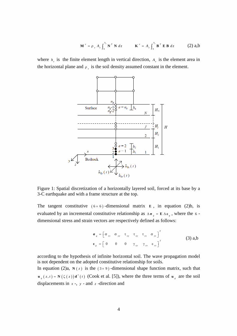
The three components of the seismic motion are propagated into a multilayered

column of nonlinear soil from the top of the underlying elastic bedrock, by using a

finite element scheme. Along the horizontal direction, at a given depth, the soil is

assumed to be a continuous, homogeneous and infinite medium. Soil stratification is

discretized into a system of horizontal layers, parallel to the x y plane, using

quadratic line elements with three nodes (Figure 1). There is not strain variation in

x- and y-direction. Shear and pressure waves propagate vertically in z-direction.

2.1 Spatial discretization

The soil profile is discretized into e

n quadratic line elements and consequently into

2 1g e

n n nodes (Figure 1), having as degrees of freedom the three displacements

in directions x , y and z . Finite element modeling of the horizontally layered soil

system requires spatial discretization, to permit the problem solution, and the

nonlinear mechanical behavior of soil demands time discretization of the process

and linearization of the constitutive behavior in the time step. Accordingly, the

incremental equilibrium equation in dynamic analysis, including compatibility

conditions, three-dimensional constitutive relation and boundary conditions, is

expressed in the matrix form as

g g g g g g g M D C D K D F&& & (1)

where g

D is the assembled 3g

n -dimensional nodal displacement vector of ground,

gD and

gD are the velocity and acceleration vectors, respectively, i.e. the first and

second time derivatives of the displacement vector. g

M and g

K are the assembled

3 3g g

n n -dimensional mass and stiffness matrix, respectively. g

C and g

F are the

assembled 3 3g g

n n -dimensional damping matrix and the 3g

n -dimensional load

vector, respectively, derived from the imposed absorbing boundary condition, as

explained in Section 2.2. The Finite Element Method, as applied in the present

research, is completely described in the works of Batoz and Dhatt [3], Cook et al. [5]

and Reddy [17].

The mass matrix g

M and stiffness matrix g

K result from the assemblage of 9 9 -

dimensional matrices as eM and e

K , respectively, corresponding to the element e ,

which are expressed by

4

0 0

e eh h

e T e T

e e eA d z A d z M N N K B E B (2) a,b

where e

h is the finite element length in vertical direction, e

A is the element area in

the horizontal plane and e

is the soil density assumed constant in the element.

Figure 1: Spatial discretization of a horizontally layered soil, forced at its base by a

3-C earthquake and with a frame structure at the top.

The tangent constitutive 6 6 -dimensional matrix E , in equation (2)b, is

evaluated by an incremental constitutive relationship as g g

σ E ε , where the 6 -

dimensional stress and strain vectors are respectively defined as follows:

0 0 0

T

g xx yy xy zy zx zz

T

g zy zx zz

σ

ε

(3) a,b

according to the hypothesis of infinite horizontal soil. The wave propagation model

is not dependent on the adopted constitutive relationship for soils.

In equation (2)a, zN is the 3 9 -dimensional shape function matrix, such that

,e

gz t z t u N d (Cook et al. [5]), where the three terms of

gu are the soil

displacements in x -, y - and z -direction and

5

2 1 2 1 2 1 2 2 2 2 1 2 1 2 1T

e e e e e e e e e e

x y z x y z x y zu u u u u u u u u

d (4)

is the vector of displacements in directions x , y and z of the three nodes of

element e. Quadratic shape functions, terms of the shape function matrix N ,

corresponding to the three-node line element used to discretize the soil column, are

defined according to Cook et al. [5].

The terms of the 6 9 -dimensional matrix zB , in equation (2)b, are the spatial

derivatives of the shape functions, according to compatibility conditions and to the

hypothesis of no strain variation in the horizontal directions x and y . Given that the

strain vector is related to displacement vector as g g ε u and is a matrix of

differential operators defined in such a way that compatibility equations are verified,

consequently, it is e

gz t ε B d and B N .

The damping matrix eC and load vector e

F in equation (1) depend on boundary

conditions and are defined in Section 2.2.

2.2 Boundary and initial conditions

The system of horizontal soil layers is bounded at the bottom by a semi-infinite

elastic medium representing the seismic bedrock (Figure 2). The following

condition, implemented by Joyner and Chen [11] in a finite difference formulation

and used by Bardet and Tobita [2], is applied at the soil-bedrock interface to take

into account the finite rigidity of the bedrock:

1 02

T p σ c u u& & (5)

The stresses normal to the soil column base at the bedrock interface are Tp σ and c

is a 3 3 -dimensional diagonal matrix whose terms are b sb

v , b sb

v and b p b

v .

The parameters b

, sb

v and p b

v are density, shear and pressure wave velocities in

the bedrock, respectively. According to equation (5), the damping matrix 1C and the

load vector 1F , for the first element 1e , are defined by

1 1

1 1 00 0

2T T

z z

A A

C N c N F N c u& (6) a,b

e

C and eF are a zero-matrix and vector, respectively, for the other elements all over

the soil profile. The three terms of vector 1

u& are the velocities at the soil-bedrock

interface (node 1 in Figure 1) in x -, y - and z -direction, respectively. Terms of the

3 -dimensional vector 0

u& are the input incident velocities, in the underlying elastic

medium, in directions x , y and z , respectively. The 3-Component halved

outcropping bedrock signals 0

u& (Figure 2) are propagated.

6

The absorbing boundary condition (5), assumed at the soil-bedrock interface, allows

energy to be radiated back into the underlying medium. This condition can be easily

modified to use downhole records, assuming an imposed motion at the base of the

soil profile (first node in Figure 1), according to Santisi d’Avila and Semblat [16].

The soil profile is bounded at the bottom by the elastic bedrock and it is connected

to the frame structure at the top. Global equilibrium equation for the soil-frame

system is directly solved, by imposing boundary conditions only at the soil-bedrock

interface.

Gravity load is imposed as static initial condition in terms of strain and stress in each

node.

Figure 2: Representation of seismic signals at different points of the model scheme:

outcropping bedrock, base of the soil profile, free surface at the top of soil profile,

base and top of the frame structure.

2.3 Constitutive model

Modeling the propagation of a three-component earthquake in stratified soils

requires a three-dimensional constitutive model for soil. The so-called Masing-

Prandtl-Ishlinskii-Iwan (MPII) constitutive model, suggested by Iwan [9] and

applied by Joyner [10] and Joyner and Chen [11] in a finite difference formulation,

is used in the present work to properly model the nonlinear soil behavior in a finite

element scheme. The MPII model is used to represent the behavior of materials

satisfying Masing criterion [12] and not depending on the number of loading cycles.

The stress level depends on the strain increment and strain history but not on the

strain rate. This rheological model has no viscous damping. The energy dissipation

process is purely hysteretic and does not depend on the frequency. Iwan [9]

proposes an extension of the standard incremental theory of plasticity (Fung [6]),

modifying the 1D approach by introducing a family of yield surfaces. He models

nonlinear stress-strain curves using a series of mechanical elements, having

different stiffness and increasing sliding resistance. The MPII model takes into

7

account the nonlinear hysteretic behavior of soils in a three-dimensional stress state,

using an elasto-plastic approach with hardening, based on the definition of a series

of nested yield surfaces, according to von Mises’ criterion. The shear modulus is

strain-dependent. The MPII hysteretic model for dry soils, used in the present

research, is applied for strains in the range of stable nonlinearity.

The main feature of the MPII rheological model is that the only necessary input

data, to identify soil properties in the applied constitutive model, is the shear

modulus decay curve G versus shear strain . The initial elastic shear modulus

2

0 sG v , depends on the mass density and the shear wave velocity in the

medium s

v . The P-wave modulus 2

pM v , depending on the pressure wave

velocity in the medium p

v , characterizes the longitudinal behavior of soil.

In the present study the soil behavior is assumed adequately described by a

hyperbolic stress-strain curve (Hardin and Drnevich [7]). This assumption yields a

normalized shear modulus decay curve, used as input curve representing soil

characteristics, expressed as

01 1

rG G (7)

where r

is a reference shear strain provided by test data corresponding to an actual

tangent shear modulus equivalent to 5 0 % of the initial shear modulus. The applied

constitutive model (Iwan [9]; Joyner 1975 [10]; Joyner and Chen 1975 [11]) does

not depend on the hyperbolic backbone curve. It could incorporate also shear

modulus decay curves obtained from laboratory dynamic tests on soil samples.

According to Joyner [10], the actual strain level and the strain and stress values at

the previous time step allow to evaluate the tangent constitutive matrix E in

equation (2) and the stress increment g

σ (Santisi d’Avila et al. [14]).

3 3D frame structure modeling under 3C seismic loading

The response of a regular frame composed by horizontal and vertical beam

elements, along three orthogonal directions x , y and z , shaken by the three

components of a seismic motion, is modelled. Beams are assumed composed by a

continuous and homogeneous medium with constant cross-section along their

longitudinal axis. The hypothesis of plane cross-section, not necessarily

perpendicular to the beam axis, is assumed for beams during deformation. Beam

cross-sectional parameters are the constant area A , the moments of inertia y

I and

zI with respect to y and z axis, respectively, shape factors

y and

z for transverse

shear and the second moment of area J. Material parameters are the compression

modulus E , shear modulus 2 1G E , where is the Poisson’s ratio, and

mass density .

8

3.1 Spatial discretization

The 3D frame structure is modelled by a system of one-dimensional 2-node beam

elements. Each node has 6 degrees of freedom in the x y z global coordinate system,

that are the displacements in x-, y- and z-direction and rotations around the same

axes. The 6-dimensional displacement vector of a generic node in a beam e, parallel

to x -axis, is defined as

T

f x y z x y zu u u

u (8)

The corresponding 6-dimensional vector of nontrivial strains for a 3D beam is

0 0 0T

f xx xz xy

ε (9)

The incremental form of dynamic equilibrium equation of the analyzed 3D frame in

matrix form is

f f f f f f M D C D K D 0 (10)

The dimension of equation (10) is 6fb

n , where fb

n is the number of nodes of the

frame including the base. f

D , f

D and f

D are the 6fb

n -dimensional assembled

vector of nodal displacement, velocity and acceleration, respectively. The consistent

mass matrix f

M , the damping matrix f

C and stiffness matrix f

K are assembled

(Reddy [17]) according to the geometry of the frame. The 6 6fb fb

n n -dimensional

consistent mass matrix f

M and stiffness matrix f

K result from the assemblage of

1 2 1 2 -dimensional matrices as eM and e

K , respectively, of each beam element

e, in global coordinates x y z , which are expressed as (Batoz and Dhatt [3])

e T e e T e

e e e e M Λ M Λ K Λ K Λ (11) a,b

where T

eΛ is the 1 2 1 2 -dimensional rotation matrix, associated to beam e, that

allow to transform displacements and rotations from local coordinates xyz to global

coordinates x y z . eM and e

K , expressed in local coordinates xyz , for a 2-node

beam element e of length Le in x direction, are

0 0

e eL L

e T e TA d x d x M N N K B E B (12) a,b

where A is the beam cross-sectional area and is the material density assumed

9

constant in the element.

A 2-node interdependent interpolation element (Reddy [17]) is used in a finite

element scheme, based on Hermite cubic interpolation of displacements and an

interdependent quadratic interpolation of rotations, so that displacement first

derivative is a polynomial with the same degree of rotations.

The 6 1 2 -dimensional shape function matrix N is defined according to the

transformation ,e

fx t x t u N d , for each beam element e having nodes j

and l, where

TT

e j j j j j j l l l l l l

j l x y z x y z x y z x y zu u u u u u

d d d (13)

is a 12-dimensional time dependent node displacement vector. Shape functions in

matrix N are defined according to Reddy [17]. The 6 1 2 -dimensional matrix B ,

in equation (12)b, is defined in such a way that compatibility equations f f ε u

are verified, where is a matrix of differential operators.

The 6 6 -dimensional constitutive matrix E , in equation (12)b, is defined

according with an incremental constitutive relationship such as f

S E ε , where

T

y z x y zN V V M M M

S (14)

is the vector of internal forces. The frame model is independent from the selected

constitutive law. In this research, a linear behavior for the frame structure material

is assumed, with d iag , , , , ,y z y z

E A G A G A G J E I E I E .

Damping matrix f

C in equation (10) depend on modal analysis and it is defined in

Section 3.3.

3.2 Boundary and initial conditions

The 3D frame is rigidly connected at the ground surface. Consequently, rotations of

the frame base nodes are assumed null.

The shallow foundation is assumed to be rigid. Accordingly, all nodes of the frame

base are supposed to be submitted to the same ground motion.

Static loading configuration represents the initial condition for the frame structure.

The linear elastic solution of static equilibrium equation of the analyzed 3D frame is

f f f

K D F R (15)

where f

F is a 6fb

n -dimensional vector of static nodal loads, obtained by

assembling the 6-dimensional load vectors of frame nodes

10

T

x y z x y zF F F M M M

f (16)

which terms are the external forces directly applied in each node. The 6fb

n -

dimensional vector R is assembled by using the 1 2 -dimensional reaction force

vectors that are e T e

eR Λ R , for each beam e, in global coordinate system. The

terms of vector eR are reaction forces to loads in beam e, expressed in local

coordinates xyz .

3.3 Modal analysis

The system of equations (10) is composed by 6b

n equations related to the motion of

frame base nodes and 6f

n equations corresponding to the motion of the other frame

nodes. Accordingly, equation (10) can be written as

f f f

bb b b f b b b f b b b fb b

tt t

f ffb ff fb ff fb ffff f f

DM M C C K KD D 0

DM M C C K KD D 0

(17)

where f and b indicate each term related with frame and boundary (soil-frame

interface), respectively.

Fundamental fixed-base frequencies of the frame structure are obtained solving the

6f

n -dimensional eigenproblem 2

ff ff K M Φ 0 , where are the natural

angular frequencies and Φ is the modal matrix. The mass-normalization of matrix

Φ implies T

ffΦ M Φ I and

2T

ffΦ K Φ Ω , where 1

d ia g , ...f

n Ω and I is

a 6f

n -dimensional identity matrix.

Damping matrix can be evaluated as 1 1T T

ff f f f f

C Φ Ξ Φ M Φ Ξ Φ M (Chopra

[4]), where 0 0 1 02 d iag 2 , ... , 2

fn

Ξ Ω . The damping ratio 0

is know

for typical materials employed in regular 3D frames. It is assumed 0

0 .0 5 for

typical reinforced concrete buildings. Otherwise, damping matrix can be estimated

by the Rayleigh approach, as 0 1f f f f f f

a a C M K , depending on mass and

stiffness matrices, with 0 0 1 2 1 22a and 1 0 1 2

2a . f

b bC ,

b fC

and fb

C are null.

4 Soil-structure interaction modeling

The 3-Component motion at the base of frame structure is assumed coincident with

ground motion at the top of soil profile (Figure 3). The same loading motion is

applied to all column bases, reducing degrees of freedom of the frame base to only

11

three displacements at the soil-frame interface level ( 6 3b

n ). Rigid rotations of the

foundation are assumed null, supposing that surface waves are negligible, according

to the employed 1D wave propagation model. This analysis considers inertial

interaction modifying the ground motion, due to inertia efforts induced by structure

mass at the soil-structure connection level. Kinematic interaction, induced by

stiffness variation between soil and structure foundation at the most surface soil

layers, is assumed negligible for shallow foundations and vertical propagation.

Figure 3: Spatial discretization of soil (3-node line elements) and frame (2-node

beam elements) with a connection node and elastic boundary condition.

The equilibrium condition under dynamic loading for the soil-frame system is

defined according to the concept of coupling a primary substructure with a multi-

connected secondary substructure, joined at the ground surface level (Figure 1).

Equations (1) can be written as

g g g b g g g b g g g b g g gg g g g

g g g

b g b b b g b b b g b b bb b

M M C C K K D fD D

M M C C K K D 0D D

(18)

indicating with g and b each term related with ground and boundary (interface

between soil and frame), respectively. g

b bC ,

b gC and

g bC are null. The only non-

zero terms in g g

C and g

f are those related to the node at soil-bedrock interface,

according to the adopted boundary condition (see Section 2.2). The total dimension

12

of equation system (18) is 3 6 3g e

n n . It is decomposed in two blocks of 6e

n

equations related to soil motion variables, with e

n the number of finite elements

employed in the soil discretization, and 3 equations associated to ground motion at

the surface.

Equation (17) is rewritten as

f f

bb b b f b b b fb b

tt t

ff f ffb ff fb ffff f f

0 0 DM M K KD D 0

0 C DM M K KD D 0

(19)

considering that f

b bC ,

b fC and

fbC are null (see Section 3.3).

The total dimension of equation system (19) is 6 6 6 3 6fb b f f

n n n n . It is

composed of two blocks of 3 equations related to the motion of frame base,

according to the hypothesis of equal seismic loading at the base of all frame

columns and negligible base rotation, and 6f

n equations corresponding to frame

node motion. A condensation of 6b

n degrees of freedom of base nodes is applied,

allowing to consider only 3 degrees of freedom.

Combining equations (18) and (19), we obtain the following equilibrium equation:

M D C D K D F (20)

where the (6 3 6 ) (6 3 6 )g f g f

n n n n -dimensional mass, damping and

stiffness matrices are, respectively,

g g g b g g g g g b

g f g f

b g b b b b b f b g b b b b b f

fb ff f f fb ff

M M 0 C 0 0 K K 0

M M M M M C 0 0 0 K K K K K

0 M M 0 0 C 0 K K

(21)

The load and displacement increment vectors are, respectively,

T

g

Tt

g g b ff

F f 0 0

D D D D

(22)a,b

The 6f

n -dimensional relative displacement vector of frame nodes is evaluated as

t s

f f f f f f D D D , where

t

f f D is the vector of total displacement increment and

1s

ff f f fb b

D K K D is the displacement vector due to the static application of

base node displacement b

D (Chopra [4]).

13

4.1 Time discretization

Time integration is done according to Newmark’s process. The incremental

dynamic equilibrium equation (20) can be written as

i i i i i

k k k k k k k M D C D K D F (23)

according to time discretization. The subscript k indicates the time step k

t and i

the iteration of the problem solving process. Equation (23) becomes

i i i

k k k k K D F A% (24)

The equivalent stiffness matrix and the equivalent load vector are, respectively,

2

1 1

1

1 1 2 2 1

i i i

k k k k

i i i

k k k k k k k

t t

t t

K M C K

A M C D M C D

%

& &&

(25)a,b

Equation (24) requires an iterative solving, at each time step k , to correct the

tangent stiffness matrix i

kK . Starting from the stiffness matrix 1

1k k K K ,

evaluated at the previous time step, the value of matrix i

kK is updated at each

iteration i . An elastic linear behavior is assumed for the first iteration at the first

time step. The nodal displacement 1

i i

k k k D D D is obtained and strain

increments are deduced from the displacement increments 1

i i

k k k D D D . Stress

increments and the tangent constitutive matrix i

kE are obtained through the

constitutive relationships for the soil. Matrices i

kK , i

kC and the equivalent stiffness

matrix i

kK% are then calculated and the process restarts. The correction process

continues until the difference between two successive approximations is reduced to

a fixed tolerance, according to 1i i i

k k k

D D D , where 3

1 0

.

Total nodal velocity and acceleration are evaluated by

1 1 1

2

1 1 1

1 2

1 1 1 2

i i

k k k k k

i i

k k k k k

t t

t t

D D D D D

D D D D D

& & & &&

&& && & && (26)

Afterwards, the next time step is analyzed. The hypothesis of linear acceleration in

the time step is assumed and the choice of the two parameters 0 .3 0 2 5 and

0 .6 guarantees unconditional stability of the time integration scheme and

numerical damping properties to damp higher modes (Hughes [8]).

14

5 Analysis of the local soil-structure interaction

The influence of 3-Component shaking vs 1C motion and local effects dues to

impedance contrast in multilayered soil are extensively described by Santisi et al.

[14], where the same 1D-3C wave propagation model is used. In this research,

coupling of soil and frame is investigated, to show the interaction effects

reproduced by a one-directional wave propagation model assembled with 3D multi-

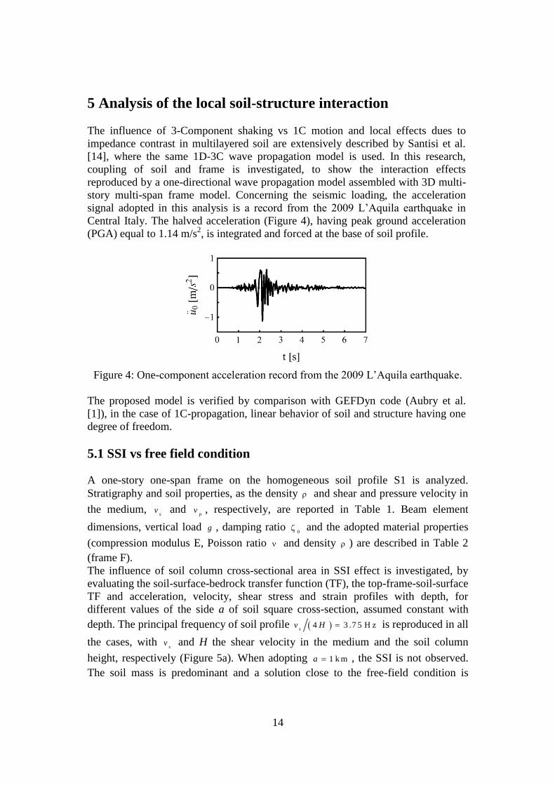
story multi-span frame model. Concerning the seismic loading, the acceleration

signal adopted in this analysis is a record from the 2009 L’Aquila earthquake in

Central Italy. The halved acceleration (Figure 4), having peak ground acceleration

(PGA) equal to 1.14 m/s2, is integrated and forced at the base of soil profile.

Figure 4: One-component acceleration record from the 2009 L’Aquila earthquake.

The proposed model is verified by comparison with GEFDyn code (Aubry et al.

[1]), in the case of 1C-propagation, linear behavior of soil and structure having one

degree of freedom.

5.1 SSI vs free field condition

A one-story one-span frame on the homogeneous soil profile S1 is analyzed.

Stratigraphy and soil properties, as the density and shear and pressure velocity in

the medium, s

v and p

v , respectively, are reported in Table 1. Beam element

dimensions, vertical load g , damping ratio 0

and the adopted material properties

(compression modulus E, Poisson ratio and density ) are described in Table 2

(frame F).

The influence of soil column cross-sectional area in SSI effect is investigated, by

evaluating the soil-surface-bedrock transfer function (TF), the top-frame-soil-surface

TF and acceleration, velocity, shear stress and strain profiles with depth, for

different values of the side a of soil square cross-section, assumed constant with

depth. The principal frequency of soil profile 4 3 .7 5 H zs

v H is reproduced in all

the cases, with s

v and H the shear velocity in the medium and the soil column

height, respectively (Figure 5a). When adopting 1 k ma , the SSI is not observed.

The soil mass is predominant and a solution close to the free-field condition is

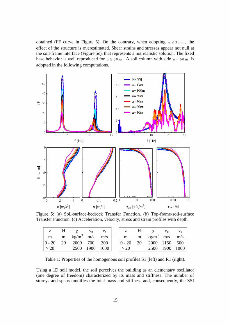
15

obtained (FF curve in Figure 5). On the contrary, when adopting 3 0 ma , the

effect of the structure is overestimated. Shear strains and stresses appear not null at

the soil-frame interface (Figure 5c), that represents a not realistic solution. The fixed

base behavior is well reproduced for 5 0 ma . A soil column with side 5 0 ma is

adopted in the following computations.

Figure 5: (a) Soil-surface-bedrock Transfer Function. (b) Top-frame-soil-surface

Transfer Function. (c) Acceleration, velocity, stress and strain profiles with depth.

z H vp vs

z H vp vs

m m kg/m3 m/s m/s

m m kg/m3 m/s m/s

0 - 20 20 2000 700 300

0 - 20 20 2000 1150 500

> 20 2500 1900 1000

> 20 2500 1900 1000

Table 1: Properties of the homogenous soil profiles S1 (left) and R1 (right).

Using a 1D soil model, the soil perceives the building as an elementary oscillator

(one degree of freedom) characterized by its mass and stiffness. The number of

storeys and spans modifies the total mass and stiffness and, consequently, the SSI

16

effect, but the influence of an increasing floor area, due to an increasing number of

spans, is not captured by a 1D soil model. For this reason, the same soil area is

assumed in all cases in this analysis.

Frame Floors Spans Spans Section L E g 0

x y cm m N/mm2 kg/m

3 kN/m %

F 1 1 1 30x60 3 31220 0.2 2500 13 5

R 3 1 1 40x90 3 31220 0.2 2500 13 5

S 3 1 1 30x50 3 31220 0.2 2500 13 5

T 3 1 1 30x90 3 31220 0.2 2500 13 5

Table 2: Properties of analyzed frame structures.

5.2 Influence of frequency content

The single-frequency Mavroeidis-Papageorgiou wavelet is adopted to study the

effect of frequency content of ground motion, shaking rigid and soft soil profiles,

coupled with rigid and soft frame structures at the top. The outcrop motion is

obtained by the following expression:

0 0 m a x2 1 c o s 2 2 c o s 2 2 0 2

f f fu t u f n t t f t t t t

(27)

where 0 m a x

u , f and 2f

t n f are the acceleration peak, principal frequency and

duration, respectively. The number of peaks is assumed 5n and 2

0 m a x3 .5 mu s .

Acceleration signals are halved to remove the free surface effect and integrated, to

obtain incident velocities, before being forced at the base of the soil profile.

The influence of earthquake frequency content in structural response is analyzed

studying the behavior of a three-story one-span rigid frame R (principal frequency

5 .8 H zf ) shaked by an 1C incident wave having frequency 0

6 H zf , in both

cases of rigid soil R1 ( 6 .2 5 H zg

f ) and softer soil S1 ( 3 .7 5 H zg

f ). This

situation is compared with the behavior of a softer frame S (principal frequency

3 .5 H zf ) shaked by an incident wave having frequency 0

3 .5 H zf , in both

cases of rigid soil R1 and softer soil S1. Beam element dimensions, vertical load g ,

damping ratio 0

and the adopted material properties are described in Table 2 for

the analyzed rigid and softer frame.

This analysis confirms that a rigid frame in a soft soil is less stressed by a seismic

loading having a frequency content close to the frame principal frequency, than in

the case of rigid soil (having principal frequency close to that of frame and quake).

Similarly, a soft frame in a rigid soil is less stressed by a quake having a frequency

content close to the its principal frequency, than in the case of softer soil (having

principal frequency close to that of frame and quake). Numerical results in terms of

horizontal acceleration at the top of the frame structure are showed in Table 3.

17

f (Frame) fg (Soil) f0 (Quake) ü

Hz Hz Hz m/s2

R-R1 5.8 6.25 6.0 8.90

R-S1 5.8 3.75 6.0 4.69

S-S1 3.5 3.75 3.5 20.91

S-R1 3.5 6.25 3.5 12.14

Table 3: Horizontal acceleration at the top of the frame structure.

5.3 Influence of soil nonlinearity

Nonlinear features are characterized, in the adopted MPII constitutive model for

soils, by the shear modulus decay curve. A hyperbolic first loading curve is

assumed and the shear modulus decay curve is defined by Equation (7). The shear

strain r

, related with a 50% decay of shear modulus, is varied to increase

nonlinearity in the multilayered soil profile (Table 4) and observe the associated

effects. The applied incident wave is the 1C signal shown in Figure 4.

Figure 6: (a) Soil-surface-bedrock Transfer Function. (b) Shear stress-shear strain

hysteresis loop. (c) Acceleration, velocity, stress and shear strain profiles with depth.

18

Nonlinear effects lead to strength reduction, strain increasing, and decrement of

principal frequencies (Figure 6). Nonlinear behavior can reduce ground motion

peaks at the ground surface.

z H vp vs

m m kg/m3 m/s m/s

0 - 10 10 1900 539 220

10 - 30 20 1900 980 400

30 - 50 20 1900 1347 550

> 50 1900 2450 1000

Table 4: Properties of a multilayered soil

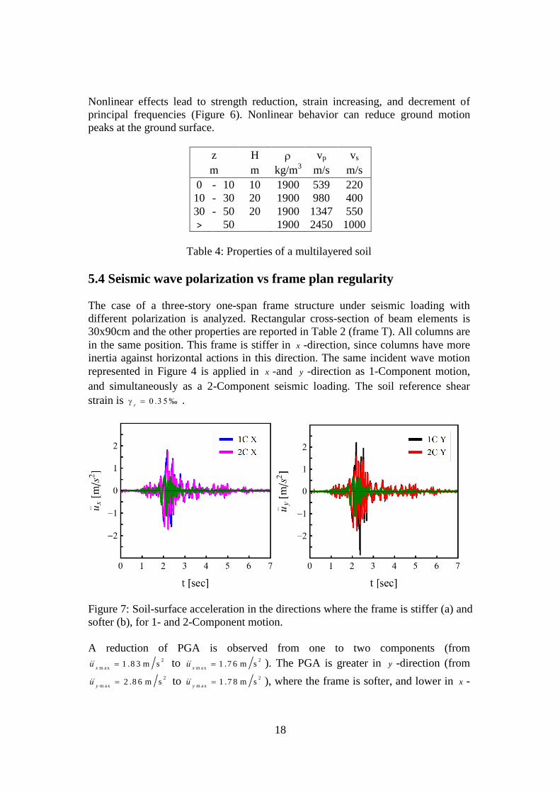
5.4 Seismic wave polarization vs frame plan regularity

The case of a three-story one-span frame structure under seismic loading with

different polarization is analyzed. Rectangular cross-section of beam elements is

30x90cm and the other properties are reported in Table 2 (frame T). All columns are

in the same position. This frame is stiffer in x -direction, since columns have more

inertia against horizontal actions in this direction. The same incident wave motion

represented in Figure 4 is applied in x -and y -direction as 1-Component motion,

and simultaneously as a 2-Component seismic loading. The soil reference shear

strain is 0 .3 5 ‰r

.

Figure 7: Soil-surface acceleration in the directions where the frame is stiffer (a) and

softer (b), for 1- and 2-Component motion.

A reduction of PGA is observed from one to two components (from 2

m a x1 .8 3 m s

xu to 2

m a x1 .7 6 m s

xu ). The PGA is greater in y -direction (from

2

m a x2 .8 6 m s

yu to

2

m a x1 .7 8 m s

yu ), where the frame is softer, and lower in x -

19

direction, where the frame is stiffer. Accelerations at the soil surface and at the top

of the frame structure are lower in the direction where the structure is stiffer.

6 Conclusions

A model of one-directional three-component seismic wave propagation in a

nonlinear multilayered soil profile is coupled with a multi-story multi-span frame

model to consider the soil-structure interaction in a finite element scheme.

Computation time is lower, compared with a 3D spatial discretization of soil and the

boundary condition at the soil-bedrock interface is defined in only one node.

Modeling the simultaneous three-component wave propagation enables the analysis

of the soil multiaxial stress state that reduces the soil strength and increases

nonlinear effects. The variation of incident direction of seismic loading at the

ground surface can be taken into account and the behavior of a frame structure

shaken by a three-component earthquake can be observed.

A sensitivity analysis is carried out to define the appropriate soil column

crosssectional area, allowing to appreciate the Soil-Structure-Interaction effects,

without overestimate the influence of structure. Using a 1D soil model, the soil

perceives the building as an elementary oscillator (one degree of freedom)

characterized by its mass and stiffness. The number of storeys and spans modifies

the total mass and stiffness and, consequently, the SSI effect, but the influence of an

increasing floor area is not captured by a 1D soil model.

Local effects in the soil, dues to nonlinear behavior, impedance contrast between

layers and wavefield polarization, are reproduced by the proposed model. The 3D

model of the frame structure allows to estimate the response to a seismic

acceleration at the base and to evaluate displacement components and internal

forces. A linear behavior is assumed in this analysis for beams, but the proposed

model is not dependent on the adopted constitutive relationship.

This 1D-3C-propagation-3D-frame model allows to confirm that a building is less

stressed by a seismic wave having a frequency content close to the building

principal frequency, if it is placed on a soil with a very different principal

frequency, rather than in the case where soil and structure frequency content are

close together. The acceleration at the soil surface and at the top of a building are

reduced in the direction where the frame structure is stiffer against horizontal

actions.

Further work would require a three-dimensional spatial discretization of soil, to take

into account the influence of building floor area and effects of spatial variability in

the seismic loading.

Acknowledgements

This research has received funding from the European Union's Seventh Framework

Program (FP7/2007-2013) under grant agreement n° 266638 (INTEGER project) as

part of the PEPS Égalité Action (MISS project).

For the second author, a part of the research reported in this paper has been

20

supported by the SEISM Paris Saclay Research Institute.

References

[1] D. Aubry, D. Chouvet, A. Modaressi, H. Modaressi, “GEFDYN: Logiciel

d’Analyse de Comportement Mécanique des Sols par Eléments Finis avec

Prise en Compte du Couplage Sol-Eau-Air”, Scientific Report of Ecole

Centrale Paris, LMSS-Mat, 1986.

[2] J.P. Bardet and T. Tobita, “NERA: A computer program for Nonlinear

Earthquake site Response Analyses of layered soil deposits”, University of

Southern California, United States, 2001.

[3] J.L. Batoz and G. Dhatt, “Modélisation des structures par elements finis”, vol.

2, Hermes Ed, pp.483, 1990.

[4] A.K. Chopra, “Dynamics of structures”, 2nd Ed, Prentice Hall, Upper Saddle

River, New Jersey, pp. 844, 2000.

[5] R.D. Cook, D.S. Malkus, M.E. Plesha and R.J. Witt, “Concepts and

applications of finite element analysis”, 4th Ed, John Wiley and Sons, New

York, United States, pp. 717, 2002.

[6] Y.C. Fung, “Foundation of Soil Mechanics”, Prentice Hall, Englewood Cliffs,

New Jersey, 127-152, 1965.

[7] B.O. Hardin and V.P. Drnevich, “Shear modulus and damping in soil: design

equations and curves”, J. Soil Mech. Found. Div., 98, 667-692, 1972.

[8] T.J.R. Hughes, “The finite element method - Linear static and dynamic finite

element analysis”, Prentice Hall, Englewood Cliffs, New Jersey, pp. 803,

1987.

[9] W.D. Iwan, “On a class of models for the yielding behavior of continuous and

composite systems”, J. Appl. Mech., 34, 612-617, 1967.

[10] W. Joyner, “A method for calculating nonlinear seismic response in two

dimensions”, Bull. Seism. Soc. Am., 65(5), 1337-1357, 1975.

[11] W.B. Joyner and A.T.F. Chen, “Calculation of nonlinear ground response in

earthquakes”, Bull. Seism. Soc. Am., 65(5), 1315-1336, 1975.

[12] S.L. Kramer, “Geotechnical Earthquake Engineering”, Prentice Hall, New

Jersey, 231-248, 1996.

[13] E. Saez, F. Lopez-Caballero and A. Modaressi-Farahmand-Razavi, Effect of

the inelastic dynamic soil-structure interaction on the seismic vulnerability

assessment, Structural Safety, 33(1), 51-63, 2011.

[14] M.P. Santisi d’Avila, L. Lenti and J.F. Semblat, “Modeling strong seismic

ground motion: 3D loading path vs wavefield polarization”, Geophys. J. Int.,

190, 1607-1624, 2012.

[15] M.P. Santisi d’Avila, J.F. Semblat and L. Lenti, “Strong ground motion in the

2011 Tohoku Earthquake: a one-directional three-component modeling”, Bull.

Seism. Soc. Am., Special issue on the 2011 Tohoku Earthquake, 103(2b),

1394-1410, 2013.

[16] M.P. Santisi d'Avila and J.F. Semblat, “Nonlinear seismic response for the

2011 Tohoku earthquake: borehole records versus 1Directional - 3Component

propagation models”, Geophys. J. Int., 197, 566-580, 2014.

21

[17] J.N. Reddy, “An introduction to the Finite Element Method”, 3rd Ed, Mac

Graw Hill ed., pp. 766, 2006.