analysis of non-stationary power quality waveforms using
TRANSCRIPT

University of Wollongong University of Wollongong
Research Online Research Online
University of Wollongong Thesis Collection 1954-2016 University of Wollongong Thesis Collections
2015
Analysis of non-stationary power quality waveforms using iterative Analysis of non-stationary power quality waveforms using iterative
empirical mode decomposition methods and SAX algorithm empirical mode decomposition methods and SAX algorithm
Mohammad Jasa Afroni University of Wollongong
Follow this and additional works at: https://ro.uow.edu.au/theses
University of Wollongong University of Wollongong
Copyright Warning Copyright Warning
You may print or download ONE copy of this document for the purpose of your own research or study. The University
does not authorise you to copy, communicate or otherwise make available electronically to any other person any
copyright material contained on this site.
You are reminded of the following: This work is copyright. Apart from any use permitted under the Copyright Act
1968, no part of this work may be reproduced by any process, nor may any other exclusive right be exercised,
without the permission of the author. Copyright owners are entitled to take legal action against persons who infringe
their copyright. A reproduction of material that is protected by copyright may be a copyright infringement. A court
may impose penalties and award damages in relation to offences and infringements relating to copyright material.
Higher penalties may apply, and higher damages may be awarded, for offences and infringements involving the
conversion of material into digital or electronic form.
Unless otherwise indicated, the views expressed in this thesis are those of the author and do not necessarily Unless otherwise indicated, the views expressed in this thesis are those of the author and do not necessarily
represent the views of the University of Wollongong. represent the views of the University of Wollongong.
Recommended Citation Recommended Citation Afroni, Mohammad Jasa, Analysis of non-stationary power quality waveforms using iterative empirical mode decomposition methods and SAX algorithm, Doctor of Philosophy thesis, School of Electrical, Computer and Telecommunication Engineering, University of Wollongong, 2015. https://ro.uow.edu.au/theses/4482
Research Online is the open access institutional repository for the University of Wollongong. For further information contact the UOW Library: [email protected]

School of Electrical, Computer and Telecommunication Engineering
Analysis of Non-Stationary Power Quality Waveforms
Using Iterative Empirical Mode Decomposition Methods
and SAX Algorithm
Mohammad Jasa Afroni
This thesis is presented as part of the requirements for the
Award of the Degree of the Doctor of Philosophy
University of Wollongong
September, 2015
ii
CERTIFICATION
I, Mohammad Jasa Afroni, declare that this thesis, submitted in partial fulfillment of
the requirements for the award of Ph.D, in the School of Electrical,
Telecommunications and Computer Engineering, University of Wollongong, is
wholly my own work unless otherwise referenced or acknowledge. The document
has not been submitted for qualification at any other academic institution.
Mohammad Jasa Afroni
2 September 2015

iii
ABSTRACT
The nonstationary nature of power-quality (PQ) waveforms requires a tool that can
accurately analyze and visually identify the instants of transitions. One of the
recently reported tools available to analyze nonstationary complex waveforms with a
very good time resolution is the Hilbert Huang Transform (HHT) which consists of
two steps - the Empirical Mode Decomposition (EMD) and the Hilbert Transform
(HT). The EMD process decomposes the signal into Intrinsic Mode Functions
(IMFs), each of which represents the identified signal component. Once the IMFs are
obtained, the HT can then be applied to find the instantaneous amplitude, frequency
and phase of each IMF.
However, HHT has difficulty in resolving waveforms containing components with
close frequencies with a ratio of less than two, and similar to other waveform
classification techniques, it has difficulty in resolving the instants of sudden changes
in the waveform. To overcome the problem with components containing close
frequencies, a novel Iterative Hilbert Huang transform (IHHT) is proposed in this
thesis. The problem in identifying instants of sudden changes in the waveform is
resolved by proposing the use of Symbolic Aggregate ApproXimation (SAX)
method. SAX converts the signal into symbols that can be utilized by a pattern
detector algorithm to identify the boundaries of the stationary signals within a
nonstationary signal. Results from IHHT and SAX method to analyze and visually
identify simulated and measured nonstationary PQ waveforms will be provided and
discussed. The proposed method is particularly useful when investigating the
behavior of the harmonic components of a particular PQ waveform of interest in a
given interval of time, following a data-mining search of a large database of PQ
events. It can be used to both identify, and later isolate unique signatures within a
provider‟s distribution system.
The Hilbert Huang Transform (HHT) can also decompose noisy Power Quality (PQ)
waveforms, however, when the noise level becomes relatively high, the EMD
process may generate mixed IMFs which give inaccurate results when the HT is
applied to the IMFs. To resolve the mode mixing issue, an improved EMD method,
referred to as the Ensemble Empirical Mode Decomposition (EEMD), is then used.
Results from the decomposition process of the signals demonstrate the ability of the
EEMD method in resolving mode-mixing issues resulting from the presence of noise.

iv
However, the EEMD method may not produce accurate instantaneous amplitude
values of the detected IMFs and hence the Iterative EEMD (IEEMD) method is
proposed in this thesis together with the SAX (Symbolic Aggregate approXimation)
based pattern detector algorithm, to determine the boundaries of the segments in the
non-stationary signal. Results from simulated signals show that the proposed
methods are effective in decomposing noisy non-stationary signal.
The Iterative HHT and the Iterative EEMD methods have also been tested with real
single and three phase signals from measurement using Dranetz PQ analyzer and
from Pqube cloud storage of PQ events. The decomposition results have shown the
accuracy of the Iterative HHT over the standard / traditional HHT for less noisy
signals. However, for more noisy signals, the EMD process will fail to identify the
correct frequency of the signal components due to the mode mixing issue and
therefore the standard HHT as well as the iterative HHT can not decompose the
signal accurately. The EEMD method can resolve the mode mixing issue in the
decomposition process of the more noisy signal. However, the MSE of the
reconstructed signal to the original is still high and therefore, the proposed Iterative
EEMD is used to decompose the signals and it is found that the accuracy of the
IEEMD is better than the traditional EEMD method.

v
ACKNOWLEDGEMENTS
I would like to express my sincere gratitude to my supervisor, Prof. Danny Soetanto,
for his guidance and encouragement throughout the duration of my study and the
work of this thesis. Danny has forced me to „understand what is really going on‟ with
each method I employ. His attention to detail is remarkable and quite helpful.
I also wish to thank my co supervisor Dr. David Stirling for guiding me in my study
and the writing of the thesis.
I am very grateful to the Ministry of Education, Directorate General of Higher
Education (DIKTI) Indonesia, for providing me a Ph.D scholarship with sufficient
financial support for me.
I would also like to extend my gratitude to the technical staff of the School of
Electrical, Computer and Telecommunication Engineering (SECTE), particularly
Sean Elphick and Vic Smith for their constant hard work and the pleasant manner in
which they provided solutions to many problems that surfaced during the research.
Special thanks to the students at SECTE, in particular Jan E Alam, Chao Sun, Nishad
Mendis and Hamid Reza Ghasemabadi for all the support and exchange of
knowledge in a very friendly environment.
No list of acknowledgements would be complete without thanking my wife Hariroh
Hannan who has supported me in every way possible. Especially I would like to
acknowledge her patience as I have worked to complete my thesis.
I would also like to thank my children Fayyad, Salsa and Yusuf who has been
patiently spent their time in the home country while I was away for my study.
I also wish to thank my parents and other family members for their unwavering,
never-ending support, inspiration and encouragement in pursuing my education.

vi
Finally, thanks to every friend or family member who has not been mentioned here,
but who have all contributed to making my life easier, more enjoyable and valuable.

vii
TABLE OF CONTENTS
CERTIFICATION ....................................................................................................... ii
ABSTRACT................ ................................................................................................ iii
ACKNOWLEDGEMENTS ......................................................................................... v
TABLE OF CONTENTS.......................................................................................... vii
LIST OF FIGURES .................................................................................................... xi
LIST OF TABLES ................................................................................................... xvii
LIST OF ABBREVIATIONS .................................................................................... xx
CHAPTER 1 INTRODUCTION ............................................................................ 1
1.1. Problem statements and background ............................................................ 1
1.2. Thesis objectives and methodology ............................................................. 3
1.3. Thesis outline ............................................................................................... 4
1.4. Summary of original contributions .............................................................. 5
1.5. Thesis related publications ........................................................................... 5
CHAPTER 2 LITERATURE REVIEW.................................................................. 6
2.1. Introduction .................................................................................................. 6
2.2. Power Quality Problems .............................................................................. 6
2.2.1. Frequency events ...................................................................................... 7
2.2.2. Voltage events .......................................................................................... 7
2.2.3. Waveform Events ..................................................................................... 9
2.3. Effects of PQ Disturbances ........................................................................ 13
2.4. Existing PQ Monitoring Systems ............................................................... 13
2.5. Methods of PQ signal Decomposition ....................................................... 14
2.5.1. Fourier Transform (FT). ......................................................................... 14
2.5.2. Discrete Fourier Transform (DFT) and Fast Fourier Transform (FFT) . 15
2.5.3. Short Term Fourier Transform (STFT) .................................................. 16
2.5.4. Wavelet Transform (WT) ....................................................................... 17
2.5.5. Prony Algorithm .................................................................................... 19
2.5.6. Multiple Signal Classification (MUSIC) ............................................... 21
2.5.7. Estimation of Signal Parameters via Rotational Invariance Techniques
(ESPRIT) .............................................................................................. 24
2.5.8. Hilbert Huang Transform (HHT) ........................................................... 26
2.6. Chapter summary ....................................................................................... 27

viii
CHAPTER 3 The Hilbert Huang Transform (HHT) ............................................. 28
3.1 Introduction ................................................................................................ 28
3.2 Why HHT? ................................................................................................. 28
3.3 The Basic of HHT ...................................................................................... 29
3.3.1 Empirical Mode Decomposition (EMD) ................................................ 29
3.3.2 Hilbert Transform (HT).......................................................................... 40
3.4 Applying HHT to Stationary Signals ......................................................... 47
3.4.1 PQ waveform with harmonics ................................................................ 47
3.4.2 Stationary PQ waveform containing Flicker .......................................... 49
3.5 Applying HHT to Non-Stationary Signals ................................................. 50
3.5.1 Non-stationary PQ waveform with harmonics and sag.......................... 51
3.5.2 Windowing Technique .......................................................................... 52
3.5.3 Non-stationary PQ waveform with harmonics and swell ...................... 53
3.5.4 Non-stationary PQ waveform with transient.......................................... 55
3.6 Issues in implementing HHT ..................................................................... 58
3.6.1 Stopping Criteria .................................................................................... 58
3.6.2 Close Frequency ..................................................................................... 60
3.6.3 Noise ...................................................................................................... 63
3.7 Chapter Summary....................................................................................... 64
CHAPTER 4 METHODS TO IMPROVE HHT ................................................... 65
4.1. Introduction ................................................................................................ 65
4.2. Method to improve HHT using Masking Signal ........................................ 65
4.2.1. EMD using Masking Signal . ................................................................. 65
4.2.2. Results from EMD with Masking Signal ............................................... 68
4.2.3. EMD with Masking Signal and FFT method ........................................ 72
4.2.4. Results from EMD with Masking Signal and FFT method ................... 74
4.3. The proposed Iterative HHT ...................................................................... 80
4.4. Results from the Iterative HHT .................................................................. 83
4.5. Chapter summary ....................................................................................... 89

ix
CHAPTER 5 THE SAX BASED BOUNDARY DETECTOR METHOD AND
ITERATIVE HHT TO DECOMPOSE NON-STATIONARY
SIGNAL .......................................................................................... 92
5.1. Introduction to SAX ................................................................................... 92
5.2. SAX Algorithm .......................................................................................... 92
5.2.1. Applications of SAX .............................................................................. 94
5.2.2. Determination of window size and alphabet size of the SAX
representation ........................................................................................ 98
5.3. The SAX Based Boundary Detector Algorithm....................................... 100
5.4. Applying IHHT and SAX-based Boundary Detector to non-stationary
signals ...................................................................................................... 101
5.4.1. Non-stationary PQ waveform with harmonics variations .................... 101
5.4.2. Non-stationary PQ waveform with harmonics and sag........................ 105
5.4.3. Non-stationary PQ waveform with harmonics and swell .................... 108
5.4.4. Non-stationary PQ waveform with transient........................................ 111
5.5. Chapter summary ..................................................................................... 114
CHAPTER 6 ENSEMBLE EMPIRICAL MODE DECOMPOSITION (EEMD) .
...................................................................................................... 116
6.1. Introduction .............................................................................................. 116
6.2. Standard EEMD Algorithm .................................................................... 117
6.3. The Proposed Iterative EEMD (IEEMD) ................................................. 124
6.4. Results from the Iterative EEMD ............................................................. 126
6.5. Chapter Summary..................................................................................... 128
CHAPTER 7 RESULTS ..................................................................................... 130
7.1. Introduction .............................................................................................. 130
7.2. Measured Signals ..................................................................................... 130
7.2.1. Dranview Signal ................................................................................... 130
7.2.2. PQube Signal ........................................................................................ 132
7.3. The analysis of the stationary measured signals. ..................................... 134
7.3.1. Dranview Signals ................................................................................. 134
7.3.2. PQube Signal ........................................................................................ 145
7.4. Non-stationary signals .............................................................................. 155
7.4.1. Dranview signal ................................................................................... 155

x
7.4.2. PQube signal ........................................................................................ 158
7.5. Chapter summary ..................................................................................... 159
CHAPTER 8 CONCLUSION ............................................................................. 162
8.1. Discussions and Conclusions of the Research Work ............................... 162
8.2. Major contributions .................................................................................. 165
8.3. Future Work ............................................................................................. 166
LIST OF REFERENCES ......................................................................................... 167

xi
LIST OF FIGURES
Figure 2.2.2.1 (a)Voltage sag and swell (b) Voltage unbalance. ............................... 8
Figure 2.2.2.2 Voltage fluctuations............................................................................. 8
Figure 2.2.2.3 Voltage interruption............................................................................. 8
Figure 2.2.3.1 Harmonic. ............................................................................................ 9
Figure 2.2.3.2 Inter-harmonic.................................................................................... 9
Figure 2.2.3.3 Notching. ........................................................................................... 10
Figure 2.2.3.4 Typical transients (a) from lightning (b) from system switching ..... 10
Figure 2.2.3.5 A waveform with noise content. ....................................................... 11
Figure 3.3.1.1 The Flowchart of EMD process..........................................................31
Figure 3.3.1.2 The components of signal S(t), (a) 50Hz component (b) 150 Hz
component (c) The signal S(t) ............................................................................ 32
Figure 3.3.1.3 The signal with identified maxima and minima................................. 32
Figure 3.3.1.4 The signal with maximum and minimum envelopes......................... 33
Figure 3.3.1.5 The signal with identified mean envelope.......................................... 33
Figure 3.3.1.6 The waveform of a(t) superimposed on Figure 3.3.1.5...................... 34
Figure 3.3.1.7 The waveform of σ (t) superimposed on Figure 3.3.1.6..................... 34
Figure 3.3.1.8 The waveform of m1 superimposed on Figure 3.3.1.7. ..................... 35
Figure 3.3.1.9 The new S(t) with the local mean....................................................... 36
Figure 3.3.1.10 The evaluation of Cmean(t) ................................................................ 36
Figure 3.3.1.11 The new S(t) with the local mean..................................................... 37
Figure 3.3.1.12 The evaluation of Cmean(t)................................................................ 37
Figure 3.3.1.13 The first residue of the signal S(t) .................................................. 38
Figure 3.3.1.14 The new S(t) with the local mean................................................... 38
Figure 3.3.1.15 The evaluation of Cmean(t)................................................................ 39
Figure 3.3.1.16 The second residue of the process................................................... 39
Figure 3.3.1.17 The Final result of Empirical Mode Decomposition process on S(t),
(a) The signal S(t), (b) IMF1 (150Hz), (c) IMF2 (50Hz)..................................... 40
Figure 3.3.2.1 The Hilbert Transform of S(t). ...........................................................41
Figure 3.3.2.2 The instantaneous amplitude of S(t). ................................................. 42
Figure 3.3.2.3 The analytic signal z(t) of IMF2 obtained by the Hilbert Transform.. 42
Figure 3.3.2.4 The instantaneous amplitude of IMF2. ............................................ 43
Figure 3.3.2.5 The instantaneous phase angle of S(t). .............................................. 43

xii
Figure 3.3.2.6 The instantaneous phase angle of S(t) after the subtraction. ............. 44
Figure 3.3.2.7 The instantaneous Frequency of S(t). ................................................ 44
Figure 3.3.2.8 The instantaneous Frequency of IMF2. ............................................ 45
Figure 3.3.2.9 The instantaneous phase angle of IMF2. .......................................... 46
Figure 3.3.2.10 The Hilbert Transform applied on a multicomponent signal. (a) The
multi-component signal (b) Instantaneous frequency (c) Instantaneous
Amplitude.......................................................................................................... 46
Figure 3.4.1.1 The EMD process of S(t)................................................................... 47
Figure 3.4.1.2 The instantaneous frequency, amplitude and phase of the detected
IMFs of S(t). (a) IMF1, (b) IMF2, (c) IMF3.............................................................. 48
Figure 3.4.2.1 The EMD process of a signal S(t) containing flicker, (a) The signal
S(t), (b) IMF1...................................................................................................... 49
Figure 3.4.2.2 The Hilbert Transform to obtain instantaneous frequency, amplitude
and phase angle of (a) The signal contains Flicker (b) The flicker signal.......... 50
Figure 3.5.1.1 The EMD process on a signal SA(t) with harmonic and sag. (a) The
Signal SA(t) (b) IMF1 (c) IMF2........................................................................ 51
Figure 3.5.1.2 The result from Hilbert Transform of SA(t): (a) Instantaneous
Amplitude, (b) Instantaneous frequency (c) Instantaneous Phase...................... 51
Figure 3.5.2.1 The result from windowing technique on SA(t): (a) Instantaneous
Amplitude, (b) Instantaneous frequency (c) Instantaneous Phase...................... 53
Figure 3.5.3.1 The EMD process of signal SB(t) with harmonic and swell (a) The
Signal SB(t) (b) IMF1 (c) IMF2............................................................................. 54
Figure 3.5.3.2 The result from Hilbert Transform of SB(t): (a) Instantaneous
Amplitude, (b) Instantaneous frequency (c) Instantaneous Phase...................... 54
Figure 3.5.3.3 The result from windowing technique of signal SB(t): (a)
Instantaneous Amplitude, (b) Instantaneous frequency (c) Instantaneous
Phase................................................................................................................... 55
Figure 3.5.4.1 The signal SC(t) contains transient..................................................... 56
Figure 3.5.4.2 The resulting IMFs of a transient signal SC(t).....................................56
Figure 3.5.4.3 The Hilbert Transform of IMFs of SC(t): (a) IMF1, (b) IMF2, (c)
IMF3................................................................................................................... 56
Figure 3.5.4.4 The result from windowing technique of signal SC(t): (a) IMF1, (b)
IMF2, (c) IMF3.................................................................................................... 57

xiii
Figure 3.6.2.1 EMD process on a signal that contains close frequency (a) The signal
S(t), (b) IMF1, (c) IMF2..................................................................................... 61
Figure 3.6.2.2 Hilbert Transform of the IMFs from EMD process on a signal that
contains close frequency (a) IMF1, (b) IMF2...................................................... 62
Figure 3.6.3.1 EMD process of a signal that contains noise, (a) The Signal S(t) (b)
IMF1, (c) IMF2, (d) IMF3, (e) IMF4, (e) IMF5..................................................... 63
Figure 4.2.1.1 The result of Standard EMD and EMD with masking signal (a) The
original signal x(t) (b) The result without masking signal (c) The result with
masking signal................................................................................................... 67
Figure 4.2.2.1 The original X1(t) and the IMFs obtained from EMD process of
X1(t)`................................................................................................................... 68
Figure 4.2.2.2 The Hilbert Transform of IMF1 of X1(t)........................................... 69
Figure 4.2.2.3 The EMD process using masking signal, a) IMF+ , b) IMF- ........... 70
Figure 4.2.2.4 a) The average of IMF+ and IMF- , b) inst. amplitude, c) inst.
frequency, d) inst. phase............................................................................... 70
Figure 4.2.2.5 The original signal X1(t), IMF1 and the residue after iteration 1..... 71
Figure 4.2.2.6 The EMD with masking signal process of X1(t)................................ 71
Figure 4.2.4.1 The EMD process using masking signal and FFT at iteration 1 (k=3)
a) IMF+ , b) IMF- .............................................................................................. 74
Figure 4.2.4.2 a) The average of IMF+ and IMF- for k=3, b) inst. amplitude,
c) inst. frequency, d) inst. phase.............................................................. 75
Figure 4.2.4.3 The original signal X1(t), reconstructed signal, and the residue........ 77
Figure 4.4.1 The first IMF from iteration 1 of the IHHT process on X1(t)............... 83
Figure 4.4.2 The first IMF from iteration 2 of the IHHT process on X1(t)............... 84
Figure 4.4.3 The first IMF from iteration 1 of the IHHT process on X2(t)............. 85
Figure 4.4.4 The first IMF from iteration 2 of the IHHT process on X2(t)............. 86
Figure 5.1.1 The process to discretize the time series or signal (thin black line) to
obtain a PAA approximation (heavy gray line) and then to convert the PAA
coefficients into symbols (bold letters) by using the predetermined breakpoints.
In the example above, with n = 224, w = 32 and a = 3, the signal is mapped to a
word-size of 7 SAX representation “cbaabcb”................................................... 93
Figure 5.2.1.1.1 The second IMF of the start-up current for a) healthy machine, b) a
machine with one broken bar and c) a machine with two broken bars.............. 94
xiv
Figure 5.2.1.1.2 IMF2 of the start up current and the SAX representation............ 95
Figure 5.2.1.1.3 The distance matrix of normal and faulty signal......................... 95
Figure 5.2.1.3.1 An ECG signal with 3 detected anomalies (discords)which exactly
coincides with the heart anomaly....................................................................... 97
Figure 5.2.1.3.2 Detection of unusual voltage profile............................................ 97
Figure 5.2.2.1 SAX representations of signal S(t) with alphabet size = 50 (a) Using
window size w = 20 (b). Using window size w = 40.......................................... 98
Figure 5.2.2.2 SAX representation of a noisy signal using w = 5............................. 99
Figure 5.2.2.3 SAX representation of a noisy signal using w = 10....................... 100
Figure 5.4.1.1 A Non-stationary signal with harmonics variations Sk(t)................ 102
Figure 5.4.1.2 the SAX representation of a non-stationary signal Sk(t) with harmonic
variations.......................................................................................................... 103
Figure 5.4.2.1 Non-stationary signal with harmonics and sag SL(t)........................ 106
Figure 5.4.2.2 SAX representation of SL(t)............................................................. 106
Figure 5.4.3.1 The original signal SM(t)................................................................... 109
Figure 5.4.3.2 The SAX representation of signal SM(t).......................................... 109
Figure 5.4.4.1 The original signal SN(t).................................................................. 111
Figure 5.4.4.2 The instantaneous frequency plot of IMF1 of SN(t)......................... 112
Figure 5.4.4.3 The SAX representation of the instantaneous frequency data of IMF1
from EMD process of SN(t).............................................................................. 112
Figure 6.1.1 Two types of mixed IMFs, a) Uniformly mixed IMF, b) Intermittently
mixed IMF......................................................................................................... 116
Figure 6.2.1 The EMD process of S(t).................................................................... 118
Figure 6.2.2 The noisy signal S1(t)...........................................................................118
Figure 6.2.3 The results of standard EMD on a noisy signal S1(t) (a) IMF1 (b) IMF2
(c) IMF3 (d) IMF4 (e) IMF5............................................................................. 119
Figure 6.2.4 IMFs3 obtained from 10 times EMD process of S1(t), x and y in
denote the IMF set (1 to 10), and the IMF number (here 3) from each set
respectively. Red line in each IMF plot indicates the instantaneous amplitude,
while the dashed black line indicates the mean of instantaneous amplitude
obtained from HT............................................................................................. 122

xv
Figure 6.2.5 The Hilbert Transform of the averaged IMFs3 shown in Figure 6.2.4
(a)The averaged IMFs3 (b) The instantaneous frequency (c) The instantaneous
amplitude (d) The instantaneous phase angle................................................... 123
Figure 7.2.1.1 Dranetz Power Xplorer PX5 power quality Analyzer (source: Davis
Instruments).............................................................................................. 131
Figure 7.2.1.2 Connection Diagram of a PQ Analyzer for Current
Measurement..................................................................................................... 131
Figure 7.2.1.3 The measured signals at various measurement time a).
Dranview#062, b). Dranview#214, c). Dranview#265, d).
Dranview#427................................................................................................... 132
Figure 7.2.2.1 PQube DRK-270-00 PQ analyzer device (source:
jsdata)................................................................................................................. 133
Figure 7.2.2.2 Pqube signal a) GMC-I signal, b) IMH signal ................................ 134
Figure 7.3.1.1 The IMFs obtained from the EMD process of Dranview
Event#062.......................................................................................................... 135
Figure 7.3.1.2 Final result of HHT process of Dranview Event#062; the original
signal, the reconstructed signal and the residue................................................ 136
Figure 7.3.1.3 The IMFs obtained from the EMD process of Dranview Event#062
iteration 2.......................................................................................................... 137
Figure 7.3.1.4 The Hilbert Transform of IMF4 shown in Figure 7.3.1.3(e)............ 138
Figure 7.3.1.5 The Final Result of Iterative HHT process of Dranview
Event#062......................................................................................................... 139
Figure 7.3.1.6 The result of EMD on Dranview#214.............................................. 140
Figure 7.3.1.7 The Hilbert Transform of the IMFs from EMD process on
Dranview#214.................................................................................................. 141
Figure 7.3.1.8 The resulting IMFs from the EEMD process of Dranview#214
signal................................................................................................................. 142
Figure 7.3.1.9 The Hilbert Transform of the IMFs from EEMD process of
Dranview#214................................................................................................... 143
Figure 7.3.1.10 Final result of IEEMD process of DranviewEvent#214................ 144
Figure 7.3.2.1 The IMFs obtained from EMD process of Pqube signal................. 145
Figure 7.3.2.2 The Hilbert Transform of the IMFs from EMD process of Pqube
signal................................................................................................................. 146

xvi
Figure 7.3.2.3 The IMFs obtained from EMD process of Pqube signal
Iteration 2......................................................................................................... 147
Figure 7.3.2.4 The Hilbert Transform of IMF3, IMF4, IMF5, IMF6 and IMF7 from
Iterative HHT process of Pqube signal at iteration 2........................................ 148
Figure 7.3.2.5 EEMD process of Pqube signal........................................................ 149
Figure 7.3.2.6 The Hilbert Transform of the IMFs in Figure 7.3.2.5...................... 150
Figure 7.3.2.7 The IMFs from IEEMD process of Pqube signal iteration 2............ 151
Figure 7.3.2.8 The Hilbert Transform of the IMFs in Figure 7.3.2.7..................... 153
Figure 7.3.2.9 The Final result of Iterative EEMD process on Pqube signal......... 154
Figure 7.4.1.1 A SAX representation of non-stationary Dranview
signal................................................................................................................. 155
Figure 7.4.1.2 Final result of the Iterative EEMD on non-stationary Dranview
signal................................................................................................................. 157
Figure 7.4.2.1 The PQube voltage sag signal......................................................... 158
Figure 7.4.2.2 Final Result of IEEMD on the connected PQube signal: (a) The
original signal (b) IMF1 (c) IMF2, (d) Residue (e) Phasor Diagram of 50 Hz
IMF................................................................................................................... 159
xvii
LIST OF TABLES
Table 2.1 PQ Disturbances....................................................................................... 12
Table 2.2 Typical Effects of voltage Events. ........................................................... 13
Table 2.3 Typical Effects of Waveform Events....................................................... 13
Table 3.1 The result of The Hilbert Transform of the IMFs of S(t).......................... 48
Table 3.2 The Hilbert Transform of IMFs of Flicker signal...................................... 50
Table 3.3 The result from windowing technique and HHT of SA(t).......................... 53
Table 3.4 Result from windowing technique and HHT of SB(t)............................... 55
Table 3.5 The result from HHT and windowing technique of a transient signal
SC(t)....................................................................................................................... 57
Table 3.6 Result of HHT decomposition of the signal S(t) Using θ1= 0.05, θ2 = 0.5
and tol = 0.05....................................................................................................... 59
Table 3.7 Result of HHT decomposition of the signal S(t) using θ1= 0.0005,
θ2 = 0.005 and tol = 0.0005.................................................................................. 59
Table 3.8 Result of HHT decomposition of the signal S(t) using θ1= 5.10-11
,
θ2 = 5.10-10
, tol = 5.10-11
and MAXITERATION = 5.105..................................
60
Table 3.9 Result of HHT decomposition of the signal S(t)........................................62
Table 3.10 The Hilbert Transform of the IMFs from EMD process of signal S(t) in
(3-20)..................................................................................................................... 64
Table 4.1 Result of HHT decomposition of the signal X1(t)...................................... 68
Table 4.2 The results of HT of the IMFs from EMD process of X1(t)...........................72
Table 4.3 The calculated masking signals..................................................................74
Table 4.4 The result of demodulation process of IMF from iteration 1, k=3............. 76
Table 4.5 The result of demodulation process of IMF from iteration 2, k=2............. 76
Table 4.6 The residue after iteration 1....................................................................... 77
Table 4.7 The result of EMD with Masking Signal and FFT method........................78
Table 4.8 The Final result of EMD with Masking Signal and FFT method.............. 78
Table 4.9 The result of EMD with masking signal and FFT on X2(t)........................ 79
Table 4.10 The Final result of EMD with masking signal and FFT on X2(t).............79
Table 4.11 The HT of IMF1 at iteration 1.................................................................. 83
Table 4.12 The HT of IMF1 in the iteration 2........................................................... 84
Table 4.13 The result of IHHT process on X1(t)........................................................ 85
Table 4.14 Final result of IHHT process on X1(t)...................................................... 85

xviii
Table 4.15 The HT of IMF1 at iteration 1...................................................................86
Table 4.16 The HT of IMF1 at iteration 2.................................................................. 86
Table 4.17 The result of IHHT process on X2(t)....................................................... 87
Table 4.18 Final result of IHHT process on X2(t)...................................................... 87
Table 4.19 Separation of Harmonic Signals using standard HHT............................ 88
Table 4.20 Separation of Harmonic Signals using Iterative HHT............................. 89
Table 5.1 A lookup table that contains the breakpoints that divides a Gaussian
distribution from 3 to 5 of equiprobable regions.................................................. 93
Table 5.2 The SAX word for two consecutive cycles of Signal Sk(t)...................... 104
Table 5.3 Result of HHT decomposition of Signal Sk(t).......................................... 105
Table 5.4 Result of IHHT decomposition of Signal Sk(t)........................................ 105
Table 5.5 The SAX word for two consecutive cycles of Signal SL(t)...................... 107
Table 5.6 Result of HHT decomposition of signal SL(t).......................................... 108
Table 5.7 Result of IHHT decomposition of signal SL(t)........................................ 108
Table 5.8 The SAX word for two consecutive cycles of Signal SM(t)..................... 110
Table 5.9 Result of HHT decomposition of signal SM(t)......................................... 110
Table 5.10 Result of IHHT decomposition of signal SM(t)...................................... 111
Table 5.11 The SAX word for two consecutive segments of Signal SN(t).............. 113
Table 5.12 Result of HHT decomposition of signal SN(t)........................................ 114
Table 5.13 Result of IHHT decomposition of signal SN(t)...................................... 114
Table 6.1 The HT of the IMFs obtained by EMD of S1(t)...................................... 119
Table 6.2 The calculated mean value of the amplitude of each IMF....................... 122
Table 6.3 The result of EEMD process on S1(t).......................................................124
Table 6.4 The detected components of noisy signal S1(t) using IEEMD.................127
Table 6.5 The Final Result of IEEMD process on noisy signal S1(t).......................127
Table 6.6 The MSE of the decomposition results using IEEMD and EEMD......... 128
Table 7.1 The Measurement time of Various Dranview Signals............................ 133
Table 7.2 The HT results of IMFs from EMD process of Dranview
Event#062............................................................................................................ 136
Table 7.3 The HT results of IMFs from IHHT process of Dranview Event#062
iteration 2............................................................................................................ 138
Table 7.4 Final Result of IHHT process on Dranview Event#062 signal............... 139
Table 7.5 The HT of the IMFs from EMD process on Dranview#214.................... 140

xix
Table 7.6 Hilbert Transform of the IMFs from the EEMD process of Dranview#214
signal................................................................................................................... 142
Table 7.7 The HT of the IMFs from IEEMD process of Dranview#214................ 144
Table 7.8 Final Result of IEEMD process of Dranview#214................................. 144
Table 7.9 The HT of the IMFs from EMD process of Pqube signal........................146
Table 7.10 The Hilbert Transform of IMFs from IHHT process of Pqube signal
iteration 2............................................................................................................. 148
Table 7.11 The HT of IMFs from EEMD process of Pqube signal......................... 150
Table 7.12 The Hilbert Transform of the IMFs in Figure 7.3.2.7............................ 152
Table 7.13. The result of the Hilbert Transform of the IMFs from Pqube signal.... 154
Table 7.14. The final result of the IEEMD process of Pqube signal....................... 154
Table 7.15 The SAX word for two consecutive cycles of non-stationary Dranview
signal.................................................................................................................... 156
Table 7.16 Result of EEMD decomposition of non-stationary Dranview signal.... 156
Table 7.17 Result of IEEMD decomposition of non-stationary Dranview signal... 157
Table 7.18 The detected boundaries of PQube signal.............................................. 158
xx
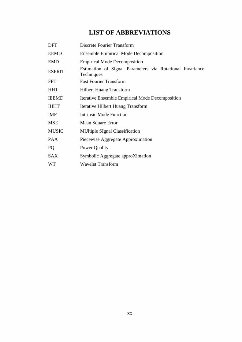
LIST OF ABBREVIATIONS
DFT Discrete Fourier Transform
EEMD Ensemble Empirical Mode Decomposition
EMD Empirical Mode Decomposition
ESPRIT Estimation of Signal Parameters via Rotational Invariance
Techniques
FFT Fast Fourier Transform
HHT Hilbert Huang Transform
IEEMD Iterative Ensemble Empirical Mode Decomposition
IHHT Iterative Hilbert Huang Transform
IMF Intrinsic Mode Function
MSE Mean Square Error
MUSIC MUltiple SIgnal Classification
PAA Piecewise Aggregate Approximation
PQ Power Quality
SAX Symbolic Aggregate approXimation
WT Wavelet Transform
1
CHAPTER 1 INTRODUCTION
1.1. Problem statements and background
The growth of the usage of power electronics equipment at the customer side,
such as computers and consumer electronics, right through to adjustable-speed drives
has become the source of Power Quality (PQ) pollution which will create poor PQ
environment. At the same time, the use of sensitive electrical equipment controlled
by power electronics or microprocessor is rapidly increasing. When there is no
balance of the PQ environment with the immunity characteristics of the sensitive
equipment, many PQ problems may occur which may lead to reduced reliability and
expensive outages at the customer side [1].
In a competitive electricity market, electricity utilities are required to guarantee
the operation of the customer‟s equipment by providing a high quality power supply
in order to satisfy their customer. To meet both utility and customer requirements,
continuous monitoring of PQ waveforms is essential.
Most of PQ waveforms are non-stationary and noisy in nature which requires a
tool that can accurately analyse and visually identify the components of various PQ
events. Fourier Transform (FT) is a simple and computationally efficient algorithm
which has dominated the data analysis work since it was first discovered. However,
there are some crucial limitations of the Fourier spectral analysis: the data must be
strictly stationary and the system must be linear; otherwise, erroneous resulting
spectrum will be obtained [2]. Since most PQ events are usually non-stationary, the
Short-Time Fourier Transform (STFT) has been developed to analyze such signals.
A windowing technique is used by the STFT method to concentrate the FT on a
smaller area of the entire signal [3]. However, the width of the window needs to be
fixed prior to carrying out the analysis. Therefore, the resolution of the STFT method
is fixed, which may not produce accurate result when the signal being analyzed
contains various frequencies.
Wavelet Transform (WT) uses flexible windowing function which is shifted
and scaled version of the mother wavelet. Therefore, Wavelet analysis can give good
time resolution for high-frequency events, and good frequency resolution for low-
frequency events. However, once the mother function has been chosen, it will have
to be used to analyze all of the data, which may require a different choice of mother

2
wavelet because of the non-stationary nature of the signal. The WT is therefore not
adaptive to analyze the on-stationary PQ waveforms [2].
A couple of parametric methods such as Prony analysis, Multiple Signal
Classification (MUSIC) and Estimation of Signal Parameters via Rotational
Invariance Techniques (ESPRIT) have also been used for PQ signal analysis. The
parametric methods estimate the signal parameters (such as amplitude, frequency and
phase) by fitting the signal being analyzed to the model used in the method. It is
reported that parametric methods are very accurate to estimate the signals parameters
[4]. However, the methods assume that the number of sinusoids in the signal are
known prior to the analysis which may not be possible for most practical cases [4].
One of the recently reported tools available to analyse non-stationary complex
waveforms with a very good time resolution is the Hilbert Huang Transform (HHT)
which consists of two distinct processes. First the signal to be analyzed is
decomposed using the Empirical Mode Decomposition (EMD) process into Intrinsic
Mode Functions (IMFs) that have meaningful instantaneous frequencies, amplitudes
and phases of the signal components being analyzed [5]. Second, The Hilbert
Transform is then applied to each IMF giving the instantaneous amplitude, frequency
and phase versus time. HHT method does not require any assumption before the
analysis and hence it can be considered as an adaptive method. However, it has been
reported [6], [7], that the HHT has difficulties in decomposing harmonic signals
containing close frequencies that occasionally results in IMFs with mixed
frequencies. Mixed IMFs generally produce incorrect result from the Hilbert
Transform and therefore they are not desirable. The IMFs with mixed frequencies are
also found, when the signal being analyzed by the EMD process contain relatively
significant noise level [8].
The EMD process estimates the local average of the waveform being analyzed
by identifying the maxima and minima points of the waveform which are then
connected by using cubic spline interpolation to build the maxima and minima
envelopes. The local average is approximated from the mean of these envelopes.
However, since the points to be interpolated are not sufficiently available at both
ends of the waveform, the end effect phenomenon generally appears in the resulted
IMF, which is another issue with the EMD method [2].
3
1.2. Thesis objectives and methodology
The aim of this thesis is to develop a methodical approach using the original
and the extended Hilbert Huang Transform, Ensemble Empirical Mode
Decomposition and SAX boundary detector to decompose non-stationary PQ signals
that contain close frequency components and noise. The decomposition result can
assist data analysts or utility engineers to analyse the monitored data. Such approach
will also allow the utility engineers to gain more information into the occurrence of
PQ events that may damage electrical equipment.
Although various researchers have endeavoured to address mode mixing
problem resulted from the EMD process of signals containing close frequencies,
none has exploited the mixed IMF resulting from the original EMD process. The new
concept proposed in this thesis is based on utilising certain IMFs (which may be
mixed) produced by the original EMD, that contain correct mean value of
instantaneous frequencies, and subtracting these from the original signal. The HHT
process is then repeated in an iterative mode (so that all signal components are
decomposed accurately), in contrast to subtracting all IMFs obtained from a typical
HHT process at once. The proposed technique which is referred to as the Iterative
HHT, modifies the IMFs to sinusoidal representations by using the mean values of
amplitude, frequency and phase obtained from the Hilbert Transform of the IMFs.
Therefore, the end effect issue is avoided by using such technique.
Ensemble EMD (EEMD) which has been proposed by Wu [9], is a variant of
EMD where an ensemble of white noise-added signals is created from the original
data. The EMD is applied to each of these signals to produce an ensemble of IMFs
which are then averaged to obtain the final IMF. EEMD has been recently reported to
help in solving some of the issues with mode mixing [9] resulting from the EMD
process of noisy signals [8]. However, the results from the EEMD method has been
found to produce inaccurate amplitude values of the components since the averaging
process of the mixed IMFs may produce final identified amplitudes which are less
than the actual values. This inaccuracy indicates that part of the signal components
remain unidentified by the decomposition process [8]. Therefore, a similar iterative
technique to the HHT improvement is proposed in this thesis to obtain the remaining
signal component in the residue. The sinusoidal representations of the IMFs are also
used in the Iterative EEMD method to avoid the end effect issue.

4
Both the Iterative HHT and Iterative EEMD use EMD algorithm as the main
method to perform the decomposition process. The EMD process is employed in an
iterative fashion to improve the accuracy of the decomposition process of the
proposed methods. These methods are therefore referred to as the Iterative EMD
techniques in the thesis.
To analyze non-stationary signals, Symbolic Aggregate ApproXimation (SAX)
algorithm is used in the thesis to obtain a symbolic representation of the signal which
is then used by a boundary detector algorithm to identify the instant of changes of the
signal. The identified instant of changes are then used to segment the signal to a
sequence of stationary signals The decomposition methods are then applied to
decompose the signal of the associated segment.
In summary, the objectives of the thesis are as follows:
1. To investigate the application of HHT techniques to decompose PQ events.
2. To extend the HHT technique to remove mode mixing issues when used to
decompose PQ events containing closely related frequencies.
3. To investigate the application of the EEMD technique in decomposing noisy
PQ events.
4. To adapt the EEMD technique to mitigate mode mixing issues when used to
decompose more noisy PQ events
5. To develop a signal pre-processing method by using a SAX-based boundary
detector to identify the boundaries of non-stationary signals so that the
decomposition method can be used for the analysis of non-stationary signals.
1.3. Thesis outline
The outline of the thesis is as follows. Chapter 2 will provide the literature
review. Chapter 3 will introduce the HHT method and discuss the issue in
implementing HHT. Chapter 4 will describe several techniques from the literature to
improve the HHT method in resolving the mode mixing problem caused by signals
having close frequency components. A new method using an iterative process will
also be proposed to improve the original HHT in decomposing such signals. Chapter
5 will present a signal pre-processing technique to identify the boundaries of the non-
stationary signal by translating the signal to a lower dimensional representation using
SAX algorithm and applying a boundary detector to the symbolic representation of
the original data. Chapter 6 will describe the traditional Ensemble Empirical Mode

5
Decomposition (EEMD) and propose the Iterative Ensemble Empirical Mode
Decomposition (IEEMD) to improve its accuracy. Chapter 7 will provide the results
of the application of the decomposition methods to measured signals. A summary of
the thesis and a discussion of future work are contained in Chapter 8.
1.4. Summary of original contributions
The following methods are the original contributions of the research.
1. The development of the Iterative Hilbert Huang Transform.
2. The development of the Iterative Ensemble Empirical Mode Decomposition.
3. The development of SAX-based boundary detector to identify the instant of
changes of the non-stationary signal.
1.5. Thesis related publications
The following publications have been the result of the research presented in the
thesis:
Journal papers
AFRONI, M. J., SUTANTO, D. & STIRLING, D. 2013 “Analysis of Non-Stationary
Power Quality Waveforms Using Iterative Hilbert Huang Transform and SAX
Algorithm” IEEE Transactions on Power Delivery 28, 2134 - 2144.
Conference and presentation
AFRONI, M. J., SUTANTO, D. & STIRLING, D. “SAX-based decomposition of
non-stationary Power Quality waveforms”. In: Harmonics and Quality of
Power (ICHQP), 2012 IEEE 15th International Conference on, 2012. IEEE,
829-834.
AFRONI, M. J., & SUTANTO, D. "The Hilbert Huang Transform for decomposition
of Power Quality waveforms,". In Power Engineering Conference (AUPEC),
2014 Australasian Universities, 2014, pp. 1-6.

6
CHAPTER 2 LITERATURE REVIEW
2.1. Introduction
PQ disturbances due to the usage of power electronics equipment may cause
harmful effect such as malfunction or failure to sensitive power electronic and
microprocessor controlled equipments. To get the consumers satisfaction, the electric
utilities need to maintain good PQ supply in such a competitive electricity market
nowadays. Therefore, PQ monitoring and PQ troubleshooting are becoming more
important to the electric utilities to ensure a high level of service [10].
This chapter initially describes the increasing PQ problems and why PQ
monitoring is needed. A review of the techniques that have been used to analyse PQ
data obtained from such monitoring system is then presented. The basics of signal
processing techniques such as Fourier Transform (FT), Discrete Fourier Transform
(DFT), Short Term Fourier Transform (STFT), Wavelet Transform (WT), Prony
Algorithm, Multiple Signal Classification (MUSIC), and Estimation of Signal
Parameters via Rotational Invariance Techniques (ESPRIT) which can be used to
analyze PQ events are discussed. Finally the use of Hilbert Huang Transform is
presented. The advantage and limitation of each technique is discussed.
2.2. Power Quality Problems
The increasing use of power electronics equipment has polluted the power
system with harmful PQ disturbances such as harmonics input current which consist
not only a power frequency component, which can be 50 Hz or 60Hz, but also
harmonic components which may cause overheating of induction motors and
transformers [10]. Other PQ events such as over-voltage, under-voltage, sag and
swell has also been reported to significantly contribute to the pollution of the PQ
environment [10], [11]. When there is no balance of PQ environment with the
immunity characteristics of the equipment, PQ disturbances may cause malfunction
or damage to the electrical equipment which lead to reduced reliability and expensive
outages [1].
For a deeper understanding of PQ issues, it is important to understand the
basics of PQ [12]. PQ has been defined as "a set of electrical boundaries that allow
equipment to function in its intended manner without significant loss of performance
or life expectancy" [13] and "any power problems manifested in voltage, current or

7
frequency deviation that result in failure or mal-operation of customer equipment,"
[14]. Therefore, to have sufficient understanding of PQ, it is necessary to study the
deviation of the load current, the supply voltage, or the frequency waveforms from
the pure sinusoidal waveforms [12]. Chowdhury reported that voltage disturbances
(such as voltage sags) can result in malfunction of equipment that can cost
approximately 20 billion dollars annually in the United States [15].
There are three general types of PQ disturbances that may be experienced by a
power system, as follows [11]:
a) Frequency events.
b) Voltage events.
c) Waveform events.
The above events will be described in more details in the following
subsections.
2.2.1. Frequency events
The frequency of power system is usually determined by the rotational speed
of generators in the power station. The stability of the power system interconnection
and the efforts made to maintain the frequency within the required limits make
frequency deviations beyond the acceptable range to be a very rare phenomenon
[16]. Therefore, this type of event will not be discussed further in the thesis.
2.2.2. Voltage events
In Australia, the supply voltage is normally held in the range +10% and -6% at
the customer‟s point of connection which is considered as the normal PQ range [17].
If the supply voltage rises much higher than the rated voltage (over-voltage) or
decreases lower than the rated voltage (under-voltage), PQ problems may occur. For
example, over-voltage causes overstressed motor insulation while under-voltage may
cause motor overheating which can lead to loss of life [11].

8
Voltage variations can be divided into the following categories [11]:
a) Long term variations of duration more than 1 minute. These are called over-
voltage (if greater than 110% of nominal voltage) or under-voltage (if less than
90% of nominal voltage).
b) Short term variations lasting less than 1 minute. These are called swell (voltage
greater than 110% of nominal) or sag (voltage between 10% and 90% of
nominal). These are illustrated in Figure 2.2.2.1(a).
c) Voltage unbalance where the voltage of each phase conductor is different to
other phases as shown in Figure 2.2.2.1(b).
Figure 2.2.2.1. (a)Voltage sag and swell (b) Voltage unbalance.
d) Voltage fluctuations is continuous or random fluctuations in the amplitude of
the supply voltage that can be observed as light flicker as shown by Figure
2.2.2.2.
Figure 2.2.2.2. Voltage fluctuations
e) Voltage Interruption is a complete lost of the supply voltage. The voltage
interruption waveform is shown in Figure 2.2.2.3.
Figure 2.2.2.3. Voltage interruption
a) b)
normal
sag
swell
unbalanced

9
2.2.3. Waveform Events
These events cause the normally sinusoidal waveform of the mains voltage or
current to be distorted. The following is a classification of the waveform events:
a) Harmonics are integer multiples of the mains frequency superimposed on to the
fundamental 50 Hz or 60 Hz mains frequency [18]. The main cause of the
harmonics are non-linear loads such as switched power supplies in computers,
arc welding machines and arc furnaces. The effect of harmonics is shown in
Figure 2.2.3.1. Each cycle is still identical to the other even though the
waveform is distorted.
Figure 2.2.3.1. Harmonic.
b) Inter-harmonics are non-integer multiples of the mains frequency
superimposed on to the fundamental 50 Hz or 60 Hz mains frequency [18]. The
presence of the interharmonic causes the neighbouring cycles non–identical
[11], as shown in Figure 2.2.3.2.
Figure 2.2.3.2. Inter-harmonic
5th
harmonic
5.2th
harmonic

10
c) Notching is defined as a recurring PQ disturbance due to the normal operation
of 3-phase electronic switching devices such as AC to DC converters. When
current is commutated from one phase to another, a momentary short circuit
between two phases will occur which can be seen as the notching event in the
waveform. This is illustrated in Figure 2.2.3.3 and is present on many
consecutive cycles.
Figure 2.2.3.3. Notching.
d) Transients are commonly large, momentary changes in voltage or current that
occurs over a short period of time. This time interval is usually described as
less than one half cycle of the main voltage. Transients are caused primarily by
lightning strikes or switching operations on the network. These events are
shown in Figure 2.2.3.4.
Figure 2.2.3.4. Typical transients, (a) From lightning (b) From system switching
a) b)

11
e) Noise is a disturbance with low amplitude and wide frequency distribution up
to about 200,000 Hz [11]. A waveform distorted by noise is shown in Figure
2.2.3.5. This event may be caused from both inside and outside the facility,
such as electromagnetic interference (from currents in conductor) or radio
frequency interference (from radio systems radiating signals). The noise can
also be caused by normal equipment operations, poor maintenance, or powerful
electric disruptions [19].
Figure 2.2.3.5. A waveform with noise content.
To quantify PQ variations, a set of parameters has been provided by the
International Electrotechnical Commission (IEC), which classify PQ disturbances to
several categories such as transients, voltage sags (dips), voltage surges (swells),
voltage flicker, voltage unbalance, forced interruptions, harmonics, inter-harmonics,
and frequency variation. A detail list of various PQ disturbances are shown in Table
2.1 based on the IEEE 1159-1995 and IEC 61000 classification method [20].

12
Table 2.1. PQ Disturbances
(source: IEEE, " Recommended practice for monitoring electric PQ", 1995 [20])
Categories
Typical
Spectral
content
Typical
duration
Typical
Voltage
amplitude
1.0 Transients
1.1 Impulsive
1.1.1 Nanosecond
1.1.2 Microsecond
1.1.3 Millisecond
5-ns rise
1-µs rise
0.1-ms rise
< 50 ns
50 ns-1ms
> 1 ms
1.2 Oscillatory
1.2.1 Low freq.
1.2.2 Medium freq.
1.1.3 High freq.
< 5 kHz
5-500 kHz
0.5-5 Mhz
0.3-50 ms
20 µs
5 µs
0-4 pu
0-8 pu
0-4 pu
2.0 Short-duration
variations
2.1 Instantaneous
2.1.1 Interruption
2.1.2 Sag (dip)
2.1.3 Swell
2.2 Momentary
2.2.1 Interruption
2.2.2 Sag (dip)
2.2.3 Swell
2.3 Temporary
2.3.1 Interruption
2.3.2 Sag (dip)
2.3.3 Swell
0.5-30 cycles
0.5-30 cycles
0.5-30 cycles
30 cycles-3 s
30 cycles-3 s
30 cycles-3 s
3 s-1 min
3 s-1 min
3 s-1 min
<0.1 pu
0.1-0.9 pu
1.1-1.8 pu
<0.1 pu
0.1-0.9 pu
1.1-1.4 pu
<0.1 pu
0.1-0.9 pu
1.1-1.2 pu
3.0 Long-duration
variations
3.1 Interruption,
sustained
3.2 Undervoltages
3.3 Overvoltages
> 1 min
> 1 min
> 1 min
0.0 pu
0.8-0.9 pu
1.1-1.2 pu
4.0 Voltage unbalance Steady state 0.5-2%
5.0 Waveform distortion
5.1 dc offset
5.2 Harmonics
5.3 Interharmonics
5.4 Notching
5.5 Noise
0-100th
harmonic
0-6 kHz
Broadband
Steady state
Steady state
Steady state
Steady state
Steady state
0-0.1%
0-20%
0-2%
0-1%
6.0 Voltage fluctuations < 25 Hz Intermittent 0.1-7%
7.0 Power frequency
variations
< 10 s
13
2.3. Effects of PQ Disturbances
Some of the effects of the PQ disturbances such as voltage events and
waveform events are listed in Table 2.2 and Table 2.3 respectively [11].
Table 2.2. Typical Effects of voltage Events.
(source: APQRC Technical Note No. 1, Understanding PQ [11]) Disturbance Effect
Over-voltage Overstress insulation
Under-voltage Excessive motor current
Unbalance Motor heating
Neutral-ground voltage Digital device malfunction
Interruption Complete shutdown
Sag Variable speed drive & computer trip – out
Swell Overstress insulation
Fluctuations Light flicker
Table 2.3. Typical Effects of Waveform Events.
(source: APQRC Technical Note No. 1, Understanding PQ [11]) Disturbance Effect
Harmonic Motor, Transformer & neutral conductor
overheating, instrumentation malfunction.
Notching Zero – crossover device malfunction
Transients Electronic device failure or malfunction; drive
trip-out
Noise Fast running clocks, zero crossover device
malfunction
2.4. Existing PQ Monitoring Systems
In order to measure and identify PQ problems, a lot of PQ measuring
equipments are now used in the electric power systems [12], such as:
a. Harmonic analysers or harmonic meters are instruments used to measure the
amplitudes, frequencies and phases of the harmonic components of PQ
waveforms. In addition, the devices can also estimate the harmonics distortion
by calculating the Total Harmonic Distortion (THD) index.
b. Transient-disturbance analysers are devices used to capture, store, and present
short-duration, sub-cycle power system disturbances.
c. Oscilloscope is a PQ measuring instrument used to observe and visualize
electric signal in the form of two-dimensional plot of the waveform vs. time. A

14
modern digital oscilloscope may analyse the signal directly to identify its
properties such as the frequency, amplitude and distortion.
d. PQ analysers are advanced electronic test instruments that are equipped with
several tools to measure, monitor and analyse PQ events. The devices generally
have the ability like the oscilloscope as well as the harmonic analyser and also
have extra features such as communication ports and storage memory to save
the recorded waveforms.
2.5. Methods of PQ signal Decomposition
The data collected by the PQ instruments is generally further analysed to
extract the features and information from the measured signals [4]. Certain analysis
methods such as decomposition techniques are consequently required to identify the
frequencies, amplitudes and phases of the components contained in the waveform.
Details of these methods are further described in the following subsections.
2.5.1. Fourier Transform (FT).
Fourier analysis assumes that a signal v(t) is composed from a series of
sinusoidal waveforms of various frequencies, known as Fourier series. Using the
assumption, a signal which is usually defined in time domain can be transformed to
frequency domain by utilizing Fourier Transform. Fourier analysis is found to be
extremely useful for many signals, since frequency content of the signal is really
essential [21]. A Fourier series of a periodic signal v(t) is given by (2-1).
( )
∑( )
(2-1)
Where:
an and bn are the Fourier coefficients
n = sinusoid (wave) number
= 2πf =
T = period of the signal
The expression in (2-1) can be written in a general form as given by (2-2)
( ) ∑

15
(2-2)
Where :
cn = Fourier coefficients
The coefficient c can be represented as a function of
as given by (2-3):
∫ ( )
(2-3)
If T is large, is small and therefore c() becomes a continuous function. The
relation in (2-2) can then be expressed as given by (2-4):
( ) ∑
∫ ( )
(2-4)
Further, when we let T , the expression in (2-4) can be written as given by (2-5)
( )
∫ (∫ ( )
)
(2-5)
The inside integral (in the bracket) is denoted by V(), which is the Fourier
Transform of v(t).
Fourier spectral analysis works well to analyse signals, however, there are
some crucial limitations of the Fourier spectral analysis, the data must be strictly
periodic or stationary and the system must be linear. Otherwise, erroneous resulting
spectrum will be obtained [2].
Furthermore, a serious drawback of the spectral analysis is that the method
transforms a signal to the frequency domain which does not have the time
information any more. When a signal is transformed to the Fourier spectrum, it is not
possible to identify the time instant when a particular event occurs [22].
2.5.2. Discrete Fourier Transform (DFT) and Fast Fourier Transform (FFT)
In order to perform the computation of the Fourier spectrum for a signal using
a digital system, the signal needs to be represented in the sample form which is then
quantized to obtain the spectrum at a discrete number of frequencies. An

16
approximation to the Fourier spectrum of a signal at frequencies k/(NTs),k = 0,1,.,N-1
can be provided by the following sum [12]:
∑
(2-6)
where Ts is the sampling period, v0, v1, v2, …., vN-1 are N discrete values of the
signal sampled uniformly at sampling period Ts. The above expression is referred to
as the Discrete Fourier transform (DFT) of the sequence (vn). However, the original
form of the DFT is not efficient for applying a Fourier Transform digitally.
Therefore, a faster algorithm was further developed which is referred to as the Fast
Fourier Transform (FFT) to compute the DFT of the sequence (vn). The FFT
factorizes the DFT matrix into a product of sparse (mostly zero) factors. Therefore,
the complexity of the DFT computation which is ( ) can be reduced significantly
to ( ) by using the FFT algorithm. [23].
According to Bollen and Gu [4], among the existing signal analysis methods,
DFT is the simplest one to implement while FFT algorithm has made the DFT more
computationally efficient.
By using the DFT algorithm, the decomposition process of a signal can be
performed by identifying the frequency of the signal components from the peaks of
the Fourier spectrum given by (2-6). Once the frequency of a signal component is
obtained, the amplitude of the signal component v(n) can be calculated from the
absolute value A = √ ( ( )) ( ( )) , while the initial phase angle can be
estimated by a relation given by (2-7).
( ( ))
( ( )) (2-7)
2.5.3. Short Term Fourier Transform (STFT)
Whilst the FFT performs very well when dealing with stationary periodic
signals, it is not suitable for non-stationary signals, whose frequency, amplitude or
phase vary over time – as FFT essentially assumes the signal is stationary. In order to
enable the FFT algorithm work for non-stationary waveforms, a further modification
was developed which is referred to as the Short Term Fourier Transform (STFT).
This transform utilises a windowing technique which moves the window along the

17
time axis (from the beginning to the end of the signal) in order to evaluate the FFT of
a smaller area of the whole signal [24]. This process results in a two-dimensional
representation of the signal, both in time and frequency. The STFT of a signal x(t) by
using windowing function w(t) can be expressed as follows :
( ) ∫ ( ) ( )
(2-8)
The result of (2-8) provides the frequency response as well as the occurrence of
that frequency in time. Various window function such as Hanning window or
Blackman window [24], [25] can be used to do the analysis. The width of the
window function determines if there is an adequate time resolution (the points in
time where the frequencies change) or a sufficient frequency resolution (where the
frequency components that are close together can be separated). A narrow window
provides enhanced time resolution but with reduced frequency resolution, while a
wide window provides improved frequency resolution but reduced (poorer) time
resolution. Once a suitable window size is determined, it is used for all the
frequencies contained in the whole signal. However, to determine either frequency or
the time more accurately, a windowing technique using variable window size is
required [26].
2.5.4. Wavelet Transform (WT)
Unlike the Fourier Transform, the Wavelet Transform uses a different
approach by multiplying the original signal over its interval by the scaled and shifted
representation of a mother wavelet, defined as “wavelets” [27], [28], [29].
In contrast to the STFT which uses fixed window width, wavelet transform
uses a windowing technique with variable window size. Therefore, it is possible to
select either a long time window to obtain more precise information of low frequency
signal or shorter window for high frequency signal analysis [21]. With this flexible
windowing technique, the wavelet transform is able to analyse a localized area of a
larger signal known as the local analysis.

18
The wavelet transform of a signal h(t) is provided by
( ) ∫ ( ) (
)
(2-9)
Where :
a = scale factor
b = translation factor
w = window function
Continuous Wavelet Transform (CWT) implements the expression in (2-9) to
obtain a representation of many wavelet coefficients C which is a function of scale
factor (or dilation) a and position (or translation) b. The value of wavelet coefficients
indicate how closely correlated the wavelet is with a localized section of the signal
being analyzed. Therefore, when the frequency of w(t) is the same as the frequency
of the signal component, the value of C(a, b) is large, otherwise it is small [30]. By
calculating the wavelet coefficients for each wavelet segment, a time-scale function
represents the wavelets correlation to the signal is obtained [31].
The decomposition process of a signal is performed by using a filter bank
consisting of high pass and low pass filters which separates the signal to high
frequency and low frequency components. A multilevel filter banks can decompose
the signal to its components. Once the signal has been decomposed using the filter
bank, the non-zero time-domain components are then analysed using CWT.
The frequency of the signal component associated to the transform coefficients
C(a,b) are given by f0/a, where f0 is the frequency of w(t). To estimate the amplitude
and phase angle of the signal components, an exponential mother wavelet obtained
by the truncation of the exponential function, ( ) ( ) can be used. The
amplitude of the nth
signal component is given by a|C(a,b)|n/T. The phase angle of
the component can be obtained from the relation given by (2-10) [30].
( ( ))
( ( )) (2-10)
The appropriate choice of the mother wavelet can enable the detection and
localization of various disturbances [32],[33]. However, the accuracy of PQ signal
decomposition is significantly affected by the choice of the wavelet family and the
mother wavelet [27], [34]. Once a mother wavelet function is chosen it will have to

19
be used to analyse all the data, however, because of the non-stationary nature of the
signal, a different choice of mother wavelet may be required. The wavelet transform
therefore cannot become adaptive to the analysis of non-stationary PQ waveforms.
2.5.5. Prony Algorithm
While Fourier analysis considers that a signal is composed from a series of
undamped complex exponential, Prony method models the signal as a linear
combination of damped complex exponentials [35].
For a signal ( ) the investigated model can be approximated by L damped
complex exponential functions, as given by (2-11) :
(2-11)
where L is the total number of damped exponential components; Ai is the
amplitude; k is the damping factor; fi is the frequency; t is the sampling period and
Φi is the initial phase.
For the sake of mathematical convenience, the cosine function is converted to
the exponential representation by using Euler‟s theorem as given by (2-12):
(2-12)
let t=kT (where T is the sampling period), the sampled representation of ( ) can be
expressed as [35]:
(2-13)
where
(2-14)
(2-15)
The Prony analysis performs the decomposition process by computing Ci and
µi in the following steps [36], :

20
Step 1: Solve a Linear Prediction Model (LPM) of y[k], by assuming the
current value of y[k] equals to a weighted combination of its previous
values y(k - i), i = 1,2,…,L as given by (2-16).
(2-16)
if y[k] is computed at k=L, (2-16) can be expressed by:
(2-17)
y[k] can then be expressed in matrix form for various values of k as
given in (2-18):
(2-18)
or d=Da
where:
Vector a (the linear prediction coefficients) can be estimated by
Assuming N > 2L and solving the over-determined least square problem.
A Matlab code can be used to calculate vector a as given by (2-19):
a = pinv(D)*d (2-19)
where pinv function calculates the pseudo inverse of D
Step 2: The key of Prony method is that the coefficients obtained from the
LPM is related to the characteristic polynomial as given by (2-20).
The value of linear prediction coefficients can be used to form the
characteristic polynomial whose roots can then be calculated [37].
( )( ) ( )
(2-20)

21
Step 3: estimate the exponential amplitude and phase of the sinusoid by
solving the original set of linear equations.
(2-21)
or Y=UC (2-22)
where :
Coefficients Ci can be calculated by solving equations in (2-22). A Matlab code
can be used for Ci calculation as follows:
C = pinv(U)*Y (2-23)
As Ci and for i=1,2...L (where L = the number of signal components) are
now known, the amplitude, frequency, phase and damping coefficient of each
component can be computed using (2-14) and (2-15).
Prony method is best used when the components of the signal have damped
exponential characteristic. When the signal is undamped, the value of will be 0.
The problem of Prony algorithm is that the number of components (L) of the signal
model given in (2-11) must first be known to fit the model to the signal being
analyzed. If the actual number of components is not equal to L, erroneous result will
be obtained.
2.5.6. Multiple Signal Classification (MUSIC) [4]
The MUSIC method models signal v(n) of length L as K sinusoidal
components in noise given in (2-24).
( ) ( ) ( ) ∑ ( ) ( )

22
(2-24)
where s(n) is the clean signal (without noise), w(n) is the noise, K is the total
number of sinusoidal components, ak is the amplitude, k is the initial phase angle
and k is the sinusoidal frequency.
An exponential expression which is equivalent to the model in (2-24) and
referred to as the harmonic model is given in (2-25).
(2-25)
where Ak = |Ak|ejk
is the complex amplitude of the kth
-sinusoidal signal
component.
The MUSIC method uses the exponential model given in (2-25) and assumes
that the number of sinusoidals K is known. The decomposition process is performed
to estimate the unknown frequencies, amplitudes and phase angle of each sinusoids
in the model by employing noise subspace.
The autocorrelation matrix Rv of v(n) can be estimated from the signal data as
given in (2-26).
(2-26)
Let the length of the data sequence v(n) is L = N+ M – 1 and the size of Rv is
M x M. The superscript (.)H denotes the Hermitian operator (to obtain the transpose
and complex conjugate of the matrix). V is the data matrix of size N x M and is
described by
(2-27)
Since v(n) consist of the clean signal s(n) and noise w(n) as shown in (2-24),
the autocorrelation matrix of v(n) also consist of the autocorrelation matrices of
clean signal and noise . Substituting (2-25) in (2-26) yields

23
(2-28)
Where E and P are defined as given by (2-29):
(2-29)
and
(2-30)
are the eigenvectors of
If is assumed as full rank M, the eigenvalues of (arranged in decreasing
order) are 1 2 …. M, and the associated eigenvectors are s1, s2,……sM, their
relationship can be expressed by
(2-31)
The eigenvectors consist of K eigenvectors associated to the K largest
eigenvalues of the signal subspace and M – K eigenvectors corresponding to the
noise subspace. The sinusoid frequencies ωk are estimated by using the noise
subspace in the MUSIC pseudospectrum formula as given by (2-32) :
(2-32)
Where ,(i = K+1, ...,M) are the noise eigenvectors which are orthogonal to
the clean signal eigenvector = [1 ej
ej2
........ej(M-1)
]T. Therefore, when the
frequency of the pseudospectrum equals to any one of the frequencies related to the
signal eigenvectors, the denominator has zero values and its reciprocals are infinite
which are represented by the peaks of the pseudospectrum.
The frequencies of the signal components k = 2πfk, k = 1, 2, . . . , K, in (2-24)
are obtained from the frequency locations associated to the K highest peaks in the
pseudospectrum Pmusic(ej
). Once k are known, the amplitude of signal components
are then estimated by solving the following equations :
∑
(2-33)
Since = (
)=∑ ( ) , (2-33) can be expressed as

24
(2-34)
By solving (2-34), the harmonic power Pk, k = 1, 2, . . . , K are obtained. The
amplitude of the kth harmonic is then calculated from the following relation
√ .
Similar to Prony algorithm, the number of sinusoids K needs to be known
before the decomposition process. The usage of an incorrect value of K in the method
may produce error in the decomposition result.
2.5.7. Estimation of Signal Parameters via Rotational Invariance Techniques
(ESPRIT)
Similar to MUSIC algorithm, the ESPRIT method also models signal v(n) of
length L as K sinusoidal components in noise given in (2-35).
(2-35)
Let v(n) consists of M samples as given in (2-36)
(2-36)
For the sake of simplicity, the signal data is represented in the complex
exponential form which consist of K harmonic components and therefore ( )
∑ ( ) ∑
. The k
th harmonic component vector can be written as
given in (2-37).
(2-37)
By substituting (2-37) into (2-36), it follows that
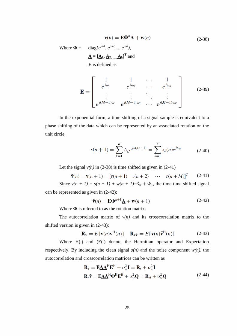
25
(2-38)
Where Φ = diag{ej1
, ej2
, ... ejk
),
A = [A1, A2, ..... Ak]T and
E is defined as
(2-39)
In the exponential form, a time shifting of a signal sample is equivalent to a
phase shifting of the data which can be represented by an associated rotation on the
unit circle.
(2-40)
Let the signal v(n) in (2-38) is time shifted as given in (2-41)
(2-41)
Since v(n + 1) = s(n + 1) + w(n + 1)= , the time time shifted signal
can be represented as given in (2-42):
(2-42)
Where Φ is referred to as the rotation matrix.
The autocorrelation matrix of v(n) and its crosscorrelation matrix to the
shifted version is given in (2-43):
(2-43)
Where H(.) and (E(.) denote the Hermitian operator and Expectation
respectively. By including the clean signal s(n) and the noise component w(n), the
autocorrelation and crosscorrelation matrices can be written as
(2-44)

26
Where
(2-45)
For the signal subspace, the generalized eigenvalue problem can be written as
(2-46)
Where is the eigenvector of . By substituting the expression in
(2-44) into (2-46) the following relation is obtained :
(2-47)
The expression in (2-47) can also be written as
(2-48)
The decomposition process is performed by estimating the frequencies of
sinusoid from
where
Once are obtained, the amplitudes and powers of the harmonics can be
estimated in the same way as used in MUSIC (Section 2.5.6).
Similar to other parametric methods such as Prony analysis and MUSIC
algorithm, the total number of components of the signal to be decomposed by the
ESPRIT algorithm needs to be determined prior to the analysis. Otherwise,
inaccurate result will be obtained from the decomposition process.
2.5.8. Hilbert Huang Transform (HHT)
A recent adaptive method to decompose signals is the Hilbert Huang method
(HHT), which is well suited for analysing stationary and non-stationary signals and
thus is well suited method for PQ waveform decomposition. The Hilbert Huang
Transform consists of two distinct processes. First, the Empirical Mode
Decomposition (EMD) process is applied to decompose the signal being analysed to
obtain the signal components represented in the Intrinsic Mode Functions (IMFs).

27
Second, the Hilbert Transform is performed to each IMF to obtain the instantaneous
frequencies, amplitudes and phases [5].
The main advantage of the HHT technique over other PQ decomposition
methods is the high time resolution. The intuitive visual information of the
frequency, amplitude and phase of the signal components is also a valuable result of
analysis using HHT method [38]. This method will be discussed in details in the next
chapter.
2.6. Chapter summary
This chapter has defined the PQ problems, and discussed the classification of a
variety of PQ disturbances and their effects to the equipment. To help identify PQ
problems, PQ meters are required. The analysis of the data collected by the
instruments is needed to decompose the signal for the PQ disturbance identification.
Several methods to decompose non-stationary PQ waveforms have been described.
In summary, the FFT is limited to stationary signals, STFT can be used for non-
stationary signal analysis but it has a fixed resolution which depends on the chosen
window size. The wavelet transform has better resolution than STFT, however it is
not adaptive. The parametric methods such as Prony, MUSIC and ESPRIT algorithm
require to know or assume the number of sinusoids in the signal being analyzed prior
to the decomposition process, and hence these methods cannot be used to decompose
unknown signals. The HHT technique is well suited for analysing stationary and non-
stationary signals and requires no initial assumption of the signal and therefore it is
adaptive to any unknown signals. The method is most suitable for decomposing non-
stationary signals often found in PQ waveforms measured by associated meters. For
this reason, this method has been chosen for use in this research and will be
discussed in details in the next chapter.

28
CHAPTER 3 THE HILBERT HUANG TRANSFORM
(HHT)
3.1 Introduction
This chapter describes the use of HHT in this research to decompose stationary
and non-stationary signals in considerably high time resolution. A brief description
of why the method is needed and the operation of the method are presented. The
advantages and disadvantages of HHT when applied to decompose non-stationary,
noisy and close frequencies PQ signals are discussed.
3.2 Why HHT?
Data analysis is an important part to extract the information from PQ signals
measured by the associated meters. While the data might not be perfect, they
represent the reality at hand. The main purposes of data analysis are to determine the
parameters required to build a model and to confirm that a phenomenon is precisely
represented by a built model [2].
Despite this, physical measurement data or numerical modelling data has a
high probability of having the following issues, either the total range of data is not
long enough, it is non-stationary, or represents nonlinear processes. Each problem
can represent itself independent of other problems or in conjunction, but it is
important to note that the first two listed above can be related to each other, as data
that appears to be non-stationary can be a result of data that is shorter than the
longest time scale of a stationary process. In regards to these problems, there is little
we can do in terms of analysis [2].
Historically, the Fourier spectral type of data analysis gave us with a standard
data analysis method to examine global energy-frequency distributions. The usage of
the terminology 'spectrum' has come to be associated with the Fourier transformation
method. Fourier analysis has been the primary method for data analysis since the first
time it was introduced, and continues to be widely used for the analysis due to its
intrinsic ability and simplicity.
Although it has been demonstrated by some researchers that Fourier
transformation is valid in a range of general conditions, (for example, see Titchmarsh
[39]), there are some key restrictions of this method. Firstly the system must be
linear, and the data be precisely periodic or stationary. If this is not the case,

29
erroneous result can be obtained [2]. However, most of PQ signals are non-
stationary, with data sets usually of finite duration and from often systems which are
by design non-linear. Therefore, there is a limitation of applying Fourier Transform
for PQ signal analysis. For example, according to International Electrotechnical
Commission (IEC) standard, signals whose amplitudes vary with time cannot be
described correctly by their harmonic components (obtained from the FFT spectrum)
only. Therefore, a grouping method is suggested to resolve the issue of describing
such signal [18].
HHT has been devised as a data analysis method with its basis on the
Empirical Mode Decomposition (EMD) method, which extracts the components of
the signal represented as a set of Intrinsic Mode Functions (IMFs) without the need
of any assumption prior to the analysis. Basically, the decomposition identifies
directly the instantaneous energy associated with various time scales to extract the
IMFs which have well-behaved Hilbert transforms. The instantaneous frequency can
then be calculated from the IMFs using the Hilbert Transform to localize any event
by time and by frequency [2].
3.3 The Basic of HHT
As described in Section 3.2, the Hilbert Huang Transform consists of two
distinct processes. First, the Empirical Mode Decomposition (EMD) process is
applied to decompose the signal being analysed to obtain the signal components
represented in the Intrinsic Mode Functions (IMFs). Once the IMFs are obtained, the
Hilbert Transform process is then applied to each IMF to obtain the instantaneous
frequencies amplitudes and phases [5]. In this research, the MATLAB code available
online is used to perform the analysis using the standard HHT method [40].
3.3.1 Empirical Mode Decomposition (EMD)
EMD is designed to analyse oscillatory signals, but is not limited to describing
these signals in terms of a sum of sinusoids as the Fourier method does. Changes in
frequency or amplitude within an oscillatory period can be detected when EMD is
paired with Hilbert Transform in a process called the Hilbert-Huang Transform
(HHT). EMD is also not limited to stationary signals in that it adapts to changes in
the signal. A number of studies have used EMD on physical problems including
climate data, ocean waves, testing for structural damage, and image analysis. It is

30
reported that the EMD has extracted physically meaningful components in many of
these applications [41].
Each IMF resulting from EMD process has to satisfy the following conditions
[5].
(a) There is exactly one zero between any two consecutive local extremas.
(b) The “local mean” has to be zero
A signal that satisfies the IMF conditions allows for instantaneous frequency
and amplitude to be clearly defined [6].
The IMFs are extracted through a sifting process in the EMD algorithm. Sifting
is used to subtract away large-scale features of the signal consecutively until only
fine-scale features are left. Once the sifting process is done, a signal S(t) is separated
into the fine-scale oscillation d(t) which will become the first IMF and the residual
r(t) which may replace the original signal to go through the next sifting process [6].
The process will be repeated in iterative fashion as long as the residue / signal to be
processed have at least 3 extremas. When the residue / signal has less than 3
extremas indicating that the scale has become very large, the EMD process is then
terminated. The last waveform remaining from the process is not an IMF but the
trend of the original signal.
In the sifting process, it is necessary to have a local mean of the signal, which
can be obtained by identifying the local maxima and minima of the signal. The
maximum and minimum envelopes are then created using natural cubic splines
connecting the respective local extrema. The mean of the two envelopes is used for
the approximation of the local mean. [6]
A flowchart describing the algorithm of the EMD process is shown in Figure
3.3.1.1.
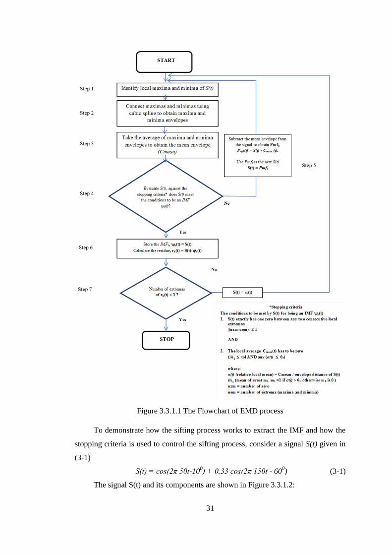
31
Figure 3.3.1.1 The Flowchart of EMD process
To demonstrate how the sifting process works to extract the IMF and how the
stopping criteria is used to control the sifting process, consider a signal S(t) given in
(3-1)
S(t) = cos(2π 50t-100) + 0.33 cos(2π 150t - 60
0) (3-1)
The signal S(t) and its components are shown in Figure 3.3.1.2:

32
Figure 3.3.1.2: The components of signal S(t), (a) 50Hz component
(b) 150 Hz component (c) The signal S(t)
The EMD process is then performed according to the flowchart shown in
Figure 3.3.1.1 as follows :
Step 1: Identify the local maxima and minima of the signal S(t). Figure 3.3.1.3
shows the signal with identified maxima and minima at iteration 0.
Figure 3.3.1.3 The signal with identified maxima and minima
Step 2. By using cubic spline interpolation, connect all of the maxima to obtain
the maximum envelope Cmax(t) and connect all of the minima to obtain
the minimum envelope Cmin(t). The signal with identified maximum and
minimum envelopes is shown in Figure 3.3.1.4.
a)
b)
c)

33
Figure 3.3.1.4. The signal with maximum and minimum envelopes
Step 3. Calculate the mean of the two envelopes as given by (3-2). The mean
envelope is shown in Figure 3.3.1.5.
Cmean(t) = (Cmax(t) + Cmin(t))/2 (3-2)
Figure 3.3.1.5 The signal with identified mean envelope
Step 4. Test whether S(t) qualifies against the requirements to be an IMF by
checking its waveform. The first condition to be an IMF is that there is
exactly one zero between any two consecutive local extrema or when the
difference between the number of zero and the extrema is less or equal to
1. The waveform of S(t) in Figure 3.3.1.5 indicates that a zero always
exists between each two consecutive local extrema which satisfies the
first condition to be an IMF.
The Cmean(t) waveform of S(t) shown in Figure 3.3.1.5 is then evaluated
against the stopping criteria shown at the bottom part of the flowchart in
Figure 3.3.1.1. Cmean(t) waveform shown in Figure 3.3.1.5 indicates that
its amplitude is still large at this stage (iteration 0). Cmean(t) is then
evaluated to identify how close it is to zero (which is the second
condition to be an IMF). The evaluation is performed by using 3
thresholds (θ1, θ2 and tol) as proposed by Rilling [5]. Threshold θ1 is
designed to guarantee globally small fluctuations of Cmean(t) while
threshold θ2 is used to take into account locally large excursions of

34
Cmean(t) [4]. In this example, the default stopping criteria (θ1 = 0.05,
θ2=0.5 and tol = 0.05) is used [5].
Some variables related to the thresholds which are referred to as
envelope distance a(t) and normalized local mean σ(t) need to be
calculated first as given by (3-3) and (3-4) :
The envelope distance of S(t) denoted by a(t) is given by
a(t) = (Cmax(t) − Cmin(t))/2 (3-3)
Figure 3.3.1.6 shows the waveform of a(t) superimposed on Figure
3.3.1.5.
Figure 3.3.1.6 The waveform of a(t) superimposed on Figure 3.3.1.5
A relative local mean σ(t) is given by:
σ(t) = |Cmean(t)|/a(t) (3-4)
Figure 3.3.1.7 shows the waveform of σ(t) superimposed on Figure
3.3.1.6.
Figure 3.3.1.7 The waveform of σ(t) superimposed on Figure 3.3.1.6
Figure 3.3.1.7 shows Cmean(t), a(t) and σ(t) which will be used to evaluate
the local mean. To guarantee a globally small fluctuation, σ(t) is
compared to θ1 (specified as 0.05), whenever σ(t) > θ1, a variable denoted
by m1 is set to 1, otherwise m1 is 0. A mean value of of m1 denoted by

35
is then compared to a tolerance „tol‟ (specified as 0.05), and if
exceeds tol, this indicates that the resulting Cmean(t) does not meet the
requirement of globally minimum small fluctuation. Only when is
below „tol‟ then a globally small fluctuation is guaranteed. The criterion
that takes into account locally large excursions is obtained by considering
if there is any event where the value of σ(t) is greater than a threshold θ2
(specified as 0.5).
The sifting process is terminated once the difference between the number
of zero and the extrema is less or equal to 1 AND when is less than
tol AND there is no point of σ(t) greater than θ2. The complete stopping
criteria is shown in the relation given by (3-5).
Stop = |(nzm-nem)| 1 AND ( tol AND any (σ(t) θ2)) (3-5)
Figure 3.3.1.8 shows m1 superimposed on Figure 3.3.1.7.
Figure 3.3.1.8 The waveform of m1 superimposed on Figure 3.3.1.7.
Figure 3.3.1.8 shows equals 0.992 which means that the globally
minimum small fluctuation is not met, and therefore the next iterations
are required. From Figure 3.3.1.8, it is obvious that most of the value of
σ(t) are greater than 0.5 and therefore the locally large excursions are
identified which means that S(t) does not satisfy the second condition to
be an IMF.
Step 5. The original signal S(t) is then subtracted by Cmean(t) to obtain Pmfk which
is then considered as the new S(t) to be processed further through step 1
to step 4. Figure 3.3.1.9 shows the obtained Pmfk or the new S(t) with the
identified local mean.

36
Figure 3.3.1.9 The new S(t) with the local mean
Figure 3.3.1.9 shows the new S(t) and the resulting Cmean(t). As
previously, S(t) has to be checked whether it is an IMF or not. Since a
zero exists between each two consecutive local extremas, the first
condition to be an IMF is satisfied by S(t).
To check whether S(t) meets the the second condition to be an IMF, the
closeness of Cmean(t) to zero is then evaluated. First, a(t) and σ(t) are
calculated and the default value of the thresholds are used to do the
evaluation, as shown in Figure 3.3.1.10.
Figure 3.3.1.10 The evaluation of Cmean(t)
Figure 3.3.1.10 shows that σ(t) is now smaller than threshold θ2 (0.5)
which means that there is no more locally large excursion exist in
Cmean(t). The mean value of m1 is now smaller and equal to 0.613.
However, it is still greater than tol (0.05) and therefore a globally small
fluctuation is not met. Since S(t) does not satisfy the second condition to
be an IMF, more iterations are needed to obtain the IMF.
S(t) is again subtracted by Cmean(t) to obtain Pmfk which is then considered
as the new S(t) to be processed further through step 1 to step 4.

37
Figure 3.3.1.11 shows the obtained Pmfk or the new S(t) with the
identified local mean.
Figure 3.3.1.11 The new S(t) with the local mean
Figure 3.3.1.11 shows the new S(t) with a less fluctuating Cmean(t). As
previously, S(t) has to be checked whether it is an IMF or not. Since a
zero exists between each two consecutive local extremas, the first
condition to be an IMF is satisfied by S(t).
To check whether S(t) meets the second condition to be an IMF, the
closeness of Cmean(t) to zero is evaluated. First, a(t) and σ(t) are
calculated and the default value of the thresholds are used to do the
evaluation, as shown in Figure 3.3.1.12.
Figure 3.3.1.12 The evaluation of Cmean(t)
Figure 3.3.1.12 shows that σ(t) is smaller than threshold θ2(0.5) which
means that there is no more locally large excursion exist in Cmean(t). The
value of is now below 0.05 which means that a globally small
fluctuation is met. At this stage, the second condition to be an IMF is
satisfied by S(t), therefore, no more iteration is required.
Step 6 Store S(t) as an IMF and calculate the residue by subtracting the IMF
from the original signal. Figure 3.3.1.13 shows the residue.

38
Figure 3.3.1.13. The first residue of the signal S(t)
Step 7: Test whether the number of local maxima or minima is less than three, if
so terminate the EMD process, otherwise repeat steps 1 - 7 on the residue
rk(t).
Since the number of local maxima and minima of the residue is more
than three, as shown in Figure 3.3.1.13, the residue will then be
considered as the new signal S(t) to be processed through step 1 to step 4.
Figure 3.3.1.14 shows the new S(t) with the identified local Cmean(t).
Figure 3.3.1.14. The new S(t) with the local mean
Figure 3.3.1.14 shows the new S(t) and the resulting Cmean(t) waveform
which indicates that its amplitude is very close to zero at this stage
(iteration 0). The stopping criteria is then used to check the waveform
against the second condition to be an IMF as shown in Figure 3.3.1.15.

39
Figure 3.3.1.15 The evaluation of Cmean(t)
Figure 3.3.1.15 shows that σ(t) is completely smaller than threshold
θ2(0.5) which means that there is no locally large excursion exist in
Cmean(t). Further, Cmean(t) is now below θ1 (0.05) all the time indicated by
continuous zero value of m1. Hence, is now 0 which means that a
globally small fluctuation is met. To this stage, the second condition to
be an IMF is satisfied by S(t), therefore, no more iteration is needed. S(t)
is considered as the next IMF, which is then stored as IMF2.
The second residue rk(t) (k=2) is then calculated by subtracting the IMF2
from S(t). Figure 3.3.1.16 shows the second residue of the process.
Figure 3.3.1.16. The second residue of the process
Figure 3.3.1.16 shows that the second residue does not have sufficient
extrema number according to step 7 to continue the EMD process.
Therefore, the process is terminated. The final result of the
decomposition is shown in Figure 3.3.1.17.

40
Figure 3.3.1.17: The Final result of Empirical Mode Decomposition process on S(t),
(a) The signal S(t), (b) IMF1 (150Hz), (c) IMF2 (50Hz)
Figure 3.3.1.17 demonstrates how the EMD process has succesfully
decomposed the original signal S(t) into its components represented in the IMFs. The
IMFs in Figure 3.3.1.17 (b)-(c) show very similar waveforms to the original
components shown in Figure 3.3.1.2(a)-(b). However, there are small differences at
both ends of the IMFs which is attributed to the end effect problem of the IMFs. End
effect phenomenon is caused by the limitation of cubic spline interpolation to
estimate the maxima and minima envelopes due to insufficient number of extrema
points to be interpolated at both ends of the waveform being analyzed.
3.3.2 Hilbert Transform (HT)
The Hilbert Transform (HT) [6], [42] of x(t) is defined as:
(3-6)
where: P is the Cauchy Principal Value integral
The Hilbert Transform of a real signal xr is an analytic signal x=xr + i*xi where
xr is the original data and the imaginary part i*xi is a version of xr shifted by 900. The
Hilbert transformed signal x has the same amplitude and frequency as the original
data xr with the phase angle depends on the phase angle of xr. [43].
The analytic signal obtained from The Hilbert transform can be used to
determine the instantaneous amplitude, frequency and phase of the original data. For
d
t
xPtxH
)(1)(
a)
b)
c)

41
a pure sinusoid, the instantaneous amplitude, frequency and phase are constant.
However, for the IMF which usually has the end effect issue, the instantaneous
parameters are fluctuating as will be demonstrated in the following paragraphs.
The analytic signal z(t) of a signal x(t) is defined as:
z(t) = x(t) + H[x(t)] = x + jy = a(t) e j(t)
(3-7)
For a pure cosine signal x(t) = A cos(ωt+), the analytic signal contains its sine
version :
z(t) = A cos(ωt+) + j A sin(ωt+) = A e j(ωt+)
(3-8)
For example, a pure cosine signal is given by (3-9) :
S(t) = cos(ωt - 100) (3-9)
where f =50 Hz and ω = 2πf.
The Hilbert Transform of S(t) is shown in Figure 3.3.2.1. The instantaneous
amplitude of S(t) can be calculated as follows [6], [42] :
(3-10)
By applying (3-10) to S(t), the instantaneous amplitude is obtained and shown
in Figure 3.3.2.2, which is a constant value of 1.0.
Figure 3.3.2.1 The Hilbert Transform of S(t).
22)( yxta

42
Figure 3.3.2.2 The instantaneous amplitude of S(t).
The Hilbert Transform is then applied to IMF2 of the signal S(t) shown in Figure
3.3.1.17(c) obtained from the of EMD process to calculate the analytic signal z(t) of
the IMF shown in Figure 3.3.2.3.
Figure 3.3.2.3 The analytic signal z(t) of IMF2 obtained by the Hilbert Transform .
By using the relation in (3-10), the instantaneous amplitude of IMF2 can be
determined as shown in Figure 3.3.2.4. The calculated instantaneous amplitude in
Figure 3.3.2.4 shows that the end effect due to the sifting process can affect the
Hilbert transform of the IMF, and therefore the instantaneous amplitude is not
constant all the time. To find the actual amplitude, the impact of the end effect
should be avoided by taking the mean of the instantaneous amplitude from 10% -

43
90% of the data which result in the estimated amplitude 1.01p.u. The mean value of
the instantaneous amplitude is shown by the red line in Figure 3.3.2.4.
Figure 3.3.2.4: The instantaneous amplitude of IMF2.
The instantaneous phase angle (t) can be calculated from the instantaneous x
and y values of the signal as given in (3-11)
(3-11)
Applying Equation (3-11) to the pure sinusoid signal S(t) will result in a saw
tooth instantaneous phase signal shown in Figure 3.3.2.5, since (t) = (ωt - 100):
Figure 3.3.2.5 The instantaneous phase angle of S(t).
To obtain the actual instantaneous phase values, the result in Figure 3.3.2.5
needs to be subtracted by ωt (this can be done since the frequency f is known and
equals to 50 Hz), as shown in Figure 3.3.2.6, showing that the instantaneous phase is
constant and equals to -100
as expected.
x
yt arctan)(

44
Figure 3.3.2.6 The instantaneous phase angle of S(t) after the subtraction.
However, for most general cases, the frequency ω is not known and hence it
needs to be estimated by using the relation given in (3-12).
(3-12)
and
f(t) =ω(t)/(2π)
Once the estimated ω is obtained, it can be subtracted from the instantaneous
phase angle (t) to obtain the initial phase angle.
The formula given in (3-12) provides the instantaneous frequency of S(t)
which is constant at 50 Hz, as expected. The instantaneous frequency is shown in
Figure 3.3.2.7.
Figure 3.3.2.7 The instantaneous Frequency of S(t).
dt
dt
)(

45
Now the instantaneous frequency of IMF2 can be calculated using the relation
given in (3-12), and the estimated instantaneous frequency is shown in Figure
3.3.2.8. As previously, the end effect due to the EMD sifting process also appears in
the Hilbert Transform result.
To improve the result of instantaneous frequency estimation, a Matlab function
instfreq.m available online [40] is used. For an analytic signal x at time instant(s) t,
instfreq.m performs the instantaneous frequency estimation of x by using trapezoidal
integration rule. The estimated instantaneous frequency using instfreq.m is also
shown in Figure 3.3.2.8 which demonstrates an improvement at both ends of the
instantaneous frequency waveform.
To find the actual frequency, the impact of the end effect should be avoided by
taking the mean of the instantaneous frequency from 10% - 90% of the data which
result in the estimated actual frequency 50.04 Hz.
Figure 3.3.2.8: The instantaneous Frequency of IMF2.
The initial phase angle can now be calculated for IMF2 by calculating the
Instantaneous phase using Equation (3-11) and subtract it by ω as previously and the
result is shown in Figure 3.3.2.9. The mean of the result from 10% - 90% of data is
also used to determine the phase angle of the signal, which is equal to -100.

46
Figure 3.3.2.9: The instantaneous phase angle of IMF2.
Figures 3.3.2.4, 3.3.2.8 and 3.3.2.9 show that the end effect issue causes
inaccuracy in the calculated instantaneous amplitude, frequency and phase since the
IMF is not a pure sinusoid with a constant amplitude. To avoid this end effect issue,
the mean of the instantaneous values from 10% - 90% of the data is used to calculate
the estimated value of the amplitude, frequency and phase. Such technique to avoid
the end effect issue is used in the whole thesis to obtain the more accurate value of
amplitude, frequency and phase to correct the original result from applying Hilbert
Transform to each IMF.
Applying the Hilbert transform directly to a multi-component signal provides
values of a(t) and f(t) which are unusable for describing the signal. For example if
the Hilbert Transform is applied directly to the signal given in (3-1) then the result is
shown in Figure 3.3.2.10.
Figure 3.3.2.10. The Hilbert Transform applied on a multicomponent signal.
(a) The multi-component signal (b) Instantaneous frequency (c) Instantaneous
Amplitude
a)
b)
c)

47
Figure 3.3.2.10 shows that applying HT on a multi-component signal produces
fluctuating instantaneous frequency and instantaneous amplitude which is caused by
the mixed frequency (multi-components) contained in the signal.
For this reason, the Empirical Mode Decomposition is needed to first
decompose the signal into IMFs each of which contains single component of the
signal, which can then be processed by the Hilbert Transform to obtain meaningful
instantaneous attributes of the IMFs.
3.4 Applying HHT to Stationary Signals
To demonstrate the effectiveness of HHT to decompose stationary signals,
several PQ signals such as harmonics and flicker are analysed.
3.4.1 PQ waveform with harmonics
Consider a signal that contains 3rd
and 11th
harmonic
S(t) = sin(2π 50t + 300) + 0.33 sin(2π 150t + 30
0) +
0.09 sin(2π 550t + 300) (3-13)
The results from applying the EMD process to the signal given by (3-13) are
shown in Figure 3.23. Figure 3.23 shows that the EMD process has decomposed the
signal correctly to three IMFs, each of which represents the component of the signal.
Figure 3.4.1.1 The EMD process of S(t)
Applying the Hilbert Transform to each of the IMFs produces the
instantaneous amplitude, frequency and phase of each component as shown in Figure
3.4.1.2.

48
Figure 3.4.1.2 The instantaneous frequency, amplitude and phase of the detected
IMFs of S(t). (a) IMF1, (b) IMF2, (c) IMF3
Since the IMFs generated by the EMD process suffer the end effect problem,
the mean value of 10% - 90% length of the instantaneous variable is used to obtain
the actual amplitude, frequency and initial phase shown in Table 3.1.
Table 3.1
The result of The Hilbert Transform of the IMFs of S(t)
True
Freq
(Hz)
Freq
calc. by
HHT
(Hz)
True
Amp
(p.u)
Amp
calc. by
HHT
(Hz)
True
Phase
(deg)
Phase
calc. by
HHT
(deg)
550 550 0.09 0.09 30 30.1
150 150 0.33 0.33 30 31.14
50 50 1 1 30 30.2
Table 3.1 shows that the results obtained using HHT are quite accurate in
determining the amplitude, frequency and phase of the components of the analysed
signal.
(a) (b)
(c)
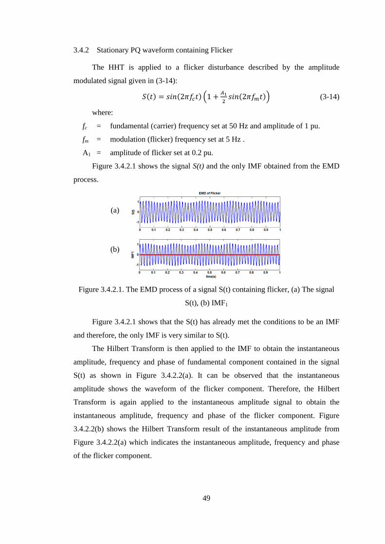
49
3.4.2 Stationary PQ waveform containing Flicker
The HHT is applied to a flicker disturbance described by the amplitude
modulated signal given in (3-14):
( ) ( ) (
( )) (3-14)
where:
fc = fundamental (carrier) frequency set at 50 Hz and amplitude of 1 pu.
fm = modulation (flicker) frequency set at 5 Hz .
A1 = amplitude of flicker set at 0.2 pu.
Figure 3.4.2.1 shows the signal S(t) and the only IMF obtained from the EMD
process.
Figure 3.4.2.1. The EMD process of a signal S(t) containing flicker, (a) The signal
S(t), (b) IMF1
Figure 3.4.2.1 shows that the S(t) has already met the conditions to be an IMF
and therefore, the only IMF is very similar to S(t).
The Hilbert Transform is then applied to the IMF to obtain the instantaneous
amplitude, frequency and phase of fundamental component contained in the signal
S(t) as shown in Figure 3.4.2.2(a). It can be observed that the instantaneous
amplitude shows the waveform of the flicker component. Therefore, the Hilbert
Transform is again applied to the instantaneous amplitude signal to obtain the
instantaneous amplitude, frequency and phase of the flicker component. Figure
3.4.2.2(b) shows the Hilbert Transform result of the instantaneous amplitude from
Figure 3.4.2.2(a) which indicates the instantaneous amplitude, frequency and phase
of the flicker component.
(a)
(b)

50
Figure 3.4.2.2: The Hilbert Transform to obtain instantaneous frequency, amplitude
and phase angle of (a) The signal contains Flicker (b) The flicker signal
To obtain more accurate result of the Hilbert Transform, the mean value of
10% - 90% length of the instantaneous amplitude, frequency and phase of the IMFs
is again used. The result from the Hilbert Transform is shown in Table 3.2.
Table 3.2
The Hilbert Transform of IMFs of Flicker signal
fc (carrier component)
True
Freq
(Hz)
Freq
calc. by
HHT
(Hz)
True
Amp
(p.u)
Amp
calc. by
HHT
(Hz)
True
Phase
(deg)
Phase
calc. by
HHT
(deg)
50 50 1 1 0 0
fm (modulation / flicker component)
True
Freq
(Hz)
Freq
calc. by
HHT
(Hz)
True
Amp
(p.u)
Amp
calc. by
HHT
(Hz)
True
Phase
(deg)
Phase
calc. by
HHT
(deg)
5 5 0.1 0.1 0 0
Table 3.2 shows that the HHT method has succesfully decomposed the signal
contains flicker.
3.5 Applying HHT to Non-Stationary Signals
To demonstrate the effectiveness of HHT to decompose non-stationary signals,
several PQ signals such as sag, swell and transient are analysed in this section.
a) b)

51
3.5.1 Non-stationary PQ waveform with harmonics and sag
The HHT is applied to a non-stationary PQ signal with harmonics and sag as
follows :
sttt
sttt
sttt
tS
ccc
bbb
aaa
A
3.02.0),2502sin(2.0)502sin(
2.01.0),2502sin(16.0)502sin(8.0
1.00),2502sin(2.0)502sin(
)(
(3-15)
The resulting IMFs obtained from the EMD process from the signal given in
(3-15) are shown in Figure 3.5.1.1 and the associated instantaneous amplitude,
frequency and phase obtained from the Hilbert Transform of the IMFs are shown in
Figure 3.5.1.2.
Figure 3.5.1.1 The EMD process on a signal SA(t) with harmonic and sag.
(a) The Signal SA(t) (b) IMF1 (c) IMF2
Figure 3.5.1.2. The result from Hilbert Transform of SA(t): (a) Instantaneous
Amplitude, (b) Instantaneous frequency (c) Instantaneous Phase
a)
b)
a)
b)
c)
c)

52
It is observed in Figure 3.5.1.2, that the HHT method can obtain automatically
the instantaneous amplitude, frequency and phase of both signals in the non-
stationary signal. However, inaccuracies occur in the calculated instantaneous
amplitude, frequency and phase around the area of transitions / discontinuities
leading to overshoot and ambiguity.
3.5.2 Windowing Technique [38]
The inaccuracy issue around the area of transitions can be mitigated by using a
windowing technique [38] which applies the HHT over a sliding window of the
signal S(t) to identify the instant of changes (boundaries) of the non-stationary signal.
Once the boundaries are identified, the HHT can then be applied to each segment
(the area between two boundaries) which contains stationary part of the original
signal. For example, a window size of 0.02 sec is chosen and therefore the HHT is
applied to S(t) from 0.0 to 0.02 sec, 0.02 - 0.04 sec and so on. When there is a change
in frequency or amplitude of the first IMF of a particular window, the first point of
the window is marked as a boundary of a segment of the signal. For the signal with
harmonic and sag, the instant of changes are found at 0.1 sec and 0.2 sec. When the
boundaries of all the segments are identified, the HHT is applied to the individual
segment to obtain more accurate result.
The result of the windowing technique for signal S(t) is shown in Figure
3.5.2.1 and Table 3.3 which shows that an accurate instantaneous amplitudes,
frequencies and phases are found with clear points of change during transition and
very accurate results are obtained for each component of each segment from the non-
stationary signal. For a more accurate method to determine the instant of change, a
novel use of Symbolic Aggregate Approximation will be introduced and described in
Chapter 5.

53
Figure 3.5.2.1. The result from windowing technique on SA(t): (a) Instantaneous
Amplitude, (b) Instantaneous frequency (c) Instantaneous Phase
Table 3.3
The result from windowing technique and HHT of SA(t)
0s t < 0.1s 0.1 s t < 0.2 s 0.2 s t 0.3 s
Amp
(p.u)
Freq
(Hz)
Phase
(deg)
Amp
(V)
Freq
(Hz)
Phase
(deg)
Amp
(p.u)
Freq
(Hz)
Phase
(deg)
0.2 250 - 0.02 0.16 250 0 0.2 250 0.02
1.0 50 0.1 0.8 50 0 1.0 50 -0.1
3.5.3 Non-stationary PQ waveform with harmonics and swell
The HHT is applied to a non-stationary signal SB(t) with harmonics and swell
as follows :
sttt
sttt
sttt
tS
ccc
bbb
aaa
B
3.02.0),2502sin(2.0)502sin(
2.01.0),2502sin(24.0)502sin(2.1
1.00),2502sin(2.0)502sin(
)(
(3-16)
The resulting IMFs obtained from the EMD process of the signal given in (3-
16) are shown in Figure 3.5.3.1 and the associated instantaneous amplitude,
frequency and phase are shown in Figure 3.5.3.2.
a)
b)
c)
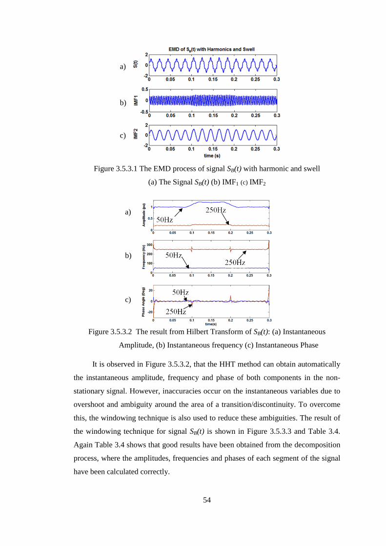
54
Figure 3.5.3.1 The EMD process of signal SB(t) with harmonic and swell
(a) The Signal SB(t) (b) IMF1 (c) IMF2
Figure 3.5.3.2 The result from Hilbert Transform of SB(t): (a) Instantaneous
Amplitude, (b) Instantaneous frequency (c) Instantaneous Phase
It is observed in Figure 3.5.3.2, that the HHT method can obtain automatically
the instantaneous amplitude, frequency and phase of both components in the non-
stationary signal. However, inaccuracies occur on the instantaneous variables due to
overshoot and ambiguity around the area of a transition/discontinuity. To overcome
this, the windowing technique is also used to reduce these ambiguities. The result of
the windowing technique for signal SB(t) is shown in Figure 3.5.3.3 and Table 3.4.
Again Table 3.4 shows that good results have been obtained from the decomposition
process, where the amplitudes, frequencies and phases of each segment of the signal
have been calculated correctly.
a)
b)
c)
a)
b)
c)

55
Figure 3.5.3.3: The result from windowing technique of signal SB(t):
(a) Instantaneous Amplitude, (b) Instantaneous frequency (c) Instantaneous Phase
Table 3.4.
Result from windowing technique and HHT of SB(t)
0s t < 0.1s 0.1 s t < 0.2 s 0.2 s t 0.3 s
Amp
(p.u)
Freq
(Hz)
Phase
(deg)
Amp
(p.u)
Freq
(Hz)
Phase
(deg)
Amp
(p.u)
Freq
(Hz)
Phase
(deg)
0.2 250 - 0.02 0.239 250 0 0.2 250 0.02
1.0 50 0.1 1.2 50 0 1.0 50 -0.1
3.5.4 Non-stationary PQ waveform with transient
The HHT is applied to a non-stationary signal with harmonics and transient
SC(t) as follows (3-17):
sttt
stettt
sttt
tS
ccc
b
t
bbb
aaa
C
b
3.018.0),2502sin(2.0)502sin(
18.01.0,)5002sin()2502sin(2.0)502sin(
1.00),2502sin(2.0)502sin(
)()1.030(
(3-17)
The transient signal is shown in Figure 3.5.4.1. The resulting IMFs obtained
from the EMD process from the signal in (3-17) are given in Figure 3.5.4.2 and the
associated instantaneous amplitude, frequency and phase obtained from the Hilbert
Transform are given in Figure 3.5.4.3.
a)
b)
c)

56
Figure 3.5.4.1 The signal SC(t) contains transient
Figure 3.5.4.2 The resulting IMFs of a transient signal SC(t)
Figure 3.5.4.3 The Hilbert Transform of IMFs of SC(t): (a) IMF1, (b) IMF2, (c) IMF3
It is observed in Figure 3.5.4.3, that the HHT method can obtain automatically
the instantaneous amplitude, frequency and and phase of signal components in the
non-stationary signal SC(t). However, inaccuracies occur in the instantaneous
variables due to overshoot and ambiguity around the area of a
transition/discontinuity. To overcome this, the windowing technique is then used to
(a) (b) (c)

57
reduce these ambiguities. The windowing technique is applied to detect if any change
in frequency occurs in the first IMF of a particular window, then the first point of the
window is marked as a boundary for a segment.
The boundaries are identified correctly at t1 = 0.1sec and t2 = 0.18sec. Once the
segments are identified, the HHT is then applied to the signal over the identified
segments to obtain the instantaneous frequency, amplitude and phase. The result of
the windowing technique for signal SC(t) is shown in Figure 3.5.4.4 and Table 3.5.
Figure 3.5.4.4 The result from windowing technique of signal SC(t): (a) IMF1,
(b) IMF2, (c) IMF3
Table 3.5
The result from windowing technique and HHT of a transient signal SC(t)
IMF
No Seg 1, 0s t < 0.1 Seg 2, 0.1 s t < 0.18 s Seg 3, 0.18 s t 0.3 s
Amp
(p.u)
Freq
(Hz)
Phase
(deg)
Amp
(p.u)
Freq
(Hz)
Phase
(deg)
Amp
(p.u)
Freq
(Hz)
Phase
(deg)
1 0.2 250 0.2 e(-30t-0.1)
500 0.4 0.2 250 0.15
2 1.0 50 0.0 0.2 250 3.3 1.0 50 0.01
3 0 0 0.0 1.0 50 2.6 0 0 0
Table 3.5 shows the detected amplitudes, frequencies and phases of the IMFs
from the EMD process of signal SC(t). In the EMD process, the highest frequency
component of the signal will be captured by IMF1 and the next highest frequency
component is represented by IMF2 and so on. Therefore, IMF1 captures the highest
frequency component of each segment, 250 Hz at segment 1, 500 Hz at segment 2
and 250 Hz at segment 3. The waveform of IMF1 and the associated instantaneous
amplitude, frequency and phases are shown in Figure 3.5.4.4(a). IMF2 captures the
lower frequency component of each segment, 50 Hz at segment 1, 250 Hz at segment
2 and 50 Hz at segment 3. The waveform of IMF2 and the associated instantaneous
amplitude, frequency and phases are shown in Figure 3.5.4.4(b). IMF3 captures the
(a) (b) (c)

58
lowest frequency component of each segment. Since there is no lower than 50 Hz
frequency in the signal, no frequency, amplitude and phase are detected in segment 1
and 3. The lowest frequency 50 Hz is detected in segment 2. The waveform of IMF3
and the associated instantaneous amplitude, frequency and phases are shown in
Figure 3.5.4.4(c).
As shown in Figure 3.5.4.4(a), the exponential sinusoidal waveform is
captured in second segment of IMF1 after applying HHT to the IMF. The Hilbert
Transform of IMF1 provides the associated instantaneous frequency, amplitude and
phase. The instantaneous amplitude of IMF1 shows a waveform decays exponentially
in segment 2. To identify the waveform, an exponential curve fitting is used to
predict an exponential expression as shown in Table 3.5.
Figure 3.5.4.4 and Table 3.5 demonstrate that the EMD method with
windowing technique can decompose the non-stationary signal with transient SC(t)
accurately.
3.6 Issues in implementing HHT
There are a number of issues faced when implementing HHT. Cautious steps
need to be taken to obtain satisfactory results from the HHT process.
3.6.1 Stopping Criteria
The sifting process used in the EMD algorithm to extract the IMFs from the
signal has to be carried out iteratively until the conditions for being an IMF are
fulfilled. To guarantee that the local mean is very close to zero (which is the second
condition to be an IMF), a stopping criterion using 3 thresholds (θ1, θ2 and tol) has
been designed [5]. Threshold θ1 and tol are designed to guarantee globally small
fluctuations of the IMF while threshold θ2 is used to take into account locally large
excursions of the IMF. The threshold of the stopping criterion needs to be specified
appropriately since too small a threshold may cause over decomposition, and too
large a threshold may cause poor decomposition i.e some of the signal components
remain unidentified.
Based on many simulations, setting the value of stopping criteria smaller than
the default can provide a better decomposition result, however, using too small a
threshold can lead to over-iteration that can cause over-decomposition.

59
As an example of the effect of various stopping criteria to the decomposition
result, consider a signal S(t) as given in (3-18) :
S(t) = sin(2π 50t + 00) + 0.2 sin(2π 250t + 0
0) +
0.14 sin(2π 350t + 00) (3-18)
When the default stopping criteria (θ1 = 0.05, θ2 = 0.5 and tol = 0.05) is
chosen to decompose the signal by using the HHT, the result is shown in Table 3.6
Table 3.6
Result of HHT decomposition of the signal S(t)
Using θ1= 0.05, θ2 = 0.5 and tol = 0.05
True
Freq
(Hz)
Freq Calc
using HHT
(Hz)
True
Amp
(pu)
Amp Calc
using HHT
(pu)
True Phase
(Deg)
Phase Calc
using HHT
(deg)
350 350 0.14 0.18 0 0.03
250 None 0.2 None 30 None
50 50 1.0 1 0 0.003
Table 3.6 shows that the HHT using the default stopping criteria does not
decompose the signal accurately, since the 250 Hz component is not detected.
When a smaller stopping criteria (θ1= 0.0005, θ2 = 0.005 and tol = 0.0005) is
used, the result of the HHT is shown in Table 3.7.
Table 3.7
Result of HHT decomposition of the signal S(t)
using θ1= 0.0005, θ2 = 0.005 and tol = 0.0005
True
Freq
(Hz)
Freq Calc
using HHT
(Hz)
True Amp
(pu)
Amp Calc
using HHT
(pu)
True Phase
(Deg)
Phase Calc
using HHT
(deg)
350 350 0.14 0.14 0 0.03
250 250 0.2 0.18 0 0
50 50 1.0 1 0 0
Table 3.7 shows that if a smaller stopping criteria is chosen, a more accurate
decomposition result is obtained. The 250 Hz component is now detected and the
results of the instantaneous amplitude, frequency and phase are very close to the
specified values.
Further check is then performed by using even smaller stopping criteria (θ1=
5.10-11
, θ2 = 5.10-10
and tol = 5.10-11
) and the maximum number of iteration is set as
5.105. The result of the HHT is shown in Table 3.8.

60
Table 3.8
Result of HHT decomposition of the signal S(t)
using θ1= 5.10-11
, θ2 = 5.10-10
, tol = 5.10-11
and MAXITERATION = 5.105
True
Freq
(Hz)
Freq Calc
using HHT
(Hz)
True Amp
(pu)
Amp Calc
using HHT
(pu)
True Phase
(Deg)
Phase Calc
using HHT
(deg)
350 350 0.14 0.14 0 0.03
250 250 0.2 0.182 0 0
50 50 1.0 0.97 0 2.04
None 45 None 0.092 None 77.53
None 35 None 0.06 None 46.25
Table 3.8 shows that when even smaller stopping criteria is chosen, the
decomposition results are relatively the same with the result obtained by using
greater stopping criteria (Table 3.7). However, some extra signals contain other
frequencies (45 and 35 Hz) with significant amplitudes (0.092 and 0.06 pu) emerge
in the decomposition result. These extra IMFs are not part of the specified
components of the original signal which means that the EMD process does not give
accurate result for this case.
The result in Table 3.8 demonstrates that imposing too small a stopping
criteria will produce over decomposed result which is not desirable. Therefore, the
correct choice of stopping criteria is necessary to obtain accurate results.
The usual practice to select θ1, θ2 and tol used in the research is by initially
selecting the default stopping criteria for the EMD process. When the result is not
accurate, multiply the default stopping criteria by 0.1 to make it smaller. Repeat the
process as necessary. Based on many simulations of PQ signals decomposition in the
research, the smaller stopping criteria such as 0.01 x default (θ1= 0.0005, θ2 = 0.005
and tol = 0.0005) generally produce accurate results to separate the components of
PQ signal containing higher frequency components. More discussions on the effect
of the stopping criterion to the separation of higher frequency components are
presented in Chapter 4.
3.6.2 Close Frequency
The EMD has been found to have difficulty in resolving waveforms containing
components with close frequencies with a ratio of less than two [44]. Such signals
are often encountered in PQ waveforms, for example 9th
, 11th
and 13th
harmonics.

61
When the standard EMD is applied to the signal, IMFs with mixed frequencies may
be obtained.
As an example, consider a signal S(t) as the following :
)306502sin(077.0
)305502sin(091.0)30502sin()(
0
00
t
tttS
(3-19)
Since the signal contains 11th
and 13th
harmonic frequencies that are close
together, the EMD process will produce IMFs that contains mixed frequency, as
shown in Figure 3.6.2.1.
Figure 3.6.2.1. EMD process on a signal that contains close frequency
(a) The signal S(t), (b) IMF1, (c) IMF2,
Figure 3.6.2.1(b) shows IMF1 which looks like a modulated signal composed
from more than one frequency. IMF2 shown in Figure 3.6.2.1(c) looks very similar to
a pure sinusoidal which means it is not mixed with any other frequency.
Generally, mixed frequency IMF (or mode mixing) is not desirable, since it
would produce incorrect results when the IMFs are processed by the Hilbert
Transform as shown in Figure 3.6.2.2 and Table 3.9.
(a)
(b)
(c)

62
.
Figure 3.6.2.2 Hilbert Transform of the IMFs from EMD process on a signal
that contains close frequency (a) IMF1, (b) IMF2,
The IMF1‟s waveform in Figure 3.6.2.2(a) shows fluctuating instantaneous
frequency, amplitude and phase angle plot which indicates that the IMF contains
mixed frequency signal. IMF2‟s waveform in Figure 3.6.2.2(b) shows more stable
instantaneous frequency, amplitude and phase angle values indicating that the IMF is
not mixed. Since one of the IMFs is mixed, applying Hilbert Transform on these
IMFs will produce inaccurate results. Table 3.9 shows the result of HHT on signal
S(t).
Table 3.9
Result of HHT decomposition of the signal S(t)
True
Freq(Hz)
Freq Calc
using HHT
(Hz)
True Amp
(pu)
Amp Calc
using HHT
(pu)
True Phase
(Deg)
Phase Calc
using HHT
(Deg)
650 650 0.0770 0.1022 30 31
550 None 0.0910 None 30 None
50 50 1.0000 1.0220 30 30
Table 3.9 shows that the EMD process has succesfully extracted the 650 Hz
and 50 Hz components, however, the 550 Hz component is not identified by the
EMD algorithm. To overcome the problem with components containing close
frequencies, a novel Iterative Hilbert Huang transform (IHHT) will be proposed in
Chapter 4.
(a) (b)

63
3.6.3 Noise
The EMD has also been found to have mode mixing issues when it is applied
to a signal that contains relatively high level of noise. The noise content of the signal
which is usually of high frequency may mix with a high frequency component of the
signal in the same IMF [8]. To demonstrate the issue, a simulated noisy signal is
created from the formula given by (3-20) :
S(t)= cos(2π 50t) + 0.33cos (2π 150t + 600) + 0.2cos(2π 250t + 50
0) (3-20)
A Gaussian white noise signal with a Signal to Noise Ratio (SNR) = 30 is
added to S(t) to obtain a noisy signal which is then analyzed by the HHT process.
The IMFs obtained from the EMD process of the signal are shown in Figure 3.6.3.1.
The result of the Hilbert Transform applied to the IMFs are shown in Table 3.10.
Figure 3.6.3.1 EMD process of a signal that contains noise, (a) The Signal S(t)
(b) IMF1, (c) IMF2, (d) IMF3, (e) IMF4, (e) IMF5
Figure 3.6.3.1 shows that the EMD process extracts the noise content in IMF1
and IMF2. The high frequency noise is mixed with some portions of 250Hz
component in IMF3 which causes the rest of 250 Hz component to mix with the 150
Hz component in IMF4. This also causes the rest of 150 Hz component is then mixed
with 50 Hz component in IMF5. Table 3.10 shows the results from the Hilbert
Transform of the IMFs.
(a)
(b)
(c)
(d)
(e)
(f)

64
Table 3.10
The Hilbert Transform of the IMFs from EMD process
of signal S(t) in (3-20)
IMF Amp
(p.u)
Freq
(Hz)
Phase
(deg)
1 0.026 3424 -3.42
2 0.015 1786 4.04
3 0.152 335 -3.89
4 0.267 190 -9.39
5 1.019 50 0.18
As shown in Table 3.10, when the Hilbert Transform is applied to process the
mixed IMFs, inaccurate results are obtained, such as the calculated mean value of
instantaneous frequency 335 Hz and 190 Hz, instead of 250 Hz and 150 Hz.
To overcome the problem with components containing high level of noise, a
novel Iterative Ensemble EMD (IEEMD) is proposed in Chapter 6.
3.7 Chapter Summary
This chapter describes the reason of why HHT is used in this research,
followed by the explanation of the basic of HHT which consists of EMD and HT.
The applications of HHT to stationary and non-stationary PQ signals are also
presented showing the effectiveness of HHT to decompose such signals. A simple
windowing technique is proposed to overcome the problem with transitions in non-
stationary signals. In chapter 5, a more advanced method of solving the transition
problems using a Symbolic Aggregated Approximation is described.
Several issues in implementing HHT are also discussed, such as the
determination of the stopping criteria, the mode mixing issues caused by signals
containing close frequency components and signal containing noise. The problem of
mode mixing is the primary difficulty in using HHT for PQ study, since a lot of PQ
signals contain close frequency and noise. Solutions to the mode mixing problems
will be discussed in Chapter 4 and Chapter 6.

65
CHAPTER 4 METHODS TO IMPROVE HHT
4.1. Introduction
This chapter initially describes several techniques from the literature to
improve the HHT method in resolving the mode mixing problem caused by signals
having close frequency components. All these techniques demonstrate the ability to
decompose the close frequency components of the signal. However, they have
disadvantages, in that some assumptions have to be made prior to the analysis and
some requires the use of FFT to obtain the frequency of the components prior to
HHT decomposition. A new method using an iterative process is proposed to
improve the HHT when dealing with signals containing close frequency components,
which does not require the masking signal or FFT to be performed prior to the
analysis. The proposed method referred to as the Iterative HHT is then applied on
various stationary signals with close frequencies to demonstrate its effectiveness.
4.2. Method to improve HHT using Masking Signal
One of the methods that has been proposed to improve the problem of mode
mixing which caused by close frequency components with the ratio of the high
frequency to the low (next highest) frequency being less than 2, is to use the masking
signal [6], [7].
The basic idea of the method is to add an extra signal to the signal being
analysed. Suppose that x(t) is a PQ signal containing two close frequencies fa and fb
(fa>fb) which usually cause the mode mixing issue in the EMD process. By adding an
appropriately chosen masking signal to x(t), the additional signal will prevent the
lower frequency component fb from being mixed with the higher frequency
component fa in an IMF [6].
4.2.1. EMD using Masking Signal [6]
The following algorithm can be used to perform EMD using masking signal :
1. Apply EMD to the original signal x(t) to obtain its IMFs.
2. Estimate the frequency the masking signal, q(t). The frequency can
be calculated from instantaneous frequency f1(t), its mean value and
instantaneous amplitude a1(t) obtained from the Hilbert Transform of the
first IMF. Relation (4-1) provides the estimated masking signal frequency ,
66
obtained from the instantaneous value of f1(i) and the associated a1(i). The
instantaneous value f1(i) and a1(i) are used in (4-1) if any data point of f1(i)
is greater than :
∑ ( )
( )
∑ ( ) ( )
(4-1)
3. The masking signal ( ) is then constructed as
( ) ( ) (4-2)
Based on his experimental results, Rilling recommends to set the value of
m1 equals to 1.6 to multiply the mean value of the instantaneous amplitude,
[6]. Further, the simulations of PQ signal analysis carried out in the
research suggest to use the masking signal with a higher frequency which
produce better result to avoid mode mixing. Therefore, to decompose PQ
signals, is multiplied by m2 which is chosen as 1.2.
4. Perform EMD on x+(t)= x(t) + q(t) to obtain the IMFs z+(t). Similarly
perform EMD on x−(t)= x(t) − q(t) to obtain the IMFs z−(t).
5. Define the IMFs as z(t)=(z+(t)+ z−(t))/2, The averaging step will cancel out
the positive and negative instances of the masking signal leaving only the
portion of the signal at the highest frequency.
In the original paper [6], the algorithm is used to analyze a signal with two
components as given by (4-3):
x(t) = sin(2π1776t) + sin(2π1200t) (4-3)
A masking signal with frequency 2100 Hz is chosen to be inserted to x(t) to
avoid the mode mixing issue. The result is shown in Figure 4.2.1.1.
Figure 4.2.1.1 shows how the masking signal helps in the decomposition
process of the signal given by (4-3) by preventing the lower frequency (1200 Hz)
from being mixed with the higher frequency (1776 Hz) component in IMF1. Figure
4.2.1.1 (b) shows IMF1 with mixed frequency components and IMF2 with smaller
than the actual amplitude of 1200 Hz frequency component.

67
Figure 4.2.1.1 The result of Standard EMD and EMD with masking signal
(a) The original signal x(t) (b) The result without masking signal
(c) The result with masking signal
Figure 4.2.1.1 (c) shows the effect of masking signal causing IMF1 to be less
mixed with the lower frequency, IMF2 is now larger since the 1200 Hz frequency
component is more concentrated in IMF2. The mean amplitude of IMF2 is however
still smaller than the specified value.
A signal with two components can be analyzed by carrying out steps 1 – 5
mentioned above [6]. However, for PQ signals which usually contain more than 2
components, it is necessary to repeat the process to obtain more components by
applying the EMD with masking signal to the residue. The additional steps are
described as follows :
6. Apply Hilbert Transform to the first IMF to get its instantaneous amplitude,
frequency and phase
7. Subtract the IMF from the original signal to obtain the residue.
8. If the residue is below a specified threshold (0.5% of the maximum value of
the original signal), stop the process, otherwise take the residue as the signal
to be processed x(t) and repeat step 1 to 5 to x(t).
(a)
(b)
(c)
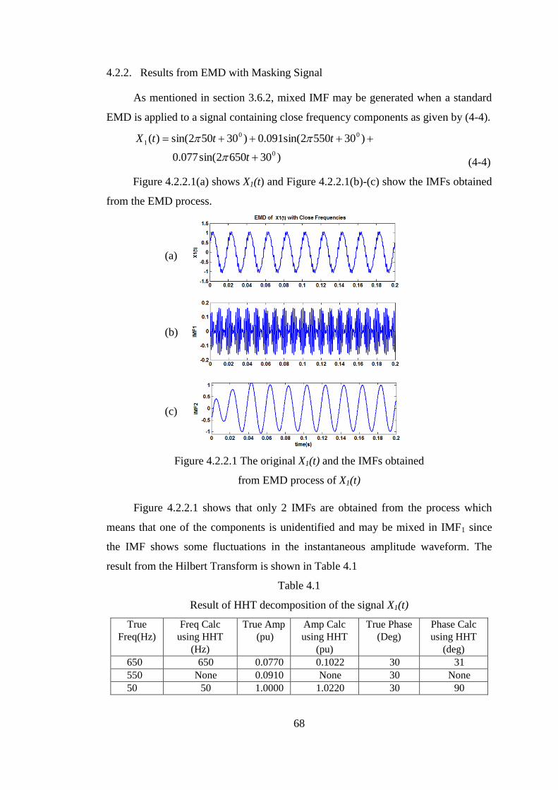
68
4.2.2. Results from EMD with Masking Signal
As mentioned in section 3.6.2, mixed IMF may be generated when a standard
EMD is applied to a signal containing close frequency components as given by (4-4).
)306502sin(077.0
)305502sin(091.0)30502sin()(
0
00
1
t
tttX
(4-4)
Figure 4.2.2.1(a) shows X1(t) and Figure 4.2.2.1(b)-(c) show the IMFs obtained
from the EMD process.
Figure 4.2.2.1 The original X1(t) and the IMFs obtained
from EMD process of X1(t)
Figure 4.2.2.1 shows that only 2 IMFs are obtained from the process which
means that one of the components is unidentified and may be mixed in IMF1 since
the IMF shows some fluctuations in the instantaneous amplitude waveform. The
result from the Hilbert Transform is shown in Table 4.1
Table 4.1
Result of HHT decomposition of the signal X1(t)
True
Freq(Hz)
Freq Calc
using HHT
(Hz)
True Amp
(pu)
Amp Calc
using HHT
(pu)
True Phase
(Deg)
Phase Calc
using HHT
(deg)
650 650 0.0770 0.1022 30 31
550 None 0.0910 None 30 None
50 50 1.0000 1.0220 30 90
(a)
(b)
(c)

69
Table 4.1 shows that the EMD process has succesfully extracted the 650 Hz
and 50 Hz components. However, the 550 Hz component is not identified by the
EMD algorithm.
To overcome the problem, The EMD with masking signal method is then
used to decompose X1(t). To estimate the appropriate masking signal frequency for
the separation of components mixed in IMF1, the Hilbert Transform is used to obtain
the mean value of instantaneous amplitude, frequency and phase of IMF1 as shown in
Figure 4.2.2.2(b)-(d)
Figure 4.2.2.2. The Hilbert Transform of IMF1 of X1(t).
The waveform of IMF1 in Figure 4.2.2.2 shows more clearly that the IMF is
mixed which can be seen from the fluctuations of the instantaneous amplitude and
the instantaneous frequency waveform. To resolve the mode mixing issue, a masking
signal frequency is then estimated by using the formula given in (4-1) which results
in = 879 Hz. The mean value of instantaneous amplitude of IMF1 is 0.1045 p.u. as
shown in Figure 4.2.2.2(c) which is then used by the formula given by (4-2) to
construct the masking signal q(t) =0.1672 sin (2π 1054.8 ).
When the masking signal is applied to the original signal X1(t) according to
step 4 of the algorithm, the first IMF of x+(t) and the first IMF of x−(t) denoted by
IMF+ and IMF- respectively are shown in Figure 4.2.2.3 as follows :
a)
b)
c)
d)
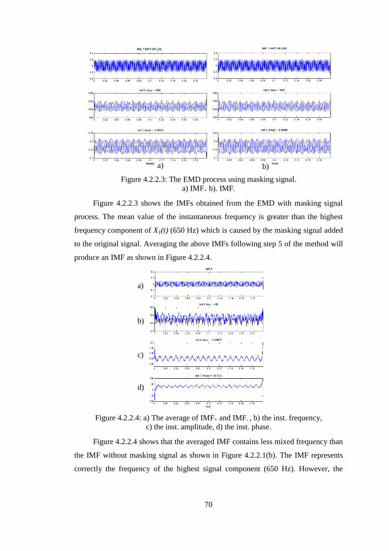
70
Figure 4.2.2.3: The EMD process using masking signal.
a) IMF+ b). IMF-
Figure 4.2.2.3 shows the IMFs obtained from the EMD with masking signal
process. The mean value of the instantaneous frequency is greater than the highest
frequency component of X1(t) (650 Hz) which is caused by the masking signal added
to the original signal. Averaging the above IMFs following step 5 of the method will
produce an IMF as shown in Figure 4.2.2.4.
Figure 4.2.2.4: a) The average of IMF+ and IMF- , b) the inst. frequency,
c) the inst. amplitude, d) the inst. phase.
Figure 4.2.2.4 shows that the averaged IMF contains less mixed frequency than
the IMF without masking signal as shown in Figure 4.2.2.1(b). The IMF represents
correctly the frequency of the highest signal component (650 Hz). However, the
a) b)
a)
b)
c)
d)

71
amplitude of the IMF 0.0398 p.u is smaller than the actual amplitude for 650 Hz
component specified as 0.077 p.u.
The IMF is taken as the first IMF of the process which is then subtracted from
the original signal X1(t) to obtain the residue. The original signal, IMF1 and the
residue are shown in Figure 4.2.2.5
Figure 4.2.2.5 The original signal X1(t), IMF1 and the residue after iteration 1
Figure 4.2.2.5 shows that the residue is still above the specified threshold.
Therefore, according to step 8 of the algorithm, the residue is considered as the
signal x(t) to be processed and the process is then repeated.
The IMFs obtained from the whole decomposition process using the EMD with
masking signal are shown in Figure 4.2.2.6.
Figure 4.2.2.6 The EMD with masking signal process of X1(t)

72
Figure 4.2.2.6 shows that the method has succesfully identified all the
components of the signal containing close frequency. The waveforms of the IMFs are
less mixed with other frequency which demonstrates the advantage of using the
masking signal with the EMD process. However, the use of masking signal does not
guarantee that the IMF obtained from the process will be free from mixing with other
frequency. For example, the waveform of IMF2 in Figure 4.2.2.6 clearly indicates
that it is a modulation of more than one frequency components.
Further, all IMFs in Figure 4.2.2.6 show the existence of end effect problem at
both ends of their waveforms. The error at both ends of the IMF may propagate to
the interior of the data span that may corrupt the subsequent lower frequency IMFs
[45].
The results from the Hilbert Transform of the IMFs are shown in Table 4.2.
Table 4.2 The results of HT of the IMFs from EMD process of X1(t)
Amp
(p.u)
Freq
(Hz)
Phase
(deg)
IMF1 0.0399 650 30.14
IMF2 0.0863 550 29.93
IMF3 0.9958 50 29.99
IMF4 0.0208 28 128.80
Table 4.2 shows that all the frequencies and the phase angles of the signal
components have been detected correctly. However, the amplitude of each IMF does
not show an accurate decomposition result since all the harmonic (550Hz and 650
Hz) amplitudes are smaller than the actual values specified in (4-5), particularly for
IMF1.
4.2.3. EMD with Masking Signal and FFT method [46]
While the algorithm described in section 4.2.1 estimates the frequency of
masking signal using an empirical formula, another algorithm is proposed [46] to use
FFT to guide the construction of the masking signal. The FFT is applied to identify
the frequency and amplitude of the signal components which are then used to
construct appropriate masking signal to help the EMD process for the decomposition
of the signal containing close frequencies.

73
The algorithm is described as follows [46]:
1. Apply FFT to the signal being analysed, x(t), to estimate its frequency
components , f1, f2, f3,.... fn where f1 < f2 < f3.... < fn.
2. Starting from the highest frequency, for every fk, k = n, n-1, n-2, ...2,
construct masking signals, maskk, = Mk x sin(2π(fk + fk-1)t). It is
suggested to use Mk as 5.5 x amplitude of fk obtained in FFT spectrum.
The value of Mk is empirical.
3. Compute two signals x(t) + maskk and x(t) – maskk. Apply EMD to both
signals to obtain their first IMFs, IMF+ and IMF-.
4. IMFk is defined as (IMF+ + IMF-) / 2. The averaging step will cancel out
the positive and negative instances of the masking signal leaving only the
portion of the signal at frequency fk.
5. Each IMF obtained is assumed as a modulation of 2 sinusoids. To
identify the sinusoids, apply the demodulation process to IMFk to obtain
the amplitude, frequency and phase of these sinusoids which may mix in
IMFk.
A fluctuating IMF indicates that the signal contains a mixture of more
than one sinusoid. The waveform is similar to an AM (Amplitude
Modulation) signal usually used in radio communication. The AM signal
can be produced from an original signal (which is usually of lower
frequency) and modulate (multiply) it by another signal. A demodulation
process is the reverse of the modulation process which means that it
basically works to obtain the components of the modulated signal.
6. Create two sinusoidal representations of IMFk denoted by ck(t) using the
amplitudes, frequencies and phase angles of the sinusoids obtained from
the demodulation process.
7. Compute the residue, rk(t) = x(t) – ck(t) then replace x(t) with rk(t).
8. Perform steps 3 – 7 iteratively using the next masking signals and
replacing x(t) with the residue obtained until n-1 IMFs containing
frequency components f2, f3,.... fn are extracted. The nth
residue rn(t) will
contain the remaining component f1.
9. Compute the residue, rk(t) = x(t) – ck(t)

74
10. If the residue, rn(t), is below a threshold value of error tolerance (0.5% of
the maximum value of the original signal), stop the process. Otherwise
replace the signal x(t) with rn(t) and repeat steps 1 – 9 on the new x(t), to
obtain the next IMF and a new residue.
4.2.4. Results from EMD with Masking Signal and FFT method
A simple test is also made to see the performance of the method to decompose
the same PQ signal containing close frequency specified in section 4.2.2 as follows:
)306502sin(077.0
)305502sin(091.0)30502sin()(
0
00
1
t
tttX
(4-5)
To decompose X1(t) by using the technique, the FFT is carried out first to
identify the amplitudes and frequencies of the harmonic components of X1(t). The
amplitude Mk and frequency of masking signal are then calculated from the
highest to the lowest frequency component as shown in Table 4.3.
Table 4.3
The calculated masking signals
maskk
k Mk (p.u) (Hz)
3 0.424 1200
2 0.5005 600
Each of the masking signals shown in Table 4.3 is used to help the EMD
process to reduce the mixing of the close frequency components in the same IMF.
In the first iteration (k = 3) of the process, the mask3 masking signal is used to
obtain IMF+ and IMF- shown in Figure 4.2.4.1:
Figure 4.2.4.1. The EMD process using masking signal and FFT at iteration 1 (k = 3)
a) IMF+ , b) IMF-
a) b) b)

75
Averaging the above IMFs following step 4 of the method results an IMF as
shown in Figure 4.2.4.2 (a). The Hilbert Transform of the averaged IMF is shown in
Figure 4.2.4.2 (b)-(d).
Figure 4.2.4.2.: a) The average of IMF+ and IMF- for k=3,
b) the inst. amplitude, c) the inst. frequency, d) the inst. phase.
Figure 4.2.4.2(a) shows that the averaged IMF contains less mixed frequency.
The mean value of the instantaneous frequency obtained from HT of the IMF, as
shown in Figure 4.2.4.2 (b), represents correctly the frequency of the highest signal
component (650 Hz). However, the mean value of the instantaneous amplitude
waveform obtained from HT of the IMF shown in Fig. 4.2.4.2 (c) is 0.0357 p.u,
which is smaller than the actual amplitude for 650 Hz component specified as 0.077
p.u.
According to step 5 of the algorithm, each IMF obtained from the averaging
process is considered as a mixture of a dominant high frequency component, along
with a remnant lower frequency component. A demodulation process is therefore
required to further identify the components of the IMF.
The demodulation technique used in the algorithm basically assumes that the
IMF contains two sinusoids [46], which can be demodulated by using parametric
methods such as MUSIC algorithm to estimate the amplitudes, frequencies and
phases of these sinusoids. By applying the demodulation process to the IMF shown
in Figure 4.2.4.2(a), the components are obtained as given by Table 4.4 :
a)
b)
c)
d)

76
Table 4.4
The result of demodulation process of IMF from iteration 1, k=3
Amp
(p.u) Freq
(Hz) Phase
(deg)
0.0126 550 20
0.0340 650 30
Table 4.4 shows that the demodulation process has identified 550Hz
component which is mixed with the dominant 650 Hz component in IMF1. The 550
Hz component was not detected by the Hilbert Transform as shown in Figure 4.2.4.2.
Table 4.4 demonstrates the advantage of the EMD using masking signal and FFT
over the original EMD using masking signal only, which does not perform any post
processing of the resulting IMF. Further, the detected sinusoids in the mixed IMF can
be used to represent the IMF as a two sinusoidal representations c3(t) which are free
from the inaccuracy caused by the end effect issue. These representation can then be
subtracted from the original signal, instead of subtracting the original IMF, to obtain
more accurate result.
The detected sinusoids c3(t) from Table 4.4 are then subtracted from the
original signal to obtain the residue r3(t). Since k is still greater than 2, the residue is
then considered as the new signal to be processed x(t) and the process is repeated
from step 3 to step 7.
The second iteration is performed by using the next masking signal (k=2) to
obtain the next IMF+ and IMF- which are then averaged and demodulated. The result
from iteration 2 is shown in Table 4.5.
Table 4.5
The result of demodulation process of IMF from iteration 2, k=2
Amp
(p.u) Freq
(Hz) Phase
(deg)
0.0774 550 30
0.042 650 30
The result in Table 4.5 is used to create the sinusoidal representation c2(t)
which is then subtracted from the signal x(t) to obtain the next residue r2(t).
According to step 8 of the algorithm, when two IMFs contain frequency
components of 550 Hz and 650 Hz have been subtracted from the signal consists of 3
components as given by (4-5), the final residue r2(t) will contain the remaining

77
fundamental component 50 Hz. The Hilbert Transform can then be used straight
away to obtain the instantaneous amplitude, frequency and phase of r2(t) as shown in
Table 4.6.
Table 4.6
The residue after iteration 2
Amp
(p.u) Freq
(Hz) Phase
(deg)
1 50 30
The detected amplitude, frequency and phase in Table 4.6 is then subtracted
from the signal to obtain the new residue. The signal reconstructed from detected
components, X1(t) and the residue of the process is shown in Figure 4.2.4.3
Figure 4.2.4.3 The original signal X1(t), reconstructed signal, and the residue
Figure 4.2.4.3 shows that the reconstructed signal is quite close to the original
signal. However, the residue is still greater than the specified threshold (0.5% of the
maximum value of the original signal), and therefore more iterations are required to
obtain more accurate result.
The process is then repeated by applying FFT to the residue in the next
iterations. The whole result of the algorithm is shown in Table 4.7.
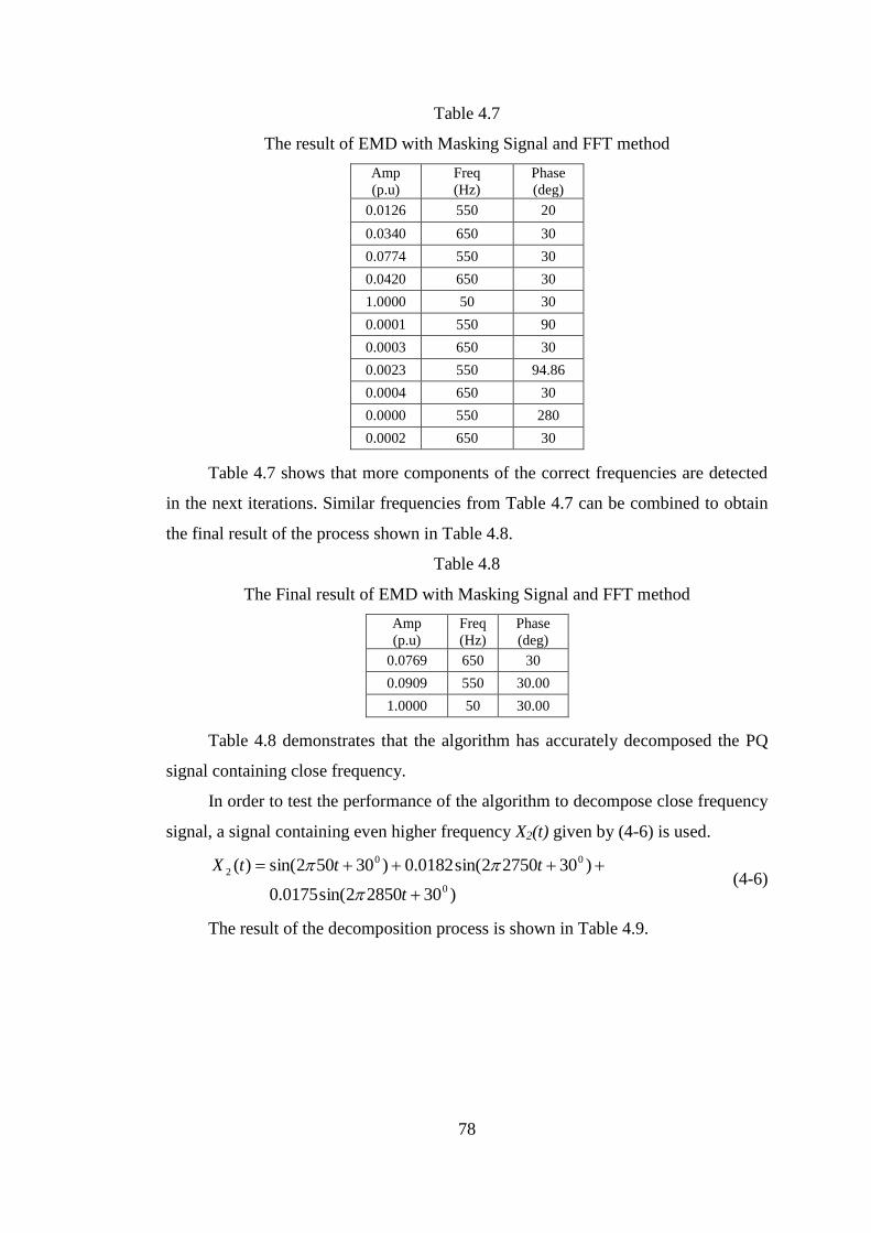
78
Table 4.7
The result of EMD with Masking Signal and FFT method
Amp
(p.u)
Freq
(Hz)
Phase
(deg)
0.0126 550 20
0.0340 650 30
0.0774 550 30
0.0420 650 30
1.0000 50 30
0.0001 550 90
0.0003 650 30
0.0023 550 94.86
0.0004 650 30
0.0000 550 280
0.0002 650 30
Table 4.7 shows that more components of the correct frequencies are detected
in the next iterations. Similar frequencies from Table 4.7 can be combined to obtain
the final result of the process shown in Table 4.8.
Table 4.8
The Final result of EMD with Masking Signal and FFT method
Amp
(p.u)
Freq
(Hz)
Phase
(deg)
0.0769 650 30
0.0909 550 30.00
1.0000 50 30.00
Table 4.8 demonstrates that the algorithm has accurately decomposed the PQ
signal containing close frequency.
In order to test the performance of the algorithm to decompose close frequency
signal, a signal containing even higher frequency X2(t) given by (4-6) is used.
)3028502sin(0175.0
)3027502sin(0182.0)30502sin()(
0
00
2
t
tttX
(4-6)
The result of the decomposition process is shown in Table 4.9.

79
Table 4.9
The result of EMD with masking signal and FFT of X2(t)
Amp
(p.u)
Freq
(Hz)
Phase
(deg)
0.0089 2750 30
0.0106 2850 30
0.0092 2750 30
0.0068 2850 30
1 50 30
Similar frequencies can be combined to obtain the final result as shown in
Table 4.
Table 4.10
The Final result of EMD with masking signal and FFT on X2(t)
Amp
(p.u) Freq
(Hz) Phase
(deg)
0.0175 2850 30
0.0181 2750 30
1 50 30
Table 4.10 demonstrates that the algorithm has successfully decomposed signal
X2(t) which containing higher and closer frequency by using masking signal and
FFT. The decomposition result shows the accuracy of the EMD with masking signal
and FFT method over the EMD with masking signal only.
However, the EMD process using masking signal and FFT algorithm may not
be efficient, since the use of FFT is required to guide the masking signal estimation.
If one already has the amplitude, frequency and phase solution for each component
from FFT, why further work is needed by using HHT?
Further, the use of masking signal does not guarantee that the IMF obtained
will not be mixed with other frequency component [46] and therefore the
demodulation process using parametric method is required to identify the component
of the (still mixed) IMF by assuming that the IMF consists of 2 sinusoids. If one
knows exactly the total number of components in the original signal, a
decomposition process using parametric method (such as MUSIC algorithm) can be
applied directly to decompose the signal. The difficulty lies in the fact that the total
number of harmonic components is usually unknown.

80
4.3. The proposed Iterative HHT
As described in section 3.6.2, the HHT has been found to have difficulty in
resolving waveforms containing components with close frequencies with a ratio of
less than two. Although efforts have been made to resolve the problem by using the
EMD with masking signal [6] and EMD with masking signal and FFT [46], there are
still some issues with the methods.
In the EMD with masking signal method [6], the IMFs obtained from the
process suffer from the end effect problem which causes inaccuracies at both ends of
the IMFs. When the error is processed further by the EMD algorithm, it may
propagate to the inner part of the data span which can corrupt the next lower
frequency IMFs.
In EMD with masking signal and FFT method, the FFT needs to be carried out
to correctly calculate the masking signal frequency. However it appears that there is
a duplication of work in doing this because the FFT can already perform the
decomposition process.
In order to perform more efficient computation of EMD, a modified EMD
technique is proposed in this research. The proposed method uses an iterative process
of HHT to estimate the signal components and therefore is referred to as the iterative
HHT [47].
Since the application of EMD to the signal containing close frequency usually
produce mixed IMF, appropriate steps in the proposed method need to be carried out
to utilize the mixed IMF in the decomposition process. The stopping criteria may
need to be adjusted to obtain a correct mean value of the instantaneous frequency.
Experiments carried out in the research has found that the following stopping criteria
(or smaller) should be used (1 = 0.005, 2 =0.05 and tol= 0.005).
Each mixed IMF obtained from the EMD process of a signal containing close
frequency components can be assumed as a combination of a dominant high
frequency component, along with a remnant lower frequency component [46]. While
the IMF is still mixed, The Hilbert Transform of the IMF generally produce the
instantaneous frequency of the IMF with the mean value equals to the frequency of
the dominant component.
Therefore, in this approach, a sinusoidal representation of the dominant
component is then created by using the mean value of the instantaneous frequency,

81
amplitude and phase of the first IMF. Although the value of instantaneous amplitude
and phase angle of the IMF may not be accurate, they can be calculated iteratively to
improve the accuracy of the result.
The sinusoidal representation of the first IMF is then subtracted from the
original signal and the process is then repeated. Any error obtained during the
calculation in any of these IMFs can be recovered in the succeeding iterative steps
[47].
Since the highest frequency component has been taken out from the original
signal in the first iteration, the lower frequency component can be found more easily
in the next iteration by applying EMD process to the residue.
In this way, the issue of mixed IMFs obtained from the EMD process of a
signal containing close frequency components with ratio of the signal frequency
much less than 2 is resolved. The proposed method does not require any treatment
(such as by introducing masking signal) to make the IMF less mixed or to estimate
the components in the mixed IMF by using any extra technique such as demodulation
process.
The proposed iterative HHT differs from the standard HHT process in two
important respects [38].
First, in the standard HHT all of the obtained IMFs are taken as the final
decomposition result. Therefore, no more calculation is needed. The HT is then
performed on these IMFs. In the proposed iterative method, at each iteration only the
first IMF is taken from each EMD process, then the HT is applied to that IMF to
obtain the sinusoidal representation of the IMF. The sinusoidal representation is then
subtracted from the signal. Therefore, further calculation is needed to repeat the
process on the remainder.
Second, the standard HHT uses the original IMF waveform obtained from the
sifting process to be subtracted from the signal before doing the next sifting in the
EMD algorithm, despite the fact that the IMF may be mixed. In the proposed
iterative method, at each iteration, the IMFs are represented by pure sinusoids whose
amplitude, frequency and phase are obtained from the mean values of the
instantaneous amplitude, frequency and phase given by the HT. The errors in the
calculated amplitude and phase angle of the sinusoidal representation of the signal
components can be corrected as the iterative process progresses.

82
The steps for the iterative HHT of a signal x(t) are described as follows:
1. Find the first IMF using the standard EMD process of x(t).
2. Use the HT to approximate the instantaneous frequency, amplitude and
phase of the first IMF. These approximation are then used to create the
sinusoidal representation of the IMF given by:
P(t) = sin(2π t + ) (4-7)
Where:
P(t) = sinusoidal representation of the first IMF
= approximated amplitude of the first IMF
= approximated frequency of the first IMF
= approximated phase angle of the first IMF
Since the IMF usually contain inaccuracies at both ends as shown in
section 3.4.1 and Figure 3.4.1.1, the approximated amplitude, frequency
and phase are taken by averaging the 10% - 90% length of the
instantaneous amplitude, frequency and phase data points obtained from
the HT of the IMF.
3. Subtract the sinusoidal representation of the first IMF from the original
signal to obtain the residue, r(t)
r(t) = x(t) - ( ) (4-8)
4. Steps 1-3 are repeated on r(t) until the amplitude of the first IMF reaches
a low threshold value. The smaller the threshold, the longer the program
will keep going to decompose and subtract detected components from the
original signal. From experience, a threshold of 0.5% of the maximum
value of the simulated signal has been found to be sufficient to obtain an
accurate result. However, for a measured signal, the threshold needs to be
increased to 3% to take the noise in the signal into account [47].
5. In the iterative HHT method, it is possible that similar frequencies are
obtained during the iterative process of decomposition. For each
frequency fk, obtained in the Iterative HHT process, the sinusoidal
representation associated with that frequency can be added together as
given in (4-9) and then the Hilbert Transform is applied to obtain the

83
amplitude, frequency and phase of that frequency component. These
sinusoids are then sorted by frequency.
Rk = sin(2π t + ) + sin(2π t +
)+.......
..... sin(2π t +
) (4-9)
4.4. Results from the Iterative HHT
To evaluate the performance of the proposed method, the Iterative HHT is then
tested to decompose the stationary signal X1(t) given in (4-5). The result of the first
iteration is shown in Figure 4.4.1
Figure 4.4.1 The first IMF from iteration 1 of the IHHT process on X1(t)
Figure 4.4.1 shows the first IMF from iteration 1 of the IHHT process on X1(t),
which contains mixed frequencies due to the close frequency components which
were not separable by the EMD process of the signal. The mean value of the
instantaneous amplitude 0.1047 p.u is also higher than the specified value 0.0769 p.u
which indicates that the IMF contains other signal components.
However, the mean value of instantaneous frequency of the dominant
component of IMF1 is correctly identified as 650 Hz, which is the most important
thing at this stage since the next iteration will be able to correct the error in
amplitude and phase angle value. The Hilbert Transform of the first IMF at the first
iteration is shown in Table 4.11.
Table 4.11
The HT of IMF1 at iteration 1
Amp
(p.u) Freq
(Hz) Phase
(deg)
0.1047 650 29.97

84
A sinusoidal representation is then constructed based on the mean value of the
instantaneous amplitude, frequency and phase shown in Table 4.11. The sinusoid is
then subtracted from the original signal to obtain the first residue r1(t) which will
then be considered as the new signal to be processed in the second iteration. The
result of the second iteration is shown in Figure 4.4.2.
Figure 4.4.2 The first IMF from iteration 2 of the IHHT process on X1(t)
Figure 4.4.2 shows the first IMF from iteration 2 which looks a bit mixed. The
mean value of the instantaneous amplitude 0.093 p.u is also higher than the specified
value 0.091 p.u. The mean value of the instantaneous frequency is correctly
identified as 550 Hz. The Hilbert Transform of the first IMF at iteration 2 is shown
in Table 4.12.
Table 4.12
The Hilbert Transform of IMF1 at iteration 2
Amp
(p.u) Freq
(Hz) Phase
(deg)
0.093 550 30.05
A sinusoidal representation is then constructed based on the mean value of the
instantaneous amplitude, frequency and phase shown in Table 4.12. The sinusoid
constructed from Table 4.12 is then subtracted from the signal being analysed to
obtain the second residue r2(t) which will then be considered as the new signal to be
processed in the 3rd
iteration, the process is iteratively repeated until the threshold is
reached. The whole result of the IHHT process on signal X1(t) is shown in Table
4.13.

85
Table 4.13
The result of IHHT process on X1(t)
iteration Amp
(p.u) Freq
(Hz) Phase
(deg)
1 0.105 650 29.98
2 0.093 550 30.05
3 0.028 650 209.81
4 1.000 50 30.00
Table 4.13 shows that some of the sinusoids obtained have the same frequency
value. The sinusoids of the same frequency are then combined to obtain the final
result as shown in Table 4.14.
Table 4.14
Final result of IHHT process on X1(t)
True
Freq
(Hz)
Freq
Calc
using
IHHT
(Hz)
True
Amp
(pu)
Amp
Calc
using
IHHT
(pu)
True
Phase
(deg)
Phase
Calc
using
IHHT
(deg)
650 650 0.077 0.077 30 30.04
550 550 0.091 0.093 30 30.05
50 50 1.000 1.000 30 30.00
Table 4.14 shows the final results of the Iterative HHT for the stationary signal
X1(t) which demonstrates that this process can decompose the signal correctly.
The Iterative HHT is also tested to decompose the stationary signal containing
higher frequencies X2(t) given in equation (4-6). The result of the first iteration is
shown in Figure 4.4.3.
Figure 4.4.3 The first IMF from 1st iteration of the IHHT process on X2(t).

86
Figure 4.4.3 shows the first IMF from iteration 1 of the IHHT process on X2(t),
the mean value of instantaneous frequency is correctly identified as 2850 Hz, the
mean value of the instantaneous amplitude and phase angle are identified as 0.018
p.u and 300 respectively. The Hilbert Transform of the IMF is shown in Table 4.15.
Table 4.15
The HT of IMF1 at iteration 1
Amp
(p.u) Freq
(Hz) Phase
(deg)
0.023 2750 30.3
A pure sinusoid is then constructed based on the mean value of the
instantaneous amplitude, frequency and phase shown in Table 4.15. The sinusoid is
then subtracted from the original signal to obtain the first residue r1(t) which will
then be considered as the new signal to be processed in the second iteration. The
result of the second iteration is shown in Figure 4.4.4.
Figure 4.4.4 The first IMF from 2nd
iteration of the IHHT process on X2(t).
Figure 4.4.4 shows the first IMF from iteration 2 of the IHHT process on X2(t),
the mean value of instantaneous frequency is correctly identified 2750 Hz. The mean
value of the instantaneous amplitude and phase angle are identified as 0.0185 p.u.
and 300 respectively. The Hilbert Transform of the IMF is shown in Table 4.16.
Table 4.16
The HT of IMF1 at iteration 2
Amp
(p.u) Freq
(Hz) Phase
(deg)
0.0179 2850 29.99
A pure sinusoid is then constructed based on the mean value of the
instantaneous amplitude, frequency and phase shown in Table 4.16. The sinusoid is

87
then subtracted from the signal being analysed to obtain the second residue r2(t)
which will then be considered as the new signal to be processed in the 3rd
iteration,
the process is iteratively repeated until the threshold is reached. The whole result of
the IHHT process on signal X2(t) is shown in Table 4.17.
Table 4.17
The result of IHHT process on X2(t)
iteration Amp
(p.u)
Freq
(Hz)
Phase
(deg)
1 0.023 2750 30.28
2 0.018 2850 29.99
3 0.005 2750 211.35
4 1 50 30.00
Table 4.17 shows that some of the sinusoids obtained have the same frequency
value. The sinusoids of the same frequency are then combined to obtain the final
result as shown in Table 4.18.
Table 4.18
Final result of IHHT process on X2(t)
True
Freq
(Hz)
Freq
Calc
using
IHHT
(Hz)
True Amp
(pu)
Amp Calc
using
IHHT
(pu)
True
Phase
(deg)
Phase
Calc
using
IHHT
(deg)
2850 2850 0.0175 0.0179 30 29.99
2750 2750 0.0182 0.0182 30 30.01
50 50 1.000 1.000 30 30.00
Table 4.18 shows the final results of the Iterative HHT for the signal X2(t)
which demonstrates that the proposed method of successively subtracting sinusoidal
representation of the first IMF instead of the original IMFs (which is used in the
standard HHT) has led to greater accuracy when dealing with harmonic signals.
To examine the performance of the proposed method, the standard HHT and
the proposed iterative HHT are then tested to decompose various combinations of
harmonic signal from 1 to 4 harmonic components. To do the test, a harmonic signal
with n components is constructed [38] as given by (4-10) :
))1(2sin()1(
...))(2sin()(
)2sin()(
1
21
nftnknk
A
ftkk
AftAtS
(4-10)

88
Where :
A = the amplitude of the fundamental signal
f = 50 Hz
k(m) = 3,5,7,9..., for m=1,2,3,4,....
= phase in radians
= constant offset
For example, a signal containing 50, 350,450,550 Hz will have n=3 since there
are three harmonics (7th
, 9th
and 11th
), =3 since k(3) = 7, followed by k(4) = 9 and
k( +n-1) = k(5) = 11. So the signal will be of the form given by (4-11):
)112sin(11
)92sin(9
...)72sin(7
)2sin()(
43
21
ftA
ftA
ftkA
ftAtS
(4-11)
In the research, all of the harmonic signals analysed contain the fundamental
component with frequency f at 50 Hz and one to four other harmonic components.
The test signals are sampled at 30 kHz over the range 50 Hz to 4950 Hz.
To see the effect of the stopping criteria, different stopping criteria (0.1 x
default value and 0.01 x default value) are used. The results are shown in Table 4.19
and Table 4.20.
Table 4.19
Separation of Harmonic Signals using standard HHT
Number of
harmonic
components (n)
Frequencies separated corectly
Stopping criteria : 0.1x default Stopping criteria : 0.01x default
1 50, 150 Hz to 50, 4950 Hz 50, 150 Hz to 50, 4950 Hz
2 50, 150, 250 to 50, 450, 550 Hz 50, 150, 250 to 50, 850, 950 Hz
3 50, 150, 250, 350 Hz only 50, 150, 250, 350 Hz to
50, 350, 450, 550 Hz
4 50, 150, 250, 350, 450 Hz only 50, 150, 250, 350, 450 Hz to
50, 250, 350, 450, 550 Hz

89
Table 4.20
Separation of Harmonic Signals using Iterative HHT
Number of
harmonic
components (n)
Frequencies separated corectly
Stopping criteria : 0.1xdefault Stopping criteria : 0.01xdefault
1 50, 150 Hz to 50, 4950 Hz 50, 150 Hz to 50, 4950 Hz
2 50, 150, 250 Hz to
50, 4850, 4950 Hz
50, 150, 250 Hz to
50, 4850, 4950 Hz
3
50, 150, 250, 350 Hz to
50, 350, 450, 550 Hz , then
intermittent success
50, 150, 250, 350 Hz to
50, 750, 850, 950 Hz , then
intermittent success
4
50, 150, 250, 350, 450 Hz to 50,
250, 350, 450, 550 Hz then
intermittent success
50, 150, 250, 350, 450 Hz to 50,
450, 550, 650, 750 Hz then
intermittent success
As shown in Table 4.19 and Table 4.20, for n=1, both HHT and IHHT are able
to separate the frequencies upto 50 and 4950 Hz. There is no difference of the
performance of both methods, since the signal does not contain close frequency
components. For signals containing 2 harmonic components (n=2), the Iterative HHT
has successfully separated the components up to 4850, 4950 Hz, while the standard
HHT can separate upto 850, 950 Hz only.
When the number of harmonic components increases, the separation of the
harmonic components is more difficult. However, the Iterative HHT has successfully
separated signals up to the frequency 50, 450, 550, 650, 750 Hz by using the
stopping criteria 0.01 x default. Beyond this point, the separation is not always
successful.
Tables 4-19 and 4-20 also demonstrate the effect of stopping criteria to the
accuracy of the decomposition process. For the stopping criteria used in the Tables,
the smaller the stopping criteria, the more accurate the results are.
4.5. Chapter summary
This chapter has described several techniques to resolve the mode mixing
problem in HHT method. First, the EMD method with masking signal [6] is
discussed. In the algorithm, the masking signal was used to reduce the mixing level
of 2 or more frequencies in the first IMF. The masking signal is constructed from the

90
instantaneous frequency and amplitude data, f1(t) and a1(t) obtained from the Hilbert
Transform of the first IMF. The masking signal is added and subtracted from the
original signal, and the average of the resulting IMFs is then assumed to be the
correct IMF. The method was found to be effective for the signal investigated by the
author. However, the analysis of PQ signal using the method demonstrates that all
IMFs obtained from the process suffer end effect problem. The issue may cause the
propagation of error to the interior of the data span of the particular IMF and may
corrupt the subsequent lower frequency IMFs [45]. In addition, the identified
amplitudes of the components are usually lower than the actual specified amplitudes.
Another method of using EMD with masking signal is by carrying out FFT of
the signal first, from which the frequency and amplitude of the masking signal can be
estimated to reduce the frequency mixing in each IMF [46]. The masking signal is
added and subtracted from the original signal, and the average of the two resulting
IMFs is assumed to be the the correct IMF. A demodulation process is then applied
to estimate the components of each IMF obtained. This method works quite well for
most PQ signal investigated, even one with the high frequency component. Its main
disadvantage is that the FFT has to be calculated first.
Because of the above issues with both methods, a novel Iterative HHT method
is proposed which can carry out the decomposition process without the need of
masking signals or calculating the FFT spectrum of the original signal. In this
method, only the first IMF is used to obtain the instantaneous amplitude, frequency
and phase using the Hilbert Transform. Based on the values of these waveforms, a
sinusoidal representation of the IMF is formed and subtracted from the original
signal. The process is repeated in an iterative fashion, until the amplitude of the
sinusoidal representation is below a certain defined value. The algorithm has been
tested with various PQ harmonic waveforms and it has been found to be effective in
decomposing them even when the signal contains high frequency components.
The purpose of the method discussed in chapter 4 is to improve the
performance of HHT to separate close frequency signal. The separation of such
signal should be examined by using signals containing multiple frequencies which
are close each other. Therefore, harmonics signals with such frequencies are
considered as the most suitable signal for this purpose [6], [7].

91
The proposed method will also be tested to process the non-stationary signal by
first identifying the boundaries of the segments (each of which contains stationary
signal) of the original signal. In the next chapter a new method based on the
Symbolic Aggregate Approximation will be introduced to determine the boundaries
when the signal is non-stationary.

92
CHAPTER 5 THE SAX BASED BOUNDARY
DETECTOR METHOD AND ITERATIVE
HHT TO DECOMPOSE NON-
STATIONARY SIGNAL
5.1. Introduction to SAX
Most PQ signals are non-stationary in nature whose frequency, amplitude, and
phase vary over time. In principle, these could also be assumed as a series of signal
segments, which individually would be stationary [47]. As each signal segment is
potentially composed of a mixture of different elements, the transition from one
segment to the next would be occasioned at an instance where the former mixture is
modified to represent that of the latter segment, such as a change in frequencies
elements and or phases, which in-turn result in manifested different patterns.
Although the standard HHT can automatically obtain the instantaneous
amplitude, frequency, and phase of the components in the non-stationary signal,
uncertainties will occur around the area of a transition. To resolve the problem, a
new method referred to as Symbolic Aggregate Approximation (SAX) analysis is
proposed to identify the instant of changes in the original signal [48]. SAX is a
translation method which works by converting the original time series signal into an
equitable symbolic sequence. The symbolic representation is then processed to
characterize the original signal into various repeating patterns that can be used to
identify particular instants, such as those that relate to sudden change. Once the
instants of sudden changes have been identified, the composite non-stationary signal
could then be divided into a sequence of stationary signals segments. Subsequently,
the HHT and the Iterative HHT can then be applied to decompose each of these
(stationary signal) segments.
5.2. SAX Algorithm
The algorithm was first introduced in 2002 by Patel, Keogh and colleagues
[49], who proposed a symbolic representation which is referred to as SAX (Symbolic
Aggregate ApproXimation) of a time series which can be used for data mining
purposes such as pattern recognition, anomaly detection and data size reduction .
The first step to obtain a SAX representation of a long time series Q of length n
with the elements q1,q2,….qn is to convert the elements of Q to a dimensionality
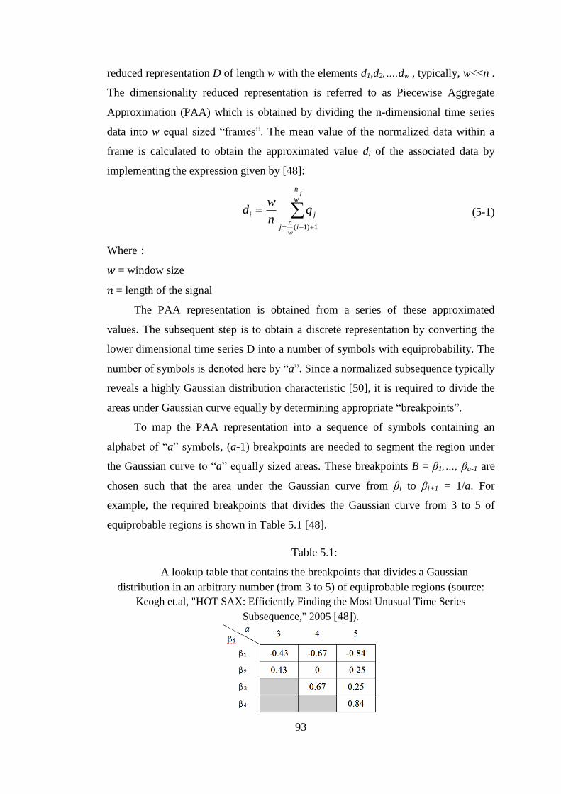
93
reduced representation D of length w with the elements d1,d2,….dw , typically, w<<n .
The dimensionality reduced representation is referred to as Piecewise Aggregate
Approximation (PAA) which is obtained by dividing the n-dimensional time series
data into w equal sized “frames”. The mean value of the normalized data within a
frame is calculated to obtain the approximated value di of the associated data by
implementing the expression given by [48]:
iw
n
iw
nj
ji qn
wd
1)1(
(5-1)
Where :
= window size
= length of the signal
The PAA representation is obtained from a series of these approximated
values. The subsequent step is to obtain a discrete representation by converting the
lower dimensional time series D into a number of symbols with equiprobability. The
number of symbols is denoted here by “a”. Since a normalized subsequence typically
reveals a highly Gaussian distribution characteristic [50], it is required to divide the
areas under Gaussian curve equally by determining appropriate “breakpoints”.
To map the PAA representation into a sequence of symbols containing an
alphabet of “a” symbols, (a-1) breakpoints are needed to segment the region under
the Gaussian curve to “a” equally sized areas. These breakpoints B = β1,…, βa-1 are
chosen such that the area under the Gaussian curve from βi to βi+1 = 1/a. For
example, the required breakpoints that divides the Gaussian curve from 3 to 5 of
equiprobable regions is shown in Table 5.1 [48].
Table 5.1:
A lookup table that contains the breakpoints that divides a Gaussian
distribution in an arbitrary number (from 3 to 5) of equiprobable regions (source:
Keogh et.al, "HOT SAX: Efficiently Finding the Most Unusual Time Series
Subsequence," 2005 [48]).
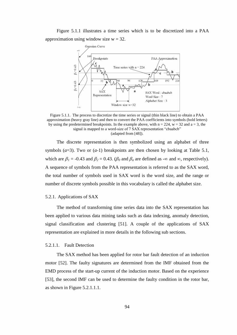
94
Figure 5.1.1 illustrates a time series which is to be discretized into a PAA
approximation using window size w = 32.
Figure 5.1.1. The process to discretize the time series or signal (thin black line) to obtain a PAA
approximation (heavy gray line) and then to convert the PAA coefficients into symbols (bold letters)
by using the predetermined breakpoints. In the example above, with n = 224, w = 32 and a = 3, the
signal is mapped to a word-size of 7 SAX representation “cbaabcb”
(adapted from [48]).
The discrete representation is then symbolized using an alphabet of three
symbols (a=3). Two or (a-1) breakpoints are then chosen by looking at Table 5.1,
which are 1 = -0.43 and 2 = 0.43. (0 and a are defined as - and , respectively).
A sequence of symbols from the PAA representation is referred to as the SAX word,
the total number of symbols used in SAX word is the word size, and the range or
number of discrete symbols possible in this vocabulary is called the alphabet size.
5.2.1. Applications of SAX
The method of transforming time series data into the SAX representation has
been applied to various data mining tasks such as data indexing, anomaly detection,
signal classification and clustering [51]. A couple of the applications of SAX
representation are explained in more details in the following sub sections.
5.2.1.1. Fault Detection
The SAX method has been applied for rotor bar fault detection of an induction
motor [52]. The faulty signatures are determined from the IMF obtained from the
EMD process of the start-up current of the induction motor. Based on the experience
[53], the second IMF can be used to determine the faulty condition in the rotor bar,
as shown in Figure 5.2.1.1.1.

95
Figure 5.2.1.1.1. : The second IMF of the start-up current for a) healthy
machine, b) a machine with one broken bar and c) a machine with two broken bars
(source: P. Karvelis et.al, "An intelligent icons approach for rotor bar fault
detection," 2013 [53])
Figure 5.2.1.1.1 shows that three categories of the rotor bar healthy conditions
(a healthy machine, a machine with one broken bar and a machine with two broken
bars) are used as the target classes of the identification process. Each target class has
a unique pattern of IMF2 obtained from the decomposition process of start-up
current.
To test the proposed method, the start-up currents from a healthy machine and
from a machine with one and two broken rotor bars were recorded. Three different
current transducers are used in the recording process to obtain three recordings for
each faulty condition. The machine start up were performed 10 times for each faulty
condition to obtain 30 recordings for healthy condition, 30 recordings for faulty
condition with one broken bar and 30 recordings for faulty condition with two
broken bars. The recordings are named based on the faulty conditions, sample #1 to
sample #30 are the recordings of healthy machines, sample #31 to sample #60 are the
data of machines with one broken bar, sample #61 to sample #90 are the data of
machines with two broken bars. Each of the second IMF of the data is normalized
and transformed to SAX representations as shown in Figure 5.2.1.1.2
The symbolic representation of the data is used to measure the Euclidean
distance of a particular sample to the other samples. A distance matrix of 30 normal
machines and 60 faulty machines is then obtained and shown in Figure 5.2.1.1.3
a)
b)
c)
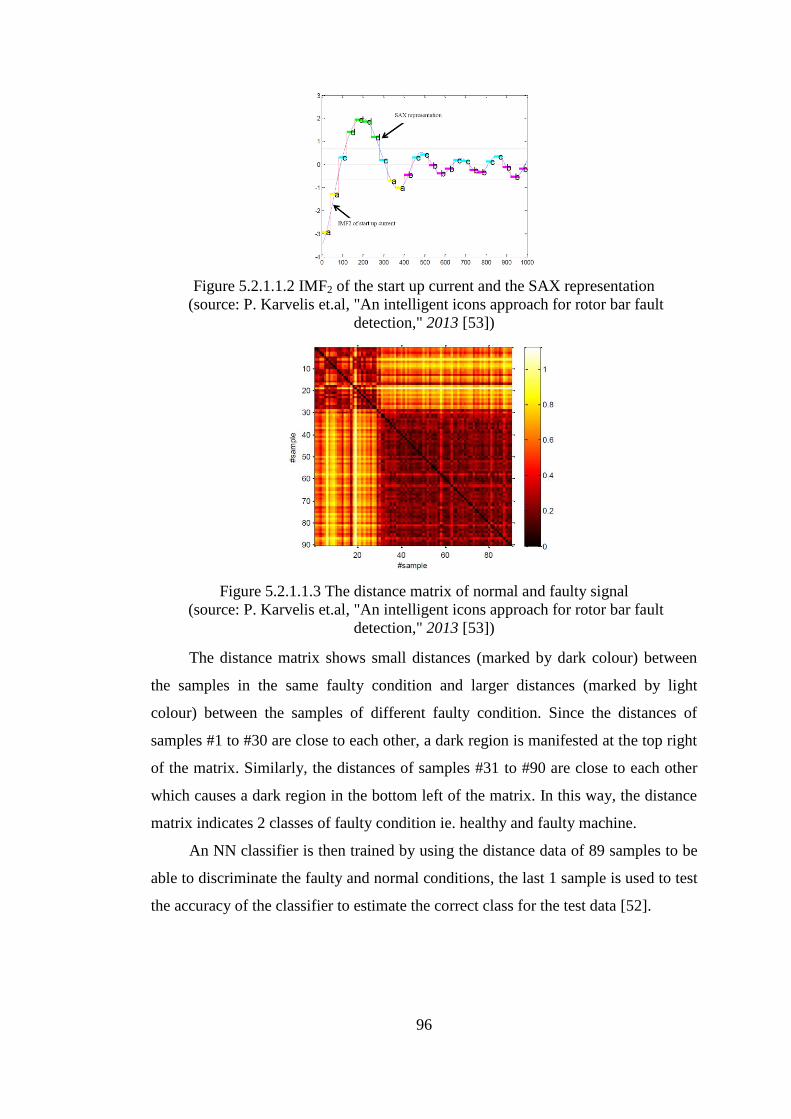
96
Figure 5.2.1.1.2 IMF2 of the start up current and the SAX representation
(source: P. Karvelis et.al, "An intelligent icons approach for rotor bar fault
detection," 2013 [53])
Figure 5.2.1.1.3 The distance matrix of normal and faulty signal
(source: P. Karvelis et.al, "An intelligent icons approach for rotor bar fault
detection," 2013 [53])
The distance matrix shows small distances (marked by dark colour) between
the samples in the same faulty condition and larger distances (marked by light
colour) between the samples of different faulty condition. Since the distances of
samples #1 to #30 are close to each other, a dark region is manifested at the top right
of the matrix. Similarly, the distances of samples #31 to #90 are close to each other
which causes a dark region in the bottom left of the matrix. In this way, the distance
matrix indicates 2 classes of faulty condition ie. healthy and faulty machine.
An NN classifier is then trained by using the distance data of 89 samples to be
able to discriminate the faulty and normal conditions, the last 1 sample is used to test
the accuracy of the classifier to estimate the correct class for the test data [52].

97
5.2.1.2. Data size reduction
Another use of the SAX representation is reported in data size reduction
process to classify electrical load consumption patterns. The load consumption
patterns which is referred to as Representative Load Pattern (RLP) of each consumer
can be represented by using the data points in the time domain or using a reduced
number of features. The study proposes the use of Symbolic Aggregate
Approximation (SAX) method to form the reduced set of features.
The use of the SAX representation to classify electrical load consumption
patterns is clearly simpler than the implementation of principal component analysis
(PCA) or Sammon map on a local board [54]. The SAX representation is more
intuitive for the operators than the PCA or Sammon map outputs.
5.2.1.3. Anomaly Detection
The SAX symbolic representation can also be used to find anomalies
(discords) in ECG signal [48]. By converting the signal to SAX representation, the
time series discords can be found as subsequences of a longer time series that are
maximally different to all the rest of the time series subsequences. Keogh and
colleagues have found in their work that the identified discords coincide with heart
disorder. Figure 5.2.1.3.1 shows an ECG signal with 3 anomalies (discords).
Figure 5.2.1.3.1. An ECG signal with 3 detected anomalies (discords)which exactly
coincides with the heart anomaly (source: Keogh et.al, "HOT SAX: Efficiently Finding
the Most Unusual Time Series Subsequence," 2005.)
Anomalous pattern detection by using the SAX representation is also used in
the assessment of clustered rooftop solar PV impacts in smart grid [55]. Figure
5.2.1.3.2 shows the detection of unusual voltage profile due to distortion by cloud
passing. The signal is converted to a SAX representation which is then characterized
by using a pattern detector to identify the most unusual patterns.

98
Figure 5.2.1.3.2. Detection of unusual voltage profile (source: Alam et.al, "A SAX-
based advanced computational tool for assessment of clustered rooftop solar PV
impacts on LV and MV networks in smart grid,", 2013.)
5.2.2. Determination of window size and alphabet size of the SAX representation
In order to transform the non-stationary signal into an accurate SAX
representation, the window size “w” and alphabet size “a” have to be determined
properly. If a very large value of “w” is chosen, some important details may not be
represented clearly in the SAX representation. Basically, the reduced dimensionality
in the SAX representation should be able to represent the data properly without
loosing any essential feature of the data [56].
For example, a signal S(t) given in (5-2) is transformed to two SAX
representations using alphabet size a = 50. The first representation uses w = 20, while
the second one uses w = 40. The signal changes at sample point no 1040 as shown in
Figure 5.2.2.1.
stttt
stttttS
baab
aaaa
3.0104.0),6502sin(0.092)5502sin(109.0)502sin(2.1
104.00),6502sin(077.0)5502sin(091.0)502sin()(
(5-2)
Figure 5.2.2.1: SAX representation of signal S(t) with alphabet size a = 50.
(a). Using window size w = 20 (b). Using window size w = 40.
Figure 5.2.2.1 (a) shows that the SAX representation with window size 20 can
represent the signal before and after the change at point no 1040 as completely
a) b)
n (data points) n (data points)
Norm
ali
zed
data
Norm
ali
zed
data

99
different words. However, when the window size is increased to 40 as shown in
Figure 5.2.2.1 (b), the SAX representation transforms two or more sub sequences
which are significantly different to a same symbol (in this example, “z” is used to
represent such sub sequences). When a boundary detector algorithm is applied to
such SAX representation, inaccuracies may occur.
On the contrary, if a very small value of “w” is chosen, The SAX
representation may translate insignificant variations (such as the variations due to
noise content in the signal) to different symbols which may cause inaccuracy in the
boundary detection process.
For example, a noisy periodic signal is generated by using the same formula of
the signal S(t) given in (5-2) but now it is added with white gaussian noise with
Signal – To - Noise Ratio (SNR) = 30. The noisy signal is then transformed to a SAX
representation using window size w = 5 as shown in Figure 5.2.2.2.
Figure 5.2.2.2 SAX representation of a noisy signal using w= 5
Figure 5.2.2.2 shows two consecutive cycles in a noisy periodic signal. It is
expected that these two cycles are translated to the same symbolic representation.
However, the choice of the window size “w” = 5 affects the translation process to
obtain inconsistent symbolic representation “676” in former cycle and “775” in the
latter cycle. The inconsistency occurs since the symbolic code is obtained by
averaging the inconsistent noisy data within a short window. A sufficiently longer
window size is needed to let the mean value of the noise content to be very small
which can be neglected to obtain an accurate symbolic representation.
n (data points)
Norm
ali
zed
data
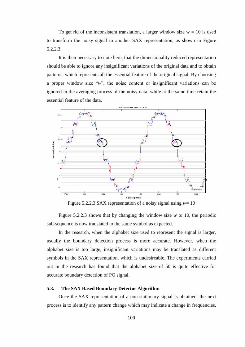
100
To get rid of the inconsistent translation, a larger window size w = 10 is used
to transform the noisy signal to another SAX representation, as shown in Figure
5.2.2.3.
It is then necessary to note here, that the dimensionality reduced representation
should be able to ignore any insignificant variations of the original data and to obtain
patterns, which represents all the essential feature of the original signal. By choosing
a proper window size “w”, the noise content or insignificant variations can be
ignored in the averaging process of the noisy data, while at the same time retain the
essential feature of the data.
Figure 5.2.2.3 SAX representation of a noisy signal using w= 10
Figure 5.2.2.3 shows that by changing the window size w to 10, the periodic
sub-sequence is now translated to the same symbol as expected.
In the research, when the alphabet size used to represent the signal is larger,
usually the boundary detection process is more accurate. However, when the
alphabet size is too large, insignificant variations may be translated as different
symbols in the SAX representation, which is undesireable. The experiments carried
out in the research has found that the alphabet size of 50 is quite effective for
accurate boundary detection of PQ signal.
5.3. The SAX Based Boundary Detector Algorithm
Once the SAX representation of a non-stationary signal is obtained, the next
process is to identify any pattern change which may indicate a change in frequencies,
Norm
ali
zed
data
n (data points)

101
amplitudes or phases of the signal components. The technique to detect the changes
in the signal is referred to as the boundary detector algorithm, which can be
described as follows :
1. Convert the symbols of SAX representation to a numeric alias (for example
“a” = 1, “b” = 2 and so on) to facilitate the comparison process.
2. Find out the cycle length cyc of the periodic signal.
3. Set the base point of searching bsearch equals to cyc+1
4. Set the starting point of the search i equals to bsearch
5. Compare the value of window i to window i-cyc (the window of previous
cycle). A window contains only a number / symbol of SAX representation.
6. If the difference of the numerical value of window i to window i-cyc 1
AND
the difference of the numerical value of window i + 1 to window i-cyc+1
1, mark the window as the change window, then compare the cumulative
sum of the Euclidean distance to a predefined threshold.
7. If the cumulative sum of the Euclidean distances of the previous and current
sub-sequences of a cycle exceeds a predefined threshold, mark the first
point of change as the boundary bnd, set the base point of next search
bsearch equals to bnd + cyc +1 then reset the cumulative sum to zero.
8. If the the cumulative distance does not satisfy step 6, repeat step 5 to 7 on
the next window (i+1).
9. Stop the process if the sliding window i reaches the end of the signal.
5.4. Applying IHHT and SAX-based Boundary Detector to non-stationary
signals
To test the ability of the SAX-based boundary detector, as well as the Iterative
and standard HHT algorithms to decompose a nonstationary harmonic signal
contains close frequency, a couple of examples are described in the following
sections.
5.4.1. Non-stationary PQ waveform with harmonics variations
A non-stationary signal contains variations of harmonic components is given
by (5-3) and shown in Figure 5.4.1.1.

102
stttt
stttt
sttt
tS
cccc
bbbb
aaa
k
3.02.0),3502sin(143.0)2502sin(2.0)502sin(
2.01.0),6502sin(077.0)5502sin(091.0)502sin(
1.00),1502sin(33.0)502sin(
)(
(5-3)
Figure 5.4.1.1. A Non-stationary signal with harmonics variations Sk(t)
The instants of the transitions are specified at t1 = 0.1 s and t2 = 0.2 s. The data
are normalized by first evaluating the mean ( ) and the standard deviation () of the
data series. Each data point is subtracted by and the result is divided by . The
normalized signal is then converted to the SAX representation. This is subsequently
used to detect and resolve where these instants of sudden change occur within the
SAX sequence which, in turn, represents the boundaries of each stationary segment.
Once these have been determined, the stationary signal in each segment is
consequently decomposed using the standard HHT and the Iterative HHT approach.
A window size of 20 (w = 20) is utilized for this signal, that is every 20 sample
points in the original signal will be converted into a window of SAX representation.
The whole time series (here 3000 points) is thus transformed into a SAX sequence of
150 characters (symbols). An alphabet size of 50 symbols (a = 49 breakpoints) is
used. The SAX representation of Sk(t) is shown in Figure 5.4.1.2.

103
Figure 5.4.1.2: the SAX representation of non-stationary signal Sk(t) with
harmonic variations
As successive cycles of the raw signal are translated into the approximated
stream of symbols, any change of the patterns within this temporal sequence become
immediately apparent. The longest common sub sequence (LCCS) of these would
naturally correspond to the cycle.
Since Sk(t) is a periodic signal , the SAX word representation for each period
will be repeated after each cycle if there is no change of the signal component. The
word representing a typical cycle of the signal can then be determined accordingly.
For example, in Figure 5.4.1.2, each cycle is represented as a SAX string of 10
symbols. Having converted the signal into a SAX representation, repeating
subsequences of these symbol patterns (or motifs) will obviously correspond to any
reoccurring stationary cycles of the signal (regular or distorted). Subsequently,
significant pattern changes, will be manifested as changes of these symbol
subsequences.
The advantage of using SAX symbols (rather than instantaneous values), to
collectively form a quantized approximation of the signals numeric range is that any
pattern change is readily detected through the (self) non-matching comparison via a
sliding window, when a cumulative sum of the Euclidean distance of two
corresponding subsequences (at the previous and current cycle respectively) exceeds
a predefined threshold. This is predicated on the Lower Bounding property of SAX,
Norm
ali
zed
data
n (data points)

104
where any such instances in the waveform will correspond to the boundary of
transition for each segment of a non-stationary signal [48].
Subsequently, a boundary detection algorithm is utilized in order to detect and
further establish the boundary times for any differing segments using a cycle-by-
cycle comparison of the SAX numeric values within the word. The boundary can be
identified when a cumulative sum of the Euclidean distance of two corresponding
subsequences (at the previous and current cycle respectively) exceeds a predefined
threshold. At the beginning of the cycle the sum is reset to zero. A threshold of 2.2
have been chosen in this research work. The first boundary is detected at the sample
point n1=51 since it is the first point of change which produce the cumulative sum of
the Euclidean distances of the previous and current sub-sequences exceeded the
threshold as shown in Table 5.2. The next boundary is found at n2=101. These points
in SAX representation coincide with: t1 = 0.1 sec and t2 = 0.2 sec which are the actual
boundaries specified above. The period of each cycle is 0.02 sec in the original
signal.
Table 5.2
The SAX word for two consecutive cycles of Signal Sk(t)
S1(n1) S2(n2) Euclidean
n1
symbol
l1 value n2
symbol
l2 value
Dist
Sum
49 „f‟ 6 39 „f‟ 6 0
50 „l‟ 12 40 „l‟ 12 0
51 „7‟ 34 41 „B‟ 38 4
52 „H 44 42 „I‟ 45 4.12
... ... ... ... ... ... ...
99 „g‟ 7 89 „g‟ 7 0
100 „q‟ 17 90 „q‟ 17 0
101 „A‟ 37 91 „7‟ 34 3
102 „f‟ 42 92 „H‟ 44 3.6
..... ..... ..... ..... ..... ..... .....
Table 5.2 shows how the SAX representation can be processed by a boundary
detector to identify the boundaries of signal Sk(t). The identified boundaries are then
used to segment the signal into 3 segments, each of which contains stationary signal
which can be processed by the standard HHT and the proposed IHHT. Table 5.3

105
shows the results of the signal decomposition using the standard HHT and Table 5.4
shows the results using the proposed Iterative HHT methods.
Table 5.3
Result of HHT decomposition of Signal Sk(t)
0s ≤t<0.10s 0.10 s ≤t<0.20 s 0.20 s ≤t<0.30s
A f φ A f φ A f φ
0.33 150 0.2 0.0997 650 0.0 0.148 350 0
1.0 50 0 0.0189 450 180 1.01 50 3.7
1 50 3.98
Table 5.4
Result of IHHT decomposition of Signal Sk(t)
0s ≤t<0.10s 0.10 s ≤t<0.20 s 0.20 s ≤t<0.30s
A f φ A f φ A f φ
0.33 150 0.2 0.077 650 0.0 0.148 350 0.0
1.0 50 0 0.092 550 0.0 0.2 250 0.1
1.0 50 0.0 1.000 50 2.3
Comparing the result given in Table 5.3 and Table 5.4 to the specified values
given in (5-3) shows that the IHHT is more accurate in decomposing these segments
of non-stationary signal obtained through the SAX – based boundary detector.
5.4.2. Non-stationary PQ waveform with harmonics and sag
A nonstationary signal contains harmonic and sag SL(t) with transition time
close to signal SA(t) in equation (3-15) is used. The instants of the transitions are
specified at t1 = 0.102 sec. and t2 = 0.202 sec, which are different to the specified
boundary points of S(t). The reason of choosing these points is to show the ability of
SAX – based boundary detector to identify correctly the boundary points which are
located between the cycles. Such boundary points cannot be identified accurately by
the windowing technique described in Chapter 3. The components are also modified
from S(t) to contain close frequency like the signal in equation (3-19). The purpose
of the modification is to show the ability of IHHT to decompose close frequency
signal which was not identified accurately by using the standard HHT. The signal
SL(t) is given by equation (5-4) and shown in Figure 5.4.2.1.

106
stttt
stttt
stttt
tS
cccc
bbbb
aaaa
L
3.0202.0),6502sin(077.0)5502sin(091.0)502sin(
202.0102.0),6502sin(062.0)5502sin(073.0)502sin(8.0
102.00),6502sin(077.0)5502sin(091.0)502sin(
)(
(5-4)
Figure 5.4.2.1. Non-stationary signal with harmonics and sag SL(t)
A window size of 10 (w = 10) is utilized for this signal, that is every 10 sample
points in the original signal will be converted into a window of SAX representation.
The whole time series (here 3000 points) is thus transformed into a SAX sequence of
300 characters (symbols). An alphabet size of 20 symbols (a = 19 breakpoints) is
used. The SAX representation of SL(t) is shown in Figure 5.4.2.2.
Figure 5.4.2.2 SAX representation of SL(t)
n (data points)
Norm
ali
zed
data
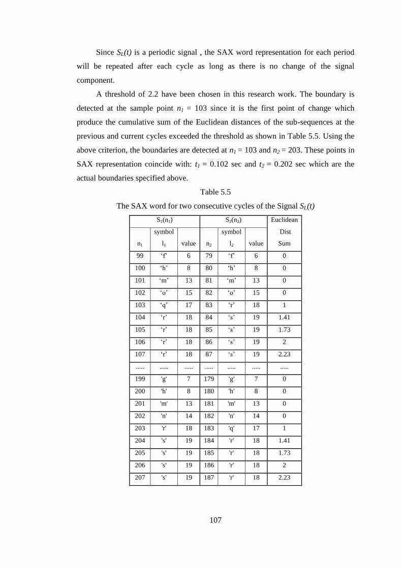
107
Since SL(t) is a periodic signal , the SAX word representation for each period
will be repeated after each cycle as long as there is no change of the signal
component.
A threshold of 2.2 have been chosen in this research work. The boundary is
detected at the sample point n1 = 103 since it is the first point of change which
produce the cumulative sum of the Euclidean distances of the sub-sequences at the
previous and current cycles exceeded the threshold as shown in Table 5.5. Using the
above criterion, the boundaries are detected at n1 = 103 and n2 = 203. These points in
SAX representation coincide with: t1 = 0.102 sec and t2 = 0.202 sec which are the
actual boundaries specified above.
Table 5.5
The SAX word for two consecutive cycles of the Signal SL(t)
S1(n1) S2(n2) Euclidean
n1
symbol
l1 value n2
symbol
l2 value
Dist
Sum
99 „f‟ 6 79 „f‟ 6 0
100 „h‟ 8 80 „h‟ 8 0
101 „m‟ 13 81 „m‟ 13 0
102 „o‟ 15 82 „o‟ 15 0
103 „q‟ 17 83 „r‟ 18 1
104 „r‟ 18 84 „s‟ 19 1.41
105 „r‟ 18 85 „s‟ 19 1.73
106 „r‟ 18 86 „s‟ 19 2
107 „r‟ 18 87 „s‟ 19 2.23
..... ..... ..... ..... ..... ..... .....
199 'g' 7 179 'g' 7 0
200 'h' 8 180 'h' 8 0
201 'm' 13 181 'm' 13 0
202 'n' 14 182 'n' 14 0
203 'r' 18 183 'q' 17 1
204 's' 19 184 'r' 18 1.41
205 's' 19 185 'r' 18 1.73
206 's' 19 186 'r' 18 2
207 's' 19 187 'r' 18 2.23

108
Table 5.5 shows how the SAX representation can be processed by a boundary
detector to identify the boundaries of the non-stationary signal SL(t).
The identified boundaries are then used to segment the signal into 3 segments,
each of which contains stationary signal which can be processed by the standard
HHT and the proposed IHHT. Table 5.6 shows the results of the signal
decomposition using the standard HHT and Table 5.7 shows the results using the
proposed Iterative HHT methods.
Table 5.6
Result of HHT decomposition of signal SL(t)
0s ≤t<0.102s 0.102 s ≤t<0.202 s 0.202 s ≤t<0.30s
A f φ A f φ A f φ
0.105 650 4.1 0.084 650 4.1 0.105 650 4.1
0.009 350 8.3 0.007 350 8.3 0.009 350 8.3
1.000 50 0.0 0.800 50 0.0 1.000 50 0.0
Table 5.7
Result of IHHT decomposition of signal SL(t)
0s ≤t<0.102s 0.102 s ≤t<0.202 s 0.202 s ≤t<0.30s
A f φ A f φ A f φ
0.077 650 0.0 0.061 650 0.0 0.077 650 0.0
0.091 550 0.0 0.073 550 0.0 0.091 550 0.0
1.000 50 0.0 0.800 50 0.0 1.000 50 0.0
Comparing the result given in Table 5.6 and Table 5.7 to the specified values
given in (5-4) shows that IHHT is more accurate in decomposing these segments of
non-stationary signal obtained through SAX – based boundary detector.
5.4.3. Non-stationary PQ waveform with harmonics and swell
The Iterative HHT is also applied to a non-stationary PQ signal SM(t) with
harmonics and swell as given by equation (5-5) and shown in Figure 5.4.3.1.
stttt
stttt
stttt
tS
cccc
bbbb
aaaa
M
3.0208.0),6502sin(077.0)5502sin(091.0)502sin(
208.0106.0),6502sin(0.092)5502sin(109.0)502sin(2.1
106.00),6502sin(077.0)5502sin(091.0)502sin(
)(
(5-5)

109
Figure 5.4.3.1 The original signal SM(t)
The SAX representation of signal SM(t) is then obtained by using a window
size of 10 (w = 10) and alphabet size of 50 symbols (a = 49 breakpoints). The SAX
representation of SM(t) is shown in Figure 5.4.3.2.
Figure 5.4.3.2: The SAX representation of signal SM(t)
The boundary detector is then applied to detect a cumulative distance which
exceeds a threshold of 2.2. The boundary is detected at the sample point n1 = 107
which is the first point of change that produces the cumulative sum of the Euclidean

110
distances of the sub-sequences at the previous and current cycles exceeds the
threshold as indicated in Table 5.8. Using the above criterion, the boundaries are
detected at n1 = 107 and n2 = 209. These points in SAX representation coincide with:
t1 = 0.106 sec and t2 = 0.208 sec which are the actual boundaries specified above.
Table 5.8
The SAX word for two consecutive cycles of Signal SM(t)
S1(n1) S2(n2) Euclidean
n1
symbol
l1 value n2
symbol
l2 value
Dist
Sum
105 „I‟ 45 85 „I‟ 45 0
106 „I‟ 45 86 „I‟ 45 0
107 „K‟ 47 87 „I‟ 45 2
108 „H‟ 44 88 „F‟ 42 2.82
109 „B‟ 38 89 „9‟ 36 3.46
..... ..... ..... ..... ..... ..... .....
208 'H' 44 188 'H' 44 0
209 '9' 36 189 'B' 38 2
210 '5' 32 190 '6' 33 2.23
211 't' 20 191 's' 19 2.45
212 'p' 16 192 'n' 14 3.16
Table 5.8 shows how the SAX representation can be processed by a boundary
detector to identify the boundaries of the non-stationary signal SM(t).
The identified boundaries are then used to segment the signal into 3 segments,
each of which contains stationary signal which can be processed by the standard
HHT and the proposed IHHT. Table 5.9 shows the results of the signal
decomposition using the standard HHT and Table 5.10 shows the results using the
proposed Iterative HHT method.
Table 5.9
Result of HHT decomposition of signal SM(t)
0s ≤t<0.102s 0.102 s ≤t<0.202 s 0.202 s ≤t<0.30s
A f φ A f φ A f φ
0.105 650 4.1 0.126 650 4.1 0.105 650 4.1
0.009 350 8.3 0.011 350 8.3 0.009 350 8.3
1.000 50 0.0 1.200 50 0.0 1.000 50 0.0

111
Table 5.10
Result of IHHT decomposition of signal SM(t)
0s ≤t<0.102s 0.102 s ≤t<0.202 s 0.202 s ≤t<0.30s
A f φ A f φ A f φ
0.077 650 0.0 0.092 650 0.0 0.077 650 0.0
0.091 550 0.0 0.109 550 0.0 0.091 550 0.0
1.000 50 0.0 1.200 50 0.0 1.000 50 0.0
Comparing the result given in Table 5.9 and Table 5.10 to the specified values
given in (5.5) shows that IHHT is more accurate in decomposing these segments of
nonstationary swell signal obtained through SAX – based boundary detector.
5.4.4. Non-stationary PQ waveform with transient
The Iterative HHT is also applied to a non-stationary PQ signal SN(t) with
harmonics and transient as given by equation (5-6). The signal is shown in Figure
5.4.4.1:
stttt
stet
ttt
stttt
tS
cccc
b
t
b
bbb
aaaa
N b
3.0164.0),6502sin(077.0)5502sin(091.0)502sin(
164.0104.0,)20002sin(
)6502sin(077.0)5502sin(091.0)502sin(
104.00),6502sin(077.0)5502sin(091.0)502sin(
)( )104.0(60
(5-6)
Figure 5.4.4.1 The original signal SN(t)

112
Identifying the boundaries of such a signal using cycle by cycle search may not
obtain an accurate result, since the boundaries of the signal pattern is not easily
observed, unlike the sag or swell signal discussed above. An alternative approach is
required to accurately identify the boundary of the signal. According to equation (5-
6), the frequency of the transient signal is significantly higher than the frequencies of
other components of the signal. Therefore, the instantaneous frequency data obtained
from the Hilbert Transform of IMF1 is used to identify the boundaries of the signal.
As shown in Figure 5.4.4.2, the instantaneous frequency plot of IMF1 shows more
obvious boundaries of the signal contains transient SN(t).
Figure 5.4.4.2: The instantaneous frequency plot of IMF1 of SN(t)
A window size of 40 (w = 40) is utilized for this signal, that is every 40 sample
points in the original signal will be converted into a window of SAX representation.
An alphabet size of 10 are used to obtain the SAX representation of the instantaneous
frequency of SN(t) as shown in Figure 5.4.4.3.
Figure 5.4.4.3: The SAX representation of the instantaneous frequency data of IMF1
from EMD process of SN(t)
n (data points)
Norm
ali
zed
da
ta

113
Figure 5.4.4.3 shows that the SAX representation have made the boundary
detection of SN(t) more visible by identifying the level of each window of the
instantaneous frequency plot of the signal. The instant when the transient content of
the signal occurs is indicated by the higher instantaneous frequency value while the
rest of the instantaneous frequency data with lower frequency value indicates the
frequency components without transient content. The difference of the signal patterns
is then utilized by the boundary detector to identify the boundary of the signal.
A boundary detection algorithm is then applied in order to detect and further
establish the boundary times for any differing segments using two consecutive
segments comparison of the SAX numeric values within the word. A window is slid
on each segment to check the Euclidean distance of the current segment and previous
segment.
A threshold of 2.2 has been chosen in this research work. When the distance of
the two consecutive segments exceeds the threshold, the boundary is then determined
at the end of the first segment being analysed. Using this criterion, the boundaries are
detected at n1 = 26 and n2 = 41. These points in SAX representation coincide with:
t1 = 0.104 sec and t2 = 0.164 sec which are the actual boundaries specified above.
Table 5.11 shows the boundary detection process.
Table 5.11
The SAX word for two consecutive segments of Signal SN(t)
Segment (i) Segment(i+1) Two segments
Distance ni symbol
value ni+1 symbol
value li l i+1
23 „c‟ 3 24 „d‟ 4 1
24 „d‟ 4 25 „c‟ 3 1
25 „c‟ 3 26 „c‟ 3 0
26 „c‟ 3 27 „j‟ 10 7
27 „j‟ 10 28 „j‟ 10 0
28 „j‟ 10 29 „j‟ 10 0
29 „j‟ 10 30 „j‟ 10 0
..... ..... ..... ..... ..... ..... .....
39 „j‟ 10 40 „j‟ 10 0
40 „j‟ 10 41 „j‟ 10 0
41 „j‟ 10 42 „d‟ 4 6
42 „d‟ 4 43 „c‟ 3 1
43 „c‟ 3 44 „d‟ 4 1

114
Table 5.11 shows how the SAX representation can be processed by a boundary
detector to identify the boundaries of the non-stationary signal SN(t).
Having identified the boundaries of the signal, the decomposition methods are
then applied to each segment of the signal. Table 5.12 shows the results of the signal
decomposition using the standard HHT and Table 5.13 shows the results using the
proposed Iterative HHT methods.
Table 5.12
Result of HHT decomposition of signal SN(t)
0s ≤t<0.104s 0.104 s ≤t<0.164 s 0.164 s ≤t<0.30s
A f φ A f φ A f φ
- - - decays 2000 0.9 - - -
0.105 650 4.1 0.0991 650 3.0 0.105 650 4.1
0.009 350 8.3 0.0190 450 166.1 0.009 350 8.3
1.000 50 0.0 1.0007 50 0.4 1.000 50 0.0
Table 5.13
Result of IHHT decomposition of signal SN(t)
0s ≤t<0.104s 0.104 s ≤t<0.164 s 0.164 s ≤t<0.30s
A f φ A f φ A f φ
- - - decays 2000 0.9 - - -
0.077 650 0.0 0.061 650 -0.1 0.077 650 0.0
0.091 550 0.0 0.073 550 0.2 0.091 550 0.0
1.000 50 0.0 0.800 50 1.4 1.000 50 0.0
Comparing the result given in Table 5.12 and Table 5.13 to the specified
values given in (5.6) shows that IHHT is more accurate in decomposing these
segments of nonstationary signal containing transient obtained through SAX – based
boundary detector.
5.5. Chapter summary
This chapter has described the SAX algorithm to transform non-stationary PQ
signals into symbolic sequences which is then processed by a boundary detector to
detect the instants of sudden changes or boundaries in the signal. The non-stationary
signals could then be divided into a sequence of stationary signal segments.

115
Subsequently, the HHT and iterative HHT can be applied to decompose each of these
(stationary signal) segments.
A couple of non-stationary signals have been used to test the accuracy of SAX
based boundary detector as well as the Iterative HHT to identify the signal
components. The results of the simulations demonstrated that the SAX based
boundary detector algorithm is very effective in determing the instants of sudden
changes in PQ signals, which can help the proposed iterative HHT to analyse
complex non-stationary PQ signals.

116
CHAPTER 6 ENSEMBLE EMPIRICAL MODE
DECOMPOSITION (EEMD)
6.1. Introduction
One of the major drawbacks of the original EMD used in the Iterative HHT is
the frequent appearance of mode mixing. The mode mixing is associated with an
IMF obtained from an EMD process with either having a uniformly mixed IMF, or
an intermittently mixed IMF as shown in Figure 6.1.1(a) and Figure 6.1.1(b)
respectively. Mode mixing is often due to the signal having close frequency
components [44], [6], [46], [47] or a consequence of signal intermittency [9].
Figure 6.1.1 Two types of mixed IMFs, a) Uniformly mixed IMF,
b) Intermittently mixed IMF
The uniformly mixed IMF issue may be resolved by using masking signal,
demodulation process or Iterative HHT [6],[46],[47] discussed in Chapter 4.
However, the use of demodulation process or Iterative HHT may not help to resolve
the problem of intermittently mixed IMF.
The research has also found that a relatively higher noise level contained in the
signal may cause the IMF to be mixed intermittently in such extent that the mean
value of the instantaneous frequency obtained from the Hilbert Transform is also
inaccurate. In this situation, the Iterative HHT may not help to obtain accurate
decomposition result since the Iterative HHT relies on the accurate mean frequency
calculation to analyze the signal correctly.
To resolve the problem, the Ensemble Empirical Mode Decomposition
(EEMD) has been proposed by Wu [9], where an ensemble of white noise-added
signals is created from the original data. The EMD is applied to each of these signals
to produce an ensemble of IMFs which are then averaged to obtain the final IMF
which is considered as the true result.
The method has successfully resolved the mode mixing issues for several
signals investigated by the authors [9], such as the analysis of climate data showing
the interaction between atmosphere and ocean and the analysis of a high resolution
a) b)

117
digitalized sound record. Both of these introduce mode mixing and cannot be
analysed using the standard EMD method, therefore, the EEMD is used to help in
resolving some of these issues [9]. The EEMD method has also been used in various
applications such as Atherosclerosis identification [57], bearing fault diagnosis in a
machine [58], and signal denoising [59].
However, experiments carried out in the research to decompose noisy PQ
signals by using the EEMD method demonstrate that the detected amplitudes
obtained from the Hilbert Transform of the IMFs are usually less than the actual
value, which means that part of the signal components still remain in the residue. To
resolve the problem, a novel algorithm which is referred to as the Iterative EEMD
(IEEMD) is proposed in this research to improve the accuracy of the standard
EEMD.
To analyse non-stationary signals that contain high level of noise, the SAX
based boundary detector proposed in Chapter 5 can be used to determine the time
instances of signal changes in a noisy non stationary signal. The proposed IEEMD is
then applied to estimate the components of the stationary signal in each identified
segment.
6.2. Standard EEMD Algorithm [9]
A simple illustration on the use of the EEMD method is shown using the signal
given in (6-1)
S(t) = cos(2π 50t) + 0.33 cos(2π 150t + 600) +...
0.20 cos(2π 250t + 500) (6-1)
Initially, the signal is decomposed using the standard EMD, the result is shown
in Figure 6.2.1. Figure 6.2.1 shows that the simulated signal can be decomposed well
with the standard EMD method.
To test the performance of the standard EMD to decompose a noisy signal, a
white Gaussian noise with a Signal-to-Noise-Ratio (SNR) 30dB is added to S(t). The
noisy signal is referred to as S1(t) and shown in Figure 6.2.2.

118
Figure 6.2.1 The EMD process of S(t)
Figure 6.2.2 The noisy signal S1(t)
When the standard EMD is applied to S1(t), the IMFs obtained demonstrate a
typical decomposition result of the noisy signal, as shown in Figure 6.2.3.
a)
b)
c)
d)

119
Figure 6.2.3: The results of standard EMD on a noisy signal S1(t) (a) IMF1 (b) IMF2
(c) IMF3 (d) IMF4 (e) IMF5
Figure 6.2.3(a)-(b) show that the EMD process extracts the noise component of
the signal due to the addition of the white Gaussian noise in IMF1 and IMF2. Figure
6.2.3(c)-(d) show the IMF3 and IMF4 waveforms which are intermittently mixed with
other frequencies, IMF3 shows a 250 Hz component intermittently mixed with noise
and IMF4 shows a 150 Hz component intermittently mixed with the 250Hz
component. The 50 Hz component is captured in IMF5. The waveform of IMF5
indicates that IMF5 may also be intermittently mixed with a small portion of higher
frequency components. The mean of the instantaneous amplitude, frequency and
phase obtained from the Hilbert Transform of IMF1- IMF5 are shown in Table 6.1.
Table 6.1
The HT of the IMFs obtained by EMD of S1(t)
IMF
Amp
(p.u)
Freq
(Hz)
Phase
(deg)
1 0.026 3280 10.729
2 0.015 1748 -4.539
3 0.127 452 -6.942
4 0.289 211 10.204
5 1.031 50 0.657
a)
b)
c)
d)
e)

120
Table 6.1 shows that the only frequency correctly identified using the EMD
and Hilbert Transform (HT) is the frequency of IMF5, while the frequencies of the
rest of the IMFs are incorrectly calculated by HT. Therefore, the standard HHT
cannot decompose the noisy signal accurately. As the mean value of instantaneous
frequency of the highest frequency signal from IMF3 is incorrect, the iterative HHT
will also fail to analyze the signal.
To resolve this type of mode mixing issue, the EEMD method is used in the
research. The method assumes that a measured (real) data is a mixture of the true
(clean) signal and noise. A single measurement of such data may not give consistent
and accurate result [9]. Practically, an accurate measurement result is obtained by
averaging the results from sufficient trials, each of which contains different noise.
The same concept can be used by introducing an artificial random noise wi(t) to the
original data, x(t) to mimick the separate observations made in a physical
experiment. The ith
“artificial” observation can be expressed as given by (6-2)
xi(t) = x(t) + wi(t) (6-2)
Next observation is made by using different noise until an ensemble of noise
added signals is obtained. Finally, the mean of the ensemble is calculated to obtain
the final true result which is generally more accurate.
A white noise is defined as the following criterion [60] :
1. A noise signal x[n] is white if it has zero mean
E (x[n]) = 0 for all n, (6-3)
with E (x[n]) being the expected value of the random variable x[n].
2. Further, white noise is defined to have unit variance
E (x[n]x[n]) = 1, for all n, (6-4)
3. Lastly, a noise signal x[n] is white if it is independent from sample to sample,
i.e. not correlated in time
E (x[n]x[n − k]) = 0, for k 0 and for all n (6-5)
The above characteristic of white noise is general and applies to many
probability distributions. A white Gaussian noise is composed of a set of independent
random variables from Gaussian distribution. To generate such noise, a Matlab
command randn can be used. For example, the following code draws uncorrelated
pseudorandom numbers from a normal (Gaussian) distribution with mean (mu) = 0
and variance (sigma) = 1, the signal length is specified as 10 samples:

121
mu=0;sigma=1;
noise= sigma *randn(1,10)+mu
The research uses the following code to add an original signal x with a white
Gaussian noise of the same length as x and a standard deviation nstd:
x_added=x+nstd*randn(size(x));
The EMD is applied to each of xi(t) signal in (6-2) to generate an ensemble of
IMFs, which are then averaged to obtain the final result. Wu [9] argues that adding
white noise may help to extract the true signals in the data, a method that is termed
EEMD, which is based on Noise Assisted Data Analysis (NADA) method.
The essential concept of EEMD is based on the following study [9]:
1. White noise is required to allow the ensemble to generate all possible solutions.
2. A collection of white noise neutralizes each other out in the averaging process
of the ensemble members; therefore, the final result will contain only the
original data.
3. The final result of the EEMD is obtained by applying the EMD to the ensemble
of noise added signals and then averaging the ensemble results.
The above concepts have been utilized in the EEMD algorithm in order to
resolve the mode mixing issue for signals containing intermittency. The standard
EEMD algorithm is described as follows [9]:
1. Add a randomly generated white noise ensemble to the targeted signal to form
an ensemble of noise added signal waveforms. Each ensemble member will be
introduced by a different white noise.
2. Decompose each of the white noise added signal from the ensemble into IMFs.
3. Perform steps 1-2 repeatedly for the remaining signals in the ensemble. Each
EMD process produces a set of IMFs.
To understand how the ensemble of IMFs can obtain the final true result, the
EEMD method is applied to the noisy signal S1(t) given in Figure 6.2.2. For
example, an ensemble of 10 white-noise-added signals are generated. The
EMD processes will then be applied 10 times to generate 10 sets of IMFs. The
third IMFs of this set are investigated further as shown in Figure 6.2.4.
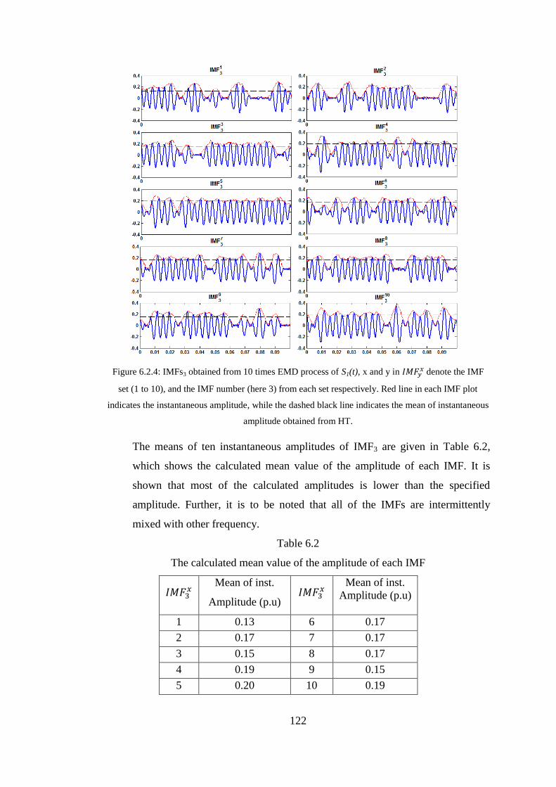
122
Figure 6.2.4: IMFs3 obtained from 10 times EMD process of S1(t), x and y in denote the IMF
set (1 to 10), and the IMF number (here 3) from each set respectively. Red line in each IMF plot
indicates the instantaneous amplitude, while the dashed black line indicates the mean of instantaneous
amplitude obtained from HT.
The means of ten instantaneous amplitudes of IMF3 are given in Table 6.2,
which shows the calculated mean value of the amplitude of each IMF. It is
shown that most of the calculated amplitudes is lower than the specified
amplitude. Further, it is to be noted that all of the IMFs are intermittently
mixed with other frequency.
Table 6.2
The calculated mean value of the amplitude of each IMF
Mean of inst.
Amplitude (p.u)
Mean of inst.
Amplitude (p.u)
1 0.13 6 0.17
2 0.17 7 0.17
3 0.15 8 0.17
4 0.19 9 0.15
5 0.20 10 0.19

123
4. Average the (ensemble) of corresponding IMFs to obtain the final result.
The mean of the third IMF is shown in Figure 6.2.5(a) and its
corresponding instantaneous amplitude, frequency and phase waveforms
obtained from the Hilbert Transform are shown in Figure 6.2.5 (b)-(d)
Figure 6.2.5: The Hilbert Transform of the averaged IMFs3 shown in Figure
6.2.4 (a)The averaged IMFs3 (b) The instantaneous frequency (c) The
instantaneous amplitude (d) The instantaneous phase angle.
Figure 6.2.5(a) demonstrates how the averaging process of to
shown in Figure 6.2.4 has successfully reduced the noise mixing
intermittently in the IMF3 component as shown in Figure 6.2.3 and the mean of
the instantaneous frequency of the IMF3 becomes close to the expected value
(250Hz), the highest frequency of the signal. The intermittent noise mixing in
the IMFs3 has been cancelled out by the averaging process of 10 trials. The
noise has been captured in the first and second IMFs. The only part that
survives the averaging process of IMFs3 is the waveform of the actual 250Hz
component. Figure 6.2.5(b) shows that the instantaneous frequency is much
smoother and its mean is close to 250Hz.
However, since the mean of the instantaneous amplitude of to
are smaller than the specified amplitude of the 250 Hz component, the
averaging process of IMFs3 will also produce a mean of the instantaneous
amplitude which is smaller than the specified value of the 250 Hz component.
a)
b)
c)
d)
124
The final results of EEMD process applied to S1(t) by using the
standard deviation of the added noise of 0.2 and using 500 ensembles are
shown in Table 6.3.
Table 6.3
The result of EEMD process on S1(t)
IMF Amp
(p.u)
Freq
(Hz)
Phase
(deg)
1 0.019 3023 -7.19
2 0.011 1618 12.15
3 0.161 250 49.80
4 0.252 150 64.23
5 0.985 50 1.39
Table 6.3 shows the result from HT of the IMFs. IMF1 and IMF2 contain the
noise component of the signal, while IMF3 to IMF5 contain the harmonic and
fundamental components of the signal. Table 6.3 demonstrates that the EEMD
process has managed to solve the mixed frequency issues associated with EMD
(shown in Figure 6.2.3). All the frequency components and the phase angle of the
signal have been identified accurately. However, the detected amplitudes are less
than the specified value as given by (6-1) resulting in a difference (error).
Since the mean value of the instantaneous frequency is correctly calculated by
the EEMD, it is proposed to overcome the inaccuracy of the detected amplitude by
using an iterative technique which is referred to as the Iterative EEMD (IEEMD).
6.3. The Proposed Iterative EEMD (IEEMD)
Similar to the Iterative HHT process, in the Iterative EEMD, the calculation
process is repeated iteratively in order to decompose additional information that still
remains within the residue.
In order to obtain an accurate result of the decomposition process of noisy
signal, it is necessary to identify and separate the IMFs associated with noise from
the IMFs associated with actual components which should not be mixed with other
frequency. The IMFs obtained from the EEMD process which are not related to the
noise and not mixed with other frequency are referred to as significant IMFs which
will be subtracted from the signal.
Based on many simulations in the research, the identification of the IMFs
associated with noise can be performed by checking the mean value of the
125
instantaneous frequency of the IMF. For example, the noisy signal in (6-1) is
specified with highest frequency 250Hz. The IMF frequency which represents the
correct component of the signal must not be greater than 250 Hz. Therefore, the IMF
frequency greater than 250 Hz does not represent any signal component and it should
only come from the noise. Further, our experiments show that the mean value of the
IMF frequency related to the noise component is always greater than 1000 Hz.
The IMFs associated with actual components must not be mixed and can be
identified by checking the standard deviation of the instantaneous phase angle. A
smooth (less fluctuating, low standard deviation) instantaneous phase angle plot is
the result from smooth instantaneous frequency and smooth instantaneous amplitude
of the IMF which indicates that the IMF is not mixed. In contrary, a high standard
deviation of instantaneous phase angle is an indication of mixed IMF which should
be considered as insignificant result of the process. Based on the experimental
results, the IMFs associated with actual components usually have standard deviations
of the instantaneous phase angle below 30.
In addition, the experimental results show that a small amplitude IMF may
produce erroneous phase angle calculation. Further, small amplitude also means that
it is not large enough to be considered as significant result of the process, therefore it
should be ignored. Based on the experiments, the criterion of choosing significant
IMF with max amplitude ≥ 2 % peak amplitude of S(t) works effectively to obtain
accurate results.
To identify the correct IMFs which represent the actual signal components, a
significance check is performed in the process, as shown in step 4 of the Iterative
EEMD algorithm.
The steps to apply the Iterative EEMD on a signal S(t) are as follows:
1. Carry out the steps in EEMD
2. Calculate the amplitude and frequency of IMF1 to IMFn by using HT and
choose all the significant IMFs. The significant IMFs must satisfy the
following conditions :
* Fundamental freq ≤ IMF freq ≤ noise freq (1000Hz) AND
* Max amplitude of (IMF) ≥ 2% peak amplitude of S(t)
AND
* The standard deviation of the instantaneous phase angle is below 30.

126
3. Assume the significant kth
IMF Pk(t)can be approximated by a sinusoidal
representation:
Pk(t) = sin(2π t + ) (6-6)
Where:
Pk(t) = sinusoidal representation of the IMF
= approximated amplitude of kth
IMF
= approximated frequency of kth
IMF
= approximated phase angle of k
th IMF
4. Subtract the approximation for the dominant components of the significant
IMFs from the original signal to obtain the residue, rk(t)
rk(t) = S(t) – Pk(t) (6-7)
Steps 1-4 are repeated on rk(t) until the amplitude of the significant IMFs
reaches a low threshold value, which is defined here as 3% of the maximum
amplitude of S(t) OR until no more significant IMF obtained by the
decomposition process.
5. As in the iterative HHT [47], it is possible that similar frequencies are
obtained during the iterative process of decomposition. For each frequency
, obtained in the iterative EEMD process, the sinusoidal representations
associated with that frequency can be added together as given in (6-8) and
then the Hilbert Transform is applied to obtain the amplitude, frequency and
phase of that frequency component. These sinusoids are then sorted by
frequency.
Rk = sin(2π t + ) + sin(2π t +
)+.......
..... sin(2π t +
) (6-8)
6.4. Results from the Iterative EEMD
As an example of applying EEMD iteratively to the simulated signal, consider
the result of the standard EEMD process shown in Table 6.3 as the result of first
iteration. The significant IMFs should then be chosen according to step 2. Since
IMF1 and IMF2 have mean frequencies more than 1000Hz, according to step 2 they
are not considered as significant. Further, IMF3, IMF4 and IMF5 have mean
frequencies that lie between fundamental frequency and 1000Hz. The mean
amplitudes are also greater than 2% of the peak amplitude of S(t) and the IMFs are
127
not mixed with other frequencies. Therefore, IMF3, IMF4 and IMF5 are chosen as the
significant IMFs which are then represented as sinusoidal waveforms with mean
amplitudes, mean frequencies and mean phases obtained from HT, according to step
3.
The proposed method of successively subtracting sinusoid representations of
the significant IMFs instead of the actual IMFs (which is the approach in the
standard EEMD) has led to greater accuracy when dealing with the simulated noisy
signal, as shown in Table 6.4
Table 6.4
The detected components of noisy signal S1(t) using IEEMD
Step
No
Amp
(p.u)
Freq
(Hz)
Phase
(deg)
MSE
(%)
1
0.167 250 49.81
0.44 0.247 150 62.63
0.947 50 0.67
Step
No
Amp
(p.u)
Freq
(Hz)
Phase
(deg)
MSE
(%)
2
0.021 250 49.87
0.13 0.069 150 51.95
0.029 50 -9.37
Step
No
Amp
(p.u)
Freq
(Hz)
Phase
(deg)
MSE
(%)
3 0.019 50 -14.27 0.11
Table 6.4 shows that some of the sinusoids obtained have the same frequency
value. The sinusoids of the same frequency are then combined to obtain the final
result as shown in Table 6.5.
Table 6.5
The Final Result of IEEMD process on noisy signal S1(t)
Amp Freq phase
0.187 250 49.8
0.315 150 60.3
0.994 50 0.1
Table 6.5 shows the final result of IEEMD process which is more accurate than
the result from the standard EEMD process as shown in Table 6.3.

128
To test the performance of the proposed method, the Iterative EEMD as well as
the standard EEMD are used to decompose a couple of simulated noisy signals with
various harmonic frequency components. A total 500 ensemble member (nE) with
the standard deviation of the added noise (a) 0.3 is used for the EEMD and IEEMD
process. The accuracy of the decomposition processes are evaluated by checking the
difference of the reconstructed signal (which is obtained by combining all the
detected components) and the original signal by using a Mean Square Error criterion
(MSE). Mean Square Error (MSE) of a calculation measures the mean or average of
the squares of the "errors", which is the difference between the calculated value and
the actual value [61]. The smaller the MSE value, the more accurate the
decomposition results are. The result of the accuracy test of the decomposition
processes is shown in Table 6.6.
Table 6.6
The MSE of the decomposition results using IEEMD and EEMD
Table 6.6 shows that for the simulated PQ harmonic signals used in the test, the
MSEs of the reconstructed signal (which is obtained by combining all the detected
components) and the original signal using the IEEMD process are significantly
smaller than the associated MSEs of the EEMD process. The results demonstrate that
the accuracy of the proposed IEEMD method is higher than the standard EEMD
technique.
6.5. Chapter Summary
This chapter has described the Ensemble Empirical Mode Decomposition
(EEMD) to resolve the mode mixing issues with the EMD. The EEMD has been
tested with noisy signals which usually produce mixed IMF when processed by using
EMD. The EEMD has been found to be effective in resolving the mode mixing
issues of the noisy signals. However, the identified amplitudes of the detected
components are found to be inaccurate. To resolve this problem, an iterative techique
which is referred to as the Iterative EEMD is proposed. The evaluation of the
MSE (%)
signal (Hz) EEMD IEEMD
50-250-450 0.672 0.123
50-350-650 0.268 0.133
50-450-850 0.502 0.162

129
proposed Iterative EEMD method to decompose various PQ signals has
demonstrated its accuracy over the standard EEMD.
130
CHAPTER 7 RESULTS
7.1. Introduction
This chapter will provide the decomposition results of measured signals by
using HHT, Iterative HHT, EEMD and the Iterative EEMD. The measured signals
are obtained from measurement at an industrial site using Dranetz PQ analyzer and
also from PQube cloud storage of PQ events.
First, the standard HHT will be used to decompose the measured signals.
Because of the noise content of the measured signals, mixed frequency IMFs will be
obtained, which may cause the decomposition process to miss one or more frequency
components. The Iterative HHT can decompose the measured signal more accurately
than the standard HHT, if the noise content is not too high. However, for more noisy
measured signals, the Iterative HHT will also miss one or more frequency
components due to mode mixing issue. To overcome this, the EEMD is used to
improve the decomposition process by resolving the problems of mixed IMFs. The
result of EEMD process of measured signals are found to be more accurate than the
Iterative HHT since the mixed IMFs issue are reduced significantly. However, as
discussed in the previous chapter, the amplitudes of the identified components by
EEMD process are usually smaller than the actual amplitudes. To produce more
accurate amplitudes of the decomposed components, the iterative EEMD is then
applied. Results from the decomposition process show that the noisy signals from the
Dranview measurement and Pqube data can be decomposed correctly using this
approach.
To decompose non-stationary signals, SAX method can be utilized to obtain
the instant of changes of the signal which are then used to segment the original signal
to a sequence of stationary signals. The iterative HHT or the iterative EEMD can
then be used to analyse each segment separately.
7.2. Measured Signals
7.2.1. Dranview Signal
The Dranview signal is obtained from a measurement of the 66kV phase „a‟
current at a point of common coupling to a plastic manufacturing facility in
Australia, using a Dranetz PQ monitoring instrument, Power Xplorer PX5. The
company produces small plastic pellets which are then used by other manufacturers
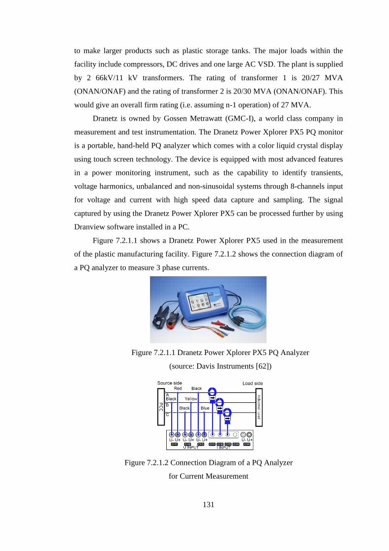
131
to make larger products such as plastic storage tanks. The major loads within the
facility include compressors, DC drives and one large AC VSD. The plant is supplied
by 2 66kV/11 kV transformers. The rating of transformer 1 is 20/27 MVA
(ONAN/ONAF) and the rating of transformer 2 is 20/30 MVA (ONAN/ONAF). This
would give an overall firm rating (i.e. assuming n-1 operation) of 27 MVA.
Dranetz is owned by Gossen Metrawatt (GMC-I), a world class company in
measurement and test instrumentation. The Dranetz Power Xplorer PX5 PQ monitor
is a portable, hand-held PQ analyzer which comes with a color liquid crystal display
using touch screen technology. The device is equipped with most advanced features
in a power monitoring instrument, such as the capability to identify transients,
voltage harmonics, unbalanced and non-sinusoidal systems through 8-channels input
for voltage and current with high speed data capture and sampling. The signal
captured by using the Dranetz Power Xplorer PX5 can be processed further by using
Dranview software installed in a PC.
Figure 7.2.1.1 shows a Dranetz Power Xplorer PX5 used in the measurement
of the plastic manufacturing facility. Figure 7.2.1.2 shows the connection diagram of
a PQ analyzer to measure 3 phase currents.
Figure 7.2.1.1 Dranetz Power Xplorer PX5 PQ Analyzer
(source: Davis Instruments [62])
Figure 7.2.1.2 Connection Diagram of a PQ Analyzer
for Current Measurement

132
The phase „a‟ current signals captured with sampling frequency 256 / 0.02 Hz
at various time from 7th
to 9th
of August 2012 are shown in Figures 7.2.1.3 (a-d),
which can be seen that sometimes the signal has very little noise content as shown by
the zoomed box in Figure 7.2.1.3(a) and (d). However, at other times the signals are
quite noisy as shown by the zoomed boxes in Figures 7.2.1.3 (b)-(c). Table 7.1
details the time when the signal data are recorded.
The noise content in the signal can be due to the starting of large motors at
some time during the day which can generate short term noise as well as possible
electromagnetic interference from starting power electronics equipment nearby.
Figure 7.2.1.3 The measured signals at various measurement time
a). Dranview#062, b). Dranview#214, c). Dranview#265, d). Dranview#427
7.2.2. PQube Signal
The PQube PQ analyzer produced by Power Standards Lab is a tiny, user-
friendly PQ recorder with built-in power and energy monitoring. All recorded data is
written directly onto an SD memory card installed in the device in a number of
ready-to-use formats and therefore, PQube doesn‟t require any specific software to
read the data. In addition, the recorded data can be sent to a cloud database of PQ
events.
a) b)
d) c)

133
Table 7.1
The Measurement time of Various Dranview Signals
Event name Measurement time
date time
Event#024 7/08/2012 4:20:00 PM
Event#037 7/08/2012 5:50:00 PM
Event#052 7/08/2012 8:20:00 PM
Event#062 7/08/2012 10:10:00 PM
Event#214 8/08/2012 2:10:00 PM
Event#265 8/08/2012 10:40:00 PM
Event#273 9/08/2012 12:00:00 AM
Event#298 9/08/2012 3:50:00 AM
Event#387 9/08/2012 4:20:00 PM
Event#427 9/08/2012 10:40:00 PM
The instruments have been used in many countries to record and share PQ data
for academic research. The recorded PQ data are regularly updated and available at
http://map.pqube.com which can be accessed as free public sources of information
[63]. Figure 7.2.2.1 shows PQube DRK-270-00, a variant of PQube power quality
analyzer devices.
Figure 7.2.2.1 PQube DRK-270-00 PQ analyzer device
(source: jsdata [64])
A voltage signal recorded at 20 July 2014 by a Pqube PQ measuring device
from single phase voltage measurement at Gossen Mettrawat (GMC-I) company in
Massy Cedex, France is shown in Figure 7.2.2.2(a). Figure 7.2.2.2(b) shows a current
signal recorded at 9 February 2011 by a Pqube device from phase „a‟ of a 3 phase
current measurement at IMH Technologies in UK. IMH Technologies LTD is a PQ
instrumentation consultant in Rochford, United Kingdom that has carried out

134
consultancy for major utilites and customers in United Kingdom and offshore to
solve PQ problems.
Figure 7.2.2.2 Pqube signal a) GMC-I signal, b) IMH signal
As shown in Figure 7.2.2.2(a), the noise content in the signal is less than the
other Pqube signal in Figure 7.2.2.2(b). Figure 7.2.2.2(b) shows a more noisy signal
as indicated by the multiple peaks at the top of the signal and also as shown in the
zoomed box. It will be demonstrated later that such signal will create problems for
the traditional decomposition techniques.
7.3. The analysis of the stationary measured signals.
In this section the less noisy PQ signal Dranview Event#062 shown in Figure
7.2.1.3(a) will be analysed by using the standard HHT. The iterative HHT is then
applied to improve the accuracy of the decomposition result. Another signal
Dranview Event#214 which is more noisy will then be used to demonstrate how the
standard HHT produces the intermittent mixed IMF from the decomposition process
in which the Iterative HHT is not able to resolve. The EEMD and Iterative EEMD is
then used to demonstrate the ability of the method to resolve the mode mixing issue
in the decomposition process of more noisy signal Dranview Event#214. A noisy
signal from the Pqube cloud storage is then used to further test the performance of
the decomposition methods to identify the components of the signal.
7.3.1. Dranview Signals
The phase „a‟ current signal (Dranview Event#062) measured by Dranetz
PowerXplorer PX5 shown in Figure 7.2.1.3(a) in Section 7.2.1 is first analyzed using
the standard HHT. The signal is first decomposed into IMFs using the EMD method.
Figure 7.3.1.1 shows the IMFs obtained from the EMD process.
a) b)

135
Figure 7.3.1.1 The IMFs obtained from the EMD process of Dranview Event#062
Figure 7.3.1.1 shows that the EMD process has decomposed the noise content
in IMF1 and IMF2. In IMF2, the noise is mixed with a small portion of the lower
frequency component which should be contained in IMF3. Therefore, the associated
portion of IMF3 waveform is lower due to the mixing issue.
When the IMFs are passed through the Hilbert Transform, the results are
shown in Table 7.2 which shows that the mean frequency of IMF1 and IMF2 are
around 4632 and 2711 Hz respectively, suggesting that IMF1 and IMF2 are related to
noise frequency. However the mean frequency of IMF3 is exactly 350 Hz which is
related to the 7th
harmonic of the 50Hz fundamental frequency signal in Australia.
Therefore, it can be concluded that the identified mean value of the instantaneous
frequency of IMF3 is quite accurate, which is 350 Hz. Table 7.2 suggesting that the
signal only contains the 50 Hz signal and the 7th harmonics. Figure 7.3.1.2 shows the
reconstructed signal from the identified 50Hz and 350Hz components compared with
the original signal. The residue (the difference between the reconstructed signal and
the original signal) is also shown in Figure 7.3.1.2. It can be observed that the
reconstructed signal is quite close to the measured signal. However, the residue of
the decomposition process indicates that some components of the signal are not
identified since the component was mixed with the high frequency (noise) content in
IMF2. Therefore, the iterative HHT should be used to obtain a better decomposition
result.
a)
b)
c)
d)
e)

136
Table 7.2
The Hilbert Transform results of IMFs
from EMD process of Dranview Event#062
IMF Amp
(p.u)
Freq
(Hz)
Phase
(deg)
1 0.118 4632 -0.51
2 0.076 2711 0.60
3 4.417 350 -114.80
4 59.528 50 80.99
Figure 7.3.1.2 Final result of HHT process of Dranview Event#062; the original
signal, the reconstructed signal and the residue
To obtain more accurate decomposition result of the measured signals using
the Iterative HHT process, a modification of the algorithm is necessary since the first
IMF from the EMD process of the measured signal always related to the noise
content which should be disregarded as part of the signal components. Therefore, a
technique to identify the significant IMFs which will be processed further (similar to
the Iterative EEMD algorithm described in section 6.3) is also used by the Iterative
HHT to process the measured signals. The sinusoidal representations of all the
significant IMFs (not from the first significant IMF only) are then subtracted from
the signal being analyzed.
By applying the modified Iterative HHT algorithm, the high frequency IMF1
and IMF2 shown in Table 7.2 are considered insignificant and will be ignored since
they are related to the noise content. The sinusoidal representations of IMF3 and
e)
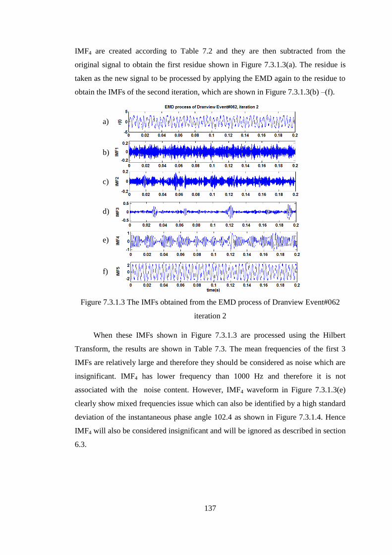
137
IMF4 are created according to Table 7.2 and they are then subtracted from the
original signal to obtain the first residue shown in Figure 7.3.1.3(a). The residue is
taken as the new signal to be processed by applying the EMD again to the residue to
obtain the IMFs of the second iteration, which are shown in Figure 7.3.1.3(b) –(f).
Figure 7.3.1.3 The IMFs obtained from the EMD process of Dranview Event#062
iteration 2
When these IMFs shown in Figure 7.3.1.3 are processed using the Hilbert
Transform, the results are shown in Table 7.3. The mean frequencies of the first 3
IMFs are relatively large and therefore they should be considered as noise which are
insignificant. IMF4 has lower frequency than 1000 Hz and therefore it is not
associated with the noise content. However, IMF4 waveform in Figure 7.3.1.3(e)
clearly show mixed frequencies issue which can also be identified by a high standard
deviation of the instantaneous phase angle 102.4 as shown in Figure 7.3.1.4. Hence
IMF4 will also be considered insignificant and will be ignored as described in section
6.3.
a)
b)
c)
d)
e)
f)

138
Table 7.3
The HT results of IMFs from IHHT process
of Dranview Event#062 iteration 2
IMF Amp
(p.u) Freq
(Hz) Phase
(deg)
1 0.119 4612 -1.71
2 0.075 2719 2.41
3 0.079 1643 7.5
4 0.447 660 6.59
5 2.436 250 143.81
Figure 7.3.1.4 The HT of IMF4 shown in Figure 7.3.1.3(e)
As shown in Table 7.3, the only signal that can be obtained from the second
iteration is the additional 250Hz component obtained from IMF5. The sinusoid
representation of IMF5 is then created and subtracted from the signal being analyzed
to obtain the next residue. When the residue is processed, there is no more significant
frequency component obtained and therefore the process is terminated. The
reconstructed signal built from the detected components of 50Hz, 250Hz and 350 Hz
given in Table 7.2 and Table 7.3 is shown in Figure 7.3.1.5(a) when compared to the
original signal.
Figure 7.3.1.5 shows that 3 sinusoidal representations of IMFs have been
detected by using the proposed Iterative HHT. There is no mixed IMF and the
reconstructed signal is quite close to the original. The Hilbert Transform of the final
result of the Iterative HHT process is shown in Table 7.4.
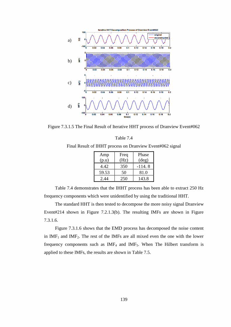
139
Figure 7.3.1.5 The Final Result of Iterative HHT process of Dranview Event#062
Table 7.4
Final Result of IHHT process on Dranview Event#062 signal
Amp
(p.u)
Freq
(Hz)
Phase
(deg)
4.42 350 -114. 8
59.53 50 81.0
2.44 250 143.8
Table 7.4 demonstrates that the IHHT process has been able to extract 250 Hz
frequency components which were unidentified by using the traditional HHT.
The standard HHT is then tested to decompose the more noisy signal Dranview
Event#214 shown in Figure 7.2.1.3(b). The resulting IMFs are shown in Figure
7.3.1.6.
Figure 7.3.1.6 shows that the EMD process has decomposed the noise content
in IMF1 and IMF2. The rest of the IMFs are all mixed even the one with the lower
frequency components such as IMF4 and IMF5. When The Hilbert transform is
applied to these IMFs, the results are shown in Table 7.5.
a)
b)
c)
d)

140
Figure 7.3.1.6 The result of EMD on Dranview#214
Table 7.5
The HT of the IMFs from EMD process on Dranview#214
IMF Amp
(p.u)
Freq
(Hz)
Phase
(deg)
1 0.52 4191 -0.29
2 0.34 2130 8.72
3 3.72 480 3.36
4 38.96 108 4.67
5 26.92 39 -38.91
Table 7.5 shows that no multiple of 50Hz frequecy is obtained from all the
IMFs suggesting the failure of the decomposition process using the standard HHT
when analysing more noisy signal such as Dranview Event#214.
The instantaneous frequency, amplitude and phase of IMF3, IMF4 and IMF5
obtained from the Hilbert Transform are shown in Figure 7.3.1.7.
The standard deviation of the the instantaneous phase angle of IMF3, IMF4 and
IMF5 also indicate that the IMFs are mixed as shown in Figure 7.3.1.7. The mixing
issue causes the calculated mean value of instantaneous frequencies are incorrect and
therefore, applying the Iterative HHT for this case will not help to obtain more
accurate result.
a)
b)
c)
d)
e)
f)
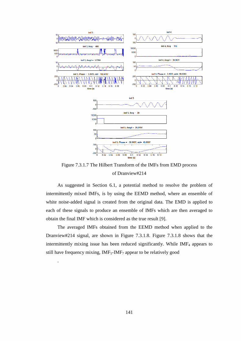
141
Figure 7.3.1.7 The Hilbert Transform of the IMFs from EMD process
of Dranview#214
As suggested in Section 6.1, a potential method to resolve the problem of
intermittently mixed IMFs, is by using the EEMD method, where an ensemble of
white noise-added signal is created from the original data. The EMD is applied to
each of these signals to produce an ensemble of IMFs which are then averaged to
obtain the final IMF which is considered as the true result [9].
The averaged IMFs obtained from the EEMD method when applied to the
Dranview#214 signal, are shown in Figure 7.3.1.8. Figure 7.3.1.8 shows that the
intermittently mixing issue has been reduced significantly. While IMF4 appears to
still have frequency mixing, IMF5-IMF7 appear to be relatively good
.

142
Figure 7.3.1.8 The resulting IMFs from the EEMD process of Dranview#214 signal.
Figure 7.3.1.8 demonstrates that the averaging process of the ensemble of IMFs
has recovered the IMFs from the mixing issue. The Hilbert Transform is then applied
to these averaged IMFs and the results are shown in Table 7.6.
Table 7.6
The HT of the IMFs from the EEMD process
of Dranview#214 signal.
IMF Amp
(p.u)
Freq
(Hz)
Phase
(deg)
1 0.427 4101 -0.38
2 0.183 2675 2.75
3 0.148 1640 1.18
4 1.644 355 -0.78
5 2.764 350 -76.13
6 54.328 50 86.71
7 0.634 50 118.39
MSE = 6.5948%
Table 7.6 shows that three components are identified, 350 Hz, 50 and 50 Hz.
The instantaneous frequency, amplitude and phase of IMF5, IMF6 and IMF7 obtained
from the Hilbert Transform are shown in Figure 7.3.1.9.
a)
b)
c)
d)
e)
f)
g)
h)

143
Figure 7.3.1.9 The Hilbert Transform of the IMFs from EEMD process of
Dranview#214
Figure 7.3.1.9 shows that the standard deviation of the instantaneous phase
angle of IMF5, IMF6 and IMF7 are quite low which indicate that the IMFs are not
mixed. The results demonstrate the superiority of the EEMD process to resolve the
intermittently mixed IMF issue.
However, the calculated MSE (Mean Square Error) between the reconstructed
signal and the original signal 6.59% is relatively high, suggesting that there are still
part of the signal that have not been identified from the decomposition process using
EEMD, therefore, as discussed in Section 6.2, the proposed Iterative EEMD needs to
be applied to the signal to obtain a better decomposition result. For the iterative
EEMD method, the result in Table 7.6 is considered as the outcome of the first
iteration and then more iterations will be applied to the residue of the first iteration.
The iteration process is applied until the stopping criterion is met, i.e the
amplitude of the significant IMFs reaches a low threshold value (3% of the
maximum amplitude of the original signal) or no more significant IMF is obtained.
The result of the IEEMD process is shown in Table 7.7.

144
Table 7.7
The HT of the IMFs from IEEMD process of Dranview#214
Amp
(p.u)
Freq
(Hz)
Phase
(deg)
2.764 350 -76.13
54.328 50 86.71
0.634 50 118.39
1.343 250 28.15
1.167 350 -108.60
Table 7.7 shows that 2 more components are identified in the next iterations.
The components with similar frequencies are then accumulated to obtain the final
result. Table 7.8 shows the final result of the IEEMD process.
Table 7.8
Final Result of IEEMD process of Dranview#214
Amp
(p.u) Freq
(Hz) Phase
(deg)
3.916 350 -165.12
1.343 250 -61.86
54.952 50 -3.34
Table 7.8 shows that more accurate result is obtained. The MSE between the
constructed signal and the original signal is 2.21%., which is within the accepted
tolerance and therefore the iteration is terminated.
Figure 7.3.1.10 shows the final result of IEEMD process of
DranviewEvent#214.
Figure 7.3.1.10 Final result of IEEMD process of DranviewEvent#214
a)
b)
c)
d)

145
Figure 7.3.1.10 shows that the sinusoidal representations of the IMFs do not
have any mixing issue, in addition the calculated MSE between the reconstructed
signal shown in Figure 7.3.1.10 (a) and the original signal 2.21% is more accurate
than the result of the standard EEMD with the MSE 6.59%.
7.3.2. PQube Signal
The phase „a‟ measured current signal from Pqube cloud storage shown in
Figure 7.2.2.2 is first analysed using the standard HHT. The signal is decomposed by
using the EMD process to obtain the IMFs as shown in Figure 7.3.2.1.
Figure 7.3.2.1 The IMFs obtained from EMD process of Pqube signal
Figure 7.3.2.1 shows that the EMD process has extracted the noise content in
IMF1 and IMF2. In IMF2, the noise is intermittently mixed with lower frequency
component. Similarly, IMF3 and IMF4 appear to also be mixed with another lower
frequency components, while IMF5 is the only IMF which does not look mixed.
When the Hilbert Transform is applied to the IMFs to obtain the intantaneous
amplitude, frequency and phase waveforms, the results are shown in Table 7.9.
Table 7.9 shows that the mean frequency of IMF1 and IMF2 are 2154 Hz and
1267 Hz respectively, suggesting that IMF1 and IMF2 are related to noise frequency.
The frequency of the rest of the IMFs are lower than a typical noise frequency (1000
Hz), however it is necessary to check which IMF is significant by evaluating the
standard deviation of the instantaneous phase angle of the IMFs.
a)
b)
c)
d)
e)
f)

146
Table 7.9
The HT of the IMFs from EMD process of Pqube signal
IMF Amp
(p.u)
Freq
(Hz)
Phase
(deg)
1 0.29 2154 -11.00
2 0.26 1267 0.93
3 0.92 540 5.21
4 1.62 280 1.73
5 23.02 50 -148.29
To identify which IMF is mixed, the instantaneous phase angles of the IMFs
obtained from the Hilbert Transform are processed to identify their standard
deviations. The standard deviation of the instantaneous phase angle of the IMFs are
shown in Figure 7.3.2.2.
Figure 7.3.2.2 The Hilbert Transform of the IMFs from EMD process
of Pqube signal
Figure 7.3.2.2 shows that the mean frequency of IMF3 is 540 Hz which is
lower then a typical noise frequency (1000 Hz), however, it is mixed with other
frequency which is indicated by the unstability of the instantaneous phase angle with
very high standard deviation around 101 and therefore the IMF can not be used as a

147
correct representation of the signal component. Similarly, the standard deviation of
instantaneous phase angle plot of IMF4 is 110 which is higher than the threshold,
indicating that it is mixed with other frequency and therefore, the result can be
considered erroneous. The only non-mixed IMF obtained by the standard HHT is
IMF5 which is the fundamental frequency component in the UK, 50 Hz. Since most
of the IMFs obtained are mixed, the result of the decomposition process using the
standard HHT is inaccurate which is indicated by the calculated MSE between the
reconstructed signal and the original signal equals 22.22%.
To obtain more accurate result, the Iterative HHT process is then used to
decompose the signal. In the Iterative HHT process, IMF1 and IMF2 shown in Table
7.9 are considered insignificant since they are related with noise. IMF3 and IMF4 are
also considered as insignificant since they are mixed with other frequencies. IMF5 is
the only significant IMF which is processed further by creating its sinusoidal
representation according to Table 7.9. The sinusoidal representation is then
subtracted from the signal to obtain the first residue. The EMD process is again
applied to the residue to obtain the IMFs as shown in Figure 7.3.2.3.
Figure 7.3.2.3 The IMFs obtained from EMD process of Pqube signal Iteration 2
The mean value of the instantaneous frequency, amplitude and phase obtained
from the Hilbert Transform of the IMFs is shown in Table 7.10.
a)
b)
c)
d)
e)
f)
g)
h)

148
Table 7.10
The Hilbert Transform of IMFs
from IHHT process of Pqube signal iteration 2
IMF Amp
(p.u) Freq
(Hz) Phase
(deg) IMF
Amp
(p.u)
Freq
(Hz)
Phase
(deg)
1 0.30 2104 3.39 5 1.57 120 32.46
2 0.34 1093 15.87 6 0.54 80 37.20
3 1.24 430 3.57 7 0.20 50 -74.52
4 2.28 200 10.67
Table 7.10 indicates that IMF1 and IMF2 are related to the noise frequency,
while the rest of IMFs are lower than the noise frequency. To identify which IMF is
mixed, the Hilbert Transform is used to calculate the instantaneous frequency,
amplitude and phase of IMF3, IMF4 and IMF5. The standard deviation of the
instantaneous phase angle of the IMFs are then calculated as shown in Figure 7.3.2.4.
Figure 7.3.2.4 The Hilbert Transform of IMF3, IMF4, IMF5, IMF6 and IMF7 from
Iterative HHT process of Pqube signal at iteration 2
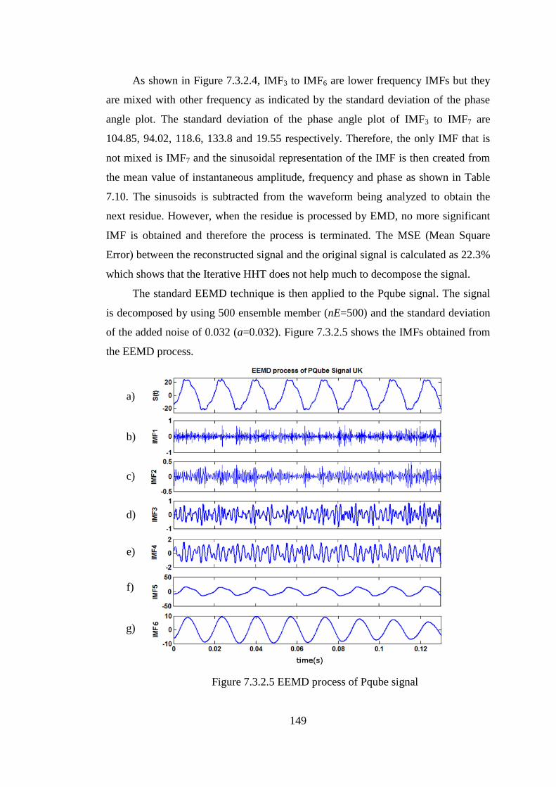
149
As shown in Figure 7.3.2.4, IMF3 to IMF6 are lower frequency IMFs but they
are mixed with other frequency as indicated by the standard deviation of the phase
angle plot. The standard deviation of the phase angle plot of IMF3 to IMF7 are
104.85, 94.02, 118.6, 133.8 and 19.55 respectively. Therefore, the only IMF that is
not mixed is IMF7 and the sinusoidal representation of the IMF is then created from
the mean value of instantaneous amplitude, frequency and phase as shown in Table
7.10. The sinusoids is subtracted from the waveform being analyzed to obtain the
next residue. However, when the residue is processed by EMD, no more significant
IMF is obtained and therefore the process is terminated. The MSE (Mean Square
Error) between the reconstructed signal and the original signal is calculated as 22.3%
which shows that the Iterative HHT does not help much to decompose the signal.
The standard EEMD technique is then applied to the Pqube signal. The signal
is decomposed by using 500 ensemble member (nE=500) and the standard deviation
of the added noise of 0.032 (a=0.032). Figure 7.3.2.5 shows the IMFs obtained from
the EEMD process.
Figure 7.3.2.5 EEMD process of Pqube signal
a)
b)
c)
d)
e)
f)
g)

150
Figure 7.3.2.5 shows the IMFs obtained from the EEMD process of Pqube
signal. The EEMD process has extracted the noise content in IMF1 and IMF2. IMF3
to IMF6 show less mixed frequency waveforms. It is obvious that the averaging
process of the ensemble of IMFs has reduced the mode mixing issues that appeared
in the result of HHT process shown in Figure 7.3.2.1. The mean value of the
instantaneous frequency, amplitude and phase obtained from the Hilbert Transform
of the IMFs is shown in Table 7.11.
Table 7.11
The HT of IMFs from EEMD process of Pqube signal
IMF Amp
(p.u) Freq
(Hz) Phase
(deg) IMF
Amp
(p.u)
Freq
(Hz)
Phase
(deg)
1 0.242 2539 -3.19 4 1.047 360 -1.405
2 0.145 1450 -6.65 5 13.838 50 -147.455
3 0.437 510 0.455 6 8.905 50 -149.406
Table 7.11 shows that the mean value of instantaneous frequency of IMF1 and
IMF2 are greater than 1000 Hz which indicates that they are related to the noise
content of the signal. While the mean value of instantaneous frequency of IMF3 to
IMF6 are lower than 1000 Hz. To identify which IMF is mixed, the standard
deviation of the instantaneous phase angle obtained from HT of the IMFs are then
calculated as shown in Figure 7.3.2.6.
Figure 7.3.2.6 The Hilbert Transform of the IMFs in Figure 7.3.2.5
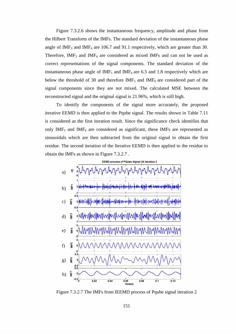
151
Figure 7.3.2.6 shows the instantaneous frequency, amplitude and phase from
the Hilbert Transform of the IMFs. The standard deviation of the instantaneous phase
angle of IMF3 and IMF4 are 106.7 and 91.1 respectively, which are greater than 30.
Therefore, IMF3 and IMF4 are considered as mixed IMFs and can not be used as
correct representations of the signal components. The standard deviation of the
instantaneous phase angle of IMF5 and IMF6 are 6.5 and 1.8 respectively which are
below the threshold of 30 and therefore IMF5 and IMF6 are considered part of the
signal components since they are not mixed. The calculated MSE between the
reconstructed signal and the original signal is 21.96%, which is still high.
To identify the components of the signal more accurately, the proposed
iterative EEMD is then applied to the Pqube signal. The results shown in Table 7.11
is considered as the first iteration result. Since the significance check identifies that
only IMF5 and IMF6 are considered as significant, these IMFs are represented as
sinusoidals which are then subtracted from the original signal to obtain the first
residue. The second iteration of the Iterative EEMD is then applied to the residue to
obtain the IMFs as shown in Figure 7.3.2.7 .
Figure 7.3.2.7 The IMFs from IEEMD process of Pqube signal iteration 2
a)
b)
c)
d)
e)
f)
g)
h)

152
Figure 7.3.2.7 shows the IMFs obtained from iteration 2 of the EEMD process
of Pqube signal. The mean value of the Hilbert Transform of the IMFs are shown in
Table 7.12.
Table 7.12
The HT of the IMFs in Figure 7.3.2.7
IMF Amp
(p.u) Freq
(Hz) Phase
(deg)
1 0.243 2098 -2.87
2 0.147 1215 -9.86
3 0.424 530 -6.44
4 1.061 400 -5.88
5 2.219 150 9.94
6 0.238 260 -3.89
7 0.172 50 -147.04
8 0.098 50 -76.55
Table 7.12 shows that the EEMD process has extracted the noise content in
IMF1 and IMF2. While the mean value of instantaneous frequency of IMF3 to IMF7
are lower than noise frequency. To identify which IMF is mixed, the Hilbert
Transform is used to calculate the instantaneous frequency, amplitude and phase of
IMF3 to IMF8. The standard deviation of the instantaneous phase angle the IMFs are
then calculated as shown in Figure 7.3.2.8.
Figure 7.3.2.8 shows that the mean frequency of IMF3 to IMF8 are lower then a
typical noise frequency (1000 Hz). However, IMF3, IMF4, IMF6 and IMF8 are mixed
with other frequency which are indicated by the unstability of the instantaneous
phase angle with standard deviation greater than 30 and therefore the IMFs can not
be considered as the significant results of the process. The standard deviation of the
instantaneous phase angle of IMF5 and IMF7 are 16.178 and 8.49 respectively and
therefore they are considered as significant IMFs and will be processed further. The
sinusoidal representation of these IMFs are then created and subtracted from the
waveform being analyzed to obtain the second residue. The calculated MSE between
the cumulative identified components to the original signal is 8.84%.
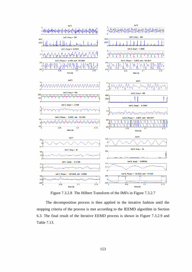
153
Figure 7.3.2.8 The Hilbert Transform of the IMFs in Figure 7.3.2.7
The decomposition process is then applied in the iterative fashion until the
stopping criteria of the process is met according to the IEEMD algorithm in Section
6.3. The final result of the Iterative EEMD process is shown in Figure 7.3.2.9 and
Table 7.13.

154
Figure 7.3.2.9 The Final result of Iterative EEMD process of Pqube signal
Table 7.13.
The result of the HT of the IMFs from Pqube signal
Amp
(p.u) Freq
(Hz) Phase
(deg)
13.838 50 -147.45
8.905 50 -149.41
2.219 150 9.94
0.172 50 -147.04
0.546 250 -136.51
0.327 150 -0.44
0.118 50 7.10
0.832 350 -58.25
0.329 250 -130.92
0.053 50 25.61
Table 7.13 shows the result of the Iterative EEMD of the Pqube signal until 4
iterations (the next iteration does not give significant IMF any more and therefore the
process is terminated at iteration 4). The IMFs with similar frequency are then
combined to obtain the final result shown in Table 7.14.
Table 7.14.
The final result of the IEEMD process of Pqube signal
IMF Amp
(p.u) Freq
(Hz) Phase
(deg) IMF
Amp
(p.u)
Freq
(Hz)
Phase
(deg)
1 0.832 350 -58.25 3 2.541 150 8.61
2 0.873 250 -134.41 4 22.753 50 -148.07
a)
b)
c)
d)
e)
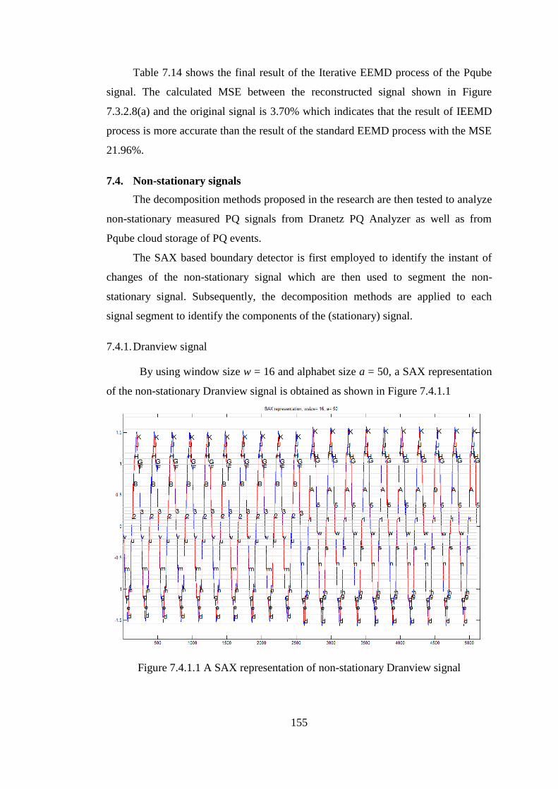
155
Table 7.14 shows the final result of the Iterative EEMD process of the Pqube
signal. The calculated MSE between the reconstructed signal shown in Figure
7.3.2.8(a) and the original signal is 3.70% which indicates that the result of IEEMD
process is more accurate than the result of the standard EEMD process with the MSE
21.96%.
7.4. Non-stationary signals
The decomposition methods proposed in the research are then tested to analyze
non-stationary measured PQ signals from Dranetz PQ Analyzer as well as from
Pqube cloud storage of PQ events.
The SAX based boundary detector is first employed to identify the instant of
changes of the non-stationary signal which are then used to segment the non-
stationary signal. Subsequently, the decomposition methods are applied to each
signal segment to identify the components of the (stationary) signal.
7.4.1. Dranview signal
By using window size w = 16 and alphabet size a = 50, a SAX representation
of the non-stationary Dranview signal is obtained as shown in Figure 7.4.1.1
Figure 7.4.1.1 A SAX representation of non-stationary Dranview signal

156
Figure 7.4.1.1 shows the symbolic representation of the non-stationary signal
which illustrates the repetitive patterns of the signal. It can be seen that the pattern in
the first 10 cycles are different to the pattern of the next cycles, which demonstrates
the ability of SAX algorithm to tanslate the original signal to a more simple
representation that can be used for a boundary identification process. The boundary
detector algorithm is then applied to the symbolic representation to identify instant of
changes as shown in Table 7.15
Table 7.15
The SAX word for two consecutive cycles of non-stationary Dranview signal
S1(n1) S2(n2) Euclidean
Dist Sum n1
symbol
l1 value n2
symbol
l2 value
157 'K' 47 141 'K' 47 0
158 'G' 43 142 'G' 43 0
159 'F' 42 143 'F' 42 0
160 '3' 30 144 '3' 30 0
161 'n' 14 145 'v' 22 8
As shown in Table 7.15, the instant of change is detected at point no 161 which
coincides with t = 0.2 sec. Using this point of change, the non-stationary signal is
then divided into 2 segments which are then analyzed using the decomposition
methods.
The decomposition of these 2 segments will be performed by the EEMD and
Iterative EEMD techniques since these methods have shown higher accuracy than the
standard HHT and Iterative HHT for measured signal decomposition. The result of
decomposition process using the standard EEMD and the Iterative EEMD are shown
in Table 7.16 and Table 7.17 respectively
Table 7.16
Result of EEMD decomposition of non-stationary Dranview signal
IMF
segment 1 segment 2
Amp (p.u)
Freq (Hz)
Phase (deg)
Amp (p.u)
Freq (Hz)
Phase (deg)
1 0.3 4263 1.01 0.32 4276 -1.06
2 0.15 2594 -8.92 0.15 2624 -2.09
3 0.12 1650 -8.39 0.12 1499 6.23
4 4.45 350 -134.04 5.05 350 -139.55
5 4.34 1250 -1.67 4.16 1385 0.74
6 44.83 50 87.46 46.8 50 85.41

157
Table 7.17
Result of IEEMD decomposition of non-stationary Dranview signal
IMF
segment 1 segment 2
Amp (p.u)
Freq (Hz)
Phase (deg)
Amp (p.u)
Freq (Hz)
Phase (deg)
1 4.45 350 135.95 5.33 350 130.44
2 0.27 150 -145.21 0.11 150 -135.28
3 49.16 50 85.8 51.2 50 83.7
Table 7.16 and Table 7.17 show the detected components of the non-stationary
signal using EEMD and IEEMD. The reconstructed signal is then created from the
detected components which is then compared to the original signal to estimate their
difference. The calculated MSE between the original signal and the reconstructed
signal using EEMD and IEEMD methods are 21.96% and 6.06% respectively which
demonstrates the accuracy of the IEEMD process over the standard EEMD method.
Figure 7.4.1.2 shows the final result of the Iterative EEMD process of the non-
stationary signal.
Figure 7.4.1.2 Final result of the Iterative EEMD process on non-stationary
Dranview signal
Figure 7.4.1.2 shows that the proposed Iterative EEMD has decomposed the
non-stationary Dranview signal accurately.

158
7.4.2. PQube signal
The proposed method is also applied to decompose a 3-phase signal available
from a UK voltage sag snapshot event from the PQube cloud storage of PQ events
[65], as shown in Figure 7.4.2.1. The occurrence of the event is 6.95 sec, the detected
voltage swell level is 173% with rated frequency 50 Hz and rated voltage 240 / 415
V.
Figure 7.4.2.1 The PQube voltage sag signal
The snapshot shows some missing point in the top plot representing some time
lapse during the transition. For the purposes of this study, the signal is assumed to be
continuous and connected as shown in Figure 7.4.2.2 (a). The SAX boundary
detector is then used to identify the boundaries of the signal as shown in Table 7.18.
Table 7.18 The detected boundaries of PQube signal
Segment 1 Segment 2 Segment 3 Segment 4
0 - 0.083 sec 0.0831 - 0.188 sec 0.01881 - 0.272 sec 0.2721 -0.3555 sec
The IEEMD using 500 ensemble member (nE=500) and the standard deviation
of the added noise 0.032 (a=0.032) is then applied to the signal, which produces the
results shown in Figures 7.4.2.2 (b) – (e). Two main frequencies were identified; 50
Hz and 150 Hz denoted as IMF1 and IMF2 in Figures 7.4.2.2(b) - (c). The residue of
the decomposition process is shown in Figure 7.4.2.2(d) which is relatively small
(around 4% of the original signal).
The three instantaneous phases in each segment of the 50 Hz three phase signal
are shown in Figure 7.4.2.2 (e) in a phasor form. It is interesting to note that the three
phases are, as expected, phase shifted by 120 degrees during normal operation in
segments 1 and 4, but when voltage sag occurs in phase „a‟ (60% in segment 2 and
1% in segment 3), the three phases are now unbalanced, with phase „b‟ and phase „c‟
being larger and the three phases are no longer phase shifted by 120 degrees as
shown in Figure 7.4.2.2 (e) for segments 2 and 3.
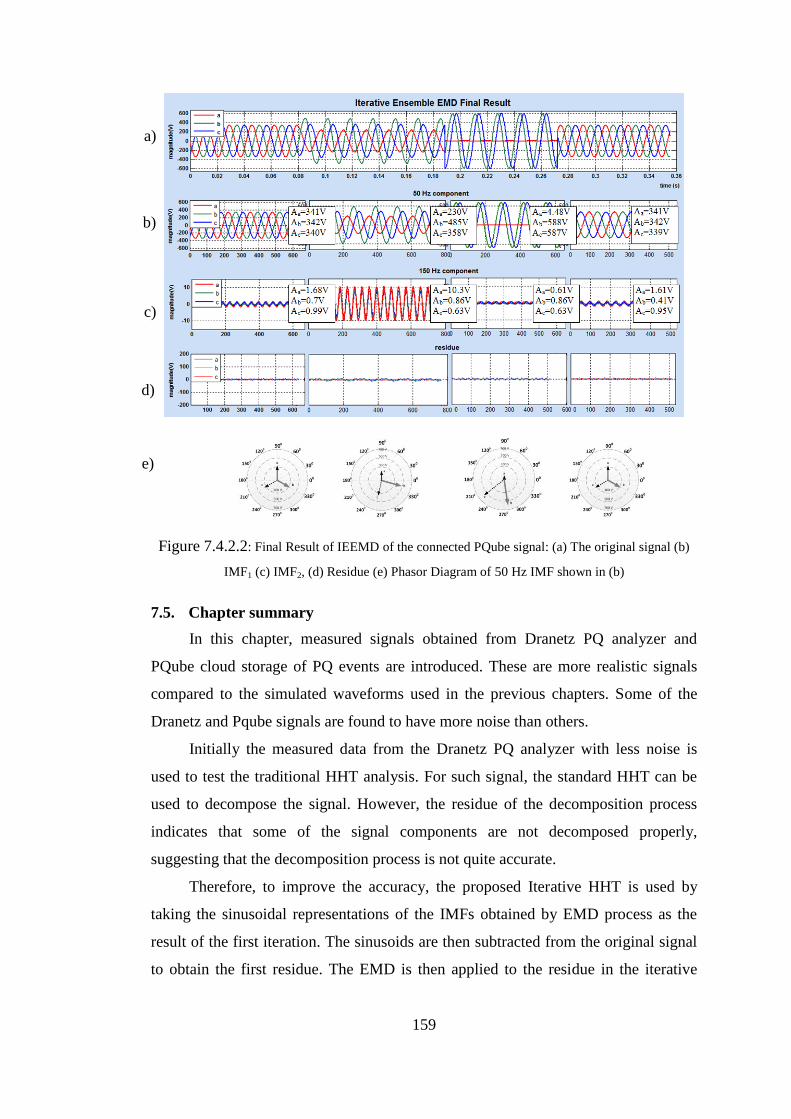
159
Figure 7.4.2.2: Final Result of IEEMD of the connected PQube signal: (a) The original signal (b)
IMF1 (c) IMF2, (d) Residue (e) Phasor Diagram of 50 Hz IMF shown in (b)
7.5. Chapter summary
In this chapter, measured signals obtained from Dranetz PQ analyzer and
PQube cloud storage of PQ events are introduced. These are more realistic signals
compared to the simulated waveforms used in the previous chapters. Some of the
Dranetz and Pqube signals are found to have more noise than others.
Initially the measured data from the Dranetz PQ analyzer with less noise is
used to test the traditional HHT analysis. For such signal, the standard HHT can be
used to decompose the signal. However, the residue of the decomposition process
indicates that some of the signal components are not decomposed properly,
suggesting that the decomposition process is not quite accurate.
Therefore, to improve the accuracy, the proposed Iterative HHT is used by
taking the sinusoidal representations of the IMFs obtained by EMD process as the
result of the first iteration. The sinusoids are then subtracted from the original signal
to obtain the first residue. The EMD is then applied to the residue in the iterative
e)
a)
b)
c)
d)

160
fashion. The result of the Iterative HHT is found to be more accurate than the
standard HHT method.
However, when the Dranetz waveform with a higher level of noise such as
Dranview#214 was used, the HHT produces intermittently mixed frequencies in the
IMFs which causes the Hilbert Transform to produce incorrect mean frequencies
calculation. Therefore, some frequency components are missed out resulting in
inaccurate decomposition.
When the Dranetz waveform is processed using the Iterative HHT, the first
IMF (after ignoring IMFs that appear as noise) also contains intermittently mixed
frequency, which causes the calculated mean of the instantaneous frequency from the
Hilbert Transform is inaccurate. Therefore, using sinusoidal representation of the
IMFs and subtracting them from the original signal will not help to identify actual
frequency components of the signal.
To resolve the problem, the standard EEMD technique is used where an
ensemble of white noise-added signals is created from the original data. The EMD is
applied to each of these signals to produce an ensemble of IMFs which are then
averaged to obtain the final IMF which is considered as the true result [9]. The
averaged IMFs obtained by EEMD is far less mixed than the IMFs obtained by EMD
process, and therefore, more accurate results of the mean value of the instantaneous
amplitudes, frequencies and phases of each decomposed component can be obtained
using the Hilbert Transform. However, as discussed in Chapter 6 and shown in the
calculation result of this chapter, EEMD process usually produce smaller values of
the mean amplitudes. When the MSE between the reconstructed signal and the
original signal is calculated, the value is still higher than the accepted tolerance
confirming this potential issue.
To improve the decomposition process, the proposed IEEMD is used to
decompose the signal components remaining in the residue. The result from the
Iterative EEMD is found to be more accurate than the standard EEMD and the
calculated MSE between the reconstructed signal and the original signal is now
within the accepted tolerance.
Finally, the non-stationary signals from Dranetz and Pqube are used to test the
decomposition method. As discussed in Chapter 3, while EMD method can obtain
automatically the instantaneous amplitude, frequency and phase in the non-stationary

161
signal, inaccuracies occur on the instantaneous amplitude, frequency and phase due
to overshoot and ambiguity around the area of a transition/discontinuity. Therefore,
the SAX based boundary detector is applied to the symbolic representation of the
signal, to identify the instants of changes in the non-stationary signal. After obtaining
the boundaries of the signal by using SAX algorithm, the signals are segmented
according to the identified boundaries and the decomposition methods are then
applied to each segment. The results show that the Iterative EEMD method can
decompose the signal more accurately than the standard EEMD.
This chapter shows that the developed methods in Chapter 4 to Chapter 6 can
provide accurate decompositions of both stationary and non stationary signals,
particularly with the help of the iterative EMD methods and the SAX-based
boundary detector.

162
CHAPTER 8 CONCLUSION
8.1. Discussions and Conclusions of the Research Work
This final chapter presents a summary of the thesis and the conclusion it draws.
The thesis presents the outcome of a Ph.D research program that focused on
investigating the effectiveness of the recently developed methods for decomposing
both stationary and non-stationary PQ signals such as Hilbert Huang Transform
(HHT) and the Ensemble Empirical Mode Decomposition (EEMD) technique, and
methods to improve their accuracy.
PQ issue has become a major concern since poor PQ can cause failure or
malfunction of sensitive electrical equipment. The electric utilities need to ensure
that they provide the customers with a good PQ level to obtain the customers
satisfaction. PQ monitoring and PQ troubleshooting are becoming more important to
the electric utilities to provide a high level of service.
In Chapter 2, the issue of PQ disturbances on power systems has been
discussed, followed by a discussion of their effects to the equipment. A PQ
disturbance classification based on the IEEE 1159-1995 and IEC 61000 classification
method shows that there are several PQ disturbances that need to be considered. To
help identify PQ problems, PQ meters are required. Many utilities are now
considering to carry out PQ monitoring study of their system and therefore more PQ
meters will be installed to monitor the PQ of their system. The analysis of the PQ
data collected by the instruments is needed to identify the type of PQ disturbance, in
particular the amount of harmonic components, swell, sags, flickers etc.
Several methods to decompose PQ waveforms into their components have also
been described. FFT is reported to have difficulties to analyze non - stationary signal,
and therefore STFT is developed to enable the FFT algorithm work for non-
stationary waveforms. However, STFT has a fixed resolution which depends on the
fixed window size which is chosen before the analysis. The wavelet transform is
designed to do the signal analysis using windowing technique with variable-sized
regions and therefore the resolution is better than the STFT. However, the method
has difficulty in the adaptivity since the mother function has to be chosen prior to the
analysis.
Prony, ESPRIT and MUSIC algorithms are parametric methods which model
the signal to several oscillations which require the number of sinusoids known prior

163
to the analysis and hence, these methods cannot be used to decompose unknown
signals. The HHT technique is well suited for analysing stationary and non-stationary
signals and requires no initial assumption of the signal and hence is adaptive to any
unknown signals. The methods is most suitable for decomposing non-stationary
signals often found in PQ waveforms and therefore it is chosen to be investigated in
this thesis.
In Chapter 3, the explanation of the basic steps in performimg HHT has been
provided. The HHT has also been tested by using stationary and non-stationary PQ
signals. The results have demonstrated that HHT can be effective to decompose such
signals, particularly when the signals are simulated, with insignificant noise content,
and does not have components with close frequency.
Several issues in implementing HHT have also been discussed. The problem of
mode mixing is the primary difficulty in using HHT for stationary PQ signals
particularly those containing close frequency and noise. For non-stationary signals,
the HHT has been found to produce inaccuracy on the instantaneous amplitude,
frequency and phase due to overshoot and ambiguity around the area of transitions /
discontinuities.
In Chapter 4, several techniques from the literature to improve the HHT
method in resolving the problems of signals having close frequency components
have been described. The disadvantages of the techniques have also been discussed,
such as some assumptions have to be made prior to the analysis (EMD using
Masking Signal method) and the need to perform FFT to obtain the frequency
components prior to HHT decomposition (EMD with Masking Signal and FFT
method).
A new method using an iterative process has been proposed to improve the
HHT when dealing with signals containing close frequency components, which does
not require any assumption or the use of FFT prior to the analysis [47]. The proposed
method has been applied to decompose several test signals each containing close
frequency components and the results show that it is effective in resolving the
problems.
In Chapter 5, the SAX based boundary detector algorithm to identify the
instant of changes (boundaries) of the PQ non-stationary signals is described. Firstly,
a window size and alphabet size are chosen to transform the original signal to a

164
symbolic representation. The SAX representation of the signal is then passed through
a pattern detector to check the cumulative sum of the Euclidean distances of two
corresponding sub-sequences of two consecutive cycles. When the cumulative sum
exceeds a predefined threshold, the first point of change is then marked as the
boundary.
The detected boundaries have been used to segment several simulated non-
stationary signals to a sequence of stationary signal segments. Once segmented, the
HHT and iterative HHT methods are then applied to decompose the segments of the
non-stationary signals. The results from the simulation show that the proposed
approach can accurately decompose non-stationary signals.
In Chapter 6, the recently published Ensemble Empirical Mode Decomposition
(EEMD) to resolve the mixed IMF issues produced by the traditional EMD process
of noisy signal is described. EEMD algorithm works by creating an ensemble of
white noise-added signal from the original data. The EMD is applied to each of these
signals to produce an ensemble of IMFs which are then averaged to obtain the final
IMF which is considered as the final answer.
The EEMD is then tested with noisy signals which produces mixed IMF when
processed by using the traditional EMD. The EEMD has been found to be effective
in resolving the mode mixing issues of the noisy signals. However, the EEMD
method can produce inaccuracy of the identified amplitudes of the detected
components, resulting in inaccurate decomposition and relatively high Mean Square
Error (MSE) between the reconstructed signal and the original signal.
To overcome this issue, an Iterative EEMD has been proposed, where the
significant IMFs are selected from each EEMD process. The sinusoidal
representation of the significant IMFs are then subtracted from the signal to obtain
the residue which is then considered as the new signal to be processed in the next
iteration.
The proposed iterative EEMD has been tested by using several simulated noisy
signals and the results show that the amplitudes of the components are now closer to
the specified amplitudes and the MSE has been reduced considerably.
In Chapter 7, the decomposition methods described in Chapter 3 to Chapter 6
are applied to decompose measured signals obtained from Dranetz PQ analyzer
measurement and from Pqube cloud storage. The traditional HHT method described
165
in Chapter 3 has been found to be able to decompose less noisy signal (obtained from
Dranview), however, some signal components remain unidentified. When the
Iterative HHT described in Chapter 4 is used to decompose the signal, more
frequency components of the signal are found, confirming the effectiveness of the
proposed iterative method.
For signal with higher level of noise (such as the more noisy Dranview signal
and signal obtained from Pqube cloud database), the standard HHT and the Iterative
HHT cannot resolve the mode mixing issue introduced by the EMD process of such
signals. Therefore, the standard EEMD technique described in Chapter 6 is used to
resolve the issue. Although the method works for the measured signals, as described
in Chapter 6, the amplitude of the detected components are found to be smaller than
the actual amplitude which means that part of the signal components remain
unidentified in the residue of the process. To obtain more accurate result, the
proposed IEEMD is used to decompose the residue of the EEMD results. The result
from the Iterative EEMD is found to be more accurate than the standard EEMD, as
indicated by the MSE between the original and reconstructed signal smaller than that
obtained from EEMD.
For more noisy non-stationary signal, the SAX based boundary detector
described in Chapter 5 can be used to segment the signals and the iterative EEMD
method is used to decompose the segments individually. The results show that the
proposed approach can decompose more noisy non-stationary signals quite
accurately.
In conclusion, the research has described several new methods to improve the
standard HHT method to decompose both stationary and non-stationary PQ signals
and the newly developed EEMD to decompose more noisy signals. Results for both
simulated and measured signals have been presented and they confirm the
effectiveness of the proposed method.
8.2. Major contributions
The following methods are the major contributions of the research.
a. The development of the Iterative Hilbert Huang Transform.
b. The development of the Iterative Ensemble Empirical Mode Decomposition.
c. The development of SAX-based boundary detector to identify the instant of
changes of the non-stationary signal.

166
8.3. Future Work
A number of significant issues related to the decomposition of PQ signals have
been addressed and several new methods have been proposed, such as the Iterative
EMD methods and the SAX-based method to determine the boundaries of non-
stationary signals.
Further research that can be developed further in this area are as follows:
Improvement to the cubic spline method in the Empirical Decomposition
process to reduce the end effect problem.
Optimisation of the determination of ensemble number and noise standard
deviation in the EEMD process
Further investigation into the decomposition of interharmonics, which has not
been investigated in this thesis. Since interhamonics represents a signal with
frequency components which are non-multiple of the fundamental frequency,
mode mixing issue can be expected.
Further investigation into the effectiveness of the Iterative HHT on
decomposing PQ signal with many harmonic components particularly with
high frequencies.
Optimisation of the iterative EEMD algorithm to speed up the process,
particularly when large number of ensembles are used. Parallel processing may
be used to help speed up the calculation.

167
LIST OF REFERENCES
[1] J. Dixit and A. Yadav, Electrical power quality: Laxmi Publications, Ltd.,
2010.
[2] N. E. Huang, Z. Shen, S. R. Long, M. C. Wu, H. H. Shih, Q. Zheng, N. C.
Yen, C. C. Tung, and H. H. Liu, "The empirical mode decomposition and the
hilbert spectrum for nonlinear and non-stationary time series analysis,"
Proceedings of the Royal Society A: Mathematical, Physical and Engineering
Sciences, vol. 454, pp. 903-995, 1998.
[3] F. J. Harris, "On the use of windows for harmonic analysis with the discrete
fourier transform," Proceedings of the IEEE, vol. 66, pp. 51-83, 1978.
[4] M. H. J. Bollen and I. Y.-H. Gu. (2006). Signal Processing Of Power Quality
Disturbances.
[5] G. Rilling, P. Flandrin, and P. Gonçalves, "On Empirical Mode
Decomposition and its algorithms," IEEE-EURASIP Workshop on Nonlinear
Signal and Image Processing, NSIP-03, Grado (I), 2003.
[6] R. Deering and J. Kaiser, "The use of a masking signal to improve empirical
mode decomposition," in IEEE International Conference on Acoustics,
Speech, and Signal Processing, 2005 Proceedings., 2005, pp. 485-488.
[7] N. Senroy and S. Suryanarayanan, "Two Techniques to Enhance Empirical
Mode Decomposition for Power Quality Applications," Power Engineering
Society General Meeting, 2007, IEEE, pp. 1-6, 2007.
[8] M. J. Afroni, D. Soetanto, and D. Stirling, "The Analysis Of Noisy Non-
Stationary Power Quality Events By Using Sax Algorithm And Iterative
Ensemble Empirical Mode Decomposition (IEEMD) (Submitted)," Advances
in Adaptive Data Analysis, 2014.
[9] Z. Wu and N. E. Huang, "Ensemble Empirical Mode Decomposition: A
Noise-Assisted Data Analysis Method," Advances in Adaptive Data Analysis,
vol. 1, pp. 1-41, 2009.
[10] M. H. J. Bollen. (1999). Understanding Power Quality Problems: Voltage
Sags and Interruptions. 5.
[11] V. Gosbell, S. Perera, and V. Smith. (1998) APQRC Technical Note No. 1,
Understanding Power Quality.
[12] T. D. Nguyen, "Exploring Novel Methods For Power Quality Disturbance
And Fault Type Classification," Ph.D, The Graduate School, University of
Kentucky, Lexington, Kentucky, 2008.
[13] C. Sankaran, Power quality: CRC press, 2001.
[14] R. C. Dugan, M. F. McGranaghan, and H. W. Beaty, "Electrical power
systems quality," New York, NY: McGraw-Hill,| c1996, vol. 1, 1996.
[15] B. H. Chowdhury, "Power quality," Potentials, IEEE, vol. 20, pp. 5-11, 2001.
[16] A. Baggini, Ed., Handbook of power quality. Wiley, 2008.
[17] AS 61000.3.100, "Limits - Steady State voltage limits in public electricity
systems," ed.
[18] AS/NZS, "Electromagnetic Compatibility (EMC), Part 4.7 Testing and
Measurement techniques – General guide on harmonics and interharmonics
measurements and instrumentation, for power supply systems and equipment
connected thereto, AS/NZS 61000.4.7:2012, 2012," ed, 2012.

168
[19] Emerson Industrial Automation. (2011, October 14, 2014). Power Quality
Guidebook. Available: http://www.mc-
mc.com/Portals/1/articles/SolaPowerQualityGuide.pdf
[20] IEEE, "1159-1995, Recommended practice for monitoring electric power
quality, 1995," vol. 1159-1995, ed, 1995.
[21] M. Misiti, "Wavelet Toolbox User's Guide, Version 1: For Use with
MATLAB," ed: Math Works, 1996.
[22] M. Weeks, Digital Signal Processing Using MATLAB & Wavelets: Jones &
Bartlett Learning, 2010.
[23] Wikipedia. (2015, 1 September 2015). Fast Fourier Transform. Available:
https://en.wikipedia.org/wiki/Fast_Fourier_transform
[24] J. Allen, "Short-term spectral analysis, and modification by discrete Fourier
Transform," IEEE Transactions on Acoustics Speech and Signal Processing,
vol. 25, pp. 235-238, 1977.
[25] E. Jacobsen and R. Lyons, "The sliding DFT," Signal Processing Magazine,
IEEE, vol. 20, pp. 74-80, 2003.
[26] N. El-Sheimy, A. Osman, S. Nassar, and A. Noureldin, "Innovation-Wavelet
Multiresolution Analysis-A New Way to Integrate GPS and INS-Applying
wavelet multiresolution analysis, in place of Kalman filter estimation, to
integrated inertial and DGPS," GPS World, vol. 14, pp. 42-49, 2003.
[27] R. Flores, "Signal processing tools for power quality event classification,"
Lic.Eng. thesis, School Elect. Eng, Chalmers University of Technology,
Gothenburg, Sweden, 2003.
[28] P. K. Dash, B. K. Panigrahi, and B. K. Panigrahi, "Power quality analysis
using S-transform " IEEE Transactions on Power Delivery, vol. 18, pp. 406-
411, 2003.
[29] S. Santoso, E. J. Powers, and W. M. Grady, "Power quality disturbance data
compression using wavelet transform methods," IEEE Transactions on
Power Delivery, vol. 12, pp. 1250-1257, 1997.
[30] V. Pham and K. Wong, "Wavelet-transform-based algorithm for harmonic
analysis of power system waveforms," in Generation, Transmission and
Distribution, IEE Proceedings-, 1999, pp. 249-254.
[31] The MathWorks Inc. (2014, October 16, 2014). Continuous Wavelet
Transform. Available:
http://www.mathworks.com/help/wavelet/gs/continuous-wavelet-
transform.html
[32] W. G. Morsi and M. E. El-Hawary, "Suitable Mother Wavelet for Harmonics
and Interharmonics Measurements Using Wavelet Packet Transform,"
Electrical and Computer Engineering, 2007. CCECE 2007.Canadian
Conference on, pp. 748 – 752, 2007.
[33] J. Barros and R. I. Diego, "Application of the wavelet packet transform to the
estimation of harmonic groups in current and voltage waveforms," IEEE
Transactions on Power Delivery, vol. 21, pp. 533-535, 2006.
[34] A. Domijan, A. Hari, and T. Lin, "On the selection of appropriate wavelet
filter bank for power quality monitoring," Int. J. Power Energy Syst, vol. 24,
pp. 46-50, 2004.
[35] S. Singh, "Application of Prony analysis to characterize pulsed corona reactor
measurements," Master of Science, Department of Electrical and Computer
Engineering, The University of Wyoming, Wyoming, 2003.

169
[36] J. F. Hauer, C. Demeure, and L. Scharf, "Initial results in Prony analysis of
power system response signals," Power Systems, IEEE Transactions on, vol.
5, pp. 80-89, 1990.
[37] Wikipedia. (2015, 19 January). Prony's Method. Available:
http://en.wikipedia.org/wiki/Prony%27s_method
[38] C. F. Drummond and D. Sutanto, "Classification of Power Quality
Disturbances using the Iterative Hilbert Huang Transform," Harmonics and
Quality of Power (ICHQP), 2010 14th International Conference on pp. 1-7,
2010.
[39] E. C. Titchmarsh. (1948). Introduction to the theory of Fourier integrals.
[40] P. Flandrin, G. Rilling, and M. E. Torres. (2014, October 17, 2014).
Empirical Mode Decomposition. Available: http://perso.ens-
lyon.fr/patrick.flandrin/emd.html
[41] R. Deering, "Fine-Scale Analysis Of Speech Using Empirical Mode
Decomposition: Insight And Applications," Ph.D, Department of
Mathematics, Duke University, 2006.
[42] S. L. Hahn, Ed., Hilbert Transforms in Signal Processing. London: Artech
House, Boston, 1996.
[43] The MathWorks Inc. (2014, October 17, 2014). hilbert. Available:
http://www.mathworks.com/help/signal/ref/hilbert.html
[44] G. Rilling and P. Flandrin, "One or two frequencies? The empirical mode
decomposition answers," Signal Processing, IEEE Transactions on, vol. 56,
pp. 85-95, 2008.
[45] P. C. Chu, C. Fan, and N. Huang, "Compact Empirical Mode Decomposition:
An Algorithm to reduce mode mixing, end effect, and detrend uncertainty,"
Advances in Adaptive Data Analysis, vol. 4, 2012.
[46] N. Senroy, S. Suryanarayanan, and P. F. Ribeiro, "An Improved Hilbert-
Huang Method for Analysis of Time-Varying Waveforms in Power Quality,"
IEEE Transactions on Power Systems, vol. 22, pp. 1843-1850, 2007.
[47] M. J. Afroni, D. Sutanto, and D. Stirling, "Analysis of Non-Stationary Power
Quality Waveforms Using Iterative Hilbert Huang Transform and SAX
Algorithm " IEEE Transactions on Power Delivery vol. 28, pp. 2134 - 2144,
2013
[48] E. Keogh, J. Lin, and A. Fu, "HOT SAX: Efficiently Finding the Most
Unusual Time Series Subsequence," Proceedings of the Fifth IEEE
International Conference on Data Mining (ICDM’05), pp. 226-233, 2005.
[49] P. Patel, E. Keogh, J. Lin, and S. Lonardi, "Mining Motifs in Massive Time
Series Databases, In proceedings of the 2002 IEEE International Conference
on Data Mining," Maebashi City, Japan. Dec, pp. 9-12, 2002.
[50] J. Lin, E. Keogh, S. Lonardi, and B. Chiu, "A Symbolic Representation of
Time Series, with Implications for Streaming Algorithms," 8th ACM
SIGMOD Workshop on Research Issues in Data Mining and Knowledge
Discovery Proceeding of, pp. 1-11, 2003.
[51] J. Lin, E. Keogh, L. Wei, and S. Lonardi, "Experiencing SAX: a novel
symbolic representation of time series," Data Mining and Knowledge
Discovery, vol. 15, pp. 107-144, 2007.
[52] P. Karvelis, I. P. Tsoumas, G. Georgoulas, C. D. Stylios, J. A. Antonino-
Daviu, and V. Climente-Alarcon, "An intelligent icons approach for rotor bar

170
fault detection," in Industrial Electronics Society, IECON 2013-39th Annual
Conference of the IEEE, 2013, pp. 5526-5531.
[53] J. A. Antonino-Daviu, M. Riera-Guasp, M. Pineda-Sanchez, and R. B. Perez,
"A critical comparison between DWT and Hilbert–Huang-based methods for
the diagnosis of rotor bar failures in induction machines," Industry
Applications, IEEE Transactions on, vol. 45, pp. 1794-1803, 2009.
[54] A. Notaristefano, G. Chicco, and F. Piglione, "Data size reduction with
symbolic aggregate approximation for electrical load pattern grouping,"
Generation, Transmission & Distribution, IET, vol. 7, 2013.
[55] M. Alam, K. Muttaqi, and D. Sutanto, "A SAX-based advanced
computational tool for assessment of clustered rooftop solar PV impacts on
LV and MV networks in smart grid," Smart Grid, IEEE Transactions on, vol.
4, pp. 577-585, 2013.
[56] E. Keogh, "Mining Shape and Time Series Databases with Symbolic
Representations," in Proceedings of the 13th ACM SIGKDD International
Conference on Knowledge Discovery and Data Mining, 2007, p. 7.
[57] C.-S. Chen, C.-C. Liu, H.-T. Wu, and A.-B. Liu, "Ensemble Empirical Mode
Decomposition for atherosclerosis in high-risk subjects," in Information,
Communications and Signal Processing (ICICS) 2011 8th International
Conference on, 2011, pp. 1-4.
[58] H. Li, Y. Wang, and Y. Ma, "Ensemble empirical mode decomposition and
Hilbert-Huang transform applied to bearing fault diagnosis," in Image and
Signal Processing (CISP), 2010 3rd International Congress on, 2010, pp.
3413-3417.
[59] X. Jia, Y. Fan, and M. Fenghai, "Research on Nonstationary Signal
Denoising Based on EEMD Filter," in Multimedia Technology (ICMT), 2010
International Conference on, 2010, pp. 1-3.
[60] A. Papoulis and S. U. Pillai, Probability, random variables, and stochastic
processes: Tata McGraw-Hill Education, 2002.
[61] Wikipedia. (2015, 2 September 2015). Mean Squared Error. Available:
https://en.wikipedia.org/wiki/Mean_squared_error
[62] Davis Instruments. (2014, November 29, 2014). Dranetz BMI Power Quality
Analyzers. Available: http://www.inotek.com/catalog/dranetz1et.html
[63] Wikipedia. (2014, November 29, 2014). PQube. Available:
http://en.wikipedia.org/wiki/PQube
[64] Jsdata. (2014, November 29, 2014). PQube (AC & DC Power Monitor).
Available: http://jsdata.co.kr/product/product1_4.php
[65] http://map.pqube.com/. Power Standards Lab, PQube Live World Map of
Power Quality.