ANALYSIS OF NON-NEWTONIAN

UNSTEADY NANO FLUIDS USING SERIES

SOLUTION SCHEME

Mathematics

By

Syed Asif Hussain

Reg No. 2016/ICP/0250

ABSTRACT

The research work predominantly focuses on the theoretical study of analysis of non-

newtonian unsteady nano fluids using series solution scheme. This study elaborates

the Bioconvection Model for Magneto Hydrodynamics Squeezing Nanofluid Flow

with Heat and Mass Transfer Between Two Parallel Plates Containing Gyrotactic

Microorganisms Under the Influence of Thermal Radiations, Dusty Casson

Nanofluid Flow with Thermal Radiation Over a Permeable Exponentially Stretching

Surface, Unsteady Squeezing Flow of Water Based Carbon Nanotubes in Permeable

Parallel Channels.

The elementary constitutive unsteady equations of velocity, temperature and

concentration are modeled in the form of partial differential equations and converted

to a system of ordinary differential equations by using appropriate similarity

transformation with unsteady dimensionless parameters.

An optimal approach (HAM) have been used to get appropriate results from the

modeled problem. The convergence of HAM method has been identified

numerically.

The first chapter of this thesis contains the introduction, fluid, nano fluids, Non-

Newtonian Fluids, Squeezing Flow, Stretching Sheet, Magneto-hydrodynamic,

Dusty fluid, Carbon nanotubes, Basic idea of ham. In Second chapter we literature

and methodology. In third chapter we investigate the bioconvection magneto

hydrodynamics (MHD) of nano fluid flow squeezed between two parallel plates.

One of the plates is extended and the other is kept fixed. the water is taken as a base

liquid since it is consider as a best liquid for microorganisms life. Thermophoresis

and Brownian motion and their significance also influences Nano fluid model. the

method of combination has also been numerically shown. Nusselt number,

3

Sherwood Number and skin friction variation and effects of these Numbers on

Velocity, temperature and flocky mass and the density of motile microorganism

profiles are checked. It is raising radiation due to temperature also increase the

temperature of fluid layer specially at the in the layers of the boundaries thus the rate

of cooling for nanofluid flow decrease due to this temperature rise. Variation in

bioconvection parameters like in the case of injection and suction, bring variation in

the density of mobile microorganism and was investigated. Along with this some

parameters were graphically plotted and discussed e.g. Thermal radiation parameter

(Rd), Squeezing parameter , Thermophoresis parameter(Nt), Brownian motion

parameter(Nb), Peclet parameter (Pe) , Prandtl number (Pr), Schmidt number(Sc),

Levis number (Le), to comprehend the physical presentation of these parameters in

order to get some conclusion through this research paper. Punjab University

Journal of Mathematics (ISSN 1016-2526) Vol. 51(3) (2019) pp. 113-136.

In fourth chapter of the flow of Casson fluid on permeable exponential stretching

along with dust and liquid phase in the presence of thermal radiation. With the help

of elementary coupled and non-linear variables, the equation mostly used for fluid

velocity and thermal energy has been altered to some suitable differential equation.

The effect of temperature, velocity and concentration on the different types of

parameters like parameter of radiation (RD), parameter of dust particles mass

concentration (𝛾), parameter of unsteadiness (S) and porosity (k), Volume fraction

of dust particle (ɸ𝑑) and Nano particles (ɸ),were studied. The impact of Sherwood

number, skin friction and Nusslet number has been outlined. Correlation is

accommodated the approval of our outcomes with previous successful works and is

found in proper settlement. It has been seen that liquid molecule connection is

directly proportional to the temperature exchange rate and is in reversely

proportional to wall friction. Moreover, with radiation parameter, the profile of dusty

nano fluid is raised productively. Journal of Nanofluids (J. Nanofluids )8,(4)

(2019) pp. 714–724.

In fifth chapter we investigation of 3-D squeezing flows of carbon-nanotube CNTs

in light of water in a pivoting disk with the base wall making permeable has been

introduced. Walls are also keep permeable. Graphs are present to discuss the effect

prominent physical factors on the speed and temperature.

Moreover, for different relevant variables the values for coefficient of Nusselt

number & skin-frictions are arranged in tabular form. The most significant after

effect of this research work is to think about the diverse practices of developing

variables on carbon nanotube (CNTs) in light of the water with change in squeezing

variable and to realize the effects of these rising parameter. Journal of Nanofluids

(J. Nanofluids) 8,(6) (2019) pp. 1319–1328.

1

Chapter 1

Introduction

FLUIDS FLOW

Presently, the technologies are advancing with a rapid pace and for sure such drift is

moving to the next generation. A comprehensive understanding of the principles of

fluid mechanics and its practical applications in the real world problems are the basic

necessities of the present era. To confront the phenomenon of large number of

complex flows, engineers from all over the world as well as meteorologists,

geophysicists, space researchers, astrophysicists, mathematicians, physical

oceanographers and physicists are being utilizing such understandings. Most often,

the researchers engaged in studying the complex flows involve two or more phases

i.e. reaction kinetics and heat and mass exchange in which the interaction of theses

controlling transport processes play a central role. A quantitative examination via an

appropriate theory is the basic requirement for the comprehension of the physics

involving in the behavior of complex flows as well as to acquire important scale-up

data for its implementation in industry.

NON NEWTONIAN FLUIDS

The studies of non-Newtonian nanofluids have various utilities in the industrial and

technical procedure. The numerous remarkable uses of non-Newtonian fluid

mechanics having one of the most dynamic and significant of all engineering,

medicine and the studies in applied sciences. In metrology, oceanography, and

hydrology the study of fluids is elementary meanwhile the atmosphere and the ocean

is fluids. There are many other fluids in biology and accepting their motion is vital

to effective medicine. The heart pumps a fluid, blood through hosieries of tubes in

the body is an important application of fluid rheology. The most important subclass

of non-Newtonian fluid is the Casson fluid. For the very first time, Casson suggested

the models of Casson fluid that demonstrates a thin shear type of fluid which is

3

supposed to have an unlimited viscosity at a rate of zero trim. The human’s blood is

considered as a Casson fluid as the structural chain of blood cells comprised of

protein, fibrinogen, and rouleaux, etc. Casson fluid has a lot of importance in

manufacturing and scientific point of view.

NANO FLUIDS FLOW

The nanoparticle of size less than 100 nm(Nanometer) adjourned into a base fluid is

known as nanofluid. Nanofluids are castoff in microelectronics, hybrid powered

machines, pharmaceutical procedures, fuel cells, and nanotechnologies’ field. Found

to have a remarkable enhancement in thermal conductivity then assumed from the

traditional heat transfer liquids such as oil, ethylene glycol, water, etc. Due to the

lower thermal conductivity of traditional heat transfer fluids, engineered dispersion

of small fraction of solid nanoparticles. In conventional fluids to change and

enhanced their thermal conductivity and boosting the enactment and compression of

distinct types of engineering instruments such as heat exchangers devices, electronic

devices, aerospace engineering, cooling of reactors and in medicine too. Initially,

the work on nanofluids was mainly concentrated on the measurements with the

function of temperature, nanoparticles concentration and size of nanoparticles.

SQUEEZING FLOW

From the industrial and practical point of view, the squeezing flow amongst various

geometries is worth important. Such kind of flows has many applications in the field

of biomechanics, chemical engineering, mechanical engineering, and food

processing. Squeezing mechanism is also investigated in the composition of

lubrication, machine devices, polymer processing, injection, bearing and automotive

engines. Squeezing flows are in practice since previous decades in different hydro

dynamical machines in discrete geometries in such a way that normal stresses of

upward velocities are forced because of the movement of the geometrical

boundaries.

Bioconvection model for MHD squeezing flow with mass and heat transfer between

two parallel plates containing gyrotactic microorganisms under the influence of

thermal radiation has been studied. It plays an important role in the real world

phenomena and has vast applications which attract the researchers. Squeezing flow

in the parallel plates gained the attention of researchers because of its widespread

significance in different fields, particularly in mechanical engineering, chemical

engineering, and bioengineering, etc.

STRETCHING SHEET

The most commonly utilized sensors in the discipline of chemical and biomedicine

industry comprised of stretching surfaces which acts as sensing elements. For

example, the micro-cantilever is dealt as an appropriate element for sensing to

perceive several bio-warfare means and harmful diseases in the discipline of

chemical and biological industry. During bending over a targeted material, coating

of micro-cantilever with a receptor is accomplished to one of its surfaces.

Nevertheless, the micro-cantilever is normally positioned within a film having cells

of thin fluidity under the effect of influential disturbing squeezing. Such condition

of flow of fluids concerning micro-cantilever can be appropriately formulated since

the flow past the surface of horizontal sensor.

MAGNETO HYDRODYNAMIC

Owing to rapid development in the industry and biomedical applications, the flow

of fluids regarding magnetic field acquired a high engineering concerns in the

5

present technology. One of the reasons of using the magneto-hydrodynamic (MHD)

principle is that the field of flow may be distributed in a chosen direction while

switching the structure of boundary layer in the existence of MHD. Besides, the field

of flow can be controlled while modifying the behavior of kinematic flow using the

principle of MHD. Nonetheless, for therapy of several pathogenic conditions, the

idea of using MHD can be intensively applied in the discipline of biomedical

engineering. Accordingly, owing to its countless applications, the MHD appealed

the consideration of various researchers, medical practitioners, fluid dynamists and

physiologists. Besides, a lot of current metal art and metallurgical operations are

controlled using the principles of MHD. Thence, the succeeding reported research

work is focused to confirm the above remarked ideas and applications of MHD.

DUSTY FLUIDS

Most often, dust combines with the particles of fluid and this combination is called

dusty fluid. Examples of dusty fluids are cosmic dusty fluid and motion of dusty air.

In the ionization process, dust particles are resulted along with the emission of

various rays i.e. comet 238. Fluid flows are affected by the elements of dust which

came out with a huge significance i.e. in the petroleum industry and purification of

crude oil. Dusty fluids may be observed in various applications, for instance, the

explosion of nuclear fluids, rocket propulsions, natural wind, spray of paints, the

flow of blood and combustion, etc. Besides, it is applicable in the collection of dust,

cooling of a nuclear reactor, atmosphere fallout, sedimentation, the guided missile,

erosion due to rain, solid fuel rock nozzle performances, and acoustics, etc. Various

researchers have tried to accomplish the approximate numerical solutions. Heat

relocation of radiation is tremendously significant in various industrial operations

and equipment’s at elevated temperatures. The significance of radiative flux is

increasing day by day with the computational and analytical development which is

dependent upon the absolute temperature between two points. The radiations get

increased with the rise in temperature. Particularly, the flows of thermal boundary

layer have substantial concerns with robust thermal radiations.

There is a lot of applications of incompressible sticky fluid flow across the stretching

sheets i.e. in the processes of engineering and technology. These applications

comprise of fiber glass and paper production, plastic sheets, drawing of wires,

blowing of glass, hot rolling, processing of polymers, artificial fibers, etc.

CARBON NANOTUBES

During 1991, nanoparticles were investigated by means of carbon nanotubes

(CNTs). CNTs are made up of prominent molecules of pure carbon atoms which are

thin, long and cylindrical in shape having a diameter of 0.7-50 mm. CNTs have a

discrete significance in nanotechnology, structural composite materials, optics,

conductive plastics, and several others. CNTs have also many applications in

electrical appliances like heating sources, resisters, electrical contacts high-

temperature refractories and in medical devices like biosensors. In everyday life,

CNTs may be used in electromagnetic devices and radios as an antenna. MWCNTs

and SWCNTs are the two main categories of CNTs.

In the area of engineering, science, and industries, porous media possesses many

applications. In the recent past, many of the researchers aimed at working in the field

of fluids transport using saturated porous media. Performing such researches, has

numerous applications, for instance, movement of water in geothermal reservoirs,

geothermal engineering, dissemination of chemical wastes, radioactive transfer of

heat using porous media, heating pipes, etc.

7

The foremost objective of the present study is to validate the variations in the warmth

transfer rate of three normally employed base fluids in the existence of MWCNT

and SWCNT. The main purpose was to investigate squeezing flows of carbon

nanotubes in 3-dimensions employing stretching sheets of the porous medium.

Furthermore, magnetic field and viscous dissipation effects were also considered

wherein the fluid motion was perpendicular to the magnetic field. Besides, the

convective boundary conditions were considered below the wall’s surface. The

mathematical modeling was slot in to “t” second section followed by the reduction

of the partial differential system to ordinary differential system using similarity

transformed variables. Subsequently, the ordinary differential equations were

handled numerically and the physical performance of every parameter of MSWCNT

and SWCNT were assigned graphically for temperature, velocity, local Nusselt

number, and skin friction.

BASIC IDEA OF HOMOTOPY

In 1992 Shijun Liao suggested HAM (homotopy analysis method) depend upon

concept of homotopy, a basic idea in differential geometry and topology. The idea

of homotopy can be traced back to a famous mathematician Jules Henri Poincare. In

mathematics, homotopy refers to a non-stop/ Continuous deformation or variations.

For example, a shape of the circle can be deformed into rectangular or elliptic shape,

the coffee cup can deforms continuously into a doughnut shape. Furthermore, the

coffee cup shape cannot be distorted continuously into football form. In

mathematics, a homotopy describes a connection among various things, which

incorporate the same capabilities in a few aspects.

Chapter 2

Literature Survey and

Methodology

9

Literature Review

The bioconvection model for MHD squeezing flow with heat and mass transfer

between two parallel plates containing gyrotactic microorganisms with the influence

of thermal radiation. It has significant applications in the real world phenomena

which attract the researchers. Squeezing flow among the parallel plates gained the

attention of researchers due to general significance in different fields, particularly in

mechanical engineering, chemical engineering, and food industry, etc. (see [1-3]).

Effect of magnetic field on fluid flow is also an essential aspect of research in the

last few decades. In this regard, the following phenomena investigated by many

researchers [4-7]. (i) The velocity parameter of fluid mainly effected due to the

presence of a magnetic field. (ii)The flow of the fluid has remarkable influence when

an electrically conducting fluids passes across the magnetic field. It has numerous

applications in engineering and applied sciences, e.g. in nuclear reactors, boundary

layer control in aerodynamic, plasma and MHD accelerator. Hayat et al studied third

order MHD fluid and analyzed the influence of slip boundaries on velocity. Some

researchers worked on the inclination of the field [8]. The idea of Gyrotactic

microorganisms improves the stability of nanoparticles in the suspension [9].

Among many ways of improving, the stability of nanoparticles and heat transfer in

fluid gyrotactic microorganisms study an important one. A water-based fluid

consisting of motile gyrotactic microorganisms studied numerically in [10-12]. The

micro-organism which is self-impellent can improve the fluid density in a specific

direction, which can cause bio-convection flow. Depend on impellent the micro-

organism is divided into diverse types; including chemotaxis, negative gravitaxis

and gyrotactic. Stimuli for these motile-microorganisms are displacement,

concentration gradient, oxygen and negative gravity between mass and center of

buoyancy respectively. The motion of Nano-particles is not like a motile

microorganism. The motion of Nano-particles is due to thermophoresis and

Brownian motion. Kuznetsov [13] has explained these phenomena. The study of

Kuznetsov is beginning of bio-convection in a horizontal layer having both

gyrotactic micro-organism and nanoparticles. Khan et al [14] studied magnetic and

Navier slip effect in heat and mass transfer in gyrotactic micro-organism in a vertical

surface. Similarly, Khan with Makinde [15] has studied boundary layer flow of

magnetohydrodynamic (MHD) in Nano-fluid consisting gyrotactic organism in the

linearly stretching sheet.

Casson fluid has a lot of importance in manufacturing and scientific point of view.

Attia [16] studied the flows of transient Couette for Casson fluids in the being there

of warmth transfer and MHD within parallel plates. The flow of liquid film of

transfer of heat and Casson fluid in the presence of viscous dissipation and heat flux

was studied by Megahe [17]. The same fluids was investigated by Abol bashariet

[18] in which they have considered the entropy generation of nanoparticles. The

influence of transfer of heat of a Casson fluids in the existence of viscous dissipated

heat source and dependency of temperature was examined by Vijaya et al. [19]

where, in a Casson thin fluid film, the influence of 1st order thermal radiation and

chemical reaction on temperature and mass transfer properties of flow are analyzed.

Various types of other studies [20-25] regarding Casson fluid were conducted as

well.

Because of the nonconventional structure of the nanofluids, it has a lot of

applications i.e. fuel cells, medicinal operations, micro-electronics, hybrid type of

engines and predominately utilized in the area of nanotechnology [26]. One of the

researchers [27] presented a review regarding nanofluids which is based upon the

experiments. Particularly, the flows of nanofluid between the parallel plates is

considered to be one of the typical problem having significant publications.

11

Primarily, it is employed in the industry of petroleum, various sprays for

automobiles, aerodynamic heating, design of the cooling system, MHD pumps and

power generators, accelerators, and refining of crude oil, etc. Some studies [28-31]

examined the fluid flows of nano a fluids’ having a three-dimensional system of

rotating parallel plates under the influence of MHD affects where they have utilized

numerical methods for solving modeled problems in which the effect of attaining

parameters was concisely assigned. The hydromagnetic effect of kerosene alumina

flow of nanofluid for temperature checkup relocation employing a method of

differential transformation was studied by Mahmoodi and Kandelousi [32]. The

MHD and the effect of heat on the flow of nanofluids having a rotating system of

parallel plates was comprehended by Tauseef [33] and Rokni et al. [34]. Lately, the

non-Newtonian 3-dimensional nanofluid and Brownian motion in the existence of a

rotating frame and Hall effect respectively was studied by Shah et al. [35].

The radiations get increased with the rise in temperature. Particularly, the flows of

thermal boundary layer have substantial concerns with robust thermal radiations.

Various researchers [36-40] have investigated thermal radiations of fluids having

electrical conductance and gray for emissions.

There is a lot of applications of incompressible sticky fluid flow across the stretching

sheets i.e. in the processes of engineering and technology. These applications

comprise of fiberglass and paper production, plastic sheets, drawing of wires,

blowing of glass, hot rolling, processing of polymers, artificial fibers, etc. One of

the researchers [41] studied the flow of Jeffery fluid in which the influence of

thermal radiation is examined across the boundary layer in the presence of exterior

exponential stretching. The Carreau fluid flow was examined by Akbar et al. [42] in

which the boundary layer of stagnancy point flow to a reducing sheet having MHD

was studied. Bhatti and Rashidi [43] mathematically investigated entropy’s

generation having non-linear thermal radiations in the existence of MHD boundary

layer of liquid flow using enlarging porous stretching surface. Some of the studies

[44-48] are showing the flow of the boundary layer across the stretching surface for

various non-Newtonian models.

In everyday life, CNTs may be used in electromagnetic devices and radios as an

antenna. MWCNTs and SWCNTs are the two main categories of CNTs. One of the

researchers [49] established an irregular improvement of thermal conductivity in the

suspension of nanotubes. It was demonstrated that nanotubes furnish the most

prominent improvement of thermal conductivity. Currently, lots of researchers are

aiming at the examination of nanofluids which was introduced by Choi [50] in 1995.

According to his findings, the thermal conductive of nano-fluid is much higher than

that of base fluid i.e. water, glycol, etc. Nanofluids are the heat transfer fluids which

are fundamental elements of nanotechnology. CNTs nanofluids possess numerous

applications in electromagnetic, structural materials, chemical, electro-acoustic,

mechanical, cardiac autonomic regulation, transistors cancer treatment, tissues

regeneration, platelet activation, etc. Owing to the mentioned applications, it has

drawn the attention of the researchers to CNTs. One of the researchers [51]

performed experimentations to clearly conclude and verify the results of Choi. Yazid

et al. [52] examined the stability impacts of CNTs nanofluids. One of the researchers

[53] concluded that SWCNTs posses more prominent skin friction and Nusselt

number than MWCNTs when taking into account water as a base fluid. Liu et al.

[54] studied synthetic engine oil and ethylene glycol in the existence of MWCNTs

and reported that the ethylene glycol by CNTs renders much greater thermal

conductive than those of having no CNTs. Wang et al.[55] demonstrated heat

transfer and pressure drop of nanofluids in the existence of carbon nanotubes. The

elementary concept of the present study was demonstrated by Stefan [56] while the

unsteady squeezing flow is investigated by Rashidi et al., [57]. Such researchers

studied the flow models of squeezing flow between the parallel plates. Analytical

13

models were followed for such flows. In the recent past, ol eslami et al., [58] adopted

the analytical technique for the nanofluids having squeezing flow and such technique

is known as Adomian’s decomposition technique. Khan et al., [59] investigated 2-

dimensional squeezing flows for nanofluids in the existence of viscous dissipation

and slip velocity. Kerosine oil and water was taken by them as a base fluid while

copper was taken as a nanoparticle and the solutions for the flow model was acquired

using parameter technique. They also studied the effect of various non-dimensional

parameters over the non-dimensional temperature field and velocity. The influence

of structural over the mechanical glass transition temperature in a porous medium

was investigated by Stefan et al. [60] while the precise flow of 3rd-grade flow

employing porous medium was examined by Ayub et al. [61]. Hayat et al. [62]

examined the Williamson fluid’s flow in a steady state using a porous plate. Using

a porous stretching sheet, Eyring Powell’s fluids was observed by Dawar [63]. Liu

[64] studied the mechanical behavior of the porous concrete i.e. distribution of pores

and permeability. Some of the studies [65-69] observed the fluids employing the

parameter of porosity.

In science and engineering, solving various numerical problems the solution might

be complex, for which computational techniques are utilized. For instance, HAM is

one of the best techniques to solve complex problems. This method may be

employed for solving non-linear differential equations without using linearization

and discretization. This technique was introduced for the first time by Liao [70-76]

and demonstrated that it is the quickest convergent technique for solving specific

problems and it has the ability to provide a single variable solution. The parameters

delivered by this technique may assist in discussing the behavior of the parameters

effortlessly. Owing to the quickest convergent attribute, the majority of the

researchers are utilizing this technique. A tremendous amount of literature is

available regarding the viscous fluids whereas, the relatively lesser extent of

attempts has been performed regarding non-Newtonian fluids.

General Procedure of Homotopy Analysis Method

In 1992, Liao introduced it in his Ph.D. thesis. It is a very effective technique to

control non-linear and linear problems. To comprehend the basic concept of HAM,

assume a differential equation as:

( ) ( ) 0, ,A f s s (2.1)

with boundary conditions:

( , ) 0, .s

(2.2)

In Eq. (2.2) A represent a differential operator, Analytic function is ( )f s , Boundary

operator is and boundary of the domain is .

Generally, the A is a sum of non-linear “ N ” and linear “ L ” operator. Equation (2.1)

is as under:

( ) ( ) ( ) 0L N f s (2.3)

By this technique a homotopy is created by ( , ) : [0,1]H v , It fulfills the Eq.

(2.4)

01 ( ( , )) ( ) ( ) ( ( , )) ( )L v s L s A v s f s (2.4)

In this technique, Eq.(2.4) is known as the oth -order deformation equations. where

is the convergence control parameter, 0,1 is embedding parameter, 0 and

( )s an initial approximation and smoothing function for the solution of equation

(2.3) respectively. When the parameter 0 and 1 , eq.(2.4) be written as:

0( ,0) ( ) 0L v L ( ,1) ( ) ( ) 0,L v A f s separately. Where varies from 0 to 1, the

function ( , )v s starts tracing progressively from 0 ( )s to the curve of solution ( ).u r

Further, we apply Taylor Series to express , v s with respect to , in a way as

below

15

0

1

( , ) ( ) ( ) ,n

n

n

v s s s

(2.5)

and

0

1 ( , )( )

!

n

n n

v ss

n

(2.6)

The Eq. (2.5) convergence is dependent upon the parameter . Liao [70–76], found

that for convergence of series solution, there often occurs such an effective-region

hE that any hE . An approximate solution region is constructed, applying the

problem’s initial conditions. For instance, one may approximately find hE by

illustrating the curves (0) , (0) and so on. The obtained curves are known

as “ -curves”. Suppose that for few values of , the Eq. (2.5), converges at 1 ,

then

0

1

( ,1) ( ) ( ) ( )n

n

v s s s s

(2.7)

Now at this phase, the vector define as

0 1{ ( ), ( ), ..., ( )}n ns s s , (2.8)

Now the thn -order derivative w.r.t to of the deformation of zeroth-order Eq. (2.3)

is taken and the attained result is then divided by n!. It gives us the thn -order

deformation equation for = 0 is

1 1[ ( ) ( )] ( ),n n n n nL s s (2.9)

where

1

1 1

0

1 ( ( , ))( ) ,

( 1)!

n

n n n

A v s

n

(2.10)

and

0, 1

.1, 1

n

n

n

(2.11)

Chapter 3 Bioconvection Model for Magneto Hydrodynamics

Squeezing Nanofluid Flow with Heat and Mass

Transfer between two Parallel Plates containing

Gyrotactic Microorganisms under the Influence of

Thermal Radiations

17

3.1 Introduction

This chapter deals we investigate the bioconvection magneto hydrodynamics

(MHD) of nano fluid flow squeezed between two parallel plates. One of the plates

is extended and the other is kept fixed. The water is taken as a base liquid since it

is considering as a best liquid for microorganism’s life. Some factors lead to a solid

nonlinear standard differential framework. The acquired nonlinear framework has

been unraveled through homotopy examination technique (HAM). Thermophoresis

and Brownian motion and their significance also influences Nano fluid model. The

method of combination has also been numerically shown. Nusselt number,

Sherwood Number and skin friction variation and effects of these Numbers on

Velocity, temperature and flocky mass and the density of motile microorganism

profiles are checked. It is raising radiation due to temperature also increase the

temperature of fluid layer specially at the in the layers of the boundaries thus the rate

of cooling for nanofluid flow decrease due to this temperature rise. Variation in

bioconvection parameters like in the case of injection and suction, bring variation in

the density of mobile microorganism and was investigated. Along with this some

parameters were graphically plotted and discussed e.g. squeezing parameters,

Thermophoresis parameter, Brownian motion parameters, Schmidt number, Levis

number, to comprehend the physical presentation of these parameters.

3.2 Formulation

Modeling and calculation used in this section described as under:

Consider 2-D, unsteady and symmetric natures incompressible flow in two parallel

channels with MHD and thermos radiation impact. The disks are place in Cartesian

coordinate systems. The lower disk place on x-axis while y-axixs normal to the

bellow disk. Distance among the disks is ,y h also note that the lower plate movable

and the lower plate is plae at 0y . Lower plate moves with velocity dh

v tdt

and

the magnetic field 0B in y-axis direction. The 2 and 1 , be the temperature on upper

and lower plates Furthermore upper plates have some auxiliary conditions and the

nanomaterials are separated uniformly. It is presumed that both plates are sustained

at constant temperature. Uniform microorganisms distribution on the upper plate

represented by 2 and lower plate by 1 . The nanomaterials are dispersed uniformly

on the lower disk. The geometrical representation of the nanofluid model displayed

in the fig. 3.1.

FIGURE 3.1: Geometry of the Nanofluid flow.

On the basis of in above analysis, the rudimentary Eqs. are continuity, velocities,

temperature, concentrations and motile-microorganism densities are enunciated [3]

as under,

0,x yu v (3.1)

2

0 ( ),nf t x y x xx yyu uu vv p u v B u t (3.2)

2 2

2 2,nf

pu

t x y y x y

(3.3)

22

0

1,

B x x y y

rdt x y xx yy

Tp f

D T C T C

qT uT vT T T D yc

x y

(3.4)

19

0

,Tt y x B yy xx yy xx

DC C uC D C C T T

(3.5)

* 2

2.t y x n

vN vN uN D

z y

(3.6)

In above mentioned Equations. (3.1-3.6) u and v denotes velocities component,

& C signifies temperature on plate and the volumetric fraction of the nanoparticles,

be density of the motile-microorganism,

p

f

c

c

, while ( )pc

and ( ) fc

embodies heat capacity of nanomaterials and fluids. Furthermore, indicates

viscosities, BD signifies Brownian-diffusions and TD symbolizes coefficient of

thermophores coefficient. Eqs. (3.1-3.6) represents the flow model for nanofluid.

Further * ( )cbw Cv

C y

. In Eq (3.4), rdq is the radiative heat fluctuations is express in

terms of Roseland approximations as:

4*

*

4,

3rdq

y

(3.7)

Where in eq. (3.7) *k and * denoted the mean absorptions-coefficient & Stefan’s-

Boltzman constant. Assuming that the differences in heat insides the flow is such

that 4 can be expresse as a linear-combinations of heat, and expand 4 by Taylor’s

theorem about 0 as beneath:

4 4 3

0 0 04 ..., (3.8)

Neglecting greater order term we get:

4 4 3

0 03 4 , (3.9)

By Putting Eq. (3.8) in Eq. (3.7) we get

3 * 2

0

* 2

16,

3

rdq

y K y

(3.10)

B.Cs for upper and lower disks:

1 0 10, 0, T , , ,u C C N N (3.11)

2 2

0

, 0, , ( ) ( ) 0 and .TB

Ddh Cu T D N N

dt y y

(3.12)

The dimensionless similarity variables for microorganisms flow model as under:

0.5 1 0.5 0.5

0 0

2 0 0 2 0

1 1 1 (1 )( , ) ( ), ( ), ( ), ,

( ) , ( ) 1 ( ) .

t t t v tx y xf u f v f y

bv bx bv b

N NCand

C N N

(3.13)

Puting Eq. (3.13) into the governing Eqs. (3.1-3.6), we develops the successive

transmuted ODE’s as under:

- - -3 - 0,ivf ff f f f f f (3.14)

24

1 Rd 0,3

Nt r f Nb

(3.15)

0,Nt

Le f

Nb

(3.16)

( ) 0.Sc f Pe Pe (3.17)

After simplifications the dimensionless variables as beneath:

2 3

0 2 0

0

0

1 0 1 0 1 0

1

2 0 0 2 02

( ) ( )4, (1 ), , ,

2 ( )3

( ), Pr , , , ,

( )

( ) ( ), , , .

( ) ( )2( )

p T

fp f

p b c c

f n n B

cB DTM t Rd t

b b cc k

c D C b Wv v vNb Sc Pe Le

c D D D

N N C CH

N N Cvb

(3.18)

In the above model, equations (3.14-3.17) unlike parameters are used like Thermal-

radiations ,Rd Peclet number ,Pe Levis number ( ),Le , Brownian-motions ,Nb

Prandtl Pr & Schmidt numbers Sc and thermophoresis parameter ,Nt unsteady

21

squeezing parameter. Where , , and are fixed constants. Besides,

altered B.Cs for lower & upper disk demarcated in Eqs. (3.11) and (3.12) as under:

(1) , (0) = (0) = (1) = 0, f w f f f

Nb Nt

(3.19)

The Skin-frictions, Sherwoods and Nusselt numbers, motile-microorganisms density

Number are define as:

2

0 0 0

0 0 0 0

q2, u = , , ,

K T - T

, , , .

w m nf x x x

w B w n w

m B n n

y y y y

x xq xqC N Sh = Nn

U D C - C D n n

uq q D q D

y y y y

(3.20)

Applying equation. (3.13) non-dimensional form, Nusselt-Number, Skin-frictions,

Sherwoods-Number and motile-microorganisms local densities are as:

0.5 0.5 0.5Re0 , Re 0 , Re 0 & Re 0

2

x

f x x x x x xC f Nu Sh Nn

(3.21)

Where Rex

xU

v

is signifies a local Reynolds number.?

3.3 HAM Solution

In organize to technique equation. (3.14-3.17) with boundary-conditions (3.19), we

apply HAM [70-76]. The initial suppositions and linear-operators ( 0f , 0 , 0 , 0 ) and

(fL , L , L

, L) These are chosen as follows:

2 3

0 0

0

0

( ) 3 2 , ( ) 1 ,

1( ) ( ),

φ ( ) 1

f

Nt Nt Nt Nt NbNb

(3.22)

The linear operators taken as:

(f) , ( )= , ( )= , ( )= .fL f L L L

(3.23)

The above mentioned differential operators’ contents are shown below:

2 3

9 10 1 2 3 4 5 6 7 8( ) ( ) ( ) ( ) 0.f L L L L

(3.24)

Here 12

1i

i

where 1, 2,3...i denotes arbitrary constants.

The resultant nonlinear operators are given by: , , , and fN N N N

4 2

4 2

3

3

( ; ) ( ; ) ( ; )( ; ) ( ; ) ( ; )

( ; )3 ( ; ) ( ; ) ,

f

f f fN f f f

ff M f

(3.25)

2

2

2

4 ( ; ) ( ; ) ( ; ), ( ; ), ( ; ) 1 Pr ( ; )

3

( ; ) ( ; ) ( ; ),

N f Rd f

Nb Nt

(3.26)

2

2

2

2

( ; ) ( ; )( ; ), ( ; ), ( ; ) ( ; )

( ; ),

N f Le f

Nt

Nb

(3.27)

2

2

2

2

( ; ) ( ; )( ; ), ( ; ), ( ; ) ( ; )

( ; ) ( ; ) ( ; )( ; ) .

N f Sc f

Pe Pe

(3.28)

3.1.1 0th Order Deformation Problems

0( 1) ( ) ( ; ) ( ; ) ,f f ff f h N f L (3.29)

0(1 ) ( ; ) ( ) ( ; ), ( ; ), ( ; ) ,h N f L (3.30)

0( 1) ( ) ( ; ) ( ; ), ( ; ), ( ; ) ,h N f L (3.31)

0( 1) ( ) ( ; ) ( ; ), ( ; ), ( ; ) .h N f L

(3.32)

The subjected B.C’s are derived as:

23

0

0 1 0

1 0

1

0 1

0

1

( ; ) ( ; ) ( ; ) , ( ; ) , ,

( ; ) ( ; ) 1, ( ; ) , ( ; ) ,

( ; ) , ( ; ) 1, ( ; ) .

f ff o f w o

Nt Nb

(3.33)

Where [0,1] interval is the imbedding parameter ,f ,

and were apply to

regulate convergence of the solution. Where 0 and 1 we have:

( ;1) ( ) 0, ( ;1) ( ) 0, ( ;1) ( ) 0 and ( ;1) ( ).f f

For expanding the upper terms of by Taylor’s series expansion we take:

1 10 0

1 10 0

( , ) ( ) ( ), ( , ) ( ) ( ),

( , ) ( ) ( ), ( , ) ( ) ( ).

i ii i

i ii i

f f f

(3.34)

Where

1 ( ; ) 1 ( ; )( ) , ( ) ,

i! i!

1 ( ; ) 1 ( ; )( ) , ( ) .

i! i!

i i

i i

ff

=0 =0

=0 =0

(3.35)

3.1.2 Ith Order Deformation Problem

1 1

1 1

( ) ( ) ( ), ( ) ( ) ( ),

( ) ( ) ( ), ( ) ( ) ( ).

f

f i i i f i ii i i i

i i i i i i i i

f f h h

h h

L L

L L

(3.36)

The subsequent B.C’s as:

(0) = (0) = (1) = 0, (1) = (0) (1) 0,

(0) (0) 0, (1) (0) (1) 0.

i i i i ii ii

i i i ii ii

f f f f

Nb Nt

(3.37)

1 10 01 1 1 1 1 1( ) 3 ,f iv i i

k ki i i k k i k k i i if f f f f f f Mf

(3.38)

1 1 10 0 01 1 1 1 1

4( )   1 Pr ,

3

i i ik k ki i k k i i k k i k k ib Rd t f

(3.39)

101 1 1 1 ( )   ,  i

ki i i k k i i

NtLe f

Nb

(3.40)

1 1 1

0 0 01 1 1 1 1( )       .i i ik k ki i i k k i i k k i k kSc f Pe Pe

(3.41)

Where

1, if 1

0, if 1. i

(3.42)

3.4 Convergence of Solution

Once we compute the perturbation solution for velocities, density of motile

microorganism, heat and concentrations-function by utilizing HAM technique,

the supporting parameter are , , f ,

. For the solution convergences’ these

parameter are very important. To get likely region of the -Curves graph of

(0), (0), (0)f & (0) for 13th order-approximations are graphed in the figs.

(3.1-3.2). The -curve successively displays valid regions. In HAM scheme the

convergences regions is essential to determines the meaningful perturbation

solution of prevailing problem of (0), (0), (0)f & (0). The , , f , &

parameter are engaged to controls the solution. Moreover, the -curve are

strategized at 13th order-approximations. As from -curve we observe the

suitable ranges , , f ,&

are 2.3 0.2, 2.2 0.1,f and 2.1 0.4.

25

2.5 0.5 .

FIGURE 3.2: The combined curve of functions ( ), ( )f at 13th order approximation.

FIGURE 3.3: The combined curve of functions ( ) and ( ) at 13th order approximation.

Table. 3.1.

HAM convergences up to 13th Order-approximation while, 0.5,M Nt

Pr 0.7, 1, 0.6, 0.8, 0.1, and 0.7.Nb Le Sc Rd Pe

Approximation

Order.

(0)f

(0)

(0)

(0)

1 3.98886 -0.0207921 0.953750 1.00025

3 3.97650 -0.0387064 0.913169 1.07375

5 3.97584 -0.0396453 0.910490 1.08915

7 3.97583 -0.0396677 0.910383 1.09009

9 3.97583 -0.0396682 0.910379 1.09014

13 3.97583 -0.0396682 0.910379 1.09014

3.5 Results and Discussion

This subsection of the thesis, we have disclosed physical interpretation of sundry

parameters involving into the problem and to comprehend the effects of numerous -

dimensionless physicals-quantity on velocity ( )f , energy/heat , Concentrations

& Density of motile microorganism profiles. The subsequent outcomes

with full details are attained. The model of the fluid flow problem shown by in fig.

3.1 for readers understanding. The h-curves are elaborated in Figs. (3.2-3.3). Figs.

(3.4-3.7). represent the squeezing fluid parameter impacts over , , f

& . When disks/plates are moving aside, then take positive values in that

case and when disks are coming nearer, the negative values are considered.

27

Obviously, fig. 3.4 indicates the impact of the flow when disks are moving away and

that is contrary case of whilst disks coming closer. With the rise of value fluid

velocities also growing. Visibly velocity rises in the channel while fluid sucked

inside. Covertly when fluid injected out, then the plates come closer to each other.

This way brings about a drop within the fluid and consequently declines the velocity.

With varying, values of the impact of f revealed in fig. 3.4. The figures. 3.5.

& 3.6. display the effect of on the heat and concentration profiles separately. Due

to squeezing of the liquid, the speed will increase and finally falls the temperature

of the liquid because warm nanomaterials are escaping hastily which leads to

decrease temperature and the concentration of the liquid reduces. The Fig. 3.7.

Indicates variation in densities of the motile-microorganisms for various value of .

The density of microorganisms illustrates variations. With changing values,

the is a decreasing factor, when parameter changes negatively and it shows

increasing function for positive value of . The figure. 3.8 exhibits the effect of

velocity profile for numerous values of magnetic M parameter. It illustrates that with

an growth in vale of M , velocity field falls, because Lorentzs-force work towards

against the flows and those areas wherein its effects dominate, it decreases velocity.

After some distance it rises. Demonstrates The features of magnetic M parameter

on heat profile, is illustrated in figure 3.9 which is growing for greater value and

falls for the smaller value of M . Due to Lorentzs-force reducing which depends

upon magnetic M , so reducing M reduce Lorentz forces and therefore drops ( ).

profile. The influence of Pr over heat and concentration profiles are

displyed in Figures. 3.10. & 3.11 respectively. Obviously it is observed that heat and

concentrations profiles vary conversely with Pr that is heat distributions descent

with huge numbers of Pr and increase for smaller value of Pr . The physical, point

view the fluid have a small numbers of Pr has larger thermal diffusivities and this

effects is reverse for greater values of Pr because of this facts massive value of Pr

leads the thermal boundaries layers to reduce. The impact is even more diverse for

less quantity of Pr as thermos boundaries layers thicknes is comparatively larger.

However, growing behavior of concentrations profiles is illustrated figure. 3.11 for

greater value of Pr . The effects of thermophoretic Nt parameter over ( ). is shown

by figure. 3.12 and it is investigated that heat profiles is raised by varying .Nt By

Kinetic-Molecular theories, growing variety of nanoparticles and growing active

actives nanoparticles both can causes to rise in the warmness factor. The figure 3.13

illustrates the varying in Nt changes the concentration distribution . In case of

injection, the decrements in concentration profile is slower as compared to the

suction case. The consequence of Nb on and profiles shown in figures.

3.14. & 3.15. The Temperature distribution is increases by varying value of

Nb as illustrated through figure. 3.14. According to Kinetics-molecular theories the

temperature of the liquid rises due to the rise of Brownian-motions. Likewise, figure.

3.15 highlight the impression of Nb with respect to profile in closed interval

[0,1] .The rising effect of is seen for both suctions and injections case in the

figure. 3.15. The rapid increase was detected in for fluid suctions as compare

to fluids injections cases. The figure. 3.16 represents effect of Peclet number Pe

over . The values of density field of motile microorganism increase with

increase value of Pe . Fig. 3.17 shows the impacts of on density field of motile

microorganism . The values of density field of the motile microorganisms

decrease with rise in the value of .Sc Actually, Schmidt numbers is the ratio of

kinematicviscosities to mass flux. So when kinematic viscosity increases, then

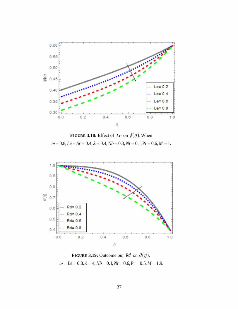
spontaneously the Sc increases and decreases. The inspiration of Le on

is illustrated by figure. 3.18, where it falls when Le is rises. Because it is ratio of

29

thermal-diffusivities to the mass diffusivities. When thermal diffusivities reduces

automatically, it reduce Le and reduce concentrations profile. The impact of

radiations Rd parameter over is shown by figure 3.19. It is simply found that

heat distribution falls with rising value of Rd . Commonly it is observe, radiating a

fluids or some others things can causes to reduce the heat of that specific objects.

3.5.1 Table Discussions

Table.1 displays numerical values of HAM solutions at different approximation

using various values of different parameters. It is clear from the table.1 that

homotopy analysis technique is a quickly convergent technique. Physical quantities

such as skin friction co-efficient, heat flux, mass flux and Local-density number of

motile microorganism for motivation of science and technology are calculate by

Tab’s: (3.2-3.5). Table: 2 displays the impact of inserting parameters and M on

Skin friction .fC It is seen that increasing value of and M decreases the skin friction

.fC Table.3 examines the influences of embedding parameters , , PrNb Nt and Rd on

heat flux .Nu

It is seen that increasing values of Pr increase the heat flux ,Nu where

, and Rd Nt Nb decrease the heat flux when it increased. Table.4 inspects the

influences of , and Le Nb Nt on mass flux .Sh The increasing values of and Le Nb

increase the mass flux where and SrNt reduces the mass flux .The influences of

, and PeSc on 0 are shown in Table.5. The increasing values of Pe increases

0 , while the higher value of and Sc reduce 0

3.5.2 GRAPHS

FIGURE 3.4: Effect of on .f When

0.8 and 1.9.M

FIGURE 3.5: Effect of on . When

0.8, 0.4, 0.1, 0.4,Pr 0.6.Le Nt Rd Nb

31

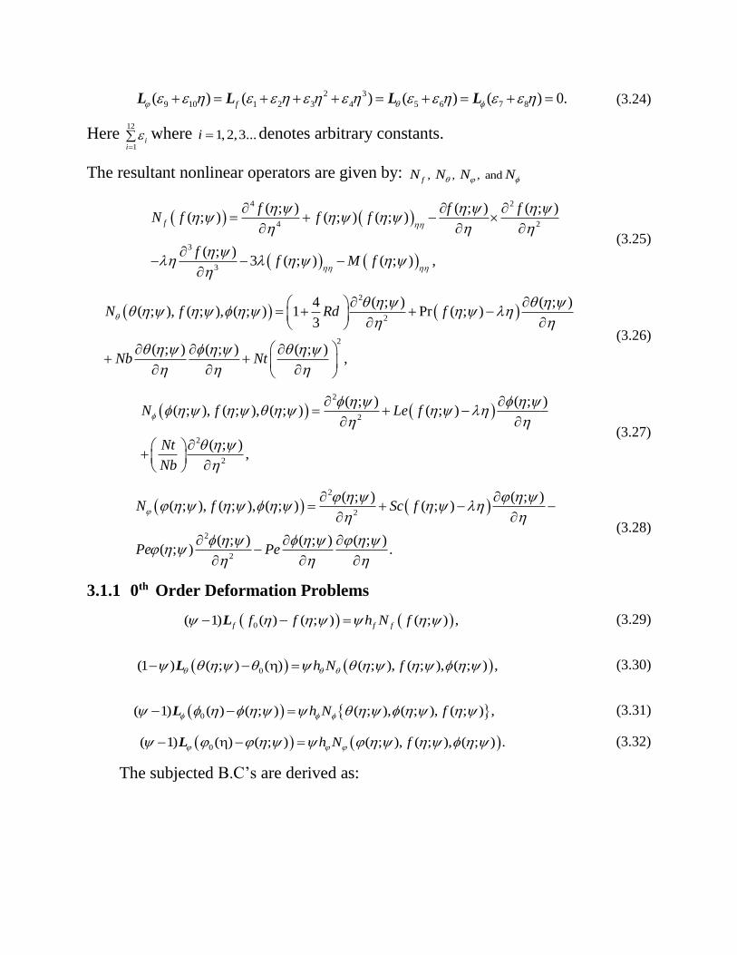
FIGURE 3.6: Outcome of our . When

0.8, 0.4, 0.1, 0.6,Pr 0.6, 0.5.Le Nt Nb M

FIGURE 3.7: Effect of on . When

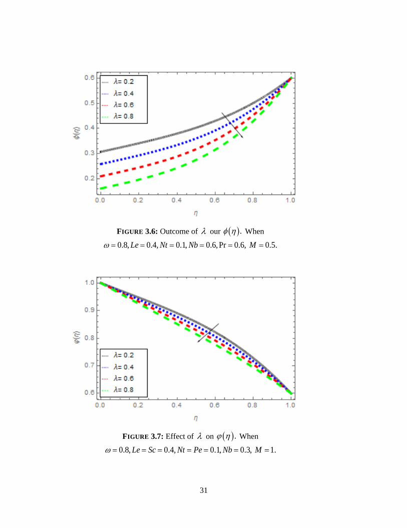
0.8, 0.4, 0.1, 0.3, 1.Le Sc Nt Pe Nb M

FIGURE 3.8: Effect of M on .f When

0.8 and 0.9.

FIGURE 3.9: Effect of M on . When

0.8, 0.3, 1, 0.6, 0.1,Pr 0.5.Le Rd Nt Nb

33

FIGURE 3.10: Effect of Pr on . When

0.8, 0.3, 0.4, 0.6, 0.1, 1.Le Rd Nt Nb M

FIGURE 3.11: Effect of Pr on . When

0.8, 0.3, 0.4, 0.6, 0.1,Pr 0.2, 1.Le Nt Nb M

FIGURE 3.12: Outcome our Nt on . When

0.8, 0.3, 0.4, 0.1,Pr 0.6, 2.Le Rd Nb M

FIGURE 3.13: Effect of Nt on . When

0.8, 0.3, 0.4, 0.1,Pr 0.6, 2.Le Nb M

35

FIGURE 3.14:Outcome our Nb on .

0.8, 0.3, 0.4, 0.1,Pr 0.6, 2.Le Rd Nt M

FIGURE 3.15: Effect of Nb on . When

0.8, 0.3, 0.4, 0.1, Pr 0.6, 1.Le Nt M

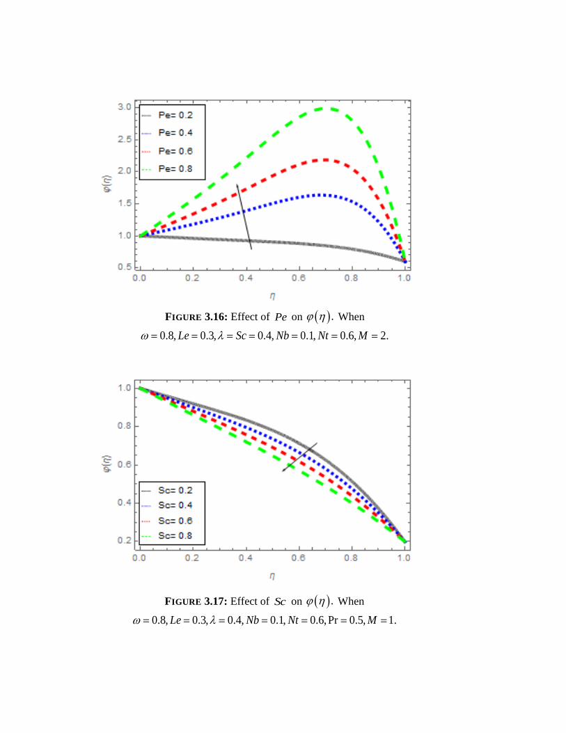
FIGURE 3.16: Effect of Pe on . When

0.8, 0.3, 0.4, 0.1, 0.6, 2.Le Sc Nb Nt M

FIGURE 3.17: Effect of Sc on . When

0.8, 0.3, 0.4, 0.1, 0.6,Pr 0.5, 1.Le Nb Nt M

37

FIGURE 3.18: Effect of Le on . When

0.8, 0.4, 0.4, 0.3, 0.1,Pr 0.6, 1.Le Sr Nb Nt M

FIGURE 3.19: Outcome our Rd on .

0.8, 4, 0.1, 0.6,Pr 0.5, 1.9.Le Nb Nt M

3.5.3 TABLES

Table. 3.2.

Numeric value of the skin-Frictions Coefficients for numerous parameter

When 1, 0.6, 0.8, 0.7Nb Nt Le Sc Pe and 0.1 .

M

1

2Ref xC

Hayat et al. [77] result

1

2Ref xC

Present results

0.1

1.5

-2.40160

1.1051

0.5

-2.41735

0.9999

1.0

-2.42522

0.9957

0.1

1.5

-2.40788

1.2057

2.0

-2.40828

1.1947

2.5

-2.40948

1.1747

3.0

-2.41426

0.9957

39

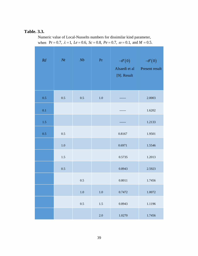
Table. 3.3.

Numeric value of Local-Nusselts numbers for dissimilar kind parameter,

when Pr 0.7, 1, 0.6, 0.8, 0.7, 0.1, and 0.5.Le Sc Pe M

Rd

Nt

Nb

Pr

0

Alsaedi et al

[9]. Result

0

Present result

0.5

0.5

0.5

1.0

------

2.0003

0.1

------

1.6202

1.5

------

1.2133

0.5

0.5

0.8167

1.9501

1.0

0.6971

1.5546

1.5

0.5735

1.2013

0.5

0.8943

2.5923

0.5

0.8011

1.7456

1.0

1.0

0.7472

1.0072

0.5

1.5

0.8943

1.1196

2.0

1.0270

1.7456

Table. 3.4.

Numeric type value of Local-Sherwoods number for dissimilar Parameter

when Le=0.6, Sc=0.8, Pr=Pe=0.7, λ=M=0.6, and ω=0.1.

Le Nb Nt 0

Alsaedi et al. [9]

result

0

Present results

0.1 0.2 0.5 0.4471 0.8518

0.5 0.5878 0.9618

0.1 0.2 0.5878 0.6624

0.6 0.9582 0.7910

1.0 1.0320 0.8518

0.2 0.5 0.5878 0.8615

1.0 0.8588 0.9020

1.5 -0.3914 0.8901

Table. 3.5.

Numeric value of Local-density-number of motilemicroorganism densities number for

numerous kinds of parameters when 0.5, Pr 1, 0.8, and 0.1,M Sc

and 0.7.Pe

Sc

Pe

0

Alsaedi et al. [9]

result

0

Present results

1.0 0.5 0.5 ------ 1.6434

1.5 ------ 1.2526

2.0 ------ 0.9542

1.0 0.5 ------ 2.1053

1.0 ------ 1.8599

1.5 ------ 0.9552

0.5 0.5 1.3811 1.6864

1.5 1.4764 1.7801

2.0 1.5731 2.1053

41

3.4 Main Observations

The problem of steady bioconvection flow between two parallel plates is studied by

assuming It is the plates capable to expand and contract. For the purpose a simple form

of similarity variables is used by reducing the supporting boundary condition in the

form. As mentioned in the previous lines that embedding parameters are graphically

presented and discussed and the different types of parameters and numbers are studied

and investigate. The base points are:

1. The concentration field of suction and injection reversely effected by

Thermophoretic and Brownian motion parameters.

2. Variation in various physical parameters and convergence of the homotopy were

numerically analysed.

3. For various bioconvectoion parameters the are precisely analysed.

4. Changes in the motile microorganisms density were analyzed for various

bioconvection parameter .

5. Skin friction .fC decrease continuesly by increasing the and M values.

6. heat flux Nu increase by increasing Pr and decrease by increasing .

7. Mass flux is in direct propotion to and Le Nbas when and Le Nb increase mass flux

also increases while mass flux reduce with Nt .

8. A very prominent variation in the density of motile microorganism observed for the

Brownian (Nb), thermophoretic (Nt) and suction/ injection parameters.

Chapter 4

Dusty Casson Nanofluid Flow with Thermal Radiation Over a

Permeable Exponentially Stretching Surface

43

4.1 Introduction

In this section, of the flows of Casson fluid on permeable exponential stretching

along with dust and liquid phase in the presence of thermal radiation. With the help

of elementary coupled and non-linear variables, the equation mostly used for fluid

velocity and thermal energy has been altered to some suitable differential equation.

Thus for the solution of model equations logical methodology has been applied. The

effect of temperature, velocity and concentration on the different types of parameters

like parameter of radiation, parameter of dust particles mass concentration,

parameter of unsteadiness and porosity, Volume fraction of dust particle and Nano

particles were studied. The impact of skin friction, Nusslet number and Sherwood

number has been outlined. Correlation is accommodated the approval of our

outcomes with previous successful works and is found in proper settlement. It has

been seen that liquid molecule connection is directly proportional to the temperature

exchange rate and is in reversely proportional to wall friction. Moreover, with

radiation parameter, the profile of dusty nano fluid is raised productively.

4.2 Formulation

Assume the unsteady 2-D thermally and electrically conducting boundary layer flow

of the dusty Casson nanofluid through porous stretching plate surface. The speed of

fluids flow over stretching surface is assumed as

0 /, exp(1 )

w

xUU x t

ct

, (4.1)

where is a exponential parameter. The flow is unsteady which start at 0t and it

became steady for 0.t The Coordinates system is selected in such a way that the

surface is along x -axis and y -axis is perpendicular on it.

The temperature source is considered non uniform where the dust particles are taken

uniform in the size. The shape of the nano and dust particles has been considered

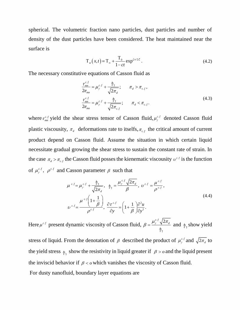
spherical. The volumetric fraction nano particles, dust particles and number of

density of the dust particles have been considered. The heat maintained near the

surface is

0 /2, exp1

.x

w x tct

(4.2)

The necessary constitutive equations of Casson fluid as

..

.

..

.

.

; ,2 2

; .2 2

c fc fmn

d c f

mn d

c fc fmn

d c f

mn c f

e

e

y

y

p

p (4.3)

where .c f

mn yield the shear stress tensor of Casson fluid, .c f

denoted Casson fluid

plastic viscousity, d deformations rate to itselfs,.c f the critical amount of current

product depend on Casson fluid. Assume the situation in which certain liquid

necessitate gradual growing the shear stress to sustain the constant rate of strain. In

the case .d c f the Casson fluid posses the kienematic viscousity .c f is the function

of . .,c f c f

and Casson parameter such that

. .. . .

.

.

. 2.

. 2

2, , ,

2

11

1, 1 .

c f c fdc f c f c f

c f

d

c f

c fc f

c f

u

y y

yy

pp

(4.4)

Here .c f present dynamic viscosity of Casson fluid, . 2c f

d

yp and yp show yield

stress of liquid. From the denotation of described the product of .

c f and 2 d to

the yield stress yp show the resistivity in liquid greater if o and the liquid present

the inviscid behavior if o which vanishes the viscosity of Casson fluid.

For dusty nanofluid, boundary layer equations are

45

0,x yu v (4.5)

2

2

11 1 ,1n d d nf pf

u u u uu КN u u

t x y y

(4.6)

,0p pu

x y

(4.7)

,p p p

p p p

u u uNm u КN u u

t x y

(4.8)

2

.p t x y nf yy pnf

qN rc T uT T k T u uy

(4.9)

The corresponding B.Cs as

, , , , , ,     y 0,

0, as, 0, .

w w w

p p

u U x t V x t T T x t where

y u T T y

(4.10)

Here the velocity & particle phase of fluid along & x y are represented by ,u

and . ,p pu The nf is dynamic viscosity and

nf is nanofluid density,

represents stokes resistance, also N and m are number density and mass

concentration of the dust particle’s respectively, where is electrical

conductivity. Also f nfc and

nfk are specific heat capacitance and effective

thermal conductivity where t denotes time.

Here 0 /, exp(1 )

w

xUU x t

ct

shows sheet velocity, c is the positive constant which

measure un-steadiness,

0 /, exp2 1

f x

w

Ux t q

tV

c

is a suction velocity, 0q for

0q injection, 0U is the suction velocity, characteristic length is ,

/20, exp1

w

xx tct

be heat distribution near the surface, 0 represent

reference heat. qr can be described under Rosseland approximation radiative

heat-flux as [36-48]:

* 4

*

4,

3qr

y

(4.11)

where * and * identifies mean absorption coefficients and Stefan-Boltzmann

constant individually. Heat differences in the flow are supposed appropriately

minor provided that 4 may be conveyed as a linear function of heat. Moreover

expanding 4 applying Taylor’s series by ignoring higher order terms yield:

4 3 44 3 , (4.12)

Furthermore, nano fluid constants are specified by [26-35]:

2.51 , 1 ,

1 1.

1

p p p nf fnp p s

s f f snf

f s f f s

c c c

n n

n

(4.13)

In order to measure nfk for various shapes of the nano particles, we assumed the

flowing formula, given by Crosser & Hamilton [78]. Here n is used for nano

particle shapes. Furthermore, 3/ 2n is for cylindrical and 3n for spherical

shapes. Volume fraction is denoted by in the nano particles. Subscript f

indicates fluid whereas subscript s indicates the solid properties.

Introducing the similarity transformations into the governing equations which

transform into the below respective coupled non-linear ordinary differential

equations:

47

12

00

12

00

12

0 0

exp ( ), exp ( ) ,1 2 1

exp ( ), exp ( ) ,1 2 1

, exp , exp .2 1 1

fx x

fx x

p p

x x

w f

UUu f E f f

ct ct

UUu g E g g

ct ct

Uy

ct ct

(4.14)

By inserting equations (4.11) to (4.14) into equations (4.6), (4.8 4.10) and

comparing the coefficients of 0

x L on both sides, we get

2111 1 1 2 2

1

2 0

d sd

f

f f ff S f f

g f f

(4.15)

2

2 2 2 0gg g S g g f g (4.16)

1 21 42Pr

3Pr 1

4 0

nf f

p pf s

Rdk k Ec g f

c c

f f S

(4.17)

The B.C’s:

, 1, 1 0,

0, g 0, g ,

0 .

f q f at

f f nf g

as

(4.18)

Here exponential parameter is , unsteadiness parameter is A where 0A Uc ,

represent mass concentration of a dust particle where

fNm , is a fluid

particle interaction parameter,

0

1Ex

f

ctM e

u

where

01 vct U , and

v m denote relaxation time of the dust relaxation time for the prandtl number

and Eckert number is Ec where 2

0 0 .p fEc U c T

For the sack of interest of the

engineers fC (friction factor) and xNu (Nusselt number) are defined as:

1 21 2 1

Re 1 1 0f xC f

(4.19)

1 2Re 0x x nf fNu k k (4.20)

Here local Reynolds number is 0Re .x fU

4.3 HAM Solution

Liao [70-76] was the pioneer who anticipated the HAM. He applied one of the

fundamental idea of the topology called Homotopy to derive the current method.

Two Homotopic functions has been used to derive present method. These functions

are known as Homotopic function when one of them is continuously distorted into

another. Assume that 1 2, are two function which are nonstop and ,X Y are

mapped from to Y then 1 is called homotopy to 2 while it gives a nonstop

functions

: 0, 1 .Y

(4.21)

x

1, 0

and 2, 1 (4.22)

Then this mapping are known Homotopic. This scheme give us auxiliary

technique and it’s mainly applied to the non-linear differential equations without

linearization and discretization.

HAM which is one of the faster and stronger convergence method. HAM is use both

strong and weak solution of nonlinear problems. Solution results found by HAM

49

hold assisting parameter which control and adjust convergence of solution as well

as bases function. The initial guess is

0 0 0( ) exp 1 , g ( ) 1 , ( ) exp .x xf q q η η η (4.23)

The linear-operators can be

3 2 2

3 2 2( ) , ( )= , ( )= .f g

f f gf g

η η η η

(4.24)

The above-mentioned differential operators satisfy the

3 1 2

4 5

6 7

( exp exp ) 0,

( exp exp ) 0,

( exp exp ) 0,

f

g

η η

η η

η η

(4.25)

Where 7

1i

i

are arbitrary constants. The resultant nonlinear operator through

, & f gN N N for the selected problem in the below given as:

23 2

3 2

( ; ), ( ; )

111 1 1 2

1

2 2 ,

f

d sd

f

f g

f f ff

S f f g f f

η ηη η η η

η η

η η η

η

(4.26)

22 2

2 2( ; ), ( ; ) 2 2 2 ,g

g g g g f gf g g S

η η η

η η η η η η (4.27)

2

2

2

1 4( ; ); ( ; ); ( ; )

3Pr 1

2Pr 4 ,

nf

fp ps f

k RdN f g

kpc pc

Ec g f f f S

η η η η η

η η ηη

(4.28)

4.3.1 0th Deformation Problem

0( 1) ( ) ( , ) ( , ), ( , )f f ff f N g f η η η η (4.29)

0( 1) ( ) ( , ) ( , ), ( , )g g gg g N f g η η η η (4.30)

0( 1) ( ) ( , ) ( , ), ( , ), ( , )N f g η η η η η (4.31)

The subjected B.Cs obtained as

( ; ) ( ; )( ; ) 0, 1, 0,

( ; ) ( ; ) ( ; )0, ( ; ) ( ; ) ,

( ; ) 1, ( ; ) 0

f ff

g f gg f n

η=0

η=0 η

η η

η η η

η=0 η

η ηη

η η

η η ηη η

η η η

η η

(4.32)

where , , 0f . The 0th order deformation problem taken as results. For 0

and 1 we get:

( ;1) ( ); ( ;1) ( ); ( ;1) ( ).f f g g η η η η η η (4.33)

Expand the non-dimensional temperature, concentration and velocity fields

( ; ); ( ; ); ( ; )f g η η η as

10

0

1 ( , )( , ) ( ) ( ) ( ) ,

!

ff f f f

ηη η η

η

MM M M

M

(4.34)

10

0

1 ( , )( , ) ( ) ( ) ( ) ,

!

gg g g g

ηη η η η

η

MM M M

M (4.35)

10

0

1 ( , )( , ) ( ) ( ) , ( ) .

!

ηη η η η

η

MM M M

M (4.36)

The axillary parameters , f and are equation series (4.29-4.31) converges at

1 , we achieve:

1

1

1

( ) ( ) ( ),

( ) ( ) ( ),

( ) ( ) ( ).

o

o

o

f f f

g g g

η η η

η η η

η η η

M M

M M

M M

(4.37)

4.3.2 thM Order

The thM order problem gratifies the succeeding equations are:

1

1

1

( ) ( ) ( ),

( ) ( ) ( ),

( ) ( ) ( ),

f

f f

g

g g

f f R

g g R

R

η η η

η η η

η η η

M M M M

M M M M

M M M M

(4.38)

51

The resultant B.Cs are

, , ,

, ,

f o f o o at o

f o g g o o as

η

η

M M M

M M M M

(4.39)

Here

1

1 1

1 10 0

1 1 1 1 1

11( ) 1 ( )

1

1 1 2

2 2 ,

df

sd n n n n

n nf

R f

f f f f

S f f g f f

η ηM M

M M

M M

M M M M M

(4.40)

1

1 1 10

1

1 1 10

( ) 2 2

( ) 2  , 

g

n nn

n nn

R S g g g g

g g f g

η

η

M

M M M M

M

M M M

(4.41)

1

1 1 1

1 1 10 0 0

1 1 1 1

1 4( ) ( )

3Pr 1

+2Pr 2

+ 4 .

nf

fp ps f

n n n n nn n n

k RdR

kpc pc

Ec g g f f g f

f f S

η ηM M

M M M

M M M M

M M M M

(4.42)

Where

1, if 1

0, if 1

M (4.43)

4.4 Numerical and Graphical Discussions

The aim of this segment of the article is to understand the effects of different

parameters which have been discussed and displayed from Figs. (4.1-4.21), Fig. 4.1

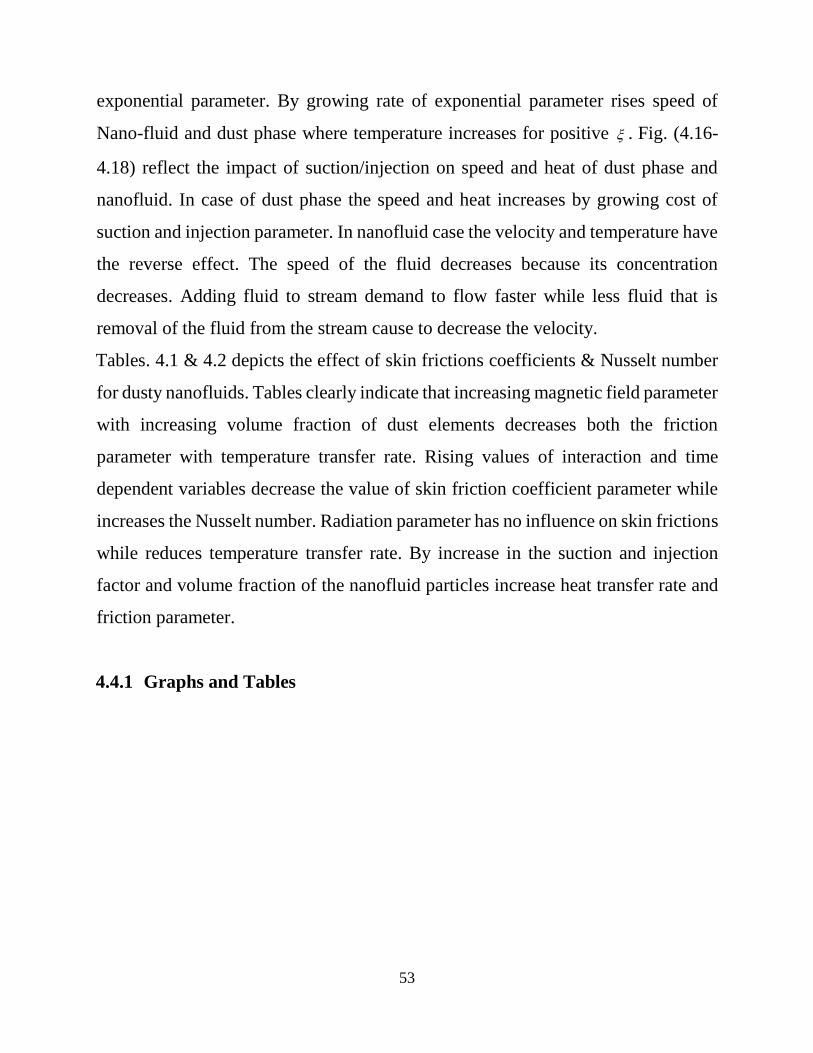
and 4.2 presented volume fraction’s impact on velocity of fluid and on dust particles.

The rise in volume fraction of the dust particles ,d decreases dust particles and

nano-fluid velocity. The density of fluid increases due to which velocity of fluid

decreases and in other words the volume to mixture ratio of dust elements is greater

than mass to dust particles. It also decreases thermal boundary layer thickniss. Fig.

4.3 and 4.4 represents the influence of volume fraction of nano particles on

temperature, velocity of Nano-particles. Graphs clearly indicate that increasing

volume fraction cause to increase the velocities of nanofluid as well as the

temperature profiles. The effect of unsteady parameter is shown in the graphs (4.5-

4.7) to rise the value of unsteady parameters it decreases the speed and warmth of

dust phase because stretching and steadiness can increase the value of velocity of

fluid. This increases the fluid velocity at the edge layer. Fig. (4.8-4.10) depicts the

influence of the interaction parameter with temperature, velocities of Nano-fluid

phase and dust particle phase. Increasing value of interaction parameter increases

velocity of dust phase and decreases velocity of nanofluid. Temperature of dust

phase rises due to growing the value of interaction parameter. The influence of

that is mass concentration on temperature and velocity of the dust phase and

nanofluid is shown in the fig. (4.11-4.13) Rise in the value of mass concentration

parameter drops the value of velocity of phase of dust and nano-fluid. Particles’

weight increase with increasing mass concentration value and due to it velocity

decreases. Fig. 4.14 describe the characteristics of magneticfiled parameter M on

velocity fields of fluids, which have a vital character in speed of the flow. It have

been perceived that growth in ,M rise the porous space which produces resistance in

path of flow and decreases motion of flow. The liquid film particles observe

obstacles in flowing above these dumps. All the way through this motion path is

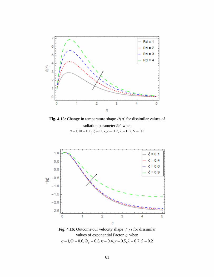
indistinct and the fluid feels retardation at every single point. The effect of Rd on

the heat distribution ( ) is obtain in the Fig. 4.15 The Rd an key role in broad

external heat conduction while the coefficient of convections temperature broadcast

is minor. If thermal radiations variable Rd is increased then it enhances the

temperature on the edge region in fluid layer. Present intensification clues to fall in

the rate of coling for the flow of nanofluids. Fig. (4.16-4.18) displayed the effect of

53

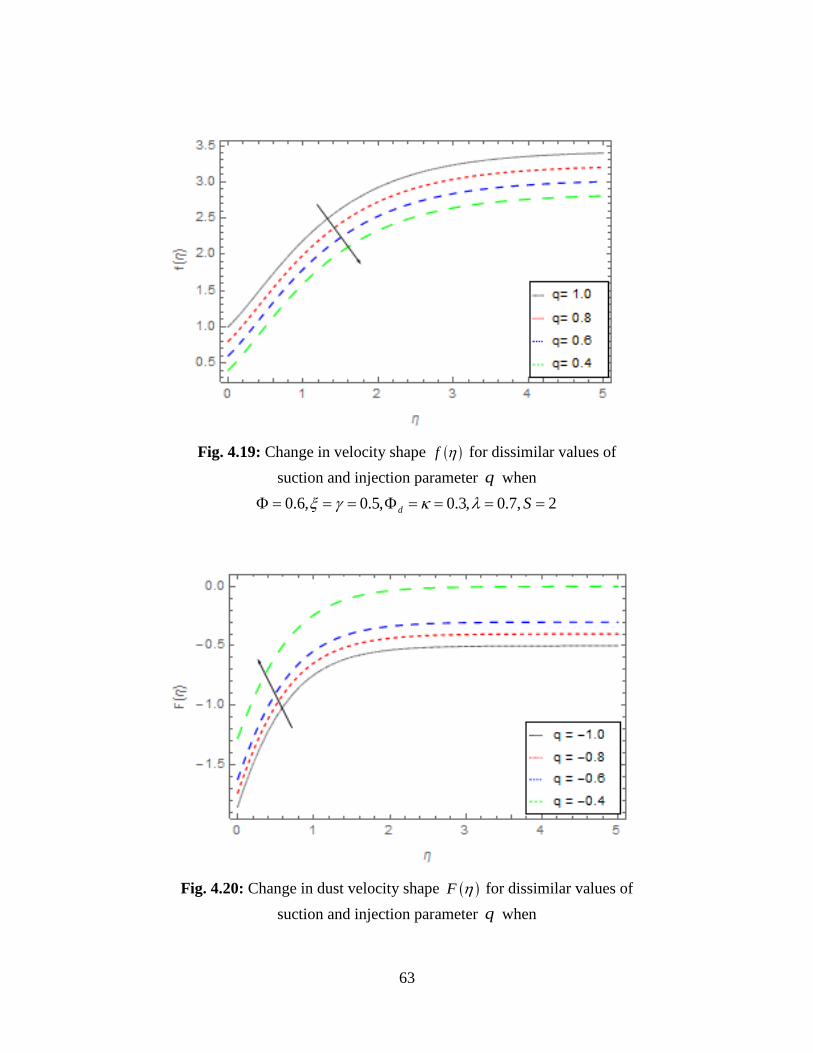
exponential parameter. By growing rate of exponential parameter rises speed of

Nano-fluid and dust phase where temperature increases for positive . Fig. (4.16-

4.18) reflect the impact of suction/injection on speed and heat of dust phase and

nanofluid. In case of dust phase the speed and heat increases by growing cost of

suction and injection parameter. In nanofluid case the velocity and temperature have

the reverse effect. The speed of the fluid decreases because its concentration

decreases. Adding fluid to stream demand to flow faster while less fluid that is

removal of the fluid from the stream cause to decrease the velocity.

Tables. 4.1 & 4.2 depicts the effect of skin frictions coefficients & Nusselt number

for dusty nanofluids. Tables clearly indicate that increasing magnetic field parameter

with increasing volume fraction of dust elements decreases both the friction

parameter with temperature transfer rate. Rising values of interaction and time

dependent variables decrease the value of skin friction coefficient parameter while

increases the Nusselt number. Radiation parameter has no influence on skin frictions

while reduces temperature transfer rate. By increase in the suction and injection

factor and volume fraction of the nanofluid particles increase heat transfer rate and

friction parameter.

4.4.1 Graphs and Tables

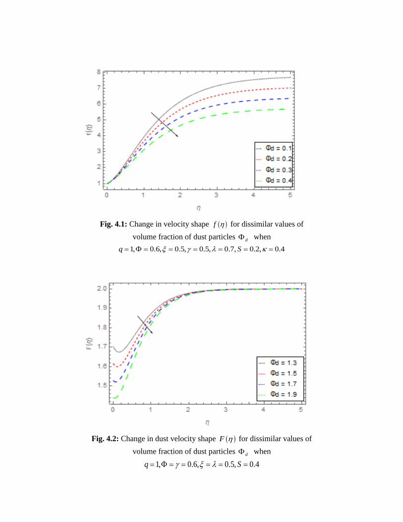
Fig. 4.1: Change in velocity shape f for dissimilar values of

volume fraction of dust particles d when

1, 0.6, 0.5, 0.5, 0.7, 0.2, 0.4q S

Fig. 4.2: Change in dust velocity shape F for dissimilar values of

volume fraction of dust particles d when

1, 0.6, 0.5, 0.4q S

55

Fig. 4.3: Change in velocity shape f for dissimilar values of

volume fraction of nanoparticles when

1, 0.5, 0.3, 0.6, 0.5, 0.7dq S

Fig. 4.4: Change in temperature shape for dissimilar values of

volume fraction of nanoparticles when

1, 0.5, 0.3, 0.7, 0.2, 0.1q Rd S

Fig. 4.5: Outcome our velocity shape f for dissimilar value of

unsteadiness factor S when

0.6, 0.5, 0.3, 0.7, 0.5d

Fig. 4.6: Outcome our dust velocity shape F dissimilar value of

unsteadiness factor S when 3, 0.6, 1.5, 0.3, 0.5dq

57

Fig. 4.7: Change in temperature shape for dissimilar values of

unsteadiness parameter S when 1, 0.6, 0.5, 0.7, 0.2, 0.1q Rd

Fig. 4.8: Change in velocity shape f for dissimilar values of

fluid particle interaction parameter when

1, 0.6, 0.3, 0.5, 0.4, 0.2dq S

Fig. 4.9: Change in dust velocity shape F for dissimilar values of

fluid particle interaction parameter when 1, 0.6, 0.5, 0.3, 0.6, 0.7dq S

Figure. 4.10: Change in temperature shape dissimilar value our

fluid particle interaction parameter when 1, 0.6, 0.5, 0.3, 0.1q Rd S

59

Fig. 4.11: Change in velocity shape f for dissimilar values of

concentration of mass of the dust particles when

1, 0.6, 0.5, 0.3, 0.7, 0.2, 0.4dq S

Fig. 4.12: Change in dust velocity shape F for dissimilar values of

concentration of mass of the dust particles when 1, 0.6, 0.5, 0.3, 0.4dq S

Fig. 4.13: Change in temperature shape for dissimilar values of

concentration of mass of the dust particles when

1, 0.6, 0.5, 0.3, 0.2, 0.1q Rd S

Fig. 4.14: Outcome our velocity shape f for dissimilar value of

Magnetic-filed factor M when

1, 0.6, 0.5, 0.3, 0.7, 0.2d

q S

61

Fig. 4.15: Change in temperature shape for dissimilar values of

radiation parameter Rd when

1, 0.6, 0.5, 0.7, 0.2, 0.1q S

Fig. 4.16: Outcome our velocity shape f for dissimilar

values of exponential Factor when

1, 0.6, 0.3, 0.4, 0.5, 0.7, 0.2dq S

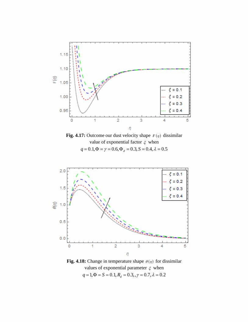
Fig. 4.17: Outcome our dust velocity shape F dissimilar

value of exponential factor when

0.1, 0.6, 0.3, 0.4, 0.5dq S

Fig. 4.18: Change in temperature shape for dissimilar

values of exponential parameter when

1, 0.1, 0.3,, 0.7, 0.2dq S R

63

Fig. 4.19: Change in velocity shape f for dissimilar values of

suction and injection parameter q when

0.6, 0.5, 0.3, 0.7, 2d S

Fig. 4.20: Change in dust velocity shape F for dissimilar values of

suction and injection parameter q when

0.6, 0.3, 0.6, 0.5, 0.4d S

Fig. 4.21: Change in temperature shape for dissimilar values of

suction and injection parameter q when

0.6, 0.5, 0.3, 0.7, 0.2, 0.1Rd S

65

Table. 4.1.

Variation in (0)fC f and (0)Nu Casson nanofluid when ( 0.2 )

Rd d S q

[79]fC

result

fC

Present

results

[79]Nu

result

Nu

Present

results

1 -1.561840 -1.77152 2.254144 4.63400

2 -1.839995 -1.77443 1.808287 4.63336

3 -2.081123 -1.77734 1.539637 4.63318

1 -1.561840 -1.77152 2.254144 4.63400

2 -1.561840 -1.77152 1.542794 3.58159

3 -1.561840 -1.77152 1.157965 3.26566

0.1 -1.561720 -1.90582 2.352369 4.40880

0.2 -1.365966 -1.83707 2.567185 4.40989

0.3 -1.265964 -1.73473 2.766619 4.41112

0.1 -1.561840 -1.76871 2.254144 4.63039

0.2 -1.649159 -1.76973 2.092565 4.62708

0.3 -1.754082 -1.77070 1.926384 4.62422

0.1 -1.123516 -1.77070 0.120926 4.63039

0.5 -1.561840 -1.78109 2.254144 4.63059

0.9 -1.918901 -1.79146 4.204056 4.63078

0.5 -1.561840 -1.77070 2.254144 2.87312

0.7 -1.747527 -1.81456 3.247056 3.57616

0.9 -1.918901 -1.85819 4.204056 4.27843

-1 -1.698309 -1.90224 1.675188 0.40880

0 -1.622546 -1.83236 1.893080 1.46096

1 -1.561840 -1.70639 2.254144 2.87612

Table. 4.2.

Variation in (0)fC g and Nu for dusty nanofluid. when ( 0.2 )

M R d S Sp

[79]fC

result

fC

Present

results

[79]Nu

result

Nu

Present

results

1 -1.541720 -1.06242 2.302369 4.63400

2 -1.817069 -1.06419 1.843278 4.63336

3 -2.056565 -1.06597 1.567336 4.63318

1 -1.541720 -1.06242 2.302369 4.63400

2 -1.541720 -1.06242 1.577610 3.58159

3 -1.541720 -1.06242 1.185285 3.26566

0.1 -1.541720 -1.06242 2.302369 4.40880

0.2 -1.345966 -1.04349 2.547185 4.40989

0.3 -1.245964 -1.03224 2.736619 4.41112

0.1 -1.541720 -1.06242 2.302369 4.63039

0.2 -1.628161 -1.06384 2.135593 4.62708

0.3 -1.732163 -1.06422 1.964310 4.62422

0.1 -1.107813 -1.06242 0.127414 4.63039

0.5 -1.541720 -1.06865 2.302369 4.63059

0.9 -1.897238 -1.07488 4.288405 4.63078

0.5 -1.541720 -1.06242 2.302369 2.87312

0.7 -1.726478 -1.08874 3.314185 3.57616

0.9 -1.897238 -1.11491 4.288405 4.27843

-1 -1.648902 -1.30986 1.729464 0.40880

0 -1.588282 -1.18329 1.944349 1.46096

1 -1.541720 -1.06242 2.302369 2.87612

67

Concluding Remarks

The present study shows transmission of temperature and flow of radiation for dusty

nano fluid flow of Casson flow in the presence of volumetric friction of nano dusty

particles on a rapid absorbing porous enlarge exterior. For the solution of model

qualities analytical techniques were also applied and the convergent were showed in

mathematical form. The impacts of implanted factors were graphically and skin

friction were numerically and graphically showed and discussed. The main points of

conclusion are:

Greater is the value of Nb greater will be the kinetic energy of nanoparticles

inside the fluid which leads to raise the heat field.

Radiation parameter Rd increment causes shrink in Thermal boundary layers

and expand the Nusselt number u .

Increment in Volume friction of Nano particles improve the temperature

transfer rate and friction factors.

Coefficient of skin friction and Nusslet number is decreased by Porosity factor

decrement.

Interaction parameters of fluid particles causes increase in temperature

transfer rate and decrease in friction factors.

Injection / suction parameter decrease heat flow profile rate.

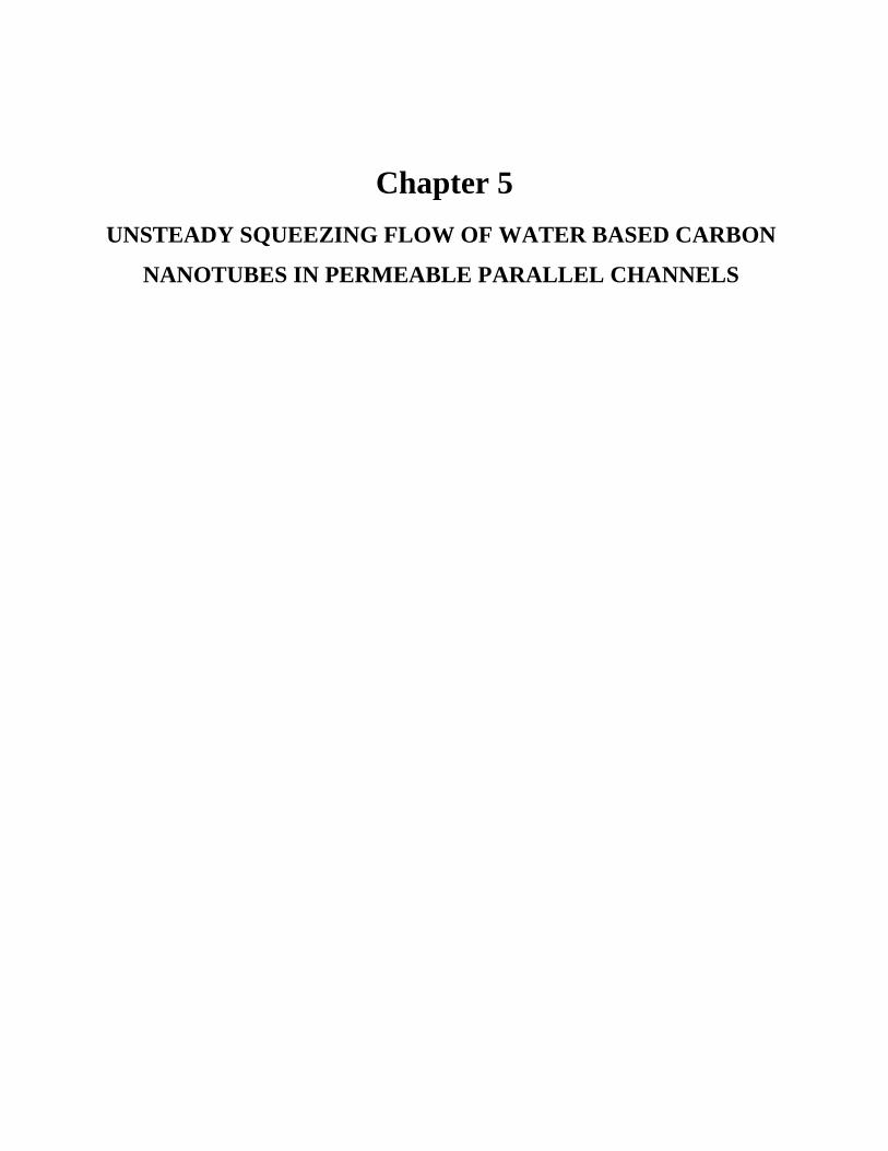
Chapter 5

UNSTEADY SQUEEZING FLOW OF WATER BASED CARBON

NANOTUBES IN PERMEABLE PARALLEL CHANNELS

69

5.1 Introduction

This subsection of thesis, we study of 3-D squeezing flow of carbon nanotube

(CNT’s) in light of water in a pivoting channel with the base wall making permeable

has been introduced. Walls are also keep permeable. Proper changes relate to solid

nonlinear Homotopy Analysis Method (HAM) illuminates normal differential

framework with the assistance of similarity factors. Graphs are present to discuss the

effect prominent physical factors on the speed and temperature.

Moreover, for different relevant variables the values for coefficient of skin friction

and Nusselt number are arranged in tabular form. The most significant after effect

of this research work is to think about the diverse practices of developing variables

on carbon nanotube (CNT’s).

5.2 Formulation of the Problem

These examination considerations on 3-measurement squeezing flows of CNTs

nanofluid (SWCNT, MWCNT nano-particles) in view of water in a pivoting disk

channel with constent & penetrable base divider. The stretching wall of the channel

is kept porous. The bottommost wall of the waterway is stretching along 0y and

beside the x axis with the velocity 1 1

w

xU

p t

. Along y-axis, the velocity of this

wall is monitored from 0

1

Vv

t

. The channel tallness is fluctuating with extending

and withering through and through of the dividers. “See Fig.1” This height change

follow fromh tv h . For the expressed issue, all the presumption and condition are

communicated in condition (5.9). The displaying of this issue is as per the following

[80];

Fig. 5.1. Geometrical portrayal of the issue.

0,x yu v (5.1)

1*

1*

2 10,

1

nf

t x y nf x xx yy

nf nf

u uu vu w up u u ut k

(5.2)

*10,

nf

t x y x xx yy

nf nf

v uv vv up v u

(5.3)

1*

1*

2 10,

1

nf

t x y nf x xx yy

nf nf

w uw vw w up w w wt k

(5.4)

0.

nf

t x y xx yy

p nf

T uT vw T TC

(5.5)

If ,   and  w u v the modules of the velocity. For *, , , , ,p nf nf nfnfC p T

demonstrate for reformed weight, kinematic-consistency, dynamic thickness,

thickness, temperature capacitance, and heat.

The limit conditions for the overhead expressed issue as pursues:

0

0.51

, , 0,  at  0,1 1

, 0, 0,  at  .1

w

VdU px dTu v T y

dw t t dw

dV p dTv u T y h t

dh t dh

(5.6)

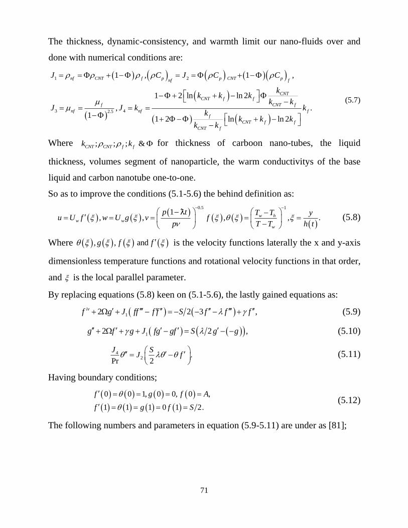
71

The thickness, dynamic-consistency, and warmth limit our nano-fluids over and

done with numerical conditions are:

1 2

3 42.5

1 , 1 ,

1 2 ln ln 2

, .1

1 2 ln ln 2

nf CNT f p p CNT pnf f

CNTCNT f f

f CNT f

nf nf ff

CNT f f

CNT f

J C J C C

kk k k

k kJ J k k

kk k k

k k

(5.7)

Where ; ; ; & CNT CNT f fk k for thickness of carboon nano-tubes, the liquid

thickness, volumes segment of nanoparticle, the warm conductivitys of the base

liquid and carbon nanotube one-to-one.

So as to improve the conditions (5.1-5.6) the behind definition as:

0.5 1

1, , , , .w h

w w

w

p t T T yu U f w U g v f

p T T h t

(5.8)

Where , ,   and   g f f is the velocity functions laterally the x and y-axis

dimensionless temperature functions and rotational velocity functions in that order,

and is the local parallel parameter.

By replacing equations (5.8) keen on (5.1-5.6), the lastly gained equations as:

12 2 3 ,ivf g J ff f f S f f f (5.9)

12 2 ,g f g J fg gf S g g

(5.10)

42 .

Pr 2

J SJ f

(5.11)

Having boundary conditions;

0 0 1, 0 0, 0 ,

1 1 1 0 1 2.

f g f A

f g f S

(5.12)

The following numbers and parameters in equation (5.9-5.11) are under as [81];

0

*

squeeze variable ,Pr Prandtl number ,

suction variable , rotation variable ,

porosity parameter .

f p f

f

CS

p k

V

ph p

pk

(5.13)

The xNu and xCf are under as follow:

12

0

0

0,nf

lowernf y y

UCf

u

(5.14)

12

00.

nf

uppernf y y h t

UCf

u

(5.15)

0

,lower

nf h w y

X T yNu Qr

k T T

(5.16)

.upper

nf h w y h t

X T yNu Qr

k T T

(5.17)

The simplifying equation (5.14-5.17), xNu and xCf are under as:

1

10.5

2.5Re 0 0,

1x lower

JCf f

(5.18)

0.5

2.5

1

1Re 1 0.

1x upper

Cf fJ

(5.19)

0.5

4Re 0 0,x lowerNu J (5.20)

0.5

4Re 1 0.x upperNu J (5.21)

Following is our required local Reynolds number Rex

dUX

dwdv

df

.

73

5.3 HAM Solution

To achieved the explanation of equations (5.9-5.11) with the B. Cs of Eq. (5.12), we

applying HAM [70-76] with the consequent route. The primary assumptions are

chosen as:

2 33( ) 2 3 1 2 , g ( ) 0, ( ) 1 .

2o o of S A A S A

(5.22)

The values L ,L and L g fare given below:

( ) ,L ( )= ,L (g)=g''.iv

f gL f f (5.23)

Having the following as:

2 3( ) L ( ) L ( ) 0,f a b c d g e h i jL e e e e e e e e (5.24)

There are ( 1 9)ie i constants general solution of the problem:

Where our model resultant nonlinear variables ,    g fN N and N are mentioned below:

2

12

( ; )( ; ), ( ; ) ( ; ) ( ; ) ( ; )

( ; )( ; ) 2 ( ; ) 3 ( ; ) 0,

2

f

fN g f J f f f

g Sf f f

(5.25)

2

2

1

( ; ) ( ; )( ; ), ( ; ) ( ; ) ( ; )

2

( ; ) ( ; ) ( ; )( ; ) ( ; ) 2 0,

g

g gN f g S g g

g f fJ f g

(5.26)

42( ; ), ( ; ) ( ; ) ( ; ) ( ; ) ( ; ) .

Pr 2

J SN f J f

(5.27)

The model 0th -order problems achieved from Equations. (5.9-5.11) as:

0( ; ), ( ; ) ( 1) ( ) ( ; ) 0,f f fN g f L f f

(5.28)

0( ; ), ( ; ) ( 1) ( ) ( ; ) 0,g g gN g f L g g (5.29)

0( ; ), ( ; ) ( 1) ( ) ( ; ) 0.N f L (5.30)

With (equivalent) sufficient B.Cs are:

1 0

0 1

0 1 1 0

( ; ) ( ; ) 1, ( ; ) , ( ; ) , 0,

2

( ; ) 0, ( ; ) ( ; ) 0, ( ; ) 1.

f S ff f A

g g

(5.31)

Where having two values 0 and 1so

( ;1) ( ), g( ;1) ( )   and  ( ;1) ( ) .g f f (5.32)

By Taylor’s series the expanding of ( ; ), ( ; ) and ( ; ) f g are described as

1

1

1

( ) ( ; ) ( ) ,

( ) ( ; ) ( ) ,

( ) ( ; ) ( ) .

q

o qq

q

o qq

q

o qq

f f f

g g g

(5.33)

Here

0 0 0

1 ( ; ) 1 ( ; ) 1 ( ; )( ) ,g ( ) and ( ) .

! ! !q q q

g ff

q q q

(5.34)

The secondary constraint show that 1 , with , and f g are a selection of such that

the above series (5.33) converges we obtained the following:

1

1

1

( ) ( ) ( ),

( ) ( ) ( ),

( ) ( ) ( ).

o qq

o qq

o qq

f f f

g g g

(5.35)

The problem thq -order fulfills below:

1

1

1

( ) ( ) ( ) ,

( ) ( ) ( ) ,

( ) ( ) ( ) .

f

f q q q f q

g

g q q q g q

q q q q

L f f U

L g g U

L U

(5.36)

The equivalent B.Cs are:

(0) 0, (0), (1) 0, (0) 0,

(1) 0, (1) 0, (0) (1) 0.

q q q q

q q q q

f f

f f g g

(5.37)

Here

75

1 1

1 1 1 1 1 1 1 1

0 0

( ) 2 3 ,2

q qiv f

q q k q k k q k q q q q

k k

Sf U J f f f f g f f f

(5.38)

1 1

1 1 1 1 1 1 1 10 0

( ) 2 ,2

q qg

q q q q q k q k k q k qk k

g g U S g g J g f f g f

(5.39)

14

2 1 1 2 10

( ) .2 Pr

q

q q q q k kk

JSU J J f

(5.40)

Where

0, if 1

1, if 1q

Main Observations

The present chapter investigation for the squeezing in 3D flow of CNTs dependent

on water based of radiation due to Temperature and MHD by utilizing homotopy

investigation strategy to be completed. MWCNTs and SWCNTs are utilized in ideal

model. Effects of implanted of variables are sketchily described.

1. With respect to MWCNTs, SWCNTs shows little resistance to the fluid.

That’s why MWCNTs have large skin resistance w.r.t SWCNTs.

2. Temperature profile is same for SWCNTs and MWCNTs with a difference

that SWCNTs has high Nusselt number against the nanoparticle volumetric

fraction.

3. Velocity profiles f in x-direction decrease with increase in A and

shows the oscillation according to increase in , and .

4. When decrement in 0S seen velocity profiles get increase and vice versa.

5. The temperature function increase with the icreasing value of S and

get reduction with the increase in and Pr .

5.4 Result and Discussions

In this segment of the dissertation, we have concisely discussed the effect of non-

dimensional numbers and emergent parameters on the functions of angular and

linear velocity , ,f f g , heat , skin-coefficient 1

2RexCf & Nusselt

numbers 1

2RexNu regarding water based MWCNTs and SWCNTs. These emerging

parameters and non-dimensional numbers are nanoparticle volume fraction , a

rotation parameter , squeeze parameter S , the suction parameter A , Prandtl

number Pr and porosity parameter respectively. Figures 5.2-5.7 are plotted to

observe the influences of these parameters. The influence of while enhancing

quantity ore , ,f f g & are depicted in Figs 5.2(a-d). Fig 5.2(a)

shows the influence on f . It can be clearly understood that in the presence of

both SWCNTs and MWCNTs, increase in the values of indicates improvement

in velocity function f in the y-direction. Consequently, the behavior of f is

dominant in cases when 0S and 0S . Due to the facts that SWCNT is more

denser than MWCNT. Fig 5.2(b) is showing the influence of our f . It can

be seen that in the interval 0 4 in the x-direction, f is showing a decreasing

trend although there is an increasing trend of f in the interval 4 1 . It must

also be noted that for 0S , the trend of f is more prominent. One can observe

the increase in rotational velocity g for 0S as depicted in figure 5.2(c). In case

MWCTs, g have higher values than SWCNTs. Also observed g have higher

values for 0S than for 0S . Figure 5.2(d) shows the relationship between and

. From here we see that the variation in is reducing with the escalating

values of . The case where the channel is contracted or the case where the channel

is stretched out, this result is identical for both cases of SWCNTs and MWCNTs.

The performance of on , ,f f g are depicted in figures 5.3(a-c). Figure

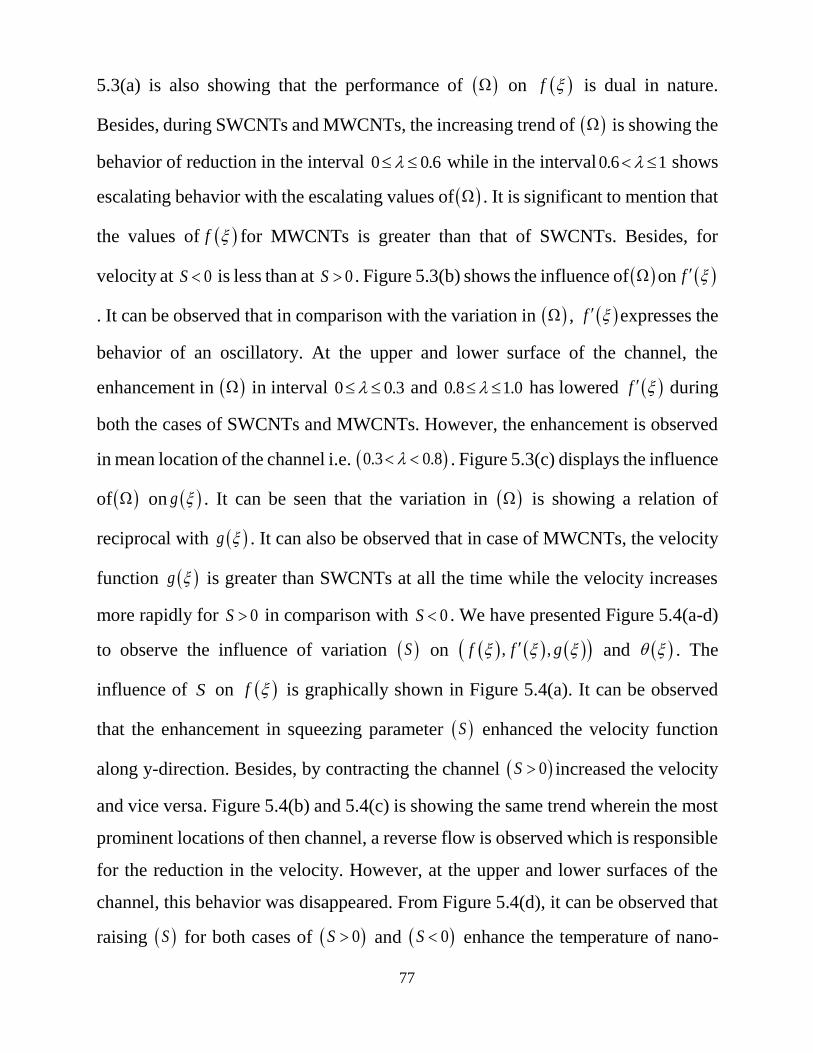
77

5.3(a) is also showing that the performance of on f is dual in nature.

Besides, during SWCNTs and MWCNTs, the increasing trend of is showing the

behavior of reduction in the interval 0 0.6 while in the interval 0.6 1 shows

escalating behavior with the escalating values of . It is significant to mention that

the values of f for MWCNTs is greater than that of SWCNTs. Besides, for

velocity at 0S is less than at 0S . Figure 5.3(b) shows the influence of on f

. It can be observed that in comparison with the variation in , f expresses the

behavior of an oscillatory. At the upper and lower surface of the channel, the

enhancement in in interval 0 0.3 and 0.8 1.0 has lowered f during

both the cases of SWCNTs and MWCNTs. However, the enhancement is observed

in mean location of the channel i.e. 0.3 0.8 . Figure 5.3(c) displays the influence

of on g . It can be seen that the variation in is showing a relation of

reciprocal with g . It can also be observed that in case of MWCNTs, the velocity

function g is greater than SWCNTs at all the time while the velocity increases

more rapidly for 0S in comparison with 0S . We have presented Figure 5.4(a-d)

to observe the influence of variation S on , ,f f g and . The

influence of S on f is graphically shown in Figure 5.4(a). It can be observed

that the enhancement in squeezing parameter S enhanced the velocity function

along y-direction. Besides, by contracting the channel 0S increased the velocity

and vice versa. Figure 5.4(b) and 5.4(c) is showing the same trend wherein the most

prominent locations of then channel, a reverse flow is observed which is responsible

for the reduction in the velocity. However, at the upper and lower surfaces of the

channel, this behavior was disappeared. From Figure 5.4(d), it can be observed that

raising S for both cases of 0S and 0S enhance the temperature of nano-

fluid in SWCNTs and MWCNTs. The influence of A on , ,f f g is

depicted in Figure 5.5(a-c). From figure 5.5(a), it can be seen that the enhancement

in A increases the velocity in y-direction. The location adjacent to the lower

portion of the channel, a prominent increase is observed because of the fluid’s

suction. It is notable that the increase in velocity due to MWCNTs is more prominent

than SWCNTs. The correlation between rate of distribution of velocity of nano-

fluid f and A is depicted in figure 5.5(b). It can be observed that there is a

reverse correlation between f and A wherein there is a decrease in f by

increasing A . It should be also observed that the reverse flow is higher for 0S

in comparison when 0S . Furthermore the f , in case of MWCNT is bigger

than SWCNT. The similar outcome is strategized for rotating velocities-distribution

g in fig. 5.5(c), by differences in g on situation of SWCNT was decreased

greater than in situation MWCNT. Figures 6(a-c) is strategized tore resents impacts

of pores on velocities distributions , ,f f g . The fig. 5.6(a) & 5.6(c)

represents decreasing behaviors in velocities function ,f g , Where in sketch

5.6(b), velocities field f displays a decline in a closed interval .4,1. . This

conduct is lads enlarging of bellow disk. In fig. 5.6(a), it remarkable to indicates the

converse flows is larger when S as matched to S . Beside, this it is seen

from the sketch that for situation of MWCNT, the velocities function

, ,f f g are constantly greater than SWCNT. the fig. 5.7 illustrates the

Pr over distribution. Heat distribution vary conversely by Pr parameter.

Boundaries layers thickness reduces with higher value of Pr variable, this

consequence is extra dispersed for smaller Pr parameter. Clearly from fig. that in

circumstance of MWCNT, heat profile constantly greater than SWCNT.

79

Fig. 5.2. (a): Change in velocity profile f for dissimilar values of

volume fraction of nanoparticles

Fig. 5.2. (b): Change in velocity profile f for dissimilar values of

volume fraction of nanoparticles

Fig. 5.2. (c): Change in velocity profile f for dissimilar values of

volume fraction of nanoparticles

Fig. 5.2. (d): Change in temperature profile for dissimilar values of

volume fraction of nanoparticles

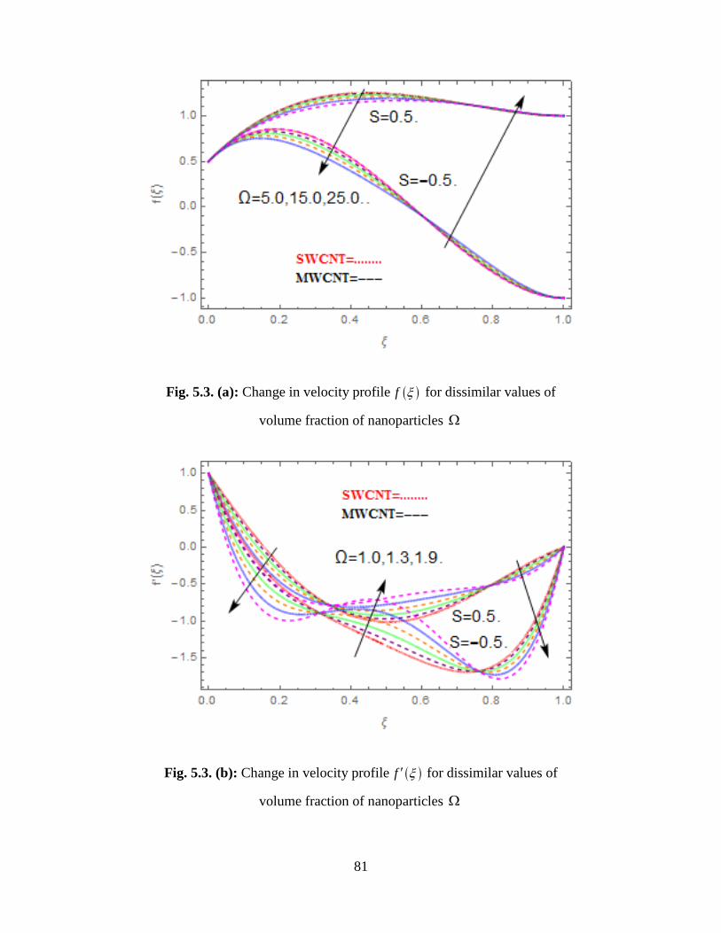
81

Fig. 5.3. (a): Change in velocity profile f for dissimilar values of

volume fraction of nanoparticles

Fig. 5.3. (b): Change in velocity profile f for dissimilar values of

volume fraction of nanoparticles

Fig. 5.3. (c): Change in velocity profile f for dissimilar values of

volume fraction of nanoparticles

Fig. 5.4. (a): Change in velocity profile f for dissimilar values of

volume fraction of nanoparticles S

83

Fig. 5.4. (b): Change in velocity profile f for dissimilar values of

volume fraction of nanoparticles S

Fig. 5.4. (c): Change in velocity profile f for dissimilar values of

volume fraction of nanoparticles S

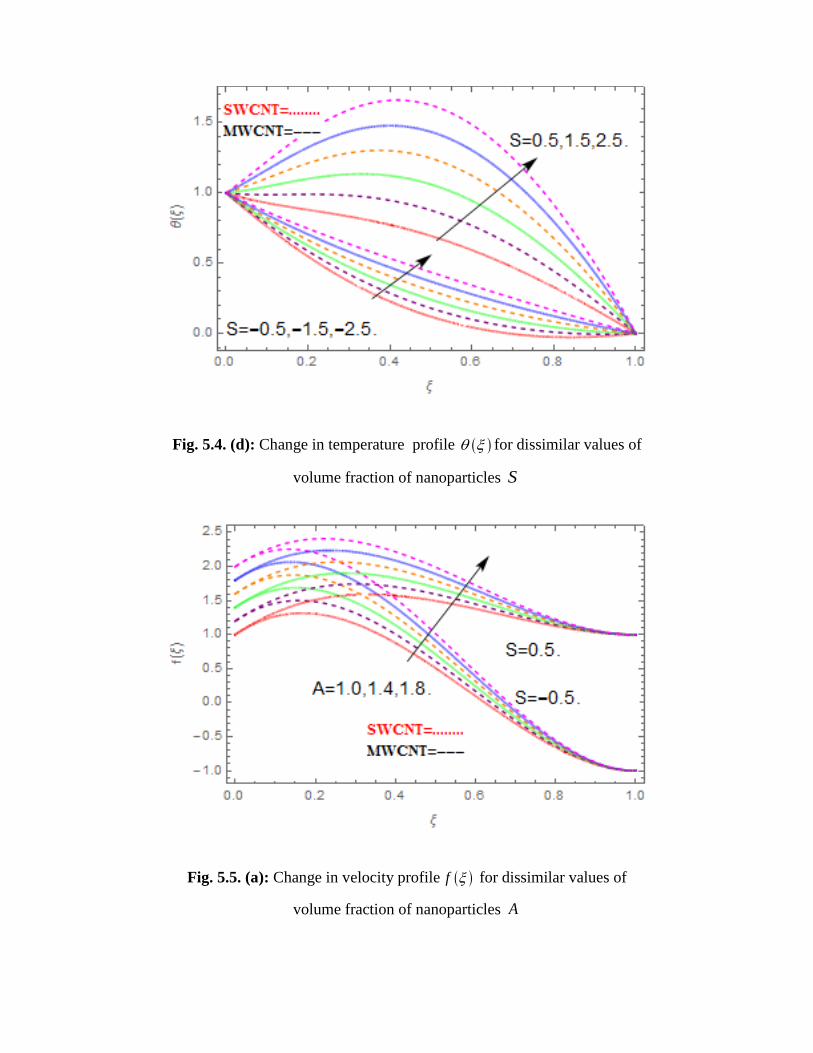
Fig. 5.4. (d): Change in temperature profile for dissimilar values of

volume fraction of nanoparticles S

Fig. 5.5. (a): Change in velocity profile f for dissimilar values of

volume fraction of nanoparticles A

85

Fig. 5.5. (b): Change in velocity profile f for dissimilar values of

volume fraction of nanoparticles A

Fig. 5.5. (c): Change in velocity profile f for dissimilar values of

volume fraction of nanoparticles A

Fig. 5.6. (a): Change in velocity profile f for dissimilar values of

volume fraction of nanoparticles

Fig. 5.6. (b): Change in velocity profile f for dissimilar values of

volume fraction of nanoparticles

87

Fig. 5.6. (c): Change in velocity profile f for dissimilar values of

volume fraction of nanoparticles

Fig. 5.7: Change in temperature profile for dissimilar values of

volume fraction of nanoparticles Pr

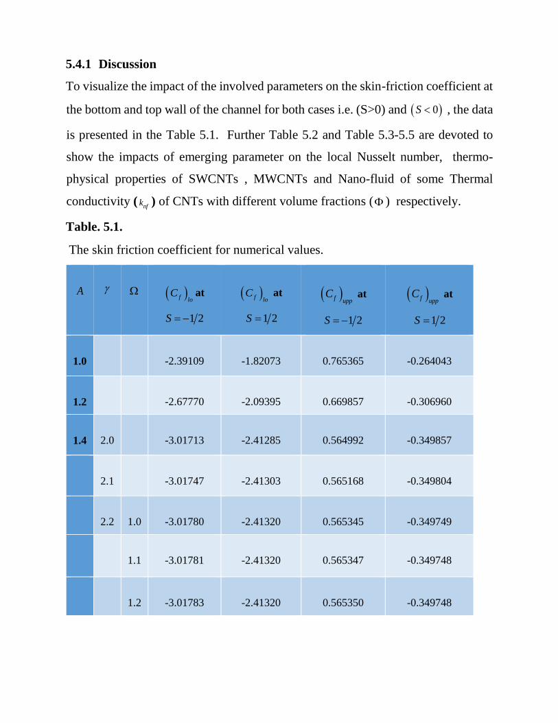
5.4.1 Discussion

To visualize the impact of the involved parameters on the skin-friction coefficient at

the bottom and top wall of the channel for both cases i.e. (S>0) and 0S , the data

is presented in the Table 5.1. Further Table 5.2 and Table 5.3-5.5 are devoted to

show the impacts of emerging parameter on the local Nusselt number, thermo-

physical properties of SWCNTs , MWCNTs and Nano-fluid of some Thermal

conductivity (nfk ) of CNTs with different volume fractions ( ) respectively.

Table. 5.1.

The skin friction coefficient for numerical values.

A

f loC at

1 2S

f loC at

1 2S

f uppC at

1 2S

f uppC at

1 2S

1.0

-2.39109

-1.82073

0.765365

-0.264043

1.2

-2.67770

-2.09395

0.669857

-0.306960

1.4

2.0

-3.01713

-2.41285

0.564992

-0.349857

2.1

-3.01747

-2.41303

0.565168

-0.349804

2.2

1.0

-3.01780

-2.41320

0.565345

-0.349749

1.1

-3.01781

-2.41320

0.565347

-0.349748

1.2

-3.01783

-2.41320

0.565350

-0.349748

89

Table. 5.2.

The local Nusselt number for the numerical values.

A

lower

Nu at

0.5S

lower

Nu at

0.5S

upp

Nu at

1 2S

upp

Nu at

1 2S

1.0 -0.159557 -0.286224 -0.097682 -0.079128

1.2 -0.158737 -0.261897 -0.073141 -0.100385

1.4 2.0 -0.147609 -0.233884 -0.051804 -0.116670

2.1 -0.147642 -0.233936 -0.051826 -0.116746

2.2 1.0 -0.147675 -0.233987 -0.051844 -0.116823

1.1 -0.162442 -0.257386 -0.057033 -0.128505

1.2 -0.177209 -0.280784 -0.062218 -0.140187

Table. 5.3.

CNTs for Physical properties.

Material

SWCNTs

MWCNTs

Thermal Conductivity

nfk

/W mK

3000

3000

Electrical Conductivity

nf

/S m

7 610 10

7 610 10

Strength Tensile GPa 100+50 =150 100+50 =150

Modulus Young’s GPa 1000+54 =1054 1000+200 =1200

Table. 5.4.

The thermophysical properties of CNTs and nano-fluid of some base fluid.

Physical Properties

Specific

Heat

1 1( / )pc kg k

Density 3

( / )kg m

Thermal Conductivity

( / )k W mk

fluid Base

Water 34.197 10 29.97 10 16.13 10

Kerosene (lamp)

oil

32.090 10

27.83 10

11.45 10

Engine oil 31.910 10 28.84 10 11.44 10

Nanofluids

SWCNT 24.25 10 32.6 10 36.6 10

MWCNT 27.96 10 31.6 10 33 10

Table. 5.5.

volume fraction ( ) with Thermal conductivities (nfk ) of CNTs different.

SWCNT fornfk

MWCNT fornfk

0.000 20.145 10 20.145 10

0.010 20.174 10 20.172 10

0.020 20.204 10 12 10

0.0300 20.235 10 20.228 10

0.040 20.266 10 20.257 10

91

Chapter 6

Conclusions

The investigated three problems in the thesis:

1. Bioconvection Model for Magneto Hydrodynamics Squeezing Nanofluid

Flow with Heat and Mass Transfer between two Parallel Plates containing

Gyrotactic Microorganisms under the Influence of Thermal Radiations

2. Dusty Casson Nanofluid Flow with Thermal Radiation Over a Permeable

Exponentially Stretching Surface

3. Unsteady squeezing flow of Water Based Carbon Nanotubes In permeable

parallel Channels

Chapter 3

In the chapter the bioconvection flow between two parallel plates is studied by

assuming It is the plates capable to expand and contract. The model of dimensional

flow have nanofluid and microorganisms and have been changed into the non-

dimensional, nonlinear system of simple differential equations. For the purpose a

simple form of similarity variables is used by reducingthe supporting boundary

condition in the form.As mentioned in the previous lines that embedding

parameteers a re graphically presented and discussed and the different types of

parameters and numbers are studied and investigate. The base points are:

An increment seen in heat profile is due to Kinetic energy of the Nanoparticles

which is because of greater value of Nb.

An increment in thermal radiation(Rd) raise the boundary layer area

temperature in the fluid which cause drop in the cooling rate of Nano fluid

flow.

Density of motile microorganism increased due to variation in

thermophoretic parameter(Nt).

The concentration field of suction and injection reversely effected by

Thermophoretic and Brownian motion parameters.

93

Variation in various phesical parameters and convergence of the homotopy

were numerically analysed.

For various bioconvectoion parameters the are precisely analysed.

Changes in the motile microorganisms density were analyzed for

various bioconvection parameter .

Skin friction .fC decrease continuesly by increasing the and M values.

heat flux Nu increase by increasing Pr and decrease by increasing .

Mass flux is in direct propotion to and Le Nbas when and Le Nb increase mass

flux also increases while mass flux reduce with Nt .

A very prominent variation in the density of motile microorganism observed for

the Brownian (Nb), thermophoretic (Nt) and suction/ injection parameters.

Chapter 4

The present study shows transmission of temperature and flow of radiation for

dusty nano fluid flow of Casson flow in the presence of volumetric friction of

nano dusty particles on a rapid absorbing porous enlarge exterior. For the solution

of model qualities analytical techniques were also applied and the convergent

were showed in mathematical form. The impacts of implanted factors were

graphically and skin friction were numerically and graphically showed and

discussed. The main points of conclusion are:

Greater is the value of Nb greater will be the kinetic energy of nanoparticles

inside the fluid which leads to raise the heat field.

Radiation parameter Rd increment causes shrink in Thermal boundary layers

and expand the Nusselt number u .

Increment in Volume friction of Nano particles improve the temperature

transfer rate and friction factors.

Coefficient of skin friction and Nusslet number is decreased by Porosity factor

decrement.

Interaction parameters of fluid particles causes increase in temperature

transfer rate and decrease in friction factors.

Injection / suction parameter decrease heat flow profile rate.

Chapter 5

The present chapter investigation for the squeezing in 3D flow of CNTs dependent

on water based of radiation due to Temperature and MHD by utilizing homotopy

investigation strategy to be completed. MWCNTs and SWCNTs are utilized in ideal

model. Effects of implanted of variables are graphically described. The main subject

theme of this research work is shown as:

With respect to MWCNTs, SWCNTs shows little resistance to the fluid.

That’s why MWCNTs have large skin resistance w.r.t SWCNTs.

Temperature profile is same for SWCNTs and MWCNTs with a difference

that SWCNTs has high Nusselt number against the nanoparticle volumetric

fraction.

Velocity profile f in y-direction increase by the increasing in value of

and A , moreover shows dual behaviour with increment and

function of Velocity decrease while with the increase in .

Velocity profiles f in x-direction decrease with increase in A and

shows the oscillation according to increase in , and .

Velocity profiles g increase by the increment, and get decrease with

the increase in , A and parameters.

When decrement in 0S seen velocity profiles get increase and vice

versa.

The temperature function increase with the icreasing value of S and

get reduction with the increase in and Pr .

95