analysis of india-sri lanka free trade...
TRANSCRIPT
HEID Working Paper No: 04/2010
An Econometric Analysis of India-Sri Lanka Free Trade Agreement
Vivek JOSHI Graduate Institute of International Studies
Abstract
This paper investigates whether the India-Sri Lanka Free Trade Agreement (ISLFTA)
has had trade creation or trade diversion effects on the rest of the World. The method
used resembles the one used by Romalis (2005) to study NAFTA. In order to use the
variations in tariff at the product level, we use six digit HS classification of products.
We construct seven panel data sets for the period 1996 to 2006. We use the commodity
and time variation in the tariff preferences allowed under ISLFTA, to identify its effect
on sourcing of different products from ‗control country‘ to ISLFTA region. Using fixed
effects model we find that the ISLFTA has been minimally trade creating for control
countries.
© The Authors.
All rights reserved. No part of this paper may be
reproduced without the permission of the authors.
2
An Econometric Analysis of India-Sri Lanka
Free Trade Agreement
Vivek Joshi1
March, 2010
Abstract
This paper investigates whether the India-Sri Lanka Free Trade Agreement (ISLFTA)
has had trade creation or trade diversion effects on the rest of the World. The method
used resembles the one used by Romalis (2005) to study NAFTA. In order to use the
variations in tariff at the product level, we use six digit HS classification of products.
We construct seven panel data sets for the period 1996 to 2006. We use the commodity
and time variation in the tariff preferences allowed under ISLFTA, to identify its effect
on sourcing of different products from ‗control country‘ to ISLFTA region. Using fixed
effects model we find that the ISLFTA has been minimally trade creating for control
countries.
Keywords: Free trade agreement, tariffs, trade creation.
JEL classification: F10, F13, F15
1 Graduate Institute of International and Development Studies, Avenue de la Paix 11A, CH-1202 Geneva,
E-mail: [email protected]. I gratefully acknowledge the valuable advice and guidance by
my supervisor Richard Baldwin. I sincerely thank Patrick Low, John Cuddy and Jaya Krishnakumar for
their helpful comments on the draft of the paper. I also thank Theresa for her continuous intellectual
inputs throughout this study. Last but not least, I acknowledge support from Swiss National Centre of
Competence in Research (NCCR, Trade) for this paper.
3
1 Introduction
The growth of regional trade blocs has been one of the major developments in
international relations in recent years. During the 1990s, regionalism was conceived as a
developmental option in itself that would promote competitiveness of trade bloc
members and help their fast integration into the international economy. As per the
World Bank report on ‗Global Economic Prospects‘ (2005) the number of the Regional
Trade Agreements (RTAs) has more than quadrupled since 1990 rising to around 230
by late 2004 and the trade between RTA partners now constitutes nearly 40% of total
global trade. Quoting, World Trade Organisation (WTO) this report estimates another
60 agreements at various stages of negotiations. The World Bank report points out that
the boom in Regional Trade Agreements (RTAs) reflects changes in certain countries‘
trade policy objectives, the changing perceptions of the multilateral liberalization
process, and the reintegration into the global economy of countries in transition from
socialism.
Regional agreements vary widely, but all have the objective of reducing barriers to trade
between member countries—which implies discrimination against trade with other
countries. At their simplest, these agreements merely remove tariffs on intra bloc trade
in goods, but many go beyond that to cover non-tariff barriers and to extend
liberalization to investment and other policies. At their deepest, they have the goal of
economic union and involve the construction of shared executive, judicial, and
legislative institutions. Many factors, some explicitly stated and others not so publicly
admitted, have been responsible for the recent spurt in regionalism. The desire to put the
multilateral system into faster and deeper action in selected areas by creating more
powerful blocs that would operate within the GATT/WTO system2 and the fear of being
left out while the rest of the world swept into regionalism, the domino effect are often
cited as the major reason for the growth of RTAs. After China‘s entry into WTO , the
2 Article XXIV of the GATT, 1994 imposes three basic obligations on WTO members wishing to enter
into a Free Trade Agreement (FTA) covering trade in goods--- i) An obligation to notify the FTA to the
WTO; ii) An obligation not to raise the overall level of protection and make access of products of third
parties not participating in the FTA more onerous (the so-called external trade requirement); and iii) An
obligation to liberalize substantially all the trade among constituents of the FTA (the so-called internal
trade requirement).

4
East Asia has experienced a massive domino effect with dozens of new RTAs being
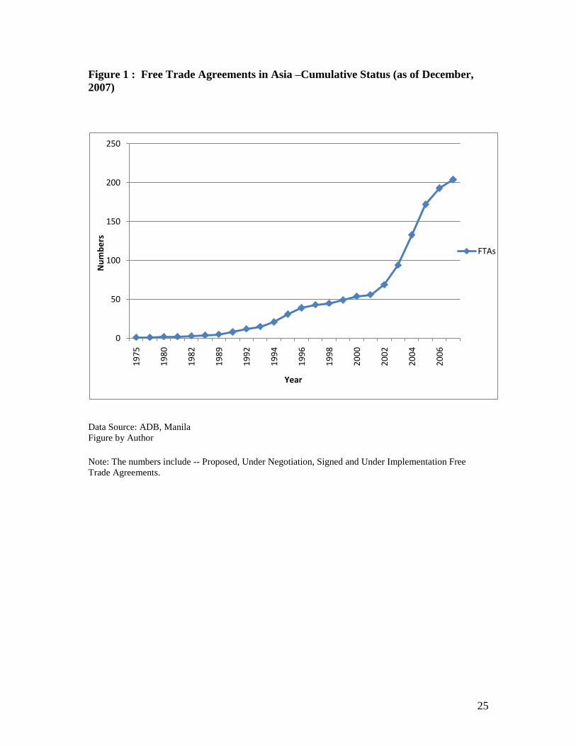
announced, negotiated and signed (Baldwin 2006). The growth of Free Trade
Agreements (FTAs) in Asia as estimated by Asian Development Bank (ADB) is shown
Figure 1.
Political considerations also features in decisions to establish RTAs, especially when
governments seek to consolidate peace and increase regional security as well as to
acquire greater bargaining power in multilateral negotiations by first tying in partner
countries through regional commitments.
There has been considerable debate in academic circles about the impact of RTAs on
the member countries and on the rest of the world (Bhagwati and Krueger; Krueger
1997). One view for RTAs has been that they improve resource allocation within a
region and improve income for member countries by reducing the trade barriers.
Consumers are better off as they can buy the goods form the most efficient supplier at
the lowest cost. This is so called trade creation effect for the members. On other hand,
the arguments are given that by its nature, an RTA is discriminatory for the non-
members and members gain at the expanse of the non-members, resulting into trade
diversion. In general an RTA would lead to some amount of both trade creation and
trade diversion effects (Krueger 1997). If the trade diversion is sufficiently large
relative to the trade creation effects, the RTA could conceivably end up being harmful
to the member countries.
In this research paper, we empirically analyze the ―India-Sri Lanka Free Trade
Agreement‖ (ISLFTA) to find out the trade creation or diversion effects of ISLFTA on
rest of the world. We use the detailed trade data (HS 6 digit level) to study the trade
effects under ISLFTA. The reason for choosing this FTA is that it is one of the few
South-South Agreements that is working credibly and could be an example for other
South-South Agreements to emulate. Holmes (2005) for example, also found that India
Sri Lanka FTA is an effective Regional Trade Agreements and one of few effective
South-South Agreements. Using gravity model she tested 122 FTAs and found that only
46% of FTAs (including ISLFTA) were effectively implemented, in the sense that they

5
positively and significantly increased the trade flows between member countries. The
success of ISLFTA has proved that if the concerns of smaller economy are taken into
account with more favorable treatment then the size differential in the economies of the
FTA partners do not matter. Being the first of its kind in the South Asian region, it has
invited lot of interest among the exporters of the region.
This paper is organized as follows: Section 2 gives a brief outline of ISLFTA , using
trade flows makes an assessment about the effectiveness of this Agreement, Section 3
presents Literature Review, Section 4 discusses the Methodology used for analysis of
ISLFTA, Section 5 gives a brief outline of the theoretical model, Section 6 describes the
data sources and limitations of data, Section 7 covers econometric issues and discusses
the results, and finally, Section 8 concludes the paper summarizing the major finding of
this study.
2 Assessment of Trade under the ISLFTA
The India Sri Lanka FTA was signed in 1998 and became operational in March 2000.
Mutual phased tariff concessions on different products on 6 digit Harmonised
Classification3 (HS Code) basis have been granted by both the partners. Each side is
having its negative lists4 (no concessions), positive list (immediate full concessions) and
a residual list5 (phased tariff reductions)
as per the framework of ISLFTA. The
preferential trade under the FTA is governed by Rules of Origin6, which specify the
3 The Harmonised Commodity Description and Coding System, commonly referred to as the
‗Harmonised System‘ or HS, is an international commodity classification system developed under the
auspices of the Brussels-based Customs Cooperation Council (CCC), known today as the World Customs
Organization (WCO). The Harmonised System consists of 21 sections covering 99 Chapters, 1,241
headings and over 5,000 commodity groups. 4 Items, which are considered sensitive to the domestic industry by each partner to FTA, are included in
the respective negative list. The items in negative list of Sri Lanka are not entitled for any duty
concessions for imports from India. The same rule applies in case of India‘s negative list for Sri Lankan
products. 5 The positive list and residual list are considered less sensitive to domestic interests by each partner and
are included in the phased reduction of tariffs by both sides. All the three lists in respect of India and Sri
Lanka are available on Sri Lanka‘s Department of Commerce website.
http://www.doc.gov.lk/web/indusrilanka_freetrade.php. 6 The customs duties applied to imported goods may differ depending on the country from which the
goods were exported. Most industrial products, available on the market today, are produced in more than
one country. For example, in the case of cotton shirts, it is possible that the cotton used in their
production is manufactured in country A, the textile woven, dyed and printed in country B, the cloth cut
6
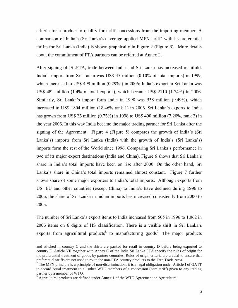
criteria for a product to qualify for tariff concessions from the importing member. A
comparison of India‘s (Sri Lanka‘s) average applied MFN tariff7 with its preferential
tariffs for Sri Lanka (India) is shown graphically in Figure 2 (Figure 3). More details
about the commitment of FTA partners can be referred at Annex I .
After signing of ISLFTA, trade between India and Sri Lanka has increased manifold.
India‘s import from Sri Lanka was US$ 45 million (0.10% of total imports) in 1999,
which increased to US$ 499 million (0.29% ) in 2006; India‘s export to Sri Lanka was
US$ 482 million (1.4% of total exports), which became US$ 2110 (1.74%) in 2006.
Similarly, Sri Lanka‘s import form India in 1998 was 538 million (9.49%), which
increased to US$ 1804 million (18.46% rank 1) in 2006. Sri Lanka‘s exports to India
has grown from US$ 35 million (0.75%) in 1998 to US$ 490 million (7.26%, rank 3) in
the year 2006. In this way India became the major trading partner for Sri Lanka after the
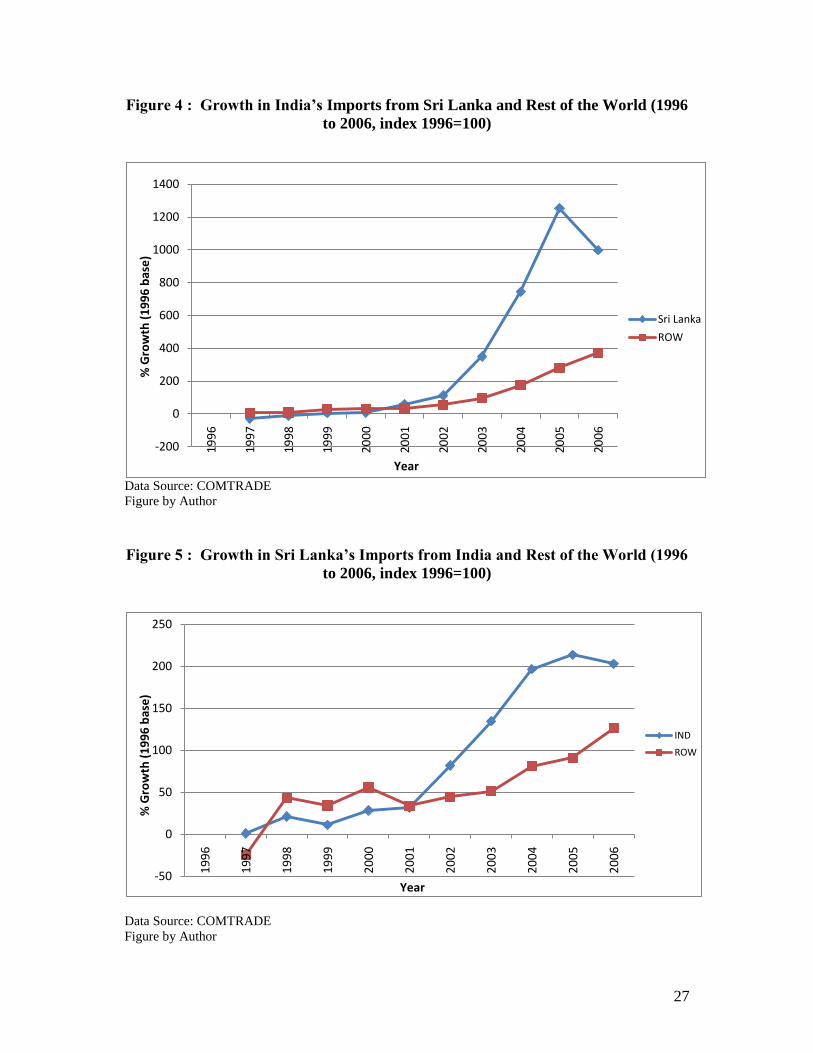
signing of the Agreement. Figure 4 (Figure 5) compares the growth of India‘s (Sri
Lanka‘s) imports from Sri Lanka (India) with the growth of India‘s (Sri Lanka‘s)
imports form the rest of the World since 1996. Comparing Sri Lanka‘s performance in
two of its major export destinations (India and China), Figure 6 shows that Sri Lanka‘s
share in India‘s total imports have been on rise after 2000. On the other hand, Sri
Lanka‘s share in China‘s total imports remained almost constant. Figure 7 further
shows share of some major exporters to India‘s total imports. Although exports from
US, EU and other countries (except China) to India‘s have declined during 1996 to
2006, the share of Sri Lanka in Indian imports has increased consistently from 2000 to
2005.
The number of Sri Lanka‘s export items to India increased from 505 in 1996 to 1,062 in
2006 items on 6 digits of HS classification. There is a visible shift in Sri Lanka‘s
exports from agricultural products8 to manufacturing goods
9. The major products
and stitched in country C and the shirts are packed for retail in country D before being exported to
country E. Article VII together with Annex C of the India Sri Lanka FTA specify the rules of origin for
the preferential treatment of goods by partner countries. Rules of origin criteria are crucial to ensure that
preferential tariffs are not used to route the non-FTA country products to the Free Trade Area. 7 The MFN principle is a principle of non-discrimination; it is a legal obligation under Article I of GATT
to accord equal treatment to all other WTO members of a concession (here tariff) given to any trading
partner by a member of WTO. 8 Agricultural products are defined under Annex 1 of the WTO Agreement on Agriculture.
7
exported by Sri Lanka to India in 2006 included – Fats and Oils (22.3%), Copper and
Articles of Copper (8.6%), Electrical Machinery (8.6%) and Spices, Coffee, Tea
(6.2%). Similarly, India exported Mineral Fuel, Oil (22.44%), Vehicles (18.08%), Iron
and Steel (4.54%), Machinery, Reactors, Boilers (4.22%) and Pharmaceutical Products
(4.13%) to Sri Lanka.
Figure 8 shows share of Sri Lankan products in India‘s total imports. It also shows Sri
Lanka‘s share in India‘s imports in items under three lists- negative, residual and
positive lists. As mentioned before, there has been an increase in total share of import of
Sri Lankan goods from 0.10% in 1999 to 0.29% in 2006. The import from Sri Lanka
has also increased in the items on the residual list from 0.2% in 1996 to 0.47% in 2006.
It is noteworthy that there has been an increase in the imports even in the negative list
items from 0.5% in 2001 to 1.19 % in 2006. This could be mainly due to the increased
awareness to partners‘ market, smoothening of customs issues and improved access to
ports of entry due to the increased engagement of partner countries on products having
preferential tariffs on residual list, the so called ‗border effects‘ .
However, the trade flows in the positive list items is relatively stagnant. This could be
attributed to the fact that during ISLFTA negotiations, the immediate concessions were
allowed by India on the products on which Sri Lanka does not have a comparative
advantage. Same could be said about the items on Sri Lanka‘s positive list. This is a
good strategy by both the countries to prepare their domestic industry for smooth
adjustments due to FTA and make ISLFTA a workable agreement.
All the above facts clearly show a marked increase in trade flows between India and Sri
Lanka after implementation of ISLFTA in 2000. Trade creation between members and
new products entering Indian market from Sri Lanka is evident after ISLFTA. But we
remind the reader that in this study, we will be limiting our econometric analysis to find
trade creation or trade diversion effects of ISLFTA on rest of the world.
9 Products other than agricultural products can be categorized as manufactured or non-agricultural
products. The product classification under non-agricultural products is still being discussed at Non
Agricultural Market Access (NAMA) negotiations at WTO.

8
3 Literature Review
Despite its importance in the South Asian region, not many empirical studies have been
conducted to access the impact of ISLFTA. We know only one study, which has
attempted to analyses the performance of this FTA by Mukerji and Kelegama (2007).
Their study is based on the bilateral trade flows under different categories of products.
Sector wise imports and exports figures are compared before and after the FTA. They
have concluded that the two countries have displayed political will to forge ahead
towards economic integration and the considerable size disparity between the two
economies does not hinder bilateral free trade when appropriate special and differential
treatment is accorded to the smaller country. Some new goods from Sri Lanka have
found entry into the Indian market following the exchange of preferences. Finally, they
have concluded that the economic benefits of free trade can and do override political
problems. In the previous version of their study Mukerji, Kelegama and Jayawarhana
(2004), they have found modest increase in trade in case of overall Indian imports from
Sri Lanka, but considerable trade increase in case of Sri Lankan imports from India.
Another report on evaluating economic performance of the FTA is ‗Joint Study Group
on India –Sri Lanka Comprehensive Economic Partnership Agreement‘ constituted by
the partner Governments (JSG report, 2003)10
. JSG (2003) has concluded that ISLFTA
promoted a 48% increase in bilateral trade between 2001 and 2002, and at present India
is the largest source of imports into Sri Lanka, accounting for 14% of Sri Lanka‘s global
imports. India is the fifth largest export destination for Sri Lankan goods accounting for
3.6% of Sri Lanka‘s global exports. Based on the success of ISLFTA, the JSG has
recommended that the two countries enter into a Comprehensive Economic Partnership
Agreement (CEPA) covering trade in services and investment and to build upon the
ISLFTA by deepening and widening the coverage and binding of trade in goods.
Most of the sophisticated econometric analysis of FTA has been on NAFTA. In order to
decide about our methodology for this study, we surveyed studies conducted in the
10
JSG (2003) can be found at
http://www.ips.lk/news/newsarchive/2003/20102003_islcepa_final/islcepa.pdf#search='India%20Sri%20
Lanka%20Trade%20Study'

9
context of NAFTA, as we could draw a parallel to the NAFTA‘s trade analysis for our
research. Most of these studies have examined aggregate imports and exports, but there
are only few studies focusing on disaggregate trade data.
For example, Gould (1998) adopted a gravity model to find the impact of NAFTA on
North American trade. Using aggregate quarterly trade flows in log first differences, he
concluded that NAFTA may have stimulated the growth of US aggregate exports to
Mexico but not US imports from Mexico. Gould (1998) also finds no trade diversion. In
another gravity based approach, Soloaga and Winters (2001) find no distinguishable
evidence of trade diversion on non-members of NAFTA. Similarly, Krueger (1999,
2000), also adopted a gravity model approach and finds no evidence of trade diversion
from the rest of the world after NAFTA came into operation. She finds that events other
than NAFTA, such as Mexico‘s real exchange rate and its trade liberalization process,
appear to have dominated the pattern of trade. Fukao, Okubo and Stern (2003) focused
on disaggregated level (2 digit ) for selected manufactured goods , using a version of the
gravity model developed for the percentage of imports from a country to US total
imports of an industry. Out of 60 sectors examined, they find evidence of trade
diversion in the textile and apparel sector, where Mexican exports have replaced lower-
cost Asian exports. This is in agreement with the findings of USITC (2003) study that
also found evidence of trade diversion in one sector (apparel) out of 68 sectors
analyzed.
The most ambitious study of NAFTA on highly disaggregated (HS 6 digit) is by
Romalis (2005). This study is based on the estimation of effects of FTA on trade
volumes and prices. It identifies demand elasticities by developing a difference in
differences based method that exploits the variation across commodities and time in the
US tariff preference given to goods produced in other NAFTA countries. It also
identifies the supply elasticities by using tariffs as instruments for observed quantities.
With the estimates of demand and supply elasticities, he estimates the change in welfare
and trade due to NAFTA. He finds that 25-30% of the rise in Mexican exports to US
since 1993 is due to Mexico‘s improved preferential treatment, implying substantial
trade diversion. The welfare analysis of Trade Volumes is followed by Econometric
10
Confirmation of Trade Diversion and its role in reducing the static welfare gains.
Romalis (2005) develops a log difference equation of value of exports of commodity z
from a non-NAFTA country (control country c’) to North America (country 1) and to
the EU (country 2), grossed up for transport costs and tariffs. He regresses the log-
difference between ‗country 1‘ and ‗country 2‘ imports from control country c’ on
preferential and MFN tariffs to estimate the trade diversion/creation.
4 Methodology for Analysis of ISLFTA
To find the trade creation or trade diversion effects of the India- Sri Lanka Free Trade
Agreement (ISLFTA) on rest of the World, we follow a slightly modified methodology
adopted by Romalis (2005)11
. Ideally, we should also estimate the demand and supply
elasticities for our key countries, for which we will need item-wise data on domestic
production and consumption of goods. But Governments in India or Sri Lanka do not
maintain such data on six digit HS, so we are unable to estimate these two parameters
for our study.
In order to use the variations in tariff at the product level like Romalis, we use 6 digit of
HS 1996 product classification in our analysis. We choose India and Sri Lanka, (the
ISLFTA partners --‗country 1‘)12
as our key countries. We first choose China as
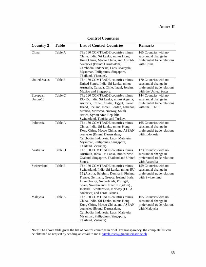
‗country 2‘ and 165 countries grouped together as control country c’ (Annex II, Table
A) to estimate the Trade Diversion/Creation due to ISLFTA. The choice of China as
‗country 2‘ to identify trade diversion is of minor significance to the empirical analysis.
China was chosen for two main reasons. Firstly, its detailed trade data has been
available electronically. Secondly, China is having significant trade with for both of our
key countries. The choice of China is further due to the reason that, it has substantial
trade with most of the control countries c’ (Annex II Table A) but it does not have any
substantial change in preferential trade relations with these countries during the study
period (1996-2006). Control countries are the countries form the rest of the world, who
have not changed their preferential trade relations substantially with either ISLFTA
11
Romalis J. (2005), ―NAFTA‘s and CUSFTA‘s Impact on International Trade‖, NBER WP11059,
Cambridge. 12
In this study, we will use the word country to mean often a group of countries. For example, India and
Sri Lanka together are referred as ‗country 1‘ and Annex Table A to E countries as control country c‘.
11
partners or China during 1996 to 2006. We selected the control countries from the list
of 180 countries supplying data to COMTRADE during the study period. We dropped
from this list the countries having special trade relationship with China during the study
period--- Hong Kong, Macau and 10 ASEAN countries (Brunei Darussalam, Cambodia,
Indonesia, Laos, Malaysia, Myanmar, Philippines, Singapore, Thailand, Vietnam).
Again, we dropped China, India and Sri Lanka (our key countries). Further we deleted
from the list European Union, as the individual member countries of EU are already
covered in our list. This gives us a list of 165 countries as the control countries c’ for
this study. (Annex II Table A).
We use the commodity and time variation in the tariff preferences allowed under
ISLFTA, to identify the ISLFTA‘s effect on sourcing of commodities from a non-
ISLFTA country c’ (control countries) to ISLFTA partners(country 1) and China
(country 2). The idea is when FTA causes a preferential treatment to the Sri Lankan
goods, the consumers in India, tend to substitute the preferential goods for the goods
from other sources (including the domestic production). Similarly, the Sri Lankan
consumer will substitute the goods of Indian origin, if they have preferential treatment
compared to the goods from rest of the trading partners. On the other hand, for the
goods, where the ISLFTA does not offer new preference (i.e. when the MFN tariff rates
are almost zero), the impact of ISLFTA comes through the ‗border effects‘ that go
beyond the tariff liberalization, as could be seen from the increased import volumes of
commodities on ISLFTA negative list.
In order to ensure the robustness of our results, in the second part of our analysis, we
use 6 other countries as ‗country 2‘. We select ‗country 2‘ based on the principle
mentioned above (i.e. when choose ‗country 2‘ as China). We choose United States
(US), European Union (EU15) , Indonesia, Australia, Switzerland and Malaysia for this
purpose. The Control Countries c‘ for US, EU15, Australia and Switzerland are listed in
Annex II Table B (170 countries), Table C (144 countries), Table D (173 countries),

12
Table E (159 countries) and respectively. The control countries when we choose
Indonesia or Malaysia as our ‗country 2‘ are in Annex II Table A (165 countries)13
.
5 Theoretical Framework and Empirical Strategy
In this section, we provide a short outline of the model, which rather than being
exhaustive, highlights the needed features for the empirical strategy14
. In this model, the
firms are assumed to produce goods under the perfect competition. Trade is assumed to
be driven by varieties and the commodities are differentiated by its source of origin.
The FTA causes a shift in sourcing of varieties by consumers by substituting the goods
from the source having preferential access to the FTA partners‘ market.
In every period t consumers in each country c are assumed to maximize Cobb-Douglas
utilities of their consumption of the output of each industry ( )ctQ z with the fraction of
income spent on industry z being ( )cb z .
The utilities for consumers in country c are as:
1
0
( ) ln ( )ct c ctU b z Q z dz (1)
1
0
( ) 1cb z dz (2)
The outputs of a country‘s firms are identical products, but different countries produce
different products in the same industry. ( )ctQ z can be interpreted as a sub-utility
function that depends on the quantity of each variety of z consumed. ( )ctQ z is defined
as under:
13 The control countries, when we choose Indonesia or Malaysia as our ‗country 2‘ are same as those
when ‗country 2‘ chosen is China (Table A) . This is due to the fact that both Indonesia and Malaysia are
among the ten ASEAN countries having preferential trade relations with China. 14
Here we focus on demand side only. For complete equilibrium analysis for FTA, Romalis (2005) may
be referred.

13
1 1
'
'
( ) ( )
z
z z
z
ND
ct ct c
c
Q z q z (3)
where, elasticity of substitution z > 1 and '( )D
ct cq z denote the quantity consumed in
country c of commodity z produced in country c’.
The demand function in country c, for a commodity z from country c’, '( )D
ct cq z is
assumed to be a CES function. The demand for 'cz is assumed to depend on seven
variables -- '( ( ))s
t t ca q z : the marginal cost of production of commodity in country c’;
'( ) 1ct cz : the ad-valorem tariff15,16
imposed on z from c’ by country c; '( )ct cg z :
transport costs for international trade; ˆctzP : the ideal price index for commodity z in
country c; ctY : the GDP of country c; ( )cb z :the expenditure weights in the utility
functions for country c , which is the consumption in country c of each HS 6-digit
product (regardless of source) divided by the GDP of country c; and the mean elasticity
of demand ; as per the following log linear equation:
' ' ' ' 'ˆln ( ) ln ( ) ln ( ) ln ( ) ( 1) ln ln ( )D
ct c t c ct c ct c ctz c c ctq z a z z g z P b z Y (4)
where ˆctzP , the ideal price index for commodity z in country c is defined as:
1
11
'
'
ˆ ( ( ))ctz t ct ct c
c
P a g z (5)
The transport costs for international trade are assumed to be in the ‗iceberg‘ form i.e.
'( )ct cg z units must be shipped from country c’ for 1 unit to arrive in country c.
15
Ad valorem tariffs are taxes that are levied as a fraction of the value of the imported goods (for
example, a 15% India‘s tariff on imported t-shirt). 16
On some products the duties are imposed as specific tariffs (or duties). Specific duties are levied as a
fixed charge for each unit of goods imported (for example, $ 2.5 per kg of yarn, or $ 2.5 per pc of shirt)
and we have to convert them to ad valorem equivalents following NAMA methodology.

14
If we denote country c in equation (4) as ‗country 1‘ (say both ISLFTA countries
together) , the demand function for ‗country 1‘ for commodity z from country c’ (non-
ISLFTA country) becomes:
1 ' ' 1 ' 1 ' 1 1 ' 1ˆln ( ) ln ( ) ln ( ) ln ( ) ( 1) ln ln ( )D
t c t c t c t c tz c tq z a z z g z P b z Y (6)
We have a similar log linear CES demand function for ‗country 2‘ (say China) for
commodity z from country c’ (non-ISLFTA country):
2 ' ' 2 ' 2 ' 2 2 ' 1ˆln ( ) ln ( ) ln ( ) ln ( ) ( 1) ln ln ( )D
t c t c t c t c tz c tq z a z z g z P b z Y (7)
By combining (6) and (7), we can compare the value of exports of commodity z from
country c’ (non-ISLFTA, e.g. Annex II Table A countries) to country 1 (ISLFTA
region) and to country 2 (China), grossed up for transport costs and tariffs.
1 1 1 ' 1 ' 1 ' 1 1 1
2 2 2 ' 2 ' 2 ' 2 22
ˆ( ) ( ) ( ) ( )ln ( 1) ln ( 1) ln ( 1) ln ln (8)
ˆ( ) ( ) ( ) ( )
D
t t t t c t c t c tz t
D
t t t t c t c t c ttz
a g q z z g z P b z Y
a g q z z g z b z YP
This helps us to get rid of ( ( ))s
t t ca q z : the marginal cost of production of commodity in
country c, which we do not know.
Trade Creation for rest of the world may result form ISLFTA, because tariff reductions
among partners directly lowers 1ˆ
tzP in the ISLFTA region (country 1) as one of the
member of the ISLFTA would ultimately displace the higher cost domestic producers of
commodity z in the partner country. With the result consumers in ISLFTA region
(country 1) will have more income to buy goods from the non-ISLFTA country c‘ (rest
of the world) . The exports of non-FTA country c‘ to ISLFTA region will increase
resulting into trade creation for rest of the world.
On the other hand, it is possible that due to preferential tariffs, a partner country‘s
production might displace the lower cost suppliers from non-ISLFTA country c‘ in the
ISLFTA region (country 1). Trade diversion for rest of the world may result because

15
tariff reductions on FTA partners‘ output directly lower 1ˆ
tzP , thereby depressing exports
from other countries c’ to India and Sri Lanka.
A regression of the log-difference between ISLFTA partners‘ combined imports and
‗country 2‘ imports from the control countries on preferential and MFN tariffs should
reveal trade diversion or trade creation. In the absence of a closed-form solution for
how prices respond to tariff changes we estimate17
the following equation:
'1 , 2 , 3 , 4 ,
2 '
5 2,
( )ln ln ( ) ln ( ) ln ( ) ln ( )
( )
ln ( ) (9)
FTAt cInd t SL SL t Ind Ind t MFN SL t MFN
t c
t MFN z t zt
M zz z z z
M z
z D D
where '( )FTAt cM z is the ISLFTA (combined India and Sri Lanka) import of commodity
z from the control countries c’ measured on a CIF basis and 2 '( )t cM z is the ‗country 2‘
import of commodity z from the control countries c’ measured similarly. The
explanatory variables are preferential and MFN tariffs. For example, , ( )Ind t SLz is
India‘s tariff on product z imported from Sri Lanka plus one, and, ( )Ind t MFNz is India‘s
MFN tariff on product z plus one. The above equation, compared to equation (8) helps
us to get rid of ˆctzP : the ideal price index for commodity z in country c. We also assume
that relative transport costs 1 '
2 '
( )ln
( )
t c
t c
g z
g z and relative expenditures 1 1
2 2
( )ln
( )
t
t
b z Y
b z Y are
captured by full sets of product ( zD ) and year ( tD ) fixed effects and a disturbance term
( zt ) that is independent of the tariffs and fixed effects. The sum of the coefficients on
the preferential tariffs (β1 and β2) may reveal the rise (or fall) in exports from the
control countries c’ to ISLFTA region relative to ‗country 2‘ that results from a 1
percent reduction in intra-ISLFTA tariffs. If the sum of β1 and β2 is negative (positive),
it will show us that trade from non-ISLFTA member countries is created (or diverted) as
a result of ISLFTA.
17
Following Romalis (2005), section 4 D.
16
6 Data, Sources and its Characteristics
We focus our study for the period 1996 to 2006 i.e. 5 years before ISLFTA and 6 years
after ISLFTA by using 6 digit HS 1996 classification data. Basically, we use two types
of data --- the applied tariff data18
and trade data. The major source of data for this
study is World Bank‘s World Integrated Trade Solution (WITS) database and Global
Trade Atlas (GTA) of Global Trade Information (GTI) Services. WITS provides access
to three other important sources of data – TRAINS (by UNCTAD), COMTRADE (by
UNSD) and IDB (by WTO) and GTI is one of the leading supplier of international
merchandise trade data. As we use highly rich dataset for our regression analysis, for
transparency purposes, it would be useful to discuss the challenges we faced and how
we tackled them.
6.1 Tariff Data:
We prefer to use tariff data form TRAINS, IDB and National Governments in the order
of preference19
.
Tariff data for India—Tariff data for India was collected from three sources ---IDB
for years 1996, 2000, 2002; TRAINS for years 1997, 1999, 2001, 2004, 2005; and
Indian Government for years 2003 and 2006. There are four major issues with Indian
tariff data. First, we do not have data for the year 1998, for which we use the 1997 data
as a proxy. Second, the data for the years 1996 to 2001 is on HS 1996 classification20
18
Actual tariffs or import duties applied by WTO member countries on their imports, as opposed to tariff
rates that are bound or committed. 19
There are two reasons for using the data sources in this order of preference. First, we need all tariff
data on ad-valorem basis not on specific duty basis. Our key countries have specific duties on some of
the tariff lines (for example, India 271 HS lines for 2000 to 2006; China 27 lines in 2001 and 23 lines in
2005; and Sri Lanka 29 in 1998 and 64 lines in 2004). Using TRAINS under WITS provide an automatic
conversion of these specific duties to ad-valorem equivalents using WTO NAMA methodology. Second,
in case the national tariffs are recorded on HS 8 digit basis; TRAINS under WITS also averages the
tariffs to the corresponding HS 6 digits for all the tariff lines. Our second preference is for the IDB under
WITS. It again converts the HS 8 digit tariffs to average tariffs on HS 6 digit level, but the IDB does not
provide an automatic conversion of specific duties to the ad-valorem equivalents as provided by TRAINS
database. Our last preference is for the Government tariff data, as these are not available electronically
and are mostly are on HS 8 digit level. We have to manually calculate the averages for the corresponding
HS 6 digit tariff and put the data in electronic form before using for our analysis. 20
HS 1996 classification has 5113 items (or products) on six digit basis.
17
and for the years 2002 to 2006 the data is on HS 2002 classification21
. As we are
working with HS 1996 for our study, we use concordance tables from WITS to convert
the linewise tariff data from HS 2002 to HS 1996 for the years 2002, 2003, 2004, 2005
and 2006. Third, conversion of specific duties on 271 Textiles and Clothing sector
products to ad-valorem equivalents for the years 2000 to 2006. For the years 2001,
2004, 2005 we source tariff data from TRAINS. The WITS provided an automatic
conversion of these specific duties to ad-valorem equivalents using WTO NAMA
methodology22
. For the years 2000, 2002, 2003 and 2006 i.e. when we do not have data
from TRAINS, we cannot get such ad-valorem equivalents through the WITS. So for
the years 2000, 2002 (when we source data from IDB) and for the years 2003 and 2006
(when we use Indian Government data), we use the ad-valorem equivalents of specific
duties from the nearest year23
, available from TRAINS. Fourth, the missing data on HS
lines within a year. These are only a few lines, so we use the applied tariff rate on
nearest HS line from the same year to handle this issue.
Tariff data for Sri Lanka-- Tariff data for Sri Lanka was collected from two sources --
-IDB for years 1998, 2001 (for preferential tariff), 2003; TRAINS for years 1997,
2000, 2001 (for MFN tariff), 2004, 2005 and 2006. Again there are four major issues
with Sri Lankan tariff data. First, we do not have data for the years 1996, 1999 and
2002. We take tariffs of the nearest available year as proxies for the missing years24
.
Second, Sri Lanka‘s applied tariff rates is for the year 1997 is in HS 1988/92
classification25
; for 1998, 2000, 2001 data is in HS 1996 and for 2003, 2004, 2005 and
21
HS 2002 classification has 5224 items (or products) on six digit basis 22
WITS provides four different ways of conversion of specific duties to ad-valorem equivalents
(AVEs)—UNCTAD Method 1, Method 2, WTO Agriculture Method and WTO NAMA method. As most
of our trade is of non-agricultural goods, we prefer to choose WTO NAMA method. Choosing other
methodology may not make any changes in our results and conclusions of the study. 23
Indian Government introduced specific duties, since 2000, on 271 items of Textile and Clothing sector
as ‗ x % or Rs y per unit, whichever is higher‘. It was observed that all most all the ad-valorem
equivalents of the specific components of tariff are higher than the corresponding ad-valorem duties, so
effectively the specific duties are the applied rates of import duties. India did not change the specific duty
components on these 271 products even though the government lowered the ad-valorem components on
these product lines for the period 2000 to 2006. That is why the use of ad-valorem equivalents of specific
duties from the nearest year is perfectly justified. 24
For the year 1996, we take tariffs from 1997; for the year 1999 we use 2000 tariffs and for the year
2002 , we use the data of 2003. It is observed that there is not much difference between applied tariffs in
2001 and 2003 so the use of 2003 data for the 2002 seems justified. 25
HS 1988/92 classification has 5020 items (or products) on six digit basis.
18
2006 data is in HS 2002 classification. We again use WITS concordance tables to
convert the data26
to HS 1996 classification. Third, the issue of specific duties on
different items in different years. For example, Sri Lanka has specific duties on 29 tariff
lines in 1998 but on 64 lines in 2004. For conversion to ad-valorem equivalents, we use
the data of the nearest available year from TRAINS. Fourth, the missing data on HS
lines within a year. This issue is handled by using the applied tariff rates from the
nearest HS line from the same year.
Tariff data for ‘country 2’ —Due to China‘s entry into WTO as late as in 2001, its
tariff data is easily available. Tariff data for China was collected from two sources ---
TRAINS for years 1996, 1997, 1998, 1999, 2000, 2001, 2003, 2004, 2005 and 2006.
IDB for the year 2002. WITS concordance table was used to convert the data from HS
2002 (for the years 2002 , 2003, 2004, 2005 and 2006) to HS 1996 classification.
Otherwise, the China‘s data for the years 1996 to 2001 is available on HS 1996.
Similarly, the tariff data for United States, EU15, Indonesia, Australia, Switzerland and
Malaysia is also collected from TRAINS and IDB through WITS. The issues of missing
data, concordance of HS classifications and specific duties, wherever required are
handled in the same manner as described above in case of India or Sri Lanka‗s tariff
data.
6.2 Trade Data27
: To run the regression for equation (9), we need imports by
ISLFTA region (‗country 1‘) form control countries c‘ on HS 1996 at 6 digit level and
imports by China (‗country 2‘) from control countries c‘ at the same level of details for
the period 1996 to 2006. We get imports data for India and China (country 2) from the
COMTRADE for all the years. Similarly, for US, EU 15, Indonesia, Australia,
Switzerland and Malaysia as ‗country 2‘ trade data is easily available from
COMTRADE.
26
We observe that for 76 items from HS 1998/92 classification that do not have any concordance with the
HS 1996 classification. All these items were used before 1995. So we drop them form our analysis as we
are concentrating only on data from 1996 to 2006. 27
Trade data is relatively easily available for all the countries on COMTRADE. It understood that
compared to the tariff data, the trade data is unimportant for the purposes of tariff negotiations at WTO.
Due to negotiation sensitivities, it is possible that some countries do not want to share full tariff data.
19
A caveat needs to be mentioned for Sri Lanka‘s import data. The import data for Sri
Lanka is available only for the years 1998 (on IDB) and 1999, 2001, 2002, 2003, 2004,
2005 on COMTRADE. For the years 1996, 1997, 2000, and 2006 we need to use
alternative sources of data. We use import data for the years 2000 and 2006 for Annex
II Table A control countries from the Global Trade Atlas (GTA)28
. Due to data
constraints for Sri Lanka29
for 1996 and 1997, we decided to use mirror data for exports
from control countries c’ to Sri Lanka as imports by Sri Lanka from control countries
for these two years to get the complete dataset for the study period30
.
7 Estimation of Results and Discussion
Finally, we have seven different panels. Each panel is highly balanced with T (11 years)
observations for each of the N individuals (over 5000 products). To estimate the
parameters of equation (9), we choose both the Fixed Effects (FE) and the Random
Effects (RE) model31
. These two models allow for the heterogeneity across panel units
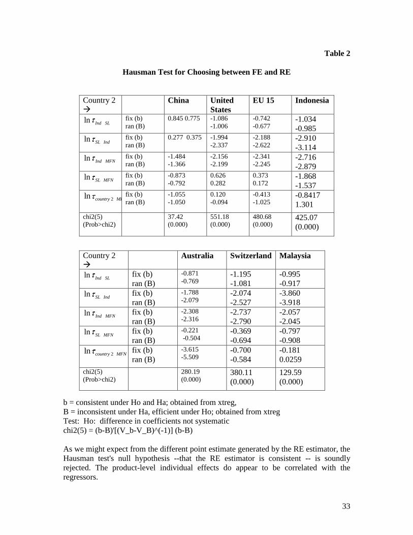
and across time. We consider these two alternatives in the Hausman test framework,
fitting both models and comparing their common coefficient estimates. As we might
28
The GTA has data for the years starting form 1998. 29
For Annex Table B, C, D and E control countries we use mirror data on imports by Sri Lanka for years
1996, 1997, 2000 and 2006 due to unavailability of Sri Lanka‘s import data as reporter to COMTRADE. 30
There may be difference of 5% to 6 % between the actual imports recorded by Sri Lanka (data not
available) and the mirror data of imports by Sri Lanka from control countries (data available). This
difference is due the fact that in COMTRADE, the imports are recorded CIF (Cost insurance and freight)
while the exports are recorded FOB (free on board). Finally, since we use the combined imports by India
(import data available for the period under study) and Sri Lanka (import data available for 1998 to 2006
and mirror data for 1996 and 1997) from control countries c‘. As India is relatively a large trading partner
in ISLFTA region, when we merge the two import data to get the combined imports by ISLFTA partners,
the difference due to CIF and FOB values for 1996 and 1997 in Sri Lankan data gets further diluted. 31
We do not use pooled OLS method to estimate our model it it i t ity x u v as it would ignore
the nature of the panel data and assumes , ,j j i t . This model will be highly restrictive and can
have heteroskedasticity across panel units or serial correlation within panel units. We may choose the
Between Estimators (BE), Fixed Effects (FE) or the Random Effects (RE) Model to estimate the panel
coefficients of our model. In the BE, the group means of y are regressed on the group means of x in a
regression of N observations. This estimator also ignores all the time variations in y and when the iu are
correlated with any of the regressors in the model, the zero-conditional-mean assumption does not hold
and the between estimator produces inconsistent results. Finally, we are left with the FE and RE models
that allows for the heterogeneity across panel units and across time. If the iu are uncorrelated with the
regressors, then we can use the RE, but if the iu are correlated with the regressors, then we use the FE
model.
20
expect from the different point estimates generated by RE estimator, the Hausman test's
null hypothesis---that the RE estimator is consistent --is soundly rejected (Table 2). The
individual effects do appear to be correlated with the regressors; hence our results are
based on the Fixed Effects Model (FE).
A summary of the results using Fixed Effects model for seven panels are given in Table
1. Interpretation of these results will essentially provide the evidence, whether ISLFTA
have been trade diverting (or trade creating). For interpreting the results, we refer to the
log-difference of combined imports of ISLFTA partners and imports of ‗country 2‘
from the control countries c‘ , given by equation (9).
Column 1 of Table 1 gives the estimates of coefficients, when we use China as our
‗country 2‘. The results shows that the sum of the coefficients on the preferential tariffs
(β1 and β2) is positive, suggesting that ISLFTA may be trade diverting for non-ISLFTA
members (control countries c‘). It shows that a 1% reduction in ISLFTA preferential
tariffs will cause 1.12 % reduction in imports by the ISLFTA countries from control
countries c‘ relative to imports by China from same control countries. All coefficients
except 2 are highly significant. The reduction in tariffs by India for Sri Lankan
products is a major contributor to creation of more trade for Sri Lanka at the expense of
control countries c‘. The MFN applied average tariff by India in 2006 is 20.79%, while
its tariff on Sri Lankan products is only 4.25% (Figure 2). On the other hand there is not
much difference between Sri Lanka‘s MFN (11.82% in 2006) and preferential applied
tariffs (9.08% in 2006) (Figure 3). This along with the fact that India is a major
importer of control country c‘ products, explains the significance of β1 and non-
significance of β2. The other coefficients i.e. β3, β4 and β5 are of expected (negative)
sign and are highly significant. A reduction in MFN tariffs by the ISLFTA countries
would increase the exports to this region from the control countries c‘. Similarly, if
country 2 (China) reduces its MFN tariff, the exports from control countries c‘ to
country 2 will increase.
In the second part of our analysis, we substitute US, EU-15, Indonesia, Australia,
Switzerland and Malaysia respectively as ‗country 2‘ thereby forming six more panels.
21
The control countries c‘ also change to countries listed in Annex II Table B, Table C,
Table A, Table D, Table E and Table A respectively. The results of regression for these
panels are reported in column 2 to 7 (Table 1). The sum of coefficients β1 and β2 is
negative in all these six cases. For example, in column 2, when we ‗country 2‘ is US,
we have sum of β1 and β2 equals –3.080 . This shows that as per estimates of our
model, when the ISLFTA countries reduce preferential tariffs by 1%, this results in an
increase of 3% in exports to the ISLFTA partners from Table B control countries c‘
compared to exports from the same control countries to US. Once again, coefficients β3
and β4 are of expected (negative) sign and highly significant, showing that a 1%
reduction in MFN tariffs by the ISLFTA countries would increase the exports from
control countries c‘ to this region by around 4% compared to exports to US from the
same countries. β5 in this case is insignificant. All the coefficients in next five panels in
Table 1 (except β5 for in case of EU15, Switzerland and Malaysia as ‗country2‘ and β4
in case of Australia and Switzerland as ‗country 2‘) are strongly significant and can be
interpreted similarly. Overall, we estimate that a 1% reduction in ISLFTA partners‘
preferential tariffs results in 2.6% to 4.9 % increase in exports from control countries c‘
to ISLFTA members compared to the exports from countries c‘ to ‗country 2‘.
As most of the coefficients of our model, including the rho and F-test statistics32
establish the significance of our model; we conclude that our model is able to assess
reasonably well the trade effects of ISLFTA.
One issue, which needs explanation is the difference in trade effects in panel 1 (trade
diversion) and six other panels (trade creation) of Table 1. Two reasons can be given to
explain this difference. First, in panel 1, ‗country 2‘ (China) is the largest exporter to
ISLFTA partners (1st to India and 3
rd largest to Sri Lanka, in 2006). When we select the
control countries c‘ with China as ‗country 2‘, we have to exclude China from the list of
control countries c‘. This affects our results by way of exclusion of almost 16% of
exports to ISLFTA partners in 2006. Second, we also have to exclude some other
countries (e.g. Hong Kong, Malaysia, Taiwan, Indonesia and Thailand) having
32
Rho, F test, F statistic and R2 have similar interpretation for all of our seven panels, we discuss them
together in detail in the Note below Table 1.

22
preferential relations with China from the list of control countries c‘. These countries
are among the top 10 exporters to ISLFTA region. These countries together with China
constitute almost 30% of exports to ISLFTA countries in 2006. This produces biased
estimates to our model by excluding a large percentage of imports by ISLFTA partners.
On the other hand, when other six countries are substituted as ‗country 2‘, we have to
exclude only 3 to 10% of total imports by ISLFTA region for estimations of equation
(9). Moreover, we find consistent and strongly significant results for our model form
column 2 to 7 in Table 1. We, therefore, tend to give more weightage to the results
obtained from panels having US, EU15 , Indonesia , Australia, Switzerland and
Malaysia as ‗country 2‘. The results show that a 1% reduction in preferential tariffs
among ISLFTA partners will increase 2.6% to 4.9% exports from control countries c‘
to ISLFTA partners as compared to the exports from control countries c‘ to ‗country 2‘ .
8 Conclusion
We have shown in this study that ISLFTA has a slight trade creation effect on non-
ISLFTA countries. The consumers in India and Sri Lanka are able to get some of the
products from the most competitive suppliers within the region; with the result they are
able to consume more goods with the same income. Apparently, this has a trade creation
effect for the non-members. We have also shown that ISLFTA is one of the few South-
South Agreements, which are working effectively. The success of ISLFTA has proved
that if the concerns of smaller economy are taken into account with more favorable
treatment, then the size differential in the economies of the FTA partners do not matter.
Immediately, after the Agreement, there has been a jump in the trade flows, which
could be attributed to the increased engagement of partner countries on products having
preferential access and due to the ‗border effect‘. We have not gone into the sector
specific analysis in this study which could be an interesting area for further research on
ISLFTA.
23
9 References
[1] Baltagi, B.H. Econometric Analysis of Panel Data, 2nd ed. New York: John
Wiley & Sons, 2001.
[2] Baldwin, R. and Rieder, R. (2007). ―A Test of Endogenous Trade Bloc
Formation Theory on EU Data‖, Journal of International Economic Studies,
Vol. 11, No.2, December 2007.
[3] Baldwin, R. (2006), ―Multilateralising Regionalism: Spaghetti Bowls as
Building Blocs on the Path to Global Free Trade‖, The World Economy,
Volume 29, Issue 11, June 2006.
[4] Baldwin, R. and Taglioni, D. (2006), ―Gravity for Dummies and Dummies for
Gravity Equations‖ NBER WP12516 , Cambridge.
[5] Baldwin, R. (2004). ―Stepping stones or building blocs? Regional and
multilateral integration‖ Forthcoming. Found at http://hei.unige.ch/~baldwin/
[6] Bhagwati, J., and A.O. Krueger. The Dangerous Drift to Preferential Trade
Agreements. Washington, DC: AEI Press, 1995.
[7] Clausing, K. ‗‗Trade Creation and Trade Diversion in the Canada–United
States Free Trade Agreement.‘‘ Canadian Journal of Economics
34(2001):677–96.
[8] DeRosa Dean A. (2007), ―The Trade Effects of Preferential Arrangements:
New Evidence from the Australia Productivity Commission‖, Peterson
Institute for International Economics, WP 07-01, January 2007.
[9] Fukao, K., T. Okuba, and R.M. Stern(2003), ‗‗An Econometric Analysis of
Trade Diversion under NAFTA.‘‘ North American Journal of Economics and
Finance 14(1), March 2003, pp. 3–24.
[10] Feridhanusetyawan T.(2005), ―Preferential Trade Agreements in the Asia-
Pacific Region‖, IMF WP/05/149, July 2005
[11] Gilbert J., Scollay R., and Bora B. (2001), ―Assessing Regional Trading
Arrangements in the Asia-Pacific‖, Policy Issues in International Trade and
Commodities Study Series No. 15, UNCTAD.
[12] Holmes T. (2005), ―What Drives Regional Trade Agreements that Work?‖,
HEI Working Paper No: 07/2005.
[13] Hsiao, C. Analysis of Panel Data. New York: Cambridge University Press,
2003.
[14] JSG (2003), India-Sri Lanka Comprehensive Economic Partnership
Agreement, Joint Study Group, October 2003, Governments of India and Sri
Lanka.
[15] Karemera, D., and W.W. Koo, ‗‗Trade Creation and Diversion Effects of the
U.S.-Canadian Free Trade Agreement.‘‘ Contemporary Economics Policy
12(1994):12–23.
24
[16] Kelegama, S. and Mukherji I.N. (2007), ―India-Sri Lanka Bilateral Free Trade
Agreement: Six Years Performance and Beyond‖, RIS DP# 119, February
2007, Research and Information System for Developing Countries, New
Delhi.
[17] Kelegama, S. , Mukherji I.N. and Jayawardhana T. (2002), ―Indo-Sri Lanka
Free Trade Agreement: An Assesment of Potential and Impact‖, SANEI
[18] Kruger, A.O. ‗‗Free Trade Agreements versus Customs Unions.‘‘ Journal of
Development Economics 54(1997):169–87.
[19] Panagariya, A. ‗‗Preferential Trade Liberalization: The Traditional Theory and
New Developments.‘‘ Journal of Economic Literature 38(2000):287–331.
[20] Susanto, Parr Rosson, and Adcock (2007), ―Trade Creation and Trade
Diversion in the North American Free Trade Agreement: The Case of the
Agricultural Sector‖, Journal of Agricultural and Applied Economics,
39,1(April 2007): pp.121–134.
[21] Romalis J. (2005), ―NAFTA‘s and CUSFTA‘s Impact on International Trade‖,
NBER WP11059, Cambridge.
[22] UNDP (2005), ―The Great Maze, Regional and Bilateral Free Trade
Agreements in Asia‖ Discussion Paper, Asia-Pacific Trade and Investment
Initiative, UNDP Regional Centre, Colombo, September 2005.
[23] USITC (2003) , ―Chapter 6: The Impact of NAFTA Preferences on U.S.-
Mexican Trade: A Sectoral Approach‖, The Impact of Trade Agreements,
United States International Trade Commission, August 2003.
[24] Viner, J. The Customs Union Issue. New York: Carnegie Endowment for
International Peace, 1950.
[25] Wooldridge, J.M. Econometric Analysis of Cross Section and Panel Data.
Cambridge, MA: MIT Press, 2002.
[26] World Bank (2005), ―Global Economic Prospects 2005: Trade, Regionalism
and Development‖, November 2004, Washington.
25
Figure 1 : Free Trade Agreements in Asia –Cumulative Status (as of December,
2007)
Data Source: ADB, Manila
Figure by Author
Note: The numbers include -- Proposed, Under Negotiation, Signed and Under Implementation Free
Trade Agreements.
0
50
100
150
200
2501
97
5
19
80
19
82
19
89
19
92
19
94
19
96
19
98
20
00
20
02
20
04
20
06
Nu
mb
ers
Year
FTAs

26
Figure 2: India’s Average Applied MFN and Preferential Tariffs
Data Source: WITS, World Bank
Figure by Author
Figure 3: Sri Lanka’s Average Applied MFN and Preferential Tariffs
Data Source: WITS, World Bank
Figure by Author
0.00
5.00
10.00
15.00
20.00
25.00
30.00
35.00
40.00
45.00
19
96
19
97
19
98
19
99
20
00
20
01
20
02
20
03
20
04
20
05
20
06
Ad
-val
ore
m T
arif
f
Year
MFN Avg
for SL Avg
0.00
5.00
10.00
15.00
20.00
25.00
19
96
19
97
19
98
19
99
20
00
20
01
20
02
20
03
20
04
20
05
20
06
Ad
val
ore
m T
arif
f
Year
MFN Average
for India Average
27
Figure 4 : Growth in India’s Imports from Sri Lanka and Rest of the World (1996
to 2006, index 1996=100)
Data Source: COMTRADE
Figure by Author
Figure 5 : Growth in Sri Lanka’s Imports from India and Rest of the World (1996
to 2006, index 1996=100)
Data Source: COMTRADE
Figure by Author
-200
0
200
400
600
800
1000
1200
1400
19
96
19
97
19
98
19
99
20
00
20
01
20
02
20
03
20
04
20
05
20
06
% G
row
th (
19
96
bas
e)
Year
Sri Lanka
ROW
-50
0
50
100
150
200
250
19
96
19
97
19
98
19
99
20
00
20
01
20
02
20
03
20
04
20
05
20
06
% G
row
th (
19
96
bas
e)
Year
IND
ROW

28
Figure 6: Share of Sri Lankan Goods to India and China’s Total Imports
Data Source: COMTRADE
Figure by Author
Figure 7: Share of Some Major Exporters and Sri Lanka
to India’s Total Imports
Data Source: COMTRADE
Figure by Author
0.000
0.001
0.002
0.003
0.004
0.005
0.006
0.007
0.000
0.050
0.100
0.150
0.200
0.250
0.300
0.350
0.400
0.450
19
96
19
97
19
98
19
99
20
00
20
01
20
02
20
03
20
04
20
05
20
06
% s
har
e in
Ch
ina
% s
har
e in
Ind
ia
Year
SLs share in India Imp
SLs share in China Imp
0.00
0.05
0.10
0.15
0.20
0.25
0.30
0.35
0.40
0.45
0.00
5.00
10.00
15.00
20.00
25.00
30.00
19
96
19
97
19
98
19
99
20
00
20
01
20
02
20
03
20
04
20
05
20
06
SL P
erc
en
t
Pe
rce
nt
Year
CHN
EU 15
USA
SL

29
Figure 8: Sri Lanka’s Share of India’s Total Imports on Items
Under Different List of ISLFTA
Data Source: COMTRADE
Figure by Author
0.000
0.200
0.400
0.600
0.800
1.000
1.200
1.400
1.600
19
96
19
97
19
98
19
99
20
00
20
01
20
02
20
03
20
04
20
05
20
06
Year
Negative List: % SL Imp
Positive List: % SL Imp
Residual List: % SL Imp
Total Imports: % SL Imp

30
Table 1
Trade Diversion/Creation Effects from India Sri Lanka FTA
*** shows coefficient is significant at 1% level.
** shows coefficient is significant at 5% level.
* shows coefficient is significant at 10% level.
N= number of observations, n= number of groups, k= number of dependent variables.
For explanation of various entries in the above table, refer note on the next page.
lm# 1 2 3 4 5 6 7
Trade
Diversion/
Creation
Diversion Creation Creation Creation Creation Creation Creation
1 2( ) 1.122
(0.000)
-3.080
(0.000)
-2.930
(0.000)
-3.944
(0.000)
-2.660
(0.000)
-3.269
(0.000)
-4.855
(0.000)
ln Ind SL 0.845
(0.079)
10.74***
-1.086
(0.065)
-16.64***
-0.742
(0.063)
-11.78***
-1.034
(0.086)
-11.98***
-0.871
(0.071)
-12.22***
-1.195
(0.084)
-14.26***
-0.995
(.075)
-13.34***
ln SL Ind 0.277
(0.296)
0.94
-1.994
(0.250)
-7.96***
-2.188
(0.243)
-9.01***
-2.910
(0.338)
-8.60***
-1.789
(0.274)
-6.53***
-2.074
(0.314)
-6.60***
-3.860
(0.286)
-13.48***
ln Ind MFN -1.484
(0.136)
-10.92***
-2.156
(0.113)
-19.02***
-2.341
(0.110)
-21.28***
-2.716
(0.153)
-17.77***
-2.309
(0.127)
-18.14***
-2.737
(0.147)
-18.64***
-2.057
(0.132)
-15.64***
ln SL MFN -0.873
(0.280)
-3.11***
0.626
(0.238)
2.62***
0.374
(0.233)
1.60*
-1.868
(0.319)
-5.85***
-0.221
(0.260)
-0.85
-0.369
(0.300)
-1.23
-0.797
(0.274)
-2.91***
2ln country MFN
-1.055
(0.199)
-5.29***
0.121
(0.618)
0.20
-0.414
(0.292)
-1.42
-0.842
(0.364)
-2.31**
-3.615
(0.492)
-7.34***
-0.700
(0.444)
-1.58
-0.181
(0.163)
-1.11
_constant -1.340
(0.031)
-42.76***
-2.330
(0.030)
-76.50***
-2.894
(0.027)
-108.60***
1.916
(0.037)
51.47***
0.537
(0.030)
18.06***
2.030
(0.035)
58.08***
0.887
(0.031)
28.54***
Country 2 China USA EU15 Indonesia Australia Switzer-
land
Malaysia
Control
Countries
Table A Table B Table C Table A Table D Table E Table A
Number of
Observations
49721 49775 50637 48504 48652 45702 46661
Number of
products
4987 5013 5049 4998 4942 4916 4935
R-sq within 0.005 0.058 0.054 0.066 0.057 0.059 0.074
rho (variation
due to ui )
0.678 0.812 0.784 0.626 0.783 0.802 0.677
F(n-1, N-n-k)
F test that all ui =0
17.25
(0.000)
34.58
(0.000)
29.29
(0.000)
13.29
(0.000)
28.35
(0.000)
29.88
(0.000)
16.36
(0.000)
F (k, N-n-k)
significance of
the model
43.66
(0.000)
550.31
(0.000)
524.84
(0.000)
618.55
(0.000)
523.58
(0.000)
514.89
(0.000)
666.16
(0.000)

31
Note on Table 1:
i) # lm (the dependent variable)
= log (Import in India +Sri Lanka form the control countries) – log (Import in ‗country
2‘ form the control countries c‘) for each HS 6 digit product for each year (1996 to
2006), i.e. log-difference between FTA partners‘ combined imports and ‗country 2‘
import form the Control Countries.
ii) The Control Countries are selected based on ‗country 2‘ chosen for analysis. The
Control Countries are shown in Table A, B, C, D and E. Control Countries include all
the countries reporting the data to COMTRADE, minus India, Sri Lanka, ‗country 2‘
and other countries having preferential trade arrangement with ‗country 2‘. For
example, in case of China, the Annex II Table A Control Countries include--- 180
COMTRADE countries minus China, India, Sri Lanka, Hong Kong China, Macao
China, and ASEAN countries (Brunei Darussalam, Cambodia, Indonesia, Laos,
Malaysia, Myanmar, Philippines, Singapore, Thailand, Vietnam) i.e. 165 countries.
iii) The dependent variable (lm) is regressed on tariffs on 6 digit products of HS 1996
classification applied by
(a) India on Sri Lankan imports—preferential tariffs,
(b) Sri Lanka on Indian imports—preferential tariffs,
(c) India on imports from control countries—MFN tariffs,
(d) Sri Lanka on imports from control countries—MFN tariffs,
(e) the ‗country 2‘ on imports form control countries—MFN tariffs.
iv) We use simple average of applied ad valorem tariffs for all products at 6 digit level.
For the products with specific duties, we calculate the ad-valorem equivalents form
WITS by using methodology adopted in NAMA negotiations at WTO.
v) The Import of products is measured on a CIF basis, the units used are $‘000 per
year.
vi) We use Product Specific Effects and Time Specific Effects in our model and use
Panel Data Fixed Effects methodology for all our estimations.
viii) The first row of the above table reports Trade Diversion or Trade Creation effects
based on sign of the sum of coefficients ( 1 2 ) of preferential tariffs charged by FTA
partners . The second row reports the sum of the coefficients 1 2 (the first two
coefficients reported below). The p- value is based on a F-test that the coefficients on
the regressors are all jointly zero. The p-values are reported in the brackets below
1 2 . A positive significant sum of the coefficients 1 2 , indicate Trade Diversion
as a result of the ISLFTA. A negative significant sum of the two coefficients indicates
Trade Creation Effects resulting from the ISLFTA.
ix) The figures reported below the tariff coefficients in the brackets are the standard
errors (se). The t-values are shown below the se in each cell of the table. The significant
t-values are marked by asterisks at acceptable level of significance.
x) _cons : Stata fits a model, in which the ui (i.e. individual specific fixed effects Dz)
are taken as deviations from one constant term, displayed as _cons.
x) The number of observations with different ‗country 2‘ varies due the change in
products imported by these countries from the control countries. In addition, the
difference also arises because; we have dropped the observations with extremely high
tariffs (more than 65%).

32
xi) R2 (within) is reported in the fourth last row. Stata command xtreg, fe obtains its
estimates by performing OLS on transformed model, so the R2 reported do not have all
the properties of the OLS R2 .
xi) rho values estimate that 67 % to 81% of variation in log-difference between
combined imports of ISLFTA partners and imports of ‗country 2‘ from the control
countries c‘ (i.e. dependent variable ,lm) is due to the product specific differences ui
(i.e. Dz) .
xii) F (n-1, N-n-k) : F test provides a test of the null hypothesis Ho that all ui =0 . In
other words, we wish to test whether the individual specific heterogeneity of ui is
necessary i.e. are there distinguishable intercept terms across units? A rejection of this
Ho indicates that pooled OLS would produce inconsistent estimates.
xiii) F (k, N-n-k): F statistics to test the null Ho that the coefficients on the regressors
(dependent variables) are jointly zero i.e. whether our model is overall significant. A
rejection of Ho implies that our model is overall significant. The F-statistic in all the
cases shows high significance level for our model as a tool to explain the trade effects
of the FTA.
33
Table 2
Hausman Test for Choosing between FE and RE
Country 2
China United
States
EU 15 Indonesia
ln Ind SL fix (b)
ran (B)
0.845 0.775 -1.086
-1.006
-0.742
-0.677 -1.034
-0.985
ln SL Ind fix (b)
ran (B)
0.277 0.375 -1.994
-2.337
-2.188
-2.622 -2.910
-3.114
ln Ind MFN fix (b)
ran (B)
-1.484
-1.366
-2.156
-2.199
-2.341
-2.245 -2.716
-2.879
ln SL MFN fix (b)
ran (B)
-0.873
-0.792
0.626
0.282
0.373
0.172 -1.868
-1.537
2ln country MFN
fix (b)
ran (B)
-1.055
-1.050
0.120
-0.094
-0.413
-1.025 -0.8417
1.301
chi2(5)
(Prob>chi2)
37.42
(0.000)
551.18
(0.000)
480.68
(0.000) 425.07
(0.000)
Country 2
Australia Switzerland Malaysia
ln Ind SL fix (b)
ran (B)
-0.871
-0.769 -1.195
-1.081
-0.995
-0.917
ln SL Ind fix (b)
ran (B)
-1.788
-2.079 -2.074
-2.527
-3.860
-3.918
ln Ind MFN fix (b)
ran (B)
-2.308
-2.316 -2.737
-2.790
-2.057
-2.045
ln SL MFN fix (b)
ran (B)
-0.221
-0.504 -0.369
-0.694
-0.797
-0.908
2ln country MFN
fix (b)
ran (B)
-3.615
-5.509 -0.700
-0.584
-0.181
0.0259
chi2(5)
(Prob>chi2)
280.19
(0.000) 380.11
(0.000)
129.59
(0.000)
b = consistent under Ho and Ha; obtained from xtreg,
B = inconsistent under Ha, efficient under Ho; obtained from xtreg
Test: Ho: difference in coefficients not systematic
chi2(5) = (b-B)'[(V_b-V_B)^(-1)] (b-B)
As we might expect from the different point estimate generated by the RE estimator, the
Hausman test's null hypothesis --that the RE estimator is consistent -- is soundly
rejected. The product-level individual effects do appear to be correlated with the
regressors.

34
Annex I
ISLFTA – Commitment of Member Countries in Brief33
Mutual phased tariff concessions on 5112 items on 6 digits (HS1996) have been agreed.
An eight year time-table was specified for phasing out tariffs on all tariff lines, except
the items on negative list of each country.
India’s commitment:
i) Duty free access to 1,351 items upon entry into force of the Agreement
in March 2000.
ii) Duty concession of 25% on 528 items in HS chapters 51 to 56, 58 to 60
and 63.
iii) Margin of preference of 50% on the remaining items of 2,799 increased
to 100% in two stages in March 2003
iv) Duty concession of 50% on 233 tariff items of ready made garments and
5 tariff items of tea. This concession is under a tariff rate quota (TRQ)34
of 15 million kg on tea and of 8 million pieces on garments.
v) Negative List of 429 items from rubber, paper, plastic, coconuts,
alcoholic beverages and textile sector
Sri Lanka’s commitment:
i) Duty free access to 319 items upon entry into force of the Agreement in
March 2000.
ii) Margin of preference of 50% on 839 items deepened to 70%, 90% and
100% at the end of 2001, 2002 and 2003 respectively
iii) For 2,724 items, the tariff brought down to
35% by March 2003
70% by March 2006
100% by March 2008
iv) Negative List of 1180 items from agriculture, automobile, electrical
machinery, aluminum, copper, Iron & Steel, rubber, paper and plastic .
Rules of Origin:
i) the domestic value addition should be 35%; if the raw material /inputs
are sourced from one member by the other, the value addition is reduced
to 25% within the overall limit of 35%.
ii) inputs to undergo substantial transformation at 4 digit level of customs
Harmonized Code; and
iii) a list of operations such as simple packing, cutting and assembly, have
been defined which do not qualify for preferential market access.
33
For complete details, the interested reader is referred to Sri Lanka‘s Department of Commerce website.
http://www.doc.gov.lk/web/indusrilanka_freetrade.php. 34
A tariff rate quota is a quantity which can be imported at a certain duty. Any quantity above that
amount is subject to a higher tariff.
35
Annex II
Control Countries
Country 2 Table List of Control Countries Remarks
China Table A
The 180 COMTRADE countries minus
China, India, Sri Lanka, minus Hong
Kong China, Macao China, and ASEAN
countries (Brunei Darussalam,
Cambodia, Indonesia, Laos, Malaysia,
Myanmar, Philippines, Singapore,
Thailand, Vietnam).
165 Countries with no
substantial change in
preferential trade relations
with China
United States Table B
The 180 COMTRADE countries minus
United States, India, Sri Lanka, minus
Australia, Canada, Chile, Israel, Jordan,
Mexico and Singapore.
170 Countries with no
substantial change in
preferential trade relations
with the United States
European
Union-15
Table C The 180 COMTRADE countries minus
EU-15, India, Sri Lanka, minus Algeria,
Andorra, Chile, Croatia, Egypt, Faroe
Island, Iceland, Israel, Jordan, Lebanon,
Mexico, Morocco, Norway, South
Africa, Syrian Arab Republic,
Switzerland, Tunisia and Turkey.
144 Countries with no
substantial change in
preferential trade relations
with the EU-15
Indonesia Table A
The 180 COMTRADE countries minus
China, India, Sri Lanka, minus Hong
Kong China, Macao China, and ASEAN
countries (Brunei Darussalam,
Cambodia, Indonesia, Laos, Malaysia,
Myanmar, Philippines, Singapore,
Thailand, Vietnam).
165 Countries with no
substantial change in
preferential trade relations
with Indonesia
Australia Table D The 180 COMTRADE countries minus
Australia, India, Sri Lanka, minus New
Zealand, Singapore, Thailand and United
States.
173 Countries with no
substantial change in
preferential trade relations
with Australia
Switzerland Table E The 180 COMTRADE countries minus
Switzerland, India, Sri Lanka, minus EU-
15 (Austria, Belgium, Denmark, Finland,
France, Germany, Greece, Ireland, Italy,
Luxembourg, Netherlands, Portugal,
Spain, Sweden and United Kingdom) ,
Iceland, Liechtenstein, Norway (EFTA
countries) and Faroe Islands.
159 Countries with no
substantial change in
preferential trade relations
with Switzerland
Malaysia Table A
The 180 COMTRADE countries minus
China, India, Sri Lanka, minus Hong
Kong China, Macao China, and ASEAN
countries (Brunei Darussalam,
Cambodia, Indonesia, Laos, Malaysia,
Myanmar, Philippines, Singapore,
Thailand, Vietnam).
165 Countries with no
substantial change in
preferential trade relations
with Malaysia
Note: The above table gives the list of control countries in brief. For transparency, the complete list can
be obtained on request by sending an email to me at [email protected] .