analysis of image noise due to position errors in laser writers

Analysis of image noise due to position errorsin laser writers

Peter D. Burns, Majid Rabbani, and Lawrence A. Ray

For raster-written images, the modulated laser exposing beam is scanned across the photosensitive material ina line-by-line configuration. Image noise can be introduced by the writer directly, for example, by thegranularity of the photosensitive materials and indirectly, for example, by beam position errors. For analysisof the effect of position errors they must first be related to their resultant exposure fluctuations. Here,position errors are addressed via models of image writing that include several spot/pixel writing schemes.Three types of image noise due to page-scan position error are examined. The effect of low-frequencyposition errors is described. Exposure fluctuations due to broadband stochastic errors are then addressed.For laser writers using a rotating polygon for beam deflection, the effect of stochastic facet-angle errors isrepeated down the image; this results in periodic exposure fluctuations and is the third type of image noiseanalyzed. Expressions are given for the mean and variance of the exposure error in terms of the statistics ofthe position error, writing spot profile, and raster sampling distance. The analytical models are thencompared with the results of an image simulation calculation. In this way, the exposure error fluctuations aredescribed by their noise power spectra as functions of spatial frequency. After consideration of the sensitom-etry of the hardcopy recording materials, the exposure errors are then related to the corresponding outputdensity fluctuations.

1. Introduction

Most laser image writers scan the laser light sourceacross the photosensitive material in a line-by-line, orraster, format, which is well suited to both continuoustone and text imaging.1 The exposing beam is de-flected across the photosensitive material, while thematerials are moved incrementally in the orthogonaldirection, for each raster line. The beam intensity ismodulated at discrete intervals corresponding to theintended optical density of each pixel in the final im-age. Reference 1 gives more details of various deflec-tion schemes. This process can be thought of as aconversion of the image from a 1-D sampled digitalsequence to a 2-D continuous representation.

The design of a laser writer places limitations on thisconversion from discrete to continuous form that in-troduce error or image noise. Consider, for example,the case where the discrete signal is merely a sampledversion of an input optical image. The corresponding

The authors are with Eastman Kodak Company, Research Lab-oratories, Rochester, New York 14650.

Received 6 December 1985.0003-6936/86/132158-11$02.00/0.© 1986 Optical Society of America.

written image will contain fluctuations attributable tothe finite number of levels (bits) used for the discretesampled image. Other sources of image noise intro-duced by the image writer are stochastic variations inthe laser beam intensity, granularity of the photosensi-tive material, and beam position (or velocity) errors.The first two noise sources can be analyzed by consid-ering the signal and noise transfer during modulationand image writing. Position errors, however, mustfirst be related to their resultant output exposure fluc-tuations. Our focus is on errors that occur in the slowor page scan direction causing the line pitch to vary.

Since the written exposure image is dependent onthe repeated raster scanning of the laser, errors in theline position degrade image quality. This occurs withthe introduction of 1-D banding and streak artifactswhich will be most evident in the constant or low-contrast image areas. Often the design goal is to setposition error tolerance values so that no banding arti-facts are visible under normal viewing conditions.These tolerance levels vary due to several factors, e.g.,pixel writing configuration, contrast of the recordingmaterial, and nature of the position errors. Besten-reiner et al.

2 have investigated the effect of periodicline position errors on the reproduction of halftone andcontinuous-tone recording processes. They foundthat viewers could detect the presence of low-frequen-cy periodic image fluctuations due to fractional posi-tion errors of 1%. The sensitivity of human vision to

2158 APPLIED OPTICS / Vol. 25, No. 13 / 1 July 1986

(a)Exposure

Y 2Y 3Y

Distance

Input signal

( b) / \ Rastering

Modulus signal

Reconstructionfunction

l/Y

Spatial frequency

Fig. 1. (a) Effect of overlapping exposure beams corresponding to aconstant input signal. (b) Frequency domain representation ofabove. The constant input is aliased at 1/Y, since the reconstruction

function is not bandlimited.

where the zero-frequency mean signal is aliased at thesampling frequency, as shown in Fig. 1(b). For a con-stant input exposure I, the written output exposure is

C(x) = I + 2IR(1/Y) cos(2irx/Y), (1)

where Y is the constant line-pitch distance, and R(f) isthe Fourier transform of the spot profile. Here weassume that the rastering components at multiples ofthe sampling frequency are negligible. Note that thisperiodic fluctuation has a high spatial frequency, twicethe Nyquist frequency, and is usually not'in a region ofhigh visual sensitivity. We address it here recognizingthat this component is present in a written image in theabsence of position errors. Fluctuations in images dueto position errors will be considered separately fromfluctuations due to other causes.

For many systems the reconstruction function Rlimits signal modulation and, therefore, is equal to theMTF. However, since other transfer functions (fil-ters) can be operating on the signal, we will not refer toR as the system MTF. The output exposure is thedesired constant plus a raster cosine signal. The aver-age exposure C can be written as a function of beamvelocity or line pitch:

C(ergs/cm 2S) = J(ergs/cm s2)

s(cm/s)

C(ergs/cm 2 S) = K(ergs/cm s)(2)

these artifacts, however, will strongly depend on thespatial frequency of their components.3

Laser writers have several sources of position errors,and rarely do current designs meet such stringenttolerances. Values of 5-20% are typical. Kessler andShack4 describe measurement of several sources forlaser printers using a polygon spinner for beam deflec-tion. Scanning accuracy for galvanometer deflectorshas been addressed by Brosens.5 Many applicationsrequire a secondary correcting deflector to compensatefor systematic line-position errors.26 Although theoriginal uncompensated position errors may be knownor periodic, the residual errors after compensation willoften contain stochastic components.

To date, no general analysis of image noise due toraster-line position errors is available. This work ad-dresses the effect of periodic and stochastic positionerrors and explicitly includes the effect of the modulat-ed laser beam shape. The objective is to provide phys-ical understanding of the effect on the image that canbe related to other imaging characteristics of the laserprinter, such as mean density, contrast, and MTF.

II. Low-Frequency Position Errors

We start by assuming that we are printing a uniformimage area at some signal level with no position errorsas in Fig. 1(a). When images are sampled and recon-structed, they are subject to both filtering (blurring)and aliasing.7 8 Rastering is an example of aliasing

where s is the fast scan beam velocity, and J, K areconstant scale factors dependent on the exposuresource and optics.

Consider the effect of low-amplitude low-frequency(temporal and spatial) errors that cause the line pitchto vary across the image. Now Y can be a randomvariable. Combining Eqs. (1) and (2),

- =K 2KCW =x) + R(1/Y) cos(27rx/!'),

y y (3)

where the tilde indicates a random variable. Equation(3) shows that both the mean exposure and periodicraster ripple will be functions of the varying line pitch.Ignoring the second term of Eq. (3), the variation inexposure due to low-frequency stochastic position er-ror can be expressed as

crc cK y_- = Y (4)

where C and Y are now mean values. The same resultholds for low-frequency sinusoidal position error dueto, for example, stage flutter:

AC AYC Y

(5)

where AY is the sinusoidal position error. Equations(4) and (5) show that the result of low-frequency ran-dom or sinusoidal position errors is a correspondingproportional error in output exposure.

1 July 1986 / Vol. 25, No. 13 / APPLIED OPTICS 2159

111. Random Line-Position Errors

We now turn to the analysis of random line-positionerrors. Here we assume that the errors in raster posi-tions are independent, so structured errors such asthose generated from a rotating polygon or periodicvibration are excluded. The natural shape of the laserspot is a Gaussian profile; however, by using masks theshape of the spot can be altered. The work of Lee,9Ray,'0 and Sullivan" describes this process and itsmotivation. The pyramid, or linear interpolator (LI),profile is important because of both reduced signalaliasing and no raster ripple component. Consequent-ly, we consider the effect of a chosen beam shape onexposure fluctuations because of the random positionerrors.

Model

Our model as above is one-dimensional, since theerrors are assumed to be mislocations of the raster linesand not individual pixels. For a constant digital sig-nal, the ideal reconstructed exposure is

C(x) = E si(x),.A=_@

(6)

where S(x) is the spot profile in the slow scan direction.The corrupted noisy exposure because of position er-rors is

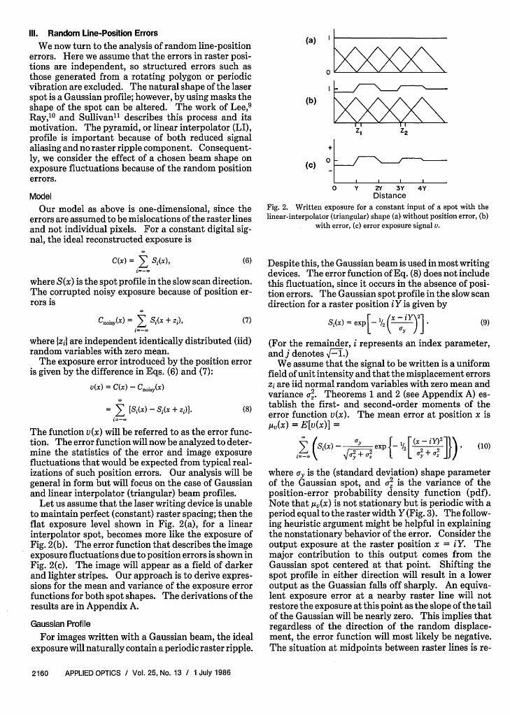
(a)

0

(b)

(C) -

IIZI

IIZ2

I I I I

0 Y 2Y 3YDistance

4Y

Fig. 2. Written exposure for a constant input of a spot with thelinear-interpolator (triangular) shape (a) without position error, (b)

with error, (c) error exposure signal v.

Despite this, the Gaussian beam is used in most writingdevices. The error function of Eq. (8) does not includethis fluctuation, since it occurs in the absence of posi-tion errors. The Gaussian spot profile in the slow scandirection for a raster position iY is given by

Cnoisy(x) = E S(x + Zi),,= X

(7)

where zi} are independent identically distributed (iid)random variables with zero mean.

The exposure error introduced by the position erroris given by the difference in Eqs. (6) and (7):

V(X) = C(x) - Cnoisy(X)

= E [Si(x) - Si(x + zi)]. (8)

The function v(x) will be referred to as the error func-tion. The error function will now be analyzed to deter-mine the statistics of the error and image exposurefluctuations that would be expected from typical real-izations of such position errors. Our analysis will begeneral in form but will focus on the case of Gaussianand linear interpolator (triangular) beam profiles.

Let us assume that the laser writing device is unableto maintain perfect (constant) raster spacing; then theflat exposure level shown in Fig. 2(a), for a linearinterpolator spot, becomes more like the exposure ofFig. 2(b). The error function that describes the imageexposure fluctuations due to position errors is shown inFig. 2(c). The image will appear as a field of darkerand lighter stripes. Our approach is to derive expres-sions for the mean and variance of the exposure errorfunctions for both spot shapes. The derivations of theresults are in Appendix A.

Gaussian Profile

For images written with a Gaussian beam, the idealexposure will naturally contain a periodic raster ripple.

Si(x) = exp 1/2 ( Y) 2] (9)

(For the remainder, i represents an index parameter,and j denotes SET.)

We assume that the signal to be written is a uniformfield of unit intensity and that the misplacement errorszi are iid normal random variables with zero mean andvariance a. Theorems 1 and 2 (see Appendix A) es-tablish the first- and second-order moments of theerror function v(x). The mean error at position x isAv(x) = E[v(x)] =

i ( - Y exp - E(X -jy) 2

/2 1 r c 2 I iL Y + Z

(10)

where cy is the (standard deviation) shape parameterof the Gaussian spot, and a 2 is the variance of theposition-error probability density function (pdf).Note that gv(x) is not stationary but is periodic with aperiod equal to the raster width Y (Fig. 3). The follow-ing heuristic argument might be helpful in explainingthe nonstationary behavior of the error. Consider theoutput exposure at the raster position x = iY. Themajor contribution to this output comes from theGaussian spot centered at that point. Shifting thespot profile in either direction will result in a loweroutput as the Guassian falls off sharply. An equiva-lent exposure error at a nearby raster line will notrestore the exposure at this point as the slope of the tailof the Gaussian will be nearly zero. This implies thatregardless of the direction of the random displace-ment, the error function will most likely be negative.The situation at midpoints between raster lines is re-


.010

.006

0

C

Co

Co

.002

-.002

-.006 a/ ]

-. 010 I I I I

0.00 0.50 1.00 1.50Rasters

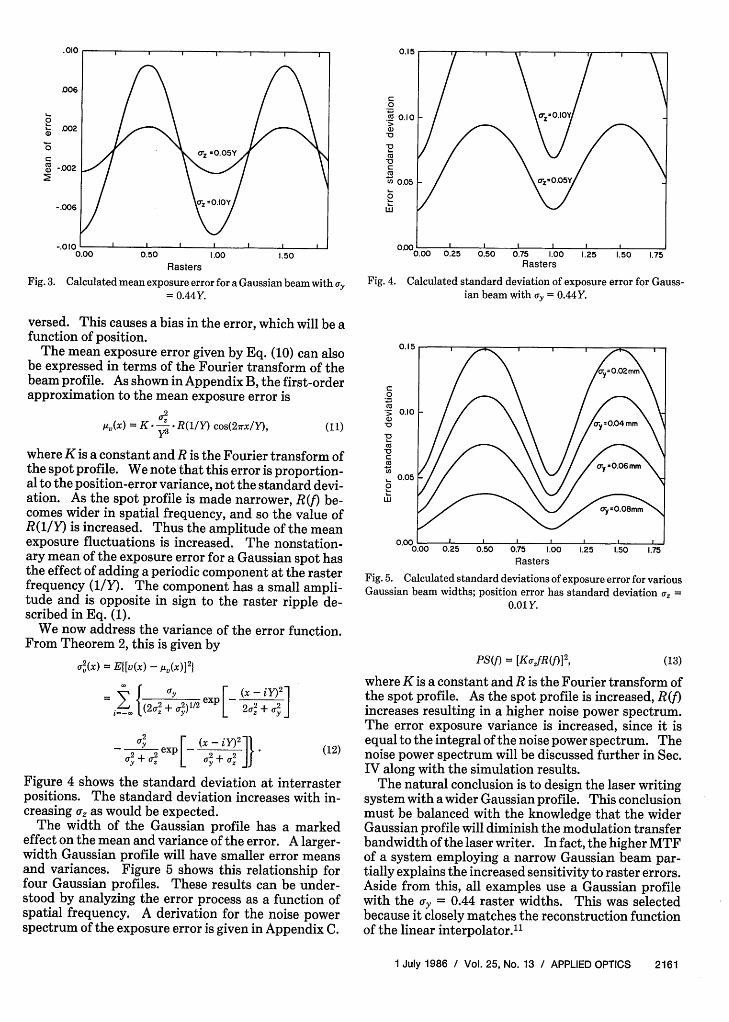
Fig. 3. Calculated mean exposure error for a Gaussian beam with a,= 0.44Y.

versed. This causes a bias in the error, which will be afunction of position.

The mean exposure error given by Eq. (10) can alsobe expressed in terms of the Fourier transform of thebeam profile. As shown in Appendix B, the first-orderapproximation to the mean exposure error is

,2

A,(x) = K R(1/Y) cos(2irx/Y), (11)

where K is a constant and R is the Fourier transform ofthe spot profile. We note that this error is proportion-al to the position-error variance, not the standard devi-ation. As the spot profile is made narrower, R(f) be-comes wider in spatial frequency, and so the value ofR(1/Y) is increased. Thus the amplitude of the meanexposure fluctuations is increased. The nonstation-ary mean of the exposure error for a Gaussian spot hasthe effect of adding a periodic component at the rasterfrequency (1/Y). The component has a small ampli-tude and is opposite in sign to the raster ripple de-scribed in Eq. (1).

We now address the variance of the error function.From Theorem 2, this is given by

(Yu(x) = El[v(x) - !_t(x)]21

-O cr [ (x (12(X)-iy2cr UY2 x -exp__-

X (12)

Figure 4 shows the standard deviation at interrasterpositions. The standard deviation increases with in-creasing a, as would be expected.

The width of the Gaussian profile has a markedeffect on the mean and variance of the error. A larger-width Gaussian profile will have smaller error meansand variances. Figure 5 shows this relationship forfour Gaussian profiles. These results can be under-stood by analyzing the error process as a function ofspatial frequency. A derivation for the noise powerspectrum of the exposure error is given in Appendix C.

C0 iD010 1 / <~~~~010.10~ ~~~~~~~0.O

C:

0.05

0.00 I l l 0.00 0.25 0.50 0.75 1.00 1.25 1.50 1.75Rasters

Fig. 4. Calculated standard deviation of exposure error for Gauss-ian beam with a, = 0.44Y.

0.15

C0

Co 0.00

-o o-..0.04mm

V~~~~~~~~

0.05~ ~ ~~001Y

PS(f) = [KorjR(f)2, (13)

where K is a constant and R is the Fourier transform ofthe spot profile. As the spot profile is increased, R(f)increases resulting in a higher noise power spectrum.The error exposure variance is increased, since it isequal to the integral of the noise power spectrum. Thenoise power spectrum will be discussed further in Sec.IV along with the simulation results.

The natural conclusion is to design the laser writingsystem with a wider Gaussian profile. This conclusionmust be balanced with the knowledge that the widerGaussian profile will diminish the modulation transferbandwidth of the laser writer. In fact, the higher MTFof a system employing a narrow Gaussian beam par-tially explains the increased sensitivity to raster errors.Aside from this, all examples use a Gaussian profilewith the y = 0.44 raster widths. This was selectedbecause it closely matches the reconstruction functionof the linear interpolator."


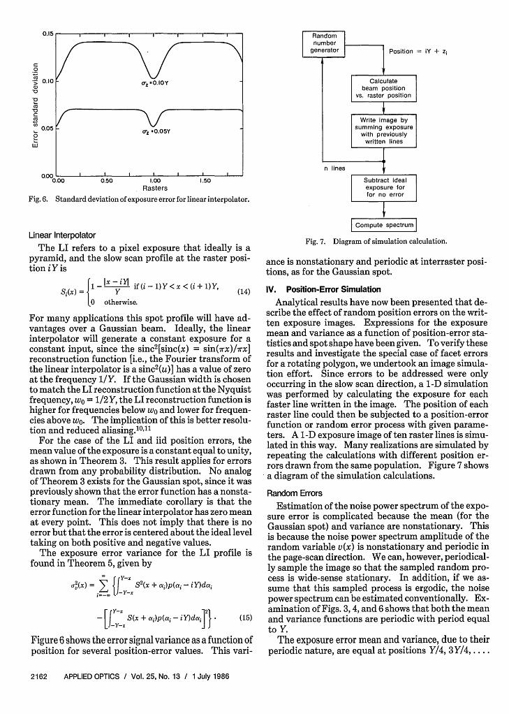
Randomnumber

generator Position =

Calculatebeam position

vs. raster position

Write image bysumming exposure

with previouslywritten lines I

n lines

0.00 0.50 1.00 1.50Rasters

Fig. 6. Standard deviation of exposure error for linear interpolator.

iY + i

Linear Interpolator

The LI refers to a pixel exposure that ideally is apyramid, and the slow scan profile at the raster posi-tion iY is

S(x) = i1 - if(i-1)Y<x <(i+1)Y,

0 otherwise.

(14)

For many applications this spot profile will have ad-vantages over a Gaussian beam. Ideally, the linearinterpolator will generate a constant exposure for aconstant input, since the sinc2[sinc(x) = sin(7rx)/rx]reconstruction function [i.e., the Fourier transform ofthe linear interpolator is a sinc2 (u)] has a value of zeroat the frequency 1/Y. If the Gaussian width is chosento match the LI reconstruction function at the Nyquistfrequency, wo = 1/2Y, the LI reconstruction function ishigher for frequencies below wo and lower for frequen-cies above wo. The implication of this is better resolu-tion and reduced aliasing.10"'1

For the case of the LI and iid position errors, themean value of the exposure is a constant equal to unity,as shown in Theorem 3. This result applies for errorsdrawn from any probability distribution. No analogof Theorem 3 exists for the Gaussian spot, since it waspreviously shown that the error function has a nonsta-tionary mean. The immediate corollary is that theerror function for the linear interpolator has zero meanat every point. This does not imply that there is noerror but that the error is centered about the ideal leveltaking on both positive and negative values.

The exposure error variance for the LI profile isfound in Theorem 5, given by

UrV(X) = X, {i S2(x + ai)p(a - iY)dMai

-[J S(x + ai)p(ai - iY)dai} * (15)

Figure 6 shows the error signal variance as a function ofposition for several position-error values. This vari-

Compute spectrum |

Fig. 7. Diagram of simulation calculation.

ance is nonstationary and periodic at interraster posi-tions, as for the Gaussian spot.

IV. Position-Error Simulation

Analytical results have now been presented that de-scribe the effect of random position errors on the writ-ten exposure images. Expressions for the exposuremean and variance as a function of position-error sta-tistics and spot shape have been given. To verify theseresults and investigate the special case of facet errorsfor a rotating polygon, we undertook an image simula-tion effort. Since errors to be addressed were onlyoccurring in the slow scan direction, a 1-D simulationwas performed by calculating the exposure for eachfaster line written in the image. The position of eachraster line could then be subjected to a position-errorfunction or random error process with given parame-ters. A 1-D exposure image of ten raster lines is simu-lated in this way. Many realizations are simulated byrepeating the calculations with different position er-rors drawn from the same population. Figure 7 showsa diagram of the simulation calculations.

Random Errors

Estimation of the noise power spectrum of the expo-sure error is complicated because the mean (for theGaussian spot) and variance are nonstationary. Thisis because the noise power spectrum amplitude of therandom variable v(x) is nonstationary and periodic inthe page-scan direction. We can, however, periodical-ly sample the image so that the sampled random pro-cess is wide-sense stationary. In addition, if we as-sume that this sampled process is ergodic, the noisepower spectrum can be estimated conventionally. Ex-amination of Figs. 3,4, and 6 shows that both the meanand variance functions are periodic with period equalto Y.

The exposure error mean and variance, due to theirperiodic nature, are equal at positions Y/4, 3Y/4 ....


0.15

C0co*, 0.10a)

coC

0.050

LU

0.00 Subtract idealexposure forfor no error

0.0I I.020

2.0 4.0cy/mm

0.

a

0.

ECo

0

xUw

6.0 .8.0 10.0CY/spinner < cy/mm >

Fig. 9. Simulated exposure error spectra for Gaussian and LI pro-files, periodic errors, a, = 1%, Y = 0.1 mm, as might be generated by a

mirrored polygonal deflector.

Fig. 8. Simulated exposure error spectra for Gaussian and LI pro-files, random errors, a, = 1 %, Y = 0.1 mm, as determined at either y= Y/4 or y = 3Y/4, where the exposure variance takes on its mean

value.

This allows us, under the previous assumptions, toestimate the noise power spectrum for frequencies upto 1/Y. The resulting spectrum estimate (Fig. 8)agrees well with that derived in Appendix C and givenin Eq. (10) with K = 2. Note that this noise powerspectrum characterizes the exposure fluctuations atspecific positions with respect to the raster lines.However, at locations Y/4 and 3Y/4 the variance takeson its average value. Since the noise power spectrumrepresents the spatial frequency decomposition of thevariance, the spectrum calculated for the error processat these points represents a useful average spectrum.

The units of the error noise power spectrum aredifferent from those generally used for spectrum esti-mation of 2-D noise processes. This is because, al-though the written exposure image is two-dimensional,it is stochastic in only one dimension since we areaddressing the effect of raster line misplacement andnot individual pixel misplacement. The spectrumunits are, therefore (exposure2 X distance), instead of(exposure 2 X distance 2 ) for the Wiener spectrum andin which exposure is energy deposited per unit area onthe photoreceptor. The image exposure fluctuationsconsidered are proportional to the underlying line po-sition errors. The calculated spectra shown in Fig. 9 isfor 1% position errors. The image noise correspondingto more practical levels (5-20%) can, therefore, befound by simple scaling of the spectra by the square ofthe error relative to the 1% position error.

Periodic Facet-Position Errors

In the previous sections we have analyzed the effectof position errors in terms of the characteristics of theerrors themselves, whether very low frequency, ran-dom, or periodic. We have avoided modeling specificphysical causes, since these will vary with differentdesigns and technologies used. One important type ofperiodic error is not included in the above analysis andis best understood in the context of the primary cause,polygon facet-angle variations. Exposure beams de-flected by a rotating polygon are subject to errors inboth fast and slow scan directions. 4 As above, we will

analyze only errors that cause image noise in the slowscan direction, i.e., pyramidal or facet-to-axis angleerrors. These cause variations in the raster pitch,except that now they are repeated, since the polygonrotates as the image is written. So for a polygon spin-ner with, say, ten reflecting facets, the effect of a singlefacet error is repeated every ten raster lines.

We start by assuming that each individual facet of aspinner is subject to a small random pyramidal error.As with the previous analysis, this will cause a line-position error at the written image. The difference forthis case is that the output exposure is no longer a(nonstationary) stochastic process but is a periodicsignal dependent on the facet errors of the particularspinner used. Put another way, the periodic noise dueto a given spinner will be the result of a single realiza-tion (or group of n realizations for an n-facet spinner)of the underlying random facet-error process.

The working equations needed to calculate the expo-sure are identical to those for the previous random-error case:

v(x) = E [S(x) - Si(X + Zi)],

Zi =Z+i, (16)

where n is the number of facets per polygon.The resulting exposure fluctuations were calculated

via the simulation. The facet errors were assumed tobe random and normally distributed, so in the simula-tion each raster line was shifted by an appropriateposition error for each facet of the spinner. Ten facetsper spinner were assumed. For a single polygon spin-ner, ten errors were drawn, and the resulting exposurefluctuations were computed. The spatial frequencycomponents were then identified by computing a dis-crete Fourier transform. Each spinner has its uniqueassociated periodic image noise; however, the ensem-ble of spinners was analyzed by repeating the abovecalculations for-many realizations of the facet errors.The population of spinners (and facet errors) wasquantified by calculating the noise spectrum of theerror signal. Since the exposure error is periodic, ow-


0.03 -E

ZL

wE

0a)0.CD,

0.02

0.01 -

0.00.

LI -yz0.44Y

I _ I

.0

0.04 0.020

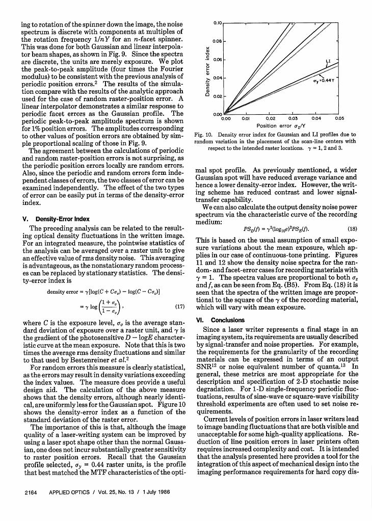
ing to rotation of the spinner down the image, the noisespectrum is discrete with components at multiples ofthe rotation frequency 1/nY for an n-facet spinner.This was done for both Gaussian and linear interpola-tor beam shapes, as shown in Fig. 9. Since the spectraare discrete, the units are merely exposure. We plotthe peak-to-peak amplitude (four times the Fouriermodulus) to be consistent with the previous analysis ofperiodic position errors.2 The results of the simula-tion compare with the results of the analytic approachused for the case of random raster-position error. Alinear interpolator demonstrates a similar response toperiodic facet errors as the Gaussian profile. Theperiodic peak-to-peak amplitude spectrum is shownfor 1% position errors. The amplitudes correspondingto other values of position errors are obtained by sim-ple proportional scaling of those in Fig. 9.

The agreement between the calculations of periodicand random raster-position errors is not surprising, asthe periodic position errors locally are random errors.Also, since the periodic and random errors form inde-pendent classes of errors, the two classes of error can beexamined independently. The effect of the two typesof error can be easily put in terms of the density-errorindex.

V. Density-Error Index

The preceding analysis can be related to the result-ing optical density fluctuations in the written image.For an integrated measure, the pointwise statistics ofthe analysis can be averaged over a raster unit to givean effective value of rms density noise. This averagingis advantageous, as the nonstationary random process-es can be replaced by stationary statistics. The densi-ty-error index is

density error = -y[log(C + Ca,) - log(C - Car)]

= y log ( + a) (17)- a)

where C is the exposure level, a, is the average stan-dard deviation of exposure over a raster unit, and y isthe gradient of the photosensitive D - logE character-istic curve at the mean exposure. Note that this is twotimes the average rms density fluctuations and similarto that used by Bestenreiner et al.

2

For random errors this measure is clearly statistical,as the errors may result in density variations exceedingthe index values. The measure does provide a usefuldesign aid. The calculation of the above measureshows that the density errors, although nearly identi-cal, are uniformly less for the Gaussian spot. Figure 10shows the density-error index as a function of thestandard deviation of the raster error.

The importance of this is that, although the imagequality of a laser-writing system can be improved byusing a laser spot shape other than the normal Gauss-ian, one does not incur substantially greater sensitivityto raster position errors. Recall that the Gaussianprofile selected, = 0.44 raster units, is the profilethat best matched the MTF characteristics of the opti-

xC

0.06 L

0.0

>0.04

o~

0.02

0.00 0.01 0.02 0.03 0.04 0.05Position error oz/Y

Fig. 10. Density error index for Gaussian and LI profiles due torandom variation in the placement of the scan-line centers with

respect to the intended raster locations. y = 1, 2 and 3.

mal spot profile. As previously mentioned, a widerGaussian spot will have reduced average variance andhence a lower density-error index. However, the writ-ing scheme has reduced contrast and lower signal-transfer capability.

We can also calculate the output density noise powerspectrum via the characteristic curve of the recordingmedium:

PSD(f) = y'(log 10 e)2PSE(f). (18)

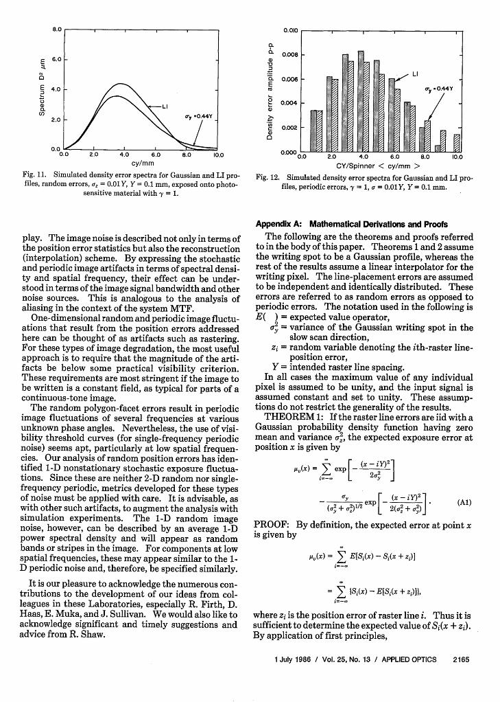
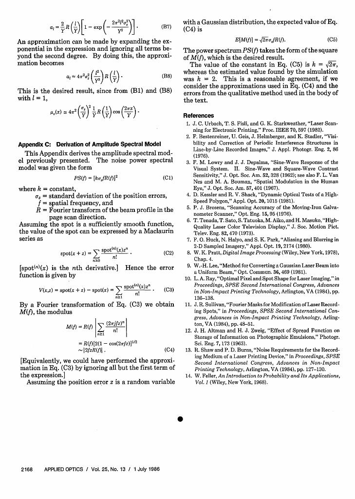
This is based on the usual assumption of small expo-sure variations about the mean exposure, which ap-plies in our case of continuous-tone printing. Figures11 and 12 show the density noise spectra for the ran-dom- and facet-error cases for recording materials withy = 1. The spectra values are proportional to both a,andf, as can be seen from Eq. (B5). From Eq. (18) it isseen that the spectra of the written image are propor-tional to the square of the y of the recording material,which will vary with mean exposure.

VI. Conclusions

Since a laser writer represents a final stage in animaging system, its requirements are usually describedby signal-transfer and noise properties. For example,the requirements for the granularity of the recordingmaterials can be expressed in terms of an outputSNR12 or noise equivalent number of quanta.'3 Ingeneral, these metrics are most appropriate for thedescription and specification of 2-D stochastic noisedegradation. For 1-D single-frequency periodic fluc-tuations, results of sine-wave or square-wave visibilitythreshold experiments are often used to set noise re-quirements.

Current levels of position errors in laser writers leadto image banding fluctuations that are both visible andunacceptable for some high-quality applications. Re-duction of line position errors in laser printers oftenrequires increased complexity and cost. It is intendedthat the analysis presented here provides a tool for theintegration of this aspect of mechanical design into theimaging performance requirements for hard copy dis-


8.0

E

E

0U)

CO,

6.0

4.0

2.0

0.0 L I I -0.0 2.0 4.0 6.0 8.0 10.0

cy/mm

Fig. 11. Simulated density error spectra for Gaussian and LI pro-files, random errors, a, = 0.01Y, Y = 0.1 mm, exposed onto photo-

sensitive material with y = 1.

play. The image noise is described not only in terms ofthe position error statistics but also the reconstruction(interpolation) scheme. By expressing the stochasticand periodic image artifacts in terms of spectral densi-ty and spatial frequency, their effect can be under-stood in terms of the image signal bandwidth and othernoise sources. This is analogous to the analysis ofaliasing in the context of the system MTF.

One-dimensional random and periodic image fluctu-ations that result from the position errors addressedhere can be thought of as artifacts such as rastering.For these types of image degradation, the most usefulapproach is to require that the magnitude of the arti-facts be below some practical visibility criterion.These requirements are most stringent if the image tobe written is a constant field, as typical for parts of acontinuous-tone image.

The random polygon-facet errors result in periodicimage fluctuations of several frequencies at variousunknown phase angles. Nevertheless, the use of visi-bility threshold curves (for single-frequency periodicnoise) seems apt, particularly at low spatial frequen-cies. Our analysis of random position errors has iden-tified -D nonstationary stochastic exposure fluctua-tions. Since these are neither 2-D random nor single-frequency periodic, metrics developed for these typesof noise must be applied with care. It is advisable, aswith other such artifacts, to augment the analysis withsimulation experiments. The -D random imagenoise, however, can be described by an average 1-Dpower spectral density and will appear as randombands or stripes in the image. For components at lowspatial frequencies, these may appear similar to the 1-D periodic noise and, therefore, be specified similarly.

It is our pleasure to acknowledge the numerous con-tributions to the development of our ideas from col-leagues in these Laboratories, especially R. Firth, D.Haas, E. Muka, and J. Sullivan. We would also like toacknowledge significant and timely suggestions andadvice from R. Shaw.

a)-D

E

CIS

CCD0

0.008

0.006

0.004

0.002

0.000 , - -:f Vo ":;. F>:x I-rl o-:d r:r.ss z 2:x I0.0 2.0 4.0 6.0 8.0 10.0

CY/Spinner < cy/mm >Fig. 12. Simulated density error spectra for Gaussian and LI pro-

files, periodic errors, -y = 1, a = .O1Y, Y = 0.1 mm.

Appendix A: Mathematical Derivations and Proofs

The following are the theorems and proofs referredto in the body of this paper. Theorems 1 and 2 assumethe writing spot to be a Gaussian profile, whereas therest of the results assume a linear interpolator for thewriting pixel. The line-placement errors are assumedto be independent and identically distributed. Theseerrors are referred to as random errors as opposed toperiodic errors. The notation used in the following isE( ) = expected value operator,

a2 = variance of the Gaussian writing spot in theslow scan direction,

Zi = random variable denoting the ith-raster line-position error,

Y = intended raster line spacing.In all cases the maximum value of any individual

pixel is assumed to be unity, and the input signal isassumed constant and set to unity. These assump-tions do not restrict the generality of the results.

THEOREM 1: If the raster line errors are iid with aGaussian probability density function having zeromean and variance 4, the expected exposure error atposition x is given by

=x 3 exp 2 2 ]L 2 J,

ay exp [ ( 2 +- ) -(aY2 + o2)1/2 [ 2 (a'+ a)J(Al)

PROOF: By definition, the expected error at point xis given by

,()= 3 E[Si(x) - Si(x + zi)]

= 3 lSi(x) - E[Si(x + i)],

where zi is the position error of raster line i. Thus it issufficient to determine the expected value of Si(x + zi).By application of first principles,


0.010

E[Si(x + Zi)] = f a exp - 2 i ]

/ 2

X exp dzi-2a,,r ( -i)2

expI - (A2)(2 +a 2)1f2 2(ay + a2) (

The result immediately follows.Expression (Al) is used extensively in calculation ofthe variance of the exposure error.

THEOREM 2: If the raster line errors are iid with aGaussian probability density function having zeromean and variance az2, the variance of the exposureerror at a position x is given by

a {(2a2 + a)1/ eXp [2a3+ay]

UY e + 2 [ } (A3)

PROOF: By assumption, the errors at each rasterline are independent, so the exposure error at a point xis the sum of independent random variables:

V1(x) = S 1(x) - Sj(X + Zi).

Hence, the variance of the exposure error is the sum ofthe variances of the random variables Vu(x).14 Leta?(x) be the variance of the random variable vi(x). Bydefinition,

ao2(x) = E[v?(x)] - A(x)

= El[Si(x) - St(x + z)] 2 - /L(x)

= S 2(x) - 2S(x)E[Sj(x + zi)]+ E[Si2(x + zi)] -,u(x),

where pti(x) is the mean value of the random variablevi(x) and is determined by a tedious but direct compu-tation. The expected value of Si(x + zi) is Eq. (A2).The expected value of S?(x + zi) is

ay~~ ( -(xiy)21(2,r2 + a;~/2P Taf+ _2 (2 a cT e x {'aa + a }

By combining the separate terms and performing somealgebraic manipulations, the resulting expression be-comes

aV(x) = (2a2 + x2)p/2 [ 2 a + a

2 F(X -iy)21ex - I~2 + a2 Ia 2 + 2

yZ LYZ

The desired quantity then results by summing over theindividual components.

The remaining theorems assume the spot shape rep-resents a linear interpolator. This is given by Eq. (14)in the text and is repeated here:

Si(x) = (1 y if (i - 1)Y< x < (i + 1)Y

0 otherwise.

THEOREM 3: If the raster-line positioning errorsare iid with a probability density function p(z), theexpected value of the exposure at any point for a con-stant input is constant. Moreover the mean exposureerror is zero.

PROOF: By applying the definition of expectationand the spot profile, the expected exposure can bewritten as

expected exposure = 3 E[Si(x + zi)]

= E J Si(x + zj)p(zL)dzL.

By assuming the sum is absolutely convergent and therandom variables zi are changed to iid, the order of thesummation can be rearranged.

Also, let wi = -iY - x. Therefore,

E jw..1 (1 + i z) p(zj)dzi

+ fl (1-Wi+l

- _ y ) p(zj)dzj

i=-E:J (1 + wy 'zi) ddz

+ J (1 - w~ y ) p(zj)dzi

= p(z)dz; = 1.

The expected exposure error is the difference in theexpected exposure with positioning errors and the ex-posure without positioning errors. Since the exposurewithout positioning errors is unity, the difference iszero.

COROLLARY 4: The expected value of the expo-sure at a point x when the jth raster line is omitted isgiven by

c-U-i) Y-x1- 0 Sj(x + X)p(X)dX.

J-(+ 1)Y-x

PROOF: This immediately follows from Theorem3.

THEOREM 5: If the raster-line positioning errorsare iid with a probability density function p(z), thevariance at any point is given by

Uo(X) £ {J- S(x + a)p(a - iY)dai

-[J S(x + ai)p(ai - iY)dai]}-


PROOF: For a fixed raster position x, the individ-ual position errors independently contribute to thetotal exposure error. As in the proof of Theorem 2, it issufficient to add the variances of the random variablesto determine the variance of the exposure error. How-ever, algebraically it is simpler to compute the variancedirectly without immediately applying the indepen-dence of the individual error terms:

Let v(x) = [si(x) - Si(X + zi)],

then

acr(x) = E[v2(x)] - p2(x)

= E[v'(x)],

where (x) = mean exposure error = 0 (Theorem 3).By expanding the expression and applying Theorem

3 to three of the resulting summations, and then by useof Corollary 4, we obtain

E[v'(x)] = -1 + E [ Si(x + zi)Sj(x + z)

= E [Z, S(x + zi)2]

-E S(x + Zi) Si(x + Xi)p(Xi)dXi

Y-+

= Z X S2 (x + a)p(ci T iY)dai

-I Y2 S(x + ai)

X Y-x Si(x + Xi)p(Xi)dX1 p(ai - iY)daci.

By a change of variable, using the definition of the spotprofile and the property that the random variables areiid, the result follows.

Appendix B: Mean Exposure Error

This Appendix provides an analytic derivation tothe spectral model of the exposure noise generated byrandom positioning errors. The model is actually aspecial case of the results of the analytic model, al-though the model captures the most useful part of theanalysis. The analysis assumes the spot shape to be aGaussian profile. The case for the linear interpolatorcan be handled similarly.

From Theorem 1 of Appendix A the mean of theerror is given by the expression

uv(x) = ao + a, cos (27)1=1

whereY

ao= _etyv(x)dx,

2

y

al =2 f2 s(x) cos (2l xdx.2

(Bi)

(B2)

(B3)

It can be easily verified that ao = 0. To find al we notethat

2y Yr @ [(x-iY)2 1 2x1x

2=Y + exp -2(a Z +2a)J o Y )

EX [ -2y2 )exp(X iy)2 yxx2 I=YJ

= all + a21.

Since Ys(x) is an absolutely convergent series (withprobability 1), the terms may be rearranged in anymanner. In particular, the series may be broken intotwo pieces, and the coefficients of the Fourier seriescan be computed by individually integrating with re-spect to each of the pieces and then adding the results.Let the second part of the expression be given by theseries

a 2 Jexp | -cr 2 cos 2y X dx

_2 ( 1 x2 2,rl\= ye exp C2)cos y x) dx,

where we have interchanged the order of the summa-tion and the integration. The resulting summation offinite integrals can be converted to a single integralwith the region of intergation over the entire line.Indeed, the expression is simply

2j>cr,, ( -2a2 12,ir 2

a2 = y exp YY y2(B4)

where the latter result is derived using integral tables.Similarly, all is found to be

2jAcr,, F ~2ir212(4r2 + 2) 1a11 Y exp y2 ,

Finally,

a, = all + a21

- 2CrY exp t27r 2a 1) 2 1 - exp t2 7 r 22)]2'

(B5)

(B6)

A,(x) = E x- cr- exp [ <-c JfSince p,(x) is a periodic function with period equal tothe spacing between adjacent raster lines (i.e., Y), itcan be expanded as a Fourier series of the form

We define R(f) as the Fourier transform of the spotS(x), and since a Gaussian spot of radius ay has aGaussian Fourier transform,

R(f) = Hcray exp (-27r2 yf 2)

Equation (B6) may be recast as


a,= R () [1 - exp 2 (B7)

An approximation can be made by expanding the ex-ponential in the expression and ignoring all terms be-yond the second degree. By doing this, the approxi-mation becomes

al - 4ir2cr2 (-t 3) R (y)* (B8)

This is the desired result, since from (B) and (B8)with 1 = 1,

gJ(x) 4.72 (cr)2 ;R (y) cos ( -

Appendix C: Derivation of Amplitude Spectral Model

This Appendix derives the amplitude spectral mod-el previously presented. The noise power spectralmodel was given the form

PS(f) = [kcrzfR(f)]2 (Cl)

where k = constant,az = standard deviation of the position errors,f = spatial frequency, and

R = Fourier transform of the beam profile in thepage scan direction.

Assuming the spot is a sufficiently smooth function,the value of the spot can be expressed by a Maclaurinseries as

spot(X + z) =3 sPot~')(x)zn (C2)n20

[spot(n)(x) is the nth derivative.] Hence the errorfunction is given by

V(x,z) = spot(x + Z) - spot(X) = n (Cnn1

By a Fourier transformation of Eq. (C3) we obtainM(f), the modulus

M(f) = R(f) 3, (2 rjfz) nn>1

= R(f)[2(1- cos(2rfz)]1/2

-1 2fzR(f)l .(C4)

[Equivalently, we could have performed the approxi-mation in Eq. (C3) by ignoring all but the first term ofthe expression.]

Assuming the position error z is a random variable

with a Gaussian distribution, the expected value of Eq.(C4) is

E[M(f)] = cr2 fR(f). (C5)

The power spectrum PS(f) takes the form of the squareof M(f), which is the desired result.

The value of the constant in Eq. (C5) is k = 2,whereas the estimated value found by the simulationwas k = 2. This is a reasonable agreement, if weconsider the approximations used in Eq. (C4) and theerrors from the qualitative method used in the body ofthe text.

References1. J. C. Urbach, T. S. Fish, and G. K. Starkweather, "Laser Scan-

ning for Electronic Printing," Proc. IEEE 70, 597 (1982).2. F. Bestenreiner, U. Geis, J. Helmberger, and K. Stadler, "Visi-

bility and Correction of Periodic Interference Structures inLine-by-Line Recorded Images," J. Appl. Photogr. Eng. 2, 86(1976).

3. F. M. Lowry and J. J. Depalma, "Sine-Wave Response of theVisual System. II. Sine-Wave and Square-Wave ContrastSensitivity," J. Opt. Soc. Am. 52, 328 (1962); see also F. L. VanNes and M. A. Bouman, "Spatial Modulation in the HumanEye," J. Opt. Soc. Am. 57,401 (1967).

4. D. Kessler and R. V. Shack, "Dynamic Optical Tests of a High-Speed Polygon," Appl. Opt. 20, 1015 (1981).

5. P. J. Brosens, "Scanning Accuracy of the Moving-Iron Galva-nometer Scanner," Opt. Eng. 15, 95 (1976).

6. T. Tenada, T. Sato, S. Tatuoka, M. Aiko, and H. Masuko, "High-Quality Laser Color Television Display," J. Soc. Motion Pict.Telev. Eng. 82, 470 (1973).

7. F. 0. Huck, N. Halyo, and S. K. Park, "Aliasing and Blurring in2-D Sampled Imagery," Appl. Opt. 19, 2174 (1980).

8. W. K. Pratt, Digital Image Processing (Wiley, New York, 1978),Chap. 4.

9. W.-H. Lee, "Method for Converting a Gaussian Laser Beam intoa Uniform Beam," Opt. Commun. 36, 469 (1981).

10. L. A. Ray, "Optimal Pixel and Spot Shape for Laser Imaging," inProceedings, SPSE Second International Congress, Advancesin Non-Impact Printing Technology, Arlington, VA (1984), pp.136-138.

11. J. R. Sullivan, "Fourier Masks for Modification of Laser Record-ing Spots," in Proceedings, SPSE Second International Con-gress, Advances in Non-Impact Printing Technology, Arling-ton, VA (1984), pp. 48-51.

12. J. H. Altman and H. J. Zweig, "Effect of Spread Function onStorage of Information on Photographic Emulsions," Photogr.Sci. Eng. 7, 173 (1963).

13. R. Shaw and P. D. Burns, "Noise Requirements for the Record-ing Medium of a Laser Printing Device," in Proceedings, SPSESecond International Congress, Advances in Non-ImpactPrinting Technology, Arlington, VA (1984), pp. 127-130.

14. W. Feller, An Introduction to Probability and Its Applications,Vol. 1 (Wiley, New York, 1968).


analysis of image noise due to position errors in laser writers

Documents