analysis of heterogeneous patterns and social dynamics in human

Analysis of Heterogeneous Patterns andSocial Dynamics in Human

Communication

A Senior Project submitted toThe Division of Science, Mathematics, and Computing

ofBard College

byZhechao Zhou

Annandale-on-Hudson, New YorkApril, 2009

Abstract

Vertex connectivities in complex networks are widely recognized to display a scale-free power-law distribution generated by network growth and node preferential attach-ment. Observation of the power-law distribution of tie weights together with the over-representation of network motifs in social networks suggests the existence of non-trivialnetwork mechanisms beyond node level. This project investigates the existing social net-work theories and proposes a stochastic model for weighted scale-free networks in whichhigh-weight ties are more likely to grow using random walk as an approach. The modelreproduces the observed scale-free weight distributions from a pure dyad perspective andconcavity of the distribution curve as the consequence of triad embeddedness. Computersimulations of both processes confirm the theoretical predictions with the statistical anal-ysis of a communication network among millions of individuals. This project, as part of anongoing NSF-funded social network study, contributes to the dynamic analysis of processesof tie formation, stability and change at the dyad and triad level and leads to a system-atic understanding of the fundamental processes and interdependencies underlying socialnetwork dynamics that has deep implications in large-scale human interaction behavior.

Contents

Abstract 1

Dedication 5

Acknowledgments 6

1 Introduction 7

2 Preliminaries 102.1 Definition . . . . . . . . . . . . . . . . . . . . . . . . . . . . . . . . . . . . . 102.2 Theories, models and mechanisms . . . . . . . . . . . . . . . . . . . . . . . . 11

2.2.1 A Brief Introduction of Social Balance Theory . . . . . . . . . . . . 112.2.2 Other Relevant Factors . . . . . . . . . . . . . . . . . . . . . . . . . 122.2.3 Master Equation . . . . . . . . . . . . . . . . . . . . . . . . . . . . . 13

2.3 Data . . . . . . . . . . . . . . . . . . . . . . . . . . . . . . . . . . . . . . . . 14

3 Continuous-Time Random Walks and Waiting Time 17

4 Dyadic Dynamics 21

5 Triadic Dynamics 28

6 Conclusion and Future Work 33

7 Appendix 357.1 Code . . . . . . . . . . . . . . . . . . . . . . . . . . . . . . . . . . . . . . . . 35

7.1.1 Dyad process simulation . . . . . . . . . . . . . . . . . . . . . . . . . 357.1.2 Triad process simulation . . . . . . . . . . . . . . . . . . . . . . . . . 37

Contents 3

7.1.3 Triad weight distribution code . . . . . . . . . . . . . . . . . . . . . 407.2 Other results in triads . . . . . . . . . . . . . . . . . . . . . . . . . . . . . . 43

Bibliography 46

List of Figures

2.1.1 16 types of triads. . . . . . . . . . . . . . . . . . . . . . . . . . . . . . . . . 112.3.1 In and out degree distribution of the nodes in the data. . . . . . . . . . . . 15

3.0.1 Waiting time distribution generated from 6 week cell phone records. . . . . 19

4.0.1 Distribution of dyad weights from the data. . . . . . . . . . . . . . . . . . . 254.0.2 The comparison of a computer-simulated weight distribution and the real-

world data. The simulation is generated for 5000 nodes, ε = 0.01, overT = 200 time steps and m = 2× 106 every step. . . . . . . . . . . . . . . . . 26

4.0.3 Other potential evolving probability function trial results: w2

t2(yellow), w

0.4

t

(light blue), w0.7

t (pink), w0.9

t (blue), wt (red) compared with the real data

in green. . . . . . . . . . . . . . . . . . . . . . . . . . . . . . . . . . . . . . . 27

5.0.1 P(a,b,c)-abc plot. P(a,b,c) spans over the 1.1–1.5 slope range. . . . . . . . . 295.0.2 The comparison of a computer-simulated weight distribution based on the

dyad, triad mechanisms and the real-world data. The triadic simulation isgenerated for 500 nodes, ε = 0.01, δ = 0.0012, over T = 350 time steps andm = 75000 every step. . . . . . . . . . . . . . . . . . . . . . . . . . . . . . . 32

7.2.1 Triad weight distribution from the data. The three axes represents theweights of the three combining dyads. The color scale indicates log(frequency). 44

7.2.2 Triad weight distribution from the simulation. The three axes represents theweights of the three combining dyads. The color scale indicates log(frequency). 45

Dedication

To my parents, for their generous love and support

Acknowledgments

I would like to express my sincerest gratitude to all the those who helped me in completingthis thesis. I want to thank my advisors Matthew Deady and Gregory Landweber for theirefforts in learning and understanding the material of this project despite most of it beingnew to them. I am grateful to Matthew for his academic advising not only over the courseof the senior year, but also every step along my Bard experience. Greg must also be dulythanked here for his assistance with computer programming. The mathematical clarity ofthis project benefits from his comments. I also thank Christian Bracher for being on myboard and giving feedbacks.

I would like to extend my gratitude to Zoltan Toroczkai of University of Notre Dame,who makes this cool project possible, for teaching me how to do research and being in-credibly nice. He is and will remain the knowledgable network guru in my mind.

Burton Brody is not to be forgotten here for sharing his experience, knowledge andgood sense of humor. I wish I could have more classes with him.

There are many others, but they know who they are.

1Introduction

Complex networks describe a wide range of systems of high technological and intellectual

importance. For example, the Internet is a complex network of routers and computers

connected by physical or wireless links; the cell is best described as a complex network

of chemicals connected by chemical reactions; opinions and ideas are spread through the

social network, whose nodes are human beings and whose edges consist of various social

relationships. These systems represent just a few of many complex networks that prompted

the scientific investigation into the mechanism that determines the topology of complex

networks in recent years.

Traditionally, the study of complex networks has been the territory of graph theory. In

the 1950s the modeling of large-scale networks as random graphs with no apparent design

principles was first studied by Erdos and Renyi (see [6]). According to the Erdos-Renyi

model, the network starts with N nodes and connects every pair of nodes with probability

p, creating a graph with approximately pN(N − 1)/2 edges distributed randomly. In a

random graph, since the edges are placed randomly, the majority of nodes have approx-

imately the same degree k (the number of connecting neighbors), close to the average

1. INTRODUCTION 8

degree 〈k〉 of the network. The degree distribution of a random graph follows a Poisson

distribution with a peak at 〈k〉.

In the past few years, motivated by the emergence of large databases collected by com-

puters and the increasing computing power available, many new statistical measures on

complex networks have been proposed and conducted in depth. For a large number of

networks, such as the World Wide Web, and protein interaction networks, there exists

strong evidence that the degree distribution has a power-law tail P (k) ∼ k−γ , where

γ is between 2 and 3 for most cases. Such networks are called scale-free networks. The

Barabasi-Albert model (see [3]) presents the most simple self-organizing mechanism of the

scale-free structure. At each time step a new node is added and connected to old nodes

of the network through m new links. The probability of an old node being linked with

the new node is proportional to the total number of the connections with this node. It

establishes P (k) ∼ k−γ at long times and large connectivities.

This discovery of the power-law degree distribution indicates that the topology and

evolution of complex networks are governed by robust non-random organizing principles.

And the tools of statistical mechanics offer an ideal framework for studying complex

networks. The fact that some motifs such as triads and clusters are over-represented in real-

world networks as compared to randomized networks with the same degree distribution

suggests some fundamental and potentially generic features of network dynamics. Yet,

the mechanism responsible for these marked non-random features remains unknown. This

project will be a first attempt to unveil the weighted dyad and triad formulation mechanism

in complex networks with the focus on the discussion of social networks.

In Chapter 2 we first introduce the definitions of the technical terms in this project.

A detailed review of various theoretical and empirical results from the existing journal

literature follows to establish and justify the assumptions made for the model later on in

1. INTRODUCTION 9

this project. In the second section, we introduce the master equation as the major method

employed in this project and discuss the data used to test the theoretical model.

In Chapter 3 we discuss continuous random walks and waiting time density. We will

show the whole calculation to derive the general expression for the probability of walking

n steps in time t and the specific one given the waiting time density function A× t−α from

the empirical data.

In Chapter 4 we set up the basic assumptions of the purely dyadic model, explain the

reasoning behind the calculation and derive the conclusion. We also employ Monte Carlo

simulation to test the result and compare it with the analysis of the real-world data.

In Chapter 5 we discuss the modified model of dyad evolution within the context of local

communities. We will explain the extra assumption being made and its relationship with

social balance theory. The result of the triadic process is presented numerically through

computer simulation.

2Preliminaries

2.1 Definition

In network science, a node is an agent in the network. A useful way to think about

the network is as a structure revealed through undirectional or directional dyadic ties

(edges) among two nodes. The degree of a node is the number of edges that are incident

with it, or the number of nodes adjacent to it. A dyad in sociology is used to describe

the relationship of two nodes. The dyads may carry weights to show relationship types,

frequency, tie strengths or some other dyadic properties.

Triads consist of three nodes and the possible dyadic relationships between any two

of them. A dyad is usually embedded in more than one triad. Social scientists classify

triads into 16 different types regardless of node combinations [16]. In this project, we

use a generalized definition of the triads as the combination of the three weighted dyads

between any three nodes in the network.

The clustering coefficient of a node in a graph quantifies how close the node and its

neighbors are to being a clique (complete graph). The clustering coefficient is a direct

concept of how a single node is organized into a triad. Suppose a selected node i in the

2. PRELIMINARIES 11

Figure 2.1.1. 16 types of triads.

network has ki edges which connect it to ki other nodes. The clustering coefficient is the

ratio between the number Ei of edges that actually exist between these ki nodes and the

total possible ki(ki − 1)/2 edges, Ci = 2Eiki(ki−1) . The clustering coefficient for the whole

system is given as the average of the clustering coefficient for each node.

2.2 Theories, models and mechanisms

2.2.1 A Brief Introduction of Social Balance Theory

In real world social networks, social cliques are often observed. People who share interests,

views, purposes, patterns of behavior, or ethnicity tend to formulate strong ties with the

other members in the groups which in turn shape their actions. Therefore some motifs

such as triads and clusters are over-represented in real-world networks as compared to

randomized networks with the same degree distribution [13]. And some triadic congura-

tions such as the non-transitive uni-direction triad 030C are very rare in the networks

[17]. Although the Barabasi-Albert model has successfully explained the scale-free nature

of many networks on node level, the empirical evidence of a big number of triads well above

2. PRELIMINARIES 12

random expectations in the vast majority of real networks has brought the multi-agent

network dynamics beyond node level into attention.

Triads in complex networks are recognized as the building blocks in the composition of

recurring subgraphs, closely related to the large-scale organization of complex networks.

Heider [8] first developed the basic components of structural balance theory as a framework

for studying the structural arrangement in social networks. An edge ij is positive if nodes

i and j are friends, and negative if i and j are enemies. The triad ijk is balanced if the sign

of the product of the links in the triad is positive. A balanced triad fulfills the following

adage: a friend of my friend is my friend; an enemy of my friend is my enemy; a friend

of my enemy is my enemy; an enemy of my enemy is my friend. A network is balanced if

each constituent triad is balanced. Cartwright and Harary [5] generalized the definition of

a balanced network to that every cycle in the network is balanced. The cycle-based and

triad-based definitions of balance are demonstrated to be equivalent on complete graphs.

Antal [1],[2] presented a simple rate-equation model for social dynamics in which both

friendly and unfriendly links evolve following the assumption that people naturally tend

to avoid imbalanced relationships. The study shows that a balanced network tends to be

more stable while unbalanced networks tend to be unstable. A finite network always falls

into a socially-balanced absorbing state where no imbalanced triads remain after certain

amount of time. Balance theory predicts that triads tend to form a fully reciprocal closure

or dissolve. The resulting social networks display a strong local community structure and

relatively weak inter-community connections.

2.2.2 Other Relevant Factors

Tie formulation (meaning two nodes establish a new connection) and tie persistence (mean-

ing the established connections continue to exist or strengthen by increasing weights) are

not only subject to social balance forces but also to other factors. Hidalgo and Rodriguez-

2. PRELIMINARIES 13

Sickert study the coupling between the structure of the network and the temporal stability

of its links [9]. It shows that persistent links tend to be reciprocal and more common for

people with low degrees and high clustering coefficients from ten panels of mobile phone

data of a year. Reciprocity tends to be the strongest predictor of tie persistence in social

networks among other dyadic characters.

The probability that two nodes are connected by a link follows a gravity model, i.e.

decreasing as geographical distance squared [11]. Communication triangles are not only

composed of geographically adjacent nodes but they may extend over long distances.

Shorter links have higher probabilities of belonging to triangles than longer links. Local

groups are characterized by short communication and high clustering coefficients, and

long-distance groups features longer communication and low clustering coefficients. In

a communication network the majority of the strong ties are found within the clusters,

indicating that users spend most of their on-air time talking to members of their immediate

circle of friends. In contrast, most links connecting different communities are significantly

weaker than the links within the communities [14].

2.2.3 Master Equation

The notion of a random process grows from an attempt to describe microscopically complex

processes by statistical equations of evolution. A mathematical model for the random

evolution of a memory-less system, that is, one for which the likelihood of a given future

state, at any given moment, depends only on its present state, and not on any past states,

is called a Markov process. In statistical physics a master equation is widely used to

describe a Markov process. The master equation gives the rate of change of the continuous

probability function P (n, t) due to transitions into the state n from all other states and

due to transitions out of state n into all other states, [15]

∂P (n, t)∂t

=∑m=1

[P (m, t)wm,n(t)− P (n, t)wn,m(t)],

2. PRELIMINARIES 14

where wm,n(t) is the probability of a transition from state m to state n during the time

interval ∆t.

2.3 Data

Although individual human behavior is rather complex and unpredictable, there are quan-

titative measures characteristic to large collectives of humans that are reproducible and

thus subject to measurement. In some sense, a large population is similar to an ideal gas

system in which the measurement and modeling on a single molecule’s movement is much

harder than on the macro-scale of the whole system. In the past, social scientific research

on human behavior and social networks has been rather limited due to lack of high-quality

large-scale data and quantitive methods to analyze such data. In general, data obtained

through surveys is usually small, non-longitudinal (independent of time) and biased by

the existence of the observer and the methods in the experiment.

The data in this project are generated from a nationwide cell-phone network of about 6.7

million users in an industrialized country. The operation of cell-phone systems generates

enormous amounts of information on human activity patterns. The customer bases of cell

phone companies range from hundreds of thousands to millions, therefore such large-scale

data sets can provide exceptional statistics on social networks and human dynamics. The

second advantage of this type of data is that it is purely observational; therefore, it is

completely void of any observational bias.

The social network is a structure revealed through dyadic communication among peo-

ple. If A and B have communicated with each other (through voice calls, SMSs) within

a given time frame Tw, then we assume that a tie exists between them. The frequency of

communication interactions between them defines tie strength. Repeating this construc-

tion process with all pairs, one obtains the full social network of the population during a

particular time window. In sum, the full social network in a given time period can be de-

2. PRELIMINARIES 15

1

10

100

1000

10000

100000

1e+06

1e+07

1 10 100 1000 10000

"in_degree.txt""out_degree.txt"

Figure 2.3.1. In and out degree distribution of the nodes in the data.

scribed by the nodes (users), and the tie strengths (captured by frequency measures). The

analysis of this network obtained from a given time frame will provide us with extensive

cross-sectional information, while the study of the time evolution of this network will give

us unprecedented longitudinal information.

The data include information of the caller, callee, type (voice calls or SMSs), number

of calls between the caller and callee, and total duration in seconds. In total, 24,441,476

entries are collected of all the communication events in the network. The distribution for

the degree has a fat tail slowly decreasing to zero with some out-degree noise near the end

of the tail (see Figure 2.3.1). So the network is a scale-free network.

The mobile network captures only a subset of all interactions between individuals, a

detailed mapping of which would include face-to-face, e-mail, and land line communica-

tions as well. Yet although mobile phone data capture just a slice of total communications,

research on media multiplexity suggests that the use of one medium for communication

2. PRELIMINARIES 16

between two people implies communications by other means as well [7]. Moreover, because

of the absence of cell-phone directory listings, these data effectively map the network of

trusted interactions from the overall social network. Therefore the data can be used as a

proxy of the communication network between individuals.

3Continuous-Time Random Walks and WaitingTime

A random walk is a mathematical formalization of a trajectory that consists of taking

successive random steps. An elementary example of a random walk is the binomial random

walk along the integer line, which starts at S0 = 0 and at each step moves by ±1 with

equal probability. The steps are statistically independent. Sn is the position of the walker

on the line after n step. It is not hard to see that the expectation value E(Sn) = 0 and

E(S2n) = n.

We consider a random walk for which the times Tj between successive steps are in-

dependent, identically distributed random variables, with a common probability density

function ψ(t), called the waiting-time density. Suppose that we allow a continuous-time

random walk to begin at time t = 0. Let ψn(t) denote the probability density function for

the time at which the nth step occurs, so that ψ1(t) = ψ(t). From the independence of

the times between steps, we have the recurrence relation

ψn(t) =∫ t

0ψ(τ)ψn−1(t− τ)dτ. (3.1)

The convolution integral in Equation 3.1 may be factorized by applying the Laplace trans-

formation. The Laplace transformation of the function φ is

3. CONTINUOUS-TIME RANDOM WALKS AND WAITING TIME 18

φ(s) = L [φ(t)] =∫ ∞

0e−stφ(t)dt. (3.2)

Applying the Laplace transformation to Equation 3.1,

ψn(s) = L [ψn(t)]

= L [ψ(t)]L [ψn−1(t)]

= L [ψ(t)]2L [ψn−2(t)]

...

= L [ψ(t)]n

= [ψ(s)]n. (3.3)

Let N(t) denote the number of steps taken up to time t. To have N(t) = n, the walker

has to make n steps in some time interval (0, t′) and then make no further steps in the

time interval (t′, t). Since ψn is the probability density function for the time of occurrence

of the nth step and

Ψ(t) = 1−∫ t

0ψ(t′)dt′ =

∫ ∞t

ψ(t′)dt′ (3.4)

is the probability that a walker arriving at a site pauses for at least time t, it follows that

Pr{N(t) = n} =∫ t

0ψn(t′)Ψ(t− t′)dt′. (3.5)

By Equation 3.3 we know ψn(s) = [ψ(s)]n, and noting that

Ψ(s) = L [Ψ(t)] = s−1[1− ψ(s)], (3.6)

we find that

L [Pr{N(t) = n}] =ψ(s)n[1− ψ(s)]

s. (3.7)

Current models of human activity are based on Poisson processes, and assume that

in a dt time interval an individual engages in a specific actions with probability q dt,


10000

100000

1e+06

1e+07

1 10 100

frequ

ency

waiting time in minutes

dataslope -0.95

Figure 3.0.1. Waiting time distribution generated from 6 week cell phone records.

where q is the overall average frequency of the monitored activity. In contrast, there is

increasing evidence that the timing of many human activities, ranging from communication

to entertainment and work patterns, follow non-Poisson statistics, characterized by bursts

of rapidly occuring events separated by long periods of inactivity. The bursty nature of

human behaviour is a consequence of a decision-based queueing process. When individuals

execute tasks based on some perceived priority, the timing of the tasks will be heavy tailed

(see [4]). This model predicts that the time interval between two consecutive actions by

the same individual, called the waiting time, follows an exponential distribution. The

measurement of our data confirms this conclusion (Figure 3.0.1).

In our case, the waiting time probability density function is ψ(t) = A× t−α, with A as

a constant. The Laplace transformation of the function is

L [ψ(t)] = ψ(s) = Asα−1Γ(1− α), (3.8)


where Γ(x) is the Gamma function. By Equation 3.7, applying the inverse Laplace trans-

formation, we get

Pr{N(t) = w} = L −1[ ψ(s)n[1− ψ(s)]

s

]= [At1−αΓ(1− α)]w+1

[1

Γ(2 + w − α− wα)− At1−αΓ(1− α)

Γ(3 + w − 2α− wα)

].

(3.9)

This is the probability of having exactly w events within time t given the waiting time

probability density ψ(t) = A×t−α. In the next chapter, we will use this result to construct

our first model on dyadic growth.

4Dyadic Dynamics

Suppose the network has n nodes at time t. Let p(w, ti, t) be the probability that an edge i

introduced at time ti has weight w at time t. If the system has a fixed number of nodes, all

the nodes are introduced at time 0 with no edges (trivial graph). In every step, m edges

out of n(n − 1)/2 edges are randomly selected. We view the weight increasing process

of a selected dyad as a random walk for which the waiting time probability density is

ψ(t) = A× t−α.

By Equation 3.9,

Pr{N(t−1) = w} = [A(t−1)1−αΓ(1−α)]w+1

[1

Γ(2 + w − α− wα)− A(t− 1)1−αΓ(1− α)

Γ(3 + w − 2α− wα)

],

(4.1)

and

Pr{N(t) = w+ 1} = [At1−αΓ(1− α)]w+2

[1

Γ(3 + w − 2α− wα)− At1−αΓ(1− α)

Γ(4 + w − 3α− wα)

].

(4.2)

4. DYADIC DYNAMICS 22

Thus the possibility for a single event to happen within one time step is approximately

the quotient of the two above,

p ≈ Pr{N(t) = w + 1}Pr{N(t− 1) = w}

= A(t− 1)wα−wtw−wα−α+1Γ(1− α)1

Γ(2+w−α−wα) −At1−αΓ(1−α)

Γ(3+w−2α−wα)

1Γ(1+w−wα) −

A(t−1)1−αΓ(1−α)Γ(2+w−α−wα)

. (4.3)

This is the analytical solution of the possibility for a single event to happen within one

time step. However, we will use a much simpler alternative function p = w/t in the model

to get an analytical weight distribution approximate to the real distribution. We now show

that this function is actually a reasonable assumption for the model.

Suppose w events have happened before time step t. The probability of the next event

happening at time step t+ n, based on the alternative function, is

P (w + 1; t+ n) = P (w; t)(

1− w

t+ 1

)(1− w

t+ 2

). . .

(1− w

t+ n− 1

)w + 1t+ n

, (4.4)

and we have

P (w + 1; t+ n+ 1) = P (w; t)(

1− w

t+ 1

)(1− w

t+ 2

). . .

(1− w

t+ n

)w + 1

t+ n+ 1. (4.5)

By Equation 4.4 and Equation 4.5,

P (w + 1; t+ n)P (w + 1; t+ n+ 1)

=t+ n+ 1t+ n− w

. (4.6)

By iterating Equation 4.6,

P (w + 1; t+ n)P (w + 1; t+ n′)

=t+ n+ 1t+ n− w

t+ n+ 2t+ n+ 1− w

· · · t+ n′

t+ n′ − 1− w. (4.7)

Since we can arbitrarily set the time when the w-th events happens to be zero, Equation

4.7 becomesP (w + 1;n)P (w + 1;n′)

=(n+ 1)(n+ 2) · · ·n′

(n− w)(n+ 1− w) · · · (n′ − 1− w). (4.8)

When w = 0,P (w + 1;n)P (w + 1;n′)

=(n+ 1)(n+ 2) · · ·n′

n(n+ 1) · · · (n′ − 1)=( nn′

)−1. (4.9)


When w = 1,

P (w + 1;n)P (w + 1;n′)

=(n+ 1)(n+ 2) · · ·n′

(n− 1)n · · · (n′ − 2)∼( nn′

)−2. (4.10)

In general,

P (w + 1;n)P (w + 1;n′)

∼( nn′

)−(w+1), (4.11)

where P (w;n) can be interpreted as the waiting time distribution between w-th event and

(w + 1)-th event. The exponential form of Equation 4.11 is consistent with the observed

scale-free waiting time distribution. Therefore wt can serve as a simplification of Equation

4.3.

Back to the model, at time t, if the weight wi of a selected edge i is not zero, wi increases

by 1 with a probability wit following the previous argument; otherwise it stays the same.

If wi = 0, the probability of evolving is εt where ε is some real number between 0 and 1.

Consequently the master equation governing p(w, ti, t) has the form

p(w, ti, t+ 1) ={

w−1t p(w − 1, ti, t) +

(1− w

t

)p(w, ti, t) if w > 1,

εtp(0, ti, t) +

(1− 1

t

)p(1, ti, t) if w = 1.

(4.12)

It is not always easy to measure the newly formed nodes in a large network. In the general

case, the proportion of weight w edges in the whole system P (w, t) at time t is directly

measurable and thus we are more interested in solving P (w, t). Since 0 < P (w, t) < 1, for

mathematical convenience, let

P (w, t) =1t

∑ti

p(w, ti, t). (4.13)

Summing Equation 4.12 up from ti = 1 to ti = t, when w > 1, we get

(t+ 1)P (w, t+ 1)− p(w, t+ 1, t+ 1) =w − 1t

tP (w − 1, t) +(

1− w

t

)tP (w, t).

Reducing the right side of the equation,

(t+ 1)P (w, t+ 1)− p(w, t+ 1, t+ 1) = (w − 1)P (w − 1, t) + (t− w)P (w, t). (4.14)


Newly added nodes have no edges to any other nodes in the network. When w is not zero,

p(w, t+ 1, t+ 1) = 0. Assuming the limit P (w) = P (w, t −→∞) exists and t[P (w, t+ 1)−

P (w, t)] −→ 0 as t −→∞, we get

(w + 1)P (w) = (w − 1)P (w − 1). (4.15)

When w = 1, following the similar steps above,

(t+ 1)P (1, t+ 1)− p(1, t+ 1, t+ 1) = εP (0, t) + (t− 1)P (1, t).

For t −→∞,

2P (1) = εP (0). (4.16)

If P (1) is some constant C1,

P (w) =2C1

w(w + 1)=

εP (0)w(w + 1)

∼ w−2. (4.17)

The exponent measured from real data is about −1.95 (see Figure 4.0.1). To verify the

model, we used a Monte Carlo simulation to generate the weight distribution following

the assumptions of the model and compared it with the real-world data (see Figure 4.0.2,

for code see 7.1.1). For every time step in the simulation process, a fixed number of node

pairs are randomly picked from all the nodes. For each of these pairs, we compare the ratio

of the existing weights between the two nodes to the maximum possible weights w = t at

time step t with a generated random number between 0 and 1 to determine whether the

weight of this pair increases by 1.

So far the prediction of the dyad model is roughly consistent with the measurement

from the real data. However, the dyad model has its deficiencies that lead us to the next

chapter on triadic dynamics.


1

10

100

1000

10000

100000

1e+06

1e+07

1 10 100 1000

P(w)

w

dataslope -1.95

Figure 4.0.1. Distribution of dyad weights from the data.


100

1000

10000

100000

1e+06

1e+07

1 10 100

P(w

)

w

datasimulation

slope -2

Figure 4.0.2. The comparison of a computer-simulated weight distribution and the real-world data. The simulation is generated for 5000 nodes, ε = 0.01, over T = 200 time stepsand m = 2× 106 every step.


1

10

100

1000

10000

100000

1e+06

1e+07

1 10 100

P(w)

w

Figure 4.0.3. Other potential evolving probability function trial results: w2

t2(yellow), w0.4

t

(light blue), w0.7

t (pink), w0.9

t (blue), wt (red) compared with the real data in green.

5Triadic Dynamics

In real world networks, motifs such as triads and clusters are over-represented as compared

to randomized networks with the same degree distribution, which we also observe from

our data. If the triads in the network are purely random combinations of the weighted

dyads, then the possibility of a triad containing three weighted dyads a,b,c is

P (a, b, c) = P (a)P (b)P (c) = (abc)−γ .

P (a, b, c) should follow a scale-free distribution with the same slope −γ. However P (a, b, c)

in Figure 5.0.1 from the real data is inconsistent with this expectation. This indicates that

the weighted dyads are organized into the community structure following some non-trivial

mechanisms.

Sociological theories that address the dynamics of social ties postulate that individual

commonalities cause tie formation or rational people build up ties for strategic reasons

to maximize utility, such as networking with popular (high-degree) people. Other theories

suggest that processes of dyad formation and persistence are not only a function of purely

node characters and dyadic factors but are also affected by the embeddedness of dyads in

triadic congurations from a balance view (see 2.2.1 for social balance theory). For example,

5. TRIADIC DYNAMICS 29

1

10

100

1000

10000

100000

1e+06

1e+07

1 10 100 1000 10000 100000 1e+06

P(ab

c)

abc

dataslope -1.5slope -1.1

Figure 5.0.1. P(a,b,c)-abc plot. P(a,b,c) spans over the 1.1–1.5 slope range.

job hunters network with the employees in the industry for advice on their credentials.

They may also build up the relationships in order to be introduced to the third parties

who make decisions in hiring. Moreover, the strength of a tie between two nodes increases

with the overlap of their friendship circles in general [14]. The overlap of friendship circles

may imply that the two nodes belong to the same community. The real explanation of the

dyad formation process may be a combination of the purely dyadic view on dyad factors

(such as reciprocity and strength) and the global view on dyadic embeddedness in triads

and even higher-order network structures.

Therefore following the rationale above, we modify the model in the previous chapter

by adding one more assumption: two nodes are more likely to form or maintain a tie

if they have at least one common friend, a third node that is connected with both. To

quantify a relationship, we label a tie as +1 if the two nodes are friends, −1 if they are

enemies following the notation used in social balance theory. A triad ABC is balanced if


the sign of the product of the three ties equals +1. If the cell phone calling records capture

mostly positive ties in the network (wAB > 0 implying sAB = +1), the new assumption

is equivalent to the general balancing rules of social triads. For a triad of three nodes A,

B, C, if sAB = +1, sAC = +1 and sBC = −1, B and C should have a high probability to

become friends (sBC = +1) in order to balance the triad according to the theory. Similarly,

the modified model states that it is likely to observe tie BC from the data given non-zero

wAB and wAC . On the other hand, the balancing theory suggests that sAB or sAC might

turn negative to balance the triad. In the modified model, wAB and wAC are less likely

to increase, which implies sAB = −1 or sAC = −1 if wBC is zero. Moreover, our model

is able to study the “positiveness” of the ties quantitatively compared to the qualitative

notation in the existing social balance models.

Let p(w, ti, t) be the probability that an edge i introduced at time ti has weight wi at

time t. In every step, m edges out of n(n− 1)/2 edges are randomly selected. At time t, if

the weight wi of a selected edge i is not 0, wi increases by 1 following a new probability

density functionwi + δ

∑c(wj + wk)t

, (5.1)

where∑

c(wj + wk) is the sum of the dyad weights between A and B, the two nodes of

edge i, and their common friends, respectively. If C is a common friend of A and B, the

tie weights wj between A and C and wk between B and C are both non-zero and included

in the sum. δ is the coefficient that measures the contribution of triads to the dyad. If

wi = 0 and∑

c(wj + wk) is also zero (A and B have no common friend), the probability

of evolving is εt where ε is some real number between 0 and 1. Consequently the master

equation governing p(wi, ti, t) has the form

p(wi, ti, t+1) =

wi−1+δ

Pc(wj+wk)t p(wi − 1, ti, t) +

(1− wi+δ

Pc(wj+wk)t

)p(wi, ti, t) if wi > 1,

δPc(wj+wk)t p(0, ti, t) + (1− 1+

Pc(wj+wk)t )p(1, ti, t) if wi = 1 and

∑c(wj + wk) 6= 0,

εtp(0, ti, t) +

(1− 1

t

)p(1, ti, t) if wi = 1 and

∑c(wj + wk) = 0

(5.2)


Equation 5.2 is not analytically solvable due to its nonlinearity. We use computer sim-

ulation to predict the outcome of the triad mechanism displayed in Figure 5.0.2 (see code

7.1.2). For every time step in the simulation process, a fixed number of node pairs are

randomly picked from all the nodes. For each of these pairs, we examine the existing com-

mon friends of each pair, and add the discounted extra weights from common friends to

the existing weights between the two nodes. We compare the ratio of the adjusted total

weights between the two nodes to the maximum possible weights w = t at time step t

with a generated random number between 0 and 1, or with ε if the adjusted total weights

are zero, to determine whether the weight of this pair will increase by 1.

The dyad weight distribution derived following the triad mechanism is slightly curved

compared with the previous outcome from purely dyadic process, providing a better fit of

the real data. We notice that when δ = 0, the triad process is reduced to the pure dyad

process. The δ value tunes the curvature of the outcome here; the larger δ is, the more

curved the plot will be.


100

1000

10000

100000

1e+06

1e+07

1 10 100

P(w)

w

datadyad simulationtriad simulation

Figure 5.0.2. The comparison of a computer-simulated weight distribution based on thedyad, triad mechanisms and the real-world data. The triadic simulation is generated for500 nodes, ε = 0.01, δ = 0.0012, over T = 350 time steps and m = 75000 every step.

6Conclusion and Future Work

Motivated by our observation on the power-law distribution of tie weights together with

the over-representation of triads in the network, we have proposed a stochastic model for

weighted scale-free networks in which high-weight ties are assigned with higher probability

of growth. In order to derive a plausible probability density function of weight growth, we

discuss continuous random walks and waiting time density which is directly measurable

from the data. We show the whole calculation to derive the general expression for the

probability of walking n steps in time t knowing the waiting time distribution and the

specific one given the function A × t−α from the empirical data. We build up the purely

dyadic model employing an alternative probability function simplified from the analytical

solution we derive in the previous chapter and reproduce the scale-free distribution as

observed from the data of a real-world communication network among millions of users,

P (w) ∼ w−2.

In the last chapter we discuss dyad evolution in the context of local triads. We review

the existing literature of social balance theory and assume that processes of tie formation

and persistence are not only functions of purely dyadic factors but are also affected by

6. CONCLUSION AND FUTURE WORK 34

the embeddedness of dyads in triadic configurations. The modified model incorporates

the weights contributed by common friends in the density function for weight growth and

explain the concavity in the dyad weight distribution curve as confirmed numerically by

Monte Carlo simulation.

This project, as part of an ongoing NSF-funded social network study, contributes to the

dynamic analysis of processes of tie formation, stability and change at the dyad and triad

level and leads to a systematic understanding of the fundamental processes and interde-

pendencies underlying social network dynamics that has deep implications in large-scale

human interaction behavior. Further investigation after this project could be extended to

the possible correlation between reciprocity and transitivity. Reciprocal ties may indicate

strong friendship that would exist for a long time and contribute more to the strengths

of the other dyads within a triad than non-reciprocal ties. Therefore the model could be

further revised for the triads consisting of six weights considering directionality to pro-

duce a more accurate simulation. Motifs of higher orders like quadrads may also influence

network dynamics but the influence is probably less significant than dyads and triads.

In addition, we may consider individual node attributes along with the global-specific pa-

rameters associated with the dyads and triads by weighting sociodemographic information

such as age, gender and race to capture the similarity between nodes which may increase

the likelihood of local community formation.

7Appendix

7.1 Code

7.1.1 Dyad process simulation

// dsim.cpp/******************************************************dsim.cpp is a Monte Carlo simulation code of the dyadicmodel. For every time step in the simulation process, afixed number of node pairs are randomly picked from allthe possible combinations. For each of these pairs, wecompare the ratio of the existing weights between thetwo nodes to the maximum possible weights at this timestep with a generated random number between 0 and 1, orwith epsilon if the existing weights are zero, to determinewhether the weight of this pair increases by 1.

The output is the dyad weight distribution written intoa file after the simulation is done.*******************************************************/

#include <iostream>#include <fstream>#include <math.h>using namespace std;

int main (int argc, char *const argv[]) {ofstream ouf;ouf.open(argv[1]);int const max=5000; //fixed total number of nodes in the networkfloat const epsilon=0.01;int r[50005000]; // the array to store dyad weight information

7. APPENDIX 36

int t=0; //number of iteration timesint w[1000]; //the array to store dyad weight distributionint i,m; //m is the number of the selected dyads every time stepint caller,callee;float poss, den; //poss is a random number between 0 and 1srand((unsigned)time(NULL)); //set the random number seed by system timefor (i=0;i<=50005000;i++) {

r[i]=0;}for (i=1;i<=1000;i++){

w[i]=0;}while (t<200) { //simulation process

m=2000000;while (m>0) {caller=fabs(max*float(rand())/float(RAND_MAX+1));//pick a random callercallee=fabs(max*float(rand())/float(RAND_MAX+1));//pick a random calleeif (caller>callee) {

caller=caller+callee;callee=caller-callee;caller=caller-callee;

}/*since we only use undirected dyads, keep thecaller index smaller than the callee index.*/

if (r[caller*10000+callee]!=0) {/*the caller and callee has a non-zero tie between them.*/

poss=fabs(float(rand())/float(RAND_MAX+1));/*generate a uniformly distributed random numberbetween 0 and 1 from the build-in generator*/

den=float(r[caller*10000+callee])/float(t);// using w/t as the probability density function

if (poss<den) {r[caller*10000+callee]++;

}}else { /*the caller and callee has no existing tie between them*/

poss=fabs(float(rand())/float(RAND_MAX+1));if (poss<epsilon) {r[caller*10000+callee]++;

}}m--;

}t++;

}for (i=0; i<=50005000; i++) //find the dyad weight distribution

7. APPENDIX 37

{if ((r[i]!=0)&&(r[i]<=1000)) w[r[i]]++;

}for (i=1;i<=200;i++) //output{

ouf<<i<<’ ’<<w[i]<<endl;}return 0;

}

7.1.2 Triad process simulation

// tsim.cpp/******************************************************tsim.cpp is a Monte Carlo simulation code of the triadicmodel. For every time step in the simulation process, afixed number of node pairs are randomly picked from allthe possible combinations. For each of these pairs, weexamine the existing common friends of the pair, andadd the discounted extra weights from common friendsto the existing weights between the two nodes. We comparethe ratio of the adjusted total weights to the maximumpossible weights at this time step with a generated randomnumber between 0 and 1, or with epsilon if the adjustedtotal weights are zero, to determine whether the weight ofthis pair increases by 1.

The output is the dyad weight distribution file and thedetailed dyad record containing caller, callee, weightafter the simulation is done.*******************************************************/#include <iostream>#include <fstream>#include <math.h>using namespace std;

struct node{//linked list nodeint index;int weight;node *next;

};

void insertNode(node **head, int aData, int w){ //insert the data to the listnode *p,*a,*b;a=(node*)new(node);a->index=aData;a->weight=w;a->next=NULL;p=*head;

7. APPENDIX 38

if (p==NULL){

*head=a;}else{

if (p->index>aData) {a->next=p; *head=a;}else {while ((p->index<aData)&&(p->next!=NULL)) {b=p;p=p->next;}if (p->index==aData) {p->weight=p->weight+w; return;}if (p->index>aData) {b->next=a; a->next=p; return;}if (p->next==NULL) {// p comes to the last on the list, p->data is still less than mif (p->index==aData) {p->weight=p->weight+w; return;}else p->next=a;//p reaches the end, p->data < aData, add the new node at the end

}}

}return;

};

int main (int argc, char * const argv[]) {fstream myfile;fstream myfile2;myfile.open(argv[1]);myfile2.open(argv[2]);int const max=500; // fixed total number of nodes from the beginningfloat const epsilon=0.01;node *h[max]; //array of linked list to store the callees informationnode *p,*p1,*previous;int t=0; //number of iteration timesint w[300]; //the array to store dyad weight distributionint i,j,m; // m is the number of selected pairs each stepint caller,callee;int third,extraw; //third is the third member in a triad,

//extraw stores the extra weight from common friendsfloat poss; //poss is a random number between 0 and 1srand((unsigned)time(NULL)); //set the random seed by timefor (i=0;i<=max;i++) {h[i]=NULL;

}for (i=1;i<=300;i++) {

w[i]=0;}while (t<350) { //simulation process

m=75000;while (m>0) {caller=fabs(max*float(rand())/float(RAND_MAX+1)); //pick a random callercallee=fabs(max*float(rand())/float(RAND_MAX+1)); //pick a random calleeextraw=0;

7. APPENDIX 39

j=0;if (caller>callee) {

caller=caller+callee;callee=caller-callee;caller=caller-callee;

}/*since we only use undirected dyads, keep the

caller index smaller than the callee index.*/

p=h[caller];previous=h[callee];while (p!=NULL) {

third=p->index;if (third<callee) { //when the third’s index is less than the callee’sp1=h[third];while ((p1!=NULL)&&(p1->index<callee)) {//search for callee on the third’s listp1=p1->next;

}if ((p1!=NULL)&&(p1->index==callee)) {extraw=extraw+p->weight+p1->weight;

/* find the callee on the third’s list, so the third is a commonfriend of the caller and the callee, add p->weight (caller tothird) and p1->weight (third to callee) to the extraw variable */

}}if (p->index==callee) {j=p->weight;

}if (third>callee) { //when the third’s index is more than callee’sp1=previous;while ((p1!=NULL)&&(p1->index<third)) {//search for third on the callee’s listprevious=p1;p1=p1->next;

}if ((p1!=NULL)&&(p1->index==third)) {extraw=extraw+p->weight+p1->weight;

/* find third on the callee’s list, so the third is a commonfriend of the caller and the callee, add p->weight (caller tothird) and p1->weight (callee to third) to the extraw variable */

}}p=p->next; //move the point to the next node on the caller’s list

}if ((j==0)&&(extraw==0)) {/*the caller and callee has no existing tie between

them and no common friends*/

poss=fabs(float(rand())/float(RAND_MAX+1));if (poss<epsilon) insertNode(&h[caller], callee, 1);

7. APPENDIX 40

}else {

poss=fabs(float(rand())/float(RAND_MAX+1));/*generate a uniformly distributed random number

between 0 and 1 from the build-in generator*/

if (poss<float(j+0.0012*extraw)/float(t)) {/*using (w+discounted extra weight)/t as the

probability density function*/insertNode(&h[caller], callee, 1);

}}m--;

}t++;

}for (i=0; i<=max; i++) //find the dyad weight distribution{

p=h[i];while (p!=NULL){

myfile<<i<<’ ’<<p->index<<’ ’<<p->weight<<endl;// output the record of caller, callee, weight

if ((p->weight<300)&&(p->weight>0)) w[p->weight]++;p=p->next;

}}for (i=1;i<=300;i++) //output dyad distribution{

myfile2<<i<<’ ’<<w[i]<<endl;}myfile.close();myfile2.close();return 0;

}

7.1.3 Triad weight distribution code

// triad_wd.cpp/******************************************************triad_wd.cpp produces the distribution of the threedyad weights within a complete triad. The code iteratesthrough all the pairs of callees of a node to find thethree weights.

The input file should contain formatted information ofcaller, callee, weight. The output is a combination ofthree weights and the count of this type of triad on oneline. The counted weights here is between 1 and 100.*******************************************************/

7. APPENDIX 41

#include <iostream>#include <fstream>#include <math.h>using namespace std;

struct node{//linked list nodeint index;int weight;node *next;

};

void insertNode(node **head, int aData, int w){ //insert the data to the listnode *p,*a,*b;a=(node*)new(node);a->index=aData;a->weight=w;a->next=NULL;p=*head;if (p==NULL){

*head=a;}else{

if (p->index>aData) {a->next=p; *head=a;}else {while ((p->index<aData)&&(p->next!=NULL)) {b=p;p=p->next;}if (p->index==aData) {p->weight=p->weight+w; return;}if (p->index>aData) {b->next=a; a->next=p; return;}if (p->next==NULL) {// p comes to the last on the list, p->data is still less than mif (p->index==aData) {p->weight=p->weight+w; return;}else p->next=a;//p reaches the end, p->data < aData, add the new node at the end

}}

}return;

};

int main (int argc, char * const argv[]) {ifstream inf;int total, c1, c2, c3;int i, j, k, num, prenum, t, m, n, r1, r2, r3, temp=0;//r1, r2, r3 store the three weightsint res;inf.open(argv[1]);ofstream ouf;ouf.open(argv[2]);

7. APPENDIX 42

total = atoi(argv[3]); // total number of nodes in the networknode *h[total]; //array for each node to store the callee informationnode *pi, *pm;int list[6000]; // 6000 is the largest number of callees for one nodeint w[6000];int b[1000000];for (i=0;i<=total;i++) {

h[i]=NULL;}for(i=0;i<=1000000;i++) {

b[i]=0;}while (!inf.eof()){

inf>>c1>>c2>>c3;//data file input. Each line contains caller index, callee index, weight.//make sure the caller index is always less than the callee’s.if (c1!=c2) {insertNode(&h[c1],c2,c3);

}}inf.close();for (i=0;i<=total;i++){

pi=h[i];if (pi!=NULL){num=0;j=0;for (t=0;t<=prenum;t++) //initialize{

list[t]=0;w[t]=0;

}while (pi!=NULL) // store all the callees of caller i into an array{

list[num]=pi->index;w[num]=pi->weight;pi=pi->next;num++;

}prenum=num;while (j<=num-1)// find the relationship between each of the callees in the array;{

m=list[j];r1=w[j];for (k=j+1; k<=num-1; k++){n=list[k]; //m,n are two calleees of i, n>mr3=w[k];

7. APPENDIX 43

r2=0;pm=h[m];if (pm!=NULL) { //searching for n on m’s listwhile ((pm->index<n)&&(pm->next!=NULL)) pm=pm->next;if (pm->index==n) r2=pm->weight;if (pm->next==NULL) {

if (pm->index==n) {r2=pm->weight;}}

}if ((r1<100)&&(r2<100)&&(r3<100)) {if (r1>r2) {r1=r1+r2;r2=r1-r2;r1=r1-r2;}if (r1>r3) {r1=r1+r3;r3=r1-r3;r1=r1-r3;}if (r2>r3) {r2=r2+r3;r3=r2-r3;r2=r2-r3;} //keep r1<r2<r3b[r1*10000+r2*100+r3]++;

}}j++; //move to the next callee on caller i’s list

}}

}for(i=0;i<=1000000;i++) {//output

r3=i%100;res=floor(i/100);r2=res%100;res=floor(res/100);r1=res%100;if ((r1!=0)&&(r1<=r2)&&(r2<=r3)) ouf<<r1<<’ ’<<r2<<’ ’<<r3<<’ ’<<b[i]<<endl;

}ouf.close();return 0;

}

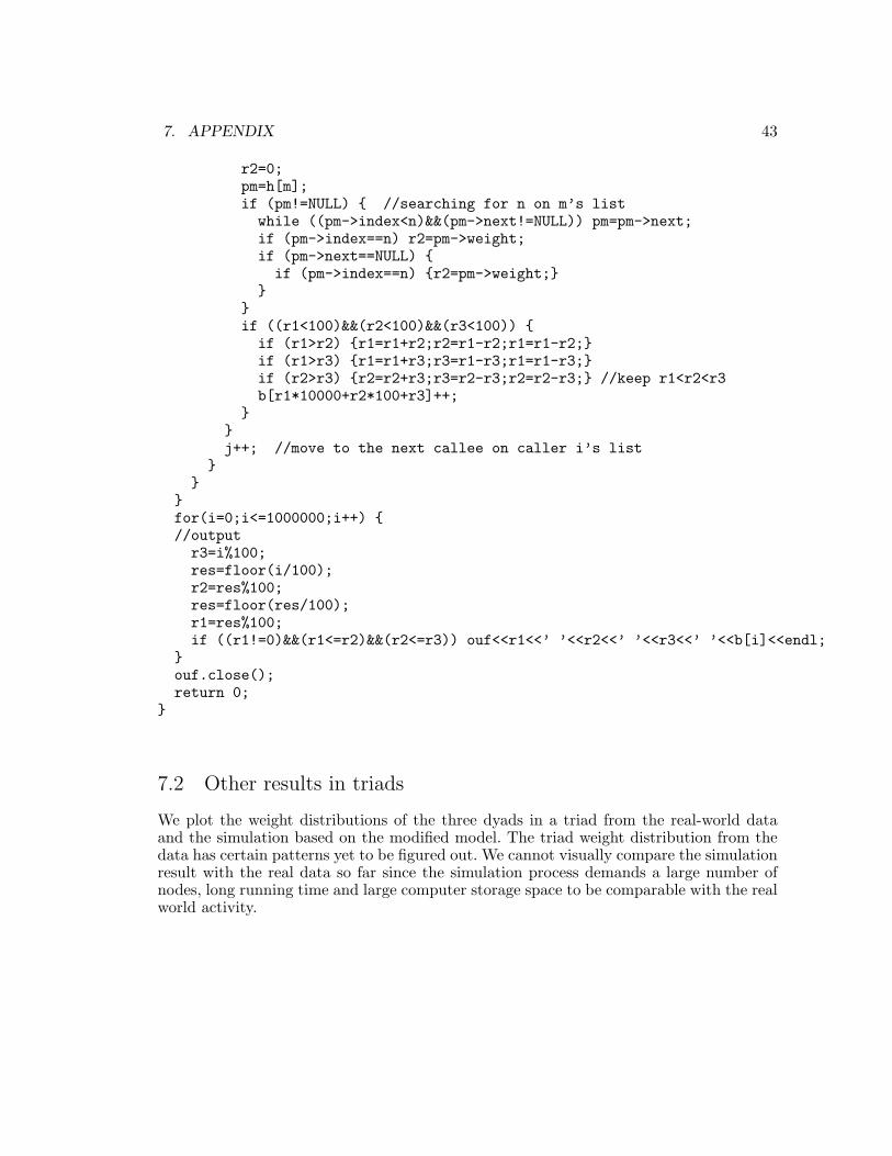
7.2 Other results in triads

We plot the weight distributions of the three dyads in a triad from the real-world dataand the simulation based on the modified model. The triad weight distribution from thedata has certain patterns yet to be figured out. We cannot visually compare the simulationresult with the real data so far since the simulation process demands a large number ofnodes, long running time and large computer storage space to be comparable with the realworld activity.

7. APPENDIX 44

Figure 7.2.1. Triad weight distribution from the data. The three axes represents the weightsof the three combining dyads. The color scale indicates log(frequency).

7. APPENDIX 45

Figure 7.2.2. Triad weight distribution from the simulation. The three axes represents theweights of the three combining dyads. The color scale indicates log(frequency).

Bibliography

[1] T. Antal, P. L. Krapivsky, and S. Redner, Dynamics of Social Balance on Networks,Physica E 72 (2005), 036–121.

[2] , Social balance on networks: The dynamics of friendship and enmity, PhysicaD 224 (2006), 130–136.

[3] A.-L. Barabasi and R. Albert, Emergence of Scaling in Random Networks, Science286 (1999), 509–512.

[4] A.-L. Barabasi, The Origin of Bursts and Heavy Tails in Human Dynamics, Nature435 (2005), 207–211.

[5] D. Cartwright and F. Harary, A generalization of Heider’s theory, Psychological Re-view 63 (1956), 277–292.

[6] Paul Erdos and Alfred Renyi, On Random Graphs, Publ. Math. Debrecen 6 (1959),290–297.

[7] Caroline Haythornthwaite, Social networks and Internet connectivity effects, Informa-tion Communication and Society 8 (2005), 125–147.

[8] F. Heider, Attitudes and cognitive organization, Journal of Psychology 21 (1946),107–112.

[9] Cesar Hidalgo and C. Rodriguez-Sickert, The dynamics of a mobile phone network,Physica A 387 (2008), 3017–3024.

[10] Barry D. Hughes, Random Walks and Random Environments, Oxford UniversityPress, USA, 1995.

[11] Renaud Lambiotte, Vincent D. Blondel, and Cristobald de Kerchove, Geographicaldispersal of mobile communication networks, Physica A 387 (2008), 5317–5325.

[12] Donald A. McQuarrie, Statistical Mechanics, University Science Books, Sausalito, CA,2000.

Bibliography 47

[13] R. Milo, S. Shen-Orr, S. Itzkovitz, N. Kashtan, D. Chklovskii, and U. Alon, NetworkMotifs: Simple Building Blocks of Complex Networks, Science 298 (2002), 824–827.

[14] J.P. Onnela, J. Saramaki, J. Hyvonen, G. Szabo, D. Lazer, K. Kaski, J. Kertesz,and A.-L. Barabasi, Structure and tie strengths in mobile communication networks,Proceedings of the National Academy of Sciences 104 (2007), 7332–7336.

[15] L.E. Reichl, A Modern Course in Statistical Physics, Wiley Publication, New York,NY, 1998.

[16] Stanley Wasserman and Katherine Faust, Social network analysis: methods and ap-plications, Cambridge University Press, New York, NY, 1994.

[17] Zhechao Zhou, Heterogeneous Patterns in Human Communication, Unpublished work(2008).

analysis of heterogeneous patterns and social dynamics in human

Documents