Analysis of Generalized Linear Mixed Models in the Agricultural and Natural Resources Sciences

GLM.indb 1 12/16/2011 10:28:34 AM

GLM.indb 2 12/16/2011 10:28:34 AM

Analysis of Generalized Linear Mixed Models in the Agricultural and Natural Resources Sciences

Edward E. Gbur, Walter W. Stroup, Kevin S. McCarter, Susan Durham,

Linda J. Young, Mary Christman, Mark West, and Matthew Kramer

Book and Multimedia Publishing CommitteeApril Ulery, ChairWarren Dick, ASA Editor-in-ChiefE. Charles Brummer, CSSA Editor-in-ChiefAndrew Sharpley, SSSA Editor-in-ChiefMary Savin, ASA RepresentativeMike Casler, CSSA RepresentativeDavid Clay, SSSA RepresentativeManaging Editor: Lisa Al-Amoodi

GLM.indb 3 12/16/2011 10:28:36 AM

Copyright © 2012 by American Society of Agronomy Soil Science Society of America Crop Science Society of America

ALL RIGHTS RESERVED. No part of this publication may be reproduced or transmitted in any form or by any means, electronic or mechanical, including photocopying, recording, or any information storage and retrieval system, without permission in writing from the publisher.

The views expressed in this publication represent those of the individual Editors and Authors. These views do not necessarily reflect endorsement by the Publisher(s). In addition, trade names are sometimes mentioned in this publication. No endorsement of these products by the Publisher(s) is intended, nor is any criticism implied of similar products not mentioned.

American Society of Agronomy Soil Science Society of America Crop Science Society of America, Inc.5585 Guilford Road, Madison, WI 53711-5801 USAhttps://www.agronomy.org/publications/books | www.SocietyStore.org

ISBN: 978-0-89118-182-8e-ISBN: 978-0-89118-183-5doi:10.2134/2012.generalized-linear-mixed-models

Library of Congress Control Number: 2011944082

Cover: Patricia Scullion Photo: Nathan Slaton, Univ. of Arkansas, Dep. of Crops, Soil, and Environmental Science

Printed in the United States of America.

GLM.indb 4 12/16/2011 10:28:36 AM

v

ContEntS

Foreword viiPreface ixAuthors xiConversion Factors for SI and Non-SI Units xiii

Chapter 1Introduction 1

1.1 Introduction 11.2 Generalized Linear Mixed Models 21.3 Historical Development 31.4 Objectives of this Book 5

Chapter 2Background 7

2.1 Introduction 72.2 Distributions used in Generalized Linear Modeling 72.3 Descriptions of the Distributions 102.4 Likelihood Based Approach to Estimation 152.5 Variations on Maximum Likelihood Estimation 182.6 Likelihood Based Approach to Hypothesis Testing 192.7 Computational Issues 222.8 Fixed, Random, and Mixed Models 242.9 The Design–Analysis of Variance–Generalized Linear Mixed Model Connection 252.10 Conditional versus Marginal Models 302.11 Software 30

Chapter 3Generalized Linear Models 35

3.1 Introduction 353.2 Inference in Generalized Linear Models 373.3 Diagnostics and Model Fit 463.4 Generalized Linear Modeling versus Transformations 52

Chapter 4Linear Mixed Models 59

4.1 Introduction 594.2 Estimation and Inference in Linear Mixed Models 604.3 Conditional and Marginal Models 614.4 Split Plot Experiments 674.5 Experiments Involving Repeated Measures 774.6 Selection of a Covariance Model 784.7 A Repeated Measures Example 804.8 Analysis of Covariance 884.9 Best Linear Unbiased Prediction 99

GLM.indb 5 12/16/2011 10:28:36 AM

vi

Chapter 5Generalized Linear Mixed Models 109

5.1 Introduction 1095.2 Estimation and Inference in Generalized Linear Mixed Models 1105.3 Conditional and Marginal Models 1115.4 Three Simple Examples 1255.5 Over-Dispersion in Generalized Linear Mixed Models 1495.6 Over-Dispersion from an Incorrectly Specified Distribution 1515.7 Over-Dispersion from an Incorrect Linear Predictor 1605.8 Experiments Involving Repeated Measures 1675.9 Inference Issues for Repeated Measures Generalized Linear Mixed Models 1815.10 Multinomial Data 184

Chapter 6More Complex Examples 199

6.1 Introduction 1996.2 Repeated Measures in Time and Space 1996.3 Analysis of a Precision Agriculture Experiment 210

Chapter 7Designing Experiments 237

7.1 Introduction 2377.2 Power and Precision 2387.3 Power and Precision Analyses for Generalized Linear Mixed Models 2397.4 Methods of Determining Power and Precision 2417.5 Implementation of the Probability Distribution Method 2437.6 A Factorial Experiment with Different Design Options 2507.7 A Multi-location Experiment with a Binomial Response Variable 2557.8 A Split Plot Revisited with a Count as the Response Variable 2627.9 Summary and Conclusions 268

Chapter 8Parting thoughts and Future Directions 271

8.1 The Old Standard Statistical Practice 2718.2 The New Standard 2728.3 The Challenge to Adapt 274

Index 277

GLM.indb 6 12/16/2011 10:28:36 AM

vii

ForEWorD

Analysis of Generalized Linear Mixed Models in the Agricultural and Natural Resources Sciences is an excellent resource book for students and professionals alike. This book explains the use of generalized linear mixed models which are applicable to students of agricultural and natural resource sciences. The strength of the book is the available examples and statistical analysis system (SAS) code used for analy-sis. These “real life” examples provide the reader with the examples needed to understand and use generalized linear mixed models for their own analysis of experimental data. This book, published by the American Society of Agronomy, Crop Science Society of America, and the Soil Science Society of America, will be valuable as its practical nature will help scientists in training as well as practic-ing scientists. The goal of the three Societies is to provide educational material to advance the profession. This book helps meet this goal.

Chuck rice, 2011 Soil Science Society of America Presidentnewell Kitchen, 2011 American Society of Agronomy PresidentMaria Gallo, 2011 Crop Science Society of America President

GLM.indb 7 12/16/2011 10:28:36 AM

GLM.indb 8 12/16/2011 10:28:36 AM

ix

Pr E FaC E

The authors of this book are participants in the Multi-state Project NCCC-170 “Research Advances in Agricultural Statistics” under the auspices of the North Central Region Agricultural Experiment Station Directors. Project members are statisticians from land grant universities, USDA-ARS, and industry who are inter-ested in agricultural and natural resource applications of statistics. The project has been in existence since 1991. We consider this book as part of the educational outreach activities of our group. Readers interested in NCCC-170 activities can access the project website through a link on the National Information Manage-ment and Support System (NIMSS).

Traditional statistical methods have been developed primarily for normally distributed data. Generalized linear mixed models extend normal theory linear mixed models to include a broad class of distributions, including those com-monly used for counts, proportions, and skewed distributions. With the advent of software for implementing generalized linear mixed models, we have found researchers increasingly interested in using these models, but it is “easier said than done.” Our goal is to help those who have worked with linear mixed models to begin moving toward generalized linear mixed models. The benefits and chal-lenges are discussed from a practitioner’s viewpoint. Although some readers will feel confident in fitting these models after having worked through the examples, most will probably use this book to become aware of the potential these models promise and then work with a professional statistician for full implementation, at least for their first few applications.

The original purpose of this book was as an educational outreach effort to the agricultural and natural resources research community. This remains as its primary purpose, but in the process of preparing this work, each of us found it to be a wonderful professional development experience. Each of the authors under-stood some aspects of generalized linear mixed models well, but no one “knew it all.” By pooling our combined understanding and discussing different perspec-tives, we each have benefitted greatly. As a consequence, those with whom we consult will benefit from this work as well.

We wish to thank our reviewers Bruce Craig, Michael Guttery, and Margaret Nemeth for their careful reviews and many helpful comments. Jeff Velie con-structed many of the graphs that were not automatically generated by SAS (SAS Institute, Cary, NC). Thank you, Jeff. We are grateful to all of the scientists who so willingly and graciously shared their research data with us for use as examples.

Edward E. Gbur, Walter W. Stroup, Kevin S. McCarter, Susan Durham, Linda J. Young, Mary Christman, Mark West, and Matthew Kramer

GLM.indb 9 12/16/2011 10:28:36 AM

GLM.indb 10 12/16/2011 10:28:36 AM

xi

authorS

Edward Gbur is currently Professor and Director of the Agricultural Statistics Laboratory at the University of Arkansas. Previously he was on the faculty in the Statistics Department at Texas A&M University and was a Mathematical Statistician in the Statistical Research Division at the Census Bureau. He received a Ph.D. in Statistics from The Ohio State University. He is a member and Fellow of the American Statistical Association and a member of the International Biometric Society and the Institute of Mathematical Statistics. His current research interests include experimental design, generalized linear mixed models, stochastic modeling, and agricultural applications of statistics.

Walter Stroup is Professor of Statistics at the University of Nebraska, Lincoln. After receiving his Ph.D. in Statistics from the University of Kentucky in 1979, he joined the Biometry faculty at Nebraska’s Institute of Agriculture and Natural Resources. He served as teacher, researcher, and consultant until becoming department chair in 2001. In 2003, Biometry was incorporated into a new Department of Statistics at UNL; Walt served as chair from its founding through 2010. He is co-author of SAS for Mixed Models and SAS for Linear Models. He is a member of the International Biometric Society, American Association for the Advancement of Science, and a member and Fellow of the American Statistical Association. His interests include design of experiments and statistical modeling.

Kevin S. McCarter is a faculty member in the Department of Experimental Statistics at Louisiana State University. He earned the Bachelors degree with majors in Mathematics and Computer Information Systems from Washburn University and the Masters and Ph.D. degrees in Statistics from Kansas State University. He has industry experience as an IT professional in banking, accounting, and health care, and as a biostatistician in the pharmaceutical industry. His dissertation research was in the area of survival analysis. His current research interests include predictive modeling, developing and assessing statistical methodology, and applying generalized linear mixed modeling techniques. He has collaborated with researchers from a wide variety of fields, including agriculture, biology, education, medicine, and psychology.

Susan Durham is a statistical consultant at Utah State University, collaborating with faculty and graduate students in the Ecology Center, Biology Department, and College of Natural Resources. She earned a Bachelors degree in Zoology at Oklahoma State University and a Masters degree in Applied Statistics at Utah State University. Her interests cover the broad range of research problems that have been brought to her as a statistical consultant.

GLM.indb 11 12/16/2011 10:28:36 AM

xii

Mary Christman is currently the lead statistical consultant with MCC Statistical Consulting LLC, which provides statistical expertise for environmental and ecological problems. She is also courtesy professor at the University of Florida. She was on the faculty at University of Florida, University of Maryland, and American University after receiving her Ph.D. in statistics from George Washington University. She is a member of several organizations, including the American Statistical Association, the International Environmetrics Society, and the American Association for the Advancement of Science. She received the 2004 Distinguished Achievement Award from the Section on Statistics and the Environment of the American Statistical Association. Her current research interests include linear and non-linear modeling in the presence of correlated error terms, sampling and experimental design, and statistical methodology for ecological and environmental research.

Linda J. Young is Professor of Statistics at the University of Florida. She completed her Ph.D. in Statistics at Oklahoma State University and has previously served on the faculties of Oklahoma State University and the University of Nebraska, Lincoln. Linda has served the profession in a variety of capacities, including President of the Eastern North American Region of the International Biometric Society, Treasurer of the International Biometric Society, Vice-President of the American Statistical Association, and Chair of the Committee of Presidents of Statistical Societies. She has co-authored two books and has more than 100 refereed publications. She is a fellow of the American Association for the Advancement of Science, a fellow of the American Statistical Association, and an elected member of the International Statistical Institute. Her research interests include spatial statistics and statistical modeling.

Mark West is a statistician for the USDA-Agricultural Research Service. He received his Ph.D. in Applied Statistics from the University of Alabama in 1989 and has been a statistical consultant in agriculture research ever since beginning his professional career at Auburn University in 1989. His interests include experimental design, statistical computing, computer intensive methods, and generalized linear mixed models.

Matt Kramer is a statistician in the mid-Atlantic area (Beltsville, MD) of the USDA-Agricultural Research Service, where he has worked since 1999. Prior to that, he spent eight years at the Census Bureau in the Statistical Research Division (time series and small area estimation). He received a Masters and Ph.D. from the University of Tennessee. His interests are in basic biological and ecological statistical applications.

GLM.indb 12 12/16/2011 10:28:37 AM

xiii

Co n v E r S I o n FaC to r S Fo r S I a n D n o n -S I u n I tS

To convert Column 1 into Column 2 multiply by

Column 1 SI unit

Column 2 non-SI unit

To convert Column 2 into Column 1 multiply by

Length0.621 kilometer, km (103 m) mile, mi 1.6091.094 meter, m yard, yd 0.9143.28 meter, m foot, ft 0.3041.0 micrometer, µm (10−6 m) micron, µ 1.03.94 × 10−2 millimeter, mm (10−3 m) inch, in 25.410 nanometer, nm (10−9 m) Angstrom, Å 0.1

area2.47 hectare, ha acre 0.405247 square kilometer, km2 (103 m)2 acre 4.05 × 10−3

0.386 square kilometer, km2 (103 m)2 square mile, mi2 2.5902.47 × 10−4 square meter, m2 acre 4.05 × 103

10.76 square meter, m2 square foot, ft2 9.29 × 10−2

1.55 × 10−3 square millimeter, mm2 (10−3 m)2

square inch, in2 645

volume9.73 × 10−3 cubic meter, m3 acre-inch 102.835.3 cubic meter, m3 cubic foot, ft3 2.83 × 10−2

6.10 × 104 cubic meter, m3 cubic inch, in3 1.64 × 10−5

2.84 × 10−2 liter, L (10−3 m3) bushel, bu 35.241.057 liter, L (10−3 m3) quart (liquid), qt 0.9463.53 × 10−2 liter, L (10−3 m3) cubic foot, ft3 28.30.265 liter, L (10−3 m3) gallon 3.7833.78 liter, L (10−3 m3) ounce (fluid), oz 2.96 × 10−2

2.11 liter, L (10−3 m3) pint (fluid), pt 0.473

Mass2.20 × 10−3 gram, g (10−3 kg) pound, lb 4543.52 × 10−2 gram, g (10−3 kg) ounce (avdp), oz 28.42.205 kilogram, kg pound, lb 0.4540.01 kilogram, kg quintal (metric), q 100

1.10 × 10−3 kilogram, kg ton (2000 lb), ton 9071.102 megagram, Mg (tonne) ton (U.S.), ton 0.9071.102 tonne, t ton (U.S.), ton 0.907

Yield and rate0.893 kilogram per hectare, kg ha−1 pound per acre, lb acre−1 1.127.77 × 10−2 kilogram per cubic meter,

kg m−3pound per bushel, lb bu−1 12.87

1.49 × 10−2 kilogram per hectare, kg ha−1 bushel per acre, 60 lb 67.191.59 × 10−2 kilogram per hectare, kg ha−1 bushel per acre, 56 lb 62.71

continued

GLM.indb 13 12/16/2011 10:28:37 AM

xiv

To convert Column 1 into Column 2 multiply by

Column 1 SI unit

Column 2 non-SI unit

To convert Column 2 into Column 1 multiply by

1.86 × 10−2 kilogram per hectare, kg ha−1 bushel per acre, 48 lb 53.750.107 liter per hectare, L ha−1 gallon per acre 9.35893 tonne per hectare, t ha−1 pound per acre, lb acre−1 1.12 × 10−3

893 megagram per hectare, Mg ha−1 pound per acre, lb acre−1 1.12 × 10−3

0.446 megagram per hectare, Mg ha−1 ton (2000 lb) per acre, ton acre−1 2.242.24 meter per second, m s−1 mile per hour 0.447

Specific Surface10 square meter per kilogram,

m2 kg−1square centimeter per gram,

cm2 g−10.1

1000 square meter per kilogram, m2 kg−1

square millimeter per gram, mm2 g−1

0.001

Density1.00 megagram per cubic meter,

Mg m−3gram per cubic centimeter, g cm−3 1.00

Pressure9.90 megapascal, MPa (106 Pa) atmosphere 0.10110 megapascal, MPa (106 Pa) bar 0.12.09 × 10−2 pascal, Pa pound per square foot, lb ft−2 47.91.45 × 10−4 pascal, Pa pound per square inch, lb in−2 6.90 × 103

temperature1.00 (K − 273) kelvin, K Celsius, °C 1.00 (°C + 273)(9/5 °C) + 32 Celsius, °C Fahrenheit, °F 5/9 (°F − 32)

Energy, Work, Quantity of heat9.52 × 10−4 joule, J British thermal unit, Btu 1.05 × 103

0.239 joule, J calorie, cal 4.19107 joule, J erg 10−7

0.735 joule, J foot-pound 1.362.387 × 10−5 joule per square meter, J m−2 calorie per square centimeter

(langley)4.19 × 104

105 newton, N dyne 10−5

1.43 × 10−3 watt per square meter, W m−2 calorie per square centimeter minute (irradiance), cal cm−2 min−1

698

transpiration and Photosynthesis3.60 × 10−2 milligram per square meter

second, mg m−2 s−1gram per square decimeter hour,

g dm−2 h−127.8

5.56 × 10−3 milligram (H2O) per square meter second, mg m−2 s−1

micromole (H2O) per square centimeter second, µmol cm−2 s−1

180

10−4 milligram per square meter second, mg m−2 s−1

milligram per square centimeter second, mg cm−2 s−1

104

35.97 milligram per square meter second, mg m−2 s−1

milligram per square decimeter hour, mg dm−2 h−1

2.78 × 10−2

continued

GLM.indb 14 12/16/2011 10:28:37 AM

xv

To convert Column 1 into Column 2 multiply by

Column 1 SI unit

Column 2 non-SI unit

To convert Column 2 into Column 1 multiply by

Plane angle57.3 radian, rad degrees (angle), ° 1.75 × 10−2

Electrical Conductivity, Electricity, and Magnetism10 siemen per meter, S m−1 millimho per centimeter,

mmho cm−10.1

104 tesla, T gauss, G 10−4

Water Measurement9.73 × 10−3 cubic meter, m3 acre-inch, acre-in 102.89.81 × 10−3 cubic meter per hour, m3 h−1 cubic foot per second, ft3 s−1 101.94.40 cubic meter per hour, m3 h−1 U.S. gallon per minute,

gal min−10.227

8.11 hectare meter, ha m acre-foot, acre-ft 0.12397.28 hectare meter, ha m acre-inch, acre-in 1.03 × 10−2

8.1 × 10−2 hectare centimeter, ha cm acre-foot, acre-ft 12.33

Concentration1 centimole per kilogram, cmol kg−1 milliequivalent per 100 grams,

meq 100 g−11

0.1 gram per kilogram, g kg−1 percent, % 101 milligram per kilogram, mg kg−1 parts per million, ppm 1

radioactivity2.7 × 10−11 becquerel, Bq curie, Ci 3.7 × 1010

2.7 × 10−2 becquerel per kilogram, Bq kg−1 picocurie per gram, pCi g−1 37100 gray, Gy (absorbed dose) rad, rd 0.01100 sievert, Sv (equivalent dose) rem (roentgen equivalent man) 0.01

Plant nutrient ConversionElemental Oxide

2.29 P P2O5 0.4371.20 K K2O 0.8301.39 Ca CaO 0.7151.66 Mg MgO 0.602

GLM.indb 15 12/16/2011 10:28:37 AM

GLM.indb 16 12/16/2011 10:28:37 AM

1

doi:10.2134/2012.generalized-linear-mixed-models.c1

Copyright © 2012 American Society of Agronomy, Crop Science Society of America, and Soil Science Society of America5585 Guilford Road, Madison, WI 53711-5801, USA.

Analysis of Generalized Linear Mixed Models in the Agricultural and Natural Resources SciencesEdward E. Gbur, Walter W. Stroup, Kevin S. McCarter, Susan Durham, Linda J. Young, Mary Christman, Mark West, and Matthew Kramer

ChaPtEr 1

INtRoductIoN

1.1 IntroDuCtIon

Over the past generation, dramatic advances have occurred in statistical meth-odology, many of which are relevant to research in the agricultural and natural resources sciences. These include more theoretically sound approaches to the analysis of spatial data; data taken over time; data involving discrete, categorical, or continuous but non-normal response variables; multi-location and/or multi-year data; complex split-plot and repeated measures data; and genomic data such as data from microarray and quantitative genetics studies. The development of generalized linear mixed models has brought together these apparently disparate problems under a coherent, unified theory. The development of increasingly user friendly statistical software has made the application of this methodology acces-sible to applied researchers.

The accessibility of generalized linear mixed model software has coincided with a time of change in the research community. Research budgets have been tight-ening for several years, and there is every reason to expect this trend to continue for the foreseeable future. The focus of research in the agricultural sciences has been shifting as the nation and the world face new problems motivated by the need for clean and renewable energy, management of limited natural resources, environmen-tal stress, the need for crop diversification, the advent of precision agriculture, safety dilemmas, and the need for risk assessment associated with issues such as geneti-cally modified crops. New technologies for obtaining data offer new and important possibilities but often are not suited for design and analysis using conventional approaches developed decades ago. With this rapid development comes the lack of accepted guidelines for how such data should be handled.

Researchers need more efficient ways to conduct research to obtain useable information with the limited budgets they have. At the same time, they need ways to meaningfully analyze and understand response variables that are very differ-ent from those covered in “traditional” statistical methodology. Generalized linear mixed models allow more versatile and informative analysis in these situations and, in the process, provide the tools to facilitate experimental designs tailored to

GLM.indb 1 12/16/2011 10:28:37 AM

2 CHAPTER 1

the needs of particular studies. Such designs are often quite different from conven-tional experimental designs. Thus, generalized linear mixed models provide an opportunity for a comprehensive rethinking of statistical practice in agricultural and natural resources research. This book provides a practical introductory guide to this topic.

1.2 GEnEraLIzED LInEar MIxED MoDELS

In introductory statistical methods courses taken by nearly every aspiring agri-cultural scientist in graduate school, statistical analysis is presented in some way, shape, or form as an attempt to make inferences on observations that are the sum of “explanatory” components and “random” components. In designed experi-ments and quasi-experiments (i.e., studies structured as closely as possible to de-signed experiments), “explanatory” means treatment effect and “random” means residual or random error. Thus, the formula

observed response = explanatory + random

expresses the basic building blocks of statistical methodology. This simple break-down is necessarily elaborated into

observed response = treatment + design effects + error

where design effects include blocks and covariates. The observed response is inevitably interpreted as having a normal distribution and analysis of variance (ANOVA), regression, and analysis of covariance are presented as the primary methods of analysis. In contemporary statistics, such models are collectively referred to as linear models. In simple cases, a binomial distribution is consid-ered for the response variable leading to logit analysis and logistic regression. Occasionally probit analysis is considered as well.

In contrast, consider what the contemporary researcher actually faces. Table 1–1 shows the types of observed response variables and explanatory model compo-nents that researchers are likely to encounter. Note that “conventional” statistical methodology taught in introductory statistics courses and widely considered as

“standard statistical analysis” in agricultural research and journal publication is confined to the first row and occasionally the second row in the table. Obviously, the range of methods considered “standard” is woefully inadequate given the range of possibilities now faced by contemporary researchers.

This inadequacy has a threefold impact on potential advances in agricultural and applied research. First, it limits the types of analyses that researchers (and journal editors) will consider, resulting in cases where “standard methods” are a mismatch between the observed response and an explanatory model. Second, it limits researchers’ imaginations when planning studies, for example through a lack of awareness of alternative types of response variables that contemporary statistical methods can handle. Finally, it limits the efficiency of experiments in that traditional designs, while optimized for normal distribution based ANOVA

GLM.indb 2 12/16/2011 10:28:37 AM

INTRODUCTION 3

and regression, often are not well suited to the majority of the response variable–explanatory model combinations in Table 1–1.

Two major advances in statistical theory and methodology that occurred in the last half of the 20th century were the development of linear mixed models and gen-eralized linear models. Mixed models incorporate random effects and correlated errors; that is, they deal with all four columns of explanatory model components in Table 1–1. Generalized linear models accommodate a large class of probability distributions of the response; that is, they deal with the response variable column in the table. The combination of mixed and generalized linear models, namely gen-eralized linear mixed models, addresses the entire range of options for the response variable and explanatory model components (i.e., with all 20 combinations in Table 1 –1). Generalized linear mixed models represent the primary focus of this book.

1.3 hIStorICaL DEvELoPMEnt

Seal (1967) traced the origin of fixed effects models back to the development of least squares by Legendre in 1806 and Gauss in 1809, both in the context of prob-lems in astronomy. It is less well known that the origin of random effects models can be ascribed to astronomy problems as well. Scheffé (1956) attributed early use

taBLE 1–1. Statistical model scenarios corresponding to combinations of types of observed responses and explanatory model components.

type of response variable

Examples of distributions

Explanatory model components

Fixed effects

Random effectscorrelated

errorscategorical continuous

Continuous,unbounded

values,symmetric

normal ANOVA†,‡,§,¶ regression †,‡,§,¶

split plot ANOVA‡,¶ —‡,¶

Categorical binomial, multinomial

logit analysis§,¶

logistic regression §,¶ —¶ —¶

Count Poisson, negative binomial

log-linear model §,¶

Poisson regression §,¶ —¶ —¶

Continuous,non-negative

values

lognormal, gamma, beta —§,¶ —§,¶ —¶ —¶

Time to eventexponential,

gamma, geometric

—§,¶ —§,¶ —¶ —¶

† Linear model scenarios are limited to the first two cells in the first row of the table.‡ Linear mixed model scenarios are limited to first row of the table.§ Generalized linear model scenarios are limited to first two columns of the table.¶ Generalized linear mixed model scenarios cover all cells shown in the table.

GLM.indb 3 12/16/2011 10:28:38 AM

4 CHAPTER 1

of random effects to Airy in an 1861 publication. It was not until nearly 60 years later that Fisher (1918) formally introduced the terms variance and analysis of vari-ance and utilized random effects models.

Fisher’s 1935 first edition of The Design of Experiments implicitly discusses mixed models (Fisher, 1935). Scheffé (1956) attributed the first explicit expression of a mixed model equation to Jackson (1939). Yates (1940) developed methods to recover inter-block information in block designs that are equivalent to mixed model analysis with random blocks. Eisenhart (1947) formally identified random, fixed, and mixed models. Henderson (1953) was the first to explicitly use mixed model methodology for animal genetics studies. Harville (1976, 1977) published the formal overall theory of mixed models.

Although analyses of special cases of non-normally distributed responses such as probit analysis (Bliss, 1935) and logit analysis (Berkson, 1944) existed in the con-text of bioassays, standard statistical methods textbooks such as Steel et al. (1997) and Snedecor and Cochran (1989) dealt with the general problem of non-normal-ity through the use of transformations. The ultimate purpose of transformations such as the logarithm, arcsine, and square root was to enable the researcher to obtain approximate analyses using the standard normal theory methods. Box and Cox (1964) proposed a general class of transformations that include the above as special cases. They too have been applied to allow use of normal theory methods.

Nelder and Wedderburn (1972) articulated a comprehensive theory of linear models with non-normally distributed response variables. They assumed that the response distribution belonged to the exponential family. This family of probabil-ity distributions contains a diverse set of discrete and continuous distributions, including all of those listed in Table 1–1. The models were referred to as general-ized linear models (not to be confused with general linear models which has been used in reference to normally distributed responses only). Using the concept of quasi-likelihood, Wedderburn (1974) extended applicability of generalized linear models to certain situations where the distribution cannot be specified exactly. In these cases, if the observations are independent or uncorrelated and the form of the mean/variance ratio can be specified, it is possible to fit the model and obtain results similar to those which would have been obtained if the distribution had been known. The monograph by McCullagh and Nelder (1989) brought general-ized linear models to the attention of the broader statistical community and with it, the beginning of research on the addition of random effects to these models—the development of generalized linear mixed models.

By 1992 the conceptual development of linear models through and including generalized linear mixed models had been accomplished, but the computational capabilities lagged. The first usable software for generalized linear models appeared in the mid 1980s, the first software for linear mixed models in the 1990s, and the first truly usable software for generalized linear mixed models appeared in the mid 2000s. Typically there is a 5- to 10-year lag between the introduction of the software and the complete appreciation of the practical aspects of data analy-ses using these models.

GLM.indb 4 12/16/2011 10:28:38 AM

INTRODUCTION 5

1.4 oBJECtIvES oF thIS BooK

Our purpose in writing this book is to lead practitioners gently through the basic concepts and currently available methods needed to analyze data that can be mod-eled as a generalized linear mixed model. These concepts and methods require a change in mindset from normal theory linear models that will be elaborated on at various points in the following chapters. As with all new methodology, there is a learning curve associated with this material and it is important that the theory be understood at least at some intuitive level. We assume that the reader is familiar with the corresponding standard techniques for normally distributed responses and has some experience using these methods with statistical software such as SAS (SAS Institute, Cary, NC) or R (CRAN, www.r-project.org [verified 27 Sept. 2011]). While it is necessary to use matrix language in some places, we have at-tempted to keep the mathematical level as accessible as possible for the reader. We believe that readers who find the mathematics too difficult will still find much of this book useful. Numerical examples have been included throughout to illustrate the concepts. The emphasis in these examples is on illustration of the methodol-ogy and not on subject matter results.

Chapter 2 presents background on the exponential family of probability distributions and the likelihood based statistical inference methods used in the analysis of generalized linear mixed models. Chapter 3 introduces generalized linear models containing only fixed effects. Random effects and the corresponding mixed models having normally distributed responses are the subjects of Chapter 4. Chapter 5 begins the discussion of generalized linear mixed models. In Chapter 6, detailed analyses of two more complex examples are presented. Finally we turn to design issues in Chapter 7, where our purpose is to provide examples of a meth-odology that allows the researcher to plan studies involving generalized linear mixed models that directly address his/her primary objectives efficiently. Chapter 8 contains final remarks.

This book represents a first effort to describe the analysis of generalized linear mixed models in the context of applications in the agricultural sciences. We are still in that early period following the introduction of software capable of fitting these models, and there are some unresolved issues concerning various aspects of working with these methods. As examples are introduced in the following chap-ters, we will note some of the issues that a data analyst is likely to encounter and will provide advice as to the best current thoughts on how to handle them. One recurring theme that readers will notice, especially in Chapter 5, is that comput-ing software defaults often must be overridden. With increased capability comes increased complexity. It is unrealistic to expect one-size-fits-all defaults for gener-alized linear mixed model software. As these situations arise in this book, we will explain what to do and why. The benefit for the additional effort is more accurate analysis and higher quality information per research dollar.

GLM.indb 5 12/16/2011 10:28:38 AM

6 CHAPTER 1

rEFErEnCES CItEDBerkson, J. 1944. Application of the logistic function to bio-assay. J. Am. Stat. Assoc.

39:357–365. doi:10.2307/2280041Bliss, C.A. 1935. The calculation of the dose-mortality curve. Ann. Appl. Biol. 22:134–

167. doi:10.1111/j.1744-7348.1935.tb07713.xBox, G.E.P., and D.R. Cox. 1964. An analysis of transformations. J. R. Stat. Soc. Ser. B

(Methodological) 26:211–252.Eisenhart, C. 1947. The assumptions underlying the analysis of variance. Biometrics

3:1–21. doi:10.2307/3001534Fisher, R.A. 1918. The correlation between relatives on the supposition of Mendelian

inheritance. Trans. R. Soc. Edinb. 52:399–433.Fisher, R.A. 1935. The design of experiments. Oliver and Boyd, Edinburgh.Harville, D.A. 1976. Confidence intervals and sets for linear combinations of fixed and

random effects. Biometrics 32:403–407. doi:10.2307/2529507Harville, D.A. 1977. Maximum likelihood approaches to variance component

estimation and to related problems. J. Am. Stat. Assoc. 72:320–338. doi:10.2307/2286796

Henderson, C.R. 1953. Estimation of variance and covariance components. Biometrics 9:226–252. doi:10.2307/3001853

Jackson, R.W.B. 1939. The reliability of mental tests. Br. J. Psychol. 29:267–287.McCullagh, P., and J.A. Nelder. 1989. Generalized linear models. 2nd ed. Chapman and

Hall, New York.Nelder, J.A., and R.W.M. Wedderburn. 1972. Generalized linear models. J. R. Stat. Soc.

Ser. A (General) 135:370–384. doi:10.2307/2344614Scheffé, H. 1956. Alternative models for the analysis of variance. Ann. Math. Stat.

27:251–271. doi:10.1214/aoms/1177728258Seal, H.L. 1967. The historical development of the Gauss linear model. Biometrika

54:1–24.Snedecor, G.W., and W.G. Cochran. 1989. Statistical methods. 8th ed. Iowa State Univ.

Press, Ames, IA.Steel, R.G.D., J.H. Torrie, and D.A. Dickey. 1997. Principles and procedures of statistics:

A biometrical approach. 3rd ed. McGraw-Hill, New York.Wedderburn, R.W.M. 1974. Quasi-likelihood functions, generalized linear models and

the Gauss-Newton method. Biometrika 61:439–447.Yates, F. 1940. The recovery of interblock information in balanced incomplete block

designs. Ann. Eugen. 10:317–325. doi:10.1111/j.1469-1809.1940.tb02257.x

GLM.indb 6 12/16/2011 10:28:38 AM

7

doi:10.2134/2012.generalized-linear-mixed-models.c2

Copyright © 2012 American Society of Agronomy, Crop Science Society of America, and Soil Science Society of America5585 Guilford Road, Madison, WI 53711-5801, USA.

Analysis of Generalized Linear Mixed Models in the Agricultural and Natural Resources SciencesEdward E. Gbur, Walter W. Stroup, Kevin S. McCarter, Susan Durham, Linda J. Young, Mary Christman, Mark West, and Matthew Kramer

ChaPtEr 2

BAckGRouNd

2.1 IntroDuCtIon

This chapter provides background material necessary for an understanding of generalized linear mixed models. It includes a description of the exponential fam-ily of probability distributions and several other commonly used distributions in generalized linear models. An important characteristic that distinguishes a non-normal distribution in this family from the normal distribution is that its variance is a function of its mean. As a consequence, these models have heteroscedastic variance structures because the variance changes as the mean changes. A familiar example of this is the binomial distribution based on n independent trials, each having success probability p. The mean is m = np, and the variance is np(1 − p) = m(1 − m/n).

The method of least squares has been commonly used as the basis for esti-mation and statistical inference in linear models where the response is normally distributed. As an estimation method, least squares is a mathematical method for minimizing the sum of squared errors that does not depend on the probability distribution of the response. While suitable for fixed effects models with normally distributed data, least squares does not generalize well to models with random effects, non-normal data, or both. Likelihood based procedures provide an alter-native approach that incorporates the probability distribution of the response into parameter estimation as well as inference. Inference for mixed and generalized lin-ear models is based on a likelihood approach described in Sections 2.4 through 2.7.

The basic concepts of fixed and random effects and the formulation of mixed models are reviewed in Sections 2.8 through 2.10. The final section of this chapter discusses available software.

2.2 DIStrIButIonS uSED In GEnEraLIzED LInEar MoDELInG

Probability distributions that can be written in the form

( ) ( ) ( )( | , ) exp ( , )( )

t y v A vf y v h ya

é ùh -ê úf = + fê úfë û

GLM.indb 7 12/16/2011 10:28:38 AM

8 CHAPTER 2

are said to be members of the exponential family of distributions. The function f(y | v,f) is the probability distribution of the response variable Y given v and f, the location and scale parameters, respectively. The functions t(×), h(×), A(×), a(×), and h(×) depend on either the data, the parameters or both as indicated. The quan-tity h(ν) is known as the natural parameter or canonical form of the parameter. As will be seen in Chapter 3, the canonical parameter q = h(v) plays an important role in generalized linear models. The mean and variance of the random variable Y can be shown to be a function of the parameter v and hence, of q. As a result, for members of the one parameter exponential family, the probability distribution of Y determines both the canonical form of the parameter and the form of the vari-ance as a function of v.

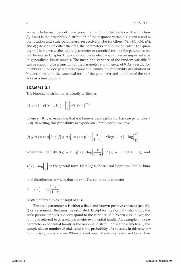
ExaMPLE 2.1

The binomial distribution is usually written as

( ) ( ) ( )| | 1 n yynf y P Y y

y-æ ö÷ç ÷p = = p = p - pç ÷ç ÷÷çè ø

where y = 0,..., n. Assuming that n is known, the distribution has one parameter p (= v). Rewriting this probability in exponential family form, we have

( ) ( ){ } ( )| exp log | exp log log 1 log

1n

f y f y y ny

é ùæ öæ öp ÷ç÷çê úé ù ÷÷p = p = + -p + çç ÷÷ê ú ê úçë û ç ÷÷ ÷ç- pè ø è øê úë û

where we identify t(y) = y, ( ) log1

æ öp ÷ç ÷h p = ç ÷ç ÷- pè ø, A(p) = −n log(1 − p), and

( ) logn

h yy

æ ö÷ç ÷= ç ÷ç ÷÷çè ø in the general form. Here log is the natural logarithm. For the bino-

mial distribution, f = 1, so that a(f) = 1. The canonical parameter

( ) log1

æ öp ÷ç ÷q = h p = ç ÷ç ÷- pè ø

is often referred to as the logit of p. ■The scale parameter f is either a fixed and known positive constant (usually

1) or a parameter that must be estimated. Except for the normal distribution, the scale parameter does not correspond to the variance of Y. When f is known, the family is referred to as a one parameter exponential family. An example of a one-parameter exponential family is the binomial distribution with parameters n, the sample size or number of trials, and p, the probability of a success. In this case, f = 1, and n is typically known. When f is unknown, the family is referred to as a two

GLM.indb 8 12/16/2011 10:28:38 AM

BACKGROUND 9

parameter exponential family. An example of a two parameter exponential family is the normal distribution where, for generalized linear model purposes, v is the mean and f is the variance. Another example of a two parameter distribution is the gamma distribution where v is the mean and fv2 is the variance. Note that for the normal distribution the mean and variance are distinct parameters, but for the gamma distribution the variance depends on both the mean and the scale param-eters. Other distributions in which the variance depends on both the mean and scale parameters include the beta and negative binomial distributions (Section 2.3).

ExaMPLE 2.2

The normal distribution with mean m and variance s2 is usually written as

( ) ( )2222

1 1| , exp22

f y yé ùê úm s = - - mê úsë ûps

where y is any real number. Assuming that both m and s2 are unknown parameters, v = m and f = s2. Rewriting f(y | m, s2) in exponential family form, we have

( )2 2 2 22 2 2

1 1 1| , exp log 22 2

f y y yé ùæ ö÷ê úçm s = - ps - + m- m÷ç ÷çê úè ø s s së û

and we identify t(y) = y, h(m) = m, a(s2) = s2, A(m) = m2/2, and

( )2 2 2 2( , ) log 2 2h y yæ ö÷çs =- ps - s÷ç ÷çè ø. ■

Table 2–1 contains a list of probability distributions belonging to the expo-nential family that are commonly used in generalized linear models. In addition to the exponential family of distributions, several other probability distributions are available for generalized linear modeling. These include the negative binomial, the non-central t, and the multinomial distributions (Table 2–2). If d is known, the negative binomial belongs to the one parameter exponential family. The multino-mial distribution generalizes the binomial distribution to more than two mutually exclusive and exhaustive categories. The categories can be either nominal (unor-dered) or ordinal (ordered or ranked).

GLM.indb 9 12/16/2011 10:28:38 AM

10 CHAPTER 2

2.3 DESCrIPtIonS oF thE DIStrIButIonS

In this section, each of the non-normal distributions commonly used in general-ized linear models is described, and examples of possible applications are given.

BEta

A random variable distributed according to the beta distribution is continuous, tak-ing on values within the range 0 to 1. Its mean is m, and its variance, m(1 − m)/(1 + f), depends on the mean (Table 2–1). The beta distribution is useful for modeling proportions that are observed on a continuous scale in the interval (0, 1). The dis-tribution is very flexible and, depending on the values of the parameters m and f,

taBLE 2.1. Examples of probability distributions that belong to the exponential family. All distributions, except for the log-normal distribution, have been parameterized such that m = E(Y) is the mean of the random variable Y. For the log-normal distribution, the distribution of Z = log(Y) is normally distributed with mean mZ = E[log(Y)] and f = var[log(Y)].

distribution f (y | m) q = h(m) Variance f

Normal (m, f)−¥ < y < ¥

( )21 exp

22

yé ù- - mê úê úê úfpf ê úë û

m f f > 0

Inverse normal (m, f)

−¥ < y < ¥

( )1/2 2

3 21 exp

2 2

y

y y

é ùæ ö - - mê ú÷ç ÷ç ê ú÷ç ÷ç ê ú÷÷ç pf fmè ø ê úë û1/m2 fm3 f > 0

Log-normal (m, f)−¥ < log(y) < ¥ ( )

( ) 2log1log | exp

22

yf y

ì üï ïé ùï ï- - mï ïê úë ûï ïé ùm = í ýê úë û ï ïfpf ï ïï ïï ïî þ

m f f > 0

Gamma (m, f)†y ³ 0 ( )

1exp

yy ff- æ öæ ö -ff ÷÷ çç ÷÷ çç ÷÷ çç ÷ç ÷çm mG f è ø è ø1/m fm2 f > 0

Exponential (m)y ³ 0

1 exp yæ ö- ÷ç ÷ç ÷ç ÷çm mè ø 1/m m2 f º 1

Beta (m, f)†0 £ y £ 1

( )( ) ( )

( )( )1 11 11

y y -m f-m f-G f-

é ùG mf G - m fê úë ûlog

1æ öm ÷ç ÷ç ÷ç ÷ç - mè ø

( )( )

11

m - m

+ff > 0

Binomial (n, p)y = 0, …, nwhere p = m/n

1y n yn

y n n

-æ öæ ö æ öm m÷ç ÷ ÷ç ç÷ ÷ ÷-ç ç ç÷ ÷ ÷ç ç ç÷ ÷ ÷÷ç è ø è øè ølog

næ öm ÷ç ÷ç ÷ç ÷ç - mè ø

1n

æ öm ÷ç ÷m -ç ÷ç ÷è øf º 1

Geometric (m, f)y = 0, 1, 2, …

11 1

yæ ö æ öm ÷ ÷ç ç÷ ÷ç ç÷ ÷ç ç÷ ÷ç ç+m +mè ø è ølog(m) m + m2 f º 1

Poisson (m)‡y = 0, 1, 2, … !

yey

-mmlog(m) m f º 1

† The gamma function G(x) equals (x − 1)! when x is an integer but otherwise equals 10

dx tt e t¥ - -ò .

‡ In the case of an over-dispersed Poisson distribution, the variance of Y is fm where f > 0 and often f > 1.

GLM.indb 10 12/16/2011 10:28:39 AM

BACKGROUND 11

can take on shapes ranging from a unimodal, symmetric, or skewed distribution to a distribution with practically all of the density near the extreme values (Fig. 2–1).

taBLE 2–2. Additional probability distributions used in generalized linear models which do not belong to the one parameter exponential family of distributions. These distributions have been parameterized so that m = E(Y) is the mean of the random variable Y.

distribution f (y | m) q = h(m) Variance f

Non-central t (v, m, f)†

−¥ < y < ¥,v > 2

12 2

1

12 1

2 22

v

vyv

v v vvv v

æ ö+ ÷ç ÷-ç ÷ç ÷çè ø

-

ì üï ïé ùæ ö ï ï+ ÷ ï ïç ê ú÷G ï ïç ÷ ï ê ú ïç ÷ - mè ø ï ïï ïê ú+í ýê úæ ö æ ö æ öï ï- -ï ï÷ ÷ ÷ç ç çê ú÷ ÷ ÷G f p fï ïç ç ç÷ ÷ ÷ê úï ïç ç ç÷ ÷ ÷è ø è ø è øï ïë ûï ïï ïî þ

m2

2 2vv

æ ö- ÷ç ÷f ç ÷ç ÷è øf > 0

Multinomial (n, p1, p2, ..., pk)

yi = 0, 1, 2, ... n,i = 1, 2, …, k,

1k

ii y n=

=å ,

where pi = mi /n, i = 1, 2, …, k

1 2 1, , ,

yk ii

k i

ny y y n=

æ ö æ öm÷ ÷ç ç÷ ÷ç ç÷ ÷ç ç÷ ÷÷ç÷ç è øè øÕ

( ) log ii

k

æ öm ÷ç ÷çh m = ÷ç ÷÷ç mè ø

i = 1, 2, …, k − 1

( )var ii i

ny

n

æ ö- m ÷ç ÷= m ç ÷ç ÷÷çè ø

i = 1, 2, …, kf º 1

Negative binomial (m, d)†‡

y = 0, 1, 2, …, d > 0

( )( ) ( )

111

1 11 1

yy

y

-- d-

- --

G +d æ öæ öm d ÷÷ çç ÷÷ çç ÷÷ çç ÷÷ çç ÷÷ç ÷çm +d m +dè ø è øG d G +log(m)

2mm +

d —

† The gamma function G(x) equals (x − 1)! when x is an integer but otherwise equals 10

dx tt e t¥ - -ò .

‡ d plays the role of the scale parameter but is not identically equal to f.

FIG. 2–1. Examples of the probability density function of a random variable having a beta distri-bution with parameters m and f.

GLM.indb 11 12/16/2011 10:28:39 AM

12 CHAPTER 2

Examples of the use of the beta distribution include modeling the proportion of the area in a quadrat covered in a noxious weed and modeling organic carbon as a proportion of the total carbon in a sample.

PoISSon

A Poisson random variable is discrete, taking on non-negative integer values with both mean and variance m (Table 2–1). It is a common distribution for counts per experimental unit, for example, the number of seeds produced per parent plant or the number of economically important insects per square meter of field. The distribution often arises in spatial settings when a field or other region is divided into equal sized plots and the number of events per unit area is measured. If the process generating the events distributes those events at random over the study region with negligible probability of multiple events occurring at the same loca-tion, then the number of events per plot is said to be Poisson distributed.

In many applications, the criterion of random distribution of events may not hold. For example, if weed seeds are dispersed by wind, their distribution may not be random in space. In cases of non-random spatial distribution, a possible alter-native is to augment the variance of the Poisson distribution with a multiplicative parameter. The resulting “distribution” has mean m and variance fm, where f > 0 and f ¹ 1 but no longer satisfies the definition of a Poisson distribution. The word

“distribution” appears in quotes because it is not a probability distribution but rather a quasi-likelihood (Section 2.5). It allows for events to be distributed some-what evenly (under-dispersed, f < 1) over the study region or clustered spatially (over-dispersed, f > 1). When over-dispersion is pronounced, a preferred alterna-tive to the scale parameter augmented Poisson quasi-likelihood is the negative binomial distribution that explicitly includes a scale parameter.

BInoMIaL

A random variable distributed according to the binomial distribution is discrete, taking on integer values between 0 and n, where n is a positive integer. Its mean is m and its variance is m[1 − (m/n)] (Table 2–1). It is the classic distribution for the num-ber of successes in n independent trials with only two possible outcomes, usually labeled as success or failure. The parameter n is known and chosen before the ex-periment. In experiments with n = 1 the random variable is said to have a Bernoulli or binary distribution.

Examples of the use of the binomial distribution include modeling the num-ber of field plots (out of n plots) in which a weed species was found and modeling the number of soil samples (out of n samples) in which total phosphorus concen-tration exceeded some prespecified level. It is not uncommon for the objectives in binomial applications to be phrased in terms of the probability or proportion of successes (e.g., the probability of a plot containing the weed species).

In some applications where the binomial distribution is used, one or more of the underlying assumptions are not satisfied. For example, there may be spatial correlation among field plots in which the presence or absence of a weed species

GLM.indb 12 12/16/2011 10:28:39 AM

BACKGROUND 13

was being recorded. In these cases, over-dispersion issues similar to those for the Poisson may arise.

nEGatIvE BInoMIaL

A negative binomial random variable is discrete, taking on non-negative integer values with mean m and variance m + m2/d, where d (d > 0) plays the role of the scale parameter (Table 2–2). The negative binomial distribution is similar to the Poisson distribution in that it is a distribution for count data, but it explicitly incorporates a variance that is larger than its mean. As a result, it is more flexible and can accom-modate more distributional shapes than the Poisson distribution.

Like the Poisson, the negative binomial is commonly used for counts in spatial settings especially when the events tend to cluster in space, since such clustering leads to high variability between plots. For example, counts of insects in randomly selected square-meter plots in a field will be highly variable if the insect outbreaks tend to be localized within the field.

The geometric distribution is a special case of the negative binomial where d = 1 (Table 2–1). In addition to modeling counts, the geometric distribution can be used to model the number of Bernoulli trials that must be conducted before a trial results in a success.

GaMMa

A random variable distributed according to a gamma distribution is continuous and non-negative with mean m and variance fm2 (Table 2–1). The gamma distribu-tion is flexible and can accommodate many distributional shapes depending on the values of m and f. It is commonly used for non-negative and skewed response variables having constant coefficient of variation and when the usual alternative, a log-normal distribution, is ill-fitting.

The gamma distribution is often used to model time to occurrence of an event. For example, the time between rainfalls > 2.5 cm (>1 inch) per hour during a grow-ing season or the time between planting and first appearance of a disease in a crop might be modeled as a gamma distributed random variable. In addition to time to event applications, the gamma distribution has been used to model total monthly rainfall and the steady-state abundance of laboratory flour beetle populations.

The exponential distribution is a special case of the gamma distribution where f = 1 (Table 2–1). The exponential distribution can be used to model the time inter-val between events when the number of events has a Poisson distribution.

LoG-norMaL

A log-normal distributed random variable Y is a continuous, non-negative random variable for which the transformed variable Z = log(Y) is normally distributed with mean mZ and variance f (Table 2–1). The untransformed variable Y has mean mY = exp(mZ + f/2) and variance var(Y) = exp(−f)exp(mZ + f/2)2. It is a common distribu-tion for random variables Y which are continuous, non-negative, and skewed to the right but their transformed values Z = log(Y) appear to be normally distributed.

GLM.indb 13 12/16/2011 10:28:40 AM

14 CHAPTER 2

In addition, since the mean and variance of Y depend on the mean of log(Y), the variance of the untransformed variable Y increases with an increase in the mean.

The log-normal distribution can provide more realistic representations than the normal distribution for characteristics such as height, weight, and density, especially in situations where the restriction to positive values tends to create skewness in the data. It has been used to model the distribution of particle sizes in naturally occurring aggregates (e.g., sand particle sizes in soil), the average num-ber of parasites per host, the germination of seed from certain plant species that are stimulated by red light or inhibited by far red light, and the hydraulic conduc-tivity of soil samples over an arid region.

InvErSE norMaL

An inverse normal random variable (also known as an inverse Gaussian) is continu-ous and non-negative with mean m and variance fm3. Like the gamma distribution, the inverse normal distribution is commonly used to model time to an event but with a variance larger than a gamma distributed random variable with the same mean.

non-CEntraL tA non-central t distributed random variable is continuous over all real numbers with mean m and variance f2 [(v − 2)/v ]2, where v is a known constant, v > 2 (Table 2–1). The non-central t distribution is very similar in shape to the normal distribu-tion, except that it has heavier tails than the normal distribution. The degree to which the tails are heavier than the normal distribution depends on the parameter v, commonly known as the degrees of freedom. When m = 0, the distribution is referred to as a central t or simply a t distribution.

The t distribution would be used as an alternative for the normal distribution when the data are believed to have a symmetric, unimodal shape but with a larger probability of extreme observations (heavier tails) than would be expected for a normal distribution. As a result of having heavier tails, data from a t distribution often appear to have more outliers than would be expected if the data had come from a normal distribution.

MuLtInoMIaL

The multinomial distribution is a generalization of the binomial distribution where the outcome of each of n independent trials is classified into one of k > 2 mutually exclusive and exhaustive categories (Table 2–2). These categories may be nominal or ordinal. The response is a vector of random variables [Y1, Y2, …, Yk]¢, where Yi is the number of observations falling in the ith category and the Yi sum to the number of trials n. The mean and variance of each of the Yi are the same as for a binomially distributed random variable with parameters n and pi, where the pi sum to one and the covariance between Yi and Yj is given by −npipj.

The multinomial has been used to model soil classes that are on a nominal scale. It can also be used to model visual ratings such as disease severity or her-bicide injury in a crop on a scale of one to nine. A multinomial distribution might

GLM.indb 14 12/16/2011 10:28:40 AM

BACKGROUND 15

also be used when n soil samples are graded with respect to the degree of infesta-tion of nematodes into one of five categories ranging from none to severe.

2.4 LIKELIhooD BaSED aPProaCh to EStIMatIon

There are several approaches to estimating the unknown parameters of an as-sumed probability distribution. Although the method of least squares has been the most commonly used method for linear models where the response is normally distributed, the method has proven to be problematic for other distributions. An alternative approach to estimation that has been widely used is based on the likeli-hood concept.

Suppose that Y is a random variable having a probability distribution f(y | q) that depends on an unknown parameter(s) q. Let Y1, Y2, …, Yn be a random sample from the distribution of Y. Because the Y values are independent, their joint distri-bution is given by the product of their individual distributions; that is,

( ) ( ) ( ) ( ) ( )1 2 1 21

, , , | | | | |n

n n ii

f y y y f y f y f y f y=

q = q q q = qÕ

For a discrete random variable, the joint distribution is the probability of observing the sample y1, y2, …, yn for a given value of q. When thought of as a func-tion of q given the observed sample, the joint distribution is called the likelihood function and is usually denoted by L(q | y1, y2, …, yn). From this viewpoint, an intuitively reasonable estimator of q would be the value of q that gives the maxi-mum probability of having generated the observed sample compared to all other possible values of q. This estimated value of q is called the maximum likelihood estimate (MLE).

Assuming the functional form for the distribution of Y is known, finding maximum likelihood estimators is an optimization problem. Differential calculus techniques provide a general approach to the solution. In some cases, an analytical solution is possible; in others, iterative numerical algorithms must be employed. Since a non-negative function and its natural logarithm are maximized at the same values of the independent variable, it is often more convenient algebraically to find the maximum of the natural logarithm of the likelihood function.

ExaMPLE 2.3

Suppose that Y has a binomial distribution with parameters m and p. For a ran-dom sample of n observations from this distribution, the likelihood function is given by

( ) ( )1 21

| , , , 1 iin m yy

nii

mL y y y

y-

=

æ ö÷ç ÷p ¼ = p - pç ÷ç ÷÷çè øÕ

The natural logarithm of the likelihood is

GLM.indb 15 12/16/2011 10:28:40 AM

16 CHAPTER 2

( ) ( )1 21 1 1

log | , , , log log( ) log 1n n n

n i iii i i

mL y y y y mn y

y= = =

æ ö æ öæ ö ÷ ÷ç ç÷ç ÷ ÷ç ç÷p ¼ = + p + - -pç ÷ ÷÷ ç ç÷ ÷ç ÷ ç ç÷ç ÷ ÷÷ ÷ç çè ø è ø è øå å å

Differentiating log L(p | y1, y2, …, yn) with respect to p and setting the derivative equal to zero leads to

1 1

1 1 01

n n

i ii i

y mn y= =

æ ö æ öæ ö æ ö÷ ÷ç ç÷ ÷÷ ÷ç çç ç÷ ÷- - =÷ ÷ç çç ç÷ ÷÷ ÷ç ç÷ ÷ç ç÷ ÷p - pè ø è ø÷ ÷ç çè ø è øå å

Solving for p yields the estimator

1

1 n

ii

p ymn =

= å

Since the second derivative is negative, p maximizes the log-likelihood function. Hence, the sample proportion based on the entire sample is the maximum likeli-hood estimator of p. ■

When Y is a continuous random variable, there are technical difficulties with the intuitive idea of maximizing a probability because, strictly speaking, the joint distribution (or probability density function) is no longer a probability. Despite this difference, the likelihood function can still be thought of as a measure of how

“likely” a value of q is to have produced the observed Y values.

ExaMPLE 2.4

Suppose that Y has a normal distribution with unknown mean m and variance s2 so that q¢ = [m, s2] is the vector containing both unknown parameters. For a random sample of size n, the likelihood function is given by

( ) ( )=

é ùê úq ¼ = - -mê úsë ûps

Õ 21 2 221

1 1| , , , exp22

n

n ii

L y y y y

and the log-likelihood is

( ) ( ) ( ) ( )221 2 2

1

1log | , , , log 2 log2

n

n ii

L y y y n n y=

q ¼ =- p - s - - mså

Taking partial derivatives with respect to m and s2, setting them equal to zero, and solving the resulting equations yields the estimators

( )22

1

1ˆ ˆ and n

ii

y y yn =

m = s = -å

GLM.indb 16 12/16/2011 10:28:40 AM

BACKGROUND 17

Using the second partial derivatives, one can verify that these are the maximum likelihood estimators of m and s2. Note that 2s is not the usual estimator found in introductory textbooks where 1/n is replaced by 1/(n − 1). We will return to this issue in Example 2.7 and in a more general context in Section 2.5. ■

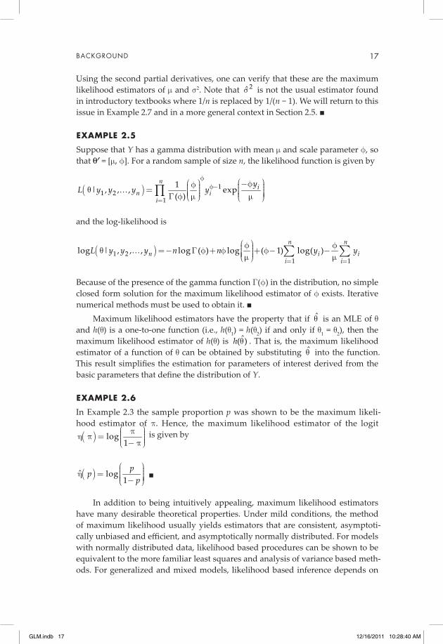
ExaMPLE 2.5

Suppose that Y has a gamma distribution with mean m and scale parameter f, so that q¢ = [m, f]. For a random sample of size n, the likelihood function is given by

( ) 11 2

1

1| , , , exp( )

ni

n ii

yL y y y y

ff-

=

æ öæ ö -ff ÷÷ çç ÷÷q ¼ = çç ÷÷ çç ÷÷ç ÷çG f m mè ø è øÕ

and the log-likelihood is

( )1 21 1

log | , , , log ( ) log ( 1) log( )n n

n i ii i

L y y y n n y y= =

æ öf f÷ç ÷q ¼ =- G f + f + f- -ç ÷ç ÷çm mè ø å å

Because of the presence of the gamma function G(f) in the distribution, no simple closed form solution for the maximum likelihood estimator of f exists. Iterative numerical methods must be used to obtain it. ■

Maximum likelihood estimators have the property that if q is an MLE of q and h(q) is a one-to-one function (i.e., h(q1) = h(q2) if and only if q1 = q2), then the maximum likelihood estimator of h(q) is ˆ( )h q . That is, the maximum likelihood estimator of a function of q can be obtained by substituting q into the function. This result simplifies the estimation for parameters of interest derived from the basic parameters that define the distribution of Y.

ExaMPLE 2.6

In Example 2.3 the sample proportion p was shown to be the maximum likeli-hood estimator of p. Hence, the maximum likelihood estimator of the logit ( ) log

1æ öp ÷ç ÷h p = ç ÷ç ÷- pè ø

is given by

( )ˆ log1

ppp

æ ö÷ç ÷h = ç ÷ç ÷÷ç -è ø ■

In addition to being intuitively appealing, maximum likelihood estimators have many desirable theoretical properties. Under mild conditions, the method of maximum likelihood usually yields estimators that are consistent, asymptoti-cally unbiased and efficient, and asymptotically normally distributed. For models with normally distributed data, likelihood based procedures can be shown to be equivalent to the more familiar least squares and analysis of variance based meth-ods. For generalized and mixed models, likelihood based inference depends on

GLM.indb 17 12/16/2011 10:28:40 AM

18 CHAPTER 2

asymptotic properties whose small sample behavior (like those typically found in much agricultural research) varies depending on the design and model being fit. As with any set of statistical procedures, there is no one-size-fits-all approach for maximum likelihood. More detailed discussions of these properties can be found in Pawitan (2001) and Casella and Berger (2002). When well-known estimation or inference issues that users should be aware of arise in examples in subsequent chapters, they will be noted and discussed in that context.

ExaMPLE 2.7

In Example 2.4, the maximum likelihood estimator of the variance of the normal distribution, s2,was shown to be

( )22

1

1ˆn

ii

y yn =

s = -å

Recall that an estimator is unbiased if its mean (or expected value) is the param-eter being estimated; that is, on average, the estimator gives the true value of the parameter. For 2s the expected value is

2 2 21 1ˆE 1nn n

æ ö æ ö-é ù ÷ ÷ç ç÷ ÷s = s = - sç çê ú ÷ ÷ç ç÷ ÷ë û è ø è ø

That is, the maximum likelihood estimator is a biased estimator of s2 with a bias of −1/n. For small sample sizes, the bias can be substantial. For example, for n = 10, the bias is 10% of the true value of s2. The negative bias indicates that the variance is underestimated, and hence, standard errors that use the estimator are too small. This leads to confidence intervals that tend to be too short, t and F statistics that tend to be too large, and, in general, results that appear to be more significant than they really are.

Note that the usual sample variance estimator taught in introductory statisti-cal methods courses, namely,

( )22 2

1

1 ˆ1 1

n

ii

nS y yn n=

æ ö÷ç ÷= - = sç ÷ç ÷- -è øå

has the expected value E[S2] = s2; it is an unbiased estimator of s2. A common ex-planation given for the use of the denominator n − 1 instead of n is that one needs to account for having to estimate the unknown mean. ■

2.5 varIatIonS on MaxIMuM LIKELIhooD EStIMatIon

The concept of accounting for estimation of the mean when estimating the vari-ance leads to a modification of maximum likelihood called residual maximum likelihood (REML). Some authors use the term restricted maximum likelihood as well. In Example 2.7, define the residuals i iZ Y Y= - . The Zi’s have mean zero and

GLM.indb 18 12/16/2011 10:28:41 AM

BACKGROUND 19

variance proportional to s2. Hence, they can be used to estimate s2 independently of the estimate of m. Applying maximum likelihood techniques to the Zi’s yields the REML estimator S2 of s2; that is, the usual sample variance is a REML estimator.

In the context of linear mixed models, residual maximum likelihood uses lin-ear combinations of the data that do not involve the fixed effects to estimate the random effect parameters. As a result, the variance component estimates associ-ated with the random effects are independent of the fixed effects while at the same time taking into account their estimates. Details concerning the implementation of residual maximum likelihood can be found in Littell et al. (2006), Schabenberger and Pearce (2002), and McCulloch et al. (2008). For linear mixed models with nor-mally distributed data, REML estimates are used almost exclusively because of the severe bias associated with maximum likelihood estimates for sample sizes typi-cal of much agricultural research. For mixed models with non-normal data, REML is technically undefined because the existence of the residual likelihood requires independent mean and residuals, a condition only satisfied under normality. However, REML-like computing algorithms are used for variance-covariance esti-mation in non-normal mixed models when linearization (e.g., pseudo-likelihood) methods are used. Section 2.7 contains additional discussion of this issue.

For certain generalized linear models, the mean–variance relationship required for adequately modeling the data does not correspond to the mean–vari-ance relationship of any member of the exponential family. Common examples include over-dispersion and repeated measures. Wedderburn (1974) developed the concept of quasi-likelihood as an extension of generalized linear model maxi-mum likelihood to situations in which a model for the mean and the variance as a function of the mean can be specified. In addition, the observations must be inde-pendent. Quasi-likelihood is defined as a function whose derivative with respect to the mean equals the difference between the observation and its mean divided by its variance. As such the quasi-likelihood function has properties similar to those of a log-likelihood function. Wedderburn showed that the quasi-likelihood and the log-likelihood were identical if and only if the distribution of Y belonged to the exponential family. In general, quasi-likelihood functions are maximized using the same techniques used for maximum likelihood estimation. Details con-cerning the implementation of quasi-likelihood can be found in McCullagh and Nelder (1989) and McCulloch et al. (2008).

2.6 LIKELIhooD BaSED aPProaCh to hYPothESIS tEStInG

Recall that we have a random sample Y1, Y2, …, Yn from a random variable Y hav-ing a probability distribution f(y | q) that depends on an unknown parameter(s) q. When testing hypotheses concerning q, the null hypothesis H0 places restrictions on the possible values of q. The most common type of alternative hypothesis H1 in linear models allows q its full range of possible values.

GLM.indb 19 12/16/2011 10:28:41 AM

20 CHAPTER 2

The likelihood function L(q | y1, y2, …, yn) can be maximized under the restric-tions in H0 as well as in general. Letting 0

ˆ( )L q and 1( )L q represent the maximum values of the likelihood under H0 and H1, respectively, the likelihood ratio

( ) ( )0 1ˆ ˆL Ll= q q

can be used as a test statistic. Intuitively, if 1( )L q is large compared to 0ˆ( )L q , then

the value of q that most likely produced the observed sample would not satisfy the restriction placed on q by H0 and, hence, would lead to rejection of H0. The test procedure based on the ratio of the maximum values of the likelihood under each hypothesis is called a likelihood ratio test.

ExaMPLE 2.8

Suppose that Y has a normal distribution with unknown mean m and unknown variance s2 so that q¢ = [m, s2]. Consider a test of the hypotheses

H0: m = m0 and s2 > 0 versus H1: m ¹ m0 and s2 > 0

where m0 is a specified value. In the more familiar version of these hypotheses, only the mean appears since neither hypothesis places any restrictions on the variance. The reader may recognize this as a one sample t test problem. Here we consider the likelihood ratio test.

Under H0, the mean is m0 so that the only parameter to be estimated is the vari-ance s2. The maximum likelihood estimator of s2 given that the mean is m0 can be shown to be

( )220 0

1

1ˆn

ii

yn =

s = - må

Under H1, from Example 2.4 the maximum likelihood estimators are

( )221

1

1ˆ ˆ and n

ii

y y yn =

m = s = -å

Substituting these estimators into the appropriate likelihoods, after some algebra the likelihood ratio reduces to

( )

( )

/220

2

n

ii

ii

y

y y

é ù- mê ú

ê úê úl= ê ú-ê úê úë û

å

å

It can be shown that

2 2 20 0 2 2

0 02 2 2 2

( ) ( ) ( )( ) ( )

1 1( ) ( ) ( ) ( 1)

i ii i

i i ii i i

y y y n yn y n y

y y y y y y n S

-m - + -m-m -m

= = + = +- - - -

å å

å å å

GLM.indb 20 12/16/2011 10:28:41 AM

BACKGROUND 21

Note that the second term in the last expression is, up to a factor of n − 1, the square of the t statistic. Hence, the likelihood ratio test is equivalent to the usual one sample t test for testing the mean of a normal distribution. ■

In Example 2.8 an exact distribution of the likelihood ratio statistic was read-ily determined. This is the case for all analysis of variance based tests for normally distributed data. When the exact distribution of the statistic is unknown or intrac-table for finite sample sizes, likelihood ratio tests are usually performed using

−2log(l) as the test statistic, where log is the natural logarithm. For generalized linear models, we use the result that the asymptotic distribution of −2log(l) is chi-squared with v degrees of freedom, where v is the difference between the number of unconstrained parameters in the null and alternative hypotheses. Practically speaking, −2log(l) having an asymptotic chi-squared distribution means that, for sufficiently large sample sizes, approximate critical values for −2log(l) can be obtained from the chi-squared table. The accuracy of the approximation and the necessary sample size are problem dependent.

For one parameter problems, ˆ ˆ( ) / var ( )¥q- q q is asymptotically normally distributed with mean zero and variance one, where q is the maximum likeli-hood estimator of q and ˆvar ( )¥ q is the asymptotic variance of q . For normally distributed data, the asymptotic variance is often referred to as the “known vari-ance.” Because the square of a standard normal random variable is a chi-square, it follows that

( )( )

2ˆ

ˆvarW

¥

q- q=

q

asymptotically has a chi-squared distribution with one degree of freedom. W is known as the Wald statistic and provides an alternative test procedure to the likelihood ratio test. More generally, for a vector of parameters q, the Wald statistic is given by

( ) ( ) ( )-

¥¢ é ù= - -ê úë û

1ˆ ˆ ˆcovW q q q q q

where ¥ˆcov ( )q

is the asymptotic covariance matrix of q . W has the same asymp-

totic chi-squared distribution as the likelihood ratio test.

ExaMPLE 2.9

Consider the one factor normal theory analysis of variance problem with K treat-ments and, for simplicity, n observations per treatment. The mean of the ith treat-ment can be expressed as mi = m + ti, subject to the restriction t1 + … + tK = 0. The parameter m is interpreted as the overall mean and the treatment effect ti as the deviation of the ith treatment mean from the overall mean. The initial hypothesis of equal treatment means is equivalent to

H0: t1 = … = tK = 0 versus H1: not all ti are zero.

GLM.indb 21 12/16/2011 10:28:41 AM

22 CHAPTER 2

The likelihood ratio statistic for testing H0 is given by/2SSE

SSE SSTrt

Knæ ö÷ç ÷l= ç ÷ç ÷+è ø

where SSTrt is the usual treatment sum of squares and SSE is the error sum of squares. We can rewrite l as

/2/2

1 1SSTrt ( 1)1 1SSE ( 1)

KnKn

K FK n

é ùæ ö÷ ê úç ÷ç ÷ ê úç ÷ç ÷ ê úl= =ç ÷÷ç ê ú-÷ç ÷ ê ú+ +ç ÷÷çè ø ê ú-ë û

where F = MSTrt/MSE has an F distribution with K − 1 and K(n − 1) degrees of freedom. Hence, the usual F-test in the analysis of variance is equivalent to the likelihood ratio test.

Because the maximum likelihood estimator of ti is the difference between the ith sample mean and the grand mean, it can be shown that the Wald statistic is given by

2SSTrtW =s

where s2 is the common variance. Replacing s2 by its estimator MSE yields a test statistic for H0; that is,

SSTrtMSE

W =

Note that W divided by the degrees of freedom associated with its numerator is the F statistic. This Wald statistic–F statistic relationship for the one factor problem will recur throughout generalized linear mixed models. ■

2.7 CoMPutatIonaL ISSuES

Parameter estimation and computation of test statistics increase in complexity as the models become more elaborate. From a computational viewpoint, linear mod-els can be divided into four groups.

• Linear models (normally distributed response with only fixed effects): For parameter estimation, closed-form solutions to the likelihood equations exist and are equivalent to least squares. Exact formulas can be written for test statistics.

• Generalized linear models (non-normally distributed response with only fixed effects): The exact form of the likelihood can be written explicitly, as can the exact form of the estimating equations (derivatives of the likelihood). Solving the estimating equations to obtain parameter

GLM.indb 22 12/16/2011 10:28:41 AM

BACKGROUND 23

estimates usually requires an iterative procedure. Likelihood ratio or Wald statistics can be computed for statistical inference.

• Linear mixed models (normally distributed response with both fixed and random effects): The exact form of the likelihood can be written explicitly as can the exact form of the estimating equations. There are two sets of estimating equations, one for estimating the model effects, commonly referred to as the mixed model equations and another for estimating the variance and covariance components. Solving the mixed model equations yields maximum likelihood estimates. These can be shown to be equivalent to generalized least squares estimates. The estimating equations for the variance and covariance are based on the residual likelihood; solving them yields REML estimates. Iteration is required to solve both sets of equations. Inferential statistics are typically approximate F or approximate t statistics. These can be motivated as Wald or likelihood ratio statistics, since they are equivalent for linear mixed models.

• Generalized linear mixed models (non-normally distributed response with both fixed and random effects): The likelihood is the product of the likelihood for the data given the random effects and the likelihood for the random effects, with the random effects then integrated out. Except for normally distributed data, the resulting marginal likelihood is intractable, and as a result, the exact form of the estimating equations cannot be written explicitly. Numerical methods such as those described below must be used. In theory, likelihood ratio statistics can be obtained. In practice, they are computationally prohibitive. Inference typically uses Wald statistics or approximate F statistics based on the Wald statistic.

Numerical techniques for finding MLEs and standard errors can be divided into two groups, linearization techniques and integral approximations. As the name implies, linearization uses a linear approximation to the log-likelihood, e.g., using a Taylor series approximation. This gives rise to a pseudo-variate that is then treated as the response variable of a linear mixed model for computational purposes. The mixed model estimating equations with suitable adjustments for the pseudo-variable and the associated estimating equations for variance and covariance components are solved. As with the linear mixed and generalized lin-ear models, the solution process is iterative. Variations of linearization include pseudo-likelihood (Wolfinger and O’Connell, 1993) and penalized quasi-like-lihood (Breslow and Clayton, 1993). The estimating equations for linear, linear mixed, and generalized linear models described above are all special cases of pseudo-likelihood.

The second group of techniques is based on integral approximations to the log-likelihood. This group includes the Laplace and Gauss–Hermite quadrature methods, Monte Carlo integration, and Markov chain Monte Carlo. The choice of a particular numerical method is problem dependent and will be discussed in the context of the various numerical examples in Chapter 5.

GLM.indb 23 12/16/2011 10:28:42 AM

24 CHAPTER 2

The most serious practical issue for iterative estimation procedures is conver-gence. Convergence is rarely a problem for generalized linear models and linear mixed models containing only variance components or at most simple covariance structures. However, as model complexity increases, the chance of encounter-ing a convergence issue increases. The science and art of resolving convergence issues is an essential part of working with generalized and mixed models. Some convergence problems can be corrected easily by using different starting values or by increasing the number of iterations allowed before failure to converge is declared. In other cases, using a different algorithm may lead to convergence. Non-convergence may also result from ill-conditioned data; that is, data with very small or very large values or data ranging over several orders of magnitude. In these cases, a change of scale may eliminate the problem. Non-convergence also can result when there are fewer observations than parameters in the model being fit. This is especially possible for models having a large number of covariance parameters. Such problems require fitting a simpler model. In generalized linear mixed models non-convergence may be due to a “flat” likelihood function near the optimum. In extreme cases, it may be necessary to relax the convergence crite-rion to obtain a solution, although this should be considered a last resort.

2.8 FIxED, ranDoM, anD MIxED MoDELS

Factors included in a statistical model of an experiment are classified as either fixed or random effects. Fixed factors or fixed effects are those in which the factor levels or treatments represent all of the levels about which inference is to be made. Fixed effects levels are deliberately chosen and are the same levels that would be used if the experiment were to be repeated. This definition applies to quantitative factors as well as qualitative effects; that is, in regression and analysis of covari-ance, the ranges of the observed values of the independent variables or covariates define the entire region to which inferences will apply. In contrast, random fac-tors or random effects are those for which the factor levels in the experiment are considered to be samples from a larger population of possible factor levels. Ideally random effects levels are randomly sampled from the population of levels, and the same levels would not necessarily be included if the experiment were to be repeated. As a consequence of these definitions, fixed effects determine a model for the mean of the response variable and random effects determine a model for the variance.

Since the levels of a random factor are a sample (ideally random) from some population of possible factor levels and that population has an associated prob-ability distribution, the random effects will also have a probability distribution. In general, it is assumed that the distribution of the random factor has a mean of zero and some unknown variance. For the mixed models discussed in this book, we further assume that random effects have normal distributions. In contrast, the factor levels of a fixed effect are a set of unknown constants.

In a given model an effect must be defined as either fixed or random. It can-not be both. However, there are certain types of effects that defy a one-size-fits-all

GLM.indb 24 12/16/2011 10:28:42 AM

BACKGROUND 25

categorization. Whether an effect is classified as fixed or random depends on how the factor levels were selected and the objectives of the experiment. For example, in a field experiment conducted at several locations, if the locations represent different crop growing regions and it is of interest to determine which of several cultivars are best suited for each region, then location would treated as a fixed effect. Inference would focus on differences among the location means. Moreover, inference is restricted to only those locations included in the experiment and cannot be extended to other locations. On the other hand, if the experiment included multiple locations to broaden the range of environmental conditions (e.g., weather, soil) under which the mean yields of the cultivars were being compared, then locations would be a ran-dom effect and inference would focus on the variability among locations. Treating locations as a random effect allows us to broaden inference to encompass the entire population of locations, not just those locations used in the experiment.

Usually fixed effects focus on the mean response and random effects focus on the variance. However, in the random location example, it may still be of interest to predict the yield of a particular cultivar at a particular location. In mixed models, this can be accomplished using best linear unbiased prediction (BLUP) that incor-porates the random effects into the estimation of the mean for a particular location.

The model for a particular experiment is called a fixed effects model if all of the factors are fixed. A random effects model is one containing only random fac-tors except for an intercept which is an unknown constant. If the model contains at least one fixed and at least one random effect, it is called a mixed model. In the early analysis of variance literature, fixed and random effects models were often referred to as model I and model II, respectively (Eisenhart, 1947).

Under the usual set of statistical assumptions for fixed effects models, the observed responses are assumed to be independent. However, this is not the case for random and mixed models. In these types of models, the random effects impose a correlation structure on the observations. For example, in a randomized complete block design with a fixed treatment factor and a random blocking effect, obser-vations taken within the same block are correlated. Hence, analysis of data from experiments based on mixed models must take the correlation structure into account.

2.9 thE DESIGn–anaLYSIS oF varIanCE–GEnEraLIzED LInEar MIxED MoDEL ConnECtIon

The analysis of variance is arguably the fundamental tool for analyzing agronomic research data. Properly understood, analysis of variance (ANOVA) can be a valu-able aid for understanding how to set up and work with generalized linear mixed models. Improperly understood, it can be a severe impediment to meaningful understanding of generalized linear mixed models and their role in agronomic research. Understanding the interconnections among ANOVA, design, and mod-eling is crucial for working effectively with generalized linear mixed models.

The analysis of variance was introduced by R.A. Fisher (Fisher and Mackenzie, 1923) in an article entitled “Studies in Crop Variation II: The Manorial Response of Different Potato Varieties.” Once analysis of variance appeared, statistical scientists

GLM.indb 25 12/16/2011 10:28:42 AM

26 CHAPTER 2

began attempts to place it in the framework of linear statistical models with vary-ing degrees of success. Unfortunately, some of their lesser efforts still plague modern statistical practice in the experimental sciences. Speed (2010) described the uneasy relationship between statistical modeling and ANOVA, citing Fisher’s remarks in the discussion accompanying Yates (1935). In those comments, Fisher (1935) described two aspects of the design of an experiment—topographical fac-tors and treatment effects. Fisher used the word “topographical” because he was referring specifically to field experiments, but the term can be understood more broadly as the design structure that gives rise to all sources of variation in the observed data other than the treatments. Modern terminology refers to Fisher’s topographical factors as the experiment design or design structure. Regardless of the terminology, the concept is important because, above all, a statistical model is a description, in mathematical and probabilistic terms, of the design and treatment factors and associated random variation giving rise to the observed data. Effective statistical modeling begins by asking “What would Fisher do?” and understand-ing his approach. Consider the following example as an illustration.

ExaMPLE 2.10

Suppose a field experiment is to be conducted to evaluate seed from two variet-ies of a certain crop using a randomized complete block design with 10 blocks. Data on several variables for each variety were taken according to the experi-ment’s protocol. A schematic diagram of the experiment is shown in Table 2–3. In practice, we would randomize the order of the varieties within each block and follow any additional requirements of the design protocol. The schematic diagram serves mainly to show the essential design and treatment structures of

the experiment.The design structure

for this experiment con-sists of the blocks and the two plots, one per variety, shown in Table 2–4. The sources of variation asso-ciated with the design structure are the varia-tion among blocks and the variation between plots within each block (Table 2–5). The treatment struc-ture is a single fixed factor consisting of the set of the two varieties. The associ-ated source of variation is the variety effect with one degree of freedom. Integrating the design and

taBLE 2–3. Diagram of the seed evaluation experiment in Example 2.10.

Block Variety

1 A B

2 A B

3 A B

4 A B

5 A B

6 A B

7 A B

8 A B

9 A B

10 A B

taBLE 2–4. Diagram of the design structure for the seed evaluation experiment in Example 2.10.

Block Plot

1 – –

2 – –

3 – –

4 – –

5 – –

6 – –

7 – –

8 – –

9 – –

10 – –

GLM.indb 26 12/16/2011 10:28:42 AM

BACKGROUND 27

treatment structures yields the ANOVA table shown in Table 2–6. Note that the one degree of freedom for varieties is taken from the degrees of freedom for plots within blocks (the experimental unit to which varieties were randomly assigned), leaving nine degrees of freedom for plots after accounting for varieties. It is important to under-stand that when Fisher conceived ANOVA, the state of the art in statistical computing was little more than pencil and paper. Given this limita-tion, the practical way to assess the statistical significance of variety effects was to compare variation attributable to varieties as measured by MS(Variety) to naturally occurring variation asso-ciated with plots within blocks as measured by MS(WithinBlocks), more commonly referred to as MS(Error) or MS(Residual).

Up to this point, the analysis can be per-formed without reference to a statistical model. Proceeding further requires a statistical model. One well-known model assumes indepen-dent, normally distributed observations on each plot. The end result is an F-test using the ratio MS(Variety)/MS(WithinBlocks). What if one or

both of these model assumptions is not true? For example, what if the response variable is binomial? Suppose in each plot we observe 100 plants of each variety and ask how many plants out of the 100 have a certain characteristic; for example, how many show evidence of damage from an insect pest or disease? This is where following Fisher’s approach of identifying the experiment’s processes becomes essential.

We begin by considering only the design structure processes.

• Design process 1: Variation among blocks. Let bi denote the effect of the ith block, i = 1, …, 10.

• Design process 2: Variation among plots within a block. Let yij denote the observation on the jth plot within the ith block, i = 1, …, 10, j = 1, 2. Note that this is an observation on the plot, not an effect, because the plot is the unit on which the data are collected.

At this point, we specify any probability assumptions. If the blocks form a sample from a larger population that just as well could have consisted of any 10 blocks from this population (i.e., if blocks effects are random), then there is a prob-ability distribution associated with the block effect. Linear mixed models and, in this book, generalized linear mixed models assume that the bi are independent and normally distributed with mean zero and variance 2

Bs .

taBLE 2–5. Sources of variation and degrees of freedom (df) for the design structure in Example 2.10.

Source of variation df

Blocks 9

Plots within blocks 10

Total 19

taBLE 2–6. ANOVA table containing sources of variation and degrees of freedom (df) for the integrated design and treatment structures in Example 2.10.

Source of variation df

Blocks 9

Varieties 1

Plots within blocks given varieties 9

Total 19

GLM.indb 27 12/16/2011 10:28:42 AM

28 CHAPTER 2

Observations on plots within blocks must be treated as random variables. Formally, in mixed model theory, each observation is conditional on the random effect level from which the observation arises. Denote this by yij | bi (the vertical bar is read as “given”). The conditional distribution has a conditional mean mij | bi and variance 2

Ws . If the conditional distribution of yij is normal, then we can express the conditional distribution of the observations as yij | bi ~ independent N(mij | bi,

2Ws ). Statistical modeling begins at this point.

Modeling consists of two steps:

• Decide on an equation that describes how the sources of variation affect mij.

• Decide whether the mechanism described by this equation affects the mean mij directly or indirectly; e.g., through the canonical parameter of the distribution.

For the normal distribution the natural or canonical parameter is the mean, and the decomposition is mij | bi = m + bi + Vj, where m represents an intercept and Vj represents the effect of the jth variety (more generally, treatment). There is a long standing tradition of calling the parameter m the overall mean. For generalized lin-ear models, this becomes a dysfunctional habit that is important to break.

Now suppose that the observations are not normally distributed. For example, how do we form a model when the observation is the number of damaged plants out of the 100 plants observed per plot? In this case the distribution of the observa-tions is yij | bi ~ independent Binomial(100, pij), where pij denotes the probability that a plant in the ith block containing the jth variety shows evidence of damage. We still want to use b0 + bi + Vj to characterize the block and variety effect on pij, where m has been replaced by b0 to reinforce the distinction between the intercept and the overall mean. There are several reasons not to use this decomposition to directly model pij, the most important being that if we do fit a model pij = b0 + bi + Vj it is pos-sible to obtain nonsensical estimates of the probability pij that are less than zero or greater than one. A better choice is to model the logit; i.e., log[pij /(1 − pij)], which is the canonical parameter for the binomial distribution (Example 2.1). The resulting model is written as hij = log[pij /(1 − pij)] = b0 + bi + Vj. In generalized linear model ter-minology, hij is called the link function and b0 + bi + Vj is called the linear predictor. ■

Two important facts emerge from Example 2.10. First, the models for both the normal and binomial distributions use the same linear predictor, in this exam-ple, b0 + bi + Vj. Relating this to Table 2–6, the predictor is the additive list of the effects in the ANOVA, excluding the last line of the table. The last line refers to the unit of observation. How that line is incorporated into the model depends on the assumed probability distribution of the observations.

Second, for the normal distribution, when we estimate the effects in the linear predictor, we have an estimate of the mean mij = b0 + bi + Vj but no information about the variance 2

Ws . We use the last line of the table to estimate this variance; i.e., 2ˆWs = MS(WithinBlocks). This is where the tradition of referring to the last line of the ANOVA table as residual or error originates. It also means that we cannot include a block × treatment interaction in the linear predictor because it is confounded

GLM.indb 28 12/16/2011 10:28:42 AM

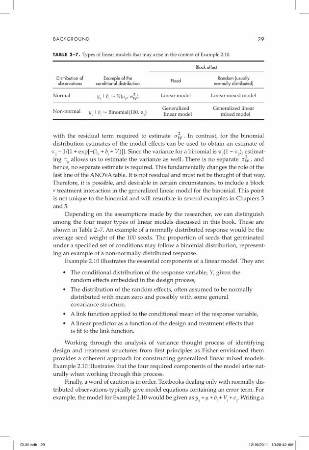
BACKGROUND 29

with the residual term required to estimate 2Ws . In contrast, for the binomial

distribution estimates of the model effects can be used to obtain an estimate of pij = 1/{1 + exp[−(b0 + bi + Vj)]}. Since the variance for a binomial is pij(1 − pij), estimat-ing pij allows us to estimate the variance as well. There is no separate 2

Ws , and hence, no separate estimate is required. This fundamentally changes the role of the last line of the ANOVA table. It is not residual and must not be thought of that way. Therefore, it is possible, and desirable in certain circumstances, to include a block × treatment interaction in the generalized linear model for the binomial. This point is not unique to the binomial and will resurface in several examples in Chapters 3 and 5.

Depending on the assumptions made by the researcher, we can distinguish among the four major types of linear models discussed in this book. These are shown in Table 2–7. An example of a normally distributed response would be the average seed weight of the 100 seeds. The proportion of seeds that germinated under a specified set of conditions may follow a binomial distribution, represent-ing an example of a non-normally distributed response.

Example 2.10 illustrates the essential components of a linear model. They are:

• The conditional distribution of the response variable, Y, given the random effects embedded in the design process,

• The distribution of the random effects, often assumed to be normally distributed with mean zero and possibly with some general covariance structure,

• A link function applied to the conditional mean of the response variable,• A linear predictor as a function of the design and treatment effects that

is fit to the link function.

Working through the analysis of variance thought process of identifying design and treatment structures from first principles as Fisher envisioned them provides a coherent approach for constructing generalized linear mixed models. Example 2.10 illustrates that the four required components of the model arise nat-urally when working through this process.

Finally, a word of caution is in order. Textbooks dealing only with normally dis-tributed observations typically give model equations containing an error term. For example, the model for Example 2.10 would be given as yij = m + bi + Vj + eij. Writing a

taBLE 2–7. Types of linear models that may arise in the context of Example 2.10.

distribution of observations

Example of the conditional distribution

Block effect

Fixed Random (usually normally distributed)

Normal yij | bi ~ N(mij , 2Ws ) Linear model Linear mixed model

Non-normal yij | bi ~ Binomial(100, pij)Generalized linear model

Generalized linear mixed model

GLM.indb 29 12/16/2011 10:28:42 AM

30 CHAPTER 2

model in this way is only valid if the conditional distribution of the observations is normal and the link function is the identity function. Otherwise, as will be seen in subsequent chapters, the equations do not make sense. On the other hand, specify-ing a model using the essential elements above is valid for any linear model.

2.10 ConDItIonaL vErSuS MarGInaL MoDELS

A distinction that arises in mixed models that does not occur in fixed effects mod-els concerns conditional and marginal modeling. Models given by the four essen-tial components listed in the previous section specify the conditional model—the name is derived from the fact that the distribution of the observations is specified conditionally on the random effects. Marginal models are an alternative way of specifying mixed models. As the name implies, they are specified in terms of the marginal distribution of the observations. The linear predictor of a marginal mod-el contains only the fixed effects. The random effects are not modeled explicitly but their impact on variation is embedded in the covariance structure of the model.

For normally distributed data (linear mixed models), the distinction is more technical than consequential. Marginal models are useful for the analysis of repeated measures and as a way of accounting for negative variance component estimates. Chapter 4 contains examples illustrating conditional and marginal lin-ear mixed models. For non-normally distributed data (generalized linear mixed models), the conditional versus marginal distinction is far more consequential because marginal models for non-normal data actually target different parameters than those we understand as we work through the model construction process described in the previous section.

Marginal models are usually called GEE-type models. The term GEE came from generalized estimating equation theory (Zeger and Liang, 1986; Liang and Zeger, 1986). Technically the term generalized linear mixed models (GLMM) refers only to conditional models. Chapter 5 begins with an illustration of the difference between conditional GLMMs and marginal GEE-type models. Other examples in Chapter 5 provide additional perspective.

2.11 SoFtWarE

Many statistical software packages can be used to analyze data from designed experiments. Only two of these, SAS (SAS Institute, Cary, NC) and R, will be de-scribed here. In our opinion, they represent the most widely used software pack-ages in the applied statistics and agricultural sciences research communities in the United States.

The impetus for the creation of SAS came from a project in the 1970s spon-sored by the Southern Region Agricultural Experiment Station directors to create a computer program to analyze data from designed experiments (Littell, 2011). Before 1990, the GLM procedure was the primary SAS tool for analyzing linear models with normally distributed responses. GLM was initially written for fixed effects models with the random statement added later to allow for random and

GLM.indb 30 12/16/2011 10:28:42 AM

BACKGROUND 31

mixed models. However, the fixed effect architecture of GLM severely limits the kinds of mixed models that can be accommodated and even with these models, its mixed model adjustments are limited. In the early 1990s, the MIXED procedure was introduced to make the full range of modeling options available for normally distributed response variables. It made the first row of Table 1–1 (normally dis-tributed data) available to researchers and provided major improvements in both the ease and accuracy of the analysis of split plot, incomplete block, repeated mea-sures, and spatial data for normally distributed responses.

The GENMOD procedure was introduced shortly after MIXED. This proce-dure made the full range of generalized linear model options available for data with fixed continuous or categorical explanatory variables as well as certain types of repeated measures and split plot analyses. However, GENMOD and MIXED together still left large portions of Table 1–1 inaccessible to researchers.

The recently introduced GLIMMIX procedure implements generalized linear mixed models. For a large range of distributions, it can address every explanatory model-response variable type combination in Table 1–1 under a common frame-work and a common syntax. This syntax is virtually identical to the syntax used by previous SAS procedures including GLM, MIXED, and GENMOD and thus is already familiar to most users.

R is a programming language for statistical computing and graphics that was designed in the early 1990s by R. Ihaka and R. Gentleman. Current developments and contributions are managed by the R Development Core Team. R is available for free as part of the GNU project. An initial installation includes a core set of packages, each containing functions to carry out specific tasks. In addition, a large number of user contributed packages on a wide variety of topics are available through the Comprehensive R Archive Network (CRAN). User contributed pack-ages can address very specific analyses of interest to the contributor. For linear mixed models and generalized linear mixed models there are both fairly gen-eral as well as more narrowly focused packages. This collection of packages only loosely overlaps what is available in SAS. In cases where a SAS procedure may not be able to fit a model, there may be a suitable package available in R.

Linear mixed models with normally distributed responses and correlated error structures can be fit using the function lme in the R package nlme. This pack-age also contains a function nlme that fits nonlinear mixed models. Several other packages are useful in special cases.

There are a number of packages in R that can fit various generalized linear models. The function glm in the package stats will fit linear models with binomial, gamma, normal, inverse normal, and Poisson responses. The function glm.nb in the package MASS allows for negative binomial distributed responses. The pack-age biglm can be used for generalized linear regression with very large data sets. The functions loglin and loglm in the package MASS fit log-linear models with binomial, multinomial, and Poisson responses.

The package MASS contains the function glmmPQL, which fits a general-ized linear mixed model with multivariate normal random effects and most of the response distributions found in SAS GLIMMIX. This function uses penalized

GLM.indb 31 12/16/2011 10:28:42 AM

32 CHAPTER 2

quasi-likelihood. The function lmer in the package lme4 will also fit generalized lin-ear mixed models using either a Laplace or Gauss–Hermite approximation to the log-likelihood and has easier to use syntax than glmmPQL. However, it does not produce F-tests and p-values. These must be calculated separately within R or else-where by the user. Alternatively, one can obtain confidence intervals on parameter estimates from their posterior distributions (created using Markov chain Monte Carlo methods) using the mcmcsamp function in the lme4 package. The model estimation method used by lmer does not allow for modeling correlation at the individual observation level. Modeling correlation at the individual observation level requires a penalized quasi-likelihood approach. The function glmm.admb in the package glmmADMB fits generalized linear mixed models for binomial, Poisson, and negative binomial distributed responses with Laplace approxima-tion as the default algorithm for likelihood estimation. The package glmmML can be used to fit binomial and Poisson responses with fixed covariates and random intercepts. The repeated package contains approximately 20 functions for fitting specialized generalized linear mixed models, many containing repeated measures.

In addition to the abovementioned packages and functions, there are a num-ber of other R packages that fit various generalized linear mixed models using other numerical techniques. There are also packages within R that take a Bayesian approach to model fitting and estimation.

In this book, we use SAS exclusively and within SAS, almost all of the exam-ples use PROC GLIMMIX. Readers are cautioned that the computational issues discussed in Section 2.7 still remain with this procedure as well as with any of the R packages. Blind acceptance of the default options of a procedure is not recom-mended and may lead to completely unreasonable results. Boykin et al. (2011) demonstrated the issues that arise when options are used that are not appropriate for the problem at hand. Examples in Chapters 4 and 5 contain specific examples of overrides of defaults essential to complete an appropriate analysis.

GLM.indb 32 12/16/2011 10:28:42 AM

BACKGROUND 33

rEFErEnCES CItEDBoykin, D., M.J. Camp, L.A. Johnson, M. Kramer, D. Meek, D. Palmquist, B. Vinyard,

and M. West. 2011. Generalized linear mixed model estimation using PROC GLIMMIX: Results from simulations when the data and model match, and when the model is misspecified. p. 137–170. In W. Song (ed.) Conference Proceedings on Applied Statistics in Agriculture. Department of Statistics, Kansas State University, Manhattan, KS.

Breslow, N.E., and D.G. Clayton. 1993. Approximate inference in generalized linear mixed models. J. Am. Stat. Assoc. 88:9–25. doi:10.2307/2290687

Casella, G., and R.L. Berger. 2002. Statistical inference. Duxbury Press, North Scituate, MA.Eisenhart, C. 1947. The assumptions underlying the analysis of variance. Biometrics

3:1–21. doi:10.2307/3001534Fisher, R.A. 1935. The design of experiments. Oliver and Boyd, Edinburgh, UK.Fisher, R.A., and W.A. Mackenzie. 1923. Studies in crop variation II: The manurial

response of different potato varieties. J. Agric. Sci. 13:311–320. doi:10.1017/S0021859600003592

Liang, K.-Y., and S.L. Zeger. 1986. Longitudinal data analysis using generalized linear models. Biometrika 73:13–22. doi:10.1093/biomet/73.1.13

Littell, R.C. 2011. The evolution of linear models in SAS®: A personal perspective. In Proceedings of SAS Global Forum 2011. Paper 325-2011. SAS Inst., Cary, NC.

Littell, R.C., G.A. Milliken, W.W. Stroup, R.D. Wolfinger, and O. Schabenberger. 2006. SAS for mixed models. 2nd ed. SAS Inst., Cary, NC.

McCullagh, P., and J.A. Nelder. 1989. Generalized linear models. 2nd ed. Chapman and Hall, New York.

McCulloch, C.E., S.R. Searle, and J.M. Neuhaus. 2008. Generalized, linear and mixed models. 2nd ed. John Wiley and Sons, New York.

Pawitan, Y. 2001. In all likelihood. Statistical modeling and inference using likelihood. Oxford Univ. Press, Oxford, UK.

Schabenberger, O., and F.J. Pearce. 2002. Contemporary statistical models for the plant and soil sciences. CRC Press, Boca Raton, FL.

Speed, T. 2010. Terence’s stuff: An ANOVA thing. IMS Bull. 39:16.Wedderburn, R.W.M. 1974. Quasi-likelihood functions, generalized linear models and

the Gauss–Newton method. Biometrika 61:439–447.Wolfinger, R., and M. O’Connell. 1993. Generalized linear mixed models:

A pseudo-likelihood approach. J. Stat. Comput. Simul. 48:233–243. doi:10.1080/00949659308811554

Yates, F. 1935. Complex experiments. Suppl. J. R. Stat. Soc. 2:181–247. doi:10.2307/2983638

Zeger, S.L., and K.-Y. Liang. 1986. Longitudinal data analysis for discrete and continuous outcomes. Biometrics 42:121–130. doi:10.2307/2531248

GLM.indb 33 12/16/2011 10:28:43 AM