analysis of fund mapping techniques for variable annuities · ii abstract our project tested the...

Worcester Polytechnic Institute

A Major Qualifying Project Report: Submitted to the Faculty of the

WORCESTER POLYTECHNIC INSTITUTE In partial fulfillment of the requirements For the Degree of Bachelor of Science by

Grant Fredricks Erin Ingalls

Angela McAlister

Date: January 15, 2010

Jon Abraham, Advisor

Guillaume Briere-Giroux, Liaison

Analysis of Fund Mapping Techniques for Variable Annuities

ii

Abstract

Our project tested the accuracy of projected mutual fund returns (via fund mappings) relative to

the actual performance of the mutual fund. To achieve this, we performed Monte-Carlo simulations

using geometric Brownian motion. Utilizing Excel’s VBA, we generated many scenarios to draw

conclusions about fund mapping reliability. We modified parameters within the simulation in order to

isolate factors that affected the fund mapping’s accuracy, and analyzed the specific effects of these

variables to provide our sponsor, Towers Perrin, with recommendations.

iii

Executive Summary

Variable annuities operate like mutual funds, except variable annuities have specific benefits

that provide the policyholder with an insurance feature. These benefits include guaranteed minimum

withdrawal benefits (GMWB), guaranteed minimum income benefits (GMIB), guaranteed minimum

accumulation benefits (GMAB), and guaranteed minimum death benefits (GMDB). The benefits provide

the policyholder with some protection against unfavorable performance of their assets, which are held

in a separate account within the variable annuity. In order to protect themselves against these

unfavorable outcomes, insurance companies use hedging programs. Hedging programs are used with

the goal of building a portfolio that is expected to increase in value in the event that the separate

account (the one providing insurance) decreases in value.

In order to build these hedging portfolios that advance in a declining market, managers use

derivative instruments that protect them against losses caused by realized volatility, interest rate

changes, and implied volatility costs. The policyholder’s separate account is invested into mutual funds

that typically use an active management strategy; however, these funds do not always have a clear

benchmark. When the benchmark is unclear, insurance companies will need to assign the mutual fund

to hedgeable indices that they will use for hedging transactions. When companies do not know the

exact benchmark, they typically regress the mutual fund returns against the historical returns of indices

that are assumed to explain the return of certain asset classes (e.g. the S&P 500 or the Russell 2000,

which we abbreviate as SPY and RUS, respectively). The process of assigning the mutual fund to

hedgeable indices is known as fund mapping. Fund mappings are used to project the expected mutual

fund performance given movement in the referenced indices.

This process inherently has a type of risk known as basis risk. Basis risk arises between an

exposure and a hedge mechanism that is not perfectly correlated with the exposure, where the degree

of the risk is based on the correlation between the exposure and the hedge (Banks, 2004). This means

that there is always a risk from inaccurate fund mappings or active management. For an insurance

company, it is impossible to directly trade derivatives with the separate account mutual funds as the

underlying asset. Consequently, insurance companies use hedgeable indices to define proxy hedge

instruments (Briere-Giroux, 2009). When the proxy hedge instrument does not use the correct

hedgeable indices, it could result in losses because of basis risk. The reason for this could be due to an

incorrect estimation of the fund mappings. Another possible source of basis risk could be that the

insurance company found the correct fund mappings given the historical performance, but the fund

managers change their strategies from one period to the next. The final source of basis risk is that the

iv

insurance company found the correct fund mapping to use going forward as a benchmark, but the

manager is trying to beat the benchmark. Therefore, there is some deviation between the benchmark

and the performance the manager is expecting, which would give rise to basis risk.

Our project studied the last source of basis risk. To do this, we tested the accuracy of projected

mutual fund returns (using fund mappings) relative to the actual performance of a mutual fund (called

MFI). MFI was created by us to follow the returns of SPY with some additional random error, which

represents the manager alpha. Manager alpha is the amount of randomness of the MFI, the risk

resulting from a manager trying to outperform the benchmark. To achieve this, we performed Monte-

Carlo simulations using geometric Brownian motion. With Excel’s Visual Basic for Applications (VBA), we

were able to generate and analyze a large number of stock simulations and regressions in order to help

us draw conclusions about the fund mapping reliability, and how manager alpha affects the accuracy of

the fund mappings. Furthermore, we modified certain parameters within the simulation, such as

manager alpha, in order to isolate specific factors that may have affected the fund mapping’s accuracy.

By analyzing the results, we were able to make conclusions about the outcomes of our research.

We discovered that basis risk arising from active management is insignificant using our model. In

general, the returns of the proxy MFI using the fund mappings were very close to the true MFI returns.

Additionally, the two-index fund mapping was almost exactly the same as the fund mapping using just

the SPY, showing that adding other indices to a fund mapping does not adversely affect the outcome,

even if those indices are not accurate. However, fund mappings based entirely on inappropriate indices

generated some error. We also found that regressing over a larger period of time created regression

coefficients that were closer to the proper fund mappings. However, this did not have a significant

impact on the actual accuracy of the fund mappings when looking ten years into the future. That means

that we found no difference between the accuracy of the fund mappings using a 1-year regression and a

10-year regression, even though the coefficients for longer regressions were more accurate.

After observing a single case and its results, we created more cases with different parameters in

order to see how they affected the outcome. Throughout 15 different cases, we changed variables such

as the manager alpha of the MFI, proportion of randomness from SPY returns for the MFI, correlation

between the SPY and RUS, and volatility of the SPY and RUS. There are several factors that we looked at

to determine the differences among the different cases, including the regressions’ coefficients of

determination (R2), realized manager alpha, realized correlation, and the ending difference between MFI

and the fund mappings. First of all, we found that increasing and decreasing the correlation and

volatility had the largest impact on the fund mapping accuracy, especially when using improper indices.

v

As the difference between the SPY and RUS volatilities increased, the accuracy of the RUS-only fund

mapping decreased. Multicollinearity did not occur, even thought the SPY and RUS are highly

correlated. This may be because using the SPY as a fund mapping was too perfect for the MFI. All other

findings were ordinary and expected; for example, there is slightly more error in the fund mappings

when the MFI has a higher manager alpha. Our results allowed us to provide our sponsor, Towers

Perrin, with recommendations on how to account for basis risk and its effects.

Although we did not find surprising results in general, future research may provide greater

insight into basis risk and the effects of active management. If our model were improved to be more

applicable to the real world, more surprising or interesting results may be found. Some ways to improve

the model may be to implement stochastic parameters, add more indices and have a more diversified

portfolio, or change the expected returns for the indices. For example, it is questionable to assume that

indices correlated in the past will continue to be correlated in the future, so future research could create

scenarios wherein the correlation or volatility changes over time. It may also be interesting to attempt

to study other sources of basis risk. For example, to study the effects of managers changing investment

strategies from one period to the next, researchers may have to do a more qualitative study on human

nature and how it affects management and investment styles. We hope that by continuing research on

the effects and sources of basis risk, insurance companies and asset managers will eventually be able to

improve their investment strategy and performance, and reduce the risk associated with variable

annuities and mutual funds.

vi

Table of Contents

Abstract .................................................................................................................................................. ii

Executive Summary ................................................................................................................................ iii

Table of Figures .................................................................................................................................... viii

Table of Tables ....................................................................................................................................... ix

1. Introduction ........................................................................................................................................ 1

2. Background ......................................................................................................................................... 2

2.1. Variable Annuities ......................................................................................................................... 2

2.2. Mutual Funds ................................................................................................................................ 4

2.3. Hedging Techniques and Hedge Funds .......................................................................................... 9

2.4. Active Management .................................................................................................................... 13

2.5. Tracking Error or Active Risk ....................................................................................................... 14

2.6. Basis Risk .................................................................................................................................... 16

2.7.1. Black-Scholes Model for Estimating Volatility ....................................................................... 18

2.7.2. Geometric Brownian Motion ................................................................................................ 18

2.7.3. Stock Correlation and Cholesky Decomposition .................................................................... 19

2.7.4. Generating Correlated Brownian Motions ............................................................................ 20

2.8. Regression Analysis ..................................................................................................................... 21

3. Methodology ..................................................................................................................................... 23

3.1. Outline of the Simulation Process ............................................................................................... 23

3.1.1. Past Data .............................................................................................................................. 25

3.1.2. The Future-Past .................................................................................................................... 25

3.1.3. Regressions .......................................................................................................................... 25

3.1.4. The Future-Future ................................................................................................................ 26

3.2. Creating the Simulation .............................................................................................................. 27

3.2.1. Inputs ................................................................................................................................... 27

3.2.1.1. The Future-Past ............................................................................................................. 27

3.2.1.2. SPY and RUS .................................................................................................................. 28

3.2.1.3. Mutual Fund .................................................................................................................. 28

3.2.1.4. Regressions ................................................................................................................... 29

3.2.1.5. The Future-Future ......................................................................................................... 29

vii

3.2.2. Scenario Output ................................................................................................................... 30

3.2.3. Output ................................................................................................................................. 31

3.2.4. Graph Data ........................................................................................................................... 32

3.2.5. Graphs ................................................................................................................................. 32

4. Analysis and Discussion ..................................................................................................................... 35

4.1. Regression Coefficients ............................................................................................................... 35

4.2. Values of R2................................................................................................................................. 36

4.3. Realized Alpha and Correlation ................................................................................................... 38

4.4. Ending Difference between MFI and MFI2Var ............................................................................. 40

4.5. Ending Difference between MFI and MFISPY ............................................................................... 41

4.6. Ending Difference between MFI and MFIRUS .............................................................................. 41

5. Conclusions and Recommendations ................................................................................................... 44

5.1. Conclusions ................................................................................................................................. 44

5.1.1. Correlation ........................................................................................................................... 44

5.1.2. Multicollinearity ................................................................................................................... 44

5.1.3. Volatility............................................................................................................................... 45

5.1.4. Regression Periods ............................................................................................................... 45

5.1.5. How Our Results Relate to Active Management and Basis Risk ............................................. 46

5.2. Improvements and Future Research ........................................................................................... 47

5.2.1. Creating Stochastic Parameters ............................................................................................ 47

5.2.2. More Scenarios .................................................................................................................... 48

5.2.3. Adding more indices ............................................................................................................. 48

5.2.4. Choice of Means for SPY and RUS ......................................................................................... 49

5.3. Final Conclusions ........................................................................................................................ 49

Bibliography .......................................................................................................................................... 50

Appendix A: Sponsor Information .......................................................................................................... 53

Appendix B: Acronyms ........................................................................................................................... 54

Appendix C: Definitions ......................................................................................................................... 55

Appendix D: VBA Code .......................................................................................................................... 57

viii

Table of Figures

Figure 1: Change in Composition of Ownership within Four Main Investment Options ............................. 5

Figure 2: U.S. Households owning Mutual Funds ..................................................................................... 6

Figure 3: Diagram .................................................................................................................................. 24

Figure 4: Example of the first type of chart generated by the Macro ...................................................... 34

Figure 5: Example of the second type of chart generated by the Macro ................................................. 34

ix

Table of Tables

Table 1: How Households Invest their IRA’s During 2008 ......................................................................... 7

Table 2: Traditional Mutual Funds versus Hedge Funds.......................................................................... 10

Table 3: Management Strategies and Characteristics ............................................................................. 11

Table 4: 2-Variable Regression Data Output........................................................................................... 30

Table 5: 1-Variable Regression Data Output........................................................................................... 31

Table 6: Defining Cases .......................................................................................................................... 35

Table 7: Regression Coefficients ............................................................................................................ 36

Table 8: Average Values of R2 ................................................................................................................ 37

Table 9: Realized Alpha and Correlation................................................................................................. 39

Table 10: Difference between MFI and MFI2Var .................................................................................... 40

Table 11: Difference between MFI and MFISPY ...................................................................................... 41

Table 12: Difference between MFI and MFIRUS ..................................................................................... 42

Table 13: Effect of volatility on improper fund mappings ....................................................................... 45

1. Introduction

Variable annuities operate like mutual funds; however, variable annuities have specific benefits

that provide the policyholder with an insurance feature. These benefits include guaranteed minimum

withdrawal benefits (GMWB), guaranteed minimum income benefits (GMIB), guaranteed minimum

accumulation benefits (GMAB), and guaranteed minimum death benefits (GMDB). The benefits provide

the policyholder with some protection against unfavorable performance of their assets, which are held

in a separate account within the variable annuity. In order to protect themselves against these

unfavorable outcomes, insurance companies use hedging programs. Hedging programs are used with

the goal of building a portfolio that is expected to increase in value in the event that the separate

account (the one providing insurance) decreases in value. Shorting the market is one possible option for

hedging this risk.

In order to build these hedging portfolios that advance in a declining market, managers use

derivative instruments which protect them against losses caused by realized volatility, interest rate

changes, and implied volatility costs. The policyholder’s separate account is invested in mutual funds

that typically use an active management strategy; however, these funds do not always have a clear

benchmark. When the benchmark is unclear, insurance companies will need to assign the mutual fund

to hedgeable indices that they will use for their hedging transactions. When companies do not know the

exact benchmark, they typically regress the mutual fund returns against the historical returns of indices

that are assumed to explain the return of certain asset classes (e.g. the S&P 500 or the Russell 2000).

The process of assigning the mutual fund to hedgeable indices is known as fund mapping. Fund

mappings are used to project the expected mutual fund performance given the movement in the

reference indices.

Our project tested the accuracy of the projected mutual fund returns (using fund mappings)

relative to the actual performance of a mutual fund (called MFI). MFI was created to follow the returns

of the S&P 500 with some random error, which represents the manager alpha. To achieve this, we

performed Monte-Carlo simulations using geometric Brownian motion. With Excel’s Visual Basic for

Applications (VBA), we were able to generate and analyze a large number of scenarios to help us draw

conclusions about the fund mapping reliability. Furthermore, we modified certain parameters within

the simulation, such as volatility and correlation, in order to isolate specific factors that may have

affected the fund mapping’s accuracy. This allowed us to analyze the specific effects of these variables

and provide our sponsor, Towers Perrin, with recommendations.

2

2. Background

In this background section, we present information about various subjects in order to help the

reader fully understand the process and goal of our project. We will begin with a very broad description

of what a variable annuity consists of and a general description of how mutual funds work. We will then

move on to discuss what hedging is and techniques used in hedge funds, which is followed by a

description on active management and basis risk. Lastly, we introduce various mathematical tools and

equations used to provide us with a hedging technique that can be analyzed and discussed.

2.1. Variable Annuities

Variable annuities are the most rapidly growing financial product today; nominal sales more

than doubled in the United States between 1996 and 2004 (Poterba, 2006). By definition, an annuity is

a contract issued by an insurance company which usually has two phases, the accumulation phase and

the payout phase (Wyss, 2001). An individual purchases a variable annuity contract by making a single

purchase payment or a series of such payments over a set period of time (Variable Annuites: What you

should know, 2009).

During the accumulation phase the annuity operates much like a mutual fund where one can

choose a variety of investment options, which consist of stocks, bonds, money market instruments, or a

combination of the three. Over time, the value of the annuity will increase or decrease depending on

the investment combination and how well the chosen funds are performing in the market (Variable

Annuites: What you should know, 2009). Furthermore, the contract value is developed using fixed or

variable investments that are tax deferrable as long as the earnings stay within the annuity (Wyss,

2001). The fixed investment is an option given by the issuer, where the insured can allocate a portion of

his or her purchase payment into a fixed account, which accumulates using a fixed interest rate (Variable

Annuites: What you should know, 2009). This fixed account is typically known as a guaranteed minimum

accumulation benefit (GMAB). More benefit options for variable annuities will be discussed later. The

insured is typically allowed to transfer funds from one investment to another without tax charges, but

other charges may be set depending on the limitations arranged by the insurer. However, if the insured

withdraws money from the account, particularly in the early stages of the accumulation phase, the

insurer will issue a surrender charge. Additionally, if withdrawals are made before the policyholder is 59

½ years of age there will be a 10% federal tax penalty (Variable Annuites: What you should know, 2009).

When the insured is prepared to enter the payout phase, there are a number of options

available. The three most common payout plans are as follows:

3

• Lump-sum: The recipient can choose to withdraw all the funds in a lump-sum payment, where

taxes are charged on the total accumulated earnings. This will result in a large tax liability,

making this option less desirable.

• Systematic Payments: This option allows a fixed amount to be paid out to the recipient at

specific time intervals until it exhausts all accumulated earnings. This option spreads out the tax

liability but must be monitored to make sure payments do not end prior to death of the

recipient.

• Annuitization: This option makes a steady stream of payments, where the insurance company

agrees to provide the recipient with an income for a specified period. Changes to these plans

are limited and tax liabilities are spread out. A portion of each payment is treated as a return of

principal (Wyss, 2001).

There are many different annuitization options: guaranteed income until the death of the

recipient, at which time payments are stopped; guaranteed payments for a specified amount of time

and in case of the recipient death, the beneficiary receives payments until funds are exhausted; and

lifetime payments to two designated people wherein if one dies the other will receive payments until his

or her death (Wyss, 2001). The variable annuity also has a guaranteed minimum income benefit (GMIB)

option, which guarantees a minimum level of the annuity income payments even if the account doesn’t

hold enough money at the time of the payment (possibly due to investment losses) (Variable Annuites:

What you should know, 2009). In order to protect against decreasing account earnings, there is a

guaranteed minimum withdrawal benefit (GMWB) option. This benefit enables the policyholder to be

able to withdraw a percentage of the initial investment every year until the entire investment has been

withdrawn (Investopedia, 2009).

The payout period differentiates the two types of accounts, fixed and variable. When dealing

with the fixed account, the policyholder will receive fixed dollar payments depending on earnings

accrued during the accumulation phase. However, when dealing with the variable account, the income

payments depend on the market value of the portfolio created during the accumulation phase. As the

value of the portfolio rises or declines, the amount of the variable income payment could increase or

decrease. During rising markets, this may be an opportunity for the income to keep pace with inflation

during the retirement years (Wyss, 2001).

There are many reasons why individuals are attracted to variable annuities, one being the desire

to accumulate wealth while not being taxed on the earnings until the policyholder makes withdrawals.

4

Another appealing reason is the insurance component of the variable annuity. The guaranteed

minimum death benefit (GMDB) option states that if the policyholder dies before they retire, their

beneficiary will receive either all the earnings accumulated thus far or some guaranteed minimum,

whichever is greater (Variable Annuites: What you should know, 2009). There is also a ‘step up’ option

that locks in any increase in market value of the variable account for the beneficiaries. Moreover, the

benefit is paid directly to the beneficiary without any costs or time delays (Wyss, 2001).

An additional reason why variable annuities may be attractive is because of the convenience

factor. Variable annuities offer a rebalancing option that restores the policyholder’s assets to their

initial state and original target allocations (Wyss, 2001). Furthermore, there is also an option of turning

the account into a life annuity at the end of the accumulation phase (mentioned previously as

annuitization), but does not force withdrawal when the policyholder reaches 70 ½ years of age (Poterba,

2006). Some insurance companies have also offered features such as ‘bonus credits’. When making a

purchasing payment, the contract promises to add a bonus credit to your account determined by a

specified percentage (usually between 1% and 5%) of the purchasing payment. However, when the

contract offers bonus credits it usually means there is an offsetting downside to the annuity, such as a

higher surrender charge, a longer surrender period and/or a higher annual mortality or risk charge

(Variable Annuites: What you should know, 2009).

The variable account accumulates earnings, as stated previously, by investing in stocks, bonds

and/or money market instruments. When creating this account, the insurance company and the client

develop a contract that acts as a mutual fund. They are able to decide which combination of

investments to choose, which are generally more risky than those investments found in the fixed

account. Furthermore, after the client chooses the contract which best suits their preferences, the

insurance company sees their contract and hedges against the risk that may arise due to the chosen

funds and benefit options. We will discuss the hedging procedure and risk in subsequent sections;

however, mutual funds represent a large portion of the variable account and are extremely important

for successful accounts.

2.2. Mutual Funds

A mutual fund is a diversified portfolio funded by various investors, with assets such as stocks,

bonds, short-term money market instruments or other securities (Mutual Funds, 2007). The investors

purchase shares of the mutual fund, which are redeemable, meaning that they can sell the shares back

to the fund at any time. When purchasing and selling funds, investors use four main sources:

5

professional financial advisers, employer sponsored retirement plans, fund companies, and fund

supermarkets. When individuals are just beginning to invest, most depend on financial advisers to make

intelligent decisions for them in order to earn a good return on their investments. In 1990, financial

advisers were responsible for 72% of households who had assets in mutual funds (Investment Company

Fact Book, 2009). Many investors study the performances of mutual funds in the past, study the

progress of the funds, and may turn to a stockbroker for an informed decision (Wolfinger, 2005).

Generally, funds focus on specific characteristics of stocks, such as buying stocks for dividends or long-

term growth, while others focus on industries or the geographic location (Wolfinger, 2005). Other

investment options will be discussed in further detail later.

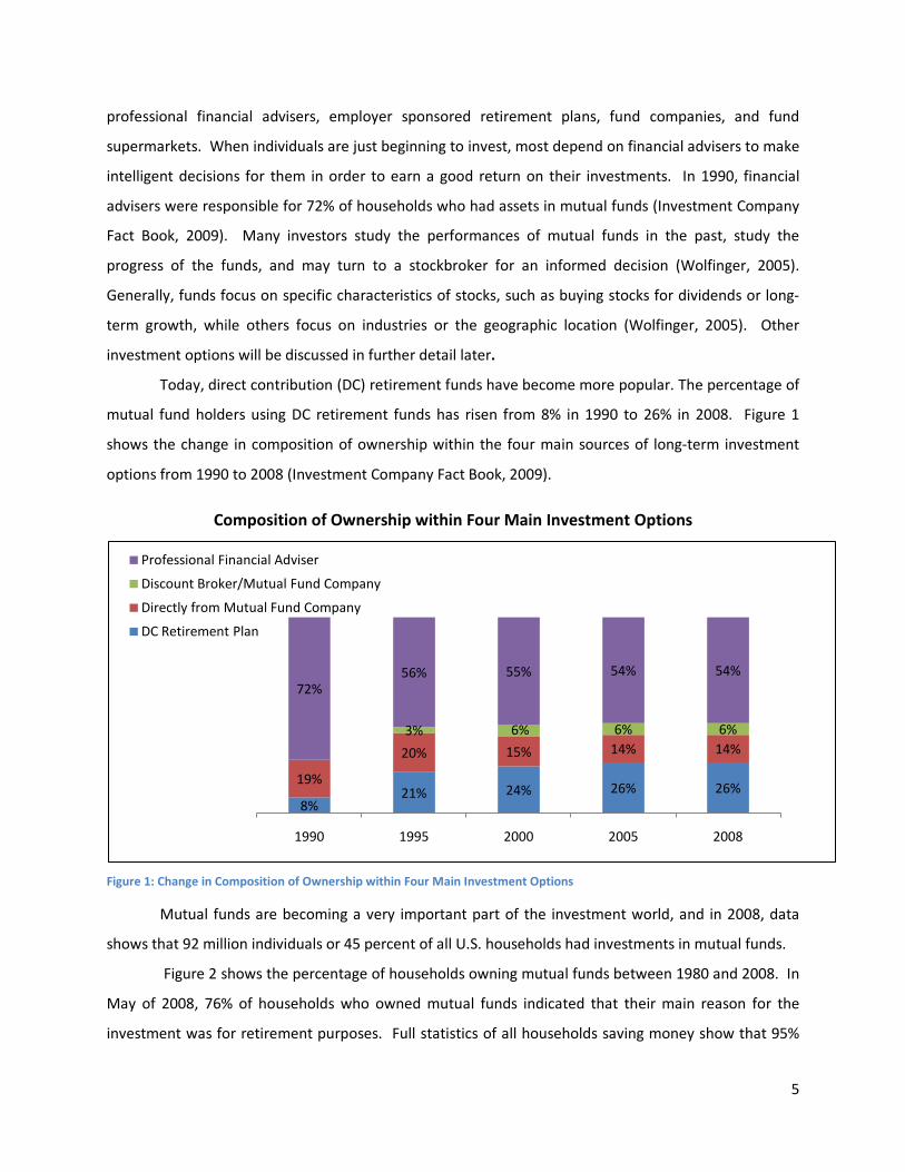
Today, direct contribution (DC) retirement funds have become more popular. The percentage of

mutual fund holders using DC retirement funds has risen from 8% in 1990 to 26% in 2008. Figure 1

shows the change in composition of ownership within the four main sources of long-term investment

options from 1990 to 2008 (Investment Company Fact Book, 2009).

Composition of Ownership within Four Main Investment Options

Figure 1: Change in Composition of Ownership within Four Main Investment Options

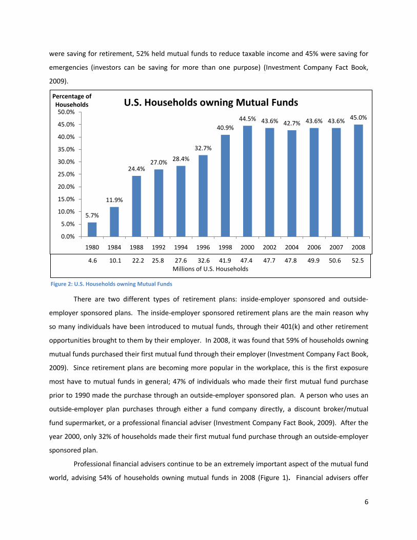
Mutual funds are becoming a very important part of the investment world, and in 2008, data

shows that 92 million individuals or 45 percent of all U.S. households had investments in mutual funds.

Figure 2 shows the percentage of households owning mutual funds between 1980 and 2008. In

May of 2008, 76% of households who owned mutual funds indicated that their main reason for the

investment was for retirement purposes. Full statistics of all households saving money show that 95%

8%21% 24% 26% 26%

19%

20% 15% 14% 14%3% 6% 6% 6%

72%56% 55% 54% 54%

1990 1995 2000 2005 2008

Professional Financial Adviser

Discount Broker/Mutual Fund Company

Directly from Mutual Fund Company

DC Retirement Plan

6

were saving for retirement, 52% held mutual funds to reduce taxable income and 45% were saving for

emergencies (investors can be saving for more than one purpose) (Investment Company Fact Book,

2009).

There are two different types of retirement plans: inside-employer sponsored and outside-

employer sponsored plans. The inside-employer sponsored retirement plans are the main reason why

so many individuals have been introduced to mutual funds, through their 401(k) and other retirement

opportunities brought to them by their employer. In 2008, it was found that 59% of households owning

mutual funds purchased their first mutual fund through their employer (Investment Company Fact Book,

2009). Since retirement plans are becoming more popular in the workplace, this is the first exposure

most have to mutual funds in general; 47% of individuals who made their first mutual fund purchase

prior to 1990 made the purchase through an outside-employer sponsored plan. A person who uses an

outside-employer plan purchases through either a fund company directly, a discount broker/mutual

fund supermarket, or a professional financial adviser (Investment Company Fact Book, 2009). After the

year 2000, only 32% of households made their first mutual fund purchase through an outside-employer

sponsored plan.

Professional financial advisers continue to be an extremely important aspect of the mutual fund

world, advising 54% of households owning mutual funds in 2008 (Figure 1). Financial advisers offer

4.6 10.1 22.2 25.8 27.6 32.6 41.9 47.4 47.7 47.8 49.9 50.6 52.5 Millions of U.S. Households

5.7%

11.9%

24.4%27.0% 28.4%

32.7%

40.9%44.5% 43.6% 42.7% 43.6% 43.6% 45.0%

0.0%

5.0%

10.0%

15.0%

20.0%

25.0%

30.0%

35.0%

40.0%

45.0%

50.0%

1980 1984 1988 1992 1994 1996 1998 2000 2002 2004 2006 2007 2008

Percentage of Households U.S. Households owning Mutual Funds

Figure 2: U.S. Households owning Mutual Funds

7

investment services and planning services. Investment services include regular portfolio reviews and

recommendations, and recommendations for the employee sponsored retirement plans. Planning

services include discussing financial goals, planning to achieve specific goals (such as college and

retirement), and managing assets in retirement. The recipients also have access to specialists regarding

areas such as tax planning (Investment Company Fact Book, 2009).

There are various ways for individuals to invest; however, mutual funds hold the majority of

investments. Table 1 shows the diversity in individual retirement account (IRA) holdings. Variable

annuities are the fourth largest investment option available, providing 23% of households with

individual retirement accounts. Individual bonds and U.S. saving bonds hold a much lower percentage

than previous years because the purchasing of these bonds have declined dramatically since 2005

(Treasury Direct, 2008).

How Households Invest their IRA’s During 2008 (percentage, multiple responses included)

Mutual Funds (total) 73

Stock MFs 61

Bond MFs 37

Hybrid MFs 22

Money Market MFs 33

Individual Stocks 42

Annuities (total) 34

Variable Annuity 23

Fixed Annuity 21

Bank Savings Accounts 28

Individual Bonds 13

U.S. Savings Bonds 10

ETFs 8

Other 7

Table 1: How Households Invest their IRA’s During 2008

Source: (Investment Company Fact Book, 2009)

8

There are various types of mutual funds that are offered to investors, including:

Corporate Bonds: Bonds issued by corporations, which pay higher rates due to their riskiness (Corporate

Bonds, 2009).

Growth Funds: Growth of capital is the main objective of this type of fund, which is composed mostly of

common stocks. These funds can be either conservative (investing in large cap) or aggressive (investing

in small cap).

Sector Funds: Invest in companies in a specific geographic area or industry.

Income Funds: Provide investors with a high yield by investing in stocks and bonds that make dividend

payments to shareholders.

Balanced Funds: Have a conservative investment policy invested in common stock, preferred stock and

bonds.

US Government Securities Funds: Invest in securities offered by the U.S. government, such as Treasury

bills, notes, and bonds.

Money Market Funds: These investors have a high return and high liquidity, which are high-yield short-

term debt securities.

International Funds: Invest in common stocks of foreign countries.

(Finance, 2005)

Mutual funds have many benefits and conveniences. When investing in a mutual fund,

investment decisions are made by full-time investment managers, where they can invest in full or

fractional shares. These shares can be used as collateral for a loan, which is very beneficial to the

shareholders. The shareholders are also offered a conversion privilege, which allows the investor to

change from one fund to another (within the same family) if the investor thinks it will provide capital

gains (Finance, 2005).

When investing in mutual funds, the shares are always open to the public and continuously

redeemable shares are sold by the investor. The investor buys shares at the ask price and sells the

9

shares at the bid price, where the ask price cannot be larger than the bid price by 8.5% under National

Association of Securities Dealers law (Finance, 2005).

After the client has chosen their mutual fund contract, the next step is to send the contract to

the insurance company. When the insurance company receives this contract, they try to hedge against

the funds based on the riskiness of the investments they chose. Insurance companies use many hedging

techniques in order to provide them with confidence about the risk that may arise. Furthermore, there

are also hedge funds that are used by many investors. Insurance companies hedging for variable

annuities do not use hedge funds due to their risky nature; however, typical techniques for hedging can

be seen in hedge funds.

2.3. Hedging Techniques and Hedge Funds

When working with any investment there are always risks and rewards involved. Generally, the

lower the risk of an investment, the lower the potential reward. Managers are constantly trying to

develop a trade-off between the two. Anytime an investor is defraying risk by investing in an offsetting

investment, they are hedging their risk (Chriss, 1996). For example, a manager with a call option is

always exposed to the risk that their stock price would rise above their strike price (price in which the

security can be bought, at expiration) (Strike Price, 2009). At expiration of the stock, the manager will

need to have cash equal to the difference between the market price of the stock and the strike price,

assuming the market price is exceeds the strike price. In order to hedge against this risk, the manager

would invest in a separate security which, at expiration, would provide the cash difference needed for

the previous investment (Chriss, 1996). This is one example of a hedging technique.

Black-Scholes is a method used for hedging techniques, and if the weights on each investment

are kept in balance, then the value of the portfolio and the option are always equal (Chriss, 1996).

When hedging techniques are used for variable annuities, the manager uses this method in order to

provide the necessary benefits the insured had chosen (described above: GMAB, GMDB, GBIB, GMWB).

An example of hedging techniques can be seen in hedge funds.

As mentioned above, variable annuities are usually split between two accounts. The variable

account is invested into mutual funds that are actively managed. In order to minimize risk, the manager

needs to create an account that will increase as the market decreases, also known as shorting the

market. Hedge funds work the same way as traditional mutual funds do, where various investors pool

together funds in order to create a diversified portfolio. However, a hedge fund manager’s main

concern is reducing the risk within the portfolio. Due to this, the managers are much more flexible

10

when choosing their investments and are given investment tools and techniques that managers of

traditional mutual funds do not implement (Wolfinger, 2005).

Since the 1990’s, hedge funds have soared in popularity. There are an estimated 6000 hedge

funds active today managing $600 billion in assets, whereas only 68 hedge funds were active in 1984

(Lhabitant, 2004). There are many different definitions of a hedge fund, but the most important

characteristic is that they are not open to the public. François-Serge Lhabitant, the author of Hedge

Funds: Quantitative Insights, has provided a starting definition: “Hedge funds are privately organized,

loosely regulated and professionally managed pools of capital not widely available to the public.” Due

to the private nature of a hedge fund, regulators do not feel it is a traditional investment vehicle (like

mutual funds) and therefore there is no reason to regulate it or require specific disclosers (Lhabitant,

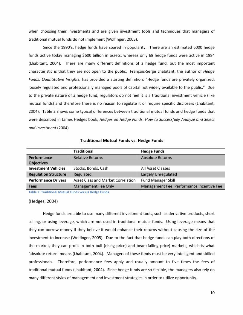
2004). Table 2 shows some typical differences between traditional mutual funds and hedge funds that

were described in James Hedges book, Hedges on Hedge Funds: How to Successfully Analyze and Select

and Investment (2004).

Traditional Mutual Funds vs. Hedge Funds

Traditional Hedge Funds

Performance Objectives

Relative Returns Absolute Returns

Investment Vehicles Stocks, Bonds, Cash All Asset Classes Regulation Structure Regulated Largely Unregulated Performance Drivers Asset Class and Market Correlation Fund Manager Skill Fees Management Fee Only Management Fee, Performance Incentive Fee Table 2: Traditional Mutual Funds versus Hedge Funds

(Hedges, 2004)

Hedge funds are able to use many different investment tools, such as derivative products, short

selling, or using leverage, which are not used in traditional mutual funds. Using leverage means that

they can borrow money if they believe it would enhance their returns without causing the size of the

investment to increase (Wolfinger, 2005). Due to the fact that hedge funds can play both directions of

the market, they can profit in both bull (rising price) and bear (falling price) markets, which is what

‘absolute return’ means (Lhabitant, 2004). Managers of these funds must be very intelligent and skilled

professionals. Therefore, performance fees apply and usually amount to five times the fees of

traditional mutual funds (Lhabitant, 2004). Since hedge funds are so flexible, the managers also rely on

many different styles of management and investment strategies in order to utilize opportunity.

11

Management Strategies and Characteristics

Category Sub strategy Risk Volatility Focus

Global Macro (tactical)

Global Macro Managed futures Emerging Mkts

High Very High

Opportunistic Exploitation of Macro trends

One way speculation on future movements

Event Driven

Merger Arbitrage Distressed Securities

Special Situations

Medium Low

Exploit unrealized value Transaction and time driven

Equity Hedges Long/Short

Short Selling Medium to

high Medium to

high

Combine L/S equity and bonds to reduce market exposure and

isolate performance while managing risk

Relative Value/Mkt

Neutral

Convertible Fixed Income

Equity Mkt Neutral Low Low

Exploit pricing inefficiencies Neutralize L/S positions

Minimize directional effect

Funds of Funds Strategy Specific Sector Specific

Low Low to

moderate Stock diversification

Long-term stabilization Table 3: Management Strategies and Characteristics

(Hedges, 2004)

Global Macro, or tactical trading investment style, focuses on the direction of the market prices

representing currencies, commodities, equities and/or bonds (Lhabitant, 2004). Global Macros are the

purest form of top-down investing techniques and base their actions on changes within fundamental

economic, political and market factors (Lhabitant, 2004). Global Macro managers’ portfolios are very

large, but very concentrated on specific investment themes. These managers rely heavily on derivatives

and leverage, along with goals of high returns and more liberal attitudes towards risk then other styles

of investing (Hedges, 2004). Commodity trading advisers and managed futures managers are included in

this category, and are usually split into two groups: systematic traders and discretionary traders.

Systematic traders believe that the future movements of the market can be explained by historical data

and spend much of their time using computer-generated systems to reduce volatility. Discretionary

traders proceed with decisions based on fundamentals and technical market analysis, along with their

past experiences and trading skills (Lhabitant, 2004).

The event-driven style focuses on price fluctuations and imbalances during a specific life cycle of

a company, such as during mergers and acquisitions, bankruptcy, corporate reconstruction or spin-offs

12

(Lhabitant, 2004). This style can be broken down into four sub strategies: distressed securities, risk

(merger) arbitrage, special situations and sector funds (Hedges, 2004). Distressed security funds focus

on the debt or equity of companies that are expected to be in financial or operational distress, which are

long-term with long redemption periods (Lhabitant, 2004). The managers of these funds are often

referred to as vulture investors and become actively involved with the reconstruction of the company

(Hedges, 2004). Risk arbitrage funds focus on companies that are involved in a merger or acquisition,

where they buy stocks of the acquired company. This tends to be a riskier investment because if the

take-over is broken the investor could lose a large amount; therefore, the managers prefer not to get

involved with companies who have hostile takeovers (Hedges, 2004). Special situations fall under

multiple themes, including distressed securities and risk arbitrage. The managers focus on underlying

problems within the companies, such as emerging market debt, depressed stocks, unannounced

mergers/acquisitions or reorganization that would drop the stock prices temporarily (Hedges, 2004).

Lastly, sector funds focus on specific sectors of the economy, such as technology companies, financial

institutions, healthcare and biotech companies, etc. (Hedges, 2004).

Equity hedges, much like the name indicates, are when managers invest in equity and make long

investments with short sales in order to reduce, but not eliminate, market exposure (Lhabitant, 2004).

These funds tend to have more long gross exposure than short gross exposure, which implies that the

funds have a significant correlation with traditional mutual funds and experience large downturns when

the market experiences large downturns (Lhabitant, 2004). Equity hedges can also be classified into

several sub strategic categories: global, regional, sectoral, emerging and dedicated short bias, which

proves them to be very opportunistic (Lhabitant, 2004).

Relative value/market neutral funds seek to effectively neutralize market influences, where their

profit will come from the difference in price between two securities (Hedges, 2004). The strategies used

by these funds include convertible arbitrage, fixed-income arbitrage, index arbitrage, closed-end fund

arbitrage, and equity market neutral (Hedges, 2004). Convertible arbitrage exploits pricing

abnormalities between bonds that are convertible and their equity (Lhabitant, 2004). The fixed-income

arbitrage exploits pricing inefficiencies within and across global fixed income markets. These funds are

known to be very profitable, but unpredictable (Hedges, 2004). Index arbitrage exploits the mispricing

of indices and index derivative securities (Lhabitant, 2004). However, since computerized trading has

increased in popularity, the mispricing of indices has decreased and therefore this method does not

provide much profit (Hedges, 2004). Closed-end fund arbitrage buys a basket of stocks or securities and

replicates a closed-end mutual fund. The key interest for these managers is to find mutual funds that

13

are selling securities at substantially different prices from their net asset value (Hedges, 2004). Lastly,

equity market neutral strategies exploit pricing inefficiencies between related equity and equity

derivative securities using tools designed to completely eliminate nearly all market risk (Hedges, 2004).

Funds of Funds are defined as a breed of mutual funds where managers invest in traditional

mutual funds and hedge funds (Wolfinger, 2005). This method gives the ability to use all strategies that

each manager prefers instead of only using a single strategy. The investments in hedge funds will

reduce the potential for poor performance and the diversification of the portfolio will yield long-term

returns (Lhabitant, 2004).

Today, equity hedging funds are the dominant strategy and are a direct result of the bear

market in the early 2000s. Long-only managers were forced to drop their traditional mutual funds and

open hedge funds in order to short sell short and obtain performance fees (Lhabitant, 2004).

In order for insurance companies to gain profits for clients, and also for their own benefit, they

must be very active in their management styles. One component of active management is the manager

alpha, which represents the risk that is uncorrelated with the market, with a goal of decreasing the

deviation between the fund mapping and the indices used (Litterman, 2005).

2.4. Active Management

There are two main strategies for managing a portfolio, active management and passive

management. Active management involves constantly buying and selling a specific mix of securities in

hopes of out-performing the market (Curtis, 2001). Passive management is the opposite of active

management, wherein the manager of the mutual fund tries to mirror already existing market indices

(Lim, 2005). Jack Bogle, founder of the Vanguard Group, describes the difference between active and

passive management as follows: “Active fund managers seek to find those needles in the haystack that

lead to outsized results; passively managed index funds simply buy the whole haystack” (Lim, 2005).

According to the tracking service of Morningstar, of 16,000 mutual funds in existence an estimated 95%

of them are actively managed (Lim, 2005).

One type of active management is qualitative management. A qualitative manager will choose

stocks based on an analysis of their income statements and balance sheets, financial ratios, phone

interviews with company personnel, research reports, and the manager’s intuition and experience

(Chincarini & Kim, 2006). Another strategy is quantitative management (also known as QEPM,

quantitative equity portfolio management), which is not based on intuition like qualitative management.

These managers base decisions on mathematical and statistical analyses. Quantitative managers look at

14

the stock fundamentals from the income statement and balance sheet, technical data, macroeconomic

data, survey data, analyst’s recommendations or any other data stored in a database (Chincarini & Kim,

2006). With the technological advancements of the last decade, quantitative management is growing in

popularity, since computers can process information faster and the internet offers more information

which is available at all times. However, even with all of the information available, qualitative

management is also growing in popularity.

In Grinold and Kahn’s Active Portfolio Management (2000), they developed a fundamental law

of active management. The variables in the formula consist of the following:

Breadth Coefficient (BC): The number of independent forecasts taken per year.

Information Coefficient (IC): The measure of skill correlating each forecast and the actual outcome.

Information Ratio (IR): Measure of the manager’s opportunity.

With these variables, the measure of the manager’s opportunity (IR) can be computed as:

IR = IC⋅√𝑩𝑩𝑩𝑩

This formula can be used for giving insight into active management, but is not an investment

tool (Grinold & Kahn, 2000). In short, this law indicates that low-turnover strategies (lower BC) have to

be very accurate (higher IC) in order to produce the same information ratio (IR) as high-turnover

strategies (Fundamental Law of Active Management, 2007).

There are a few ways an insurance company could improve their risk-adjusted returns, such as

by separating their interest rate, market, and active risk. Furthermore, an insurance company could

manage their market risk more effectively and decrease the exposure their liabilities may have to

interest rate fluctuations. Some also believe that taking more active risk could be beneficial to their risk-

adjusted returns (Active Alpha and Beyond, 2009).

2.5. Tracking Error or Active Risk

Tracking error or active risk represents how well a portfolio tracks the fund mapping. When

using hedging procedures, managers use Monte-Carlo simulation to develop many possible scenarios in

order to test how their mutual fund may react to specific market changes. The simulated mutual fund

represents how they believe the market will move and is known as a fund mapping. The fund mapping

is used as a tool to analyze how well their mutual fund is performing. The size of the tracking risk

15

depends generally on the size of the active portfolio, not on the scope of the fund mapping (Hull, 2006).

In order for the manager to minimize the tracking error, they need to study the stocks’ expected

returns, volatilities, and the correlation between the stocks (Chincarini & Kim, 2006). After taking all of

these factors into consideration, the manager will decide the correct weights of each stock in order to

minimize the error and maximize the return. The determined weights are very important in minimizing

the tracking error and there are many methods for determining the best weights.

The first method is known as the Ad Hoc method, which is when the manager chooses a

specified number of stocks with the largest market capitalization as the fund mapping (Chincarini & Kim,

2006). However, there are some downfalls to this method. The first problem is that this fund mapping

would be very sensitive depending on its size. The second problem is that there is no attempt to choose

a fund mapping that minimizes tracking error, because the manager only chooses the stocks based on

their market capitalization. Lastly, the fund mapping has to be very large in order to represent the

market correctly. For example, if the manager chooses the 50 stocks that have the largest market

capitalization, it only represents 50% of the S&P 500, and represents a smaller percentage of certain

larger indices (Chincarini & Kim, 2006). Although simple, this method is not the best method in

determining the fund mapping.

Another method in determining the fund mapping is stratification. This was originally used by

statisticians in order to gather characteristics about a certain population when they could not afford to

gather information on all the members. Therefore, this method uses a representative sample of the

population (Chincarini & Kim, 2006). The strategy is to select portions of each type of stock in order to

represent the universe of stocks. The risk is minimized by the diversification of the portfolio; however, it

does not give the manager confidence to judge what kind or how much risk they are dealing with

(Chincarini & Kim, 2006).

The best method that managers use is the minimization-of-tracking-error approach. There are

two methods used in this approach. One method is to minimize the tracking error, while the other is to

maximize the expected excess returns without going over the maximum tracking error determined by

the manager (Chincarini & Kim, 2006). Most managers define the tracking error as the standard

deviation of the difference between the portfolio’s returns and the fund mapping’s returns. The

following equation is used to minimize the tracking error:

𝑇𝑇𝑇𝑇 = 𝑆𝑆𝑆𝑆(𝑟𝑟𝑃𝑃 − 𝑟𝑟𝐵𝐵) = �𝑉𝑉𝑉𝑉𝑟𝑟(𝑟𝑟𝑃𝑃 − 𝑟𝑟𝐵𝐵)

16

where 𝑟𝑟𝑃𝑃 = portfolio return, 𝑟𝑟𝐵𝐵 = fund mapping return, 𝑆𝑆𝑆𝑆 represents standard deviation, 𝑉𝑉𝑉𝑉𝑟𝑟

represents variance (Chincarini & Kim, 2006).

The manager’s goal is to get the tracking error to equal zero; however, in reality this is very

difficult due to transaction costs, reinvestment of dividends and methods of sampling the fund mapping

(Chincarini & Kim, 2006). What is most important is keeping the tracking error stable. Furthermore, the

tracking error is usually annualized; the manager can use the same equation given above except to

annualize it they would need to multiply the result by the square root of the number of periods per year

they are analyzing. For example, if a person were dealing with months he or she could multiply the

result by √12 to annualize it (Chincarini & Kim, 2006).

When tracking how well the portfolio is doing relative to the chosen fund mapping, there is

always a risk that arises between the hedging instruments and the movement of the liability. This is

known as basis risk. This is the topic of the next section.

2.6. Basis Risk

When an insurance company performs hedging for liabilities, there will be a mismatch between

the performance of the hedging instruments and the movement in the liability. A large contributor for

that difference is called basis risk. Basis risk is a risk that arises between an exposure and a hedge

mechanism that is not perfectly correlated with the exposure, where the degree of the risk is based on

the correlation between the exposure and the hedge (Banks, 2004). Basis risk typically takes place when

an imperfect hedging product is used as a proxy hedge for the exposure because the correct hedge is

expensive or very hard to find (Horcher, 2005). For an insurance company, it is impossible to directly

trade derivatives with the separate account mutual funds as the underlying. As a consequence

insurance companies use hedgeable indices to define proxy hedge instruments (Briere-Giroux, 2009).

When the proxy hedge instrument does not use the correct hedgeable indices, it could result in

losses because of basis risk. The reason for this could be due to an incorrect estimation of the fund

mappings. Another possible source of basis risk could be that the insurance company found the correct

fund mappings given the historical performance, but the fund managers change their strategies from

one period to the next. The final source of basis risk is that the insurance company found the correct

fund mapping to use going forward as a benchmark, but the manager is trying to beat the benchmark.

Therefore, there is some deviation between the benchmark and the performance the manager is

expecting, which would give rise to basis risk.

17

In the end, the risk is present when the predicted fund performance does not match the actual

fund performance. This means that the change in value of the hedge instruments does not properly

offset the change in the value of the liabilities. The following equation could give some insight into the

interpretation of basis risk:

Basis = Spot price of asset to be hedged - Futures price of contract used

The spot price is the price that the manager expects the asset to be, and the future price is the

market determined price of the asset at a certain date in the future. The basis is zero when the spot

price of assets to be hedged and the future price of contract used are equal. The basis increases when

the spot price increases more that the futures contract, which is referred to as a strengthening of the

basis. The weakening of the basis happens when the future price is more than the spot price (Hull,

2006).

When basis risk is being measured, there is a hedging tool already set in place, as mentioned

above. The hedging procedures are used to reduce this risk as well, by using mathematical tools in

order to predict how the hedging tool may react to specific conditions. To predict this, we created a

model for equity returns that attempted to simulate various market conditions.

2.7. Model for Equity Returns

Our model for equity returns can be thought of as a Monte-Carlo method. The Monte-Carlo

method consists of observing a large number of possible random outcomes in order to predict what the

true result or outcome will be. We employed Monte-Carlo methods in our model for equity returns by

creating many scenarios (or ‘worlds’) of how markets may move in the future. Specifically, our Monte-

Carlo simulation occurs in an artificial environment in order to generate the random process of market

prices and rates (Crouhy, Galai, & Mark, 2001). Each simulation is a scenario that represents a possible

‘world’ which produces future stock prices and is used for risk management (Dash, 2004). When

generating many scenarios, the distribution of the stock prices is expected to converge towards the true

distribution (Crouhy, Galai, & Mark, 2001).

The Monte-Carlo simulation using Brownian motion involves two main steps. The first step

involves finding the risk factors and estimating parameters such as volatility and correlation using the

historical data of the stock prices and returns (Crouhy, Galai, & Mark, 2001). The second step is to use

geometric Brownian motion to construct price paths, which are created using a normal random number

generator.

18

2.7.1. Black-Scholes Model for Estimating Volatility

In order to model a single stock or index, a manager must know some historical information

about the stock or index. Specifically, he or she must be able to estimate the drift rate and volatility.

The drift rate is the expected return of a stock in a given time period. If a stock price increases 6% per

year on average, then the drift rate is 6%. Volatility is a measure of uncertainty about the returns of a

stock or index (Hull, 2006). Volatility is more difficult than drift rate to estimate, since it depends on the

amount of variance over all times, as opposed to just the beginning and end of a period of time.

Given a series of stock prices from 𝑆𝑆0 to 𝑆𝑆𝑛𝑛 , the Black-Scholes method for estimating volatility

from historical data is

𝜎𝜎 = � 1𝑛𝑛 − 1∑ ((𝑢𝑢𝑖𝑖 − ū)2)𝑛𝑛

𝑖𝑖=1

√𝜏𝜏=𝑆𝑆𝑆𝑆(𝑢𝑢𝑖𝑖)√𝜏𝜏

where 𝑢𝑢𝑖𝑖 = ln � 𝑆𝑆𝑖𝑖𝑆𝑆𝑖𝑖−1

�, ū = ∑ 𝑢𝑢𝑖𝑖𝑛𝑛𝑖𝑖=1𝑛𝑛

, 𝑛𝑛 + 1 = number of observations, and 𝜏𝜏 = length of time between 𝑆𝑆𝑖𝑖

and 𝑆𝑆𝑖𝑖+1 in years (Hull, 2006). In words, the estimate of the volatility is the standard deviation of all log

returns divided by the square root of the amount of time between each observation (in years). Once

the annual volatility and drift rate are estimated, one can begin to simulate the stock price in the future.

2.7.2. Geometric Brownian Motion

Geometric Brownian motion is a method used to simulate stock prices over time. This model is

known to be a very powerful and flexible one, but it can only be used for portfolios of a limited size due

to the amount of computer resources it requires (Crouhy, Galai, & Mark, 2001). Given a drift rate

(expected return) µ, annual volatility 𝜎𝜎, initial stock price 𝑆𝑆𝑡𝑡 , and a standard normal random number 𝜀𝜀

�𝜀𝜀~𝑁𝑁(0,1)�, the stock price at time 𝑡𝑡 + 𝛥𝛥𝑡𝑡 is given by the equation

𝑆𝑆𝑡𝑡+Δ𝑡𝑡 = 𝑆𝑆𝑡𝑡 exp��𝜇𝜇 − 𝜎𝜎2

2�Δ𝑡𝑡 + 𝜎𝜎𝜀𝜀√Δ𝑡𝑡�.

This is the same as saying that 𝑆𝑆𝑡𝑡+𝛥𝛥𝑡𝑡 is lognormal, or that

ln(𝑆𝑆𝑡𝑡+𝛥𝛥𝑡𝑡) ~𝑁𝑁�ln(𝑆𝑆𝑡𝑡) + �𝜇𝜇 −𝜎𝜎2

2 � 𝑡𝑡,𝜎𝜎2𝑡𝑡�

(Hull, 2006).

This process can be used over and over in order to simulate a stock price at various times,

beginning at 𝑆𝑆𝑡𝑡 and continuing for each 𝛥𝛥𝑡𝑡 interval. At each time, the previous value of 𝑆𝑆𝑡𝑡+Δ𝑡𝑡 becomes

the new 𝑆𝑆𝑡𝑡 , a new 𝜀𝜀 is found, and a new 𝑆𝑆𝑡𝑡+Δ𝑡𝑡 is calculated.

19

2.7.3. Stock Correlation and Cholesky Decomposition

Generating a simulation for one index is straightforward, because during the simulation there is

no other factor which it may affect or be affected by. However, when generating two or more

correlated indices, the effect that one index has on the others must be considered. Although each index

moves randomly during each iteration of geometric Brownian motion depending upon the value of 𝜀𝜀, if

the indices are correlated, the values of 𝜀𝜀 used for each index should be correlated.

The first step in determining how to correlate indices using geometric Brownian motion is to

estimate their correlation in the past. Although it may be questionable to assume that indices

correlated in the past will continue to be correlated in the future, estimating correlation in the past can

still guide the modeling of correlation in the future. Given two indices, 𝑋𝑋1 and 𝑋𝑋2, the correlation

between the indices is given by

𝐶𝐶𝐶𝐶𝑟𝑟𝑟𝑟(𝑋𝑋1,𝑋𝑋2) = 𝜌𝜌 =𝐶𝐶𝐶𝐶𝐶𝐶 (𝑋𝑋1,𝑋𝑋2)

�𝑉𝑉𝑉𝑉𝑟𝑟(𝑋𝑋1) ∗ 𝑉𝑉𝑉𝑉𝑟𝑟(𝑋𝑋2)

where 𝐶𝐶𝐶𝐶𝐶𝐶(𝑋𝑋1,𝑋𝑋2) = 𝑇𝑇��[𝑋𝑋1𝑋𝑋2]�� − 𝑇𝑇[𝑋𝑋1] ∗ 𝑇𝑇[�𝑋𝑋2�] and 𝑉𝑉𝑉𝑉𝑟𝑟(𝑋𝑋𝑛𝑛) = 𝑇𝑇��[(𝑋𝑋𝑛𝑛)2]�� − (�𝑇𝑇[𝑋𝑋𝑛𝑛 ]�)2.

Once the correlation is found, it can be used to model correlated random numbers. In our case,

we want to create a correlation matrix that will be used in the geometric Brownian motion formula to

generate correlated indices. The size of the correlation matrix depends upon the number of correlated

indices being modeled; if there are 𝑛𝑛 indices, then the correlation matrix will be 𝑛𝑛𝑥𝑥𝑛𝑛. For the two-index

case, the correlation matrix 𝐶𝐶 is easy to create:

𝐶𝐶 = �𝜎𝜎1 0𝜎𝜎2𝜌𝜌 𝜎𝜎2�1− 𝜌𝜌2�

where 𝜎𝜎1 and 𝜎𝜎2 are the estimated volatilities of the indices, and 𝜌𝜌 is the desired correlation between

the two (Haugh, 2004). This matrix 𝐶𝐶 can be written as two horizontal vectors:

𝐶𝐶 = �𝑽𝑽1𝑽𝑽2�

Where 𝑽𝑽1 = (𝜎𝜎1, 0) and 𝑽𝑽2 = �𝜎𝜎2𝜌𝜌, 𝜎𝜎2�1− 𝜌𝜌2�. When modeling two indices, this is all that is

needed.

However, when three or more correlated indices are to be generated, finding the correlation

matrix is more difficult. Given n indices 𝑋𝑋1 ··· 𝑋𝑋𝑛𝑛 , we must first create a covariance matrix ∑:

∑ = �

𝐶𝐶𝐶𝐶𝐶𝐶(𝑋𝑋1,𝑋𝑋1) 𝐶𝐶𝐶𝐶𝐶𝐶 (𝑋𝑋1,𝑋𝑋2)𝐶𝐶𝐶𝐶𝐶𝐶 (𝑋𝑋2,𝑋𝑋1) 𝐶𝐶𝐶𝐶𝐶𝐶(𝑋𝑋2,𝑋𝑋2) ⋯ 𝐶𝐶𝐶𝐶𝐶𝐶 (𝑋𝑋1,𝑋𝑋𝑛𝑛)

𝐶𝐶𝐶𝐶𝐶𝐶 (𝑋𝑋2,𝑋𝑋𝑛𝑛)⋮ ⋱ ⋮

𝐶𝐶𝐶𝐶𝐶𝐶 (𝑋𝑋𝑛𝑛 ,𝑋𝑋1) 𝐶𝐶𝐶𝐶𝐶𝐶 (𝑋𝑋𝑛𝑛 ,𝑋𝑋2) ⋯ 𝐶𝐶𝐶𝐶𝐶𝐶(𝑋𝑋𝑛𝑛 ,𝑋𝑋𝑛𝑛)

�.

20

Note that 𝐶𝐶𝐶𝐶𝐶𝐶(𝑋𝑋𝑖𝑖 ,𝑋𝑋𝑖𝑖) = 𝑉𝑉𝑉𝑉𝑟𝑟(𝑋𝑋𝑖𝑖) and that 𝐶𝐶𝐶𝐶𝐶𝐶�𝑋𝑋𝑖𝑖 ,𝑋𝑋𝑗𝑗 � = 𝐶𝐶𝐶𝐶𝐶𝐶�𝑋𝑋𝑗𝑗 ,𝑋𝑋𝑖𝑖�. To find the correlation matrix 𝐶𝐶

based on this covariance matrix ∑, we must find the Cholesky Decomposition of ∑ (Haugh, 2004).

The Cholesky Decomposition of a matrix ∑ is defined as 𝐶𝐶 such that ∑ = 𝐶𝐶𝑇𝑇𝐶𝐶. In other words,

the correlation matrix 𝐶𝐶 multiplied by its transpose 𝐶𝐶𝑇𝑇 should equal the covariance matrix ∑. The

process of finding 𝐶𝐶 such that ∑ = 𝐶𝐶𝑇𝑇𝐶𝐶 is very difficult for large matricies, and often requires the use

of a computational program, such as MATLAB or VBA (Haugh, 2004). In general, the form of 𝐶𝐶 will be

𝐶𝐶 =

⎣⎢⎢⎢⎡𝑉𝑉1,1 0 0𝑉𝑉2,1 𝑉𝑉2,2 0𝑉𝑉3,1 𝑉𝑉3,2 𝑉𝑉3,3

⋯000

⋮ ⋱ ⋮𝑉𝑉𝑛𝑛 ,1 𝑉𝑉𝑛𝑛 ,2 𝑉𝑉𝑛𝑛 ,3 ⋯ 𝑉𝑉𝑛𝑛 ,𝑛𝑛⎦

⎥⎥⎥⎤

where each 𝑉𝑉𝑖𝑖,𝑗𝑗 is a positive real number. Like the 2x2 case, 𝐶𝐶 can be written as a series of horizontal

vectors:

𝐶𝐶 = �

𝑽𝑽1𝑽𝑽2⋮𝑽𝑽𝑛𝑛

�

with each 𝑽𝑽𝑖𝑖 representing a row in 𝐶𝐶. Note that the 2x2 form of 𝐶𝐶 can also be found using this method

of Cholesky decomposition, but it is much easier to just use the general form of the 2x2 correlation

matrix.

2.7.4. Generating Correlated Brownian Motions

Once the correlation matrix is found, geometric Brownian motion can be used to generate

correlated random indices. The process is similar to the process above, except that instead of having

one standard normal random number ε �𝜀𝜀~𝑁𝑁(0,1)�, there must be 𝑛𝑛 independent standard normal

random numbers 𝜀𝜀1 ··· 𝜀𝜀𝑛𝑛 , where 𝑛𝑛 is the number of correlated indices. Each 𝜀𝜀𝑖𝑖 must be generated

independently from all of the others. Once all 𝜀𝜀𝑖𝑖 are generated, put them in a vector

𝒁𝒁 = �

𝜀𝜀1𝜀𝜀2⋮𝜀𝜀𝑛𝑛

�.

Finally, once the random vector is created, use it in the formula for geometric Brownian motion

to find the next value of each index. The price of index 𝑖𝑖 at time 𝑡𝑡 is denoted 𝑆𝑆𝑖𝑖,𝑡𝑡 , and the price of each

index at time 𝑡𝑡 + ∆𝑡𝑡 is

𝑆𝑆1,𝑡𝑡+Δ𝑡𝑡 = 𝑆𝑆1,𝑡𝑡 exp��𝜇𝜇1 −𝜎𝜎1

2

2 �Δ𝑡𝑡 + 𝑽𝑽1 ∙ 𝒁𝒁√Δ𝑡𝑡�

21


2

2 �Δ𝑡𝑡 + 𝑽𝑽2 ∙ 𝒁𝒁√Δ𝑡𝑡�

⋮

𝑆𝑆𝑛𝑛 ,𝑡𝑡+Δ𝑡𝑡 = 𝑆𝑆𝑛𝑛 ,𝑡𝑡 exp��𝜇𝜇𝑛𝑛 −𝜎𝜎𝑛𝑛2

2 �Δ𝑡𝑡 + 𝑽𝑽𝑛𝑛 ∙ 𝒁𝒁√Δ𝑡𝑡�

where 𝜇𝜇1 ∙∙∙ 𝜇𝜇𝑛𝑛 are the drift rates (expected returns) of each index, 𝜎𝜎1 ∙∙∙ 𝜎𝜎𝑛𝑛 are the estimated

volatilities of each index, 𝑽𝑽1 ∙∙∙ 𝑽𝑽𝑛𝑛 are the rows of the correlation matrix, and 𝒁𝒁 is the vector composed

of independent standard normal random variables. Note that 𝑽𝑽𝑖𝑖 ∙ 𝒁𝒁 is the dot product of 𝑽𝑽𝑖𝑖 and 𝒁𝒁

(Haugh, 2004). Once one iteration of geometric Brownian motion is complete, it can be repeated over

and over with a new standard normal random variable vector 𝒁𝒁.

The two-index case that is used throughout our simulations is a bit simpler than the general case

above for 𝑛𝑛 correlated indices. When geometric Brownian motion is used to generate two correlated

indices, the price at time 𝑡𝑡 + ∆𝑡𝑡 is


2

2 �Δ𝑡𝑡 + 𝜎𝜎1𝜀𝜀1√Δ𝑡𝑡�


2

2 �Δ𝑡𝑡 + �𝜎𝜎2𝜌𝜌𝜀𝜀1 + 𝜎𝜎2𝜀𝜀2�1 − 𝜌𝜌2�√Δ𝑡𝑡�

where 𝜇𝜇1 and 𝜇𝜇2 are the drift rates (expected returns) of each index, 𝜎𝜎1and 𝜎𝜎2 are the estimated

volatilites of each index, 𝜌𝜌 is the correlation between the two indices, and 𝜀𝜀1 and 𝜀𝜀2 are two

independent standard normal random numbers. Note that these formulas are the same as the ones

above, except that 𝑽𝑽1 and 𝑽𝑽2 have been replaced with their exact values from the 2x2 correlation

matrix, and 𝒁𝒁 replaced with 𝜀𝜀1 and 𝜀𝜀2. This model can be repeated as many times as desired, creating a

random walk of correlated indices into the future. Using geometric Brownian motion to generate a

large number of random scenarios of stock prices is a type of Monte-Carlo simulation.

2.8. Regression Analysis

While conducting the Monte-Carlo Simulation, it was previously explained that historical data

were used to provide the managers with parameters in order to execute the Brownian motion. After

the Monte-Carlo simulation is complete, the mutual fund being used as a benchmark is regressed

against the market indices chosen in order to see which market index best explains the movement of

the mutual fund. The regression analysis is extremely important in determining the relationship

between two or more variables. Linear regressions find the relationship between a dependent variable

22

and an independent variable, whereas multiple regressions have a dependent variable and two or more

independent variables (Multiple Regression, 2008). When finding the relationship between the

variables, it does not necessarily mean that one variable causes the other, but there is some significant

involvement between the variables (Linear Regression, 1997-1998). In other words, regressions can

determine correlation but not causation.

The numerical measurement of the relation between the two variables is known as the

correlation coefficient (or the slope of the regression line), denoted as beta (β) (Linear Regression, 1997-

1998). When β equals one, it shows that the variables are perfectly correlated and will move along the

same path. When β is negative it means that the variables move in opposite directions (Levinson, 2005).

When saying that the variables move in opposite directions, it means that when one variable increases,

the other is expected to decrease. Furthermore, when β equals zero, it means that there is no

relationship between the two variables. In most cases involving stock regressions, the independent

variable represents the market and the dependent variable represents the stock to be benchmarked.

When the β coefficient is 1.5, this shows that the stock is expected to rise or fall 1.5% when the market

rises or falls 1% (Levinson, 2005). A high positive β means that the share is riskier and when beta is

positive but less than one it represents a conservative investment (Levinson, 2005).

For a linear regression, the equation will only involve two variables:

𝑌𝑌 = 𝛼𝛼 + 𝛽𝛽 ∗ 𝑋𝑋

where Y represents the dependent variable, α is the intercept, β is the correlation coefficient and X is

the independent variable (Linear Regression, 1997-1998). When we have a multiple regression, the

equation will be:

𝑌𝑌 = 𝛼𝛼 + 𝛽𝛽1 ∗ 𝑋𝑋1 + 𝛽𝛽2 ∗ 𝑋𝑋2 + ∙∙∙ +𝛽𝛽𝑛𝑛 ∗ 𝑋𝑋𝑛𝑛 .

In this equation, the X’s represent the different independent variables with the corresponding

correlation coefficients (Multiple Regression, 2008).

23

3. Methodology

This chapter discusses the procedures we used in order to achieve our goals and objectives. The

first section provides a brief outline of the steps we performed, including subsections discussing each

step in further detail. The subsections explain how we used historical data to develop parameters

needed to carry out a Monte-Carlo Simulation and how we applied regression analysis to analyze

benchmark accuracy. The second section discusses the spreadsheet we constructed using Excel’s Visual

Basic for Applications (VBA).

3.1. Outline of the Simulation Process

First, we performed ten-year simulations of the RUS (iShares Russell 2000 Index) and SPY (S&P

depository receipts or SPDR) using geometric Brownian motion based on their historical data. In

addition, for each simulation of the SPY we created MFI (our simulated mutual fund, called Mutual

Funds Incorporated), which had the same expected daily returns as the SPY, except with a small random

error every day that represented the manager alpha. Next, we performed regressions comparing the

returns of the MFI with the returns of the SPY and RUS, which gave us fund mappings for the MFI.

Following this, we performed additional ten-year simulations of the SPY, RUS, and MFI that began where

each of the initial simulations ended. We also computed what the value of the MFI would have been

given the fund mapping determined in the regression. By comparing the differences between how the

MFI actually performed and how its fund mappings performed, we were able to determine the accuracy

of regression analysis for creating fund mappings. For a diagram explaining our simulations, see Figure 3.

This process can be summarized in four steps:

1) Analyzing actual historical data for the SPY and RUS.

2) Simulating the initial ten years (the ‘Future-Past’).

3) Regressing the MFI returns against the SPY and RUS returns.

4) Simulating ten more years, beginning where the first simulations ended, as well as

computing the value of the MFI based on the fund mappings. This final is simulation is

done many times, to get a large distribution of outcomes (the ‘Future-Future’).

.

.

.

.

.

.

.

.

.

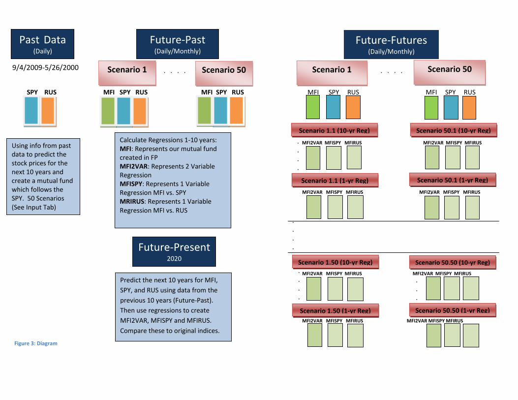
9/4/2009-5/26/2000

.

.

.

.

.

.

.

.

.

.

.

.

.

. . . .

. . . .

SPY RUS MFI SPY RUS MFI SPY RUS MFI SPY RUS MFI SPY RUS

MFI2VAR MFISPY MFIRUS MFI2VAR MFISPY MFIRUS




Past Data (Daily)

Future-Past (Daily/Monthly)

Scenario 50

Future-Futures (Daily/Monthly)

Calculate Regressions 1-10 years: MFI: Represents our mutual fund created in FP MFI2VAR: Represents 2 Variable Regression MFISPY: Represents 1 Variable Regression MFI vs. SPY MRIRUS: Represents 1 Variable Regression MFI vs. RUS

Scenario 1.1 (10-yr Reg) Scenario 50.1 (10-yr Reg)

Predict the next 10 years for MFI, SPY, and RUS using data from the previous 10 years (Future-Past). Then use regressions to create MFI2VAR, MFISPY and MFIRUS. Compare these to original indices.

Using info from past data to predict the stock prices for the next 10 years and create a mutual fund which follows the SPY. 50 Scenarios (See Input Tab)

Scenario 1.1 (1-yr Reg)



Scenario 50

Scenario 1



Future-Present 2020

Scenario 1


Figure 3: Diagram

After completing this process for one scenario, we can continue to repeat steps 2-4 in order to

generate a large distribution of possible outcomes. For our purposes, we performed 50 simulations of

the Future-Past, with 50 Future-Future simulations for each Future-Past.

3.1.1. Past Data

We began our research by analyzing historical data of the SPY and RUS. We obtained daily

values of the SPY and RUS dating back to May 26, 2000 from Yahoo Finance (SPY - S&P Dep Receipts,

2009). Both the SPY and RUS indexes represent total returns (including dividends). Using the Black-

Scholes method for estimating volatility, we estimated the volatility of the SPY and RUS from May 26,

2000 to September 4, 2009. In addition to estimating the volatility of the SPY and RUS, we determined

the correlation between their daily returns. Based on the SPY and RUS’s volatility and correlation, we

were able to create a covariance matrix and find the Cholesky decomposition of this matrix. The

Cholesky decomposed matrix was used during the simulation to model the correlation between the SPY

and RUS, based on their past correlation and volatility.

3.1.2. The Future-Past

The first part of our simulation was called the Future-Past (FP). First, we simulated the SPY and

RUS using geometric Brownian motion for ten years. Then, we generated a MFI that followed the SPY

simulation with some amount of random error to represent manager alpha. In other words, we created

a MFI that had the SPY as its perfect fund mapping. This task was done many times in order to generate

a large number of FPs. For each simulation, the values of the SPY, RUS, and MFI were outputted at

many points in time so that we could perform regressions on the data.

3.1.3. Regressions

If we were an insurance company and wanted to find the fund mappings for our MFI, we would

perform regressions comparing the returns of our MFI with various stock indices. Therefore, by

performing regressions after creating simulations, we are assuming the role of an insurance company in

many different market scenarios, attempting to find the proper fund mapping for our MFI. For the

purposes of our study, we assume that our company decides to perform regressions using only the SPY

and RUS.

For each FP, we had three types of regressions. The first regression compared the returns of the

MFI to the returns of both the SPY and RUS, a multivariate regression. The second and third regressions

each compared the returns of the MFI to the returns of the SPY and RUS separately. In other words, one

regression compared only the MFI and SPY, and one regression compared only the MFI and RUS.

26

In addition, we wanted to know if the number of years that were regressed in the past affected

the accuracy of the regression. So, for every 𝑛𝑛 years (1, 2, 3…) up to the number of years in the FP, we

performed regressions on the last 𝑛𝑛 years of the FP. Each of these periods had the three types of

regressions discussed earlier. In this way, for each FP, the number of regressions performed was equal

to three times the number of years in the FP.

These regressions served as different fund mappings for the MFI. If we were an insurance

company and didn’t know that the MFI was following the SPY exactly, these fund mappings would be

our best guesses as to the factors affecting our MFI. However, since we know the exact fund mapping of

the MFI and also have the fund mappings resulting from regressions, we can perform further stock

simulations to test the accuracy of the estimated fund mapping versus the real fund mapping.

3.1.4. The Future-Future

The final step in our methodology was to perform more stock market simulations, continuing

from the end of each FP. This was called the Future-Future (FF). We wanted to know if, as an insurance

company, the regression fund mappings would be accurate. Therefore, in order to create a large

number of different ‘worlds’, we created 50 FFs for each FP in order to have a wide range of possible

outcomes. In other words, every FP has its own large set of unique FFs.

For each FF, we again simulated the SPY and RUS using geometric Brownian motion for a ten

year period, and generated a MFI in the same way as we did in the FP. Then, for each regression, we

computed what the value of the mutual fund would have been if the regression had been used to

compute it. This fund mapping of the MFI depended upon the SPY, RUS, or both, depending on the

regression being used to compute it. Finally, we compared the difference between the true mutual fund

simulation and the fund mapping generated from the regression. This showed us the accuracy of the

various fund mappings.

By generating 50 FFs for each FP, and then creating 50 FPs, there were many distinct FFs in

aggregate. Precisely, the total number of comparisons we could make between the MFI fund mapping

and its true value was the number of FPs times the number of FFs in each FP. In effect, we had a large

sample size for a given set of parameters. By modifying the parameters and running the entire

simulation again, and then comparing results, we could determine what effects the parameters had on

the accuracy of the regression fund mappings.

27

3.2. Creating the Simulation

Using VBA in Excel, we created a Macro that would complete the entire simulation based on

specific inputs. All necessary random numbers are generated in the Macro, as well as all necessary

computations and simulations. The runtime of the Macro depends upon the speed of the computer

being used to run it. During our simulations, it typically took about 50 minutes to run 50 scenarios for

one case. The Macro outputs the results of the case in Excel, including the values of the indices and MFI

at all points in time. It also performs simple analysis of certain factors, such as realized SPY/RUS

correlation, MFI tracking error, accuracy of the regressions, differences between the real MFI and the

fund mappings, and graphs displaying pertinent data.

3.2.1. Inputs

The VBA Macro performed the entire simulation based upon inputs contained in the ‘Inputs’ tab

in the Excel spreadsheet. The inputs that may be changed are highlighted in blue font and light blue

background in Excel. Some inputs may only be text strings and must be selected from a drop-down list.

The inputs can be grouped into five categories, for each part of the simulation.

3.2.1.1. The Future-Past

In the FP, the user may specify how many FPs to run and how many years each FP will be. Both

of these must be whole numbers. The number of FPs is also known as the number of scenarios, since

each FP will contain an entire scenario including FP, regressions, and FPs. For our simulations, we used

50 FPs of ten years each.

The user may also specify how often the index and MFI values are calculated in the FP, as well as

how often they are displayed. Both options may be either daily or monthly. However, if the values are

calculated monthly, then they must be displayed monthly, since you can’t display daily data if it doesn’t

exist. Finally, the user may specify whether to print the values of the index, or the returns during the FP.

No matter which is printed, the simulation is still based on geometric Brownian motion using logarithmic

returns. For our simulations, we calculated and displayed daily in the FP, and printed the index values.

In the Excel spreadsheet, another component is listed alongside the other FP inputs. The

component, Δt, is the proportion of a year between each period in the FP. It is automatically updated

based on how often the values in the FP are calculated, and does not need to be changed.

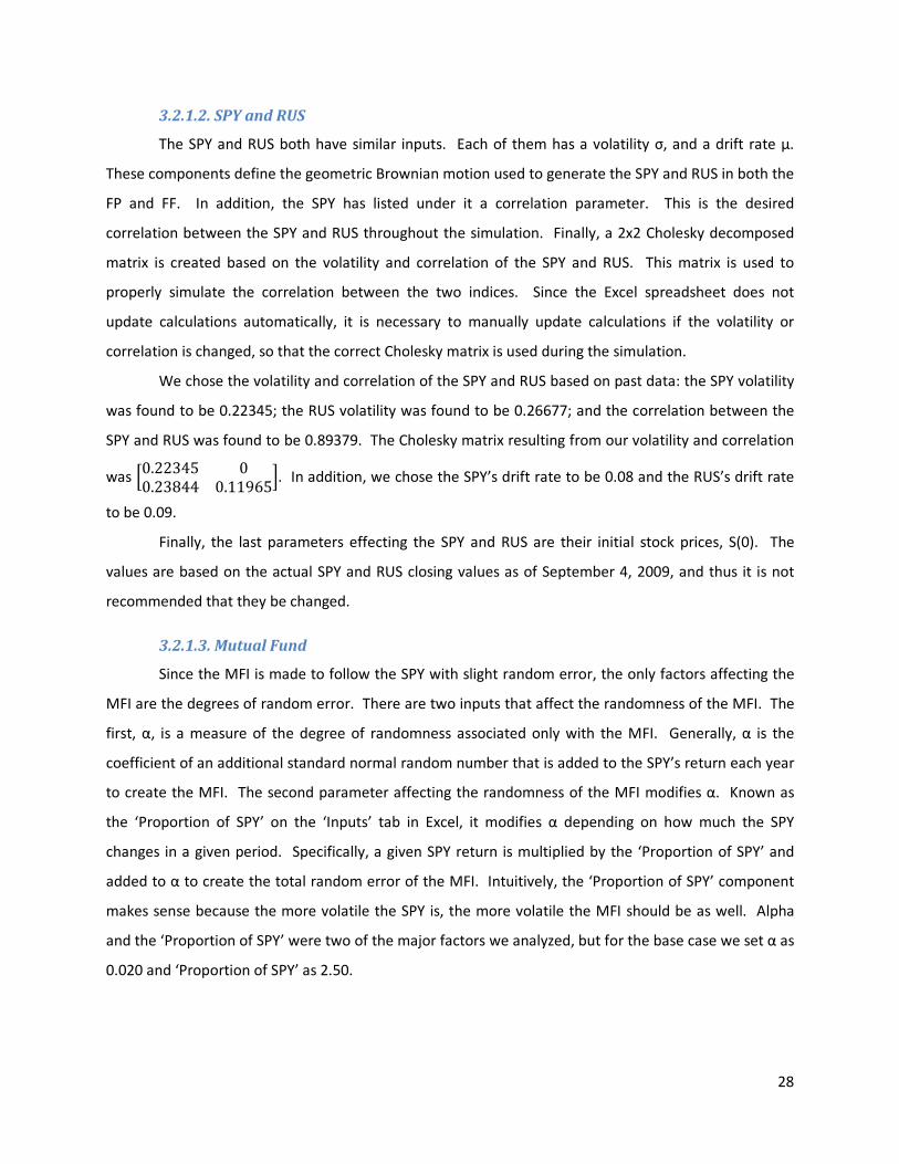
28

3.2.1.2. SPY and RUS

The SPY and RUS both have similar inputs. Each of them has a volatility σ, and a drift rate μ.

These components define the geometric Brownian motion used to generate the SPY and RUS in both the

FP and FF. In addition, the SPY has listed under it a correlation parameter. This is the desired

correlation between the SPY and RUS throughout the simulation. Finally, a 2x2 Cholesky decomposed

matrix is created based on the volatility and correlation of the SPY and RUS. This matrix is used to

properly simulate the correlation between the two indices. Since the Excel spreadsheet does not

update calculations automatically, it is necessary to manually update calculations if the volatility or

correlation is changed, so that the correct Cholesky matrix is used during the simulation.

We chose the volatility and correlation of the SPY and RUS based on past data: the SPY volatility

was found to be 0.22345; the RUS volatility was found to be 0.26677; and the correlation between the

SPY and RUS was found to be 0.89379. The Cholesky matrix resulting from our volatility and correlation

was �0.22345 00.23844 0.11965�. In addition, we chose the SPY’s drift rate to be 0.08 and the RUS’s drift rate

to be 0.09.

Finally, the last parameters effecting the SPY and RUS are their initial stock prices, S(0). The

values are based on the actual SPY and RUS closing values as of September 4, 2009, and thus it is not

recommended that they be changed.

3.2.1.3. Mutual Fund

Since the MFI is made to follow the SPY with slight random error, the only factors affecting the

MFI are the degrees of random error. There are two inputs that affect the randomness of the MFI. The

first, α, is a measure of the degree of randomness associated only with the MFI. Generally, α is the

coefficient of an additional standard normal random number that is added to the SPY’s return each year

to create the MFI. The second parameter affecting the randomness of the MFI modifies α. Known as

the ‘Proportion of SPY’ on the ‘Inputs’ tab in Excel, it modifies α depending on how much the SPY

changes in a given period. Specifically, a given SPY return is multiplied by the ‘Proportion of SPY’ and

added to α to create the total random error of the MFI. Intuitively, the ‘Proportion of SPY’ component

makes sense because the more volatile the SPY is, the more volatile the MFI should be as well. Alpha

and the ‘Proportion of SPY’ were two of the major factors we analyzed, but for the base case we set α as

0.020 and ‘Proportion of SPY’ as 2.50.

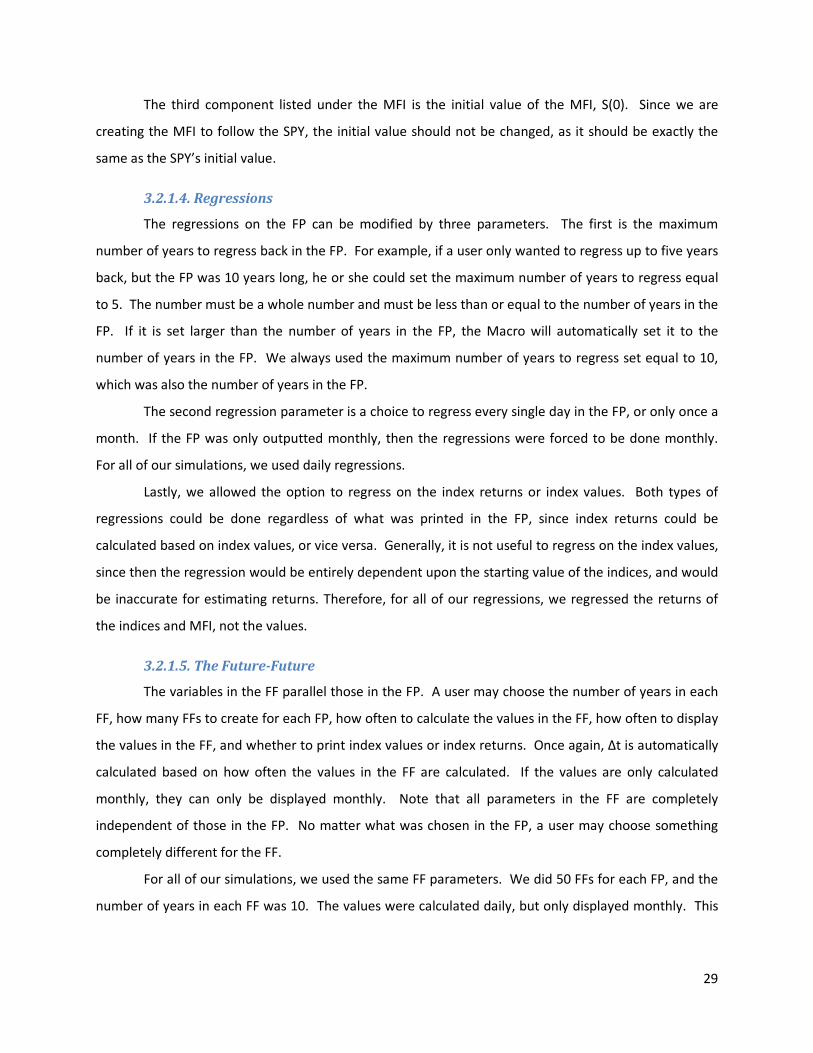
29

The third component listed under the MFI is the initial value of the MFI, S(0). Since we are

creating the MFI to follow the SPY, the initial value should not be changed, as it should be exactly the

same as the SPY’s initial value.

3.2.1.4. Regressions

The regressions on the FP can be modified by three parameters. The first is the maximum

number of years to regress back in the FP. For example, if a user only wanted to regress up to five years

back, but the FP was 10 years long, he or she could set the maximum number of years to regress equal

to 5. The number must be a whole number and must be less than or equal to the number of years in the

FP. If it is set larger than the number of years in the FP, the Macro will automatically set it to the

number of years in the FP. We always used the maximum number of years to regress set equal to 10,

which was also the number of years in the FP.

The second regression parameter is a choice to regress every single day in the FP, or only once a

month. If the FP was only outputted monthly, then the regressions were forced to be done monthly.

For all of our simulations, we used daily regressions.

Lastly, we allowed the option to regress on the index returns or index values. Both types of

regressions could be done regardless of what was printed in the FP, since index returns could be

calculated based on index values, or vice versa. Generally, it is not useful to regress on the index values,

since then the regression would be entirely dependent upon the starting value of the indices, and would

be inaccurate for estimating returns. Therefore, for all of our regressions, we regressed the returns of

the indices and MFI, not the values.

3.2.1.5. The Future-Future

The variables in the FF parallel those in the FP. A user may choose the number of years in each

FF, how many FFs to create for each FP, how often to calculate the values in the FF, how often to display

the values in the FF, and whether to print index values or index returns. Once again, Δt is automatically

calculated based on how often the values in the FF are calculated. If the values are only calculated

monthly, they can only be displayed monthly. Note that all parameters in the FF are completely

independent of those in the FP. No matter what was chosen in the FP, a user may choose something

completely different for the FF.

For all of our simulations, we used the same FF parameters. We did 50 FFs for each FP, and the

number of years in each FF was 10. The values were calculated daily, but only displayed monthly. This

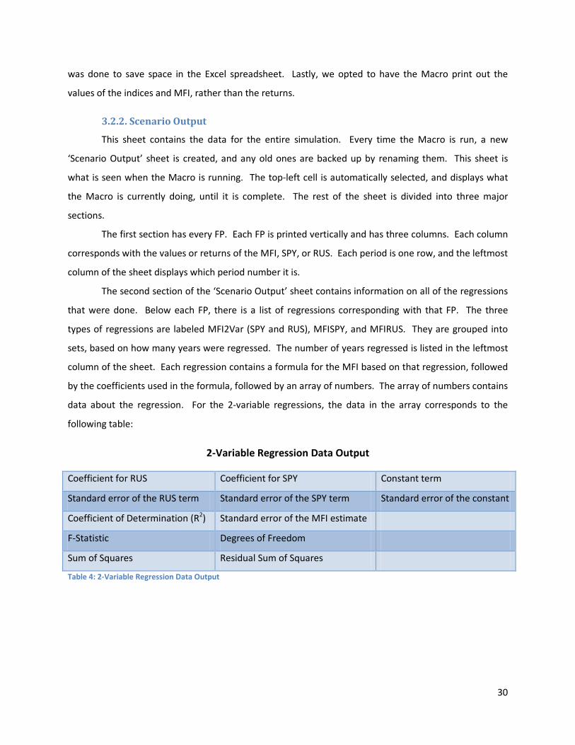
30

was done to save space in the Excel spreadsheet. Lastly, we opted to have the Macro print out the

values of the indices and MFI, rather than the returns.

3.2.2. Scenario Output

This sheet contains the data for the entire simulation. Every time the Macro is run, a new

‘Scenario Output’ sheet is created, and any old ones are backed up by renaming them. This sheet is

what is seen when the Macro is running. The top-left cell is automatically selected, and displays what

the Macro is currently doing, until it is complete. The rest of the sheet is divided into three major

sections.

The first section has every FP. Each FP is printed vertically and has three columns. Each column

corresponds with the values or returns of the MFI, SPY, or RUS. Each period is one row, and the leftmost

column of the sheet displays which period number it is.

The second section of the ‘Scenario Output’ sheet contains information on all of the regressions

that were done. Below each FP, there is a list of regressions corresponding with that FP. The three

types of regressions are labeled MFI2Var (SPY and RUS), MFISPY, and MFIRUS. They are grouped into

sets, based on how many years were regressed. The number of years regressed is listed in the leftmost

column of the sheet. Each regression contains a formula for the MFI based on that regression, followed

by the coefficients used in the formula, followed by an array of numbers. The array of numbers contains

data about the regression. For the 2-variable regressions, the data in the array corresponds to the

following table:

2-Variable Regression Data Output

Coefficient for RUS Coefficient for SPY Constant term

Standard error of the RUS term Standard error of the SPY term Standard error of the constant

Coefficient of Determination (R2) Standard error of the MFI estimate

F-Statistic Degrees of Freedom

Sum of Squares Residual Sum of Squares

Table 4: 2-Variable Regression Data Output

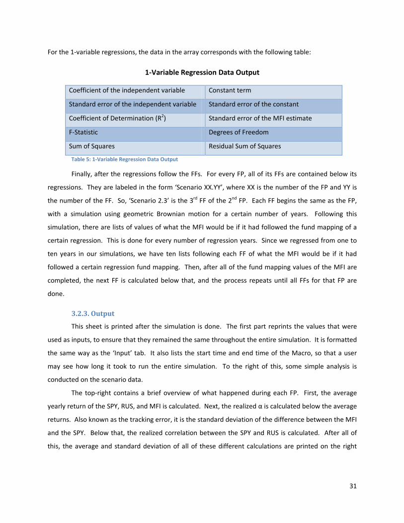
31

For the 1-variable regressions, the data in the array corresponds with the following table:

1-Variable Regression Data Output

Coefficient of the independent variable Constant term

Standard error of the independent variable Standard error of the constant

Coefficient of Determination (R2) Standard error of the MFI estimate

F-Statistic Degrees of Freedom

Sum of Squares Residual Sum of Squares

Table 5: 1-Variable Regression Data Output

Finally, after the regressions follow the FFs. For every FP, all of its FFs are contained below its

regressions. They are labeled in the form ‘Scenario XX.YY’, where XX is the number of the FP and YY is

the number of the FF. So, ‘Scenario 2.3’ is the 3rd FF of the 2nd FP. Each FF begins the same as the FP,

with a simulation using geometric Brownian motion for a certain number of years. Following this

simulation, there are lists of values of what the MFI would be if it had followed the fund mapping of a

certain regression. This is done for every number of regression years. Since we regressed from one to

ten years in our simulations, we have ten lists following each FF of what the MFI would be if it had

followed a certain regression fund mapping. Then, after all of the fund mapping values of the MFI are

completed, the next FF is calculated below that, and the process repeats until all FFs for that FP are

done.

3.2.3. Output

This sheet is printed after the simulation is done. The first part reprints the values that were

used as inputs, to ensure that they remained the same throughout the entire simulation. It is formatted

the same way as the ‘Input’ tab. It also lists the start time and end time of the Macro, so that a user

may see how long it took to run the entire simulation. To the right of this, some simple analysis is

conducted on the scenario data.

The top-right contains a brief overview of what happened during each FP. First, the average

yearly return of the SPY, RUS, and MFI is calculated. Next, the realized α is calculated below the average

returns. Also known as the tracking error, it is the standard deviation of the difference between the MFI

and the SPY. Below that, the realized correlation between the SPY and RUS is calculated. After all of

this, the average and standard deviation of all of these different calculations are printed on the right

32

side. These calculations are mostly for error checking, to make sure that the correlation, MFI random

error, and expected returns were implemented correctly.

Finally, the lower-right portion contains simple analysis of the regression data. It finds the

averages of several key parameters of the regression for each number of years regressed. Specifically,

the average of the coefficients, standard error, and R2 for each type of regression is calculated for each

of the regression years. The last column on the right contains averages among all regression years for

the various parameters.

3.2.4. Graph Data

After the Macro generates the entire simulation, it prints certain data into this sheet that will be

displayed in graphs. In a way, it is an extension of the ‘Output’ tab. It is divided into two main sections:

the top portion has data concerning regression coefficients, and the lower portion contains the

differences between the real MFI and benchmark MFI in the FF.

For the regressions, The Macro looks separately at each coefficient. Each 1-variable regression

has one coefficient, and the 2-variable regressions have 1 SPY coefficient and 1 RUS coefficient. For

each of these four coefficients, the Macro does the same thing. Looking at each year separately, it

analyzes the minimum, first quartile, median, mean, third quartile, and maximum of a coefficient. This

is done for all years of regressions. For example, in our case, since we regressed up to 10 years, we have

10 different sets of regressions to look at for each of the four types of coefficients.

Below the regression analysis are the percentage differences between the benchmarks and the

real values of the MFI. For each of the 30 regressions we performed (three types of regressions times

ten years), the Macro looked at the percentage difference between the real MFI and the value based on

that benchmark every month. The Macro finds the minimum, first quartile, median, mean, third

quartile, and maximum difference every month for each type of regression.

3.2.5. Graphs

The last things that are output by the Macro are the graphs. There are two types of graphs. The

first type of graph shows a scatter plot of the regression coefficients for the various regressions, and the

second type of graph is a line chart displaying the difference between the real MFI and the MFI fund

mapping from the regression.

There are four different graphs showing coefficients. These correspond with the SPY coefficient

from the 2-variable regression, RUS coefficient from the 2-variable regression, the SPY coefficient from

the 1-variable SPY regression, and the RUS coefficient from the 1-variable RUS coefficient. Each graph

33

shows the maximum, third quartile, median, first quartile, and minimum coefficients of the 50 scenarios,

for every number of years regressed. These values are pulled from the ‘Graph Data’ tab, thus the charts

are a graphical representation of the numbers displayed there. For an example of this type of graph, see

Figure 4.

The Macro creates 30 of the second type of graph. Each one of these shows the monthly

maximum, third quartile, median, first quartile, and minimum difference between the real MFI and one

of the proxy MFI fund mappings found via regression. Since there were thirty different regressions

(three types of regressions times ten years), there is a different graph for each one. As before, the data

for these graphs is pulled from the ‘Graph Data’ sheet. See Figure 5 for an example of this type of graph.

34

Figure 4: Example of the first type of chart generated by the Macro

Figure 5: Example of the second type of chart generated by the Macro

-0.10

-0.08

-0.06

-0.04

-0.02

0.00

0.02

0.04

0.06

0.08

0.10

0 1 2 3 4 5 6 7 8 9 10

RUS

Coef

ficie

nt

Years Regressed

RUS Coefficient of 2-Variable Regression

Maximum

3rd Quartile

Median

1st Quartile

Minimum

-60%

-40%

-20%

0%

20%

40%

60%

80%

100%

1 6 11 16 21 26 31 36 41 46 51 56 61 66 71 76 81 86 91 96 101

106

111

116

Perc

ent D

iffer

ence

bet

wee

n M

utua

l Fun

ds

Period

% Difference Between Real MF and 2-VAR MF (10 Year Regression)

Maximum

3rd QuartileMedian

1st QuartileMinimum

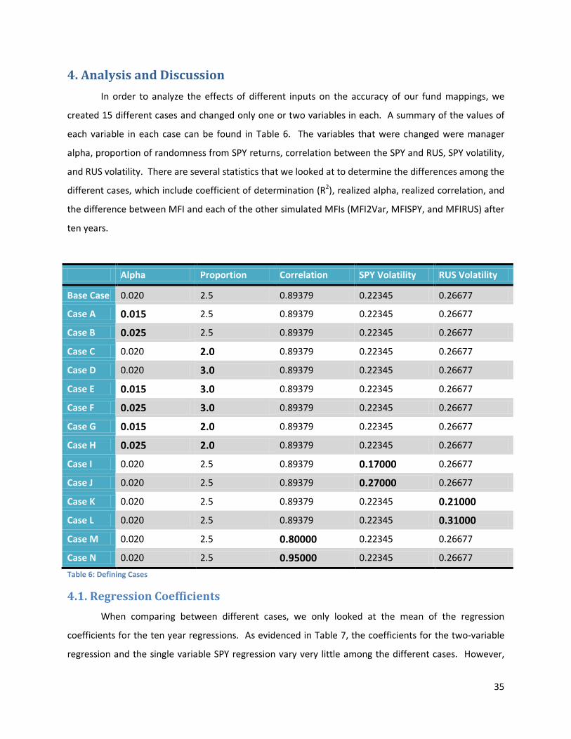
35

4. Analysis and Discussion

In order to analyze the effects of different inputs on the accuracy of our fund mappings, we

created 15 different cases and changed only one or two variables in each. A summary of the values of

each variable in each case can be found in Table 6. The variables that were changed were manager

alpha, proportion of randomness from SPY returns, correlation between the SPY and RUS, SPY volatility,

and RUS volatility. There are several statistics that we looked at to determine the differences among the

different cases, which include coefficient of determination (R2), realized alpha, realized correlation, and

the difference between MFI and each of the other simulated MFIs (MFI2Var, MFISPY, and MFIRUS) after

ten years.

Table 6: Defining Cases

4.1. Regression Coefficients

When comparing between different cases, we only looked at the mean of the regression

coefficients for the ten year regressions. As evidenced in Table 7, the coefficients for the two-variable

regression and the single variable SPY regression vary very little among the different cases. However,

Alpha Proportion Correlation SPY Volatility RUS Volatility

Base Case 0.020 2.5 0.89379 0.22345 0.26677

Case A 0.015 2.5 0.89379 0.22345 0.26677

Case B 0.025 2.5 0.89379 0.22345 0.26677

Case C 0.020 2.0 0.89379 0.22345 0.26677

Case D 0.020 3.0 0.89379 0.22345 0.26677

Case E 0.015 3.0 0.89379 0.22345 0.26677

Case F 0.025 3.0 0.89379 0.22345 0.26677

Case G 0.015 2.0 0.89379 0.22345 0.26677

Case H 0.025 2.0 0.89379 0.22345 0.26677

Case I 0.020 2.5 0.89379 0.17000 0.26677

Case J 0.020 2.5 0.89379 0.27000 0.26677

Case K 0.020 2.5 0.89379 0.22345 0.21000

Case L 0.020 2.5 0.89379 0.22345 0.31000

Case M 0.020 2.5 0.80000 0.22345 0.26677

Case N 0.020 2.5 0.95000 0.22345 0.26677

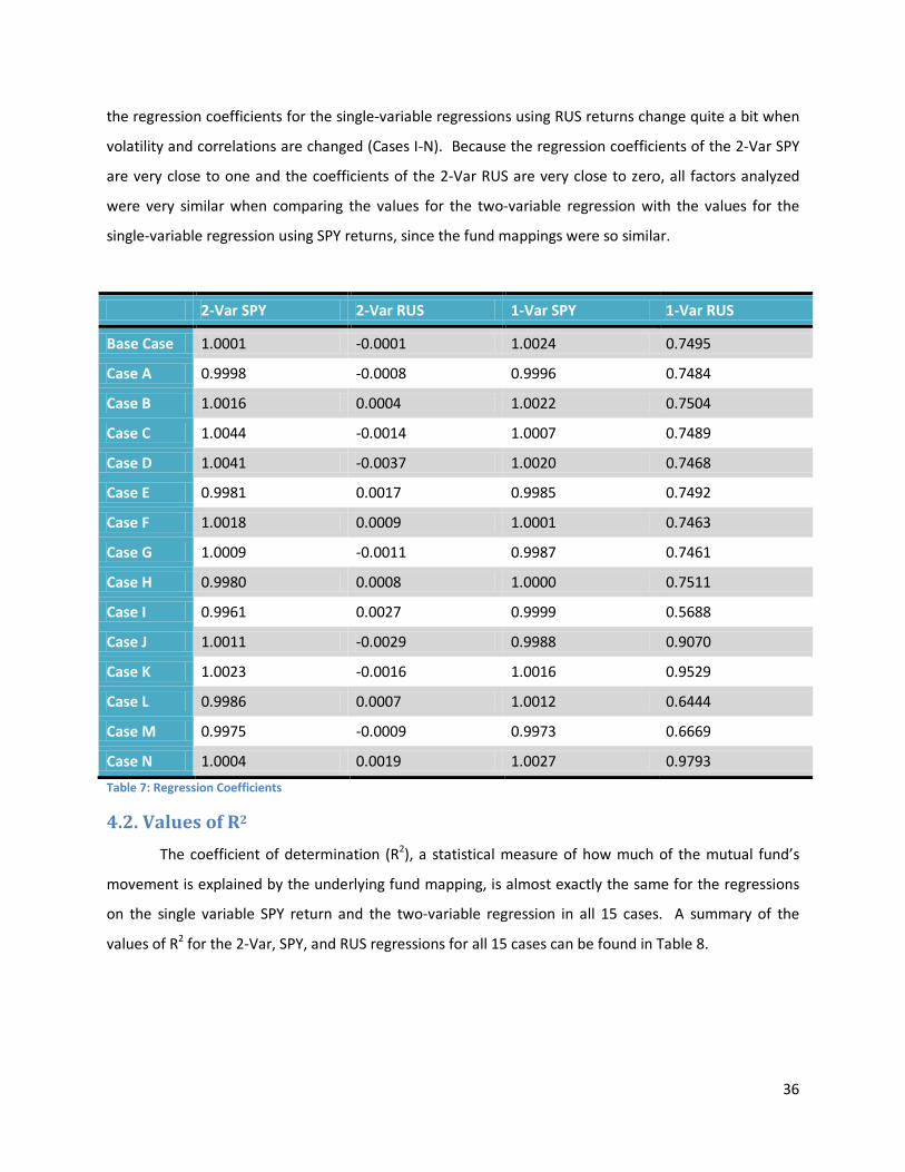
36

the regression coefficients for the single-variable regressions using RUS returns change quite a bit when

volatility and correlations are changed (Cases I-N). Because the regression coefficients of the 2-Var SPY

are very close to one and the coefficients of the 2-Var RUS are very close to zero, all factors analyzed

were very similar when comparing the values for the two-variable regression with the values for the

single-variable regression using SPY returns, since the fund mappings were so similar.

Table 7: Regression Coefficients

4.2. Values of R2

The coefficient of determination (R2), a statistical measure of how much of the mutual fund’s

movement is explained by the underlying fund mapping, is almost exactly the same for the regressions

on the single variable SPY return and the two-variable regression in all 15 cases. A summary of the

values of R2 for the 2-Var, SPY, and RUS regressions for all 15 cases can be found in Table 8.

2-Var SPY 2-Var RUS 1-Var SPY 1-Var RUS

Base Case 1.0001 -0.0001 1.0024 0.7495

Case A 0.9998 -0.0008 0.9996 0.7484

Case B 1.0016 0.0004 1.0022 0.7504

Case C 1.0044 -0.0014 1.0007 0.7489

Case D 1.0041 -0.0037 1.0020 0.7468

Case E 0.9981 0.0017 0.9985 0.7492

Case F 1.0018 0.0009 1.0001 0.7463

Case G 1.0009 -0.0011 0.9987 0.7461

Case H 0.9980 0.0008 1.0000 0.7511

Case I 0.9961 0.0027 0.9999 0.5688

Case J 1.0011 -0.0029 0.9988 0.9070

Case K 1.0023 -0.0016 1.0016 0.9529

Case L 0.9986 0.0007 1.0012 0.6444

Case M 0.9975 -0.0009 0.9973 0.6669

Case N 1.0004 0.0019 1.0027 0.9793

37

Table 8: Average Values of R2

As evidenced in the Table 8, the values of R2 for the 2-Var and SPY regressions are all within a

reasonably small range. The lowest value of R2 is from Case F with a value of 0.9245, where we raised

alpha from 0.020 to 0.025 and we raised the proportion of randomness from the SPY returns from 2.5 to

3.0. This is to be expected because this combination of alpha and proportion allows for the most

randomness among all of the cases. The highest value is from Case G with a value of 0.9670, where we

lowered alpha from 0.020 to 0.015 and lowered the proportion from 2.5 to 2.0. As with the lowest

value, this is to be expected because this combination of alpha and proportion allows for the least

amount of randomness, so MFI follows the SPY more closely and the regression is more accurate. In

general, the values of R2 for the 2-Var and SPY regressions all hover around 0.95, meaning that about

95% of the momentum of MFI can be explained by SPY alone or by the SPY and RUS combined. When

there is a difference between the value of R2 for the 2-Var and RUS regressions, it is a difference of only

about 0.0001, which may be a rounding error. Because there is such a high correlation between the SPY

2-Var SPY RUS

Base Case 0.9485 0.9485 0.7580

Case A 0.9560 0.9559 0.7635

Case B 0.9391 0.9391 0.7532

Case C 0.9600 0.9600 0.7661

Case D 0.9345 0.9345 0.7457

Case E 0.9429 0.9428 0.7539

Case F 0.9245 0.9244 0.7398

Case G 0.9670 0.9670 0.7712

Case H 0.9518 0.9517 0.7606

Case I 0.9363 0.9362 0.7461

Case J 0.9538 0.9357 0.7630

Case K 0.9481 0.9480 0.7567

Case L 0.9473 0.9473 0.7567

Case M 0.9475 0.9474 0.6073

Case N 0.9483 0.9483 0.8557

38

and MFI returns, adding the RUS returns in does not help explain the movement of MFI. This means

that the SPY already explains the movement well enough such that adding the RUS has no additional

positive effect. Effectively, the two fund mappings are virtually identical.

Because the RUS is not the proper benchmark for MFI, the values of R2 are lower when looking

at the RUS fund mapping. Generally, the RUS accounted for about 75% of the movement of the SPY,

since the values of R2 were generally around 0.75. This value is much lower than the R2 of 0.95 in the

other types of regressions because the RUS is not the proper benchmark. In addition, the values of R2

for the RUS regressions have a much larger range than the values for the other types of regressions.

However, this is mostly because of two outliers, Case M and Case N. These are the cases where the

correlation between SPY and RUS returns is changed. Changing the correlation has the largest impact on

the RUS regression because changing the correlation between RUS and SPY changes the correlation

between MFI and RUS returns but not between MFI and SPY returns. Aside from those two outliers, the

highest and lowest values of R2 for the RUS regressions correspond directly with the highest and lowest

values of R2 for the 2-Var and SPY regressions.

4.3. Realized Alpha and Correlation

Realized alpha, or tracking error, is the standard deviation of the difference between MFI and

SPY. It is the average of the observed values of manager alpha throughout all 50 FP scenarios, and takes

into account both the manager alpha and the ‘Proportion of SPY’ parameters. The Standard Deviation of

Tracking Error in Table 9 is the standard deviation of the realized alphas of all 50 FP scenarios. Average

realized correlation was calculated mostly in order to ensure that our calculations were being done

correctly as a form of error checking, and the standard deviation across all 50 FP scenarios is also shown

in Table 9.

The values of the realized alpha are all within a relatively close range. They tended to be

between 5.00% and 5.50%, except in exceptional cases. The lowest value comes from Case G with a

value of 4.13%, because in Case G, we lowered the manager alpha from 0.020 to 0.015 and lowered the

proportion from 2.5 to 2.0, which limited the amount of randomness. This, in turn, lowered the

difference between the MFI and SPY returns. The highest value of realized alpha came from Case F with

a value of 6.41%. This also is not surprising because in Case F we raised manager alpha from 0.020 to

0.025 and raised the proportion from 2.5 to 3.0, which allowed more randomness than any other case.

These results are not extraordinary, and serve more as a confirmation that the implementation of the

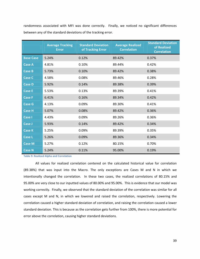
39

randomness associated with MFI was done correctly. Finally, we noticed no significant differences

between any of the standard deviations of the tracking error.

Average Tracking

Error Standard Deviation

of Tracking Error Average Realized

Correlation

Standard Deviation of Realized Correlation

Base Case 5.24% 0.12% 89.42% 0.37%

Case A 4.81% 0.10% 89.44% 0.42%

Case B 5.73% 0.10% 89.42% 0.38%

Case C 4.58% 0.08% 89.46% 0.28%

Case D 5.92% 0.14% 89.38% 0.39%

Case E 5.53% 0.13% 89.39% 0.41%

Case F 6.41% 0.16% 89.34% 0.42%

Case G 4.13% 0.09% 89.30% 0.41%

Case H 5.07% 0.08% 89.42% 0.36%

Case I 4.43% 0.09% 89.26% 0.36%

Case J 5.93% 0.14% 89.42% 0.34%

Case K 5.25% 0.09% 89.39% 0.35%

Case L 5.26% 0.09% 89.36% 0.34%

Case M 5.27% 0.12% 80.15% 0.70%

Case N 5.24% 0.11% 95.00% 0.19%

Table 9: Realized Alpha and Correlation

All values for realized correlation centered on the calculated historical value for correlation

(89.38%) that was input into the Macro. The only exceptions are Cases M and N in which we

intentionally changed the correlation. In these two cases, the realized correlations of 80.15% and

95.00% are very close to our inputted values of 80.00% and 95.00%. This is evidence that our model was

working correctly. Finally, we observed that the standard deviation of the correlation was similar for all

cases except M and N, in which we lowered and raised the correlation, respectively. Lowering the

correlation caused a higher standard deviation of correlation, and raising the correlation caused a lower

standard deviation. This is because as the correlation gets further from 100%, there is more potential for

error above the correlation, causing higher standard deviations.

40

4.4. Ending Difference between MFI and MFI2Var

Table 10 shows the 25th percentile, 75th percentile, median, and interquartile range (75th

percentile minus 25th percentile) of the ending difference between the MFI and MFI2Var returns at the

end of the ten-year FF.

25th Percentile Median 75th Percentile Interval Length

Base Case -10.43% 0.30% 12.59% 23.02%

Case A -10.92% -1.02% 9.88% 20.80%

Case B -7.89% 0.24% 8.94% 16.83%

Case C -9.10% 0.49% 10.97% 20.07%

Case D -12.40% -0.14% 13.47% 25.87%

Case E -11.76% -0.15% 12.09% 23.85%

Case F -12.51% 0.18% 14.25% 26.76%

Case G -8.64% 0.02% 10.12% 18.76%

Case H -9.55% 0.04% 12.17% 21.72%

Case I -10.16% -0.67% 9.36% 19.52%

Case J -12.03% -1.17% 10.05% 22.08%

Case K -9.64% 1.70% 13.85% 23.49%

Case L -8.86% -0.52% 8.09% 16.95%

Case M -12.15% -0.54% 11.83% 23.98%

Case N -11.30% -0.73% 11.56% 22.86%

Table 10: Difference between MFI and MFI2Var

In general, there are not any unexpected results. The median is around 0% for all cases,

meaning that on average there is no difference between the MFI and the 2-Var fund mapping after ten

years. In other words, the fund mapping is accurate on average. This is corroborated by the values of R2

that we found for the 2-Var regression, which were all around 0.95 and signaled that the regression was

accurate. The 25th and 75th percentiles are generally around -10% and 10% respectively, meaning that

about 50% of the time, the fund mapping will be off by less than 10%. The other 50% of the time, there

would be even more error. This shows the effect of basis risk; there may be certain situations when

things simply go awry due to unexpected problems, when in other situations there is a positive

outcome, even with the same inputs.

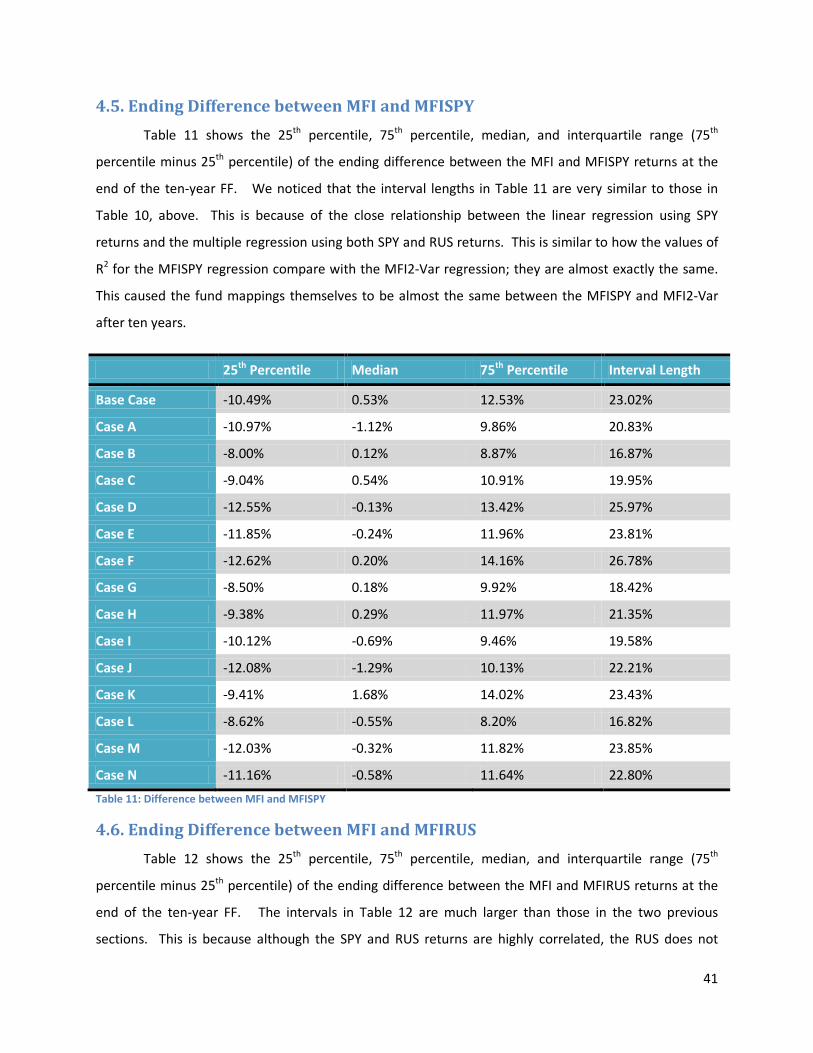
41

4.5. Ending Difference between MFI and MFISPY


percentile minus 25th percentile) of the ending difference between the MFI and MFISPY returns at the

end of the ten-year FF. We noticed that the interval lengths in Table 11 are very similar to those in

Table 10, above. This is because of the close relationship between the linear regression using SPY

returns and the multiple regression using both SPY and RUS returns. This is similar to how the values of

R2 for the MFISPY regression compare with the MFI2-Var regression; they are almost exactly the same.

This caused the fund mappings themselves to be almost the same between the MFISPY and MFI2-Var

after ten years.


Base Case -10.49% 0.53% 12.53% 23.02%

Case A -10.97% -1.12% 9.86% 20.83%

Case B -8.00% 0.12% 8.87% 16.87%

Case C -9.04% 0.54% 10.91% 19.95%

Case D -12.55% -0.13% 13.42% 25.97%

Case E -11.85% -0.24% 11.96% 23.81%

Case F -12.62% 0.20% 14.16% 26.78%

Case G -8.50% 0.18% 9.92% 18.42%

Case H -9.38% 0.29% 11.97% 21.35%

Case I -10.12% -0.69% 9.46% 19.58%

Case J -12.08% -1.29% 10.13% 22.21%

Case K -9.41% 1.68% 14.02% 23.43%

Case L -8.62% -0.55% 8.20% 16.82%

Case M -12.03% -0.32% 11.82% 23.85%

Case N -11.16% -0.58% 11.64% 22.80%

Table 11: Difference between MFI and MFISPY

4.6. Ending Difference between MFI and MFIRUS


percentile minus 25th percentile) of the ending difference between the MFI and MFIRUS returns at the

end of the ten-year FF. The intervals in Table 12 are much larger than those in the two previous

sections. This is because although the SPY and RUS returns are highly correlated, the RUS does not

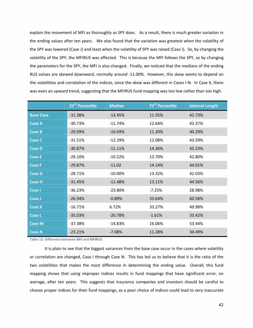
42

explain the movement of MFI as thoroughly as SPY does. As a result, there is much greater variation in

the ending values after ten years. We also found that the variation was greatest when the volatility of

the SPY was lowered (Case J) and least when the volatility of SPY was raised (Case I). So, by changing the

volatility of the SPY, the MFIRUS was affected. This is because the MFI follows the SPY, so by changing

the parameters for the SPY, the MFI is also changed. Finally, we noticed that the medians of the ending

RUS values are skewed downward, normally around -11.00%. However, this skew seems to depend on

the volatilities and correlation of the indices, since the skew was different in Cases I-N. In Case K, there

was even an upward trend, suggesting that the MFIRUS fund mapping was too low rather than too high.


Base Case -31.38% -13.45% 11.35% 42.73%

Case A -30.73% -11.74% 12.64% 43.37%

Case B -29.09% -10.69% 11.20% 40.29%

Case C -31.51% -12.29% 12.08% 43.59%

Case D -30.87% -11.11% 14.36% 45.23%

Case E -29.10% -10.22% 13.70% 42.80%

Case F -29.87% -11.02 14.14% 44.01%

Case G -28.71% -10.00% 13.32% 42.03%

Case H -31.45% -11.48% 13.11% 44.56%

Case I -36.23% -23.80% -7.25% 28.98%

Case J -26.94% -0.89% 33.64% 60.58%

Case K -16.71% 6.72% 33.27% 49.98%

Case L -35.03% -20.78% -1.61% 33.42%

Case M -37.38% -14.83% 16.06% 53.44%

Case N -23.21% -7.08% 11.28% 34.49%

Table 12: Difference between MFI and MFIRUS

It is plain to see that the biggest variances from the base case occur in the cases where volatility

or correlation are changed, Case I through Case N. This has led us to believe that it is the ratio of the

two volatilities that makes the most difference in determining the ending value. Overall, this fund

mapping shows that using improper indices results in fund mappings that have significant error, on

average, after ten years. This suggests that insurance companies and investors should be careful to

choose proper indices for their fund mappings, as a poor choice of indices could lead to very inaccurate

43

fund mappings. One important statistic to pay attention to is R2. If R2 is close to one, the fund mapping

can be expected to be very accurate, but if it is further from one, the fund mapping can be expected to

be more inaccurate.

44

5. Conclusions and Recommendations

Within this section we will discuss the conclusions and recommendation of our research. We

will begin with an analysis of our results and interpretations of their meaning. Following this, we will

then discuss ways to improve our model and other suggestions for future research. Finally, we will

conclude with a summary of our research.

5.1. Conclusions

After analyzing the results of many different cases and situations, we have come up with some

conclusions about the research. These conclusions revolve around several different themes, such as

correlation, multicollinearity, volatility, and regressions over different periods of time.

5.1.1. Correlation

One interesting observation that we made during the simulations was the effect of correlation

on the fund mapping accuracy. When the correlation between the SPY and RUS was raised or lowered,

there was no effect on the 1-variable SPY regression or the 2-variable regression. However, the

accuracy of the 1-variable RUS regression was directly impacted by the correlation. Precisely, when the

correlation was lowered, the 1-variable RUS coefficient became further away from 1, the R2 was lower,

and the fund mapping was less accurate. On the other hand, when the correlation was raised, the

coefficient was closer to 1 (and thus more accurate), the R2 was higher, and the fund mapping was more

accurate. Therefore, the correlation between indices affects the accuracy of fund mappings when using

improper indices. However, when the chosen indices sufficiently explained the movements of the

mutual fund, and thus a proper benchmark was found, the correlation had little effect on the outcome

of fund mapping accuracy. Additionally, indices having high correlations may be falsely estimated as

being the actual benchmarks, even if though the real benchmark is a different highly correlated index.

This error is known as multicollinearity.

5.1.2. Multicollinearity

One issue that could have potentially affected the results was multicollinearity. Multicollinearity

occurs when two independent variables in a multiple regression are highly correlated. Although we

anticipated multicollinearity to be a source of error, we did not find this to be the case. Even with highly

correlated indices (as in Case N with correlation set to 0.95), multicollinearity did not seem to occur.

Even though the RUS and SPY were highly correlated, the 2-variable regression still depended mostly on

the SPY and was unaffected by the RUS. If multicollinearity had occurred, we would have seen a large

45

mismatch between the MFISPY and the MFI2-Var, due to the high correlation between the SPY and RUS

affecting the fund mappings. Since this did not occur, multicollinearity was not an issue when using this

model. However, it may be important to recognize multicollinearity in future research when using

different models or indices, and to further study the effect of multicollinearity on fund mappings.

5.1.3. Volatility

From Cases I and J, in which the SPY volatility was changed, the biggest effect was actually the

accuracy of the RUS regressions. Intuitively, this may not make sense because changing the SPY

volatility should not change the RUS’s accuracy. However, the reason is because the accuracy of the

RUS depends entirely on the difference between the volatility of the SPY and RUS. Putting everything

together from Cases I, J, K, L, and the base case, the effect of volatilities on the accuracy of the RUS

regression is in Table 13.

Case I Case L Base Case Case J Case K

SPY Volatility 0.17000 0.22345 0.22345 0.27000 0.22345

RUS Volatility 0.26677 0.31000 0.26677 0.26677 0.21000

(SPY vol)/(RUS vol) 0.63725 0.72081 0.83761 1.01211 1.06405

Median RUS regression error -23.78% -20.81% -13.43% -0.89% 6.70%

Table 13: Effect of volatility on improper fund mappings

If we compare the ratio of SPY volatility and RUS volatility to the accuracy of the RUS fund

mapping, we can see that the average error of the RUS is directly related to the ratio of the SPY volatility

to the RUS volatility. Notice that as the ratio of SPY volatility to RUS volatility increases, the median

error of the RUS-only regression after 10 years increases. When the two volatilities are almost equal,

the error is about zero (Case J). Therefore, we can conclude that the ratio of the index volatilities

directly impacts the accuracy of benchmarks that use improper indices. Therefore, investors should be

mindful of the volatilities of indices that they choose to use for fund mappings. If the volatilities vary

greatly, there may be errors due to certain indices being more or less volatile than the true benchmark,

resulting in errors due to this difference.

5.1.4. Regression Periods

One goal of the project was to see if there was any change when regressing a different number

of years into the past. Throughout all cases, the number of years regressed seemed to have very little

effect on any of the data that we analyzed, including R2 and fund mapping accuracy. The only difference

occurred in the regression coefficients. Generally, the more years regressed, the closer the coefficients

46

were to what the true fund mapping should be, and the lower the interquartile range (error) of the

coefficients was. However, this did not have any significant effect on any other data. We believe that

this is because we have used only static volatilities, correlations, and other parameters that do not

change at all throughout our entire simulation process. Had we had time to improve our model so that

volatility and correlation were stochastic, it would most likely have resulted in visibly different results

among the different regression periods analyzed. It may have also made a difference if we had

regressed monthly (or some other quantity of time) as opposed to daily. With daily regressions, there is

a large amount of data to utilize. Therefore, even with only a one year regression, the regression will be

very accurate. However, in the real world, historical data will always be present to use for regressions,

so it may be more realistic to simply use all data that is available.

5.1.5. How Our Results Relate to Active Management and Basis Risk

Our research does not take into account all aspects of basis risk. Since we know the exact

benchmark, we do not have to worry about basis risk arising from choosing an incorrect proxy hedge or

fund mapping. We also eliminated the possibility that the manager changed his strategy because we

controlled all of the variables. Therefore, we only were analyzing the risk arising from the manager

trying to outperform the benchmark. We found that, using our static model, this type of basis risk

would be nothing on average. However, because the average is just an average and does not always

occur, there may be significant error in some cases. This is the basis risk. Sometimes the mutual may

outperform its fund mapping, or sometimes it may underperform its fund mapping, due to the random

error of a manager trying to outperform the benchmark. Although we have not found a way to

eliminate basis risk which would be impossible, we can suggest some ways to minimize it. One way to

minimize basis risk would be to ensure that the indices chosen for the fund mapping are representative

of the mutual fund. As our data had shown, using improper indices results in a large error and volatility

of possible outcomes. Therefore, insurance companies and investors should pay attention to statistical

measures such as R2 in order to obtain the most accurate fund mapping. In addition, the volatilities of

the indices may have some effect on the mean accuracy of the fund mappings. Asset managers should

ensure that they choose indices with similar volatilities to the mutual fund itself in order to minimize this

type of error. These suggestions are only a couple of ways to minimize one type of basis risk, and there

may be many more. Future research may be able to find ways in order to further minimize basis risk.

47

5.2. Improvements and Future Research

Our conclusions make it clear that many improvements can be made in order to further study

the effects of basis risk and active management on fund mappings. We hypothesize that one of the

greatest limitations of our research is the model itself. Therefore, we propose a variety of ideas and

techniques that may be implemented by future researchers in order to make the model more versatile.

With a better model, more conclusions may be able to be made about basis risk and the accuracy of

fund mappings.

5.2.1. Creating Stochastic Parameters

Throughout our simulations, we used a constant mean, volatility, and correlation in the

geometric Brownian motion. This is not very realistic. In reality, the drift rate, volatility, and correlation

of indices are constantly changing. Assuming that they remain constant for years is a large assumption

and makes our model less applicable to the real world. Future research might look into creating

stochastic volatilities and correlation when modeling indices, and how they affect the accuracy of

benchmarks and manager tracking error.

For example, it is questionable to assume that indices correlated in the past will continue to be

correlated in the future. If the correlation is changing, it will be most similar to the historical correlation

early on, and then begin to drift as time passes. Therefore, a person creating stochastic correlation

might want to start with a correlation similar to the historical correlation, and then allow the correlation

to decrease or increase depending on various market factors. For example, correlation between indices

tends to be highest when there are sharp gains or losses in the market. Consequently, the correlation

may be made higher when the absolute returns are very high for a long period of time, and be made

lower when the returns are closer to zero.

In addition, market volatility changes over time. This is evidenced by the fact that the market

moves more severely over some periods than it does over others. It would be interesting to study the

effects of having one volatility in the FP, and then a different volatility (or correlation) in the FF. Or, the

volatility estimate could change based on the observed volatility in the past year during the simulation,

as if a company kept updating their simulation with the most recent data.

By implementing these stochastic volatilities and correlations, our model for equity returns may

become more applicable to the real world. Although we cannot anticipate all factors that may affect the

market in the future, improving the model would at least account for certain behaviors. Therefore,

48

refining the stochastic processes is one of the most fundamental tasks that future researchers should

implement.

5.2.2. More Scenarios

While working with Excel 2003, we were able to generate 50 different scenarios for a 10 year

period. However, we believe that using a larger program and more scenarios may further confirm the

conclusions of our research. Using a larger spreadsheet, such as Excel 2007, would increase available

space in order to run more scenarios and ensure more confidence with our results. Another method

that could potentially provide the simulation with more scenarios would be to use variance reduction

techniques.

One example of a variance reduction technique is using antithetic random numbers. For

example, if we have a random sample of n=2, using a random number U1, we can define U2=1-U1. In our

case we had 50 scenarios (with 50 random numbers), and if we chose to use the antithetic random

number technique, we could have produced twice as many random numbers and therefore twice as

many scenarios (McLeish, 2005). Another variance reduction technique is Importance Sampling. When

using this approach, the simulations are performed on a conditional distribution rather than the original

distribution, and may be desirable if the strike price is significantly above or below the market price

(Cvitanic & Zapatero, 2004).

5.2.3. Adding more indices

After performing our calculations, we found that the SPY and RUS were highly correlated and

using these two indices to create fund mappings gave us results we had originally hypothesized. After

further analysis, we believe that using more than two indices would have provided us with more

diversified and realistic results. In order for our team to use more indices, we would have had to

decrease the number of scenario outputs due to limited space available in Excel 2003. We also would

have had to apply Cholesky decomposition when performing the geometric Brownian motion, which

would have been very computationally expensive.

Generally, portfolios are more diversified and the weights within the portfolio do not normally

only follow two indices. Therefore, if we were to use more indices, then the benchmark would be more

practical and the weighting options would have developed into a more real world situation.

Furthermore, introducing more indices could have given our team a chance to experiment with how

volatile our fund mapping could be. This would include introducing securities that were either very risky

or very conservative, giving us the chance to see how the benchmark would be affected by this change.

49

Moreover, this could result in assorted correlation and experimenting with these combinations could

give more insight to what techniques are efficient. International indices could also be of interest, since

they tend to be very uncorrelated to U.S. indices and have different market factors effecting them.

5.2.4. Choice of Means for SPY and RUS

Calculating the historical mean returns for the SPY and RUS resulted in -1.60% and 3.59% annual

drift rates, respectively. Most of the time, annual returns are not this low, but due to the market decline

in recent years the annual returns are sometimes below zero. If we were to use these means in our

simulation it would have produced an inaccurate representation of long-term market tendencies;

therefore, we decided to use means that were more appropriate for the purpose of our study. Since the

Russell 2000 is a broader index with generally more risk, we chose the mean to equal 9.00% and the S&P

500 to equal 8.00%. We believe that choosing annual returns that accurately represented historical data

would have provided us with more precise results. Another recommendation would be to research how

the annual returns have changed in previous market declines and make valid assumptions based on

historical data. A third possible option is to have the mean return constantly changing to replicate a

more real world situation. In reality, the mean of the stock return is the drift rate and keeping it

constant is an unreliable assumption when developing the simulation. By implementing these ideas,

future research could provide a more secure and dependable fund mapping.

5.3. Final Conclusions

Although we identified sources of basis risk and parameters that may affect basis risk, we did

not conclude that there are problems with the hedging procedures currently in use. In general, the

regressions created fund mappings that were accurate, even when using some improper indices. If we

were to use stochastic parameters, we believe this would have yielded more realistic results.

Furthermore, creating a more diversified portfolio which would include various indices would also

provide our project with more realistic results. More research should be done using the

recommendations we have made in this section in order to further validate the fund mapping

procedure. We hope that by continuing research on the effects and sources of basis risk, insurance

companies and asset managers will eventually be able to improve their investment strategy and

performance, and reduce the risk associated with variable annuities and mutual funds.

50

Bibliography

Active Alpha and Beyond. (2009). Retrieved December 11, 2009, from Goldman Sachs Asset Management: http://www2.goldmansachs.com/gsam/education/USIalpha.html

Active Management. (2009). Retrieved December 8, 2009, from Investopidia: http://www.investopedia.com/terms/a/activemanagement.asp

Banks, E. (2004). Alternative Risk Transfer : Integrated Risk Management Through Insurance, Reinsurance, and the Capital MarketsAlternative Risk Transfer : Integrated Risk Management Through Insurance, Reinsurance, and the Capital Markets. John Wiley & Sons, Inc.

Benchmark. (2009). Retrieved December 8, 2009, from Investopedia: http://www.investopedia.com/terms/b/benchmark.asp

Briere-Giroux, G. (2009, 12 10). Personal Communication. (G. Fredricks, E. Ingalls, & A. McAlister, Interviewers)

Chincarini, L. B., & Kim, D. (2006). Quantitative Equity Portfolio Management. McGraw-Hill Companies, The.

Chriss, N. A. (1996). Black Scholes and Beyond : Option Pricing Models. McGraw-Hill Companies, The .

Corporate Bonds. (2009). Retrieved December 11, 2009, from Investor Words: http://www.investorwords.com/1131/corporate_bond.html

Correlation. (2009). Retrieved December 8, 2009, from Investopedia: http://www.investopedia.com/terms/c/correlation.asp

Correlation Coefficient. (2009). Retrieved December 8, 2009, from Investopedia: http://www.investopedia.com/terms/c/correlationcoefficient.asp

Crouhy, M., Galai, D., & Mark, R. (2001). Risk Management. McGraw-Hill Companies, The.

Curtis, C. E. (2001). Pay Me in Stock Options : Manage the Options You Have, Win the Options You Want . John Wiley & Sons, Inc.

Cvitanic, J., & Zapatero, F. (2004). Introduction to the Economics and Mathematics of Financial Markets. MIT Press.

Dash, J. W. (2004). Quantitative Finance and Risk Management : A Physicist's Approach. World Scientific Publishing Company, Inc.

Finance, B. I. (2005). Boston Institute of Finance Mutual Fund Advisor Course : Series 6 and Series 63 Test Prep. Boston: John Wiley & Sons, Incorporated .

51

Fundamental Law of Active Management. (2007, August 20). Retrieved November 18, 2009, from Financial Education: http://financial-education.com/2007/08/20/fundamental-law-of-active-management/

Grinold, R. C., & Kahn, R. N. (2000). Active Portfolio Management: A Quantitative Approach for Providing Superior Returns and Controlling Risk. McGraw Hill.

Haugh, M. (2004). The Monte Carlo Framework, Examples from Finance and Generating Correlated Random Variables. Retrieved November 30, 2009, from Columbia: http://www.columbia.edu/~mh2078/MCS04/MCS_framework_FEegs.pdf

Hedges, J. R. (2004). Hedges on Hedge Funds : How to Successfully Analyze and Select an Investment. ohn Wiley & Sons, Inc.

Hirt, G. A., & Block, S. B. (2004). Managing Investments. McGraw Hill Companies, The.

Horcher, K. A. (2005). Essentials of Financial Risk Management. John Wiley & Sons, Inc.

Hull, J. C. (2006). Options, Futures, and Other Derivatives. Upper Saddle River: Pearson Education, Inc.

Investment Company Fact Book. (2009). Retrieved October 5, 2009, from The Investment Company Institute: http://ici.org/pdf/2009_factbook.pdf

Investopedia. (2009). Retrieved September 17, 2009, from Guarantee MinimumWithdrawal Benefit: guaranteed minimum death benefit (GMDB),

Kimmel, P. T., Bullen, S., & Green, J. (2004). Excel 2003 VBA Programmer's Reference. John Wiley & Sons, Incorporated.

Levinson, M. (2005). Guide to Financial Markets. Profile Books Limited.

Lhabitant, F.-S. (2004). Hedge Funds : Quantitative Insights. John Wiley & Sons, Inc.

Lim, P. (2005). Investing Demystified. McGraw-Hill Companies, The .

Linear Regression. (1997-1998). Retrieved November 30, 2009, from The Department of Statistics at Yale University: http://www.stat.yale.edu/Courses/1997-98/101/linreg.htm

Litterman, B. (2005). Active Alpha Investing. Retrieved December 11, 2009, from Goldman Sachs: http://www2.goldmansachs.com/ideas/investment-insights/beyond-active-alpha.pdf

McLeish, D. L. (2005). Monte-Carlo Simulations and Finance. John Wiley & Sons, Inc.

Multiple Regression. (2008). Retrieved 29 2009, 2009, from Electronic Textbook StatSoft: http://www.statsoft.com/TEXTBOOK/stmulreg.html

Mutual Funds. (2007, May 14). Retrieved October 2, 2009, from U.S. Securities and Exchange Commision: http://www.sec.gov/answers/mutfund.htm

52

Poterba, J. M. (Ed.). (2006). Tax Policy and the Economy (Vol. 20). MIT Press.

Regression. (2009). Retrieved December 8, 2009, from Investopedia: http://www.investopedia.com/terms/r/regression.asp

SPY - S&P Dep Receipts. (2009). Retrieved 09 04, 2009, from Yahoo! Finance: http://finance.yahoo.com/q?s=spy

Strike Price. (2009). Retrieved December 9, 2009, from Investopedia: http://www.investopedia.com/terms/s/strikeprice.asp

Tracking Error. (2009). Retrieved December 8, 2009, from Investopedia: http://www.investopedia.com/terms/t/trackingerror.asp

Treasury Direct. (2008). Retrieved October 27, 2009, from Saving Bond Sales: http://www.treasurydirect.gov/indiv/research/history/history_sbsales.htm

Variable Annuites: What you should know. (2009, April 28). Retrieved September 17, 2009, from U.S. Securities and Exchange Commision: http://www.sec.gov/investor/pubs/varannty.htm

Wolfinger, M. (2005). Create Your Own Hedge Fund: Increase Profits and Reduce Risk with ETF's and Options. John Wiley & Sons, Inc.

Wolfram MathWorld. (2009). Retrieved December 8, 2009, from Covariance: http://mathworld.wolfram.com/Covariance.html

Wyss, O. (2001). Fundamentals of the Stock Market. McGraw-Hill Professional Book Group.

53

Appendix A: Sponsor Information

Towers, Perrin, Foster, and Crosby (TPF&C) was incorporated in 1934. Their predecessor, Henry

W. Brown Co. can be traced back to 1817. Today, Towers Perrin is a global firm with 41 offices open

outside the United States, 34 offices open within the United States and 16 alliances located around the

world. Towers Perrin serves clients that represent 75% of the world’s 500 largest companies and 75% of

the companies located on the list of U.S. Fortune 1000 companies. They define themselves as a firm

who helps organizations to improve performance through effective people, risk and financial

management. Their Mission Statement is as follows:

“To make significant contributions to improving our clients' business performance ―

through our unique combination of talent, expertise and commitment ― thereby

creating value for our stakeholders”.

Towers Perrin’s services include: Actuarial consulting, Enterprise risk & capital management,

Executive compensation, Financial modeling software solutions, Health & welfare consulting, Human

resources function effectiveness, Insurance consulting, Mergers & acquisitions, Reinsurance, Research &

surveys, Retirement risk, Risk financing and transfer, Total rewards effectiveness, and Talent

management.

54

Appendix B: Acronyms

BC: Breadth Coefficient

DC: Direct Contribution

FP: Future-Past

FF: Future-Future

GMAB: Guaranteed Minimum Accumulation Benefit

GMDB: Guaranteed Minimum Death Benefit

GMIB: Guaranteed Minimum Income Benefit

GMWB: Guaranteed Minimum Withdrawal Benefit

IC: Information Coefficient

IR: Information Ratio

IRA: Individual Retirement Account

MFI: Mutual Fund Incorporated, our created mutual fund

MFI2Var: Predicted mutual fund using two-variable regression

MFISPY: Predicted mutual fund regressed against SPY returns

MFIRUS: Predicted mutual fund regressed against RUS returns

RUS: Russell 2000 index

SPY: S&P 500 yield index

TPF&C: Towers, Perrin, Foster, and Crosby

VA: Variable Annuity

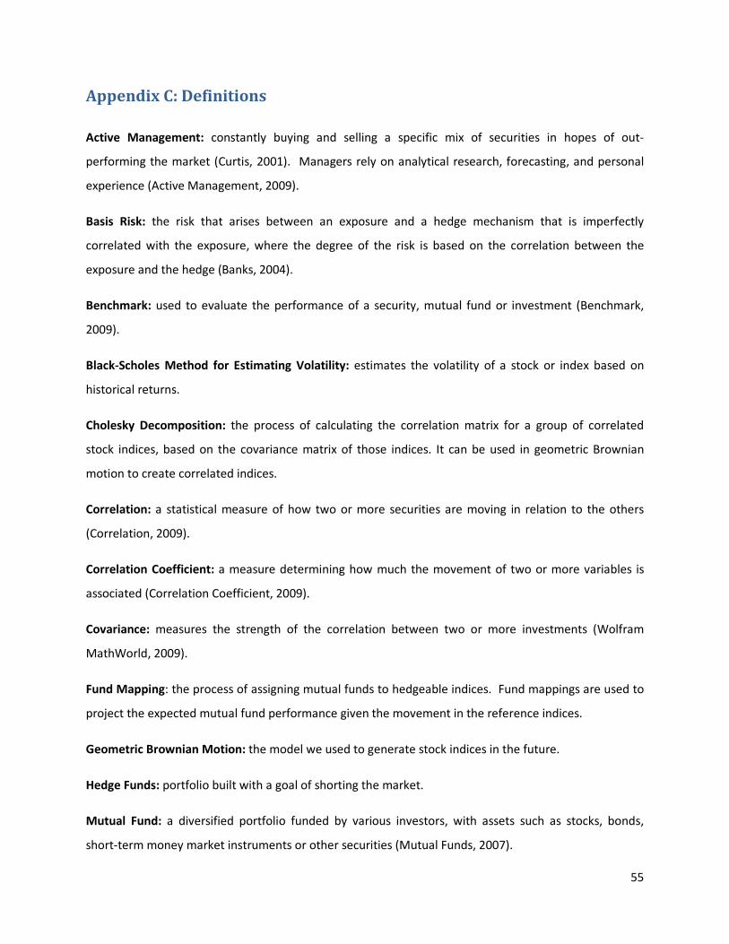
55

Appendix C: Definitions

Active Management: constantly buying and selling a specific mix of securities in hopes of out-

performing the market (Curtis, 2001). Managers rely on analytical research, forecasting, and personal

experience (Active Management, 2009).

Basis Risk: the risk that arises between an exposure and a hedge mechanism that is imperfectly

correlated with the exposure, where the degree of the risk is based on the correlation between the

exposure and the hedge (Banks, 2004).

Benchmark: used to evaluate the performance of a security, mutual fund or investment (Benchmark,

2009).

Black-Scholes Method for Estimating Volatility: estimates the volatility of a stock or index based on

historical returns.

Cholesky Decomposition: the process of calculating the correlation matrix for a group of correlated

stock indices, based on the covariance matrix of those indices. It can be used in geometric Brownian

motion to create correlated indices.

Correlation: a statistical measure of how two or more securities are moving in relation to the others

(Correlation, 2009).

Correlation Coefficient: a measure determining how much the movement of two or more variables is

associated (Correlation Coefficient, 2009).

Covariance: measures the strength of the correlation between two or more investments (Wolfram

MathWorld, 2009).

Fund Mapping: the process of assigning mutual funds to hedgeable indices. Fund mappings are used to

project the expected mutual fund performance given the movement in the reference indices.

Geometric Brownian Motion: the model we used to generate stock indices in the future.

Hedge Funds: portfolio built with a goal of shorting the market.

Mutual Fund: a diversified portfolio funded by various investors, with assets such as stocks, bonds,

short-term money market instruments or other securities (Mutual Funds, 2007).

56

Multicollinearity: a statistical anomaly that occurs when two or more variables in a multiple regression

are highly correlated.

Regression: a measure that is used to determine the strength of a relationship between one dependent

variable and one or more independent variables (Regression, 2009).

Shorting the Market: a portfolio is shorting the market when the value of the portfolio is increasing

while the market is declining.

Tracking Error: the difference between the price behavior of a portfolio and a benchmark (Tracking

Error, 2009).

Variable Annuity: an insurance contract that goes through an accumulation phase and then a payout

phase.

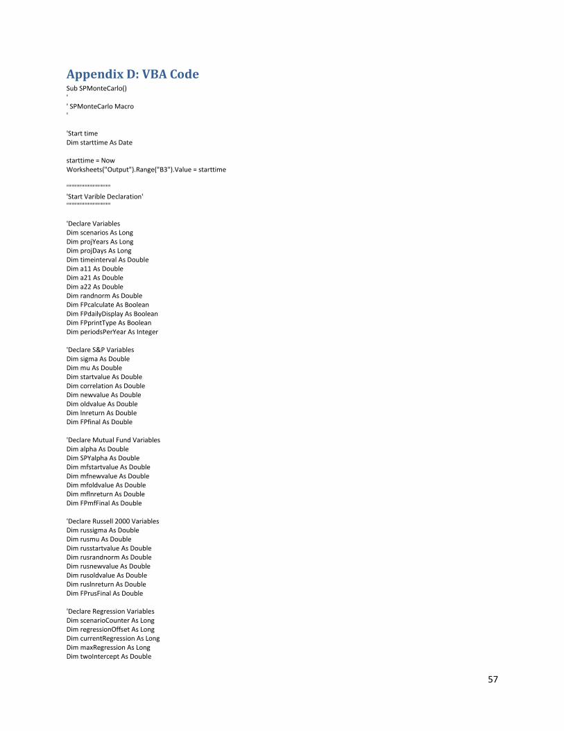
57

Appendix D: VBA Code Sub SPMonteCarlo() ' ' SPMonteCarlo Macro ' 'Start time Dim starttime As Date starttime = Now Worksheets("Output").Range("B3").Value = starttime ''''''''''''''''''''''''''' 'Start Varible Declaration' ''''''''''''''''''''''''''' 'Declare Variables Dim scenarios As Long Dim projYears As Long Dim projDays As Long Dim timeinterval As Double Dim a11 As Double Dim a21 As Double Dim a22 As Double Dim randnorm As Double Dim FPcalculate As Boolean Dim FPdailyDisplay As Boolean Dim FPprintType As Boolean Dim periodsPerYear As Integer 'Declare S&P Variables Dim sigma As Double Dim mu As Double Dim startvalue As Double Dim correlation As Double Dim newvalue As Double Dim oldvalue As Double Dim lnreturn As Double Dim FPfinal As Double 'Declare Mutual Fund Variables Dim alpha As Double Dim SPYalpha As Double Dim mfstartvalue As Double Dim mfnewvalue As Double Dim mfoldvalue As Double Dim mflnreturn As Double Dim FPmfFinal As Double 'Declare Russell 2000 Variables Dim russigma As Double Dim rusmu As Double Dim russtartvalue As Double Dim rusrandnorm As Double Dim rusnewvalue As Double Dim rusoldvalue As Double Dim ruslnreturn As Double Dim FPrusFinal As Double 'Declare Regression Variables Dim scenarioCounter As Long Dim regressionOffset As Long Dim currentRegression As Long Dim maxRegression As Long Dim twoIntercept As Double

58

Dim SP2VarCoeff As Double Dim RUS2VarCoeff As Double Dim SPintercept As Double Dim SP1VarCoeff As Double Dim RUSintercept As Double Dim RUS1VarCoeff As Double Dim regressDaily As Boolean Dim regressLN As Boolean Dim yValues() As Double Dim xValues() As Double Dim x1values() As Double Dim x2values() As Double 'Declare Future Future Variables Dim FFtimeinterval As Double Dim FFmfiB As Double Dim FFmfiBnewvalue As Double Dim FFmfiBoldvalue As Double Dim FFmfiBlnreturn As Double Dim FFmfiC As Double Dim FFmfiClnreturn As Double Dim FFmfiCnewvalue As Double Dim FFmfiColdvalue As Double Dim FFmfiD As Double Dim FFmfiDlnreturn As Double Dim FFmfiDnewvalue As Double Dim FFmfiDoldvalue As Double Dim FFprojYears As Long Dim FFprojDays As Long Dim FFscenarios As Long Dim FFrowOutput As Long Dim FFheaderOutput As Long Dim FFcalculate As Boolean Dim FFdailyDisplay As Boolean Dim FFprintType As Boolean Dim FFperiodsPerYear As Integer 'Set Starting Values for Variables scenarios = Worksheets("Input").Range("B4").Value scenarioCounter = 0 sigma = Worksheets("Input").Range("B8").Value mu = Worksheets("Input").Range("C8").Value correlation = Worksheets("Input").Range("E8").Value projYears = Worksheets("Input").Range("C4").Value projDays = projYears * 252 startvalue = Worksheets("Input").Range("D8").Value timeinterval = Worksheets("Input").Range("G4").Value alpha = Worksheets("Input").Range("B12").Value SPYalpha = Worksheets("Input").Range("C12").Value mfstartvalue = Worksheets("Input").Range("D12").Value russtartvalue = Worksheets("Input").Range("D16").Value rusmu = Worksheets("Input").Range("C16").Value russigma = Worksheets("Input").Range("B16").Value a11 = Worksheets("Input").Range("B19").Value a21 = Worksheets("Input").Range("B20").Value a22 = Worksheets("Input").Range("C20").Value maxRegression = WorksheetFunction.Min(projYears, Worksheets("Input").Range("B24").Value) Worksheets("Input").Range("B24").Value = maxRegression currentRegression = maxRegression FFtimeinterval = Worksheets("Input").Range("G28").Value FFprojYears = Worksheets("Input").Range("C28").Value FFprojDays = FFprojYears * 252 FFscenarios = Worksheets("Input").Range("B28").Value 'Sets Future Past Calculate variable If Worksheets("Input").Range("D4").Value = "Daily" Then

59

'Daily calculation of returns means True FPcalculate = True Else If Worksheets("Input").Range("D4").Value = "Monthly" Then 'Monthly calculation of returns means False FPcalculate = False Else 'When Neither 'Daily' or 'Monthly' is entered, assume 'Daily' Worksheets("Input").Range("D4").Value = "Daily" FPcalculate = True End If End If 'Sets Future Past Display variable If Worksheets("Input").Range("E4").Value = "Daily" Then 'Daily display of data means True FPdailyDisplay = True periodsPerYear = 252 Else If Worksheets("Input").Range("E4").Value = "Monthly" Then 'Monthly display of data means False FPdailyDisplay = False periodsPerYear = 12 Else 'When Neither 'Daily' or 'Monthly' is entered, assume 'Daily' Worksheets("Input").Range("E4").Value = "Daily" FPdailyDisplay = True periodsPerYear = 252 End If End If 'Test If FPcalculate = False Then If FPdailyDisplay = True Then 'Scenarios can't be run with monthly calculations but outputting values daily 'So, switch to monthly output. Worksheets("Input").Range("E4").Value = "Monthly" FPdailyDisplay = False periodsPerYear = 12 End If End If 'If Future Past Display is false (data is shown monthly), then projDays is actually projMonths If FPdailyDisplay = False Then projDays = projYears * 12 End If 'Sets Future Past Print variable If Worksheets("Input").Range("F4").Value = "LN Return" Then 'LN Return output means True FPprintType = True Else If Worksheets("Input").Range("F4").Value = "Values" Then 'Values output means False FPprintType = False Else 'When Neither 'LN Return' or 'Values' is entered, assume 'LN Return' Worksheets("Input").Range("F4").Value = "LN Return" FPprintType = True End If End If 'Sets Regression Calculating Variable If Worksheets("Input").Range("C24").Value = "Daily" Then 'Regressing daily means True regressDaily = True

60

Else If Worksheets("Input").Range("C24").Value = "Monthly" Then 'Regressing monthly means False regressDaily = False Else 'When Neither 'Daily' or 'Monthly is entered, assume 'Daily' Worksheets("Input").Range("C24").Value = "Daily" regressDaily = True End If End If 'Test If FPdailyDisplay = False Then If regressDaily = True Then 'Regressions can't be done daily if there is only monthly data for the scenarios 'So, switch to monthly regression. Worksheets("Input").Range("C24").Value = "Monthly" regressDaily = False End If End If 'Sets whether to regress the ln returns or index values If Worksheets("Input").Range("D24").Value = "LN Return" Then 'LN Regression means true regressLN = True Else If Worksheets("Input").Range("D24").Value = "Values" Then 'Values Regression means false regressLN = False Else 'When Neither 'LN Return' or 'Values' is entered, assume 'LN Return' Worksheets("Input").Range("D24").Value = "LN Return" regressLN = True End If End If 'Sets Future Future Calculate variable If Worksheets("Input").Range("D28").Value = "Daily" Then 'Daily calculation of returns means True FFcalculate = True Else If Worksheets("Input").Range("D28").Value = "Monthly" Then 'Monthly calculation of returns means False FFcalculate = False Else 'When Neither 'Daily' or 'Monthly' is entered, assume 'Daily' Worksheets("Input").Range("D28").Value = "Daily" FFcalculate = True End If End If 'Sets Future Future Display variable If Worksheets("Input").Range("E28").Value = "Daily" Then 'Daily display of data means True FFdailyDisplay = True FFperiodsPerYear = 252 Else If Worksheets("Input").Range("E28").Value = "Monthly" Then 'Monthly display of data means False FFdailyDisplay = False FFperiodsPerYear = 12 Else 'When Neither 'Daily' or 'Monthly' is entered, assume 'Daily' Worksheets("Input").Range("E28").Value = "Daily" FFdailyDisplay = True FFperiodsPerYear = 252

61

End If End If 'Test If FFcalculate = False Then If FFdailyDisplay = True Then 'Scenarios can't be run with monthly calculations but outputting values daily 'So, switch to monthly output. Worksheets("Input").Range("E28").Value = "Monthly" FFdailyDisplay = False FFperiodsPerYear = 12 End If End If 'If Future Future Display is false (data is shown monthly), then FFprojDays is actually FFprojMonths If FFdailyDisplay = False Then FFprojDays = FFprojYears * 12 End If 'Sets Future Future Print variable If Worksheets("Input").Range("F28").Value = "LN Return" Then 'LN Return output means True FFprintType = True Else If Worksheets("Input").Range("F28").Value = "Values" Then 'Values output means False FFprintType = False Else 'When Neither 'LN Return' or 'Values' is entered, assume 'LN Return' Worksheets("Input").Range("F28").Value = "LN Return" FFprintType = True End If End If ''''''''''''''''''''''''' 'End Varible Declaration' ''''''''''''''''''''''''' 'Backup old "Scenario Output" Worksheet Dim oldoutputs As Integer Dim sheet As Integer sheet = 1 Do While sheet < Worksheets.Count + Charts.Count + 1 If Sheets(sheet).Name = "Scenario Output" Then oldoutputs = 1 sheet = 1 Do While sheet < Worksheets.Count + Charts.Count + 1 If Sheets(sheet).Name = "Scenario Output Old" & oldoutputs Then oldoutputs = oldoutputs + 1 sheet = 0 End If sheet = sheet + 1 Loop Worksheets("Scenario Output").Name = "Scenario Output Old" & oldoutputs End If sheet = sheet + 1 Loop 'New "Scenario Outputs" Worksheet Sheets.Add Before:=Worksheets("Output") ActiveSheet.Name = "Scenario Output" ActiveWindow.Zoom = 85 '''''''''''''''''''''''''' 'Formatting New Worksheet'

62

'''''''''''''''''''''''''' 'Status Update Worksheets("Scenario Output").Range("A1").Font.Size = 10 Worksheets("Scenario Output").Range("A1").Value = "Initializing..." 'Column Height Worksheets("Scenario Output").Columns.ColumnWidth = 8.57 Worksheets("Scenario Output").Columns(1).ColumnWidth = 13.51 'Number Formatting Worksheets("Scenario Output").Columns.NumberFormat = "0.0000" If FPprintType = True Then For i = 1 To projDays + 2 'If printing LN Returns, use percentage Worksheets("Scenario Output").Rows(i).NumberFormat = "0.00%" Next i Else For i = 1 To projDays + 2 'If printing values, use number Worksheets("Scenario Output").Rows(i).NumberFormat = "0.00" Next i End If If FFprintType = False Then 'If printing values, use number For i = 1 To FFscenarios * (maxRegression + 1) For j = 1 To FFprojDays Worksheets("Scenario Output").Rows(7 + j + 25 * maxRegression + projDays + (i - 1) * (FFprojDays + 2)).NumberFormat = "0.00" Next j Next i Else 'If printing LN Returns, use value For i = 1 To FFscenarios * (maxRegression + 1) For j = 1 To FFprojDays Worksheets("Scenario Output").Rows(7 + j + 25 * maxRegression + projDays + (i - 1) * (FFprojDays + 2)).NumberFormat = "0.00%" Next j Next i End If Worksheets("Scenario Output").Columns(1).NumberFormat = "0" 'Status Update Worksheets("Scenario Output").Range("A1").Value = "Formatting..." 'Bolding Stuff Worksheets("Scenario Output").Columns(1).Font.FontStyle = "Bold" Worksheets("Scenario Output").Rows("1:2").Font.FontStyle = "Bold" Worksheets("Scenario Output").Range("A1").Font.FontStyle = "Unbold" For i = 1 To FFscenarios * (maxRegression + 1) Worksheets("Scenario Output").Rows(6 + 25 * maxRegression + projDays + (i - 1) * (FFprojDays + 2)).Font.FontStyle = "Bold" Worksheets("Scenario Output").Rows(7 + 25 * maxRegression + projDays + (i - 1) * (FFprojDays + 2)).Font.FontStyle = "Bold" Next i 'Enlarging Fonts Worksheets("Scenario Output").Rows("1:2").Font.Size = 14 Worksheets("Scenario Output").Range("A1").Font.Size = 10 For i = 1 To FFscenarios * (maxRegression + 1) Worksheets("Scenario Output").Rows(6 + 25 * maxRegression + projDays + (i - 1) * (FFprojDays + 2)).Font.Size = 14 Worksheets("Scenario Output").Rows(7 + 25 * maxRegression + projDays + (i - 1) * (FFprojDays + 2)).Font.Size = 14 Next i 'Borders With Worksheets("Scenario Output").Rows(2).Borders(xlEdgeBottom) .LineStyle = xlContinuous .ColorIndex = xlAutomatic .TintAndShade = 0 .Weight = xlThin

63

End With With Worksheets("Scenario Output").Rows(3).Borders(xlEdgeTop) .LineStyle = xlContinuous .ColorIndex = xlAutomatic .TintAndShade = 0 .Weight = xlThin End With With Worksheets("Scenario Output").Columns(1).Borders(xlEdgeRight) .LineStyle = xlContinuous .ColorIndex = xlAutomatic .TintAndShade = 0 .Weight = xlThin End With With Worksheets("Scenario Output").Columns(2).Borders(xlEdgeLeft) .LineStyle = xlContinuous .ColorIndex = xlAutomatic .TintAndShade = 0 .Weight = xlThin End With For i = 1 To FFscenarios * (maxRegression + 1) With Worksheets("Scenario Output").Rows(5 + 25 * maxRegression + projDays + (i - 1) * (FFprojDays + 2)).Borders(xlEdgeBottom) .LineStyle = xlContinuous .ColorIndex = xlAutomatic .TintAndShade = 0 .Weight = xlThick End With With Worksheets("Scenario Output").Rows(6 + 25 * maxRegression + projDays + (i - 1) * (FFprojDays + 2)).Borders(xlEdgeTop) .LineStyle = xlContinuous .ColorIndex = xlAutomatic .TintAndShade = 0 .Weight = xlThick End With With Worksheets("Scenario Output").Rows(7 + 25 * maxRegression + projDays + (i - 1) * (FFprojDays + 2)).Borders(xlEdgeBottom) .LineStyle = xlContinuous .ColorIndex = xlAutomatic .TintAndShade = 0 .Weight = xlThin End With With Worksheets("Scenario Output").Rows(8 + 25 * maxRegression + projDays + (i - 1) * (FFprojDays + 2)).Borders(xlEdgeTop) .LineStyle = xlContinuous .ColorIndex = xlAutomatic .TintAndShade = 0 .Weight = xlThin End With Next i With Worksheets("Scenario Output").Rows(5 + 25 * maxRegression + projDays + FFscenarios * (maxRegression + 1) * (FFprojDays + 2)).Borders(xlEdgeBottom) .LineStyle = xlContinuous .ColorIndex = xlAutomatic .TintAndShade = 0 .Weight = xlThick End With With Worksheets("Scenario Output").Rows(6 + 25 * maxRegression + projDays + FFscenarios * (maxRegression + 1) * (FFprojDays + 2)).Borders(xlEdgeTop) .LineStyle = xlContinuous .ColorIndex = xlAutomatic .TintAndShade = 0 .Weight = xlThick End With With Worksheets("Scenario Output").Rows(5 + 25 * maxRegression + projDays + FFscenarios * maxRegression * (FFprojDays + 2)).Borders(xlEdgeBottom) .LineStyle = xlContinuous .ColorIndex = xlAutomatic .TintAndShade = 0 .Weight = xlThick End With

64

With Worksheets("Scenario Output").Rows(6 + 25 * maxRegression + projDays + FFscenarios * maxRegression * (FFprojDays + 2)).Borders(xlEdgeTop) .LineStyle = xlContinuous .ColorIndex = xlAutomatic .TintAndShade = 0 .Weight = xlThick End With 'Display Period Numbers If FPdailyDisplay = False Then If FPcalculate = True Then If FPprintType = True Then 'For Monthly periods with daily LN Return calculations Worksheets("Scenario Output").Range("A2").Value = "Months (LN Returns, calculated Daily)" Else 'For Monthly periods with monthly Value calculations Worksheets("Scenario Output").Range("A2").Value = "Months (Index Values, calculated Daily)" End If Else If FPprintType = True Then 'For Monthly periods with monthly LN Return calculations Worksheets("Scenario Output").Range("A2").Value = "Months (LN Returns, calculated Monthly)" Else 'For Monthly periods with monthly Value calculations Worksheets("Scenario Output").Range("A2").Value = "Months (Index Values, calculated Monthly)" End If End If Else If FPprintType = True Then 'For Daily periods with daily LN Return calculations Worksheets("Scenario Output").Range("A2").Value = "Days (LN Returns, calculated Daily)" Else 'For Daily periods with daily Value calculations Worksheets("Scenario Output").Range("A2").Value = "Days (Index Values, calculated Daily)" End If End If For i = 1 To projDays Worksheets("Scenario Output").Cells(i + 2, 1).Value = i Next i 'Print Regression Years on Left Side If regressLN = True Then If regressDaily = True Then Worksheets("Scenario Output").Cells(projDays + 4, 1).Value = "Regressions (LN Returns, calculated Daily)" Else Worksheets("Scenario Output").Cells(projDays + 4, 1).Value = "Regressions (LN Returns, calculated Monthly)" End If Else If regressDaily = True Then Worksheets("Scenario Output").Cells(projDays + 4, 1).Value = "Regressions (Index Values, calculated Daily)" Else Worksheets("Scenario Output").Cells(projDays + 4, 1).Value = "Regressions (Index Values, calculated Monthly)" End If End If Worksheets("Scenario Output").Cells(projDays + 4, 1).Font.Size = 14 Do While currentRegression > 0 Worksheets("Scenario Output").Cells((maxRegression - currentRegression) * 25 + projDays + 5, 1).Value = currentRegression & " YEAR" currentRegression = currentRegression - 1 Loop currentRegression = maxRegression '''''''''''''''''''''''''''' 'Formatting Stuff Ends Here' '''''''''''''''''''''''''''' ''''''''''''''''''''''''''''

65

'Scenario Stuff Starts Here' '''''''''''''''''''''''''''' 'Start Scenario Loop Do While scenarioCounter < scenarios 'Randomize Randomize 'Status Update Worksheets("Scenario Output").Range("A1").Value = "Calculating Scenario " & scenarioCounter + 1 & "..." 'Output Scenario Heading Worksheets("Scenario Output").Cells(1, scenarioCounter * 4 + 2).Value = "Scenario " & scenarioCounter + 1 Worksheets("Scenario Output").Cells(2, scenarioCounter * 4 + 2).Value = "MFI" Worksheets("Scenario Output").Cells(2, scenarioCounter * 4 + 3).Value = "SPY" Worksheets("Scenario Output").Cells(2, scenarioCounter * 4 + 4).Value = "RUS" 'Reset Variables startvalue = Worksheets("Input").Range("D8").Value mfstartvalue = Worksheets("Input").Range("D12").Value russtartvalue = Worksheets("Input").Range("D16").Value newvalue = startvalue rusnewvalue = russtartvalue mfnewvalue = mfstartvalue ''''''''''''''''''''''''''''''' 'Future Past Stuff Starts Here' ''''''''''''''''''''''''''''''' 'Start Daily Projection Loop for Future Past For currentday = 0 To projDays - 1 'Previous New Values become Old Values oldvalue = newvalue rusoldvalue = rusnewvalue mfoldvalue = mfnewvalue 'This top part of the If statement is used when the indexes are calcuated at the same times they are outputted If (FPdailyDisplay = True And FPcalculate = True) Or (FPdailyDisplay = False And FPcalculate = False) Then 'Reset Random Numbers randnorm = Application.WorksheetFunction.NormSInv(Rnd()) rusrandnorm = Application.WorksheetFunction.NormSInv(Rnd()) mfrandnorm = Application.WorksheetFunction.NormSInv(Rnd()) 'Calculate New Values newvalue = newvalue * Exp((mu - variance ^ 2 / 2) * timeinterval + timeinterval ^ 0.5 * a11 * randnorm) rusnewvalue = rusnewvalue * Exp((rusmu - rusvariance ^ 2 / 2) * timeinterval + timeinterval ^ 0.5 * (a21 * randnorm + a22 * rusrandnorm)) 'Calculate ln of Returns lnreturn = Log(newvalue / oldvalue) ruslnreturn = Log(rusnewvalue / rusoldvalue) mflnreturn = lnreturn + (alpha + Abs(SPYalpha * lnreturn)) / (periodsPerYear ^ 0.5) * mfrandnorm 'Calculate New value of Mutual Fund mfnewvalue = Exp(mflnreturn) * mfoldvalue Else 'This portion is used when the indexes are calcuated daily, but values are outputted monthly For i = 1 To 21 'Reset Random Numbers randnorm = Application.WorksheetFunction.NormSInv(Rnd()) rusrandnorm = Application.WorksheetFunction.NormSInv(Rnd()) mfrandnorm = Application.WorksheetFunction.NormSInv(Rnd())

66

'Calculate New Values newvalue = newvalue * Exp((mu - variance ^ 2 / 2) * timeinterval + timeinterval ^ 0.5 * a11 * randnorm) rusnewvalue = rusnewvalue * Exp((rusmu - rusvariance ^ 2 / 2) * timeinterval + timeinterval ^ 0.5 * (a21 * randnorm + a22 * rusrandnorm)) mfnewvalue = mfnewvalue * Exp((mu - variance ^ 2 / 2) * timeinterval + timeinterval ^ 0.5 * a11 * randnorm + (alpha + Abs(SPYalpha * ((mu - variance ^ 2 / 2) * timeinterval + timeinterval ^ 0.5 * a11 * randnorm))) / (252 ^ 0.5) * mfrandnorm) Next i 'Calculate ln of Returns lnreturn = Log(newvalue / oldvalue) ruslnreturn = Log(rusnewvalue / rusoldvalue) mflnreturn = Log(mfnewvalue / mfoldvalue) End If If FPprintType = True Then 'Output ln of Returns Worksheets("Scenario Output").Cells(currentday + 3, scenarioCounter * 4 + 2).Value = mflnreturn Worksheets("Scenario Output").Cells(currentday + 3, scenarioCounter * 4 + 3).Value = lnreturn Worksheets("Scenario Output").Cells(currentday + 3, scenarioCounter * 4 + 4).Value = ruslnreturn Else 'Output Index Values Worksheets("Scenario Output").Cells(currentday + 3, scenarioCounter * 4 + 2).Value = mfnewvalue Worksheets("Scenario Output").Cells(currentday + 3, scenarioCounter * 4 + 3).Value = newvalue Worksheets("Scenario Output").Cells(currentday + 3, scenarioCounter * 4 + 4).Value = rusnewvalue End If Next currentday 'Preserve Final Values FPfinal = newvalue FPrusFinal = rusnewvalue FPmfFinal = mfnewvalue 'Print Borders With Worksheets("Scenario Output").Columns(scenarioCounter * 4 + 5).Borders(xlEdgeRight) .LineStyle = xlContinuous .ColorIndex = xlAutomatic .TintAndShade = 0 .Weight = xlThin End With With Worksheets("Scenario Output").Columns(scenarioCounter * 4 + 2).Borders(xlEdgeLeft) .LineStyle = xlContinuous .ColorIndex = xlAutomatic .TintAndShade = 0 .Weight = xlThin End With 'Color Columns With Worksheets("Scenario Output").Range(Cells(1, scenarioCounter * 4 + 2), Cells(projDays + 2, scenarioCounter * 4 + 2)).Interior .Pattern = xlSolid .PatternColorIndex = xlAutomatic .Color = 5296274 .TintAndShade = 0 .PatternTintAndShade = 0 End With With Worksheets("Scenario Output").Range(Cells(1, scenarioCounter * 4 + 3), Cells(projDays + 2, scenarioCounter * 4 + 3)).Interior .Pattern = xlSolid .PatternColorIndex = xlAutomatic .Color = 14136213 .TintAndShade = 0 .PatternTintAndShade = 0 End With With Worksheets("Scenario Output").Range(Cells(1, scenarioCounter * 4 + 4), Cells(projDays + 2, scenarioCounter * 4 + 4)).Interior .Pattern = xlSolid .PatternColorIndex = xlAutomatic .Color = 49407

67

.TintAndShade = 0 .PatternTintAndShade = 0 End With 'Merge Top Row With Worksheets("Scenario Output").Range(Cells(1, scenarioCounter * 4 + 2), Cells(1, scenarioCounter * 4 + 4)) .Merge .HorizontalAlignment = xlCenter .VerticalAlignment = xlBottom .Interior.Color = 8421631 End With ''''''''''''''''''''''''''''' 'Future Past Stuff Ends Here' ''''''''''''''''''''''''''''' '''''''''''''''''''''''''''''' 'Regression Stuff Starts Here' '''''''''''''''''''''''''''''' 'Status Update Worksheets("Scenario Output").Range("A1").Value = "Regressing Scenario " & scenarioCounter + 1 & "..." currentRegression = maxRegression Do While currentRegression > 0 regressionOffset = (maxRegression - currentRegression) * 25 + projDays ''''''''''''''''''''''''''''' 'POPULATING ARRAYS WITH DATA' ''''''''''''''''''''''''''''' 'This top part of the If statement is used when the regression is performed on all outputted values If (FPdailyDisplay = True And regressDaily = True) Or (FPdailyDisplay = False And regressDaily = False) Then ReDim yValues(1 To projDays - (maxRegression - currentRegression) * periodsPerYear) As Double ReDim x1values(1 To projDays - (maxRegression - currentRegression) * periodsPerYear) As Double ReDim x2values(1 To projDays - (maxRegression - currentRegression) * periodsPerYear) As Double ReDim xValues(1 To 2, 1 To projDays - (maxRegression - currentRegression) * periodsPerYear) As Double 'Checks if the scenarios are outputted in the same way (ln or values) that the regression will be done If (FPprintType = True And regressLN = True) Or (FPprintType = False And regressLN = False) Then 'Populate the Arrays with the correct values For i = 1 To projDays - (projYears - currentRegression) * periodsPerYear yValues(i) = Worksheets("Scenario Output").Cells((projYears - currentRegression) * periodsPerYear + i + 2, scenarioCounter * 4 + 2).Value x1values(i) = Worksheets("Scenario Output").Cells((projYears - currentRegression) * periodsPerYear + i + 2, scenarioCounter * 4 + 3).Value x2values(i) = Worksheets("Scenario Output").Cells((projYears - currentRegression) * periodsPerYear + i + 2, scenarioCounter * 4 + 4).Value xValues(1, i) = x1values(i) xValues(2, i) = x2values(i) Next i Else 'This is used if the scenarios are outputted as values, but the regression will be done on ln If regressLN = True And FPprintType = False Then 'Populate the Arrays with the correct values If currentRegression = projYears Then yValues(1) = Log(Worksheets("Scenario Output").Cells(3, scenarioCounter * 4 + 2).Value / mfstartvalue) x1values(1) = Log(Worksheets("Scenario Output").Cells(3, scenarioCounter * 4 + 3).Value / startvalue) x2values(1) = Log(Worksheets("Scenario Output").Cells(3, scenarioCounter * 4 + 4).Value / russtartvalue) Else

68

yValues(1) = Log(Worksheets("Scenario Output").Cells((projYears - currentRegression) * periodsPerYear + 3, scenarioCounter * 4 + 2).Value / Worksheets("Scenario Output").Cells((projYears - currentRegression) * periodsPerYear + 2, scenarioCounter * 4 + 2).Value) x1values(1) = Log(Worksheets("Scenario Output").Cells((projYears - currentRegression) * periodsPerYear + 3, scenarioCounter * 4 + 3).Value / Worksheets("Scenario Output").Cells((projYears - currentRegression) * periodsPerYear + 2, scenarioCounter * 4 + 3).Value) x2values(1) = Log(Worksheets("Scenario Output").Cells((projYears - currentRegression) * periodsPerYear + 3, scenarioCounter * 4 + 4).Value / Worksheets("Scenario Output").Cells((projYears - currentRegression) * periodsPerYear + 2, scenarioCounter * 4 + 4).Value) End If xValues(1, 1) = x1values(1) xValues(2, 1) = x2values(1) For i = 2 To projDays - (projYears - currentRegression) * periodsPerYear yValues(i) = Log(Worksheets("Scenario Output").Cells((projYears - currentRegression) * periodsPerYear + i + 2, scenarioCounter * 4 + 2).Value / Worksheets("Scenario Output").Cells((projYears - currentRegression) * periodsPerYear + i + 1, scenarioCounter * 4 + 2).Value) x1values(i) = Log(Worksheets("Scenario Output").Cells((projYears - currentRegression) * periodsPerYear + i + 2, scenarioCounter * 4 + 3).Value / Worksheets("Scenario Output").Cells((projYears - currentRegression) * periodsPerYear + i + 1, scenarioCounter * 4 + 3).Value) x2values(i) = Log(Worksheets("Scenario Output").Cells((projYears - currentRegression) * periodsPerYear + i + 2, scenarioCounter * 4 + 4).Value / Worksheets("Scenario Output").Cells((projYears - currentRegression) * periodsPerYear + i + 1, scenarioCounter * 4 + 4).Value) xValues(1, i) = x1values(i) xValues(2, i) = x2values(i) Next i Else 'This is used if the scenarios are outputted as ln, but the regression will be done on values 'Populate the Arrays with the correct values If currentRegression = projYears Then yValues(1) = mfstartvalue * Exp(Worksheets("Scenario Output").Cells(3, scenarioCounter * 4 + 2).Value) x1values(1) = startvalue * Exp(Worksheets("Scenario Output").Cells(3, scenarioCounter * 4 + 3).Value) x2values(1) = russtartvalue * Exp(Worksheets("Scenario Output").Cells(3, scenarioCounter * 4 + 4).Value) Else yValues(1) = mfstartvalue * Exp(Application.WorksheetFunction.Sum(Worksheets("Scenario Output").Range(Cells(3, scenarioCounter * 4 + 2), Cells((projYears - currentRegression) * periodsPerYear + 3, scenarioCounter * 4 + 2)).Value)) x1values(1) = startvalue * Exp(Application.WorksheetFunction.Sum(Worksheets("Scenario Output").Range(Cells(3, scenarioCounter * 4 + 3), Cells((projYears - currentRegression) * periodsPerYear + 3, scenarioCounter * 4 + 3)).Value)) x2values(1) = russtartvalue * Exp(Application.WorksheetFunction.Sum(Worksheets("Scenario Output").Range(Cells(3, scenarioCounter * 4 + 4), Cells((projYears - currentRegression) * periodsPerYear + 3, scenarioCounter * 4 + 4)).Value)) End If xValues(1, 1) = x1values(1) xValues(2, 1) = x2values(1) For i = 2 To projDays - (projYears - currentRegression) * periodsPerYear yValues(i) = yValues(i - 1) * Exp(Worksheets("Scenario Output").Cells((projYears - currentRegression) * periodsPerYear + 2 + i, scenarioCounter * 4 + 2).Value) x1values(i) = x1values(i - 1) * Exp(Worksheets("Scenario Output").Cells((projYears - currentRegression) * periodsPerYear + 2 + i, scenarioCounter * 4 + 3).Value) x2values(i) = x2values(i - 1) * Exp(Worksheets("Scenario Output").Cells((projYears - currentRegression) * periodsPerYear + 2 + i, scenarioCounter * 4 + 4).Value) xValues(1, i) = x1values(i) xValues(2, i) = x2values(i) Next i End If End If 'This portion is used when the indexes are outputted daily, but regression is done monthly Else ReDim yValues(1 To (projDays - (maxRegression - currentRegression) * periodsPerYear) / 21) As Double ReDim x1values(1 To (projDays - (maxRegression - currentRegression) * periodsPerYear) / 21) As Double ReDim x2values(1 To (projDays - (maxRegression - currentRegression) * periodsPerYear) / 21) As Double ReDim xValues(1 To 2, 1 To (projDays - (maxRegression - currentRegression) * periodsPerYear) / 21) As Double 'Checks if the scenarios are outputted in the same way (ln or values) that the regression will be done

69

If (FPprintType = True And regressLN = True) Or (FPprintType = False And regressLN = False) Then 'Populate the Arrays with the correct values (i*21 because 21 trading days per month) For i = 1 To (projDays - (projYears - currentRegression) * periodsPerYear) / 21 yValues(i) = Worksheets("Scenario Output").Cells((projYears - currentRegression) * periodsPerYear + i * 21 + 2, scenarioCounter * 4 + 2).Value x1values(i) = Worksheets("Scenario Output").Cells((projYears - currentRegression) * periodsPerYear + i * 21 + 2, scenarioCounter * 4 + 3).Value x2values(i) = Worksheets("Scenario Output").Cells((projYears - currentRegression) * periodsPerYear + i * 21 + 2, scenarioCounter * 4 + 4).Value xValues(1, i) = x1values(i) xValues(2, i) = x2values(i) Next i Else 'This is used if the scenarios are outputted as values, but the regression will be done on ln If regressLN = True And FPprintType = False Then 'Populate the Arrays with the correct values If currentRegression = projYears Then yValues(1) = Log(Worksheets("Scenario Output").Cells(23, scenarioCounter * 4 + 2).Value / mfstartvalue) x1values(1) = Log(Worksheets("Scenario Output").Cells(23, scenarioCounter * 4 + 3).Value / startvalue) x2values(1) = Log(Worksheets("Scenario Output").Cells(23, scenarioCounter * 4 + 4).Value / russtartvalue) Else yValues(1) = Log(Worksheets("Scenario Output").Cells((projYears - currentRegression) * periodsPerYear + 23, scenarioCounter * 4 + 2).Value / Worksheets("Scenario Output").Cells((projYears - currentRegression) * periodsPerYear + 2, scenarioCounter * 4 + 2).Value) x1values(1) = Log(Worksheets("Scenario Output").Cells((projYears - currentRegression) * periodsPerYear + 23, scenarioCounter * 4 + 3).Value / Worksheets("Scenario Output").Cells((projYears - currentRegression) * periodsPerYear + 2, scenarioCounter * 4 + 3).Value) x2values(1) = Log(Worksheets("Scenario Output").Cells((projYears - currentRegression) * periodsPerYear + 23, scenarioCounter * 4 + 4).Value / Worksheets("Scenario Output").Cells((projYears - currentRegression) * periodsPerYear + 2, scenarioCounter * 4 + 4).Value) End If xValues(1, 1) = x1values(1) xValues(2, 1) = x2values(1) For i = 2 To (projDays - (projYears - currentRegression) * periodsPerYear) / 21 yValues(i) = Log(Worksheets("Scenario Output").Cells((projYears - currentRegression) * periodsPerYear + i * 21 + 2, scenarioCounter * 4 + 2).Value / Worksheets("Scenario Output").Cells((projYears - currentRegression) * periodsPerYear + (i - 1) * 21 + 2, scenarioCounter * 4 + 2).Value) x1values(i) = Log(Worksheets("Scenario Output").Cells((projYears - currentRegression) * periodsPerYear + i * 21 + 2, scenarioCounter * 4 + 3).Value / Worksheets("Scenario Output").Cells((projYears - currentRegression) * periodsPerYear + (i - 1) * 21 + 2, scenarioCounter * 4 + 3).Value) x2values(i) = Log(Worksheets("Scenario Output").Cells((projYears - currentRegression) * periodsPerYear + i * 21 + 2, scenarioCounter * 4 + 4).Value / Worksheets("Scenario Output").Cells((projYears - currentRegression) * periodsPerYear + (i - 1) * 21 + 2, scenarioCounter * 4 + 4).Value) xValues(1, i) = x1values(i) xValues(2, i) = x2values(i) Next i Else 'This is used if the scenarios are outputted as ln, but the regression will be done on values 'Populate the Arrays with the correct values If currentRegression = projYears Then yValues(1) = mfstartvalue * Exp(Application.WorksheetFunction.Sum(Worksheets("Scenario Output").Range(Cells(3, scenarioCounter * 4 + 2), Cells(23, scenarioCounter * 4 + 2)).Value)) x1values(1) = startvalue * Exp(Application.WorksheetFunction.Sum(Worksheets("Scenario Output").Range(Cells(3, scenarioCounter * 4 + 3), Cells(23, scenarioCounter * 4 + 3)).Value)) x2values(1) = russtartvalue * Exp(Application.WorksheetFunction.Sum(Worksheets("Scenario Output").Range(Cells(3, scenarioCounter * 4 + 4), Cells(23, scenarioCounter * 4 + 4)).Value)) Else yValues(1) = mfstartvalue * Exp(Application.WorksheetFunction.Sum(Worksheets("Scenario Output").Range(Cells(3, scenarioCounter * 4 + 2), Cells((projYears - currentRegression) * periodsPerYear + 23, scenarioCounter * 4 + 2)).Value)) x1values(1) = startvalue * Exp(Application.WorksheetFunction.Sum(Worksheets("Scenario Output").Range(Cells(3, scenarioCounter * 4 + 3), Cells((projYears - currentRegression) * periodsPerYear + 23, scenarioCounter * 4 + 3)).Value))

70

x2values(1) = russtartvalue * Exp(Application.WorksheetFunction.Sum(Worksheets("Scenario Output").Range(Cells(3, scenarioCounter * 4 + 4), Cells((projYears - currentRegression) * periodsPerYear + 23, scenarioCounter * 4 + 4)).Value)) End If xValues(1, 1) = x1values(1) xValues(2, 1) = x2values(1) For i = 2 To (projDays - (projYears - currentRegression) * periodsPerYear) / 21 yValues(i) = yValues(i - 1) * Exp(Application.WorksheetFunction.Sum(Worksheets("Scenario Output").Range(Cells((projYears - currentRegression) * periodsPerYear + 3 + (i - 1) * 21, scenarioCounter * 4 + 2), Cells((projYears - currentRegression) * periodsPerYear + 2 + i * 21, scenarioCounter * 4 + 2)).Value)) x1values(i) = x1values(i - 1) * Exp(Application.WorksheetFunction.Sum(Worksheets("Scenario Output").Range(Cells((projYears - currentRegression) * periodsPerYear + 3 + (i - 1) * 21, scenarioCounter * 4 + 3), Cells((projYears - currentRegression) * periodsPerYear + 2 + i * 21, scenarioCounter * 4 + 3)).Value)) x2values(i) = x2values(i - 1) * Exp(Application.WorksheetFunction.Sum(Worksheets("Scenario Output").Range(Cells((projYears - currentRegression) * periodsPerYear + 3 + (i - 1) * 21, scenarioCounter * 4 + 4), Cells((projYears - currentRegression) * periodsPerYear + 2 + i * 21, scenarioCounter * 4 + 4)).Value)) xValues(1, i) = x1values(i) xValues(2, i) = x2values(i) Next i End If End If End If '''''''''''''''''''''''''''''''''''''''''''''''''''''''''''''' 'POPULATING ARRAYS WITH DATA IS DONE. NOW, REGRESS THE ARRAYS' '''''''''''''''''''''''''''''''''''''''''''''''''''''''''''''' '2 Variable Regression Worksheets("Scenario Output").Range(Cells(regressionOffset + 9, scenarioCounter * 4 + 2), Cells(regressionOffset + 13, scenarioCounter * 4 + 4)).Value = WorksheetFunction.LinEst(yValues, xValues, True, True) 'Formatting for 2 Variable Regression Worksheets("Scenario Output").Cells(regressionOffset + 6, scenarioCounter * 4 + 2).Value = "2-VAR" Worksheets("Scenario Output").Cells(regressionOffset + 7, scenarioCounter * 4 + 2).Value = "SPY" Worksheets("Scenario Output").Cells(regressionOffset + 8, scenarioCounter * 4 + 2).Value = "RUS" twoIntercept = Worksheets("Scenario Output").Cells(regressionOffset + 9, scenarioCounter * 4 + 4).Value SP2VarCoeff = Worksheets("Scenario Output").Cells(regressionOffset + 9, scenarioCounter * 4 + 3).Value RUS2VarCoeff = Worksheets("Scenario Output").Cells(regressionOffset + 9, scenarioCounter * 4 + 2).Value Worksheets("Scenario Output").Cells(regressionOffset + 6, scenarioCounter * 4 + 3).Value = twoIntercept Worksheets("Scenario Output").Cells(regressionOffset + 7, scenarioCounter * 4 + 3).Value = SP2VarCoeff Worksheets("Scenario Output").Cells(regressionOffset + 8, scenarioCounter * 4 + 3).Value = RUS2VarCoeff Worksheets("Scenario Output").Range(Cells(regressionOffset + 6, scenarioCounter * 4 + 2), Cells(regressionOffset + 8, scenarioCounter * 4 + 3)).Font.FontStyle = "Bold" Worksheets("Scenario Output").Range(Cells(regressionOffset + 11, scenarioCounter * 4 + 4), Cells(regressionOffset + 13, scenarioCounter * 4 + 4)).Value = "" Worksheets("Scenario Output").Cells(regressionOffset + 12, scenarioCounter * 4 + 2).NumberFormat = "0.00" Worksheets("Scenario Output").Cells(regressionOffset + 12, scenarioCounter * 4 + 3).NumberFormat = "0" If regressLN = False Then Worksheets("Scenario Output").Cells(regressionOffset + 13, scenarioCounter * 4 + 2).NumberFormat = "0" Worksheets("Scenario Output").Cells(regressionOffset + 13, scenarioCounter * 4 + 3).NumberFormat = "0" End If With Worksheets("Scenario Output").Rows(regressionOffset + 13).Borders(xlEdgeBottom) .LineStyle = xlContinuous .ColorIndex = xlAutomatic .TintAndShade = 0 .Weight = xlThin End With With Worksheets("Scenario Output").Rows(regressionOffset + 14).Borders(xlEdgeTop)

71

.LineStyle = xlContinuous .ColorIndex = xlAutomatic .TintAndShade = 0 .Weight = xlThin End With 'Output Formula for 2 Variable Regression Worksheets("Scenario Output").Cells(regressionOffset + 5, scenarioCounter * 4 + 2).Value = "MFIB= " & Round(twoIntercept, 4) & " + " & Round(SP2VarCoeff, 4) & "*SPY + " & Round(RUS2VarCoeff, 4) & "*RUS" Worksheets("Scenario Output").Cells(regressionOffset + 5, scenarioCounter * 4 + 2).Font.FontStyle = "Bold" 'SPY Regression Worksheets("Scenario Output").Range(Cells(regressionOffset + 17, scenarioCounter * 4 + 2), Cells(regressionOffset + 21, scenarioCounter * 4 + 3)).Value = WorksheetFunction.LinEst(yValues, x1values, True, True) 'Formatting for SPY Regression Worksheets("Scenario Output").Cells(regressionOffset + 15, scenarioCounter * 4 + 2).Value = "1-VAR" Worksheets("Scenario Output").Cells(regressionOffset + 16, scenarioCounter * 4 + 2).Value = "SPY" SPintercept = Worksheets("Scenario Output").Cells(regressionOffset + 17, scenarioCounter * 4 + 3).Value SP1VarCoeff = Worksheets("Scenario Output").Cells(regressionOffset + 17, scenarioCounter * 4 + 2).Value Worksheets("Scenario Output").Cells(regressionOffset + 15, scenarioCounter * 4 + 3).Value = SPintercept Worksheets("Scenario Output").Cells(regressionOffset + 16, scenarioCounter * 4 + 3).Value = SP1VarCoeff Worksheets("Scenario Output").Range(Cells(regressionOffset + 15, scenarioCounter * 4 + 2), Cells(regressionOffset + 16, scenarioCounter * 4 + 3)).Font.FontStyle = "Bold" Worksheets("Scenario Output").Cells(regressionOffset + 20, scenarioCounter * 4 + 2).NumberFormat = "0.00" Worksheets("Scenario Output").Cells(regressionOffset + 20, scenarioCounter * 4 + 3).NumberFormat = "0" If regressLN = False Then Worksheets("Scenario Output").Cells(regressionOffset + 21, scenarioCounter * 4 + 2).NumberFormat = "0" Worksheets("Scenario Output").Cells(regressionOffset + 21, scenarioCounter * 4 + 3).NumberFormat = "0" End If With Worksheets("Scenario Output").Rows(regressionOffset + 21).Borders(xlEdgeBottom) .LineStyle = xlContinuous .ColorIndex = xlAutomatic .TintAndShade = 0 .Weight = xlThin End With With Worksheets("Scenario Output").Rows(regressionOffset + 22).Borders(xlEdgeTop) .LineStyle = xlContinuous .ColorIndex = xlAutomatic .TintAndShade = 0 .Weight = xlThin End With 'Output Formula for SPY Regression Worksheets("Scenario Output").Cells(regressionOffset + 14, scenarioCounter * 4 + 2).Value = "MFIC = " & Round(SPintercept, 4) & " + " & Round(SP1VarCoeff, 4) & "*SPY" Worksheets("Scenario Output").Cells(regressionOffset + 14, scenarioCounter * 4 + 2).Font.FontStyle = "Bold" 'RUS Regression Worksheets("Scenario Output").Range(Cells(regressionOffset + 25, scenarioCounter * 4 + 2), Cells(regressionOffset + 29, scenarioCounter * 4 + 3)).Value = WorksheetFunction.LinEst(yValues, x2values, True, True) 'Formatting for RUS Regression Worksheets("Scenario Output").Cells(regressionOffset + 23, scenarioCounter * 4 + 2).Value = "1-VAR" Worksheets("Scenario Output").Cells(regressionOffset + 24, scenarioCounter * 4 + 2).Value = "RUS" RUSintercept = Worksheets("Scenario Output").Cells(regressionOffset + 25, scenarioCounter * 4 + 3).Value RUS1VarCoeff = Worksheets("Scenario Output").Cells(regressionOffset + 25, scenarioCounter * 4 + 2).Value Worksheets("Scenario Output").Cells(regressionOffset + 23, scenarioCounter * 4 + 3).Value = RUSintercept Worksheets("Scenario Output").Cells(regressionOffset + 24, scenarioCounter * 4 + 3).Value = RUS1VarCoeff

72

Worksheets("Scenario Output").Range(Cells(regressionOffset + 23, scenarioCounter * 4 + 2), Cells(regressionOffset + 24, scenarioCounter * 4 + 3)).Font.FontStyle = "Bold" Worksheets("Scenario Output").Cells(regressionOffset + 28, scenarioCounter * 4 + 2).NumberFormat = "0.00" Worksheets("Scenario Output").Cells(regressionOffset + 28, scenarioCounter * 4 + 3).NumberFormat = "0" If regressLN = False Then Worksheets("Scenario Output").Cells(regressionOffset + 29, scenarioCounter * 4 + 2).NumberFormat = "0" Worksheets("Scenario Output").Cells(regressionOffset + 29, scenarioCounter * 4 + 3).NumberFormat = "0" End If With Worksheets("Scenario Output").Rows(regressionOffset + 29).Borders(xlEdgeBottom) .LineStyle = xlContinuous .ColorIndex = xlAutomatic .TintAndShade = 0 .Weight = xlMedium End With With Worksheets("Scenario Output").Rows(regressionOffset + 30).Borders(xlEdgeTop) .LineStyle = xlContinuous .ColorIndex = xlAutomatic .TintAndShade = 0 .Weight = xlMedium End With 'Output Formula for RUS Regression Worksheets("Scenario Output").Cells(regressionOffset + 22, scenarioCounter * 4 + 2).Value = "MFRUS = " & Round(RUSintercept, 4) & " + " & Round(RUS1VarCoeff, 4) & "*RUS" Worksheets("Scenario Output").Cells(regressionOffset + 22, scenarioCounter * 4 + 2).Font.FontStyle = "Bold" 'Set Variable for Next Regression currentRegression = currentRegression - 1 Loop 'Fill with Color Worksheets("Scenario Output").Range(Cells(projDays + 4, scenarioCounter * 4 + 2), Cells(maxRegression * 25 + projDays + 4, scenarioCounter * 4 + 5)).Interior.Color = 8421631 '''''''''''''''''''''''''''' 'Regression Stuff Ends Here' '''''''''''''''''''''''''''' ''''''''''''''''''''''''''''''''' 'Future Future Stuff Starts Here' ''''''''''''''''''''''''''''''''' 'Display Period Numbers If scenarioCounter = 0 Then '(Only do it once) FFheaderOutput = 25 * maxRegression + projDays + (FFprojDays + 2) * FFcurrScenario * (maxRegression + 1) If FFdailyDisplay = False Then If FFcalculate = True Then If FFprintType = True Then 'For Monthly periods with daily LN Return calculations Worksheets("Scenario Output").Cells(7 + FFheaderOutput, 1).Value = "Months (LN Returns, calculated Daily)" Else 'For Monthly periods with monthly Value calculations Worksheets("Scenario Output").Cells(7 + FFheaderOutput, 1).Value = "Months (Index Values, calculated Daily)" End If Else If FFprintType = True Then 'For Monthly periods with monthly LN Return calculations Worksheets("Scenario Output").Cells(7 + FFheaderOutput, 1).Value = "Months (LN Returns, calculated Monthly)" Else 'For Monthly periods with monthly Value calculations Worksheets("Scenario Output").Cells(7 + FFheaderOutput, 1).Value = "Months (Index Values, calculated Monthly)" End If End If

73

Else If FFprintType = True Then 'For Daily periods with daily LN Return calculations Worksheets("Scenario Output").Cells(7 + FFheaderOutput, 1).Value = "Days (LN Returns, calculated Daily)" Else 'For Daily periods with daily Value calculations Worksheets("Scenario Output").Cells(7 + FFheaderOutput, 1).Value = "Days (Index Values, calculated Daily)" End If End If For i = 0 To FFprojDays - 1 Worksheets("Scenario Output").Cells(8 + i + FFheaderOutput, 1).Value = i + 1 Next i End If 'Display Period Numbers for Regression MF's If scenarioCounter = 0 Then '(Only do it once) For i = 1 To maxRegression FFheaderOutput = 25 * maxRegression + projDays + (FFprojDays + 2) + (FFprojDays + 2) * FFcurrScenario * (maxRegression + 1) + (maxRegression - i) * (FFprojDays + 2) If FFdailyDisplay = False Then If FFcalculate = True Then If FFprintType = True Then 'For Monthly periods with daily LN Return calculations Worksheets("Scenario Output").Cells(7 + FFheaderOutput, 1).Value = "Months (LN Returns, calculated Daily)" Else 'For Monthly periods with monthly Value calculations Worksheets("Scenario Output").Cells(7 + FFheaderOutput, 1).Value = "Months (Index Values, calculated Daily)" End If Else If FFprintType = True Then 'For Monthly periods with monthly LN Return calculations Worksheets("Scenario Output").Cells(7 + FFheaderOutput, 1).Value = "Months (LN Returns, calculated Monthly)" Else 'For Monthly periods with monthly Value calculations Worksheets("Scenario Output").Cells(7 + FFheaderOutput, 1).Value = "Months (Index Values, calculated Monthly)" End If End If Else If FFprintType = True Then 'For Daily periods with daily LN Return calculations Worksheets("Scenario Output").Cells(7 + FFheaderOutput, 1).Value = "Days (LN Returns, calculated Daily)" Else 'For Daily periods with daily Value calculations Worksheets("Scenario Output").Cells(7 + FFheaderOutput, 1).Value = "Days (Index Values, calculated Daily)" End If End If For j = 1 To FFprojDays Worksheets("Scenario Output").Cells(7 + j + FFheaderOutput, 1).Value = j Next j Next i End If 'Start Scenario Worksheet Loop For FFcurrScenario = 0 To FFscenarios - 1 'Randomize Randomize 'Status Update Worksheets("Scenario Output").Range("A1").Value = "Calculating Scenario " & scenarioCounter + 1 & "." & FFcurrScenario + 1 & "..." 'Output Scenario Heading FFheaderOutput = 25 * maxRegression + projDays + (FFprojDays + 2) * FFcurrScenario * (maxRegression + 1) Worksheets("Scenario Output").Cells(6 + FFheaderOutput, scenarioCounter * 4 + 2).Value = "Scenario " & scenarioCounter + 1 & "." & FFcurrScenario + 1

74

Worksheets("Scenario Output").Cells(7 + FFheaderOutput, scenarioCounter * 4 + 2).Value = "MFI" Worksheets("Scenario Output").Cells(7 + FFheaderOutput, scenarioCounter * 4 + 3).Value = "SPY" Worksheets("Scenario Output").Cells(7 + FFheaderOutput, scenarioCounter * 4 + 4).Value = "RUS" 'Reset Variables newvalue = FPfinal rusnewvalue = FPrusFinal mfnewvalue = FPmfFinal FFmfiBnewvalue = FPmfFinal FFmfiCnewvalue = FPmfFinal FFmfiDnewvalue = FPmfFinal 'Color Columns FFheaderOutput = 25 * maxRegression + projDays + (FFprojDays + 2) * FFcurrScenario * (maxRegression + 1) With Worksheets("Scenario Output").Range(Cells(6 + FFheaderOutput, scenarioCounter * 4 + 2), Cells(7 + FFheaderOutput + FFprojDays, scenarioCounter * 4 + 2)).Interior .Pattern = xlSolid .PatternColorIndex = xlAutomatic .Color = 5296274 .TintAndShade = 0 .PatternTintAndShade = 0 End With With Worksheets("Scenario Output").Range(Cells(6 + FFheaderOutput, scenarioCounter * 4 + 3), Cells(7 + FFheaderOutput + FFprojDays, scenarioCounter * 4 + 3)).Interior .Pattern = xlSolid .PatternColorIndex = xlAutomatic .Color = 14136213 .TintAndShade = 0 .PatternTintAndShade = 0 End With With Worksheets("Scenario Output").Range(Cells(6 + FFheaderOutput, scenarioCounter * 4 + 4), Cells(7 + FFheaderOutput + FFprojDays, scenarioCounter * 4 + 4)).Interior .Pattern = xlSolid .PatternColorIndex = xlAutomatic .Color = 49407 .TintAndShade = 0 .PatternTintAndShade = 0 End With 'Merge Top Row With Worksheets("Scenario Output").Range(Cells(6 + FFheaderOutput, scenarioCounter * 4 + 2), Cells(6 + FFheaderOutput, scenarioCounter * 4 + 5)) .Merge .HorizontalAlignment = xlCenter .VerticalAlignment = xlBottom .Interior.Color = 8421631 End With For i = 1 To maxRegression 'Output Scenario Heading FFheaderOutput = 25 * maxRegression + projDays + (FFprojDays + 2) + (FFprojDays + 2) * FFcurrScenario * (maxRegression + 1) + (maxRegression - i) * (FFprojDays + 2) Worksheets("Scenario Output").Cells(6 + FFheaderOutput, scenarioCounter * 4 + 2).Value = "Scenario " & scenarioCounter + 1 & "." & FFcurrScenario + 1 & " (" & i & "-Year Regression)" Worksheets("Scenario Output").Cells(7 + FFheaderOutput, scenarioCounter * 4 + 2).Value = "MFI 2Var" Worksheets("Scenario Output").Cells(7 + FFheaderOutput, scenarioCounter * 4 + 3).Value = "MFI SPY" Worksheets("Scenario Output").Cells(7 + FFheaderOutput, scenarioCounter * 4 + 4).Value = "MFI RUS" 'Color Columns With Worksheets("Scenario Output").Range(Cells(6 + FFheaderOutput, scenarioCounter * 4 + 2), Cells(7 + FFheaderOutput + FFprojDays, scenarioCounter * 4 + 2)).Interior .Pattern = xlSolid .PatternColorIndex = xlAutomatic .Color = 5296274 .TintAndShade = 0

75

.PatternTintAndShade = 0 End With With Worksheets("Scenario Output").Range(Cells(6 + FFheaderOutput, scenarioCounter * 4 + 3), Cells(7 + FFheaderOutput + FFprojDays, scenarioCounter * 4 + 3)).Interior .Pattern = xlSolid .PatternColorIndex = xlAutomatic .Color = 8575688 .TintAndShade = 0 .PatternTintAndShade = 0 End With With Worksheets("Scenario Output").Range(Cells(6 + FFheaderOutput, scenarioCounter * 4 + 4), Cells(7 + FFheaderOutput + FFprojDays, scenarioCounter * 4 + 4)).Interior .Pattern = xlSolid .PatternColorIndex = xlAutomatic .Color = 11855054 .TintAndShade = 0 .PatternTintAndShade = 0 End With 'Merge Top Row With Worksheets("Scenario Output").Range(Cells(6 + FFheaderOutput, scenarioCounter * 4 + 2), Cells(6 + FFheaderOutput, scenarioCounter * 4 + 5)) .Merge .HorizontalAlignment = xlCenter .VerticalAlignment = xlBottom .Interior.Color = 8421631 End With Next i 'Start Projection Loop For FFcurrentPeriod = 0 To FFprojDays - 1 'Previous New Values become Old Values oldvalue = newvalue rusoldvalue = rusnewvalue mfoldvalue = mfnewvalue 'This top part of the If statement is used when the indexes are calcuated at the same times they are outputted If (FFdailyDisplay = True And FFcalculate = True) Or (FFdailyDisplay = False And FFcalculate = False) Then 'Reset Random Numbers randnorm = Application.WorksheetFunction.NormSInv(Rnd()) rusrandnorm = Application.WorksheetFunction.NormSInv(Rnd()) mfrandnorm = Application.WorksheetFunction.NormSInv(Rnd()) 'Calculate New Values newvalue = newvalue * Exp((mu - variance ^ 2 / 2) * FFtimeinterval + FFtimeinterval ^ 0.5 * a11 * randnorm) rusnewvalue = rusnewvalue * Exp((rusmu - rusvariance ^ 2 / 2) * FFtimeinterval + FFtimeinterval ^ 0.5 * (a21 * randnorm + a22 * rusrandnorm)) 'Calculate ln of Returns lnreturn = Log(newvalue / oldvalue) ruslnreturn = Log(rusnewvalue / rusoldvalue) mflnreturn = lnreturn + (alpha + Abs(SPYalpha * lnreturn)) / (FFperiodsPerYear ^ 0.5) * mfrandnorm 'Calculate New Value of Mutual fund mfnewvalue = mfoldvalue * Exp(mflnreturn) Else 'This portion is used when the indexes are calcuated daily, but values are outputted monthly For i = 1 To 21 'Reset Random Numbers randnorm = Application.WorksheetFunction.NormSInv(Rnd()) rusrandnorm = Application.WorksheetFunction.NormSInv(Rnd()) mfrandnorm = Application.WorksheetFunction.NormSInv(Rnd())

76

'Calculate New Values newvalue = newvalue * Exp((mu - variance ^ 2 / 2) * FFtimeinterval + FFtimeinterval ^ 0.5 * a11 * randnorm) rusnewvalue = rusnewvalue * Exp((rusmu - rusvariance ^ 2 / 2) * FFtimeinterval + FFtimeinterval ^ 0.5 * (a21 * randnorm + a22 * rusrandnorm)) mfnewvalue = mfnewvalue * Exp((mu - variance ^ 2 / 2) * FFtimeinterval + FFtimeinterval ^ 0.5 * a11 * randnorm + (alpha + Abs(SPYalpha * ((mu - variance ^ 2 / 2) * FFtimeinterval + FFtimeinterval ^ 0.5 * a11 * randnorm))) / (252 ^ 0.5) * mfrandnorm) Next i 'Calculate ln of Returns lnreturn = Log(newvalue / oldvalue) ruslnreturn = Log(rusnewvalue / rusoldvalue) mflnreturn = Log(mfnewvalue / mfoldvalue) End If 'Output Values FFrowOutput = 8 + 25 * maxRegression + projDays + FFcurrentPeriod + FFcurrScenario * (FFprojDays + 2) * (maxRegression + 1) If FFprintType = True Then 'Output ln of Returns Worksheets("Scenario Output").Cells(FFrowOutput, scenarioCounter * 4 + 2).Value = mflnreturn Worksheets("Scenario Output").Cells(FFrowOutput, scenarioCounter * 4 + 3).Value = lnreturn Worksheets("Scenario Output").Cells(FFrowOutput, scenarioCounter * 4 + 4).Value = ruslnreturn Else 'Output Index Values Worksheets("Scenario Output").Cells(FFrowOutput, scenarioCounter * 4 + 2).Value = mfnewvalue Worksheets("Scenario Output").Cells(FFrowOutput, scenarioCounter * 4 + 3).Value = newvalue Worksheets("Scenario Output").Cells(FFrowOutput, scenarioCounter * 4 + 4).Value = rusnewvalue End If 'Set Starting Values for Variables currentRegression = maxRegression FFmfiBoldvalue = FFmfiBnewvalue FFmfiColdvalue = FFmfiCnewvalue FFmfiDoldvalue = FFmfiDnewvalue Do While currentRegression > 0 'Reset Variables regressionOffset = (maxRegression - currentRegression) * 25 + projDays twoIntercept = Worksheets("Scenario Output").Cells(regressionOffset + 6, scenarioCounter * 4 + 3).Value SP2VarCoeff = Worksheets("Scenario Output").Cells(regressionOffset + 7, scenarioCounter * 4 + 3).Value RUS2VarCoeff = Worksheets("Scenario Output").Cells(regressionOffset + 8, scenarioCounter * 4 + 3).Value SPintercept = Worksheets("Scenario Output").Cells(regressionOffset + 15, scenarioCounter * 4 + 3).Value SP1VarCoeff = Worksheets("Scenario Output").Cells(regressionOffset + 16, scenarioCounter * 4 + 3).Value RUSintercept = Worksheets("Scenario Output").Cells(regressionOffset + 23, scenarioCounter * 4 + 3).Value RUS1VarCoeff = Worksheets("Scenario Output").Cells(regressionOffset + 24, scenarioCounter * 4 + 3).Value 'Calculate New value of Mutual Funds mfnewvalue = Exp(mflnreturn) * mfoldvalue 'If regressions were done on LN... If regressLN = True Then FFmfiBlnreturn = twoIntercept + SP2VarCoeff * lnreturn + RUS2VarCoeff * ruslnreturn FFmfiClnreturn = SPintercept + SP1VarCoeff * lnreturn FFmfiDlnreturn = RUSintercept + RUS1VarCoeff * ruslnreturn FFmfiBnewvalue = Exp(FFmfiBlnreturn) * FFmfiBoldvalue FFmfiCnewvalue = Exp(FFmfiClnreturn) * FFmfiColdvalue FFmfiDnewvalue = Exp(FFmfiDlnreturn) * FFmfiDoldvalue 'Or if regressions were done on values... Else FFmfiBnewvalue = twoIntercept + SP2VarCoeff * newvalue + RUS2VarCoeff * rusnewvalue FFmfiCnewvalue = SPintercept + SP1VarCoeff * newvalue FFmfiDnewvalue = RUSintercept + RUS1VarCoeff * rusnewvalue FFmfiBlnreturn = Log(FFmfiBnewvalue / FFmfiBoldvalue)

77

FFmfiClnreturn = Log(FFmfiCnewvalue / FFmfiColdvalue) FFmfiDlnreturn = Log(FFmfiDnewvalue / FFmfiDoldvalue) End If 'Output Values FFrowOutput = 8 + 25 * maxRegression + projDays + (FFprojDays + 2) + FFcurrentPeriod + (maxRegression - currentRegression) * (FFprojDays + 2) + (FFprojDays + 2) * FFcurrScenario * (maxRegression + 1) If FFprintType = True Then 'Output ln of Returns Worksheets("Scenario Output").Cells(FFrowOutput, scenarioCounter * 4 + 2).Value = FFmfiBlnreturn Worksheets("Scenario Output").Cells(FFrowOutput, scenarioCounter * 4 + 3).Value = FFmfiClnreturn Worksheets("Scenario Output").Cells(FFrowOutput, scenarioCounter * 4 + 4).Value = FFmfiDlnreturn Else 'Output Index Values Worksheets("Scenario Output").Cells(FFrowOutput, scenarioCounter * 4 + 2).Value = FFmfiBnewvalue Worksheets("Scenario Output").Cells(FFrowOutput, scenarioCounter * 4 + 3).Value = FFmfiCnewvalue Worksheets("Scenario Output").Cells(FFrowOutput, scenarioCounter * 4 + 4).Value = FFmfiDnewvalue End If currentRegression = currentRegression - 1 Loop Next FFcurrentPeriod Next FFcurrScenario ''''''''''''''''''''''''''''''' 'Future Future Stuff Ends Here' ''''''''''''''''''''''''''''''' 'Advance Counter Variable scenarioCounter = scenarioCounter + 1 Loop '''''''''''''''''''''''''' 'Scenario Stuff Ends Here' '''''''''''''''''''''''''' '''''''''''''''''''''''''''''' 'Formatting Stuff Starts Here' '''''''''''''''''''''''''''''' 'Status Update Worksheets("Scenario Output").Range("A1").Value = "Finalizing..." 'Put black bar between Future Past and Regressions Worksheets("Scenario Output").Rows(projDays + 3).RowHeight = 9.75 With Worksheets("Scenario Output").Rows(projDays + 3).Interior .Pattern = xlSolid .PatternColorIndex = xlAutomatic .Color = 0 .TintAndShade = 0 .PatternTintAndShade = 0 End With With Worksheets("Scenario Output").Rows(projDays + 3).Borders(xlEdgeBottom) .LineStyle = xlContinuous .ColorIndex = xlAutomatic .TintAndShade = 0 .Weight = xlThin End With With Worksheets("Scenario Output").Rows(projDays + 3).Borders(xlEdgeTop) .LineStyle = xlContinuous .ColorIndex = xlAutomatic .TintAndShade = 0

78

.Weight = xlThin End With 'Put black bar between Regressions and Future Future Worksheets("Scenario Output").Rows(25 * maxRegression + projDays + 5).RowHeight = 9.75 With Worksheets("Scenario Output").Rows(25 * maxRegression + projDays + 5).Interior .Pattern = xlSolid .PatternColorIndex = xlAutomatic .Color = 0 .TintAndShade = 0 .PatternTintAndShade = 0 End With With Worksheets("Scenario Output").Rows(25 * maxRegression + projDays + 5).Borders(xlEdgeBottom) .LineStyle = xlContinuous .ColorIndex = xlAutomatic .TintAndShade = 0 .Weight = xlThin End With With Worksheets("Scenario Output").Rows(25 * maxRegression + projDays + 5).Borders(xlEdgeTop) .LineStyle = xlContinuous .ColorIndex = xlAutomatic .TintAndShade = 0 .Weight = xlThin End With '''''''''''''''''''''''''''' 'Formatting Stuff Ends Here' '''''''''''''''''''''''''''' ''''''''''''''''''''''''' 'Graph Stuff Starts Here' ''''''''''''''''''''''''' 'Clear Old Worksheet Worksheets("Graph Data").Cells.Clear '''''''''''''''''''''''''''''' 'Formatting Stuff Starts Here' '''''''''''''''''''''''''''''' 'Number Formatting Worksheets("Graph Data").Columns.NumberFormat = "0.00%" Worksheets("Graph Data").Rows(1).NumberFormat = "0" Worksheets("Graph Data").Rows(38).NumberFormat = "0" For i = 2 To 37 Worksheets("Graph Data").Rows(i).NumberFormat = "0.0000" Next i 'Bolding Stuff Worksheets("Graph Data").Columns(1).Font.FontStyle = "Bold" Worksheets("Graph Data").Rows(1).Font.FontStyle = "Bold" Worksheets("Graph Data").Rows(38).Font.FontStyle = "Bold" 'Enlarging Fonts 'Worksheets("Graph Data").Columns(1).Font.Size = 14 'Borders With Worksheets("Graph Data").Rows(1).Borders(xlEdgeBottom) .LineStyle = xlContinuous .ColorIndex = xlAutomatic .TintAndShade = 0 .Weight = xlThin End With With Worksheets("Graph Data").Rows(2).Borders(xlEdgeTop) .LineStyle = xlContinuous .ColorIndex = xlAutomatic

79

.TintAndShade = 0 .Weight = xlThin End With With Worksheets("Graph Data").Rows(38).Borders(xlEdgeBottom) .LineStyle = xlContinuous .ColorIndex = xlAutomatic .TintAndShade = 0 .Weight = xlThin End With With Worksheets("Graph Data").Rows(39).Borders(xlEdgeTop) .LineStyle = xlContinuous .ColorIndex = xlAutomatic .TintAndShade = 0 .Weight = xlThin End With With Worksheets("Graph Data").Columns(1).Borders(xlEdgeRight) .LineStyle = xlContinuous .ColorIndex = xlAutomatic .TintAndShade = 0 .Weight = xlThin End With With Worksheets("Graph Data").Columns(2).Borders(xlEdgeLeft) .LineStyle = xlContinuous .ColorIndex = xlAutomatic .TintAndShade = 0 .Weight = xlThin End With With Worksheets("Graph Data").Columns(2).Borders(xlEdgeRight) .LineStyle = xlContinuous .ColorIndex = xlAutomatic .TintAndShade = 0 .Weight = xlThin End With With Worksheets("Graph Data").Columns(3).Borders(xlEdgeLeft) .LineStyle = xlContinuous .ColorIndex = xlAutomatic .TintAndShade = 0 .Weight = xlThin End With 'Black bars For i = 0 To 3 Worksheets("Graph Data").Rows(10 + 9 * i).RowHeight = 7 With Worksheets("Graph Data").Rows(10 + 9 * i).Interior .Pattern = xlSolid .PatternColorIndex = xlAutomatic .Color = 0 .TintAndShade = 0 .PatternTintAndShade = 0 End With With Worksheets("Graph Data").Rows(10 + 9 * i).Borders(xlEdgeBottom) .LineStyle = xlContinuous .ColorIndex = xlAutomatic .TintAndShade = 0 .Weight = xlThin End With With Worksheets("Graph Data").Rows(10 + 9 * i).Borders(xlEdgeTop) .LineStyle = xlContinuous .ColorIndex = xlAutomatic .TintAndShade = 0 .Weight = xlThin End With Next i For i = 1 To maxRegression * 3 Worksheets("Graph Data").Rows(38 + 7 * i).RowHeight = 7 With Worksheets("Graph Data").Rows(38 + 7 * i).Interior

80

.Pattern = xlSolid .PatternColorIndex = xlAutomatic .Color = 0 .TintAndShade = 0 .PatternTintAndShade = 0 End With With Worksheets("Graph Data").Rows(38 + 7 * i).Borders(xlEdgeBottom) .LineStyle = xlContinuous .ColorIndex = xlAutomatic .TintAndShade = 0 .Weight = xlThin End With With Worksheets("Graph Data").Rows(38 + 7 * i).Borders(xlEdgeTop) .LineStyle = xlContinuous .ColorIndex = xlAutomatic .TintAndShade = 0 .Weight = xlThin End With Next i '''''''''''''''''''''''''''' 'Formatting Stuff Ends Here' '''''''''''''''''''''''''''' ''''''''''''''''''''''''''''''''''''''''''' 'Filling the Regression Graphs Starts Here' ''''''''''''''''''''''''''''''''''''''''''' 'Print Left Side Worksheets("Graph Data").Range("A2").Value = "2-VAR SPY" Worksheets("Graph Data").Range("A11").Value = "2-VAR RUS" Worksheets("Graph Data").Range("A20").Value = "1-VAR SPY" Worksheets("Graph Data").Range("A29").Value = "1-VAR RUS" For i = 0 To 3 Worksheets("Graph Data").Cells(9 * i + 2, 2) = "Min" Worksheets("Graph Data").Cells(9 * i + 3, 2) = "Min valid" Worksheets("Graph Data").Cells(9 * i + 4, 2) = "1st Quartile" Worksheets("Graph Data").Cells(9 * i + 5, 2) = "Median" Worksheets("Graph Data").Cells(9 * i + 6, 2) = "Mean" Worksheets("Graph Data").Cells(9 * i + 7, 2) = "3rd Quartile" Worksheets("Graph Data").Cells(9 * i + 8, 2) = "Max valid" Worksheets("Graph Data").Cells(9 * i + 9, 2) = "Max" Next i 'Print Regression Years on Top Worksheets("Graph Data").Range("B1").Value = "Regression Years" For i = 1 To maxRegression Worksheets("Graph Data").Cells(1, i + 2) = i Next i 'Fill the chart Dim dataArray() As Double ReDim dataArray(1 To scenarios) As Double For i = 1 To maxRegression regressionOffset = (maxRegression - i) * 25 + projDays '2-VAR SPY 'Fill an Array with the 2-VAR SPY Coefficients For j = 1 To scenarios dataArray(j) = Worksheets("Scenario Output").Cells(regressionOffset + 7, (j - 1) * 4 + 3).Value Next j 'Evaluate max, min, etc. of the 2-VAR SPY coefficients Worksheets("Graph Data").Cells(2, i + 2).Value = Application.WorksheetFunction.Min(dataArray()) Worksheets("Graph Data").Cells(4, i + 2).Value = Application.WorksheetFunction.Quartile(dataArray(), 1) Worksheets("Graph Data").Cells(5, i + 2).Value = Application.WorksheetFunction.Median(dataArray())

81

Worksheets("Graph Data").Cells(6, i + 2).Value = Application.WorksheetFunction.Average(dataArray()) Worksheets("Graph Data").Cells(7, i + 2).Value = Application.WorksheetFunction.Quartile(dataArray(), 3) Worksheets("Graph Data").Cells(9, i + 2).Value = Application.WorksheetFunction.Max(dataArray()) Worksheets("Graph Data").Cells(3, i + 2).Value = Application.WorksheetFunction.Max(Worksheets("Graph Data").Cells(2, i + 2).Value, Worksheets("Graph Data").Cells(4, i + 2).Value - 1.5 * (Worksheets("Graph Data").Cells(7, i + 2).Value - Worksheets("Graph Data").Cells(4, i + 2).Value)) Worksheets("Graph Data").Cells(8, i + 2).Value = Application.WorksheetFunction.Min(Worksheets("Graph Data").Cells(9, i + 2).Value, Worksheets("Graph Data").Cells(7, i + 2).Value + 1.5 * (Worksheets("Graph Data").Cells(7, i + 2).Value - Worksheets("Graph Data").Cells(4, i + 2).Value)) '2-VAR RUS 'Fill an Array with the 2-VAR RUS Coefficients For j = 1 To scenarios dataArray(j) = Worksheets("Scenario Output").Cells(regressionOffset + 8, (j - 1) * 4 + 3).Value Next j 'Evaluate max, min, etc. of the 2-VAR RUS coefficients Worksheets("Graph Data").Cells(11, i + 2).Value = Application.WorksheetFunction.Min(dataArray()) Worksheets("Graph Data").Cells(13, i + 2).Value = Application.WorksheetFunction.Quartile(dataArray(), 1) Worksheets("Graph Data").Cells(14, i + 2).Value = Application.WorksheetFunction.Median(dataArray()) Worksheets("Graph Data").Cells(15, i + 2).Value = Application.WorksheetFunction.Average(dataArray()) Worksheets("Graph Data").Cells(16, i + 2).Value = Application.WorksheetFunction.Quartile(dataArray(), 3) Worksheets("Graph Data").Cells(18, i + 2).Value = Application.WorksheetFunction.Max(dataArray()) Worksheets("Graph Data").Cells(12, i + 2).Value = Application.WorksheetFunction.Max(Worksheets("Graph Data").Cells(11, i + 2).Value, Worksheets("Graph Data").Cells(13, i + 2).Value - 1.5 * (Worksheets("Graph Data").Cells(16, i + 2).Value - Worksheets("Graph Data").Cells(13, i + 2).Value)) Worksheets("Graph Data").Cells(17, i + 2).Value = Application.WorksheetFunction.Min(Worksheets("Graph Data").Cells(18, i + 2).Value, Worksheets("Graph Data").Cells(16, i + 2).Value + 1.5 * (Worksheets("Graph Data").Cells(16, i + 2).Value - Worksheets("Graph Data").Cells(13, i + 2).Value)) '1-VAR SPY 'Fill an Array with the 1-VAR SPY Coefficients For j = 1 To scenarios dataArray(j) = Worksheets("Scenario Output").Cells(regressionOffset + 16, (j - 1) * 4 + 3).Value Next j 'Evaluate max, min, etc. of the 1-VAR SPY coefficients Worksheets("Graph Data").Cells(20, i + 2).Value = Application.WorksheetFunction.Min(dataArray()) Worksheets("Graph Data").Cells(22, i + 2).Value = Application.WorksheetFunction.Quartile(dataArray(), 1) Worksheets("Graph Data").Cells(23, i + 2).Value = Application.WorksheetFunction.Median(dataArray()) Worksheets("Graph Data").Cells(24, i + 2).Value = Application.WorksheetFunction.Average(dataArray()) Worksheets("Graph Data").Cells(25, i + 2).Value = Application.WorksheetFunction.Quartile(dataArray(), 3) Worksheets("Graph Data").Cells(27, i + 2).Value = Application.WorksheetFunction.Max(dataArray()) Worksheets("Graph Data").Cells(21, i + 2).Value = Application.WorksheetFunction.Max(Worksheets("Graph Data").Cells(20, i + 2).Value, Worksheets("Graph Data").Cells(22, i + 2).Value - 1.5 * (Worksheets("Graph Data").Cells(25, i + 2).Value - Worksheets("Graph Data").Cells(22, i + 2).Value)) Worksheets("Graph Data").Cells(26, i + 2).Value = Application.WorksheetFunction.Min(Worksheets("Graph Data").Cells(27, i + 2).Value, Worksheets("Graph Data").Cells(25, i + 2).Value + 1.5 * (Worksheets("Graph Data").Cells(25, i + 2).Value - Worksheets("Graph Data").Cells(22, i + 2).Value)) '1-VAR RUS 'Fill an Array with the 1-VAR RUS Coefficients For j = 1 To scenarios dataArray(j) = Worksheets("Scenario Output").Cells(regressionOffset + 24, (j - 1) * 4 + 3).Value Next j 'Evaluate max, min, etc. of the 1-VAR RUS coefficients Worksheets("Graph Data").Cells(29, i + 2).Value = Application.WorksheetFunction.Min(dataArray()) Worksheets("Graph Data").Cells(31, i + 2).Value = Application.WorksheetFunction.Quartile(dataArray(), 1) Worksheets("Graph Data").Cells(32, i + 2).Value = Application.WorksheetFunction.Median(dataArray()) Worksheets("Graph Data").Cells(33, i + 2).Value = Application.WorksheetFunction.Average(dataArray()) Worksheets("Graph Data").Cells(34, i + 2).Value = Application.WorksheetFunction.Quartile(dataArray(), 3) Worksheets("Graph Data").Cells(36, i + 2).Value = Application.WorksheetFunction.Max(dataArray()) Worksheets("Graph Data").Cells(30, i + 2).Value = Application.WorksheetFunction.Max(Worksheets("Graph Data").Cells(29, i + 2).Value, Worksheets("Graph Data").Cells(31, i + 2).Value - 1.5 * (Worksheets("Graph Data").Cells(34, i + 2).Value - Worksheets("Graph Data").Cells(31, i + 2).Value)) Worksheets("Graph Data").Cells(35, i + 2).Value = Application.WorksheetFunction.Min(Worksheets("Graph Data").Cells(36, i + 2).Value, Worksheets("Graph Data").Cells(34, i + 2).Value + 1.5 * (Worksheets("Graph Data").Cells(34, i + 2).Value - Worksheets("Graph Data").Cells(31, i + 2).Value))

82

Next i ''''''''''''''''''''''''''''''''''''''''' 'Filling the Regression Graphs Ends Here' ''''''''''''''''''''''''''''''''''''''''' '''''''''''''''''''''''''''''''''''''''''''''' 'Filling the Future Future Graphs Starts Here' '''''''''''''''''''''''''''''''''''''''''''''' 'Print Left Side For i = 1 To maxRegression Worksheets("Graph Data").Cells(i * 21 + 18, 1).Value = "MFI 2-Var " & i & "-Yr. REG" Worksheets("Graph Data").Cells(i * 21 + 25, 1).Value = "MFI SPY " & i & "-Yr. REG" Worksheets("Graph Data").Cells(i * 21 + 32, 1).Value = "MFI RUS " & i & "-Yr. REG" Next i For i = 1 To maxRegression * 3 Worksheets("Graph Data").Cells(7 * i + 32, 2) = "Min" Worksheets("Graph Data").Cells(7 * i + 33, 2) = "1st Quartile" Worksheets("Graph Data").Cells(7 * i + 34, 2) = "Median" Worksheets("Graph Data").Cells(7 * i + 35, 2) = "Mean" Worksheets("Graph Data").Cells(7 * i + 36, 2) = "3rd Quartile" Worksheets("Graph Data").Cells(7 * i + 37, 2) = "Max" Next i 'Print Periods on Top If FFdailyDisplay = False Then Worksheets("Graph Data").Range("B38") = "Month" Else Worksheets("Graph Data").Range("B38") = "Day" End If For i = 1 To FFprojDays Worksheets("Graph Data").Cells(38, i + 2) = i Next i 'Fill the chart Dim FFarray() As Double Dim offset As Long Dim offset2 As Long ReDim FFarray(1 To (FFscenarios * scenarios)) As Double 'For each period in the future future... 'MFIB percentage differences 'Fill an Array with the MFIB percentage differences 'For each number of regression years... For regression = 1 To maxRegression For Period = 1 To FFprojDays 'MFI 2-Var Stuff For FPscenario = 1 To scenarios For FFscenario = 0 To FFscenarios - 1 offset = projDays + 25 * maxRegression + 7 + Period + FFscenario * (FFprojDays + 2) + FFscenario * maxRegression * (FFprojDays + 2) + (FFprojDays + 2) + (regression - 1) * (FFprojDays + 2) offset2 = projDays + 25 * maxRegression + 7 + Period + FFscenario * (FFprojDays + 2) + FFscenario * maxRegression * (FFprojDays + 2) FFarray(scenarios * FFscenario + FPscenario) = Worksheets("Scenario Output").Cells(offset, (FPscenario - 1) * 4 + 2).Value / Worksheets("Scenario Output").Cells(offset2, (FPscenario - 1) * 4 + 2).Value - 1 Next FFscenario Next FPscenario 'Evaluate max, min, etc. of the MFI 2-Var percentage differences Worksheets("Graph Data").Cells((maxRegression - regression + 1) * 21 + 18, Period + 2).Value = Application.WorksheetFunction.Min(FFarray()) Worksheets("Graph Data").Cells((maxRegression - regression + 1) * 21 + 19, Period + 2).Value = Application.WorksheetFunction.Quartile(FFarray(), 1)

83

Worksheets("Graph Data").Cells((maxRegression - regression + 1) * 21 + 20, Period + 2).Value = Application.WorksheetFunction.Median(FFarray()) Worksheets("Graph Data").Cells((maxRegression - regression + 1) * 21 + 21, Period + 2).Value = Application.WorksheetFunction.Average(FFarray()) Worksheets("Graph Data").Cells((maxRegression - regression + 1) * 21 + 22, Period + 2).Value = Application.WorksheetFunction.Quartile(FFarray(), 3) Worksheets("Graph Data").Cells((maxRegression - regression + 1) * 21 + 23, Period + 2).Value = Application.WorksheetFunction.Max(FFarray()) 'MFI SPY Stuff For FPscenario = 1 To scenarios For FFscenario = 0 To FFscenarios - 1 offset = projDays + 25 * maxRegression + 7 + Period + FFscenario * (FFprojDays + 2) + FFscenario * maxRegression * (FFprojDays + 2) + (FFprojDays + 2) + (regression - 1) * (FFprojDays + 2) offset2 = projDays + 25 * maxRegression + 7 + Period + FFscenario * (FFprojDays + 2) + FFscenario * maxRegression * (FFprojDays + 2) FFarray(scenarios * FFscenario + FPscenario) = Worksheets("Scenario Output").Cells(offset, (FPscenario - 1) * 4 + 3).Value / Worksheets("Scenario Output").Cells(offset2, (FPscenario - 1) * 4 + 2).Value - 1 Next FFscenario Next FPscenario 'Evaluate max, min, etc. of the MFI SPY percentage differences Worksheets("Graph Data").Cells((maxRegression - regression + 1) * 21 + 25, Period + 2).Value = Application.WorksheetFunction.Min(FFarray()) Worksheets("Graph Data").Cells((maxRegression - regression + 1) * 21 + 26, Period + 2).Value = Application.WorksheetFunction.Quartile(FFarray(), 1) Worksheets("Graph Data").Cells((maxRegression - regression + 1) * 21 + 27, Period + 2).Value = Application.WorksheetFunction.Median(FFarray()) Worksheets("Graph Data").Cells((maxRegression - regression + 1) * 21 + 28, Period + 2).Value = Application.WorksheetFunction.Average(FFarray()) Worksheets("Graph Data").Cells((maxRegression - regression + 1) * 21 + 29, Period + 2).Value = Application.WorksheetFunction.Quartile(FFarray(), 3) Worksheets("Graph Data").Cells((maxRegression - regression + 1) * 21 + 30, Period + 2).Value = Application.WorksheetFunction.Max(FFarray()) 'MFI RUS Stuff For FPscenario = 1 To scenarios For FFscenario = 0 To FFscenarios - 1 offset = projDays + 25 * maxRegression + 7 + Period + FFscenario * (FFprojDays + 2) + FFscenario * maxRegression * (FFprojDays + 2) + (FFprojDays + 2) + (regression - 1) * (FFprojDays + 2) offset2 = projDays + 25 * maxRegression + 7 + Period + FFscenario * (FFprojDays + 2) + FFscenario * maxRegression * (FFprojDays + 2) FFarray(scenarios * FFscenario + FPscenario) = Worksheets("Scenario Output").Cells(offset, (FPscenario - 1) * 4 + 4).Value / Worksheets("Scenario Output").Cells(offset2, (FPscenario - 1) * 4 + 2).Value - 1 Next FFscenario Next FPscenario 'Evaluate max, min, etc. of the MFI SPY percentage differences Worksheets("Graph Data").Cells((maxRegression - regression + 1) * 21 + 32, Period + 2).Value = Application.WorksheetFunction.Min(FFarray()) Worksheets("Graph Data").Cells((maxRegression - regression + 1) * 21 + 33, Period + 2).Value = Application.WorksheetFunction.Quartile(FFarray(), 1) Worksheets("Graph Data").Cells((maxRegression - regression + 1) * 21 + 34, Period + 2).Value = Application.WorksheetFunction.Median(FFarray()) Worksheets("Graph Data").Cells((maxRegression - regression + 1) * 21 + 35, Period + 2).Value = Application.WorksheetFunction.Average(FFarray()) Worksheets("Graph Data").Cells((maxRegression - regression + 1) * 21 + 36, Period + 2).Value = Application.WorksheetFunction.Quartile(FFarray(), 3) Worksheets("Graph Data").Cells((maxRegression - regression + 1) * 21 + 37, Period + 2).Value = Application.WorksheetFunction.Max(FFarray()) Next Period Next regression '''''''''''''''''''''''''''''''''''''''''''' 'Filling the Future Future Graphs Ends Here' ''''''''''''''''''''''''''''''''''''''''''''

84

''''''''''''''''''''''''' 'Graph Stuff Ends Here' ''''''''''''''''''''''''' 'Data Output Run (OutputTab(scenarios, projYears, projDays, FPcalculate, FPdailyDisplay, FPprintType, sigma, mu, startvalue, correlation, alpha, SPYalpha, mfstartvalue, russigma, rusmu, russtartvalue, a11, a21, a22, maxRegression, regressDaily, regressLN, FFscenarios, FFprojYears, FFprojDays, FFcalculate, FFdailyDisplay, FFprintType)) 'Status Update Worksheets("Scenario Output").Range("A1").Value = "" 'End Time Dim endtime As Date endtime = Now Worksheets("Output").Range("C3").Value = endtime End Sub

Private Function OutputTab(scenarios As Long, projYears As Long, projDays As Long, FPcalculate As Boolean, FPdailyDisplay As Boolean, FPprintType As Boolean, sigma As Double, mu As Double, startvalue As Double, correlation As Double, alpha As Double, SPYalpha As Double, mfstartvalue As Double, russigma As Double, rusmu As Double, russtartvalue As Double, a11 As Double, a21 As Double, a22 As Double, maxRegression As Long, regressDaily As Boolean, regressLN As Boolean, FFscenarios As Long, FFprojYears As Long, FFprojDays As Long, FFcalculate As Boolean, FFdailyDisplay As Boolean, FFprintType As Boolean) Worksheets("Output").Range("I1:IV65536").Value = "" Worksheets("Output").Range("B7:F7").Value = "" Worksheets("Output").Range("B11:E11").Value = "" Worksheets("Output").Range("B15:D15").Value = "" Worksheets("Output").Range("B19:D19").Value = "" Worksheets("Output").Range("B22:C23").Value = "" Worksheets("Output").Range("B27:D27").Value = "" Worksheets("Output").Range("B31:F31").Value = "" 'Reprint the Input tab in the Output tab Worksheets("Output").Range("B7").Value = scenarios Worksheets("Output").Range("C7").Value = projYears If FPcalculate = True Then Worksheets("Output").Range("D7").Value = "Daily" Else Worksheets("Output").Range("D7").Value = "Monthly" End If If FPdailyDisplay = True Then Worksheets("Output").Range("E7").Value = "Daily" Else Worksheets("Output").Range("E7").Value = "Monthly" End If If FPprintType = True Then Worksheets("Output").Range("F7").Value = "LN Return" Else Worksheets("Output").Range("F7").Value = "Values" End If Worksheets("Output").Range("B11").Value = sigma Worksheets("Output").Range("C11").Value = mu Worksheets("Output").Range("D11").Value = startvalue Worksheets("Output").Range("E11").Value = correlation Worksheets("Output").Range("B15").Value = alpha Worksheets("Output").Range("C15").Value = SPYalpha Worksheets("Output").Range("D15").Value = mfstartvalue Worksheets("Output").Range("B19").Value = russigma Worksheets("Output").Range("C19").Value = rusmu Worksheets("Output").Range("D19").Value = russtartvalue

85

Worksheets("Output").Range("B22").Value = a11 Worksheets("Output").Range("B23").Value = a21 Worksheets("Output").Range("C22").Value = 0 Worksheets("Output").Range("C23").Value = a22 Worksheets("Output").Range("B27").Value = maxRegression If regressDaily = True Then Worksheets("Output").Range("C27").Value = "Daily" Else Worksheets("Output").Range("C27").Value = "Monthly" End If If regressLN = True Then Worksheets("Output").Range("D27").Value = "LN Return" Else Worksheets("Output").Range("D27").Value = "Values" End If Worksheets("Output").Range("B31").Value = FFscenarios Worksheets("Output").Range("C31").Value = FFprojYears If FFcalculate = True Then Worksheets("Output").Range("D31").Value = "Daily" Else Worksheets("Output").Range("D31").Value = "Monthly" End If If FFdailyDisplay = True Then Worksheets("Output").Range("E31").Value = "Daily" Else Worksheets("Output").Range("E31").Value = "Monthly" End If If FFprintType = True Then Worksheets("Output").Range("F31").Value = "LN Return" Else Worksheets("Output").Range("F31").Value = "Values" End If 'Analyze Data Dim holdingArray() As Double Dim holdingArray2() As Double 'If FP is outputted as Values If FPprintType = False Then For i = 1 To scenarios Worksheets("Output").Cells(1, 8 + i).Value = "Scenario " & i Worksheets("Output").Cells(2, 8 + i).Value = (Worksheets("Scenario Output").Cells(projDays + 2, i * 4 - 1).Value / startvalue) ^ (1 / projYears) - 1 Worksheets("Output").Cells(3, 8 + i).Value = (Worksheets("Scenario Output").Cells(projDays + 2, i * 4 - 2).Value / mfstartvalue) ^ (1 / projYears) - 1 Worksheets("Output").Cells(4, 8 + i).Value = (Worksheets("Scenario Output").Cells(projDays + 2, i * 4).Value / russtartvalue) ^ (1 / projYears) - 1 'Tracking Error (Realized alpha) ReDim holdingArray(1 To projDays) As Double holdingArray(1) = (Worksheets("Scenario Output").Cells(3, i * 4 - 1).Value / startvalue - 1) - (Worksheets("Scenario Output").Cells(3, i * 4 - 2).Value / mfstartvalue - 1) For j = 2 To projDays holdingArray(j) = (Worksheets("Scenario Output").Cells(2 + j, i * 4 - 1).Value / Worksheets("Scenario Output").Cells(1 + j, i * 4 - 1).Value - 1) - (Worksheets("Scenario Output").Cells(2 + j, i * 4 - 2).Value / Worksheets("Scenario Output").Cells(1 + j, i * 4 - 2).Value - 1) Next j Worksheets("Output").Cells(5, 8 + i).Value = Application.WorksheetFunction.stdev(holdingArray()) * Sqr(projDays / projYears) 'Realized Correlation ReDim holdingArray2(1 To projDays) As Double holdingArray(1) = Worksheets("Scenario Output").Cells(3, i * 4 - 1).Value / startvalue - 1 holdingArray2(1) = Worksheets("Scenario Output").Cells(3, i * 4).Value / russtartvalue - 1 For j = 2 To projDays holdingArray(j) = Worksheets("Scenario Output").Cells(2 + j, i * 4 - 1).Value / Worksheets("Scenario Output").Cells(1 + j, i * 4 - 1).Value - 1 holdingArray2(j) = Worksheets("Scenario Output").Cells(2 + j, i * 4).Value / Worksheets("Scenario Output").Cells(1 + j, i * 4).Value - 1 Next j

86

Worksheets("Output").Cells(6, 8 + i).Value = Application.WorksheetFunction.Correl(holdingArray(), holdingArray2()) Next i 'If FP is outputted as LN Else For i = 1 To scenarios Worksheets("Output").Cells(1, 8 + i).Value = "Scenario " & i 'This formula is wrong Worksheets("Output").Cells(2, 8 + i).Value = Application.WorksheetFunction.Sum(Worksheets("Scenario Output").Range(Cells(3, i * 4 - 1), Cells(projDays + 2, i * 4 - 1)).Value) ^ (1 / projYears) - 1 'This formula is wrong Worksheets("Output").Cells(3, 8 + i).Value = Application.WorksheetFunction.Sum(Worksheets("Scenario Output").Range(Cells(3, i * 4 - 2), Cells(projDays + 2, i * 4 - 2)).Value) ^ (1 / projYears) - 1 'This formula is wrong Worksheets("Output").Cells(4, 8 + i).Value = Application.WorksheetFunction.Sum(Worksheets("Scenario Output").Range(Cells(3, i * 4), Cells(projDays + 2, i * 4)).Value) ^ (1 / projYears) - 1 'Tracking Error (Realized alpha) ReDim holdingArray(1 To projDays) As Double For j = 1 To projDays holdingArray(j) = Worksheets("Scenario Output").Cells(2 + j, i * 4 - 1).Value - Worksheets("Scenario Output").Cells(2 + j, i * 4 - 2).Value Next j Worksheets("Output").Cells(5, 8 + i).Value = Application.WorksheetFunction.stdev(holdingArray()) * Sqr(projDays / projYears) 'Realized Correlation ReDim holdingArray2(1 To projDays) As Double For j = 1 To projDays holdingArray(j) = Worksheets("Scenario Output").Cells(2 + j, i * 4 - 1).Value holdingArray2(j) = Worksheets("Scenario Output").Cells(2 + j, i * 4).Value Next j Worksheets("Output").Cells(6, 8 + i).Value = Application.WorksheetFunction.Correl(holdingArray(), holdingArray2()) Next i End If 'Average/Standard Deviation Worksheets("Output").Cells(1, 10 + scenarios).Value = "Average" Worksheets("Output").Cells(1, 11 + scenarios).Value = "StDev" ReDim holdingArray(1 To scenarios) For i = 1 To 5 For j = 1 To scenarios holdingArray(j) = Worksheets("Output").Cells(i + 1, 8 + j).Value Next j Worksheets("Output").Cells(i + 1, 10 + scenarios).Value = Application.WorksheetFunction.Average(holdingArray()) Worksheets("Output").Cells(i + 1, 11 + scenarios).Value = Application.WorksheetFunction.stdev(holdingArray()) Next i 'Analyze Regressions For i = 1 To maxRegression Worksheets("Output").Cells(8, 8 + i).Value = (maxRegression - i + 1) & "-year Regression" '2-Var Intercept Avg. ReDim holdingArray(1 To scenarios) As Double For j = 1 To scenarios holdingArray(j) = Worksheets("Scenario Output").Cells(projDays + 9 + (i - 1) * 25, j * 4).Value Next j Worksheets("Output").Cells(9, 8 + i).Value = Application.WorksheetFunction.Average(holdingArray()) '2-Var Intercept Avg. Error For j = 1 To scenarios holdingArray(j) = Worksheets("Scenario Output").Cells(projDays + 10 + (i - 1) * 25, j * 4).Value Next j Worksheets("Output").Cells(10, 8 + i).Value = Application.WorksheetFunction.Average(holdingArray()) '2-Var SPY Coef. Avg. For j = 1 To scenarios holdingArray(j) = Worksheets("Scenario Output").Cells(projDays + 9 + (i - 1) * 25, j * 4 - 1).Value Next j Worksheets("Output").Cells(11, 8 + i).Value = Application.WorksheetFunction.Average(holdingArray())

87

'2-Var SPY Coef. Avg. Error For j = 1 To scenarios holdingArray(j) = Worksheets("Scenario Output").Cells(projDays + 10 + (i - 1) * 25, j * 4 - 1).Value Next j Worksheets("Output").Cells(12, 8 + i).Value = Application.WorksheetFunction.Average(holdingArray()) '2-Var RUS Coef. Avg. For j = 1 To scenarios holdingArray(j) = Worksheets("Scenario Output").Cells(projDays + 9 + (i - 1) * 25, j * 4 - 2).Value Next j Worksheets("Output").Cells(13, 8 + i).Value = Application.WorksheetFunction.Average(holdingArray()) '2-Var RUS Coef. Avg. Error For j = 1 To scenarios holdingArray(j) = Worksheets("Scenario Output").Cells(projDays + 10 + (i - 1) * 25, j * 4 - 2).Value Next j Worksheets("Output").Cells(14, 8 + i).Value = Application.WorksheetFunction.Average(holdingArray()) '2-Var R Squared For j = 1 To scenarios holdingArray(j) = Worksheets("Scenario Output").Cells(projDays + 11 + (i - 1) * 25, j * 4 - 2).Value Next j Worksheets("Output").Cells(15, 8 + i).Value = Application.WorksheetFunction.Average(holdingArray()) '1-Var SPY Intercept Avg. For j = 1 To scenarios holdingArray(j) = Worksheets("Scenario Output").Cells(projDays + 17 + (i - 1) * 25, j * 4 - 1).Value Next j Worksheets("Output").Cells(16, 8 + i).Value = Application.WorksheetFunction.Average(holdingArray()) '1-Var SPY Intercept Avg. Error For j = 1 To scenarios holdingArray(j) = Worksheets("Scenario Output").Cells(projDays + 18 + (i - 1) * 25, j * 4 - 1).Value Next j Worksheets("Output").Cells(17, 8 + i).Value = Application.WorksheetFunction.Average(holdingArray()) '1-Var SPY Coef. Avg. For j = 1 To scenarios holdingArray(j) = Worksheets("Scenario Output").Cells(projDays + 17 + (i - 1) * 25, j * 4 - 2).Value Next j Worksheets("Output").Cells(18, 8 + i).Value = Application.WorksheetFunction.Average(holdingArray()) '1-Var SPY Coef. Avg. Error For j = 1 To scenarios holdingArray(j) = Worksheets("Scenario Output").Cells(projDays + 18 + (i - 1) * 25, j * 4 - 2).Value Next j Worksheets("Output").Cells(19, 8 + i).Value = Application.WorksheetFunction.Average(holdingArray()) '1-Var SPY R Squared For j = 1 To scenarios holdingArray(j) = Worksheets("Scenario Output").Cells(projDays + 19 + (i - 1) * 25, j * 4 - 2).Value Next j Worksheets("Output").Cells(20, 8 + i).Value = Application.WorksheetFunction.Average(holdingArray()) '1-Var RUS Intercept Avg. For j = 1 To scenarios holdingArray(j) = Worksheets("Scenario Output").Cells(projDays + 25 + (i - 1) * 25, j * 4 - 1).Value Next j Worksheets("Output").Cells(21, 8 + i).Value = Application.WorksheetFunction.Average(holdingArray()) '1-Var RUS Intercept Avg. Error For j = 1 To scenarios holdingArray(j) = Worksheets("Scenario Output").Cells(projDays + 26 + (i - 1) * 25, j * 4 - 1).Value Next j Worksheets("Output").Cells(22, 8 + i).Value = Application.WorksheetFunction.Average(holdingArray())

88

'1-Var RUS Coef. Avg. For j = 1 To scenarios holdingArray(j) = Worksheets("Scenario Output").Cells(projDays + 25 + (i - 1) * 25, j * 4 - 2).Value Next j Worksheets("Output").Cells(23, 8 + i).Value = Application.WorksheetFunction.Average(holdingArray()) '1-Var RUS Coef. Avg. Error For j = 1 To scenarios holdingArray(j) = Worksheets("Scenario Output").Cells(projDays + 26 + (i - 1) * 25, j * 4 - 2).Value Next j Worksheets("Output").Cells(24, 8 + i).Value = Application.WorksheetFunction.Average(holdingArray()) '1-Var RUS R Squared For j = 1 To scenarios holdingArray(j) = Worksheets("Scenario Output").Cells(projDays + 27 + (i - 1) * 25, j * 4 - 2).Value Next j Worksheets("Output").Cells(25, 8 + i).Value = Application.WorksheetFunction.Average(holdingArray()) Next i 'Average/Standard Deviation Worksheets("Output").Cells(8, 10 + maxRegression).Value = "Average" Worksheets("Output").Cells(8, 11 + maxRegression).Value = "StDev" ReDim holdingArray(1 To maxRegression) For i = 8 To 24 For j = 1 To maxRegression holdingArray(j) = Worksheets("Output").Cells(i + 1, 8 + j).Value Next j Worksheets("Output").Cells(i + 1, 10 + maxRegression).Value = Application.WorksheetFunction.Average(holdingArray()) Worksheets("Output").Cells(i + 1, 11 + maxRegression).Value = Application.WorksheetFunction.stdev(holdingArray()) Next i End Function

analysis of fund mapping techniques for variable annuities · ii abstract our project tested the...

Documents