analysis of free turbulent shear flows by numerical … · analysis of free turbulent shear flows...
TRANSCRIPT
ANALYSIS OF FREE TURBULENT SHEAR FLOWS
BY NUMERICAL METHODS*
By H. H. Korst, W. L. Chow,
University of Illinois at Urbana- Champaign
R. F. Hurt,
Bradley University
R. A. White, and A. L. Addy
University of Illinois at Urbana-Champaign
SUMMARY
Analysis of free turbulent shear flows inherently requires the utilizationof con-
ceptual and quantitativeformulations concerning the exchange mechanisms. The effort
has essentiallybeen directed to classes of problems where the phenomenologically
interpreted effectivetransport coefficientscould be absorbed by, and subsequently
extracted from (by comparison with experimental data),appropriate coordinate trans-
formations. The transformed system of differentialequations could then be solved
without further specificationsor assumptions by numerical integrationprocedures.
An attempt has been made to delineate differentregimes for which specific eddy
viscosity models can be formulated. In particular,thiswill account for the carryover
of turbulence from attached boundary layers, the transitory adjustment, and the asymp-
toticbehavior of initiallydisturbed mixing regions. Such models have subsequently
been used in seeking solutionsfor the prescribed two-dimensional test cases yielding
apparently a better insightinto overall aspects of the exchange mechanisms.
Considerable difficultyhas been encountered in the utilizationof computer
programs dealing with axiallysymmetric geometry as they presently exist at the
University of Illinoisat Urbana-Champaign. Consequently, only a brief account of
these methods and programs has been included - mainly in the form of references.
INTRODUCTION
Much progress in understanding flow separation, separated flows, and wakes
has been made since the mutual dependence between viscid and inviscid flow regions
has been properly recognized. Development of an attached boundary layer, its sepa-
ration from solid boundaries fcrming a free shear layer capable of mass entrainment
*This work was partially supported by NASA through Research GrantNo. NsG- 13- 59 and subsequently through NGL- 14-005-140.
185
https://ntrs.nasa.gov/search.jsp?R=19730019428 2018-06-23T08:54:26+00:00Z

from the wake, and energy transfer to and across individual streamlines have been
related to the recompression process at the ehd of the wake and thus have allowed the
analysis of previously not understood flow problems of practical importance.
Over more than a decade, work at the University of Illinois at Urbana-Champaign
has been focused on propulsion problems relating to base pressure, base heating, and
ejector nozzles for thrust augmentation, and so forth. In support of a comprehensive
systems approach (based on the understanding of constituent flow components) much
attention had to be given to free shear layers which has resulted in both analytical and
experimental programs. These efforts have, however, been clearly guided by, and sub-
ordinated to, practical objectives.
When called to the task of participating in the present effort, the authors were
restricted, naturally, to what had already been developed for serving their own programs.
The response is, therefore, selective inasmuch as some of their computer programs have
not been found flexible enough to handle all the cases submitted to the predictors.
SYMBOLS
C concentration of species
Cp specific heat at constant pressure
C Crocco number
d viscosity index
D energy defect thickness
dimensionless stream function (similarity solution)
function of transformed x-coordinate
h enthalpy
k
integrals defined in reference 6
thermal conductivity
L reference length
186
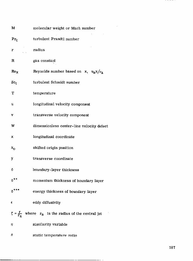
M molecular weight or Mach number
Prt
r
R
Re x
Sc t
T
U
W
X
X o
Y
77
turbulent Prandtl number
radius
gas constant
Reynolds number based on x, UaX/v a
turbulent Schmidt number
temperature
longitudinal velocity component
transverse velocity component
dimensionless center-line velocity defect
longitudinal coordinate
shifted origin position
transverse coordinate
boundary-layer thickness
momentum thickness of boundary layer
energy thickness of boundary layer
eddy diffusivity
where r a is the radius of the central jet
similarity variable
static temperature ratio
187
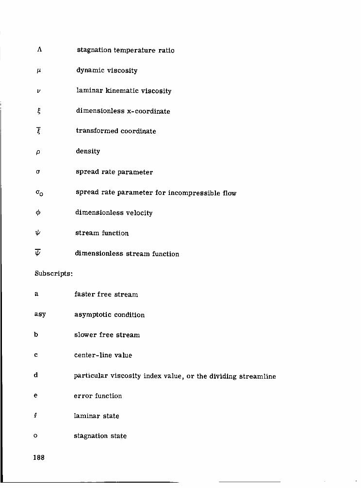
A stagnation temperature ratio
dynamic viscosity
laminar kinematic viscosity
dimensionless x- coordinate
transformed coordinate
P density
spread rate parameter
spread rate parameter for incompressible flow
dimensionless velocity
stream function
dimensionless stream function
Subscripts:
a faster free stream
asy asymptotic condition
b slower free stream
center-line value
d particular viscosity index value, or the dividing streamline
error function
laminar state
stagnation state
188
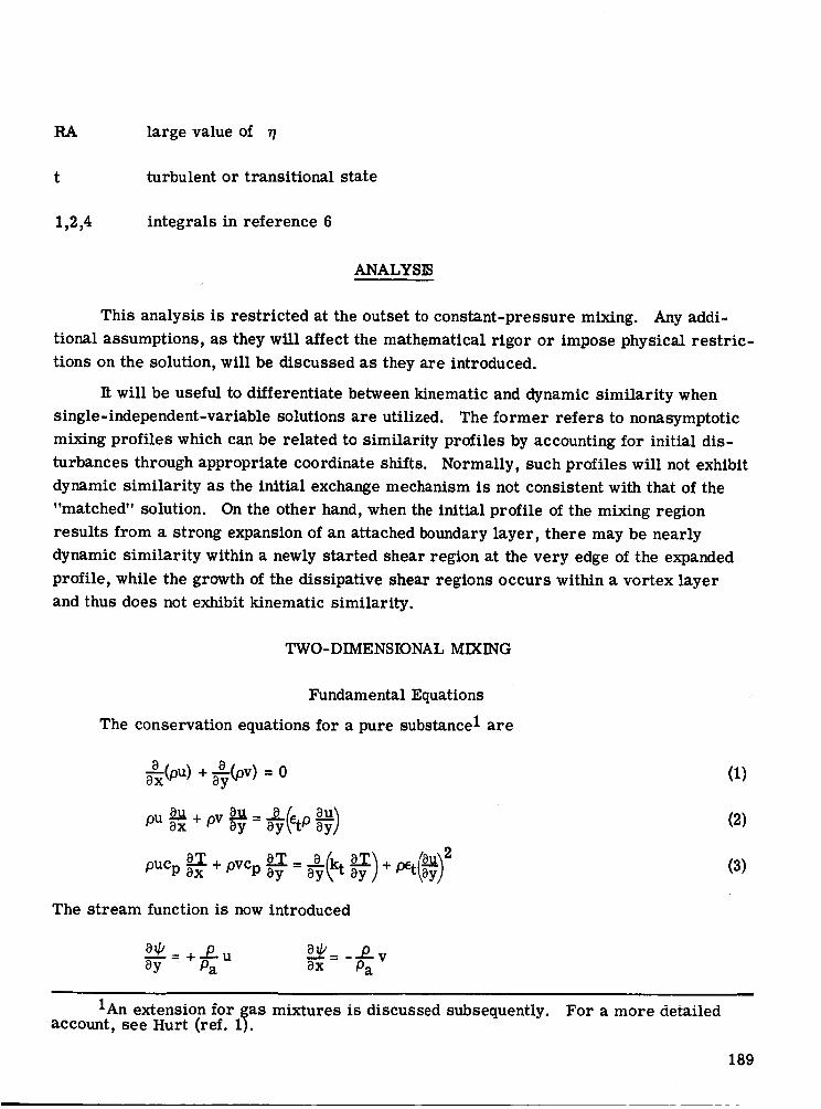
RA large value of
turbulent or transitional state
1,2,4 integrals in reference 6
ANALYSIS
This analysis is restricted at the outset to constant-pressure mixing. Any addi-
tional assumptions, as they will affect the mathematical rigor or impose physical restric-
tions on the solution, will be discussed as they are introduced.
It will be useful to differentiate between kinematic and dynamic similarity when
single-independent-variable solutions are utilized. The former refers to nonasymptotic
mixing profiles which can be related to similarity profiles by accounting for initial dis-
turbances through appropriate coordinate shifts. Normally, such profiles will not exhibit
dynamic similarity as the initial exchange mechanism is not consistent with that of the
"matched" solution. On the other hand, when the initial profile of the mixing region
results from a strong expansion of an attached boundary layer, there may be nearly
dynamic similarity within a newly started shear region at the very edge of the expanded
profile, while the growth of the dissipative shear regions occurs within a vortex layer
and thus does not exhibit kinematic similarity.
TWO-DIMENSIONAL MIXING
Fundamental Equations
The conservation equations for a pure substance 1 are
8 (_V _
tp
pUcpST 8T 8_ 8a_yy) _2_- + pVCp ay = _'_ t + _t
The stream function is now introduced
og, a-k =--P-v0"7 = + _a u 0x Pa
(1)
(2)
(3)
1An extension for gas mixturesaccount, see Hurt (ref. 1).
is discussed subsequently. For a more detailed
189

and new dimensionless variables defined
gb= u x _=_ 8- T _Pa (4)_aa _ = E uaL T a P
where _, related to the stream function @, is to be used as an independent variable in
the Von Mises plane. Accordingly, after introducing the free-stream Crocco number,
Ca 2 - Ua 22CpTo a
and accounting for the transport mechanisms by the kinematic viscosity
effective Prandtl number Prt, the following equations are obtained:
(5)
et = _t and theP
(6)
A far
7 2c 2_'_ _ _ rtLua _ + L"_al-Cq20-_-_/
reaching simplification of the analysis can be achieved by setting (ref. 2)
(v)
gt p(1-d) = f(_) (8)
where d = 1 - w (w being the exponent of the Sutherland equation for the dynamic vis-
cosity of a gas) corresponds to the laminar mixing problem.
The transformation
d_= 1 et d} (9)
ReL u _o2-d
then produces a pair of parabolic simultaneous partial differential equations which can be
solved without reference to any specific assumption concerning exchange mechanisms
(except d and Pr O. These equations are
1 8 (_._ ___) 2Ca 2 ___/_8_._2_= P-rt _ +1-Ca 2 0--_8-_)(11)
190

For given initial conditions, step-by-step integrations using implicit iterative pro-ceduresfor better convergence(see ref. 3) canbe carried out with the help of high-speeddigital computers.
in the form of _(_,_) and 0(_,_) and the coordinate y/L isResults appear
found from
(12)
Similarity Solutions
"Exact solutions".- By starting with equation (10) and following the development for
nonisoenergetic mixing of two uniform streams having identical compositions (ref. 4), an
effective Prandtl number of unity, and satisfying the boundary conditions
leads to
y -*-_, u - Ub, TO - Tob
y -* +_, u --Ua, T O --Ton
f'" IA- Ca2f'2_d ff"- d(A'- 2Ca2f'f '') f" -0 (13)+L1- J A-ca2,'2
-_,where f(7/) - g-_ f'0/) = _,
77 is the independent similarity variable defined by
_] -- -_g' (14)_1 rg
and primes
From the assumption of similarity, it follows that one may set
so that
_ = _ (15)
indicate differentiation with respect to the respective independent variable.
gg' = 1 _,
g(_')= _2"_ (16)
191

and the transformation to physical coordinates canbe accomplishedwith
1
By adoptingC_ertler's formulation (ref. 5) of
(17)
et _ 1 Re L _ (18)v_ 2"d 4ad 2
one obtains
2a d Y =,_" _ d_ (19)
where the origin of y is placed at the zero streamline where f(l)rT}" = 0. aThe notationad has been introduced to stress the fact that the similarity paramet= depends not
only on the procedure of matching between an experimental and an analytical profile but
also on the choice (if one is needed or indicated) of the analytical formulation (ref. 4).
An extension to analyze the mixing of two streams having different gas constants
R a and Rb is easily accomplished for Prandtl and Lewis numbers of unity by the
expression
Pa=p 1-1Ca2 _ Tv/2 _2C a (20)
(See discussion of test case 3, also.)
Error function solution.- Proposed as a first-order approximation for solving equa-
tion (10) under the conditions of incompressible flow with d = 0 by GSertler (ref. 5), the
error function distribution for the velocity profile is
1 - q_b err 7? (21)_b = 1(1+ _bb)+ m
where _ = ae(Y ). The error function solution has been widely used for momentum inte-
gral methods devised to deal with compressible, diabatic (ref. 6), and even reactive
(ref. 7) free shear layers. Auxiliary integrals for determining mass, momentum, and
energy transfer, as well as shear stress, dissipation rates, and property distributions,
have been tabulated (ref. 6) or made subroutines of more comprehensive programs deal-
ing with propulsion problems (ref. 8). A discussion of differences between spread rate
parameters (_e, ad, etc.) has been included in reference 4.
192

Initially Disturbed Mixing Region
Similarity solutions are reachedasymptotically as the influence of initial distur-bances (in velocity andproperty profiles andin the exchangemechanism)decreases.The gradual approachto similarity profiles canbe represented in its latest stagesby alateral shift of mixing profiles, that is, by satisfying the momentumintegrals. This stillleaves openthe questionof how to interpret properly similarity parameters suchas awhenthe exchangemechanism is to be evaluatedat other than far-downstream locations.Attention will be givento the latter problem in the section on "Eddy Viscosity Concepts."
Origin-shift methods.- Utilization of similarity solutions for initially disturbed
profiles by origin-shift methods has been suggested in different forms by various authors,
and the work of Hill and Page (ref. 9) and Kessler (ref. 10) may be consulted for further
details. Use of the momentum integral for determining lateral and longitudinal coordi-
nate shifts will, however, become unfeasible when wakes or mixing between streams of
nearly equal velocity in the presence of relatively large initial disturbances have to be
considered. It should be noted that virtual origins for exchange coefficient growth have
been found useful in connection with eddy viscosity models employed in finite-difference
integrations of the fundamental equations (see the section "Eddy Viscosity Concepts").
Local similarity.- The restriction on the type of viscosity models consistent with
the longitudinal coordinate transformation expressed by equation (9) will be found most
unrealistic for cases where a relatively thick boundary layer undergoes a rapid expan-
sion (such as in base flows) before the onset of constant-pressure mixing. This can lead
to effective quenching of the turbulence level in the expanded profile (which is then rota-
tional but not strongly dissipative) while the dissipative exchange mechanism remains
confined to a much narrower shear region (refs. 11 and 12). This shear region exhibits
features of local similarity and is initially laminar before undergoing transition. Growth
of such transitional shear regions, for single-stream mixing, has been analyzed in some
detail by Gerhart (ref. 13), and there seems to be confirmation that the similarity param-
eter _ retains its qualitative relevance and quantitative value. Since turbulent mixing
now appears to originate well downstream of the "expansion corner," agreement with
origin-shift methods concerning the energy levels of the dividing streamline is surprising
but can be supported by detailed calculations.
Numerical integrations.- Computer programs have been developed to perform the
step-by-step numerical integration of the system of equations (refs. 1 and 2), and an
implicit iterative method of integration is utilized which improves the economy of the
calculations while retaining accuracy and assuring numerical stability.
The integration uses initial and boundary conditions given in physical coordinates
x and y b,,t proceeds with calculations in the transformed _h-plane. Dimensionless
velocity (_P = _a), temperature (O = _-a), or density (p//Pa) distributions are then found as
193

functions of _ (or y/L) for parametric values of the variable 7. Location of the
value with the x-scale depends upon the viscosity law as contained in the transforming
equation (eq. (9)) which can be written
- 1 f e d x= Re---_ v_82-d L
Attempts have been made to gain information on the integrand by matching of calculated
and experimentally determined profiles, for example, by the dissipation integral (ref. 2)
or other unique features (such as minimum velocity in wakes). (See section concerned
with determination of the eddy viscosity.)
_o_- t.ke problems at hand, however, one needs this information as input, and cer-
tain speculative assumptions on the behavior of the turbulent eddy viscosity still are to
be specified in the section "Eddy Viscosity Concepts" in order to explain their use for
obtaining solutions to the test cases.
AXIALLY SYMMETRIC MIXING REGIONS
An extension of the theoretical analysis and the resulting computer program for jet
mixing dealing with axisymmetric geometries and nonhomogeneous gases has been made
by Hurt (ref. 1). Like many others (e.g., refs. 14 and 15), he utilizes the system of global
conservation equations as well as conservation of species without chemical reactions.
The simplifying assumptions are consistent with boundary-layer approximations but, in
addition, he assumes a turbulent Lewis number of unity which implies that the turbulent
Schmidt and Prandtl numbers are equal to each other yet not necessarily equal to unity
individually. Also, specific heats at constant pressures are assumed to be functions of
concentrations but not of temperature, which limits his analysis to moderate temperature
variations even though it attempts to cope with compressibility. In this sense, and with
regard to improved numerical integration procedures, Hurt's work is an extension of that
by Donovan and Todd (ref. 15). The resulting set of equations is in analogy with those of
the preceding sections except for the accounting for species and the use of a dimensionless
enthalpy rather than temperature in the energy equations:
0 _ 8c.i_l= _"_.F_';:'_.L'''t _2_:2_
a4 _-Ji=l (22)
ah = _2_a.._..._L_ a_
a_ a5 rt+
,N
1 - Ca 2
194

Here,m n
_u 1 _ v__= la_P Waa= _ _ _ Ua - _"o"_"
C a is the Crocco number of the internal stream, and _ = _ were r a is a reference.Uara
radius of the coaxial stream, _ = p_ and h = h, ha"
In addition, the perfect gas law for isobaric mixing of a multispecies mixture
= ! _ (23)yT
was utilized, where
N
N
i_l ca_i•= Mi
T = m.T The static temperatureTa
m
M i is the molecular weight of the ith species, and
ratio T was evaluated from the energy equation and then the stagnation temperature
ratio was found by using the following formulation developed from the relationship
between stagnation and static enthalpy:
(24)
(25)
where
N
_ CiCpi
_= i=l (26)N
CaiCpa ii=l
and A is the local stagnation temperature ratio. In contrast to the two-dimensional
case, the transformation of the streamwise coordinate _ (to eliminate the eddy viscosity
from the equation) was not included in Hurt's analysis. This was due to evidence that the
effective turbulent exchange coefficient could not be considered, with sufficient accuracy,
to be a L,.,ct .... of the streamw_,_ rnordinate only. His n_'n_rrnrn, thu_, can n.e.enmmodate
as input suitable eddy viscosity models. At this stage, however, there do not appear to be
195

sufficient experimental data and insight into controlling mechanisms to expect a simple
yet universal formulation for a phenomenological eddy viscosity model.
It is of interest to note the efforts of Spalding and his coworkers at Imperial College
(e.g., ref. 16) and others to gain a better insight into turbulent exchange mechanisms by
use of multiparameter models involving the kinetic energy of turbulent motion.
EDDY VISCOSITY CONCE PTS
Within the restrictions imposed by the coordinate transformation (eq. (9)) and the
resulting coupling of the viscosity to the density for two-dimensional mixing problems,
there is still the possibility of coping with fully laminar, fully turbulent, and transitional
cases. The initial conditions have first to be examined.
INITIAL CONDITIONS RELATED TO APPROACHING BOUNDARY LAYER
A mixing region can be the result of flow separation associated with
(i) Constant pressure (wake behind a flat plate)
(ii) An acceleration (as in the supersonic base pressure problem)
(iii) A pressure rise (due to an adverse pressure gradient)
In any one of these cases, the attached boundary layer will cause an initial disturbance
for the mixing region. Each case, however, will be different in its kinematic and dynamic
effects.
The constant-pressure case appears to be the simplest. One would expect that both
the flow profile and the viscous structure remain virtually unchanged. The acceleration
causes a change in the velocity profile (which could possibly be accounted for by a stream-
line expansion method), but it also tends to quench the turbulent mechanism (refs. 11
and 12). This can lead to the situation discussed in the section "Local Similarity" which
produces a transitional problem in a "mixing sublayer" imbedded in a vortex layer.
Separation associated with a pressure rise presents the most complicated problem
and points to the need for a momentum integral approach (ref. 17) and origin-shift treat-
ment of the mixing zone (e.g., ref. 10).
INITIAL EXCHANGE MECHANISMS
It is evident that a mere description of velocity, temperature, and concentration pro-
files will, in the turbulent case, generally not be sufficient to solve the problem of comput-
ing the development of the mixing region. What is missing could be most important - at
196
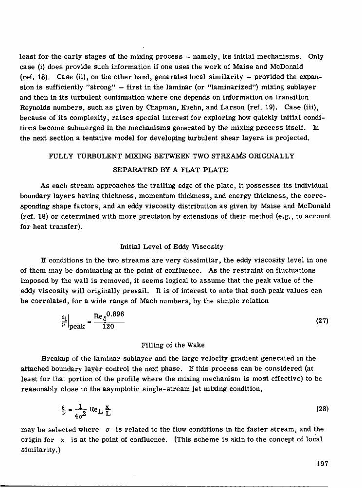
least for the early stagesof the mixing process - namely, its initial mechanisms. Onlycase (i) does provide such information if one usesthe work of Maise and McDonald(ref. 18). Case (ii), on the other hand, generates local similarity - provided the expan-
sion is sufficiently "strong" - first in the laminar (or "laminarized") mixing sublayer
and then in its turbulent continuation where one depends on information on transition
Reynolds numbers, such as given by Chapman, Kuehn, and Larson (ref. 19). Case (iii),
because of its complexity, raises special interest for exploring how quickly initial condi-
tions become submerged in the mechanisms generated by the mixing process itself. In
the next section a tentative model for developing turbulent shear layers is projected.
FULLY TURBULENT MIXING BETWEEN TWO STREAMS ORIGINALLY
SEPARATED BY A FLAT PLATE
As each stream approaches the trailing edge of the plate, it possesses its individual
boundary layers having thickness, momentum thickness, and energy thickness, the corre-
sponding shape factors, and an eddy viscosity distribution as given by Maise and McDonald
(ref. 18) or determined with more precision by extensions of their method (e.g., to account
for heat transfer).
Initial Level of Eddy Viscosity
If conditions in the two streams are very dissimilar, the eddy viscosity level in one
of them may be dominating at the point of confluence. As the restraint on fluctuations
imposed by the wall is removed, it seems logical to assume that the peak value of the
eddy viscosity will originally prevail. It is of interest to note that such peak values can
be correlated, for a wide range of Mach numbers, by the simple relation
et I Re50"896 (27)F peak = 120
Filling of the Wake
Breakup of the laminar sublayer and the large velocity gradient generated in the
attached boundary layer control the next phase. If this process can be considered Cat
least for that portion of the profile where the mixing mechanism is most effective) to be
reasonably close to the asymptotic single-stream jet mixing condition,
f-=4-_ReL_v (28)
may be selected where a is related to the flow conditions in the faster stream, and the
origin for x is at the point of confluence. (This scheme is akin to the concept of local
similarity.)
197

Approachingthe Asymptotic Solution
With the jet mixing mechanismthus building up, it will eventually approach theasymptotic case for both the kinematic and dynamic aspects.
At thematching conditions, after selecting anappropriate similarity profile, onehas to accountfor both the momentumand energy defects at x = 0.
This can be achieved by applying an origin shift x o and by utilizing the concept
of equivalent bleed (ref. 6). By using the integrals defined and tabulated in reference 6
for the error function profile, one relates the mechanical energy defect in the approach-
6a*** + _bb35b***ing streams at x = 0, D = 2 through
(-Xo)Ua3pa2_D= _I(_/RA)- ii@d_(1 - _b2) - I4(_RA )(29)
while the momentum defect is accommodated through the concept of equivalent bleed
which determines
where
I1( d)1 (30)
5b**Ab = p_ _b 2 (-Xo)
and
Combining equations (29) and (30) yields, for the origin shift,
The similarity parameter _ refers here to the two-stream case (ref. 6).
It is necessary to comment on the manner in which the asymptotic case is
"approached." If the "filling of the wake" (in the sense of the preceding section) becomes
pronounced due to _b > 0, the increase in eddy viscosity described by equation (28) will
initially prevail over that related to the asymptotic solution. Hence, an overshoot will be
198

experienced so that the approach to the asymptotic profile occurs in the sense of relaxa-
tion rather than amplification of the mixing mechanism.
For the case where _b = 0, such an overshoot should be less pronounced. The
energy defect integral, as utilized for determining the origin shift Xo, differs from the
dissipation integrals defined in reference 2)
or
j.+o DI = (1- ¢)C_b- _bb)d_ (33)
only by a constant value (due to the fact that the momentum of the mixing streams is pre-
served once external forces such as wall shear friction are not present). The dissipation
integral has been evaluated and presented in graphical form as shown in figure 1 for a
variety of flow conditions.
Use of both forms (eq. (32) for the experimental profile and eq. (33) for the analyti-
cal solution) is then convenient for establishing the relation between x/L and [ and
E/v(x/L).
Wake Problem - Both Streams Having Identical Velocities
and Initial Boundary Layers
For wake flows, the asymptotic solution shall be represented by a constant level of
the eddy viscosity (Schlichting (ref. 5)) so that, with reference to the momentum thickness
of one approaching boundary layer,
6a**_-v= 0"0888ReL L (34)
Proposed Models for Turbulent Eddy Diffusivity
A schematic presentation of eddy viscosity models as used in the present study is
shown in figure 2.
RELATION BETWEEN THE STREAMWISE COORDINATES x AND
The proposed eddy viscosity model establishes a relation between the transformed
coordinate _ and the physical coordinate x, and thus allows identification and location
of the calculated mixing profiles
199

_=_ e 1 d(__)+Constant (35)v82-d Re L
DETERMINATION OF THE EDDY VISCOSITY FROM MATCHING OF
EXPERIMENTAL AND ANALYTICAL PROFILES
The concepts developed for e/v in the preceding sections are essentially conjec-
tures. Indeed, the analytical model and the calculation procedures have been worked out
in such a way as to remove the need for depending on a specific viscosity law. Actually,
one can utilize equation (9) for determining the viscosity law.
To accomplish this, it is necessary to define the matching of profiles for value
pairs of x and _, which leads to a unique "_ = :_(x) relationship which then can yield,
for d = 2
_'=-_]vd( x ReL (36)Ex
Obviously, only single parameters can be matched for both the calculated and the experi-
mental profiles.
Two possible choices are
(i) The minimum velocity, as it is well defined in wake problems
(ii) The dissipation integral given by equations (29), (32), and (33)
An illustration of this procedure is given in the section "Test Case - Solutions."
EDDY VISCOSITY IN AXIALLY SYMMETRIC MIXING REGIONS
Much uncertainty exists concerning suitable turbulent exchange coefficient formula-
tions for axially symmetric flow. The appearance of the transverse coordinate r in the
conservation equations also complicates the situation since it would restrict the possibili-
ties of a transformation (e.g., eq. (9) for the two-dimensional case) to the unattractive
form where a singularity in the exchange coefficient could occur as r -- 0. Empirical
relations, therefore, still are favored in dealing with individual cases (ref. 1) but appar-
ently cannot be expected to give satisfactory results when applied to widely different flow
conditions. (See discussion of test case 11.)
200

TEST CASE - SOLUTIONS 2
TEST CASE 1: TWO-DIMENSIONAL SHEAR LAYER
Spreading Parameter for a Fully Developed Incompressible Free Shear
Layer (Influence of _b)
The effect of the free-stream velocity ratio ub = the spreading parameterUa 4_o on
for similarity mixing profiles has recently been reviewed by Yule (ref. 20). Shown in
figure 3 is the relation
as presently used in computer programs at the University of Illinois and which also has
been utilized for calculations of asymptotic mixing regions in the discussion of test
case 4.
TEST CASE 2: TWO-DIMENSIONAL SHEAR LAYER
Spreading Parameters for a Fully Developed Turbulent Free Shear Layer With
Zero Velocity Ratio (Influence of Mach Number)
Much uncertainty exists as to the effects of Mach number on the mixing mechanism,
as can be illustrated by the large discrepancies for observed or predicted values for a
(ref. 9). Shown in figure 4 is the simple linear relationship
a=12 +2.76M a
as proposed for use in the lower Mach number range Ma < 3 (ref. 6).
TEST CASE 3: TWO-DIMENSIONAL SHEAR LAYER
Spreading Parameter for a Fully Developed Low-Speed Free Shear Layer With
a Velocity Ratio of 0.2 and Density ratios pb/p a o£ 14, 1/2, 1/7, and 1/14
It is the judgment of the authors that conclusions concerning spread parameters
must be based on more extensive and reliable experimental data than appears to be pres-
ently available. Evaluation of earlier experiments by Pabst (ref. 21) conducted for a sin-
gle temperature ratio of 2.3 did not show an appreciable effect on a. To facilitate future
correlations, theoretical calculations for ad(AY/X) based on the procedure outlined in
the section "Similarity Solutions" with a selected value for d = 2 are presented in fig-
ure 5. The abscissa in figure 5 represents either the ratio of Tb/T a or pa/p b since
2 d = 2 for all calculations presented.
201
low-speed flows are being considered. According to equation (20), the effects of the
stagnation temperature ratio and gas constant ratio should be equivalent.
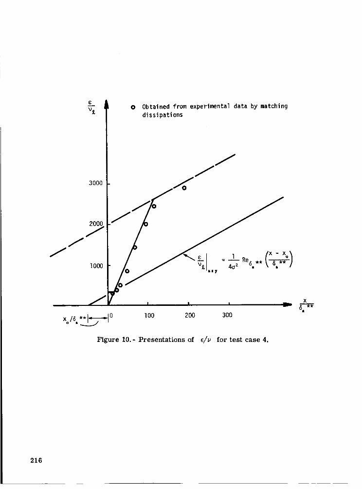
TEST CASE 4: TWO-DIMENSIONAL SHEAR LAYER
Influence of Initial Boundary Layers, Incompressible Flow, (bb = 0.35
As requested, results of theoretical calculations for the velocity profiles are shown
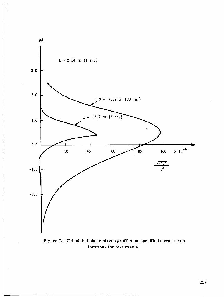
in figure 6. The corresponding shear stress distributions are given in figure 7. The
correlation procedure between the physical and transformed dimensionless streamwise
coordinates x/L and _ is illustrated by the use of the dissipation integrals according
to equations (32) and (33) in figures 8 and 9. The extracted information on the effective
turbulent eddy viscosity e/v is shown in figure 10.
This figure also compares these viscosity coefficients with those resulting from
the concepts developed in the section "Eddy Viscosity Concepts." A strong overshoot as
a continuation of the wake-filling mechanism over the asymptotic solution is clearlyevidenced.
TEST CASE 5: TWO-DIMENSIONAL SHEAR LAYER
Initial Development of a Turbulent Compressible Free Shear Layer
The requested theoretically calculated velocity profiles are shown in figure 11.
One must note that the y-scale in figure 11 reflects conservation of momentum, while
the experimental data require a translation to satisfy this physical constraint. Fig-
ures 12 and 13 have been added to show the degree of agreement between the eddy vis-
cosity distributions based on the dissipation integral correlation and the concepts pro-
posed in the section "Eddy Viscosity Concepts." Again, an overshoot is noted, but it is
rather moderate since no wakelike contribution exists for _bb = 0.
TEST CASES 6 TO 13, 15, AND 17 TO 23: AXIALLY
SYMMETRIC FLOW CASES
Considerable difficulty has been encountered in attempts to obtain numerical com-
puter solutions by using the approach and programs of reference 1. This situation has
been caused primarily by communication problems (Dr. Hurt had left the University of
Illinois) and by difficulties encountered in switching to a different computer system with
limited storage capacity. Consequently, attention is directed to reference 1 as containing
specific examples for program capabilities. In addition, calculated center-line velocity
distributions as they apply to test case 11 are shown in figure 14.
202

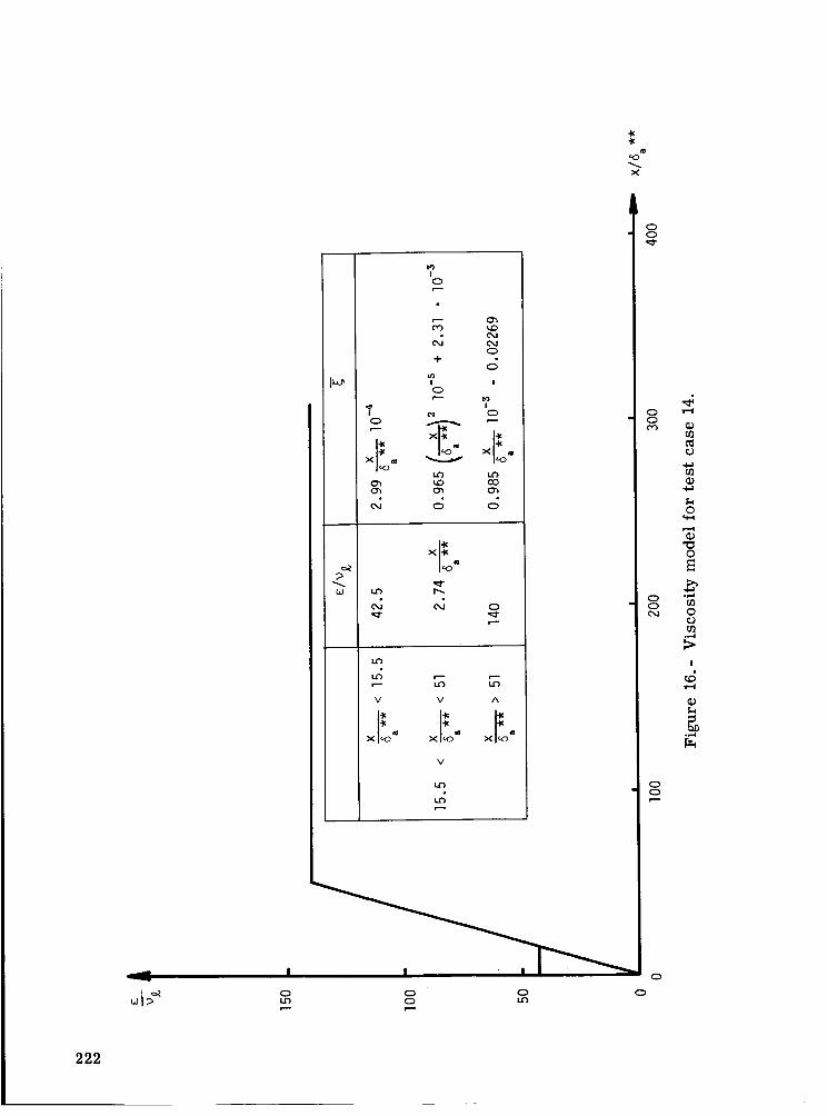
TEST CASE14: TWO-DIMENSIONALWAKE - LOWSPEED
Shownin figure 15 is the center-line velocity developmentas a function of thetransformed coordinate _. Figure 16 illustrates the use of the presently proposedviscosity model for the three regimes described previously. This produces the plotof 1/W2 as a function of X/Sa** (fig. 17),which is the required answer to this testcase. Agreement with experimental datawas foundto be reasonably good.
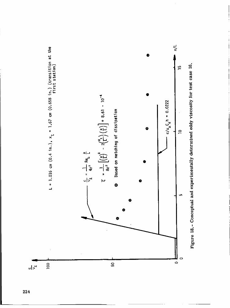
TEST CASE 16: TWO-DIMENSIONAL WAKE - SUPERSONIC
ADIABATIC FLOW
With transition at station 1, the present viscosity model assumes the form shown
in figure 18 with experimental e/v values (obtained with the help of dissipation function
correlation) also presented. A strong overshoot along the trough-concept-rise is noticed
with subsequent relaxation towards the asymptotic (constant e) solution. It must be noted
that the theoretical calculations for 1/W 2 as a function of x/D (fig. 19 (required))
and Tc/T a as a function of x (fig. 20) have been obtained by following the trough-rise
portion. The difference between the "relaxing" and the "rising" e/v branch should, how-
ever, not produce significant differences, especially in view of the rather large scatter of
experimental data. Overshoot and subsequent relaxation of e/v is experimentally -
albeit indirectly - evidenced by figure 1 of reference 22. Computer results (_bc and
Tc/T a as a function of _) are presented in figure 21.
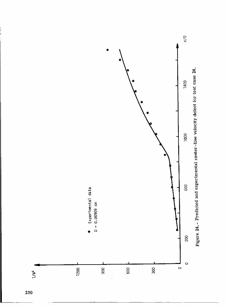
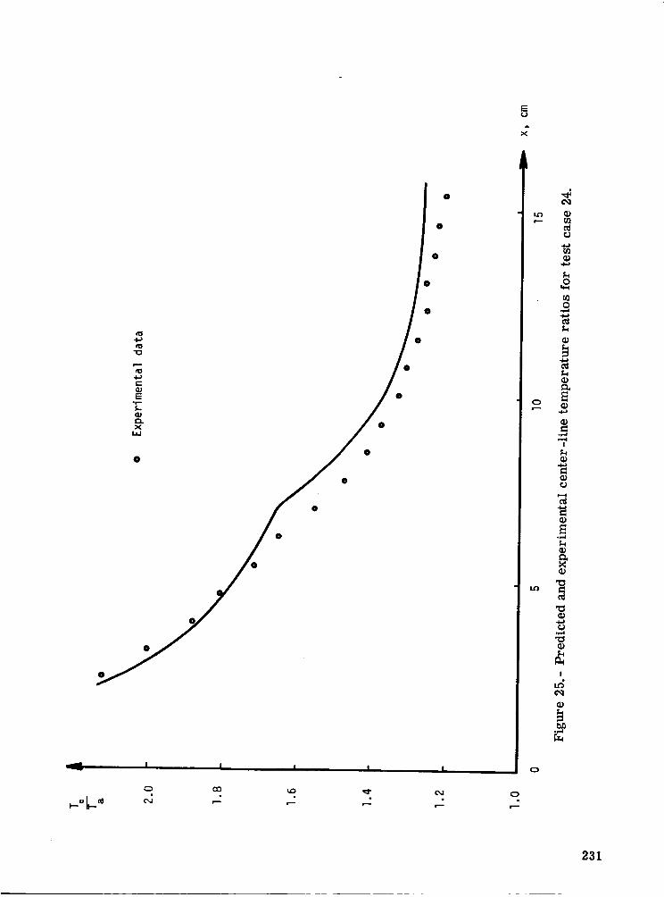
TEST CASE 24: TWO-DIMENSIONAL WAKE - COMPRESSIBLE
DIABATIC FLOW (TRANSITIONAL)
Prandtl number for this case has been selected as 0.72 throughout. This is con-
sistent with the expectation of a significantly long laminar mixing region followed by
transition and turbulent mixing for which Pr t = 0.72 is incidentally a reasonable
approximation. Based on theoretical calculations, and with the use of information on
transition in free shear layers (ref. 19), one arrives at a transition location of 7.01 cm
(2.76 in.) corresponding to Re x = 180000 where
Re x = ReL(Xt/L)t
The resulting relation between e/v and
between
lations (_c,
x/L is shown in figure 22. Correlation
and x/L by the integration of equation (9) and the finite-difference calcu-
function of _ in fig. 23') then produce figure 24 which showsTc/Ta as a/
203
1/W2 as a function of x/D and figure 25which is a comparison of calculated and mea-sured center-line temperature ratios. It is of interest to note the effects of transitionas they appear in both the calculated and experimentally determined data.
204

REFERENCES
1. Hurt, Robert Frank: A Theoretical and Experimental Investigation of Axisymmetric,
Non-Homogeneous, Compressible Turbulent Mixing. Ph.D. Thesis, Univ. of
Illinois at Urbana-Champalgn, 1970.
2. Lilienthal, Peter Frederick, H: Development of Viscous Free Shear Layers Between
Two Compressible Constant Pressure Isoenergetic Streams With Special Consid-
erations of Its Dissipative Mechanisms. Ph.D. Thesis, Univ. of Illinois, 1970.
3. Grabow, Richard M.: Finite Difference Methods. Laminar Separated Flows, VKI
CN 66a, Yon Karman Inst. Fluid Dyn., Apr. 1967.
4. Korst, H. H.; and Chow, W.L.: On the Correlation of Analytical and Experimental
Free Shear Layer Similarity Profiles by Spread Rate Parameters. Trans. ASME,
Ser. D: J. Basic Eng., vol. 93, no. 3, Sept. 1971, pp. 377-382.
5. Schlichting, Hermann (J. Kestin, transl.): Boundary Layer Theory. Fourth ed.,
McGraw-Hill Book Co., Inc., c. 1960.
6. Korst, H. H.; and Chow, W.L.: Non-Isoenergetic Turbulent (Pr t = 1) Jet Mixing
Between Two Compressible Streams at Constant Pressure. NACA CR-419, 1966.
7. Davis, Lorin R.: Experimental and Theoretical Determination of Flow Properties in
a Reacting Near Wake. AIAA J., vol. 6, no. 5, May 1968, pp. 843-847.
8. Addy, A. L.: Thrust-Minus-Drag Optimization by Base Bleed and/or Boattailing.
J. Spacecraft & Rockets, vol. 7, no. 11, Nov. 1970, pp. 1360-1362.
9. Hill W. G., Jr.; and Page, R.H.: Initial Development of Turbulent, Compressible,
Free Shear Layers. Trans. ASME, Ser. D: J. Basic Eng., vol. 91, no. 1, Mar.
1969, pp. 67-73.
10. Kessler, Thomas J.: Two-Stream Mixing With Finite Initial Boundary Layers.
AIAA J., vol. 5, no. 2, Feb. 1967, pp. 363-364.
11. Page, R. H.; and Sernas, V.: Apparent Reverse Transition in an Expansion Fan.
AIAA J., vol. 8, no. 1, Jan. 1970, pp. 189-190.
12. Korst, H. H.: Dynamics and Thermodynamics of Separated Flows. Review Lecture
presented at 1969 International Seminar on Heat and Mass Transfer in Flows
With Separated Regions and Measurement Techniques (Herceg-Novi, Yugoslavia),
Sept. 1969.
13. Gerhart, P. M.: A Study of the Reattachment of a Turbulent Supersonic Shear Layer
With the Closure Condition Provided by a Control Volume Analysis. Ph.D.
Thesis, Univ. of Illinois,1971.
205

14. Libby, Paul A.: Theoretical Analysis of Turbulent Mixing of Reactive GasesWithApplication to SupersonicCombustionof Hydrogen. ARSJ., vol. 32, no. 3, Mar.1962,pp. 388-396.
15.Donovan,Leo F.; and Todd, Carroll A.: Computer Program for Calculating Isother-mal, Turbulent Jet Mixing of Two Gases. NASATN D-4378, 1968.
16. Rodi, W.; and Spalding,D. B.: A Two-Parameter Model Turbulence, and Its Applica-tion to Free Jets. W_irme-undStoffiiberstragung, vol. 3, no. 2, 1970,pp. 85-95.
17.White, Robert A.: Effect of SuddenExpansionsor Compressions on the TurbulentBoundaryLayer. AIAA J., vol. 4, no. 12,Dec. 1966,pp. 2232-2234.
18. Maise, George;and McDonald,Henry: Mixing Length and Kinematic EddyViscosityin a Compressible BoundaryLayer. AIAA J., vol. 6, no. 1, Jan. 1968,pp. 73-80.
19. Chapman,Dean R.; Kuehn,Donald M.; and Larson, HowardK.: Investigation of Sep-arated Flows in Supersonicand SubsonicStreams With Emphasis on the Effect ofTransition. NACARep. 1356, 1958.
20. Yule, Andrew J.: Spreadingof Turbulent Mixing Layers. AIAA J., vol. 10, no. 5,May 1972,pp. 686-687.
21. Szablewski,W.: Turbulente Vermischung ebener Heissluftstrahlen. Ing.-Arch.,Bd. XXV, Heft 1, Jan. 1957,pp. 10-25.
22. Demetriades, Anthony: Observationson the Transition Process of Two-DimensionalSupersonicWakes. AIAA Paper No. 70-793, June-July 1970.
206

7,
Id,°l, I
oo
o°,,-i4_1
o
o ,._
0
.
o 0
sen(el<i>)(q<i>-<i>)(<i>-L)S (_/o) = [_
J/l/1 "'<_ ._ <_
o ._
(_/_),J. (<'>.j.-,j.)(,:l.-L) S : Ia
<_ <3 <d>
,:,! I:1
"y lio
_ °,.-t
,-to
.,.'-I
_ ,.--i.,-t
U3
o
°_.,,I
0
m
!
(_iun),_ t ,_-,_)(,_-_),_ =_
207

lly developed "similar"
Shifted jet mixing
I I or,y ._/ I//f-T='_i-_°°c_°_:"_'_
I--Xo_J = x/,L
(a) Turbulent free jet mixing.
--Trough-Concept-Rise
f Fully developed wake
Wall boundary layer
(b) Turbulent wake flow.
Figure 2.- Viscosity model.
--- x/L
208

O
II
O
O
O
O
O
CM
O
O
O
E• F,,,I
Q
Oor.4
O
!
oF,,,I
209

2O
10
I //
o = 12 + 2.76Ma
I I I _ Ma0 2 4 6
Figure 4.- Influence of free-stream Mach number on
similarity parameter (T.
210

0
__ e--
I
0
I
i i I0
I I I I
0
I
I
io _
0
0
0
0
0
0
P4
II
0 _
!
_ 0
0
!
M
211

Y/L
3.0
2.0
l.O
0.0
-l.0
-2.0
I
0 0.2
L = 54 cm |2. (l in.)
Ix = 12.7 cm (5 in.) _-= 0.0186
x 76.2 cm (30 in.) T = 0.64 I
y 0 dividing streamline /III
xom\/j
I I
• ° .0
Figure 6.- Calculated velocity profiles at specified downstream
locations for test case 4.
212
yA-
3.0
2.0
L = 2.54 cm (l in.)
x = 76.2 cm (30 in.)
X _
l.O
0.0
f 20 40
12.7 cm (5 in.)
60 80 lO0 x lO"4
-l.0I
2
U!
v
-2.0
Figure 7.- Calculated shear stress profiles at specified downstream
locations for test case 4.
213

00
,-4
0
J i i I I0
I , I , I I I i I I I
0
0
0
m 0
i
0_,._
o
oow,-4
ow,-d
0
'_ 0
o
o
!
°_,,I
214

op-)
.0
oc_j
o
--I
><
_.. i l I I i ,I o
• • , •
0
t==-4
c0
.,=.4
.,-4
oCo
•:..=i
°_.=_,.='.4
• °f=4
o
Q_
0C.)
!
215
E0 Obtained from experimental data by matching
dissipations
3oooi
• , Y : _ Re(sa ** ('_]*)*-I
XoI_,'_l_1----I° IOO 200 300
Figure 10.- Presentations of e/u for test case 4.
216

Y/L
l.O
0.75
O.50
L = 2.54 cm (I in.)
x = 5.56 cm (2.19 in.)
x = 20.96 cm (8.25 in.)
= 0.005
--0.0505
0.25x = 5.56 cm
0.0 | I0 0.4 0.6 0.8 1.0
-0.25
X = 20,96 cm
-0.50
-1.00
Figure 11.- Calculated velocity profiles at specified downstream
locations for test case 5.
217

.._1
X
o o c; o o c;
co
0
r/l
0
[/l
b_
00_
0°p,d
L_0_
*'6
.o
t_
0o
i
e4
ID
218

,,_J
x
0
0
0
oO
\ II
×oi_
c: xl..J
°i---
•_ aJr,,e"0
•I,,) II_,.
\ _
\" \
°\\
Io
X
I I
0 cO
.,1.
l'l0_
V
EU
II
,.,=J
O_ _'--•r- II
"'-- 0
0
\ \\\
I I I
\\
U
0
0,p,,_
!
0p,d
0
o
219

X
ol.•'..l -.=l
I
0
rl=
l
iI
,IO
..a
..,1Q.
Q0
0
II
W
0 O
I I
II II
I I I I_
e- c-o o
•_ "o
I I I
@,4('_
C"J
CO
0
C_
O)C_
f_0
°_,-4
0p,-4
I
I
'r'-4
220

\\.
I I I I I i ,I I,Q br_
r=..,
i
r--,
Q
QI
m
m
w
u
m
p==o
_ o
- o
o
cQQ;
0
0,F-t
0
Q;p.
°F-I
!
Q;
Q;
Q;
I
Q_
221
r.O m
X
I0r--
O_O_
¢xJ
I0r--
,-- C_
¢xJ0
+
0
.- ?
Xc,o I
_.) cO
w L_ t_
cd 0
_4r-,
V V A
I luX X
v
_4
0 0 0 Q
00
r/l
0
o
c,J 0C;
!
00
0
222

-Ic4c
X
I.,') _1" (',') L'M P"
223
¢-.
0 ,_..-_
4J 0
•_, "_
0r-
5
+
II
X
e.-.p-
EU
0
..I
I00
e
+ _
xl._ ",- 0
UXl.--J e_ "_
1,_ I_ o
II n i_
,,,I_ _ •0
• •
I
O
-m
t_
!
+!8
I
Q
224

I/W 2
1500
1200
900
600
300
• Experimental Data
D = 0.00909 cm
@
01 I I I
200 400 600 800 1000
Figure 19.- Predicted and experimental center-line velocity
defect for test case 16.
1200 x/D
225

Tc
T-a
1.7
1.6
1.5
1.4
1.3
1.2
l.l
1.0
• Experimental data
I I ! I I
0 2 4 6 8 10
Figure 20.- Predicted and experimental center-line temperature
ratio for test case 16.
v
x, cm
226

I
///
\\
\
0
\\
I
CO
I I
227

=.I
X
0
W
!0
0
+
Xl_ X _
V I
×.-!
r.- X
e_
X *,j X *_
v A
X X
228

ii
i... Q
c_J
Oh
0
CO
rm
kO
rm
_q
co
r---
C_J
r--.
rm
o
c_
o
o
o
c)
c_
O
O
c_
O°p,,I
Q;
c_
OP-,I
'T
C.)!
c_
229
x
%
•r- O
X
It
• ""
0
I I I I
o
o
O O O OO O O O
O
CD
oCD
CD
O
O
g
o
OO
o
CJCD
"O
O
_D
CD
I
CD
CD
CD
(D
CD
°F-4"oCD
I
CD
bD
230
EU
I I I I
c)
r,-.
q_
0
r_0
q,)
q_
q_
°l,..d
_4
'el
"CS
°r.,4
"0
I
b_.i,-.f
231

DISCUSSION
Professor Goldschmidt: I am sorry, I must not have understood very well. How did you
define your shift in the origin - this x o - is it completely arbitrary or is it computed
somehow?
W. L. Chow: No, first I said it is a matching of energy defect of the mean flow of the
actual mixing profile to a fictitious one with a shifted origin, and meanwhile we have to
also apply an equivalent bleed concept. In other words, if we have an initial boundary-
layer flow, we always have a developing flow even far downstream. The flow looks sim-
ilar, still shifted somewhat, so we have to use the initial boundary-layer effect to corre-
late it and we call that an equivalent bleed concept. It is described in the paper and it is
long so I would rather not go into it at this time. If you would like to discuss anything
else I would be glad to answer your question in detail, in private.
232