ENVIRONMENTAL TRUST FUND

Nassir El‐Jabi and Gabriel GoguenUniversité de MonctonMoncton, NB

Daniel CaissieDepartment of Fisheries & OceansMoncton, NBMARCH 2019

ANALYSIS OF FLOOD TRENDS UNDER 

CHANGING CLIMATE INCLUDING FLOOD MAGNITUDE, 

VOLUME AND DURATION FOR NEW BRUNSWICK

PHASE I: The Miramichi Rivers System case study

  

 

 

 

Analysis of flood trends under changing climate including 

flood magnitude, volume and duration for New Brunswick  

PHASE I: The Miramichi Rivers System case study 

 

By 

 

Nassir El‐Jabi and Gabriel Goguen 

Université de Moncton, Moncton, NB 

 

 

and 

Daniel Caissie 

Department of Fisheries & Oceans, Moncton, NB 

 

March 2019

  

 

 

 

 

 

 

 

 

 

 

 

 

 

 

This page intentionally left blank. 

 

 

 

 

 

 

 

 

 

 

 

 

 

 

 

 

  

 

 

 

 

 

 

 

 

 

 

 

 

 

 

 

 

 

 

 

 

 

 

Warning: Neither  the  organizations  named  in  this 

Report, nor any person acting on behalf of 

any  of  them,  assume  any  liability  for  the 

misuse  or  misunderstanding  of  the 

information  presented  in  this  study.  The 

user is expected to make the final evaluation 

of the appropriateness of the technique and 

the accuracy of the data and calculations in 

his or her own set of circumstances. 

Avertissement: Les  organisations  énumérées  dans  ce 

rapport ou toute personne agissant en leurs 

noms déclinent toute responsabilité pour le 

mauvais  emploi  ou  la  mauvaise 

interprétation  des  renseignements 

contenus dans cette étude.  Il  incombe aux 

utilisateurs  d’évaluer  la  pertinence  des 

techniques  et  l’exactitude  des  données  et 

calculs  dans  les  circonstances  qui 

s’appliquent

 

  

TABLE OF CONTENTS 

LIST OF TABLES ........................................................................................................... 1 

LIST OF FIGURES .......................................................................................................... 2 

LIST OF ACRONYMS AND SYMBOLS ......................................................................... 3 

ABSTRACT ..................................................................................................................... 4 

RÉSUMÉ ......................................................................................................................... 5 

PREAMBLE .................................................................................................................... 6 

1.  INTRODUCTION ..................................................................................................... 7 

1.1  Phase I (2018‐2019): .............................................................................................. 7 

1.2  Phase II (2019‐2020): ............................................................................................. 8 

2.  BACKGROUND .................................................................................................... 10 

2.1  Deterministic methods of estimating flood flows.............................................. 10 

2.2  Stochastic methods of estimating flood flows ................................................... 10 

2.3  Annual maximum series approach ..................................................................... 10 

2.4  Annual maximum series distribution ................................................................. 11 

2.5  Peak over threshold ............................................................................................ 11 

2.6  Peak over threshold – Selection of threshold value .......................................... 11 

2.7  Peak over threshold – Occurrence distribution ................................................. 12 

2.7.1  Independence criteria ......................................................................................... 12 

2.8  Peak over threshold – Exceedance distribution ................................................. 12 

2.9  Flood volume and duration ................................................................................. 12 

3.  METHODOLOGY .................................................................................................. 13 

3.1  Flood frequency analysis ..................................................................................... 13 

3.2  The GEV distribution function used in the AMS approach ................................ 13 

3.3  Distribution of the occurrence of floods in the POT analysis ............................ 14 

3.4  Selection of threshold values .............................................................................. 15 

3.5  Independence criterion ....................................................................................... 15 

3.6  Distribution of the magnitude of flood exceedances ........................................ 16 

  

3.7  Distribution of flood volumes and durations ..................................................... 18 

4.  STUDY AREA AND DATA ................................................................................... 20 

4.1  Choice of hydrometric stations and detailed analysis of streamflow data ....... 20 

5.  RESULTS AND DISCUSSIONS ........................................................................... 25 

5.1  AMS Flood magnitude ......................................................................................... 25 

5.2  POT Flood magnitude .......................................................................................... 25 

5.3  Independence criterion ....................................................................................... 36 

5.4  Flood volume ....................................................................................................... 38 

5.5  Flood duration ..................................................................................................... 41 

6.  CONCLUSIONS .................................................................................................... 46 

AKNOWLEDGEMENTS ................................................................................................ 47 

REFERENCES .............................................................................................................. 48 

  1  

LIST OF TABLES Table 1 : Treshold values and true mean number of exceedance per year (MNEY) for the 

Miramichi River stations ............................................................................................................... 15 

Table 2: Miramichi River station names and characteristics ........................................................ 23 

Table 3: Calculated discharge (m3/s) for different return periods using the AMS‐GEV model .... 25 

Table 4: Calculated discharge (m3/s) for varying mean number of exceedances per year for 

different return periods using the POT‐GP model ........................................................................ 27 

Table 5: Calculated discharge in (m3/s) for varying mean number of exceedances per year for 

different return periods using the POT‐Exp model ....................................................................... 30 

Table 6: Average duration (days) per flood event for different MNEYs ....................................... 41 

 

 

 

 

 

 

 

 

 

 

 

 

 

 

 

 

 

 

 

 

 

 

 

 

  2  

LIST OF FIGURES Figure 1: Flow hydrograph with identification of flood characteristics……………………………………..14 

Figure 2: Hierarchical clustering of NB gauged hydrometric stations .......................................... 21 

Figure 3: Map of gauging stations, as well as their group and rank. Names of inactive stations 

are shown in gray. ......................................................................................................................... 21 

Figure 4: Miramichi watershed with location of hydrometric stations (black dot) and assigned 

catchment area (colored areas) .................................................................................................... 24 

Figure 5: Fitted distribution for the annual maximum series approach (AMS‐GEV) using the GEV 

model in relation to the observed annual maximum values ........................................................ 26 

Figure 6: Fitted high flows for different return periods using the POT‐GPD model for MNEY of 

1.0, 1.5, 2.0 and 3.0 and AMS‐GEV in relation to observed annual maximum values ................. 29 

Figure 7: Fitted high flows for different return period using the POT‐Exp model for MNEY of 1.0, 

1.5, 2.0 and 3.0 and AMS‐GEV in relation to observed annual maximum values ........................ 31 

Figure 8: Variation of QT for different MNEYs for different return periods at the Southwest 

Miramichi River station ................................................................................................................. 32 

Figure 9: Variation of QT for different MNEYs for different return periods at the Little Southwest 

Miramichi River station ................................................................................................................. 33 

Figure 10: Variation of QT for different MNEYs for different return periods at the Northwest 

Miramichi River station ................................................................................................................. 34 

Figure 11: Variation of QT for different MNEYs for different return periods at the Catamaran 

Brook station ................................................................................................................................. 35 

Figure 12: Difference in calculated QT when applying a 6‐day interarrival independence criterion 

(see text for details) ...................................................................................................................... 37 

Figure 13: Average specific flood volume per year for different MNEYs ...................................... 38 

Figure 14: Fit of calculated flood volume distribution to annual maximum volume observations 

for POT‐GP‐1 and POT‐Exp‐1 ........................................................................................................ 39 

Figure 15: Total flood volumes per decade for MNEYs of 1, 1.5, 2 and 3 ..................................... 40 

Figure 16: Total flood volumes per decade for MNEY of 1 ........................................................... 41 

Figure 17: Average yearly duration of floods for varying MNEY ................................................... 42 

Figure 18: Fit of calculated flood duration distribution to annual maximum duration 

observations for POT‐GP‐1 and POT‐Exp‐ ..................................................................................... 43 

Figure 19: Total flood durations per decade for MNEYs of 1, 1.5, 2 and 3 ................................... 44 

Figure 20: Total flood duration per decade for a MNEY of 1 ........................................................ 45 

 

 

 

 

 

 

 

 

  3  

 

LIST OF ACRONYMS AND SYMBOLS AMS    Annual maximum series 

BM    Block maxima 

Exp    Exponential distribution 

GEV    Generalized extreme value 

GP    Generalized Pareto distribution 

MNEY    Mean number of exceedances per year 

POT    Peak over threshold 

 

DT_Exp    Duration of flood calculated with the POT‐Exp model for return period T 

DT_GP    Duration of flood calculated with the POT‐GP model for return period T 

F(x)    Cumulative annual maximum probability function 

H(x)    Exceedance distribution function 

n    Number of events in a given year 

P(n)    Arrival rate probability function 

QR    Threshold discharge 

QT_Exp    Discharge value calculated with the POT‐Exp model for return period T 

QT_GP    Discharge value calculated with the POT‐GP model for return period T 

T    Return period 

VT_Exp    Volume of flood calculated with the POT‐Exp model for return period T 

VT_GP    Volume of flood calculated with the POT‐GP model for return period T 

x    Discharge above threshold for probability F(x) 

 

α    Generalized Pareto distribution scale parameter 

β    Exponential distribution parameter 

ε    Generalized extreme value distribution shape parameter 

κ    Generalized Pareto distribution shape parameter 

λ    Poisson distribution parameter 

η(t)    Distribution of the number of exceedances in (0,t] 

σ    Generalized extreme value distribution scale parameter 

τ(i)    Time of arrival of ξi 

μ    Generalized extreme value distribution location parameter 

ξ    Magnitude 

 

 

 

 

 

 

  4  

ABSTRACT  

  The planning and construction of hydraulic control structures,  the operation of reservoirs and the improvement of flood forecasting techniques all require an effective estimation of floods.  Notably,  the  quantification  of  floods  must  be  as  accurate  as  possible  to  avoid overdesign of hydraulic  structures or  to prevent under designs, which could  result  in  the failure  of  structures  with  the  potential  loss  of  human  lives.  To  achieve  this  objective,  a statistical  analysis  of  floods  is  the  preferred  approach  for  estimating  floods  of  various frequencies.  This analysis generally consists of fitting high flows to distribution functions and then  estimating  floods  for  different  recurrence  intervals.  The  classic  approach  to  flood frequency analysis is the Annual Maximum Series (AMS) analysis, which consists of fitting the maximum discharge of every year to a distribution function.   Numerous studies have already been carried out, to estimate floods in New Brunswick, using the AMS approach and such studies have focused mainly on the magnitude of floods.  Fewer studies have look at quantifying other flood characteristics such as the duration of floods and flood  volume.  As  such,  this  study  will  address  this  by  analyzing  floods  using  a  so‐called exceedance approach model or a Peak Over Threshold (POT) approach.  The POT approach analyses  all  flows  above  a  certain  truncation  level  (or  threshold),  and  as  such,  flood characteristics (magnitude, duration and volume) can also be part of the analysis.    This study will be carried out in two phases.  In phase I, both annual flood series analysis and POT approaches will be applied to 4 stations within the Miramichi River area.  The objective of this phase is to develop the necessary method and software code (mainly using R scripts) to carry out the analysis.  The annual flood series approach will use the Generalized Extreme Value (GEV) distribution to estimate floods of different recurrence intervals.   R scripts will also be developed for the peak over threshold model to analyze flood magnitude, duration and volume within the Miramichi River area.  Phase II of the study consists of analyzing floods characteristics (magnitude, duration and volume) for the whole province of New Brunswick.  The  province wide  analysis will  be  very  similar  to  the  analysis  in  phase  II;  however,  this analysis will also include a trend analysis.  This trend analysis will be very useful in detecting any potential hydrological regime shifts that would have occurred under a changing climate.  The  last  part  of  phase  II  will  be  devoted  to  study  regional  characteristics  where  flood equations will be developed to analyze or predict flood for ungauged basins.   

 

 

 

 

 

 

 

  5  

RÉSUMÉ 

  La planification et la construction de structures de contrôle hydrauliques, l'exploitation de réservoirs et l'amélioration des techniques de prévision des crues nécessitent une estimation efficace des crues. Notamment, la quantification des inondations doit être aussi précise que possible afin d'éviter toute conception excessive de structures hydrauliques ou d'éviter des sous‐conceptions, qui pourraient entraîner la défaillance de structures pouvant entraîner des pertes en vies humaines. Pour atteindre cet objectif, une analyse statistique des inondations est  l'approche  privilégiée  pour  estimer  les  inondations  de  différentes  fréquences.  Cette analyse consiste généralement à ajuster les hauts débits aux fonctions de distribution puis à estimer les crues pour différents intervalles de récurrence. L’approche classique de l’analyse de la fréquence des crues est l’analyse de la série annuelle maximale (AMS), qui consiste à ajuster le débit maximal de chaque année à une fonction de distribution.  De  nombreuses  études  ont  déjà  été  réalisées  pour  estimer  les  inondations  au Nouveau‐Brunswick  en  utilisant  l'approche  AMS.  De  telles  études  ont  principalement  porté  sur l'ampleur des inondations. Peu d'études ont examiné d'autres caractéristiques quantifiées telles  que  la  durée  et  le  volume  de  la  crue.  En  tant  que  telle,  cette  étude  abordera  ce problème  en  analysant  les  inondations  à  l'aide  d'un  modèle  appelé  approche  par dépassement ou approche par dépassement de seuil (POT). L'approche POT analyse tous les flux supérieurs à un certain niveau de troncature (ou seuil) et, de ce fait, les caractéristiques de l'inondation (ampleur, durée et volume) peuvent également faire partie de l'analyse.  Cette  étude  sera  réalisée  en  deux  phases.  Au  cours  de  la  phase  I,  l’analyse  des  séries annuelles  d’inondations  et  l’approche  des  seuils  de  dépassement  de  seuil  (POT)  seront appliquées à 4 stations situées dans la région de la rivière Miramichi. L'objectif de cette phase est  de  développer  la méthode  et  le  code  logiciel  nécessaires  (principalement  à  l'aide  de scripts R) pour effectuer l'analyse. L’approche des séries annuelles d’inondations utilisera la distribution GEV pour estimer  les  inondations de différents  intervalles de récurrence. Des scripts R seront également développés pour  le modèle de pointe sur seuil afin d'analyser l'ampleur, la durée et le volume des inondations dans la région de la rivière Miramichi. La phase II de l'étude consiste à analyser les caractéristiques des inondations (magnitude, durée et volume) pour l'ensemble de la province du Nouveau‐Brunswick. L’analyse à l’échelle de la province  sera  semblable  à  celle  de  la  phase  II;  Cependant,  cette  analyse  comprendra également  une  analyse  des  tendances.  Cette  analyse  des  tendances  sera  très  utile  pour détecter tout éventuel changement de régime hydrologique qui aurait eu lieu avec un climat en mutation. La dernière partie de la phase II sera consacrée à l'étude des caractéristiques régionales dans lesquelles des équations d'inondation seront développées afin d'analyser ou de prévoir les inondations pour les bassins non jaugés.      

  6  

PREAMBLE 

 When the water level exceeds a certain base level, the area is considered in the presence of a flood. Water spreads over the surrounding plains and can cause various forms of damage. The more the flood plain is developed, the more these damages affect human activities. To ensure that flood damage does not exceed a reasonable limit, corrective measures such as flood  control,  zoning  and  flood  insurance  must  be  considered.  However,  before  such provisions can be taken, it is necessary to study the phenomenon of flood in general and the conditions with the study region. This knowledge can only be acquired if, among other things, an  adequate  number  of  flow  data  is  available.  These  data  provide  information  on  the chronological distribution of flood flows and form the basis of the flood analysis.  Important  features  of  floods  include:  peak  flow,  volume and duration.  To  establish  good flood  defense  mechanisms,  we  need  to  do  a  thorough  study  of  these  features.  The hydrological and economic cost must then be considered to optimize the project. The quantification of peak flows is a critical for the construction of weirs, bridges, culverts and other hydraulic structures. Flow volume is an  important first  item when studying the availability  of water  for  irrigation,  for water  supply  and  for  reservoir  storage.  As  for  the duration of the floods, it must be taken into consideration if one wishes to know how much time a road or a plantation, for example, can be submerged during a flood event.                         

  7  

1. INTRODUCTION 

 

Floods and droughts are extreme events that have often been associated with some of the 

most damaging natural phenomenon in human history. In New Brunswick, the first flood on 

record occurred in 1696 in Jemseg (Burrell and Keefe,1989), where a flood destroyed crops 

and delayed plantation. Since then, 304 flood events were recorded in the province. Floods 

play a key role in many hydrological studies such as the design of hydraulic structures, the 

operation of reservoirs and in flood forecasting. The estimation of floods is also important in 

the evaluation of flood risk, particularly in areas near the flood plains. Extreme hydrological 

events  are  not  only  important  in  the  design  of  water  resource  projects  but  also  in  the 

management of fisheries and aquatic resources. 

 A better knowledge of floods in New Brunswick and potential changes over time will allow for more cost‐effective design and more efficient management of hydraulic structures and reservoirs, thus resulting in better flood management in the province.    The first step of the project will be to develop software/scripts for the analysis of floods and apply these analyses to selected stations within the Miramichi River basin.  Then a province wide analysis will be carried out using these methods/scripts.  As such, hydrometric stations will  be  selected  that  best  represent  the different  flow  regimes  across  the province.    The project will be carried out in two phases over a period of two years (2018‐2020):   

1.1 Phase I (2018‐2019):  I.1:  Identification and selection of hydrometric  stations  for both  regional  (Miramichi) and province wide analysis.  A detailed analysis of flow data will be carried out (e.g. mean flow, year of data, etc.).  I.2: Development of scripts (mainly in R code) for the application of the statistical analyses.  For instance, scripts will be developed for the analysis of floods using the GEV distribution as well as for the analysis flood using the POT method.  The POT approach will be used to better quantify  flood  characteristics.  In  the  POT  approach  the  Generalised  Pareto  distribution function will be used in estimating flood characteristics.  I.3:  The  application  of  both  GEV  and  POT models  will  be  carried  out,  using  hydrometric station within the Miramichi River watershed to test  the different type of analyses  (flood characteristics and trends).   For  this analysis, 4 hydrometric stations  (01BP001, 01BO001, 01BQ001 and 01BP002) will be used.  I.4: In the application of the POT model, different truncation levels for flood analysis will be considered.  For instance, different thresholds will be selected to reflect an average number of exceedances per year of 0.75, 1.0, 1.25, 1.5, 2.0, 2.5 and 3.0. This range of thresholds will permit  a  better  detailed  analysis  of  flood  characteristics  and  tends  for  various  high  flow 

  8  

values.    The  objective  here  is  to  study  if  the  truncation  level  has  an  influence  of  flood characteristics and/or trends.   

1.2 Phase II (2019‐2020):  II.1: In phase II of the project, some of the more pertinent analyses of phase I will be carried out for a province wide analysis using R codes developed in phase I.  Here both the GEV and the  POT  analysis  will  be  applied  to  selected  hydrometric  stations;  however,  only  one truncation level (threshold) will be selected for the POT analysis.   The selected truncation level will be based on results of Phase I.  II.2: The POT analysis will also allow the identification of flood characteristics (peak flows of different recurrence periods, flood duration and flood volume) for all selected hydrometric stations within the Province.  II.3: Following the single station analysis, a regional approach to flood characteristics will be applied.   The objective of  the regional study  is  to use data  from gauged basins, and then establish equations that can be used to estimate flood characteristics for ungauged basins.  Regional equations will make use of different physiographic characteristics  (e.g., drainage basin, precipitation, etc.).  II.4:  The  last  part  of  the  study  consists  of  summarizing  results  in  technical  reports  and  a workshop presentation to inform practitioners of findings related to flood characteristics in New Brunswick.  All stations to be selected for the analysis will be based on the following criteria: data quality, length of  time series and  representativeness of hydrological  regimes across  the province. This  project  responds  to  the  Provincial  priority  number  97  «Examine  the  relationship between  watershed  condition,  land  use  and  peak  flow  events  associated  with  extreme precipitation» cited in the New Brunswick’s Climate Action Plan: Transition to a Low‐Carbon Economy.  

The POT model  is based on  the  theory of extreme values.  This model  analyses only  flow 

above a certain truncation level or threshold.  As such, this approach has the advantage of 

analysing many flood characteristics, such as the magnitude of events, the duration and flood 

volume.    The  POT  approach  to  estimate  flood  flows  has  the  following  properties  / 

advantages: 

a)  The  model  has  the  flexibility  of  choosing  any  distribution  functions  to  represent  the 

exceedance flows (flows above the threshold);  

b)  The model  can  increase  data/information  on  floods  (extreme  events)  by  lowering  the 

truncation level (i.e., number of floods per year), but also has the ability of not considering 

floods in some years;   

  9  

c) The model has the flexibility of considering flood with specific time intervals (0, t] which 

could be any time interval within the year;  

d) The model can combine the magnitude of exceedances and other  flood characteristics 

(such as flood duration and flood volume) into univariate (separate) and joint distribution 

functions. 

 

The POT model will be applied initially to the Miramichi River watershed (gauged basin within 

the region) to develop the necessary script and analyses. The hydrometric data for this basin 

is mainly from four stations distributed over various tributaries, and the hydrometric stations 

are: The Southwest Miramichi River (01BO001), Catamaran Brook (01BP002), the Northwest 

Miramichi River  (01BQ001) and  the Little Southwest Miramichi River  (01BP001). The POT 

model will be applied to these stations to determine the characteristics of floods and to also 

study the seasonality of floods. 

                                

  10  

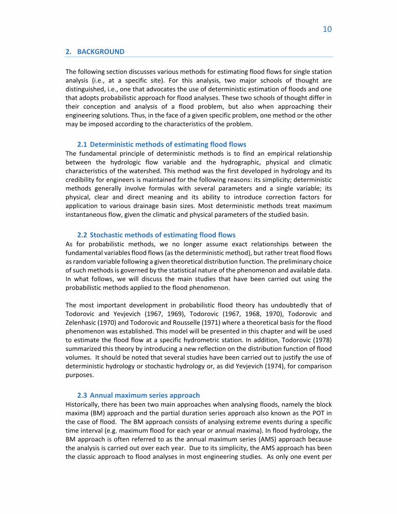
2. BACKGROUND 

 The following section discusses various methods for estimating flood flows for single station analysis  (i.e.,  at  a  specific  site).  For  this  analysis,  two  major  schools  of  thought  are distinguished, i.e., one that advocates the use of deterministic estimation of floods and one that adopts probabilistic approach for flood analyses. These two schools of thought differ in their  conception  and  analysis  of  a  flood  problem,  but  also  when  approaching  their engineering solutions. Thus, in the face of a given specific problem, one method or the other may be imposed according to the characteristics of the problem.  

2.1 Deterministic methods of estimating flood flows The  fundamental  principle  of  deterministic  methods  is  to  find  an  empirical  relationship between  the  hydrologic  flow  variable  and  the  hydrographic,  physical  and  climatic characteristics of the watershed. This method was the first developed in hydrology and its credibility for engineers is maintained for the following reasons: its simplicity; deterministic methods  generally  involve  formulas  with  several  parameters  and  a  single  variable;  its physical,  clear  and  direct  meaning  and  its  ability  to  introduce  correction  factors  for application  to  various  drainage  basin  sizes. Most  deterministic  methods  treat  maximum instantaneous flow, given the climatic and physical parameters of the studied basin.  

2.2 Stochastic methods of estimating flood flows As  for  probabilistic  methods,  we  no  longer  assume  exact  relationships  between  the fundamental variables flood flows (as the deterministic method), but rather treat flood flows as random variable following a given theoretical distribution function. The preliminary choice of such methods is governed by the statistical nature of the phenomenon and available data. In  what  follows,  we  will  discuss  the  main  studies  that  have  been  carried  out  using  the probabilistic methods applied to the flood phenomenon.  The  most  important  development  in  probabilistic  flood  theory  has  undoubtedly  that  of Todorovic  and  Yevjevich  (1967,  1969),  Todorovic  (1967,  1968,  1970),  Todorovic  and Zelenhasic (1970) and Todorovic and Rousselle (1971) where a theoretical basis for the flood phenomenon was established. This model will be presented in this chapter and will be used to estimate the flood flow at a specific hydrometric station.  In addition, Todorovic (1978) summarized this theory by introducing a new reflection on the distribution function of flood volumes.  It should be noted that several studies have been carried out to justify the use of deterministic hydrology or stochastic hydrology or, as did Yevjevich (1974), for comparison purposes.  

2.3 Annual maximum series approach Historically, there has been two main approaches when analysing floods, namely the block maxima (BM) approach and the partial duration series approach also known as the POT in the case of flood.  The BM approach consists of analysing extreme events during a specific time interval (e.g. maximum flood for each year or annual maxima). In flood hydrology, the BM approach is often referred to as the annual maximum series (AMS) approach because the analysis is carried out over each year.  Due to its simplicity, the AMS approach has been the classic approach to flood analyses in most engineering studies.  As only one event per 

  11  

year is considered with the AMS approach then these events are most likely  independent random variables.  Under the assumption that the annual floods are from a stationary time series, then a simple frequency distribution functions (Gumbel, lognormal, etc.) can be fitted to these floods and yield estimates of discharge for different frequencies.   

 

2.4 Annual maximum series distribution In  studies  characterizing  natural  flow  regimes,  environmental  flows  and  floods  in  New Brunswick (Aucoin et al. 2011; El‐Jabi et al. 2015), it was found that the GEV distribution was an  appropriate  distribution  to model  the  annual maximum  flows  at most  of  the  gauging stations in New Brunswick.   

2.5 Peak over threshold  Although the AMS approach is simple in application, it has the disadvantage of considering only  one  flood  per  year.    As  such,  the  sample  size  is  limited  to  the  number  of  years  of observation.   By considering only one flood per year,  it  is often observed that the annual flood during some years are relatively small in comparison to secondary floods of other years.  This means that this approach most likely considers data that should not be considered at floods  while  disregarding  important  flood  information.    Another  drawback  of  the  AMS approach is that it cannot analyse other important flood characteristics, such as flood volume or  flood duration as  this approach considers only  the magnitude of  floods.   To overcome these  limitations,  the  partial  duration  series  approach  can  be  used  instead  of  the  AMS approach.   The partial duration series approach consists of analysing all discharge above a specific threshold or truncation level that is selected to reflect only extremes events (e.g., floods). In the case of floods, the partial duration approach is often referred to as the Peak Over Threshold approach or POT.  One of challenge of the POT approach lies in the selection of  the  threshold  level.    If  the  truncation  level  is  set  too  high,  fewer  observations  are considered  in the analyses and the sample size can be  limited for  further analysis.    If  the truncation  level  is  set  too  low,  the  retained  flood  data  could  be  serially  correlated,  thus violating  the  independence  assumption.    As  the  POT  analyses  all  flows  above  a  certain truncation level (or threshold), and as such, flood characteristics (magnitude, duration and volume) can also be part of the analysis.  

2.6 Peak over threshold – Selection of threshold value Selection  of  threshold  values  remains  an  important  aspect  of  the  POT method,  however many methods exist  in  literature with no consensus of a better method. Earlier  research suggested selecting threshold values based on fixed values of mean number of exceedances per year while such as 1.15, between 1.2 and 2 or greater than 1.65 (Lang et al. 1999). Several graphical methods have been developed as well as tools for selecting threshold values. One method consists of plotting the ratio of the mean number of events over the variance of the number of events for different threshold values. The method, developed by El‐Jabi and al. (1986), utilizes an important property of the Poisson distribution; that the ratio of the mean and variance are equal to 1. This method is applied by selecting the threshold value for ratio of the mean and variance that are near 1 with the most data (e.g., Caissie and El‐Jabi 1991). Tanaka and Takara (2002), in a study of threshold selection methods, compared six graphical methods and found that the stability of the distribution parameters were good indicators of threshold values. Physical properties can also be used in the selection of threshold values.  

  12  

2.7 Peak over threshold – Occurrence distribution The distribution of the occurrence of floods differs from that of the exceedances as it is used to  describe  a  discrete  phenomenon.  The  Poisson  distribution  has  often  been  used  in frequency  analysis  to  describe  the  arrival  rate  of  floods  (Todorovic  and  Zelenhasic  1970, Ashkar and Rouselle 1983a, b, Caissie and El‐Jabi 1992). Cunnane (1979), in a study analysing arrival  rates  found  that  some  data  from  gauging  stations  did  not  follow  the  Poisson distribution and suggested the negative binomial distribution as an alternative. Önöz and Bayazit  (2001)  studied  three distributions  for  the  arrival  rates,  the Poisson, binomial  and negative  binomial  distributions.  It  was  found  that,  when  used  with  the  exponential distribution, results were near identical, regardless of the chosen occurrence distribution. A study by Bezak and al. (2014) comparing the AMS method to the POT method also found that the binomial distribution did not offer better results than with the Poisson distribution. 

 

2.7.1 Independence criteria Several  methods  have  proposed  to  eliminate  certain  floods  to  make  sure  floods  are independent when carrying a frequency analysis using the POT method. Lang et al. (1999) outline  the methods used  in  literature  to achieve  such  independence among  floods. One method suggests eliminating the smaller of two floods from the series based on the time between  events  and  the minimum discharge  between  events.  Another method  suggests eliminating  floods  based  on  the  time  to  peak  of  the  first  five  flood  peaks  deemed independent. Ashkar and Rouselle (1983b) suggest trying other measures to eliminate the independence  aspect  such  as  raising  the  threshold  level  prior  to  resorting  to  eliminating floods from the series. 

 

2.8 Peak over threshold – Exceedance distribution During the earlier stages of the POT method, the exponential distribution was used in many studies (Todorovic and Zelenhasic (1970), El‐Jabi and al. (1981), Ashkar and Rouselle (1983a), among  others). More  recent  studies  have  shown  that  the  use  of  the Generalized  Pareto distribution to describe the exceedance distribution is likely better base on the fact that is has one more parameter and therefore offering a greater flexibility (Ashkar et Ouarda 1996, Bhunya et al. 2013, Ben‐Zvi 2016, Gharib and al. 2017). 

 

2.9 Flood volume and duration When using the POT approach, floods are characterized, not only by their magnitude, but also by their associated volume and duration. Many examples in literature study bivariate or multivariate  analyses  to  describe  the  joint  characteristics  of  flood  phenomena  (Yue  and Rasmussen 2002, Assia and al. 2012, Bačová Mitková and Halmová 2014). However, few have considered univariate  analysis  of  flood  characteristics. Vukmirović  and Vukmirović  (2017) developed a method for univariate analysis to each flood characteristic (magnitude, volume and  duration).    In  the  present  study  both  flood  volume  and  flood  duration  will  also  be analyzed to better characterize flood within the province of New Brunswick.    

  13  

3. METHODOLOGY 

3.1 Flood frequency analysis A flood frequency analysis will be carried out using two different approaches, namely the 

AMS approach and the POT approach.  This section will provide details on the equations and 

methodology using to carry out the analyses.   

3.2 The GEV distribution function used in the AMS approach For the analysis of the AMS approach the GEV distribution is most often used in the analysis.  The cumulative distribution of the GEV is given by, 

  1/

  (1) 

 

where σ is the scale parameter,  is the location parameter and  is the shape parameter.  If we isolate x from equation (1), we have,  

  ln 1   (2) 

 

where x represents the discharge of different value of F(x).  

In hydrology, F(x) in equation (2) is also expressed as, 

 

  1   (3) 

 

where T represents the recurrence interval in years, such that a 2‐year event has a F(x) = 0.5 and a 100‐year event a F(x) = 0.99.  Therefore, the estimation of the discharge of different recurrence interval using the GEV distribution QT_GEV is given by, 

 

  _ ln 1 1   (4) 

 

Annual Flood Series were extracted from the data by isolating the largest peak discharge for 

each year of record. The scale, location and shape parameters for GEV distributions will be 

calculated  using  the  maximum  likelihood  method.  Using  equation  (3),  discharge  values 

corresponding to typical return periods (2‐, 5‐, 10‐, 20‐, 50‐ and 100‐years) were calculated 

for each station. Plots were then used to verify the fit of the GEV distribution with the annual 

maximum observations.  

 

  14  

3.3 Distribution of the occurrence of floods in the POT analysis The POT approach requires the study of two distinctive properties of floods, namely the time of  the  occurrence  of  floods  and  the  characteristics  of  floods  (magnitude,  duration  and volume).    Figure  1  illustrates  a  discharge  hydrograph  with  associated  POT  events  which describe flood exceedances above the truncation level (QR).  In this figure, every event above 

the truncation level is associated with a flood exceedance,  (magnitude), a flood duration and a flood volume where only the flood exceedances are represented in Figure 1b.  As such, 

flood exceedances, i  correspond to an event at specific  time (i). The distribution of  the number  of  exceedances (t)  in  a  time  interval  (0,t]  has  been  analyzed  in  many  studies (Todorovic and Zelenhasic 1970; Todorovic and Woolhiser 1972) and is generally observed to follow a Poisson distribution (Ashkar and Rousselle 1983a).  The time interval (0,t] for the analysis of floods is generally taken as the year, unless studies are carried out on a seasonal basis.  

 

 

Figure 1: Flow hydrograph with identification of flood characteristics 

 

In  the  case  where  the  number  of  exceedances  follow  a  Poisson  distribution,  then  the equation is given by,  

 

  !  (5) 

 

where n represents the number of events (exceedances) in a particular time interval (0,t] and 

 represents the parameter of Poisson distribution (i.e., the mean number of events within the time intervals (0,t]).  In equation (5), P(0) would represent the probability of having no event in the time interval whereas P(n) represents the probability of having n events.  The 

mean number of events in the time interval or  (the parameter of the Poisson distribution) is calculated by the following equation, 

  15  

 

          (6) 

 

One important property of the Poisson distribution is that the mean and the variance are equal, therefore the variance is given by, 

 

          (7) 

 

The ratio of equation (2) and (3) which gives a value of 1 is often used in studies to determine if the occurrence of flood follow a Poisson process. 

 

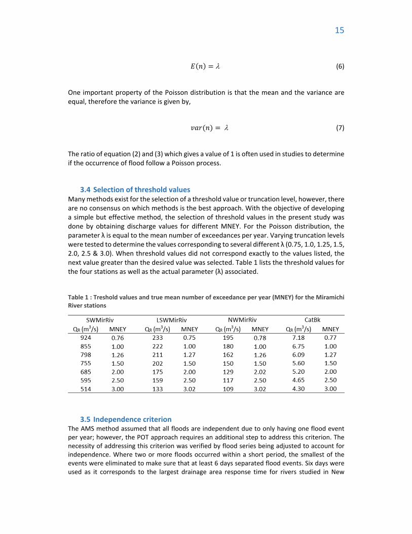
3.4 Selection of threshold values Many methods exist for the selection of a threshold value or truncation level, however, there are no consensus on which methods is the best approach. With the objective of developing a simple but effective method, the selection of threshold values  in the present study was done  by  obtaining  discharge  values  for  different MNEY.  For  the  Poisson distribution,  the parameter λ is equal to the mean number of exceedances per year. Varying truncation levels were tested to determine the values corresponding to several different λ (0.75, 1.0, 1.25, 1.5, 2.0, 2.5 & 3.0). When threshold values did not correspond exactly to the values listed, the next value greater than the desired value was selected. Table 1 lists the threshold values for the four stations as well as the actual parameter (λ) associated. 

 

Table 1 : Treshold values and true mean number of exceedance per year (MNEY) for the Miramichi River stations 

 

 

3.5 Independence criterion The AMS method assumed that all floods are independent due to only having one flood event per year; however, the POT approach requires an additional step to address this criterion. The necessity of addressing this criterion was verified by flood series being adjusted to account for independence. Where two or more  floods occurred within a short period,  the smallest of  the events were eliminated to make sure that at least 6 days separated flood events. Six days were used  as  it  corresponds  to  the  largest  drainage  area  response  time  for  rivers  studied  in  New 

  16  

Brunswick.   The  response  time equations were obtained  from Gray  (1970).   Only  the POT‐GP model was used for this purpose.  

 

3.6 Distribution of the magnitude of flood exceedances Once that the distribution of the occurrence of floods/exceedances is properly determined then the distribution of both the exceedances and the maximum exceedances is of interest.  The distribution of  the maximum or annual exceedances  is given by  following cumulative distribution function, F(x) (Todorovic and Zelenhasic 1970; Zelenhasic 1970): 

 

  ∑   (13) 

 

where H(x) is the cumulative distribution of the exceedances (e.g., exponential, Generalized Pareto or other distributions) and where P(n) represents the distribution of the occurrence of event as described above (Poisson or negative binomial distribution).   In equation (13), there  is  no  restriction  on  the  distribution  of  the  occurrence  of  floods;  however,  if  the occurrence of  floods  is a Poisson process,  then substituting equation  (5)  into  (13)  can be further simplified to the following equation, 

 

    (14) 

 

where  is the Poisson parameter and H(x) represents the distribution of exceedances.  One of  the  simplest distributions of H(x), which has been widely used  in  flood analysis,  is  the exponential  distribution  (Todorovic  and  Zelenhasic  1970;  Todorivic  and  Rousselle  1971; Caissie and El‐Jabi 1991).  As such, H(x) has the following equation: 

 

  1   (15) 

 

where,   is the exponential distribution parameter and can be calculated using the following equation: 

 

    (16) 

 

Therefore, the cumulative distribution for the POT model equation (14) is given by: 

 

    (17) 

or 

    (18) 

  17  

 

Equation (18) represent the classic double exponential function which has been used in flood analysis and very similar to the Gumbel model when considering floods as AMS.   We can extract x from equation (18) to calculate exceedances as a function of different frequencies F(x) as,  

 

 

  (19) 

where x represents the exceedances of different frequencies, and all other parameters have been defined previously.  Therefore, the discharge for different recurrence intervals when introducing equation (3) in equation (19) and then adding the truncation level QR is given by, 

  _   (20) 

where QT_Exp  represents  the discharge of different  recurrence  intervals by  the POT model using the exponential distribution. 

 

Similarly,  we  can  analyses  exceedances  following  a  GP  distribution  rather  than  the exponential  distribution.    The  GP  distribution  when  used  in  POT  model  is  given  by  the following equations: 

 

  1 1   (21) 

 

In equation (21),   is the scale parameter and κ is the shape parameter, which are calculated by  the  maximum  likelihood  estimate  method.    Therefore,  if  we  use  the  GP  distribution instead of  the  exponential  distribution  in  the POT model,  the  general  equation becomes when the occurrence of flood follows a Poisson process,  

 

    (22) 

 

which is the same as equation (14) and therefore the distribution of annual maxima is given by, 

 

 

  (23) 

 

and we can simplify equation (23) to,  

  18  

 

  (24) 

similar to the exponential distribution, we can extract x from equation (24) giving,  

 

 

1   (25) 

 

where x represents the exceedance of different recurrence intervals for the POT model when using the GP distribution.  The discharge of different recurrence intervals is given by equation (25) by adding the truncation level (QR) and substituting F(x) in equation (25) by equation (3), 

 

   _

1   (26) 

 

Having established threshold values  for corresponding MNEY,  flood series were extracted from the data by isolating all peak values above the thresholds. Using equations (20) and (26) for  the POT‐Exp and POT‐GPD  respectively, discharge values were determined  for  typical recurrence intervals. The results were then plot on Gumbel paper to illustrate the fit with the observed annual maximum values. 

 

3.7 Distribution of flood volumes and durations The exponential and GP distributions were used to fit volume and duration data. In the case of  univariate  analysis,  the  same  development  that  is  done  with  the  magnitude  of exceedances. In the case of exceedance magnitude, discharge for different return periods is given by  equation  (20)  and  (26)  for  the  POT‐Exp  and POT‐GP models  respectively.  These equations are quite similar to equations (19) and (25), respectively, where the sole difference is  the  addition  of  the  base  flow  to  the  calculated  exceedance  discharge.  In  the  case  of exceedance  volume and exceedance duration,  no base  value  is  added.  Thus,  exceedance volumes for different return periods are given by, 

 

  _   (20) 

for the exponential distribution, where VT_Exp is the exceedance volume for different return periods,  is the Poisson distribution parameter, T is the return period and  , the exponential distribution parameter, is given by, 

                                    (16) 

and  

  19  

  _

1   (26) 

for the Generalized Pareto distribution where VT_GP is the exceedance volume for different return periods  is the Poisson distribution parameter, T is the return period,   is the scale parameter and κ is the shape parameter. 

 

In the case of exceedance durations for different return periods, they are given by, 

 

  _   (20) 

for the exponential distribution, where DT_Exp is the exceedance duration for different return periods,  is the Poisson distribution parameter, T is the return period and  , the exponential distribution parameter, is given by, 

                                    (16) 

and  

  _

1   (26) 

for the Generalized Pareto distribution where DT_GP is the exceedance duration for different return periods,  is the Poisson distribution parameter, T  is the return period,   and κ are the scale parameter and the shape parameter respectively.  

From the flood series used in the POT‐GPD and POT‐Exp magnitude analysis, volume and duration data were extracted. The duration of flood events corresponds to the amount of days for which the discharge level was greater than the truncation level. Flood volumes represent the quantity of water above the truncation level. The fitted distribution was verified with the annual maximum 

observations for the volume and duration for MNEY of 1.  

Flood  volumes  and  durations  were  also  analysed  on  a  per  decade  basis.  Where  partial decades occurred, values were adjusted to account for the differences in years. 

 

All the above calculations were carried out using R scripts (R Development Core Team 2015) where different distributions were programed and subsequently analysed. 

 

 

   

  20  

4. STUDY AREA AND DATA 

 

4.1 Choice of hydrometric stations and detailed analysis of streamflow data In  the  development  of  this  project,  the  selection  of  hydrometric  stations  used  for  the calculations of flood flow characteristics largely depends on the quality of the data.  As such, stations will be selected based on previous studies and best currently available data. This task is essential for the preparation data for phase II of the project.  Stations should have enough  years  of  records  to  ensure  the  representativeness  of  the  various  hydrological regimes within the province, meetings will be conducted between the Department of the Environment and Local Government and Environment Canada and the selected station will be discussed.   

The importance of hydrometric gauging station networks for surface water monitoring is well established, given the usefulness of collected hydrometric data for decision‐making related to water resources management. Although, many water resource decisions, project designs and project management  rely  on  information  gained by hydrometric  gauging  stations.  In other  words,  short‐comings  in  a  gauging  network  can  lead  to  greater  hydrological uncertainty, which can lead to inefficient project design and resource management, which in turn can have diverse consequences. For example, uncertainty can lead to over‐designing, which adds unnecessary extra project costs. In addition, under designing is also possible, this could lead to project failure and extra costs as well, including the potential lost of human’s life. Poor resource management can also impact the population as well as the environment.  

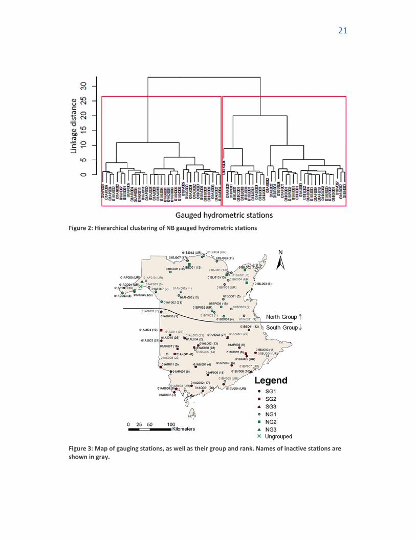
The  present  study  proceeded  by  first  dividing  New  Brunswick  into  two  groups,  using  a clustering analysis based on high flow timing and latitude. This had the effect of creating a north‐south group.  Two clusters were formed in the hierarchical clustering analysis, based on  high  flow  timing.  The  attributes  from  which  similarities  will  be  defined  need  to  be specified  for  clustering  analysis  (Burn  and  Goulter  1991).  Once  this  is  done,  clusters  are formed by grouping similar observations together in such a way that variance is minimized within a cluster and maximized between clusters (Khalil and Ouarda 2009). The division of the  complete  network  into  clusters was  done  using  hierarchical  agglomerative  clustering (based on Euclidean distance), accomplished using R software toolbox (R Development Core Team 2015). In this type of clustering, each individual station is initially considered as being its own cluster. Afterwards, an iterative process is used in which only the two most similar clusters  (least  Euclidean  distance  between  two  clusters  of  all  possible  combinations)  are joined together to form one new cluster per iteration. This is repeated until a single cluster remains,  containing  all  the  individuals.  In  this  study,  two  attributes  were  used  for  the clustering analysis: latitude of each station, and high flow timing. The latter was computed as  the  30‐day  period  with  the  highest  mean  flow  (moving  average).  The  two  attributes (latitude  and  timing)  were  chosen  with  the  purpose  of  dividing  the  province  based  on climate. The high flow timing is typically dependent on temperature, due to snowmelt. The northern  part  of  the  province  is  typically  cooler  than  the  southern  part.  As  such,  using latitude and high flow timing,  it  is expected that the province will be divided into clusters based on both geographical location and hydro‐climatological processes. A dendrogram was obtained  using  the  hierarchical  clustering  technique  (Figure  2)  where  station  number identifies each site (Figure 3). The two major groups formed by the clustering analysis can be seen on this figure (identified in red). All 67 stations identified by Environment Canada were used in this analysis. 

  21  

 

 

 

Figure 2: Hierarchical clustering of NB gauged hydrometric stations 

 

 

Figure 3: Map of gauging stations, as well as their group and rank. Names of inactive stations are shown in gray. 

 

  22  

4.2 Application of the POT model on hydrometric stations in the Miramichi River system 

The Miramichi River is located near the central‐eastern part of New Brunswick and empties into  the Gulf of  St.  Lawrence.  The Miramichi watershed  covers  about one‐quarter of  the Province of New Brunswick and measures 190 km from east to west and 95 km from north to south (Chiasson 1995). It covers 13,000 km2 including 300 km2 of estuary. The meander of the Miramichi River  is approximately 250 km long. The network of this river  includes two main branches which are the Southwest Miramichi River and the Northwest Miramichi River.  Most of the territory consists of unpopulated forests. The territory has few large lakes but many small lakes (Chiasson, 1995). Forests supply the timber industry either for lumber or the  paper  industry.  In  the  north,  until  2000  there  were  mines  of  zinc,  copper  and  lead (http://www.mreac.org/watershed.html). 

 

4.3 Climate 

The climate of the Miramichi River watershed is considered more continental than maritime. The average temperature is 4.3 ° C. The month of January has the coldest monthly average air temperature at ‐11.8 ° C and the hottest July average at 18.8 ° C (Caissie et al., 1995c). Mean maximum water temperatures of 18 to 22 ° C are reached in July and August and then drop rapidly to near 0 ° C in December (Chiasson, 1995). 

There is an average of 160 days of precipitation per year. The mean annual precipitation is on average between 860 mm and 1365 mm. The annual long‐term average is estimated at 1 130 mm per year (Caissie et al., 1995c). The driest months are those from April to June and the maximum rainfall is in November. However, the Miramichi does not show large variations in its monthly precipitation, as the monthly average is close to 100 mm per month. 

 

4.4 Hydrology 

The flow of the Miramichi River at the mouth varies from less than 25 m3/s to more than 6,000 m3/s. The average annual flow for the entire Miramichi River watershed is between 306 m3/s and 317 m3/s at the mouth. The median flow rate is 158 m3/s (Caissie and El‐Jabi, 1995). 

The average annual discharge is about 63% of precipitation (714 mm / year). This means that about 37% of the rainfall is consumed by the plants or stored in the subsoil, i.e., loss through evapotranspiration. The median flow is equivalent to half the median flow and is 357 mm / year. The highest flows are observed during the months of April and May and are generated by  snowmelt.  There  is  also  a  second‐high  flow  period which  occurs  generally  during  the month of November. High flow months reach values 6 times that of the average annual flow. The winter months (January to March) and summer months (August to September) are those with the lowest monthly flows, during these periods the flow level can be less than 10% of the mean annual flow. 

Mean annual runoff values for the Miramichi River are comparable to other areas of New Brunswick except for the Fundy region. In addition, New Brunswick's smaller rivers generally have more severe low water conditions than the Miramichi. 

  23  

The study of extreme events is important because they play important roles for hydrological regime, water management and fisheries. The Caissie and El‐Jabi  (1995) evaluated the bi‐annual flood for the entire Miramichi watershed at 16.3 mm, or 0.189 m3/s per km2 for a watershed. The floods of 5, 25, 50 and 100 years correspond respectively to 1.5, 2, 2.5 and 3 times  the  biennial  flood.  The  2‐year  low  flow  was  also  determined  at  0.24  mm  for  the Miramichi  watershed,  or  0.0028  m3/s  per  km2  for  a  basin.  The  low  water  flow  with  a recurrence of more than two years is expressed in relation to a factor of the two‐year low water  flow.  The  10,  25,  and  50‐year  low  water  flow  corresponds  to  1/2,  1/3,  and  1/5, respectively, of the biennial low flow. 

 

4.5 Hydrometric stations 

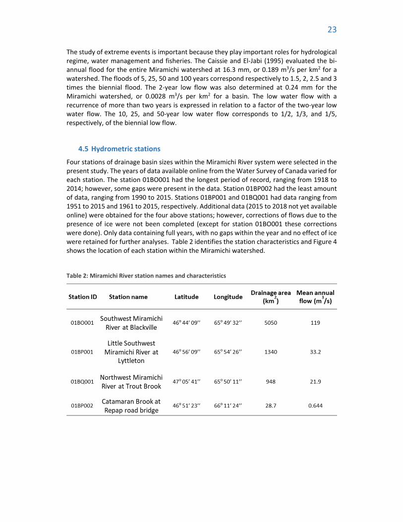
Four stations of drainage basin sizes within the Miramichi River system were selected in the present study. The years of data available online from the Water Survey of Canada varied for each station. The station 01BO001 had the longest period of record, ranging from 1918 to 2014; however, some gaps were present in the data. Station 01BP002 had the least amount of data, ranging from 1990 to 2015. Stations 01BP001 and 01BQ001 had data ranging from 1951 to 2015 and 1961 to 2015, respectively. Additional data (2015 to 2018 not yet available online) were obtained for the four above stations; however, corrections of flows due to the presence of  ice were not been  completed  (except  for  station 01BO001  these  corrections were done). Only data containing full years, with no gaps within the year and no effect of ice were retained for further analyses.  Table 2 identifies the station characteristics and Figure 4 shows the location of each station within the Miramichi watershed. 

 

Table 2: Miramichi River station names and characteristics 

 

 

  24  

 

Figure  4:  Miramichi  watershed  with  location  of  hydrometric  stations  (black  dot)  and  assigned catchment area (colored areas) 

 

 

 

 

 

 

 

 

 

 

 

 

  25  

5. RESULTS AND DISCUSSIONS 

 

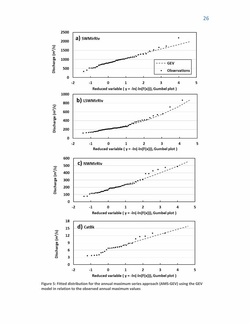
5.1 AMS Flood magnitude The AMS‐GEV model, as well as the POT‐GPD and POT‐Exp models were used to determine discharge values for different recurrence intervals (also known as return periods). Table 3 presents the calculated discharge values for 2‐, 5‐, 10‐, 20‐, 50‐ and 100‐years return periods with the AMS‐GEV model as well as the location, scale and shape parameters. The range of values between  the 2‐ and 100‐year  flood varies  in proportion  to  the drainage area. The Southwest Miramichi River (SWMirRiv) station, which has the largest drainage area, had the largest range in values, from 892 m3/s for the 2‐year flood and 1974 m3/s for the 100‐year flood. The Little Southwest Miramichi River (LSWMirRiv) and the Northwest Miramichi River (NWMirRiv) showed flows of between 231‐874 m3/s and 191‐555 m3/s, respectively.   The CatBk station had the smallest range in values, from 6.9 m3/s for the 2‐year flood and 15.9 m3/s for the 100‐year flood.  

 

        Table 3: Calculated discharge (m3/s) for different return periods using the AMS‐GEV model 

 

 

Figure 5 shows the fit of the AMS‐GEV model with the observed annual maximum values at each station. A good fit was observed between the data and the fitted values for the four stations.  For all stations, a slight departure between the observed and the fitted values was observed at higher flows. 

 

5.2 POT Flood magnitude Table 4 shows the calculated discharge values for different return periods and for varying values of MNEY for the POT‐GPD model as well as the distributions’ parameters. Results show a variation in calculated values for different MNEY at each station. Variability was observed to be lower at low return floods (e.g., 2‐year) and slightly higher for high return floods (e.g., 100‐year).  Results  are  relatively  very  similar  to  those  found using  the AMS‐GEV method. Most GP shape parameter values obtained for different return periods and different MNEY were positive or near zero except for the exception of the CatBk which had four negative shape parameters for MNEY of 0.75, 1.00, 1.25, and 1.50, ranging from ‐0.676 and ‐0.260, while the other three shape parameters at that station were near zero. 

  26  

 

Figure 5: Fitted distribution for the annual maximum series approach (AMS‐GEV) using the GEV model in relation to the observed annual maximum values 

  27  

Table 4: Calculated discharge (m3/s) for varying mean number of exceedances per year for different return periods using the POT‐GP model 

 

  28  

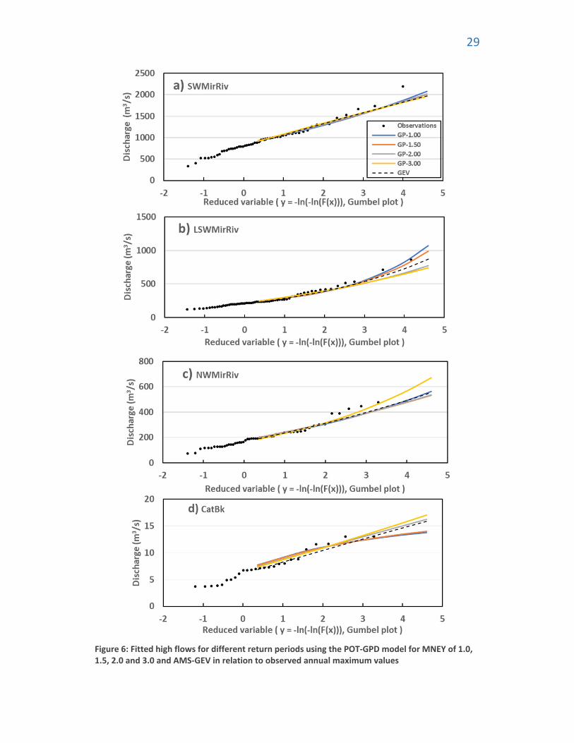
Figure 6 shows the fit of the POT‐GPD model with the annual maximum observations as well as a comparison with the AMS‐GEV fitted distribution (dashed line). As with the AMS‐GEV model, a good fit was found between calculated values with the POT‐GPD and the annual maximum observations. Values remained generally similar between the AMS‐GEV and the POT‐GPD for different return periods. However, the CatBk, which has the smallest drainage area, showed slightly higher calculated discharges for low return floods. The impact of the negative shape parameter for CatBk can be noticed in Figure 6d.  

 

Calculated discharge values for different return periods and for varying values of MNEY and the  corresponding  exponential  parameter  (1/β)  for  the  POT‐Exp model  are  presented  in Table 5. Similar to the POT‐GPD model, results vary based on the MNEY with the greatest variations observed for large return periods. 

 

Figure 7 shows the fit of the POT‐Exp model with the annual maximum observations as well as a comparison with the AMS‐GEV curve (dash line). The POT‐Exp model did not fit the data as well as the POT‐GPD model, especially for high return floods. The fit for low return periods was  relatively  good,  however,  the  POT‐Exp  did  not  fit  well  the  data  for  the  LSWMirRiv. Calculated discharges with the POT‐Exp model were significantly lower than those calculated with the AMS‐GEV for high return periods. It should be noted that the AMS‐GEV model, was already lower than 5 out of the 6 largest observations for LSWMirRiv. 

 

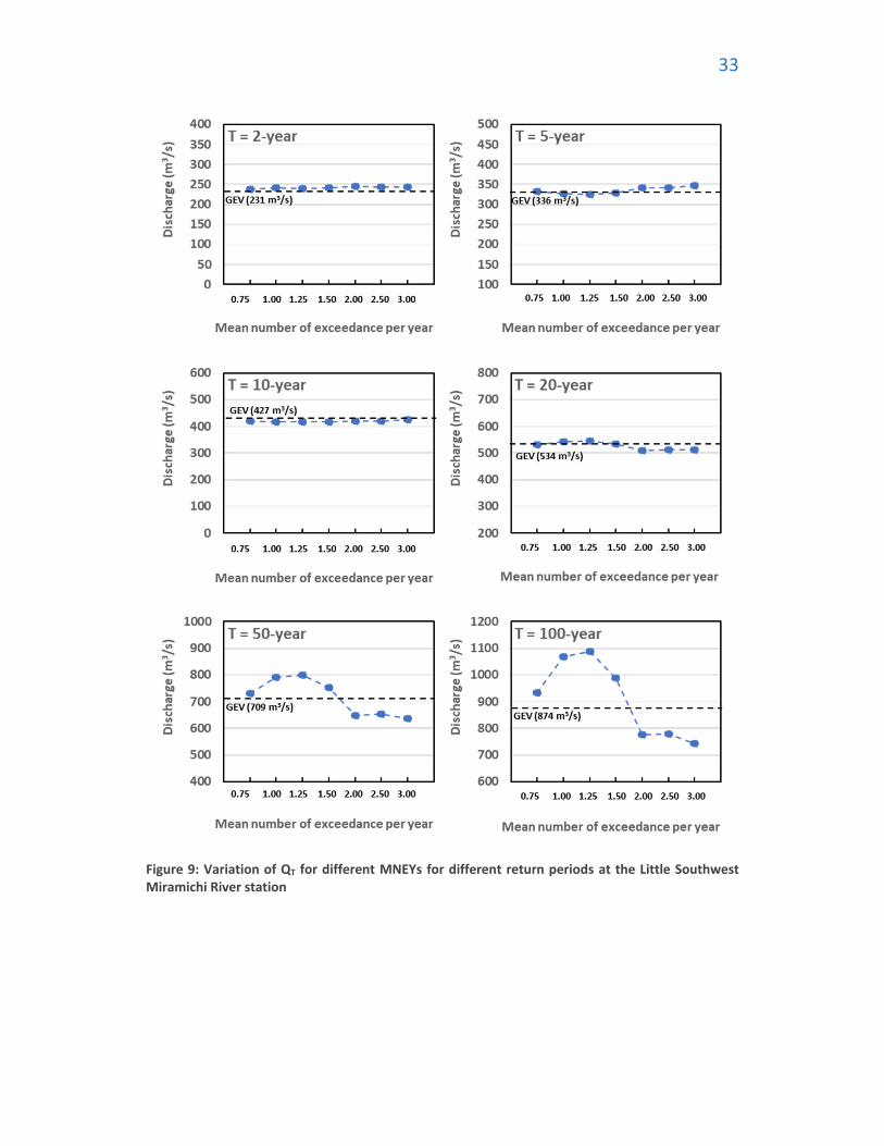
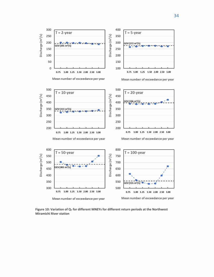
Figures 8 to 11 show the calculated discharge values for different return periods with the POT‐GPD model as a function of the mean number of events per year (MNEY). The calculated AMS‐GEV value are also presented on these figures for comparison purposes. These figures highlight  that  no  systematic  trend  exists  between  the  MNEY  and  flows  for  different recurrence intervals.  For low return floods, very little variability was observed as a function of  increasing MNEY.   This was most noticeable  for  the LSWMirRiv where flows were very similar for different MNEYs and very comparable to those of the GEV model (Figure 8). The greatest  variability  was  observed  at  high  return  floods,  but  no  consistent  trends  were observed. 

 

  29  

 

Figure 6: Fitted high flows for different return periods using the POT‐GPD model for MNEY of 1.0, 1.5, 2.0 and 3.0 and AMS‐GEV in relation to observed annual maximum values 

  30  

Table  5:  Calculated  discharge  in  (m3/s)  for  varying  mean  number  of  exceedances  per  year  for different return periods using the POT‐Exp model 

 

  31  

 

Figure 7: Fitted high flows for different return period using the POT‐Exp model for MNEY of 1.0, 1.5, 2.0 and 3.0 and AMS‐GEV in relation to observed annual maximum values 

  32  

 

Figure 8: Variation of QT for different MNEYs for different return periods at the Southwest Miramichi River station 

 

  33  

 

Figure 9: Variation of QT for different MNEYs for different return periods at the Little Southwest Miramichi River station 

  34  

 

Figure 10: Variation of QT for different MNEYs for different return periods at the Northwest Miramichi River station 

 

 

  35  

 

Figure 11: Variation of QT for different MNEYs for different return periods at the Catamaran Brook station 

 

 

 

  36  

5.3 Independence criterion The necessity of considering  the  independence of  flood exceedances  in the POT model  is important, especially when the MNEY becomes high (where floods could be close together and potentially correlated).  As described in the method section, an independence criterion was applied within the present study where the smallest flood was deleted when two floods were separated by less than 6 days.  A comparison was made between quantile discharges calculated from flood series when the independence criterion was (deletion of floods) and was not applied. The POT‐GPD model was used for this analysis. Figure 12 shows the results of this analysis, as expressed as a difference in percentage between the quantile discharges with and without an applied criterion. Differences were relatively low with only two values greater  than  4%.  The  highest  differences  were  found  to  be  for  the  100‐year  quantile discharge at the LSWMirRiv and NWMirRiv at 5.4% and 5.5% respectively. Again, no trends were observed as a function of MNEY and different return period.  In general, it was observed that  very  few  events  were  observed  to  less  than  6  days  apart  and  thus  the  resulting calculated discharge for different return period was not affected considerably (less than 4%). 

  37  

 

Figure 12: Difference in calculated QT when applying a 6‐day interarrival independence criterion (see text for details) 

  38  

5.4 Flood volume Using the POT approach, flood volumes were determined at each station for several MNEYs. It should be noted that for all the analysis comparing stations in terms of volume, the specific volume  (volume  per  unit  area;  expressed  in  mm)  was  used.  This  was  done  to  remove drainage area as an overwhelmingly dominant variable when it comes to explaining volumes.  

 

Figure 13 shows the average yearly flood volume per surface area (expressed in mm) for each 

station for different MNEYs. As expected, the higher the MNEYs (which represents a lower 

truncation level), a larger flood volume was observed. This figure shows that flood volumes 

are  relatively  similar  among  rivers,  regardless  of  drainage  area.   When  considering  small 

MNEY values (0.75 & 1), similar values were observed.  However, a greater difference was 

observed  for  larger  MNEYs  (2.5  &  3)  where  CatBk  showed  slightly  lower  flood  volume 

compared to other stations. 

 

Figure 23: Average specific flood volume per year for different MNEYs 

 

The GP and exponential distributions were also fitted to the flood volumes for a MNEY of 1. Figure 14 shows the results for the fit of the GP and Exp distributions along with the annual maximum  flow  volumes  for  the  four  stations.  Both  distributions  fitted  the  flood  volume observations  well.  However,  for  the  LSWMirRiv,  the  GP  distribution  showed  an overestimation of flood volumes for large return periods, while the exponential, even with a better fit, would underestimate the volume for high return period.  

Flood volumes were separated by decade for four different values of MNEY (1.0, 1.5, 2.0 and 3.0). Figure 15 presents the total volume per decade, in mm, for the four values of MNEY. Although results show high and low flow decades, no apparent trends of flood volumes over decades were observed.   It can be observed that the 1970s had slightly higher values and comparable to 2010s (NWMirRiv; Figure 15c), whilst the 1980s showed the lowest values. No apparent trends were observed, neither positive or negative, as a function of decades and as a function of the MNEY.  Figure 16 show the total flood volume by decades for the different stations for MNEY of 1 to compare among stations.  No apparent trends were observed over the years; however, the 1970s showed slightly higher values for the LSWMirRiv. 

  39  

 

Figure 34: Fit of calculated flood volume distribution to annual maximum volume observations for POT‐GP‐1 and POT‐Exp‐1 

  40  

 

 

                Figure 45: Total flood volumes per decade for MNEYs of 1, 1.5, 2 and 3 

 

  41  

 

 

 

 

 

             Figure 56: Total flood volumes per decade for MNEY of 1 

 

 

5.5 Flood duration Flood durations were determined at each station using the POT approach and for several MNEYs. The average duration of flood events is presented in Table 6. Flood durations were relatively  similar between stations except  for CatBk, where  flood durations were smaller, presumably due to the smaller drainage basin. For a mean number of exceedances per year of 1, station LSWMirRiv had only 2 out of the 26 identified events that had a flood duration greater than 1 day. 

                        Table 6: Average duration (days) per flood event for different MNEYs 

 

  Note:  = MNEY (mean number of events per year) 

 

Figure  17  compares  the  average  yearly  duration  for  which  discharge  levels  were  above truncation  levels  for  varying  values  of  MNEYs  at  each  station.  Durations  remain  similar 

  42  

between  the  three  stations  (with  the  largest  drainage  area;  SWMirRiv,  LSWMirRiv  and NWMirRiv) where CatBk showed slightly  lower duration values (e.g., generally  less than 4 days/year).  The duration of events increased with increasing MNEY. 

 

                 Figure 17: Average yearly duration of floods for varying MNEY 

Flood duration observations were also fitted to the GPD and exponential distributions for a MNEY  of  1.  Figure  18  shows  the  fitted  GP  and  exponential  distributions  with  the corresponding annual maximum flood durations. The GPD had a good fit for the duration and described  the  phenomenon  well  at  the  three  stations  with  large  drainage  areas.  The exponential distribution had a good fit  for small return periods, however, the distribution overestimated durations for floods of large return periods.  

Flood durations were also separated per decade for four mean number of exceedances per year (1, 1.5, 2 and 3). Figure 19 presents the total duration above threshold value per decade.  As with volume, no apparent trends appeared in the duration of floods over time. 

 

  43  

 

Figure 68: Fit of calculated flood duration distribution to annual maximum duration observations for POT‐GP‐1 and POT‐Exp‐ 

  44  

 

Figure 79: Total flood durations per decade for MNEYs of 1, 1.5, 2 and 3 

  45  

Figure 20 shows the total duration per decade for a MNEY of 1 at the four stations of the Miramichi River. Interestingly, for the SWMirRiv station, the duration of floods in 1980 was nearly doubled that of 1960, 15 and 9 days (adjusted value) respectively, however, specific flood volumes for those same decades remained relatively similar at 23.8mm and 20.5mm respectively.  

 

 

                Figure 8: Total flood duration per decade for a MNEY of 1 

 

 

 

 

 

 

 

 

 

 

 

 

 

  46  

6. CONCLUSIONS 

The purpose of this report was to outline the result obtained in phase I of the project. Phase 

I  included  the  identification  and  selection  of  hydrometric  stations  to  be  used  during  the 

province wide  analysis;  the  development  of  R  scripts/software  for  the  application  of  the 

AMS_GEV model, the POT_Exp and the POT_GP models to flood series’; the application of 

the  models  to  four  stations  within  the  Miramichi  River  basin;  and  determining  flood 

frequency characteristics (including the magnitude, the volume and the duration for several 

mean number of exceedances per year).  

For the province wide analysis, 67 hydrometric stations with drainage areas and mean flows 

varying from 3.89 km2 to 21 900 km2 and 0.1 m3/s to 420.1 m3/s respectively were identified 

and selected for further analyses. R scripts/softwares were developed to apply both models 

and  obtain  flood  characteristics.  The  R  scripts/software  were  used  for  the  fitting  and 

obtaining parameters of the GEV distribution in the case of the AMS model and for the fitting 

and obtaining parameters of the GP and Exp distributions to the POT model exceedances. 

Furthermore, durations of floods and the corresponding volumes were extracted in the case 

of the POT models. 

Several flood characteristics were obtained for four stations of the Miramichi River basin. 

Discharge  estimates  were  obtained  using  the  AMS  model  and  using  the  POT_Exp  and 

POT_GP models for several values of mean number of exceedances per year (MNEY). Results 

showed that the choice of the truncation level or the MNEY does impact slightly some of the 

results (flood flow) but more so for the duration and flood volume. 

Flood durations and volumes were determined using the POT approach to which GP and Exp 

distributions were  fit.  Flood durations  and  volumes were also presented by decades  and 

compared  between  different  mean  number  of  exceedances  per  year.  In  both  cases,  no 

significant trends were detected.  

For  the  POT  models,  discharge  values  were  obtained  with  flood  series  with  an  applied 

independence criterion of 6 days and without an applied criterion. Results suggest that the 

application of an independence criterion does not significantly impact the discharge values 

obtained.  In  fact, variability  in discharge values were greater between results obtain with 

different MNEY than with an independence criterion applied.  

 

 

 

 

 

 

 

  47  

AKNOWLEDGEMENTS 

This study was funded by the New Brunswick Environmental Trust Fund. The authors remain thankful to Darryl Pupek and Jasmin Boisvert at the Department of Environment and local government of New Brunswick for their helpful comments.                                           

  48  

REFERENCES 

Aissia M.‐A. B. et al., 2012. “Multivariate analysis of flood characteristics in a climate change context of the watershed of the Baskatong reservoir, Province of Québec, Canada,” Hydrological Processes, vol. 26, no. 1, pp. 130–142,   Ashkar F. and Ouarda T. B. M. J., 1996. “On some methods of fitting the generalized Pareto distribution,” Journal of Hydrology, vol. 177, no. 1–2, pp. 117–141, Mar.   Ashkar F.  and Rousselle J., 1983. “Some remarks on the truncation used in partial flood series models,” Water Resources Research, vol. 19, no. 2, pp. 477–480,   Ashkar F.  and Rousselle J., 1983. “The effect of certain restrictions imposed on the interarrival times of flood events on the Poisson distribution used for modeling flood counts,” Water Resources Research, vol. 19, no. 2, pp. 481–485,   Aucoin, F., D. Caissie, N. El‐Jabi and N. Turkkan, 2011. Flood frequency analyses for New Brunswick rivers. Can. Tech. Rep. Fish. Aquat. Sci. 2920: xi + 77p.   

Bačová Mitková V. and Halmová, D. 2014. “Joint modeling of flood peak discharges, volume and duration: a case study of the Danube River in Bratislava,” Journal of Hydrology and Hydromechanics, vol. 62, no. 3, pp. 186–196.  Ben‐Zvi, A. 2016. “Selecting series size where the generalized Pareto distribution best fits,” Journal of Hydrology, vol. 541, pp. 778–786.  Bezak, N. Brilly, M.  and Šraj, M. 2014.  “Comparison between the peaks‐over‐threshold method and the annual maximum method for flood frequency analysis,” Hydrological Sciences Journal, vol. 59, no. 5, pp. 959–977.   Bhunya, P. K.  Berndtsson, R. Jain, S. K.  and Kumar, R. 2013. “Flood analysis using negative binomial and Generalized Pareto models in partial duration series (PDS),” Journal of Hydrology, vol. 497, pp. 121–132.   Burrell,B. and Keefe, J. 1989. “Flood risk mapping in New Brunswick: A decade review” Canadian Water Resources Journal, vol. 14, no. 1, pp. 66‐77.   Caissie D. and El‐Jabi, N.  1992. “A stochastic study of floods in Canada: truncation level by region,” Canadian Journal of Civil Engineering, vol. 18, no. 2, pp. 328–330.   Caissie, D., & El‐Jabi, N. (1995). Hydrology of the Miramichi River drainage basin. Canadian special publication of Fisheries and Aquatic Sciences, 83‐96.  Cunnane, C. 1979. “A note on the Poisson assumption in partial duration series models,” Water Resources Research, vol. 15, no. 2, pp. 489–494.   El‐Jabi, N.  Ashkar, F. and Rousselle, J. 1981. “Estimations probabiliste et statistique des crues et de leurs parametres,” EP81‐R‐31RAPPORT GREMU 81/04 p. 114. École polytechnique de Montréal 

  49  

  El‐Jabi, N., Ashkar, F., Rousselle, J., and Hoang, V.D. 1986. Étude stochastique des crues au Québec. Ministère de l’Environnement, Québec, Direction des relevés aquatiques, H.P.‐59.  Ei‐Jabi, N., Turkkan, N. and Caissie. D.  2015. Characterisation of natural flow regimes and environmental flows evaluation in new Brunswick. Presented to the New Brunswick Environmental Trust Fund, Univertsité de Moncton, 168 p.  Fisher, R.A. and Tippett, L.H.C., 1928. Limiting Forms of the Frequency Distribution of the Largest or Smallest Member of a Sample, Proc. Cambridge Phil. Soc., vol. 24, no 2, pp. 180‐190.  Gharib, A. Davies, E.  Goss, G.  and Faramarzi, M. 2017. “Assessment of the Combined Effects of Threshold Selection and Parameter Estimation of Generalized Pareto Distribution with Applications to Flood Frequency Analysis,” Water, vol. 9, no. 9, p. 692.   Gray, D.M. 1970. Handbook of the principle of hydrology. NRCC, 13 chapters.  Karim, F. Hasan, M.  and Marvanek, S.  2017. “Evaluating Annual Maximum and Partial Duration Series for Estimating Frequency of Small Magnitude Floods,” Water, vol. 9, no. 7, p. 481.  Lang, M., Ouarda, T. B. M. J., & Bobée, B. 1999. Towards operational guidelines for over‐threshold modeling. Journal of Hydrology, 225(3–4), 103–117. https://doi.org/10.1016/S0022‐1694(99)00167‐5  Onoz B. et Bayazit M.  2001 “Effect of the occurrence process of the peaks over threshold on the flood estimates Journal of Hydrology,244, 1–2, 86‐96.  Tanaka S.  and Takara, K. 2002 “A study on threshold selection in POT analysis of extreme floods,” IAHS Publ. no. 271.299‐304.  Tiercelin, J.R., .1973. Modèles probabilistes en hydrologie, La Houille Blanche, no 7, pp. 547‐552.  Todorovic, P., 1967. A Stochastic Process of Monotonous Sample Functions, Math. Inst. of the Republic of Serbia, vol. 4, no 19, pp. 149‐158.  Todorovic, P., 1968. A Mathematical Study of Precipitation Phenomena, Report no CET67 – 68PT65, Colorado State Univ., 123 p.  Todorovic, P., 1970. On Some Problems  Involving Random Number of Random Variables, Ann. Math. Statist., vol. 41, no 3, pp. 1059‐1063.  Todorovic, P. 1978. “Stochastic models of floods,” Water Resources Research, vol. 14, no. 2, pp. 345–356.   

  50  

Todorovic P. and Rousselle J., 1971. “Some Problems of Flood Analysis,” Water Resources Research, vol. 7, no. 5, pp. 1144–1150.  Todorovic, P. et  YEVJEVICH, V., 1967. A Particular Stochastic Process as Applied to Hydrology, Proc. Int. Hydrol. Symposium, Colorado, pp. 298‐305.  Todorovic,  P.  et  YEVJEVICH,  V.,  1969.  Stochastic  Process  of  Precipitation,  Colorado  State Univ., Hydrol. Paper no 35, 61 p.  Todorovic  P.  and Woolhiser, D. A.    1972.  “On  the  time when  the  extreme  flood occurs,” Water Resources Research, vol. 8, no. 6, pp. 1433–1438.   Todorovic  P.    and  Zelenhasic,  E.  1970.  “A  Stochastic  Model  for  Flood  Analysis,” Water Resources Research, vol. 6, no. 6, pp. 1641–1648.   Vukmirović V. and Vukmirović, N. 2017. “Stochastic analysis of  flood series,” Hydrological Sciences Journal, vol. 62, no. 11, pp. 1721–1735.   Yevjevich, V., 1974. Systematization of Flood Control Measures, ASCE, HY11, pp. 1537‐1548.  Yue,  S.,  &  Rasmussen,  P.  2002.  Bivariate  frequency  analysis:  discussion  of  some  useful concepts  in  hydrological  application.  Hydrological  Processes,  16(14),  2881–2898. https://doi.org/10.1002/hyp.1185  Zelenhasic,  E.,  1970,  Theoretical Probability Distributions  for  Flood Peaks, Colorado State Univ.; Hydrol. Paper no 42, 35 p. 

 

ANALYSIS OF FLOOD TRENDS UNDER 

CHANGING CLIMATE INCLUDING FLOOD MAGNITUDE, 

VOLUME AND DURATION FOR NEW BRUNSWICK

PHASE I: The Miramichi Rivers System case study

MARCH 2019