analysis of electric field strength … · implementation in radio planning process as an accurate...
TRANSCRIPT
ANALYSIS OF ELECTRIC FIELD STRENGTH PROPAGATING
UNDERNEATH THE 132 kV OVERHEAD POWER LINE
Reyad Mohamed B.Alhaj
A thesis submitted in
fulfillment of the requirement for the award of
the Degree of Master of Electrical and
Electronics Engineering
Faculty of Electrical and Electronics Engineering
University Tun Hussein Onn Malaysia
JANUARY 2013
v
ABSTRACT
This research presents the electric field strength propagating of 132 kV overhead
power lines. In the calculation of the electric field with the charge simulation method
it is difficult to judge the magnitude of the field strength in the area, especially the
accuracy of the field strength. One of the applications of electric field strength is its
implementation in radio planning process as an accurate estimation of propagating
power loss. This provides a way for determination of the electric field strength
carrier-to-interference (C/I) ratio and all other parameters necessary for proper radio
design, to know the effects of electric field on human health. 132 kV overhead lines
have selected to be the case of study in this project because this type used to be in the
area which near the residential area that nowadays mostly being occupied with
commercial, offices, building, housing estates etc. The objectives of this study to
define the possible method enabling calculating the electric field strength underneath
the 132 kV line, another objective is to calculate the electric field strength
propagated by the 132 kV line at some points above the ground level, and analysis
the finding results with the guideline electric limits public and occupational exposure
as defined in the international standard. The work in this project has used Excel and
Visio to discuss the analysis before getting results it has done calculate the conductor
sag, conductor clearance and conductor distances for each level. The study has
divided to three cases the first case analysis the electric field for single conductor, the
second case analysis the electric for two conductors, the third case analysis the
electric field for all six conductors, all those analyse are on 1 m and 2 m above the
ground and its vicinity on 30 m left and 30 m right from the centre line. This research
has compared the finding results with the EMF exposure standards with general
public and occupational exposure limits the results were less than standard limits for
both cases of study 1m and 2m above the ground on 30m form center the line. The
results of this research shown the electric field in area on 1m and 2m above the
ground at 30m left and right from center the line is enough safe.
vi
CONTENTS
TITLE i
DECLARATION ii
DEDICATION iii
ACKNOWLEDGEMENT iv
ABSTRACT v
CONTENTS vi
LIST OF FIGURES x
LIST OF TABLES xii
LIST OF SYMBOLS AND ABBREVIATIONS xiv
CHAPTER 1 INTRODUCTION 1
1.1 Background 1
1.2 Project Questions 3
1.3 Problem Statement 3
1.4 Project Objectives 4
1.5 Project Scope 5
CHAPTER 2 LITERATURE REVIEW 6
2.1 Previous Study 6
2.2 Electric Field 7
2.2.1 Transmission-line Electric Fields 8
vii
2.2.2 Theory of the Electric Field on Transmission Lines 10
2.3 Electrostatic field 12
2.3.1 Electric Charge 13
2.3.2 Coulomb’s Law 14
2.3.3 Potential Difference and Potential 16
2.3.4 Potential of Point Charges 18
2.3.5 Equipotential Surface 20
2.3.6 Potential Gradient 21
2.4 Configuration 132 kV Tower (case of study) 23
2.5 Components of 132 kV Tower 25
2.5.1 Conductor 25
2.5.2 Bundle conductors 26
2.5.3 Conductor selection 27
2.5.4 Insulators 27
2.6 EMF Exposure Standards 30
CHAPTER 3 RESEARCH METHODOLOGY 34
3.1 Introduction 34
3.2 Flow chart of the project 34
3.3 Method of Electric Field 35
3.3.1 Line Capacitance 38
3.3.2 Electric Field of 2-Conductors Line and electric potential
Charge + q and –q 34
CHAPTER 4 DISCSSION AND ANALYSIS OF RESULTS 43
4.1 Introduction 43
4.2 Electric Field Calculation for Single Conductor 44
4.3 Electric Field Calculation for Two Conductors 47
4.4 Electric Field Calculation for Six Conductors 50
4.5 Analysis of the electric field with limit exposure 54
CHAPTER 5 CONCLUSION AND RECOMANDATION 55

viii
5.1 Conclusion 55
5.2 Future Work 56
REFERENCES 57
APPENDICES 60
x
LIST OF FIGURES
CHAPTER 1 1
1.1 Principle of overhead monitoring 2
CHAPTER 2 6
2.1 (a) Electric field line for positive point charge. (b) Electric
field line for negative point charge. (c) Electric field line
for two points different charges 11
2.2 (a) To gain charges positive by rubbing a plastic rod with
fur. (b) to gain charges negative by rubbing a grass rod silk 13
2.3 If Q1 and Q2 have like signs, the vector force F.2 on Q2 is
in the same direction as the vector 15
2.3 A path between points B and A in the field of point charge
at origin 16
2.5 Potential of point charge at point P 18
2.6 Equipotential surface for point charge 21
2.7 Standard 132 kV L3 tower design 24
2.8 Aluminium Conductors Steel Reinforced (ACSR) 27
2.9 Cap and pin insulators and Long rod insulator 29
CHAPTER 3 34
3.1 General flow chart for the project 34
3.2 Single phase line for capacitance calculation 36
3.3 Capacitance calculation flow chart 37
3.4 Single Line 38
3.5 Two-conductor line above ground plane and image
conductors 40
3.6 Electric field calculation flow chart 41
xi
CHAPTER 4 43
4.1 Configuration of the tower line 44
4.2 Single conductor positioned at 1m and 2m above the
ground 45
4.3 Eclectic field for single conductor at 1m and 2m above
the Ground on 30m from center 46
4.4 Two conductors positioned at 1m and 2m above ground 48
4.5 Eclectic field for two conductors at 1m and 2m above
the Ground on 30m from center 49
4.6 Six conductors positioned at 1m and 2m above ground 51
4.7 Eclectic field for six conductors at 1m and 2m above
the Ground on 30m from center 52
xii
LIST OF TABLES
CHAPTER 2 6
2.1 Preferred conductor bundles for overhead power line 26
2.2 Overhead Line 132kv Insulator String 30
2.3 EMF Exposure Standards 31
CHAPTER 4 43
4.1 Electric field propagating for single conductor 47
4.2 Electric field propagating for tow conductors 50
4.3 Electric field propagating for tow conductors 53
4.4 Compare the Electric field with EMF Exposure Standard 54
xiv
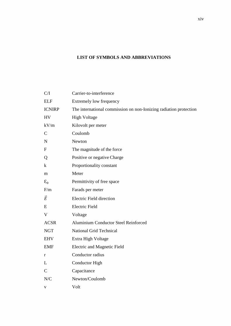
LIST OF SYMBOLS AND ABBREVIATIONS
C/I Carrier-to-interference
ELF Extremely low frequency
ICNIRP The international commission on non-Ionizing radiation protection
HV High Voltage
kV/m Kilovolt per meter
C Coulomb
N Newton
F The magnitude of the force
Q Positive or negative Charge
k Proportionality constant
m Meter
Permittivity of free space
F/m Farads per meter
Electric Field direction
E Electric Field
V Voltage
ACSR Aluminium Conductor Steel Reinforced
NGT National Grid Technical
EHV Extra High Voltage
EMF Electric and Magnetic Field
r Conductor radius
L Conductor High
C Capacitance
N/C Newton/Coulomb
v Volt
CHAPTER I
INTRODUCTION
1.1 Background
Electric power transmission is the bulk transfer of electrical energy from generating
power plants to electrical substations located near demand centres. Besides the power
transmission line is one of the most important components of electrical power
system. It is the main function to transfer the electric energy with minimal losses
from the power source to the load centres, usually separated by long distance.
An electric field surrounds electrically charged particles and time-varying.
The electric field depicts the force exerted on other electrically charged objects by
the electrically charged particle the field is surrounding. The concept of an electric
field was introduced by Michael Faraday. [1]. Electrical discharge that always occurs
from a space might be responsible for the electrostatic hazard such as the explosion
of a super tanker and gasoline tank. Meanwhile, So many phenomena can be
explained in terms of the electric field, but not nearly as well in terms of charges
simply exerting forces on each other through empty space, that electric field is
regarded as having a real physical existence, rather than being a mere
mathematically-defined quantity. For example when a collection of charges in one
region of space move, the effect on a test charge at a distant point is not felt
instantaneously, but instead is detected with a time delay that corresponds to the
changed pattern of electric field values moving through space at the speed of light.
2
That electric field strength submitted is the ratio of the force on a positive test charge
at rest to the magnitude of the test charge in the limit as the magnitude of the test
charge approaches zero. It has a special unit of volts per meter ( ) [2].
Furthermore, several critical parameters may affect the operability and
availability of power lines. Due to temperature and aging effects, the sag of the
conductor changes and may extend to a critical state which is the minimum distance
to objects in the environment that may not be guaranteed with adequate safety
margins. Another important aspect is icing of the power line as it constitutes
additional weight and may further increase the sag.
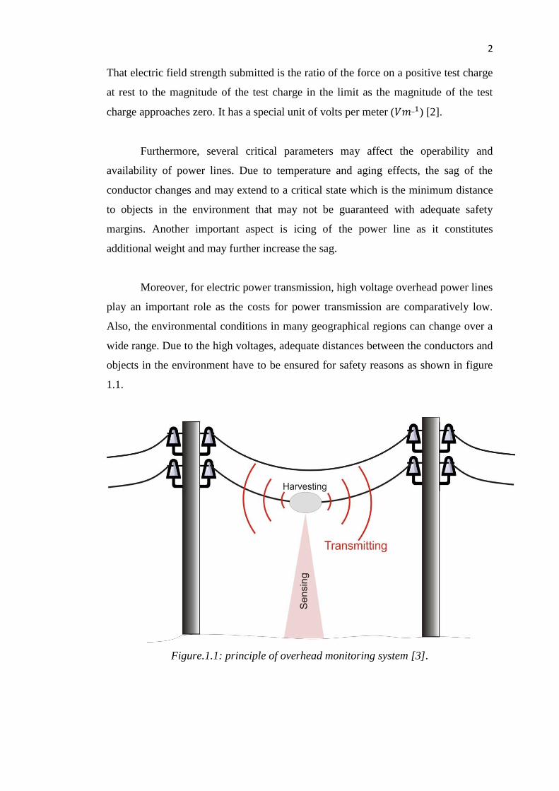
Moreover, for electric power transmission, high voltage overhead power lines
play an important role as the costs for power transmission are comparatively low.
Also, the environmental conditions in many geographical regions can change over a
wide range. Due to the high voltages, adequate distances between the conductors and
objects in the environment have to be ensured for safety reasons as shown in figure
1.1.
Figure.1.1: principle of overhead monitoring system [3].
3
In other word, sag of the conductors due to temperature variations or aging, icing of
conductors as a result of extreme weather conditions may increase safety margins
and limit the operability of the power lines.
Heavy loads due to icing or vibrations excited by winds increase the risk of
line breakage. With online condition monitoring of power lines, critical states or
states with increased wear for the conductor may be detected early and appropriate
counter measures can be applied[3,4].
1.2 Project Questions
This research will be conducted to answer the following questions:
i. What is the existing method of analyzing or measuring electric field strength?
ii. Have researches been done on the electric field strength in underneath
overhead power lines?
iii. What are the requirements needed to analysis the electric field strength
underneath overhead power lines?
iv. What is the significance of analyzing electric field strength underneath
overhead power lines?
1.3 Problem Statement
One of the applications of electric field strength its implementation in radio planning
process as an accurate estimation of propagating power loss. This provides a way for
determination of the electric field strength, carrier-to-interference (C/I) ratio and all
other parameters necessary for proper radio design [5].
4
Researchers have done that for measuring the electric-field intensity in the
near field, the characteristics of the top-loaded short dipole antenna is studied
theoretically and applied to an electric field measurement system [6].
However, there have been lesser researches on the analysis of electric field
strength propagating in the overhead power lines. Thus, this research intends to
analysis the electric field strength that is propagating underneath overhead power
lines.
To know the effects of electric field for human health, and let the people
know how much effect of electric field. 132 kV overhead line has selected to be the
case of study in this project because this type used in the area which near the
building.
1.4 Project Objectives
The primary objective of this study is to analysis the electric field strength
propagating underneath 132 kV overhead power line. In line with this primary
objective the secondary objectives are as following.
i. To define the possible method enabling calculating the electric field
underneath the 132 kV line.
ii. To calculate the electric field strength propagated by the 132 kV line at some
points above the ground level.
iii. To analysis the finding result with the guideline limits such public and
occupational exposure as defined in the international standard.
5
1.5 Project Scope
In order to achieve the objectives, the scopes have been highlighted such as:
i- To analyses the standard 132 kV overhead tower designs.
ii- To determine the correct method for analyzing or measuring electric field
strength.
iii- To validate of the results with researches have been done on electric field
strength underneath overhead power line.
iv- To analysis the outcomes result with the guideline limit set by
international standard appropriate simulation software.
CHAPTER II
LITERATURE REVIEW
2.1 Previous Study
R. Amiri, H Hadi, M. Marich from department of electrical engineering, faculty of genie
electric, university of sciences and technology of Oran, Mohamed Boudiaf, has
presented work for the influence of sag in the electric field calculation around high
voltage overhead transmission lines. Precise analytical modeling and quantization of
electric field produced by overhead power lines is important in several research areas.
Considerable research and public attention is concentrated on possible health effects of
extremely low frequency (ELF) electric field .In annual report conference on electric
insulation and dielectric phenomena in 2006 [7].
During the last 25 years, electric fields have been considered more and more as
environmental factors. The international commission on non-Ionizing radiation
protection (ICNIRP) published in 1998 the guidelines Analytical calculation of the
electric field produced by Single-circuit power lines has presented in IEEE transactions
on power delivery vol, on 3 July 2008 by A.E. Tzinevrakis [8].
Today electromagnetic environment has become the critical factor which
determines the construction of power transmission lines. Therefore, it is necessary to
analysis the distribution of electric field under the HV overhead lines especially in the
7
residential area. In June 2009, Zhujinglin and Mengyu from Shanghai electric power
design Institute Co Ltd they have studied the analysis of power frequency electric field
for the buildings under the high voltage overhead lines [9].
S.S. Razavipour, M. Jahangiri, H. Sadeghipoor in 2012 has studied electrical
field around the overhead transmission lines. In today’s world, an increasing level of
sensibility to health and ecological problems is seen. High-voltage overhead lines
generate electric and magnetic fields in their neighborhood. The electric field is caused
by the high potential of the conductors [10].
2.2 Electric Field
Electric field strength, E, is a function of voltage change around the line, expressed in
units of kilovolt per meter (kVm-1). These fields can be felt near transmission lines
through the coupling of voltages and current on motor vehicles or other metallic objects.
Increasing the voltage level will increase electric field strength [11].
An electric field is said to exist in a region of space if an electrical charge, at rest
in that space, experiences a force of electrical origin (i.e. electric fields cause free
charges to move). Electric field is a vector quantity that has both magnitude and
direction the direction corresponds to the direction that a positive charge would move in
the field. Sources of electric fields are unbalanced electrical charges (positive or
negative). Transmission lines, distribution lines, house wiring, and appliances generate
electric fields in their vicinity because of the unbalanced electrical charges associated
with voltage on the conductors.
The spatial uniformity of an electric field depends on the source of the field and
the distance from that source. On the ground under a transmission line the electric field
is nearly constant in magnitude and direction over distances of several feet (1 meter).
8
However, close to transmission or distribution line conductors, the field decreases
rapidly with distance from the conductors. Similarly near small sources such as
appliances, the field is not uniform and falls off even more rapidly with distance from
the device. If an energized conductor (source) is inside a grounded conducting
enclosure, then the electric field outside the enclosure is zero, and the source is said to
be shielded.
Electric fields interact with the charges in all matter, including living systems.
When a conducting object, such as a vehicle or person, is located in a time-varying
electric field near a transmission line, the external electric field exerts forces on the
charges in the object, and electric fields and currents are induced in the object. If the
object is grounded, then the total current induced in the body (the "short-circuit current")
flows to earth. The distribution of the currents within, say, the human body, depends on
the electrical conductivities of various parts of the body: for example, muscle and blood
have higher conductivity than bone and would therefore experience higher currents.
At the boundary surface between air and the conducting object, the field in the
air is perpendicular to the conductor surface and is much, much larger than the field in
the conductor itself. For example, the average surface field on a human standing in a 10
kV/m field is 27 kV/m; the internal fields in the body are much smaller: approximately
0.008 V/m in the torso and 0.45 V/m in the ankles [12].
2.2.1 Transmission line Electric Field
The electric field created by a high-voltage transmission line extends from the energized
conductors to other conducting objects such as the ground, towers, vegetation, buildings,
vehicles, and people. The calculated strength of the electric field at a height of 3.28 ft. (1
m) above an unvegetated, flat earth is frequently used to describe the electric field under
straight parallel transmission lines. The most important transmission-line parameters that
9
determine the electric field at a 1-m height are conductor height above ground and line
voltage [12].
Calculations of electric fields from transmission lines are performed with
computer programs based on well-known physical principles. The calculated values
under these conditions represent an ideal situation. When practical conditions approach
this ideal model, measurements and calculations agree. Often, however, conditions are
far from ideal because of variable terrain and vegetation. In these cases, fields are
calculated for ideal conditions, with the lowest conductor clearances to provide upper
bounds on the electric field under the transmission lines. With the use of more complex
models or empirical results, it is also possible to account accurately for variations in
conductor height, topography, and changes in line direction. Because the fields from
different sources add vector ally, it is possible to compute the fields from several
different lines if the electrical and geometrical properties of the lines are known.
However, in general, electric fields near transmission lines with vegetation below are
highly complex and cannot be calculated. Measured fields in such situations are highly
variable [13].
There are standard techniques for measuring transmission-line electric fields
(IEEE, 1987). Provided that the conditions at a measurement site closely approximate
those of the ideal situation assumed for calculations, measurements of electric fields
agree well with the calculated values. If the ideal conditions are not approximated, the
measured field can differ substantially from calculated values. Usually the actual electric
field at ground level is reduced from the calculated values by various common objects
that act as shields.
Maximum or peak field values occur over a small area at mid span, where
conductors are closest to the ground (minimum clearance). As the location of an electric-
field profile approaches a tower, the conductor clearance increases, and the peak field
decreases. A grounded tower will reduce the electric field considerably by shielding.
10
For traditional transmission lines, such as the proposed line, where the right-of-way
extends laterally well beyond the conductors, electric fields at the edge of the right-of-
way are not as sensitive as the peak field to conductor height. Computed values at the
edge of the right-of-way for any line height are fairly representative of what can be
expected all along the transmission-line corridor. However, the presence of vegetation
on and at the edge of the right-of-way will reduce actual electric-field levels below
calculated values [13].
2.2.2 Theory of the Electric Field on Transmission Lines
They are also called force lines.
The field lines are originated from the positive charge.
The field lines end up at the negative charge.
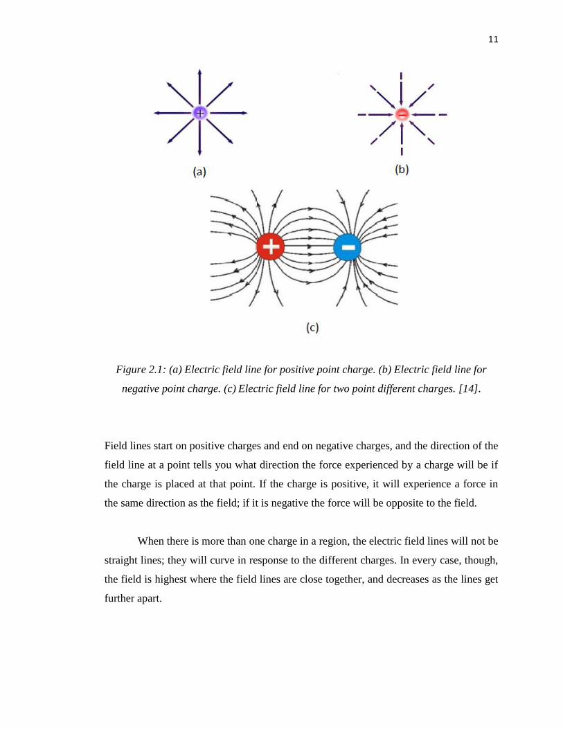
A positive charge exerts out and a negative charge exerts in equally to all directions,
it is symmetric. Field lines are drawn to show the direction and strength of field. The
closer the lines are, the stronger the force acts on an object. If the lines are further each
other, the strength of force acting on an object is weaker [14].Figure 2.1 shown the
positive charge, negative charge and two point different charges
11
Figure 2.1: (a) Electric field line for positive point charge. (b) Electric field line for
negative point charge. (c) Electric field line for two point different charges. [14].
Field lines start on positive charges and end on negative charges, and the direction of the
field line at a point tells you what direction the force experienced by a charge will be if
the charge is placed at that point. If the charge is positive, it will experience a force in
the same direction as the field; if it is negative the force will be opposite to the field.
When there is more than one charge in a region, the electric field lines will not be
straight lines; they will curve in response to the different charges. In every case, though,
the field is highest where the field lines are close together, and decreases as the lines get
further apart.
12
2.3 Electrostatic Field
Electricity is an essential part of our lives. It powers our appliances, office equipment
and countless other devices that we use to make life safer, easier and more interesting.
Use of electric power is something many of us take for granted. Some have wondered
whether long-term public exposure to electric and magnetic fields produced through the
generation, transmission and use of electric power might adversely affect our health
[14].
An electrostatic field is an electric field produced by static electric charges. The
charges are static in the sense of charge amount it is constant in time and their positions
in space charges are not moving relatively to each other. Due to its simple nature, the
electrostatic field or its visible manifestation electrostatic force - has been observed long
time ago. Even ancient Greeks knew something about a strange property of amber that
attracts under certain conditions small and light pieces of matter in its vicinity. Much
later this phenomenon has been understood and explained as an effect of the electrostatic
field. From this historical viewpoint, it would be logical to start the presentation of
electromagnetic field theory with electrostatic field. Another reason, as it will be later
clear, is its simplicity but also applicability. Namely, electrostatic field plays an
important role in modern design of electromagnetic devices whenever a strong electric
field appears. For example, an electric field is of paramount importance for the design of
X-ray devices, lightning protection equipment and high-voltage components of electric
power transmission systems, and hence an analysis of electrostatic field is needed. This
is not only important for high-power applications. In the area of solid-state electronics,
dealing with electrostatics is inevitable. It is sufficient to mention only the most
prominent examples, such as resistors, capacitors or bipolar and field-effect transistors.
Concerning computer and other electronic equipment, the situation seems to be similar:
cathode ray tubes, liquid crystal display, touch pads etc. [12, 13].
13
2.3.1 Electric Charge
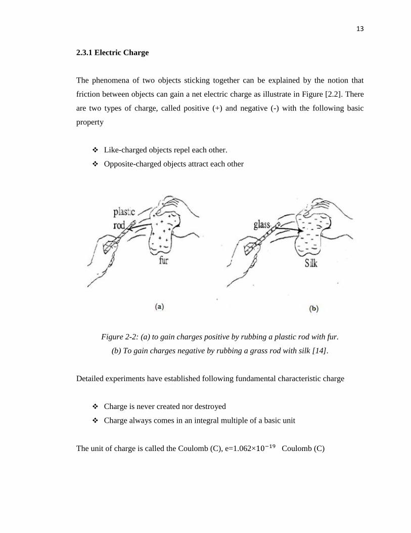
The phenomena of two objects sticking together can be explained by the notion that
friction between objects can gain a net electric charge as illustrate in Figure [2.2]. There
are two types of charge, called positive (+) and negative (-) with the following basic
property
Like-charged objects repel each other.
Opposite-charged objects attract each other
Figure 2-2: (a) to gain charges positive by rubbing a plastic rod with fur.
(b) To gain charges negative by rubbing a grass rod with silk [14].
Detailed experiments have established following fundamental characteristic charge
Charge is never created nor destroyed
Charge always comes in an integral multiple of a basic unit
The unit of charge is called the Coulomb (C), e=1.062× Coulomb (C)
14
2.3.2 Coulomb’s Law
The electric interaction between two charged particles is described in terms of the forces
they exert on each other. Charles Augustin de Coulomb (1786-1803) using an invented
tension balance to determine quantitatively the force electric exerted between two objects
where each having a static charge of electricity. He states that the force between two
charged particles separated in a vacuum or free space by a distance is directly proportional
to the product of charges and inversely proportional to the square of the distance between
them. The magnitude of the force of attraction or repulsion is given by Coulomb's Law
as standard in equation (2.1).
0 (Newton) [14] (2.1)
Where Q1 and Q2 are the positive or negative quantities of charger, R is the
separation and k is proportionality constant. If SI unit is used Q is measured in
coulombs(C), R is meters (m) and force should be Newton (N). This will be achieved if
the constant of proportionality k as is written as
[14] (2.2)
N
The constant is called the permittivity of free space and has magnitude measured in
farads per meter F/m;
[14] (2.3)
Figure 2.3 shown the direction of the force F
15
F2
R12
r2S(X’,Y’,Z’)
Origin
P(x,y,z)
Q1
Q2
r1
a12^
0
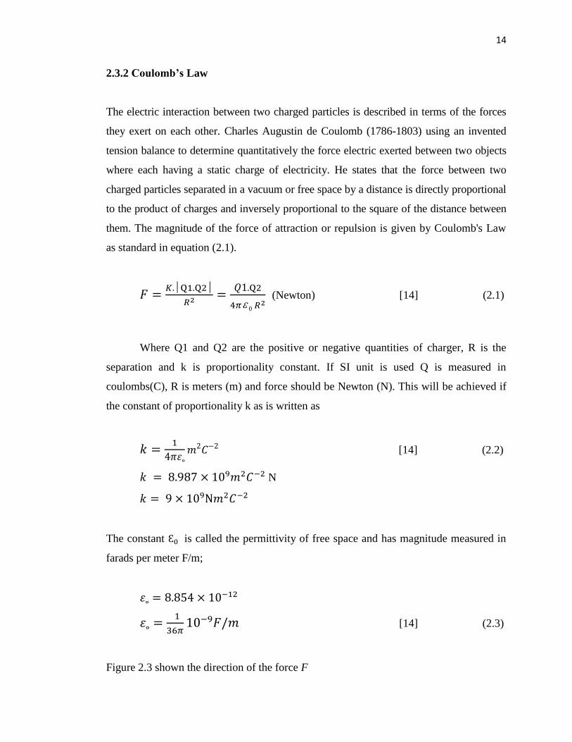
Figure 2.3: If Q1 and Q2 have like signs, the vector force F.2 on Q2 is in the same
direction as the vector [14].
Consider Q1 and Q2 are two charges particles located S (x’, y’, z’) and P(x, y, z) with
vector and respectively. The vector
= respectively the directed line segment Q1 to Q2 as shown in figure 2.2 The vector
is the force on Q2 and is shown for the case where from Q1 to Q2 have the same
sign. The vector from Coulomb’s law is [14].
0 [14] (2.4)
Where:
12=
=
=
16
2.3.3 Potential Difference and Potential
Potential difference is defined as work done in moving a unit positive charge from one
point to other in an electric filed. It is a location dependent quantity which expresses the
amount of potential energy DW per unit charge
[21] (2.5)
The potential difference between points A and B in a circuit is commonly
referred as voltage calculated as integration the path taken from B to A.
∫
(
) [21] (2.6)
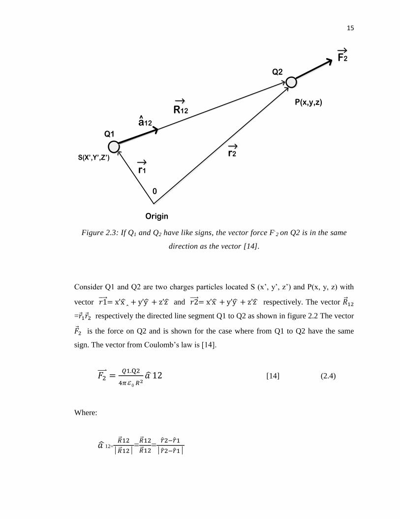
is positive if work is done in carrying the positive charge from B to A. The
SI unit of potential difference is the volt (V) or joules per coulomb. Consider the
potential difference between point A and B in the field of a point charge Q placed at the
origin as shown in the figure 2.4.[21].
Figure 2.4 A path between points B and A in the field of point charge at origin [21].
17
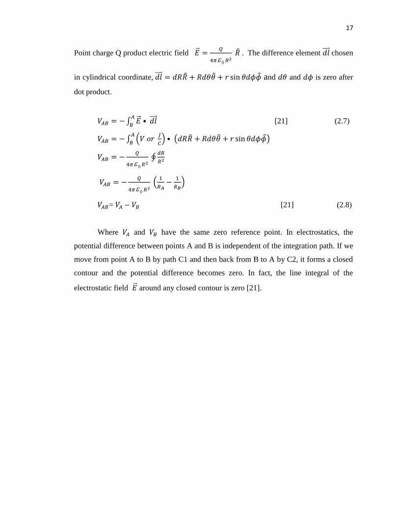
Point charge Q product electric field
0 . The difference element chosen
in cylindrical coordinate, and and is zero after
dot product.
∫
[21] (2.7)
∫ (
)
( )
0 ∮
0 (
)
= [21] (2.8)
Where and have the same zero reference point. In electrostatics, the
potential difference between points A and B is independent of the integration path. If we
move from point A to B by path C1 and then back from B to A by C2, it forms a closed
contour and the potential difference becomes zero. In fact, the line integral of the
electrostatic field around any closed contour is zero [21].
18
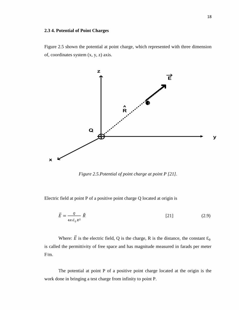
2.3 4. Potential of Point Charges
Figure 2.5 shown the potential at point charge, which represented with three dimension
of, coordinates system (x, y, z) axis.
E
z
Q
y
x
R^
Figure 2.5.Potential of point charge at point P [21].
Electric field at point P of a positive point charge Q located at origin is
0 [21] (2.9)
Where: is the electric field, Q is the charge, R is the distance, the constant
is called the permittivity of free space and has magnitude measured in farads per meter
F/m.
The potential at point P of a positive point charge located at the origin is the
work done in bringing a test charge from infinity to point P.
19
∫
[21] (2.10)
∫ (
0 )
( )
∫
0
0 (V) [21] (2.11)
If the charge Q is at a location other than the origin, specified by a source
position vector , then V at observation position vector becomes
0 | | [21] (2.12)
where | | is the distance between the observation point and the location of
the charge Q.
For N discrete point charges , ,..., , we use the principle of superposition and
add the potentials due to the individual charges.
0∑
| |
(V) [21] (2.13)
For continuous charge distribution, we use the principle of integral. The general
expression for potential of continuous distribution is
∫
0
0∫
[21] (2.14)
20
The concept of continuous charge distribution can be applied to determine potential due
to line, surface and volume charge distribution [21].
The expression assistant
0∫
(Line charge distribution) [21] (2.15)
0∫
(Surface charge distribution) [21] (2.16)
0∫
(Volume charge distribution) [21] (2.17)
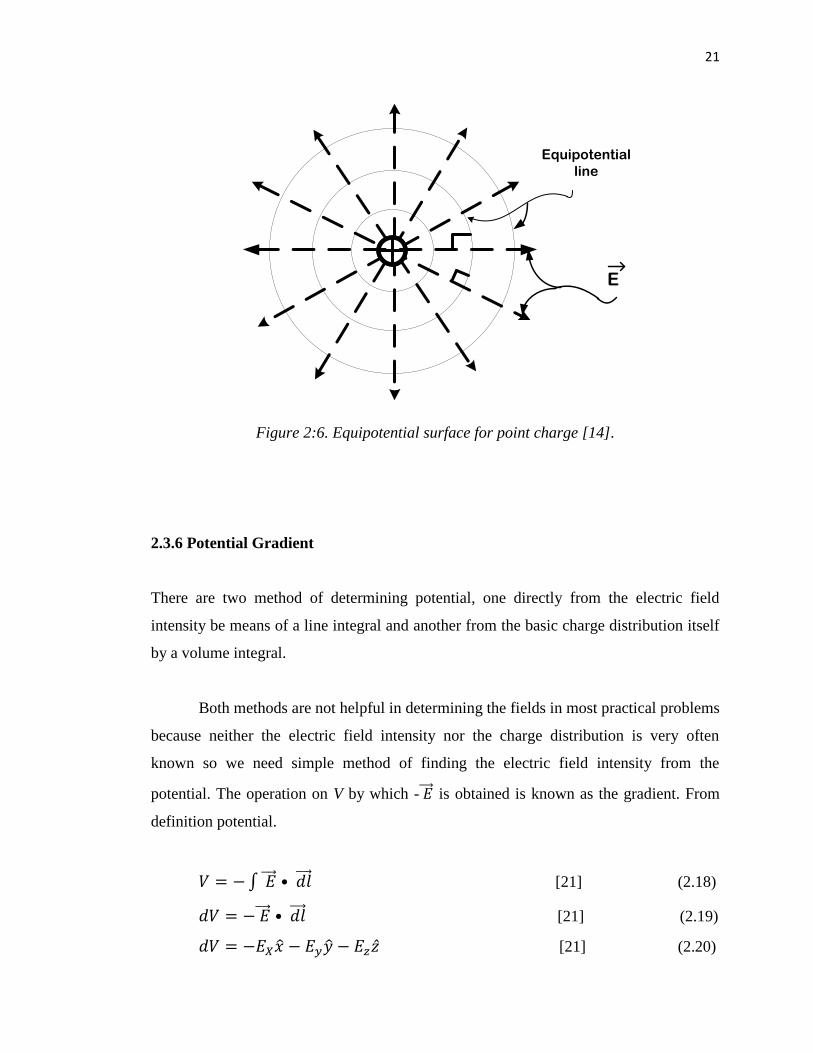
2.3.5 Equipotential Surface
Filed lines help us to visualize electric fields. In a similar way the potential at various in
an electric field can be described by equipotential surface where each corresponds to a
different fixed value of the potential.
An equipotential surface is surface each the every point in the surface has the
same potential. The equipotential surface through any point must be perpendicular to the
direction of the field at the point. Field lines and equipotential surface are always
mutually perpendicular. If a charge moves along an equipotential line, no work done; if
a charge moves between equipotential lines, work is done [14].figure 2.6 shown
Equipotential surface for point charge.
21
E
Equipotential
line
Figure 2:6. Equipotential surface for point charge [14].
2.3.6 Potential Gradient
There are two method of determining potential, one directly from the electric field
intensity be means of a line integral and another from the basic charge distribution itself
by a volume integral.
Both methods are not helpful in determining the fields in most practical problems
because neither the electric field intensity nor the charge distribution is very often
known so we need simple method of finding the electric field intensity from the
potential. The operation on V by which - is obtained is known as the gradient. From
definition potential.
∫ [21] (2.18)
[21] (2.19)
[21] (2.20)
22
Equation dV equivalent with
[21] (2.21)
Compare equations (2, 20) and (2, 21)
or
[21] (2.22)
Where is opposite with gradient V. Negative sigh show that direction of is opposite
with direction of increasing V, which is direct from maximum to minimum potential.
That gradient may be expressed in term of partial derivatives in Cartesian, Cylindrical,
or spherical coordinate systems [21].
(Cartesian) [21] (2.23)
(Cylindrical) [21] (2.24)
(Spherical) [21] (2.25)
23
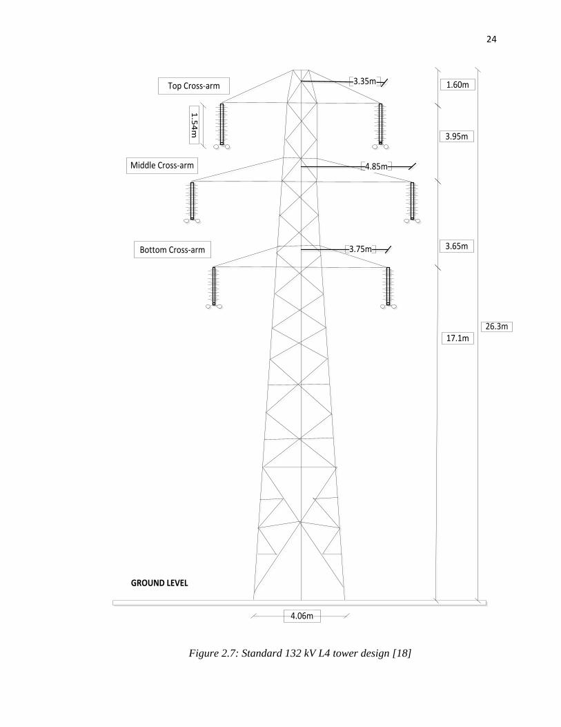
2.4 Configuration 132 kV Tower (case of study)
The work is based on the analysis of a 132 kV tower as used on the National Grid
system. This is one of the most common tower types and was therefore selected for
analysis, this type of the tower is can be found in the area which near from the building
in cites, dimensions and scales for 132 kV overhead line as shown in Figure 2.7.
The 132 kV L4 overhead lines composed of the tower body which made of steel
the tower high is 26 meters above the ground. The 132 kV L4 has six conductors the
Aluminium Conductor Steel Reinforced (ACSR) used in this type of tower. One of the
most important and yet one of the most vulnerable links in transmission and distribution
is insulators. Porcelain and toughened glass are the materials principally used for
supporting conductors on overhead lines, and although these materials are relatively
brittle and inelastic, they have proven service experience and are still widely used. The
poles carry 3-phase conductors (cables) in a single circuit network with an under slung
earth wire, which incorporates a fibre optic cable for protection signalling and
communication purposes, The minimum ground clearance distance for a 132kv overhead
line is 6.7m (including the lower earth wire) and the overhead line is designed to ensure
this distance is maintained at all times and in all conditions.132 kV has three cross-arms
are steel construction made [15].
24
3.75m
4.85m
3.35m
GROUND LEVEL
4.06m
1.60m
3.95m
3.65m
17.1m26.3m
Top Cross-arm
Middle Cross-arm
Bottom Cross-arm
1.5
4m
Figure 2.7: Standard 132 kV L4 tower design [18]
REFERENCES
[1] Research of Electric-field Strength Measurement Based on a Top-loaded Antenna in the Near
Field. Bin, Y. Z. Xiang, C. & Jiahong, C. (2008). Asia-Pacific Symposium on Electromagnetic
Compatibility & 19th International Zurich Symposium on Electromagnetic Compatibility, pp.
602 – 605.
[2] Electric fields from: http//:www.equipotentiallines.com, retrieved on 10th December,
2011. (Access in 13 Jan 2013).
[3] Energy Harvesting For Onli Condition Monitoring Of Voltage Overhead Power Lines.
Hubert, Z.,Thomas, B. & Georg, B. (2008). MTC-IEEE International Instrumentation and
Measurement Technology Conference, pp. 1-6.
[4] Arrangement Of Overhead Power Line Conductors Related To The Electromagnetic Field
Limits. Klemen, D. Goradzd , S. & Franc, J. (2010). Modern Electric Power Systems, pp
[5] Zeljkovic, N., Gusavac, V., Neskovic, A. & Paunovic, D. (2005) Dependence of Electric
Field Strength Prediction Model Accuracy on Database Resolution. EUROCON, pp. 1783-1786.
[6] Wu, Y., Castle, G. S. P., Inculet, I. I., Petigny, S. & Swei, G. (2003) Induction Charge on
Freely Levitating Particles. Journal of Powder Technol vol. 135–136, pp. 59-64.
[7] Department of electrical engineering department of electrical engineering, faculty of
genie electric, university of sciences and technology of Oran, Mohamed Boudiaf, R. Amiri,
H Hadi, M. Marich. (2006), influence of sag in the electric field calculation around high
voltage overhead transmission lines.
58
[8] Analytical calculation of the electric field produced by Single-circuit power line. A E
Tzinevrakis IEEE transactions on power delivery vol, on 3 July 2008.
[9] Analysis of power frequency electric field for the buildings under the high voltage overhead
lines Zhujinglin and Mengyu .20th International Conference on Electricity Distribution Prague,
8-11 June 2009 Paper 0306.
[10] Electrical Field around the overhead Transmission Lines. S.S. Razavipour, M. Jahangiri, H.
Sadeghipoor. World Academy of Science, Engineering and Technology 62 2012 .
[11] Overhead Line Design Methods Concerning Electromagnetic Fields, Lightning, Corona
Loss and Radio/Audible Noise .Dr. MD NOR RAMDON BIN BAHAROM.
[12] Electromagnetic Field theory Second Tobia Carozzi, Anders Eriksson, Bengt Lundborg,,
Bo Thidé and Mattias Waldenvik Copyright 1997–2009.
[13] Big Eddy – Knight 500-kv Transmission Project. T. Dan Bracken, Inc Bonneville Power
Administration March 2010.
[14] Concepts of electromagnetics (first edition) chua king lee and mohd zarar mohd jenu
Faculty of Electric &Electronic Engineering Universiti Tun Hussein Onn Malaysia 2007.
[15] Line Mannal M1 for 132, 275, and 400kV overhead lines.24th April 1989.natinal technical
training centre. Handbook.
[16] Mohtar, S. N. Jamal, M. N. & Sulaiman. M. Analysis of All Aluminum Conductors (AAC)
and All Aluminum Alloy Conductors (AAAC), IEEE.
[17] Condudtor bundles for overhead lines, PS (T) 046 – issue 1-October 2004 National Grid
Transco.
[18] National Grid internal and contract specific Technical Specification.Insulator ets for
overhead lines TS 3.4.17- Issue 2- September 2006.
59
[19] Insulation co-ordination. Computational guide to insulation co-ordination and modeling
of electrical IEC60071-1 part 1.
[20] EMF Exposure Standards Applicable in Europe and Elsewhere. Environment & Society
Working Group. May 2003 Ref 2003 - 450 – 0007.
[21] Extra high voltage AC transmission engineering (Third edition) Rokosh Das Begamudre
Copyright9©2006, 1990, 1986, New Age International (P) Ltd, Publishers.