Fourth International Symposium on Marine Propulsors smp’15, Austin, Texas, USA, June 2015

Analysis of Ducted Propellers by Combining

Potential Flow and RANS Methods

Johan Bosschers1, Chris Willemsen

2, Adam Peddle

3, Douwe Rijpkema

4

1,4 Maritime Research Institute Netherlands, MARIN, Wageningen, The Netherlands 2 University of Twente, Enschede, The Netherlands, presently at MARIN

3 MARIN, presently at University of Exeter, Exeter, Devon UK.

ABSTRACT

An iterative procedure to analyze ducted propellers in open

water conditions using a combination of a RANS solver and

a boundary element method (BEM) has been developed and

tested. The RANS solver analyses the viscous flow over the

duct modeling the propeller through the use of body forces.

These body forces are obtained from the BEM in which

both duct and propeller are analyzed. In the BEM solution

the loading on the duct is prescribed and obtained from the

RANS solution. The results of this procedure are compared

with results obtained from a full RANS and a full BEM

computation and with experimental data.

Keywords

Ducted Propellers, BEM, RANS.

NOMENCLATURE

n Shaft rotation rate [rev/s]

p Pressure [Pa]

p Free-stream pressure [Pa]

D Propeller diameter [m]

Density of fluid [kg/m3]

V Free-stream velocity [m/s]

pnC Pressure coefficient,

2 212pnC p p n D

J Advance ratio, J V nD

RF Radial force coefficient,

2 4RadialForce[N]RF n D

TK Thrust coefficient,

2 4Thrust[ ]TK N n D

QK Torque coefficient,

2 5Torque[Nm]QK n D

Efficiency,

, , ,2T prop T duct Q propJ K K K

pre

1 INTRODUCTION

The analysis and design of propellers using boundary

element methods (BEM) that solve the potential flow

equations is common practice in the marine industry.

However, the analysis of ducted propellers is still

challenging when only boundary element methods are used

as there are a number of features in this flow that cannot be

captured by potential flow. Some of these features are given

in Figure 1. The boundary layer on the inner surface of the

duct influences the loading on the propeller, the flow

through the gap and the convection of the vortices generated

at the tip of the propeller. The gap leads to the generation of

a tip leakage vortex that influences the loading on the

propeller blade. At the blunt trailing edge of the duct flow

separation will occur that can not be captured by potential

flow. The location of the separation point at the blunt

trailing edge is very important as it influences the loading

on the duct. The last item shown in Figure 1 is the presence

of flow separation on the outer surface near the leading

edge of the duct that may occur for high advance ratios.

Baltazar et al. (2012) have shown that a BEM is able to give

a good prediction of the open water characteristics for a

duct with a sharp trailing edge provided the velocity defect

due to the duct boundary layer is used in the iterative wake

alignment procedure. The influence of the velocity through

the gap was shown to be small. At higher advance ratios the

prediction of especially the duct thrust was not so good due

to the occurrence of flow separation on the duct.

The viscous flow features are captured by solving the

Reynolds-Averaged Navier-Stokes (RANS) equations but

the grid generation is more complex and much more

computational resources are required. For that reason there

is still a demand for BEM computations by for instance

propeller designers. A comparison between BEM

computations and RANS computations for a ducted

propeller with a neutral duct is presented by Baltazar et al

(2013).

Figure 1: Typical flow features for a ducted

propeller influenced by viscosity; (1) boundary layer inner

duct surface; (2) gap flow; (3) flow separation at the blunt

trailing edge; (4) flow separation on the outer surface of the

duct for low propeller loading. The colour coding represents

the circumferential component of vorticity computed by a

full RANS solution at high advance ratio.

In the present paper an iterative procedure for the analysis

of ducted propellers in open water conditions using a

combination of a RANS solver and BEM is used to capture

some of the viscous flow features given in Figure 1, being

the flow over the blunt trailing edge, the flow separation

near the leading edge for high advance ratios and the

boundary layer on the inner duct surface.

A coupling between RANS and BEM has already been

developed for the analysis of the propulsive performance of

ships. The viscous flow over the ship hull has been analyzed

with a RANS solver taking the propeller action into account

by using body forces obtained from the BEM (Starke &

Bosschers, 2012 and Rijpkema et al. 2013). We will show

here a somewhat similar approach by analysing the viscous

flow for the duct using RANS in which body forces are

used to represent the propeller action. These body forces are

obtained from the solution computed by BEM in which the

duct is taken into account but the blunt trailing edge has

been made sharp. A procedure has been developed through

which the loading on the duct can be adjusted to a user

prescribed value that can be obtained from for instance the

RANS solution. This leads to an iterative method for the

viscous flow analysis of ducted propellers. The results of

this coupling procedure is compared with experimental data

for a Ka4-70 propeller with pitch P/D= 1.0 operating in a

19A duct. The geometry of this configuration is given by

Kuiper (1992).

The used numerical methods are described first in the next

section followed by a more detailed description of the

coupling procedure. Open water results of the full BEM (i.e.

without coupling to RANS) are first compared to

experiments, followed by the results of the coupled

approach. The loading and pressure distribution are then

compared in more detail with full RANS results. The paper

finishes with the conclusions and recommendations for

further work.

2 NUMERICAL METHODS AND GRIDS

2.1 PROCAL

The boundary element method that is used to solve the

incompressible potential flow is the PROCAL code.

PROCAL has been developed by MARIN within the

Cooperative Research Ships (CRS1) for the unsteady

analysis of cavitating propellers operating in a prescribed

ship wake and is currently in development for the analysis

of ducted propellers. It has been validated for open water

characteristics, shaft forces and moments, sheet cavitation

extents and propeller induced hull-pressure fluctuations.

The code is a low order BEM that solves for the velocity

disturbance potential using the Morino formulation. Initial

validation studies and details on the mathematical and

numerical model can be found in Vaz & Bosschers (2006)

and Bosschers et. al (2008). The geometry of the blade

wake can be determined by an iterative procedure to align

the propeller wake with the flow or by using a prescribed

wake pitch and contraction using empirical formulations to

reduce CPU time.

For the analysis of ducted propellers a similar method as

proposed by Baltazar et al. (2012) has been implemented.

An iterative wake alignment method is used for the wake of

the propeller and duct in which the radial position of the

trailing vortices is prescribed while the pitch is obtained

from the computed induced velocities. The induced

velocities near the duct surface are reduced depending on a

user specified boundary layer thickness. The gap between

propeller blade and duct is modeled as a surface on which

the transpiration velocity can be prescribed according to a

user specified value or using the gap model of Kerwin et al.

(1987). Unless otherwise specified, the transpiration

velocity in the gap is neglected by default and the gap is

modeled as a rigid surface. The duct trailing edge geometry

is modified such that a sharp trailing edge is present and the

location from which the vortices trail from the duct is

clearly defined. An iterative pressure Kutta condition is

applied in which the duct and propeller wake strength is

modified until the pressure difference on the two surfaces at

the trailing edge of blade and duct is smaller than a user

specified value. Results of PROCAL for ducted propellers

are also presented by Moulijn (2015).

The grid on the propeller blade, hub, gap and duct is

generated by the computer code with graphical user

1 www.crships.org

interface PROVISE, developed by DRDC Atlantic within

the CRS. An example of the grid is shown in Figure 2.

2.2 REFRESCO

ReFRESCO is a viscous-flow CFD code that solves

multiphase (unsteady) incompressible flows using the

RANS equations, complemented with turbulence models,

cavitation models and volume-fraction transport equations

for different phases, Vaz et al.(2009). The equations are

discretised using a finite-volume approach with cell-

centered collocated variables, in strong-conservation form,

and a pressure-correction equation based on the SIMPLE

algorithm is used to ensure mass conservation. Time

integration is performed implicitly with first or second-

order backward schemes. At each implicit time step, the

non-linear system for velocity and pressure is linearised

with Picard’s method and either a segregated or coupled

approach is used. In the latter, the coupled linear system is

solved with a matrix-free Krylov subspace method using a

SIMPLE-type preconditioner, Klaij and Vuik (2013). A

segregated approach is always adopted for the solution of

all other transport equations. The implementation is face-

based, which permits grids with elements consisting of an

arbitrary number of faces (hexahedrals, tetrahedrals, prisms,

pyramids, etc.), and if needed h-refinement (hanging

nodes). State-of-the-art CFD features such as moving,

sliding and deforming grids, as well automatic grid

refinement are also available. For turbulence modeling,

RANS/URANS, SAS and DES approaches can be used

(PANS and LES are also being studied). The code is

parallelized using MPI and subdomain decomposition, and

runs on Linux workstations and HPC clusters. Application

of ReFRESCO for different propeller types is treated by

Rijpkema and Vaz (2011).

In the RANS simulations a k-ω SST turbulence model was

used. For the discretization of the convective flux of the

momentum and turbulence equations a QUICK and upwind

scheme were used respectively. For the boundary conditions

a uniform flow at the inlet and constant pressure at the

external boundary was applied. At the outlet, an outflow

boundary condition is prescribed with zero normal gradient

for the flow variables. For the full RANS simulations, a no-

slip boundary condition is set at the propeller blades, duct

and shaft. A rotational velocity is prescribed to the blades

and shaft, while the duct does not rotate. For open water

(steady) computations the equations are solved in the body-

fixed reference frame.

Figure 2: Example of a typical panel distribution on the

ducted propeller (Ka4-70 propeller with duct 19A).

Figure 3: Example of the grid for the full RANS

computations for propeller Ka4-70 and duct 19A.

Figure 4: Example of the RANS grid for the duct 19A

using body forces to represent the propeller action.

x

r

-1-0.500.511.5

0.2

0.4

0.6

0.8

1

1.2

1.4

1.6

1.8

2

2.2

An example of the grid layout for the full RANS

computations is presented in Figure 3 while the grid for the

RANS computations using body forces is shown in Figure

4. The y+-values for all grids are smaller than one with all

computations made for model scale conditions. The grid

sizes used are presented later.

3 RANS-BEM COUPLING PROCEDURE

3.1 Description

In the coupled approach the flow on propeller blade and

duct is analyzed with the BEM PROCAL. However, due to

the user generated sharp trailing geometry of the duct, an

error in the duct loading is likely to occur which may also

lead to an error in propeller blade loading. For that reason

the flow on the duct with unmodified trailing edge geometry

is analyzed with the RANS solver ReFRESCO. The

influence of the propeller blades is taken into account

through the use of body forces. The force distribution on the

blade camber surface in PROCAL is transferred from the

BEM grid to the RANS grid. In the present approach the 3-

D flow is analyzed but for open water conditions an

axisymmetric RANS solver can be used to reduce CPU

time.

The loading on the duct is likely to be different in viscous

flow simulations than in the potential flow computations.

As the loading on the duct influences the loading on the

propeller blade, the loading on the duct in the BEM needs to

be adjusted such that it is identical to the value obtained in

the RANS solver. This can be accomplished by applying

surface transpiration velocities on the duct which can be

interpreted as adding a boundary layer displacement

thickness to the duct which effectively changes the

thickness and camber of the duct. To simplify the

procedure, the variation of the boundary layer displacement

thickness with distance to the leading edge is prescribed and

is applied on the inner surface of the duct only. The value at

the duct trailing edge is then left as the only unknown. Its

value can either be prescribed by the user or it can be

obtained through an iterative procedure in which its value is

adjusted until an user specified duct force is obtained.

The resulting iterative procedure using a sequence of BEM

and RANS computations is sketched in Figure 5. In the

BEM computation the transpiration velocity on the duct is

modified until the duct force matches the value obtained

from the RANS computation. The resulting propeller force

distribution is then used to update the RANS computation.

The computations are repeated for a number of iterations

which are prescribed in advance at present. The

computational procedure starts with a BEM computation

without transpiration velocity.

Figure 5: The RANS-BEM coupling procedure for the

analysis of a ducted propeller in open water.

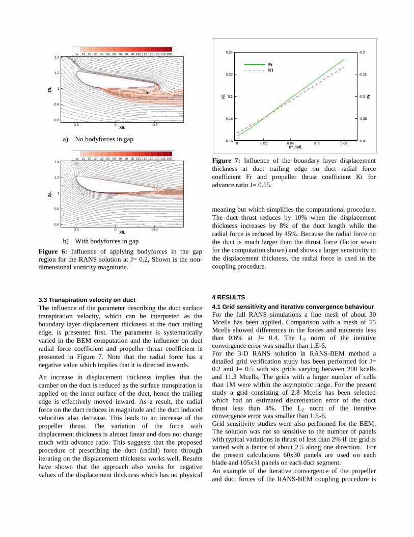
3.2 Applying body forces in RANS

Even though the application of body forces in the RANS

computations is rather straight forward, first results showed

a large region with flow separation on the inner surface of

the duct starting at the propeller tip for low advance ratio,

see Figure 6a. The flow separation only occurred for high

propeller loading at low advance ratio and disappeared for

lower propeller loadings. The separation was generated by

the high tip loading of the propeller which generated an

upstream directed velocity in the gap where no body force

was present. In reality a tip leakage vortex is generated in

this region but due to the axisymmetric flow in the RANS

simulations for the RANS-BEM coupling, no tip leakage

vortex can be generated and hence this flow separation is

considered a deficiency of the imposed axisymmetric flow

conditions. The separation could easily be avoided by

applying a body force in the gap region which can be

obtained from the BEM computation because the gap is also

discretized with dipole and monopole panels. The resulting

flow is shown in Figure 6b.

The separation bubble leads to a significant change in duct

loading with the duct thrust changing from , 0.117T ductK

for the situation without body forces in the gap to

, 0.173T ductK for the situation with body forces in the gap.

In the experiments a value of , 0.170T ductK was measured.

For advance ratios J= 0.5 and J= 0.8 the RANS results did

not show any influence of applying body forces in the gap

region because for these advance ratios flow separation did

not occur when no body forces were applied in the gap.

Therefore, all computations have been performed with body

forces in the gap region.

a) No bodyforces in gap

b) With bodyforces in gap

Figure 6: Influence of applying bodyforces in the gap

region for the RANS solution at J= 0.2, Shown is the non-

dimensional vorticity magnitude.

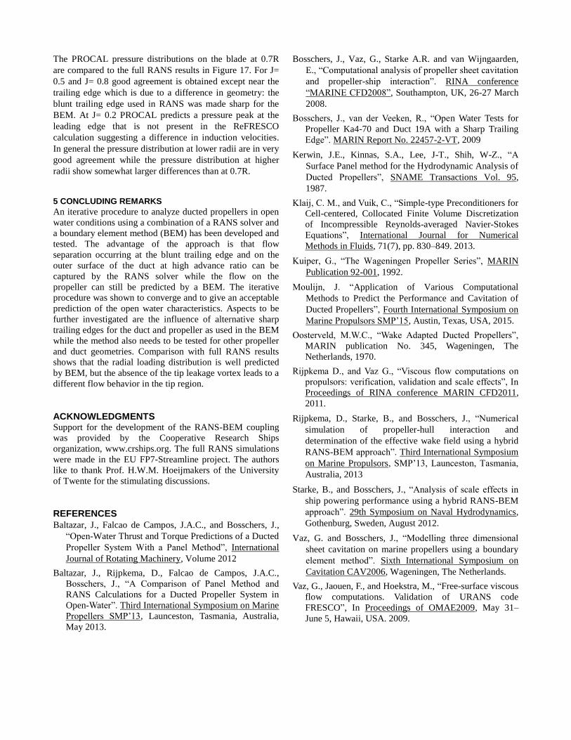
3.3 Transpiration velocity on duct

The influence of the parameter describing the duct surface

transpiration velocity, which can be interpreted as the

boundary layer displacement thickness at the duct trailing

edge, is presented first. The parameter is systematically

varied in the BEM computation and the influence on duct

radial force coefficient and propeller thrust coefficient is

presented in Figure 7. Note that the radial force has a

negative value which implies that it is directed inwards.

An increase in displacement thickness implies that the

camber on the duct is reduced as the surface transpiration is

applied on the inner surface of the duct, hence the trailing

edge is effectively moved inward. As a result, the radial

force on the duct reduces in magnitude and the duct induced

velocities also decrease. This leads to an increase of the

propeller thrust. The variation of the force with

displacement thickness is almost linear and does not change

much with advance ratio. This suggests that the proposed

procedure of prescribing the duct (radial) force through

iterating on the displacement thickness works well. Results

have shown that the approach also works for negative

values of the displacement thickness which has no physical

meaning but which simplifies the computational procedure.

The duct thrust reduces by 10% when the displacement

thickness increases by 8% of the duct length while the

radial force is reduced by 45%. Because the radial force on

the duct is much larger than the thrust force (factor seven

for the computation shown) and shows a larger sensitivity to

the displacement thickness, the radial force is used in the

coupling procedure.

4 RESULTS

4.1 Grid sensitivity and iterative convergence behaviour

For the full RANS simulations a fine mesh of about 30

Mcells has been applied. Comparison with a mesh of 55

Mcells showed differences in the forces and moments less

than 0.6% at J= 0.4. The L2 norm of the iterative

convergence error was smaller than 1.E-6.

For the 3-D RANS solution in RANS-BEM method a

detailed grid verification study has been performed for J=

0.2 and J= 0.5 with six grids varying between 200 kcells

and 11.3 Mcells. The grids with a larger number of cells

than 1M were within the asymptotic range. For the present

study a grid consisting of 2.8 Mcells has been selected

which had an estimated discretisation error of the duct

thrust less than 4%. The L2 norm of the iterative

convergence error was smaller than 1.E-6.

Grid sensitivity studies were also performed for the BEM.

The solution was not so sensitive to the number of panels

with typical variations in thrust of less than 2% if the grid is

varied with a factor of about 2.5 along one direction. For

the present calculations 60x30 panels are used on each

blade and 105x31 panels on each duct segment.

An example of the iterative convergence of the propeller

and duct forces of the RANS-BEM coupling procedure is

X/L

Z/L

-0.500.5

0.6

0.8

1

1.2

1.4w: 10 20 30 40 50 60 70 80 90 100 110 120 130 140 150

X/L

Z/L

-0.500.5

0.6

0.8

1

1.2

1.4w: 10 20 30 40 50 60 70 80 90 100 110 120 130 140 150

Figure 7: Influence of the boundary layer displacement

thickness at duct trailing edge on duct radial force

coefficient Fr and propeller thrust coefficient Kt for

advance ratio J= 0.55.

d*_te/L

Kt

Fr

0 0.02 0.04 0.06 0.080.16

0.18

0.2

0.22

0.24

-0.4

-0.35

-0.3

-0.25

-0.2

Fr

Kt

shown in Figure 8. Our initial procedure is to prescribe the

number of iterations in RANS, 500 for the present test-case,

after which a BEM solution is generated with prescribed

radial force followed by an update of the body forces in

RANS. An oscillatory convergence is observed and 12

RANS-BEM coupling steps have been applied after which

the change in duct forces is smaller than 0.3% and the

change in propeller thrust is even smaller. For higher

advance ratios less number of coupling steps are needed. In

each BEM computation the radial force is prescribed and it

is seen that when the radial (and thrust) force is, in absolute

sense, too high compared to the value at convergence, the

propeller thrust becomes too small and vice versa. The

coupling procedure still needs to be optimized to reduce the

CPU time.

4.2 Full BEM results

To evaluate the applicability of a BEM code for ducted

propellers, duct 19A was modified by changing the outer

surface such that the trailing edge was made sharp. This

duct, designated 19a-mod and shown in figure 9, was tested

at MARIN (Bosschers & van der Veeken, 2009). The

propeller diameter is 240 mm and the shaft rotation rate was

set at 900 RPM.

The open water predictions by PROCAL are compared to

the experimental data in Figure 10. A constant boundary

layer thickness of 1% of the duct length was applied for the

iterative wake alignment procedure for all advance ratios.

The propeller thrust and torque are well predicted for almost

all advance ratios but the duct thrust is significantly

overpredicted for advance ratios larger than J= 0.55. This is

most likely due to the occurrence of flow separation on the

outer surface of the duct. As a result, the unit efficiency is

also overpredicted for these advance ratios.

The PROCAL results are rather similar to the BEM results

by Baltazar et al. (2012) for this configuration.

4.3 Trailing edge flow

An important motivation for the present RANS-BEM

approach for analysis of ducted propellers is the ability to

capture the correct flow at the blunt trailing edge. However,

in the applied RANS analysis the flow is axisymmetric and

the tip leakage vortex is not present. Analysis of the full

RANS results shows that this vortex has an influence on the

flow around the trailing edge as shown in Figure 11. The

tip leakage vortex, indicated by the local increase in

vorticity, induces a change in streamlines when the vortex

passes the trailing edge. As a result, the flow now varies in

circumferential direction close to the trailing edge but

further downstream the variation is small. The

axisymmetric solution for J= 0.2, shown in Figure 12, gives

an acceptable prediction for the mean flow near the trailing

edge when compared to the full RANS results. It also

clearly shows that due to the accelerated flow on the inner

surface, the streamlines coming from inside the duct move

almost without curvature along the trailing edge whereas

the streamlines describing the flow outside the duct show

significant curvature near the trailing edge. The flow around

the trailing edge is rather similar for J= 0.2 and J= 0.5 while

for J= 0.8 a large separation bubble is present on the outer

surface of the duct.

Figure 8: Variation of the propeller and duct thrust with

iteration number as computed by RANS-BEM at J= 0.2.

After every 500 iterations, a BEM computation is made and

the body force in RANS is updated.

Figure 9: Geometry of duct 19A and 19A-mod.

Figure 10: Open water characteristics for Ka4-70, P/D=

1.0 and Duct 19A-mod.

iteration #

Kt

1000 2000 3000 4000 5000 60000.15

0.2

0.25

0.3

Prop (BEM)

Duct (RANS)

19A

19A-mod

J

Kt,

10

Kq

,E

ta

0.2 0.4 0.6 0.8

0

0.2

0.4

0.6

0.8

PROCAL

EXP.ETA

10KQ_PROP

KT_PROP

KT_DUCT

a) Theta = 0 deg.

b) Theta= 20 deg.

c) Theta= 30 deg.

d) Theta= 50 deg.

Figure 11: Streamlines near the duct trailing edge at

various positions for the full RANS results at J= 0.2, the

colour coding shows the non-dimensional vorticity

a) J= 0.2

b) J= 0.5

c) J= 0.8

Figure 12: Streamlines near the trailing edge for the RANS

results using body forces to represent the propeller action.

4.4 Open water characteristics

The open water characteristics of the RANS-BEM method

and the full RANS method for the Ka4-70 with P/D= 1.0

and Duct 19A are compared to the experimental data in

Figure 13. The experimental data is the average of two

independent measurements performed at MARIN in 2000

and 2004. The difference between the two measurements is

less than 1% relative to the value at bollard pull. These

measurement data show some differences with the

polynomial data as published in Oosterveld (1970) which

can be due to for instance the modified test set-up and

location of the dynamometer in use since the 1980’s.

The full RANS results gives a good prediction of the open

water characteristics with a mean difference to experimental

data of 1% for duct thrust (relative to value at J= 0.1), 3.5%

for propeller thrust and 2% for propeller torque. The

RANS-BEM method gives a small overprediction of the

duct thrust (about 5%) but a good prediction of propeller

thrust and torque which is only about 3% too large.

Comparison to full BEM results presented in Figure 10

x

r

-0.8-0.75-0.7-0.65-0.6-0.55-0.5-0.45-0.4-0.35-0.3

1

1.05

1.1

1.15

x

r

-0.8-0.75-0.7-0.65-0.6-0.55-0.5-0.45-0.4-0.35-0.3

1

1.05

1.1

1.15

shows that the RANS-BEM method is capable of predicting

the open water characteristics at high advance ratio where

flow separation on the outer surface occurs. In the RANS-

BEM results the duct thrust is taken from the RANS results

and the propeller thrust from the BEM.

The circumferentially averaged pressure distribution on the

duct for the PROCAL results is compared to the values of

the (axisymmetric) ReFRESCO results in Figure 14. In

general good agreement is observed for J= 0.2 and J= 0.5

(latter not shown here) with the largest differences

occurring on the inner surface downstream of the blade

leading edge. For J= 0.8 flow separation is present on the

outer surface of the duct and therefore large differences in

the pressure distribution on the outer surface are present.

The pressure distribution on the inner surface is still in good

agreement.

In the presented computations the trailing edge geometry

used in PROCAL was made sharp by modifying the aft end

of the duct geometry only. The sensitivity of the RANS-

BEM coupling to different trailing edge geometries still

needs to be investigated. For a full BEM computation this

position has a large influence on the duct loading and

therefore also on the propeller loading, see Moulijn (2015)

for example. For the proper selection of the trailing edge

position for the BEM geometry use can be made of the

streamlines aft of the trailing edge in the RANS solution as

shown in Figure 12.

The contribution of the shear stress to the duct thrust

changes only slightly with advance ratio (a factor two for

the advance ratios computed) and its value is less than 2%

of the total duct thrust at J= 0.2.

4.5 Comparison with full RANS

The results of the RANS-BEM coupling can be compared in

more detail to the results obtained from full RANS. The

variation of the axial loading with radius on the propeller

blade is shown in Figure 15 for three advance ratios.

a) J= 0.2

b) J= 0.8

Figure 14: Pressure distribution on the duct. Shown are the

ReFRESCO results of the RANS-BEM coupling and the

circumferential averaged pressure of the PROCAL results.

Figure 15: Distribution of the sectional thrust force with

radius on the blade as obtained from the full RANS

computations with ReFRESCO and the RANS-BEM

computations with ReFRESCO-PROCAL.

+++++

+

+++++

++++++++++ +++++ +++++ +++++ ++++++++++

++++++

++++++++

+++++++++++++++

+++++++

++

+++

++++

+++++++++++++++

++++++ +++++ +++++ +++++ +++++ +++++ +++++ +++++ +++++ +++++ +++++ +++++ +++++ +++++++++++ ++++++++++++++

+

+

+

+

+

+

+

+

+++++

X/L

CP

N

0 0.2 0.4 0.6 0.8 1

-1

-0.5

0

PROCAL

ReFRESCO+

+++++++++++

+++++ +++++ +++++ +++++ +++++ ++++++++++

++++++++++++++++

+++++

+++++++++++++++

++ +++

++++

+++++

++++++

+

+++

++++++ +++++ +++++ +++++ +++++ +++++ +++++ +++++ +++++ +++++ +++++ +++++ +++++ +++++++++++ ++++

++++++++++

+

+

+

+

+++++

++++

X/L

CP

N

0 0.2 0.4 0.6 0.8 1

-2.5

-2

-1.5

-1

-0.5

0

0.5

1

PROCAL

ReFRESCO+

r/R

Kt

0.2 0.4 0.6 0.8 10

0.02

0.04

0.06

0.08

0.1

0.12

0.14PROCAL

ReFRESCO J= 0.2

J= 0.5

J= 0.8

Figure 13: Open water characteristics for Ka4-70 and

Duct19A.

-0.1

0

0.1

0.2

0.3

0.4

0.5

0.6

0.7

0 0.1 0.2 0.3 0.4 0.5 0.6 0.7 0.8 0.9

Kt,

10

Kq

, eta

J

EXP.

ReFRESCO-PROCAL

ReFRESCO

η

10KQ_PROP

KT_PROP

KT_DUCT

a) J= 0.2

b) J= 0.5

Figure 16: Pressure distribution on the duct at theta= 0 deg.

Shown are the full RANS results obtained with ReFRESCO

and the PROCAL results of the RANS-BEM coupling.

In general an acceptable agreement is observed showing at

most 10% difference in loading between the two methods.

The overall variation is rather well predicted but especially

at J= 0.2 differences are observed in the tip region. This is

due to the presence of the tip leakage vortex in the full

RANS simulations not captured by potential flow.

The PROCAL pressure distribution on the duct for theta= 0

deg. (a cut at the 12 o’clock position through the propeller

reference line) is compared to the pressure distribution of

the full RANS computations in Figure 16. A reasonable

agreement is observed upstream of the blade, but at the

propeller tip and downstream the blade the tip leakage

vortex captured by RANS induces a low pressure region on

the duct. As this vortex is not modeled by BEM, the low

pressure regions are not present in the PROCAL pressure

distribution.

The slightly different location of the jump in pressure at the

blade location is related to the different tip geometries used

in RANS and BEM. In the BEM the blade tip is extended to

a) J= 0.2

b) J= 0.5

c) J= 0.8

Figure 17: Pressure distribution on the blade at 0.7R.

Shown are the full RANS results obtained with ReFRESCO

and the PROCAL results of the RANS-BEM coupling.

the duct with a gap section of finite thickness whereas in the

RANS the blade tip is rounded and the gap is open.

++++

++

+

+++

+++

+

+

+

++ +++++++++++++++++++++++++++++++++++++++++++++++++++++++++++++++++++++++++ ++++++++++++++ +++ ++ ++ ++++++++++++++++++++

+++

++

+++

++

+

+

++

++

++++++++++++++++

++

+++

+

++++

+++ +++++++++++++++++++++++++++++++++++

+++++

+++++++++

+

+

++

+++++++

+

+

+++

+++++

+

+

+

+

++++

+

++

+

++

+

+

+

+

+

+

+

+

+

+

+

X/L

CP

N

0 0.2 0.4 0.6 0.8 1

-2.2

-2

-1.8

-1.6

-1.4

-1.2

-1

-0.8

-0.6

-0.4

-0.2

0

0.2

PROCAL

ReFRESCO+

++++

++++

+++

+

+

++

+++++++++++++++++++++++++++++++++++++++++++++++++++++++++++++++++++++++++ ++++++++

+++++

+

+++

++

++

++ +++++++++++++++++

++++

++

+++

++

+

+

++

++

+++++++++++++

+

+

++

+

++++++++

+++ +++++++++++++++++++++++++++++++++++

+++++

+++++

+

+

+

+

+

+++++++

+

+

+

++

+++++

+++

+

++++

+

++

+

++

++

+ +

+

+

+

+

+

+

+

X/L

CP

N

0 0.2 0.4 0.6 0.8 1

-1.8

-1.6

-1.4

-1.2

-1

-0.8

-0.6

-0.4

-0.2

0

0.2

PROCAL

ReFRESCO+

++++

+++

++

+++++ +++++++++++

+++++++++ ++++ +++++++

++ +++++ +++++++++++++ ++++++ ++++++

+++++++

++

++

++++++++++++++++++++

++++

+++++

+++++++++++

+

+++

+++

++

+++++

++

+

+

+

+

+

++++

+

+++++

+

+++

++

+++

+

+++++++ ++

+

+

++++++++

+++++++++

++++

+++

+++++

+++

+

++ ++ ++ ++ ++++ ++ ++++++++ +++ +++++++ +++++ +++ ++ ++ ++++ ++ ++ + ++ + ++ ++ ++ + +++ ++ ++ ++++++++

+

+

++

++++++++++++

++

+

++

++

++++

++++

+

++++ +

+++

+

++

+

++

++

+

+

++++++

++

+

++

++++++

++

+

+

+

++

+++++++

x/c

Cp

n

0 0.2 0.4 0.6 0.8 1

-2.5

-2

-1.5

-1

-0.5

0

0.5

1

1.5

2

PROCAL

ReFRESCO+

++++

+++

+

+

+++++ +++++++++++

+++++++++

+++++++++

++++ +++++

+++++++++++++ ++++++ ++++++

+++++++

++

++

++++++++++++++++++++

++++

++++

+

+++++++++++

+

+++

+++

++++

+++

++

++

++

+++++

++++++

+

++++

+

+++

++

++++

++

+

+ +

+

++++++++

+++++++++

++++++++++++

++++

++ ++ ++ ++ ++++ ++ ++++++++ +++ +++++++ +++++ +++ ++ ++ ++++ ++ ++ + ++ + ++ ++ ++ + +++ ++ ++ ++++

++++

+ +++++++++++++++

++

+

+

++++

++++ +++

++ +

+

+++ ++

+++ +++ ++

+++

++

+++++++ +++ +++++++++

+

+

+

+++++++

x/c

Cp

n

0 0.2 0.4 0.6 0.8 1

-2

-1.5

-1

-0.5

0

0.5

1

1.5

2

PROCAL

ReFRESCO+

+++++++

+

+++++ +++++++++++

++++

+++++

++++

+++++++

++ ++++++++++++

++++++++++++ ++++++

+++++++

++

++

+++++++++++++++++++++++++++++++

+++

+++

++

++

+++

++

+

+

+

+

+

++++

+

+++++

+

+++

++

+++

+

+

+

+++

++

+

+

++

++++

++++

++++

+++++

++++

++

+

++++++++ ++ ++ ++ ++++ ++ ++++++++ +++ +++

++++ +++++ +++ ++ ++ ++++ ++ ++ + ++ + ++ ++ ++ + +++ ++ ++ ++++

+

+++

+

+

++

+++++++++++++++

+

+

++++ +

+

++

+

++

+

++++

++

++

+

++

+

++

++++

+

+

++

+

+

+

+++++++

x/c

Cp

n

0 0.2 0.4 0.6 0.8 1

-2.5

-2

-1.5

-1

-0.5

0

0.5

1

1.5

2

PROCAL

ReFRESCO+

The PROCAL pressure distributions on the blade at 0.7R

are compared to the full RANS results in Figure 17. For J=

0.5 and J= 0.8 good agreement is obtained except near the

trailing edge which is due to a difference in geometry: the

blunt trailing edge used in RANS was made sharp for the

BEM. At J= 0.2 PROCAL predicts a pressure peak at the

leading edge that is not present in the ReFRESCO

calculation suggesting a difference in induction velocities.

In general the pressure distribution at lower radii are in very

good agreement while the pressure distribution at higher

radii show somewhat larger differences than at 0.7R.

5 CONCLUDING REMARKS

An iterative procedure to analyze ducted propellers in open

water conditions using a combination of a RANS solver and

a boundary element method (BEM) has been developed and

tested. The advantage of the approach is that flow

separation occurring at the blunt trailing edge and on the

outer surface of the duct at high advance ratio can be

captured by the RANS solver while the flow on the

propeller can still be predicted by a BEM. The iterative

procedure was shown to converge and to give an acceptable

prediction of the open water characteristics. Aspects to be

further investigated are the influence of alternative sharp

trailing edges for the duct and propeller as used in the BEM

while the method also needs to be tested for other propeller

and duct geometries. Comparison with full RANS results

shows that the radial loading distribution is well predicted

by BEM, but the absence of the tip leakage vortex leads to a

different flow behavior in the tip region.

ACKNOWLEDGMENTS Support for the development of the RANS-BEM coupling

was provided by the Cooperative Research Ships

organization, www.crships.org. The full RANS simulations

were made in the EU FP7-Streamline project. The authors

like to thank Prof. H.W.M. Hoeijmakers of the University

of Twente for the stimulating discussions.

REFERENCES

Baltazar, J., Falcao de Campos, J.A.C., and Bosschers, J.,

“Open-Water Thrust and Torque Predictions of a Ducted

Propeller System With a Panel Method”, International

Journal of Rotating Machinery, Volume 2012

Baltazar, J., Rijpkema, D., Falcao de Campos, J.A.C.,

Bosschers, J., “A Comparison of Panel Method and

RANS Calculations for a Ducted Propeller System in

Open-Water”. Third International Symposium on Marine

Propellers SMP’13, Launceston, Tasmania, Australia,

May 2013.

Bosschers, J., Vaz, G., Starke A.R. and van Wijngaarden,

E., “Computational analysis of propeller sheet cavitation

and propeller-ship interaction”. RINA conference

“MARINE CFD2008”, Southampton, UK, 26-27 March

2008.

Bosschers, J., van der Veeken, R., “Open Water Tests for

Propeller Ka4-70 and Duct 19A with a Sharp Trailing

Edge”. MARIN Report No. 22457-2-VT, 2009

Kerwin, J.E., Kinnas, S.A., Lee, J-T., Shih, W-Z., “A

Surface Panel method for the Hydrodynamic Analysis of

Ducted Propellers”, SNAME Transactions Vol. 95,

1987.

Klaij, C. M., and Vuik, C., “Simple-type Preconditioners for

Cell-centered, Collocated Finite Volume Discretization

of Incompressible Reynolds-averaged Navier-Stokes

Equations”, International Journal for Numerical

Methods in Fluids, 71(7), pp. 830–849. 2013.

Kuiper, G., “The Wageningen Propeller Series”, MARIN

Publication 92-001, 1992.

Moulijn, J. “Application of Various Computational

Methods to Predict the Performance and Cavitation of

Ducted Propellers”, Fourth International Symposium on

Marine Propulsors SMP’15, Austin, Texas, USA, 2015.

Oosterveld, M.W.C., “Wake Adapted Ducted Propellers”,

MARIN publication No. 345, Wageningen, The

Netherlands, 1970.

Rijpkema D., and Vaz G., “Viscous flow computations on

propulsors: verification, validation and scale effects”, In

Proceedings of RINA conference MARIN CFD2011,

2011.

Rijpkema, D., Starke, B., and Bosschers, J., “Numerical

simulation of propeller-hull interaction and

determination of the effective wake field using a hybrid

RANS-BEM approach”. Third International Symposium

on Marine Propulsors, SMP’13, Launceston, Tasmania,

Australia, 2013

Starke, B., and Bosschers, J., “Analysis of scale effects in

ship powering performance using a hybrid RANS-BEM

approach”. 29th Symposium on Naval Hydrodynamics,

Gothenburg, Sweden, August 2012.

Vaz, G. and Bosschers, J., “Modelling three dimensional

sheet cavitation on marine propellers using a boundary

element method”. Sixth International Symposium on

Cavitation CAV2006, Wageningen, The Netherlands.

Vaz, G., Jaouen, F., and Hoekstra, M., “Free-surface viscous

flow computations. Validation of URANS code

FRESCO”, In Proceedings of OMAE2009, May 31–

June 5, Hawaii, USA. 2009.

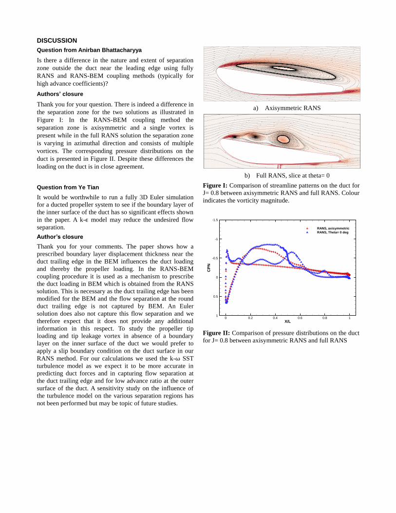
DISCUSSION

Question from Anirban Bhattacharyya

Is there a difference in the nature and extent of separation

zone outside the duct near the leading edge using fully

RANS and RANS-BEM coupling methods (typically for

high advance coefficients)?

Authors’ closure

Thank you for your question. There is indeed a difference in

the separation zone for the two solutions as illustrated in

Figure I: In the RANS-BEM coupling method the

separation zone is axisymmetric and a single vortex is

present while in the full RANS solution the separation zone

is varying in azimuthal direction and consists of multiple

vortices. The corresponding pressure distributions on the

duct is presented in Figure II. Despite these differences the

loading on the duct is in close agreement.

Question from Ye Tian

It would be worthwhile to run a fully 3D Euler simulation

for a ducted propeller system to see if the boundary layer of

the inner surface of the duct has so significant effects shown

in the paper. A k-ϵ model may reduce the undesired flow

separation.

Author’s closure

Thank you for your comments. The paper shows how a

prescribed boundary layer displacement thickness near the

duct trailing edge in the BEM influences the duct loading

and thereby the propeller loading. In the RANS-BEM

coupling procedure it is used as a mechanism to prescribe

the duct loading in BEM which is obtained from the RANS

solution. This is necessary as the duct trailing edge has been

modified for the BEM and the flow separation at the round

duct trailing edge is not captured by BEM. An Euler

solution does also not capture this flow separation and we

therefore expect that it does not provide any additional

information in this respect. To study the propeller tip

loading and tip leakage vortex in absence of a boundary

layer on the inner surface of the duct we would prefer to

apply a slip boundary condition on the duct surface in our

RANS method. For our calculations we used the k-ω SST

turbulence model as we expect it to be more accurate in

predicting duct forces and in capturing flow separation at

the duct trailing edge and for low advance ratio at the outer

surface of the duct. A sensitivity study on the influence of

the turbulence model on the various separation regions has

not been performed but may be topic of future studies.

a) Axisymmetric RANS

b) Full RANS, slice at theta= 0

Figure I: Comparison of streamline patterns on the duct for

J= 0.8 between axisymmetric RANS and full RANS. Colour

indicates the vorticity magnitude.

Figure II: Comparison of pressure distributions on the duct

for J= 0.8 between axisymmetric RANS and full RANS

++++++

++++++++++

+++++ +++++ +++++ +++++ ++++++++++

+++++++++++++++++

+++++++++++++++++++

+++++

++++

+++++

+++++

+

+

+++

++++++ +++++ +++++ +++++ +++++ +++++ +++++ +++++ +++++ +++++ +++++ +++++ +++++ +++++++++++ ++++

++++++++++

+

+

+

+

+

++++

++++

X/L

CP

N

0 0.2 0.4 0.6 0.8 1

-1.5

-1

-0.5

0

0.5

1

RANS, axisymmetric

RANS, Theta= 0 deg+