Analysis of Count Data Chapter 14 Goodness of fit Formulas and models for two-way

tables- tests for independence- tests of homogeneity

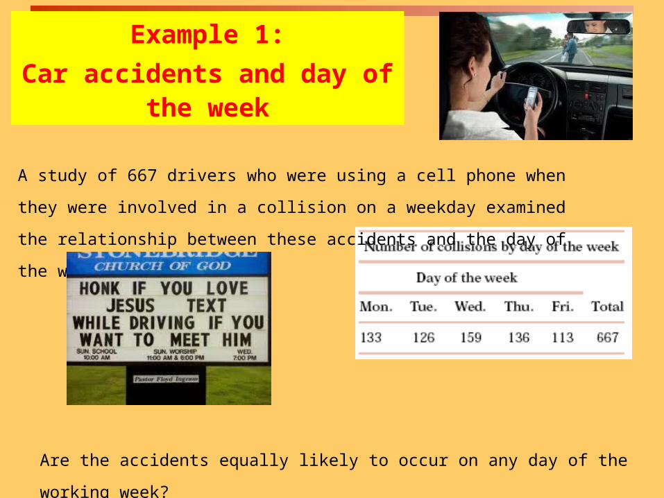
A study of 667 drivers who were using a cell phone when they were involved

in a collision on a weekday examined the relationship between these

accidents and the day of the week.

Example 1:

Car accidents and day of the week

Are the accidents equally likely to occur on any day of the working week?

Example 2: M & M Colors

Mars, Inc. periodically changes the M&M (milk chocolate) color proportions. Last year the proportions were:

yellow 20%; red 20%, orange, blue, green 10% each; brown 30% In a recent bag of 106 M&M’s I had the following numbers of each

color:

Is this evidence that Mars, Inc. has changed the color distribution of M&M’s?

Yellow Red Orange Blue Green Brown

29 (27.4%) 23 (21.7%) 12 (11.3%) 14 (13.2%) 8 (7.5%) 20 (18.9%)

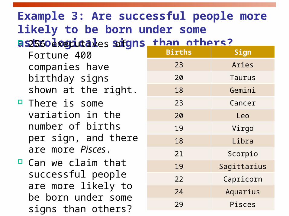
Example 3: Are successful people more likely to be born under some astrological signs than others? 256 executives of Fortune

400 companies have birthday signs shown at the right.

There is some variation in the number of births per sign, and there are more Pisces.

Can we claim that successful people are more likely to be born under some signs than others?

Births Sign

23 Aries

20 Taurus

18 Gemini

23 Cancer

20 Leo

19 Virgo

18 Libra

21 Scorpio

19 Sagittarius

22 Capricorn

24 Aquarius

29 Pisces

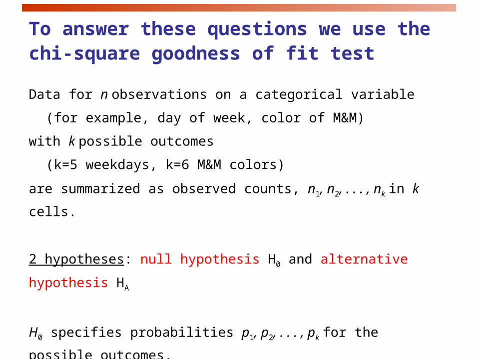
To answer these questions we use the chi-square goodness of fit test

Data for n observations on a categorical variable

(for example, day of week, color of M&M)

with k possible outcomes

(k=5 weekdays, k=6 M&M colors)

are summarized as observed counts, n1, n2, . . . , nk in k cells.

2 hypotheses: null hypothesis H0 and alternative hypothesis HA

H0 specifies probabilities p1, p2, . . . , pk for the possible outcomes.

HA states that the probabilities are different from those in H0

The Chi-Square Test StatisticThe Chi-square test statistic is:

22

cells

( )

all

Obs Exp

Exp

where: Obs = observed frequency in a particular cell Exp= expected frequency in a particular cell if H0 is true

The expected frequency in cell i is npi

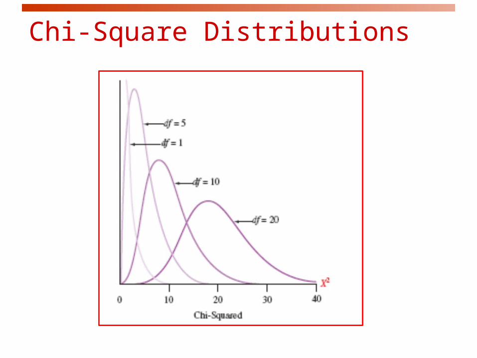
Chi-Square Distributions

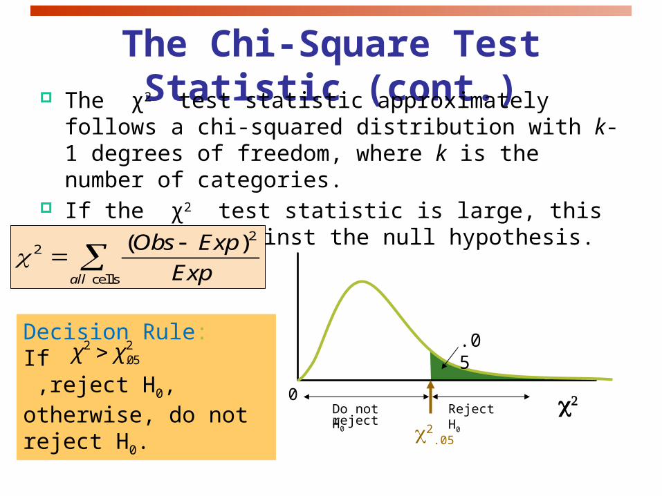
The Chi-Square Test Statistic (cont.) The χ2 test statistic approximately follows a chi-squared

distribution with k-1 degrees of freedom, where k is the number of categories.

If the χ2 test statistic is large, this is evidence against the null hypothesis.

Decision Rule:If ,reject H0, otherwise, do not reject H0.

2 2.05χ χ

22

.05

0

.05

Reject H0Do not reject H0

22

cells

( )

all

Obs Exp

Exp

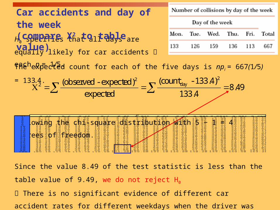
H0 specifies that all days are equally likely for

car accidents each pi = 1/5.

Car accidents and day of the week(compare X2 to table value)

The expected count for each of the five days is npi = 667(1/5) = 133.4.

Following the chi-square distribution with 5 − 1 = 4 degrees of freedom.p

df 0.25 0.2 0.15 0.1 0.05 0.025 0.02 0.01 0.005 0.0025 0.001 0.00051 1.32 1.64 2.07 2.71 3.84 5.02 5.41 6.63 7.88 9.14 10.83 12.12 2 2.77 3.22 3.79 4.61 5.99 7.38 7.82 9.21 10.60 11.98 13.82 15.20 3 4.11 4.64 5.32 6.25 7.81 9.35 9.84 11.34 12.84 14.32 16.27 17.73 4 5.39 5.99 6.74 7.78 9.49 11.14 11.67 13.28 14.86 16.42 18.47 20.00 5 6.63 7.29 8.12 9.24 11.07 12.83 13.39 15.09 16.75 18.39 20.51 22.11 6 7.84 8.56 9.45 10.64 12.59 14.45 15.03 16.81 18.55 20.25 22.46 24.10 7 9.04 9.80 10.75 12.02 14.07 16.01 16.62 18.48 20.28 22.04 24.32 26.02 8 10.22 11.03 12.03 13.36 15.51 17.53 18.17 20.09 21.95 23.77 26.12 27.87 9 11.39 12.24 13.29 14.68 16.92 19.02 19.68 21.67 23.59 25.46 27.88 29.67 10 12.55 13.44 14.53 15.99 18.31 20.48 21.16 23.21 25.19 27.11 29.59 31.42 11 13.70 14.63 15.77 17.28 19.68 21.92 22.62 24.72 26.76 28.73 31.26 33.14 12 14.85 15.81 16.99 18.55 21.03 23.34 24.05 26.22 28.30 30.32 32.91 34.82 13 15.98 16.98 18.20 19.81 22.36 24.74 25.47 27.69 29.82 31.88 34.53 36.48 14 17.12 18.15 19.41 21.06 23.68 26.12 26.87 29.14 31.32 33.43 36.12 38.11 15 18.25 19.31 20.60 22.31 25.00 27.49 28.26 30.58 32.80 34.95 37.70 39.72 16 19.37 20.47 21.79 23.54 26.30 28.85 29.63 32.00 34.27 36.46 39.25 41.31 17 20.49 21.61 22.98 24.77 27.59 30.19 31.00 33.41 35.72 37.95 40.79 42.88 18 21.60 22.76 24.16 25.99 28.87 31.53 32.35 34.81 37.16 39.42 42.31 44.43 19 22.72 23.90 25.33 27.20 30.14 32.85 33.69 36.19 38.58 40.88 43.82 45.97 20 23.83 25.04 26.50 28.41 31.41 34.17 35.02 37.57 40.00 42.34 45.31 47.50 21 24.93 26.17 27.66 29.62 32.67 35.48 36.34 38.93 41.40 43.78 46.80 49.01 22 26.04 27.30 28.82 30.81 33.92 36.78 37.66 40.29 42.80 45.20 48.27 50.51 23 27.14 28.43 29.98 32.01 35.17 38.08 38.97 41.64 44.18 46.62 49.73 52.00 24 28.24 29.55 31.13 33.20 36.42 39.36 40.27 42.98 45.56 48.03 51.18 53.48 25 29.34 30.68 32.28 34.38 37.65 40.65 41.57 44.31 46.93 49.44 52.62 54.95 26 30.43 31.79 33.43 35.56 38.89 41.92 42.86 45.64 48.29 50.83 54.05 56.41 27 31.53 32.91 34.57 36.74 40.11 43.19 44.14 46.96 49.64 52.22 55.48 57.86 28 32.62 34.03 35.71 37.92 41.34 44.46 45.42 48.28 50.99 53.59 56.89 59.30 29 33.71 35.14 36.85 39.09 42.56 45.72 46.69 49.59 52.34 54.97 58.30 60.73 30 34.80 36.25 37.99 40.26 43.77 46.98 47.96 50.89 53.67 56.33 59.70 62.16 40 45.62 47.27 49.24 51.81 55.76 59.34 60.44 63.69 66.77 69.70 73.40 76.09 50 56.33 58.16 60.35 63.17 67.50 71.42 72.61 76.15 79.49 82.66 86.66 89.56 60 66.98 68.97 71.34 74.40 79.08 83.30 84.58 88.38 91.95 95.34 99.61 102.70 80 88.13 90.41 93.11 96.58 101.90 106.60 108.10 112.30 116.30 120.10 124.80 128.30

100 109.10 111.70 114.70 118.50 124.30 129.60 131.10 135.80 140.20 144.30 149.40 153.20

22day2 (count - 133.4)(observed - expected)

8.49expected 133.4

Since the value 8.49 of the test statistic is less than the table value of 9.49, we

do not reject H0

There is no significant evidence of different car accident rates for different

weekdays when the driver was using a cell phone.

H0 specifies that all days are equally likely for car accidents each pi = 1/5.

Car accidents and day of the week(bounds on P-value)

The expected count for each of the five days is npi = 667(1/5) = 133.4.

Following the chi-square distribution with 5 − 1 = 4 degrees of freedom.p

df 0.25 0.2 0.15 0.1 0.05 0.025 0.02 0.01 0.005 0.0025 0.001 0.00051 1.32 1.64 2.07 2.71 3.84 5.02 5.41 6.63 7.88 9.14 10.83 12.12 2 2.77 3.22 3.79 4.61 5.99 7.38 7.82 9.21 10.60 11.98 13.82 15.20 3 4.11 4.64 5.32 6.25 7.81 9.35 9.84 11.34 12.84 14.32 16.27 17.73 4 5.39 5.99 6.74 7.78 9.49 11.14 11.67 13.28 14.86 16.42 18.47 20.00 5 6.63 7.29 8.12 9.24 11.07 12.83 13.39 15.09 16.75 18.39 20.51 22.11 6 7.84 8.56 9.45 10.64 12.59 14.45 15.03 16.81 18.55 20.25 22.46 24.10 7 9.04 9.80 10.75 12.02 14.07 16.01 16.62 18.48 20.28 22.04 24.32 26.02 8 10.22 11.03 12.03 13.36 15.51 17.53 18.17 20.09 21.95 23.77 26.12 27.87 9 11.39 12.24 13.29 14.68 16.92 19.02 19.68 21.67 23.59 25.46 27.88 29.67 10 12.55 13.44 14.53 15.99 18.31 20.48 21.16 23.21 25.19 27.11 29.59 31.42 11 13.70 14.63 15.77 17.28 19.68 21.92 22.62 24.72 26.76 28.73 31.26 33.14 12 14.85 15.81 16.99 18.55 21.03 23.34 24.05 26.22 28.30 30.32 32.91 34.82 13 15.98 16.98 18.20 19.81 22.36 24.74 25.47 27.69 29.82 31.88 34.53 36.48 14 17.12 18.15 19.41 21.06 23.68 26.12 26.87 29.14 31.32 33.43 36.12 38.11 15 18.25 19.31 20.60 22.31 25.00 27.49 28.26 30.58 32.80 34.95 37.70 39.72 16 19.37 20.47 21.79 23.54 26.30 28.85 29.63 32.00 34.27 36.46 39.25 41.31 17 20.49 21.61 22.98 24.77 27.59 30.19 31.00 33.41 35.72 37.95 40.79 42.88 18 21.60 22.76 24.16 25.99 28.87 31.53 32.35 34.81 37.16 39.42 42.31 44.43 19 22.72 23.90 25.33 27.20 30.14 32.85 33.69 36.19 38.58 40.88 43.82 45.97 20 23.83 25.04 26.50 28.41 31.41 34.17 35.02 37.57 40.00 42.34 45.31 47.50 21 24.93 26.17 27.66 29.62 32.67 35.48 36.34 38.93 41.40 43.78 46.80 49.01 22 26.04 27.30 28.82 30.81 33.92 36.78 37.66 40.29 42.80 45.20 48.27 50.51 23 27.14 28.43 29.98 32.01 35.17 38.08 38.97 41.64 44.18 46.62 49.73 52.00 24 28.24 29.55 31.13 33.20 36.42 39.36 40.27 42.98 45.56 48.03 51.18 53.48 25 29.34 30.68 32.28 34.38 37.65 40.65 41.57 44.31 46.93 49.44 52.62 54.95 26 30.43 31.79 33.43 35.56 38.89 41.92 42.86 45.64 48.29 50.83 54.05 56.41 27 31.53 32.91 34.57 36.74 40.11 43.19 44.14 46.96 49.64 52.22 55.48 57.86 28 32.62 34.03 35.71 37.92 41.34 44.46 45.42 48.28 50.99 53.59 56.89 59.30 29 33.71 35.14 36.85 39.09 42.56 45.72 46.69 49.59 52.34 54.97 58.30 60.73 30 34.80 36.25 37.99 40.26 43.77 46.98 47.96 50.89 53.67 56.33 59.70 62.16 40 45.62 47.27 49.24 51.81 55.76 59.34 60.44 63.69 66.77 69.70 73.40 76.09 50 56.33 58.16 60.35 63.17 67.50 71.42 72.61 76.15 79.49 82.66 86.66 89.56 60 66.98 68.97 71.34 74.40 79.08 83.30 84.58 88.38 91.95 95.34 99.61 102.70 80 88.13 90.41 93.11 96.58 101.90 106.60 108.10 112.30 116.30 120.10 124.80 128.30

100 109.10 111.70 114.70 118.50 124.30 129.60 131.10 135.80 140.20 144.30 149.40 153.20

22day2 (count - 133.4)(observed - expected)

8.49expected 133.4

There is no significant evidence of different car accident rates for different weekdays when the driver was using a cell phone.

7.78 < X2= 8.49 < 9.49 Thus the bounds on the P-value are 0.05 < P-value < 0.1

We don’t know the exact P-value but we DO know that P-value > 0.05, thus we conclude that …

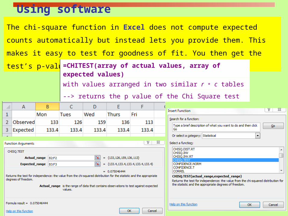
Using software

The chi-square function in Excel does not compute expected counts automatically

but instead lets you provide them. This makes it easy to test for goodness of fit. You

then get the test’s p-value—but no details of the X2 calculations.

=CHITEST(array of actual values, array of expected values)

with values arranged in two similar r * c tables

--> returns the p value of the Chi Square test

Example 2: M & M Colors

H0 : pyellow=.20, pred=.20, porange=.10, pblue=.10, pgreen=.10, pbrown=.30

Expected yellow = 106*.20 = 21.2, etc. for other expected counts.

Yellow Red Orange Blue Green Brown Total

Obs. 29 23 12 14 8 20 106

Exp. 21.2 21.2 10.6 10.6 10.6 31.8 106

2 2 22

cells

2 2 2 2

( ) (29 21.2) (23 21.2)

21.2 21.2

(12 10.6) (14 10.6) (8 10.6) (20 31.8)

10.6 10.6 10.6 31.82.87 0.153 0.185 1.091 0.638 4.379

9.316

all

Obs Exp

Exp

Example 2: M & M Colors (cont.)

2 9.316;degrees of freedom 6 1 5

2 20.05The test statistic is 9.316 ; with 5 d.f. 11.070χ χ

Decision Rule:If ,reject H0, otherwise, do not reject H0.

2 2.05χ χ

2

20.05 = 11.070

0

0.05

Reject H0Do not reject H0

Here, = 9.316 < = 11.070, so we do not reject H0 and conclude that there is not sufficient evidence to conclude that Mars has changed the color proportions.

2.05χ2χ

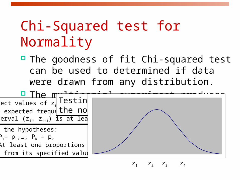
Chi-Squared test for Normality The goodness of fit Chi-squared test can be used

to determined if data were drawn from any distribution.

The multinomial experiment produces the test statistic.

z1 z2 z3 z4

Select values of zi such that the expected frequency in each interval (zi, zi+1) is at least 5.

Test the hypotheses:H0: P1= p1,…, Pk = pk

H1: At least one proportions differs from its specified value. p1

p2

p3p3

p2

p1

np2 > 5 np2 > 5

np1 > 5

np3 > 5 np3 > 5

np1 > 5

For example:P(z1<z<z2)=p2

Testing goodness of fit for the normal distribution

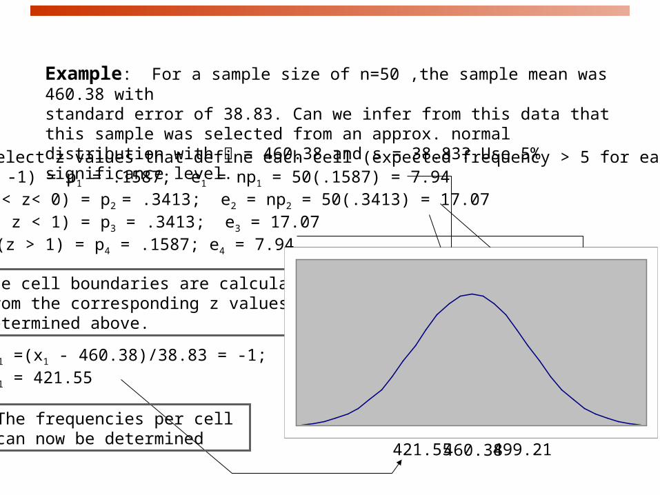
SolutionFirst let us select z values that define each cell (expected frequency > 5 for each cell.)z1 = -1; P(z < -1) = p1 = .1587; e1 = np1 = 50(.1587) = 7.94z2 = 0; P(-1 < z< 0) = p2 = .3413; e2 = np2 = 50(.3413) = 17.07z3 = 1; P(0 < z < 1) = p3 = .3413; e3 = 17.07 P(z > 1) = p4 = .1587; e4 = 7.94

421.55 460.38 499.21

p1

p2

p1

p2

The cell boundaries are calculatedfrom the corresponding z values determined above.

z1 =(x1 - 460.38)/38.83 = -1; x1 = 421.55

The frequencies per cell can now be determined

Expected frequencies

Sample frequencies

f1 = 10

f2 = 13

f3 = 19

f4 = 8

e1 = 7.94

e2 = 17.07e3 = 17.07

e4 = 7.94

Example: For a sample size of n=50 ,the sample mean was 460.38 with standard error of 38.83. Can we infer from this data that this sample was selected from an approx. normal distribution with = 460.38 and s = 38.83? Use 5% significance level.

Conclusion: There is insufficient evidence to conclude at 5% significance level that the data are not approx. normally distributed.

(10 - 7.94)2

7.94(13 - 17.07)2

17.07(19 - 17.07)2

17.072 = = 1.72+ + (8 - 7.94)2

7.94+

23,

2 k

– The rejection region

– The test statistic

84146.3234,05.

23k,

The chi-square test is an overall technique for comparing any number

of population proportions, testing for evidence of a relationship

between two categorical variables. There are 2 types of tests:

1. Test for independence: Take one SRS and classify the individuals in

the sample according to two categorical variables (attribute or condition)

observational study, historical design.

2. Compare several populations (tests for homogeneity): Randomly

select several SRSs each from a different population (or from a

population subjected to different treatments) experimental study.

Both models use the X2 test to test of the hypothesis of no relationship.

Models for two-way tables

Testing for independence

We have now a single sample from a single population. For each

individual in this SRS of size n we measure two categorical variables.

The results are then summarized in a two-way table.

The null hypothesis is that the row and column variables are

independent. The alternative hypothesis is that the row and column

variables are dependent.

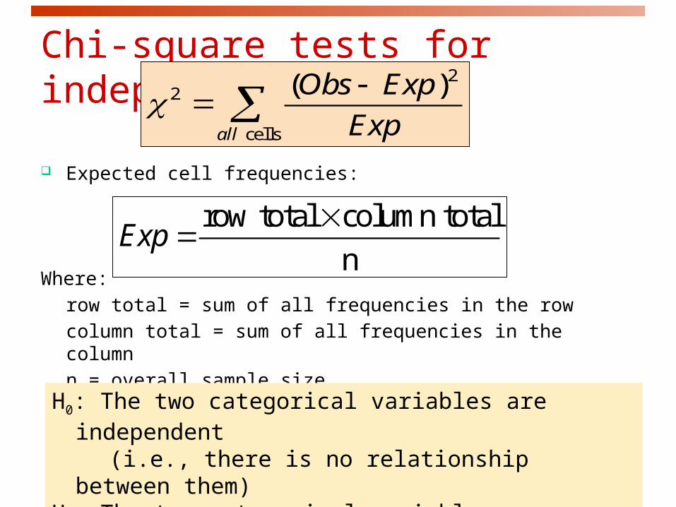
Chi-square tests for independence

Expected cell frequencies:

Where:

row total = sum of all frequencies in the row

column total = sum of all frequencies in the column

n = overall sample size

22

cells

( )

all

Obs Exp

Exp

row total column total

nExp

H0: The two categorical variables are independent(i.e., there is no relationship between them)

H1: The two categorical variables are dependent(i.e., there is a relationship between them)

Example 1: Parental smoking Does parental smoking influence the incidence of smoking in

children when they reach high school? Randomly chosen high school students were asked whether they smoked (columns) and whether their parents smoked (rows).

Are parent smoking status and student smoking status related? H0 : parent smoking status and student smoking status are

independent HA : parent smoking status and student smoking status are not

independent

Student

Smoke No smoke Total

Both smoke 400 1380 1780

Parent One smokes 416 1823 2239

Neither smokes 188 1168 1356

Total 1004 4371 5375

Example 1: Parental smoking (cont.)Does parental smoking influence the incidence of smoking in children when

they reach high school? Randomly chosen high school students were asked

whether they smoked (columns) and whether their parents smoked (rows).

Examine the computer output for the chi-square test performed on these data.

What does it tell you?

Hypotheses?Are data ok for c2 test? (All expected counts 5 or more)

df = (rows-1)*(cols-1)=2*1=2

Interpretation? Since P-value is less than .05, reject H0 and conclude that parent smoking status and student smoking status are related.

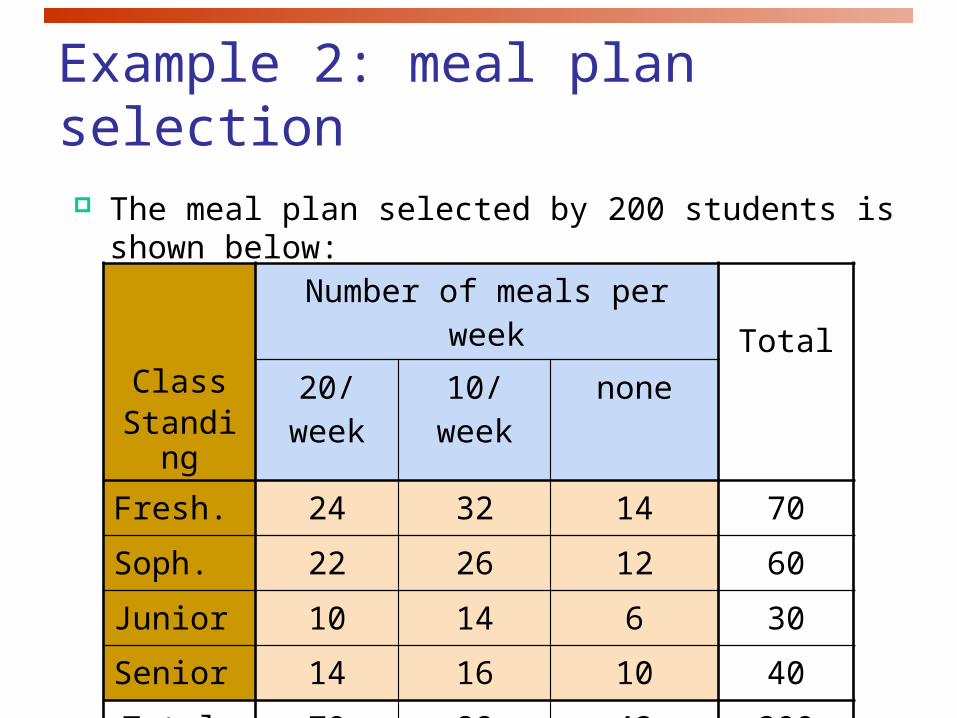
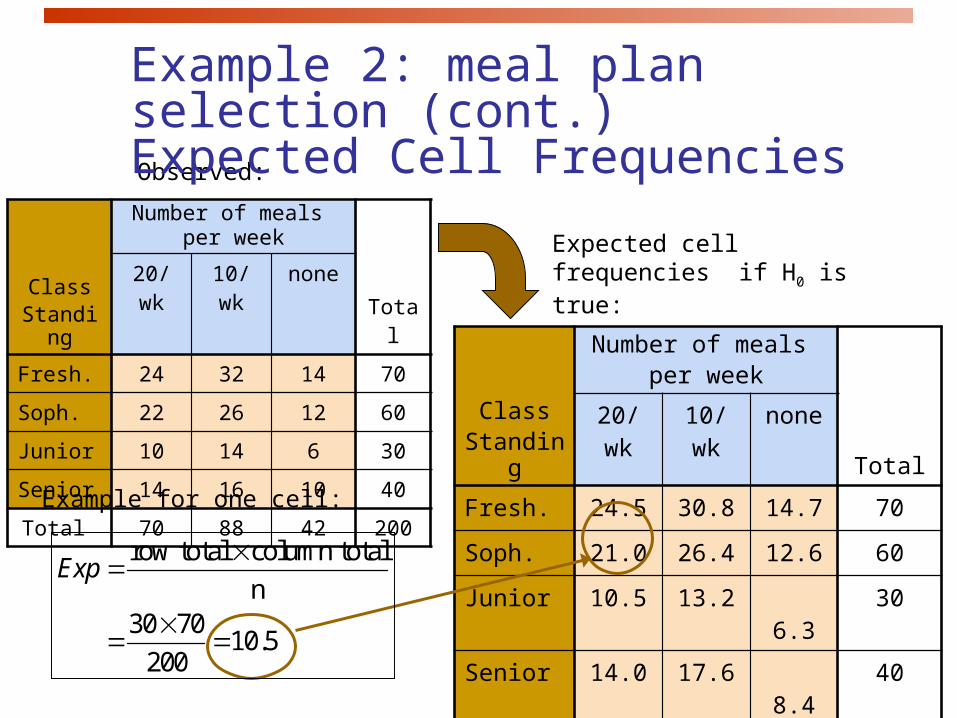
Example 2: meal plan selection

The meal plan selected by 200 students is shown below:

ClassStanding

Number of meals per weekTotal20/week 10/week none

Fresh. 24 32 14 70

Soph. 22 26 12 60

Junior 10 14 6 30

Senior 14 16 10 40

Total 70 88 42 200

Example 2: meal plan selection (cont.) The hypotheses to be tested are:

H0: Meal plan and class standing are independent

(i.e., there is no relationship between them)

H1: Meal plan and class standing are dependent

(i.e., there is a relationship between them)

ClassStanding

Number of meals per week

Total20/wk 10/wk none

Fresh. 24 32 14 70

Soph. 22 26 12 60

Junior 10 14 6 30

Senior 14 16 10 40

Total 70 88 42 200

ClassStanding

Number of meals per week

Total20/wk 10/wk none

Fresh. 24.5 30.8 14.7 70

Soph. 21.0 26.4 12.6 60

Junior 10.5 13.2 6.3 30

Senior 14.0 17.6 8.4 40

Total 70 88 42 200

Observed:

Expected cell frequencies if H0 is true:

row total column total

n30 70

10.5200

Exp

Example for one cell:

Example 2: meal plan selection (cont.) Expected Cell Frequencies

Example 2: meal plan selection (cont.) The Test Statistic The test statistic value is:

22

cells

2 2 2

( )

(24 24.5) (32 30.8) (10 8.4)0.709

24.5 30.8 8.4

all

Obs Exp

Exp

= 12.592 from the chi-squared distribution with (4 – 1)(3 – 1) = 6 degrees of freedom

2050.

χ

Example 2: meal plan selection (cont.) Decision and Interpretation

Decision Rule:If > 12.592, reject H0, otherwise, do not reject H0

2 20.05The test statistic is 0.709 ; with 6 d.f. 12.592

Here, = 0.709 < = 12.592, so do not reject H0 Conclusion: there is not sufficient evidence that meal plan and class standing are related.

2

20.05=12.592

0

0.05

Reject H0Do not reject H0

2

2 2050.

χ

The chi-square test is an overall technique for comparing any number of population proportions, testing for evidence of a relationship between two categorical variables. There are 2 types of tests:

1. Test for independence: Take one SRS and classify the individuals in the

sample according to two categorical variables (attribute or condition)

observational study, historical design.

NEXT:

Models for two-way tables

2. Compare several populations (tests for homogeneity): Randomly

select several SRSs each from a different population (or from a population

subjected to different treatments) experimental study.

Both models use the X2 test to test of the hypothesis of no relationship.

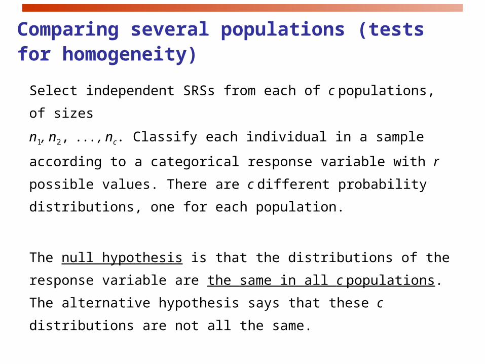
Comparing several populations (tests for homogeneity)

Select independent SRSs from each of c populations, of sizes

n1, n2, . . . , nc. Classify each individual in a sample according to a

categorical response variable with r possible values. There are c

different probability distributions, one for each population.

The null hypothesis is that the distributions of the response variable are

the same in all c populations. The alternative hypothesis says that

these c distributions are not all the same.

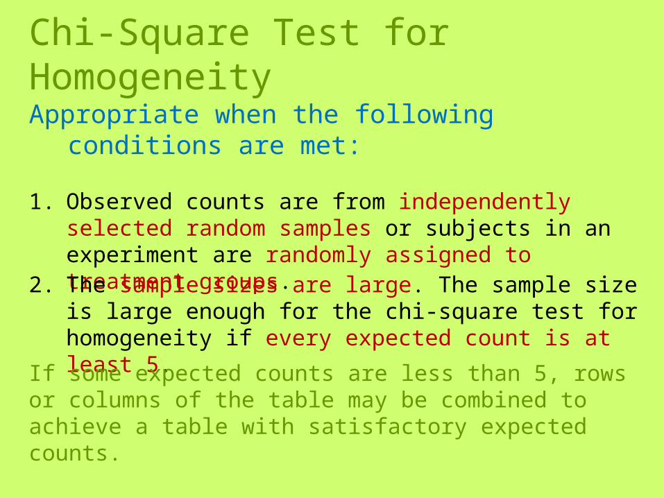
Chi-Square Test for Homogeneity

Appropriate when the following conditions are met:

1. Observed counts are from independently selected random samples or subjects in an experiment are randomly assigned to treatment groups.

2. The sample sizes are large. The sample size is large enough for the chi-square test for homogeneity if every expected count is at least 5.

If some expected counts are less than 5, rows or columns of the table may be combined to achieve a table with satisfactory expected counts.

•  

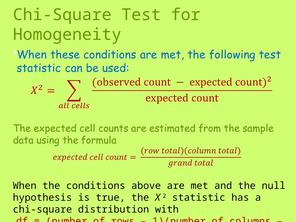
Chi-Square Test for Homogeneity

 

When the conditions above are met and the null hypothesis is true, the X 2 statistic has a chi-square distribution with

df = (number of rows – 1)(number of columns – 1)

Associated P-value: The P-value associated with the computed test statistic value is the area to the right of X 2 under the chi-square curve withdf = (no. of rows – 1)(no. of cols. – 1)

Hypothesis:

H0: the population (or treatment) category proportions are the same for all the populations (or treatments)

Ha: the population (or treatment) category proportions are not all the same for all the populations (or treatments)

Chi-Square Test for Homogeneity

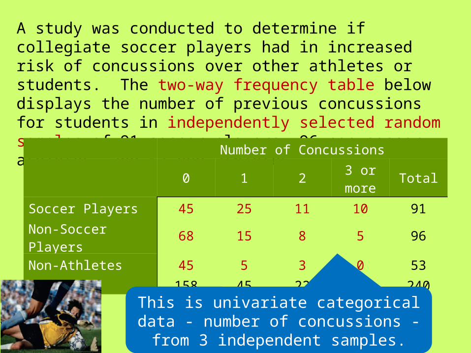
A study was conducted to determine if collegiate soccer players had in increased risk of concussions over other athletes or students. The two-way frequency table below displays the number of previous concussions for students in independently selected random samples of 91 soccer players, 96 non-soccer athletes, and 53 non-athletes.Number of Concussions

0 1 2 3 or more

Total

Soccer Players 45 25 11 10 91

Non-Soccer Players 68 15 8 5 96

Non-Athletes 45 5 3 0 53

Total 158 45 22 15 240

This is univariate categorical data - number of concussions - from 3

independent samples.

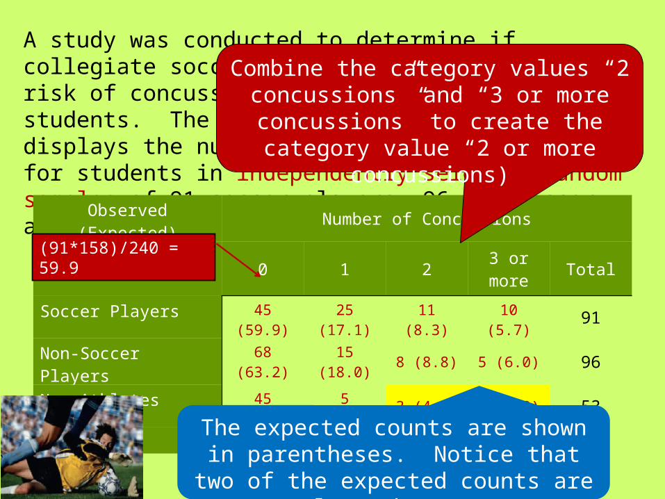
A study was conducted to determine if collegiate soccer players had in increased risk of concussions over other athletes or students. The two-way frequency table below displays the number of previous concussions for students in independently selected random samples of 91 soccer players, 96 non-soccer athletes, and 53 non-athletes.Observed

(Expected) Number of Concussions

0 1 2 3 or more Total

Soccer Players 45 (59.9) 25 (17.1) 11 (8.3) 10 (5.7) 91

Non-Soccer Players 68 (63.2) 15 (18.0) 8 (8.8) 5 (6.0) 96

Non-Athletes 45 (34.9) 5 (10.0) 3 (4.9) 0 (3.3) 53

Total 158 45 22 15 240

The expected counts are shown in parentheses. Notice that two of the

expected counts are less than 5.

Combine the category values “2 concussions” and “3 or more

concussions” to create the category value “2 or more concussions)

(91*158)/240 = 59.9

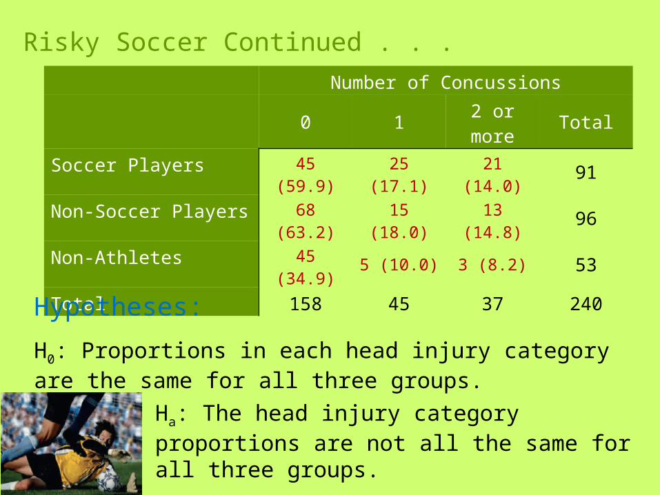
Risky Soccer Continued . . .Number of Concussions

0 1 2 or more

Total

Soccer Players 45 (59.9) 25 (17.1) 21 (14.0) 91

Non-Soccer Players 68 (63.2) 15 (18.0) 13 (14.8) 96

Non-Athletes 45 (34.9) 5 (10.0) 3 (8.2) 53

Total 158 45 37 240

Hypotheses:

H0: Proportions in each head injury category are the same for all three groups.

Ha: The head injury category proportions are not all the same for all three groups.

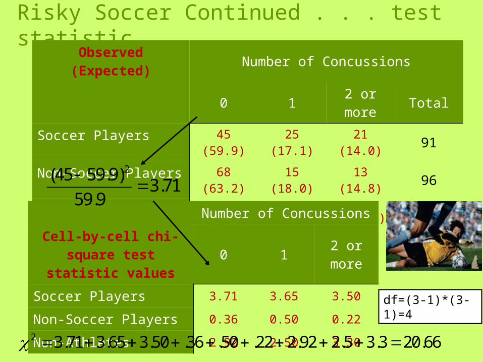
Risky Soccer Continued . . . test statisticObserved

(Expected) Number of Concussions

0 1 2 or more

Total

Soccer Players 45 (59.9) 25 (17.1) 21 (14.0) 91

Non-Soccer Players 68 (63.2) 15 (18.0) 13 (14.8) 96

Non-Athletes 45 (34.9) 5 (10.0) 3 (8.2) 53

Total 158 45 37 240

Number of Concussions

Cell-by-cell chi-square test statistic

values0 1 2 or

more

Soccer Players 3.71 3.65 3.50

Non-Soccer Players 0.36 0.50 0.22

Non-Athletes 2.92 2.50 3.30

2(45 59.9)3.71

59.9

2 3.71 3.65 3.50 .36 .50 .22 2.92 2.5 3.3 20.66

df=(3-1)*(3-1)=4

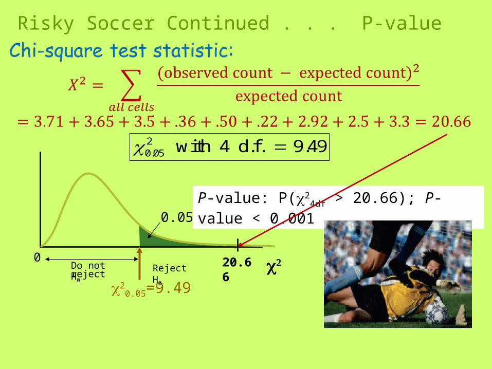
Risky Soccer Continued . . . P-value 

P-value: P(24df > 20.66); P-value <

0.001

20.05 with 4 d.f. 9.49

2

20.05=9.49

0

0.05

Reject H0Do not reject H0

20.66

Risky Soccer Continued . . . Conclusion

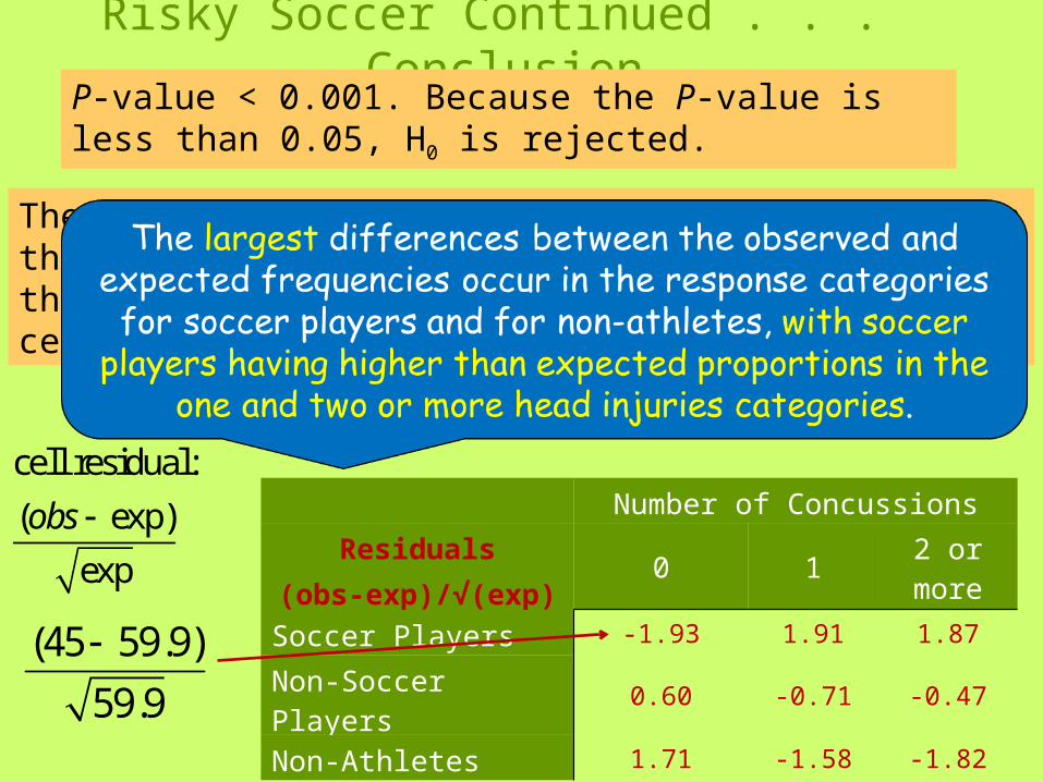
P-value < 0.001. Because the P-value is less than 0.05, H0 is rejected.

There is strong evidence that the proportions in the head injury categories are not the same for the three groups. How do they differ? Check cell residuals.

Number of Concussions

Residuals(obs-exp)/√(exp)

0 1 2 or more

Soccer Players -1.93 1.91 1.87

Non-Soccer Players 0.60 -0.71 -0.47

Non-Athletes 1.71 -1.58 -1.82

cell residual:

( exp)

exp

obs

(45 59.9)

59.9

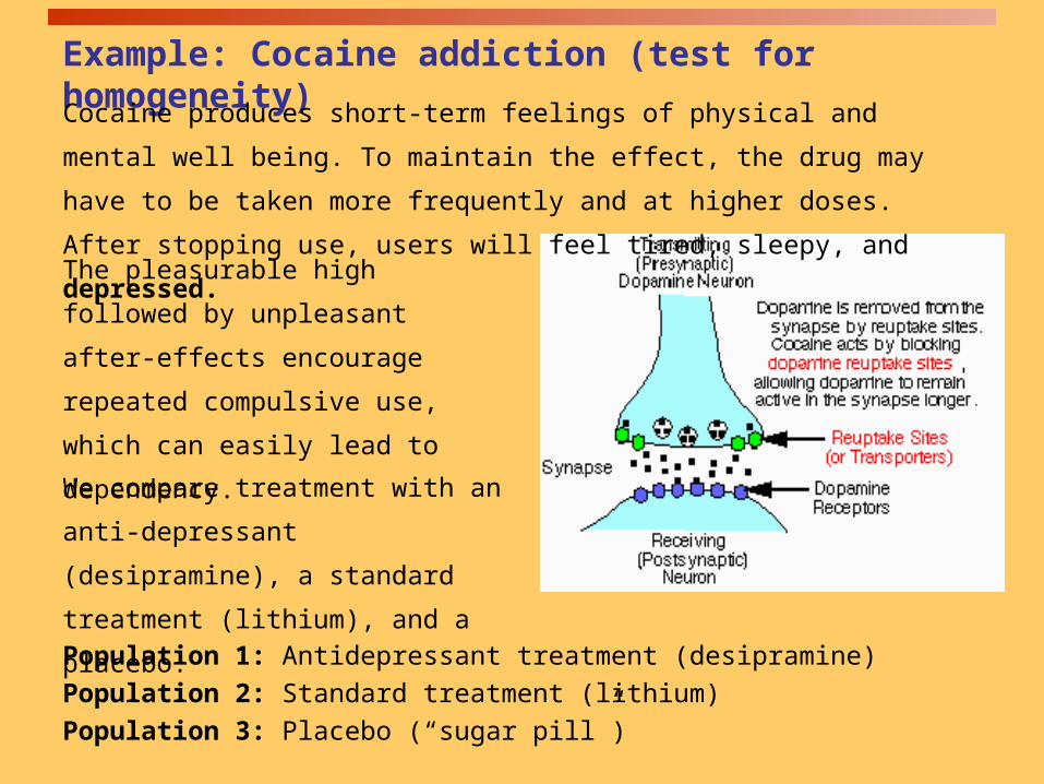
Example: Cocaine addiction (test for homogeneity)Cocaine produces short-term feelings of physical and mental well being. To

maintain the effect, the drug may have to be taken more frequently and at

higher doses. After stopping use, users will feel tired, sleepy, and depressed. 

The pleasurable high followed by

unpleasant after-effects encourage

repeated compulsive use, which can

easily lead to dependency. 

Population 1: Antidepressant treatment (desipramine)

Population 2: Standard treatment (lithium)

Population 3: Placebo (“sugar pill”)

We compare treatment with an anti-

depressant (desipramine), a standard

treatment (lithium), and a placebo.

25*26/74 ≈ 8.7825*0.35

16.2225*0.65

9.1426*0.35

16.8625*0.65

8.0823*0.35

14.9225*0.65

Desipramine

Lithium

Placebo

Expected relapse countsNo Yes

35% 35%35%

Expected

Observed

Cocaine addiction

H0: The proportions of success (no relapse)

are the same in all three populations.

Cocaine addiction

74.1092.14

92.1419

08.8

08.84

86.16

86.1619

14.9

14.97

22.16

22.1610

78.8

78.815

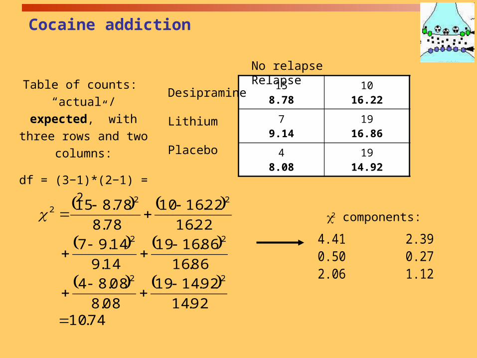
22

22

222

158.78

1016.22

79.14

1916.86

48.08

1914.92

Desipramine

Lithium

Placebo

No relapse Relapse

4.41 2.39 0.50 0.27 2.06 1.12

c2 components:

Table of counts:

“actual / expected,” with

three rows and two

columns:

df = (3−1)*(2−1) = 2

pdf 0.25 0.2 0.15 0.1 0.05 0.025 0.02 0.01 0.005 0.0025 0.001 0.00051 1.32 1.64 2.07 2.71 3.84 5.02 5.41 6.63 7.88 9.14 10.83 12.12 2 2.77 3.22 3.79 4.61 5.99 7.38 7.82 9.21 10.60 11.98 13.82 15.20 3 4.11 4.64 5.32 6.25 7.81 9.35 9.84 11.34 12.84 14.32 16.27 17.73 4 5.39 5.99 6.74 7.78 9.49 11.14 11.67 13.28 14.86 16.42 18.47 20.00 5 6.63 7.29 8.12 9.24 11.07 12.83 13.39 15.09 16.75 18.39 20.51 22.11 6 7.84 8.56 9.45 10.64 12.59 14.45 15.03 16.81 18.55 20.25 22.46 24.10 7 9.04 9.80 10.75 12.02 14.07 16.01 16.62 18.48 20.28 22.04 24.32 26.02 8 10.22 11.03 12.03 13.36 15.51 17.53 18.17 20.09 21.95 23.77 26.12 27.87 9 11.39 12.24 13.29 14.68 16.92 19.02 19.68 21.67 23.59 25.46 27.88 29.67 10 12.55 13.44 14.53 15.99 18.31 20.48 21.16 23.21 25.19 27.11 29.59 31.42 11 13.70 14.63 15.77 17.28 19.68 21.92 22.62 24.72 26.76 28.73 31.26 33.14 12 14.85 15.81 16.99 18.55 21.03 23.34 24.05 26.22 28.30 30.32 32.91 34.82 13 15.98 16.98 18.20 19.81 22.36 24.74 25.47 27.69 29.82 31.88 34.53 36.48 14 17.12 18.15 19.41 21.06 23.68 26.12 26.87 29.14 31.32 33.43 36.12 38.11 15 18.25 19.31 20.60 22.31 25.00 27.49 28.26 30.58 32.80 34.95 37.70 39.72 16 19.37 20.47 21.79 23.54 26.30 28.85 29.63 32.00 34.27 36.46 39.25 41.31 17 20.49 21.61 22.98 24.77 27.59 30.19 31.00 33.41 35.72 37.95 40.79 42.88 18 21.60 22.76 24.16 25.99 28.87 31.53 32.35 34.81 37.16 39.42 42.31 44.43 19 22.72 23.90 25.33 27.20 30.14 32.85 33.69 36.19 38.58 40.88 43.82 45.97 20 23.83 25.04 26.50 28.41 31.41 34.17 35.02 37.57 40.00 42.34 45.31 47.50 21 24.93 26.17 27.66 29.62 32.67 35.48 36.34 38.93 41.40 43.78 46.80 49.01 22 26.04 27.30 28.82 30.81 33.92 36.78 37.66 40.29 42.80 45.20 48.27 50.51 23 27.14 28.43 29.98 32.01 35.17 38.08 38.97 41.64 44.18 46.62 49.73 52.00 24 28.24 29.55 31.13 33.20 36.42 39.36 40.27 42.98 45.56 48.03 51.18 53.48 25 29.34 30.68 32.28 34.38 37.65 40.65 41.57 44.31 46.93 49.44 52.62 54.95 26 30.43 31.79 33.43 35.56 38.89 41.92 42.86 45.64 48.29 50.83 54.05 56.41 27 31.53 32.91 34.57 36.74 40.11 43.19 44.14 46.96 49.64 52.22 55.48 57.86 28 32.62 34.03 35.71 37.92 41.34 44.46 45.42 48.28 50.99 53.59 56.89 59.30 29 33.71 35.14 36.85 39.09 42.56 45.72 46.69 49.59 52.34 54.97 58.30 60.73 30 34.80 36.25 37.99 40.26 43.77 46.98 47.96 50.89 53.67 56.33 59.70 62.16 40 45.62 47.27 49.24 51.81 55.76 59.34 60.44 63.69 66.77 69.70 73.40 76.09 50 56.33 58.16 60.35 63.17 67.50 71.42 72.61 76.15 79.49 82.66 86.66 89.56 60 66.98 68.97 71.34 74.40 79.08 83.30 84.58 88.38 91.95 95.34 99.61 102.70 80 88.13 90.41 93.11 96.58 101.90 106.60 108.10 112.30 116.30 120.10 124.80 128.30 100 109.10 111.70 114.70 118.50 124.30 129.60 131.10 135.80 140.20 144.30 149.40 153.20

Cocaine addiction: Table χ

X2 = 10.71 > 5.99; df = 2

reject the H0

H0: The proportions of success (no relapse)

are the same in all three populations.

ObservedThe proportions of success are not the same in

all three populations (Desipramine, Lithium,

Placebo).

Desipramine is a more successful treatment

Avoid These Common Mistakes

Avoid These Common Mistakes

1. Don’t confuse tests for homogeneity with tests for independence. The hypotheses and conclusions are different for the two types of test.

Tests for homogeneity are used when the individuals in each of two or more independent samples are classified according to a single categorical variable.

Tests for independence are used when individuals in a single sample are classified according to two categorical variables.

Avoid These Common Mistakes

2. Remember that a hypothesis test can never show strong support for the null hypothesis.

For example, if you do not reject the null hypothesis in a chi-square test for independence, you cannot conclude that there is convincing evidence that the variables are independent. You can only say that you were not convinced that there is an association between the variables.

Avoid These Common Mistakes

3. Be sure that the conditions for the chi-square test are met.

P-values based on the chi-square distribution are only approximate, and if the large sample condition is not met, the actual P-value may be quite different from the approximate one based on the chi-square distribution.

Also, for the chi-square test of homogeneity, the assumption of independent samples is particularly important.

Avoid These Common Mistakes

4. Don’t jump to conclusions about causation. Just as a strong correlation between two numerical variables does not mean that there is a cause-and-effect relationship between them, an association between two categorical variables does not imply a causal relationship.