analysis of composite plates by using mechanics of
TRANSCRIPT
Purdue UniversityPurdue e-Pubs
Open Access Theses Theses and Dissertations
12-2016
Analysis of composite plates by using mechanics ofstructure genome and comparison with ANSYSBanghua ZhaoPurdue University
Follow this and additional works at: https://docs.lib.purdue.edu/open_access_theses
Part of the Aerospace Engineering Commons, and the Applied Mechanics Commons
This document has been made available through Purdue e-Pubs, a service of the Purdue University Libraries. Please contact [email protected] foradditional information.
Recommended CitationZhao, Banghua, "Analysis of composite plates by using mechanics of structure genome and comparison with ANSYS" (2016). OpenAccess Theses. 914.https://docs.lib.purdue.edu/open_access_theses/914

Graduate School Form 30 Updated 12/26/2015
PURDUE UNIVERSITY GRADUATE SCHOOL
Thesis/Dissertation Acceptance
This is to certify that the thesis/dissertation prepared
By
Entitled
For the degree of
Is approved by the final examining committee:
To the best of my knowledge and as understood by the student in the Thesis/Dissertation Agreement, Publication Delay, and Certification Disclaimer (Graduate School Form 32), this thesis/dissertation adheres to the provisions of Purdue University’s “Policy of Integrity in Research” and the use of copyright material.
Approved by Major Professor(s):
Approved by: Head of the Departmental Graduate Program Date
Banghua Zhao
ANALYSIS OF COMPOSITE PLATES BY USING MECHANICS OF STRUCTURE GENOME AND COMPARISON WITH ANSYS
Master of Science in Aeronautics and Astronautics
Wenbin YuChair
Tyler N. Tallman
Vikas Tomar
Wenbin Yu
Weinong Wayne Chen 12/2/2016

ANALYSIS OF COMPOSITE PLATES BY USING MECHANICS OF
STRUCTURE GENOME AND COMPARISON WITH ANSYS
A Dissertation
Submitted to the Faculty
of
Purdue University
by
Banghua Zhao
In Partial Fulfillment of the
Requirements for the Degree
of
Master of Science in Aeronautics and Astronautics
December 2016
Purdue University
West Lafayette, Indiana

ii
ACKNOWLEDGMENTS
First, I would like to thank my advisor Professor Wenbin Yu, who gave me the
opportunity to join his group to do research and work with other group members. I
learned a lot under his patient guidance and supervision. His teaching and research
philosophy have a positive influence on my graduate study and career.
I would also like to thank my committee members, Professor Vikas Tomar and
Professor Tyler Tallman, who have taken time from their busy schedule to attend my
defense and have given variable suggestions to my thesis.
I would like to thank all the group members in Professor Wenbin Yu’s group, who
were always willing to help me when I was in trouble. I gained a lot of knowledge
and experience by communication and interacting with them.
Last but not least, I would give thanks to my parents, who funded me to study
abroad in America. Their endless love always cheers me up during my hard time.
iii
TABLE OF CONTENTS
Page
LIST OF TABLES . . . . . . . . . . . . . . . . . . . . . . . . . . . . . . . . v
LIST OF FIGURES . . . . . . . . . . . . . . . . . . . . . . . . . . . . . . . vi
ABSTRACT . . . . . . . . . . . . . . . . . . . . . . . . . . . . . . . . . . . ix
1 INTRODUCTION . . . . . . . . . . . . . . . . . . . . . . . . . . . . . . 11.1 Motivation . . . . . . . . . . . . . . . . . . . . . . . . . . . . . . . . 11.2 Lecture Review . . . . . . . . . . . . . . . . . . . . . . . . . . . . . 2
1.2.1 Equivalent Single Layer Plate Theories . . . . . . . . . . . . 21.2.2 Analysis of Composite Plates by ANSYS . . . . . . . . . . . 41.2.3 Present Work and Outline . . . . . . . . . . . . . . . . . . . 7
2 MECHANICS OF STRUCTURE GENOME . . . . . . . . . . . . . . . . 92.1 Introduction . . . . . . . . . . . . . . . . . . . . . . . . . . . . . . . 92.2 SG for 3D Structures . . . . . . . . . . . . . . . . . . . . . . . . . . 102.3 SG for Plates/Shells . . . . . . . . . . . . . . . . . . . . . . . . . . 122.4 SG for Beams . . . . . . . . . . . . . . . . . . . . . . . . . . . . . . 132.5 MSG-based Multiscale Structural Modeling . . . . . . . . . . . . . . 14
3 EQUIVALENT SINGLE LAYER PLATE THEORIES . . . . . . . . . . 173.1 First Order Shear Deformation Theory . . . . . . . . . . . . . . . . 18
3.1.1 Kinematics . . . . . . . . . . . . . . . . . . . . . . . . . . . 183.1.2 Constitutive Relations . . . . . . . . . . . . . . . . . . . . . 193.1.3 Equilibrium Equations . . . . . . . . . . . . . . . . . . . . . 233.1.4 Limitations . . . . . . . . . . . . . . . . . . . . . . . . . . . 26
3.2 The Reissner-Mindlin Plate Model Based on VAM . . . . . . . . . . 273.2.1 3D Formulation . . . . . . . . . . . . . . . . . . . . . . . . . 273.2.2 Dimensional Reduction . . . . . . . . . . . . . . . . . . . . . 303.2.3 Transformation to the Reissner-Mindlin Model . . . . . . . . 373.2.4 Advantages . . . . . . . . . . . . . . . . . . . . . . . . . . . 39
4 NUMERICAL EXAMPLES . . . . . . . . . . . . . . . . . . . . . . . . . 414.1 Case 1: A 6-layer Symmetric Thin Laminate . . . . . . . . . . . . . 434.2 Case 2: A 8-layer Unsymmetrical Thick Laminate . . . . . . . . . . 504.3 Case 3: A Kiteboard . . . . . . . . . . . . . . . . . . . . . . . . . . 564.4 Case 4: A Roof Sandwich Panel . . . . . . . . . . . . . . . . . . . . 634.5 Case 5: A Corrugated-core Sandwich Panel . . . . . . . . . . . . . . 69
iv
Page
5 SUMMARY . . . . . . . . . . . . . . . . . . . . . . . . . . . . . . . . . . 75
LIST OF REFERENCES . . . . . . . . . . . . . . . . . . . . . . . . . . . . 77
A CALCULATION OF SHEAR CORRECTION FACTORS . . . . . . . . 79
B ANSYS-SWIFTCOMP GUI . . . . . . . . . . . . . . . . . . . . . . . . . 83B.1 ANSYS-SwiftComp GUI Overview . . . . . . . . . . . . . . . . . . 83B.2 Create Common SGs . . . . . . . . . . . . . . . . . . . . . . . . . . 85B.3 Homogenization and Dehomogenization . . . . . . . . . . . . . . . . 87
v
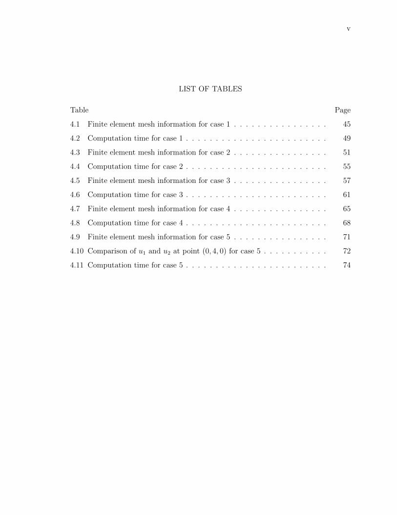
LIST OF TABLES
Table Page
4.1 Finite element mesh information for case 1 . . . . . . . . . . . . . . . . 45
4.2 Computation time for case 1 . . . . . . . . . . . . . . . . . . . . . . . . 49
4.3 Finite element mesh information for case 2 . . . . . . . . . . . . . . . . 51
4.4 Computation time for case 2 . . . . . . . . . . . . . . . . . . . . . . . . 55
4.5 Finite element mesh information for case 3 . . . . . . . . . . . . . . . . 57
4.6 Computation time for case 3 . . . . . . . . . . . . . . . . . . . . . . . . 61
4.7 Finite element mesh information for case 4 . . . . . . . . . . . . . . . . 65
4.8 Computation time for case 4 . . . . . . . . . . . . . . . . . . . . . . . . 68
4.9 Finite element mesh information for case 5 . . . . . . . . . . . . . . . . 71
4.10 Comparison of u1 and u2 at point (0, 4, 0) for case 5 . . . . . . . . . . . 72
4.11 Computation time for case 5 . . . . . . . . . . . . . . . . . . . . . . . . 74

vi
LIST OF FIGURES
Figure Page
1.1 ANSYS Composite PrepPost . . . . . . . . . . . . . . . . . . . . . . . . 6
2.1 Typical structure components . . . . . . . . . . . . . . . . . . . . . . . 10
2.2 SG for 3D structures . . . . . . . . . . . . . . . . . . . . . . . . . . . . 11
2.3 SG for Plates/Shells . . . . . . . . . . . . . . . . . . . . . . . . . . . . 13
2.4 SG for Beams . . . . . . . . . . . . . . . . . . . . . . . . . . . . . . . . 14
2.5 Work flow of Mechanics of Structure Genome . . . . . . . . . . . . . . 15
3.1 Sign convention for the displacements and rotation of a laminate . . . . 17
3.2 Plate reference surface slope and transverse normal . . . . . . . . . . . 18
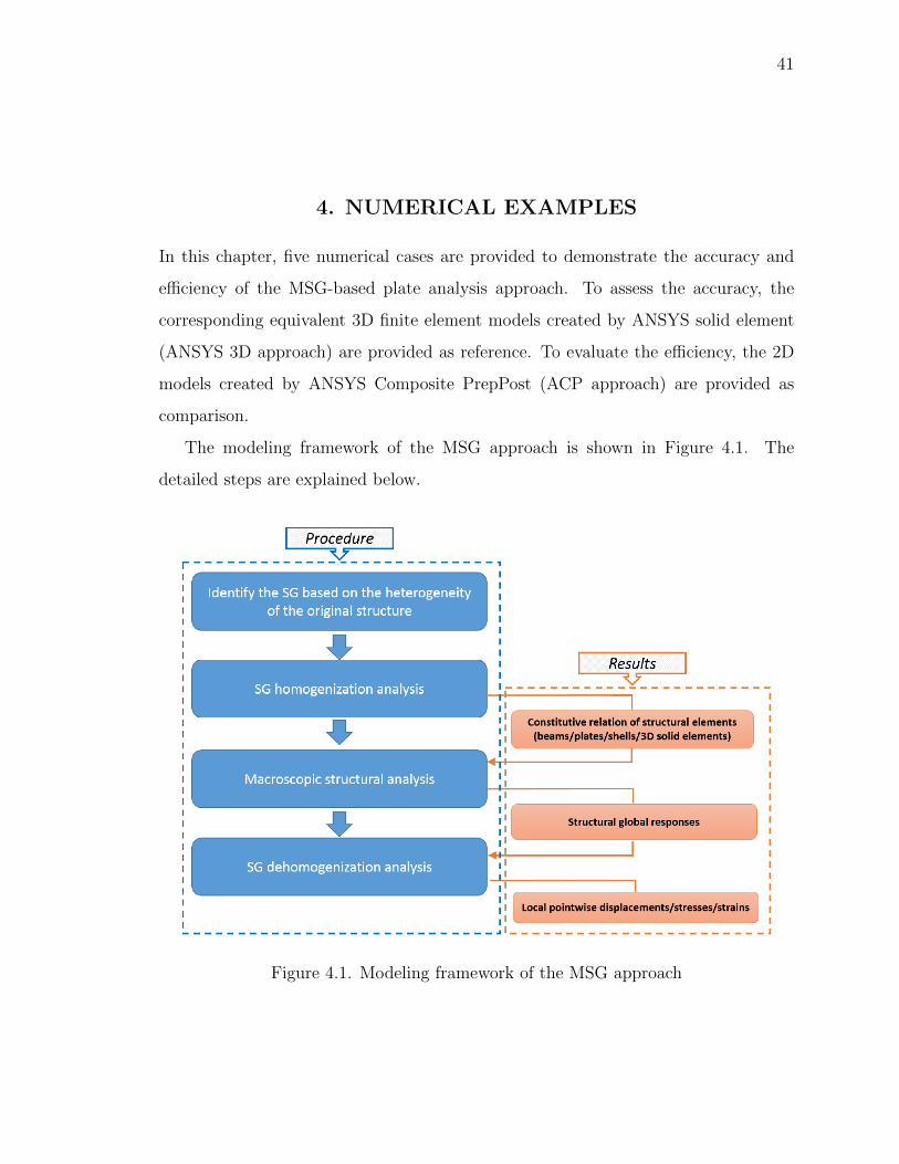
4.1 Modeling framework of the MSG approach . . . . . . . . . . . . . . . . 41
4.2 Geometry and boundary condition for case 1 . . . . . . . . . . . . . . . 43
4.3 Comparison of deflection u3 along x1 at x2 = x3 = 0 for case 1 . . . . . 45
4.4 Comparison of stress σ11 through thickness for case 1 . . . . . . . . . . 46
4.5 Comparison of stress σ22 through thickness for case 1 . . . . . . . . . . 46
4.6 Comparison of stress σ12 through thickness for case 1 . . . . . . . . . . 47
4.7 Comparison of stress σ13 through thickness for case 1 . . . . . . . . . . 47
4.8 Comparison of stress σ23 through thickness for case 1 . . . . . . . . . . 48
4.9 Comparison of stress σ33 through thickness for case 1 . . . . . . . . . . 48
4.10 Geometry and boundary condition for case 2 . . . . . . . . . . . . . . . 50
4.11 Comparison of deflection u3 along x1 at x2 = x3 = 0 for case 2 . . . . . 51
4.12 Comparison of stress σ11 through thickness for case 2 . . . . . . . . . . 52
4.13 Comparison of stress σ22 through thickness for case 2 . . . . . . . . . . 52
4.14 Comparison of stress σ12 through thickness for case 2 . . . . . . . . . . 53
4.15 Comparison of stress σ13 through thickness for case 2 . . . . . . . . . . 53
4.16 Comparison of stress σ23 through thickness for case 2 . . . . . . . . . . 54

vii
Figure Page
4.17 Comparison of stress σ33 through thickness for case 2 . . . . . . . . . . 54
4.18 Geometry and boundary condition for case 3 . . . . . . . . . . . . . . . 56
4.19 ANSYS 3D model for case 3 . . . . . . . . . . . . . . . . . . . . . . . . 57
4.20 Comparison of deflection u2 along x1 at x2 = x3 = 0 for case 3 . . . . . 58
4.21 Comparison of stress σ11 through thickness for case 3 . . . . . . . . . . 58
4.22 Comparison of stress σ22 through thickness for case 3 . . . . . . . . . . 59
4.23 Comparison of stress σ12 through thickness for case 3 . . . . . . . . . . 59
4.24 Comparison of stress σ13 through thickness for case 3 . . . . . . . . . . 60
4.25 Comparison of stress σ23 through thickness for case 3 . . . . . . . . . . 60
4.26 Comparison of stress σ33 through thickness for case 3 . . . . . . . . . . 61
4.27 Application of roof sandwich panels . . . . . . . . . . . . . . . . . . . . 63
4.28 Geometry and boundary condition for case 4 . . . . . . . . . . . . . . . 64
4.29 2D SG for roof sandwich panel . . . . . . . . . . . . . . . . . . . . . . 64
4.30 ANSYS 3D model case 4 . . . . . . . . . . . . . . . . . . . . . . . . . . 65
4.31 Comparison of deflection u2 along x2 = 0 for case 4 . . . . . . . . . . . 66
4.32 Comparison of deflection u2 along x2 = 0 for case 4 . . . . . . . . . . . 66
4.33 Comparison of stress σ11 through thickness for case 4 . . . . . . . . . . 67
4.34 Comparison of stress σ22 through thickness for case 4 . . . . . . . . . . 67
4.35 Comparison of stress σ33 through thickness for case 4 . . . . . . . . . . 68
4.36 Aluminum Corrugated Sandwich Panel . . . . . . . . . . . . . . . . . . 69
4.37 Geometry and boundary condition for case 5 . . . . . . . . . . . . . . . 70
4.38 2D SG for corrugated-core sandwich panel . . . . . . . . . . . . . . . . 70
4.39 The magnitude of displacement by ANSYS 3D for case 5 . . . . . . . . 71
4.40 Comparison of stress σ11 through thickness for case 5 . . . . . . . . . . 72
4.41 Comparison of stress σ22 through thickness for case 5 . . . . . . . . . . 73
4.42 Comparison of stress σ12 through thickness for case 5 . . . . . . . . . . 73
B.1 Customized menu structure of ANSYS-SwiftComp GUI . . . . . . . . . 84
B.2 Fast Generate function . . . . . . . . . . . . . . . . . . . . . . . . . . . 86

viii
Figure Page
B.3 1D SG for case 2 . . . . . . . . . . . . . . . . . . . . . . . . . . . . . . 86
B.4 1D SG for case 2 . . . . . . . . . . . . . . . . . . . . . . . . . . . . . . 87
B.5 Square Pack function for common 2D SG . . . . . . . . . . . . . . . . . 88
B.6 2D SG for square pack microstructure . . . . . . . . . . . . . . . . . . 88
B.7 Plate/Shell Model function for Homogenization . . . . . . . . . . . . . 89
B.8 Effective properties for case 5 . . . . . . . . . . . . . . . . . . . . . . . 89
B.9 Plate/Shell Model function for Dehomogenization . . . . . . . . . . . . 90
B.10 The magnitude of displacement for case 5 . . . . . . . . . . . . . . . . 90

ix
ABSTRACT
Zhao, Banghua MSAA, Purdue University, December 2016. Analysis of Compos-ite Plates by Using Mechanics of Structure Genome and Comparison with ANSYS.Major Professor: Wenbin Yu.
Motivated by a recently discovered concept, Structure Genome (SG) which is
defined as the smallest mathematical building block of a structure, a new approach
named Mechanics of Structure Genome (MSG) to model and analyze composite plates
is introduced. MSG is implemented in a general-purpose code named SwiftCompTM,
which provides the constitutive models needed in structural analysis by homogeniza-
tion and pointwise local fields by dehomogenization. To improve the user friendliness
of SwiftCompTM, a simple graphic user interface (GUI) based on ANSYS Mechan-
ical APDL platform, called ANSYS-SwiftComp GUI is developed, which provides
a convenient way to create some common SG models or arbitrary customized SG
models in ANSYS and invoke SwiftCompTM to perform homogenization and deho-
mogenization. The global structural analysis can also be handled in ANSYS after
homogenization, which could predict the global behavior and provide needed inputs
for dehomogenization.
To demonstrate the accuracy and efficiency of the MSG approach, several numer-
ical cases are studied and compared using both MSG and ANSYS. In the ANSYS
approach, 3D solid element models (ANSYS 3D approach) are used as reference mod-
els and the 2D shell element models created by ANSYS Composite PrepPost (ACP
approach) are compared with the MSG approach. The results of the MSG approach
agree well with the ANSYS 3D approach while being as efficient as the ACP approach.
Therefore, the MSG approach provides an efficient and accurate new way to model
composite plates.

x

1
1. INTRODUCTION
1.1 Motivation
Composite plates are widely used in many fields of industry ranging from civil to
aerospace due to its lightness characteristics and high stiffness. The simplest compos-
ite plate could be composite laminates which are stacked up by layers with different
materials or fiber orientations. Theoretically, one can use 3D elasticity theory to ana-
lyze composite plates. With the help of a commercial finite element software, one can
use solid elements to build the corresponding 3D models to carry out the analysis.
However, since composites are heterogeneous and anisotropic, insurmountable of de-
grees of freedom (DOFs) are needed to build a fine enough 3D finite element model.
It costs tremendous computational power and time for engineers. The 3D approach
is thus not practical and realistic. Alternatively, one can use various equivalent single
layer (ESL) plate theories available in literature to carry out analysis. And many
commercial finite element software codes provide the corresponding shell elements,
which implement these theories. For example, ANSYS has linear 4-node SHELL181
element and quadratic 8-node SHELL281 element in their element database. Both of
them are based on the first-order shear deformation theory (FSDT) [1].
However, while being computationally efficient, shell elements provided in com-
mercial finite element software codes have many limitations. The major reason is that
there are many ad hoc assumptions in ESL plate theories. Although these assump-
tions are commonly used by shell elements, many users are not aware of that. They
may think that these shell elements capture the true characteristics of the structure.
Nevertheless, it is not true in some circumstances. For example, in FSDT, the trans-
verse normal stress is always zero as a direct result of the invoked ad hoc assumptions.
However, this stress component is not zero in general if there is transverse load and
2
is very important for some failure criteria. Thus we need new approaches to analyze
composite plates while being efficient and accurate.
1.2 Lecture Review
Since shell elements provided in commercial finite element software are based on
ESL plate theories, the lecture review will mainly focus on ESL plate theories.
1.2.1 Equivalent Single Layer Plate Theories
The ESL plate theories are derived from the three-dimensional (3D) elasticity the-
ory by making ad hoc assumptions with respect to the deformation or the stress state
through the thickness of a composite plate. These assumptions allow the reduction
of a 3D problem to a two-dimensional (2D) problem.
The simplest ESL plate theory is the classical laminated plate theory (CLPT),
which is an extension of the Kirchhoff-Love plate theory to laminated composite
plates. CLPT is based on two sets of assumptions: plane stress assumption and kine-
matic assumptions (also called Kirchhoff assumptions). The plane stress assumption
states that the transverse stress components vanish for each layer of the composite
laminate. The kinematic assumptions state that the transverse normal to the refer-
ence surface remains rigid, straight and normal. With these two sets of assumptions,
the original 3D elasticity problem can be reduced to be a 2D problem. CLPT pro-
vides a reasonable prediction to thin laminates with the in-plane dimensions 20 times
or more larger than the thickness. However, the two sets of ad hoc assumptions in
CLPT create a contradiction: the zero transverse normal strain due to the Kirchhoff
assumptions contradicts with the plane stress assumption unless the Poisson’s ratio
is zero. Besides, CLPT loses accuracy quickly if a laminate is thick and under trans-
verse load. Thus more refined laminated plate theories are needed to better capture
the response characteristics of composite plates.
3
The elimination of the transverse normal remaining normal assumption in CLPT
leads to the first-order shear deformation theory (FSDT), which is also called the
Reissner-Mindlin plate theory. Mindlin proposed his plate theory in 1951 [2] while
a similar, but not identical plate theory had been proposed by Reissner [3] in 1945.
Mindlin’s theory assumes that there is a linear variation of displacement across the
plate thickness whereas Reissner’s theory assumes that the bending stress is linear
while the shear stress is quadratic through the thickness of the plate. Both theories
include transverse shear strains and both are extensions of Kirchhoff-Love plate theory
including transverse shear effects. Since FSDT implies a linear displacement variation
through the thickness, it is incompatible with Reissner’s plate theory. But we still
call FSDT as the Reissner-Mindlin plate theory because both share the same 2D plate
model. A direct result of FSDT is that the transverse shear strain is constant through
thickness and it needs shear correction factors to approximate the fact that transverse
shear stress may be quadratic through thickness due to boundary conditions on the
top and bottom surfaces [4]. The limitations of FSDT will be discussed in detail in
Chapter 3. Nevertheless, in practical, FSDT is often adopted by commercial finite
element software such as ANSYS due to its efficiency and relative accuracy than
CLPT.
The higher-order shear deformation theory (HSDT) uses higher-order polynomi-
als (second order or higher) for displacement through the thickness of a laminate. A
famous one is the third-order laminated plated theory by Reddy [5]. The displace-
ment field can provide quadratic variation of transverse shear strains and stresses
for a general laminate composed of monoclinic layers. Thus there is no need to use
shear correction factors. The third-order theory provides a slight increase in accuracy
relative to FSDT, at the expense of an increase in computational effort. However,
HSDT still assumes a displacement field a priori.
In 1979, Berdichevsky [6] first introduced the Variational Asymptotic Method
(VAM) to analyze shells without involving ad hoc assumptions. VAM takes advantage
of the small terms h/l, where h is the thickness and l is the characteristic length of

4
the reference surface of a composite plate, by dropping them from energy functional
of 3D elasticity theory for different approximations, through which the 2D model is
obtained. Thus, VAM provides a more systematic and mathematical justified way
than traditional methods which use ad hoc assumptions. VAM was firstly extended to
model composite plates by Atilgan and Hodges [7] in 1992. Their work was continued
by Sutyrin and Hodges in [8] resulting in a Reissner-Mindlin-like model. Yu et al.
[9–11] continued and extended their work to shells and developed a general Reissner-
Mindlin-like model with accurate strain recovery and transverse normal stress. The
resulting model was implemented by Yu [10, 12] by a finite element code named
Variational Asymptotic Plate And Shell Analysis (VAPAS).
Recently, Yu [13] developed mechanics of structure genome (MSG) as a unified ap-
proach for composite modeling. MSG uses the VAM to avoid ad hoc assumptions and
principle of minimum information loss (PMIL) to minimize information loss between
the original model and the final macroscopic structural model. MSG is implemented
into a general purpose code named SwiftCompTM, which reproduces the capabilities
of Variational Asymptotic Beam Section Analysis (VABS) [10, 14], VAPAS [10, 12],
Variational Asymptotic Method for Unit Cell Homogenization (VAMUCH) [15] and
many more capabilities not available in the previous three codes. It has been shown
that MSG can be used to provide an efficient and accurate approach for composite
beams [16] and a general-purpose solution for the free-edge stress problem [17]. It is
the objective of this thesis to shown that MSG can be used for efficient high-fidelity
modeling of composite plates.
1.2.2 Analysis of Composite Plates by ANSYS
ANSYS, Inc is a computer-aided engineering software provider. Their products
include general-purpose FEA packages for numerically solving a wide variety of me-
chanical problems. For structural analysis, ANSYS Mechanical can solve linear or
nonlinear static or dynamic problems. ANSYS FEA software is used throughout
5
industry to enable engineers to optimize their product designs. This thesis uses AN-
SYS to create reference models and comparison models. So a brief introduction about
ANSYS capability and functionality to model composite structures is given below.
In general, ANSYS cam model composite structures by solid element, solid shell
element and shell element. For simplification, this thesis does not use solid shell ele-
ment. In addition, ANSYS provides ANSYS Composite PrepPost (ACP) to facilitate
building finite element models (FEMs) and access results. So we will first introduce
solid and shell elements, and then ACP.
For solid elements, ANSYS provides 8-node structural solid SOLID185 and 20-
node structural solid SOLID186. Both of them are based on 3D Cauchy continuum
model with three degrees of freedom at each node: translations in the nodal x, y,
and z directions. SOLID185 is a linear element whereas SOLID186 is a quadratic
serendipity element. If a composite structure has in-plane to thickness ratio not
larger than 8, solid element is recommended.
For shell element, ANSYS provides 4-node structural shell SHELL181 and 8-node
structural shell SHELL281. Both of them are based on FSDT with six degrees of
freedom at each node: translations in the x, y, and z directions, and rotations about
the x, y, and z-axes. SHELL181 is a linear element whereas SHELL281 is a quadratic
serendipity element. If a composite structure has in-plane to thickness ratio larger
than 8, shell element is recommended. Beside FSDT, many other technologies are
used to improve the stress predictions within these shell element [1]. For example,
ANSYS can obtain a linear varied transverse shear stress by set KEYOPT(8) equal
to 1 or 2 if there is more than one layers. Also the transverse normal stress can be
independently recovered during the element solution output from the applied pressure
load. These technologies increase the accuracy of FSDT to some extent.
With those two types of elements and its powerful solver, ANSYS can easily solve
composite structure problems as long as a model is set up. However, real composite
plates could have very complex definitions that include numerous layers, materials,
thicknesses and layup orientation. Without the proper FEA tools to set up a model,

6
one may spend too much time before one can actually get meaningful results. Even
if the solution is done, it is very tedious to extract all the results needed such as
the stress/strain field and failure index within every layer. To handle this prob-
lem, ANSYS Composite PrepPost (ACP) [18] is designed to perform preprocessing
(build model) and postprocessing (extract solution) easier. ACP has a pre- and post-
Figure 1.1. ANSYS Composite PrepPost
processing mode. In the pre-processing mode as shown in Figure 1.1, all composite
definitions can be created and are mapped to the geometry (FE mesh). These com-
posite definitions are transferred to the FE model and the solver input file. In the
post-processing mode, after a completed solution and the import of the result files,
post-processing results (failure, safety, strains and stresses) can be evaluated and
visualized.
This thesis will use the powerful ACP preprocessing capabilities to easily build
numerical cases, which will be called the ACP approach.
7
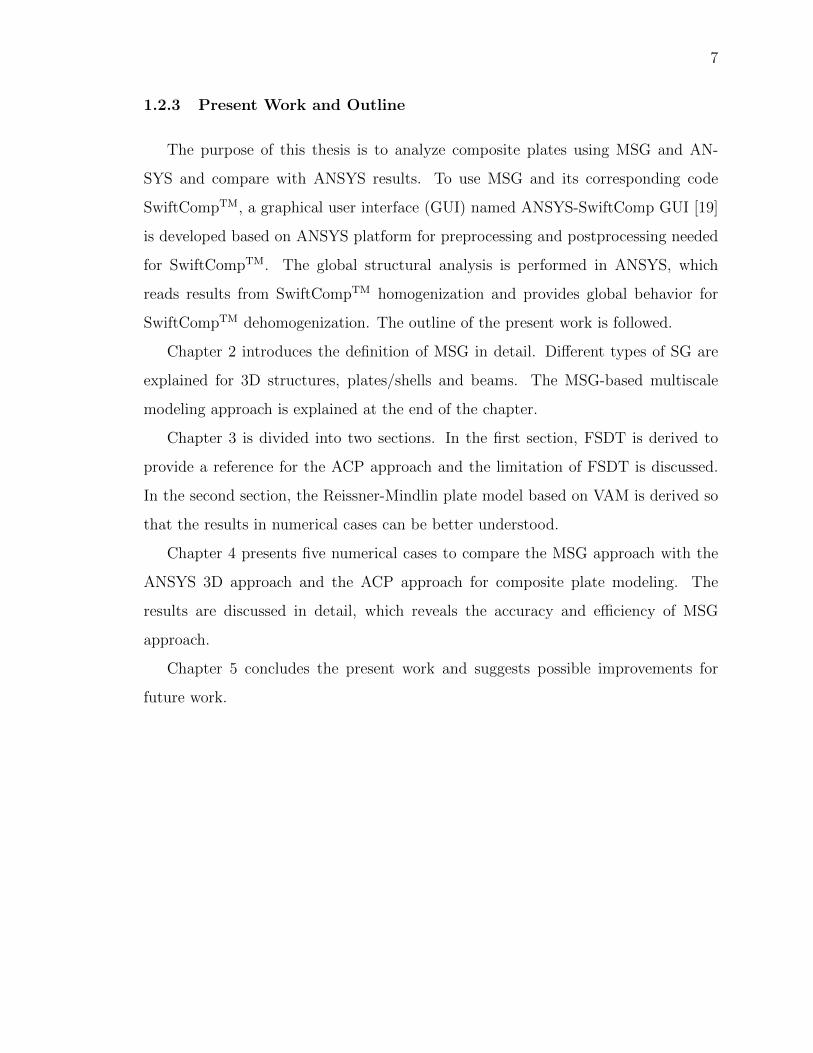
1.2.3 Present Work and Outline
The purpose of this thesis is to analyze composite plates using MSG and AN-
SYS and compare with ANSYS results. To use MSG and its corresponding code
SwiftCompTM, a graphical user interface (GUI) named ANSYS-SwiftComp GUI [19]
is developed based on ANSYS platform for preprocessing and postprocessing needed
for SwiftCompTM. The global structural analysis is performed in ANSYS, which
reads results from SwiftCompTM homogenization and provides global behavior for
SwiftCompTM dehomogenization. The outline of the present work is followed.
Chapter 2 introduces the definition of MSG in detail. Different types of SG are
explained for 3D structures, plates/shells and beams. The MSG-based multiscale
modeling approach is explained at the end of the chapter.
Chapter 3 is divided into two sections. In the first section, FSDT is derived to
provide a reference for the ACP approach and the limitation of FSDT is discussed.
In the second section, the Reissner-Mindlin plate model based on VAM is derived so
that the results in numerical cases can be better understood.
Chapter 4 presents five numerical cases to compare the MSG approach with the
ANSYS 3D approach and the ACP approach for composite plate modeling. The
results are discussed in detail, which reveals the accuracy and efficiency of MSG
approach.
Chapter 5 concludes the present work and suggests possible improvements for
future work.

8
9
2. MECHANICS OF STRUCTURE GENOME
This chapter provides an introduction to Mechanics of Structures Genome (MSG).
MSG is the fundamental framework on which the new approach to analyze composite
plates in this thesis is based. Hence, a brief introduction of MSG is presented in
this chapter to set up the stage for the composite plate modeling using MSG in next
chapter.
2.1 Introduction
In the field of biology, a genome is an organism’s complete set of DNA, which con-
tains all of the information needed to build and maintain that organism. Inspired by
this concept, we can generalize the word genome to represent a fundamental building
block of a system which is not biological. Then a new concept called the Structure
Genome (SG) is defined as the smallest mathematical building block of a structure
by Yu [13]. This definition represents an analogy between two different disciplines:
SG containing all the constitutive information needed for a structure is similar to the
genome containing all the genetic information for an organism’s growth and develop-
ment.
To understand the concept of SG, we need to carefully define the concept of struc-
ture first. Yu [20] clarified the distinction between structures and materials, which
are often used interchangeably in literature. A structure is a solid body made of
one or more materials with clearly defined interactions with its external environment
through boundary conditions, applied loads, and environment effects, (e.g., tempera-
ture and moisture) etc [21]. Despite the complexity of a structure, it can be modeled
using one or more typical components as shown in Figure 2.1. If all three dimensions
of a component are of similar size, it can be called a 3D structure; if one dimension

10
is much smaller than the other two dimensions, it can be called a plate/shell; if two
dimensions are much smaller than the third dimension, it can be called a beam.
Figure 2.1. Typical structure components
Many models have been developed for these structural components. The classical
ones are Cauchy elasticity for 3D structures, Kirchhoff-Love model for plates/shells,
and Euler-Bernoulli model for beams. 3D structures can be considered as 3D models
because the unknown functions are three-variable functions with three coordinates
as independent variables. Plates/shells can be considered as 2D models because
the unknowns functions are two-variable functions with two in-plane coordinates as
independent variables. Beams can be considered as one-dimensional (1D) models
because the unknowns functions are one-variable functions with the axial coordinate
as the independent variable. To this end, beams/plates/shells can be collectively
called dimensionally reducible structures as the models of these structural components
are reduced from the original 3D model [10].
With the definition and categorization of structures in mind, we will then explain
SG for 3D structures, SG for plates/shells and SG for beams in the following sections.
2.2 SG for 3D Structures
For 3D structures, SG is a generalization of the representative volume element
(RVE) concept in micromechanics. As shown in Figure 2.2, depending on the het-
erogeneity of a 3D heterogeneous structure, a SG can be 1D, 2D or 3D. Also a SG
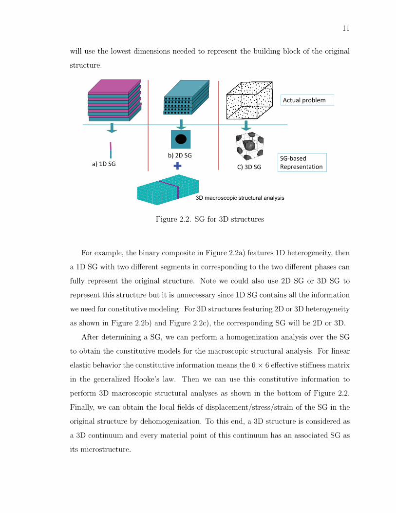
11
will use the lowest dimensions needed to represent the building block of the original
structure.
+
3D macroscopic structural analysis
a) 1D SG
b) 2D SG
C) 3D SG
Actual problem
SG-based
Representa!on
Figure 2.2. SG for 3D structures
For example, the binary composite in Figure 2.2a) features 1D heterogeneity, then
a 1D SG with two different segments in corresponding to the two different phases can
fully represent the original structure. Note we could also use 2D SG or 3D SG to
represent this structure but it is unnecessary since 1D SG contains all the information
we need for constitutive modeling. For 3D structures featuring 2D or 3D heterogeneity
as shown in Figure 2.2b) and Figure 2.2c), the corresponding SG will be 2D or 3D.
After determining a SG, we can perform a homogenization analysis over the SG
to obtain the constitutive models for the macroscopic structural analysis. For linear
elastic behavior the constitutive information means the 6 × 6 effective stiffness matrix
in the generalized Hooke’s law. Then we can use this constitutive information to
perform 3D macroscopic structural analyses as shown in the bottom of Figure 2.2.
Finally, we can obtain the local fields of displacement/stress/strain of the SG in the
original structure by dehomogenization. To this end, a 3D structure is considered as
a 3D continuum and every material point of this continuum has an associated SG as
its microstructure.

12
Thus, a SG has more features than RVE as summarized below:
• A 1D SG can be used to compute the complete set of 3D properties and local
fields for structures with 1D heterogeneity. However, 1D RVE is not common
and can not be used to compute the complete 3D properties and local fields.
• A 2D RVE only obtains in-plane properties and local fields. If the complete
set of properties are needed for 3D structural analysis, a 3D RVE is usually
required [22]. However, there is no such limitation in SG.
• Boundary conditions in terms of displacements and tractions indispensable in
RVE-based models are not needed for SG-based models.
• Because SG-based models does not need to apply displacement or traction
boundary conditions, MSG is more efficient than RVE analysis even for 3D
SGs.
2.3 SG for Plates/Shells
For plate/shell structures, a SG can be 1D, 2D or 3D depending on the hetero-
geneity of the original structure as shown in Figure 2.3. The SGs we use in this
thesis to analyze composite plates belong to this section. If a plate/shell features 1D
heterogeneity as shown in Figure 2.3a), the SG is 1D. For plates/shells featuring 2D
or 3D heterogeneity as shown in Figure 2.3b) and Figure 2.3c), the corresponding SG
will be 2D or 3D.
Same as SG for 3D structures, 1D, 2D or 3D SG for plates/shells will give all con-
stitutive information by homogenization and local fields of displacement/strain/stress
by dehomogenization. And the constitutive information can be used directly for 2D
plate/shell analysis as shown in the bottom of Figure 2.3. Here, however, the con-
stitutive information means plate stiffness matrix, the 6 × 6 stiffness matrix for the
Kirchhoff-Love plate model or the 8 × 8 stiffness matrix for the Reissner-Mindlin
model. To this end, the reference surface of a plate/shell structure is considered as

13
2D plate/shell analysis
+a) 1D SG
b) 2D SGc) 3D SG
Actual problem
SG-based
Representa!on
Figure 2.3. SG for Plates/Shells
a 2D continuum and every material point of this continuum has an associated SG as
its microstructure.
This thesis will use 1D and 2D SGs to model plate/shell structures.
2.4 SG for Beams
For beam structures, a SG can be 2D or 3D depending on the heterogeneity of
the original structure as shown in Figure 2.4. If a beam has uniform cross sections as
shown in 2.4a), the SG is 2D. More specifically, it is a 2D cross-sectional domain. If
the beam is also heterogeneous in the spanwise direction as shown in 2.4b), the SG
will be 3D to represent the fundamental building block of the original beam structure.
Same as SG for 3D structures and plates/shells, 2D or 3D SG for beams will give all
constitutive information by homogenization and local fields of displacement/strain/stress
by dehomogenization. And the constitutive information can be used directly for 1D
beam analysis as shown in the bottom of Figure 2.4. Here, however, the constitu-
tive information means beam stiffness matrix, the 4 × 4 beam stiffness matrix for
Euler-Bernoulli beam model or the 6 × 6 beam stiffness matrix for Timoshenko beam
14
+
1D beam analysis
a) 2D SG
b) 3D SG
Reference line
Reference line
Reference line
Actual problem
SG-based
Representa!on
Figure 2.4. SG for Beams
model. To this end, the beam reference line of a beam structure is considered as a
1D continuum and every material point of this continuum has an associated SG as
its microstructure.
2.5 MSG-based Multiscale Structural Modeling
Now we have clearly defined the meaning of SG. Then for different structures, MSG
provides a rigorous and systematic approach to compute constitutive information
(homogenization) and local fields (dehomogenization) within the original structures.
To use MSG approach practically, MSG-based multiscale structural modeling ap-
proach is introduced. It can be used to fill the gap between material genome and
macroscopic structural analysis and can directly connect with simple structural ele-
ments (3D solid elements, plate/shell elements or beam elements) available in stan-
dard FEA software packages, such as shell elements in ANSYS.
The work flow of MSG is shown in Figure 2.5. First, MSG starts from the original
model. Note the original model here means 3D continuum mechanics. Next, we iden-
tify SG based on the nature of original model and engineering experience. Then, MSG

15
uses the principle of minimum information loss (PMIL) based on the powerful varia-
tional asymptotic method (VAM) to decouple the original problem to a constitutive
modeling over the SG and a structural analysis. The constitutive modeling has been
implemented in a general-purpose software named SwiftCompTM, which is developed
by Professor Wenbin Yu at Purdue University. SwiftCompTM can provide the con-
stitutive models needed for the structural analysis by homogenization and pointwise
local fields of displacement/strain/stress by dehomogenization. The global structural
analysis could be easily handled by standard FEA software package such as ANSYS,
which provides the global behavior for SwiftCompTM to perform dehomogenization.
Figure 2.5. Work flow of Mechanics of Structure Genome

16
17
3. EQUIVALENT SINGLE LAYER PLATE THEORIES
The MSG in the above chapter is very general, which covers three major areas, i.e. 3D
structures, plates/shells and beams. For a realistic scope, this thesis only considers a
subset of MSG, i.e., plate-like structure for simplicity. In this chapter, the FSDT will
be derived first to provide a reference for the ACP approach. The limitations of FSDT
will be discussed in detail. Then the Reissner-Mindlin model based on VAM will be
derived as a theory reference for the MSG approach. With these two derivations, the
numerical cases in the next chapter can be better understood. Please note that all
the derivations only reflect the author’s understanding of the originally publication.
All credits should go to the original authors [9, 10,23,24].
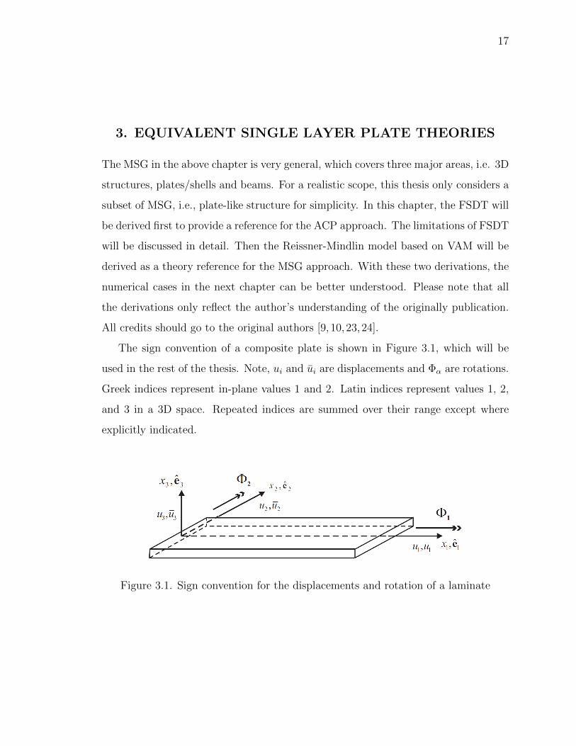
The sign convention of a composite plate is shown in Figure 3.1, which will be
used in the rest of the thesis. Note, ui and ui are displacements and Φα are rotations.
Greek indices represent in-plane values 1 and 2. Latin indices represent values 1, 2,
and 3 in a 3D space. Repeated indices are summed over their range except where
explicitly indicated.
Figure 3.1. Sign convention for the displacements and rotation of a laminate
18
3.1 First Order Shear Deformation Theory
3.1.1 Kinematics
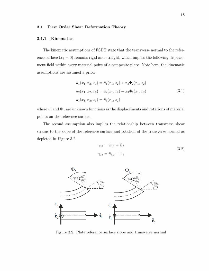
The kinematic assumptions of FSDT state that the transverse normal to the refer-
ence surface (x3 = 0) remains rigid and straight, which implies the following displace-
ment field within every material point of a composite plate. Note here, the kinematic
assumptions are assumed a priori.
u1(x1, x2, x3) = u1(x1, x2) + x3Φ2(x1, x2)
u2(x1, x2, x3) = u2(x1, x2)− x3Φ1(x1, x2)
u3(x1, x2, x3) = u3(x1, x2)
(3.1)
where ui and Φα are unknown functions as the displacements and rotations of material
points on the reference surface.
The second assumption also implies the relationship between transverse shear
strains to the slope of the reference surface and rotation of the transverse normal as
depicted in Figure 3.2.
γ13 = u3,1 + Φ2
γ23 = u3,2 − Φ1
(3.2)
Figure 3.2. Plate reference surface slope and transverse normal
19
The infinitesimal strain defined in the 3D linear elasticity theory is.
εij =1
2(ui,j + uj,i) (3.3)
Substituting the displacement field in Eq. (3.1) into the definition of infinitesimal
strain in Eq. (3.3), we get the 3D strain field within very material point of a composite
plate.
ε11(x1, x2, x3) = u1,1(x1, x2) + x3Φ2,1(x1, x2)
2ε12(x1, x2, x3) = u1,2(x1, x2) + u2,1(x1, x2) + x3[Φ2,2(x1, x2)− Φ1,1(x1, x2)]
ε22(x1, x2, x3) = u2,2(x1, x2)− x3Φ1,2(x1, x2)
2ε13(x1, x2, x3) = u3,1(x1, x2) + Φ2(x1, x2)
2ε23(x1, x2, x3) = u3,2(x1, x2)− Φ1(x1, x2)
ε33(x1, x2, x3) = 0
(3.4)
Introducing 2D plate strain measures for FSDT
εαβ =1
2(uα,β + uβ,α)
κ11 = Φ2,1, κ22 = −Φ1,2, κ12 =1
2[Φ2,2 − Φ1,1]
(3.5)
Substituting 2D plate strain measures in Eqs. (3.5) and (3.2) into Eq. (3.4), we
can express the 3D strain field in terms of 2D unknown plate strain measures as:
εαβ(x1, x2, x3) = εαβ(x1, x2) + x3καβ(x1, x2)
2εα3(x1, x2, x3) = γα3(x1, x2)
ε33(x1, x2, x3) = 0
(3.6)
At this point, the original 3D strain fields are expressed in terms of 2D plate
strains and the thickness coordinate x3.
3.1.2 Constitutive Relations
In FSDT, we assume each layer is made of homogeneous monoclinic material and
the transverse normal stress is equal to zero. The constitutive relation of each layer
in 3D linear elasticity theory is:
20
εe
2εs
εt
=
Se 0 Set
0 Ss 0
STet 0 St
σe
σs
σt
(3.7)
where
εe =
ε11
ε22
2ε12
2εs =
2ε13
2ε23
εt =ε33
σe =
σ11
σ22
σ12
σs =
σ13
σ23
σt =σ33
=
0
Se =
S11 S12 S16
S12 S22 S26
S16 S26 S66
Set =
S13
S23
S36
Ss =
S55 S45
S45 S44
St =[S33
]
Eq. (3.7) implies the relationship between in-plane strains and in-plane stresses
εe = Seσe (3.8)
or the plane-stress reduced stress-strain relations
σe = Qεe (3.9)
where the plane-stress reduced stiffness matrix Q = S−1e depends on the material and
orientation of a layer, which can be expressed explicitly as
Q = RσeQ′RT
σe (3.10)
where Q′ is the plane-stress reduced stiffness matrix in the material coordinate system
and Rσe is the in-plane stress transformation matrix for plane stress state, i.e.,
Q′−1 = S ′e =
1E1
−ν12E1
η12,1G12
−ν12E1
1E2
η12,2G12
η12,1G12
η12,2G12
1G12
Rσe =
c2 s2 −2sc
s2 c2 2sc
sc −sc c2 − s2
(3.11)

21
where E1, E2, ν12, G12, η12,1, η12,2 are engineering constants of this layer in the material
coordinate system. c = cos θ, s = sin θ with θ denoting the layup angle.
The 3D constitutive relations in Eq. (3.7) also imply the relationship between
transverse shear strains and transverse shear stresses as
2εs = Ssσs (3.12)
where Ss is the transverse shear compliance matrix. The inverse relations are
σs = Q∗(2εs) (3.13)
where the transverse shear stiffness matrix Q∗ = S−1s depends on the material and
orientation of a layer, which can be expressed explicitly as
Q∗ = RσsQ∗′RT
σs (3.14)
where Q∗′ is the transverse shear stiffness matrix in the material coordinate system
and Rσs is the transverse stress transformation matrix, i.e.,
Q∗′−1 = S ′s =
1G13
µ23,13G23
µ23,13G23
1G23
Rσs =
c −ss c
(3.15)
where G23, G13, µ13,23, µ23,13 are engineering constants of this layer in the material
coordinate system.
Eqs. (3.7) also implies that the transverse normal strain can be expressed as
ε33 = STetσe (3.16)
Now, in order to express the 3D constitutive relations into its 2D counterpart, we
introduce stress resultant Nαβ,Mαβ and Nα3
Nαβ = 〈σαβ〉
Mαβ = 〈x3σαβ〉N13
N23
= K
〈σ13〉
〈σ23〉
(3.17)
22
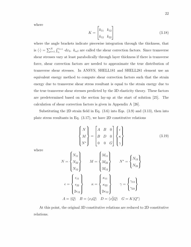
where
K =
k11 k12
k12 k22
(3.18)
where the angle brackets indicate piecewise integration through the thickness, that
is 〈·〉 =∑N
i=1
∫ zi+1
zi·dx3. kαβ are called the shear correction factors. Since transverse
shear stresses vary at least parabolically through layer thickness if there is transverse
force, shear correction factors are needed to approximate the true distribution of
transverse shear stresses. In ANSYS, SHELL181 and SHELL281 element use an
equivalent energy method to compute shear correction factors such that the strain
energy due to transverse shear stress resultant is equal to the strain energy due to
the true transverse shear stresses predicted by the 3D elasticity theory. These factors
are predetermined based on the section lay-up at the start of solution [25]. The
calculation of shear correction factors is given in Appendix A [26].
Substituting the 2D strain field in Eq. (3.6) into Eqs. (3.9) and (3.13), then into
plate stress resultants in Eq. (3.17), we have 2D constitutive relations
N
M
N∗
=
A B 0
B D 0
0 0 G
ε
κ
γ
(3.19)
where
N =
N11
N22
N12
M =
M11
M22
M12
N∗ =
N13
N23
ε =
ε11
ε22
2ε12
κ =
κ11
κ22
2κ12
γ =
γ13
γ23
A = 〈Q〉 B = 〈x3Q〉 D = 〈x2
3Q〉 G = K〈Q∗〉
At this point, the original 3D constitutive relations are reduced to 2D constitutive
relations.
23
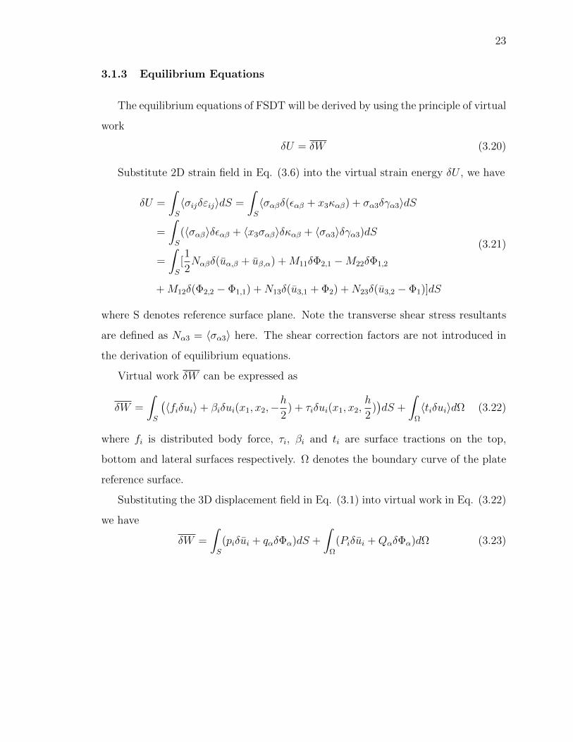
3.1.3 Equilibrium Equations
The equilibrium equations of FSDT will be derived by using the principle of virtual
work
δU = δW (3.20)
Substitute 2D strain field in Eq. (3.6) into the virtual strain energy δU , we have
δU =
∫S
〈σijδεij〉dS =
∫S
〈σαβδ(εαβ + x3καβ) + σα3δγα3〉dS
=
∫S
(〈σαβ〉δεαβ + 〈x3σαβ〉δκαβ + 〈σα3〉δγα3)dS
=
∫S
[1
2Nαβδ(uα,β + uβ,α) +M11δΦ2,1 −M22δΦ1,2
+M12δ(Φ2,2 − Φ1,1) +N13δ(u3,1 + Φ2) +N23δ(u3,2 − Φ1)]dS
(3.21)
where S denotes reference surface plane. Note the transverse shear stress resultants
are defined as Nα3 = 〈σα3〉 here. The shear correction factors are not introduced in
the derivation of equilibrium equations.
Virtual work δW can be expressed as
δW =
∫S
(〈fiδui〉+ βiδui(x1, x2,−
h
2) + τiδui(x1, x2,
h
2))dS +
∫Ω
〈tiδui〉dΩ (3.22)
where fi is distributed body force, τi, βi and ti are surface tractions on the top,
bottom and lateral surfaces respectively. Ω denotes the boundary curve of the plate
reference surface.
Substituting the 3D displacement field in Eq. (3.1) into virtual work in Eq. (3.22)
we have
δW =
∫S
(piδui + qαδΦα)dS +
∫Ω
(Piδui +QαδΦα)dΩ (3.23)

24
Where fi, βi, τi, ti, pi, qα, Pi, Qα are defined by the equations below
pi(x1, x2) = 〈fi〉+ βi + τi
q1(x1, x2) =h
2(β2 − τ2)− 〈x3f2〉
q2(x1, x2) =h
2(τ1 − β1) + 〈x3f1〉
Pi = 〈ti〉
Q1 = −〈x3t2〉
Q2 = 〈x3t1〉
(3.24)
Substituting virtual strain energy δU in Eq. (3.21) and virtual work δW in Eq.
(3.22) into the principle of virtual work in Eq. (3.20), we have
0 =
∫S
[N11δu1,1 +N12δu1,2 +N12δu2,1 +N22δu2,2 +M11δΦ2,1 −M22δΦ1,2
−M12δΦ1,1 +M12δΦ2,2 +N13δu3,1 +N23δu3,2 + (N13 − q2)δΦ2
− (N23 + q1)δΦ1 − p1δu1 − p2δu2 − p3δu3]dS
−∫
Ω
(P1δu1 + P2δu2 + P3δu3 +Q1δΦ1 +Q2δΦ2)dΩ
(3.25)
Integration by parts, we have
0 =
∫S
[− (N11,1 +N12,2 + p1)δu1 − (N12,1 +N22,2 + p2)δu2
− (N13,1 +N23,2 + p3)δu3 + (M12,1 +M22,2 − q1 −N23)δΦ1
− (M11,1 +M12,2 + q2 −N13)δΦ2
]dS
+
∫Ω
[(n1N11 + n2N12 − P1)δu1 + (n1N12 + n2N22 − P2)δu2
+ (n1N13 + n2N23 − P3)δu3 − (n1M12 + n2M22 +Q1)δΦ1
+ (n1M11 + n2M12 −Q2)δΦ2
]dΩ
(3.26)
25
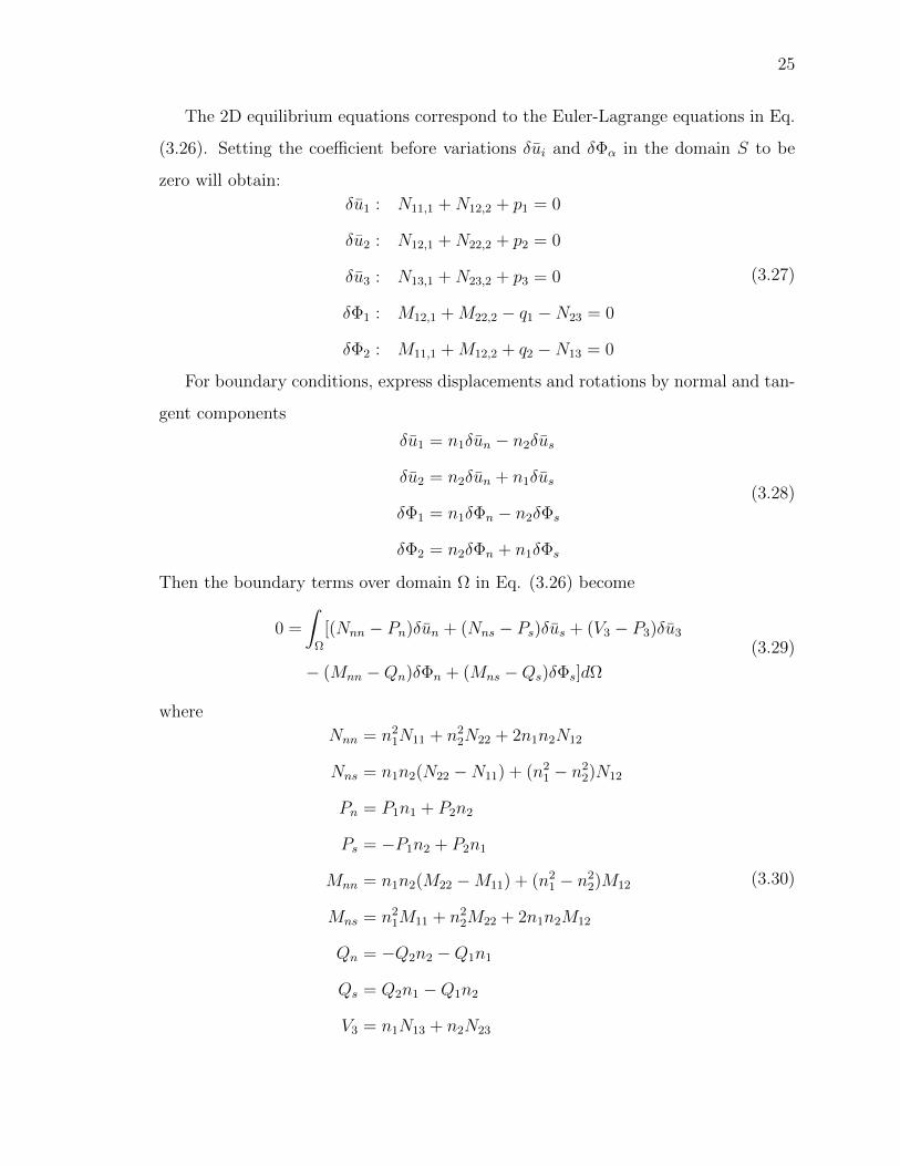
The 2D equilibrium equations correspond to the Euler-Lagrange equations in Eq.
(3.26). Setting the coefficient before variations δui and δΦα in the domain S to be
zero will obtain:
δu1 : N11,1 +N12,2 + p1 = 0
δu2 : N12,1 +N22,2 + p2 = 0
δu3 : N13,1 +N23,2 + p3 = 0
δΦ1 : M12,1 +M22,2 − q1 −N23 = 0
δΦ2 : M11,1 +M12,2 + q2 −N13 = 0
(3.27)
For boundary conditions, express displacements and rotations by normal and tan-
gent components
δu1 = n1δun − n2δus
δu2 = n2δun + n1δus
δΦ1 = n1δΦn − n2δΦs
δΦ2 = n2δΦn + n1δΦs
(3.28)
Then the boundary terms over domain Ω in Eq. (3.26) become
0 =
∫Ω
[(Nnn − Pn)δun + (Nns − Ps)δus + (V3 − P3)δu3
− (Mnn −Qn)δΦn + (Mns −Qs)δΦs]dΩ
(3.29)
where
Nnn = n21N11 + n2
2N22 + 2n1n2N12
Nns = n1n2(N22 −N11) + (n21 − n2
2)N12
Pn = P1n1 + P2n2
Ps = −P1n2 + P2n1
Mnn = n1n2(M22 −M11) + (n21 − n2
2)M12
Mns = n21M11 + n2
2M22 + 2n1n2M12
Qn = −Q2n2 −Q1n1
Qs = Q2n1 −Q1n2
V3 = n1N13 + n2N23
(3.30)

26
Equation (3.29) implies that there are two sets of boundary conditions including
displacement boundary conditions:
un = u0n, us = u0
s, u3 = u03, Φn = Φ0
n, Φs = Φ0s on Ωu (3.31)
and force boundary conditions:
Nnn = Pn, Nns = Ps, Vn3 = P3, Mnn = Qn, Mns = Qs on Ωf (3.32)
Here the portion of the boundary curve where the displacement is prescribed is de-
noted by Ωu, and the portion of the boundary curve where the force is prescribed is
denoted by Ωf . And they have the relationship
Ωu ∩ Ωf = 0
Ωu ∪ Ωf = Ω(3.33)
3.1.4 Limitations
• As a direct result of kinematic assumptions, transverse normal strain ε33 is
zero as shown in Eq. (3.6). This contradicts with the transverse normal stress
assumption σ33 = 0 in Eq. (3.7) which results a nonzero transverse normal
strain in Eq. (3.16) unless the Poison’s ratio is zero. However, FSDT uses the
strain field from kinematic assumptions along with σ33 = 0 in reduced stress-
strain relations to derive 2D constitutive relations and equilibrium equations.
• The transverse stress results are not accurate. If there is transverse shear force,
the transverse shear stress should be at least parabolic along the thickness
whereas it is a constant in FSDT. Besides, the transverse normal stress is always
zero by assumption. This directly ignores that fact that transverse normal stress
exists if there is transverse load.
• The calculation of shear correction factors kαβ is tedious. There are many
different formulas to calculate kαβ in literature. And the calculation of kαβ takes
many factors into consideration such as the material and fiber orientation. The
accuracy of transverse shear stress depends greatly on kαβ.
27
3.2 The Reissner-Mindlin Plate Model Based on VAM
The ad hoc assumptions made by FSDT create many limitations as pointed out
in the above section. However, the Reissner-Mindlin plate model based on VAM has
no ad hoc assumptions as to be derived in the following. For simplicity, the following
derivation only gives dimensional reduction up to the first order.
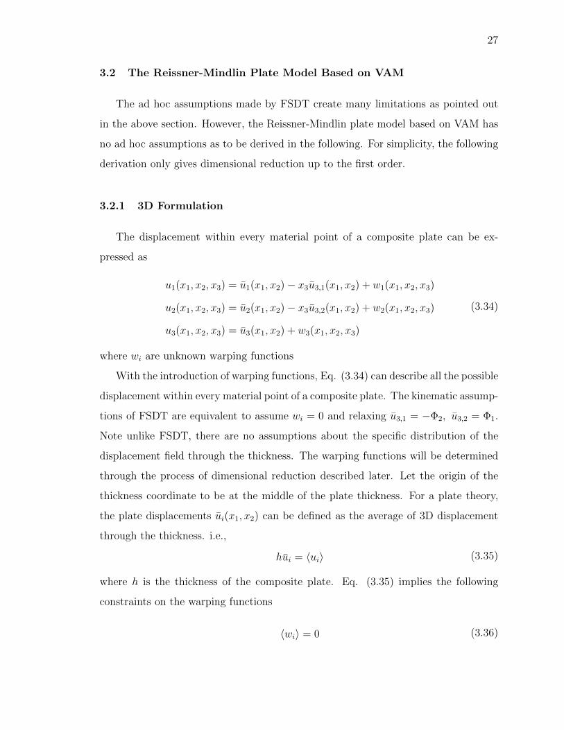
3.2.1 3D Formulation
The displacement within every material point of a composite plate can be ex-
pressed as
u1(x1, x2, x3) = u1(x1, x2)− x3u3,1(x1, x2) + w1(x1, x2, x3)
u2(x1, x2, x3) = u2(x1, x2)− x3u3,2(x1, x2) + w2(x1, x2, x3)
u3(x1, x2, x3) = u3(x1, x2) + w3(x1, x2, x3)
(3.34)
where wi are unknown warping functions
With the introduction of warping functions, Eq. (3.34) can describe all the possible
displacement within every material point of a composite plate. The kinematic assump-
tions of FSDT are equivalent to assume wi = 0 and relaxing u3,1 = −Φ2, u3,2 = Φ1.
Note unlike FSDT, there are no assumptions about the specific distribution of the
displacement field through the thickness. The warping functions will be determined
through the process of dimensional reduction described later. Let the origin of the
thickness coordinate to be at the middle of the plate thickness. For a plate theory,
the plate displacements ui(x1, x2) can be defined as the average of 3D displacement
through the thickness. i.e.,
hui = 〈ui〉 (3.35)
where h is the thickness of the composite plate. Eq. (3.35) implies the following
constraints on the warping functions
〈wi〉 = 0 (3.36)

28
The 3D strain field is obtained by substituting Eq. (3.34) into the definition of
infinitesimal strain in Eq. (3.3)
ε11 = u1,1 − x3u2,11 + w1,1
2ε12 = u1,2 + u2,1 − 2x3u3,12 + w1,2 + w2,1
ε22 = u2,2 − x3u1,22 + w2,2
2ε13 = w1,3 + w3,1
2ε23 = w2,3 + w3,2
ε33 = w3,3
(3.37)
Introducing 2D strain measures as
εαβ =1
2(uα,β + uβ,α)
καβ = −u3,αβ
(3.38)
Note here καβ are different from the curvatures defined in FSDT (3.5). The curvatures
here are the same as what defined in CLPT. They will be transferred to the Mindlin-
Reissner model later.
Substituting Eq. (3.38) into Eq. (3.37). The 3D strain field can be expressed as:
εe = ε+ x3κ+ Iαw‖,α
2εs = w‖′ + eαw3,α
εt = w3′
(3.39)
where
εe =
ε11
ε22
2ε12
2εs =
2ε13
2ε23
εt =ε33
ε =
ε11
ε22
2ε12
κ =
κ11
κ22
2κ12
29
and
I1 =
1 0
0 1
0 0
I2 =
0 0
1 0
0 1
e1 =
1
0
e2 =
0
1
Then, twice of the strain energy stored in a composite plate can be written as
2U =
∫S
⟨εe
2εs
εt
T
Ce Ces Cet
CTes Cs Cst
CTet CT
st Ct
εe
2εs
εt
⟩dS =
∫S
2UdS (3.40)
Note, the material properties are general anisotropic.
For 3D virtual work done by applied loads, it can be written in two terms
δW = δW 2D + δW∗
(3.41)
where
δW 2D =
∫S
(piδui + q1δu3,2 + q2δu3,1)dS +
∫Ω
(Piδui +Q1δu3,2 +Q2δu3,1)dΩ (3.42)
δW∗
=
∫S
(〈fiδwi〉+ τiδw+i + βiδw
−i )dS +
∫Ω
〈tiδwi〉dΩ (3.43)
where ()+ = ()|x3=h2, ()− = ()|x3=−h
2and
pi(x1, x2) = 〈fi〉+ βi + τi
qα(x1, x2) =h
2(βα − τα)− 〈x3fα〉
Pi = 〈ti〉
Qα = −〈x3tα〉
(3.44)
Note the boundary line integral part of δW∗
in Eq. (3.43) represents the work done
through the virtual warping along the lateral boundary of a plate. This term is only
for edge problem, which is beyond the scope of this thesis and will be dropped.
Now, according to the principal of virtual work in Eq. (3.20), we can construct
the problem that has the warping functions as unknown functions to minimize total

30
potential energy density functional and ui are not considered as variable functions.
Note virtual work δW 2D is thus a constant term and will be dropped.
The total potential energy density is
δΠ = 0 with Π = U −W∗ (3.45)
where
δW∗
= δ
∫S
W∗dS (3.46)
with
W∗ = 〈fT‖ w‖〉+ 〈fT
3 w3〉+ τT‖ w
+‖ + τT
3 w+3 + βT
‖ w−‖ + βT
3 w−3 (3.47)
Now, VAM will be used to determine unknown warping functions asymptotically.
3.2.2 Dimensional Reduction
To use VAM, the first step is to assess the order of terms in the potential energy.
Since a composite plate is a plate-like structure, the ratio of thickness to characteristic
length of reference surface is inherently very small, i.e., h/l 1. We will make use of
this small term in dimensional reduction. Since the problem in consideration is a linear
elastic problem, all the strains are assumed to be small. So we have εij ∼ εαβ ∼ ε.
The expressions of strains in Eq. (3.39) imply the order of curvature hκαβ ∼ ε. The
order of strains implies that the order of warping function is either wi ∼ hε or wi ∼ lε.
However, if wi ∼ lε, then ε33 will be in the order of (l/h)ε, which is much larger than
ε. So the order of warping functions can only be hε. Then the orders of derivative of
warping functions are
w‖,α ∼ w3,α ∼h
lε
w‖′ ∼ w3
′ ∼ ε
(3.48)
Consider the 2D plate equilibrium equation in Eqs. (3.27). The orders of surface
traction are
hfα ∼ τα ∼ βα ∼ µh
lε
hf3 ∼ τ3 ∼ β3 ∼ µ(h
l)2ε
(3.49)

31
where µ is the order of material properties.
Zeroth-Order Approximation
Now, the total potential energy density can be written explicitly as
2Π =〈(ε+ x3κ)TCe(ε+ x3κ) + 2(ε+ x3κ)TCeIαw‖,α + 2(Iαw‖,α)TCeIαw‖,α
+ 2(ε+ x3κ)TCesw‖′ + 2(ε+ x3κ)TCeseαw3,α + 2(Iαw‖,α)TCes(w‖
′ + eαw3,α)
+ 2(ε+ x3κ)TCetw3′ + 2(Iαw‖,α)TCetw3
′ + w‖′TCsw‖
′ + 2w‖′TCseαw3,α
+ 2(eαw3,α)TCseαw3,α + 2w‖′TCstw3
′ + 2(eαw3,α)TCstw3′ + Ctw3
′2〉
− 2(〈fT‖ w‖〉+ 〈fT
3 w3〉+ τT‖ w
+‖ + τT
3 w+3 + βT
‖ w−‖ + βT
3 w−3
)(3.50)
where the underlined terms are in the order of h/l or higher and are dropped in the
zeroth-order approximation. The double underlined terms are constants which will
not affect the stationary points and can be simply dropped.
Since the unknown warping functions are subjected to constraints, Lagrange mul-
tiplier method is used. Then the stationary conditions for the total potential energy
density can be obtained from the following variational statement
δI = 0 with I = Π + λ‖〈w‖〉+ λ3〈w3〉 (3.51)
Dropping the underlined and double underlined terms in Eq. (3.50) and leaving
only the leading terms, the variation with respect to the warping functions of the
zeroth-order variational statement is
δI0 =〈[(ε+ x3κ)TCes + w‖′TCs + w3
′CTst]δw‖
′ + λ‖δw‖
+ [(ε+ x3κ)TCet + w‖′TCst + w3
′Ct]δw3′ + λ3δw3〉 = 0
(3.52)
Integration by part, Eq. (3.52) yields the following Euler-Lagrange equations
δw‖ : [(ε+ x3κ)TCes + w‖′TCs + w3
′CTst]′ = λ‖ (3.53)
δw3 : [(ε+ x3κ)TCet + w‖′TCst + w3
′Ct]′ = λ3 (3.54)
32
Since wi are free to vary at top and bottom surfaces, δwi may be not equal to zero.
The boundary conditions from integration by part are
δw‖ : [(ε+ x3κ)TCes + w‖′TCs + w3
′CTst]
+ = 0
[(ε+ x3κ)TCes + w‖′TCs + w3
′CTst]− = 0
(3.55)
δw3 : [(ε+ x3κ)TCet + w‖′TCst + w3
′Ct]+ = 0
[(ε+ x3κ)TCet + w‖′TCst + w3
′Ct]− = 0
(3.56)
Integrating Eq. (3.53) and Eq. (3.54) and substituting boundary conditions from
Eqs. (3.55) and (3.56), we get λ‖ = 0, λ3 = 0 and the Euler-Lagrange equations can
be written as
δw‖ : (ε+ x3κ)TCes + w‖′TCs + w3
′CTst = 0 (3.57)
δw3 : (ε+ x3κ)TCet + w‖′TCst + w3
′Ct = 0 (3.58)
These two equations are satisfied at every point of a composite plate. Solving for
w‖′T and w3
′, we get
w‖′T =− (ε+ x3κ)TC∗esC
−1s
w3′ =− (ε+ x3κ)TC∗etC
∗−1t
(3.59)
where
C∗t =Ct − CTstC−1s Cst
C∗et =Cet − CesC−1s Cst
C∗es =Ces −C∗etC
Tst
C∗t
(3.60)
Substituting the solution of warping functions in Eq. (3.59) back into total potential
energy density in Eq. (3.50) and drop underlined small terms, one can obtain the
total potential energy density asymptotically correct to the zeroth-order as
2Π0 = 〈(ε+ x3κ)TC∗e (ε+ x3κ)〉 =
εκ
T A∗ B∗
B∗T D∗
εκ (3.61)
where
C∗e = Ce − C∗esC−1s CT
es −C∗etC
Tet
C∗t
A∗ = 〈C∗e 〉 B∗ = 〈x3C∗e 〉 D∗ = 〈x2
3C∗e 〉
(3.62)

33
The first approximation coincides with CLPT. However, the transverse strains are not
zero and this procedure does not need ad hoc assumptions regarding the displacement
field or stress field.
The strain field of the zeroth-order approximation can be calculated as
ε0e =ε+ x3κ
2ε0s =w′‖
ε0t =w3
′
(3.63)
The stress field of the zeroth-order approximation can be calculated as
σ0e =C∗e (ε+ x3κ)
2σ0s =0
σ0t =0
(3.64)
First-Order Approximation
In the zeroth-order approximation, the warping functions are in the order of h(hl)0ε
and the total potential energy is in the order of (hl2)µ(hl)0ε2. Perturb the warping
functions to include first-order terms vi, which is in the order of h(hl)ε as expressed
in Eq. (3.65). Continue this process to find first-order approximation. Now the order
of total potential energy is expected to be (hl2)µ(hl)2ε2. We will drop terms greater
than order (h)µ(hl)2ε2 in total potential energy density.
w‖ =w0‖ + v‖
w3 =w03 + v3
(3.65)
Then the orders of derivative of the first-order terms are
v‖,α ∼ v3,α ∼ (h
l)2ε
v‖′ ∼ v3
′ ∼ h
lε
(3.66)
The constraints on warping functions in Eqs. (3.36) lead to the constraints on the
first-order terms

34
〈vi〉 = 0 (3.67)
Since in most engineering problems, a composite layer presents at most monoclinic
material symmetry, we will assume that the layer is monoclinic. So Ces and Cst terms
will vanish in the constitutive relations and the resulting zeroth-order terms become
w0‖ =0
w03 =C⊥E
(3.68)
where
C⊥′ =[−CT
et
Ct−x3
CTet
Ct
](3.69)
and
E =[ε κ
]T
(3.70)
Now, the total potential energy density can be written explicitly as
2Π =〈(ε+ x3κ)TCe(ε+ x3κ) + 2(ε+ x3κ)TCeIαv‖,α + (Iαv‖,α)TCeIαv‖,α
+ 2(ε+ x3κ)TCetw03′+ 2(ε+ x3κ)TCetv3
′ + 2(Iαv‖,α)TCetw03′
+ 2(Iαv‖,α)TCetv3′ + v‖
′TCsv‖′ + 2v‖
′TCseαw03,α + 2v‖
′TCseαv3,α
+ (eαw03,α)TCseαw
03,α + (eαw
03,α)TCseαv3,α + (eαv3,α)TCseαv3,α
+ w03′TCtw
03′+ 2w0
3′TCtv3
′ + v3′TCtv3
′〉 − 2(〈fiw0
i 〉+ τiw0+i + βiw
0−i )
− 2(〈fT‖ v‖〉+ 〈fT
3 v3〉+ τT‖ v
+‖ + τT
3 v+3 + βT
‖ v−‖ + βT
3 v−3
)
(3.71)
Dropping the underlined and double underlined terms in Eq. (3.71) and leaving
only the leading terms, the variation with respect to warping functions of the first-
order variational statement is
δI1 =〈(ε+ x3κ)TC∗e Iαδv‖,α + (v‖′ + eαC⊥E,α)TCsδv‖
′
− fT‖ δv‖ + λ‖δv‖ + v3
′Ctδv3′ + λ3δv3〉
+ τT‖ δv
+‖ + βT
‖ δv−‖ = 0
(3.72)

35
Using integration by parts, Eq. (3.72) yields the following Euler-Lagrange equa-
tions
δv‖ : [Cs(v‖′ + eαC⊥E,α)]′ = Dα
′E,α + g′ + λ‖ (3.73)
δv3 : (v3′TCt)
′ = λ3 (3.74)
where
Dα′ =− IT
α
[C∗e x3C
∗e
]g′ =− f‖
(3.75)
Since vi are free to vary at top and bottom surfaces, δvi may not equal to zero.
The boundary conditions from integration by part are
δv‖ : [Cs(v‖′ + eαC⊥E,α)]+ = τ‖
[Cs(v‖′ + eαC⊥E,α)]− = −β‖
(3.76)
δv3 : (v3′Ct)
+ = 0
(v3′Ct)
− = 0(3.77)
Integrating Eq. (3.74) and substituting boundary conditions in Eq. (3.77), we get
λ3 = 0 and the Euler-Lagrange equation can be written as
δv3 : v3′Ct = 0 (3.78)
This equation is satisfied at every point of a composite plate. Solving for v3′ by
considering the constraints in Eq. (3.67), we get
v3 = 0 (3.79)
In order to solve v‖, integrating Eq. (3.73) with respect to x3
Cs(v‖′ + eαC⊥E,α) = DαE,α + g + λ‖x3 + Λ‖ (3.80)
where Λ‖ is an integration constant.
Substituting boundary conditions in Eq. (3.76), the Lagrange multipliers and
integration constant can be solved to be
λ‖ =1
h(τ‖ + β‖ −D+
α E,α +D−α E,α − g+ + g−)
Λ‖ =1
2(τ‖ − β‖ −D+
α E,α −D−α E,α − g+ − g−)(3.81)

36
Substituting Eqs. (3.81) back into Eq. (3.80) and solving for v‖′, we get
v‖′ = C−1
s D∗αE,α + C−1s g∗ (3.82)
where
D∗α =Dα − CseαC⊥ +x3
hC∓α −
1
2C±α
g∗ =g +x3
hg∓ − 1
2g± + (
x3
h+
1
2)τ‖ + (
x3
h− 1
2)β‖
(3.83)
with the notation ()± = ()+ + ()− and ()∓ = ()− − ()+
Integrating Eq. (3.82) both side, we get the following first-order warping functions
v‖ = DαE,α + g (3.84)
where
Dα′=C−1
s D∗α
〈Dα〉 =0(3.85)
and
g′ =C−1s g∗
〈g〉 =0(3.86)
Substituting the solution of warping functions in Eq. (3.84) back into total po-
tential energy density in Eq. (3.71) and dropping underlined small terms, one can
obtain the total potential energy asymptotically correct to the first-order as
2Π1 = ETAE + ET,1BE,1 + 2ET
,1CE,2 + ET,2DE,2 − 2ETF (3.87)
where
A =
A∗ B∗
B∗T D∗
B =〈Cs(11)C
T⊥C⊥ +D
T
1D1′ +D∗1
Te1C⊥〉
C =〈Cs(12)CT⊥C⊥ +
1
2(D
T
1D2′ +D1
′TD2 +D∗1Te2C⊥ + C⊥
TeT1D∗2)〉
D =〈Cs(22)CT⊥C⊥ +D
T
2D2′ +D∗2
Te2C⊥〉
F =τ3C+⊥
T+ β3C
−⊥
T+ 〈f3C
T⊥〉
+1
2(〈CT
⊥eTαg∗,α +Dα
′Tg,α −DT
αf‖,α〉 −D+T
α τ‖,α −D−T
α β‖,α)
(3.88)
37
and (αβ) in the subscript indicates the α, β th element in the corresponding matrix.
Note the quadratic terms associated with the applied loads are dropped because they
are not functions of 2D generalized strain E .
The strain field of the first-order approximation can be calculated as
ε1e =ε+ x3κ
2ε1s =v‖
′ + eαw03 ,α
ε1t =w0
3′
(3.89)
The stress field of the first-order approximation can be calculated as
σ1e =C∗e (ε+ x3κ)
2σ1s =(D∗α + CseαC⊥)E,α + g∗
σ1t =0
(3.90)
3.2.3 Transformation to the Reissner-Mindlin Model
Now, for practical applications and to use the shell elements available in commer-
cial finite element software such as ANSYS, Eq. (3.87) needs to be transformed to a
model having the same form as the Reissner-Mindlin plate theory.
In order to transform into the Reissner-Mindlin model, the transverse shear strains
are introduced
γ =[2γ13 2γ23
]T
(3.91)
The relationship between the 2D generalized strain of the Reissner-Mindlin model,
R, and those of the classical plate model, E , can be written as [10]
E = R−Dαγ,α (3.92)
where
D1 =
0 0 0 1 0 0
0 0 0 0 1 0
T
D2 =
0 0 0 0 1 0
0 0 0 0 0 1
T
(3.93)
R =[ε∗11 2ε∗12 ε∗22 K∗11 2K∗12 K∗22
]T
(3.94)

38
where the in-plane strains ε∗αβ and curvatures K∗αβ are the 2D strain measures in the
Reissner-Mindlin model.
Substituting Eq. (3.92) back into Eq. (3.87) and neglecting higher-order terms,
the total potential density asymptotically correct to the first-order in terms of Reissner-
Mindlin strains can be expressed as
2Π1 =RTAR− 2RTAD2γ,2 − 2RTAD1γ,1
+RT,1BR,1 + 2RT
,1CR,2 +RT,2DR,2 − 2RTF
(3.95)
The total potential energy of the Reissner-Mindlin plate model has the form of
2ΠR =RTAR+ γTGγ − 2RTFR − 2γTFγ (3.96)
Further derivation is needed to eliminate the terms with partial derivatives of
the 2D generalized strains of the Reissner-Mindlin model. From the equilibrium
equations, we have
M11,1 +M12,2 −N13 +m1 = 0
M12,1 +M22,2 −N23 +m2 = 0(3.97)
where m1 = q2 and m2 = −q1.
In the Reissner-Mindlin model, it hasNM = AR− FRN13
N23
= Gγ − Fγ
(3.98)
Combining Eqs. (3.97) and (3.98) together, we have
Gγ − Fγ = DTαAR,α −DT
αAFR,α +
m1
m2
(3.99)
Then the transverse strain can be solved as
γ = G−1Fγ +G−1DTαAR,α −DT
αAFR,α +G−1
m1
m2
(3.100)
39
Substituting Eq. (3.100) back into Eq. (3.95) and dropping higher-order terms
not related with 2D generalized strains, Eq. (3.95) can be rewritten as
2ΠR = RTAR+ γTGγ − 2RTF + U∗ (3.101)
where
U∗ = RT,1BR,1 + 2RT
,1CR,2 +RT,2DR,2 (3.102)
and
B =B + AD1G−1DT
1 A
C =C + AD1G−1DT
2 A
D =D + AD2G−1DT
2 A
(3.103)
If we can drive U∗ to be zero for any R, then we have found an asymptotically
correct Reissner-Mindlin plate model. This can be achieved by using optimization
process such as the least square technique to solve the overdetermined system for
the constants as done in [9]. By the optimization process, the best transverse shear
stiffness matrix G can be obtained to complete the transformation to the Reissner-
Mindlin plate model. There is no need for shear correction factors and the transverse
shear stress can be accurately calculated. We can continue the dimensional reduction
process to obtain second-order approximate, which is needed for accurately recovering
transverse normal stress.
3.2.4 Advantages
• There are no ad hoc assumptions involved in the derivation, which is mathe-
matically more rigorous. No contradictions are created as appeared in FSDT.
• The transverse stress can be accurately recovered in the second-order approx-
imation. Mathematically, the accuracy of the second-order approximation is
comparable to zigzag plate theories with transverse shear stress expressed as a
second-order polynomials.

40
• Shear correction factors are not needed in the derivation of the VAM-based
Reissner-Mindlin model. The transverse shear stiffness matrix G can be ob-
tained by the transformation to the Reissner-Mindlin plate model.
41
4. NUMERICAL EXAMPLES
In this chapter, five numerical cases are provided to demonstrate the accuracy and
efficiency of the MSG-based plate analysis approach. To assess the accuracy, the
corresponding equivalent 3D finite element models created by ANSYS solid element
(ANSYS 3D approach) are provided as reference. To evaluate the efficiency, the 2D
models created by ANSYS Composite PrepPost (ACP approach) are provided as
comparison.
The modeling framework of the MSG approach is shown in Figure 4.1. The
detailed steps are explained below.
Figure 4.1. Modeling framework of the MSG approach

42
The first three cases will use 1D SG. The forth and fifth cases will use 2D SG.
Having identified the SG, we will use SwiftCompTM to conduct SG homogenization
analysis, whose input file, ∗.sc, is generated by ANSYS-SwiftComp GUI. Then we
get the results of the homogenization analysis, i.e, A, B, D matrix. To get G matrix,
VAPAS will be used instead. Note, in the current version of SwiftCompTM, the
Reissner-Mindlin model has not been included yet. So VAPAS will be used if the
Reissner-Mindlin model is needed. In ANSYS, we can input A, B, D, G matrix
directly into SHELL281 element for the macroscopic structural analysis. Then we
obtain displacements for each node and 2D strain measures, i.e, εαβ, καβ and γα3
for each element. Next, we identify the point we are interested in to recover local
field. Note, we may need several nodes/elements around this point and use the
finite difference method to get the derivative of 2D strain measures at this point
in order to accurately recover the local field if we use VAPAS. Next, we will use
SwiftCompTM again to perform dehomogenization analysis, whose input file, ∗.glb, is
generated by ANSYS-SwiftComp GUI. Finally, we get the local pointwise distribution
of displacements/stresses/strains over the SG.
For the ANSYS 3D approach, SOLID186 element will be used to create the refer-
ence model. Note, the ANSYS version used in all the cases is 17.1.
For the ACP approach, the geometry and layup information will be created in
ANSYS Composite PrePost, which will generate the corresponding APDL files in
ANSYS Workbench.

43
4.1 Case 1: A 6-layer Symmetric Thin Laminate
The first case is a [0/30/-30]s laminate. All the layers have same thickness of
0.01 inch. Each layer is assumed to be orthotropic. The lamina constants of the
composites are E1 = 20 × 106 psi, E2 = E3 = 1.45 × 10⁶ psi, G12 = G13 = 106 psi,
G23 = 4.86577 × 10⁶ psi, ν12 = ν13 = 0.3, ν23 = 0.49. The geometry and boundary
conditions are depicted in Figure 4.2. It is clamped at x1 = −0.5 and subjected to a
uniform pressure P = 100 psi at the top surface along the negative x3 direction. The
ratio of in-plane dimension to thickness is 16.67.
Figure 4.2. Geometry and boundary condition for case 1
The detailed steps for the MSG approach will be presented for case 1 as a demon-
stration. Other cases will follow a similar procedure and detailed steps are not re-
peated for simplicity.
First, the SG for case 1 is 1D. This 1D SG can be easily created in ANSYS-
SwiftComp GUI. Click Preprocessor → Common SG → 1D SGs → Fast Generate.
Then input Material number, Layup and Ply thickness for this laminate, i.e., 1,
′[0/30 − 30]s′ and 0.01 respectively. For detailed instructions of creating a common
SG, an introduction to ANSYS-SwiftComp GUI is given in Appendix B.

44
After creating 1D SG, the next step is to perform homogenization analysis to
get A, B, D and G matrices of the laminate. Click Preprocessor → Solution →
Homogenization → Plate/Shell Model. Keep default parameters and click OK. The
effective properties will automatically pop up. Note, to get G matrix, VAPAS is used.
The input file of SwiftCompTM can be easily modified to be the input files of VAPAS.
The third step is to perform global structural analysis. SHELL281 element is used
to directly read A, B, D and G matrix. The mesh and boundary conditions are the
same with the ACP approach. In order to input global behaviors for dehomogeniza-
tion analysis, output the displacements values of a node at the center (x1 = 0, x2 = 0)
as well as displacement values of 8 nodes neighboring to the center node. The 2D
strain measures of 16 elements neighboring to the center node are also printed.
The last step is dehomogenization analysis. The finite difference method is used
to get the global behaviors at the center node, if the dehomogenization is carried out
by VAPAS, which needs the derivatives of 2D strain measures, i.e.,
εαβ,1, καβ,1, εαβ,2, καβ,2, εαβ,11, καβ,11, εαβ,12, καβ,12, εαβ,22, καβ,22
In order to demonstrate the accuracy and efficiency of using the MSG approach,
all the cases will also be analyzed by the ANSYS 3D approach and the ACP approach.
Note, we will call the ANSYS 3D approach, the ACP approach and the MSG approach
as ANSYS 3D, ACP and MSG respectively in all the cases for simplicity.
For case 1, ANSYS 3D has 614, 400 elements and 2, 558, 129 nodes. There are 4
elements through the thickness of each layer. The reason that using such a fine mesh
with approximately unity aspect ratio is to get the results converged so the model
of ANSYS 3D can be treated as the reference. Both MSG and ACP have 25, 600
elements and 77, 441 nodes for the 2D plate analysis. In addition, MSG uses 6 more
line elements with 25 nodes for MSG homogenization and dehomogenization analysis.
The total number of elements and nodes of the three approaches are summarized in
Table 4.1.
The displacement u3 by the three approaches is shown in Figure 4.3. The dis-
placement values are taken along a path from point (−0.5, 0, 0) to point (0.5, 0, 0).

45
Table 4.1 Finite element mesh information for case 1
Approach Element type Elements Nodes
ANSYS 3D SOLID186 614, 400 2, 558, 129
ACP SHELL281 25, 600 77, 441
MSGSG - 6 25
2D Plate SHELL281 25, 600 77, 441
As we can see, the displacement u3 of both MSG and ACP agree well with ANSYS
3D.
−0.5 −0.4 −0.3 −0.2 −0.1 0 0.1 0.2 0.3 0.4 0.5−0.045
−0.04
−0.035
−0.03
−0.025
−0.02
−0.015
−0.01
−0.005
0
x1 (in)
u3 (
in)
ANSYS 3D
ACP
MSG
Figure 4.3. Comparison of deflection u3 along x1 at x2 = x3 = 0 for case 1
The stresses obtained from the three approaches are also compared. The stress
values are taken through thickness at the center node (x1 = 0, x2 = 0). For ANSYS
3D, it is taken along a path from point (0, 0,−0.03) to point (0, 0, 0.03). For ACP, it
is taken from data at TOP and BOTTOM for all layers. For MSG, the results are
from dehomogenization.

46
For in-plane stresses, both MSG and ACP agree well with ANSYS 3D as shown
from Figure 4.4 to Figure 4.6.
−0.03 −0.02 −0.01 0 0.01 0.02 0.03−2.5
−2
−1.5
−1
−0.5
0
0.5
1
1.5
2
2.5x 10
4
x3 (in)
σ1
1 (
psi)
ANSYS 3D
ACP
MSG
Figure 4.4. Comparison of stress σ11 through thickness for case 1
−0.03 −0.02 −0.01 0 0.01 0.02 0.03−2500
−2000
−1500
−1000
−500
0
500
1000
1500
2000
2500
x3 (in)
σ2
2 (
psi)
ANSYS 3D
ACP
MSG
Figure 4.5. Comparison of stress σ22 through thickness for case 1

47
−0.03 −0.02 −0.01 0 0.01 0.02 0.03−4000
−3000
−2000
−1000
0
1000
2000
3000
4000
x3 (in)
σ1
2 (
psi)
ANSYS 3D
ACP
MSG
Figure 4.6. Comparison of stress σ12 through thickness for case 1
For transverse stresses, the MSG agrees well with ANSYS 3D while ACP loses
accuracy as shown from Figure 4.7 to Figure 4.9.
−0.03 −0.02 −0.01 0 0.01 0.02 0.03−1400
−1200
−1000
−800
−600
−400
−200
0
200
x3 (in)
σ1
3 (
psi)
ANSYS 3D
ACP
MSG
Figure 4.7. Comparison of stress σ13 through thickness for case 1

48
−0.03 −0.02 −0.01 0 0.01 0.02 0.03−180
−160
−140
−120
−100
−80
−60
−40
−20
0
x3 (in)
σ2
3 (
psi)
ANSYS 3D
ACP
MSG
Figure 4.8. Comparison of stress σ23 through thickness for case 1
−0.03 −0.02 −0.01 0 0.01 0.02 0.03−120
−100
−80
−60
−40
−20
0
20
x3 (in)
σ3
3 (
psi)
ANSYS 3D
ACP
MSG
Figure 4.9. Comparison of stress σ33 through thickness for case 1
Specifically, the transverse shear stresses of ACP are piecewise linear while σ13 is
quadratic and σ23 is more complex in ANSYS 3D. It is noted that ACP is a little bit
better than FDST which only predicts a piecewise constant transverse shear stresses.

49
However, MSG is much better than ACP, which has a perfect match with ANSYS
3D. The transverse normal stress of ACP is linear through thickness while σ33 is at
least second order polynomial in ANSYS 3D. Note, ACP is also better than FSDT
since it can recover σ33 independently during the element solution output from the
applied pressure load. Nevertheless, MSG is even better, which perfectly agrees with
ANSYS 3D.
In terms of efficiency, the computation time among the three approaches are com-
pared. It takes 3 hours and 44 seconds to build and solve the model by ANSYS 3D
with 16 CPUs. For MSG, it takes less than 1 minute to build and solve the model
with 2 CPUs. The comparison of computation time for the three approaches is listed
in Table 4.2.
Table 4.2 Computation time for case 1
Approach CPUs Time
ANSYS 3D 16 3 h 44 sec
ACP 2 45 sec
MSG
Homogenization 2 1 sec
34 secStructural analysis 2 32 sec
Dehomogenization 2 1 sec
It is clear that MSG is 2, 551 times more efficient than ANSYS 3D and is even
slightly faster than ACP. The ACP is 11 seconds slower because of the time for
calculation of shear correction factors.

50
4.2 Case 2: A 8-layer Unsymmetrical Thick Laminate
The second case is a [0/90/45/-45/30/-30/75/-75] laminate. All the layers have
same thickness of 0.02 inch. Each layer is assumed to be orthotropic with material
properties being the same as case 1. The geometry and boundary conditions are
depicted in Figure 4.10. It is clamped at x1 = −0.5 and subjected to point force
F3 = −100 lb at (0.5, 0, 0). The ratio of in-plane dimension to thickness is 6.25.
Figure 4.10. Geometry and boundary condition for case 2
The ANSYS 3D has 834, 945 elements and 3, 385, 026 nodes. There are 4 elements
through the thickness of each layer. Both MSG and ACP have 25, 921 elements and
77, 442 nodes for 2D plate analysis. In addition, MSG uses 8 more line elements with
33 nodes for MSG homogenization and dehomogenization analysis. The total number
of elements and nodes of the three approaches are summarized in Table 4.3.
The displacement u3 by the three approaches is shown in Figure 4.11. The dis-
placement values are taken along a path from point (−0.5, 0, 0) to point (0.5, 0, 0).
As we can see, the displacement u3 of both MSG and ACP agree well with ANSYS
3D.

51
Table 4.3 Finite element mesh information for case 2
Approach Element type Elements Nodes
ANSYS 3D SOLID186 834, 945 3, 385, 026
ACP SHELL281 25, 921 77, 442
MSGSG - 8 33
2D Plate SHELL281 25, 921 77, 442
−0.5 −0.4 −0.3 −0.2 −0.1 0 0.1 0.2 0.3 0.4 0.5−0.018
−0.016
−0.014
−0.012
−0.01
−0.008
−0.006
−0.004
−0.002
0
x1 (in)
u3 (
in)
ANSYS 3D
ACP
MSG
Figure 4.11. Comparison of deflection u3 along x1 at x2 = x3 = 0 for case 2
The stresses obtained from the three approaches are compared. The stress values
are taken along thickness at the center node (x1 = 0, x2 = 0). For ANSYS 3D, it is
taken along a path from point (0, 0,−0.08) to point (0, 0, 0.08).
For in-plane stress, both MSG and ACP agree well with ANSYS 3D as shown
from Figure 4.12 to Figure 4.14.
For transverse stresses, the MSG agrees well with ANSYS 3D while ACP loses
accuracy as shown from Figure 4.15 to Figure 4.17. The transverse shear stress σ13
of ACP agrees with ANSYS 3D but slightly worse than MSG. The transverse shear
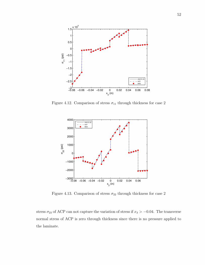
52
−0.08 −0.06 −0.04 −0.02 0 0.02 0.04 0.06 0.08−3
−2.5
−2
−1.5
−1
−0.5
0
0.5
1
1.5x 10
4
x3 (in)
σ1
1 (
psi)
ANSYS 3D
ACP
MSG
Figure 4.12. Comparison of stress σ11 through thickness for case 2
−0.08 −0.06 −0.04 −0.02 0 0.02 0.04 0.06−3000
−2000
−1000
0
1000
2000
3000
4000
x3 (in)
σ2
2 (
psi)
ANSYS 3D
ACP
MSG
Figure 4.13. Comparison of stress σ22 through thickness for case 2
stress σ23 of ACP can not capture the variation of stress if x3 > −0.04. The transverse
normal stress of ACP is zero through thickness since there is no pressure applied to
the laminate.
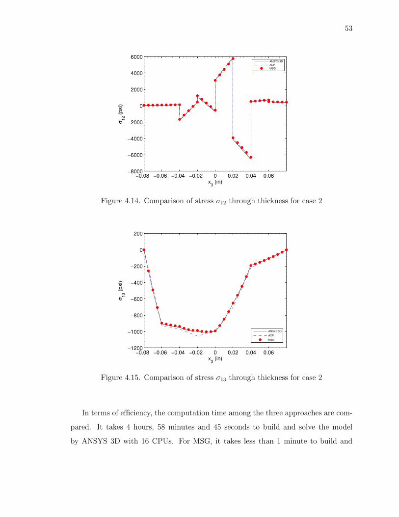
53
−0.08 −0.06 −0.04 −0.02 0 0.02 0.04 0.06−8000
−6000
−4000
−2000
0
2000
4000
6000
x3 (in)
σ1
2 (
psi)
ANSYS 3D
ACP
MSG
Figure 4.14. Comparison of stress σ12 through thickness for case 2
−0.08 −0.06 −0.04 −0.02 0 0.02 0.04 0.06−1200
−1000
−800
−600
−400
−200
0
200
x3 (in)
σ1
3 (
psi)
ANSYS 3D
ACP
MSG
Figure 4.15. Comparison of stress σ13 through thickness for case 2
In terms of efficiency, the computation time among the three approaches are com-
pared. It takes 4 hours, 58 minutes and 45 seconds to build and solve the model
by ANSYS 3D with 16 CPUs. For MSG, it takes less than 1 minute to build and

54
−0.08 −0.06 −0.04 −0.02 0 0.02 0.04 0.06 0.08−50
0
50
100
150
200
x3 (in)
σ2
3 (
psi)
ANSYS 3D
ACP
MSG
Figure 4.16. Comparison of stress σ23 through thickness for case 2
−0.08 −0.06 −0.04 −0.02 0 0.02 0.04 0.06 0.08−7
−6
−5
−4
−3
−2
−1
0
1
x3 (in)
σ3
3 (
psi)
ANSYS 3D
ACP
MSG
Figure 4.17. Comparison of stress σ33 through thickness for case 2
solve the model with 2 CPUs. The comparison of computation time for the three
approaches is listed in Table 4.4.
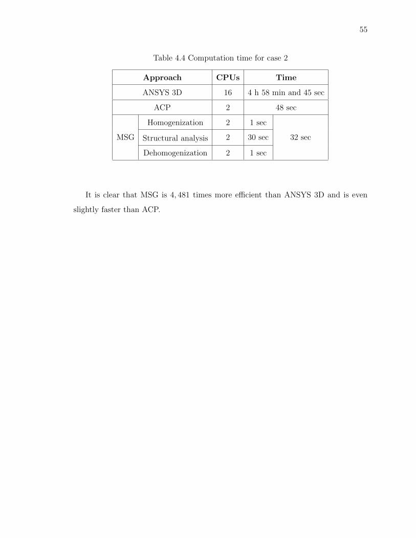
55
Table 4.4 Computation time for case 2
Approach CPUs Time
ANSYS 3D 16 4 h 58 min and 45 sec
ACP 2 48 sec
MSG
Homogenization 2 1 sec
32 secStructural analysis 2 30 sec
Dehomogenization 2 1 sec
It is clear that MSG is 4, 481 times more efficient than ANSYS 3D and is even
slightly faster than ACP.
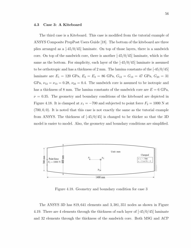
56
4.3 Case 3: A Kiteboard
The third case is a Kiteboard. This case is modified from the tutorial example of
ANSYS Composite PrepPost Users Guide [18]. The bottom of the kiteboard are three
plies arranged as a [-45/0/45] laminate. On top of those layers, there is a sandwich
core. On top of the sandwich core, there is another [-45/0/45] laminate, which is the
same as the bottom. For simplicity, each layer of the [-45/0/45] laminate is assumed
to be orthotropic and has a thickness of 2 mm. The lamina constants of the [-45/0/45]
laminate are E1 = 120 GPa, E2 = E3 = 86 GPa, G12 = G13 = 47 GPa, G23 = 31
GPa, ν12 = ν13 = 0.28, ν23 = 0.4. The sandwich core is assumed to be isotropic and
has a thickness of 8 mm. The lamina constants of the sandwich core are E = 6 GPa,
ν = 0.35. The geometry and boundary conditions of the kiteboard are depicted in
Figure 4.18. It is clamped at x1 = −700 and subjected to point force F2 = 1000 N at
(700, 0, 0). It is noted that this case is not exactly the same as the tutorial example
from ANSYS. The thickness of [-45/0/45] is changed to be thicker so that the 3D
model is easier to model. Also, the geometry and boundary conditions are simplified.
Figure 4.18. Geometry and boundary condition for case 3
The ANSYS 3D has 819, 641 elements and 3, 381, 351 nodes as shown in Figure
4.19. There are 4 elements through the thickness of each layer of [-45/0/45] laminate
and 32 elements through the thickness of the sandwich core. Both MSG and ACP
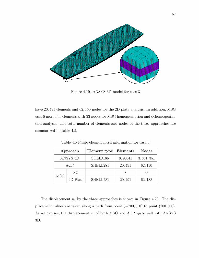
57
Figure 4.19. ANSYS 3D model for case 3
have 20, 491 elements and 62, 150 nodes for the 2D plate analysis. In addition, MSG
uses 8 more line elements with 33 nodes for MSG homogenization and dehomogeniza-
tion analysis. The total number of elements and nodes of the three approaches are
summarized in Table 4.5.
Table 4.5 Finite element mesh information for case 3
Approach Element type Elements Nodes
ANSYS 3D SOLID186 819, 641 3, 381, 351
ACP SHELL281 20, 491 62, 150
MSGSG - 8 33
2D Plate SHELL281 20, 491 62, 188
The displacement u3 by the three approaches is shown in Figure 4.20. The dis-
placement values are taken along a path from point (−700, 0, 0) to point (700, 0, 0).
As we can see, the displacement u3 of both MSG and ACP agree well with ANSYS
3D.

58
−600 −400 −200 0 200 400 6000
0.02
0.04
0.06
0.08
0.1
0.12
0.14
0.16
0.18
0.2
x1 (mm)
u2 (
mm
)
ANSYS 3D
ACP
MSG
Figure 4.20. Comparison of deflection u2 along x1 at x2 = x3 = 0 for case 3
The stresses obtained from the three approaches are compared. The stress values
are taken through thickness at the center node (x1 = 0, x2 = 0). For ANSYS 3D, it
is taken along a path from point (0, 0,−10) to point (0, 0, 10).
−10 −5 0 5 10−0.08
−0.06
−0.04
−0.02
0
0.02
0.04
0.06
0.08
x3 (mm)
σ1
1 (
MP
a)
ANSYS 3D
ACP
MSG
Figure 4.21. Comparison of stress σ11 through thickness for case 3

59
For in-plane stresses, both MSG and ACP agree well with ANSYS 3D as shown
from Figure 4.21 to Figure 4.23.
−10 −5 0 5 10−0.08
−0.06
−0.04
−0.02
0
0.02
0.04
0.06
0.08
x3 (mm)
σ2
2 (
MP
a)
ANSYS 3D
ACP
MSG
Figure 4.22. Comparison of stress σ22 through thickness for case 3
−10 −5 0 5 100
0.05
0.1
0.15
0.2
0.25
0.3
0.35
x3 (mm)
σ1
2 (
MP
a)
ANSYS 3D
ACP
MSG
Figure 4.23. Comparison of stress σ12 through thickness for case 3
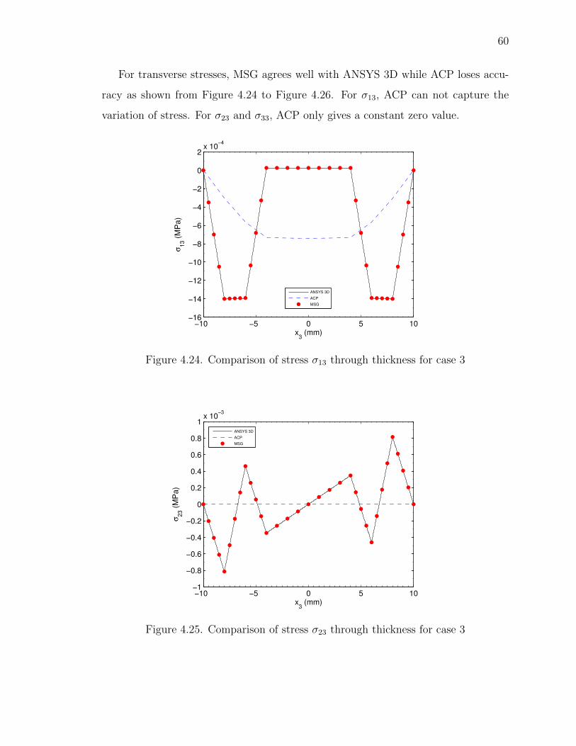
60
For transverse stresses, MSG agrees well with ANSYS 3D while ACP loses accu-
racy as shown from Figure 4.24 to Figure 4.26. For σ13, ACP can not capture the
variation of stress. For σ23 and σ33, ACP only gives a constant zero value.
−10 −5 0 5 10−16
−14
−12
−10
−8
−6
−4
−2
0
2x 10
−4
x3 (mm)
σ1
3 (
MP
a)
ANSYS 3D
ACP
MSG
Figure 4.24. Comparison of stress σ13 through thickness for case 3
−10 −5 0 5 10−1
−0.8
−0.6
−0.4
−0.2
0
0.2
0.4
0.6
0.8
1x 10
−3
x3 (mm)
σ2
3 (
MP
a)
ANSYS 3D
ACP
MSG
Figure 4.25. Comparison of stress σ23 through thickness for case 3
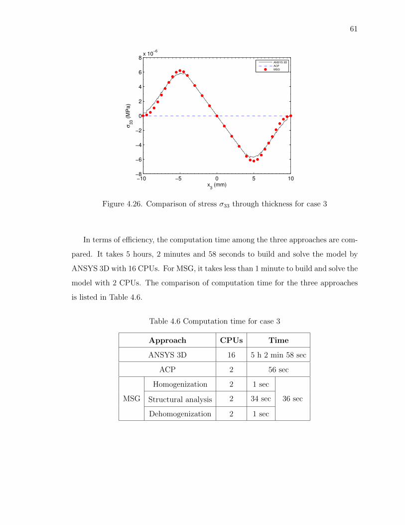
61
−10 −5 0 5 10−8
−6
−4
−2
0
2
4
6
8x 10
−6
x3 (mm)
σ3
3 (
MP
a)
ANSYS 3D
ACP
MSG
Figure 4.26. Comparison of stress σ33 through thickness for case 3
In terms of efficiency, the computation time among the three approaches are com-
pared. It takes 5 hours, 2 minutes and 58 seconds to build and solve the model by
ANSYS 3D with 16 CPUs. For MSG, it takes less than 1 minute to build and solve the
model with 2 CPUs. The comparison of computation time for the three approaches
is listed in Table 4.6.
Table 4.6 Computation time for case 3
Approach CPUs Time
ANSYS 3D 16 5 h 2 min 58 sec
ACP 2 56 sec
MSG
Homogenization 2 1 sec
36 secStructural analysis 2 34 sec
Dehomogenization 2 1 sec

62
It is clear that MSG is 4, 039 times more efficient than ANSYS 3D and is even
slightly faster than ACP.
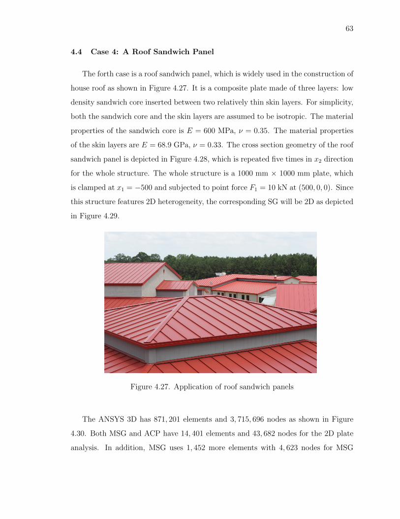
63
4.4 Case 4: A Roof Sandwich Panel
The forth case is a roof sandwich panel, which is widely used in the construction of
house roof as shown in Figure 4.27. It is a composite plate made of three layers: low
density sandwich core inserted between two relatively thin skin layers. For simplicity,
both the sandwich core and the skin layers are assumed to be isotropic. The material
properties of the sandwich core is E = 600 MPa, ν = 0.35. The material properties
of the skin layers are E = 68.9 GPa, ν = 0.33. The cross section geometry of the roof
sandwich panel is depicted in Figure 4.28, which is repeated five times in x2 direction
for the whole structure. The whole structure is a 1000 mm × 1000 mm plate, which
is clamped at x1 = −500 and subjected to point force F1 = 10 kN at (500, 0, 0). Since
this structure features 2D heterogeneity, the corresponding SG will be 2D as depicted
in Figure 4.29.
Figure 4.27. Application of roof sandwich panels
The ANSYS 3D has 871, 201 elements and 3, 715, 696 nodes as shown in Figure
4.30. Both MSG and ACP have 14, 401 elements and 43, 682 nodes for the 2D plate
analysis. In addition, MSG uses 1, 452 more elements with 4, 623 nodes for MSG
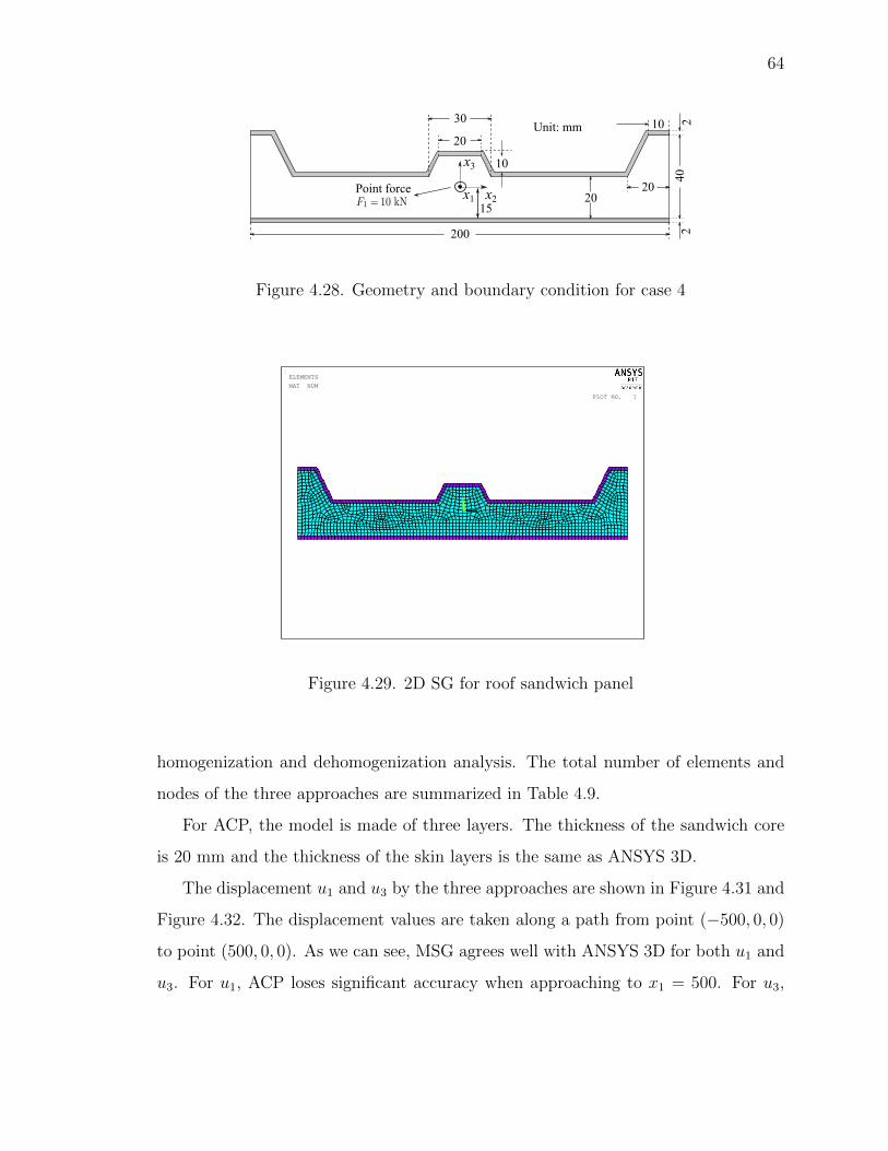
64
Figure 4.28. Geometry and boundary condition for case 4
1
X
Y
Z
PLOT NO. 1
ELEMENTS
MAT NUM
Figure 4.29. 2D SG for roof sandwich panel
homogenization and dehomogenization analysis. The total number of elements and
nodes of the three approaches are summarized in Table 4.9.
For ACP, the model is made of three layers. The thickness of the sandwich core
is 20 mm and the thickness of the skin layers is the same as ANSYS 3D.
The displacement u1 and u3 by the three approaches are shown in Figure 4.31 and
Figure 4.32. The displacement values are taken along a path from point (−500, 0, 0)
to point (500, 0, 0). As we can see, MSG agrees well with ANSYS 3D for both u1 and
u3. For u1, ACP loses significant accuracy when approaching to x1 = 500. For u3,

65
Figure 4.30. ANSYS 3D model case 4
Table 4.7 Finite element mesh information for case 4
Approach Element type Elements Nodes
ANSYS 3D SOLID186 871, 201 3, 751, 696
ACP SHELL281 14, 401 43, 682
MSGSG - 1, 452 4, 623
2D Plate SHELL281 14, 401 43, 682
ACP only gives a constant zero value. Because the point force is applied at the middle
of the thickness, there is no coupling between force and moment in ACP. However,
the coupling exists in 3D model due to the variation of thickness.
The stresses obtained from the three approaches are compared. The stress values
are taken at x1 = 0, x2 = 0 through thickness. Since the shear stress components σ12,
σ13 and σ23 are in the magnitude of 0.1 Pa or less, these stress components are not
compared. For ANSYS 3D, it is taken along a path from point (0, 0,−10) to point
(0, 0, 10).
For σ11, σ22 and σ33, MSG agrees well with ANSYS 3D as shown in 4.33 to Figure
4.35 while ACP loses accuracy. For σ11 and σ22, the loss of accuracy is obvious at the

66
−500 −400 −300 −200 −100 0 100 200 300 400 5000
0.005
0.01
0.015
0.02
0.025
0.03
0.035
x1 (mm)
u1 (
mm
)
ANSYS 3D
ACP
MSG
Figure 4.31. Comparison of deflection u2 along x2 = 0 for case 4
−500 −400 −300 −200 −100 0 100 200 300 400 500−0.14
−0.12
−0.1
−0.08
−0.06
−0.04
−0.02
0
0.02
x1 (mm)
u3 (
mm
)
ANSYS 3D
ACP
MSG
Figure 4.32. Comparison of deflection u2 along x2 = 0 for case 4
skin layers. For σ33, ACP only gives a constant zero value since there is no applied
pressure.

67
−15 −10 −5 0 5 10 150
0.5
1
1.5
2
2.5
3
x3 (mm)
σ1
1 (
MP
a)
ANSYS 3D
ACP
MSG
Figure 4.33. Comparison of stress σ11 through thickness for case 4
−15 −10 −5 0 5 10 15−0.02
0
0.02
0.04
0.06
0.08
0.1
0.12
x3 (mm)
σ2
2 (
MP
a)
ANSYS 3D
ACP
MSG
Figure 4.34. Comparison of stress σ22 through thickness for case 4
In terms of efficiency, the computation time among the three approaches are com-
pared. It takes 6 hours, 21 minutes and 45 seconds to build and solve the model
by ANSYS 3D with 16 CPUs. For MSG, it takes less than 1 minute to build and

68
−15 −10 −5 0 5 10 15−3
−2.5
−2
−1.5
−1
−0.5
0
0.5x 10
−3
x3 (mm)
σ3
3 (
MP
a)
ANSYS 3D
ACP
MSG
Figure 4.35. Comparison of stress σ33 through thickness for case 4
solve the model with 2 CPUs. The comparison of computation time for the three
approaches is listed in Table 4.8.
Table 4.8 Computation time for case 4
Approach CPUs Time
ANSYS 3D 16 6 h 21 min 45 sec
ACP 2 28 sec
MSG
Homogenization 2 5 sec
44 secStructural analysis 2 23 sec
Dehomogenization 2 16 sec
It is clear that MSG is 4, 164 times more efficient than ANSYS 3D.

69
4.5 Case 5: A Corrugated-core Sandwich Panel
The fifth case is a corrugated-core sandwich panel, which is also widely used in
industry because of its high bending stiffness to weight ratio. A sample aluminum
corrugated sandwich panel is illustrated in Figure 4.36. The thin skin layers are high
in stiffness when compared to the corrugated core. For simplicity, both the corrugated
core and skin layers are assumed to be isotropic. The material properties [27] of the
corrugated core is E = 4.5 GPa, ν = 0.225. The material properties of the skin
layers are E = 68.9 GPa, ν = 0.33. The cross section geometry of the corrugated-
core sandwich panel is depicted in Figure 4.37, which is repeated seven times in x2
direction for the whole structure. The whole structure is a 200 mm × 203.7 mm plate,
which is clamped at x1 = −100 and subjected to point force F1 = 10 kN and F2 = 10
kN at (100, 0, 0). Since this structure features 2D heterogeneity, the corresponding
SG will be 2D as depicted in Figure 4.38.
Figure 4.36. Aluminum Corrugated Sandwich Panel
The ANSYS 3D has 1, 422, 401 elements and 6, 958, 887 nodes as shown in Figure
4.39. Both MSG and ACP have 25, 601 elements and 77, 442 nodes for the 2D plate
analysis. In addition, MSG uses 1, 016 more elements with 3, 658 nodes for MSG

70
Figure 4.37. Geometry and boundary condition for case 5
1
X Y
Z
PLOT NO. 1
ELEMENTS
DSYS=100
MAT NUM
Figure 4.38. 2D SG for corrugated-core sandwich panel
homogenization and dehomogenization analysis. The elements number and nodes
number of the three approaches are summarized in Table 4.9.
For ACP, the model is made of three layers. The material properties of the
corrugated core is the smeared material properties of the original core since there are
void. The Poisson’s ratio remains the same while the Young’s modulus of the smeared
corrugated core becomes
E∗ = EAcA
= 4.5× 103 × 44.46
291= 687.53 MPa (4.1)

71
Figure 4.39. The magnitude of displacement by ANSYS 3D for case 5
Table 4.9 Finite element mesh information for case 5
Approach Element type Elements Nodes
ANSYS 3D SOLID186 1, 442, 401 6, 958, 887
ACP SHELL281 25, 601 77, 442
MSGSG - 1, 016 3, 658
2D Plate SHELL281 25, 601 77, 442
where Ac is the area of sandwich the core and A is the area between the the skin
layers (not include the skins) in Figure 4.37.
The displacement u1 and u2 are compared at point (0, 4, 0) as shown in Table
4.10. For u1, both ACP and MSG have difference less than 1% to ANSYS 3D. For
u2, MSG has difference less than 1% to ANSYS 3D while ACP has difference 1.176%
to ANSYS 3D.
The stresses obtained from the three approaches are compared. The stress values
are taken through the thickness along (0, 0, 4) to (0, 0, 6). Since the transverse stress
components σ13, σ23 and σ33 are in the magnitude of 0.1 Pa or less, these stress
components are not compared.

72
Table 4.10 Comparison of u1 and u2 at point (0, 4, 0) for case 5
Approach u1 (mm) u2 (mm)
ANSYS 3D 3.281364E-02 1.798312E-01
ACP 3.290286E-02 1.777169E-01
MSG 3.292460E-02 1.800830E-01
For σ11, σ22 and σ12, MSG agrees well with ANSYS 3D as shown in Figure 4.40
to Figure 4.42 while ACP loses accuracy. The loss of accuracy is obvious at the
corrugated core for σ11 and σ12. And the loss of accuracy is obvious at the skin layer
for σ22.
4 4.5 5 5.5 60
5
10
15
20
25
x3 (mm)
σ1
1 (
MP
a)
ANSYS 3D
ACP
MSG
Figure 4.40. Comparison of stress σ11 through thickness for case 5
In terms of efficiency, the computation time among the three approaches are com-
pared. It takes 5 hours, 20 minutes and 30 seconds to build and solve the model
by ANSYS 3D with 16 CPUs. For MSG, it takes less than 1 minute to build and
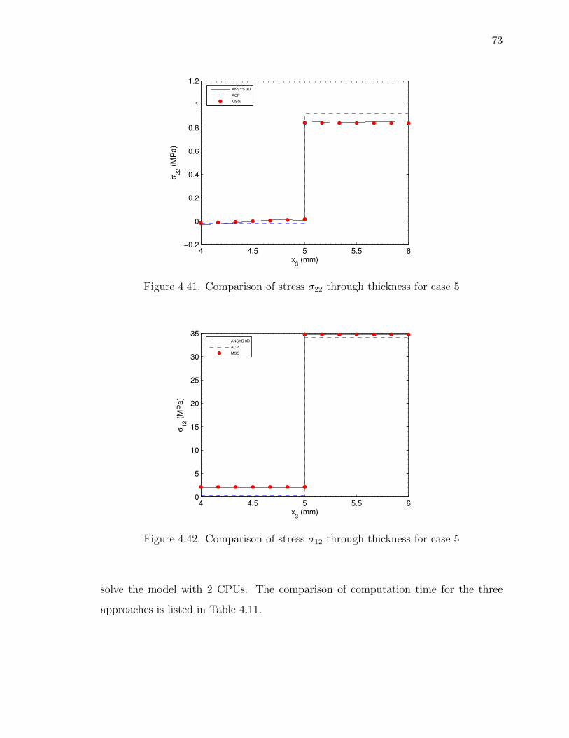
73
4 4.5 5 5.5 6−0.2
0
0.2
0.4
0.6
0.8
1
1.2
x3 (mm)
σ2
2 (
MP
a)
ANSYS 3D
ACP
MSG
Figure 4.41. Comparison of stress σ22 through thickness for case 5
4 4.5 5 5.5 60
5
10
15
20
25
30
35
x3 (mm)
σ1
2 (
MP
a)
ANSYS 3D
ACP
MSG
Figure 4.42. Comparison of stress σ12 through thickness for case 5
solve the model with 2 CPUs. The comparison of computation time for the three
approaches is listed in Table 4.11.
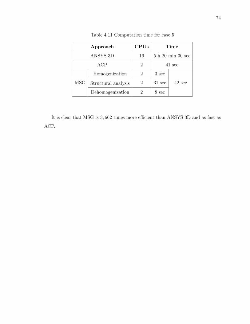
74
Table 4.11 Computation time for case 5
Approach CPUs Time
ANSYS 3D 16 5 h 20 min 30 sec
ACP 2 41 sec
MSG
Homogenization 2 3 sec
42 secStructural analysis 2 31 sec
Dehomogenization 2 8 sec
It is clear that MSG is 3, 662 times more efficient than ANSYS 3D and as fast as
ACP.

75
5. SUMMARY
In this thesis, Mechanics of Structure Genome (MSG) has been used to analyze com-
posite plates. A simple graphic user interface (GUI) named ANSYS-SwiftComp GUI
has been developed based on ANSYS platform as a user friendly GUI to improve the
user friendliness of MSG. The numerical cases show that the MSG approach is not
only accurate but also efficient in comparison to the ANSYS 3D approach and the
ACP approach. The following accomplishments are achieved during this study:
1. ANSYS-SwiftComp GUI has been developed, which can use the preprocessing
and postprocessing capability of ANSYS as a user friendly GUI for SwiftCompTM.
ANSYS-SwiftComp GUI can easily create 1D, 2D or 3D SGs and generate the
corresponding input files for SwiftCompTM homogenization and dehomogeniza-
tion, which greatly enhances the convenience to use SwiftCompTM.
2. The steps of modeling composite plates by using the MSG approach are demon-
strated by five numerical cases. When compared with the ANSYS 3D approach,
the MSG approach agrees well with the results, which reveals its accuracy.
When compared with the ACP approach, the MSG approach presents the same
computational efficiency while being more accurate.
3. The first-order shear deformation theory (FSDT) is derived and compared in
detail with the Reissner-Mindlin plate model based on VAM. The limitations
of FSDT are discussed while the advantages of plate model using VAM are
presented.
Although the power of MSG to analyze composite plates has been shown and the
GUI based on ANSYS has been developed, there are still some work to be continued
and investigated in the future.

76
1. ANSYS SHELL281 or SHELL181 elements can read A, B, D and G matrix and
output global behavior element-wise. However, new shell element is needed to
read the coupling terms Y matrix if one uses Reissner-Mindlin plate model in
SwiftCompTM. Also the new shell element should output global behavior point-
wise at each Gaussian point, which will be more accurate. And the derivatives
of 2D strain measures should also be represented at each Gaussian point if one
uses the Reissner-Mindlin plate model.
2. Present work only used 1D and 2D SGs for composite plates. In some cases such
as honeycomb sandwich structure, only 3D SG can capture the heterogeneity
of the original structure. So some numerical cases by using 3D SGs are needed
to further reveal the capability of MSG.

LIST OF REFERENCES

77
LIST OF REFERENCES
[1] ANSYS Mechanical APDL Element Reference, January 2016. Release 17.0.
[2] R. D. Mindlin. Influence of rotary inertia and shear on flexural motions ofisotropic elastic plates. ASME Journal of Applied Mechanics, 18:31–38, 1951.
[3] E. Reissner. The effect of transverse shear deformation on the bending of elasticplates. ASME Journal of Applied Mechanics, 12:A68–A77, 1945.
[4] R. Khandan, S. Noroozi, P. Sewell, and J. Vinney. The development of laminatedcomposite plate theories: a review. Journal of Materials Science, 47(16):5901–5910, 2012.
[5] J. N. Reddy. A simple higher-order theory for laminated composite plates. Jour-nal of Applied Mechanics, 51(4):745–752, 1984.
[6] V. L. Berdichevskii. Variational-asymptotic method of constructing a theory ofshells: PMM vol. 43, no.4, 1979, pp. 664687. Journal of Applied Mathematicsand Mechanics, 43:711–736, 1979.
[7] A. R. Atilgan and D. H. Hodges. On the strain energy of laminated compositeplates. International Journal of Solids and Structures, 29(20):2527–2543, 1992.
[8] V. G. Sutyrin and D. H. Hodges. On asymptotically correct linear laminatedplate theory. International Journal of Solids and Structures, 33(25):3649–3671,1996.
[9] W. Yu, D. H. Hodges, and V. V. Volovoi. Asymptotic construction of reissner-like composite plate theory with accurate strain recovery. International Journalof Solids and Structures, 39(20):5185–5203, 2002.
[10] W. Yu. Variational asymptotic modeling of composite dimensionally reduciblestructures. PhD thesis, Georgia Institute of Technology, 2002.
[11] W. Yu, D. H. Hodges, and V. V. Volovoi. Asymptotic generalization of reissner–mindlin theory: accurate three-dimensional recovery for composite shells. Com-puter Methods in Applied Mechanics and Engineering, 191(44):5087–5109, 2002.
[12] W. Yu, D. H. Hodges, and V. V. Volovoi. Asymptotically accurate 3-d recov-ery from reissner-like composite plate finite elements. Computers & Structures,81(7):439–454, 2003.
[13] W. Yu. A unified theory for constitutive modeling of composites. Journal ofMechanics of Materials and Structures, 11(4):379–411, 2016.
[14] C. E. S. Cesnik and D. H. Hodges. Vabs: a new concept for composite rotor bladecross-sectional modeling. Journal of the American Helicopter Society, 42(1):27–38, 1997.
78
[15] W. Yu and T. Tang. Variational asymptotic method for unit cell homogeniza-tion of periodically heterogeneous materials. International Journal of Solids andStructures, 44(11):3738–3755, 2007.
[16] X. Liu and W. Yu. A novel approach to analyze beam-like composite struc-tures using mechanics of structure genome. Advances in Engineering Software,100:238–251, 2016.
[17] B. Peng, J. Goodsell, R. B. Pipes, and W. Yu. Generalized free-edge stressanalysis using mechanics of structure genome. Journal of Applied Mechanics,83(10):101013, 2016.
[18] ANSYS Composite PrepPost User’s Guide, January 2016. Release 17.0.
[19] B. Zhao, F. Jiang, Z. Ye, and W. Yu. ANSYS-SwiftComp GUI 1.0 User’s Manual.West Lafayette, IN 47907, May 2016.
[20] W. Yu. Journal Club Theme of October 2015: Mechanics of Structure Genome.http://imechanica.org/node/18928.
[21] W. Yu. SwiftComp User Manual. West Lafayette, IN 47907, July 2016.
[22] C. T. Sun and R. S. Vaidya. Prediction of composite properties from a repre-sentative volume element. Composites Science and Technology, 56(2):171–179,1996.
[23] W. Yu. Classical Plate Model. http://imechanica.org/files/plate.pdf, April 2012.
[24] Y. Long. Asymptotic modelling of a thermopiezoelastic anisotropic smart plate.Master’s thesis, Purdue University, 2015.
[25] ANSYS Mechanical APDL Theory Reference, August 2016. Release 17.2.
[26] ABAQUS Theory Manual Version 6.8, 2008.
[27] I. Dayyani, S. Ziaei-Rad, and M. I. Friswell. The mechanical behavior of com-posite corrugated core coated with elastomer for morphing skins. Journal ofComposite Materials, 48(13):1623–1636, 2014.
[28] F. Jiang and W. Yu. ANSYS-VABS Graphic User Interface (GUI) Release Alpha-1.0 (in updating). West Lafayette, IN 47907, Aug 2015.

APPENDICES

79
A. CALCULATION OF SHEAR CORRECTION FACTORS
Consider a composite plate as shown in Figure 3.1. Assume only bending and shear
in the x1 direction, without gradients in the x2 direction. Then the in-plane forces
in the composite plate are zero N11 = N22 = N12 = 0 and ∂∂x2
= 0 for all response
variables. Then the equilibrium equation in the x1 direction is
σ11,1 + σ13,3 = 0 (A.1)
The 2D equilibrium equations from Eq. (3.27) become
M11,1 −N13 = 0 (A.2)
From Eq. (3.19), we have εκ = H
NM (A.3)
where
H =
A B
B D
−1
We also assume M22 = M12 = 0. Thus,εκ =
[H14 H24 H34 H44 H54 H64
]T
M11 (A.4)
where Hi4 is the fourth column of H. Substituting Eq. (A.4) into Eq. (3.6) and then
into Eq. (3.8), we get in-plane stress components in terms of M11 as
σ11 = (P1 + x3P2)M11 (A.5)
where
P1 = Q11H14 +Q12H24 +Q16H34

80
and
P2 = Q11H44 +Q12H54 +Q16H64
Combining the gradient of this equation with the equilibrium equations in Eq.
(A.1) and Eq. (A.2), we get
σ13,3 = −(P1 + x3P2)N13 (A.6)
A composite plate consists of N layers 1, 2, 3, ... with different values of (P 11 , P
12 )
at layer 1, (P 21 , P
22 ) at layer 2, ... (PN
1 , PN2 ) at layer N . Layer i extends from zi to
zi+1 and its thickness is ti = zi+1 − zi. Integrating Eq. (A.6) through the plate and
using the boundary conditions σ13 = 0 at x3 = 0, σi13 = σi+113 at x3 = zi+1 and σ13 = 0
at x3 = zN+1, gives the transverse shear stress in layer i as
σi13 = −[P i
1(x3 − zi) +1
2(x2
3 − z2i )P
i2 + P i
3
]N13 (A.7)
where
P i3 =
i−1∑j=1
tj[P j
1 +1
2(zi+1 + zi)P
j2
](A.8)
We can find σ23 through the thickness of a composite plate using a similar procedure
by assuming only bending and shear in the x2 direction
σi23 = −[P i
4(x3 − zi) +1
2(x2
3 − z2i )P
i5 + P i
6
]N23 (A.9)
where
P i6 =
i−1∑j=1
tj[P j
4 +1
2(zi+1 + zi)P
j5
](A.10)
Equating the strain energy due to transverse shear stress resultant with the strain
energy due to the true transverse shear stresses obtained above
1
2
[N13 N23
]Sss
N13
N23
=1
2
N∑i=1
∫ zi+1
zi
[σi13 σi23
]Sis
σi13
σi23
dx3 (A.11)
where Sss is the transverse shear compliance matrix of the section and Sis is the
transverse shear compliance matrix of layer i.
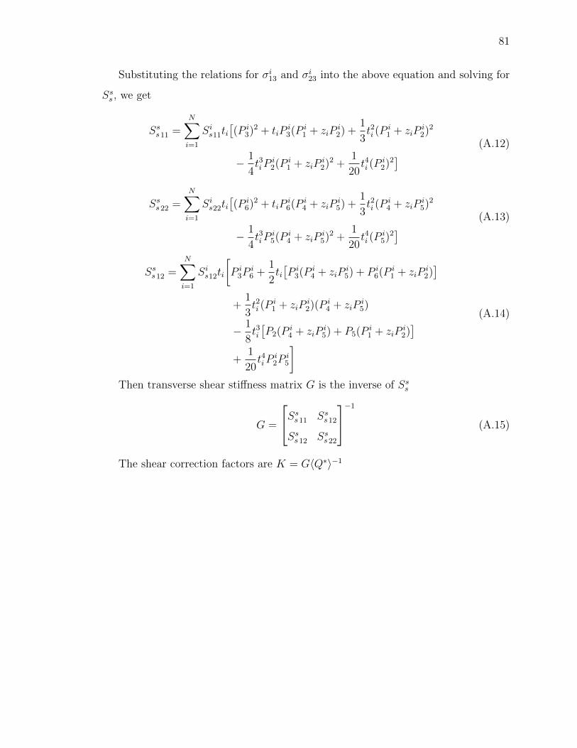
81
Substituting the relations for σi13 and σi23 into the above equation and solving for
Sss , we get
Sss11 =N∑i=1
Sis11ti[(P i
3)2 + tiPi3(P i
1 + ziPi2) +
1
3t2i (P
i1 + ziP
i2)2
− 1
4t3iP
i2(P i
1 + ziPi2)2 +
1
20t4i (P
i2)2] (A.12)
Sss22 =N∑i=1
Sis22ti[(P i
6)2 + tiPi6(P i
4 + ziPi5) +
1
3t2i (P
i4 + ziP
i5)2
− 1
4t3iP
i5(P i
4 + ziPi5)2 +
1
20t4i (P
i5)2] (A.13)
Sss12 =N∑i=1
Sis12ti
[P i
3Pi6 +
1
2ti[P i
3(P i4 + ziP
i5) + P i
6(P i1 + ziP
i2)]
+1
3t2i (P
i1 + ziP
i2)(P i
4 + ziPi5)
− 1
8t3i[P2(P i
4 + ziPi5) + P5(P i
1 + ziPi2)]
+1
20t4iP
i2P
i5
](A.14)
Then transverse shear stiffness matrix G is the inverse of Sss
G =
Sss11 Sss12
Sss12 Sss22
−1
(A.15)
The shear correction factors are K = G〈Q∗〉−1

82

83
B. ANSYS-SWIFTCOMP GUI
To facilitate the use of SwiftCompTM, a simple graphic user interface (GUI) based on
ANSYS, called ANSYS-SwiftComp GUI [19] is developed, which can be downloaded
from cdmHUB: https://cdmhub.org/resources/1136 . The development of this GUI
uses two languages, i.e., ANSYS Parametric Design Language (APDL) and User
Interface Design Language (UIDL). The ANSYS-SwiftComp GUI is modified from
the ANSYS-VAMUCH GUI developed by Zheng Ye and part of the macros are also
inherited from ANSYS-VABS GUI [28] developed by Fang Jiang. Both ANSYS-
VAMUCH GUI and ANSYS-VABS GUI are superseded by ANSYS-SwiftComp GUI.
B.1 ANSYS-SwiftComp GUI Overview
ANSYS-SwiftComp GUI is a graphic user interface integrated in the Main Menu
of ANSYS, which can use the preprocessing and postprocessing capability of ANSYS
as a user friendly GUI for SwiftCompTM. The newly added functions specific for
SwiftCompTM are located in the Preprocessor menu and the Solution menu in ANSYS
as shown in Figure B.1. The functions including Common SGs, Homogenization
and Dehomogenization are completely new to ANSYS and will be explained in the
following:
The first level menu of ANSYS-SwiftComp GUI composes of three major menus:
Preprocessor, Solution and General Postproc.
Preprocessor menu
Material Props: Users can define isotropic, orthotropic or general anisotropic ma-
terial properties under this menu by using Material Models function.
Modeling: Users can build their own models by elementary entities which contain
all basic geometry elements (e.g. point, line, surface, and volume).

84
Figure B.1. Customized menu structure of ANSYS-SwiftComp GUI
Common SGs: Users can create their model through Common SGs, which pro-
vides several common fundamental building blocks of composite materials and struc-
tures.
Mesh: Generate mesh according to the geometry of model, and user can choose
different mesh algorithms to meet their needs.
Solution menu
Homogenization: Users can invoke SwiftCompTM to compute the effect properties
for different structural models (beams, plates/shells or 3D structures).
Dehomogenization: After providing the global behavior, users can invoke SwiftCompTM
to compute the local fields including displacements, stresses and strains, and contour
plots will be automatically generated after calculation is completed.
General Postproc menu
Plot Results: After Dehomogenization, users can choose different contour plots
(displacements, stresses and strains) in this menu to visualize the results.

85
B.2 Create Common SGs
ANSYS-SwiftComp GUI provides a convenient way to create some common SG
models. Engineers can easily create the geometry and mesh of these models, and
invoke SwiftCompTM to perform homogenization and dehomogenization for different
composites with arbitrary fundamental building blocks (aka SGs).
Currently, ANSYS-SwiftComp GUI provides the following common SGs:
1D SGs: layered materials, laminates.
2D SGs: square pack microstructures (with interphase region), hexagonal pack
microstructures (with interphase region).
3D SGs: square pack microstructures, spherical inclusion microstructures.
This appendix mainly focuses on introducing 1D and 2D common SGs for plates/shells
model as this thesis only uses 1D and 2D SGs. For 3D or even customized SGs,
please refer to ANSYS-SwiftComp GUI manual, which can be downloaded from
cdmHUB [19].
There are three different ways to generate 1D SGs for laminates. The fastest way
to generate 1D SG for laminate is to use Fast Generate function: Preprocessor →
Common SG → 1D SGs → Fast Generate. Users can use simple notation to define
ply sequence from the bottom to the top. For example, case 2 uses the notation
[0/90/45/-45/30/-30/75/-75] to indicate ply sequence. Choose the material number
for each lamina and assign thickness for each ply as shown in Figure B.2. Both case
1 and case 2 use Fast Generate function. Note: for Solid Model, 2-noded elements
will be sufficient. And for Plate/Shell Model, 5-noded elements are needed.
After inputting all the parameters, click OK. The 1D SG for the laminate of case
2 has been created as shown in Figure B.3. Note that Fast Generate function only
deals with constant layer thickness and single material property. As shown in Figure
B.3, each layer with five nodes has been shown by five different color lines.
If users want to create laminates with different layer thickness and material prop-
erty, Advanced Generate function in 1D SGs can serve this purpose. Preprocessor→

86
Figure B.2. Fast Generate function
1
X Y
Z
1D SG , Number of layers=8
1
X Y
Z
1D SG , Number of layers=8
PLOT NO. 1
L-K
Figure B.3. 1D SG for case 2
Common SG → 1D SGs → Advanced Generate. Choose a laminate [0/90/45/-45]
with thickness 0.01 as an example, the input parameters for this laminate is shown
in Figure B.4.
In addition, the function of 1D SGs also provides Input File function to let users
upload their own data file. This function can handle laminates with complex ply
sequence. Click Input File function in the 1D SGs menu. Preprocessor → Common
SG → 1D SGs → Input File. A new window will pop out. Users can choose the

87
Figure B.4. 1D SG for case 2
file which contains laminate data. The format of the data file is discussed in the
ANSYS-SwiftComp GUI Manual. The case 3 uses Input File function to generate the
corresponding 1D SG.
The fastest ways to generate common 2D SGs is to use 2D SGs menu: Preprocessor
→ Common SGs → 2D SGs. For example, if we want to create a square pack
microstructure. Choose Square Pack function in 2D SGs menu. Input volume fraction
of fiber and keep volume fraction of interphase empty or zero if there is no interphase
region in your model. Select corresponding material number for the fiber and matrix.
If there is no interphase, keep the Material # for Interphase empty or zero. Select
element type and mesh size as shown in Figure B.5. Click OK, The 2D SG represented
as a square with a circle in the center will be shown in Figure B.6.
B.3 Homogenization and Dehomogenization
After creating SGs, users can perform homogenization and dehomogenization in
ANSYS-SwiftComp GUI, which is explained in the following
Homogenization
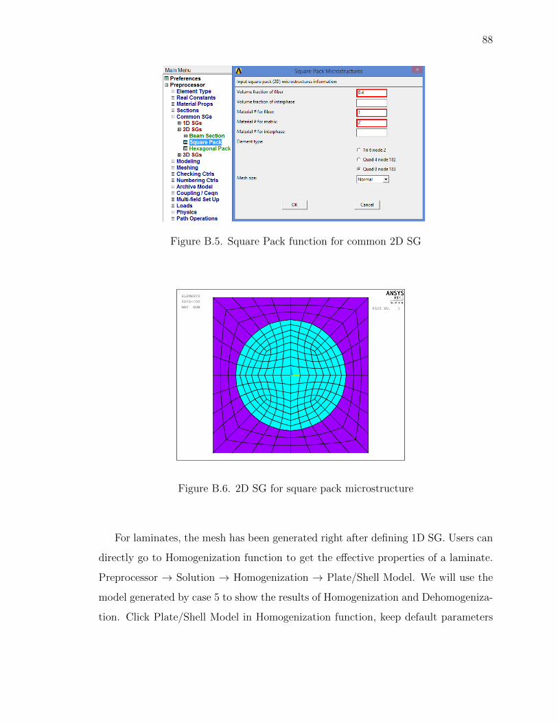
88
Figure B.5. Square Pack function for common 2D SG
1
X Y
Z
PLOT NO. 1
ELEMENTS
DSYS=100
MAT NUM
Figure B.6. 2D SG for square pack microstructure
For laminates, the mesh has been generated right after defining 1D SG. Users can
directly go to Homogenization function to get the effective properties of a laminate.
Preprocessor → Solution → Homogenization → Plate/Shell Model. We will use the
model generated by case 5 to show the results of Homogenization and Dehomogeniza-
tion. Click Plate/Shell Model in Homogenization function, keep default parameters
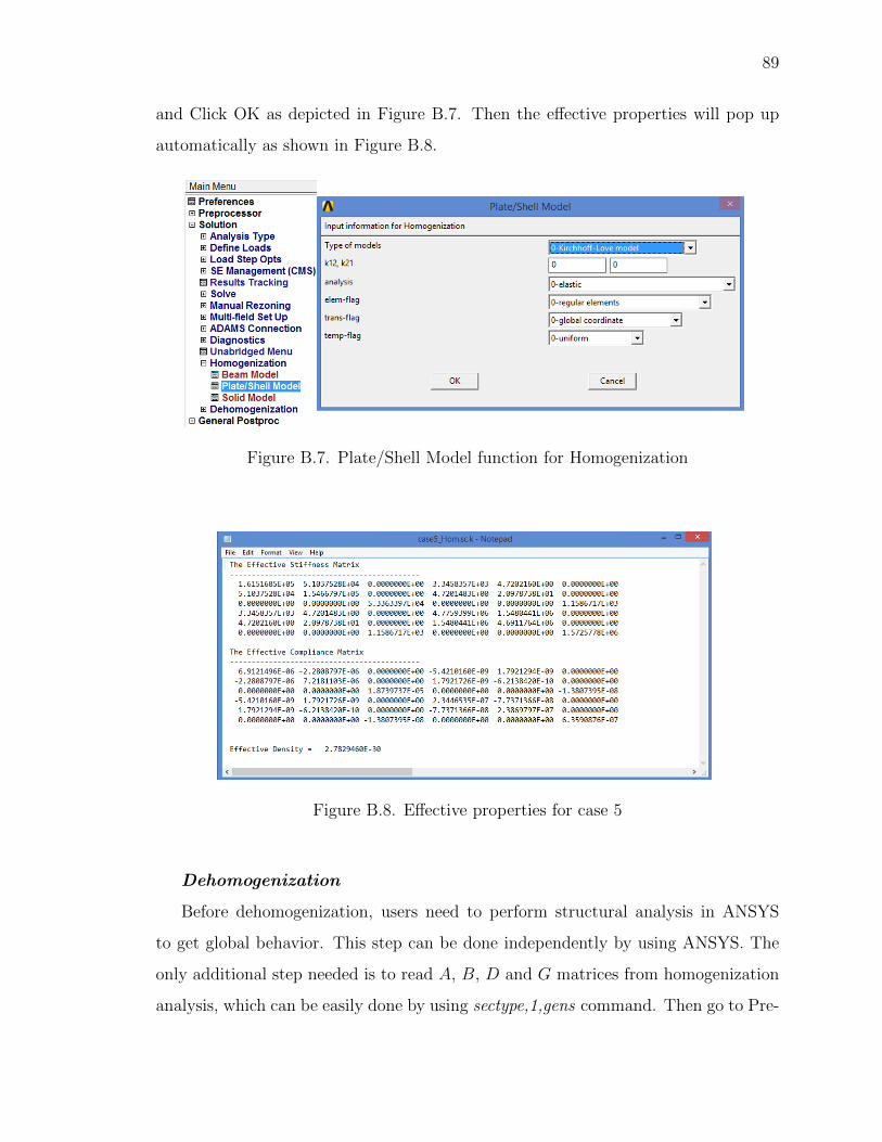
89
and Click OK as depicted in Figure B.7. Then the effective properties will pop up
automatically as shown in Figure B.8.
Figure B.7. Plate/Shell Model function for Homogenization
Figure B.8. Effective properties for case 5
Dehomogenization
Before dehomogenization, users need to perform structural analysis in ANSYS
to get global behavior. This step can be done independently by using ANSYS. The
only additional step needed is to read A, B, D and G matrices from homogenization
analysis, which can be easily done by using sectype,1,gens command. Then go to Pre-
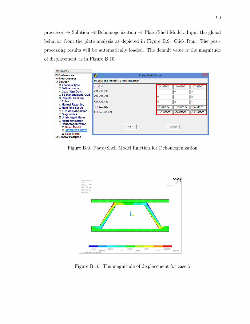
90
processor → Solution → Dehomogenization → Plate/Shell Model. Input the global
behavior from the plate analysis as depicted in Figure B.9. Click Run. The post-
processing results will be automatically loaded. The default value is the magnitude
of displacement as in Figure B.10.
Figure B.9. Plate/Shell Model function for Dehomogenization
1
MNMX
X Y
Z
2D Structure Genome
.182901
.182941
.182981
.183021
.18306
.1831
.18314
.18318
.183219
.183259
PLOT NO. 1
NODAL SOLUTION
SUB =1
USUM (AVG)
RSYS=SOLU
DMX =.183259
SMN =.182901
SMX =.183259
DSYS=100
Figure B.10. The magnitude of displacement for case 5