Analysis of Composite Aerospace StructuresFinite Elements Professor Kelly

John Middendorf #3049731Assignment #3

I hereby certify that this is my own and original work.Signed,

John Middendorf

Analysis ObjectiveUsing a composite material, an airfoil is to be analyzed in Patran/Nastran with the following dimensions and design requirements.

Loads and Boundary ConditionsThe airfoil is subjected to a upward pressure load of 10kPa on the top surface, and fixed by six points on the rear spar.

Composite MaterialThe composite consists of 8 layers of 0.2mm thick pre-preg composite fabric modeled as a 2D orthotropic material with the properties as shown on the right:

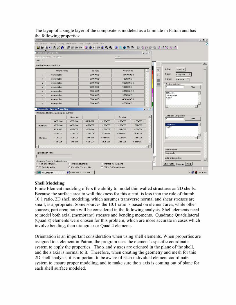
The layup of a single layer of the composite is modeled as a laminate in Patran and has the following properties:

Shell ModelingFinite Element modeling offers the ability to model thin walled structures as 2D shells. Because the surface area to wall thickness for this airfoil is less than the rule of thumb 10:1 ratio, 2D shell modeling, which assumes transverse normal and shear stresses are small, is appropriate. Some sources the 10:1 ratio is based on element area, while other sources, part area; both will be considered in the following analysis. Shell elements need to model both axial (membrane) stresses and bending moments. Quadratic Quadrilateral (Quad 8) elements were chosen for this problem, which are more accurate in cases which involve bending, than triangular or Quad 4 elements.

Orientation is an important consideration when using shell elements. When properties are assigned to a element in Patran, the program uses the element’s specific coordinate system to apply the properties. The x and y axes are oriented in the plane of the shell, and the z axis is normal to it. Therefore, when creating the geometry and mesh for this 2D shell analysis, it is important to be aware of each individual element coordinate system to ensure proper modeling, and to make sure the z axis is coming out of plane for each shell surface modeled.

Model GeometryThree groups were created in Patran, one for the spars and ribs, one for the top surface and one for the bottom surface. Each segment was modeled as an individual surface to ensure proper meshing at each junction (as opposed to joining adjacent co-planar surfaces). Surface normals were verified for each surface in each group:

ElementsQuad 8 elements were used, and consistent XY orientation was attained by the sequence of the selection of curves to create each surface. This wasn’t completely necessary, since our material has equal properties in the x and y directions. I verified this by running some simple tests with varying configurations on the sample shown (below right), and compared the results with the property-equivalent isotropic material (this sample was fixed on one corner and a pressure load applied on the top surface). The important consideration for correct property association is the element normals, which follow the surface normals.

Note: comparison runs were made with Quad 4 and Tria elements, both of which produced stiffer

result(i.e. less flexural deformation). It was important for this model to err on the side of less stiffness, rather than more. See Appendix.Mesh CreationTwo meshes were studied for the final results, one with a nominal 40mm global edge length, the other with a nominal 20mm global edge length. The default isomesh was used as shown on the right. Nodes were of course equivalenced after each complete mesh creation of each group. Because the results were similar, and also because a finer mesh would have exceeded the rule of thumb element area to thickness ratio of 10:1, the two (40mm and 20mm) meshes were considered adequate for the results.

Fixing the MeshThe default mesh created quite a few elements that were out of range in terms of aspect ratio and skew. These were all located at the trailing edge of the rib surfaces, where a overly stiff model could give poor results. Therefore I went through a process to mend each mesh to model more accurately using the following steps:

1. Create the mesh for the ribs and spars.

2. Fix the bad elements by splitting them along the longer edge, until all passed the verification test.

3. Mesh the top and bottom surfaces separately with the global edge length.

4. Equivalence the nodes and check to ensure proper mesh connections.

5. Assign properties and run model.

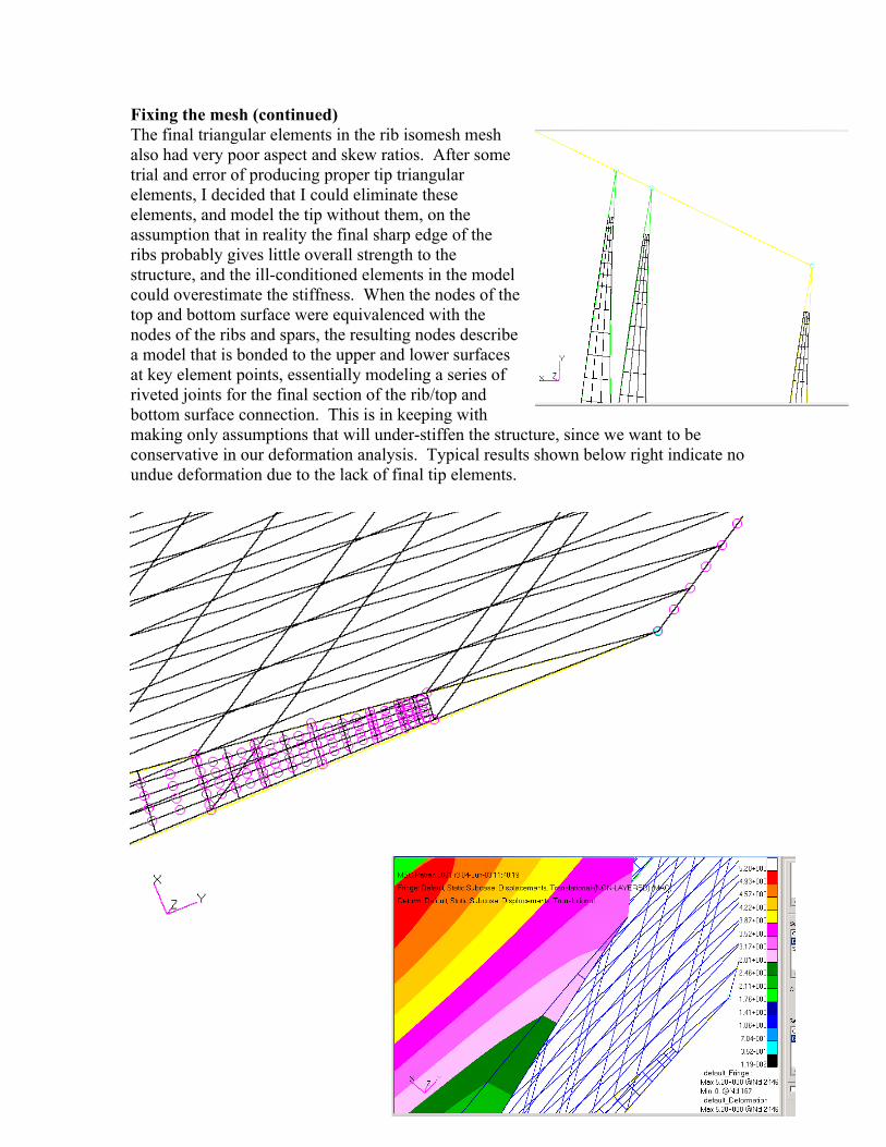
Fixing the mesh (continued)The final triangular elements in the rib isomesh mesh also had very poor aspect and skew ratios. After some trial and error of producing proper tip triangular elements, I decided that I could eliminate these elements, and model the tip without them, on the assumption that in reality the final sharp edge of the ribs probably gives little overall strength to the structure, and the ill-conditioned elements in the model could overestimate the stiffness. When the nodes of the top and bottom surface were equivalenced with the nodes of the ribs and spars, the resulting nodes describe a model that is bonded to the upper and lower surfaces at key element points, essentially modeling a series of riveted joints for the final section of the rib/top and bottom surface connection. This is in keeping with making only assumptions that will under-stiffen the structure, since we want to be conservative in our deformation analysis. Typical results shown below right indicate no undue deformation due to the lack of final tip elements.

Results: Single Layer of Composite Material

Above: One layer of composite deformation fringe. Below: Trailing edge tip deflection XY plot.

Even with one layer of composite, the design meets the tip deflection requirement of 25mm. The 2mm panel deflection relative to the edge is another story. Here the “bubble” dimension it is clearly greater than 2mm.

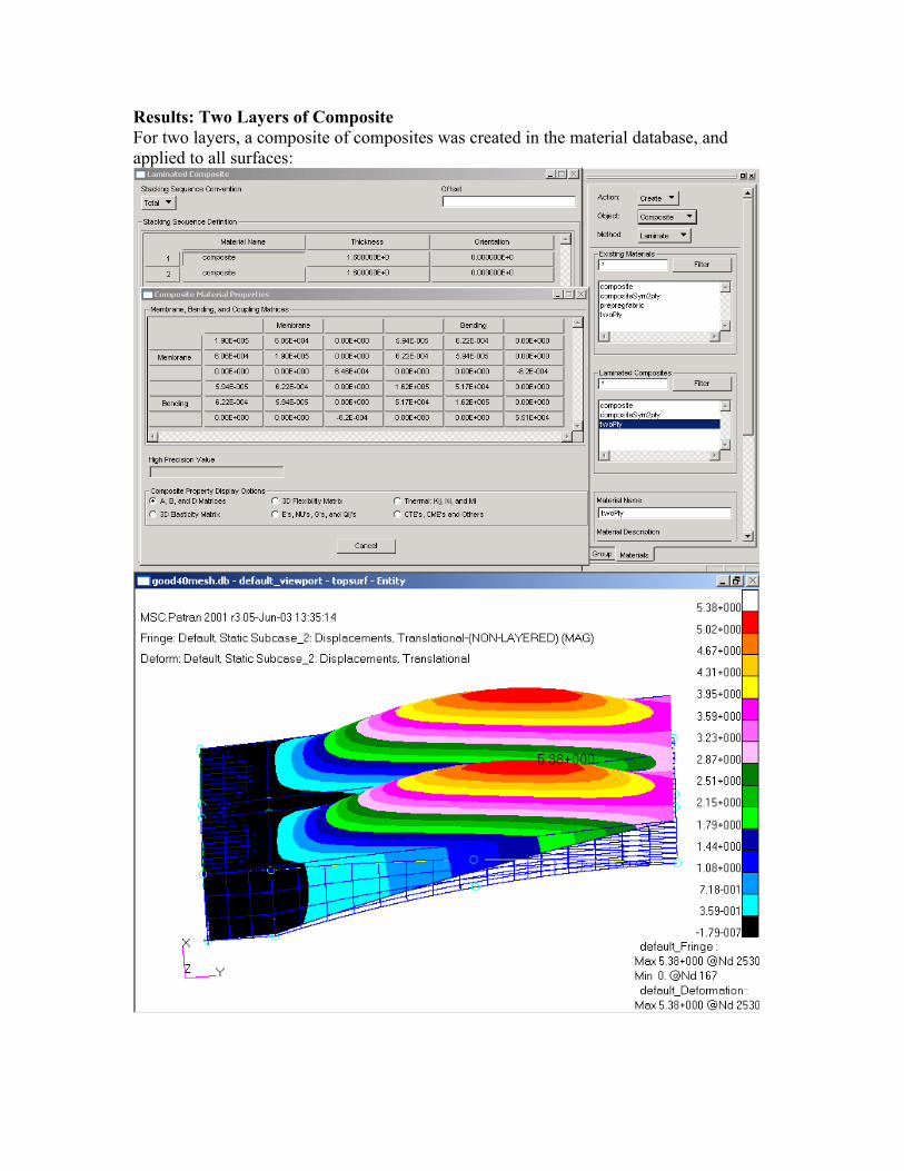
Results: Two Layers of CompositeFor two layers, a composite of composites was created in the material database, and applied to all surfaces:

Results: Two layers (continued)On the right is the tip deflection for the solution with two layers of the composite laminate, with the 40mm mesh.

The bubble dimension is not as easy to determine as the tip deflection. Because of the deflected angle of the airfoil, the maximum height of the bubble does not correspond to the maximum displacement given by the deformation fringe result.

The actual distance of the height of the bubble form the edge is relative to the deformed edge profile. In the XY graph below left, it is relative to the difference between the upper curve, which is plotting the y values for deformation along the line that goes through the point of maximum deformation, and the lower curve, which is the deformation plot of the edge of the airfoil (measured at the top edge of an end rib). The actual value of the height of the bubble can be found by multiplying the difference between the two curves by the cosine of the deflection angle. The deflection angle is approximately 0.27 (the arctan of 3.3/700), the cosine of which is essentially 1 (0.9999). After going through the mathematics of how to calculate the equivalent edge deformation in the deflected state from the XY values of the original state, it was decided to approximate maximum bubble deformation. Here, for the two ply, reading off the XY plot below, it is about 5.3mm-1.5mm= 3.8 mm.

Bubble EstimationIn order to estimate the bubble, I also tried fixing the bottom surface of the ribs, which gave the following results:

Above: Fixed bottom center spar edges. Above right: tip deflection for fixed spar run. These results seem to underestimate the actual bubble height, in addition, the center top surface panel is pulled up by the upward pressure, rather than deflecting downward as in the normal run with only the control surfaces fixed.

In any case, two layers of composite layup does not meet the 2mm bubble deflection requirement. On to three layers, next.

Results: Three layers of composite.

Above: Deformation Fringe plot with three layers of composite. Left: Tip deformation XY plot.

Three Layer Analysis

Again, fixing the bottom spars gives us a rough idea of the bubble deflection:

But more accurate numbers come from reading the graph plotting the end rib top edge deflection and the center line of the maximum deflection curve:

Here, the maximum value of the bubble height to be around 2.65-0.9=1.75mm, which meets the 2mm requirement. Therefore, 3 layers of laminate material are required.

Results: 20 mm mesh run to confirm result of coarse mesh:

The finer mesh confirms the coarse mesh results (where max deformation was 2.56). Maximum bubble is again around 2.65-0.9 = 1.75mm. This is a conservative estimate, but three layers of composite layup meets all requirements for the problem. ANSWER: Three layers of composite required.

Bonus PagesShape of Final Deformation (three layers of laminate)

Four Layer Solution:

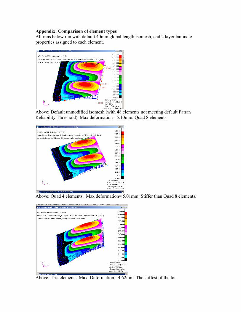
Appendix: Comparison of element typesAll runs below run with default 40mm global length isomesh, and 2 layer laminate properties assigned to each element.

Above: Default unmodified isomesh (with 48 elements not meeting default Patran Reliability Threshold). Max deformation= 5.10mm. Quad 8 elements.

Above: Quad 4 elements. Max deformation= 5.01mm. Stiffer than Quad 8 elements.

Above: Tria elements. Max. Deformation =4.62mm. The stiffest of the lot.