analysis of complex bursting patterns in multiple
TRANSCRIPT

ANALYSIS OF COMPLEX BURSTING PATTERNS IN
MULTIPLE TIMESCALE RESPIRATORY NEURON
MODELS
by
Yangyang Wang
B.S., Applied Mathematics, Beijing Normal University, 2010
Submitted to the Graduate Faculty of
the Kenneth P. Dietrich School of Arts and Sciences in partial
fulfillment
of the requirements for the degree of
Doctor of Philosophy
University of Pittsburgh
2016
UNIVERSITY OF PITTSBURGH
DIETRICH SCHOOL OF ARTS AND SCIENCES
This dissertation was presented
by
Yangyang Wang
It was defended on
May 3rd 2016
and approved by
Jonathan E. Rubin, Department of Mathematics
G. Bard Ermentrout, Department of Mathematics
Brent Doiron, Department of Mathematics
David M. Jasnow, Department of Physics and Astronomy
Dissertation Director: Jonathan E. Rubin, Department of Mathematics
ii

ANALYSIS OF COMPLEX BURSTING PATTERNS IN MULTIPLE TIMESCALE
RESPIRATORY NEURON MODELS
Yangyang Wang, PhD
University of Pittsburgh, 2016
Many physical systems feature interacting components that evolve on disparate timescales. Signif-
icant insights about the dynamics of such systems have resulted from grouping timescales into two
classes and exploiting the timescale separation between classes through the use of geometric sin-
gular perturbation theory. It is natural to expect, however, that some dynamic phenomena cannot
be captured by a two timescale decomposition. One example is the mixed burst firing mode, ob-
served in both recordings and model pre-Botzinger neurons, which appears to involve at least three
timescales based on its time course. With this motivation, we construct a model system consisting
of a pair of Morris-Lecar systems coupled so that there are three timescales in the full system.
We demonstrate that the approach previously developed in the context of geometric singular per-
turbation theory for the analysis of two timescale systems extends naturally to the three timescale
setting. To elucidate which characteristics truly represent three timescale features, we investigate
certain reductions to two timescales and the parameter dependence of solution features in the three
timescale framework. Furthermore, these analyses and methods are extended and applied to under-
stand multiple timescale bursting dynamics in a realistic single pre-Botzinger complex neuron and
a heterogeneous population of these neurons, both of which can generate a novel mixed bursting
(MB) solution, also observed in pre-BotC neuron recordings. Rather surprisingly, we discover that
a third timescale is not actually required to generate mixed bursting solution in the single neuron
model, whereas at least three timescales should be involved in the latter model to yield a simi-
lar mixed bursting pattern. Through our analysis of timescales, we also elucidate how the single
pre-BotC neuron model can be tuned to improve the robustness of the MB solution.
iii

Keywords: fast-slow systems, multiple timescales, oscillations, geometric singular perturbation
theory, bursting, respiratory neuron, persistent sodium, calcium.
iv

TABLE OF CONTENTS
PREFACE . . . . . . . . . . . . . . . . . . . . . . . . . . . . . . . . . . . . . . . . . xiii
1.0 INTRODUCTION . . . . . . . . . . . . . . . . . . . . . . . . . . . . . . . . . . . . 1
1.1 Generation of respiratory rhythms . . . . . . . . . . . . . . . . . . . . . . . . . . 1
1.2 Models of respiratory rhythm generation in the pre-BotC . . . . . . . . . . . . . . 2
1.3 geometric singular perturbation theory: fast/slow analysis . . . . . . . . . . . . . . 4
1.4 Outline . . . . . . . . . . . . . . . . . . . . . . . . . . . . . . . . . . . . . . . . 8
2.0 UNDERSTANDING AND DISTINGUISHING THREE TIME SCALE OSCIL-
LATIONS: CASE STUDY IN A COUPLED MORRIS-LECAR SYSTEM . . . . . 11
2.1 Preliminaries . . . . . . . . . . . . . . . . . . . . . . . . . . . . . . . . . . . . . 15
2.1.1 Singular limits: scalings and subsystems . . . . . . . . . . . . . . . . . . . . 17
2.1.2 Effect of coupling . . . . . . . . . . . . . . . . . . . . . . . . . . . . . . . 24
2.2 Analysis of three timescale solutions . . . . . . . . . . . . . . . . . . . . . . . . . 28
2.2.1 Case 1: gsyn=1.0 . . . . . . . . . . . . . . . . . . . . . . . . . . . . . . . . 29
2.2.1.1 (v1, w1) driven by (v2, w2) . . . . . . . . . . . . . . . . . . . . . . . 29
2.2.2 Case 2: gsyn=4.1 . . . . . . . . . . . . . . . . . . . . . . . . . . . . . . . . 32
2.2.2.1 (v1, w1) driven by (v2, w2) . . . . . . . . . . . . . . . . . . . . . . . 32
2.2.3 Case 3: gsyn=5.1 . . . . . . . . . . . . . . . . . . . . . . . . . . . . . . . . 36
2.2.3.1 (v1, w1) driven by (v2, w2) . . . . . . . . . . . . . . . . . . . . . . . 36
2.3 Identifying three timescale features . . . . . . . . . . . . . . . . . . . . . . . . . . 38
2.3.1 gsyn = 1.0: recruitment of a transient V1 spike . . . . . . . . . . . . . . . . . 39
2.3.2 gsyn = 4.1: transition from V1 spikes of gradually decaying amplitude to V1
spikes of constant amplitude . . . . . . . . . . . . . . . . . . . . . . . . . . 42
v

2.3.3 gsyn = 5.1: direct transition to a depolarized plateau . . . . . . . . . . . . . 45
2.4 Discussion . . . . . . . . . . . . . . . . . . . . . . . . . . . . . . . . . . . . . . . 47
3.0 MULTIPLE TIMESCALE MIXED BURSTING DYNAMICS IN A RESPIRA-
TORY NEURON MODEL . . . . . . . . . . . . . . . . . . . . . . . . . . . . . . . . 52
3.1 Analysis of the mixed bursting model . . . . . . . . . . . . . . . . . . . . . . . . 56
3.1.1 Rescaling and simplification of timescales . . . . . . . . . . . . . . . . . . . 58
3.1.2 Dynamics of the constant-τ model (3.5) . . . . . . . . . . . . . . . . . . . . 61
3.1.3 Finding the combination of timescales that supports MB solutions in the
constant-τ model (3.5) . . . . . . . . . . . . . . . . . . . . . . . . . . . . . 65
3.1.3.1 (C1)⇒ Analysis of timescales of v and n . . . . . . . . . . . . . . . 65
3.1.3.2 (C2) and (C3)⇒ Analysis of timescales of h, v2 and w . . . . . . . 69
3.1.4 Dynamics of the mixed bursting model (3.1) . . . . . . . . . . . . . . . . . 72
3.2 Robustness of the mixed bursting model . . . . . . . . . . . . . . . . . . . . . . . 75
3.2.1 Robustness to [IP3] . . . . . . . . . . . . . . . . . . . . . . . . . . . . . . . 75
3.2.2 Robustness to gNaP . . . . . . . . . . . . . . . . . . . . . . . . . . . . . . . 79
3.3 Discussion . . . . . . . . . . . . . . . . . . . . . . . . . . . . . . . . . . . . . . . 83
4.0 MULTIPLE TIMESCALE SIGH-LIKE BURSTING IN A SELF-COUPLED PRE-
BOTC NEURON . . . . . . . . . . . . . . . . . . . . . . . . . . . . . . . . . . . . . 86
4.1 Analysis of sigh-like bursting . . . . . . . . . . . . . . . . . . . . . . . . . . . . . 91
4.1.1 Mechanisms underlying regular bursting . . . . . . . . . . . . . . . . . . . . 95
4.1.2 Mechanisms underlying the transition from regular bursts to the sigh-like burst 97
4.2 Identifying timescales . . . . . . . . . . . . . . . . . . . . . . . . . . . . . . . . . 105
4.3 Discussion . . . . . . . . . . . . . . . . . . . . . . . . . . . . . . . . . . . . . . . 107
5.0 CONCLUSIONS . . . . . . . . . . . . . . . . . . . . . . . . . . . . . . . . . . . . . 111
5.1 Summary . . . . . . . . . . . . . . . . . . . . . . . . . . . . . . . . . . . . . . . 111
5.2 When do we need three timescales? . . . . . . . . . . . . . . . . . . . . . . . . . 113
5.3 Analysis of 3 timescale systems . . . . . . . . . . . . . . . . . . . . . . . . . . . 114
6.0 APPENDIX . . . . . . . . . . . . . . . . . . . . . . . . . . . . . . . . . . . . . . . . 117
6.1 Nondimensionalization of the coupled Morris-Lecar system . . . . . . . . . . . . . 117
6.2 Adjusting timescales in the dendritic subsystem . . . . . . . . . . . . . . . . . . . 118
vi

6.3 Nondimensionalization of the mixed bursting model . . . . . . . . . . . . . . . . . 119
6.4 Nondimensionalization of the Jasinski model . . . . . . . . . . . . . . . . . . . . 123
BIBLIOGRAPHY . . . . . . . . . . . . . . . . . . . . . . . . . . . . . . . . . . . . . . . 125
vii

LIST OF TABLES
2.1 The values of the parameters in the model given by (2.1) and (2.2). . . . . . . . . . 13
2.2 Subsystems for (2.4). . . . . . . . . . . . . . . . . . . . . . . . . . . . . . . . . . 22
3.1 The values of the parameters in the pre-BotC model given by equations (3.1) and
(3.2) . . . . . . . . . . . . . . . . . . . . . . . . . . . . . . . . . . . . . . . . . . 54
3.2 Timescales for the constant-τ model (3.5) . . . . . . . . . . . . . . . . . . . . . . . 72
3.3 Time Scales of n and h . . . . . . . . . . . . . . . . . . . . . . . . . . . . . . . . 74
4.1 Ionic currents and channel reversal potentials . . . . . . . . . . . . . . . . . . . . . 88
4.2 Activation and inactivation variables . . . . . . . . . . . . . . . . . . . . . . . . . 88
4.3 Activation and inactivation variables . . . . . . . . . . . . . . . . . . . . . . . . . 89
5.1 Subsystems for 3 timescale system. . . . . . . . . . . . . . . . . . . . . . . . . . . 115
6.1 The timescales for the Jasinski model. . . . . . . . . . . . . . . . . . . . . . . . . 124
viii

LIST OF FIGURES
1.1 Schematic diagram showing construction of a singular periodic orbit by concatena-
tion of solution segments for singular limit systems. . . . . . . . . . . . . . . . . . 7
1.2 Typical fast/slow analysis (with h slow and V fast) for square-wave bursting. . . . . 9
2.1 Baseline phase planes for the two ML systems without coupling. . . . . . . . . . . 14
2.2 Time series for attracting solutions of (2.1)-(2.2) with parameter values as in Ta-
ble 2.1 and with the indicated values of gsyn. . . . . . . . . . . . . . . . . . . . . . 16
2.3 Nullclines for v1 (red) and w1 (cyan) for the v2-frozen system (2.19). . . . . . . . . 25
2.4 Bifurcation diagrams for (2.19) with v2 as a parameter. . . . . . . . . . . . . . . . . 25
2.5 Bifurcation curves for (2.19) in (v2, gsyn) parameter space. . . . . . . . . . . . . . . 26
2.6 Graph of S(v2) (blue) and locus of the v2-nullcline (black/red). . . . . . . . . . . . 27
2.7 Attracting dynamics in (v2, w2)-space. . . . . . . . . . . . . . . . . . . . . . . . . 28
2.8 An attracting solution of (2.4) for gsyn = 1.0 (black curve) projected to the (v1, w1)
plane. . . . . . . . . . . . . . . . . . . . . . . . . . . . . . . . . . . . . . . . . . . 30
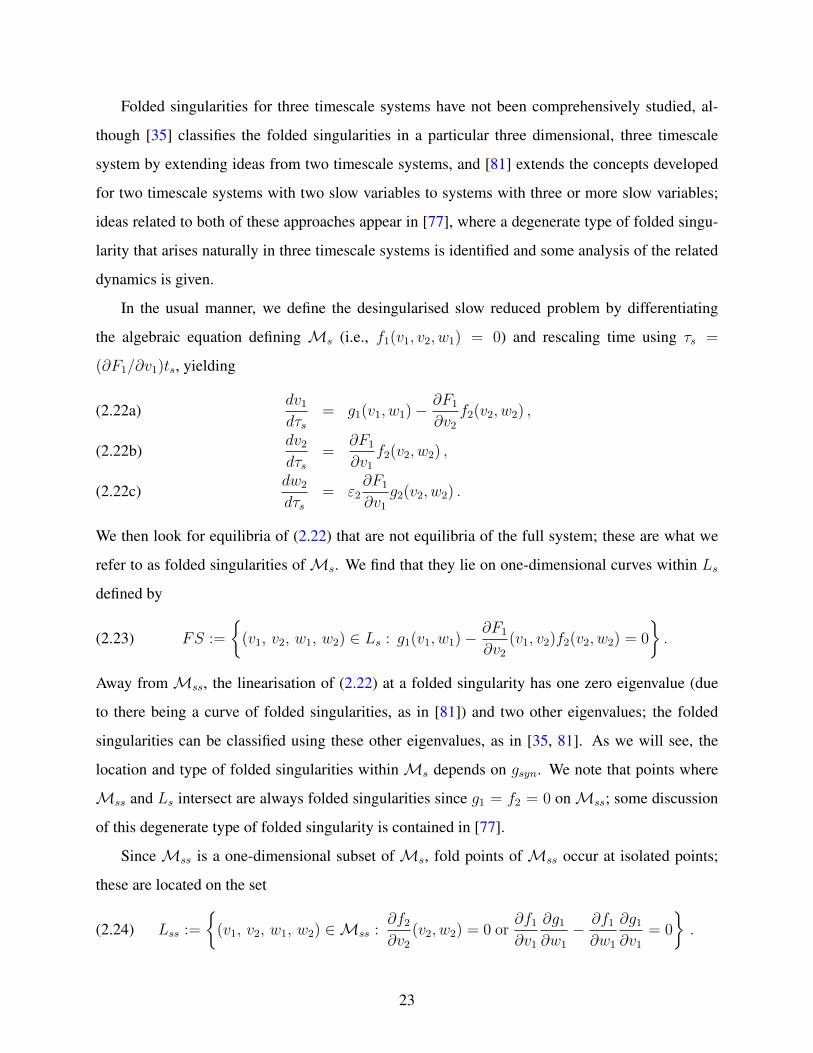
2.9 The attracting trajectory from Figure 2.8 (black curve) projected onto the (w1, v2)
plane. . . . . . . . . . . . . . . . . . . . . . . . . . . . . . . . . . . . . . . . . . . 31
2.10 An attracting solution of (2.4) for gsyn = 4.1, projected to (v1, w1)-space (black
curve). . . . . . . . . . . . . . . . . . . . . . . . . . . . . . . . . . . . . . . . . . 34
2.11 Projection to the (w1, v2)-plane illuminates several features of the periodic solution
(black) for gsyn = 4.1. . . . . . . . . . . . . . . . . . . . . . . . . . . . . . . . . . 35
2.12 An attracting solution of (2.4) for gsyn = 5.1, projected to (v1, w1)-space (black
curve), together with nullclines for (2.19). Colours of curves are as in Figure 2.10. . 36
ix

2.13 Projection to the (w1, v2) plane illuminates several features of the periodic solution
(black) for gsyn = 5.1. . . . . . . . . . . . . . . . . . . . . . . . . . . . . . . . . . 37
2.14 Projections of solutions for gsyn = 1.0 onto (V1, V2, w2)-space. . . . . . . . . . . . 39
2.15 Time series of rescaled versions of (2.1) with gsyn = 1.0. . . . . . . . . . . . . . . . 40
2.16 Time series of (2.1) with gsyn = 4.1. . . . . . . . . . . . . . . . . . . . . . . . . . 42
2.17 Time courses of V2 (red) and V1 (black/blue/green) . . . . . . . . . . . . . . . . . . 43
2.18 Projection of the attracting solution (black curve) of the (3S, 1SS) system with
gsyn = 4.1, C1 = 80, φ2 = 0.0001 onto (V1, V2, w2)-space. Red curves denote
Mss, and blue and green circles mark two folds ofMss. . . . . . . . . . . . . . . 45
2.19 Time series of (2.1) with gsyn = 5.1. . . . . . . . . . . . . . . . . . . . . . . . . . 46
3.1 Basic structures of the two subsystems (3.1a)-(3.1c) and (3.1d)-(3.1e) with param-
eter values as given in Table 3.1 but without coupling. . . . . . . . . . . . . . . . . 54
3.2 Time series for bursting solutions of the full system (3.1)-(3.2). . . . . . . . . . . . 56
3.3 Attracting dynamics in ([Ca], l)-space. . . . . . . . . . . . . . . . . . . . . . . . . 57
3.4 Functions (A) 1/τn(V ) and (B) 1/τh(V ). Note the difference in vertical scales
between panels. . . . . . . . . . . . . . . . . . . . . . . . . . . . . . . . . . . . . 59
3.5 Simulation of the MB solution generated by (3.5), together with corresponding bi-
furcation diagrams. . . . . . . . . . . . . . . . . . . . . . . . . . . . . . . . . . . 62
3.6 Bifurcation diagrams for the somatic subsystem for various τn values. . . . . . . . . 66
3.7 Bifurcation curves for the (v, n) subsystem of (3.5) for c = 0. . . . . . . . . . . . . 69
3.8 Time series for attracting solutions of the constant-τ model and associated bifurca-
tion diagrams when Rv = 1, Rn = 5, Rc = 10, and Rl = 1000. . . . . . . . . . . . 71
3.9 The graphs of the functions 1/τn(v) and 1/τh(v), with both default and new choices
of σn, an, σh and ah. . . . . . . . . . . . . . . . . . . . . . . . . . . . . . . . . . . 73
3.10 The bifurcation diagrams of the somatic subsystem corresponding to the modified
forms of τn(v) as shown in Figure 3.9A, along with the h-nullcline (cyan). The
other color codings are the same as in Figure 3.9A. . . . . . . . . . . . . . . . . . . 74
3.11 Time series for attracting solutions of (3.4) and corresponding bifurcation diagrams. 76
3.12 Regions of MB solutions for the mixed bursting model. . . . . . . . . . . . . . . . 77
x

3.13 Time series of (3.4) with Cm = 21, KCa = 1.25 × 10⁻⁴, A = 0.001, σn = −5 ,
an = 0.1, σh = 7 and ah = 0.001. . . . . . . . . . . . . . . . . . . . . . . . . . . . 77
3.14 Projection of the two MB solutions (black) from Figure 3.13 to (c, l)-space. . . . . . 79
3.15 Bifurcations of the dendritic subsystem. . . . . . . . . . . . . . . . . . . . . . . . . 80
3.16 The zoomed view of two-parameter bifurcation diagrams of HC (red), LF (blue)
and the trajectory (black) from Figure 3.13, projected into (h, gCANtot)-space. . . . . 81
3.17 Two curves of HC bifurcations and two overlapping curves of LF bifurcations, in
(h, gCANTot) parameter space. . . . . . . . . . . . . . . . . . . . . . . . . . . . . . 81
3.18 Effect of variations in gNaP on the behaviors of the somatic subsystem. . . . . . . . 82
3.19 Spiking/bursting and bursting/plateauing boundaries of the somatic subsystem. . . . 83
4.1 Mixed bursting solution (A) and sigh-like bursting solution (B) from [80] and [30],
respectively. . . . . . . . . . . . . . . . . . . . . . . . . . . . . . . . . . . . . . . 87
4.2 Simulation of sigh-like rhythmic bursting of the Jasinski model. . . . . . . . . . . . 91
4.3 Basic structures of the voltage subsystem (4.1a)-(4.1d) and the calcium subsystem
(4.1e)-(4.1g). . . . . . . . . . . . . . . . . . . . . . . . . . . . . . . . . . . . . . . 94
4.4 Bifurcation diagrams of the Fast system (4.1a)-(4.1c) with the slow variables Nai
and Cai taken as static parameters. . . . . . . . . . . . . . . . . . . . . . . . . . . 96
4.5 Effect of variations in Catot on the trajectories of the fast-slow subsystem (V, y,Cai,Nai)
for l = 0.94. . . . . . . . . . . . . . . . . . . . . . . . . . . . . . . . . . . . . . . 99
4.6 Averaged phase planes, corresponding to (4.2), with superimposed trajectories of
the Fast-Slow system, for l = 0.94 and three different values of Catot as in Figure
4.5. . . . . . . . . . . . . . . . . . . . . . . . . . . . . . . . . . . . . . . . . . . . 101
4.7 Bifurcation diagram of the average slow system (4.2) with respect to Catot with l
fixed at 0.94. . . . . . . . . . . . . . . . . . . . . . . . . . . . . . . . . . . . . . . 102
4.8 Simulation of the SB solution generated by the Jasinski model (4.1), together with
the bifurcation diagrams. . . . . . . . . . . . . . . . . . . . . . . . . . . . . . . . 104
4.9 Rescaled version of (4.1): (9F, 2SS) case, with β = 100, αNa = 5× 10⁻³. . . . . . 107
4.10 Rescaled version of (4.1): (7F, 4SS) case, with β = 0.1, αNa = 5× 10⁻⁶. . . . . . . 108
5.1 Frequency-power plot for V in the MB solution (A) and the SB solution (B). . . . . 113
xi

6.1 Time series for attracting solutions of the full model (3.1) as well as the bifurcation
structure of the dendritic subsystem with parameter values as in Table 3.1. . . . . . 120
xii
PREFACE
First of all, I would like to express my deepest gratitude to my advisor Dr. Jonathan Rubin for
giving me the opportunity to join these exciting research projects. It is you who lead me to this
wonderful world of mathematical neuroscience, and support me to attend conferences and to meet
with collaborators and fellow researchers from all over the world. Also, thank you for bringing me
to New Zealand where I not only made breakthrough in my research but also had the most precious
memories in my life. This work would never be completed without your wisdom, your patience
and your invaluable guidance through these past 5 years.
Besides, I would also like to express my sincerest gratitude to Bard Ermentrout, Brent Doiron
and David Jasnow for serving on my committee and your valuable criticism and advices on shaping
this thesis project; to Hinke Osinga and Bernd Krauskopf for inviting me to visit the University of
Auckland to engage in research discussions on collaborative work in the area of multiple timescale
dynamical systems, which inspired the contents of Chapter 2 of this thesis; to Vivien Kirk and
Pingyu Nan for the wonderful collaboration I have had during my visit to the University of Auck-
land. I will never forget our weekly meeting during my three months’ stay and how we worked
together on the project in Chapter 2; to Theodore Vo and Kerry-Lyn Roberts for teaching me how
to compute bifurcations and averaged nullclines using AUTO.
To my family, thank you for your love and support whenever I feel lost. Without you, none
of my goals would have been achieved. Thank my fiance, Changqing Wang, for your accompany,
encouragement and love. I am so grateful to have you as my partner in my life.
xiii

1.0 INTRODUCTION
1.1 GENERATION OF RESPIRATORY RHYTHMS
Breathing is an essential behavior regulating the oxygen and carbon dioxide in mammals, required
to sustain life. The role of the brain in respiration was accepted in the early nineteenth century [37],
which sets the basis for the investigations into the sites and mechanisms underlying the generation
of respiratory rhythm. One of the earliest results, a classical lesion study on adult cat by Lumsden
(1923) [38], suggested that the neurons in pons are part of the network controlling breathing. In
the 1990s, several studies have suggested that breathing is controlled by a neural central pattern
generator (CPG) consisting of groups of neurons in both pons and medulla regions. Many ponto-
medullary respiratory network models have been developed for understanding the respiratory brain
stem and connectivity between different brainstem compartments [16, 49, 66, 60]. The respiratory
rhythm results from the interactions of neuronal populations distributed within the ventrolateral
respiratory column (VRC) as well as neural populations in other brainstem regions including the
pontine respiratory group (PRG) [1, 62]. The output of the brainstem respiratory network is then
transmitted to motoneurons that drive the respiratory pump muscles located at the spinal cord, e.g.,
motoneurons that contract diaphragm such that the lung expands during inspiration. Recent exper-
iment by [20] on brainstem of goat suggested that there is a clear difference in the role for different
sites but all play an essential role in the control of breathing. Even after all these years of intensive
investigations of the neural network related to respiratory system, the underlying mechanisms for
breathing are still not fully understood and require much effort in the future.
One of the main characteristics of respiration is rhythmicity, and identifying the mechanism for
rhythm generation is a very fundamental step in understanding the neural control of breathing. In
1991, the pre-Botzinger complex (pre-BotC), a subregion of the ventrolateral medulla of the brain-
1

stem, has been firstly discovered by Smith et al to be the primary neuronal kernel for respiratory
rhythm generation [65]. Pacemaker neurons with intrinsic bursting properties have been identified
in this region. In total, there exist two distinct types of intrinsically bursting cells in terms of dif-
ferent underlying ionic mechanisms in pre-BotC. The first is voltage-dependent [65] and based on
the persistent (fast activating and slowly inactivating) Na+ current (INaP) in neurons [7, 8]. The
presence of INaP has been confirmed [44, 43, 22], and pharmacologically blocking INaP could si-
lence the pre-BotC rhythmic activity in medullary slices from neonatal rats [61, 22]. Alternatively,
another type of pacemaker has also been identified [72] and the underlying mechanism depends on
a Ca2+-activated nonspecific cationic current (ICAN) [46].
The demonstration that respiratory-related rhythmic activity in the in vitro slice and en bloc
preparations persists after the blockade of synaptic inhibition [11, 17, 50, 63] leads to the hy-
pothesis that rhythmogenesis results from neurons with pacemaker-like properties. However, the
respiratory CPG, the pre-BotC, still exhibits respiratory rhythmicity after stopping the bursting be-
haviour in both population of INaP and ICAN pacemaker neurons simultaneously [45, 43, 16, 43]. It
is therefore suggested that bursting-pacemaker neurons are not essential for respiratory rhythmoge-
nesis. Alternatively, a group-pacemaker has been proposed as the fundamental unit for respiratory
rhythmogenesis: burst rhythms originate from recurrent synaptic excitation that combine with neu-
rons with intrinsic pacemaker properties [51].
1.2 MODELS OF RESPIRATORY RHYTHM GENERATION IN THE PRE-BOTC
The rhythmic respiratory pattern is complex, even at single neuron level. To describe the behavior
of individual respiratory neurons, Butera et al. [7, 8] developed and analyzed computational mod-
els for individual bursting pacemaker neurons in the pre-BotC as well as heterogeneous populations
of these neurons with mutual excitatory synaptic connections. Two minimal models have been pro-
posed using a Hodgkin-Huxley like formalism, and in the first one, the rhythmic bursting arises
from the persistent (slowly inactivating) Na+ current (INaP). This model matches many experi-
mentally observed properties of pre-BotC neurons. For instance, it has various voltage-dependent
activity states: quiescence at hyperpolarized membrane voltages when INaP is not activated, burst-
2

ing when INaP alternates between activation and inactivation, and tonic spiking activity at more
depolarized voltages where INaP is essentially inactivated. This single cell neuron model has been
widely adopted and used in extensive modeling studies investigating behavior of heterogeneous
excitatory networks of intrinsically and non-intrinsically bursting neurons as a basic model for the
pre-BotC excitatory network [7, 8, 42, 58, 49].
Recall that a Ca2+-activated nonspecific cationic current (ICAN) is also involved in bursting
generated in the pre-BotC neurons. A computational model of bursting activity based on ICAN was
proposed by Rubin et al. [56] based on the group pacemaker hypothesis for inspiratory rhythm
generation, as described before. The role of synaptic mechanisms and network interactions in
generating emergent network rhythms (which cannot be generated by single neurons) has been
emphasized. In this group pacemaker model, the activation of ICAN due to Ca2+ accumulation
triggered by recurrent synaptic excitation initiates a network-wide burst, the termination of which
is relying on transient Na+ current-dependent spike inactivation and the activation of outward
currents, rather than on INaP inactivation.
By combining together these two intrinsic Na+- and Ca2+-dependent mechanisms for single-
neuron bursting, Toporikova and Butera [73] have proposed a two-compartment (somatic-dendritic)
model (TB model) of an isolated pre-BotC neuron incorporating INaP and ICAN as two independent
bursting mechanisms. Bursting in the somatic compartment is produced by INaP as in Butera et al.
model [7, 8], whereas bursting in the dendritic compartment is based on Ca2+ oscillations.
Intracellular Ca2+ in the TB model is confined to a dendritic compartment. Since neurons
in the pre-BotC appear to be electronically compact [14], [42], and the model generates qualita-
tively similar dynamics when reduced to a single compartment, Park and Rubin [47] used such a
reduction and studied a single-compartment model (PR model) of a pre-BotC inspiratory neuron
featuring both NaP and CAN currents, as well as intracellular calcium oscillations that activate
the CAN current.
In both TB and PR models, the two intrinsic bursting mechanisms could coexist and interact
to generate a hybrid bursting pattern. Interestingly, a novel mixed bursting (MB) solution, which
appears to involve at least three timescales based on its time course, results from the interaction
of these two mechanisms [47]. Such irregular bursting patterns have also been observed in other
realistic biological models and in recordings from respiratory CPG neurons as well as subthalamic
3

nucleus (STN) neurons in the basal ganglia (e.g. [3], [30], [14]). While [47] presented a mathemat-
ical analysis explaining relevant bursting mechanisms, based on the NaP current, the CAN current,
or both currents working together, less analysis about mixed bursting patterns was provided and
little consideration was given to identifying how many timescales are truly required to obtain these
solutions or to their robustness. Similar MB solution patterns were also recently observed in a
heterogeneous population of pre-BotC neurons by Jasinski et al. [30].
Many physical quantities have characteristic rates at which they tend to evolve. Identifying
relevant timescales is a useful step in modeling physical systems using any sort of dynamic frame-
work. In mathematical analysis in particular, the timescales in a system of differential equations
are often grouped into a small number of classes, so that limits can be taken and the assumptions of
certain mathematical techniques can be satisfied; the aim is to use knowledge of the limit system(s)
to gain information about behaviour of the original system. Examples of this approach are ubiqui-
tous in the literature, with ideas applicable to systems in which timescales can be grouped into two
classes being particularly well developed. However, there have been fewer reported studies that
analyze dynamics involving evolution on three distinct timescales. Even fewer works have exam-
ined decisions about how to group timescales (for example, whether to use two or three classes),
a decision that can arise both in the mathematical treatment of model systems and in the devel-
opment of mathematical models based on experimental observations. Our goal in this thesis is to
do both of these things, with a focus on a certain minimal model system in Chapter 2, a single
pre-BotC neuron model in Chapter 3, and an excitatory neural network of the pre-BotC neurons in
Chapter 4.
1.3 GEOMETRIC SINGULAR PERTURBATION THEORY: FAST/SLOW ANALYSIS
We first review the regular bursting phenomenon from a mathematical viewpoint. The dynamics of
bursting is characterized by the coexistence of oscillatory and non-oscillatory attractors, alternating
between periods of rapid oscillations and slow silent phase of near steady state resting behavior.
The underlying mathematical structures for bursting phenomena involving multiple timescales are
dynamical systems that are often singularly perturbed [28, 33, 10]:
4

dx
dt= f(x, y, ε)(1.1a)
dy
dt= εg(x, y, ε) ,(1.1b)
where x ∈ Rm is fast, y ∈ Rn is slow, t is the fast time, 0 < ε � 1 is a small perturbation
parameter. The functions f and g are both assumed to be sufficiently smooth.
One technique that has been used to deal with such fast/slow system with great success is
geometric singular perturbation theory (GSPT) [19, 31], which is the main tool used in this the-
sis. Hence, we briefly review the theoretical framework of the geometric singular perturbations
approach.
A time rescaling t = τ/ε gives an equivalent system
εdx
dτ= f(x, y, ε)(1.2a)
dy
dτ= g(x, y, ε) ,(1.2b)
where τ is the slow time. (1.1) and (1.2) share the same trajectory paths except evolve at different
rates. The system (1.1) can be decomposed into fast and slow subsystems by taking the singular
limit ε → 0 on the slow and fast timescales, respectively, because of which we also denote them
as singular limit systems. The nature of oscillations in the full system can then be understood by
concatenating solution segments of singular limit systems. Specifically, taking ε→ 0 in (1.1) gives
the m-dimensional system called the layer problem (or fast subsystem)
dx
dt= f(x, y, 0)(1.3a)
dy
dt= 0 ,(1.3b)
where the variable x will vary over a fast timescale while y will remain constant. Alternatively,
the singular limit ε → 0 in (1.2) gives the n-dimensional differential-algebraic system called the
reduced system (or slow subsystem)
0 = f(x, y, 0)(1.4a)dy
dτ= g(x, y, ε) ,(1.4b)
5

in which the variable y evolves on a slow timescale subject to the constraint f(x, y, 0) = 0, the
first equation in (1.4). The dynamics of the full system (1.1) can then be understood by studying
the two lower-dimensional subproblems (1.3) and (1.4), which makes GSPT a powerful tool for
analyzing high dimensional systems.
GSPT starts with a bifurcation analysis of the layer problem (1.3). The set of equilibria of the
layer problem is usually referred to as the critical manifold
Ms := {(x, y) ∈ Rm × Rn : f(x, y, 0) = 0}.(1.5a)
Ms is, at least locally, an n-dimensional manifold since it is formed by solving m equations in
Rm+n. Indeed, it is natural to expect it to have a parametrization by the variable y. A subsetMs0
of Ms is defined to be normally hyperbolic if all (x, y) ∈ Ms0 are hyperbolic equilibria of the
layer problem, i.e., the Jacobian matrix of f evaluated at each point in Ms0 (Dxf |Ms0) has no
eigenvalues with zero real part. The stability of the normally hyperbolic subset contained inMs
as equilibria of the layer problem is as following:
1. Msa ⊂Ms is attracting if all eigenvalues of Dxf have negative real part for (x, y) ∈Msa;
2. Msr ⊂Ms is repelling if all eigenvalues of Dxf have positive real part for (x, y) ∈Msr;
3. Otherwise, the subset ofMs is of saddle type.
Fenichel theory [19, 31] guarantees that normally hyperbolic invariant manifolds of equilibria
of the layer problem (1.3) perburb to a locally invariant slow manifoldMεs of the full system (1.1)
for ε sufficiently small. The restriction of the flow toMεs is an O(ε)-perturbation of the slow flow
along Ms described by the reduced problem. Therefore, we can use reduced and layer flows to
construct singular periodic orbits, which according to Fenichel theory, perturb to a nearby periodic
orbit. To illustrate, we start with the construction of the simplest type of periodic solution: a
relaxation oscillation. Within a two timescale setting and for a system with a cubic-shaped critical
manifold, one might be able to construct a singular closed orbit by concatenating in order a solution
of the (fast) layer problem, a solution of the (slow) reduced problem, a second solution of the layer
problem, and a second solution of the reduced problem, as illustrated in Fig. 1.1. Then, depending
on the details of the dynamics and the structure of the critical manifold where the connections
between the slow and fast segments occur, such a singular oscillation will generically perturb, as
6

Figure 1.1: Schematic diagram showing construction of a singular periodic orbit by concatenation
of solution segments for singular limit systems. The cubic-shaped surface is the critical manifold,
Ms. Solution segments shown in black, corresponding to the fast layer problem, jump between
sheets of the critical manifold. Solution segments shown in red, coming from the slow reduced
problem, lie on the critical manifold.
we move away from the singular limit, to a periodic solution of the full problem. In this manner,
one is able to use the singular limit systems to understand the nature of oscillations in the full
system. Further details of the method appear elsewhere (e.g., [31, 13]).
In this two timescale context, a crucial step in determining the nature of the solution that arises
from a perturbation of a singular periodic orbit is to establish the type of points that occur at the
transitions from slow to fast segments of the singular orbit when these occur on fold curves, where
Fenichel theory breaks down due to the loss of normal hyperbolicity. Two types of point are com-
monly seen: jump points and folded singularities [13]. Singular orbits containing only jump points
7

perturb in a straightforward way to orbits that transition smoothly from slow to fast motion near the
jump points, such as relaxation oscillations. However, singular orbits containing folded singulari-
ties may perturb to more complicated oscillations, including orbits with subthreshold oscillations
such as mixed-mode oscillations [13].
The traditional implementation of GSPT in bursting models was pioneered by [52]. The dy-
namics of this perturbed problem (1.1) can be understood by considering the bifurcation structure
of this fast subsystem as y varies slowly, a standard approach described, for example, [53, 57]. We
also refer to such a GSPT approach as a fast/slow analysis. Different classes of burst patterns are
distinguished by the mechanisms by which the bursting trajectories switch between the silent and
active phase ([53, 26]). More specifically, the classification of bursting is determined by two crucial
bifurcations of the fast subsystem associated with the initiation (resp., termination) of the active
phase: the bifurcation of equilibria (resp., limit cycles) of (1.3) results in a transition behavior to
oscillation branches (resp., steady state). Figure 1.2 shows the projection of the square-wave burst-
ing onto the corresponding bifurcation diagram. This burst initiates at a saddle-node bifurcation
(SN) and terminates at a homoclinic (HC) bifurcation.
1.4 OUTLINE
An important feature of most biological rhythms is that they evolve on different timescales. This
thesis is mainly about understanding the genesis of complex patterns and rhythms involving mul-
tiple timescales in the neuronal systems, using tools from dynamical systems including GSPT,
bifurcation analysis and phase plane analysis.
Applications of GSPT to analyze dynamical systems with two timescales are ubiquitous and
well developed. However, there have been fewer reported studies that analyze dynamics involving
evolution on three distinct timescales. It is natural to expect that some dynamic phenomena cannot
be captured by a two timescale decomposition. One example is the mixed burst firing mode that
we mentioned before. Therefore, our goals here are to generalize methods developed for two
timescale systems to three timescale settings; to identify how many timescales are involved in
solution features; and to improve the robustness of solutions of interest through our analysis of
8

0 0.2 0.4 0.6 0.8 1
−40
−20
0
20
HC
AH
h
V(m
V)
SN
0 2000 4000 6000 8000 10000 12000
−40
−20
0
20
40
Time(ms)
V(m
V)
Figure 1.2: Typical fast/slow analysis (with h slow and V fast) for square-wave bursting. Left
panel: The fast subsystem equilibria undergoes a supercritical Andronov-Hopf (AH) bifurcation.
The family of periodics of (1.3) is formed in the AH bifurcation and terminated in a homoclinic
(HC) bifurcation. The bursting, the active phase of which initiates at the lower fold (SN), closely
follows stable limit cycles of (1.3) until the HC. Right panel: Time series for the square-wave
bursting solution.
timescales.
The outline of the thesis is as follows: Motivated by efforts to understand irregular mixed
bursting (MB) dynamics observed in both recordings and model pre-BotC neurons [47, 30, 14],
in Chapter 2, we construct a minimal model system consisting of a pair of Morris-Lecar systems
coupled so that there are three timescales in the full system. We generalize approaches previ-
ously developed in the context of geometric singular perturbation theory for the analysis of two
timescale systems to the three timescale setting. By comparison with certain two timescale ver-
sions of the same system including solutions, bifurcations and phase planes, we investigate how
many timescales are required for some solution properties. In Chapter 3, we extend the methods
and analysis developed in Chapter 2 to understand the mechanisms underlying the MB pattern
identified in [47]. Since a regular bursting solution requires at least two timescales, as discussed in
Section 1.3, we then expect that MB solution involving a temporal progression of bursts might need
a third timescale. We propose three conditions which together support mixed bursting solutions,
9

based on which we obtain a non-intuitive result that the MB solution is in fact, at its simplest, a two-
timescale phenomenon rather than requiring three timescales. Through our analysis of timescale,
we elucidate how the pre-BotC neuron model can be tuned to improve the robustness of the MB
solution. In Chapter 4, we turn to sigh-like bursting (SB) solutions (with similar MB patterns) pro-
duced by a self-coupled preBotC neuron described by more detailed model in the pre-BotC [30],
as a reduction of a coupled network. We investigate the possible roles of synaptic interactions, the
two intrinsic bursting mechanisms (ICAN-dependent, INaP-dependent), and the Na+/K+ pump (as
suggested in [56]) in this network rhythmic bursting. In contrast to models studied in Chapter 2
and 3, the slow variable in the Jasinski model receives input from V (fast) and hence exhibits small
oscillations during the spiking phase of a burst, due to which averaging is required. We identify bi-
furcations corresponding to transitions between regular bursts and the long burst that corresponds
to the sigh, and the onset of the slow jump in calcium concentration, respectively. Similarly as
in the previous two chapters, an analysis about timescales is provided. We conclude in Chapter 5
with a summary and discussion of the main results of the thesis, and possible future directions.
10

2.0 UNDERSTANDING AND DISTINGUISHING THREE TIME SCALE
OSCILLATIONS: CASE STUDY IN A COUPLED MORRIS-LECAR SYSTEM1
This work was originally motivated by efforts to understand oscillatory dynamics in neurons. It
is well established that neural processes can evolve over very different timescales. For instance,
the membrane potential of a neuron typically oscillates with a period on the order of milliseconds
in response to opening and closing of ion channels in the membrane [15]. The ion channels, in
turn, may have conductances that are modulated by much slower variations in the concentration
of cytoplasmic calcium (Ca2+) ions. Typical simple models of membrane potential oscillations
(ignoring conductance modulation by Ca2+) have at least two timescales [27], as do typical simple
models of oscillations in intracellular Ca2+ [33], and thus models that combine these two processes
typically involve three or more timescales. These combined models can have highly complicated
solutions [47], and one challenge is to determine the mathematical mechanisms underlying the
dynamics. We are particularly interested in knowing how much of the complication results from
the presence of three or more timescales in the model and how much is, rather, a reflection of the
models being relatively high dimensional nonlinear systems with many parameters.
As a first step in addressing such issues, we adopt the approach of constructing and analysing
a minimal model that has three timescales explicitly built into it. This approach shares some
similarities with that taken in [9, 76, 35], but we focus on some different aspects of solutions and
their timescale dependence; a detailed discussion of the similarities and differences is in §5. We
start with two copies of the Morris-Lecar (ML) equations [40, 54] and couple them in a simple
way. The ML equations are a two-dimensional system of ordinary differential equations often
1THIS CHAPTER IS BASED ON PUBLISHED WORK: P. NAN, Y. WANG, V. KIRK, AND J. RUBIN, UNDER-STANDING AND DISTINGUISHING THREE TIMESCALE OSCILLATIONS, SIAM JOURNAL ON APPLIEDDYNAMICAL SYSTEMS, 14(3), 1518-1557, 2015.
11

used as a simple qualitative model of membrane potential oscillations; one of the variables of the
model represents the membrane potential and the other represents inactivation of a family of ion
channels in the membrane. With typical parameter values, the model has two timescales, with the
membrane potential evolving much faster than the state of the ion channels. We choose to couple
two copies of the two-dimensional model, not because we believe that the system so obtained is a
physiologically accurate model of neuronal dynamics, but because it gives us a model where we
can easily control the timescales; since the dynamics of a single ML oscillator is relatively well
understood [54, 74], we can use the coupled system to investigate which features of the dynamics
arise directly from the timescale structure of the model.
Our coupled ML system takes the form
C1dV1dt
= I1 − gCam∞(V1)(V1 − VCa)− gKw1(V1 − VK)(2.1a)
−gL(V1 − VL)− gsynS(V2)(V1 − Vsyn)
dw1
dt= φ1(w∞(V1)− w1)/τw(V1)(2.1b)
C2dV2dt
= I2 − gCam∞(V2)(V2 − VCa)− gKw2(V2 − VK)(2.1c)
−gL(V2 − VL)
dw2
dt= φ2(w∞(V2)− w2)/τw(V2) ,(2.1d)
with
S(Vi) = α(Vi)/(α(Vi) + β)(2.2a)
α(Vi) = 1/(1 + exp(−(Vi − θs)/σs))(2.2b)
m∞(Vi) = 0.5(1 + tanh((Vi −K1)/K2))(2.2c)
w∞(Vi) = 0.5(1 + tanh((Vi −K3)/K4))(2.2d)
τw(Vi) = 1/cosh((Vi −K3)/2K4) ,(2.2e)
where i = 1, 2. The parameter gsyn controls the coupling between the two oscillators, which we
choose for simplicity to be unidirectional such that the dynamics of (V2, w2) affects the dynamics
of (V1, w1) but not vice versa; we refer to S(V2) as the coupling function. Several values of gsyn,
with units of mS/cm2, will be considered, while other parameters will be fixed at the values shown
12

Table 2.1: The values of the parameters in the model given by (2.1) and (2.2).
Parameter valuesC1 8 µF/cm2 I1 0 µA/cm2 φ1 0.01C2 100 µF/cm2 I2 60 µA/cm2 φ2 0.001VCa 120 mV gCa 4 mS/cm2 K1 −1.2 mVVK −84 mV gK 8 mS/cm2 K2 18 mVVL −60 mV gL 2 mS/cm2 K3 12 mVVsyn 30 mV θs −20 mV K4 17.4 mVβ 0.5 ms−1 σs 10 mV
in Table 2.1, selected so that there is clear separation of timescales between Vi (fast) and wi (slow)
in each oscillator and so that w1 and V2 evolve at comparable rates. In a more biologically realistic
model for calcium and voltage interactions, V1 might represent membrane potential and V2 intra-
cellular calcium concentration, and the physical units of some parameters in Table 2.1 and details
of some terms in the model would need to be altered correspondingly. We work with (2.1)-(2.2)
and the units in Table 2.1 nonetheless, since they provide the appropriate minimal mathematical
structure (cf. [9, 76]) and these are the traditional units for the ML system.
In the absence of coupling, each ML oscillator can be tuned to be excitable, with an attracting
critical point at relatively low V , or oscillatory, with an attracting limit cycle solution. A transition
between these states can be induced by increasing the parameter Ii in the Vi-equation and typically
occurs through a saddle node on an invariant circle (SNIC) or an Andronov-Hopf (AH) bifurcation,
respectively called a Type I or Type II transition [54]. The specific parameters in Table 2.1 would
yield a Type I transition if I1 or I2 were varied, but we keep I1 and I2 fixed at values such that when
gsyn = 0, the (V1, w1) system is excitable and the (V2, w2) system is oscillatory (Figure 2.1). In this
regime, (2.1)-(2.2) has the structure of an intrinsic oscillator, such as intracellular calcium oscil-
lations, driving a conditional oscillator, such as calcium-dependent neuronal membrane potential
oscillations. A similar structure was considered in the context of neurosecretory dynamics in [35].
In that work, a slower relaxation oscillation also provided input to a faster conditional oscillator,
switching it between excitable and oscillatory states. Importantly, however, the coupling term in
that work appeared in the equation for the slow recovery variable (analogous to w1 in our notation),
a difference that results in some qualitatively different dynamical effects, as we will discuss further
13
−60 −40 −20 0 20 40 60 −0.1
0
0.1
0.2
0.3
0.4
V1
w1
−40 −20 0 20 40 60
0
0.1
0.2
0.3
0.4
1©
2©
3©
4©
V2
w2
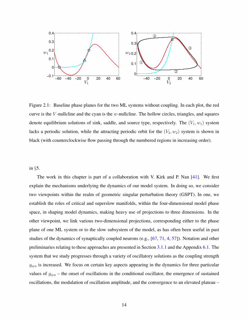
Figure 2.1: Baseline phase planes for the two ML systems without coupling. In each plot, the red
curve is the V -nullcline and the cyan is the w-nullcline. The hollow circles, triangles, and squares
denote equilibrium solutions of sink, saddle, and source type, respectively. The (V1, w1) system
lacks a periodic solution, while the attracting periodic orbit for the (V2, w2) system is shown in
black (with counterclockwise flow passing through the numbered regions in increasing order).
in §5.
The work in this chapter is part of a collaboration with V. Kirk and P. Nan [41]. We first
explain the mechanisms underlying the dynamics of our model system. In doing so, we consider
two viewpoints within the realm of geometric singular perturbation theory (GSPT). In one, we
establish the roles of critical and superslow manifolds, within the four-dimensional model phase
space, in shaping model dynamics, making heavy use of projections to three dimensions. In the
other viewpoint, we link various two-dimensional projections, corresponding either to the phase
plane of one ML system or to the slow subsystem of the model, as has often been useful in past
studies of the dynamics of synaptically coupled neurons (e.g., [67, 71, 4, 57]). Notation and other
preliminaries relating to these approaches are presented in Section 3.1.1 and the Appendix 6.1. The
system that we study progresses through a variety of oscillatory solutions as the coupling strength
gsyn is increased. We focus on certain key aspects appearing in the dynamics for three particular
values of gsyn – the onset of oscillations in the conditional oscillator, the emergence of sustained
oscillations, the modulation of oscillation amplitude, and the convergence to an elevated plateau –
14

such that patterns arising for other gsyn can be readily understood in terms of these components.
The mechanisms underlying these phenomena are analyzed using our two approaches in Section
2.2. Next, in Section 2.3, we revisit the solution types and elucidate which characteristics truly
represent three timescale features. This analysis involves consideration of certain reductions to
two timescales as well as additional analysis of the parameter dependence of solution features in
the three timescale framework. Our results in this area may be useful for characterizing, developing
models of, and analyzing models of experimental data. Finally, Section 2.4 contains a discussion
of our results.
2.1 PRELIMINARIES
Based on simulations of (2.1)-(2.2) over a range of gsyn values, we have selected three fundamental
solution types on which to focus our analysis, specifically those obtained by setting gsyn to 1.0, 4.1
and 5.1. Time series for the attracting solutions at these values of gsyn are shown in Fig. 2.2.
We shall see that the properties of these solutions are indicative of the presence of at least three
timescales.
Our methods for analysis of the model will depend heavily on exploiting the presence of dif-
ferent timescales. As a first step in the analysis, therefore, it is helpful to rescale the variables so
that the important timescales can be explicitly identified. To this end, we define new dimensionless
variables (v1, v2, τ), and voltage and timescales Qv and Qt, respectively, such that
(2.3) V1 = Qv · v1 , V2 = Qv · v2 , t = Qt · τ.
Note that w1 and w2 are already dimensionless in (2.1a-2.1d).
Details of the nondimensionalization procedure, including determination of appropriate values
for Qv and Qt, are given in the Appendix. From this process, we obtain a dimensionless system of
15

0 1000 2000 3000 4000 5000−65
−25
15
55
time (ms)
gsyn= 1.0 (mS/cm2 )
V1 (mV)
V2 (mV)
0 1000 2000 3000 4000 5000−65
−25
15
55
time (ms)
gsyn= 4.1 (mS/cm2 )
0 1000 2000 3000 4000 5000−65
−25
15
55
time (ms)
gsyn= 5.1 (mS/cm2 )
Figure 2.2: Time series for attracting solutions of (2.1)-(2.2) with parameter values as in Table 2.1
and with the indicated values of gsyn.
the form
ε1dv1dτ
= f1(v1, v2, w1)(2.4a)
dw1
dτ= g1(v1, w1)(2.4b)
dv2dτ
= f2(v2, w2)(2.4c)
dw2
dτ= ε2g2(v2, w2) ,(2.4d)
with small parameters ε1, ε2 � 1, where the functions f1, f2, g1 and g2 are specified in (6.3) in the
Appendix. The values of ε1 and ε2 can be varied by changing C1 and φ2, respectively, as shown in
(6.2a); the parameter values given in Table 2.1 yield ε1 = 0.1, ε2 = 0.053.
16

2.1.1 Singular limits: scalings and subsystems
Standard ideas from GSPT [18, 31, 32] are useful in our analysis, although they need to be adapted
to allow for the presence of three timescales in our model. Rewriting the time variable τ as ts, we
see that (2.4) has the form
ε1dv1dts
= f1(v1, v2, w1)(2.5a)
dw1
dts= g1(v1, w1)(2.5b)
dv2dts
= f2(v2, w2)(2.5c)
dw2
dts= ε2g2(v2, w2) ,(2.5d)
where f1, g1, f2, g2 are O(1) functions and ε1, ε2 are small parameters. We refer to changes with
respect to ts as evolution on the slow timescale. Introducing a superslow time tss = ε2ts, which
changes slowly relative to ts, we can derive the rescaled system
ε1ε2dv1dtss
= f1(v1, v2, w1)(2.6a)
ε2dw1
dtss= g1(v1, w1)(2.6b)
ε2dv2dtss
= f2(v2, w2)(2.6c)
dw2
dtss= g2(v2, w2),(2.6d)
which evolves on the superslow timescale. Alternatively, defining a fast time tf = ts/ε1, which
changes quickly relative to ts, we obtain the rescaled system
dv1dtf
= f1(v1, v2, w1)(2.7a)
dw1
dtf= ε1g1(v1, w1)(2.7b)
dv2dtf
= ε1f2(v2, w2)(2.7c)
dw2
dtf= ε1ε2g2(v2, w2),(2.7d)
which evolves on the fast timescale.
17
There are several possible singular limits that can be taken in (2.5)-(2.7), yielding an array of
subsystems. We will use the term reduced problem to refer to a subsystem that is exposed by a limit
that eliminates dynamics faster than the baseline timescale. The phrase layer problem will refer
to a system obtained by eliminating dynamics slower than the baseline. Since a reduced problem
may have more than one timescale, we can define a layer problem for a reduced problem, and we
will refer to the resulting system as a reduced layer problem. These terms will become clearer as
we apply them to specific systems below.
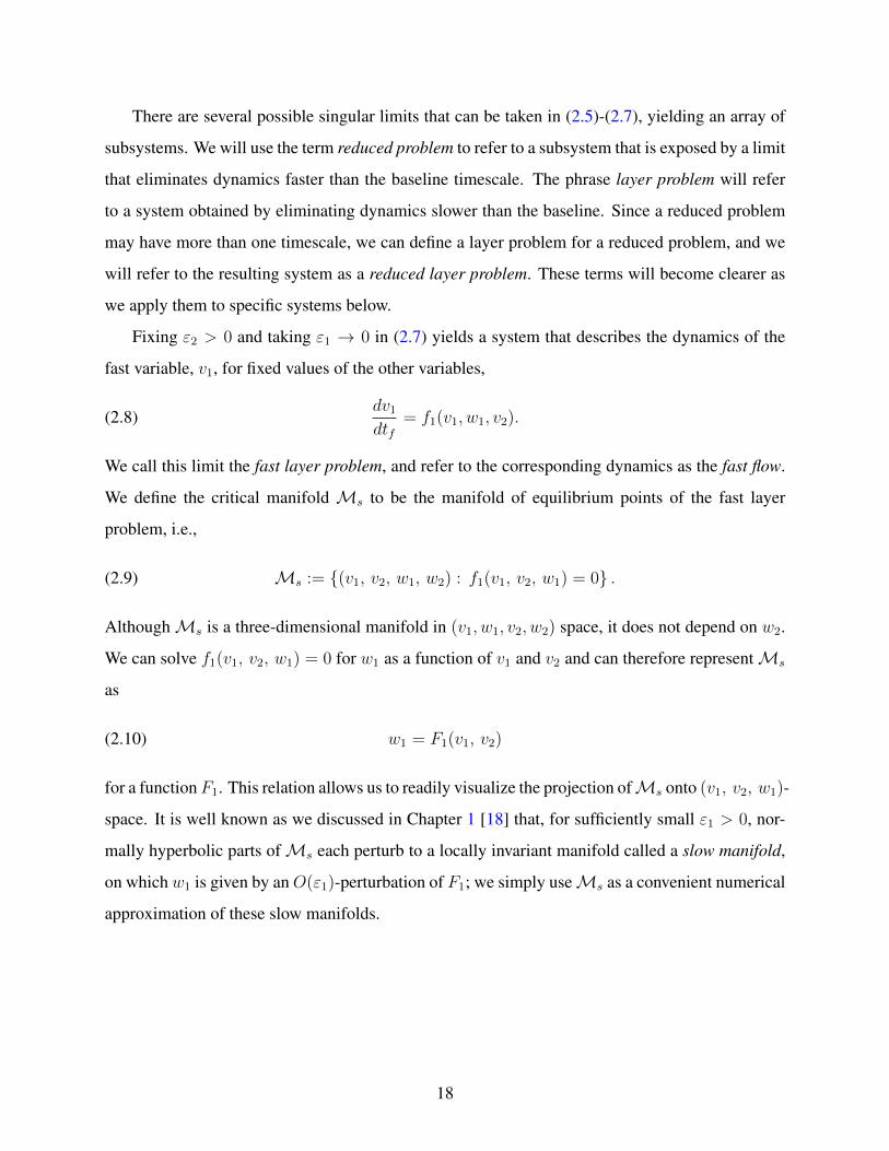
Fixing ε2 > 0 and taking ε1 → 0 in (2.7) yields a system that describes the dynamics of the
fast variable, v1, for fixed values of the other variables,
(2.8)dv1dtf
= f1(v1, w1, v2).
We call this limit the fast layer problem, and refer to the corresponding dynamics as the fast flow.
We define the critical manifold Ms to be the manifold of equilibrium points of the fast layer
problem, i.e.,
(2.9) Ms := {(v1, v2, w1, w2) : f1(v1, v2, w1) = 0} .
AlthoughMs is a three-dimensional manifold in (v1, w1, v2, w2) space, it does not depend on w2.
We can solve f1(v1, v2, w1) = 0 for w1 as a function of v1 and v2 and can therefore representMs
as
(2.10) w1 = F1(v1, v2)
for a functionF1. This relation allows us to readily visualize the projection ofMs onto (v1, v2, w1)-
space. It is well known as we discussed in Chapter 1 [18] that, for sufficiently small ε1 > 0, nor-
mally hyperbolic parts ofMs each perturb to a locally invariant manifold called a slow manifold,
on which w1 is given by anO(ε1)-perturbation of F1; we simply useMs as a convenient numerical
approximation of these slow manifolds.
18

Taking the same limit, i.e., ε1 → 0 with ε2 > 0, in (2.5) yields a system that describes the
dynamics of w1, v2, w2 restricted to the surfaceMs,
dw1
dts= g1(v1, w1) ,(2.11a)
dv2dts
= f2(v2, w2) ,(2.11b)
dw2
dts= ε2g2(v2, w2) ,(2.11c)
subject to the constraint f1(v1, v2, w1) = 0. Since it is obtained by eliminating the fast flow, we
call this system the slow reduced problem. It is itself a multiple timescale problem, since the slow
and superslow timescales are still both present. It is convenient to further separate scales by letting
ε2 → 0 in (2.11); doing so yields the slow reduced layer problem,
dw1
dts= g1(v1, w1) ,(2.12a)
dv2dts
= f2(v2, w2) ,(2.12b)
which describes the dynamics of the slow variables w1 and v2 for fixed values of w2, with all
variables restricted to Ms. Since it takes place entirely on the slow timescale, we refer to the
corresponding dynamics as the slow flow.
Alternatively, fixing ε1 > 0 and taking ε2 → 0 in (2.5) or (2.7) yields the slow layer problem,
which is a different layer problem from (2.12). Starting from (2.5) yields the slow layer problem
in the form
ε1dv1dts
= f1(v1, v2, w1) ,(2.13a)
dw1
dts= g1(v1, w1) ,(2.13b)
dv2dts
= f2(v2, w2) .(2.13c)
System (2.13) still includes two distinct timescales, and we can manipulate the system to obtain
either the fast layer problem (2.8), by rescaling time and taking a limit, or the slow reduced layer
problem (2.12), by taking a limit. We define the superslow manifold,Mss, to be the set of equilib-
rium points of the slow layer problem, i.e.,
(2.14) Mss := {(v1, v2, w1, w2) : f1(v1, v2, w1) = g1(v1, w1) = f2(v2, w2) = 0} .
19

Note thatMss is a subset ofMs. Similarly toMs, the normally hyperbolic parts ofMss perturb
to nearby locally invariant manifolds for ε2 sufficiently small, and we approximate the collection
of these manifolds byMss.
Taking the same limit in (2.6), i.e., ε2 → 0 with ε1 > 0, gives a system that describes the
dynamics of w2 restricted toMss,
(2.15)dw2
dtss= g2(v2, w2) .
We call this system the superslow reduced problem and refer to the corresponding dynamics as the
superslow flow.
There is one more limiting system that turns out to be important for the dynamics we consider.
We define the three-dimensional manifold,Mσ, by
Mσ := {(v1, w1, v2, w2) : f2(v2, w2) = 0}.
Because the dynamics of (v2, w2) decouples from (v1, w1) in (2.4), we can find a function F2 such
that
(2.16) w2 = F2(v2)
onMσ. Differentiation of (2.16) with respect to ts yields
dw2
dts= F ′2(v2)
dv2dts
.
This equation can be combined with (2.5) to obtain the three timescale system
ε1dv1dts
= f1(v1, w1, v2) ,(2.17a)
dw1
dts= g1(v1, w1) ,(2.17b)
dv2dts
=ε2g2(v2, F2(v2))
F ′2(v2)(2.17c)
describing the dynamics onMσ, away from its folds (to leading order in ε2; see Remark 1). An
analogous system was used heavily in the analysis of three timescale dynamics in [35].
20

Remark 1. Just asMs is defined in the singular limit and perturbs to a nearby locally invariant
manifold for 0 < ε1 � 1,Mσ perturbs to a nearby locally invariant manifold for 0 < ε2 � 1.
This manifold is given by w2 = F2(v2) + O(ε2), and additional terms should appear in the v2
equation in (2.17) to reflect this perturbation, but these are higher order in ε2 and we omit them.
It will be useful to work with two systems defined from (2.17). First, taking ε1 → 0 yields the
slow reduced problem for (2.17) governing the dynamics on Ms ∩Mσ. Taking the subsequent
limit ε2 → 0 gives the slow reduced layer problem for (2.17), namely
(2.18)dw1
dts= g1(v1, w1) ,
onMs ∩Mσ; note that this equation is consistent with (2.12) with f2 = 0, although it cannot be
obtained by taking a limit in (2.12) directly.
Second, taking ε2 → 0 directly in (2.17) gives
ε1dv1dts
= f1(v1, w1, v2) ,(2.19a)
dw1
dts= g1(v1, w1) .(2.19b)
System (2.19) is the slow layer problem for (2.17). To distinguish it from (2.13), we will also call
(2.19) the v2-frozen system, with solutions that we call v2-frozen solutions. Similarly, when it is
helpful, we will refer to (2.18) as the v2-frozen system reduced problem and (2.8) as the v2-frozen
system layer problem, since these can be obtained through appropriate limits from (2.19).
For reference, we summarize the subsystems that are useful for describing the dynamics of
(2.4) in Table 2.2.
Within the context of GSPT, the usual way to proceed from here is to construct singular pe-
riodic orbits by concatenating solution segments of singular limit systems (see Figure 1.1 in the
introduction section). A similar method could also be used to explain the oscillations seen in three
timescale systems, although the process would be more complicated since there are more than two
singular limit systems to be considered. In this chapter, for reasons of brevity, we choose not to
show detailed constructions of singular orbits and subsequent analysis of how these perturb. In-
stead, we appeal to intuition based on the way the technique works in two timescale systems to
explain the mechanisms underlying solutions generated in simulations done with a separation of
21
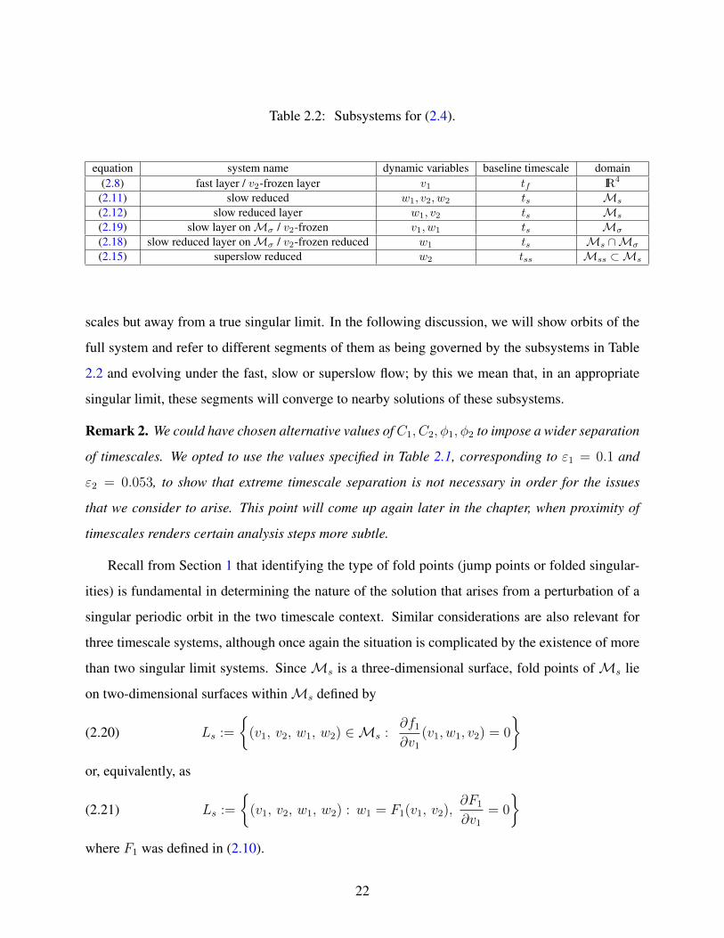
Table 2.2: Subsystems for (2.4).
equation system name dynamic variables baseline timescale domain(2.8) fast layer / v2-frozen layer v1 tf IR4
(2.11) slow reduced w1, v2, w2 ts Ms
(2.12) slow reduced layer w1, v2 ts Ms
(2.19) slow layer onMσ / v2-frozen v1, w1 ts Mσ
(2.18) slow reduced layer onMσ / v2-frozen reduced w1 ts Ms ∩Mσ
(2.15) superslow reduced w2 tss Mss ⊂Ms
scales but away from a true singular limit. In the following discussion, we will show orbits of the
full system and refer to different segments of them as being governed by the subsystems in Table
2.2 and evolving under the fast, slow or superslow flow; by this we mean that, in an appropriate
singular limit, these segments will converge to nearby solutions of these subsystems.
Remark 2. We could have chosen alternative values ofC1, C2, φ1, φ2 to impose a wider separation
of timescales. We opted to use the values specified in Table 2.1, corresponding to ε1 = 0.1 and
ε2 = 0.053, to show that extreme timescale separation is not necessary in order for the issues
that we consider to arise. This point will come up again later in the chapter, when proximity of
timescales renders certain analysis steps more subtle.
Recall from Section 1 that identifying the type of fold points (jump points or folded singular-
ities) is fundamental in determining the nature of the solution that arises from a perturbation of a
singular periodic orbit in the two timescale context. Similar considerations are also relevant for
three timescale systems, although once again the situation is complicated by the existence of more
than two singular limit systems. SinceMs is a three-dimensional surface, fold points ofMs lie
on two-dimensional surfaces withinMs defined by
(2.20) Ls :=
{(v1, v2, w1, w2) ∈Ms :
∂f1∂v1
(v1, w1, v2) = 0
}or, equivalently, as
(2.21) Ls :=
{(v1, v2, w1, w2) : w1 = F1(v1, v2),
∂F1
∂v1= 0
}where F1 was defined in (2.10).
22
Folded singularities for three timescale systems have not been comprehensively studied, al-
though [35] classifies the folded singularities in a particular three dimensional, three timescale
system by extending ideas from two timescale systems, and [81] extends the concepts developed
for two timescale systems with two slow variables to systems with three or more slow variables;
ideas related to both of these approaches appear in [77], where a degenerate type of folded singu-
larity that arises naturally in three timescale systems is identified and some analysis of the related
dynamics is given.
In the usual manner, we define the desingularised slow reduced problem by differentiating
the algebraic equation defining Ms (i.e., f1(v1, v2, w1) = 0) and rescaling time using τs =
(∂F1/∂v1)ts, yielding
dv1dτs
= g1(v1, w1)−∂F1
∂v2f2(v2, w2) ,(2.22a)
dv2dτs
=∂F1
∂v1f2(v2, w2) ,(2.22b)
dw2
dτs= ε2
∂F1
∂v1g2(v2, w2) .(2.22c)
We then look for equilibria of (2.22) that are not equilibria of the full system; these are what we
refer to as folded singularities ofMs. We find that they lie on one-dimensional curves within Ls
defined by
(2.23) FS :=
{(v1, v2, w1, w2) ∈ Ls : g1(v1, w1)−
∂F1
∂v2(v1, v2)f2(v2, w2) = 0
}.
Away from Mss, the linearisation of (2.22) at a folded singularity has one zero eigenvalue (due
to there being a curve of folded singularities, as in [81]) and two other eigenvalues; the folded
singularities can be classified using these other eigenvalues, as in [35, 81]. As we will see, the
location and type of folded singularities withinMs depends on gsyn. We note that points where
Mss and Ls intersect are always folded singularities since g1 = f2 = 0 onMss; some discussion
of this degenerate type of folded singularity is contained in [77].
Since Mss is a one-dimensional subset of Ms, fold points of Mss occur at isolated points;
these are located on the set
(2.24) Lss :=
{(v1, v2, w1, w2) ∈Mss :
∂f2∂v2
(v2, w2) = 0 or∂f1∂v1
∂g1∂w1
− ∂f1∂w1
∂g1∂v1
= 0
}.
23

For all values of gsyn that we consider below, points that satisfy the latter condition lie on the
middle sheet of Ms and hence will not play a role in the dynamics, and points that satisfy the
former condition are jump points.
2.1.2 Effect of coupling
When gsyn = 0, our model decouples into two systems, each of which has two variables and a
two timescale structure. For the parameter values we have chosen, the nullclines for the uncoupled
systems are qualitatively as shown in Figure 2.1. Each v nullcline is cubic shaped, with outer
branches that are attracting relative to the v dynamics and a repelling inner branch. When solutions
are near the outer branch with lower (resp. higher) v values, we say that the system is in the silent
(resp. active) phase.
Since the coupling in our system is unidirectional, the oscillations in (v2, w2) are independent
of the value of gsyn and of the dynamics of v1 and w1; they are standard relaxation oscillations
consisting of a superslow excursion through the silent phase (Fig. 2.1B, 1©), a slow jump away
from the v2 nullcline up to the active phase (Fig. 2.1B, 2©), a superslow excursion through the
active phase (Fig. 2.1B, 3©), and a slow jump back to the silent phase (Fig. 2.1B, 4©). By contrast,
v1 and w1 depend on gsyn and, if gsyn > 0, on v2 and w2. For positive gsyn we find it helpful to
consider the phase plane for the v2-frozen system (2.19) for various fixed values of v2; this is a
reasonable approach to take when v2 is in a superslow phase, i.e., if the dynamics is close toMσ.
Figure 2.3 shows configurations of the v1 and w1 nullclines for (2.19) for several different values
of v2 with gsyn = 5.1. Note that the v1 nullcline satisfies (2.10) and is in fact a section ofMs.
Continuing in this spirit, bifurcation diagrams can be obtained for (2.19) using v2 as the bifur-
cation parameter. Examples are shown in Figure 2.4 for several values of gsyn. For gsyn = 4.1 and
gsyn = 5.1, several families of periodic orbits are seen. The first is almost invisible on the scale of
Figure 2.4; as v2 is increased a branch of unstable small amplitude periodic orbits is created in a
homoclinic bifurcation involving the middle branch of equilibria and is destroyed in a subcritical
AH bifurcation of the lower branch of equilibria. A second family of stable periodic orbits of much
larger amplitude is created in a homoclinic bifurcation also involving the middle branch of equi-
libria. For gsyn = 5.1, but not 4.1, this family of orbits terminates for larger v2 when it coalesces
24

−0.4 −0.2 0 0.2 0.4 0.6−0.1
0
0.1
0.2
0.3
0.4
v1
w1
−0.4 −0.2 0 0.2 0.4 0.6−0.1
0
0.1
0.2
0.3
0.4
v1
w1
−0.4 −0.2 0 0.2 0.4 0.6−0.1
0
0.1
0.2
0.3
0.4
v1
w1
Figure 2.3: Nullclines for v1 (red) and w1 (cyan) for the v2-frozen system (2.19). The red curve
is a slice throughMs taken at a fixed v2 and restricted to the (v1, w1) plane. The cyan curve is the
restriction of the w1 nullcline to the (v1, w1) plane. Varying v2 changes the red curve but not the
cyan curve. From left to right: v2=-0.7,-0.4,0.2, all with gsyn = 5.1. Circles, triangles, and squares
denote equilibria of (2.19) of sink, saddle, and source type, resp.
−0.5 −0.4 −0.3 −0.2 −0.1 0 0.1
−0.5
0
0.5
v2
v1
−0.5 −0.4 −0.3 −0.2 −0.1 0 0.1
−0.5
0
0.5
v2
v1
−0.5 −0.4 −0.3 −0.2 −0.1 0 0.1
−0.5
0
0.5
v2
v1
Figure 2.4: Bifurcation diagrams for (2.19) with v2 as a parameter. From left to right, gsyn =
1.0, 4.1, 5.1. Solid (resp. dashed) red curves indicate stable (resp. unstable) equilibria, and black
curves indicate periodic solutions (stability not indicated).
with a third family of unstable periodic solutions born in a subcritical AH bifurcation at relatively
large v2. For gsyn = 4.1, even with the coupling function S(v2) set to its upper limit of 1, the upper
equilibrium point of (2.19) remains unstable and the stable periodic orbits persist as v2 →∞.
Allowing both gsyn and v2 to vary, we find bifurcation curves in the (v2, gsyn) parameter plane,
as illustrated in Figure 2.5. The green (resp. blue) curve in the left panel is the curve of AH
bifurcations on the lower (resp. upper) branch of equilibria. These approach horizontal asymptotes
25

−0.4 −0.2 0 0.2
1
2
3
4
5
6
7
v2
gsyn
−0.428 −0.424 −0.42
4.2
4.3
4.4
4.5
v2
gsyn
Figure 2.5: Bifurcation curves for (2.19) in (v2, gsyn) parameter space. Left: Two curves of AH
bifurcations (green, lower v1; blue, higher v1) and their horizontal asymptotes (dashed). Right:
Enlargement of part of left panel showing, in order of increasing v2 and gsyn, part of the lower AH
curve (green), two overlapping homoclinic bifurcation curves (red), and, for comparison, the curve
of saddle-node bifurcations that occurs at relatively low v1 (black).
as v2 increases; the lower asymptote is at gsyn ≈ 1.0319 =: g while the upper asymptote is at
gsyn ≈ 4.2628 =: g. Existence of the upper asymptote implies that the (v1, w1) system will not
oscillate for any fixed gsyn > g if v2 is fixed at a large enough value; this is illustrated in the right
panel of Figure 2.4. The onset of stable oscillations, on the other hand, is not directly tied to the
green AH curve, since that curve relates to the family of unstable oscillations near the lower branch
of equilibria. To identify the onset of stable oscillations, we compute the curve of homoclinic
bifurcations through which the stable large amplitude oscillations arise as v2 increases. It turns out
that this curve lies extremely close to the lower AH curve (compare the red and green curves in the
right panel of Figure 2.5), with approximately the same asymptote. Thus, for gsyn < g, there is no
value at which v2 can be fixed to yield oscillations in (v1, w1), while for gsyn ∈ (g, g), oscillations
occur for all v2 above the homoclinic bifurcation.
The structure of the bifurcation set in Figure 2.5 stems in part from the form of the coupling
function S(v2) in (2.1), as defined in (2.2) and shown in Figure 2.6. For v2 sufficiently small or
sufficiently large, S(v2) varies little in response to changes in v2, whereas for intermediate values
26
−0.6 −0.2 0.2
0
0.2
0.4
0.6
0.8
v2
w2, S
Figure 2.6: Graph of S(v2) (blue) and locus of the v2-nullcline (black/red). The red section of the
v2-nullcline indicates the range of v2 values over which S(v2) is steeply sloped.
of v2, S(v2) changes rapidly with v2 (red in Figure 2.6). As a consequence, changes of v2 within
the intermediate interval result in significant effects on the v1 equation, while changes in v2 outside
of this domain have little effect. This saturation of S explains why the horizontal asymptotes in
Figure 2.5 exist and why certain bifurcations cannot be achieved by increasing v2 in (2.19) if gsyn
is not sufficiently large. Figure 2.6 also shows where the steepest part of S lies relative to the v2
nullcline. We see that S(v2) is sensitive to changes in v2 over the silent phase and over jumps
between phases but is insensitive to v2 in the active phase for the parameter values we use.
As noted above, the (v2, w2) dynamics is not dependent on (v1, w1) or on gsyn; with parame-
ters fixed as in Table 2.1, the (v2, w2) variables trace out a relaxation oscillation, shown in the right
panel of Figure 2.1. It will be helpful to define some reference points along the relaxation oscil-
lation. Figure 2.7 shows the (v2, w2) oscillation from Figure 2.1 plotted in non-dimensionalised
coordinates, with green symbols marking points at the transition between the four different sec-
tions of the oscillation. These symbols have the same interpretation in all the figures and analysis
that follow.
27

−0.5 −0.3 −0.1 0.1 0.3 0.5
0
0.1
0.2
0.3
0.4
1©
2©
3©
4©
v2
w2
Figure 2.7: Attracting dynamics in (v2, w2)-space. The green symbols mark the approximate
points of transition between the slow and superslow sections of the oscillation: the square and star
mark the transitions from slow to superslow motion, and the circle and triangle mark the transitions
from superslow to slow motion. The circled numbers label the sections of the oscillation, using the
same convention as in the right panel of Figure 2.1.
2.2 ANALYSIS OF THREE TIMESCALE SOLUTIONS
Simulation of (2.4) over a range of parameter values yields a variety of solution behaviors, with
variation in gsyn giving a particularly nice progression of features. We focus our analysis on three
values of gsyn; these values highlight the distinct combinations of dynamic mechanisms that can
arise for (2.4) and together capture the most interesting dynamic effects that we have identified
over a range of gsyn values. The case gsyn = 1.0 represents an interesting transitional case between
solutions in which v1 remains relatively steady at a low level and solutions for which v1 spikes
repeatedly. The cases gsyn = 4.1 and gsyn = 5.1 are representative of two related yet distinct
solution behaviors each seen over a wide range of gsyn values.
In the following, we will present analysis from two points of view, one that focuses on the
roles ofMs andMss in organizing the flow of the full model and another that focuses on how the
oscillations of (v2, w2) affect the dynamics of (v1, w1). The inclusion of both perspectives, we feel,
provides the clearest picture of how the dynamics emerges, and may be of use to those readers who
28

typically adopt only one perspective or the other.
2.2.1 Case 1: gsyn=1.0
2.2.1.1 (v1, w1) driven by (v2, w2) We now consider (2.1) from the perspective of a fast-slow
system driven by a slow-superslow oscillation. The use of this kind of perspective has proved
helpful in past analyses of various models with two timescales (e.g., [71, 70, 57, 55, 12]).
Recall that for the parameter values we are considering, in the absence of coupling, the (v1, w1)
system has a stable equilibrium but no oscillatory solution. If coupling is introduced by setting
gsyn = 1.0, however, then oscillations in v1 are observed, as can be seen in Figure 2.2. It might
be natural to ascribe the onset of these oscillations to variation of v2 pushing the v2-frozen system
(2.19) through a bifurcation at which oscillations are born. As shown in Figures 2.4 and 2.5, how-
ever, there is no such bifurcation for gsyn = 1.0. The key point in considering the dynamics with
gsyn = 1.0 from the perspective of (v2, w2) driving (v1, w1) is to explain the observed oscillations
in v1.
To provide this explanation, we consider the phases of the (v2, w2) oscillation in succession.
The yellow dot in Figure 2.9 marks the point in phase 3© where the conditions f1 = g1 = f2 = 0
become (approximately) satisfied; the trajectory at this point lies on the v2-nullcline when projected
to the (v2, w2) plane and at the intersection of the v1 and w1 nullclines of the v2-frozen system
(2.19) when projected to the (v1, w1) plane. From the yellow dot, the solution evolves under the
superslow reduced problem (2.15) with v2 slaved to w2. The evolution of v2 in turn moves the v1
nullcline of (2.19) on the superslow timescale, while the w1 nullcline is independent of v2 and thus
remains fixed. The (v1, w1) projection of the trajectory then tracks the intersection of the v1 and
w1 nullclines. In fact, v2 > 0 throughout phase 3©, so based on the shape of S(v2), which provides
the coupling from v2 to v1, these intersection points depend only very weakly on v2 (see Figure
2.6). Thus, if projected to the (v1, w1) plane, the yellow dot would lie almost on the green triangle
that marks the end of phase 3©, and the trajectory remains near the green triangle throughout this
part of phase 3© (Figure 2.8).
After the trajectory passes the green triangle and moves into phase 4©, the condition f2 = 0 no
longer applies. The flow is now governed by the slow reduced layer problem (2.12). The trajectory
29

−0.5 0 0.5
0
0.1
0.2
0.3
v1
w1
−0.5 −0.3 −0.1
0
0.02
0.04
1© 2©4©
v1
w1
Figure 2.8: An attracting solution of (2.4) for gsyn = 1.0 (black curve) projected to the (v1, w1)
plane; the right panel shows an enlargement of part of the left panel. Circled numbers and green
symbols correspond to phases of the (v2, w2) oscillation and the transition points, as shown in
Figure 2.7. The cyan curve is the w1 nullcline for (2.19), which is independent of v2, while the red
curves are the v1 nullclines for (2.19) for v2 = v2max (higher red curve) and v2 = v2min(lower red
curve).
still lies onMs, and thus, in the projection to the (v1, w1) plane, is on the curve f1(v1, w1, v2) = 0,
but it diverges from the w1-nullcline (cyan curve in Figure 2.8). Correspondingly, the trajectory
diverges from the red curve in Figure 2.9, which shows the w1-coordinate of the intersection of v1-
and w1-nullclines of (2.19) for each v2.
Phase 4© ends when the trajectory converges to a critical point of (2.12), at which time its
projection to the (v2, w2) plane reaches the left branch of the v2-nullcline. The v2-coordinate of
this point is the minimal value of v2 along the trajectory; call it v2min. Within the (v1, w1) plane,
the trajectory is seen to converge to a point at the intersection of the v1 and w1 nullclines for the
v2-frozen system (2.19), with the v1 nullcline computed with v2 = v2min(green star in Figure
2.8). This convergence corresponds to the end of the jump between branches ofMss withinMls
described in the previous subsection.
Next, phase 1© is governed by the superslow reduced flow (2.15), as for phase 3©. Under this
flow, the v1-nullcline for (2.19) moves superslowly in the (v1, w1) plane while the w1-nullcline
30
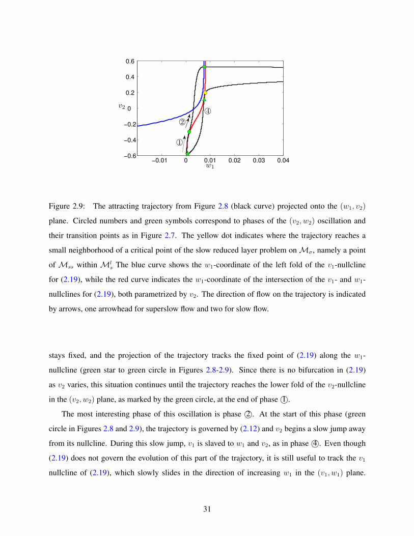
−0.01 0 0.01 0.02 0.03 0.04−0.6
−0.4
−0.2
0
0.2
0.4
0.6
1©
2©4©
w1
v2
Figure 2.9: The attracting trajectory from Figure 2.8 (black curve) projected onto the (w1, v2)
plane. Circled numbers and green symbols correspond to phases of the (v2, w2) oscillation and
their transition points as in Figure 2.7. The yellow dot indicates where the trajectory reaches a
small neighborhood of a critical point of the slow reduced layer problem onMσ, namely a point
of Mss within Mls The blue curve shows the w1-coordinate of the left fold of the v1-nullcline
for (2.19), while the red curve indicates the w1-coordinate of the intersection of the v1- and w1-
nullclines for (2.19), both parametrized by v2. The direction of flow on the trajectory is indicated
by arrows, one arrowhead for superslow flow and two for slow flow.
stays fixed, and the projection of the trajectory tracks the fixed point of (2.19) along the w1-
nullcline (green star to green circle in Figures 2.8-2.9). Since there is no bifurcation in (2.19)
as v2 varies, this situation continues until the trajectory reaches the lower fold of the v2-nullcline
in the (v2, w2) plane, as marked by the green circle, at the end of phase 1©.
The most interesting phase of this oscillation is phase 2©. At the start of this phase (green
circle in Figures 2.8 and 2.9), the trajectory is governed by (2.12) and v2 begins a slow jump away
from its nullcline. During this slow jump, v1 is slaved to w1 and v2, as in phase 4©. Even though
(2.19) does not govern the evolution of this part of the trajectory, it is still useful to track the v1
nullcline of (2.19), which slowly slides in the direction of increasing w1 in the (v1, w1) plane.
31

Each such nullcline has two folds; as can be seen in Figure 2.9, the slow flow of (2.12) steers
the trajectory across the one-dimensional curve of lower folds of the family of v1 nullclines (blue
curve), projected to the (w1, v2) space. Thus, we observe that the flow of (2.12), in which the two
slow variables conspire to pull the trajectory away from the curve of fixed points of (2.19) and
across the curve of lower folds of the family of v1-nullclines, is crucial for the emergence of an
oscillation in v1 for gsyn = 1.0.
Following the fold crossing, there is a fast jump in v1 governed by (2.8), from left to right
branches of the v1-nullcline family in the projection to the (v1, w1) plane. If we had a greater
separation of timescales, then the jump would occur almost as soon as the fold was crossed. With
the weaker separation that we consider, the jump is delayed; it begins quite close to the end of phase
2© and ends during phase 3© (Figure 2.8, right panel). Once the jump in v1 is complete, just after
the start of phase 3©, the trajectory evolves under (2.18) or, equivalently, under the reduced problem
for (2.19), tracking the right branches of the v1-nullclines in the direction of increasing w1 in the
projection to the (v1, w1) plane (Figure 2.8, left and Figure 2.9). The trajectory eventually reaches
the right knee curve of the v1-nullcline family and jumps down to the left v1-nullcline branches
under (2.8) or, equivalently, under the layer problem of (2.19). Finally, the trajectory converges
under (2.18) to the curve of critical points where the v1-nullclines intersect thew1-nullcline (yellow
dot in Figure 2.9), bringing us back to where we started our description.
Remark 3. In the true singular limit, we expect that the fast jump up of v1 would happen instantly
with respect to the slow timescale, during phase 2©. After that jump, w1 and v2 would evolve
according to (2.12), continuing phase 2©, until being interrupted again by the fast jump down of v1.
Finally, the slow evolution of (2.12) would continue until convergence to where f1 = g1 = f2 = 0,
analogous to our yellow dot point, at the end of phase 2©. This progression is expected from GSPT
and we have observed it numerically (not shown).
2.2.2 Case 2: gsyn=4.1
2.2.2.1 (v1, w1) driven by (v2, w2) We now use our alternative perspective to explain proper-
ties of the attracting solution when gsyn = 4.1. Figure 2.4 shows that treating v2 as a parameter
in the v2-frozen system (2.19) and increasing v2 from its minimal relevant value pushes (2.19)
32

through a homoclinic bifurcation, resulting in the appearance of oscillatory solutions of (2.19);
these oscillations persist no matter how large v2 becomes, which explains why the v1 spikes con-
tinue throughout phase 3© as v2 drifts on the superslow timescale and only end after v2 drops below
the homoclinic bifurcation value during phase 4©.
Next, we explain why the amplitude of the v1 spikes decreases progressively during phase
1© until v2 jumps up in phase 2©, and then remains approximately constant throughout phase
3©. Consider the effect of v2 on the position of the v1-nullcline of (2.19). At the start of phase
1© the v1- and w1-nullclines intersect in three critical points (Figure 2.10, lowest red curve and
cyan curve). Under (2.17), as v2 increases on the superslow timescale during phase 1©, it raises
the corresponding v1-nullcline of (2.19). This rise is not uniform in v1, however; since it occurs
through the term gsynS(v2)(v1−Vsyn) in (2.1), a fixed change in v2 causes a relatively large change
in the w1-values along the part of the v1-nullcline with v1 far below Vsyn, including the left branch
of the v1-nullcline, and a relatively small change where |v1 − Vsyn| is small, including the right
branch of the v1-nullcline (Figure 2.10).
The increase in v2 causes a bifurcation in which two of (v1, w1) critical points near the left
knee of the v1-nullcline, with v1 values far from Vsyn, merge and annihilate. For each v2 above the
bifurcation value, (2.19) exhibits a stable relaxation oscillation involving fast jumps in v1 between
branches of the v1-nullcline alternating with slow drift in (v1, w1) along these branches. Since the
right branch of the nullcline depends little on v2, each jump down occurs from a similar value of
w1 even as v2 varies (Figure 2.10). The minimal values of v1 within spikes are determined by the
fast flow and increase with v2, since they are on the left branches of the v1-nullclines. Thus, we
find increasing v1 values along successive v1 spike troughs before v2 becomes active. Furthermore,
the jumps up in v1 occur from larger w1 values across successive spikes as v2 increases. These
jumps land at points on similar negatively sloped right branches, meaning that an increase in w1
translates to a decrease in v1 at the landing point (Figure 2.10). Thus, peak values of v1 decrease
across successive spikes during this phase.
When phase 1© ends, v2 jumps up through and beyond the active range of S(v2) (Figure 2.6) to
the right branch of its nullcline in the (v2, w2) phase plane, where phase 3© begins. The (v1, w1) re-
laxation oscillations continue; since S(v2) remains approximately constant, so does the v1-nullcline
and hence so do the quantitative features of the relaxation oscillation. The insensitivity of the v1
33

−0.4 −0.2 0 0.2 0.4 0.6−0.1
0
0.1
0.2
0.3
0.4
v1
w1
Figure 2.10: An attracting solution of (2.4) for gsyn = 4.1, projected to (v1, w1)-space (black
curve). The red curves are v1-nullclines for a selection of fixed values of v2; these move upwards
as v2 increases. The cyan curve is the w1-nullcline, which is independent of v2, and the blue curve
denotes the left folds of the v1-nullclines over the full range of v2 arising during v2 oscillations.
equation to v2 in phase 3© explains why the v1 spikes have approximately constant amplitude
throughout this phase (upper right cycles in the trajectory in Figure 2.10).
The discussion above shows how variations in v2 can shape the v1 spikes: superslow drift in
v2 imposes a superslow v1 spike amplitude modulation. To appreciate fully how transitions in the
v2 dynamics relate to the (v1, w1) dynamics, we consider the projection of the attracting solution
onto the (w1, v2) plane (see Figure 2.11), During the part of phase 1© when there is no spiking,
the trajectory evolves under (2.15), moving along an attracting branch of Mss (near the single
arrow). A fast excursion away from Mss, and in fact away from Ms altogether, occurs when
the branch ofMss crosses the fold ofMs (green diamond). At the onset of the fast jump, v2 is
still below the value corresponding to the left fold of the v2-nullcline and continues to drift on
the superslow timescale while the (v1, w1) system has alternating fast and slow segments, with w1
oscillating between the folds of the v1-nullcline (blue curves), under (2.17). Once the lower fold of
the v2-nullcline is crossed (green circle), (2.12) governs the slow segments of the trajectory; these
34

0 0.1 0.2 0.3 0.4−0.6
−0.4
−0.2
0
0.2
0.4
0.6
w1
v2
1©
2©
3©
4©
Figure 2.11: Projection to the (w1, v2)-plane illuminates several features of the periodic solution
(black) for gsyn = 4.1. The red curves are branches of Mss or, equivalently, critical points of
(2.19), the blue curves are the left (smaller w1) and right (larger w1) folds of the v1-nullcline, the
green diamond marks the time point when v1 begins spiking, and the other green symbols have the
same meanings as in Figure 2.7.
alternate with fast jumps governed by (2.8), but there is only time for a few of these jumps, since
w1 and v2 evolve on the same timescale during this phase. The return of (v2, w2) to a neighborhood
of the v2-nullcline occurs as v2 reaches its maximum value (green square); then the evolution of
v2 becomes superslow again, so that only small decreases in v2 are seen during the subsequent
spikes governed by (2.19). This progression continues until (v2, w2) crosses the right fold of the
v2-nullcline (green triangle), at which time another slow jump in v2 occurs. Under (2.12), the
trajectory then converges back toMss, completing the cycle.
Figure 2.11 shows clearly the v2-dependence of thew1 coordinate on folds of the v1-nullcline of
(2.19), as discussed earlier. The w1 coordinate of the left folds of the v1-nullcline depends strongly
on v2 while v2 is negative but becomes approximately independent of v2 at positive v2, while the
w1 coordinate of the right folds is more weakly dependent on v2 and also becomes approximately
independent of v2 for v2 sufficiently large (Figure 2.11). Correspondingly, the minimal w1 value
35

−0.4 −0.2 0 0.2 0.4 0.6−0.1
0
0.1
0.2
0.3
0.4
w1
v1
Figure 2.12: An attracting solution of (2.4) for gsyn = 5.1, projected to (v1, w1)-space (black
curve), together with nullclines for (2.19). Colours of curves are as in Figure 2.10.
during a spike increases on subsequent spikes when the (v2, w2) system is in phase 1©, as does
the minimal v1 value, and is approximately constant when the (v2, w2) system is in phase 3©. The
maximal w1 value remains relatively constant over all spikes.
2.2.3 Case 3: gsyn=5.1
2.2.3.1 (v1, w1) driven by (v2, w2) Comparing the relevant bifurcation diagrams in Figure 2.4
shows that changes in v2 have a qualitatively similar impact on the v2-frozen system (2.19) for
gsyn = 5.1 as for gsyn = 4.1 except that for gsyn = 5.1, when v2 becomes sufficiently large, oscil-
lations of (2.19) are lost as a stable critical point at elevated v1 is born through an AH bifurcation.
Correspondingly, comparing Figures 2.12 and 2.10 reveals a similar progression of v1-nullclines
except that when gsyn = 5.1, the upper knee of the v1-nullcline eventually crosses the w1-nullcline,
so that the w1-nullcline intersects the uppermost v1-nullcline on its right branch. The trajectory
tends towards this intersection point on the slow timescale during phase 2© and remains in a small
neighborhood of the point throughout phase 3©.
Similarly, there is a strong resemblance between the slow phase plane projections in Figures
36

0 0.1 0.2 0.3 0.4
−0.6
−0.4
−0.2
0
0.2
0.4
0.6
w1
v2 4©
3©
2©
1©
0.31 0.33 0.35 0.37
−0.2
0
0.2
0.4
0.6
w1
v2
Figure 2.13: Projection to the (w1, v2) plane illuminates several features of the periodic solution
(black) for gsyn = 5.1. Color coding and symbols have the same meaning as in Figure 2.11, except
there is now a diamond appearing on the upper (larger w1) branch ofMss, corresponding to the
location of an AH bifurcation in the frozen system (2.19) with v2 treated as a parameter. Right
panel shows an enlarged view.
2.13 and 2.11. The key new feature that arises for gsyn = 5.1 is that there is an attracting limit
point of (2.12) at the green square in Figure 2.13. This point becomes attracting because the curve
of critical points of (2.19) (red) crosses through the fold curve (blue) with increasing v2; due to the
projection, the crossing appears as a tangency in Figure 2.13 (green diamond). After the trajectory
reaches the green square, it drifts back down the red curve on the superslow timescale under (2.15)
until it returns to the fold line (green square to green triangle) and then departs from the nullcline
intersection curve on the slow timescale, again under (2.15), converging towards the lower stable
branch ofMss.
Importantly, as noted in the previous subsection, the convergence to the limit point on the upper
branch ofMss occurs on the slow timescale, governed by (2.12). That is, while v2 evolves along
the left branch of the v2-nullcline on the superslow timescale as part of (2.17), (v1, w1) engage in
fast-slow relaxation oscillations as described by their equations, which comprise (2.19). Once v2
reaches the lower fold of the v2-nullcline, however, there is a transition to a phase of slow flow of
(2.12) with v1 ≈ v1(w1, v2) satisfying f1(v1(w1, v2), v2, w1) = 0. The linearization of (2.12) about
37

its limit point on Mss yields an upper triangular matrix with real eigenvalues, which can easily
be shown to be negative as expected. Thus, this convergence features a direct transition from v1
spikes to a v1 plateau, with no damped oscillations. We shall see later that this property contrasts
with features of similar solutions in two timescale systems.
2.3 IDENTIFYING THREE TIMESCALE FEATURES
We next seek to identify which aspects of the solutions discussed above are truly three timescale
features in some reasonable sense. In this section we find it useful to work with our original
dimensional system (2.1), which produces the solutions shown in Figure 2.2, but, for convenience,
we omit units on the parameter values.
Our approach is to transform (2.1) into certain two timescale systems by adjusting system
parameters, then consider whether these systems can generate solutions that are similar to the three
cases considered in Section 2.2. We will exaggerate the timescale separation in the three timescale
system, speeding up V1 by decreasing C1 from 8 to 0.8 and slowing down w2 by decreasing φ2
from 0.001 to 0.0001. This amounts to reducing both ε1 and ε2 by a factor of 10, to 0.01 and
0.0053, respectively. In our original scaling and in this exaggerated version, our system has 1 fast,
2 slow, and 1 superslow (1F, 2S, 1SS) variables. There are many ways to regroup timescales to
transform this system into a two timescale system. One natural approach is to slow down V1, say
by setting C1 = 80, so that it evolves on the same timescale as w1 and V2, resulting in a 3 slow, 1
superslow (3S, 1SS) system; similar effects are seen if w1, V2 and w2 are sped up appropriately to
produce a system with three fast and one slow (3F, 1S) variables. Another approach is to speed up
w2, say by increasing φ2 to 0.01, so that it evolves on the same slow timescale as V2 and w1 and we
have a 1 fast, 3 slow (1F, 3S) system; qualitatively similar effects will be seen for a one slow, three
superslow (1S, 3SS) system obtained by slowing V1, w1 and V2 appropriately. Other rescalings are
also possible, leading to pairs of variables on each of two scales, but these require more significant
changes, namely modifying the relative speeds of evolution of two variables or altering the speed
of one variable by two orders of magnitude, and so will not be considered.
38

Figure 2.14: Projections of solutions for gsyn = 1.0 onto (V1, V2, w2)-space. The solution tra-
jectory (black curve) exhibits a spike in V1 for the (1F, 2S, 1SS) system (left) but not for the (3S,
1SS) system (right). In both cases, the red curves areMss, with stable (unstable) branches drawn
as solid (dashed) curves. For the (1F, 2S, 1SS) case, the blue surface represents the lower fold of
Ms. The same surface is shown in the (3S, 1SS) case for comparison, althoughMs is no longer
meaningful.
2.3.1 gsyn = 1.0: recruitment of a transient V1 spike
When gsyn = 1.0, (2.1) generates a solution with a single V1 spike per period, as shown in the first
panel of Figure 2.2. With exaggerated timescale separation, there is little change in this solution.
We first compare this solution to solutions from the (3S,1SS) version of the (2.1) described above.
Projections onto (V1, V2, w2)-space show that in the (1F, 2S, 1SS) system, the trajectory reaches
the lower fold surface ofMs and jumps to higher V1. No analogous jump occurs in the (3S, 1SS)
case with gsyn = 1.0 (Figure 2.14), resulting in an absence of spikes in the V1 time course (Figure
2.15, top panel). The fact that (2.19) does not have an AH bifurcation when the frozen variable
v2 is varied can be used to explain why there is no V1 spike in the (3S, 1SS) case. Consider a
trajectory of the (3S, 1SS) system evolving under the superslow flow on the critical manifold for
that system, namelyMss, on a branch where V1 and V2 are low. Suppose this trajectory reaches a
fold ofMss such that a transition to the slow layer problem occurs. By construction, the slow layer
39
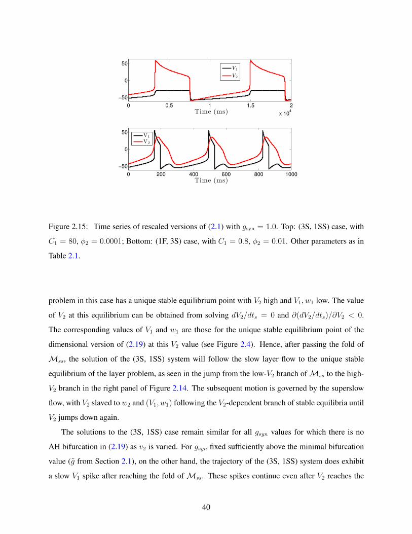
0 0.5 1 1.5 2
x 104
−50
0
50
Time (ms)
V1
V2
0 200 400 600 800 1000
−50
0
50
Time (ms)
V1
V2
Figure 2.15: Time series of rescaled versions of (2.1) with gsyn = 1.0. Top: (3S, 1SS) case, with
C1 = 80, φ2 = 0.0001; Bottom: (1F, 3S) case, with C1 = 0.8, φ2 = 0.01. Other parameters as in
Table 2.1.
problem in this case has a unique stable equilibrium point with V2 high and V1, w1 low. The value
of V2 at this equilibrium can be obtained from solving dV2/dts = 0 and ∂(dV2/dts)/∂V2 < 0.
The corresponding values of V1 and w1 are those for the unique stable equilibrium point of the
dimensional version of (2.19) at this V2 value (see Figure 2.4). Hence, after passing the fold of
Mss, the solution of the (3S, 1SS) system will follow the slow layer flow to the unique stable
equilibrium of the layer problem, as seen in the jump from the low-V2 branch ofMss to the high-
V2 branch in the right panel of Figure 2.14. The subsequent motion is governed by the superslow
flow, with V2 slaved to w2 and (V1, w1) following the V2-dependent branch of stable equilibria until
V2 jumps down again.
The solutions to the (3S, 1SS) case remain similar for all gsyn values for which there is no
AH bifurcation in (2.19) as v2 is varied. For gsyn fixed sufficiently above the minimal bifurcation
value (g from Section 2.1), on the other hand, the trajectory of the (3S, 1SS) system does exhibit
a slow V1 spike after reaching the fold of Mss. These spikes continue even after V2 reaches the
40

active phase, however. That is, during its active phase, V2 is slaved to w2 and hence evolves on
the superslow timescale, while the spikes in V1 (and w1) occur on the slow timescale and hence
occur repeatedly. By continuity, there is a small range of gsyn values close to but above g for
which very few or even one V1 spike occurs, but such limited spiking arises because the (V1, w1)
components of the slow vector field remain quite small beyond the AH bifurcation. Hence, the
spikes appear with a significant delay relative to the slow activation of V2, yielding a qualitatively
different solution from that found in the (1F, 2S, 1SS) system with gsyn = 1.0. Such solutions are
straightforward to find numerically but, for reasons of space, we do not show an example here.
Under the alternative rescaling to a (1F, 3S) system, the attracting trajectory with gsyn = 1.0 is
as shown in Figure 2.15 (bottom). The spike in V1 has been restored and the fast jumps in V1 can
be described using the fast flow. However, the solution differs qualitatively from that for the (1F,
2S, 1SS) system (Figure 2.2). In the (1F, 3S) case, after the initial rise in V1 under the fast flow, the
trajectory is governed by the 3-dimensional slow reduced problem alongMus . There is no longer a
superslow manifold to attract w1 and V2 and there is no longer a relaxation oscillation in (V2, w2).
Thus, the time the trajectory spends on the upper sheet of Ms (with large V1) is commensurate
with the time for V2 to fall from higher to lower values, and so the V1 spike has similar duration to
that of V2. Moreover, after the fast jump down from the upper fold, w1 continues to evolve along
with V2 and w2 rather than settling down, and since V1 is slaved to (w1, V2) alongMls, there is no
longer a prolonged plateau in V1 after the trough of its spike.
In summary, neither of these two timescale systems captures the full features of the oscillating
solution shown in the first panel of Figure 2.2. Since a two timescale system will either lose the
large spikes in the V1 time series, generate additional or delayed V1 spikes, or elongate the V1
spikes relative to the V2 spikes and eliminate the plateau in V1 after each spike, it appears that for
(2.1) to produce the solution shown in Figure 2.2, its three timescale structure must be preserved.
We therefore classify the solution shown in Figure 2.2 with gsyn = 1.0 as an intrinsically three
timescale phenomenon.
41

2.3.2 gsyn = 4.1: transition from V1 spikes of gradually decaying amplitude to V1 spikes of
constant amplitude
When the timescale separation is exaggerated in the (1F, 2S, 1SS) scaling, the qualitative form of
the solution with gsyn = 4.1 does not change, nor does the relevance of the mechanisms shown
in Figure 2.10-2.11, although the number of V1 spikes per cycle increases because the slowed
superslow flow prolongs the solution period. In particular, the V1 time series continues to exhibit
two groups of rapid spikes, one with decrementing amplitudes and one with constant amplitudes,
corresponding to passage of the trajectory near parts ofMs with low V2 (phase 1©) and elevated
V2 (phase 3©), resp. With rescaling to (3S, 1SS), the solution time series changes qualitatively
(Figure 2.16, top). In this case, the V1 spike amplitudes are initially approximately constant, rather
than decrementing, then taper off into damped oscillations and approach a plateau, rather than
maintaining a fixed amplitude.
0 0.5 1 1.5 2
x 104
−50
0
50
Time (ms)
0 200 400 600 800 1000
−50
0
50
Time (ms)
V1
V2
V1
V2
Figure 2.16: Time series of (2.1) with gsyn = 4.1. Top: (3S, 1SS) case, with C1 = 80, φ2 =
0.0001; Bottom: (1F, 3S) case, with C1 = 0.8, φ2 = 0.01. Other parameters as in Table 2.1.
The mechanism for the gradual decay of V1 spike amplitudes in the three timescale system was
explained in Section 2.2.2 (Figures 2.10, 2.11) and depends on the fact that trajectories closely
follow the V2-dependent V1-nullclines in the projection onto (V1, w1)-space in between fast jumps
42

2000 6000 10000
−60
−20
20
60
time (ms)
V
2000 6000 10000
−60
−20
20
60
time (ms)
V
−40 −20 0 20 40
0.1
0.2
0.30.3
0.4
V1
w1
−40 −20 0 20 40
0
0.1
0.2
0.3
0.4
V1
w1
Figure 2.17: Upper row: Time courses of V2 (red) and V1 (black/blue/green) for C1 = 0.8 (left)
and C1 = 80 (right), which reduces the amplitude modulation during the period when V1 is spiking
and V2 is still depressed; φ1 = 0.01 and φ2 = 0.0001 in both cases. Bottom row: Projections to the
(V1, w1) phase plane of the parts of the solutions colored blue and green in the upper row, along
with V1-nullclines computed with V2 fixed at the value attained by the V2 time series at the start of
the corresponding segment of the time series: V2 = −41.94 (left, lower red curve), −26.00 (left,
upper red curve), −40.23 (right, lower red curve), and −18.84 (right, upper red curve). Flow is
counterclockwise. Note that for C1 = 0.8 (left), the orbits adhere very closely to the nullclines in
the silent and active phases and the maximal V1 drops significantly between the cycles shown. For
C1 = 80 (right), the orbits deviate from the nullclines much more and the difference in maximal
V1 values, even between the first and last spikes of the burst, is significantly smaller.
in V1. Equivalently, in the projection onto (V1,W1, V2)-space, V2 has a strong effect on the shape
of Ms, which trajectories follow between these fast jumps. In the (3S, 1SS) scaling, however,
Ms no longer plays a role and the oscillations in the projection to (V1, w1) pull away from the
43

V1-nullclines and lose their relaxation character. As a result, the V1 amplitude becomes less varied
across spikes (Figure 2.17, top row). This effect persists across all gsyn values that yield V1 spiking
before V2 jumps up in the (3S, 1SS) system.
Figure 2.18 shows the attracting solution for the (3S, 1SS) case projected onto (V1, V2, w2)-
space. On the lower right of this figure, the trajectory follows an attracting branch of Mss with
low V1 and V2. When the trajectory reaches the fold where this branch ends, slow oscillations
of V1 begin, but V2 remains slaved to w2, evolving on the super slow timescale, until a fold of
the V2-nullcline in the projection onto (V2, w2)-space is reached (although this projection is not
shown, the fold is indicated by the green circle in Figure 2.18) and the slow transition to the next
phase of the solution, with V2 elevated, occurs. In the (3S, 1SS) regime, the branch ofMss to the
left of the blue circle is stable with respect to the three-dimensional slow system, and when the
trajectory jumps up from the fold of the V2-nullcline, it converges with damped oscillations in V1
to this branch. This stability contrasts with the instability ofMss for the (1F, 2S, 1SS) system with
gsyn = 4.1, which corresponds to the instability of the critical points of the v2-frozen system (2.19)
with elevated v2 since V2 is slaved to the superslow flow of w2 during the relevant solution segment
in the (1F, 2S, 1SS) case. Thus, the grouping of timescales can significantly alter the behavior of
V1 and w1 in the regime where V2 is elevated for gsyn = 4.1. After the damped V1 oscillations, the
trajectory jumps from a fold ofMss (blue circle) back to the attracting branch ofMss at low V1
and V2 (Figure 2.18) and another solution cycle begins.
Under rescaling to a (1F, 3S) system, a different type of trajectory is observed (Figure 2.16,
bottom). The solution exhibits prolonged V2 spikes as in the (1F, 3S) case with gsyn = 1.0 (Figure
2.15), but there are now multiple V1 spikes per cycle because the trajectory can jump up fromMls
with smaller V2 than it could with gsyn = 1.0. The solution is quite different from that of the
(1F, 2S, 1SS) system, lacking the rapid V1 spikes and the transition from decrementing to constant
amplitude spikes seen for (1F, 2S, 1SS) (Figure 2.17, top left).
In summary, neither of these two timescale systems captures the full features of the oscillating
solution generated by (2.1) with gsyn = 4.1. The three timescale system has distinctive solutions
with two groups of rapid V1 spikes per cycle, one with decrementing amplitude and one with
constant amplitude, but neither of the rescaled systems has solutions with both types of V1 spikes.
We therefore conclude that the solution shown in the second panel of Figure 2.2 represents an
44

0
0.5
−80−60−40−200204060
−60
−40
−20
0
20
40
w2
V2
V1
Figure 2.18: Projection of the attracting solution (black curve) of the (3S, 1SS) system with
gsyn = 4.1, C1 = 80, φ2 = 0.0001 onto (V1, V2, w2)-space. Red curves denoteMss, and blue and
green circles mark two folds ofMss.
intrinsically three timescale phenomenon.
2.3.3 gsyn = 5.1: direct transition to a depolarized plateau
When the timescale separation is exaggerated in the (1F, 2S, 1SS) system with gsyn = 5.1, the
qualitative form of the solution, shown in Figure 2.2, does not change, nor does the relevance of
the mechanisms shown in Figures 2.12-2.13. In particular, the V1 time series includes a group of
rapid spikes with decrementing amplitudes, followed by a depolarized plateau.
A time series obtained after rescaling to a (3S, 1SS) system with gsyn = 5.1 is shown in
Figure 2.19 (top panel). As with gsyn = 4.1, this rescaling eliminates the gradual decrease of V1
spike amplitudes, again due to the loss of relevance ofMs or, equivalently, the loss of relaxation
oscillator character in the (V1, w1) oscillations; by similar arguments, varying gsyn away from 5.1
cannot restore this property. A second, subtle change is that the transition from large V1 spikes
to a V1 plateau features a gradual damping in the two timescale case, evident during the abrupt
45

0 0.5 1 1.5 2
x 104
−50
0
50
Time (ms)
0 200 400 600 800 1000
−50
0
50
Time (ms)
V1
V2
V1
V2
Figure 2.19: Time series of (2.1) with gsyn = 5.1. Top: (3S, 1SS) case corresponding to the choice
C1 = 80, φ2 = 0.0001; Bottom: (1F, 3S) case, with C1 = 0.8, φ2 = 0.01. Other parameters as in
Table 2.1.
increase in V2, that is absent with three timescales. Recall that in the (1F, 2S, 1SS) case, this
transition occurs while the orbit is following a solution segment of the two-dimensional slow layer
problem. Linearization of this problem about the equilibrium point to which the solution segment
converges, onMss, yields a matrix with eigenvalues that can be shown to be real and negative for
the (1F, 2S, 1SS) system; hence, the slow layer solution converges without damped oscillations to
this equilibrium point. The situation is different in the (3S, 1SS) case. The solution segment during
the V2 jump is described by a solution of a three-dimensional slow layer problem. A calculation
shows that the matrix obtained by linearizing this slow layer system about its equilibrium point
onMss has eigenvalues of negative real part, but these can be complex. Thus, a possibility arises
for subthreshold oscillations, and we observe these numerically for gsyn = 5.1 and other nearby
values.
In the (1F, 3S) regime (Figure 2.19, bottom panel), the solution with gsyn = 5.1 is qualitatively
similar to that obtained in the (1F, 3S) scaling with gsyn = 4.1, with similar mechanisms involved.
46
In particular, there is no convergence to an equilibrium point of a slow system (i.e., a point onMss)
during the active phase but instead an increase and decrease in all three slow variables, w1, V2, w2.
The V1 time course is determined by the path of the slow system solution along Ms, showing a
gradual, non-monotonic decay as V2 increases that is quite distinct from the abrupt transition from
spiking to plateau arising with three timescales.
In summary, the attracting solution of the (1F, 2S, 1SS) system with gsyn = 5.1 has two distin-
guishing features: a phase of rapid V1 spikes of decrementing amplitudes and an abrupt transition
to a depolarised plateau. The first of these is lost in both two timescale versions of the system
that we considered. The second may in principle occur with a rescaling to (3S, 1SS), but is lost
in the parameter regime we use; instead, subthreshold oscillations are seen during the transition.
However, the effect is visually rather subtle and thus may not be relevant to efforts to model ex-
perimental data. Based on the spike amplitude modulation, at least, we can still conclude that the
solution shown in Figure 2.2 with gsyn = 5.1 is an intrinsically three timescale phenomenon, but
we acknowledge that the distinctiveness of the three timescale case is more limited than with the
other gsyn values we discussed.
2.4 DISCUSSION
In this work, we have considered the dynamics of a model system with three timescales. This
analysis has been done based on the ideas of fast-slow decomposition by considering the interac-
tion of two potentially oscillating systems, i.e., one fast-slow and the other slow-superslow. This
perspective is commonly used in the context of two timescale dynamical systems, and our work
illustrates that it can be extended to the three timescale setting. Moreover, it complements the
other perspective that involves concatenation of segments of solutions of various subsystems, i.e.,
reduced and layer problems well [41]. In particular, the concatenation method provides a clear
view of how characteristics of trajectories relate to the features of slow and superslow manifolds
and their folds, while the coupled oscillator approach helps elucidate how these manifold features
arise. For gsyn = 4.1, for example, considering how nullclines of one oscillator respond to changes
in another oscillator gives insight into the evolution of solution features (e.g., spike amplitudes)
47
over time. We hope that these insights will guide other researchers undertaking similar analyses
related to their problems of interest.
Additionally, our analysis yields several insights. First, the fast-slow decomposition methods
developed for two timescale systems do extend naturally to three timescale settings, and it is clear
that this extension would carry over similarly to systems with more than three timescales as well.
Second, there are natural mechanisms for transitions directly from superslow to fast dynamics, yet
we generically do not expect transitions directly from fast to superslow, as these would require
fast layer problem solutions to asymptote to limits that happen to be equilibria of certain slow
systems as well. Besides superslow to fast transitions, we also observe transitions from superslow
dynamics to fast-slow relaxation oscillations in some variables with continued superslow drift in
others. This finding highlights a need for an averaging result for the three timescale setting, like the
one that justifies use of a slow averaged system in a two timescale context when solutions combine
fast oscillations and slow drift. Third, there is a limitation to the utility of frozen systems for the
analysis of coupled oscillator systems; full system dynamics can have features not predicted from
bifurcation analysis based on frozen systems, as we see with gsyn = 1.0.
While parts of this work investigate rather specific details of solution features, we have fol-
lowed our descriptive analysis with an investigation of which solution features are truly three
timescale phenomena. Identifying solution features that require three timescales provides use-
ful information for modeling studies, where a determination needs to be made about how many
timescales to include in a model to represent some given experimental data. In fact, many of the
solution features that we observe are lost under grouping to two timescales and hence can be said to
require three timescales, at least in the system we have studied. This finding suggests that classify-
ing disparate timescales into two groups should no longer be a default approach in modeling work.
We also note that choices about how to group timescales determine the dimensionality of various
subsystems that come into play, and the dimension of a subsystem constrains the types of solutions
it can support; certain solution features will therefore only be observed in certain timescale group-
ings. In an arbitrary multiple timescale system, the number of timescales exhibited by a particular
solution need not be as large as the number of distinct timescales in the system as a whole. An
example occurs in system (2.1) for small gsyn; in this case, v1 stays relatively steady and does not
spike, so the fast timescale is not observed in the attracting solution for the system. Hence, three
48
timescale effects can be destroyed in our system by decreasing gsyn. However, since the (v2, w2)
system decouples, there will always be slow and superslow components to solutions and, once gsyn
is large enough that v1 becomes active, three timescales will be manifest in solutions. Thus, while
it is generally the case that three timescale effects can be removed by varying a system parameter
rather than by changing the timescale separation as we have done in this article, this possibility is
not of interest in our system.
Ours is not the first work to provide mathematical analysis of a three timescale system. Sev-
eral papers in this area have focused on mixed-mode oscillations (MMOs) supported by three
timescales. The initial approach was to consider a three-dimensional system where the right hand
sides were O(1),O(ε),O(ε2), respectively [34]; MMOs were shown to emerge through an effect
analogous to a slow drift through a canard explosion. Certain higher dimensional systems were
also shown to reduce to similar three-dimensional systems with the same structure [48], [29]; see
also [39].
The paper closest to ours is [35], which also considers two coupled systems, one fast-slow and
one slow-superslow, with unidirectional coupling such that the slow-superslow oscillator forces
the fast-slow system. Some similar features are seen in solutions to our model and those from [35],
including periods of rapid oscillation of relaxation type (called the pulsatile phase in [35]) and
segments where all variables are changing on the superslow timescale (occurring within the surge
phase in [35]). However, in [35], the slow variable from the slow-superslow oscillator appears
in the slow equation of the fast-slow oscillator, rather than in the fast equation as in our model.
An important consequence is that while our model can exhibit amplitude modulation during the
fast spiking phase (as in, for instance, the upper right and lower panels of Figure 2.2) because the
position and shape of the nullcline for the fast variable is modified by the coupling term, this effect
is absent in the model of [35] where the coupling moves the relative positions of the nullclines but
does not alter their shape. The focus in [35] is also somewhat different to ours; they are interested
in determining the dynamical mechanisms for the MMOs found in their system whereas we have
concentrated on identifying features of the dynamics that are truly three timescale phenomena. We
note that MMOs are likely to occur in our system in certain parameter regimes, but we have not
looked for them.
Ha and Kuznetsov [23] also considered a three timescale model, describing the interactions
49

of voltage and calcium concentration in a neuronal soma linked with a neuronal dendrite. Their
work focused on mechanisms leading to two different types of oscillations, one involving the fast
and intermediate timescales and another based on fast and slow components, rather than solution
features emerging from the concurrent interaction of all three timescales. A recent paper by Vo et
al. [77] considered solutions of a four-dimensional, three timescale model of electrical activity and
calcium signaling in a pituitary lactotroph, focussing on solutions such as MMOs that can appear
in systems with two timescales. The authors considered the effect of grouping the timescales into
two groups in two different ways and showed that the dynamics of these rescaled models could
be understood as different unfoldings of the full three timescale system. The two two-scale ap-
proaches were compared, were shown to provide different insights, and were unified via a fully
three timescale representation, but little consideration was given to identifying dynamic features
that are specifically three timescale phenomena, as we do. Franci et al. [21] considered bursting in
conductance-based models of neurons and proposed a three timescale ‘normal form’ for the phe-
nomenon. The focus was on explaining how observed bursting behaviour might arise in unfoldings
of the normal form, rather than on identifying phenomena that are intrinsically three timescale. In-
deed, many earlier analyses of bursting behaviour have shown that only two timescales are needed
in order to observe bursting solutions, and the work of [21] shows how previously observed two
timescale bursters might be transformed into one another by superslow variation of system param-
eters. Other models with three timescales have been discussed in the recent literature (see, e.g.,
[24, 25, 36]) but, again, the analysis presented arises mostly from grouping the timescales into two
groups and there is little insight into intrinsically three timescale phenomena.
In the emerging study of systems with more than two timescales, there are many directions
for future work, even without considering complications such as stochasticity, forcing, or delays.
As in other earlier work (e.g., [35]), we have considered a specific form of coupling such that
our model system can be thought of as one oscillator forcing another. Preliminary investigations
suggest that in the scenarios we have considered, the inclusion of bidirectional coupling has sur-
prisingly little influence on solution features. Nonetheless, there are many variations on the cou-
pling among timescales that arise in other model systems and should be considered in future work.
The consideration of bidirectional coupling is likely to be particularly important for understanding
the dynamics of our main motivating example, the oscillatory dynamics of neurons, where mem-
50

brane potential and cytoplasmic Ca2+ concentration can each influence the evolution of the other.
Note also that our ML models were tuned individually to be Type I oscillators, with an onset of
oscillations through a SNIC bifurcation under variation of the applied current parameter Ii, yet
the coupling nonetheless induced oscillations in (V1, w1) via an AH bifurcation with respect to
changes in V2. This effect would not change with intrinsically Type II oscillators, so we expect
little difference there relative to what we have considered, but this expectation still remains to be
confirmed.
From a more theoretical point of view, there is much work to be done to explore folded singu-
larities that can arise and affect solutions in systems with three or more timescales. In the solutions
that we considered, trajectories pass close to folded singularities yet these play little role in the
resulting dynamics. This is unlikely to always be the case, however (see also [77]), and a compre-
hensive theory of folded singularities in systems with more than two timescales is needed. There
are also many other forms of dynamics that one could consider that are outside the coupled os-
cillator framework altogether, and these will likely yield a variety of three timescale phenomena
beyond those that we have identified.
51

3.0 MULTIPLE TIMESCALE MIXED BURSTING DYNAMICS IN A RESPIRATORY
NEURON MODEL
Certain neurons in the pre-Botzinger complex (pre-BotC) of the mammalian brainstem exhibit
bursting activity in the inspiratory phase of respiration, which has been extensively studied both
experimentally and computationally. Two distinct bursting mechanisms have been identified in the
pre-BotC, depending on the persistent sodium current (INaP) or a nonspecific cation current (ICAN)
activated by intracellular Ca2+, respectively. Motivated by experimental results, Toporikova and
Butera [73] developed a two-compartment conductance-based model (TB model) that encompasses
both burst mechanisms, which was then reduced by Park and Rubin [47] to a single-compartment
model of a pre-BotC inspiratory neuron featuring both NaP and CAN currents, as well as intracel-
lular calcium oscillations that activate the CAN current. The dynamics of this model is given by
the following equations:
CmdV
dt= −gL(V − VL)− gKn4(V − VK)− gNam
3∞(V )(1− n)(V − VNa)(3.1a)
−gNaPmp∞(V )h(V − VNa)− gCANf([Ca])(V − VNa)
dn
dt= (n∞(V )− n)/τn(V )(3.1b)
dh
dt= (h∞(V )− h)/τh(V )(3.1c)
d[Ca]
dt= KCa(JERIN
− JEROUT)(3.1d)
dl
dt= AKd(1− l)− A[Ca]l(3.1e)
52
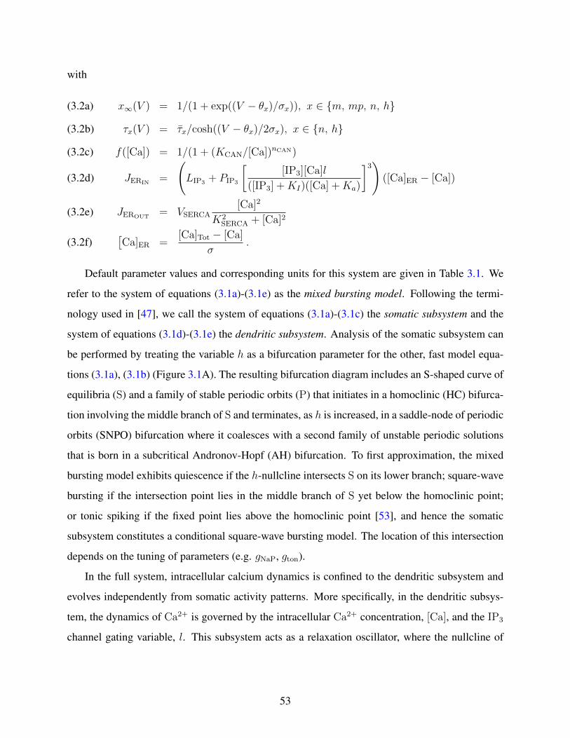
with
x∞(V ) = 1/(1 + exp((V − θx)/σx)), x ∈ {m, mp, n, h}(3.2a)
τx(V ) = τx/cosh((V − θx)/2σx), x ∈ {n, h}(3.2b)
f([Ca]) = 1/(1 + (KCAN/[Ca])nCAN)(3.2c)
JERIN=
(LIP3 + PIP3
[[IP3][Ca]l
([IP3] +KI)([Ca] +Ka)
]3)([Ca]ER − [Ca])(3.2d)
JEROUT= VSERCA
[Ca]2
K2SERCA + [Ca]2
(3.2e)
[Ca]ER =
[Ca]Tot − [Ca]
σ.(3.2f)
Default parameter values and corresponding units for this system are given in Table 3.1. We
refer to the system of equations (3.1a)-(3.1e) as the mixed bursting model. Following the termi-
nology used in [47], we call the system of equations (3.1a)-(3.1c) the somatic subsystem and the
system of equations (3.1d)-(3.1e) the dendritic subsystem. Analysis of the somatic subsystem can
be performed by treating the variable h as a bifurcation parameter for the other, fast model equa-
tions (3.1a), (3.1b) (Figure 3.1A). The resulting bifurcation diagram includes an S-shaped curve of
equilibria (S) and a family of stable periodic orbits (P) that initiates in a homoclinic (HC) bifurca-
tion involving the middle branch of S and terminates, as h is increased, in a saddle-node of periodic
orbits (SNPO) bifurcation where it coalesces with a second family of unstable periodic solutions
that is born in a subcritical Andronov-Hopf (AH) bifurcation. To first approximation, the mixed
bursting model exhibits quiescence if the h-nullcline intersects S on its lower branch; square-wave
bursting if the intersection point lies in the middle branch of S yet below the homoclinic point;
or tonic spiking if the fixed point lies above the homoclinic point [53], and hence the somatic
subsystem constitutes a conditional square-wave bursting model. The location of this intersection
depends on the tuning of parameters (e.g. gNaP, gton).
In the full system, intracellular calcium dynamics is confined to the dendritic subsystem and
evolves independently from somatic activity patterns. More specifically, in the dendritic subsys-
tem, the dynamics of Ca2+ is governed by the intracellular Ca2+ concentration, [Ca], and the IP3
channel gating variable, l. This subsystem acts as a relaxation oscillator, where the nullcline of
53

Table 3.1: The values of the parameters in the pre-BotC model given by equations (3.1) and (3.2)
Parameter valuesCm 21 pF gNa 28 nS σh 5 mV LIP3
0.37 pL ·ms−1
VNa 50 mV gK 11.2 nS τn 10 ms PIP331, 000 pL ·ms−1
VK −85 mV gL 11.2 nS τh 10, 000 ms KI 1.0 µMVL −58 mV gNaP 1 nS KCAN 0.74 µM Ka 0.4 µMθm −34 mV gCAN 0.7 nS nCAN 0.97 VSERCA 400 aMol ·ms−1
θn −29 mV σm −5 mV [IP3] 0.95 µM KSERCA 0.2 µMθmp −40 mV σn −4 mV [Ca]Tot 1.25 µM A 0.005 µM−1 ·ms−1
θh −48 mV σmp −6 mV KCa 0.000025 pL−1 Kd 0.4 µMσ 0.185
−2 −1 0 1 2
−40
−20
0
20
h
V
homoclinic
fixed point
AH
P (periodics)
S (equilibria)
h − nullcline
(A)
0.2 0.4 0.6 0.8
0.5
0.6
0.7
0.8
0.9
[Ca]
l
(B)
Figure 3.1: Basic structures of the two subsystems (3.1a)-(3.1c) and (3.1d)-(3.1e) with parameter
values as given in Table 3.1 but without coupling. (A): Projection onto (h, V )-space of the bifur-
cation diagram for the somatic subsystem along with the h-nullcline shown in cyan. The curve S
(black) denotes the fixed points of the equations (3.1a)-(3.1b) with h taken as a constant param-
eter, and the blue curve shows the maximum and minimum V along the family of periodics (P).
(B): Nullclines of [Ca] (red) and l (cyan) for the dendritic subsystem (3.1d)-(3.1e). The attracting
periodic orbit for this subsystem is shown in black.
[Ca] is a cubic curve and that of l is sigmoidal (Figure 3.1B). The dynamics of ([Ca], l) affects the
dynamics of (V, n, h); the parameter gCAN controls the coupling strength.
Similarly to the TB model [73], this model can produce two types of intrinsic bursting behav-
54

iors, depending on chosen parameter values. One type of bursting (somatic bursting) depends on
persistent sodium current inactivation, whereas the other type (dendritic bursting) relies on intra-
cellular Ca2+. [IP3] and gNaP are two critical parameters that can be used to switch the bursting
mechanism from one type to the other [47, 73]. Specifically, the level of [IP3] determines whether
the ([Ca], l) system exhibits a stable steady state or a stable periodic orbit, while [Ca] and gNaP both
affect the shape of the bifurcation diagram of the somatic subsystem. In the two extreme cases,
bursting is driven by either somatic membrane properties or Ca2+ oscillations alone. However,
in some region of (gNaP, [IP3]) parameter space, these mechanisms interact to produce a hybrid
bursting pattern called somato-dendritic bursting. Figure 3.2 shows the three types of bursting.
One of the most interesting somato-dendritic bursting solution patterns presented in [47] is
generated when [IP3] = 0.95 and gNaP = 2 (Figure 3.2, bottom panel). This pattern consists
of long bursts separated by sequences of short bursts and is observed experimentally [14]. For
convenience, we refer to such solutions as mixed bursting (MB) solutions. Numerical simulations
show that MB solutions are quite sensitive to changes of values of parameters such as [IP3] and
gNaP, to changes of timescale parameters, and to changes in timescale separation.
Since a regular bursting solution requires at least two timescales, it is natural to expect that
MB solutions, which involve a temporal progression of bursts, might need a third timescale. In
this chapter, we aim to better understand the mechanisms underlying the dynamics of the MB so-
lution [47] and to determine what mix of timescales is involved in generating this solution. More
generally, we seek to analyze what combinations of timescales can support MB solutions and
whether the mixed bursting model can be tuned to make the MB solution more robust, correspond-
ing to the fact that is seen in experiments [14]. With this goal, we will nondimensionalize to reveal
the presence of different timescales; determine how to group the timescales that are present (in
particular, whether to use two or three classes); use geometric singular perturbation theory to set
up reduced systems based on separation of timescales; and use the reduced systems to explain the
mechanisms underlying the dynamics of MB solutions.
By uncovering the mechanisms underlying the MB solution pattern in the mixed bursting
model, we deduce what combination of timescales can generally support MB solutions and con-
clude that a third timescale is not required to generate MB solutions in this model. In the course of
our analysis, we also attain important insights into how the mixed bursting model can be tuned to
55
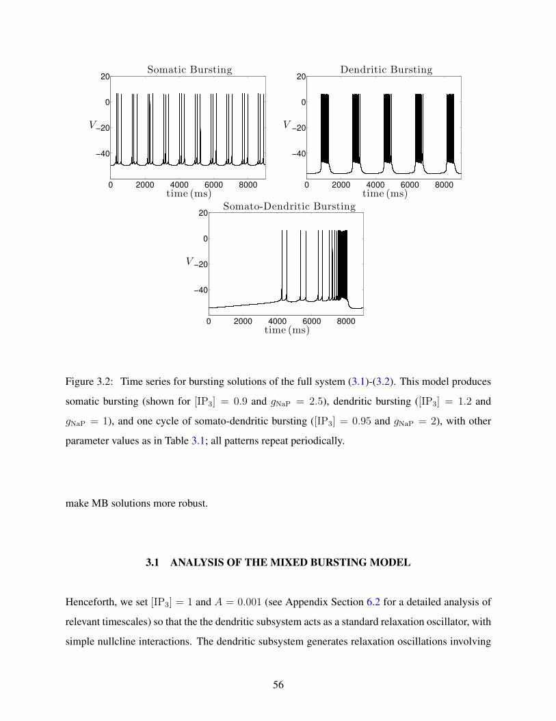
0 2000 4000 6000 8000
−40
−20
0
20
time (ms)
V
Somatic Bursting
0 2000 4000 6000 8000
−40
−20
0
20
time (ms)
V
Dendritic Bursting
0 2000 4000 6000 8000
−40
−20
0
20
time (ms)
V
Somato-Dendritic Bursting
Figure 3.2: Time series for bursting solutions of the full system (3.1)-(3.2). This model produces
somatic bursting (shown for [IP3] = 0.9 and gNaP = 2.5), dendritic bursting ([IP3] = 1.2 and
gNaP = 1), and one cycle of somato-dendritic bursting ([IP3] = 0.95 and gNaP = 2), with other
parameter values as in Table 3.1; all patterns repeat periodically.
make MB solutions more robust.
3.1 ANALYSIS OF THE MIXED BURSTING MODEL
Henceforth, we set [IP3] = 1 and A = 0.001 (see Appendix Section 6.2 for a detailed analysis of
relevant timescales) so that the the dendritic subsystem acts as a standard relaxation oscillator, with
simple nullcline interactions. The dendritic subsystem generates relaxation oscillations involving
56

jumps in [Ca] between branches of the [Ca]-nullcline alternating with drift in ([Ca], l) along these
branches (Figure 3.3); the [Ca]-jumps are fast relative to the drift. Under this new choice of
parameter values, there is a clear separation of timescales between V (fast), [Ca] (slow) and l
(superslow). To apply standard tools of geometric singular perturbation theory, we also need a
clear separation of timescales between n, h and the other variables. However, this separation is
lacking, since the rate factors multiplying the equations for the gating variables depend on the
voltage. Unitl we resolve this issue, we temporarily group n as a fast variable and h as a slow
variable, as has been suggested in past studies of the Butera model, such as [2].
0 0.2 0.4 0.6 0.8 1
0.5
0.6
0.7
0.8
0.9
1
[Ca]
l1©
2©
3©
4©
Figure 3.3: Attracting dynamics in ([Ca], l)-space, with parameter values given in Table 3.1 except
[IP3] = 1 and A = 0.001. The red curve is the [Ca]-nullcline and the cyan curve is the l-nullcline.
The hollow square denotes the equilibrium solution, which is a source. The attracting periodic orbit
for the dendritic subsystem is shown in black (with clockwise flow passing through the numbered
regions in increasing order). Yellow symbols mark key points along the solution trajectory (star:
start of phase 1©; circle: start of phase 2©; square: start of phase 3©; triangle: start of phase 4©).
To explain the mechanisms underlying the dynamics of the mixed bursting model (3.1), we
link various two-dimensional projections, each corresponding either to a bifurcation diagram with
respect to some parameter or to the phase plane of one oscillator. Since ([Ca], l) oscillates in-
dependently of (V, n, h), it is useful to consider the system from the perspective of a fast-slow
system driven by a slow-superslow oscillation (cf. [41]). There are three slow/superslow variables,
57
h, [Ca], l, in the full system. Changes in l affect the somatic subsystem (3.1a)-(3.1c) indirectly,
through the coupling between [Ca] and l and the coupling of [Ca] to V , but not directly. Thus, if
we treat all slow or superslow variables as bifurcation parameters, then it is sufficient to consider
only h and [Ca] when studying the dynamics of the somatic subsystem [47]. With these two pa-
rameters, it is convenient to treat h as a bifurcation parameter for the geometric analysis of the
somatic subsystem and to consider the effect of [Ca] on the resulting bifurcation diagram. Instead
of using [Ca] directly, we follow [47] and choose gCANTot= gCANf([Ca]) as a bifurcation pa-
rameter, where f([Ca]) is the concave down and monotonically increasing function of [Ca] given
in equation (3.2c). Before we actually implement the analysis, however, we will perform some
helpful pre-processing of the equations.
3.1.1 Rescaling and simplification of timescales
Our analysis will depend heavily on exploiting the presence of different timescales. As a first step,
it is helpful to rescale the variables so that the important timescales can be explicitly identified. To
this end, we define new dimensionless variables (v, c, τ), and voltage, calcium and timescales Qv,
Qc and Qt, respectively, such that:
(3.3) V = Qv · v , [Ca] = Qc · c , t = Qt · τ.
Note that n, h and l are already dimensionless in (3.1).
Details of the nondimensionalization procedure, including the determination of appropriate
values for Qv, Qc and Qt, are given in Appendix Section 6.3. From this process, we obtain a
dimensionless system of the form
58
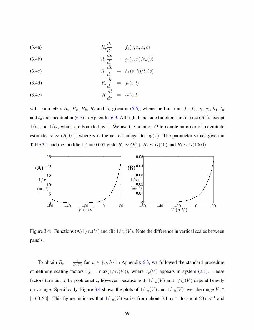
Rvdv
dτ= f1(v, n, h, c)(3.4a)
Rndn
dτ= g1(v, n)/tn(v)(3.4b)
Rhdh
dτ= h1(v, h)/th(v)(3.4c)
Rcdc
dτ= f2(c, l)(3.4d)
Rldl
dτ= g2(c, l)(3.4e)
with parameters Rv, Rn, Rh, Rc and Rl given in (6.6), where the functions f1, f2, g1, g2, h1, tn
and th are specified in (6.7) in Appendix 6.3. All right hand side functions are of size O(1), except
1/tn and 1/th, which are bounded by 1. We use the notation O to denote an order of magnitude
estimate: x ∼ O(10n), where n is the nearest integer to log(x). The parameter values given in
Table 3.1 and the modified A = 0.001 yield Rv ∼ O(1), Rc ∼ O(10) and Rl ∼ O(1000).
−60 −40 −20 0 200
5
10
15
20
25
V (mV)
1/τn
(ms−1)
(A)
−60 −40 −20 0 200
0.01
0.02
0.03
0.04
0.05
V (mV)
1/τh
(ms−1)
(B)
Figure 3.4: Functions (A) 1/τn(V ) and (B) 1/τh(V ). Note the difference in vertical scales between
panels.
To obtain Rx = 1Qt·Tx for x ∈ {n, h} in Appendix 6.3, we followed the standard procedure
of defining scaling factors Tx = max(1/τx(V )), where τx(V ) appears in system (3.1). These
factors turn out to be problematic, however, because both 1/τn(V ) and 1/τh(V ) depend heavily
on voltage. Specifically, Figure 3.4 shows the plots of 1/τn(V ) and 1/τh(V ) over the range V ∈[−60, 20]. This figure indicates that 1/τn(V ) varies from about 0.1 ms−1 to about 20 ms−1 and
59

1/τh(V ) varies from about 0.0001 ms−1 to about 0.04 ms−1. From the definition of Tx, we then
obtain Tn ≈ 20 ms−1 and Th ≈ 0.04 ms−1. As a result, the terms 1/tx(V ) =: 1/τx(V )Tx
appearing
on the right hand sides of the n and h equations in (3.4) vary from O(0.001) to O(1). However,
nondimensionlization requires the right hand sides to beO(1). Therefore, the quantitiesRn andRh,
based on Tn and Th, respectively, cannot capture the timescales for n and h. In other words, because
the evolution rates of n and h depend on voltage V (t), these variables will have different timescales
at different phases within a solution. As a first step in addressing this issue, we temporally reduce
the reliance of the timescales of n and h on voltage by setting the two functions τh(V ), τn(V ) in
(3.1) to be constants, τh, τn, respectively. As a result, we obtain the following dimensionless mixed
bursting model, which we call the constant-τ model:
Rvdv
dτ= f1(v, n, h, c)(3.5a)
Rndn
dτ= g1(v1, n)(3.5b)
Rhdh
dτ= h1(v1, h)(3.5c)
Rcdc
dτ= f2(c, l)(3.5d)
Rldl
dτ= g2(c, l)(3.5e)
with relative rates of all variables:
Rv = O(1), Rx =τxQt
= O(τx), x ∈ {n, h}(3.6a)
Rc = O(10), Rl = O(1000).(3.6b)
from which we conclude that v evolves on a fast timescale, c evolves on a slow timescale, and l
evolves on a superslow timescale for the baseline parameter values, although the values Rv, Rc
and Rl can be varied by changing Cm, KCa and A, respectively, as shown in (6.6) in Appendix
6.3. The constants τn and τh appearing in (3.6a), which control the timescales for n and h, will
need to be determined. As noted earlier, to analyze the dynamics of (3.5), our approach is to treat
h as a bifurcation parameter for the geometric analysis of the somatic subsystem (3.5a)-(3.5b)
and consider the effect of the dendritic system (c, l) on the resulting bifurcation diagram. In the
following, we will first determine what timescales for n and h, controlled by τn and τh, are needed
60

for (3.5) to generate an MB solution, while other timescales are as specified in (3.6); second, we
will ascertain which timescales can be combined without losing the qualitative features of MB
solutions; and third, we will deduce what combinations of timescales can support MB solutions in
general. For convenience, we henceforth omit units of parameter values.
3.1.2 Dynamics of the constant-τ model (3.5)
Based on simulations of (3.5) over a range of τn and τh values, we find that under the choice τn = 5
and τh = 1000, (3.5) yields an MB solution, the time series of which is shown in Figure 3.5A. In
this case, h evolves on a superslow timescale, comparable to l.
As a first step of analyzing such MB patterns, we investigate the coupling effect in (3.5). When
gcan = 0, the constant-τ model decouples into two systems, each of which has a multiple-timescale
structure. For the parameter values we have chosen, the bifurcation structure and the nullclines for
the uncoupled systems are qualitatively as shown in Figure 3.1. Since the coupling in our system is
unidirectional, the oscillations in (c, l) are independent of gcan and of the dynamics of the (v, n, h)
subsystem; they are standard relaxation oscillations consisting of a superslow excursion through
the silent phase (Figure 3.3, 1©), a slow jump away from the c-nullcline up to the active phase
(Figure 3.3, 2©), a superslow excursion through the active phase (Figure 3.3, 3©), and a slow jump
back to the silent phase (Figure 3.3, 4©). In contrast, if gcan > 0, then the (v, n, h) subsystem
depends on gcan and on the (c, l) oscillation. With the choice of gcan = 0.7, the constant-τ model
can generate an MB solution. An example of the coupling effect can be seen in Figure 3.5B:
the magenta (resp. blue) curve denotes the bifurcation diagram of the somatic subsystem that is
obtained for c at 0.0171 (resp. 1) and we can see that as c increases, the bifurcation diagram will
shift down and to the left.
In the following, we will first explain the mechanism underlying the small bursts in the MB
solution ([53], [26]) and then elucidate how the transition to a long burst occurs, from the perspec-
tive of how the somatic subsystem is driven by the dendritic subsystem. The use of this kind of
perspective has proved helpful in past analyses of various models with two timescales as well as
of a three timescale model [41].
In Figure 3.5C, we project the first small burst solution and the bifurcation diagram of the
61

0 2000 4000 6000 8000
−0.5
0
0.5
Time(ms)
v
(A)
−3 −2 −1 0 1 2
−0.4
−0.2
0
0.2
0.4
h
v
c increases
(B)
0.3 0.4 0.5 0.6
−0.4
−0.2
0
0.2
0.4
h
v
(C)
0 0.2 0.4 0.60
0.1
0.2
0.3
0.4
h
gCANtot
1©
2©
3©
4©
HCLF
(D)
Figure 3.5: Simulation of the MB solution generated by (3.5), together with corresponding bifur-
cation diagrams, for τn = 5, τh = 1000, [IP3] = 1, A = 0.001, and other parameter values as given
in Table 3.1. Circled numbers and yellow symbols correspond to phases of the (c, l) oscillation
and the points of transition between them, as shown in Figure 3.3. (A): Temporal evolution of v.
(B): The effect of c on the bifurcation diagram for the (v, n) system, projected into (h, v)-space,
along with the h-nullcline (cyan). Increasing c from 0.0171 to 1 results in a shift of the bifur-
cation diagram to the left (magenta to blue) and switches the homoclinic bifurcation to a SNIC.
(C): Projection of the first small burst in the MB solution from (A) onto the bifurcation diagram
(with c = 0.0171) in (h, v)-space, along with the h-nullcline (cyan). The blue and red dashed lines
indicate the h values where the lower fold and homoclinic bifurcations occur, respectively. (D):
Homoclinic bifurcation curve (red), the curve of saddle-node bifurcations corresponding to the
lower fold of the bifurcation diagram (blue) and the trajectory (black) in (h, gCANTot) parameter
space.
62
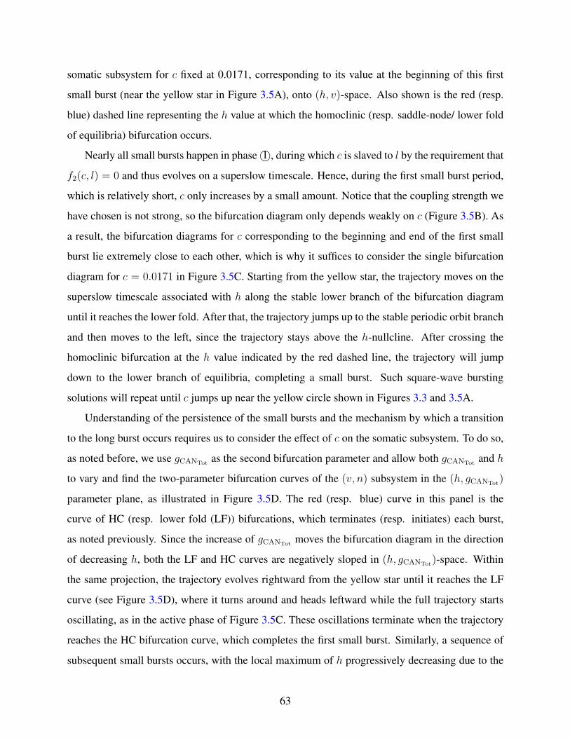
somatic subsystem for c fixed at 0.0171, corresponding to its value at the beginning of this first
small burst (near the yellow star in Figure 3.5A), onto (h, v)-space. Also shown is the red (resp.
blue) dashed line representing the h value at which the homoclinic (resp. saddle-node/ lower fold
of equilibria) bifurcation occurs.
Nearly all small bursts happen in phase 1©, during which c is slaved to l by the requirement that
f2(c, l) = 0 and thus evolves on a superslow timescale. Hence, during the first small burst period,
which is relatively short, c only increases by a small amount. Notice that the coupling strength we
have chosen is not strong, so the bifurcation diagram only depends weakly on c (Figure 3.5B). As
a result, the bifurcation diagrams for c corresponding to the beginning and end of the first small
burst lie extremely close to each other, which is why it suffices to consider the single bifurcation
diagram for c = 0.0171 in Figure 3.5C. Starting from the yellow star, the trajectory moves on the
superslow timescale associated with h along the stable lower branch of the bifurcation diagram
until it reaches the lower fold. After that, the trajectory jumps up to the stable periodic orbit branch
and then moves to the left, since the trajectory stays above the h-nullcline. After crossing the
homoclinic bifurcation at the h value indicated by the red dashed line, the trajectory will jump
down to the lower branch of equilibria, completing a small burst. Such square-wave bursting
solutions will repeat until c jumps up near the yellow circle shown in Figures 3.3 and 3.5A.
Understanding of the persistence of the small bursts and the mechanism by which a transition
to the long burst occurs requires us to consider the effect of c on the somatic subsystem. To do so,
as noted before, we use gCANTotas the second bifurcation parameter and allow both gCANTot
and h
to vary and find the two-parameter bifurcation curves of the (v, n) subsystem in the (h, gCANTot)
parameter plane, as illustrated in Figure 3.5D. The red (resp. blue) curve in this panel is the
curve of HC (resp. lower fold (LF)) bifurcations, which terminates (resp. initiates) each burst,
as noted previously. Since the increase of gCANTotmoves the bifurcation diagram in the direction
of decreasing h, both the LF and HC curves are negatively sloped in (h, gCANTot)-space. Within
the same projection, the trajectory evolves rightward from the yellow star until it reaches the LF
curve (see Figure 3.5D), where it turns around and heads leftward while the full trajectory starts
oscillating, as in the active phase of Figure 3.5C. These oscillations terminate when the trajectory
reaches the HC bifurcation curve, which completes the first small burst. Similarly, a sequence of
subsequent small bursts occurs, with the local maximum of h progressively decreasing due to the
63

left drift of LF as gCANTotincreases on the superslow timescale. The fact that the trajectory in
(h, gCANTot)-space reaches the LF and HC curves six times before gCANTot
jumps up corresponds
to the existence of the six small bursts (see Figure 3.5A). In fact, since the l-nullcline lies close to
the left knee of the c-nullcline, as discussed in the Remark of Appendix Section 6.2, the jump up
is gradual; a seventh small burst actually occurs during the initial part of the jump up (just after the
yellow circle in Figure 3.5A) and is followed by the start of an eighth small burst. In the singular
limit, however, this additional bursting will be lost and all small bursts will occur within phase 1©.
As the trajectory passes the yellow circle and moves into phase 2©, f2 = 0 no longer applies,
and the flow switches from superslow to slow. More precisely, the gCANTotcoordinate starts to
jump up on the slow timescale, while h remains on the superslow timescale. During this jump up
in phase 2© (from circle to square), the LF and HC curves will meet at some point, coalescing to
form a SNIC bifurcation curve; since the oscillation frequency goes to 0 as a SNIC is approached,
as with the HC, we color the SNIC curve red in Figure 3.5D. As c jumps up and pulls the trajectory
farther away from the SNIC curve, there is a burst of higher frequency spiking. This spiking results
because h, which is evolving superslowly, remains almost constant during phase 2©, relative to the
decrease of the h-coordinate of the SNIC bifurcation due to the slow jump up of c, and hence
the trajectory is now oscillating somewhere relatively far from the SNIC curve (see the yellow
square in Figure 3.5D); in this system, the farther the trajectory is from the SNIC, the higher its
spiking frequency. We thus obtain spiking with high frequency at the start of phase 3© (yellow
square), after which the frequency gradually decreases as the trajectory moves closer to SNIC on
the superslow timescale.
Besides the change in frequency, the amplitude of the v spikes increases progressively during
phase 3©. This feature results from the structure of the somatic system bifurcation diagram: pe-
riodic orbit amplitudes start small at the AH bifurcation (large h) and keep increasing as h gets
closer to the SNIC bifurcation (Figure 3.5B). The bifurcation diagram moves to the leftmost posi-
tion as c reaches its maximum value (blue curve in Figure 3.5B), at which h is around 0.4 (yellow
square in Figure 3.5D). Hence, at the start of phase 3©, the trajectory is oscillating in the middle of
the periodic orbit branch, somewhere far from the SNIC bifurcation, resulting in spiking with low
amplitude. As c decreases on the superslow timescale during phase 3©, it shifts the corresponding
bifurcation diagram to the right. Meanwhile, the trajectory moves in the direction of deceasing h
64

(Figure 3.5D). As a result, the periodic orbits that shape the v spikes are progressively closer to the
SNIC bifurcation, and hence these spikes feature increasing amplitude as phase 3© progresses.
As phase 4© begins, c no longer tracks l on the superslow timescale and instead evolves on the
slow timescale, just as during phase 2©. Hence, the slow jump down in cwill bring the trajectory far
below the HC/SNIC curve, so the trajectory enters the silent phase and the long burst terminates.
As the solution finally returns to our starting point (star in Figure 3.5A and D), one cycle of the
MB solution is completed.
Besides describing the dynamic mechanisms underlying MB solutions, our goal is to determine
what mix of timescales is involved in the MB pattern. In the following, we separate the MB solution
into three phases, denoted by the quiescence (Q) phase, the square-wave bursting (SW) phase, and
the long bursting (LB) phase, respectively. Below are the three conditions drawn from the above
analysis that together support the MB solution:
(C1): It is necessary that the somatic subsystem acts as a square-wave burster for c values arising dur-
ing the SW phase, so that there exist small burst solutions before c jumps up to its active phase.
In other words, there must be a gap in h between the LF and HC curves in the (h, gCANTot)
parameter plane for c small (Figure 3.5D).
(C2): The trajectory needs to cross the gap between the LF and HC curves multiple times, with each
crossing taking long enough to allow for a square-wave burst, so that there are multiple small
bursts before the long burst; the timescales of h, v, and c should be related during the SW
phase in a way that makes outcome possible.
(C3): The transition to the long burst occurs due to the jump up of c to the active phase, which
requires the timescale for c to become faster than h and l after the SW phase.
We use these three conditions to find the right combination of timescales that are generally
needed to obtain an MB solution.
3.1.3 Finding the combination of timescales that supports MB solutions in the constant-τ
model (3.5)
3.1.3.1 (C1) ⇒ Analysis of timescales of v and n (C1) requires that the (v, n, h) subsystem
acts as a square-wave burster for c small, which is determined by the bifurcation diagram of the
65

(v, n) subsystem with h treated as a bifurcation parameter. Note that the AH value and the position
of the periodic orbit (P) branch of the bifurcation diagram for (v, n) depend on Rv and Rn, which
determine the timescales of v and n. Thus, we investigate what mix of timescales for these two
variables is needed.
Recall that Rv and Rn can be varied by changing the two parameters Cm and τn, respectively.
In the following, we fixCm = 21 and vary τn to study how it will affect the bifurcation diagram and
under what condition the somatic subsystem can generate a square-wave bursting solution. Repre-
sentative results are shown in Figure 3.6A, where the bifurcation diagram of the (v, n) subsystem
with respect to h for c = 0.0171 is computed. While the curve of equilibria of the (v, n) subsystem,
S (black), and the h-nullcline (cyan) are both independent of τn, the periodic orbit branch, P, is
sensitive to changes of τn. Specifically, an increase of τn moves the family of periodic orbits to the
right in (h, v)-space (Figure 3.6A).
−2 −1 0 1
−0.6
0
0.4
h
v
τn = 1
τn = 5
τn = 10
(A)
0 0.2 0.4 0.60
0.1
0.2
0.3
h
gCANtot
HC (τn = 5)HC (τn = 10LF (τn = 5, 10)
(B)
Figure 3.6: Bifurcation diagrams for the somatic subsystem for various τn values. (A): Bifurcation
diagrams for the somatic subsystem with h as a parameter and c fixed at 0.0171. From the magenta
curve to the blue to the red, τn varies from 1 to 5 to 10. As τn increases, AH and P move to the
upper right, while the h-nullcline (cyan) and S (black) remain unchanged. (B): Two curves of HC
bifurcations (red, τn = 5; green, τn=10) and two curves of LF bifurcations for τn = 5 and 10, both
overlapping with the green curve, in (h, gCANTot) parameter space. The horizontal line represents
gCANTot= 0.116, where the green and red curves meet.
For τn = 1, as h is decreased, there is a family of small amplitude unstable periodic orbits
created in a HC bifurcation involving the middle branch of equilibria S, which terminates when
66

it coalesces in a SNPO bifurcation with a second family of stable periodic solutions born in a
supercritical AH bifurcation on the upper branch of equilibria, as illustrated by the magenta curve
in Figure 3.6A. In this case, the MB solution does not exist. In fact, under such a choice, the
constant-τ model yields a solution lacking v spiking. For c at its minimum, the h-nullcline and the
equilibria branch S intersect at one stable fixed point on the upper branch of S and two unstable
fixed points on the middle branch (see Figure 3.6A). Notice that the increase of c, which moves
S (black) and P (magenta) to the left, will not change the stability of the equilibrium point on the
upper branch of S. Hence, for the full range of c values, there is a stable equilibrium of (v, n, h),
and the trajectory will eventually be attracted by this family of stable equilibria, yielding the plateau
of v.
For τn = 5 (resp. τn = 10) and c = 0.0171, the periodic orbit branch is given by the blue (resp.
red) curve in Figure 3.6A. In both cases, unlike when τn = 1, as h is increased, a stable family
of periodic orbits is created in a HC bifurcation involving the middle branch of S and is destroyed
in a supercritical AH bifurcation along the upper branch. Although these two stable periodic orbit
branches appear to be quite similar, there is a crucial difference between them. For τn = 10, there
is a SNIC bifurcation as the HC bifurcation meets with the LF bifurcation for c at its minimal
value and this bifurcation persists for all c values within a complete relaxation oscillation cycle
(see Figure 3.6B). Thus there is only a tonic spiking solution, which violates (C1). For τn = 5,
there is a gap in h between the LF and HC curves for c = 0.0171 (Figure 3.6A), persisting up to
roughly c = 0.14 (Figure 3.6B), which will result in a square-wave bursting solution as required.
Therefore, τn = 5 together with Cm = 21 is a parameter set that satisfies (C1).
In summary, among all three cases that we have discussed above, only τn = 5 (Rn = 5) can
support the MB solution. Recall that we have chosen the timescale of voltage to be Rv ∼ O(1). To
determine whether v and n truly can be coordinated as evolving on disparate timescales, a natural
question to ask is: can we make the timescales of v and n more separated without losing the MB
solution? To figure this out, we now fix τn = 5 and allow both Cm and h to vary to find the somatic
(v, n) subsystem bifurcation curves in the (Cm, h) parameter plane, as illustrated in Figure 3.7.
The LF and HC curves are shown in blue and red, respectively, and the green curve denotes the
AH bifurcation on the upper branch of S.
For Cm sufficient large (e.g., 200), as h is increased, there is a branch of unstable small ampli-
67
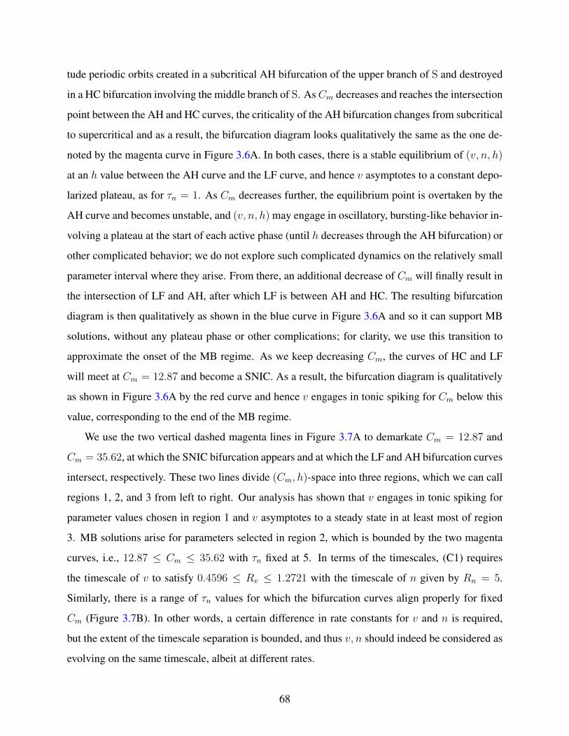
tude periodic orbits created in a subcritical AH bifurcation of the upper branch of S and destroyed
in a HC bifurcation involving the middle branch of S. AsCm decreases and reaches the intersection
point between the AH and HC curves, the criticality of the AH bifurcation changes from subcritical
to supercritical and as a result, the bifurcation diagram looks qualitatively the same as the one de-
noted by the magenta curve in Figure 3.6A. In both cases, there is a stable equilibrium of (v, n, h)
at an h value between the AH curve and the LF curve, and hence v asymptotes to a constant depo-
larized plateau, as for τn = 1. As Cm decreases further, the equilibrium point is overtaken by the
AH curve and becomes unstable, and (v, n, h) may engage in oscillatory, bursting-like behavior in-
volving a plateau at the start of each active phase (until h decreases through the AH bifurcation) or
other complicated behavior; we do not explore such complicated dynamics on the relatively small
parameter interval where they arise. From there, an additional decrease of Cm will finally result in
the intersection of LF and AH, after which LF is between AH and HC. The resulting bifurcation
diagram is then qualitatively as shown in the blue curve in Figure 3.6A and so it can support MB
solutions, without any plateau phase or other complications; for clarity, we use this transition to
approximate the onset of the MB regime. As we keep decreasing Cm, the curves of HC and LF
will meet at Cm = 12.87 and become a SNIC. As a result, the bifurcation diagram is qualitatively
as shown in Figure 3.6A by the red curve and hence v engages in tonic spiking for Cm below this
value, corresponding to the end of the MB regime.
We use the two vertical dashed magenta lines in Figure 3.7A to demarkate Cm = 12.87 and
Cm = 35.62, at which the SNIC bifurcation appears and at which the LF and AH bifurcation curves
intersect, respectively. These two lines divide (Cm, h)-space into three regions, which we can call
regions 1, 2, and 3 from left to right. Our analysis has shown that v engages in tonic spiking for
parameter values chosen in region 1 and v asymptotes to a steady state in at least most of region
3. MB solutions arise for parameters selected in region 2, which is bounded by the two magenta
curves, i.e., 12.87 ≤ Cm ≤ 35.62 with τn fixed at 5. In terms of the timescales, (C1) requires
the timescale of v to satisfy 0.4596 ≤ Rv ≤ 1.2721 with the timescale of n given by Rn = 5.
Similarly, there is a range of τn values for which the bifurcation curves align properly for fixed
Cm (Figure 3.7B). In other words, a certain difference in rate constants for v and n is required,
but the extent of the timescale separation is bounded, and thus v, n should indeed be considered as
evolving on the same timescale, albeit at different rates.
68

0 100 200 300
−2
−1
0
1
Rn = 5
Cm
h
Rv = 0.4596
Rv = 1.2721
1 2 3
LF
HCAH
(A)
0 10 20 30 40
−1
0
1
Rv = 1
τn
h
3 2 1
Rn = 2.909
Rn = 8.116
AH
HC
LF(B)
Figure 3.7: Bifurcation curves for the (v, n) subsystem of (3.5) for c = 0. The curves of AH
bifurcations, LF bifurcations and HC bifurcations are given by the green, blue and red curves,
respectively. Solid (resp., dashed) black curves indicate stable (resp., unstable) equilibria of the
somatic subsystem. (C1) requires that for fixed Cm, the curves progress from red to blue to green
as h increases. (A): (Cm, h) parameter space with τn = 5. The two magenta vertical lines represent
Cm = 12.87 and Cm = 35.62, at which the LF and HC bifurcation curves intersect and the LF and
AH bifurcation curves intersect, respectively. (B): (τn, h) parameter space with Cm = 21. The two
magenta vertical lines represent τn = 2.909 and τn = 8.116, with similar interpretations as in (A).
3.1.3.2 (C2) and (C3)⇒ Analysis of timescales of h, v2 and w Using (C2) and (C3), we can
obtain the relation among timescales for the other three variables, h, c and l, required to yield an
MB solution. Imposing (C3), we require that the (c, l) system acts as a relaxation oscillator and
so the timescale of c is determined by that of l during its silent phase. In other words, we have
Rc ≈ Rl during phase 1© and phase 3©. Moreover, the fact that almost all small bursts happen
during phase 1© suggests that the SW phase lies in phase 1©. As a result, for (C2), we compare Rh
with Rl, rather than Rc, during phase 1©.
Based on (C1), (C3), and (3.6), we set the timescales to be (Rv, Rn) ∼ (1, 5) and (Rc, Rl) ∼(10, 1000), respectively. Next we consider (C2). By fixing Rl = 1000 and varying τh, which
controls Rh, we study the influence of the relation between Rh and Rl on the dynamics of (3.5).
From numerical simulations over a range of τh values, we find that (3.5) can generate MB solutions
69

when τh = 1000, but this pattern is lost when τh = 90 (Figure 3.8A) or τh = 10000 (Figure 3.8B).
These numerical results suggest that h and l may need to evolve at comparable rates in order for
the constant-τ model to generate MB solutions.
The top row in Figure 3.8 shows the time series for v, while the bottom row shows the two-
parameter bifurcation diagrams in (h, gCANTot)-space together with the projection of the solution
shown in the top row. The left panel of Figure 3.8 shows the case when Rh = 90 < Rl = 1000
during phase 1©. Since c is slaved to l in this phase, h is evolving faster than c and thus the
trajectory crosses the curves of LF and HC bifurcations within only one spike. This process will
continue until c jumps up to its maximum value (yellow square), after which a burst of higher
frequency spiking begins via the mechanism discussed in Section 3.1.2 and terminates when c falls
down during phase 4©. Therefore, the spiking persists throughout the c oscillation, failing to yield
an MB solution. In the other case, when h evolves on a timescale of O(10000), h is slower than l
and c, and (3.5) generates a bursting solution as shown in Figure 3.8B. This solution arises because
the drift of the trajectory in the direction of decreasing h after passing the curve of LF bifurcations
is too slow for the solution to reach the curve of HC bifurcations (see Figure 3.8D). As a result,
spiking continues throughout the silent and active phases of the (c, l) oscillation, corresponding to
a single burst active phase, until the slow jump down of c during phase 4© brings the flow below
the HC curve, terminating the burst of v spiking. On the other hand, if we fix Rh = 1000 and
slow down l (e.g., Rl = 10000), the MB solution persists, with more small bursts produced within
each MB cycle because phase 1©, during which small bursts occur, is prolonged. Therefore, we
conclude that for mixed bursting, the timescales should satisfy the following refined and extended
version of condition (C2):
(C2)’: The trajectory needs to cross the gap between the LF and HC curves multiple times, with each
crossing taking long enough to allow for a square-wave burst, so that there are multiple small
bursts before the long burst; for this to happen, h should be slow enough relative to v and n,
and c should evolve at least as slowly as h during the SW phase.
For the above analysis to apply, we require that c evolves faster than h and l, but we have not
yet specified how fast. The discussion up to this point shows that if (C3) holds and we speed up c,
then we do not affect (C1), (C2)’, or (C3). In fact, as long as the relaxation character of the (c, l)
70

s
0 2000 4000 6000 8000
−0.5
0
0.5
Time(ms)
v
(A)
0 2000 4000 6000 8000
−0.5
0
0.5
Time(ms)
v
(B)
0 0.2 0.4 0.6
0.1
0.2
0.3
0.4
h
gCANtot
(C)
0 0.2 0.4 0.6
0.1
0.2
0.3
0.4
h
gCANtot
1©
2©
3©
4©
(D)
Figure 3.8: Time series for attracting solutions of the constant-τ model and associated bifurcation
diagrams when Rv = 1, Rn = 5, Rc = 10, and Rl = 1000. In (A) and (C), Rh = 90, (B) and
(D): Rh = 10000. Top row shows temporal evolution of v (black); bottom row shows the curves of
HC bifurcations (red), LF bifurcations (blue) and the trajectory (black), projected into (h, gCANTot)
parameter space. The yellow symbols indicate transition points between different phases for the
dendritic subsystem, as shown in Figure 3.3. Circled numbers in (D), which represent the four
phases of the (c, l) oscillation as in Figure 3.3, are omitted in (C).
oscillations is maintained, the timescale of c, which determines how fast the jump up of c happens
and hence determines how fast the transition from the small burst to the long burst occurs, will
not affect the MB pattern qualitatively. This claim is supported by the simulation result that if we
make Rc ∼ O(1) = Rv so that c evolves on the same timescale as v, the MB pattern still occurs.
We summarize the choices about the timescales that support MB dynamics in Table 3.2, from
71

which we observe that there are three different orders of magnitude present. If MBs are truly a three
timescale form of dynamics, then we should be able to separate these three classes as much as we
like while still maintaining the MB solution. However, this is not the case. In fact, the MB solution
breaks down as we make (v, c) and n more separated. Hence, in a timescale decomposition, the
timescales should be considered as segregating into two classes. This grouping is supported by the
fact that as we exaggerate the separation between these two classes, the MB solution still exists.
Therefore, we conclude that the MB solution of the constant-τ model (3.5) is not specifically a
three timescale phenomenon.
Table 3.2: Timescales for the constant-τ model (3.5)
Fast Slow
Rv Rn Rc Rh Rl
(0.4596, 1.2721) 5 (0.4596, 5) 1000 ≥ 1000
3.1.4 Dynamics of the mixed bursting model (3.1)
In this subsection, we will first use the approach that was applied in Section 3.1.2 to explain the
mechanisms underlying MB solutions of (3.1) with parameters given by Table 3.1. After that,
we will analyze what mix of timescales can support MB solutions and how timescales should
be grouped to apply geometric singular perturbation theory. Finally, recalling that MB solutions
generated by the system (3.1) for its original parameter values are very sensitive to changes in
parameters, we will investigate how the timescales of the mixed bursting model can be tuned to
make the MB solutions more robust, reflecting the fact that they are observed experimentally [14].
Based on the timescales that we have found in Section 3.1.3, we can now modify the original
mixed bursting model (3.1), the dimensionless version of which is given by (3.4), to obtain MB
solutions. Notice that the only difference between the fmixed bursting model and the constant-τ
model is whether the timescales of n and h are the v-dependent functions τn(v) and τh(v) or the
constants τn and τh. We set Rc = O(1) by increasing KCa from 2.5e − 5 to 1.25e − 4 and keep
timescales for v and l unchanged so that we have (Rv, Rc, Rl) = (O(1), O(1), O(1000). According
72

to Table 3.2, we will need to modify τn(v) and τh(v) in order to obtain Rn ≈ 5 and Rh ≈ 1000 for
MB solutions. Specifically, we require these two functions to be less dependent on v and so as close
as possible to the size 5 or 1000. To this end, we introduce a new parameter ax with default value
0 and abuse notation to redefine 1/τx(V ) = τx/cosh((V − θx)/2σx) + ax, where x ∈ {n, h}. We
constrain the timescales for n and h by varying the parameters (σn, an) and (σh, ah), respectively.
−0.5 −0.3 −0.1 0.1
0.1
2.5
v
1/τn
Rn ≈ 5
σn = −5, an = 0.1σn = −6, an = 0.1
(A)
−0.5 −0.3 −0.1 0.10
0.005
0.01
0.015
0.02
v
1/τh
Rh ∼ O(1000)
σh = 7, ah = 0.001
(B)
Figure 3.9: The graphs of the functions 1/τn(v) and 1/τh(v), with both default and new choices of
σn, an, σh and ah. (A): The graph of 1/τn(v) for the default parameter values (σn, an) = (−4, 0)
(dashed blue), or for the modified parameter values (σn, an) = (−5, 0.1) (green) or (σn, an) =
(−6, 0.1) (magenta). (B): The graph of 1/τh(v) for the default parameter value (σh, ah) = (5, 0)
(dashed blue), or for the modified parameter value (σh, ah) = (7, 0.001) (red).
In Figure 3.9, we plot both the original τx functions and their modified versions with the new
parameters we have chosen. The reciprocals of the original τn and τh functions are given by the
dashed blue curves, while the reciprocals of the modified functions that are now less dependent on
voltage are denoted by the solid curves. To understand the effects of modifying τn on the robustness
of MB solutions, we consider two examples of τn(v), the reciprocals of which are shown in Figure
3.9A. In the case when σn = −6, the upper branch of somatic subsystem equilibria (magenta)
intersects the h-nullcline (cyan) at a stable fixed point (Figure 3.10), leading to a bistability of
silence and bursting and hence compromising the robustness of the bursting solution. There is no
such issue in the other case, when σn = −5. In fact, the resulting bifurcation diagram (Figure 3.10,
green) is qualitatively the same as the one denoted by the blue curve in Figure 3.6A except that the
AH bifurcation on the upper branch of S is now subcritical, and so we choose to modify τn(v) with
73

σn = −0.5, an = 0.1.
−2 −1 0 1
−0.5
−0.3
−0.1
0.1
h
v
Figure 3.10: The bifurcation diagrams of the somatic subsystem corresponding to the modified
forms of τn(v) as shown in Figure 3.9A, along with the h-nullcline (cyan). The other color codings
are the same as in Figure 3.9A.
Recall that it is not accurate to simply nondimensionalize 1/τx(V ) by dividing it by its max-
imum, Tx = max(1/τx(V )), due to its dependence on voltage. Taking into consideration the full
range of 1/τx(V ) rather than just the maximum, we summarize the timescales of n and h in Table
3.3.
Table 3.3: Time Scales of n and h
Case σn an Rn σh ah Rh
Default -4 0 O(10) ∼ O(0.1) 5 0 O(10000) ∼ O(100)
Modified -5 0.1 ≈ 5 7 0.001 ∼ O(1000)
With (Rv, Rc, Rl) fixed at (O(1), O(1), O(1000)), the version of system (3.4) derived with
the modified τn and τh given in Table 3.3 is able to generate an MB solution (Figure 3.11A).
The HC and LF bifurcation curves in (h, gCANTot) parameter space as shown in Figure 3.11B are
qualitatively the same as those denoted by the red and blue curves in Figure 3.5D in Section 3.1.2.
Hence the mechanisms underlying the MB solution from (3.4), the dimensionless version of the
74

mixed bursting model, are qualitatively the same as those underlying the MB solution from the
constant-τ model as discussed in Section 3.1.2, and the details of these mechanisms are omitted
here.
Further speeding up of h (e.g., dividing τh by 10) will eliminate MB solutions (Figure 3.11C),
as will the slowing down of h (e.g., multiplying τh by 10, see Figure 3.11E). The bifurcation mech-
anisms involved are again similar to what happens to the constant-τ model, as seen by comparing
Figure 3.11D with Figure 3.8C and Figure 3.11F with Figure 3.8D. Hence, the results from the
constant-τ model give crucial insights into how to adjust and group timescales for the original
mixed bursting model to support MB solutions.
3.2 ROBUSTNESS OF THE MIXED BURSTING MODEL
Recall that for the original parameter values as given in Table 3.1, MB solutions of the mixed
bursting model have sensitive dependence to [IP3] and gNaP, two critical parameters that help con-
trol the relative contributions of ICAN and INaP and are used in previous studies to switch between
different forms of bursting dynamics [73, 47]. With the new mix of timescales chosen in Section
3.1.4, simulation results show that the mixed bursting model can generate MB solutions that are
significantly more robust to variations in both [IP3] and gNaP (Figure 3.12). In the following, we
will examine what happens to the system dynamics under variations of timescales to yield this
great enhancement of robustness of MB solutions to [IP3] and gNaP.
3.2.1 Robustness to [IP3]
To investigate the dependence of MB solutions of system (3.4) on [IP3], we fix gNaP = 2. Notice
that as [IP3] increases from 0.95 (Figure 3.13A) to 1.5 (Figure 3.13B), the number of small bursts
per MB cycle decreases. If we keep increasing [IP3], the small bursts will eventually disappear
and the MB solution will be lost. By understanding the effect, we can deduce what adjustments
are needed to make MB solutions even more robust to changes in [IP3].
From Figure 3.14, we find that an increase of [IP3] shifts the c-nullcline downward and there-
75

0 2000 4000 6000
−0.4
−0.2
0
Time(ms)
v
(A)
0.2 0.3 0.4 0.5
0.1
0.2
0.3
0.4
h
gCANtot
1©
2©
3©
4©
(B)
0 2000 4000 6000
−0.4
−0.2
0
Time(ms)
v
(C)
0.2 0.3 0.4 0.5
0.1
0.2
0.3
0.4
h
gCANtot
(D)
0 2000 4000 6000
−0.4
−0.2
0
Time(ms)
v
(E)
0.2 0.3 0.4 0.5
0.1
0.2
0.3
0.4
h
gCANtot
(F)
Figure 3.11: Time series for attracting solutions of (3.4) and corresponding bifurcation diagrams,
with modified τn and τh as shown in Figure 3.9 and Table 3.3 and with other timescales given
by (Rv, Rc, Rl) = (O(1), O(1), O(1000)). Left panels: Temporal evolution of v. Right panels:
Two-parameter bifurcation diagrams showing HC (red) and LF (blue) curves, together with the
projection of the trajectory (black) from the left panel, in (h, gCANTot)-space. In the top row, h is
evolving on a timescale of O(1000), which is 10 times as slow (resp. fast) as in the middle (resp.
lower) row. The yellow symbols have the same meanings as in Figure 3.3. Circled numbers in (B),
which represent the four phases of the (c, l) oscillation as in Figure 3.3, are omitted in (D) and (F).
76

0.95 0.96 0.97 0.98 0.99 1
1.8
2
2.2
2.4
[IP3]
gNaP
Mixed Bursting
Figure 3.12: Regions of MB solutions in ([IP3], gNaP)-space for the mixed bursting model. The
region for MB solutions of the mixed bursting model for its original parameter values as given
in Table 3.1 is shown in red; the MB region for the new mix of timescales (Rv, Rc, Rl) =
(O(1), O(1), O(1000)), with Rn and Rh given in Table 3.3, obtained by making Cm = 21,
KCa = 1.25 × 10⁻⁴, A = 0.001, σn = −5 , an = 0.1, σh = 7 and ah = 0.001, is shown in
blue. While the right boundary of the blue region ends at [IP3] ≈ 1.58 for gNaP ∈ [1.78, 2.43], we
only plot the part with [IP3] ≤ 1 to allow better visibility of the red region.
0 2000 4000 6000 8000 10000
−0.4
−0.2
0
Time(ms)
v
(A)
0 1000 2000 3000 4000
−0.4
−0.2
0
Time(ms)
v
(B)
Figure 3.13: Time series of (3.4) with Cm = 21, KCa = 1.25 × 10⁻⁴, A = 0.001, σn = −5 ,
an = 0.1, σh = 7 and ah = 0.001. Other parameters are as in Table 3.1 except (A): [IP3] = 0.95,
(B): [IP3] = 1.5. In both plots, the yellow symbols have the same meanings as in Figure 3.3.
77
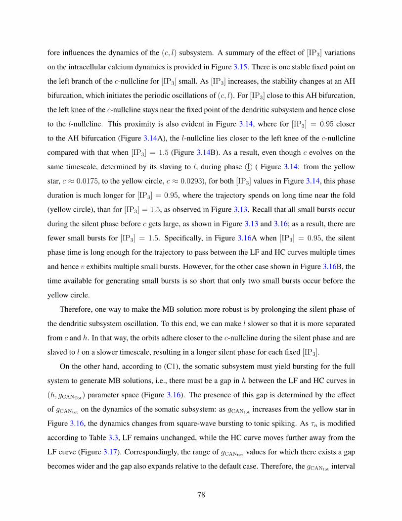
fore influences the dynamics of the (c, l) subsystem. A summary of the effect of [IP3] variations
on the intracellular calcium dynamics is provided in Figure 3.15. There is one stable fixed point on
the left branch of the c-nullcline for [IP3] small. As [IP3] increases, the stability changes at an AH
bifurcation, which initiates the periodic oscillations of (c, l). For [IP3] close to this AH bifurcation,
the left knee of the c-nullcline stays near the fixed point of the dendritic subsystem and hence close
to the l-nullcline. This proximity is also evident in Figure 3.14, where for [IP3] = 0.95 closer
to the AH bifurcation (Figure 3.14A), the l-nullcline lies closer to the left knee of the c-nullcline
compared with that when [IP3] = 1.5 (Figure 3.14B). As a result, even though c evolves on the
same timescale, determined by its slaving to l, during phase 1© ( Figure 3.14: from the yellow
star, c ≈ 0.0175, to the yellow circle, c ≈ 0.0293), for both [IP3] values in Figure 3.14, this phase
duration is much longer for [IP3] = 0.95, where the trajectory spends on long time near the fold
(yellow circle), than for [IP3] = 1.5, as observed in Figure 3.13. Recall that all small bursts occur
during the silent phase before c gets large, as shown in Figure 3.13 and 3.16; as a result, there are
fewer small bursts for [IP3] = 1.5. Specifically, in Figure 3.16A when [IP3] = 0.95, the silent
phase time is long enough for the trajectory to pass between the LF and HC curves multiple times
and hence v exhibits multiple small bursts. However, for the other case shown in Figure 3.16B, the
time available for generating small bursts is so short that only two small bursts occur before the
yellow circle.
Therefore, one way to make the MB solution more robust is by prolonging the silent phase of
the dendritic subsystem oscillation. To this end, we can make l slower so that it is more separated
from c and h. In that way, the orbits adhere closer to the c-nullcline during the silent phase and are
slaved to l on a slower timescale, resulting in a longer silent phase for each fixed [IP3].
On the other hand, according to (C1), the somatic subsystem must yield bursting for the full
system to generate MB solutions, i.e., there must be a gap in h between the LF and HC curves in
(h, gCANTot) parameter space (Figure 3.16). The presence of this gap is determined by the effect
of gCANtot on the dynamics of the somatic subsystem: as gCANtot increases from the yellow star in
Figure 3.16, the dynamics changes from square-wave bursting to tonic spiking. As τn is modified
according to Table 3.3, LF remains unchanged, while the HC curve moves further away from the
LF curve (Figure 3.17). Correspondingly, the range of gCANtot values for which there exists a gap
becomes wider and the gap also expands relative to the default case. Therefore, the gCANtot interval
78

0.02 0.04 0.06 0.080.4
0.5
0.6
0.7
0.8
0.9
c
l
(A)
0.02 0.04 0.06 0.080.4
0.5
0.6
0.7
0.8
0.9
c
l
(B)
Figure 3.14: Projection of the two MB solutions (black) from Figure 3.13 to (c, l)-space. The red
curve is part of the c-nullcline and the cyan curve is part of the l-nullcline. The yellow symbols
have the same meanings as in Figure 3.13. (A): [IP3] = 0.95. (B): [IP3] = 1.5. Other parameters
as in Figure 3.13.
over which bursting occurs in the somatic subsystem is broadened with the modified timescale for
n.
As a result, it is natural to expect that within the same amount of silent phase time of the den-
dritic subsystem oscillation, the mixed bursting model with the modified τn will be able to generate
more small bursts. This is not the case, however. In fact, for [IP3] = 1.5, the mixed bursting model
with the default τn yields an MB solution consisting of the same number of small bursts (Figure
3.17) as with the modified τn (Figure 3.16B). The effect of the adjustment of the timescale for
n is to increase the duration and the number of spikes within each small burst, corresponding to
the larger gap between the LF and HC curves, resulting in more biologically relevant small burst
events.
3.2.2 Robustness to gNaP
To study the robustness of MB solutions to gNaP, we fix [IP3] at 0.95. A systematic way to inves-
tigate the dependence of MB solutions on gNaP is via bifurcation analysis. Numerical simulations
show that as gNaP is increased, the behavior of the somatic subsystem switches from plateauing
79

0.6 1 1.4 1.80.4
0.6
0.8
1
[IP3]
l
PO
FPLK
Figure 3.15: Summary of how structures relevant to the activity of the dendritic subsystem de-
pend on the parameter [IP3], with all other parameters involved in the calcium dynamics as given
in Figure 3.13. The red solid (resp., dashed) curve indicates the l-coordinate of the stable (resp.,
unstable) intersection of the c- and l-nullclines, i.e., fixed points (FP), for the dendritic subsysys-
tem, while the blue curve denotes the l-coordinate of the left knee (LK) of the c-nullcline for the
dendritic subsystem, both parametrized by [IP3]. The two black vertical lines indicate the [IP3]
values of two AH bifurcations in the dendritic subsystem where the periodic oscillations (PO) of
(c, l) begin ([IP3] = 0.942602) and terminate ([IP3] = 1.58101), respectively.
to bursting to spiking, corresponding to the full system transitioning from bursting driven by the
dendritic subsystem (dendritic bursting [73, 47]) to mixed bursting to bursting that involves both
the somatic and dendritic subsystems but without a mix of burst types (somato-dendritic bursting
[73, 47]). A graphical summary of the effect of gNaP variations on the dynamics of the somatic sub-
system is provided in Figure 3.18, where the bifurcation structure of the somatic subsystem with
respect to gNaP for gCANTot= 0 is displayed. We plot gNaP against the standard Euclidean norm of
the solution. The plateauing branch of the somatic subsystem (red) is stable for the smaller gNaP
values. The stability changes at an AH bifurcation and the spiking family (blue) becomes stable at
a period doubling (PD) bifurcation. Moreover, the blue curve terminates at a homoclinic bifurca-
tion involving the unstable equilibrium branch (red). Between the spiking and the plateauing is the
80

0.3 0.35 0.4 0.45 0.5 0.55
0.02
0.03
0.04
0.05
h
gCANtot
(A)
0.3 0.35 0.4 0.45 0.5 0.55
0.02
0.03
0.04
0.05
h
gCANtot
(B)
Figure 3.16: The zoomed view of two-parameter bifurcation diagrams of HC (red), LF (blue)
and the trajectory (black) from Figure 3.13, projected into (h, gCANtot)-space. The yellow symbols
have the same meanings as in Figure 3.13. (A): [IP3] = 0.95, (B): [IP3] = 1.5. Other parameters
as in Figure 3.13.
0.35 0.4 0.45 0.5
0.02
0.03
0.04
0.05
0.06
h
gCAN
tot
LFHC (default)HC (modified)
Figure 3.17: Two curves of HC bifurcations (red solid, modified τn: σn = −5, an = 0.1; red
dashed, default τn: σn = −4, an = 0) and two overlapping curves of LF bifurcations (blue, default
and modified τn), in (h, gCANTot) parameter space. The black curve denotes the trajectory for the
default τn function, with other parameters the same as in Figure 3.13-3.16B. The yellow symbols
have the same meanings as in Figure 3.13.
81

0 2 4 6 8 10
40
45
50
55
60
AH
PD
Default
gNaP
L2Norm
(A)
0 2 4 6 8 10
40
45
50
55
60
AH
PD
gNaP
L2Norm
Modified
(B)
Figure 3.18: Effect of variations in gNaP on the behaviors of the somatic subsystem for(A) default
τn(v) and (B) modified τn(v) (denoted by the green curve in Figure 3.9A), respectively, with all
other parameters fixed at their standard values.
gNaP interval where the somatic subsystem is available in participating in bursting. According to
previous work on the square-wave burster [7], bursting patterns result for most of the gNaP interval
between the AH and PD bifurcations. Hence, as gNaP is increased, the transitions mentioned above
occur approximately at an AH bifurcation (onset of oscillations) and a PD bifurcation (transition
between bursting and spiking) for the somatic subsystem, respectively. Next we extend this bifur-
cation analysis and examine the dependence of MB solutions on both gNaP and gCANTot. To do this,
we compute two-parameter bifurcation diagrams in (gCANTot, gNaP)-space (Figure 3.19).
In Figure 3.19A, the somatic subsystem’s spiking/bursting boundary (blue, PD) was calculated
by following the PD point in (gCANTot, gNaP), while the boundary between bursts and plateau so-
lutions was computed by following the AH point where the fixed points of the somatic subsystem
lose stability. In panel (B), we show a similar a two-parameter bifurcation diagram for the modified
τn function. Comparing these two plots shows that for all gCANTotvalues below 0.05, i.e., for all
c values within a complete relaxation oscillation cycle, the somatic subsystem after modification
can generate bursting solutions for a wider range of gNaP. Recall that in order for the full system
to generate MB solutions, (C1) requires the somatic subsystem to engage in bursting for c values
arising during the silent phase of calcium. Hence with the new mix of timescales, MB solutions of
82

0 0.01 0.02 0.03 0.04 0.05
1
3
5
7
9
Default
gCANTot
gNaP
Spiking
Plateauing
Bursting
PDAH
(A)
0 0.01 0.02 0.03 0.04 0.05
1
3
5
7
9
Modified
gCANTot
gNaP
Plateauing
Bursting
SpikingPDAH(B)
Figure 3.19: Spiking/bursting and bursting/plateauing boundaries of the somatic subsystem for
(A) default τn(v) and (B) modified τn(v) as in Figure 3.18.
the mixed bursting model (3.4) become more robust to gNaP.
The bursting region for the somatic subsystem is broadened (Figure 3.19) due to the effect of
τn on its bifurcation diagram. As discussed in Section 3.2.1, for gNaP fixed, the bursting interval in
gCANtot becomes larger with the new τn function, since the range of gCANtot for which there exists
a gap in h between the LF and HC curves in (h, gCANtot)-space is increased. Similarly, for gCANtot
fixed, a gap between the LF and HC curves in (h, gNaP)-space is also required to obtain square-
wave bursting. Bifurcation analysis shows that this gap persists for a larger range of gNaP values
and therefore the bursting interval in gNaP becomes greater for the modified τn. Hence, the new
timescale for n helps enlarge the bursting region in (gCANtot , gNaP)-space, which in turn enhances
the robustness of MB solutions for the full system with respect to changes in gNaP for each fixed
gCAN.
3.3 DISCUSSION
We consider a single compartment reduction [47] of a two-compartment model of a pre-BotC
neuron [73], featuring both NaP and CAN currents, as well as intracellular calcium oscillations
83
that modulate the CAN current. Previous work characterized the regions of ([IP3],gNaP) parameter
space in which various types of solutions, namely somatic bursting, dendritic bursting, and somato-
dendritic bursting, occur in these models [73], [47]. While [47] presented a mathematical analysis
explaining relevant bursting mechanisms, based on the NaP current, the CAN current, or both
currents working together, less analysis about MB solutions was provided and little consideration
was given to identifying how many timescales are truly required to obtain these solutions or to
their robustness. In this Chapter, we have explained the mechanisms underlying MB solutions.
Our method is based on the ideas of fast-slow decomposition, implemented by considering the
interaction of two subsystems (one potentially bursting and the other intrinsically oscillating). This
approach is commonly used in the two timescale setting and has also recently been extended to a
three timescale system [41], as discussed in Chapter 2.
In the course of our analysis, we derive certain conditions on the timescales that together sup-
port MB solutions, based on which we obtain a non-intuitive result that the MB solution is in fact,
at its simplest, a two timescale phenomenon rather than requiring three timescales. Our analysis
about how to group timescales in this system may provide useful information for future studies of
irregular bursting solutions observed in other realistic biological models and in recordings from
respiratory CPG neurons as well as subthalamic nucleus (STN) neurons in the basal ganglia (e.g.
[3], [30], [14]). Our approach may also prove helpful to modelers making choices about timescale
groupings in other physical systems.
While parts of this work investigate rather specific details of the MB solution, we have also
followed our analysis with an investigation of how the mixed bursting model can be tuned to obtain
more robust MB solutions. In Section 3.2, we have investigated why the new mix of timescales that
we have found can support more robust MB solutions and hence have determined how to obtain a
larger MB region in ([IP3], gNaP) parameter space by changing timescales. Given that MB activity
is observed in pre-BotC recordings, we propose that the modified model that we have derived
would be a reasonable choice for incorporation in future studies of pre-BotC network dynamics.
From an MB state, both increases and decreases of gNaP that are sufficiently large should yield non-
mixed bursting. MB dynamics is predicted to be robust to slowing of IP3 dynamics but not with
respect to slowing of Ca2+ dynamics. Furthermore, although the contribution of a SNIC bifurcation
to MB dynamics is reminiscent of parabolic bursting [53], we nonetheless do not expect pre-BotC
84

neurons to exhibit behavior with the quantitative properties of parabolic bursting, because the fast
jumps in Ca2+, relative to the slower persistent sodium inactivation dynamics, will yield abrupt
transitions to rapid spiking and to quiescence (e.g., Figures 3.8A and 3.11E) even if there are two
fast subsystem SNIC events per cycle.
85

4.0 MULTIPLE TIMESCALE SIGH-LIKE BURSTING IN A SELF-COUPLED
PRE-BOTC NEURON
While our methods and analysis developed from Chapter 2 work well in revealing the mechanisms
underlying the mixed bursting (MB) solutions discovered in pre-BotC neurons in Chapter 3, we
have considered only one-directional coupling, from the dendritic to the somatic subsystem, such
that the mixed burst model can be thought of as one oscillator forcing another. Nonetheless, there
are many variations on the coupling among timescales that arise in other model systems. As noted
in Chapter 1, Jasinski et al. recently presented a more detailed model for neurons in the pre-BotC,
where each of membrane potential and cytoplasmic Ca2+ concentration can influence the evolution
of the other, and showed that a heterogeneous population of these neurons can generate sigh-like
bursting (SB) solutions that have similar MB solution patterns [30]. Furthermore, previous work
has suggested that the Na+/K+ pump, in addition to INaP and ICAN, plays an important role in the
generation of the MB solution, yet this is not considered in the system we have studied [56, 30].
Hence, in this Chapter, we focus on this more complicated model including additional multi-scale
forms of dynamics seen in respiratory neurons and synaptic coupling and exhibiting INaP, ICa,
Ca2+ oscillations, and the Na+/K+ pump current.
In contrast to previous mathematical models investigating the possible roles of INaP-dependent
and ICAN-dependent bursting mechanisms, in which these currents were included together in the
same model of single pre-BotC neurons [73, 47, 80], Jasinski et al. [30] mainly considered models
of heterogeneous neural populations. In fact, simulations in [30] showed that at the single-neuron
level, sigh-like bursting (SB) solutions no longer exist. Furthermore, the Na/K+ pump is needed to
generate the SB solution. Therefore, while the MB solution and the SB solution appear to be quite
similar (Figure 4.1), they may have very different bursting mechanisms. Besides understanding
the mathematical mechanisms, we are also interested in knowing whether the generation of SB
86

solutions requires the third timescale or not.
0 2000 4000 6000 8000
−50
−30
−10
10
Time(ms)
V
(A)
0 0.5 1 1.5 2
x 104
−60
−50
−40
−30
−20
Time(ms)
V
(B)
Figure 4.1: Mixed bursting solution (A) and sigh-like bursting solution (B) from [80] and [30],
respectively.
To facilitate the identification of the essential mechanisms underlying the SB behavior and the
assessment of how to group timescales, we consider a self-coupled model neuron based on the
network model presented in [30], which we refer to as the Jasinski model:
CdV
dt= −INa − INaP − IK − ICa − ICAN − IPump − IL − ISynE(4.1a)
dy
dt= (y∞(V )− y)/τy(V ), y = {mNa, hNa,mNap, hNap,mCa, hCa,mK}(4.1b)
ds
dt= ((1− s)s∞(V )− s)/τs(V )(4.1c)
dNai
dt= −αNa(INa + INaP + ICAN + 3Ipump)(4.1d)
dCatot
dt= −αCaICa − Cai/τCa(4.1e)
dCai
dt= −αCaICa − Cai/τCa + KCa(JERIN
− JEROUT)(4.1f)
dl
dt= AKd(1− l)− A[Ca]l(4.1g)
The conductance-based single-compartment model of a single neuron was developed in the
Hodgkin-Huxley style. The neuronal membrane potential (V ) is defined by a set of membrane
ionic currents, as shown in (4.1a). C is neuronal membrane capacitance and t is time. The ionic
87

currents in the model include fast Na+, persistent Na+, delayed rectifier K+, high-voltage-activated
Ca2+, Ca2+-activated nonspecific cation, Na+/K+ pump, leakage and excitatory synaptic currents
(see Table 4.1).
Table 4.1: Ionic currents and channel reversal potentials
Currents Reversal potentialsINa = gNa ·m3
Na · hNa · (V − ENa)ENa = (R · T/F ) · ln(Nao/Nai)INaP = gNaP ·mNaP · hNaP · (V − ENa)
IK = gK ·m4K · (V − EK) EK = (R · T/F ) · ln(Ko/Ki)
ICa = gCa ·mCa · hCa · (V − ECa) ECa = (R · T/2F ) · ln(Cao/Cai)ICAN = gCAN ·mCAN · (V − ECAN) ECAN = 0
IPump = RPump · (ϕ(Nai)− ϕ(Naieq)), where ϕ(x) = x3/(x3 +K3P)
IL = gL · (V − EL) EL = −68ISynE = (gSynE · s+ gtonic) · (V − ESynE) ESynE = −10
Activation (m) and inactivation (h) variables for most ionic channels are described as (4.1b),
where steady-state activation (m∞) and inactivation (h∞) and their time constants are described as
in Table 4.2. Notice from the bottom row in Table 4.2 that different from all other currents, ICAN
has instantaneous activation, which depends on Cai and is voltage-independent. The parameters
for these currents are specified in Table 4.3.
Table 4.2: Activation and inactivation variables
gating variables steady state activation and inactivation time constantsmNa
y∞(V ) = 1/(1 + exp(−(V − Vy1/2)/ky))τy(V ) = τymax/ cosh(−(V − Vτy1/2)/kτy)
hNa
mNaP
hNa
mCa τmCa= 0.5 ms
hCa τhCa = 18 ms
mKm∞ = α∞/(α∞ + β∞) τ∞ = 1/(α∞ + β∞)
α∞ = Aα · (V +Bα)/(1− exp(−(V +Bα)/kα)), β∞ = Aβ · exp(−(V +Bβ)/kβ)mCAN mCAN = 1/(1 + (KCAN/Cai)
n)
The intracellular concentration of free Ca2+ (Cai) is described by (4.1f), the right part of which
consists of four terms. The first two terms form the right hand side of the equation for the dynamics
of the total intracellular Ca2+ concentration within the cell (see (4.1e)), which differs from the
mixed bursting model in which Catot is assumed to be constant. The latter two terms are exactly
88

Table 4.3: Activation and inactivation variables
Current ParametersFast Na+ gNa = 150 nSINa Vm1/2 = −43.8 mV, km = 6 mV, τmmax = 0.25 ms,
Vτm1/2 = −43.8 mV, kτm = 14 mVVh1/2 = −67.5 mV, kh = −10.8 mV, τhmax = 8.46 ms,
Vτh1/2 = −67.5 mV, kτh = 12.8 mVPersistent gNaP = 0 nS
Na+ Vm1/2 = −47.1 mV, km = 3.1 mV, τmmax = 1 ms,Vτm1/2 = −47.1 mV, kτm = 6.2 mV
INaP Vh1/2 = −60 mV, kh = −9 mV, τhmax = 5000 ms,Vτh1/2 = −60 mV, kτh = 9 mV
In the case of non-inactivating INaP, h = constant = 0.4K+ delayed rectifier gK = 160 nS
IK Aα = 0.01, Bα = 44 mV, kα = 5 mV, Aβ = 0.17,Bβ = 49 mV, kβ = 40 mV
Ca2+ gCa = 0.00065 nSICa Vm1/2 = −27.5 mV, km = 5.7 mV, τm = 0.5 ms,
Vh1/2 = −52.4 mV, kh = −5.2 mV, τh = 18 ms
Ca2+-activated nonspecific ICAN gCAN = 3 nS,KCAN = 0.00074 mM, n = 0.97
Na+/K+pumpIpump Rpump = 200 pA,Naieq = 15 mM,Kp = 15 mM
Leakage IL gL = 2.5 nSExcitatory synaptic ISynE gSynE = 20 nS, gtonic = 0.78nS
the same as the right part of the equation for calcium in the mixed bursting model (compare (4.1f)
with (3.1d), so is the dynamics for l (compare (4.1g) with (3.1e)). Correspondingly, parameters
associated with JERin, JERout as specified in (3.2) and the equation for l are the same as given in
Table 3.1 in Chapter 3, except [IP3] = 1.5µM. For convenience, we henceforth omit units on the
parameter and variable values.
At the single-neuron level (when the self-coupling is removed by setting gSynE = 0), this
model can produce two types of intrinsic bursting behaviors, depending on chosen parameter val-
ues, similar to the mixed bursting model. One type of bursting (INaP-dependent bursting) is based
on the slow voltage-dependent inactivation of INaP (as represented by the hNaP variable in the
equation for INaP in Table 4.1), whereas the other type (ICAN-dependent bursting) relies on intra-
cellular Ca2+. Various distinct burst-terminating mechanisms based on the slow inactivation of
INaP, the activity-dependent accumulation of Na+ followed by the [Na+]in-activated IPump, and
the Ca2+-dependent inactivation of IP3R, respectively, exist this bursting neuron model.
89

In the presence of synaptic coupling between neurons (i.e., gSynE > 0), the coupled cells
are able to generate SB solutions. In this chapter, we consider the special case of a single self-
coupled cell model (4.1) as a reduction of coupled network. Numerical simulations show that
both mechanisms based on ICAN and IPump contribute to the generation of SB solutions, without
the need of INaP (e.g. SB solution dynamics will not be abolished at gNaP = 0, but will be lost
without CAN and Pump currents). The left panel of Figure 4.2 demonstrates one cycle of SB
solution patterns as well as changes in other relevant variables: Cai, Nai, Catot and l. Specifically,
there exist low-amplitude Cai and Nai transients during regular bursts followed by the jump up of
intracellular Ca2+, due to which Nai also exhibits high-amplitude transients. Besides, Catot and
l that are confined to the calcium subsystem (Cai,Catot, l) both accumulate until Cai jumps up.
After that, they start decreasing. The right panel of Figure 4.2 shows burst details that Cai, Nai
and Catot engage in small oscillations during the spiking phase of each regular burst since these
variables receiving input from V are perturbed by the voltage spike: they tend to increase as V
reaches its maximum and decrease as V oscillates to the minimum.
While the mixed bursting and Jasinski models generate similar solution patterns, the latter is
much more complicated than the former one in the sense that: first, (4.1) has one extra Na+/K+
pump-based burst-terminating mechanism, yet this is not considered in Chapter 3; second, instead
of one-directional coupling used in the mixed bursting model such that the model can be thought of
as one oscillator forcing another, membrane potential and cytoplasmic Ca2+ concentration in (4.1)
can each influence each other, so can membrane potential and intracellular Na+ concentration;
and third, in contrast to the model in Chapter 3, (4.1) incorporates and simulates more realistic
and detailed kinetics of the intracellular Ca2+ release. These complications and high dimension
of (4.1) (consisting of 13 variables) make the mathematical analysis of the Jasinski model quite
challenging.
One of the primary goals of this Chapter is to provide a thorough mathematical analysis of
the mechanisms underlying the SB solution. To this end, we will nondimensionalize to reveal
the presence of different timescales and identify how to group timescales in our model; implement
geometric singular perturbation theory to set up reduced systems based on separation of timescales;
and use the reduced systems to explain the mechanisms underlying the dynamics of SB solutions.
90

0 0.5 1 1.5 2
x 104
−60
−20
V
0 0.5 1 1.5 2
x 104
2
4
x 10−4
Cai
0 0.5 1 1.5 2
x 104
16
20
Nai
0 0.5 1 1.5 2
x 104
4
8x 10
−4
Catot
0 0.5 1 1.5 2
x 104
0.92
0.94
l
Time(ms)
6500 7000 7500 8000 8500−60
−40
−20
V
6500 7000 7500 8000 8500
1
2
3x 10
−5
Cai
6500 7000 7500 8000 8500
17
18
Nai
6500 7000 7500 8000 8500
5
5.5x 10
−4
Catot
6500 7000 7500 8000 8500
0.933
0.934
0.935
Time(ms)
l
Figure 4.2: Simulation of sigh-like rhythmic bursting of the Jasinski model. From top to bottom:
changes in membrane potential, calcium, sodium, total intracellular calcium concentration within
the cell (Catot) and IP3 channel gating variable l. This SB pattern repeats periodically. The right
panel shows the details of the regular small burst, where the dashed green and blue lines denote
the end and the beginning of the regular burst, respectively.
4.1 ANALYSIS OF SIGH-LIKE BURSTING
In this section, we analyze how various bursting mechanisms described above interact to produce
the SB solution, in the presence of self-excitation. As noted before, the SB solution dynamics will
not be abolished at gNaP = 0, i.e., INaP is not required in the Jasinski model for SB solutions. In
light of this, we can reduce (4.1) to a 11-dimensional system by removing mNaP and hNaP and
setting INaP = 0 in the equation (4.1a). Henceforth, we still refer to Jasinski model (4.1) as the
new lower dimensional model without involvement of INaP. Moreover, similar to the findings in
[30], numerical simulations of (4.1) indicate that the regular bursting is independent of ICAN as it
will not be abolished at gCAN = 0. However, assigning gCa = 0 or gCAN = 0 fully removes the
sigh-like oscillations, confirming that the generation of sigh-like bursts in this model is ICa/ICAN-
dependent. Similarly, setting IPump = 0 will lose both regular bursting and sigh-like oscillations,
91

implying that the Na+/K+ pump-based bursting mechanism is also involved. In conclusion, the
burst terminating mechanisms involved in the SB solution are depending on both Ca2+-dependent
IP3R inactivation and IPump activation. In the following, we aim to provide a mathematical anal-
ysis of how these two bursting mechanisms operate together to generate SB solutions.
The fact that both MB and SB solutions result from the interaction of two bursting mechanisms
highlights the possibility that analysis for understanding MB solutions may be carried over simi-
larly to the SB solution. Despite sharing one common burst terminating mechanism based on in-
tracellular Ca2+, these two solutions differ by the second operating burst-terminating mechanisms
that the MB solution is based on INaP inactivation, while the SB solution is IPump-based. In Chap-
ter 3, we analyzed the MB solution from a perspective of one potentially burster (depending on
INaP) driven by an intrinsically oscillating subsystem (Ca2+ oscillations). In the Jasinski model,
previous finding that regular burst depends on IPump while is independent of ICAN or ICa sug-
gests that we can decouple V, Nai from the calcium dynamics while regular bursting still persists.
Hence, we divide the Jasinski system into two subsystems: the system of equations (4.1a)-(4.1d)
(denoted as the voltage subsystem) as a potentially bursting subsystem and the system of equations
(4.1e)-(4.1g) (denoted as the calcium subsystem) as a potentially oscillating subsystem. With these
two subsystems, we adopt the approach used in Chapter 3 to explain the mechanisms underlying
the dynamics of the SB solution. We first investigate the IPump-based mechanism underlying the
regular burst generated by the voltage subsystem through a bifurcation analysis and then study the
effect of (Ca2+,Catot, l) subsystem on the resulting bifurcation structures to understand how the
transition from regular bursts to the long burst happens.
Our methods for analysis of the model will depend heavily on exploiting the presence of differ-
ent timescales. As a first step, it is helpful to rescale the variables so that the important timescales
can be explicitly identified. To this end, we nondimensionalize the model (details of the nondi-
mensionalization procedure are given in Appendix 6.4, with the timescales for all variables shown
in Table 6.1). While V , gating variables (mNa, hNa, mCa, hCa, mK) and s are not operating on the
same magnitude of timescales, it is clear that they are all relatively faster than others. Hence we
choose to group all of them as fast variables, Nai and Cai as slow, whereas l and Catot as evolving
on a superslow timescale. For simplicity, we abuse notation to let y ∈ R6 denote all the fast gating
variables and s. Using these information, we can now split our model into fast, slow and super-
92

slow subsystems. The procedure of setting up reduced systems is similar to what we have done in
Chapter 2 and hence is omitted here. The fast subsystem (V, y) consists of the equations for the fast
variables with both slow variables Cai and Nai treated as static parameters of the system. Since
changes in Catot and l affect the fast subsystem indirectly, they are not considered as parameters
for this subsystem. The Jasinski model (4.1) also has a two-dimensional slow subsystem consisting
of the equations for Cai and Nai with both superslow variables Catot and l fixed. Moreover, we
find it useful to work with the system consisting of all the fast and slow variables with superslow
variables fixed, which we denote as the fast-slow subsystem: (V, y,Cai,Nai).
As noted before, we will explain the mechanism from the perspective of how the IPump-based
burster is driven by the calcium subsystem. To do so, we first investigate the coupling effect be-
tween them. When decoupled from Ca2+ by setting gCa = gCAN = 0, the bifurcation diagram for
the (V, y,Nai) system is shown in Figure 4.3A, including an S-shaped curve equilibria (S) and a
family of stable periodic orbits (P) that initiates in a supercritical Andronov-Hopf (AH) bifurca-
tion and terminates in homoclinic (HC) bifurcation involving the middle branch of S. Hence, in the
absence of calcium dynamics, this subsystem is capable of generating a square-wave bursting so-
lution, the terminating mechanism of which is depending on the accumulation Nai and subsequent
activation of the Nai-dependent Na/K+ pump.
In the calcium subsystem (Cai,Catot, l), the dynamics of Ca2+ depends on the neuronal mem-
brane potential V . Hence, instead of exhibiting relaxation oscillations involving jumps in Cai be-
tween branches of the Cai-nullcline alternating with the drift in (Cai,Catot, l) along these branches,
there exist small oscillations during each regular burst (see Figure 4.3C and the trace for Cai in
Figure 4.2). Such patterns arise because the Cai-nullsurface moves back and forth between the
two surfaces as V oscillates between the minimum and maximum during the spiking phase of each
burst (Figure 4.3B and C). During the regular bursts, there is a low amplitude transient in Cai be-
fore it jumps up to the right branch, as noted before. Figure 4.3B shows that these two surfaces
corresponding to V at its minimum and maximum values lie close to each other due to the insen-
sitive dependence of ICa on V for calcium large. As a result, the trajectory bounded between the
two right branches is approximately evolving along the right branch of the Cai-nullsurface. Cai
decrease as l decreases until the trajectory jumps back to the left branch. What remains unclear
about this loop is to identify the bifurcation corresponding to the jump up of calcium, which should
93

10 20 30 40
−70
−50
−30
Nai
V
P (periodics)
S (equilibria)
AH
Nai-nullcline
HC(A) (B)
(C)
Figure 4.3: Basic structures of the voltage subsystem (4.1a)-(4.1d) and the calcium subsystem
(4.1e)-(4.1g). The first subsystem decouples from the calcium subsystem (Cai,Catot, l) by setting
gCa = gCAN = 0 . (A): Projection onto (Nai, V )-space of the bifurcation diagram for the first sub-
system along with the Nai-nullcline shown in cyan. The black solid (resp., dashed) curve S denotes
the stable (resp., unstable) fixed points of the Fast system with Nai taken as a constant parameter,
and the blue curve shows the maximum V along the family of periodics (P). (B): Nullsurfaces of
Cai for the calcium subsystem with V at their minimum (upper surface) and maximum (lower sur-
face), in (Cai,Catot, l)-space. The black curve denotes the SB solution trajectory of the Jasinski
model. The right branches of these two nullsurfaces lie close to each other. (C): An enlarged view
of (B). The trajectory jumps up to the right branch of the nullsurface of Cai near the red dot.
94
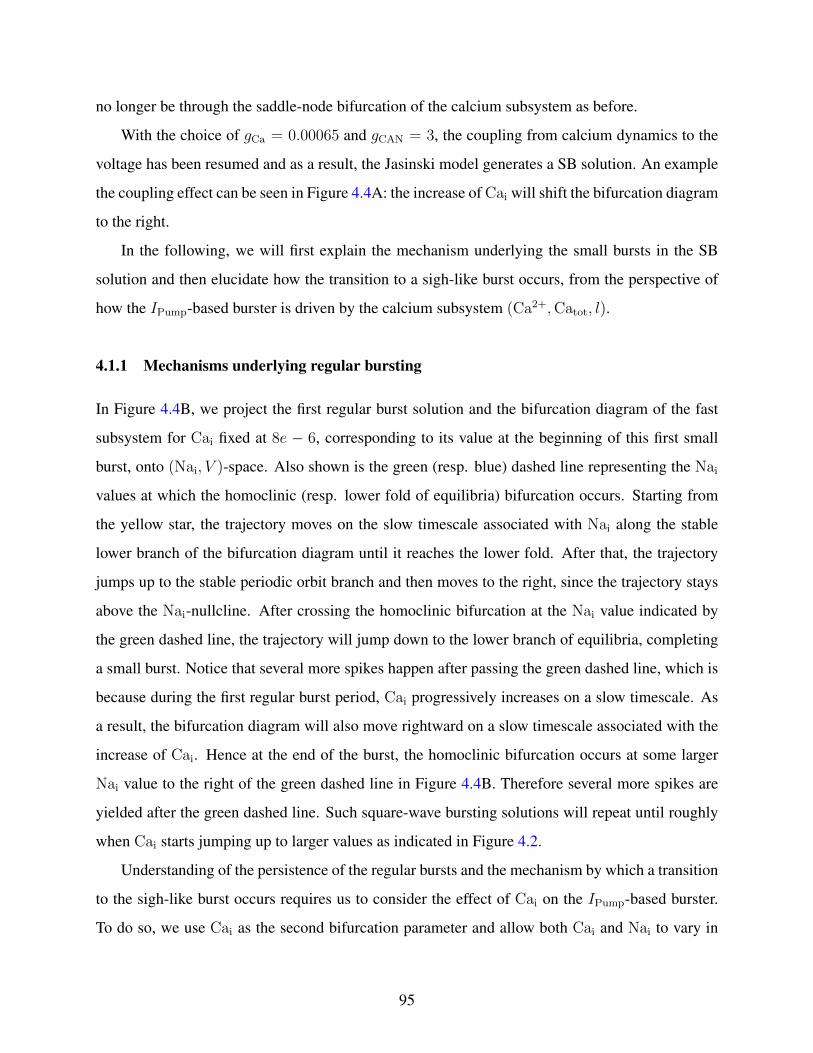
no longer be through the saddle-node bifurcation of the calcium subsystem as before.
With the choice of gCa = 0.00065 and gCAN = 3, the coupling from calcium dynamics to the
voltage has been resumed and as a result, the Jasinski model generates a SB solution. An example
the coupling effect can be seen in Figure 4.4A: the increase of Cai will shift the bifurcation diagram
to the right.
In the following, we will first explain the mechanism underlying the small bursts in the SB
solution and then elucidate how the transition to a sigh-like burst occurs, from the perspective of
how the IPump-based burster is driven by the calcium subsystem (Ca2+,Catot, l).
4.1.1 Mechanisms underlying regular bursting
In Figure 4.4B, we project the first regular burst solution and the bifurcation diagram of the fast
subsystem for Cai fixed at 8e − 6, corresponding to its value at the beginning of this first small
burst, onto (Nai, V )-space. Also shown is the green (resp. blue) dashed line representing the Nai
values at which the homoclinic (resp. lower fold of equilibria) bifurcation occurs. Starting from
the yellow star, the trajectory moves on the slow timescale associated with Nai along the stable
lower branch of the bifurcation diagram until it reaches the lower fold. After that, the trajectory
jumps up to the stable periodic orbit branch and then moves to the right, since the trajectory stays
above the Nai-nullcline. After crossing the homoclinic bifurcation at the Nai value indicated by
the green dashed line, the trajectory will jump down to the lower branch of equilibria, completing
a small burst. Notice that several more spikes happen after passing the green dashed line, which is
because during the first regular burst period, Cai progressively increases on a slow timescale. As
a result, the bifurcation diagram will also move rightward on a slow timescale associated with the
increase of Cai. Hence at the end of the burst, the homoclinic bifurcation occurs at some larger
Nai value to the right of the green dashed line in Figure 4.4B. Therefore several more spikes are
yielded after the green dashed line. Such square-wave bursting solutions will repeat until roughly
when Cai starts jumping up to larger values as indicated in Figure 4.2.
Understanding of the persistence of the regular bursts and the mechanism by which a transition
to the sigh-like burst occurs requires us to consider the effect of Cai on the IPump-based burster.
To do so, we use Cai as the second bifurcation parameter and allow both Cai and Nai to vary in
95

15 16 17 18 19 20 21
−60
−20
20
Nai
V
[Ca] = 8e − 6 3e − 5 5e − 5
(A)
15 16 17 18 19 20
−60
−40
−20
Nai
V
(B)
17 18 19 20
2
4
6
8x 10
−5
LF
HC
Nai
Cai
Active
Silent
(C)
Figure 4.4: Bifurcation diagrams of the Fast system (4.1a)-(4.1c) with the slow variables Nai and
Cai taken as static parameters. The yellow symbol marks the start point of the SB solution. (A):
The effect of Cai on the bifurcation diagram for the Fast system, projected into (Nai, V )-space,
along with the Nai-nullcline (cyan). Increasing Cai from 8e−6 to 3e−5 to 5e−5 results in a shift
of the bifurcation diagram to the right (black to blue to green). (B): Projection of the first small
burst in the SB solution from (A) onto the bifurcation diagram (with Cai = 8e − 6) in (Nai, l)-
space, along with the Nai-nullcline (cyan). The blue and green dashed lines indicate the Nai values
where the lower fold and homoclinic bifurcations occur, respectively. (C): The curve of saddle-
node bifurcations corresponding to the lower fold of the bifurcation diagram (blue), homoclinic
bifurcation curve (green) and part of the trajectory (black) from (A) in (Nai,Cai)-space. The green
curve acts as the boundary of the oscillation region for the Fast system.
96

order to find the two-parameter bifurcation curves of the fast subsystem (V, y) in the (Nai,Cai)
parameter plane that unify the results in Figure 4.4A, as illustrated in Figure 4.4C. The blue (resp.
green) curve in this plane is the curve of lower fold (LF) (resp. homoclinic (HC)) bifurcations,
which initiates (resp. terminates) each burst, as noted previously. Since the increase of Cai moves
the bifurcation diagram to the direction of increasing Nai, both curves of LF and HC are positively
sloped in the (Nai,Cai)-space. Within the same projection, the trajectory evolves leftward from the
yellow star and it starts oscillating as it passes the LF curve (see Figure 4.4C). These oscillations
terminate when the trajectory reaches the HC bifurcation curve, which completes the first regular
burst. Similarly, a sequence of subsequent regular bursts occurs, with the local maximum of Nai
progressively increasing due to the right drift of LF as Cai accumulates. The fact that the trajectory
in (Nai,Cai)-space crosses the LF and HC 15 times corresponds to the existence of the 15 regular
bursts (see Figure 4.2). After that, bursting solutions give way to continuous spiking.
Based on the fast subsystem bifurcation structures in this section, we demonstrate that regular
bursts occur as the slow variables Cai and Nai traverse the phase space back and forth between the
LF and HC curves. The reason why regular bursts switch to the sigh-like burst, however, remain
unknown. To figure this out, we notice that after multiple crossings with the HC curve in Figure
4.4C, the trajectory projected to (Nai,Cai) space starts oscillating near the HC curve, instead of
going back to quiescence state. Moreover, this transition happens before Cai jumps up. Hence, the
switch from regular bursts to the long burst in the full system seems to correspond to the transition
from bursting to tonic spiking in the fast-slow subsystem (V, y,Nai,Cai), rather than the jumping
up of Cai as in the mixed bursting model.
4.1.2 Mechanisms underlying the transition from regular bursts to the sigh-like burst
In the analysis up to this point, superslow variables have not been considered yet. It is natural
to expect that the superslow evolution of these two variables may contribute to the switch from
bursting to the tonic spiking. A numerical simulation of the fast-slow subsystem over a range
of Catot and l values (Figure 4.5) suggests that superslow variables do play an important role in
inducing a transition from bursting to tonic spiking in the fast-slow subsystem. In Figure 4.5 (top
panel), representative time traces for bursting and tonic spiking solutions are shown for a fixed
97

value of l. For small Catot, the fast-slow system is in a bursting state (Figure 4.5, top left). When
Catot is increased, tonic spiking solutions arise (Figure 4.5, top middle). A further increase in
Catot does not change the tonic spiking in V (Figure 4.5, top right), but both Cai and Nai oscillate
at higher values than in (A) and (B) . A graphical summary of the effect of Catot variations on
the trajectories is provided in panel (D), where the bifurcation structure of the fast-slow subsystem
with respect to Catot for l = 0.94 was computed. We plot Catot against the standard Euclidean
norm of the solution. As Catot is increased, the behavior switches from bursting to tonic spiking.
The fast-slow system exhibits tristability between the bursting (red solid) and tonic spiking (blue
solid) for the small Catot values. Both branches become unstable at saddle-node bifurcations. The
initial conditions are chosen such that the trajectory will be attracted by the stable bursting branch
for Catot = 00006 (red diamond). As the tristability is lost for bigger Catot values (e.g., 0.0007 and
0.00074 denoted by the blue diamonds on the upper and lower branches of the spiking solutions,
respectively), the behavior switches to tonic spiking. Note that the lower L2 norm corresponds to
larger Cai and Nai values, hence as the trajectory gets attracted by the lower branch of spiking
after the saddle node bifurcation, the tonic spiking solution occurs at larger Cai, Nai values.
To understand the mechanisms underlying the switch from bursting to tonic spiking, we use
slow averaged dynamics in the oscillation (bursting or spiking) region to analyze activity states.
For convenience, we refer to the two regions of (Nai,Cai) space separated by the curve of HC
bifurcations which terminates each burst as the silent and active regions (Figure 4.4C).
During the interburst interval of the regular burst cycle, the full model dynamically collapses
to a lower-order system governed by the slow variables Cai and Nai restricted to the manifold of
equilibrium points of the fast subsystem. This interburst interval corresponds to the silent region
of (Nai,Cai) space. During the spiking phase of each regular burst, the solution trajectory is still
largely determined by the slow variables Cai and Nai, but these variables are perturbed by the volt-
age spike and Ca2+-influx associated with each action potential. This spiking phase corresponds
to the active region of (Nai,Cai) space. In this region we employ the method of average nullclines,
a numerical technique in which the derivatives of the slow variables are averaged over one cycle of
the action potential, while the superslow variables Catot and l are treated as the static parameters.
By doing so, we reduce the fast-slow subsystem to two equations for just the slow variables. For
g1 and g2 defined as the right hand sides of (4.1f) and (4.1d), respectively, the reduced system can
98

2000 3000 4000 5000
−60
−50
−40
−30
−20
Time (ms)
V
4 4.1 4.2 4.3
x 104
−60
−50
−40
−30
−20
V
Time (ms)4 4.1 4.2 4.3
x 104
−60
−50
−40
−30
−20
Time (ms)
V
6 6.5 7
x 10−4
51
52
53
54
Catot
L2−
NORM
l = 0.94
Bursting
Tonic Spiking
Figure 4.5: Effect of variations in Catot on the trajectories of the fast-slow subsystem
(V, y,Cai,Nai) for l = 0.94. Top row, from left to right: Catot = 0.0006 (bursting), Catot =
0.0007 (tonic spiking at low Cai and Nai: Cai ≈ 2.5 × 10⁻⁵,Nai ≈ 18) and Catot = 0.00074
(tonic spiking at high Cai and Nai: Cai ≈ 5.7 × 10⁻⁴ and Nai ≈ 25.5). The bifurcation diagram
for the fast-slow subsystem with respect to the Catot in the bottom row summaries all possible
behaviours as Catot varies: bursting (red curves) and tonic spiking (blue curves) in which solid
means stable, while dashed means unstable. The three diamonds from top to bottom indicate Catot
values used by the top three panels from left to right, respectively.
be written as
< Cai > =1
T (Cai,Nai)
∫ T (Cai,Nai)
0
g1(V (Cai,Nai; t),Cai,Catot, l),(4.2a)
< Nai > =1
T (Cai,Nai)
∫ T (Cai,Nai)
0
g2(V (Cai,Nai; t),Cai,Catot, l)(4.2b)
99

We refer to the reduced problem (4.2) as the averaged slow system. The average Nai and
Cai nullclines are steady-state periodic solutions (with period T ) of the fast-slow subsystem along
with the additional constraint of either < Cai >= 0 or < Nai >= 0. In future discussions of
the dynamics of the averaged slow system, we will refer to the Cai and Nai average nullclines as
Caav and Naav, respectively. The intersection of Caav and Naav, a quasi-steady-state fixed point
representing a tonic spiking solution, will be referred to as Fav.
Figure 4.6 illustrates phase planes of the average slow system (4.2) for l = 0.94 and Catot =
0.0006, 0.0007, 0.00074 as in Figure 4.5. In each panel of Figure 4.6, the green curve represents
the HC bifurcation of the fast subsystem, the boundary of the oscillation region. When a bursting
solution crosses HC, it falls back to the silent phase, and spiking activity stops until a subsequent
burst cycle begins (Figure 4.4C). Above HC, averaged nullclines Caav (blue curve) and Naav
(green curve) are shown. As noted before, fixed points of (4.2), Feq (yellow diamond), are given
by the intersections of these nullclines, and one can usually determine the stability of the fixed
points by considering the nullcline configuration.
In Figure 4.6A when Catot = 0.0006, the two average nullclines intersect at a stable fixed point
Fav1 (yellow diamond), which corresponds to the upper spiking branch in Figure 4.5 (bottom).
Despite the existence of stable fixed point (corresponding to stable tonic spiking), the fast-slow
subsystem exhibits bursting since our chosen initial values lie in the basin of attraction of the
bursting branch. For Catot = 0.0007, the stability of bursting is lost and hence the trajectory is
now attracted by Fav1 (Figure 4.6B, yellow diamond). Besides the saddle node Fav2 in the middle,
the third fixed point of (4.2) that lies in larger Cai and Nai values corresponding to the lower spiking
branch in Figure 4.5 (bottom) is not visible here. As a result, the fast-slow subsystem converging
to the lower stable fixed point Fav1 exhibits tonic spiking. As Catot increases further to 0.00074,
the lower two fixed points Fav1 and Fav2 collide and annihilate each other through a saddle-node
bifurcation (Figure 4.6C) and we are only left with the upper stable fixed point Fav3 (Figure 4.6D,
yellow diamond), which corresponds to the lower spiking branch in Figure 4.5 (bottom) as noted
before. Therefore, the trajectory jumps up to large Cai value on the slow timescale until reaching
the average Cai nullcline (blue curve). Once there, the trajectory starts moving rightward to the
fixed point Fav3 since < Cai > is nearly 0 while < Nai > remains positive. As the trajectory
eventually arrives at Fav3, a tonic spiking solution results at large Cai and Nai values.
100
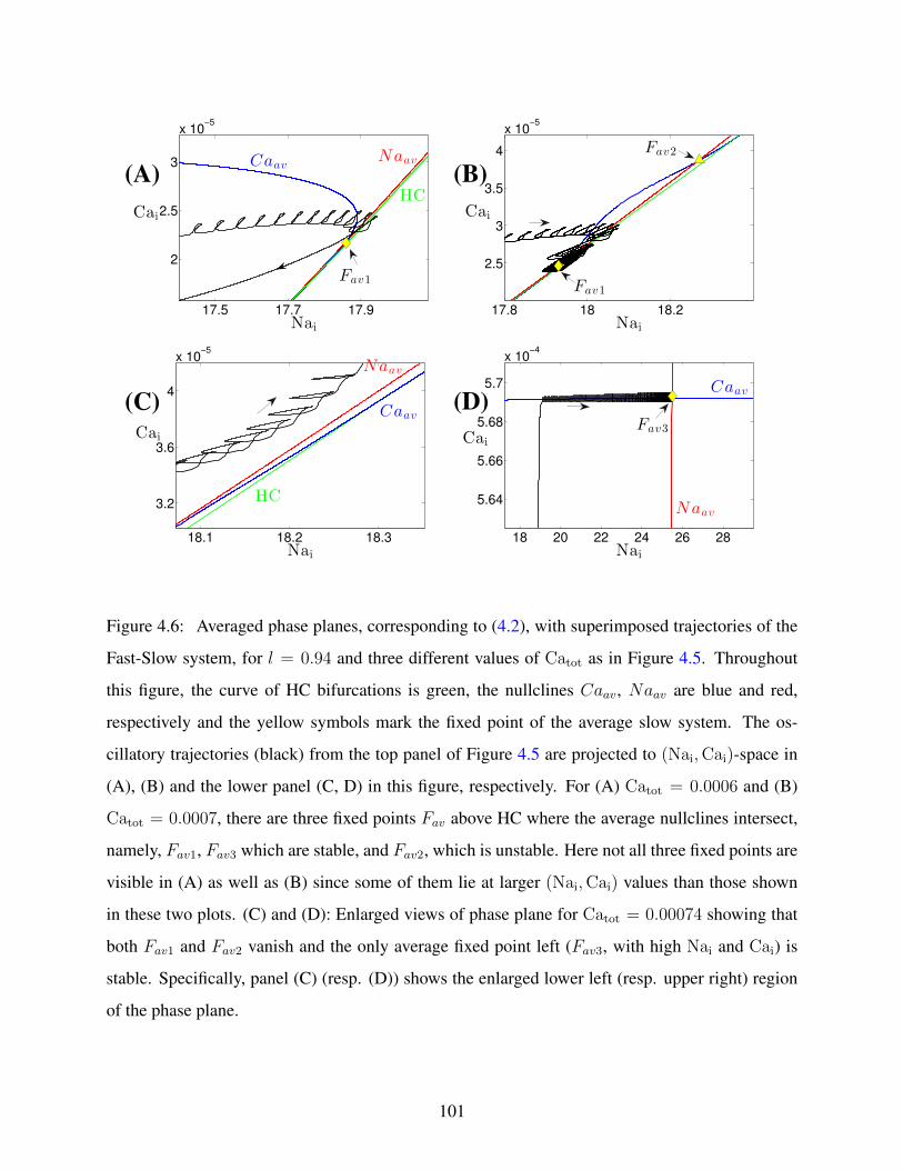
17.5 17.7 17.9
2
2.5
3
x 10−5
CaavNaav
HC
Nai
Cai
Fav1
(A)
17.8 18 18.2
2.5
3
3.5
4
x 10−5
Nai
Cai
Fav1
Fav2
(B)
18.1 18.2 18.3
3.2
3.6
4
x 10−5
Nai
Cai
Caav
Naav
HC
(C)
18 20 22 24 26 28
5.64
5.66
5.68
5.7
x 10−4
Nai
Cai
Fav3
Naav
Caav(D)
Figure 4.6: Averaged phase planes, corresponding to (4.2), with superimposed trajectories of the
Fast-Slow system, for l = 0.94 and three different values of Catot as in Figure 4.5. Throughout
this figure, the curve of HC bifurcations is green, the nullclines Caav, Naav are blue and red,
respectively and the yellow symbols mark the fixed point of the average slow system. The os-
cillatory trajectories (black) from the top panel of Figure 4.5 are projected to (Nai,Cai)-space in
(A), (B) and the lower panel (C, D) in this figure, respectively. For (A) Catot = 0.0006 and (B)
Catot = 0.0007, there are three fixed points Fav above HC where the average nullclines intersect,
namely, Fav1, Fav3 which are stable, and Fav2, which is unstable. Here not all three fixed points are
visible in (A) as well as (B) since some of them lie at larger (Nai,Cai) values than those shown
in these two plots. (C) and (D): Enlarged views of phase plane for Catot = 0.00074 showing that
both Fav1 and Fav2 vanish and the only average fixed point left (Fav3, with high Nai and Cai) is
stable. Specifically, panel (C) (resp. (D)) shows the enlarged lower left (resp. upper right) region
of the phase plane.
101

Using slow averaged dynamics, we have elucidated how the transition from bursting to tonic
spiking occurs and why Cai jump ups to larger values as Catot increase for l fixed. Similarly,
we summarize the effects of Catot on the average slow system by using bifurcation analysis as
shown in Figure 4.7. Again, the upper (resp. lower) branch of the bifurcation diagram in L2
norm corresponds to the lower (resp. upper) branch in Cai as well as Nai and hence solutions in
this branch denote Fav1 (resp. Fav3). The middle branch represents the unstable saddle Fav2 (see
Figure 4.6B). Notice that Figure 4.7 looks qualitatively the same as the tonic spiking branch shown
by the blue curve in Figure 4.5 (bottom), hence both can be used to illustrate the influence of Catot
on the oscillatory trajectories for fixed value of l. As Catot is increased, calcium jumps up at a
saddle-node (SN) of either the tonic spiking branch in Figure 4.5 (bottom) or the branch of average
fixed points in Figure 4.7. On the other hand, the onset of spiking happens at a SN of the bursting
branch (Figure 4.5 (bottom), red curve). Next we extend this bifurcation analysis and examine the
dependence of the solution patterns of the fast-slow system on both Catot and l. To do this, we
compute two-parameter bifurcation diagrams in (Catot, l)-space.
0 2 4 6 8
x 10−4
42
44
46
48
50
Catot
L2−
NORM
l = 0.94
Fav1
Fav2
Fav3
Figure 4.7: Bifurcation diagram of the average slow system (4.2) with respect to Catot with
l fixed at 0.94. The Catot values for the blue diamond marker points from upper to lower are
Catot = 0.0007 (as in Figure 4.6B) and 0.00074 (as in Figure 4.6C, D), respectively.
In Figure 4.8C, the spiking/bursting boundary (solid red, SN1) was calculated by following
in 2 parameters the SN point where the bursting branch loses stability (Figure 4.5 (bottom), the
SN of the red curve). Also shown is the boundary (solid blue, SN2) denoting the onset of jump-
102

ing up of Cai (also computed by following in (Catot, l) the upper fold point of the tonic spiking
branch in Figure 4.5 (bottom)). We can also use direct simulation of the fast-slow subsystem (e.g.,
fixing Catot, varying l systematically, and then repeating for a different Catot), to estimate the
bursting/spiking boundary curve and the onset of the jump up in calcium (shown in dashed red
and blue). The distance between the solid red (resp. blue) and the dashed red (resp. blue) will
be shortened as we exaggerate the timescale separation between the fast-slow subsystem and the
superslow variables.
Together with fast subsystem bifurcation structures as illustrated in Figure 4.4B, and repro-
duced in Figure 4.8B, we are now able to fully understand the SB solution. Starting from the
yellow star at low Catot and l (Figure 4.8C), a sequence of small bursts is produced as the trajec-
tory in (Cai,Nai)-space reaches the LF and HC curves multiple times (Figure 4.8B). This process
should be terminated as the increases of Catot and l push the trajectory in (Catot, l)-space across
the SN1, entering the tonic spiking regime, as we discussed before. Nonetheless, several more
small bursts actually occur after passing the SN1 and are followed by the start of tonic spiking at
the triangle. In the singular limit, however, this additional bursting will be lost and the tonic spik-
ing occurs after passing SN1. In (Catot, l)-space, the trajectory evolves rightward from the triangle
and eventually passes the SN2 curve at some point close to the yellow circle which initiates the
jump up of Cai (Figure 4.8C). The slow increase in Cai as well as in Nai can be seen in panel
(B) showing the trajectory in (Nai,Cai)-space jumps to the upper right from the yellow circle,
corresponding to the trajectory projected into (Cai,Catot, l)-space converging to the right branch
of the Cai-nullsurface and reaching the maximum of Cai (Figure 4.3B). For Cai big, the trajectory
in (Cai,Catot, l)-space is bounded by two nearly overlapping surfaces (see Figure 4.3B) and lies
above the l-nullsurface (not shown here), consequently, l will decrease, leading to the reduction
of Cai. Therefore, the trajectory in (Nai,Cai)-space falls back from the peak in Cai direction and
moves towards HC. Once crossing the HC bifurcation curve at the yellow square, the long burst
will be terminated and the trajectory enters the silent phase. As the solution finally returns to the
starting point, one cycle of the SB solution is completed.
Remark 4. Just as the MB solution, after Cai jumps up at the yellow circle, there exists a sudden
decrease in the amplitude of the V spikes, followed by spikes with incrementing amplitudes (Figure
4.8A). This feature arises because the voltage subsystem in the Jasinski model share a similar
103

0 0.5 1 1.5 2
x 104
−60
−50
−40
−30
−20
Time(ms)
V
(A)
16 17 18 19 20 21
1
3
5
x 10−4
Nai
Cai
LFHC
(B)
4 5 6 7
x 10−4
0.93
0.94
Catot
l
SN1SN2
(C)
Figure 4.8: Simulation of the SB solution generated by the Jasinski model (4.1), together with
the bifurcation diagrams. (A): Temporal evolution of V . (B): Two parameter bifurcation dia-
grams showing LF (blue) and HC (green) curves together with the trajectory from panel (A) in
(Nai,Cai)-space, the enlarged view of the lower left part of which is given by Figure 4.4C. (C):
The curves of saddle-node bifurcations corresponding to the upper folds of the bursting branch
and the spiking branch in Figure 4.5 (bottom), respectively. We use SN1 (solid red) to approximate
the bursting/spiking boundary (dashed red) and use SN2 (solid blue) to approximate the onset of
jumping up of Cai (dashed blue), respectively.
104

bifurcation structure: periodic orbit amplitudes initiate small at the AH bifurcation and increase as
Nai gets closer to the HC bifurcation (Figure 4.3A). This is qualitatively similar to the bifurcation
structure of the somatic subsystem in Chapter 3. Hence following the same argument as discussed
in Chapter 3, the amplitude of spikes near the end of the sigh-like burst is increasing.
4.2 IDENTIFYING TIMESCALES
We obtain a non-intuitive result in Chapter 3 that genesis of MB solution does not require a third
timescale, a natural question would be: how many timescales are involved in the SB solution?
These two solutions appear to be quite similar based on their time courses, yet the underlying
mechanisms are different. Moreover, through our analysis on the SB solution in Section 4.1, both
slow and superslow variables seem to play important roles in determining generation of regular
bursting and the transition to the last long burst. To figure this out, we adopt the approach used in
Section 2.3 by transforming our original system into certain two-time-scale systems by adjusting
system parameters (see Table 6.1 in Appendix 6.4). Then we consider whether these systems can
generate solutions that are similar to SB solution considered in this Chapter. Firstly, we choose
A = 1 so that l evolves on a comparable timescale as Catot. Since parameters that control the
timescale for Cai will also affect the timescale for Catot, we introduce a new parameter, β, with
default value 1, as the scaling factor for right hand side of (4.1f), such that we can increase or
decrease β to make Cai faster or slower. To change the timescale for Nai, we vary αNa. Originally
the Jasinski model has 7 fast, 2 slow, and 2 superslow (7F, 2S, 2SS) variables. As noted before,
there are many ways to regroup these timescales to be a two-time-scale system. Here we speed
up Cai and Nai by increasing both β and αNa by a factor of 100 to produce a system with 9 fast
and 2 superslow (9F, 2SS) variables. Another rescaling that we choose to use is slowing the two
slow variables by reducing both β and αNa by a factor of 10, respectively, to constitute a (7F,
4SS)-system.
With original scaling, (4.1) generates a SB solution, as shown in Figure 4.2. The modification
on the timescale of l does not change this solution qualitatively, except the number of small bursts is
less. This is because as l becomes faster, the trajectory projected into (Catot, l)-space will reach the
105

spiking/bursting boundary curve (SN1) earlier and hence small bursts transit to long burst earlier
(Figure 4.8C). We first compare the SB solution to solutions from the (9F, 2SS) version of the
system (4.1) described above (compare Figure 4.2 with Figure 4.9A). The fast/slow decomposition
method (between (V, y) and Nai, Cai) for understanding the mechanisms underlying the regular
bursts within the SB solution no longer applies to the (9F, 2SS) case, because Cai and Nai are now
evolving fast. In contrast to the original (7F, 2S, 2SS) case where the (7F, 2S)-subsystem generates
bursting solutions for relatively small Catot and l values (see Figure 4.5 and 4.8C), the new 9-
dimensional fast subsystem for (9F, 2SS) case exhibits tonic spiking for all Catot and l values
within a complete bursting cycle. A graphical summary of the effect of Catot on the trajectories
is provided in panel (B), where the bifurcation diagram of the fast subsystem (9F) with respect to
Catot for l = 0.94 was computed. The tonic spiking solutions persist for all Catot values, while
bursting branch that was found in the original system no longer exists in this case. Therefore, the
spiking persists throughout the full period, failing to yield a SB solution.
Under the alternative rescaling to a (7F, 4SS) system, the bursting solution is as shown in Figure
4.10A. The square-wave bursting properties have been restored, In fact, the (7F, 2S, 2SS) and (7F,
4SS) systems have the same fast subsystem with all other slow/superslow variables fixed. Similar
bifurcation analysis of this fast subsystem as illustrated before can be used to explain the bursting
solution in this rescaled system (see Figure 4.10B). Within the projection into the (Nai,Cai)-space,
the oscillations begin as the trajectory reaches the LF curve, where it turns around and evolves
rightward. Notice that Cai and Nai are now evolving on a superslow timescale, the drift of the
trajectory in the direction of increasing Cai and Nai after passing the curve of LF bifurcations is
too slow for the solution to reach the curve of HC bifurcations. As a result, bursting continue
until the transition to tonic spiking (due to the increase of Catot and l) happens. While oscillations
continue, all four superslow variables are increasing superslowly and eventually Cai jumps up to a
relatively larger value, from which Cai starts decreasing (Figure 4.10C). Again similarly as before,
this reduction in Cai is fundamental in terminating the burst as it brings the trajectory across the
curve of HC bifurcations. Afterwards, the solution enters the silent phase and goes back to the
starting point, completing one cycle of one single long burst. The mechanisms underlying the
switch from bursting to tonic spiking and the onset of the jump up of calcium can be understood
using a similar averaging method as used in Section 4.1.2 and hence details are omitted here.
106
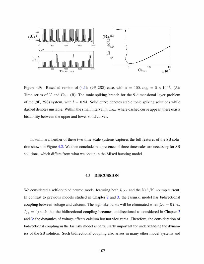
0 500 1000 1500 2000
−50
−30
V
0 500 1000 1500 20000
1
2
x 10−4
Cai
Time (ms)
(A)
5 10 15
x 10−4
51
52
53
Catot
L2−
NORM
(B)
Figure 4.9: Rescaled version of (4.1): (9F, 2SS) case, with β = 100, αNa = 5 × 10⁻³. (A):
Time series of V and Cai. (B): The tonic spiking branch for the 9-dimensional layer problem
of the (9F, 2SS) system, with l = 0.94. Solid curve denotes stable tonic spiking solutions while
dashed denotes unstable. Within the small interval in Catot where dashed curve appear, there exists
bistability between the upper and lower solid curves.
In summary, neither of these two-time-scale systems captures the full features of the SB solu-
tion shown in Figure 4.2. We then conclude that presence of three timescales are necessary for SB
solutions, which differs from what we obtain in the Mixed bursting model.
4.3 DISCUSSION
We considered a self-coupled neuron model featuring both ICAN and the Na+/K+-pump current.
In contrast to previous models studied in Chapter 2 and 3, the Jasinski model has bidirectional
coupling between voltage and calcium. The sigh-like bursts will be eliminated when gCa = 0 (i.e.,
ICa = 0) such that the bidirectional coupling becomes unidirectional as considered in Chapter 2
and 3: the dynamics of voltage affects calcium but not vice versa. Therefore, the consideration of
bidirectional coupling in the Jasinski model is particularly important for understanding the dynam-
ics of the SB solution. Such bidirectional coupling also arises in many other model systems and
107

0 0.5 1 1.5 2 2.5 3 3.5 4
x 104
−70
−60
−50
−40
−30
−20
V
0 0.5 1 1.5 2 2.5 3 3.5 4
x 104
0
1
2
x 10−4
Cai
Time (ms)
(A)
16.5 17 17.5 18 18.5 19 19.5
2
6
10
14
18
x 10−5
LF
HC
Nai
Cai
(B)
(C)
Figure 4.10: Rescaled version of (4.1): (7F, 4SS) case, with β = 0.1, αNa = 5× 10⁻⁶. (A): Time
series of V and Cai. (B): The projection of the trajectory from (A) onto the two parameter bifur-
cation diagram for the 7-dimensional layer problem of the (7F, 4SS) system. (C) Cai-nullsurfaces
and trajectory (black) are the same as illustrated in Figure 4.3B and C, together with the trajectory
(magenta) of the (7F, 4SS) system from (A).
108

is more biologically relevant. In this Chapter, we have extended and applied methods and analysis
from previous chapters to the Jasinski model and explained the mechanisms underlying the SB
solution. While the bidirectional coupling between V and Cai as well as more detailed Ca2+ dy-
namics make the implementation of the decomposition method more difficult, we applied fast-slow
averaging to help explain the mysterious parts which cannot be done using the approach in Chapter
3 for MB solution. Besides describing specific details of SB solution features, we have also in-
vestigated whether this solution is truly three timescale phenomena or not. Different from the MB
solution, our analysis shows that SB solution features are lost under grouping to two timescales
and hence can be said to require at least three timescales.
As in Chapter 3, several conditions for supporting the SB solution can also be implied from
our analysis in this Chapter. In order to obtain SB solutions, we require relatively small gCa since
large gCa will remove SB patterns in the Jasinski model. Notice that the increase of gCa will speed
up Cai (see Table 6.1) such that the time allowing for generating small bursts becomes shorter and
as a result, the number of small bursts decreases. If we keep increasing gCa, the small bursts will
completely disappear and the SB solution will be lost. This suggests that it is necessary that the V
subsystem acts as a square-wave burster for Cai values arising during regular bursts, so that there
exist small burst solutions before Cai jumps up to its active phase. Second, the time before Cai
jumps up should be long enough to allow for multiple crossings between the LF and HC curves
in the (Nai,Cai)-space. As suggested by the (9F, 2SS) case shown in Figure 4.9, each crossing
between the LF and HC should be slow enough for the full system to generate bursts instead of
tonic spiking solutions. More rigorous analysis on what conditions on the timescales that together
support SB solutions will need to be done in the future, which may provide useful information for
building minimum model for SB solutions as well as how can we make the solution more robust
by tuning the model, as we did Chapter 3.
Another future work is to understand why the self-excitation plays such an essential role that
without it, SB solution no longer exists. In our setting, we have chosen gSynE = 20 to obtain the SB
solutions. Decrease of gSynE will eliminate the SB dynamics, which agrees with the findings from
[30] that the SB is an emergent, network interaction-dependent bursting solution. A numerical
simulation shows that decrease of gSynE will result in a transition from bursting to spiking in the
voltage subsystem. Hence, for gSynE small such that the voltage subsystem is at tonic spiking
109

regime, which violates the first condition that the voltage subsystem needs to be burst-capable at
low calcium. As a result, SB solution is lost via a decrease in the self-coupling strength. Again,
more detailed analysis will be done in the near future.
110
5.0 CONCLUSIONS
5.1 SUMMARY
Several varieties of a novel mixed bursting (MB) solution arise from the interaction of the somatic
membrane properties and Ca2+ oscillations in pre-BotC neurons [47, 80]. Models that consist
of oscillations in both membrane potential and intracellular Ca2+ typically involve three or more
timescales since each oscillation has at least two timescales. Determining the mathematical mech-
anisms underlying such complicated solutions can be challenging. To address this issue, in Chapter
2, we constructed a three timescale minimal model by coupling two copies of Morris-Lecar (ML)
equations, each representing membrane potential oscillations and calcium dynamics, respectively.
We demonstrated that approach previously developed in the context of GSPT for the analysis of
two timescale systems extend naturally to the three timescale setting. Our analysis explained the
dynamic mechanisms underlying solution features in this three timescale minimum model. By
comparison with certain two timescale versions of the same system, we identified some solution
properties that truly require three timescales and thus can be viewed as indicators that the presence
of three timescales in a system is functionally relevant. The investigation of which solution fea-
tures are truly three timescale phenomena provides useful information for modeling studies, where
a determination needs to be made about how many timescales to include in a model to represent
some given experimental data. This finding also suggests that grouping timescales into just two
classes should no longer be a default choice in modeling work.
With the GSPT extended to three timescale problems [41], in Chapter 3, we used it to explain
the mechanisms underlying the MB solution, produced by a single-compartment model of a pre-
BotC inspiratory neuron that can exhibit both INaP and Ca2+ oscillations. In the course of our
analysis, rather surprisingly, we discovered that a third timescale is not actually required to gener-
111

ate MB solutions. In addition to the previous analysis, we have also demonstrated how to obtain
more robust MB solution by tuning the full model. Notice that the transitions between regimes
of different activity patterns yielded by varying system parameters (e.g. [IP3], gNaP, gCAN) have
been studied in past works [14, 73, 47], in all of which the MB solution only exists in a very small
range of parameters. In Chapter 3, we have investigated why the new combination of timescales
that we have found can support more robust MB solutions and hence have determined how to
obtain a larger MB region in ([IP3], gNaP) parameter space by changing timescales. This analy-
sis would also carry over similarly to the robustness analysis of the MB solution with respect to
other parameters, such as gCAN, that are known to vary across pre-BotC neurons. Based on this
model, we predicted that MB is likely to arise for pre-BotC neurons for which dendritic calcium
oscillations contribute significantly to somatic membrane dynamics, such as through activation of
a CAN current, over an intermediate range of gNaP values for which the somatic compartment is
itself burst-capable at low Ca2+.
As in other earlier work [35], we have considered only one-directional coupling in both Chapter
2 and 3, from the calcium to the membrane potential dynamics, such that our models can be thought
of as one oscillator forcing another. In Chapter 4, we considered a more detailed model for neurons
in the pre-BotC [30], where each of membrane potential and cytoplasmic Ca2+ concentration can
influence the evolution of the other. In addition to INaP and ICAN, the Na+/K+ pump also plays
an important role in the generation of the SB solution, yet this was not considered in the mixed
bursting model from Chapter 3. A heterogeneous population of these neurons can generate SB
solution that look similar to MB solutions. To facilitate our analysis, we have only considered the
self-coupling case. We generalized the methodology developed in Chapter 2 and Chapter 3 to this
more complicated Jasinski model, including additional bursting terminating mechanisms seen in
respiratory neurons and synaptic coupling as well. Despite the similarities in voltage dynamics
shared with MB solution, SB dynamics is resulting from the presence of three timescales.
112

5.2 WHEN DO WE NEED THREE TIMESCALES?
One intuitive way to study timescales in data is using Fourier analysis. It comprises three steps:
first, we de-trend the input data or signal, by subtracting the linearly fitted data from it; second,
apply the discrete Fourier transformation and third, compute the power spectral density from the
output. See Figure 5.1 for the frequency-power plot of V in both MB and SB solutions, notice the
frequency axis is only shown with the zoom in at left half since the remainder of the points are
symmetric. The timescales in the signal can be observed by figuring out its dominant frequencies.
From Figure 5.1A, we can notice that the two peaks in the spectral density clearly appear near 1
Hz and 50 Hz for the MB solution, which seems to agree with our conclusion in Chapter 3 that MB
is not specifically a three timescale phenomenon. In Figure 5.1B, however, besides the two peaks
observed near 0.1 Hz and 5 Hz, a third and much lower peak also emerges between them near 2 HZ.
This suggests that there may be 3 scales in the SB solution, consistent with our analysis in Chapter
4 that at least three timescales are involved in the SB solution. While Fourier analysis helps detect
certain timescales as illustrated above, we are not able to identify which variable evolves on which
timescale, how the timescales should be grouped, or how can we make certain solution more robust
as we have done using our methods and analysis in this thesis.
2 50 100 150
0.5
1.5
2.5
x 105
Frequency (Hz)
Pow
er
time scale #1
time scale #2(A)
0 2 4 6 8 10 12
2000
6000
10000
Frequency (Hz)
Pow
er
time scale #2
time scale #3?
time scale #1
(B)
Figure 5.1: Frequency-power plot for V in the MB solution (A) and the SB solution (B).
Three timescale systems have received little attention (discussed in Section 2.4) and are typ-
ically treated as two timescale problems, which is the natural setting for GSPT. However, the
presence of three timescales means that there are various ways in which the theory can be im-
113

plemented. One particular implementation ignores the timescale difference between the slow and
superslow variables and group them as one class [23, 77]. Alternatively, another viewpoint con-
siders only the superslow variables as the parameters for the subsystem consisting of equations for
all others [59, 78]. Through our analysis in the thesis, however, we demonstrated that neither of
these two techniques provides a complete view of the oscillating solution dynamics that we dis-
cussed. For instance, one of the main characteristics of the SB solution of the Jasinski model is
the transition from the regular burst to the long burst, which corresponds to a SN bifurcation of
periodic solutions to the fast-slow subsystem with the superslow variables treated as parameters,
which emphases the importance of having superslow variables in the full system. Similarly, the
existence of fast/slow decomposition explains the mechanisms underlying the regular bursts within
the SB solution. Hence, without considering the presence of all three timescales, we are not able
to fully characterize full features of the SB solution.
5.3 ANALYSIS OF 3 TIMESCALE SYSTEMS
The proposed workflow of studying rhythmic dynamics in multiple timescale system using GSPT
is as follows: First, nondimensionalize to find the presence of different timescale; Second, de-
termine how to group timescales (whether to use two or three classes); Third, use GSPT to do
timescale separation between classes and derive subsystems; Fourth, explain mechanisms un-
derlying certain dynamics by analyzing lower dimensional subsystems; Fifth, determine which
timescale can be recombined without losing qualitative features.
In this thesis, we studied irregular bursting activity produced by models featuring multiple
timescale structure. Based on the nondimensionalization results, they generally take the following
form
ε1dx
dts= f(x, y, ε1, ε2)(5.1a)
dy
dts= g(x, y, z, ε1, ε2)(5.1b)
dz
dts= ε2h(x, y, z, ε1, ε2) ,(5.1c)
114
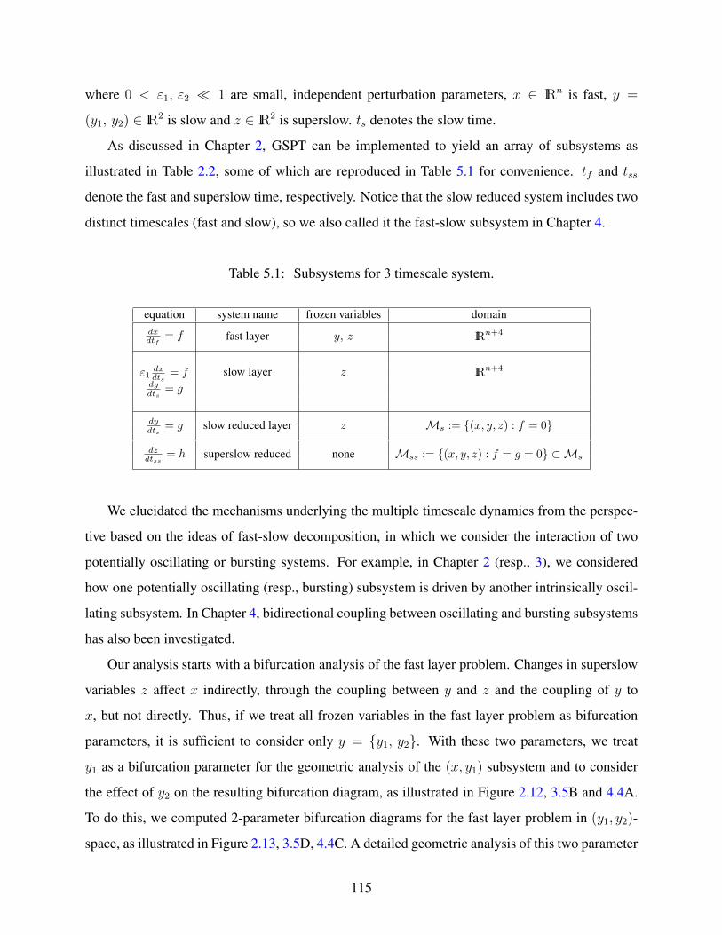
where 0 < ε1, ε2 � 1 are small, independent perturbation parameters, x ∈ IRn is fast, y =
(y1, y2) ∈ IR2 is slow and z ∈ IR2 is superslow. ts denotes the slow time.
As discussed in Chapter 2, GSPT can be implemented to yield an array of subsystems as
illustrated in Table 2.2, some of which are reproduced in Table 5.1 for convenience. tf and tss
denote the fast and superslow time, respectively. Notice that the slow reduced system includes two
distinct timescales (fast and slow), so we also called it the fast-slow subsystem in Chapter 4.
Table 5.1: Subsystems for 3 timescale system.
equation system name frozen variables domaindxdtf
= f fast layer y, z IRn+4
slow layer z IRn+4ε1dxdts
= fdydts
= g
dydts
= g slow reduced layer z Ms := {(x, y, z) : f = 0}
dzdtss
= h superslow reduced none Mss := {(x, y, z) : f = g = 0} ⊂ Ms
We elucidated the mechanisms underlying the multiple timescale dynamics from the perspec-
tive based on the ideas of fast-slow decomposition, in which we consider the interaction of two
potentially oscillating or bursting systems. For example, in Chapter 2 (resp., 3), we considered
how one potentially oscillating (resp., bursting) subsystem is driven by another intrinsically oscil-
lating subsystem. In Chapter 4, bidirectional coupling between oscillating and bursting subsystems
has also been investigated.
Our analysis starts with a bifurcation analysis of the fast layer problem. Changes in superslow
variables z affect x indirectly, through the coupling between y and z and the coupling of y to
x, but not directly. Thus, if we treat all frozen variables in the fast layer problem as bifurcation
parameters, it is sufficient to consider only y = {y1, y2}. With these two parameters, we treat
y1 as a bifurcation parameter for the geometric analysis of the (x, y1) subsystem and to consider
the effect of y2 on the resulting bifurcation diagram, as illustrated in Figure 2.12, 3.5B and 4.4A.
To do this, we computed 2-parameter bifurcation diagrams for the fast layer problem in (y1, y2)-
space, as illustrated in Figure 2.13, 3.5D, 4.4C. A detailed geometric analysis of this two parameter
115

bifurcation structures revealed the mathematical mechanism of solutions to our problem as the two
slow variables traverse (y1, y2)-space: e.g., we used the two parameter bifurcation structures to
understand the mechanisms underlying the regular bursts within both MB and SB solutions in
Chapter 3 and 4, respectively.
Notice that the superslow variable hasn’t come into play, the presence of which determines
on which timescale (slow or superslow) y2 evolves. Understanding this is crucial in explaining
how the transition from the regular burst to the long burst within MB and SB solutions happens.
The mechanism underlying the jump up of y2 in Chapter 3 is easy to understand, since (y2, z)
subsystem (i.e. the (c, l) subsystem) acts as a relaxation oscillator and hence the jumps occur at a
saddle-node bifurcation of this subsystem. However, in the Jasinski model, instead of slaving to
z and evolving on a superslow timescale during the silent phase, y1 exhibits slow drift throughout
the spiking phase of each burst. Hence, we used slow averaged nullcline method, a numerical tech-
nique commonly used in two timescale context when solutions combine fast oscillations and slow
drift [2, 6]. Implementation of the averaging method enabled us to detect the bifurcation corre-
sponding to the transition from the regular burst to the long burst. Combining with the bifurcation
analysis of the fast layer problem, our methods provided us a full explanation of the SB solution
dynamics.
While our study is motivated by the bursting patterns observed in the pre-BotC, it may as well
be applicable to other brain areas exhibiting rhythmic activity. In other mammalian CPGs and
rhythmic neural circuits, the NaP current and CAN current have been identified as playing critical
roles in pattern generation [79, 68, 82, 69, 83, 64, 5, 75]. Given that NaP and CAN currents are
widespread and can be essential for the generation of bursts [56, 14, 73, 47, 30], it seems likely that
the interaction of these currents is a fundamental component of the genesis of bursting solutions in
other areas as well. Therefore, it is likely that our analysis of MB or SB patterns can be extended
and applied to these other rhythmic neuronal systems, both to explain the underlying dynamics and
to assess its timescale requirements.
116
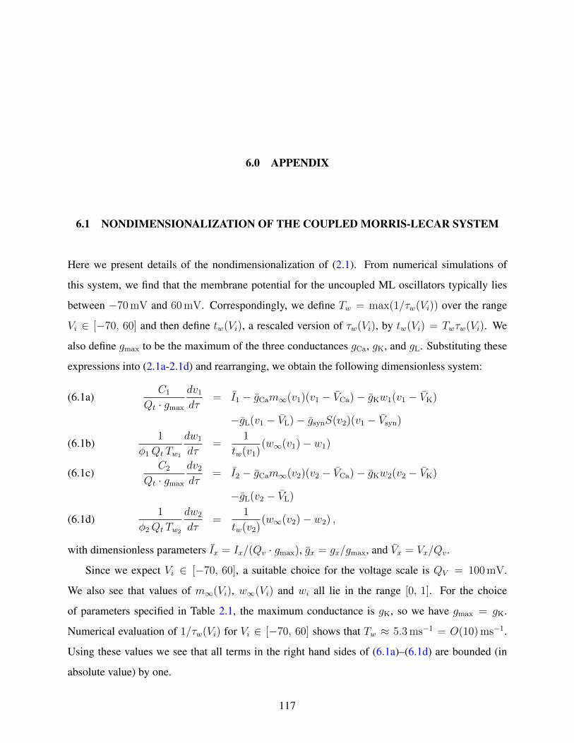
6.0 APPENDIX
6.1 NONDIMENSIONALIZATION OF THE COUPLED MORRIS-LECAR SYSTEM
Here we present details of the nondimensionalization of (2.1). From numerical simulations of
this system, we find that the membrane potential for the uncoupled ML oscillators typically lies
between −70 mV and 60 mV. Correspondingly, we define Tw = max(1/τw(Vi)) over the range
Vi ∈ [−70, 60] and then define tw(Vi), a rescaled version of τw(Vi), by tw(Vi) = Twτw(Vi). We
also define gmax to be the maximum of the three conductances gCa, gK, and gL. Substituting these
expressions into (2.1a-2.1d) and rearranging, we obtain the following dimensionless system:
C1
Qt · gmax
dv1dτ
= I1 − gCam∞(v1)(v1 − VCa)− gKw1(v1 − VK)(6.1a)
−gL(v1 − VL)− gsynS(v2)(v1 − Vsyn)
1
φ1Qt Tw1
dw1
dτ=
1
tw(v1)(w∞(v1)− w1)(6.1b)
C2
Qt · gmax
dv2dτ
= I2 − gCam∞(v2)(v2 − VCa)− gKw2(v2 − VK)(6.1c)
−gL(v2 − VL)
1
φ2Qt Tw2
dw2
dτ=
1
tw(v2)(w∞(v2)− w2) ,(6.1d)
with dimensionless parameters Ix = Ix/(Qv · gmax), gx = gx/gmax, and Vx = Vx/Qv.
Since we expect Vi ∈ [−70, 60], a suitable choice for the voltage scale is QV = 100 mV.
We also see that values of m∞(Vi), w∞(Vi) and wi all lie in the range [0, 1]. For the choice
of parameters specified in Table 2.1, the maximum conductance is gK, so we have gmax = gK.
Numerical evaluation of 1/τw(Vi) for Vi ∈ [−70, 60] shows that Tw ≈ 5.3 ms−1 = O(10) ms−1.
Using these values we see that all terms in the right hand sides of (6.1a)–(6.1d) are bounded (in
absolute value) by one.
117

The coefficients of the derivatives in the left hand sides of (6.1a)–(6.1d) now reveal the relative
rates of evolution of the variables. We find that C1/gmax = O(1) ms−1, 1/(φ1 Tw) ≈ C2/gmax =
O(10) ms−1 and 1/(φ2 Tw) = O(100) ms−1, from which we conclude that v1 evolves on a fast
timescale, w1 and v2 evolve on a slow timescale, and w2 evolves on a superslow timescale. We
choose the slow timescale as our reference time, i.e., pick Qt = 10 ms, and set
ε1 :=C1
Qt · gmax
� 1 , ε2 := φ2Qt Tw � 1 ,(6.2a)
Rw1 := φ1Qt Tw , Rv2 :=Qt · gmax
C2
.(6.2b)
As a result, the dimensionless system (6.1) becomes the system (2.4) given in Section 3.1.1, namely
ε1dv1dτ
= I1 − gCam∞(v1)(v1 − VCa)− gKw1(v1 − VK)(6.3a)
−gL(v1 − VL)− gsynS(v2)(v1 − Vsyn) := f1(v1, v2, w1)
dw1
dτ= Rw1
1
tw(v1)(w∞(v1)− w1) := g1(v1, w1)(6.3b)
dv2dτ
= Rv2(I2 − gCam∞(v2)(v2 − VCa)− gKw2(v2 − VK)(6.3c)
−gL(v2 − VL)) := f2(v2, w2)
dw2
dτ= ε2
1
tw(v2)(w∞(v2)− w2) := ε2g2(v2, w2) ,(6.3d)
with small parameters ε1 and ε2, where Rw1 and Rv2 are dimensionless parameters bounded by
one.
6.2 ADJUSTING TIMESCALES IN THE DENDRITIC SUBSYSTEM
The full model (3.1) is capable of generating an MB solution (Figure 6.1A) with original param-
eter values as given in Table 3.1. From the phase plane for the dendritic subsystem as shown in
Figure 3.1B, we find that ([Ca], l) acts as a relaxation oscillator. However, since the l-nullcline
lies extremely close to the left knee of [Ca]-nullcline (Figure 6.1A), the trajectory projected to
([Ca], l)-space does not jump up to large [Ca] values and transition to the long burst (LB) phase im-
mediately after passing the left knee (yellow circle). Instead, it slowly moves along the l-nullcline
118

for a transient period before jumping up to the right branch (Figure 6.1B and C: from the yellow
circle to the green circle); this effect can be interpreted as the influence of the bifurcation in the
dendritic subsystem initiating the (c, l) oscillation that occurs at a value of [IP3] just below 0.95
[47]. Numerically, we observe that small bursts occur during this period (Figure 6.1A). Therefore,
the existence of such MB solution relies heavily on the nullcline interactions, which can be tuned
by changing [IP3]. To clarify the identification of the timescales involved in the MB behavior and
the assessment of how to group timescales, and to eliminate the sensitivity of MB solutions to the
precise value of [IP3], we increase [IP3] to be 1. As a result, the [Ca]-nullcline moves downward
and hence further from the l-nullcline. Furthermore, we also slow down l by decreasing A from
0.005 to 0.001 so that l ∼ O(1000) ms becomes more separated from [Ca], the delay time of the
jump up of [Ca] at the left knee is significantly decreased, and the dendritic subsystem takes on a
stronger relaxation character.
Remark 5. Although the dendritic subsystem acts as a more standard relaxation oscillator with
new parameter values ([IP3] = 1, A = 0.001), [IP3] is not far enough from the bifurcation value
for the influence of the bifurcation mentioned above to completely vanish. Hence, there is still a
transient delay before [Ca] jumps up at the left knee, but it is much shorter than that with original
parameter values.
6.3 NONDIMENSIONALIZATION OF THE MIXED BURSTING MODEL
From numerical simulations, we find that the membrane potential V typically lies between−60 mV
and 20 mV. Correspondingly, for x ∈ {n, h}, we define Tx = max(1/τx(V)) over the range
V ∈ [−60, 20] and then define tx(V ), a rescaled version of τx(V ), by tx(V ) = Txτx(V ). We also
define gmax to be the maximum of the five conductances gL, gK, gNa, gNaP and gCAN. Furthermore,
we let G([Ca]) = [IP3][Ca]([IP3]+KI)([Ca]+Ka)
and gSERCA([Ca]) = VSERCA[Ca]
K2SERCA+[Ca]2
. Substituting these
expressions into equations (3.1) and rearranging, we obtain the following system:
119

0 2000 4000 6000 8000 10000
−50
−30
−10
10
Time(ms)
V
(A)
0.02 0.04 0.06 0.080.75
0.8
0.85
0.9
0.95
[Ca]
l
(B)
0 2000 4000 6000 8000
0.01
0.03
0.05
Time (ms)
[Ca]
(C)
Figure 6.1: Time series for attracting solutions of the full model (3.1) as well as the bifurcation
structure of the dendritic subsystem with parameter values as in Table 3.1. Green and yellow
symbols mark key points along the solution trajectory (green star: the point with minimum gCANTot;
yellow circle: the point when the trajectory passes the left knee of the [Ca]-nullcline; green circle:
beginning of the long burst (LB).) (A): Time series for V . (B): Enlarged view of part of Figure
3.1B showing the nullclines for [Ca] (red) and l (cyan) for the dendritic subsystem, together with
the MB solution from the upper row. (C): Part of time series of [Ca].
120
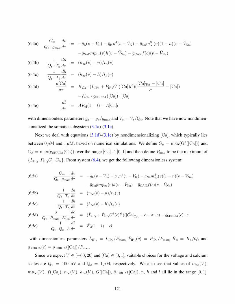
CmQt · gmax
dv
dτ= −gL(v − VL)− gKn4(v − VK)− gNam
3∞(v)(1− n)(v − VNa)(6.4a)
−gNaPmp∞(v)h(v − VNa)− gCANf(c)(v − VNa)
1
Qt · Tndn
dτ= (n∞(v)− n)/tn(v)(6.4b)
1
Qt · Thdh
dτ= (h∞(v)− h)/th(v)(6.4c)
d[Ca]
dτ= KCa · (LIP3 + PIP3G
3([Ca])l3)([Ca]Tot − [Ca]
σ− [Ca])(6.4d)
−KCa · gSERCA([Ca]) · [Ca]
dl
dτ= AKd(1− l)− A[Ca]l(6.4e)
with dimensionless parameters gx = gx/gmax and Vx = Vx/Qv. Note that we have now nondimen-
sionalized the somatic subsystem (3.1a)-(3.1c).
Next we deal with equations (3.1d)-(3.1e) by nondimensionalizing [Ca], which typically lies
between 0µM and 1µM, based on numerical simulations. We define Gc = max(G3([Ca])) and
GS = max(gSERCA(Ca)) over the range [Ca] ∈ [0, 1] and then define Pmax to be the maximum of
{LIP3 , PIP3Gc, GS}. From system (6.4), we get the following dimensionless system:
CmQt · gmax
dv
dτ= −gL(v − VL)− gKn4(v − VK)− gNam
3∞(v)(1− n)(v − VNa)(6.5a)
−gNaPmp∞(v)h(v − VNa)− gCANf(c)(v − VNa)
1
Qt · Tndn
dt= (n∞(v)− n)/tn(v)(6.5b)
1
Qt · Thdh
dt= (h∞(v)− h)/th(v)(6.5c)
σ
Qt · Pmax ·KCa
dc
dτ= (LIP3 + PIP3G
3(c)l3)( ¯[Ca]Tot − c− σ · c)− gSERCA(c) · c(6.5d)
1
Qt ·Qc ·Adl
dτ= Kd(1− l)− cl(6.5e)
with dimensionless parameters LIP3 = LIP3/Pmax, PIP3(c) = PIP3/Pmax, Kd = Kd/Qc and
gSERCA(c) = gSERCA([Ca])/Pmax.
Since we expect V ∈ [−60, 20] and [Ca] ∈ [0, 1], suitable choices for the voltage and calcium
scales are Qv = 100 mV and Qc = 1µM, respectively. We also see that values of m∞(V ),
mp∞(V ), f([Ca]), n∞(V ), h∞(V ), G([Ca]), gSERCA([Ca]), n, h and l all lie in the range [0, 1].
121

For the choice of parameters specified in Table 3.1, the maximum conductance is gNa = 28 nS, so
we have gmax = gNa. Numerical evaluations of 1/τn(V ) and 1/τh(V ) for V ∈ [−60, 20] show that
Tn ≈ 20 ms−1 and Th ≈ 0.04 ms−1. Similarly, we obtain Gc ≈ 0.0421 and GS ≈ 1000 pL ·ms−1,
so we have Pmax ≈ 1305 pL ·ms−1. Using these values we see that all terms in the right hand sides
of equations (6.5a)-(6.5e) are bounded (in absolute value) by one.
The coefficients of the derivatives in the left hand sides of equations (6.5a) - (6.5e) now reveal
the relative rates of evolution of the variables. We find that Cm/gmax = 0.75 ms ∼ O(1) ms,
1/Tn = 0.05 ms ∼ O(0.1) ms, 1/Th = 25 ms ∼ O(10) ms, σPmax·KCa
= 5.67 ms ∼ O(10) ms
and 1Qc·A = 200 ms ∼ O(100) ms. We choose the fast timescale as our reference time, i.e., pick
Qt = 1 ms, and set
Rv :=Cm
Qt · gmax
, Rx :=1
Qt · Tx, x ∈ {n, h},(6.6a)
Rc :=σ
Qt · Pmax ·KCa
, Rl :=1
Qt ·Qc · A.(6.6b)
As a result, the dimensionless system (6.5) becomes the system (3.4) given in Section 3.1,
namely
Rvdv
dτ= −gL(v − VL)− gKn4(v − VK)− gNam
3∞(v)(1− n)(v − VNa)(6.7a)
−gNaPmp∞(v)h(v − VNa)− gCANf(c)(v − VNa) := f1(v, n, h, c)
Rndn
dτ= (n∞(v)− n)/tn(v) := g1(v, n)/tn(v)(6.7b)
Rhdh
dτ= (h∞(v)− h)/th(v) := h1(v, h)/th(v)(6.7c)
Rcdc
dτ= (LIP3 + PIP3G
3(c)l3)( ¯[Ca]Tot − c− σ · c)− gSERCA(c) · c := f2(c, l)(6.7d)
Rldl
dτ= Kd(1− l)− cl := g2(c, l)(6.7e)
where Rv, Rn, Rh, Rc and Rl are dimensionless parameters given in (6.6).
122
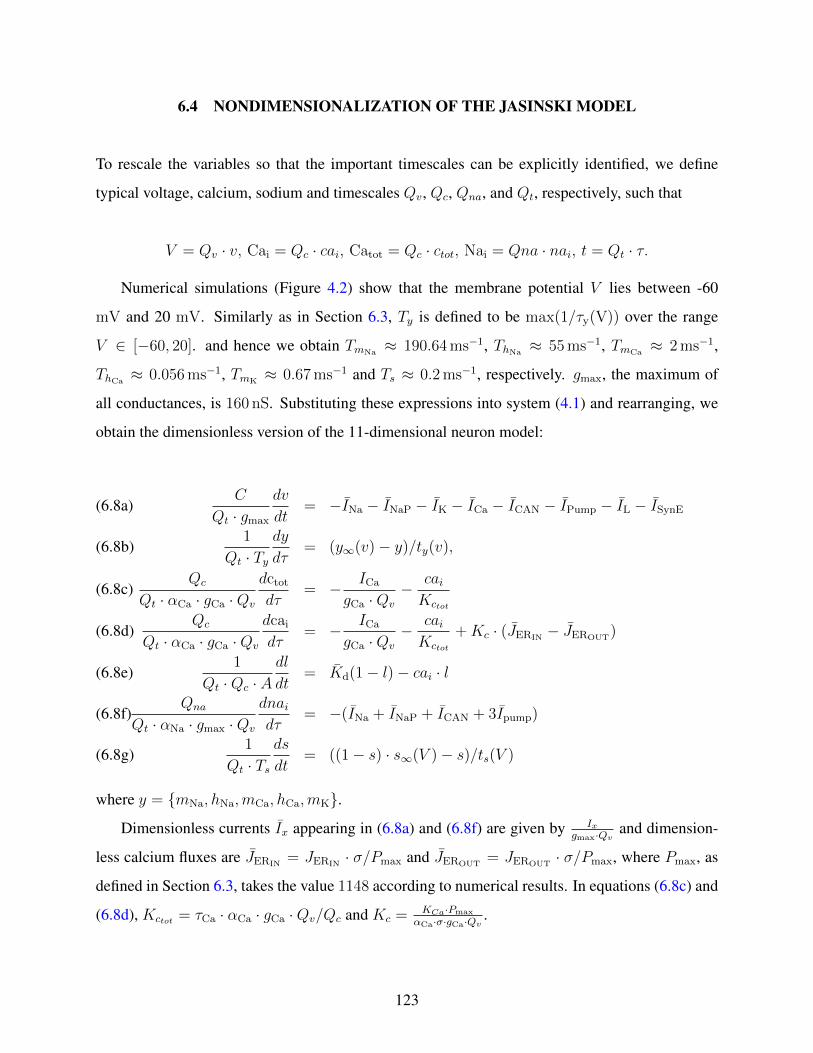
6.4 NONDIMENSIONALIZATION OF THE JASINSKI MODEL
To rescale the variables so that the important timescales can be explicitly identified, we define
typical voltage, calcium, sodium and timescales Qv, Qc, Qna, and Qt, respectively, such that
V = Qv · v, Cai = Qc · cai, Catot = Qc · ctot, Nai = Qna · nai, t = Qt · τ.
Numerical simulations (Figure 4.2) show that the membrane potential V lies between -60
mV and 20 mV. Similarly as in Section 6.3, Ty is defined to be max(1/τy(V)) over the range
V ∈ [−60, 20]. and hence we obtain TmNa≈ 190.64 ms−1, ThNa
≈ 55 ms−1, TmCa≈ 2 ms−1,
ThCa≈ 0.056 ms−1, TmK
≈ 0.67 ms−1 and Ts ≈ 0.2 ms−1, respectively. gmax, the maximum of
all conductances, is 160 nS. Substituting these expressions into system (4.1) and rearranging, we
obtain the dimensionless version of the 11-dimensional neuron model:
C
Qt · gmax
dv
dt= −INa − INaP − IK − ICa − ICAN − IPump − IL − ISynE(6.8a)
1
Qt · Tydy
dτ= (y∞(v)− y)/ty(v),(6.8b)
Qc
Qt · αCa · gCa ·Qv
dctotdτ
= − ICa
gCa ·Qv
− caiKctot
(6.8c)
Qc
Qt · αCa · gCa ·Qv
dcai
dτ= − ICa
gCa ·Qv
− caiKctot
+Kc · (JERIN− JEROUT
)(6.8d)
1
Qt ·Qc · Adl
dt= Kd(1− l)− cai · l(6.8e)
Qna
Qt · αNa · gmax ·Qv
dnaidτ
= −(INa + INaP + ICAN + 3Ipump)(6.8f)
1
Qt · Tsds
dt= ((1− s) · s∞(V )− s)/ts(V )(6.8g)
where y = {mNa, hNa,mCa, hCa,mK}.Dimensionless currents Ix appearing in (6.8a) and (6.8f) are given by Ix
gmax·Qvand dimension-
less calcium fluxes are JERIN= JERIN
· σ/Pmax and JEROUT= JEROUT
· σ/Pmax, where Pmax, as
defined in Section 6.3, takes the value 1148 according to numerical results. In equations (6.8c) and
(6.8d), Kctot = τCa · αCa · gCa ·Qv/Qc and Kc = KCa·Pmax
αCa·σ·gCa·Qv.
123
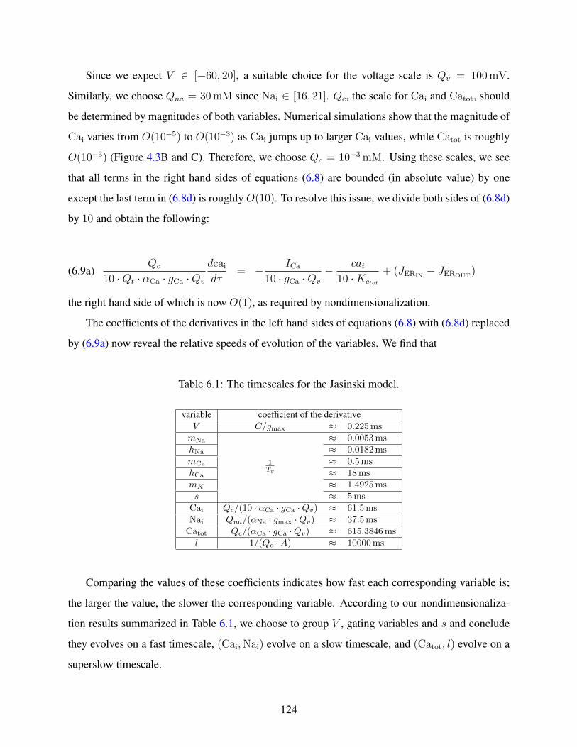
Since we expect V ∈ [−60, 20], a suitable choice for the voltage scale is Qv = 100 mV.
Similarly, we choose Qna = 30 mM since Nai ∈ [16, 21]. Qc, the scale for Cai and Catot, should
be determined by magnitudes of both variables. Numerical simulations show that the magnitude of
Cai varies from O(10−5) to O(10−3) as Cai jumps up to larger Cai values, while Catot is roughly
O(10−3) (Figure 4.3B and C). Therefore, we choose Qc = 10−3 mM. Using these scales, we see
that all terms in the right hand sides of equations (6.8) are bounded (in absolute value) by one
except the last term in (6.8d) is roughly O(10). To resolve this issue, we divide both sides of (6.8d)
by 10 and obtain the following:
Qc
10 ·Qt · αCa · gCa ·Qv
dcai
dτ= − ICa
10 · gCa ·Qv
− cai10 ·Kctot
+ (JERIN− JEROUT
)(6.9a)
the right hand side of which is now O(1), as required by nondimensionalization.
The coefficients of the derivatives in the left hand sides of equations (6.8) with (6.8d) replaced
by (6.9a) now reveal the relative speeds of evolution of the variables. We find that
Table 6.1: The timescales for the Jasinski model.
variable coefficient of the derivativeV C/gmax ≈ 0.225 msmNa
1Ty
≈ 0.0053 mshNa ≈ 0.0182 msmCa ≈ 0.5 mshCa ≈ 18 msmK ≈ 1.4925 mss ≈ 5 ms
Cai Qc/(10 · αCa · gCa ·Qv) ≈ 61.5 msNai Qna/(αNa · gmax ·Qv) ≈ 37.5 ms
Catot Qc/(αCa · gCa ·Qv) ≈ 615.3846 msl 1/(Qc ·A) ≈ 10000 ms
Comparing the values of these coefficients indicates how fast each corresponding variable is;
the larger the value, the slower the corresponding variable. According to our nondimensionaliza-
tion results summarized in Table 6.1, we choose to group V , gating variables and s and conclude
they evolves on a fast timescale, (Cai,Nai) evolve on a slow timescale, and (Catot, l) evolve on a
superslow timescale.
124

BIBLIOGRAPHY
[1] G. F. Alheid, W. K. Milsom, and D. R. McCrimmon. Pontine influences on breathing: anoverview. Respir. Physiol. Neurobiol., 143(2):105–114, 2004.
[2] J. Best, A. Borisyuk, J. Rubin, D. Terman, and M. Wechselberger. The dynamic range ofbursting in a model respiratory pacemaker network. SIAM J. Appl. Dyn. Syst., 4:1107–1139,2005.
[3] C. Beurrier, P. Congar, B. Bioulac, and C. Hammond. Subthalamic nucleus neurons switchfrom single-spike activity to burst-firing mode. J. Neurosci., 19(2):599–609, 1999.
[4] A. Bose, Y. Manor, and F. Nadim. Bistable oscillations arising from synaptic depression.SIAM J. Appl. Math., 62(2):706–727, 2001.
[5] F. Brocard, N. Shevtsova, M. Bouhadfane, S. Tazerart, U. Heinemann, I. Rybak, and L. Vinay.Activity-dependent changes in extracellular Ca 2+ and K+ reveal pacemakers in the spinallocomotor-related network. Neuron, 77(6):1047–1054, 2013.
[6] R.J. Butera, J.W. Clark, and J.H. Byrne. Transient responses of a modeled bursting neuron:analysis with equilibrium and averaged nullclines. Biol. Cybern., 77:307–322, 1997.
[7] R.J. Butera, J. Rinzel, and J.C. Smith. Models of respiratory rhythm generation in the pre-Botzinger complex. i. bursting pacemaker neurons. J. Neurophysiol., 82:382–397, 1999.
[8] R.J. Butera, J. Rinzel, and J.C. Smith. Models of respiratory rhythm generation in the pre-Botzinger complex. ii. populations of coupled pacemaker neurons. J. Neurophysiol., 80:398–415, 1999.
[9] F. Clement and J. Francoise. Mathematical modeling of the gnrh pulse and surge generator.SIAM J. Appl. Dyn. Syst., 6(2):441–456, 2007.
[10] S. Coombes and P.C. Bressloff. Bursting: the genesis of rhythm in the nervous system.
[11] K. Cowley and B. Schmidt. Effects of inhibitory amino acid antagonists on reciprocal in-hibitory interactions during rhythmic motor activity in the in vitro neonatal rat spinal cord. J.Neurophysiol., 74(3):1109–1117, 1995.
125

[12] S. Daun, J. Rubin, and I. Rybak. Control of oscillation periods and phase durations in half-center central pattern generators: a comparative mechanistic analysis. J. Comp. Neurosci.,27:3–36, 2009.
[13] M. Desroches, J. Guckenheimer, B. Krauskopf, C. Kuehn, H.M. Osinga, and M. Wechsel-berger. Mixed-mode oscillations with multiple time scales. SIAM Review, 54:211–288, 2012.
[14] J. Dunmyre, C. Del Negro, and J. Rubin. Interactions of persistent sodium and calcium-activated nonspecific cationic currents yield dynamically distinct bursting regimes in a modelof respiratory neurons. volume 31(2), pages 305–328. 2011.
[15] B. Ermentrout and D. Terman. Mathematical Foundations of Neuroscience. Springer, 2010.
[16] J. Feldman and C. Del Negro. Looking for inspiration: new perspectives on respiratoryrhythm. Nature Reviews Neuroscience, 7(3):232–241, 2006.
[17] J. Feldman and J. Smith. Cellular mechanisms underlying modulation of breathing pattern inmammals. Ann. NY Acad. Sci., 563:114–130, 1989.
[18] N. Fenichel. Persistence and smoothness of invariant manifolds for flows. Indiana Univ.Math. J., 21:193–225, 1971.
[19] N. Fenichel. Geometric singular perturbation theory for ordinary differential equations. vol-ume 31, pages 53–98. 1979.
[20] H. Forster, J. Bonis, K. Krause, J. Wenninger, S. Neumueller, M. Hodges, and L. Pan. Con-tributions of the pre-Botzinger complex and the Kolliker-Fuse nuclei to respiratory rhythmand pattern generation in awake and sleeping goats. Progress in Brain Research, 209:73–89,2014.
[21] A. Franci, G. Drion, and R. Sepulchre. Modeling the modulation of neuronal bursting: Asingularity theory approach. SIAM J. Appl. Dyn. Syst., 13(2):798–829, 2014.
[22] H. Koizumi H and J.C. Smith. Persistent Na+ and K+-dominated leak currents contribute torespiratory rhythm generation in the pre-Botzinger complex in vitro. J. Neurosci., 28:1773–1785, 2008.
[23] J. Ha and A. Kuznetsov. Frequency switching in a two-compartmental model of the dopamin-ergic neuron. J. Comp. Neurosci., 30:241–254, 2011.
[24] E. Harvey, V. Kirk, H.M. Osinga, J. Sneyd, and M. Wechselberger. Understanding anomalousdelays in a model of intracellular calcium dynamics. Chaos, 20:045104, 2010.
[25] E. Harvey, V. Kirk, J. Sneyd, and M. Wechselberger. Multiple timescales, mixed mode oscil-lations and canards in models of intracellular calcium dynamics. J. Nonlin. Sci., 21:639–683,2011.
126

[26] E. Izhikevich. Neural excitability, spiking, and bursting. International Journal of Bifurcationand Chaos, 10:1171–1266, 2000.
[27] E. Izhikevich. Dynamical Systems in Neuroscience: The Geometry of Excitability and Burst-ing. MIT Press, Cambridge, MA, 2006.
[28] E. Izhikevich. Dynamical Systems in Neuroscience. MIT Press, 2007.
[29] J. Jalics, M. Krupa, and H. Rotstein. Mixed-mode oscillations in a three time-scale system ofodes motivated by a neuronal model. Dynamical Systems, 25(4):445–482, 2010.
[30] P. Jasinski, Y. Molkov, N Shevtsova, J. Smith, and I. Rybak. Sodium and calcium mecha-nisms of rhythmic bursting in excitatory neural networks of the pre-Botzinger complex: acomputational modelling study. volume 37, pages 212–230. 2013.
[31] C.K.R.T. Jones. Geometric singular perturbation theory. In Dynamical systems (MontecartiniTerme, 1994), pages 44–118. Springer-Verlag, Berlin, New York, 1995.
[32] T. J. Kaper. An introduction to geometric methods and dynamical systems theory for singularperturbation problems. In Analyzing Multiscale Phenomena Using Singular PerturbationMethods, volume 56 of Proceedings of Symposia in Applied Mathematics, pages 85–131.American Mathematical Society, Providence, RI, 1999.
[33] J. Keener and J. Sneyd. Mathematical Physiology. Springer, 2008.
[34] M. Krupa, N. Popovic, and N. Kopell. Mixed-mode oscillations in three time-scale systems:A prototypical example. SIAM J. Appl. Dyn. Syst., 7(2):361–420, 2008.
[35] M. Krupa, A. Vidal, M. Desroches, and F. Clement. Mixed-mode oscillations in a multipletime scale phantom bursting system. SIAM J. Appl. Dyn. Syst., 11:1458–1498, 2012.
[36] K. Lee, W. Duan, J. Sneyd, and A.E. Herbison. Two slow calcium-activated afterhyperpolar-ization currents control burst firing dynamics in gonadotropin-releasing hormone neurons. J.Neurosci., 30:6214–6224, 2010.
[37] J. J.C. LeGallois. Experiences sur le Principe de la Vie, notamment sur celui des mouvemensdu coeur, et sur le siege de ce principe. A Paris: Chez D’Hautel, 1812.
[38] T. Lumsden. Observations on the respiratory centres in the cat. J. Physiol., 57:153–160,1923.
[39] P. De Maesschalck, E. Kutafina, and N. Popovic. Three time-scales in an extendedBonhoeffer-Van der Pol oscillator. J. Dyn. Diff. Equat., 26:955–987, 2014.
[40] C. Morris and H. Lecar. Voltage oscillations in the barnacle giant muscle fiber. Biophys. J.,35(1):193–213, 1981.
127

[41] P. Nan, Y. Wang, V. Kirk, and J. Rubin. Understanding and distinguishing three-time-scaleoscillations: case study in a coupled morris-lecar system. SIAM J. Appl. Dyn. Syst., 14:1518–1557, 2015.
[42] C. Del Negro, J. Hayes, and J. Rekling. Dendritic calcium activity precedes inspiratory burstsin pre-Botzinger complex neurons. J. Neurosci., 31(3):1017–1022, 2011.
[43] C. Del Negro, C. Morgado-Valle, and J. Feldman. Respiratory rhythm: an emergent networkproperty? Neuron, 34:821–830, 2002.
[44] C.A. Del Negro, J.A. Hayes, R.W. Pace, B.R. Brush, R. Teruyama, and J.L. Feldman. Synap-tically activated burst-generating conductances may underlie a group-pacemaker mechanismfor respiratory rhythm generation in mammals. In: Gossard J-P, Progress in Brain Research.Amsterdam The Netherlands, 2010.
[45] C.A. Del Negro, N. Koshiya, R.J. Butera, and J.C. Smith. Persistent sodium current, mem-brane properties and bursting behavior of pre-Botzinger complex inspiratory neurons in vitro.J. Neurophysiol., 88:2242–2250, 2002.
[46] C.A. Del Negro, C. Morgado-Valle, J.A. Hayes, D.D. Mackay, R.W. Pace, E.A. Crowder,and J.L. Feldman. Sodium and calcium current-mediated pacemaker neurons and respiratoryrhythm generation. J. Neurosci., 25:446–453, 2005.
[47] C. Park and J. Rubin. Cooperation of intrinsic bursting and calcium oscillations underlyingactivity patterns of model pre-Botzinger complex neurons. J. Comp. Neurosci., 34:345–366,2013.
[48] N. Popovic. Mixed-mode dynamics and the canard phenomenon: Towards a classification.In Journal of Physics: Conference Series, volume 138, page 012020. IOP Publishing, 2008.
[49] L.K. Purvis, J.C. Smith, H. Koizumi, , and R.J. Butera. Intrinsic bursters increase the robust-ness of rhythm generation in an excitatory network. J. Neurophysiol, 97:1515–1526, 2007.
[50] J. Ramirez and D. Richter. The neuronal mechanisms of respiratory rhythm generation. Curr.Opin. Neurobiol., 6(6):817–825, 1996.
[51] J. Rekling and J. Feldman. Prebotzinger complex and pacemaker neurons: hypothesized siteand kernel for respiratory rhythm generation. Annual review of physiology, 60(1):385–405,1998.
[52] J. Rinzel. Bursting oscillations in an excitable mebrane model. In Ordinary and partialdifferential equations, volume 1151, pages 304–316. Springer, 1985.
[53] J. Rinzel. A formal classification of bursting mechanisms in excitable systems. In InA.M. Gleason, edtiro, Proceedings of the International Congress of Mathematicians, pages1578–1594. American Mathematical Society, Providence, RI, 1987.
128
[54] J. Rinzel and B. Ermentrout. Analysis of neural excitability and oscillations. pages 251–291,1998.
[55] J. Rubin. Bursting induced by excitatory synaptic coupling in non-identical conditional re-laxation oscillators or square-wave bursters. Phys. Rev. E, 74:021917, 2006.
[56] J. Rubin, J. Hayes, J. Mendenhall, and C. Del Negro. Calcium-activated nonspecific cationcurrent and synaptic depression promote network-dependent burst oscillations. Proc. Natl.Acad. Sci. USA, 106:2939–2944, 2009.
[57] J. Rubin and D. Terman. Geometric singular perturbation analysis of neuronal dynamics.Handbook of dynamical systems, 2:93–146, 2002.
[58] J. Rubin and D. Terman. Synchronized activity and loss of synchrony among heterogeneousconditional oscillators. SIAM J. Appl. Dyn. Syst., 1:146–174, 2002.
[59] J. Rubin and M. Wechselberger. Giant squid-hidden canard: the 3d geometry of the hodgkin-huxley model. Biol. Cybern., 97:5–32, 2007.
[60] I. A. Rybak, R. O’connor, A. Ross, N. A. Shevtsova, S. C. Nuding, L. S. Segers, ..., andI. C. Solomon. Reconfiguration of the pontomedullary respiratory network: A computationalmodeling study with coordinated in vivo experiments. J. Neurophysiol., 100(4):1770–1799,2008.
[61] I.A. Rybak, K. Ptak, N.A. Shevtsova, and D.R. McCrimmon. Sodium currents in neuronsfrom the rostroventrolateral medulla of the rat. J. Neurophysiol., 90:1635–1642, 2003.
[62] L. S. Segers, S. C. Nuding, T. E. Dick, R. Shannon, D. M. Baekey, I. C. Solomon, K.F. Morris,and B. G. Lindsey. Functional connectivity in the pontomedullary respiratory network. J.Neurophysiol., 100(4):1749–1769, 2008.
[63] X. Shao and J. Feldman. Respiratory rhythm generation and synaptic inhibition of expira-tory neurons in pre-botzinger complex: differential roles of glycinergic and gabaergic neuraltransmission. J. Neurophysiol., 77:1853–1860, 1997.
[64] M. Sheroziya, O. von Bohlen, K. Unsicker, and A.V. Egorov. Spontaneous bursting activityin the developing entorhinal cortex. J. Neurosci., 29:12131–12144, 2009.
[65] J. Smith, H. Ellenberger, K. Ballanyi, D. Richter, and J. Feldman. Pre-botzinger complex: abrainstem region that may generate respiratory rhythm in mammals. Science, 254:726–729,1991.
[66] J.C. Smith, A.P. Abdala, H. Koizumi, I.A. Rybak, and J.F. Paton. Spatial and functionalarchitecture of the mammalian brain stem respiratory network: a hierarchy of three oscillatorymechanisms. J. Neurophysiol., 98:3370–3387, 2007.
[67] D. Somers and N. Kopell. Rapid synchronization through fast threshold modulation. Biol.Cybern., 68:393–407, 1993.
129

[68] S. Tazerart, J. Viemari, P. Darbon, L. Vinay, and F. Brocard. Contribution of persistent sodiumcurrent to locomotor pattern generation in neonatal rats. J. Neurophysiol., 98(2):613, 2007.
[69] S. Tazerart, L. Vinay, and F. Brocard. The persistent sodium current generates pacemakeractivities in the central pattern generator for locomotion and regulates the locomotor rhythm.J. Neurosci., 28:8577–8589, 2008.
[70] D. Terman, N. Kopell, and A. Bose. Dynamics of two mutually coupled inhibitory neurons.Physica D, 117:241–275, 1998.
[71] D. Terman and D. Wang. Global competition and local cooperations in a network of neuraloscillators. Physica D, 81:148–176, 1995.
[72] M. Thoby-Brisson and J.M. Ramirez. Identification of two types of inspiratory pacemakerneurons in the isolated respiratory neural network of mice. J. Neurophysiol., 86:104–112,2001.
[73] N. Toporikova and R.J. Butera. Two types of independent bursting mechanisms in inspiratoryneurons: an integrative model. J. Comp. Neurosci., 30(3):515–528, 2011.
[74] K. Tsumoto, H. Kitajima, T. Yoshinaga, K. Aihara, and H. Kawakami. Bifucations in Morris-Lecar model. Neurocomputing, 69:293–316, 2006.
[75] K. Tsuruyama, C.-F. Hsiao, and S. Chandler. Participation of a persistent sodium currentand calcium-activated nonspecific cationic current to burst generation in trigeminal principalsensory neurons. J. Neurophysiol., 110(8):1903–1914, 2013.
[76] A. Vidal and F. Clement. A dynamical model for the control of the gonadotrophin-releasinghormone neurosecretory system. J. Neuroendocrinology, 22(12):1251–1266, 2010.
[77] T. Vo, R. Bertram, and M. Wechselberger. Multiple geometric viewpoints of mixed modedynamics associated with pseudo-plateau bursting. SIAM J. Appl. Dyn. Syst., 12(2):789–830,2013.
[78] T. Vo, J. Tabak, R. Bertram, and M. Wechselberger. A geometric understanding of howfast activating potassium channels promote bursting in pituitary cells. J. Comp. Neurosci.,36(2):259–278, 2014.
[79] D. Wang, S. Grillner, and P. Wallen. Effects of flufenamic acid on fictive locomotion, plateaupotentials, calcium channels and NMDA receptors in the lamprey spinal cord. Neurophar-mocology, 51:1038–1046, 2006.
[80] Y. Wang and J. Rubin. Multiple time scale mixed bursting dynamics in a respiratory neuronmodel. J. Comp. Neurosci., pages 1–24, 2016.
[81] M. Wechselberger. A propos de canards (apropos canards). Trans. Am. Math. Soc, 364:3289–3309, 2012.
130

[82] G. Zhong, M. Masino, and R. Harris-Warrick. Persistent sodium currents participate in fictivelocomotion generation in neonatal mouse spinal cord. J. Neurosci., 27(17):4507–4518, 2007.
[83] L. Ziskind-Conhaim, L. Wu, and E.P. Wiesner. Persistent sodium current contributes to in-duced voltage oscillations in locomotor-related hb9 interneurons in the mouse spinal cord. J.Neurophysiol., 100(4):2254–2264, 2008.
131