analysis of atmospheric dischargegpc-whitepapers.com/uploads/media/atmospheric discharge.pdf ·...

Analysis of Atmospheric Discharge Qualitative and Quantitative Safety Screening

John Burgess, P.E. Dustin Smith, P.E.

Phone: 713.802.2647 [email protected] www.smithburgess.com

mailto:[email protected]

http://www.smithburgess.com/

Disclaimer: This paper is offered for general informational purposes only. Readers should consult with a qualified profession regarding their specific projects or work. The authors disclaim any and all liability arising from or concerning the analysis contained in this paper.

Abstract The design of relief/venting systems is imperative in facilities because existing installations or other design requirements frequently result in the potential for atmospheric releases. To ensure atmospheric discharges are to a safe location as required by good engineering practice [e.g. ASME Section VIII UG-135 (f)], facilities should consider the qualitative requirements, decision making processes, and quantitative methods summarized in this paper.

This paper can be used as the basis for analyzing new and existing facilities. The first section of this paper details qualitative considerations to ensure that the discharge location is safe. The following sections provide quantitative and semi-quantitative means to verify that the concentration of flammables and toxic material is within specified limits. The final portion of this paper contains information typically required to perform dispersion modeling. The purpose of this paper is to simplify existing methods, such that typical plant engineers with everyday tools can screen most atmospheric releases.

Detailed dispersion modeling was performed to validate the results of the simplified equations presented in this paper. Under the most common conditions that hydrocarbon streams are processed, the methods in this paper are conservative and can be used to screen atmospheric relief device installations.

Introduction The design of atmospheric relief/venting systems is imperative in facilities because existing installations or other design requirements frequently result in the potential for atmospheric releases. Recent accidents and regulatory pressure have many companies asking:

How many relief valves do we have going to atmosphere? Are these relief valves safe? Can we prove that they are safe?

To ensure atmospheric discharges are to a safe location as required by good engineering practice, engineers and designers should follow a systematic decision making process. This paper presents qualitative requirements and quantitative screening methods.

Each situation is unique and may have characteristics that require special consideration. The author once overheard an engineer complaining that his company had recently lost a court case. His site had a release that was well below any level that could cause harm to the public, but you could smell the chemicals. This release floated into an elementary school; the students smelled the chemicals but were otherwise unaffected. He seemed incredulous that his company lost this court case, but really, while unfair, why is this not the most obvious outcome? The installation at his site would pass all the criteria presented in this paper, but good engineering judgment should have proposed additional mitigation, or at the least, elevated this concern for the appropriate risk based review.

The vast majority of atmospheric releases from petrochemical and refining facilities are from relief devices. The focus of this paper is safe atmospheric relief device design. Methods and designs necessary to comply with environmental regulations are not discussed and must be independently verified.


Section I – Qualitative Screening Criteria The requirements for the safe disposal of effluent streams dictate a higher level of safety for designed releases versus an un-designed loss of containment. Consider the following two cases:

1. An amine regenerator overpressures and the relief device works as designed. This system is in a gas plant and the relief device final disposition is from an atmospheric collection system. The resulting vapor cloud results in H2S area monitors activating and the evacuation of all non-essential personnel from the site. The unit also shuts down.

2. A fork truck driver is delivering some equipment near the amine regenerator and backs into piping, resulting in a leak from a control valve station. This leak creates a vapor cloud that activates H2S monitors. Consequently, all non-essential personnel from the site are evacuated and the unit shuts down.

Which case is worse? Arguably both could be prevented with better engineering design, but in the first scenario the overpressure system functioned as designed and yet the facility was evacuated. This paper will help engineers design safe installations such that the first scenario would not occur. This paper is focused on designed releases (e.g. relief device tail piping) as compared to facility siting concerns associated with loss of containment scenarios (e.g. vessel ruptures).

Venting Sources Types

Atmospheric venting is designed into many petrochemical and refining facilities. Generally, designed or planned atmospheric releases come from several sources:

Control Systems – Backpressure regulators, compressor stability control schemes, and Emergency Shutdown Devices can discharge to the atmosphere. To determine the safety of these systems, the engineer needs to consider the discharge fluid, the specifics of the control system, as well as the final location of the vent.

Pressure Relief Devices – Pressure relief valves, rupture disks, and conservation vents can all have installations that discharge the effluent directly to the atmosphere.

Atmospheric Collections Systems – These systems can range from the collection of one or two relief devices into a single vent stack to systems as complex as flare systems terminating with a vent instead of a flare tip. Special considerations are required for the analysis of the vent, as there is no designed means to burn the combustible material. These systems may or may not include blowdown drums and/or tanks. Blowdown drums and tanks remove the liquids from the vapor and send the vapor to atmosphere.

Flare Systems – Flare systems are designed to capture the effluent from the facility, remove entrained liquids, and to burn the remaining vapor. Even though most engineers do not consider flare systems to be atmospheric discharges, the combustion products are ultimately released to the atmosphere. Also, the effluent can be discharged directly to the atmosphere in the event of a loss of the pilots or a loss of combustion.

Each of these systems can be designed safely with proper consideration for the toxicity and flammability of the fluid and the design of the vent/flare. While no regulatory rules apply, the following qualitative screening considerations should be reviewed.


Non-flammable/Combustible and Non-toxic Fluids

These are the safest systems to discharge to atmosphere since they rarely result in large-scale harm. When analyzing the location of the discharge, consider the following:

Effects on Personnel – A vent cannot be “safe” if it may come into contact with employees. Direct contact of a hot fluid such as steam or water could cause burns. Vapor liquid mixtures or those which may condense (e.g. saturated steam) may result in the liquids “raining” down, even if the discharge is directed upwards.

o Impingement – The velocity of the fluid also has the potential to injure individuals who may be in the discharge path. When analyzing the impingement of an effluent on personnel, the engineer should analyze the immediate disposition of the fluid as well as the subsequent movement of the fluid. The analysis should include nearby work areas, walkways, ladders, and other areas designed for occupancy. If it is determined that no adverse health effects are expected as a result of the discharge, continue to the next item.

o Oxygen Deficient Atmosphere – A large release of nitrogen or steam into a building or confined area could dilute the oxygen in the atmosphere and thus make the area uninhabitable. Common industrial gasses, like nitrogen, helium, and argon, are classified as simple asphyxiants.

o Emergency Operations – The ability of operators to safely perform emergency procedures during a release should be considered. If a nearby isolation valve requires manual operation during a release, the designer needs to consider the effect of the release on the operator.

Public Relations – Another consideration is the effect the release may have on the public. The designer needs to consider if a system will routinely release. Releases should be reviewed for the potential to form “clouds,” loud noises, or odors. Any of these factors may interfere with operations or cause concern with the public.

A discharge of “safe” fluids still requires analysis to ensure that the installation is acceptable.

Flammable and/or Combustible Fluids

These releases require more engineering review than non-flammable/non-toxic releases. In addition to the analyses above, the following considerations need to be reviewed:

Vapor Releases – Most industrial processes have hydrocarbons above the upper flammable concentration to prevent explosions and/or fires in the piping. A release of flammable material travels from the process concentration, through the upper flammable limit (UFL), through a flammable concentration limit, and finally passes through the lower flammable limit (LFL), and ceases to be a fire or explosion risk. Figure 1 is an illustration of a release from a nozzle that has caught fire. The area prior to the flames is too rich to burn above the upper flammable limit. All releases of potentially flammable material must be reviewed to ensure that the fluid has safely passed

Figure 1: Drawing of an ignited release. © sxc. Image by G Fordham.


through the LFL before the “cloud” reaches a point of interest (e.g. an ignition source: grade, platform, equipment, etc.). API STD 521 specifies a 2× safety factor by stating that points of interest should not exceed 50% of the LFL for existing facility and 10% of the LFL for new facilities.

Liquids/solid Releases – Scenarios that could release flammable liquids or solids to atmosphere are generally not acceptable and require mitigation. The release case either needs to be mitigated through:

1. Dedicated safety instrumentation (e.g. compliant with ISA S-84) to the point that the release is not credible

2. The system design must ensure that the liquids/solids are contained and not vented (e.g. blowdown drum or tank).

At the time of writing this paper, the commercially available dispersion modeling software does not accurately predict dispersion of liquids/solids. Unless engineers/designers can validate the model findings, the validity of the predicted flammable concentrations at points of interest may not be useful.

Toxic Fluids

In addition to the all of the previously identified considerations, toxic fluid release should consider:

Vapor Releases – The concentration of the toxic component in the release decreases from the effluent concentration to zero at some distance downwind. Determining an acceptable lower concentration can be difficult, but there are a variety of sources that offer guidance (see Table 7).

Liquid Releases – Releasing toxic, volatile liquids directly to the atmosphere should be avoided. The discharge of liquids that are non-volatile (e.g. caustic) may be acceptable; however, they are not further discussed in this paper.

Section II – Quantitative Screening Criteria There are many quantitative and semi-quantitative methods to analyze the safety of atmospheric releases. The methods presented in this paper are useful for screening and have been simplified for easier implementation. All of the methods presented are general and may not account for the specifics of each installation. Borderline acceptability or special circumstance may require detailed modeling to be determined by the engineer/designer.

Semi-Quantitative Analysis of Atmospheric Discharge

The discharge of potentially flammable or toxic material to atmosphere is not preferred. However, the risks associated with atmospheric releases can be minimized by designing the system carefully. An extensive review of incident reports from various databases, including the Major Accident Reporting System [MARS], Major Hazard Incident Data Service [MHIDAS], and the National Fire Information Reporting System [NFIRS], concludes that incidents associated with atmospheric releases from relief devices are very rare. With proper design, vertically pointed relief device discharges have historically been a safe means of disposing vapors. The following sections of this paper illustrate semi-quantitative and quantitative methods to determine if an atmospheric discharge is safe.


Relief Devices Types It is important to note that this discussion applies only to pop action relief devices and not modulating relief devices. Pop action relief devices are designed to "pop" open. They also close when the velocity fluid is about 25% of the valve’s capacity. In contrast, a modulating relief device will open enough to pass the required relief rate, and thus may flow significantly less fluid than a pop action relief device.

Due to minimal flow conditions of pop action relief devices, there are predictable momentum and velocity mixing effects. The correlations presented are based on these mixing effects and do not predict the acceptability of atmospheric release from modulating relief devices. Therefore, all discussions are limited to pop action type relief devices.

Flammable and Toxic Concerns The primary concern when analyzing atmospheric releases is the potential to form a flammable or toxic cloud near ignition sources or workers. API STD 521 5th ed. Guide for pressure relieving and depressuring systems §6.3 provides a series of guidelines to determine if a relief device to atmosphere is acceptable based on the “jet” momentum and velocity mixing effects of the discharge. The greater the exit velocity, the more turbulent the material mixes with air. This results in the concentration of the released material quickly reducing below the LFL. Additionally, higher velocities from vertically directed vents are more vertical than horizontal. To semi-quantitatively determine if a release is acceptable, the following criteria must be met (per API STD 521 §6.3):

Exit velocity greater than 100 ft/s Ratio of the exit velocity to wind velocity greater than 10 Vapor MW less than 80 No equipment or work areas at or above the release point horizontally for 50 ft Relief/jet temperatures that are near or above atmospheric temperature Previously listed qualitative considerations reviewed

If the exit velocity is 100 ft/s, the wind speed required to meet the second criteria is 10 ft/s or ~6.8 mph. Further in the paper, Table 6 shows the wind speed probabilities for various locations. Table 1 shows an analysis of these criteria for a release of Y grade pipeline fluid with the exit piping the same diameter as the outlet of the relief device.

Table 1: Calculated Exit Velocities with API RP 521 Momentum Criteria for a 6Q8 a Relief Valve

Scenario

Valve Capacity

(lb/hr)

Exit Velocity

(ft/s)

Jet / Wind Ratio

Jet > 100 ft/s Acceptable

Rate Capacity 83,554 460 94 Yes Yes

Blocked Outlet Required Rate 41,862 230 47 Yes Yes

75% of the Rated Capacity 62,665 345 70 Yes Yes



10% of the Rated Capacity* 8,355 46 9 No No

*Note that the analysis at 10% of the rated capacity was included for illustrative purposes only.

A more detailed analysis is required if the installation does not meet all of the listed criteria. Consider either dispersion modeling or the analysis in the following section.


The listed criteria above can be applied to toxic chemicals as well. The diffusion/dilution effects apply to all constituents of the effluent. The basis of the criteria is that a hydrocarbon will dilute from 100% to approximately 3% the estimated lower flammable limit; therefore, the relief fluid will dilute to approximately 30 times the original concentration. The major difference between flammability and toxicity screening requirements is that the limiting concentrations are smaller. Consider H2S, which is toxic and has maximum 10 minute peak exposure limit of 50 ppm for personnel (29 CFR 1910.1000 TABLE Z-2).

Eq. (1) estimates the maximum concentration that a toxic compound can have in the effluent stream to be diluted to the concentration of interest. This is the point where the velocity of the fluid slows down and the jet mixing effects are lost. If there is the potential for personnel in the vicinity of this area, detailed screening may be required. Eq. (1) was obtained from the verbiage in API STD 521 §6.3 based on the statement that the released fluid is diluted 30 to 50 times prior to the loss of the jet mixing effects.

30

Effluent

Limit

CC Eq. (1)

Where:

CLimit = the highest concentration that meets the risk acceptance for the toxic material (ppm, see Table 7)

CEffluent = the concentration of the toxic material in the effluent stream (ppm)

For systems that meet the qualitative and quantitative criteria listed and the concentration limits satisfy Eq. (1), the maximum toxic concentration workers may be exposed to should be below the concentration that meets the risk acceptance criteria. For example, if the fluid in Table 1 had an H2S concentration of 1,500 ppm (or less), then the peak exposure will be below the in-limit of 50 ppm for locations personnel are present.

This type of analysis has limited applicability for streams that contain high concentrations of toxics or for public exposure limits. The ERPG-3 level, a public exposure limit from the American Industrial Hygiene Association, for H2S is 0.1 ppm. This simplified analysis is extremely conservative and should be limited to evaluations of hazards in the immediate vicinity of the relief device and not applied to public exposure. For systems that fail this criteria, consider detailed dispersion modeling or use the more detailed dispersion estimates presented later in this paper.


Quantitative Analysis of Atmospheric Discharge

This section details the analysis of releases from atmospheric vents and is based on API STD 521 Figures 4 and 6. For low velocity releases, when the ratio of the release velocity to the wind speed

is below 10, the assumptions of the dispersion models presented may not be valid. Under these conditions, concentrations may remain in the flammable limits longer, and therefore, detailed dispersion modeling is recommended. Figure 2 depicts an atmospheric release as the concentration of effluent starts above the UFL, is within the flammability limits, and then drops below the LFL. This section of the paper is to simplify the analysis presented in API STD 521 Figures 4 and 6. In addition, since the vertical requirements calculated in API are to the cloud centerline, dispersion modeling was performed to check the validity of these criteria. The horizontal distance to below the LFL is based on API STD 521 Figure 5. The guidance in the API Standard on vertical distance (the dashed line) to the bottom of the flammable cloud is not provided; instead the guidance provided gives the distance to the center line of the cloud.

Based on the dispersion modeling to test API STD 521 Figure 5 (described in Table 2), as much as 1/6 to 1/3 of the cloud height may be between the cloud centerline and the lowest point where the LFL is present. As such, detailed dispersion modeling should be completed if there is equipment above the discharge location within the horizontal distance predicted by either Eq. (5) or Eq. (6), which are adapted from the API criteria.

Figure 3: A cubic fit of API STD Figure 5, Downwind Distance to LFL for Hydrocarbons

y = 19,301x3 - 5,660x2 + 334x + 37.9 R² = 0.9976

0.0

5.0

10.0

15.0

20.0

25.0

30.0

35.0

40.0

45.0

50.0

0 0.02 0.04 0.06 0.08 0.1 0.12 0.14

API STD 521 Figure 5 Cubic Fit

ju

u

j

jd

x

Horizontally to 0.67djvMW

Do not locate

equipment or work areas

above the lower dashed line

Below LFL

Given:

u8 / uj ˜ 0.036

Pj / P8 ˜ 1

T8 / Tj ranges from ½ to 1, assumed to be 1

See also the derivation of Equation 5

Information is based on Figure 7 from API STD 521

Vertically

120 pipe ?

to centerlineAbove UFL

Between

UFL and LFL

Figure 2: Criterion from API RP 521


The maximum downwind horizontal distance from jet exit to lean-flammability concentration limit for petroleum gases (Figure 5 from API STD 521) can be expressed as follows:

9.37334660,5301,19

12

23

jjjjj u

u

u

u

u

u

d

x

Eq. (2)

Where:

x = the horizontal distance downwind to the LFL for a hydrocarbon release (ft)

dj = the inside diameter of the jet release exit (in)

ρj = the density of the fluid just inside the tip exit (lb/ft³)

ρ∞ = the density of the ambient air (lb/ft³)

uj = the fluid jet exit velocity (ft/s)

u∞ = the wind speed (ft/s, see also Table 6)

For a perfect gas,

P

P

T

TMW

PMW

RT

RT

PMWthus

RT

PMW j

j

j

j

jjj

8.28,;

Eq. (3)

Where:

MWj = the molecular weight of the jet release fluid

MW∞ = the molecular weight of the atmosphere, 28.8

Pj = the pressure of the fluid just inside the tip exit, which is typically atmospheric pressure in the case of a pipe exit (psia)

P∞ = the pressure of the ambient air / atmosphere (psia)

Tj = the fluid jet exit temperature (°R)

T∞ = the temperature of the ambient air / atmosphere (°R)

The following is the result of substituting Eq. (3) into Eq. (2) and solving for the distance downwind to the lower flammability limit:

P

P

T

TMWd

x

d

x

j

j

jjjj

8.281212

Eq. (4)


9.37334660,5301,198.2812

23

jjj

j

j

jj

u

u

u

u

u

u

P

P

T

TMWdx Eq. (5)

With the following conservative assumptions, Eq. (5) can be further simplified:

ju

u ≈ 0.036, the maximum downwind extents of the LFL

P

Pj ≈ 1, the pressure at the maximum vent velocity is near atmospheric

jT

T ranges from ½ to 1, and is assumed to be 1. For an atmospheric temperature of 70 °F, the

release temperature would be limited between 70 °F and 600 °F or less for this assumption.

jj

jjMWd

MWdx 67.05.43

8.2812

Eq. (6)

Simplified Model Check

Two hundred and sixteen unique dispersion models were completed in PHAST each with 3 different weather conditions for the different releases shown in Table 2. Each of the cases in Table 2 was run for 1½G3, 4M6, and 6Q8 relief devices. The discharge point is the same pipe diameter as the relief device outlet. The weather used were 3.5 (ft/s), 5 (ft/s), and 10 (ft/s) all with an atmospheric stability class of D. The cases were run at the full capacity of the relief device (as determined by PHAST) and 25% of the rated relief device capacity.

Table 2: Fluid Conditions for the Dispersion Models Run to Compare Against Eq. (6)

Fluid

Pressure (psig)

Cold (F)

Hot (°F)

Ethane 50 0 100 Ethane 250 50 100 n-Pentane 50 200 400 n-Pentane 250 325 400 n-Octane 50 375 600 n-Octane 250 525 600

For each of the cases reviewed, Eq. (6) predicted the extent of the flammable zone to be 30% to 200% farther than the horizontal distance predicted by the PHAST modeling. Also, for the smaller diameter vents with lower MW fluids, Eq. (6) tended to over predict the horizontal distance by 30% or more. For the larger vents with higher MW fluids, Eq. (6) tended to over predict the horizontal distance as much as 200%.


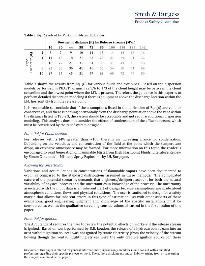
Table 3: Eq. (6) Solved for Various Fluids and Exit Pipes

Downwind distance (ft) for Release Streams (MWj)

16 30 44 58 72 86 100 114 128 142

Pip

e

Dia

me

ter

(dj)

2 5 7 9 10 11 13 14 14 15 16

4 11 15 18 21 23 25 27 29 31 32

6 16 22 27 31 34 38 41 43 46 48

8 22 30 36 41 46 50 54 58 61 64

10 27 37 45 51 57 63 68 72 76 80

Table 3 shows the results from Eq. (6) for various fluids and exit pipes. Based on the dispersion models performed in PHAST, as much as 1/6 to 1/3 of the cloud height may be between the cloud centerline and the lowest point where the LFL is present. Therefore, the guidance in this paper is to perform detailed dispersion modeling if there is equipment above the discharge location within the LFL horizontally from the release point.

It is reasonable to conclude that if the assumptions listed in the derivation of Eq. (6) are valid or conservative, and there is nothing horizontally from the discharge point at or above the vent within the distance listed in Table 3, the system should be acceptable and not require additional dispersion modeling. This analysis does not consider the effects of condensation of the effluent stream, which must be considered by the relief system designer.

Potential for Condensation

For releases with a MW greater than ~100, there is an increasing chance for condensation. Depending on the velocities and concentration of the fluid at the point which the temperature drops, an explosive atmosphere may be formed. For more information on this topic, the reader is encouraged to read Generation of Flammable Mists from High Flashpoint Fluids: Literature Review by Simon Gant and/or Mist and Spray Explosions by J.H. Burgoyne.

Allowing for Uncertainty

Variations and accumulations in concentrations of flammable vapors have been documented to occur as compared to the standard distributions assumed in these methods. The complicated nature of the potential scenarios demands that engineers/designers account for both the natural variability of physical process and the uncertainties in knowledge of the process1. The uncertainty associated with the input data is an inherent part of design because assumptions are made about atmospheric conditions, flows, and physical conditions. The user is cautioned to design for a safety margin that allows for inherent errors in this type of estimation. As with other aspects of these evaluations, good engineering judgment and knowledge of the specific installations must be considered, as well as the qualitative screening considerations discussed in the first section of this paper.

Potential for Ignition

The API Standard requires the user to review the potential effects on workers if the release stream is ignited. Based on work performed by D.E. Loudon, the release of a hydrocarbon stream into an area without ignition sources was not ignited by static electricity (from the velocity of the stream flowing though the vent)2. Lightning strikes were the only credible ignition source for these


Immediately Dangerous to Health or Life (IDLH) Per the OSHA Website, a concentration from which a worker could escape without injury or without irreversible health effects.3

streams. Since the likelihood of a release into an area without ignition sources igniting is extremely rare, higher thermal radiation exposures than are allowed for flare systems may be justified. API STD 521 Table 9 lists recommended limits for personnel exposure to thermal radiation. 2,000 btu/hr/ft² is oftentimes the acceptable maximum thermal radiation from a flare stack in areas where workers may be present. Many organizations have a higher threshold for vent stacks. The authors have seen values of 3,000 btu/hr/ft² or more used.

For a release height of 50 feet, all of the releases modeled in PHAST (Table 2) had maximum ground level thermal radiation below 3,000 btu/hr/ft² and would be considered acceptable by the authors if the facility’s main evacuation route was not affected.

Section III–Quantitative Analysis of Far Field Effects (Toxics) When evaluating the safety of atmospheric releases of a potentially toxic stream, the far field effects must be considered. An example of such a compound is phosgene, which has an IDLH value of 2 ppm versus the LFL of hydrocarbons of 30,000 PPM (or 3%). The distance that must be considered for toxic materials can be significantly farther than that of just flammable fluids. Consequently, the effects of atmospheric stability become much more important.

The analysis presented here assumes a Gaussian distribution for the concentration near the centerline of the release. The centerline is the origin and Eq. (7) described the concentration distribution through the cloud (Weber5).

2

2

2

2

1)(

x

exf Eq. (7)

Where:

= the standard deviation

= the locus of the mean

x = the downwind distance (ft)

The key parameter in the distribution is the standard deviation. Figure 4 shows the effect of the standard deviation on the predicted results. With a lower standard deviation (, the cloud travels farther downwind, but is narrower than compared to a cloud with a higher standard deviation (.


Figure 4: Gaussian Distribution, Relative cloud widths for Standard Deviation of 12 Right and 25 Left

The dispersion of the cloud occurs in both the horizontal and vertical planes. To estimate the concentration of a released material at some point downwind, the standard deviation for both the y and z directions are required.

The most widely accepted method for characterizing meteorological conditions is the atmospheric stability classes developed by Pasquill and Gifford and correlated by Turner.4 Figure 5 depicts the vertical and horizontal parameters that describe the standard deviation for releases in various atmospheric stability classes (A, D, and F are the atmospheric stability classes that are further described in Table 6).

Figure 5: Correlation of Vertical Dispersion Coefficients, z and y, from Turner 1969

0

0.005

0.01

0.015

0.02

0.025

0.03

0.035

-50 0 50

f(x)

0

0.002

0.004

0.006

0.008

0.01

0.012

0.014

0.016

0.018

-50 -30 -10 10 30 50

f(x)

0

0.5

1

1.5

2

2.5

3

2 2.5 3 3.5 4 4.5 53

30

300

3000

0.1 1 10 100

zlog

Xlog

y

x

A

D

F

F

D

A


By applying the Gaussian distribution assumption to dispersion, the following generalized equation describes the concentration at some point downwind of the release (Weber5):

2

2

2

2

2

2

222

2zzy

HzHzy

zy

eeeu

QC

Eq. (8)

Where:

Q source rate (lbm/s) u wind speed (ft/s) y & z standard deviations of the concentration distributions in the y and z directions

(Figure 5) H H is the effective height above grade, the height of release point plus the height

of the plume rise (ft) x the downwind distance (ft) y cross wind distance (ft) z vertical rise above grade (ft) C concentration (lbm/ft³)

To determine the concentration at grade on the centerline downwind [z=0, y=0, Eq. (8)] simplifies as follows:

2

2

2

2z

H

zy

eu

QC

Eq. (9)

Downwind Distance to Maximum Concentration at Grade

Eq. (10) is the derivative of Eq. (8) for the concentration with respect to downwind distance. Because we are only looking at the downwind concentration (as opposed to the concentration variation cross), only z is a function of x.

dx

dHe

u

Q

dx

dC z

z

y

y

y

122 2

22 2

2

Eq. (10)

The maximum concentration at grade can be found when Eq. (10), is equal to zero. The only way Eq. (10) can equal zero is if the center bracketed term is equal to zero. There are no inflection points for z in the distance downwind that result in dz /dx = 0 (see also Figure 5). The maximum concentration at grade; therefore, will occur at some distance downwind and is described by the following:

2z

H

Eq. (11)


Table 4 shows the distance downwind to the maximum concentration based on solving Eq. (11). The height used was the stack heights plus plume rise for a range from 50 to 200 feet tall (the range of the most relief device discharges). Typically, far field dispersion modeling is performed assuming an atmospheric stability class of D and/or F because these atmospheric stability classes are the most stable and result in the least mixing of the cloud with the surrounding of air. This results in the highest concentrations predicted farther downwind than the other atmospheric stability classes.

Table 4: Distance to Maximum Concentration at Grade for Various Release Heights

H, effective height (ft)

Stability D Cmax

Distance (ft) Stability F Cmax

Distance (ft)

50 840 2,244

75 1,384 4,167

100 2,001 6,771

125 2,688 10,222

150 3,443 14,745

200 5,159 28,366

For a 200 feet effective height, the same release would have the highest concentration at grade 4.2 miles apart (D versus F). However, the maximum concentration at grade for an F class is approximately one third the concentration for D. Even though F travels farther downwind, D has a higher concentration, which is why both should be modeled.

Maximum Concentration at Grade

Most engineers/designers are interested in both the maximum concentration at grade. Depending on the concentration, the distance downwind that this maximum concentration occurs may also be required. Table 4 shows the downstream distance for various stack heights. Eq. (12) estimates the maximum concentration at grade. Eq. (12) was derived from Eq. (9) by specifying the downwind distance that Cmax occurs, z = H/√2 based on Eq. (11).

Hue

QC

y

2max Eq. (12)

For the typical relief device effective height (between 50 and 200 ft, Table 4), the ratio of z to y was plotted (Figure 5). Over this range of effective height, the ratio of z to y for D is approximately 0.5 and is approximately 0.3 for F. Using these ratios, Eq. (12) was further simplified:

uHe

QC Dm 2,

( D stability) Eq. (13)

uHe

QC Fm 2,

3 (F stability) Eq. (14)

Note that equation 13 and 14 are +/-50% estimates only.


For each of the atmospheric stability classes, the maximum concentration at grade is a function of the inverse of the product of the wind speed and the square of the height of release.

Figure 6 is an example that shows the concentration profile at grade for a ~84,000 lb/hr with 500 ppm of a toxic substance. This is based on a D atmospheric stability with wind speeds of 3, 8, and 12 mph. The effective heights are 50 (left side) and 100 feet (right side) above grade.

When the effective height is 100 feet, the release results in a peak concentration less than a quarter of the concentration from the same release from a 50 feet effective height. However, this maximum occurs approximately twice as far from the source. For all distances downwind, the concentration at grade from a release with a 100 feet effective height is less than those with a 50 feet effective height. The effective height is the height above grade of the release point plus the height of the plume rise.

Figure 6 Concentrations Profiles at Grade for a Release from Two Different Elevations, 50 feet and 100 feet.

Safety Factor

For extremely toxic substances or those where the concentrations predicted are close to the acceptable limits/risks, additional modeling or analysis should be performed. Abnormal distributions and/or accumulations of toxics have been documented to occur. The user is cautioned to design a safety margin into the system that allows for the inherent errors in modeling. As with other aspects of these evaluations, good engineering judgment and knowledge of the specific installations must be considered, as well as the screening considerations discussed in the rest of this paper.

0

0.2

0.4

0.6

0.8

1

1.2

1.4

1.6

1.8

2

0 5000 10000

Co

nce

ntr

atio

n p

pm

Distance in ft

50' Effect Height D Stability, CGrade

3 mph

8 mph

12 mph

0

0.2

0.4

0.6

0.8

1

1.2

1.4

1.6

1.8

2

0 5000 10000

Co

nce

ntr

atio

n in

pp

m

Distance in Ft

100' Effect Height D Stability, CGrade

3 mph

8 mph

12 mph


Section IV– Model Data The following sections provide some sources for data needed to perform the analyses in this paper.

Credible Wind Speeds

The meteorological conditions (atmospheric stability and wind speed) are imperative to the results of a dispersion analysis. Table 5 is wind speed data for regions where the process industry is concentrated. This data is derived from the RAWS weather/climate archive. Each of these points is based on a weather station near the location that has 8 to 10 years of available history. The first set of columns list the percentage of time that the wind speed are at or below the listed value (e.g. in the LA area, the wind is 2 mph or less 11.8% of the time). The last column lists how often the wind speed is greater than 13 mph.

Table 5: Summary of RAWS Weather / Climate Data for Areas with Process Industry

Wind Speed (% Less than listed) %Greater Location 1 MPH 2 MPH 4 MPH 7 MPH 13 mph

California, LA Area 0.9 11.8 45.7 77.9 11.7 California, SF Bay Area 16 19.7 29.8 49 12.4 Illinois, Near Chicago 2.6 6.6 21.4 51.1 12.4 Louisiana, Coastal 2.6 3.9 11.4 35.7 17.3 New Jersey, Coastal 5.6 10.9 32.1 66.7 2.8 Ohio Valley 9.5 19.5 60.2 91.9 0.3 Pennsylvania, Philadelphia 35.5 56.7 89.7 99.2 -- Texas, Near Houston (Coastal) 21.7 25.7 39.6 63.4 8.8 Texas, Near Houston (Inland) 3.8 5 15.6 48.1 14.7 Texas, Panhandle 2.0 5.0 18 46.8 18 Utah, Near CO/WY Boarder 21.5 27.8 40.8 57.8 14.3 Washington, Puget Sound Area 74.7 82.7 92.6 98.1 -- West Virginia 4.3 9.3 41.2 75 3.3

Atmospheric Stability Classes

The atmospheric stability meteorological conditions that dispersion modeling is based on are described in Table 6. In some areas, it is possible to find how often various atmospheric stability classes occur. For other areas, an engineer/designer can estimate what conditions are reasonable based on the textual descriptions in Table 6 and an understanding of the wind speeds for the area.


Table 6: Descriptions of the Pasquill-Gifford Stability Classes

Conditions Pasquill-Gifford Stability Class

A B C D E F

Pasquill-Gifford Stability Class

Very Unstable

Unstable Slightly Unstable

Neutral Slightly Stable

Moderately Stable

Day / Night Day Day Day Either Night Night

Winds Relative Low More Most Most More Low

Winds (mph) < 4.5 < 4.5 to 11 4.5 to 13.4+

7 to 13.4+ 4.5 to 11 < 4.5 to 6.5

Cloud Cover No Clouds Few Clouds

Less Cloudy

Cloudy Less Cloudy

Few Clouds

Radiation Very Sunny

Sunny Slightly Sunny

Minimal Night time

Night time

Turbulent Mixing

Most More Some Less Little Minimal

Determining Exposure Limits / Risk Conditions

The final information required to verify a design of a vent system is the acceptable lower concentration limits (and potentially at grade at the fence line). Many sources are available to determine the lower concentration limit for the chemical of interest. In the absence of site or company requirements, an engineer/designer may be able to find needed information from the sources listed in Table 7.

Table 7: Sources of Exposure Concentrations from Various Agencies

Org Guidance Target Definition

EPA AEGL Public Exposure

The Acute Exposure Guideline Levels is a three-tier guideline for emergency response for a time period between 10 minutes and 8 hours.

AIHA ERPG Public Exposure

The Emergency Response Planning Guideline is a three-tier planning guideline for emergency response

NIOSH REL & IDLH Worker Exposure

The NIOSH recommended exposure limits (REL) calculated based on a time weighted average (TWA) for a 10 hour work day, Short term exposure limit (STEL) for 15 minutes and a ceiling (C) that must not be exceeded.

OSHA PEL Worker Exposure

OSHA describes permissible exposure limits for an eight-hour time weighted average a ceiling and conditions.

ACGIH TLV Worker Exposure

These are threshold limit values (TLV) for an eight-hour workday on a time weighted average (TWA), short-term exposure limit for 15 minutes (STEL) and a ceiling (C) not to be exceeded.

DOE - SCAPA

TEEL DOE workers and public

The Temporary Emergency Exposure Limit is a three-tier guideline developed by DOE SCAPA for use by DOE and DOE contractors when AEGL or ERPG values were not available

http://www.epa.gov/

http://www.aiha.org/get-involved/AIHAGuidelineFoundation/EmergencyResponsePlanningGuidelines/Pages/default.aspx

http://www.cdc.gov/niosh/

https://www.osha.gov/pls/oshaweb/owadisp.show_document?p_table=STANDARDS&p_id=9992

http://www.acgih.org/

http://orise.orau.gov/emi/scapa/

http://orise.orau.gov/emi/scapa/


The US Department of Energy’s Chemical Safety Programs TEELS Database System is also a valuable source, having a large number of chemicals and various exposure limits for specific chemicals available.

Conclusion The methods presented in this paper are simplified and can be readily used to screen atmospheric relief device installations. Following the methods outlined in this paper, an engineer/designer can document all of the following:

Are these relief valves safe? Can we prove that they are safe?

For each atmospheric discharge, following and documenting the systematic decision making process provided, atmospheric discharges can be shown to vent to a safe location as required by good engineering practice. Detailed dispersion modeling was performed to validate the results of the simplified equations presented in this paper. Under the most common conditions that hydrocarbon streams are processed, the methods in this paper are conservative and can be used to screen atmospheric relief device installations.

Disclaimer All of the information presented in this paper is meant to be used by a qualified and experienced engineer or designer. The guidance is general and in many cases based on assumptions. It is up to the end user to verify the safety and/or legality of any installations. With any predictive model, there may be variations between the results predicted and those that could happen if the event being modeled were to occur. For energetic or extremely toxic substances or those where the concentrations predicted are close to the acceptable limits/risks, additional analysis should be performed. The user is cautioned to design a system that has a safety margin that allows for the inherent errors in this type of estimation. As with other aspects of these evaluations, good engineering judgment and knowledge of the specific installations must be considered.


Bibliography 1. Frank, Michael V. Choosing Safety: A Guide to Using Probabilistic Risk Assessment and Decision Analysis in Complex, High-consequence Systems. Washington, DC: Resources for the Future, 2008. Print.

2. Loudon, D. E. "Requirements for Safe Discharge of Hydrocarbons to Atmosphere." 28th Midyear Meeting of the American Petroleum Institute’s Division of Refining. Pennsylvania, Philadelphia. 15 May 1963. Speech.

3. Centers for Disease Control and Prevention. Centers for Disease Control and Prevention, n.d. Web. 04 Oct. 2013.

4. Turner, D. Bruce. Workbook of Atmospheric Dispersion Estimates. N.p.: US Department of Health, Education, and Welfare, 1970. Print.

5. Weber, A. H. "Atmospheric Dispersion Parameters in Gaussian Plume Modeling." US Environmental Protection Agency (1976): n. pag. Print.

6. DeVaull, George E., John A. King, Ronald J. Lantzy, and David J. Fontaine. Understanding Atmospheric Dispersion of Accidental Releases. New York: American Institute of Chemical Engineers, 1995. Print.

7. API Standard 521, “Pressure-relieving and Depressuring Systems,” American Petroleum Institute, 5th ed., 2008.

About the Authors Dustin Smith and John Burgess are co-founders and principal consultants of Smith & Burgess, a process safety consulting firm based in Houston, TX. They have extensive experience helping facilities that process highly hazardous chemicals maintain compliance with the PSM standard. They have over 25 years’ experience in relief and flare system designs and PSM compliance. Mr. Smith received a BS degree in chemical engineering from Texas A&M University. Mr. Burgess received a BS degree in Chemical Engineering from Texas Tech University and a Master of Science from University of Missouri. They are both licensed engineers in the state of Texas. www.smithburgess.com

http://www.smithburgess.com/

analysis of atmospheric dischargegpc-whitepapers.com/uploads/media/atmospheric discharge.pdf ·...

Documents