analysis of applied modifications to a cone penetration
TRANSCRIPT

Brigham Young University Brigham Young University
BYU ScholarsArchive BYU ScholarsArchive
Theses and Dissertations
2019-12-16
Analysis of Applied Modifications to a Cone Penetration Test-Analysis of Applied Modifications to a Cone Penetration Test-
based Lateral Spread Displacement Prediction Model based Lateral Spread Displacement Prediction Model
Alexander Edward Corob Brigham Young University
Follow this and additional works at: https://scholarsarchive.byu.edu/etd
Part of the Engineering Commons
BYU ScholarsArchive Citation BYU ScholarsArchive Citation Corob, Alexander Edward, "Analysis of Applied Modifications to a Cone Penetration Test-based Lateral Spread Displacement Prediction Model" (2019). Theses and Dissertations. 9065. https://scholarsarchive.byu.edu/etd/9065
This Thesis is brought to you for free and open access by BYU ScholarsArchive. It has been accepted for inclusion in Theses and Dissertations by an authorized administrator of BYU ScholarsArchive. For more information, please contact [email protected].

Analysis of Applied Modifications to a Cone Penetration Test-
Based Lateral Spread Displacement Prediction Model
Equation Chapter 2 Section 1
Alexander Edward Corob
A thesis submitted to the faculty of Brigham Young University
in partial fulfillment of the requirements for the degree of
Master of Science
Kevin W. Franke, Chair Kyle M. Rollins E. James Nelson
Department of Civil and Environmental Engineering
Brigham Young University
Copyright © 2019 Alexander Edward Corob
All Rights Reserved

ABSTRACT
Analysis of Applied Modifications to a Cone Penetration Test-Based Lateral Spread Displacement Prediction Model
Alexander Edward Corob Department of Civil and Environmental Engineering, BYU
Master of Science
This study set out to examine the effectiveness and reliability of six modifications to the Zhang et al. (2004) CPT-based lateral spread model. A regression analysis, distribution charts, and a discriminant analysis are performed to determine how effective the modifications are on the model. From the comparisons and statistical analysis performed in this study, application of these modifications reduces over-predictions from strain-based prediction methods. Unfortunately, the tendency to under-predict displacements on average is also increased.
Keywords: modifications, lateral spread, liquefaction, CPT

ACKNOWLEDGEMENTS
I would first like to thank my advisor chair Dr. Kevin Franke for his continued support,
guidance, advice, and patience. His enthusiasm helped spark my interest and fan my passion in
the field of geotechnical engineering. He provided invaluable direction and feedback throughout
my education at Brigham Young University. Dr. Franke maintained the end goal in sight and saw
me past difficulties encountered with this project. I have Dr. Franke to thank for making this
master’s degree possible which has opened many future possibilities for which I will be forever
grateful.
I would also like to thank the other professionals involved in this thesis. Drs. Youd and
Robertson have set the path and the standard in this industry and I humbly stand on their
shoulders to continue the advancement of geotechnical engineering. Drs. Rollins and Nelson
provided thoughtful correction and advice where it was most needed.
I must also acknowledge my parents, Greg and Lori Corob, for their unwavering
confidence, persistent cheerleading, and endearing perspective. With them I have been able to set
my goals higher than ever I could’ve realized without them. I must thank my older brother Brad
for his patient technical assistance.

iv
TABLE OF CONTENTS
LIST OF TABLES ........................................................................................................................ vii
LIST OF FIGURES ..................................................................................................................... viii
1 Introduction ............................................................................................................................. 1
Problem ............................................................................................................................ 1
Proposed Solution ............................................................................................................ 1
Research Objectives ......................................................................................................... 2
2 Review of Liquefaction ........................................................................................................... 3
General Overview ............................................................................................................ 3
Design Consideration of Liquefaction ............................................................................. 4
2.2.1 Liquefaction Susceptibility ....................................................................................... 4
2.2.1.1 Historical Criteria .................................................................................................. 5
2.2.1.2 Geologic Criteria ................................................................................................... 5
2.2.1.3 Compositional Criteria .......................................................................................... 6
2.2.1.4 State Criteria .......................................................................................................... 7
2.2.2 Initiation .................................................................................................................. 10
2.2.2.1 Flow Liquefaction Surface .................................................................................. 11
2.2.2.2 Cyclic Mobility ................................................................................................... 15
2.2.2.3 Triggering Procedure ........................................................................................... 17
2.2.3 Effects ..................................................................................................................... 23
2.2.3.1 Lateral Spread ..................................................................................................... 23
2.2.3.2 Settlement ............................................................................................................ 23
2.2.3.3 Loss of Bearing Capacity .................................................................................... 24
2.2.3.4 Increased Lateral Pressure on Walls ................................................................... 24
2.2.3.5 Alteration of Ground Motions ............................................................................. 25
2.2.3.6 Flow Failures ....................................................................................................... 26
3 Review of Lateral Spread Displacement ............................................................................... 27
Lateral Spread Overview ................................................................................................ 27
Laboratory Tests ............................................................................................................. 29
Lateral Spread Models ................................................................................................... 31
3.3.1 Analytical ................................................................................................................ 31

v
3.3.1.1 Numerical Models ............................................................................................... 31
3.3.1.2 Elastic Beam Model ............................................................................................ 32
3.3.1.3 Newark Sliding Block Analysis .......................................................................... 33
3.3.2 Empirical Methods .................................................................................................. 33
Zhang et al., 2004 ........................................................................................................... 37
3.4.1 Zhang et al., 2004 CPT Model ................................................................................ 38
3.4.2 Zhang et al., 2004 Model Deficiencies ................................................................... 41
4 Proposed Modifications to CPT-Based Lateral Spread Prediction Procedure ...................... 43
Selected Model ............................................................................................................... 43
Modifications ................................................................................................................. 44
4.2.1 Soil Transition Zone Modification .......................................................................... 45
4.2.2 Thin Sand Layer Modification ................................................................................ 47
4.2.3 Dilative/Contractive Behavior Modification .......................................................... 49
4.2.4 Soil Depth Modification ......................................................................................... 49
4.2.5 Fines Content Modification .................................................................................... 51
4.2.6 Eliminate Thin Sand Modification .......................................................................... 51
Case Histories ................................................................................................................. 52
4.3.1 Christchurch ............................................................................................................ 53
4.3.2 Turkey ..................................................................................................................... 54
4.3.3 Taiwan..................................................................................................................... 55
4.3.4 Northridge ............................................................................................................... 55
4.3.5 Imperial Valley ....................................................................................................... 57
4.3.6 San Fernando .......................................................................................................... 58
4.3.7 Loma Prieta ............................................................................................................. 59
Example Problem ........................................................................................................... 59
4.4.1 No Modifications .................................................................................................... 61
4.4.2 Soil Transition Zone Modification .......................................................................... 61
4.4.3 Thin Sand Layer Modification ................................................................................ 64
4.4.4 Dilative/Contractive Modification .......................................................................... 64
4.4.5 Soil Depth Modification ......................................................................................... 64
4.4.6 Fines Content Modification .................................................................................... 65
4.4.7 Eliminate Thin Sand Modification .......................................................................... 65
4.4.8 All Modifications .................................................................................................... 65

vi
5 Evaluation of Modifications to CPT-Based Lateral spread Prediction Procedure ................ 67
Results ............................................................................................................................ 67
5.1.1 Regression Analysis ................................................................................................ 68
5.1.2 Distribution Charts .................................................................................................. 83
5.1.3 Discriminant Analysis ............................................................................................. 87
5.1.4 Results summary ..................................................................................................... 91
6 Conclusions ........................................................................................................................... 93
Conclusions .................................................................................................................... 93
References ..................................................................................................................................... 94
Appendix A Site Data and Lateral Spread Displacements .................................................... 102
Appendix B Sounding Logs................................................................................................... 112

vii
LIST OF TABLES
Table 5-1: Count of Soundings by Modification and Prediction Accuracy .................................. 79
Table 5-2: Change in Count of Soundings by Modification and Prediction Accuracy ................ 79
Table 5-3: Count of Data in Each Final Accuracy Category Based on Starting (Unmodified) Accuracy Category ..................................................................................... 80
Table A-1: Site Input Data by Sounding..................................................................................... 103
Table A-2: Measured and Predicted Lateral Spread Displacements by Modifications and Sounding ......................................................................................................................... 107

viii
LIST OF FIGURES
Figure 2-1: Earthquake Damage to Marina District of San Francisco, 1989 (Page et al., 1999) ....................................................................................................................................... 5
Figure 2-2: Loading behavior of loose and dense soils subject to undrained and drained conditions (after Kramer, 1996). ............................................................................................. 8
Figure 2-3: CVR line as a defined boundary for liquefaction susceptibility (after Kramer, 1996). ...................................................................................................................................... 9
Figure 2-4: Steady-state line represented in three relevant axes of e, σ, and τ (after Kramer, 1996). ........................................................................................................................ 9
Figure 2-5: State criteria for flow liquefaction susceptibility (after Kramer, 1996). .................... 10
Figure 2-6: Response of isotropically consolidated specimen of loose, saturated sand: (a) stress-strain curve; (b) effective stress path; (c) excess pore pressure; (d) effective confining pressure (Kramer, 1996). ...................................................................................... 11
Figure 2-7: Response of five specimens isotropically consolidated to the same initial void ratio at different initial effective confining pressures (Kramer, 1996). ................................ 12
Figure 2-8: Orientation of the flow liquefaction surface in stress path space (Kramer, 1996). .................................................................................................................................... 13
Figure 2-9: Initiation of flow liquefaction by cyclic and monotonic loading (Kramer, 1996). .................................................................................................................................... 13
Figure 2-10: Zone of susceptibility to flow liquefaction (Kramer, 1996). ................................... 14
Figure 2-11: Zone of Susceptibility to cyclic mobility (Kramer, 1996). ...................................... 15
Figure 2-12: Three cases of cyclic mobility (after Kramer 1996). ............................................... 16
Figure 2-13: Summary of the Robertson and Wride method (after Robertson, 2009) CRR procedure. .............................................................................................................................. 20
Figure 2-14: Normalized soil behavior type chart (after Robertson & Wride, 1998). Soil types: 1 sensitive, fine grained; 2 peats; 3 silty clay to clay; 4 clayey silt to silty clay; 5 silty sand to sandy silt; 6 clean sand to silty sand; 7 gravelly sand to dense sand; 8 very stiff sand to clayey sand; 9 very stiff, fine grained. ...................................................... 21
Figure 2-15: Lateral spread-induced fissures after the 1999 Chi-Chi earthquake (after Chu et al., 2008). .......................................................................................................................... 24
Figure 2-16: Tilted apartment buildings caused by liquefaction and loss of bearing strength (USGS, 2006). ......................................................................................................... 25
Figure 3-1: Lateral Spread Visualization, after Rauch (1997) ...................................................... 27
Figure 3-2: Damaged San Francisco City Hall, 1906 (after Niekerman, 2018) ........................... 28

ix
Figure 3-3: Allowable bounds of inputs, after Youd et al., (2002). .............................................. 37
Figure 3-4: Relationship between cyclic shear strain and factor of safety at varying relative densities (after Zhang et al., 2004). .......................................................................... 38
Figure 4-1: Cone Tip Resistance influenced by the zone of influence ahead of the cone. ........... 45
Figure 4-2: Cone tip resistance transitioning between contrasting stiff/soft layers (after Ahmandi and Robertson, 2005). ........................................................................................... 46
Figure 4-3: Modifying thin sand layer cone tip resistance (after Ahmandi & Robertson, 2005). .................................................................................................................................... 48
Figure 4-4: Liquefaction potential of four different Northridge study sites (a)-(d). ..................... 56
Figure 4-5: Example problem soil profile, WCC-11, after Chu et al., (2004). ............................. 60
Figure 4-6: Predicted lateral spread displacements by modifications. ......................................... 62
Figure 4-7: Predicted displacement with all individual and total modifications. ......................... 66
Figure 5-1: No Modifications, Free Face ...................................................................................... 69
Figure 5-2: Transition Zone Modification, Free Face .................................................................. 69
Figure 5-3: Depth Modification, Free Face .................................................................................. 70
Figure 5-4: Thin Sand Modification, Free Face ............................................................................ 70
Figure 5-5: Dilative/Contractive Modification, Free Face ........................................................... 71
Figure 5-6: Fines Content Modification, Free Face ...................................................................... 71
Figure 5-7: Eliminate Thin Sand Modification, Free Face ........................................................... 72
Figure 5-8: All Modifications, Free Face ..................................................................................... 72
Figure 5-9: No Modifications, Sloping Ground ............................................................................ 73
Figure 5-10: Transition Zone Modification, Sloping Ground ...................................................... 73
Figure 5-11: Depth Modification, Sloping Ground ...................................................................... 74
Figure 5-12: Thin Sand Modification, Sloping Ground................................................................ 74
Figure 5-13: Dilative/Contractive Modification, Sloping Ground ............................................... 75
Figure 5-14: Fines Content Modification, Sloping Ground .......................................................... 75
Figure 5-15: Eliminate Thin Sand Modification, Sloping Ground ............................................... 76
Figure 5-16: All Modifications, Sloping Ground ......................................................................... 76
Figure 5-17: Distribution Plots, Free-Face (W) ............................................................................ 85
Figure 5-18: Distribution Plots, Sloping Ground (S) .................................................................... 86
Figure 5-19: Discriminant Analysis, Free Face ............................................................................ 89
Figure 5-20: Discriminant Analysis, Sloping Ground .................................................................. 90

x
Figure B-1: Christchurch Avon River 11033.............................................................................. 113
Figure B-2: Christchurch Avon River 1108 ................................................................................ 114
Figure B-3: Christchurch Avon River 12268.............................................................................. 115
Figure B-4: Christchurch Avon River 13716.............................................................................. 116
Figure B-5: Christchurch Avon River 1420................................................................................ 117
Figure B-6: Christchurch Avon River 1422................................................................................ 118
Figure B-7: Christchurch Avon River 1425................................................................................ 119
Figure B-8: Christchurch Avon River 15287.............................................................................. 120
Figure B-9: Christchurch Avon River 15599.............................................................................. 121
Figure B-10: Christchurch Avon River 15600 ............................................................................ 122
Figure B-11: Christchurch Avon River 15632 ............................................................................ 123
Figure B-12: Christchurch Avon River 15641 ............................................................................ 124
Figure B-13: Christchurch Avon River 15682 ............................................................................ 125
Figure B-14: Christchurch Avon River 15682 ............................................................................ 126
Figure B-15: Christchurch Avon River 15772 ............................................................................ 127
Figure B-16: Christchurch Avon River 15776 ............................................................................ 128
Figure B-17: Christchurch Avon River 168 ................................................................................ 129
Figure B-18: Christchurch Avon River 19088 ............................................................................ 130
Figure B-19: Christchurch Avon River 21509 ............................................................................ 131
Figure B-20: Christchurch Avon River 21510 ............................................................................ 132
Figure B-21: Christchurch Avon River 2153 .............................................................................. 133
Figure B-22: Christchurch Avon River 2161 .............................................................................. 134
Figure B-23: Christchurch Avon River 2242 .............................................................................. 135
Figure B-24: Christchurch Avon River 2319 .............................................................................. 136
Figure B-25: Christchurch Avon River 2333 .............................................................................. 137
Figure B-26: Christchurch Avon River 26641 ............................................................................ 138
Figure B-27: Christchurch Avon River 27046 ............................................................................ 139
Figure B-28: Christchurch Avon River 29053 ............................................................................ 140
Figure B-29: Christchurch Avon River 29058 ............................................................................ 141
Figure B-30: Christchurch Avon River 325 ................................................................................ 142
Figure B-31: Christchurch Avon River 34460 ............................................................................ 143

xi
Figure B-32: Christchurch Avon River 34616 ............................................................................ 144
Figure B-33: Christchurch Avon River 38115 ............................................................................ 145
Figure B-34: Christchurch Avon River 38121 ............................................................................ 146
Figure B-35: Christchurch Avon River 3924 .............................................................................. 147
Figure B-36: Christchurch Avon River 4643 .............................................................................. 148
Figure B-37: Christchurch Avon River 4985 .............................................................................. 149
Figure B-38: Christchurch Avon River 5252 .............................................................................. 150
Figure B-39: Christchurch Avon River 6382 .............................................................................. 151
Figure B-40: Christchurch Avon River 64 .................................................................................. 152
Figure B-41: Christchurch Avon River 71 .................................................................................. 153
Figure B-42: Christchurch Avon River 9712 .............................................................................. 154
Figure B-43: Imperial Valley Heber 1 ........................................................................................ 155
Figure B-44: Imperial Valley Heber 2 ........................................................................................ 156
Figure B-45: Imperial Valley Heber 3 ........................................................................................ 157
Figure B-46: Imperial Valley Heber 4 ........................................................................................ 158
Figure B-47: Imperial Valley Heber 442 .................................................................................... 159
Figure B-48: Imperial Valley Heber 5 ........................................................................................ 160
Figure B-49: Imperial Valley Heber 6 ........................................................................................ 161
Figure B-50: Imperial Valley Heber 7 ........................................................................................ 162
Figure B-51: Imperial Valley Heber 700-lsu006 ........................................................................ 163
Figure B-52: Imperial Valley Heber 8 ........................................................................................ 164
Figure B-53: Imperial Valley Riverpark pqs1 ............................................................................ 165
Figure B-54: Imperial Valley Riverpark pqs2 ............................................................................ 166
Figure B-55: Imperial Valley Riverpark pqs3 ............................................................................ 167
Figure B-56: Imperial Valley Riverpark pqs4 ............................................................................ 168
Figure B-57: Imperial Valley Riverpark pqs5 ............................................................................ 169
Figure B-58: Loma Prieta Moss Landing UC-18 ....................................................................... 170
Figure B-59: Loma Prieta Moss Landing UC-2 ......................................................................... 171
Figure B-60: Loma Prieta Moss Landing UC-3 ......................................................................... 172
Figure B-61: Loma Prieta Moss Landing UC-4 ......................................................................... 173
Figure B-62: Loma Prieta Moss Landing UC-5 ......................................................................... 174

xii
Figure B-63: Loma Prieta Moss Landing UC-6 ......................................................................... 175
Figure B-64: Northridge Balboa 1 .............................................................................................. 176
Figure B-65: Northridge Balboa 10 ............................................................................................ 177
Figure B-66: Northridge Balboa 11 ............................................................................................ 178
Figure B-67: Northridge Balboa 12 ............................................................................................ 179
Figure B-68: Northridge Balboa 13 ............................................................................................ 180
Figure B-69: Northridge Balboa 13.5 ......................................................................................... 181
Figure B-70: Northridge Balboa 15 ............................................................................................ 182
Figure B-71: Northridge Balboa 16 ............................................................................................ 183
Figure B-72: Northridge Balboa 2 .............................................................................................. 184
Figure B-73: Northridge Balboa 3 .............................................................................................. 185
Figure B-74: Northridge Balboa 4 .............................................................................................. 186
Figure B-75: Northridge Balboa 5 .............................................................................................. 187
Figure B-76: Northridge Balboa 6 .............................................................................................. 188
Figure B-77: Northridge Balboa 7 .............................................................................................. 189
Figure B-78: Northridge Balboa 8 .............................................................................................. 190
Figure B-79: Northridge Balboa 9 .............................................................................................. 191
Figure B-80: Northridge Malden 11 ........................................................................................... 192
Figure B-81: Northridge Malden 12 ........................................................................................... 193
Figure B-82: Northridge Malden 13 ........................................................................................... 194
Figure B-83: Northridge Malden 3 ............................................................................................. 195
Figure B-84: Northridge Malden 4 ............................................................................................. 196
Figure B-85: Northridge Malden 5 ............................................................................................. 197
Figure B-86: Northridge Potrero 1 .............................................................................................. 198
Figure B-87: Northridge Potrero 10 ............................................................................................ 199
Figure B-88: Northridge Potrero 11 ............................................................................................ 200
Figure B-89: Northridge Potrero 12 ............................................................................................ 201
Figure B-90: Northridge Potrero 3 .............................................................................................. 202
Figure B-91: Northridge Potrero 4 .............................................................................................. 203
Figure B-92: Northridge Potrero 5 .............................................................................................. 204
Figure B-93: Northridge Potrero 6 .............................................................................................. 205

xiii
Figure B-94: Northridge Potrero 7 .............................................................................................. 206
Figure B-95: Northridge Potrero 8 .............................................................................................. 207
Figure B-96: Northridge Potrero 9 .............................................................................................. 208
Figure B-97: Northridge Wynne 1 .............................................................................................. 209
Figure B-98: Northridge Wynne 10 ............................................................................................ 210
Figure B-99: Northridge Wynne 11 ............................................................................................ 211
Figure B-100: Northridge Wynne 12 .......................................................................................... 212
Figure B-101: Northridge Wynne 13 .......................................................................................... 213
Figure B-102: Northridge Wynne 14 .......................................................................................... 214
Figure B-103: Northridge Wynne 2 ............................................................................................ 215
Figure B-104: Northridge Wynne 3 ............................................................................................ 216
Figure B-105: Northridge Wynne 4 ............................................................................................ 217
Figure B-106: Northridge Wynne 5 ............................................................................................ 218
Figure B-107: Northridge Wynne 7 ............................................................................................ 219
Figure B-108: Northridge Wynne 8 ............................................................................................ 220
Figure B-109: San Fernando Juvenile Hall sfvjh81-2 ................................................................ 221
Figure B-110: San Fernando Juvenile Hall sfvjh81-4 ................................................................ 222
Figure B-111: San Fernando Juvenile Hall sfvjh81-6 ................................................................ 223
Figure B-112: San Fernando Juvenile Hall sfvjh9 ...................................................................... 224
Figure B-113: Taiwan MAA C9 ................................................................................................. 225
Figure B-114: Taiwan NCC 2 ..................................................................................................... 226
Figure B-115: Taiwan NCC 3 ..................................................................................................... 227
Figure B-116: Taiwan RESI C7 .................................................................................................. 228
Figure B-117: Taiwan WBC 1 .................................................................................................... 229
Figure B-118: Taiwan WBC 4 .................................................................................................... 230
Figure B-119: Taiwan WCC 1 .................................................................................................... 231
Figure B-120: Taiwan WCC 11 .................................................................................................. 232
Figure B-121: Taiwan WCC 12 .................................................................................................. 233
Figure B-122: Taiwan WCC 13 .................................................................................................. 234
Figure B-123: Taiwan WCC 2 .................................................................................................... 235
Figure B-124: Taiwan WCC 4 .................................................................................................... 236

xiv
Figure B-125: Taiwan WCC 6 .................................................................................................... 237
Figure B-126: Taiwan WCC 7 .................................................................................................... 238
Figure B-127: Taiwan WCC 8 .................................................................................................... 239
Figure B-128: Taiwan WCC 9 .................................................................................................... 240
Figure B-129: Turkey Cark 24 .................................................................................................... 241
Figure B-130: Turkey Cark 25 .................................................................................................... 242
Figure B-131: Turkey Cumhuriyet 22 ........................................................................................ 243
Figure B-132: Turkey Cumhuriyet 23 ........................................................................................ 244
Figure B-133: Turkey Cumhuriyet 24 ........................................................................................ 245
Figure B-134: Turkey Degirmendere dn1 ................................................................................... 246
Figure B-135: Turkey Degirmendere dn2 ................................................................................... 247
Figure B-136: Turkey Degirmendere dn3 ................................................................................... 248

1
1 INTRODUCTION
Problem
Practicing engineers rely on current methods of lateral spread displacement model
predictions to design for roads, foundations, lifelines and more. One problem facing these current
methods is sometimes unreasonable results of CPT-based methods and practitioners don’t know
how much to trust them. Relying on their training, engineers tend to design based on a
conservative approach, which can lead to potentially calculating unlikely predicted
displacements and costing excessive amounts in over-design. Far beyond random, epistemic
results, this method produces inconsistent predictions, and it is the goal of this paper to bring
them more in line with observed in-field displacements.
Proposed Solution
It has been observed by engineers that CPT-based models tend to compute higher
displacements than SPT-based and in an attempt to remediate this disparity, they have turned to
the researchers who helped develop these methods. Drs. Youd and Robertson have provided
unofficial, in-person, modifications which have never been tested or validated. It is the goal of
this project to apply these modifications against a rigorous set of case histories to provide clear
and informative solutions for the broader geotechnical engineering community to predict lateral

2
spread displacements. This paper will explore how well the modifications improve prediction
accuracy where the methodology both performs adequately and doesn’t perform adequately.
Research Objectives
The research objective of this paper is to determine the effectiveness of applying and
analyzing several realistic, proposed modifications to existing CPT-based lateral spread
displacement prediction methods. Achieving this research objective requires collecting relevant
case histories into a comprehensible digital database, analyzing the CPT case histories with
current methods to establish a baseline, methodically applying the six proposed modifications,
analyzing prediction accuracy with the modifications applied, and providing reasonable
recommendations for future design applications. This paper will compare displacement
predictions before and after modifications are applied to the measured displacement. With the
displacement predictions, this paper will analyze how well the applications of these
modifications perform. Specifically, this paper will address two main outcomes: 1) Does the
consistent application of these modifications to non-typical soil profiles (thin/transition/clayey)
consistently reduce predicted displacements and consistently improve accuracy? 2) Does
implementation of modifications to cases of soils where existing methodology perform adequate
predictions significantly decrease predicted displacements resulting in potentially dangerous
under prediction?

3
2 REVIEW OF LIQUEFACTION
General Overview
Liquefaction is the phenomenon that describes the weakening or loss of strength in
saturated or partially-saturated soils due to loading events, such as earthquakes. The 1964
earthquakes of Niigita and Alaska brought to light the extensive amount of damage that can be
caused by the liquefying of soil (Hamada, et al., 1986; Ross, Seed, & Migliaccio, 1969). These
calamities sparked a major effort to understand liquefaction, which continues today. Soil strength
is derived from interparticle contact. When an earthquake is introduced to the soil, loading pulses
increase the pore water pressure and subsequently reduce inner granular soil contact shear
strength. When the water cannot drain quick enough, excess amounts of pore water pressure are
developed, the soil-on-soil contact is replaced by soil-on-water contact, and particles will begin
to slip past one another, or “hydroplane”. Major negative effects can include lateral spread or
settlement. The driving force behind liquefaction is the push/pull from the earthquake, causing
excess pore water pressure to build up faster than it can dissipate (Kramer, 1996).
Flow liquefaction and cyclic mobility are two key types of liquefaction that describe the
process by which liquefaction is initiated. They will be described here briefly and later in this
chapter under the context of initiation. Flow liquefaction occurs less frequently but can lead to
profound damage. Flow liquefaction occurs when static shear stress is greater than liquefied
shear stress (Kramer, 1996). The liquefied shear stress state can be brought about by cyclic

4
stresses. Cyclic mobility is more frequent and has varied intensity of damage. This mode occurs
when static shear stress is less than liquefied shear strength. Driven by both cyclic and static
shear stresses, cyclic mobility also exhibits incremental deformations (Kramer, 1996). Since the
1964 earthquakes, understanding of and designing against liquefaction has evolved
tremendously.
Design Consideration of Liquefaction
In locations with faults and seismic activity, structures and lifelines need to be resilient to
inevitable earthquake loading. In addition to stability of structures, the soil on which the
structures reside must also be resilient. Liquefied soil, slope failure, and loss of strength can lead
to catastrophic damage. For example, the 1989 Loma Prieta earthquake caused building collapse
and sidewalk buckling due to ground motions and liquefied soil, as seen in Figure 2-1.
Considerations for liquefaction design include proximity to fault, fault activity, soil conditions,
weight of the structure, and the importance of the structure in event of an earthquake-caused
damage. To methodically evaluate soil hazard potential, one must examine susceptibility,
initiation, and effects of liquefaction.
2.2.1 Liquefaction Susceptibility
Not every site or soil layer will liquefy. Liquefaction susceptibility considers the soil
properties that might make it prone to liquefaction. If it’s not susceptible, one can halt the
evaluation and conclude that there is no potential liquefaction hazard. If a site is deemed
susceptible, it must further be considered for initiation and effects. To determine susceptibility,
one can look at four different criteria: historical, geologic, compositional, and state criteria.

5
Figure 2-1: Earthquake Damage to Marina District of San Francisco, 1989 (Page et al., 1999)
2.2.1.1 Historical Criteria
Previous examples of liquefaction help to direct researchers to understand conditions that
contribute to liquefaction. Post-earthquake field investigations provide valuable insight to
liquefaction behavior. There is a continuing added benefit of more available recorded data to
refine liquefaction susceptibility as earthquakes occur and their data published. One key study
(Youd, 1984) showed repeated liquefaction at the same location with unchanged soil and
groundwater conditions. Case histories help distinguish specific sites or general conditions that
may contribute to liquefaction susceptibility in future events.
2.2.1.2 Geologic Criteria
A major factor of liquefaction susceptibility is how the soil formed. Age of soil deposition,
depositional environment, and hydrological environment all factor into liquefaction susceptibility
(Youd & Hoose, 1977). Loose deposit states and soils with uniform grain size distribution tend
to have high liquefaction susceptibility. Fluvial, colluvial, and aeolian deposit mechanisms typify

6
these characteristics and lend to being susceptible to liquefaction, when saturated. Older soil
deposits tend to be less susceptible than newer ones. For example, Holocene age soils are
typically more vulnerable than Pleistocene age soils. Man-made deposits carry potential for
liquefaction susceptibility. Loosely filled deposits, such as hydraulic fill dams or poor
compaction sites, present a risk of liquefaction susceptibility.
One condition for susceptibility is saturated or partially-saturated soils. Saturation is
determined by the height of the water table. Partially saturated soils include how far up from the
water table soils retain water. The water is essential for liquefaction because without it, pore
water pressures cannot build and the soil will not liquefy.
2.2.1.3 Compositional Criteria
Particle size, gradation, and shape all factor into how much a soil is susceptible to
liquefaction. Fine soils are typically not susceptible to liquefaction because of the
interconnectedness of the pore water pressure, as well as the amount of pore water pressure
required to break the chemical and electrical attraction between the fine particles. The exception
for liquefaction-susceptible fine-grained soils is when they lack the properties to prevent
liquefaction: coarse fines with little to no plasticity and low cohesion (Ishihara, 1984; 1985).
Dense soils tend to have greater resistance to liquefaction, requiring more or longer forces to
adequately disturb the soil towards liquefaction. Well-graded soils tend to be less liquefaction
susceptible because of the smaller particles that fill in the voids. Soils well-graded prevents
volume change, and consequently liquefaction susceptibility, more than poorly-graded soils.
Particles that are rounded tend to densify easier than angular soils. Rounded particles can’t be

7
locked by friction and are more likely to slip past each other. Due to this, rounded particles are
likely more susceptible to liquefaction.
2.2.1.4 State Criteria
Despite being regarded as susceptible by all the previous indicators, it is still possible that
a soil is not wholly susceptible to liquefaction. The stress and density of a soil, or its state, plays
an important role in determining liquefaction susceptibility. The ability of a soil to generate
excess pore pressures is heavily influenced by the initial confining pressure and the initial
density. The initial state of a soil determines whether a soil will dilate or contract under cyclic
loading, a factor in liquefaction susceptibility. It is worth noting that the state criteria for
liquefaction susceptibility differs for flow liquefaction and cyclic mobility. To describe the
relevance of the state of a soil, two key concepts will be introduced, critical void ratio and steady
state of deformation.
In experiments performed by Casagrande (1936) on drained sand triaxial tests, it was
observed that the same effective confining pressure would derive the same void ratio at large
strains regardless of whether the sample was initially loosely or densely compacted. Initially
loose samples would contract or densify. Initially dense samples would have a short period of
contracting before dilating. The same density that samples approached at large strains correlates
to a given critical void ratio. Utilizing different confining pressures, Casagrande realized and
named the relationship between that critical void ratio and the effective confining pressure as the
critical void ratio (CVR) line. The CVR establishes a boundary between loose soils that tend to
contract and dense soils that tend to dilate, as seen in Figure 2-2.

8
Figure 2-2: Loading behavior of loose and dense soils subject to undrained and drained conditions (after Kramer, 1996).
Casagrande postulated that undrained samples, without a change in volume or void ratio,
would develop positive excess pore pressures in loose soil and negative excess pore pressures in
dense soil, until they reached the CVR line. This led to a conclusion that the CVR line acted as a
boundary between samples that would be susceptible to flow liquefaction or not. Soils that fell
above the CVR line, due to higher initial void ratios, would be considered susceptible to flow
liquefaction. Soils with initial void ratios that plotted below the CVR line were considered not
susceptible to flow liquefaction, as seen in Figure 2-2. This reasoning, however, proved
incomplete after the failure of the Fort Peck Dam (Middlebrooks, 1942). The initial state of the
soil was later shown to plot as nonsusceptible but experienced a static flow liquefaction failure.
Casagrande thought this discrepancy was tied to the inability of strain-controlled drained tests to
perfectly replicate all relevant factors relating to flow liquefaction failure. This example showed
a need for a refined liquefaction state criteria.
Castro (1969) performed several key tests that increased understanding of liquefaction and
the behavior of steady state conditions. These stress-controlled triaxial tests, now with the option
of undrained loading, were able to simulate flow liquefaction and a property called steady state
deformation. Steady state of deformation refers to the condition of a constant volume, constant

9
velocity, constant effective confining pressure and a constant shear stress in which the soil flows
continuously (Castro & Poulos, 1977; Poulos, 1981). To visually describe the steady state of
deformation with its relationship to void ratio and effective confining pressure, a steady-state line
(SSL) is formed in e - σ’- τ space, as seen in Figure 2-4. This graphic allows users to understand
the trend of the SSL with a constant effective confining pressure or a constant density, as seen
with the projections on to the relevant planes.
Figure 2-4: Steady-state line represented in three relevant axes of e, σ, and τ (after Kramer, 1996).
Due to the shearing resistance of soil being directly proportional to the effective confining
pressure, the SSL can be further described in terms of steady-state strength, Ssu. This strength-
Figure 2-3: CVR line as a defined boundary for liquefaction susceptibility (after Kramer, 1996).

10
based line plots parallel to and slightly lower than the CVR line. Under these parameters, flow
liquefaction susceptibility can be defined by the SSL, per Figure 2-5. Soils with an initial state
below the SSL are not susceptible to flow liquefaction. Ones that plot above the SSL are
considered susceptible only if the static shears stress is greater than the steady state strength.
Figure 2-5: State criteria for flow liquefaction susceptibility (after Kramer, 1996).
This metric for susceptibility evaluation is only valid for flow liquefaction. Cyclic mobility
can occur in soils with initial states above or below the SSL, i.e. both loose and dense soils. If
soils are considered susceptible, then one must evaluate if the liquefaction will be initiated.
2.2.2 Initiation
Where a soil might be susceptible to liquefaction, this alone is not a strong enough
indicator that a given earthquake will initiate liquefaction. After considering liquefaction
susceptibility, one must next consider initiation, or triggering, of liquefaction. This section will
detail some methods for how to account for liquefaction initiation. Where susceptibility includes
characteristics of geologic setting, soil structure and composition, and its initial state, initiation
considers the loading mechanisms and how the soil will respond when acted upon by outside
sources. How a soil responds to specific loading mechanisms greatly depends on many of the

11
above listed soil properties and even the type of mechanism itself. Since flow liquefaction and
cyclic mobility relate to different driving mechanisms, they will be considered separately.
2.2.2.1 Flow Liquefaction Surface
A good starting point for describing the flow liquefaction surface is to examine a clean,
saturated, loose sand, isotropically consolidated in an undrained triaxial test with monotonic
loading. Figure 2-6 demonstrates the stress path of monotonic loading on these soil conditions.
Hanzawa et al. (1979) first demonstrated the utility of the stress path space to simply present
stress conditions of strain-softening. Point A describes the initial conditions of no shear stress
and a given effective confining pressure in drained equilibrium. The sample initially resists
straining as it compacts until a maximum shear strength is reached, point B, followed by a rapid
decrease in shear strength and large increases in strain and excess pore water pressure, point C.
Point C is also the state at which the soil reached the SSL. Flow liquefaction was reached at
point B and the soil became irreversibly unstable.
Figure 2-6: Response of isotropically consolidated specimen of loose, saturated sand: (a) stress-strain curve; (b) effective stress path; (c) excess pore pressure; (d) effective confining pressure (Kramer, 1996).

12
An evaluation of samples with the same void ratio, but different effective confining
pressures will now be considered. Equal void ratios means all these samples will eventually
reach the same point on the steady state line (SSL), but following different paths. Figure 2-7
demonstrates these differences. Sample A and B don’t reach flow liquefaction because they are
initially plotted below the SSL, merely dilating toward and settling upon the same steady state
point. Samples C, D, and E contract and experience flow liquefaction. They reach their
respective peak undrained shear strengths before a sharp decline in shear strength and eventual
settlement at the steady-state point.
Figure 2-7: Response of five specimens isotropically consolidated to the same initial void ratio at different initial effective confining pressures (Kramer, 1996).
Researchers found that by tracing initiation points, seen with the dashed line in Figure 2-7,
a boundary could be defined (Hanzawa et al., 1979). This line is curtailed by a horizontal line
extending from the steady state point to initiation points boundary. The horizontal line represents
the inability of flow liquefaction to occur if the steady state path is below the steady-state point.

13
These two bounds create the flow liquefaction surface (FLS) (Vaid et al., 1990). Figure 2-8
shows this defined boundary in p-q space.
Figure 2-8: Orientation of the flow liquefaction surface in stress path space (Kramer, 1996).
With the FLS defined, it is now easier to detail different loading mechanisms, including
cyclic loading. Regardless of the loading type, monotonic or cyclic loading, two identical
samples will initiate flow liquefaction upon reaching the FLS. Figure 2-9 illustrates this pattern.
Figure 2-9: Initiation of flow liquefaction by cyclic and monotonic loading (Kramer, 1996).

14
The monotonically loaded sample will display behavior as described earlier, following path
ABC. A cyclically loaded sample will follow a slightly different path, ADC. Positive excess pore
water pressure increases with each cycle and strains accumulate with each loading until the
sample reaches the FLS, point D. Once it gets to this point, the sample experiences a sharp
decline in shear stress until eventually settling at the steady state point. Despite having different
effective stress paths, both exhibited flow liquefaction at the FLS. This suggests a boundary
between stable and unstable soil conditions.
Flow liquefaction is unique from cyclic mobility because it requires shear stresses higher
than the steady state strength. Gravity is the driving force behind most of the shear stresses and
will typically remain consistent until large deformations disturb the soil. When a soil sample
plots initially on the shaded surface of Figure 2-10, it will be susceptible to flow liquefaction.
Figure 2-10: Zone of susceptibility to flow liquefaction (Kramer, 1996).

15
2.2.2.2 Cyclic Mobility
Where an initial shear stress plots below the steady state line, extended horizontally out
from the steady state point, flow liquefaction cannot occur, but cyclic mobility can take place.
The initial states area where cyclic mobility can be triggered is shaded by the dark region in
Figure 2-11. This area captures both low and high confining stresses, an indicator that both loose
and dense soils are susceptible to cyclic mobility.
Figure 2-11: Zone of Susceptibility to cyclic mobility (Kramer, 1996).
Three different scenarios, as shown in Figure 2-12, describe the possibilities for cyclic
mobility: a) no stress reversal and no exceedance of steady state strength, b) no stress reversal
with brief exceedance of steady state strength, and c) stress reversal with no exceedance of
steady state strength. With each of these scenarios, there is an incremental loss of strength and
deformations as it approaches the steady state point.
The first condition (Figure 2-12 (a)) of cyclic mobility is described by no stress reversal
(τstatic – τcyc > 0) and no exceedance of steady-state strength (τstatic + τcyc < Ssu). This means the
stress path moves left and reaches the drained failure envelope without making contact with the
FLS. The stress conditions stabilize and flow deformations won’t develop because any additional

16
strains would lead to more dilation. The effective confining pressure decreases and the resultant
low stiffness generates permanent strains with each load cycle.
The second condition (Figure 2-12 (b)) happens under parameters of no shear stress
reversal (τstatic – τcyc > 0) and a momentary exceedance of steady state-strength (τstatic + τcyc > Ssu).
The stress path makes contact with the FLS, creating temporary periods of instability, allowing
permanent strains to develop at these points. This straining stops after the cyclic loading stops.
Under the third condition, Figure 2-12 (c), there is a stress reversal (τstatic – τcyc < 0) and no
exceedance of steady-state strength (τstatic + τcyc < Ssu). Tests were able to show that the
increasing stress reversal correlates to an increase in the rate of excess pore pressure generation
(Dobry et al., 1982; Mohamad & Dobry, 1986). This leads to an oscillation around the
compressive and extensive parts of the failure envelope (Kramer, 1996).
Figure 2-12: Three cases of cyclic mobility (after Kramer 1996).
Sloped ground is the most susceptible to cyclic mobility when experiencing long durations
of earth motions. Level sites with short durations might expect small strains. Unlike flow
liquefaction, there’s no exact stage at which cyclic mobility is initiated, as it tends to strain
gradually with each cyclic pulse.

17
2.2.2.3 Triggering Procedure
Principles like flow liquefaction and cyclic mobility can be further characterized by
liquefaction triggering methods, a means by which to quantify a soils vulnerability to
liquefaction. Among the methods exists one of the most common approaches: cyclic stress
approach. This approach condenses a soil’s potential to liquefy into a single variable: a factor of
safety against liquefaction (FSL). FSL represents a ratio of a soil’s capacity to resist stresses over
driving forces demand. Several models have been created to best describe both aspects of the
FSL ratio. The models used in the analysis for this paper will be described in this section.
The foundation for many of the liquefaction triggering models (Seed, 1979; Seed & Idriss,
1982) define FSL ratio into cyclic resistance ratio (CRR) and cyclic stress ratio (CSR), per
Equation (2-1). Both of these components will be described in detail separately. When this ratio
is less than one, liquefaction triggering occurs. This means that the resistance of the soil is less
than the seismic demand. CRR is a measure of the soil’s ability to resist seismic demand. Soils
with properties of a higher CRR will require more intense earthquake loads to reach a state of
liquefaction. CRR is determined by the amount of cyclic shear stress necessary to initiate
liquefaction ( ,cyc Lτ ). CSR is determined by the amount of cyclic shear stress imposed by an
earthquake loading ( cycτ ).
,cyc LL
cyc
Capacity CRRFSDemand CSR
ττ
= = = (2-1)
CSR is a measure of the shear stress of an earthquake loading, or demand, and is
approximated using a simplified method (Seed & Idriss, 1971) with Equation (2-2):

18
( )max 1 10.65'v
dv
aCSR rg k MSFσ
σσ
= ∗ ∗ (2-2)
with the terms amax as peak ground surface acceleration as a percent of gravity, σv as the total
vertical stress of the soil layer, σv’ as vertical effective stress, rd as stress reduction factor, Kσ as
the overburden correction factor and MSF as magnitude scaling factor. The reduction,
correction, and scaling factors are calculated uniquely by different proposed methods. The
Robertson (2009) method relies on some of the research of others to establish best fitting
variables. Correction and scaling factors are not unique to this method as they carry an
applicability to a large variety of methods. Youd et al. (2001) defines the MSF in Equation (2-3)
as:
2.24
2.56
10
w
MSFM
= (2-3)
where wM is earthquake moment magnitude. Liao and Whitman (1986), Robertson and Wride
(1998), Seed and Idriss (1971) define rd in Equation (2-4) as:
1.0 0.00765 9.151.174 0.0267 9.15 230.744 0.008 23 30
0.5 30
d
z z mz m z m
rz m z m
z m
− ≤ − < ≤= − < ≤ >
(2-4)
where z is depth in meters to the soil layer. Finally Youd et al. (2001) defines Kσ in Equation
(2-5) as:
( 1)
0'f
v
a
KPσσ
−
=
(2-5)

19
where 0'vσ is the effective overburdened stress, aP is the atmospheric pressure approximated by
100 kPa, and f is an exponent that is a function of site conditions.
The CRR derivation is a more intense, iterative process that requires detailed steps and
calculations. The Robertson & Wride (1998), in correlation with the updated Robertson (2009)
method (jointly referred to as the Robertson and Wride method in this paper), has been chosen as
the CRR derivation in this paper because of the widespread acceptance and usage for CPT-based
liquefaction resistance method. In this method, they established a way to quantify CPT input
values into a single, catch-all output variable, tncsQ . This output variable represents a corrected
cone tip resistance value, normalized to a clean sand equivalent. tncsQ is then used to calculate a
CRR value. Classifying soils and their properties into tncsQ allows soils that may contain
properties like cohesion to be treated as an equivalent sand sample exhibiting similar resiliency
against liquefaction. See the summary of steps in Figure 2-13 below for a visual overview the
following procedure.
Soil behavior type index is a measure of how much a soil will exhibit behavior tending
toward a fine-grained or coarse-grained soil. Robertson (1990) published a correlation between
cI from cq and sf . This correlation continues to be updated (Jefferies & Davies, 1993; Robertson
& Wride, 1998; Robertson, 2009). A chart such as Figure 2-14 can be used to determine a soil’s
behavior type index. These charts establish zones of soil type which are often correlated to soil
behavior, including liquefaction susceptibility. To calculate the soil behavior type, the Robertson
and Wride method uses Equation (2-6) as:
( ) ( )0.52 23.47 log 1.22 logc tn rI Q F = − + + (2-6)

20
Figure 2-13: Summary of the Robertson and Wride method (after Robertson, 2009) CRR procedure.

21
With tnQ as the dimensionless corrected cone tip resistance (sometimes denoted as Q , like
Figure 2-14), and rF as the normalized friction ratio (sometimes denoted as F , like Figure
2-14).
The equations for tnQ and rF are show in Equations (2-7) and (2-8) as:
'
n
t v atn
a vo
q pQpσ
σ −
=
(2-7)
*100sr
t vo
fFq σ
= −
(2-8)
where tq is a corrected cq value, often generated after the soil investigation, although the
difference is often small.
Figure 2-14: Normalized soil behavior type chart (after Robertson & Wride, 1998). Soil types: 1 sensitive, fine grained; 2 peats; 3 silty clay to clay; 4 clayey silt to silty clay; 5 silty sand to sandy silt; 6 clean sand to silty sand; 7 gravelly sand to dense sand; 8 very stiff sand to clayey sand; 9 very stiff, fine grained.

22
However, because Equation (2-7) includes the stress exponent, n , as a part of the
calculation for tnQ , tnQ is used to calculate cI , and cI is used to calculate n , the process is
iterative. The iteration is begun with a seed value of n =1.0. Calculation of n continues until a
change in n is less than 0.01. Once a change in n is negligible, the cI value will reflect the true
soil behavior type.
With known values of cI and tnQ , tncsQ can be calculated using Equation (2-9) as:
tncs c tnQ K Q= ⋅ (2-9)
where cK is a function of cI , per Equation (2-10):
( )
4 3 2
16.767
1.0 if 1.641.0 if 1.64 < 2.36 and 0.5%
0.403 5.58 21.63 33.75 17.88 if 1.64 < 2.50
6 10 if 2.50 < 2.70
c
c rc
c c c c c
c c
II F
K I I I I I
I I−
≤ < <= − + − + − < × <
(2-10)
With a tncsQ evaluated for the layer, a CRR can now be determined using Equations (2-11) and
(2-12):
3
7.5 93 0.08 for 2.701000
tncsc
QCRR I = + < (2-11)
7.5 0.053 for 2.70tncs cCRR Q I= > (2-12)
With CRR and CSR calculated, a factor of safety against liquefaction can be established as
per Equation (2-1) for a single soil layer. This calculation can be applied to all the soil intervals
in a profile sounding. The FSL can further be applied to remediate against effects of liquefaction.

23
2.2.3 Effects
The effects of liquefaction can range from minor to catastrophic levels of damage. These
effects can vitiate key infrastructure elements such as roads, utilities, bridges, ports, buildings
and more. Several of the most common effect will be discussed in this section, including: lateral
spread, settlement, loss of bearing capacity, increased lateral pressure on walls, alteration of
ground motions, and flow failures.
2.2.3.1 Lateral Spread
Lateral spread is a major effect of liquefaction and will be explained in further detail in the
next chapter. A shear plane of liquefied soil allows blocks of surface soil to shift down a gentle
slope or towards the toe of a sharper slope. The deformed ground can exhibit cracking, fissures,
side margin shear deformation, and buckling at the toe of the slope. A parking lot in Wufeng,
Taiwan experienced lateral spread during the 1999 Chi-Chi earthquake as in Figure 2-15. Lateral
spread can develop anywhere from a few centimeters to several meters.
2.2.3.2 Settlement
Saturated, loose sands can cause settlement after liquefaction. As water and sand particles
are forced upward from excess pore pressure generation, the voids are filled in with surrounding
soils. The filled-in voids create denser soil layers. This compaction of liquefied layers will cause
settlement, even up to the surface. Where settlement occurs unevenly, namely differential
settlement, pipe lines can be severed or building foundations damaged. Settlement from
liquefaction can create large economic strains on affected areas.

24
Figure 2-15: Lateral spread-induced fissures after the 1999 Chi-Chi earthquake (after Chu et al., 2008).
2.2.3.3 Loss of Bearing Capacity
Loss of bearing capacity is a term used to describe soils weakened below the point of
supporting above soils or structures. The weakening is caused by a loss of shear strength from
liquefaction. A loss of bearing capacity can damage footings or embankments. Famously, several
apartment buildings tipped in the aftermath of the 1964 Niigata earthquake due to a loss in
bearing strength (Figure 2-16).
2.2.3.4 Increased Lateral Pressure on Walls
Liquefaction can also increase pressure on walls, potentially beyond their design strength.
Excess pore water pressure generation tends to dissipate with a rise in groundwater towards the

25
surface. Imposed hydrostatic forces add to the static lateral pressures soil retaining walls might
feel from the backfill. Earthquake-imposed motions, with the added increase of lateral pressure,
can be enough to deform or lead to a failure of a wall.
Figure 2-16: Tilted apartment buildings caused by liquefaction and loss of bearing strength (USGS, 2006).
2.2.3.5 Alteration of Ground Motions
Ground motions that reach the surface can be altered by liquefaction, potentially
dramatically. A change in motion occurs after a soil has begun to liquefy. Liquefaction-generated
excess pore pressures cause a soil to become less stiff. Softer layers transmit waves differently,
specifically, allowing more low-frequency waves to reach the surface. Low-frequency waves can
generate large displacements. This poses a risk to structures with low natural frequencies and
buried utilities.

26
2.2.3.6 Flow Failures
One final effect of liquefaction is flow failure. As previously mentioned, flow liquefaction
is one of the most damaging effects of liquefaction. Flow failures can produce rapid, large
displacements with little warning. Existing static stresses drive flow failures on sloping ground.
Large masses can display fluid-like flow, moving quickly downslope. The speed can create
sufficient momentum to destroy structures and displace large volumes of soil.
Equation Chapter (Next) Section 1

27
3 REVIEW OF LATERAL SPREAD DISPLACEMENT
Lateral Spread Overview
Lateral spread is a major component of liquefaction. Its discovery, how to predict it, and
some model deficiencies will be discussed in this chapter. Lateral spread is liquefaction-induced
horizontal movement of blocks of earth toward the base of a sloped face. This movement is
caused by a loss of soil strength due to loading mechanisms described in the previous chapter.
Weakened, liquefied layers will shift and relax to find a more stable position to support the
above soil, potentially creating large disturbances, even up the surface, as visualized by Figure
3-1.
Figure 3-1: Lateral Spread Visualization, after Rauch (1997)

28
The severity of lateral spread has been observed to vary from a few centimeters to a few meters,
even at different locations within the same earthquake event. (Bartlett & Youd, 1995) It can
damage roadways, structures, canals, retaining walls and, as in the case of the 1906 San
Francisco earthquake and fire, even fatally disrupt lifelines. (Youd & Hoose, 1978) The inability
to access water from the damaged network in this disaster lead to an increased damage to the city
(Figure 3-2), as the fire was not able to be contained.
Figure 3-2: Damaged San Francisco City Hall, 1906 (after Niekerman, 2018)
Major contributing factors to lateral spread not only include earthquake loading
mechanisms, but also soil geometry and soil composition. Element specifics were not always

29
known, or their relevance understood. Laboratory tests were conducted to better understand the
role of driving mechanisms. Many analytical and empirical models discriminate the relevance of
different factors on ground displacement. Several key tests and models will be discussed in this
chapter.
Laboratory Tests
An understanding of earthquake-derived lateral spread mechanisms can lead to better
quantification of lateral spread displacement predictions. To better understand how soil responds
to earthquake motions, researchers created shake table models and centrifuge models. Shake
table models are physical pulse simulations that apply a target acceleration value to a soil sample
to gauge the level of response in a representative soil column. Centrifuge models increase the g-
force of a soil sample to mimic stresses experienced at deeper layers. The size of both of these
methods can vary from small to large scale, allowing for a wide range of experiments.
Researchers have tested varying thicknesses and slopes to understand how average displacement,
duration, velocity, and thickness of susceptible layers contribute to lateral spread. (Kramer,
1996)
Sasaki et al. (1991) experimented with a tri-layered shake-table system, dense gravel over
loose sand over dense sand. Running eight tests, researchers found the largest displacements
were at the bottom of the liquefied layer and that lateral spread was only observed during
shaking. Yasuda et al. (1992) conducted shake table tests on 24 soil models, a variety of different
slopes, layer thicknesses and densities. They also conducted vane shear and cyclic torsional tests
to measure the rate of reduction of shear strength. These researchers found that critical variables
included layer thickness and ground slope.

30
Where shake table tests typically don’t induce more than 1g applications, centrifuge
models were created to impose >1g conditions. Centrifuge models simulate gravity-induced
stresses, modeling the stress at deeper layers. Encapsulated samples experience both in-situ stress
conditions and increased stresses from simulated loading events.
Centrifuge tests by Toboada-Urtuzuastegui & Dobry (1998) focused on loose sand and
implemented a flexible wall laminar container, allowing the shear strains to be felt on the
interface of the soil. These researchers noticed several key trends. An increase in surface slope
correlated both to a decrease, or leveling out, of pore pressures and an increase in shear strain
and permanent lateral deformation. When analyzing maximum acceleration, an increase of PGA
correlated to an increase in shear strains and permanent lateral deformation. Researchers also
observed negative spikes in pore water pressures, ones that related to positive spikes in
acceleration and strain deformations. Under these accumulated shear strains, the sand would
dilate, and a resultant drop of pore water pressure would follow. This would lead to a sharp
increase in accelerations because the ground began to densify, creating a stiffer medium for the
pulses to travel through more easily.
Between shake-tables and centrifuge models, researchers began to hone in on important
factors and characteristics that contribute to lateral spread. Such key factors include ground
slope, thickness of susceptible layers, shaking intensity and duration, and more. Where lab tests
attempt to draw conclusions from recreated field conditions, analytical and empirical models
aggregate understanding and field data to generate predictive equations.

31
Lateral Spread Models
Lateral spread models are processes that interpret site data to predict lateral spread
behavior, by means of analytical or numerical models. Analytical models seek to describe
patterns of lateral spread by reliance on principle understanding of soil behavior and mechanics.
Empirical methods utilize observations and measurements to quantify evidence. Both methods
have evolved as new information and understanding has come to light. An introduction to both
types will be presented in this section.
3.3.1 Analytical
Analytical relationships are based off current understandings of soil mechanics and basic
physics. These models typically express predictions using closed-form functions or stepwise
iterations. They describe changes in a system with an analytic function. Three relevant models
include: Numerical Models, Elastic Beam Model, and the Newmark Sliding Block Analysis.
3.3.1.1 Numerical Models
Numerical models build a framework of nodes and elements in a simulated soil structure
to calculate forces or displacements at each component. These models include two different
approaches: finite element and finite difference. The finite element method relies on partial
differential equations to approximate boundary value problem solutions. Discreet nodes are
solved directly. The second approach, finite difference, solves differential equations with
difference equations, where terms are defined as a function of the previous terms. (Hadush, et al.,
2001) Both methods can handle complex systems with the capacity to include a wide variety of
soil parameters. These procedures rely on constitutive models between soil mechanics and stress-

32
strain behavior in soils. The inherent challenge for creating the models lies in complexity of soil
mechanics and uncertainty of liquefied soil behavior and its residual strengths.
The capability to generate and calculate increasingly complex equations and solutions has
been facilitated by the advent and evolution of computers. Early models in the late 1970,
(Zienkiewics et al., 1978; Zienkiewics & Shiomi, 1984; Finn et al., 1986) (Shiomi, et al., 1987)
have been improved upon to more sophisticated and accurate models (Gu, et al., 1994); (Yang,
2000); (Yang et al., 2003); (Arduino, et al., 2006); (Valsamis, et al., 2010); (Zhang & Wang,
2012). This method will continue to advance with the increased ability of computers and future
research.
3.3.1.2 Elastic Beam Model
Another predictive model is the elastic beam model. Created as a simplified method to be
applied to a large area, Hamada et al. (1987) sought to better understand the displacements
measured after the 1983 Japan 7.7 earthquake. The study treated the unsaturated surface layers as
a board floating on water, the liquefied soil layer. It also assumed no friction between these two
elements. Once liquefaction has been reached, the upper layer is subject to gravitation forces and
the amount of deformation is approximated with the model. Aside from developing this method,
they also came to the conclusion that, in certain areas, ground slope caused displacement. Some
further research was published on the model showing minimum potential energy as a governing
principle (Towhata, et al., 1991; Towhata, et al., 1992; Yasuda et al., 1992). Deficiencies in the
elastic beam model include the amount of uncertainty grounded to the simplifying assumptions
of a 2-D model, a continuous elastic beam, soil beam elastic moduli, and liquefied soil shear

33
moduli. These limiting deficiencies, although producing a simplified model, deter widespread
applicability and usage.
3.3.1.3 Newark Sliding Block Analysis
Newmark (1965) presented the Newark sliding block analysis as a method to subject an
idealized rigid block of soil, i.e. sliding block, to earthquake motions. This approach was meant
as an improvement upon the pseudo-static model, a method that would only detail collapse state
information. The sliding action occurs when the loading accelerations cause enough inertia to
overcome the friction between the two elements. This idea was improved upon to predict lateral
spread displacements (Dobry & Baziar (1991); Byrne (1991); Byrne et al. (1992); Bazier et al.
(1992); Taboada et al. (1996)). Others have created semi-empirical methods to predict lateral
spread displacements based off predicted seismic slope displacements (Saygili & Rathje, 2008)
(Bray & Travasarou, 2007). These, as with any methods, have their limitations and shouldn’t be
extrapolated to outside their specified bounds.
3.3.2 Empirical Methods
Empirical methods have been developed using lateral spread displacement case history
databases to predict future displacements from statistical regression analysis. Rather than using
analytical or physical models to formulate predictions, regression equations analyze historic data
to draw conclusions. One specific type of empirical model is the multiple linear regression
(MLR) model which seeks to associate two or more explanatory variables with a response
variable, tying the observed data to a linear equation. Empirical methods came about because of
readily accessible information such as standard field tests, common soil properties, and
topographical information. Despite their lack of direct basis in theoretical soil mechanics,

34
practitioners have widely accepted these methods because of the large amounts of recorded case
histories used to create the models.
There are inherent strengths and weaknesses associated empirical models. One weakness
of includes a reliance on accurate information to create strong models. Detailed reconnaissance
information is difficult to obtain. Inaccurate or incomplete data will lead to weakened
relationships. Another weakness of many current empirical models is their overwhelming
reliance on Japanese and Western U.S. data. One final limitation is that there is an acceptable
range of input variables that may not capture every potential site. The use of extreme or
unsuggested values for analysis is extrapolation and may lead to unrealistic results. In spite of
these weaknesses, empirical methods are recognized and used widely. The methods are easy to
apply with a spreadsheet, not requiring experienced judgement of soil mechanics or a deep
technical knowledge of the methods. The inherent liability with accessibility is the potential for
misuse, treating the system as a black box, but this can be satiated with proper training and
experience.
Empirical models have evolved as researchers have clued into relevant contributing
factors. Although early models relied upon a few simple parameters, predictive models have
since become more complex, often requiring detailed site and event information. The wrestle for
accessibility in these models has been centered on accurate data being readily available.
One of the first models was generated by Hamada et al. (1987). Pulling deformations
from the 1983 Nihonkai-Chubu, 1964 Niigata, and 1971 San Fernando earthquakes, input
parameters included ground surface slope, soil stratigraphy orientation, and thickness of
liquefiable layers. Although able to predict 80% of the displacements within a factor of two, this

35
model was only robust for the earthquakes included in the regression. With only a few inputs,
one might see how there might be more relevant factors weighing on lateral spread.
Utilizing more variables, Youd and Perkins (1987) altered the scope of how to predict
lateral spread. The researchers targeted not only lateral spread but attempted to characterize
entire hazard regions. Building off several Western US case histories, a liquefaction severity
index (LSI) was created. This term defines a maximum possible lateral spread that could occur in
conditions of wide, active flood plains, deltas, or other gently sloping Holocene fluvial deposit
area. LSI was defined by source-site distance and magnitude. Slightly more accurate than the
previous model, it still lacked factoring in soil conditions.
Pulling from a much wider database of lateral spread, Bartlett and Youd (1992), (1995)
created a MLR empirical relationship. With 476 displacements, a range of source-site distances
up to 90 km, and magnitudes ranging from 6.1 to 9.2, these researchers honed in on source and
site factors as a key contributor in lateral spread. They also distinguished between free-face and
sloping ground conditions, creating different equations for each type. This approach landed
accuracy of 90% of predicted-to-observed by a factor of two. The strong ability to reasonably
predict deformations has led to a widespread acceptance of this method. This imperfect model
tends to over-predict displacements close to the source and has an added detriment of uncertainty
from undetailed-stemmed estimated values. This model was later improved upon with more case
histories, more detailed information, and more relevant variables. (Youd et al., (1999); Youd et
al., (2002))
The Youd et al. (2002) model introduced several improvements over the Bartlett and
Youd (1995) model. This model used a wide database of SPT borings. Youd, Hansen, and
Bartlett added corrections and improvements to generate a more robust regression. Such changes

36
included removing erroneous estimates of displacements, additional case histories, more
precisely factoring in mean grain size, and a modification to better predict displacements near the
source. The mean-grain size alteration allowed the model to account for site-specific soil
characteristics, specifically course-grained soil displacement predictions. The model was updated
to prevent unrealistically high predictions with small source-site distances. This update became
magnitude dependent and set boundaries to prevent the model from generating unrealistic results.
Terms included: nearest site-source distance (R), earthquake moment magnitude (M), modified
source distance (R*), and a function of magnitude to calculate R* (Ro). These terms are
described in the following equations:
*0R R R= + (3-1)
( )0.89 5.640 10 MR −= (3-2)
and apply to both free face and sloping ground conditions.
Other key terms to the regression equation that were continued from the first iteration
include: free face ratio (W, %), defined as the height of the free face (H) divided by the distance
from the toe of the face to the location of interest (L), the cumulative thickness of saturated
granular layers with corrected blow counts less than 15 (T15), average fines content of T15 layers
(F15), average mean grain size of T15 layers (D5015), and ground slope (S, %). These terms are
used to create both the free-face and sloping ground prediction displacement equations as
detailed in Equation (3-3) and Equation (3-4) where DH is the estimated lateral ground
displacement. The free-face model is given as:

37
*
15 15 15
log( ) 16.713 1.532 1.406log 0.012 0.592log0.540log 3.413log(100 ) 0.795log( 50 0.1mm)
HD M R R WT F D
= − + − − ++ + − − +
(3-3)
and the sloping ground model is given as:
*
15 15 15
log 16.213 1.532 1.406log 0.012 0.338log0.540log 3.413log(100 ) 0.795log( 50 0.1mm)
HD M R R ST F D
= − + − − ++ + − − +
(3-4)
With these regressions, however, there are certain limits. To limit extrapolation from outside the
analyzed terms, boundaries were set on the equation input values, as shown in Figure 3-3.
Figure 3-3: Allowable bounds of inputs, after Youd et al., (2002).
The MLR case histories included valuable data to better understand and quantify lateral spread,
however, this data only encompasses a fixed range of variables. One should only apply these
equations within their recommended bounds.
Zhang et al., 2004
Zhang et al. (2004) developed a semi-empirical approach for predicting lateral spread
displacement using CPT-based data. Having become a robust and repeatable method, CPT
soundings were an obvious untapped field of data investigation to include in lateral spread model
prediction. The theory and application of the Zhang model is presented here. Any further

38
reference Zhang or Zhang model will refer to the Zhang et al. (2004) paper and the model
presented therein.
3.4.1 Zhang et al., 2004 CPT Model
Previous studies built the foundation for principles utilized in predicting lateral spread in
the Zhang model. Ishihara and Yoshimine (1992) established a relationship between max cyclic
shear strains (γmax) and factor of safety (FS) against liquefaction for a range of relative densities
(Dr) of clean sands. Their research relied on cyclic simple shear laboratory tests conducted by
Nagase and Ishihara (1988). Seed (1979) proposed the idea that a maximum amount of shear
strain could develop at a given relative density, regardless of the number of loading cycles. Any
increased strains would be difficult to develop, unless the loading surpassed the complete
undrained resistance of the soil. The Zhang model utilizes this principle to limit the max shear
strain on the Ishihara and Yoshimine (1992) correlations, creating a bounded relationship, as
seen in Figure 3-4.
Figure 3-4: Relationship between cyclic shear strain and factor of safety at varying relative densities (after Zhang et al., 2004).

39
Zhang implemented the Tatsuoka et al. (1990) correlation to translate cone tip resistance
(qc) to Dr as described in:
185 76log( )r c ND q= − + (3-5)
where qc is corrected for effective overburden stress at 100 kPa to provide qc1N and qc1N is
capped at 200. To correct for the presence of fine grained materials in these layers, (qc1N)cs values
are generated to then be used to calculate Dr. This allows layers that might better resist lateral
movements, or have an increase in CRR, to be represented as an equivalent clean sand q value.
Robertson and Wride (1998) proposed the clean sand equivalent relationship as Equation
(3-6):
1 1( )c N cs c c Nq K q= (3-6)
where Kc is the grain characteristic correction factor. This factor is defined in Equation (3-7) and
Equation (3-8) as:
1.0 for 1.64c cK I= ≤ (3-7)
4 3 20.403 5.581 21.63 33.75 17.88 for 1.64c c c c c cK I I I I I= − + − + − > (3-8)
With a cone tip value corrected for grain characteristic and effective overburdened stress,
one can determine Dr following Equation (3-5). Using this relative density with the chart

40
developed by Zhang, Figure 3-4, and a FS value as detailed in Chapter 2, a γmax value can be
generated for each reading interval.
As a penultimate step, a term of lateral displacement index (LDI) describes the
cumulative contributions of lateral spread by layer as in Equation (3-9):
max
max0
z
LDI dzγ= ∫ (3-9)
where Zmax is the maximum depth beneath all layers with liquefaction potential. This term is a
summation of each calculated lateral spread, by layer. However, LDI does not account for site
geometry.
To best generate a relationship that would account site geometry, Zhang relied on
empirical data to tie displacements to sloping or free-face conditions. Comparing computed LDI
values to measured lateral displacement (LD) values, the following relationships were generated
based on known ground slope (S), or free face height (H) and distance to free face (L) in
Equation (3-10) and Equation (3-11):
0.2( )*LD S LDI= (3-10)
for gently sloping ground and
0.8
6* *LLD LDIH
− =
(3-11)
for level ground with a free face. Zhang et al. also advise against using this method outside any
of the parameter bounds that were used to analyze this data, including 0.2%<S<3.5% and
4<L/H<40 and those a part of the FS calculation, detailed in Chapter 2.

41
3.4.2 Zhang et al., 2004 Model Deficiencies
Despite the increased recognition and widespread use of the Zhang et al., (2004)
procedure, it comes with its deficiencies. These deficiencies include those relevant to this
specific model, and ones tied to empirical methods, in general. The Zhang et al., (2004) method
places a primary focus on detailing lateral spread displacements as a function of liquefaction-
induced cyclic shear strain. With this approach, other potentially contributing factors are
excluded, such as shear deformation and deformations due to water films or void distribution.
Another critical assumption includes the analyzation of CPT soundings individually. This treats
the narrow column of soil tested by a CPT sounding as representative of the whole site, which
then allows non-continuous layers to be considered continuous. Layer continuity factors in to
how much potential lateral spread over a certain area. As with any empirical model, the
accounting for topography is only as good and accurate as the analyzed historical data. Future
and since-recorded events might alter the empirical relationships. The Zhang method also does
not perfectly capture any or all scenarios accurately. As evidence of this, the Zhang et al. (2004)
paper includes a breakdown of calculated by measured lateral spread, capturing a certain amount
of the predicted deformations within a 0.5x to 2x ratio. Not only is this a relatively wide berth to
establish correlation, but there are still predicted values that lie outside this range. Another
deficiency is the inclusion of very thin layers. Although these layers, by calculation, would
suggest deformation at the surface, observations and guidelines (Youd et al., 2001; Robertson,
2009) have begun to rule out these attenuated layers. One final flaw is that the Zhang et al.
(2004) method does not directly account for fines content in the soil, since it’s based off CPT
data. It does establish a cut-off for certain soils (Ic > 2.6) that are likely too clay-rich or plastic to

42
liquefy. However, Youd et al. (2009) went further to demonstrate that liquefied soils could have
the potential to not spread laterally due to the plasticity in the fines.
The purpose of this paper is to evaluate modifications to the Zhang method, as presented
in the following sections.Equation Chapter (Next) Section 1

43
4 PROPOSED MODIFICATIONS TO CPT-BASED LATERAL SPREAD
PREDICTION PROCEDURE
The purpose of this study is to test six common modifications (from personal
communication with Drs. Youd and Robertson) to the Zhang et al. (2004) procedure against a
collection of actual lateral spread case histories. This chapter describes the analysis performed to
assess the validity of modifications applied to the Zhang et al. (2004) model for layered soil
deposits. The analysis modifies the Zhang et al. (2004) lateral spread model for given case
histories and compares observed displacements to the predicted displacements of the unmodified
model and the modified model. This chapter introduces and explains the methodology for each
of the modifications. An example problem shows how the modifications can be applied to a case
history sounding. The background and reasoning for the utilized case histories are detailed.
Selected Model
The modifications are best understood in the context of the base case, or unmodified
model. The base case is computed without any of the proposed modifications, following the
Zhang et al. (2004) lateral spread model in conjunction with the Robertson and Wride (1998)
triggering model and Robertson (2009) update, as detailed in Section 3.4. This method converts
CPT values of depth, sleeve friction, cone tip resistance, and pore water pressure measurements
through calculations of Ic with input parameters like acceleration and magnitude to create a

44
lateral displacement value summed by depth to represent LDI. Taking ground site slope
conditions into account, users calculate total predicted horizontal surface displacement. Some
existing computer programs already automate this calculation process, e.g. CLiq
(GeoLogismiki).
Because many of the model modifications evaluated in this study alter intermediate
calculation values, a new computer program was required integrate the modifications. Dr.
Franke’s research team developed such a program, CPTLiquefY (Franke, et al., 2019), and the
modifications have been implemented and made available on that platform. The following
sections will describe how each modification is computed.
Proposed modifications are applied only to the Zhang et al. (2004) model for this study.
Although the modifications may apply to other strain-based lateral displacement models, the
methods may require some adaptation and such translations are beyond the scope of this study.
Modifications
Six lateral spread modifications are evaluated in this study. These modifications were
developed by Professors T. L. Youd and P. K. Robertson and were provided for this study by
personal communication. Both Drs. Youd and Robertson indicated that they apply these
modifications regularly in their consulting, but the modifications have never been thoroughly
vetted or tested on actual case history data. Some of the modifications have been published, and
some have not. A discussion of the basis and method for each modification is provided in this
section.

45
4.2.1 Soil Transition Zone Modification
Two main strengths associated with the CPT are that it provides a continuous soil profile
and that it adequately registers cone tip resistance of very strong and very weak materials. A
deficiency, however, is with thinly interbedded layers of materials that have a sharp contrast of
cone tip resistance; the CPT does not adequately report these drastic shifts (Ahmandi &
Robertson, 2005). CPT readings instead tend to show the strength of the soil layer below, before
the tip reaches that layer (Treadwell, 1976). CPT tip resistance is also impacted by the zone of
shear influence in front of the cone, from 2-3 cone diameters in soft materials to 10-30 cone
diameters in stiff material (Ahmandi & Robertson, 2005). The zone of influence is illustrated in
Figure 4-1.
Figure 4-1: Cone Tip Resistance influenced by the zone of influence ahead of the cone.
Zone of influence

46
Take the example of a cone approaching the end of a thin, stiff layer deposited on top of a
weak layer. As the cone is pushing through the thin layer, the weak layer below would not as
effectively resist the force of the cone and would register a falsely low cone tip resistance value,
under-valuing the strength of the stiff soil layer before the tip has exited the weaker layer. This is
shown by the gradual decrease in tip resistance in Figure 4-2. This presents a problem in design
because the total thickness of layers susceptible to liquefaction may be increased, generated by
the falsely high (or low) cone tip resistance.
Figure 4-2: Cone tip resistance transitioning between contrasting stiff/soft layers (after Ahmandi and Robertson, 2005).
To remediate this issue, the soil transition zone modification attempts to correct for these
transitionary zones by multiplying the cone tip resistance by a KH factor, per Equation (4-1):
*c H cq K q= (4-1)

47
where KH is a multiplier proposed by Youd et al. (2001) in Equation (4-2):
2
0.25 1.77 1.017
cH
Hd
K
= − +
(4-2)
and is based on cone diameter, dc, and layer thickness, H.
The modification for soil zone transition is identified by looking for a positive change in
Ic (+ΔIc) values over a specified number of layers or thickness. Soil increments that have a ΔIc >
0.01, as defined by Robertson (2011), constitutes a steep change and indicates a transition zone.
Youd et al. (2001) , the source of the KH modifier, only defines this calculation in terms of a thin
sand layer and does not specify a thickness for a transition layer. Ahmandi and Robertson (2005)
does not specify a recommended thickness for a transition layer. Robertson (2009) states several
data points are ‘in transition’ when data are collected at close intervals. CPTLiquefY allows for
the user to change these inputs, but defaults to an increase ΔIc of 0.01 over 4 layers, after
Robertson (2011). Once identified, CPTLiquefY then multiplies the qc value by a KH value to
better represent the soil layer as a strong layer or a weak layer. After qc has been modified, the
Zhang et al. (2004) method continues the computation with the updated qc*.
4.2.2 Thin Sand Layer Modification
Sand layers can potentially be too thin to liquefy or to cause significant lateral spread on
the surface due to limiting shear strains. Such layers could lead to potential lateral spread over-
estimation. Thin sand layers are also difficult to correctly characterize with CPT, due to the
transition zone effect discussed in the previous section. Inaccurate values present a challenge of
under-predicting or over-predicting lateral spread (Youd et al., 2001; Robertson, 2009). Thin

48
dense sand layers embedded in soft clay deposits are often incorrectly identified as potentially
loose sands (Ahmandi & Robertson, 2005). Thin sand layers in clay deposits may register a
lower value because the cone comes into the sand layer influenced by the clay layer above and it
begins to feel the influence of the layer below before it starts to exit the layer, as seen in Figure
4-3. Ahmandi and Robertson (2005) suggested using the Youd et al. (2001) cone tip
modifications listed in Equations (4-1) and (4-2). This modification uses similar bounds to
identify sand layers (Ic < 2.6) and an upper bound of thickness < 0.3 m, as recommended by Dr.
Youd (personal communication, Youd T. L., 2018). This modification would theoretically
provide a more accurate stratigraphy for analysis, as the modified cone tip resistance would more
accurately reflect true soil properties and layering.
Figure 4-3: Modifying thin sand layer cone tip resistance (after Ahmandi & Robertson, 2005).

49
4.2.3 Dilative/Contractive Behavior Modification
Current SPT-based lateral spread displacement prediction methods filter out dilative soils
with the criterion of (𝑁𝑁1)60 < 15. This cutoff approximately coincides with the SSL boundary,
suggesting soils with (𝑁𝑁1)60 ≥ 15 are dilative at large strains and not prone to generating large
displacements under undrained cyclic loading. Relying on the state parameter, ψ, established by
Jeffries and Been (2006) and ψ correlations for the CPT by Robertson (2010), soils can be
roughly characterized as dilative or contractive using only CPT data. Youd believes that soils
with ψ < -0.05 would tend to behave as a dilative soil when sheared and would therefore not
dilate (personal communication, Youd, T. L., 2016). Youd argues that ψ < -0.05 is approximately
equal to a clean-sand equivalent normalized CPT tip resistance 𝑄𝑄𝑡𝑡𝑡𝑡,𝑐𝑐𝑐𝑐 < 70 for most practical
geotechnical projects. Based on these principles, CPTLiquefY filters out layers with 𝑄𝑄𝑡𝑡𝑡𝑡,𝑐𝑐𝑐𝑐 < 70
from contributing to LDI because they are potentially dilative when strained.
4.2.4 Soil Depth Modification
The effect of depth has always been a consideration for liquefaction triggering
procedures, specifically as it relates to the shear stress that soil layers may feel. A stress
reduction coefficient was used to limit strains for deeper soil layers in liquefaction initiation
assessment (Seed & Idriss, 1971). Linearly weighting volumetric strains with depth was
proposed to limit vertical strains in deeper soil layers (Iwasaki et al., 1982). Both Professors
Youd and Robertson have applied a similar approach for shear strains (personal communication,
Youd and Robertson, 2016). This approach reduces the calculated shear strains at depth (zi) with
a depth weighting factor (DFi), as in Equation (4-3). Reasons for this approach include upward
seepage that causes void ratio alteration and overvalued void ratios at shallower depths; initial

50
liquefaction of surface layers reducing transmission of induced shear stresses; and nonliquefied
layers creating potential arching effects (Cetin et al., 2009). Using Cetin et al. (2009), DFi is
calculated as:
1 018
ii
zDF = − ≥ (4-3)
where DFi is a function of the new strain, calculated as:
*i i iDFγ γ= ∗ (4-4)
This inverse weighting allows for layers situated deep to contribute less predicted lateral
spread than layers closer to the surface. Liquefied upper layers reduce the value and quantity of
shear stresses transmitted down to deeper layers. This Cetin et al. (2009) modification was
generated for settlement calculation and has been adapted for lateral spread in this study. It
similarly scales strain values. However, a depth of 10 m was proposed as a threshold depth,
under the recommendation of personal communication with Dr. Youd (2016). This altered
version of the depth modification is calculated as:
1 010
ii
zDF = − ≥ (4-5)
and is used in conjunction with Equation (4-4). This procedure applies to flat or gently sloping
ground.
Features defined by free face conditions value the depth of layers differently. As
suggested by Chu et al. (2006), layers below 2H (H defined as the height of the free face) exhibit
close to zero deformations. To follow this practice, CPTLiquefY caps strains at 2H below the top
of the free face, not allowing layers below that depth to contribute towards lateral spreads.

51
4.2.5 Fines Content Modification
Another modification that will be assessed in this study is the fines content (FC)
modification, which explores the lateral spread potential based on the amount of fines in a soil
layer. Loose, clean sands present higher risk to lateral spread, but the addition of fines changes
the soil structure and how a soil layer might respond to loading (Kramer, 1996). Additionally,
too many fines may cause the layer to not be susceptible to lateral spread. A closer examination
of the recorded case histories showed incorrect fines content input for four such cases, a
contributing factor in a skew of the regressed data (Youd T. L., 2018). With these erroneous case
histories removed, the remaining database did not contain any cases with fines greater than 60%
that exhibited lateral spread. Furthermore, only Alaskan case histories, unique as glacial deposits
with non-plastic rock flour, had FC greater than 50%. This observation suggests a 50% fines
content might generally be used for a cutoff between layers susceptible and not susceptible to
lateral spread. Sediment layers with FC greater than 50%, silty sands and finer, will not likely
contribute to lateral spread. To make this modification applicable for CPT data, an Ic cutoff of
2.4 is implemented (Boulanger & Idriss, 2014) which corresponds to FC = 50%, approximately.
4.2.6 Eliminate Thin Sand Modification
The thin layer modification provides a way to remediate for over-accounting for thinly
interbedded sand layers. Any layer that is deemed susceptible to liquefaction will contribute to
lateral spread, by current practice (Zhang et al., 2004). However, there are conditions where this
assumption may not be valid, specifically, thinly interbedded sand layers. It has also been
observed that when sand layers are too thin, they may not be sufficiently continuous and
potentially over-representing the potential amount of lateral spread displacement that might
occur (Bastin et al., 2017). An evaluation of the Zhang et al. (2004) database by Youd (2018)

52
determined that no single soil layer less than 0.6 meters in thickness likely contributed to lateral
spread across the site. Youd further proposed that applying the Zhang et al. (2004) method to
these thin sand layer would be considered extrapolation thus adding uncertainty to the analysis.
To account for the possibility that thinner layers contribute to lateral spreads (i.e., his own
uncertainty) Professor Youd recommends a limiting soil layer thickness of 0.3 m. This is due to
insufficient continuity in granular layers based on depositional behavior of alluvial, fluvial and
aeolian methods. This recommended modification/limitation does not include lacustrine,
lagoonal or sea bottom deposits, which will require case histories from lateral spreads with thin
sand layers to establish a lower limit of layer thickness (Youd, 2018). This thin sand layer
modification targets sand (Ic < 2.6) layers with a thickness < 0.3 m. With the appropriate layers
identified, CPTLiquefY alters their calculated strain value to zero when this modification option
is enabled to effectively treat those layers as not contributing to lateral spread.
Case Histories
Several case histories were selected to analyze the effectiveness of the proposed
modifications to establish credibility and applicability for further studies. Criteria used to select
case histories relied on available data, relevance to lateral spread, and advisement of Drs. Franke,
Youd, and Robertson. Case histories used in this study pose relevance to the Zhang et al. (2004)
model and case history database because some cases didn’t perform well under the conventional
model, exhibiting displacements of both over prediction and under prediction. Some of the case
histories used in this study were originally included in the Zhang database. From the
recommended case histories, soundings that included all relevant site information were included
in this analysis. Some soundings could not be included because of one or more pieces of site
information was not detailed with the rest of the data. For this reason, some case history events

53
only contain a few soundings. Identifiers of the specific logs used in this study are available in
the appendix.
4.3.1 Christchurch
This case history set is chosen for a few reasons. The damage was unprecedented in the
area and there were numerous instances of repeated liquefaction. The data specifically used in
this study has already been quantified and used to analyze different lateral spread displacement
models (Deterling, 2015). The Christchurch series of earthquakes from 2010 and 2011 generated
extensive liquefaction and lateral spread damage. The examination of the damage has produced a
large database of CPT-based soil investigations and boring logs, hosted on the New Zealand
Geotechnical Database (NZGD) (Earthquake Commission, n.d.). The NZGD is a shared platform
designed for efficiently accessing relevant geotechnical information (Earthquake Commission,
n.d.). Researchers continue to analyze and draw conclusions from this database to update and
verify predictive models, such as Deterling (2015). This thesis analyzed severely-impacted
sections of the Avon River, creating cross-sections that displayed different displacement
patterns. Key site characteristics and reported deformations made 42 CPT data logs accessible
for use in this study. Acceleration values were obtained by overlaying cross sections onto
acceleration contours by Bradley & Hughes (2012).
The February 22nd, 2011 Christchurch, New Zealand earthquake registered a moment
magnitude (Mw) of 6.2 and peak ground acceleration (PGA) ranging from 0.31 g to 0.52 g.
Earthquake effects included liquefaction induced lateral spread, large settlement, and sand ejecta.
The large lateral spreads resulted from an elevated ground water table, loose sand deposits and
proximity to the Avon River free-face (Quigley, Bastin, & Bradley, 2013). Profiles from this site

54
include a silty sand and silt mixture topsoil about 1 m thick. Beneath the topsoil is layers of silty
fine to medium sand/sandy silt. The ground slopes for these soundings are all free-face slopes
with values of W ranging from 0.001 to 4 with an average of 0.14 (Deterling, 2015). The specific
soundings and site data used in this study are available in the appendix.
4.3.2 Turkey
The 1999 Kocaeli, Turkey earthquake was included in this study because of locations
observed with zero-lateral spread displacement in zones where models might have otherwise
predicted significant deformations. These cases are significant because the modifications
presented in this paper might better predict the observed lateral spread displacement. Three
locations were used, Ҫark Canal, Cumhuriyet Avenue, and Degemender Nose Site, totaling 8
CPT soundings. DeDen (2004) provided the necessary site characteristics for analysis.
The Mw = 7.4 earthquake registered a range 0.2 g to 0.4 g PGA. The geology for the area
consists of an alluvial plain seated between two rivers that migrated and deposited mixed layers
of clay, silt, and sand. Older, deeper deposits consist of lake-bed sediments of sands, gravels,
silts, and clays (DeDen, 2004). Cark Canal site and Cumhuriyet Avenue are underlain by fine-
grained sediments and Degirmendere Nose is underlain by medium dense silty sand (Youd, et
al., 2009). The topography consists of W of .23, and S of 20% and 0.30%. Displacements
registered as zero for all these sites, except one, which was measured to be 87 cm of lateral
spread. The specific soundings and site data used in this study are available in the appendix.

55
4.3.3 Taiwan
The 1999 Chi-Chi Earthquake of Taiwan was a significant case study for lateral spread.
The extensive spreading was driven by the Mw = 7.6 event from the Chelungpu Fault, centered
on the island. As Chu et al. (2006) noted, the available models do not reasonably predict
displacements. They associate this error to the lack of Taiwan data present in the empirical
models, plastic fines in the soils, partial drainage, and other effects (Chu et al., 2006). While this
engineering judgement is both practical and reasonable, it is difficult to quantify. These cases
will provide a valuable range of displacements to help establish veracity of the modifications.
Chu et al. (2006) provides the necessary site characteristics and 16 soundings performed at
lateral spread sites.
Most of the area contains Holocene-age sands, silts, clays and gravels in a relatively flat
alluvial plane. There is also presence of alluvial sediments grade to silty sands with occasional
clayey sand interbeds at some of the sites (Chu et al., 2006). The predicted PGA was reported as
0.67 g at the location of all soundings, except for two soundings that had a reported PGA of 0.39
g. The two soundings with the lower PGA also rested on a ground slope S of 3.8%. The
remaining soundings had free face slopes W ranging from 0.04 to 0.72 with an average of 0.16
for that group. The specific soundings and site data used in this study are available in the
appendix.
4.3.4 Northridge
The 1994 Northridge, California earthquake caused $20 billion in economic loss. The
ground failure varied from extensive slope failures to minor ground cracking (Holzer et al.,
1999). Specific causes of ground failure were unclear to researchers (Cruikshank et al., 1996;

56
Johnson et al., 1996), who proposed opposing theories (Holzer et al., 1996; Stewart et al., 1996),
until detailed investigations were performed. Holzer et al. (1999) found that liquefaction in a
silty sand layer was the actual cause of failure in a previously-supposed case of cyclic softening
deformed clay. Holzer et al. (1999) show a wide range of CSR versus corrected cone tip
resistance, as seen in Figure 4-4, suggesting a scatter that does not adequately predict lateral
spread. 45 of these case histories were included to consider how well the modifications assist in
better predicting sandy silt profiles.
Figure 4-4: Liquefaction potential of four different Northridge study sites (a)-(d).
The Mw = 6.7 earthquake registered a range of PGA values of 0.43 g, 0.51 g, and 0.85 g.
All the included soundings were located on a ground slopes S ranging from 0.30% to 1.8% with
an average of 1.17%. Lateral spread displacement values varied from 10 cm to 50 cm, averaging
27 cm. The geology consisted of Holocene sediments of clay to silts, with some soundings

57
having lean clay to sand silt with lenses of silt and silty sand on the upper layers. Deeper deposits
contain Pleistocene silty sands (Holzer et al., 1999). The specific soundings and site data used in
this study are available in the appendix.
4.3.5 Imperial Valley
Although the same location as the famous 1940 Imperial Valley Earthquake, the 1979
Imperial Valley Earthquake gained unique notoriety as it did not provide adequate estimates of
lateral spread using conventional methods and is the reason why these sites were included in this
study. Explanations for displacement were tied to age of deposit and shaking duration (Bennett et
al., 1981). Although informative, these effects are not quantitative with current predictive models
and require extensive engineering judgement to understand and apply to design. Some of the
liquefaction that occurred on Heber Road was from a 5-m deep loose sand deposit. At River
Park, 3-m deep loose sands and silts, and 6-m deep dense sands, lead to sand boils from the
liquefied layers. Bennett et al. (1981) details the site characteristics and 15 soundings used in this
analysis.
The Mw = 6.6 earthquake registered PGA values of 0.2 g, 0.6 g, and 0.7 g. Five of the
soundings were located on a sloping ground S of 0.4% and the other soundings were located near
a free-face slope W of 0.44 and 0.06. Displacements registered as 0 cm for the sloping ground,
120 cm and 100 cm for the free-face slope sites. Geologic setting includes river deposits of fine-
grained sand over silty sand and sand. Deposited beneath are lake and river deposits of
alternative beds of silty clay and sand (Bennett et al., 1981). The specific soundings and site data
used in this study are available in the appendix.

58
4.3.6 San Fernando
The 1971 San Fernando Earthquake caused wide-spread damage throughout the San
Fernando Valley, California. One noteworthy lateral spread inflicted serious damage to the San
Fernando Valley Juvenile Hall. Extensive investigations and engineering judgement identified
liquefiable layers that drove a block of 1.5 m downward movement along the gently sloping
ground (Bennett, 1989). However, use of the Zhang et al. (2004) method alone does not
adequately predict the observed lateral spread movements, requiring careful engineering
judgement to filter out non-liquefiable layers. This case was included in this study because many
of the displacements were not adequately predicted with current models. A loose layer of sandy
silt and silty sand liquefied during this earthquake. Deeper sediments were deemed to be older,
and thus more resistant to liquefaction (Bennett, 1989). Site characteristic and four soundings are
presented in Bennet (1989).
The Mw = 6.4 recorded earthquake registered an assumed PGA of 0.5 g at the tested sites
(Joyner & Boore, 1981). The gently sloping ground of 0.80% generated 15 cm of lateral spread.
The upper layers consist of silty sand and medium-dense sandy silt above poorly sorted, silty
sand. Middle deposits consist of poorly sorted, loose sandy silt and silty sand. Lower deposits
consist of medium-dense poorly sorted silty sand and sandy silt. One of the soundings consist of
mainly poorly sorted stiff clayey silt with interbeds of sandy silt (Bennett, 1989). The sediments
were deposited in an alluvial-fan environment. The specific soundings and site data used in this
study are available in the appendix.

59
4.3.7 Loma Prieta
The 1989 Loma Prieta Earthquake brought to light the effects earthquakes can have on
transportation structures with the collapse of the double decker Cypress Freeway in Oakland,
California. Local soil conditions amplified ground motions and concentrated heavy damage to
specific sites. Some of the soil deposits amplified shaking 2 to 3 times (Seed, Dickenson, &
Idriss, 1991). A large lateral spread occurred at Moss Landing and is documented by Boulanger
et al. (1997). A wide variety of liquefaction-induced damage was reported at the site of this
earthquake. Some of the soundings used in this study experienced no displacement, while others
did. This displacement disparity was a reason for including this case in this study. The six
soundings used for this analysis are supplied by the Boulanger et al. (1997).
The earthquake area contains Holocene deposits with thick sands offshore and estuarine
and fluvial deposits onshore. Subsurface soil conditions include 8- to 12-m-thick of poorly
graded sand with interlayers of gravelly sand and sandy gravel. Occasional clayey silt layers are
present throughout (Boulanger et al., 1997). The Mw=7.0 event produced an estimated PGA of
0.25 g. The free-face ground slopes had values of W from 0.14 to 0.37, with an average of 0.21.
The soil at the site experienced a range of lateral spread displacements from 0 to 28 cm. The
specific soundings and site data used in this study are available in the appendix.
Example Problem
To demonstrate these modification methods, an example problem is presented. An
exploration of the soil profile with no modifications, individual modifications, and the
application of all modifications at once highlight the intended effects of these modifications. The
reference profile is one from the 1999 Chi-Chi Taiwan earthquake. This earthquake displays

60
many cases that had been previously unrepresented in the lateral spread history database,
including those of high CSR and relatively many marginally-plastic, fine soils (Chu et al., 2004).
The case examined here is one that severely over-predicts displacements using the base Zhang et
al. (2004) method: a calculated 169 cm compared to an observed lateral spread displacement of 0
cm. This site, labeled WCC-11, experienced a Mw = 7.6 and a PGA of 0.67, relatively high
values for a site that did not develop lateral spread. Site conditions position the boring 53.5 m (L)
away from a 2.8 m (H) tall free-face slope. The water table was measured at 1.33 m below the
ground surface. A generalized stratification is colored below in Figure 4-5, giving cone tip
resistance values, qc, soil behavior type, Ic, and layered soil types.
Figure 4-5: Example problem soil profile, WCC-11, after Chu et al., (2004).
CL
ML

61
For reference, the same qc values are indicated in brown and the height of the water table
is indicated with the dashed line across all figures for this example problem. Figure 4-6 (a)-(g)
shows the lateral spread displacement (LD, cm) cumulative, by depth, from the bottom of the
profile to the surface.
4.4.1 No Modifications
First, it is necessary to examine the lateral spread displacement by depth with no
modifications applied to the conventional model. The Robertson and Wride (1998) with the
Robertson (2009) update is used as the triggering model in conjunction with the Zhang (2004)
lateral spread displacement predictive model. The dotted line in Figure 4-6 (a) shows a
cumulative lateral spread predicted displacement traverses up the soil profile. This unmodified
model shows sharp increases at the interbedded clayey sand layers, 10-15m, and close to the
water table. It also displays small incremental displacements throughout, which add up to the
surface total of 169 cm of predicted lateral spread displacement. The unmodified model is
displayed as the dotted line on each of the other models, for reference.
4.4.2 Soil Transition Zone Modification
The soil transition zone modification, or just transition modification, as presented in
Figure 4-6 (b), begins to diverge at the thinly interbedded layers, but has little effect on the
cumulative lateral spread, predicting165 cm of surface lateral spread displacement. The small
difference of only 4 cm from the unmodified model is because there are a limited number of soil
transitions from soft to hard layers.

62
(a) No Modifications
(b) Transition Zone
(c) Thin Sand
(d) Dil/Cont
Figure 4-6: Predicted lateral spread displacements by modifications.
0 20 40
0
5
10
15
20
25
0 60 120 180
qc (MPa)
Dept
h (m
)LD (cm)
No Modifications
Water Table
qc (Mpa)
0 20 40
0
5
10
15
20
25
0 60 120 180
qc (MPa)
Dept
h (m
)
LD (cm)
No ModificationsTransitionWater Tableqc (Mpa)
0 20 40
0
5
10
15
20
25
0 60 120 180
qc (MPa)
Dept
h (m
)
LD (cm)
No ModificationsThin Sand (0.6)Water Tableqc (Mpa)
0 20 40
0
5
10
15
20
25
0 60 120 180
qc (MPa)
Dept
h (m
)
LD (cm)
No ModificationsDil/ContWater Tableqc (Mpa)

63
(e) Depth
(f) Fines Content
(g) Elim. Thin Sand
(h) All Modifications
Figure 4-6: Continued
0 20 40
0
5
10
15
20
25
0 60 120 180
qc (MPa)
Dept
h (m
)LD (cm)
No ModificationsDepthWater Tableqc (Mpa)
0 20 40
0
5
10
15
20
25
0 60 120 180
qc (MPa)
Dept
h (m
)
LD (cm)
No ModificationsFCWater Tableqc (Mpa)
0 20 40
0
5
10
15
20
25
0 60 120 180
qc (MPa)De
pth
(m)
LD (cm)
No ModificationsElim Thin Sand (0.3)Water Tableqc (Mpa)
0 20 40
0
5
10
15
20
25
0 60 120 180
qc (MPa)
Dept
h (m
)
LD (cm)
No ModificationsAll ModificationsWater Tableqc (Mpa)

64
4.4.3 Thin Sand Layer Modification
The thin sand layer modification is meant to capture sand layers 0.3 m or smaller. In this
example, it is capturing the value of several smaller layers in the clay below 15 m, as well as the
silty sand at 15m. Among these and other layers, the total displacement is reduced to 23 cm,
indicating that over half of the displacement derived from thin layers, as shown in Figure 4-6 (c).
4.4.4 Dilative/Contractive Modification
The dilative/contractive modification identifies layers that might not conventionally be
classified as dilative, or not prone to accruing large strains from undrained loading and filters
them out based off a corrected cone tip resistance value, 𝑄𝑄𝑡𝑡𝑡𝑡,𝑐𝑐𝑐𝑐. This modification captures a few
intervals, most prominent at depths from 1.6 to 0.95 m, one of the locations where the
unmodified method calculates maximum strain. As seen in Figure 4-6 (d), there are also a few
locations along the profile that meet this criteria, leading to a decrease in overall calculated
displacement, now 137 cm.
4.4.5 Soil Depth Modification
The depth modification, with a free-face scenario, as described above, eliminates lateral
spread for layers below 2H. At this site, with H = 3.5 m, 2H = 7 m. Figure 4-6 (e) shows this
phenomenon, as it doesn’t register any displacements at depths greater than 7m. Above that
depth, it is a simple translation of the no modification model, matching incremental
displacements. The cumulative surface lateral spread displacement with the soil depth
modification is 31 cm.

65
4.4.6 Fines Content Modification
The fines content modification searches for layers that might have too many fines to
spread laterally and removes these layers. As seen in Figure 4-6 (f), this modification seems to
affect the interbedded sandy clay layers from 5 to 15 m the most, suggesting that a few of these
intervals may be too clay-like to spread laterally. The cumulative surface lateral spread
displacement with the fines content modification is 93 cm.
4.4.7 Eliminate Thin Sand Modification
The eliminate thin sand modification targets sand layers that are potentially too thin (<0.3
m) to contribute to lateral spread. This modification removes much of the predicted displacement
from sands interbedded in 20-25 m as well as from 5-15 m. The eliminate thin sand modification
reduces overall predicted displacement to 95 cm, as seen in Figure 4-6 (g).
4.4.8 All Modifications
When combining these modifications together simultaneously, all predicted displacement
but a few centimeters has been removed. Modifications used in parallel target different weak
points in the predictive analysis and a drastic over-prediction of 169 cm is reduced to 1.3 cm,
which is much closer to the observed displacement of 0 cm. For reference, a combined graphic of
each of the above displacement charts is presented below in Figure 4-7.
In this example, applying all the modifications generated a predicted lateral spread
displacement that more closely aligned to the measured displacement than the unmodified
method. However, not all case histories perform like the above example, neither in accuracy nor
in equal mete of modification. Before these modifications can be implemented with confidence

66
in forward design, they must be evaluated against a range of case histories to ensure the universal
prediction accuracy of the Zhang et al. (2004) model.
Figure 4-7: Predicted displacement with all individual and total modifications.

67
5 EVALUATION OF MODIFICATIONS TO CPT-BASED LATERAL SPREAD
PREDICTION PROCEDURE
Results
Now that a proper foundation of liquefaction, lateral spread, the proposed modifications,
and the prediction methodology has been presented, the results of the calculations are discussed
in this section. The purpose of the results is to allow for a visual representation of the overall
data, to determine the effectiveness of the modifications, and to provide recommendations for
application of the modifications. More specifically, the following questions are investigated.
Does the consistent application of these modifications to non-clean (thin/transition/clayey) soil
profiles consistently reduce predicted displacements and consistently improve accuracy? Does
the implementation of modifications to cases of soils where existing methodology perform
adequate predictions significantly decrease predicted displacements resulting in potentially
dangerous under prediction?
The results will be discussed in the light of several different analysis methods. The
regression analysis and distribution charts help establish the effectiveness of the modifications.
The discriminant analysis seeks to provide indicators for when to use the modifications. The
statistical program JMP was used to analyze and visualize the data and analyses. The raw data
values are tabulated in the appendix.

68
It is important to note that due to the large amount of non-clean soil profiles, as described
in Chapter 4, Zhang et al. (2004) does not perform as well with this set of case histories. Zhang
et al. (2004) states, “generally, about 90% of the calculated lateral displacements using the
proposed approach showed variations between 50 and 200% of measured values for the case
histories studied.” Comparatively, only 24% (33 out of 136) of the cases used in this study
predict within similar bounds, without modifications. Without specific industry standards to
establish defined amounts of non-clean (thin/transition/clayey) properties, case histories that over
predict without modification are treated as non-clean. The discriminant analysis later in this
chapter presents indicators of properties that tend over predict, under predict or predict within
reason.
5.1.1 Regression Analysis
The data presented in this section is a bivariate analysis to determine how effective the
predicted values match the measured values of lateral spread displacement. This method will
visualize and quantify comparisons from the unmodified model to the applied modifications.
Each bivariate modification compares the measured, or actual, displacement, as represented on
the y-axis. The calculated, or predicted, displacement is shown on the x-axis. To analyze the
data, soundings are separated between sites with a gently sloping ground, denoted with a, “S,”
and sites with a free-face slope, denoted with a, “W.” This separation of data is useful because
different equations transform LDI into lateral spread and the mechanisms that will contribute
towards the amount of lateral spread differ between sloping ground (S) and free face (W)
conditions.
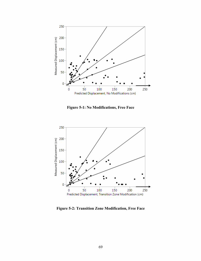
69
Figure 5-1: No Modifications, Free Face
Figure 5-2: Transition Zone Modification, Free Face

70
Figure 5-3: Depth Modification, Free Face
Figure 5-4: Thin Sand Modification, Free Face

71
Figure 5-5: Dilative/Contractive Modification, Free Face
Figure 5-6: Fines Content Modification, Free Face

72
Figure 5-7: Eliminate Thin Sand Modification, Free Face
Figure 5-8: All Modifications, Free Face

73
Figure 5-9: No Modifications, Sloping Ground
Figure 5-10: Transition Zone Modification, Sloping Ground

74
Figure 5-11: Depth Modification, Sloping Ground
Figure 5-12: Thin Sand Modification, Sloping Ground

75
Figure 5-13: Dilative/Contractive Modification, Sloping Ground
Figure 5-14: Fines Content Modification, Sloping Ground

76
Figure 5-15: Eliminate Thin Sand Modification, Sloping Ground
Figure 5-16: All Modifications, Sloping Ground
To visualize the spread and accuracy of the data, simple boundaries are established, similar
to industry convention. Zhang et al. (2004) describes the amount of calculated lateral spread
within, “50 to 200% of measured values.” Using these ranges as a guideline, the following plots

77
display data relative to the 1:1, 2:1, and 0.5:1 lines. These boundary lines help characterize
accuracy of the unmodified and modified predictions. The plots present linear scales up to 250
cm to make the majority of the data more easily viewable. An arrow is used to indicate where
plots have some data off scale. Table 5-1 -- Table 5-3 quantifies the change to the number of data
points that fall in the different ranges with each modification and the all modifications model.
The changes in prediction value assess how the modifications affect the accuracy of the
predictions.
Figure 5-1 -- Figure 5-16 visualize the measured displacement versus predicted
displacement, by ground condition: ground slope (S) or free-face (W). Many individual
soundings improve predictions with the modifications. However, there were also many
soundings where modifications do not improve prediction enough and remains an over
prediction. There were also many soundings where modifications lead to under prediction. To
numerically describe the how the modifications affect the data, Table 5-1, Table 5-2, and Table
5-3 present the amount of data within accuracy categories by modification.
First, accuracy categories were created, using boundaries similar to industry convention.
Certain soundings reduce small predictions minimally, still registering as an under-prediction,
but not extremely variant from the measured displacement. Other soundings are drastically
reduced from extreme predictions to, again, not extremely variant from the measured
displacement. A simple difference of modified results to the measured displacement would
adequately capture small (i.e. <15 cm) prediction improvements as reasonable but curtail
improvements of a larger scale. A simple scalar comparison would identify notable
improvements for all but small numbers, where the prediction may be as different as 10 cm, but
still beyond a factor of two (or half) from the observed displacements. To adequately identify

78
modified soundings as reasonable predictions, both of the above principles are applied. If the
prediction is: 1) within +/-15 cm or 2) within a factor of two of the measured displacement, it is
classified as “Within Reason” (personal communication, Youd and Robertson, 2018). Values
that fall outside that range are classified as “Overpredict” or “Underpredict,” respectively.
Table 5-1 shows how applying different modifications affects prediction accuracy.
Generally, when applying singular or all modifications, the amount of over predictions
decreases, the amount of within reason increases, and the amount of under predictions increases.
Table 5-2 shows the amount of decrease or increase by accuracy category, reinforcing
observations just mentioned.
To go one step further and make observations about how the modifications affect the
accuracy of the predictions for individual accuracy categories, Table 5-3 is provided. This table
separates the data by the starting (no modifications) and ending (after applying modifications)
accuracy categories. This will help highlight how the modifications affect specific accuracy
categories, as the combined results only provides generalized results. It should be noted, due to
the nature of the modifications to only reduce predictions, there is an inherent proclivity to
descend in categories from over predicting to within reason or under predicting, and not the
inverse. Consequently, there are no samples that go from within reason to over predict, from
under predict to over predict, or under predict to within reason. There is also no change in the
amount of samples that start and end in under predict because these modifications only reduce
predictions and under predict is the lowest category. A few observations from Table 5-3 can be
made.

79
Table 5-1: Count of Soundings by Modification and Prediction Accuracy
Table 5-2: Change in Count of Soundings by Modification and Prediction Accuracy
f g y f p y
Accuracy Category
No Modifications
Transition Modification
Depth Modification
Thin Sand Layer
Modification
Dilative/ Contractive Modification
Fines Content
Modification
Elim. Thin Sand Layer Modification
All Modifications
Overpredict 73 72 46 68 64 62 68 17Within Reason 33 30 42 32 34 35 34 56Underpredict 30 34 48 36 38 39 34 63Total 136
g f g y f p y
Accuracy Category
Transition Modification
Depth Modification
Thin Sand Layer
Modification
Dilative/ Contractive Modification
Fines Content
Modification
Elim. Thin Sand Layer Modification
All Modifications
Overpredict -1 -27 -5 -9 -11 -5 -56Within Reason -3 9 -1 1 2 1 23Underpredict 4 18 6 8 9 4 33Note . Negative denotes decrease, positive denotes increase

80
Table 5-3: Count of Data in Each Final Accuracy Category Based on Starting (Unmodified) Accuracy Category
f f y g y g ( f ) y g y
Starting Category
Ending Category
Transition Modification
Depth Modification
Thin Sand Layer
Modification
Dilative/ Contractive Modification
Fines Content
Modification
Elim. Thin Sand Layer Modification
All Modifications
Overpredict Overpredict 72 46 68 64 62 68 17Overpredict Within Reason 1 26 5 9 11 5 47Overpredict Underpredict 0 1 0 0 0 0 9
Within Reason Within Reason 29 16 27 25 24 29 9Within Reason Underpredict 4 17 6 8 9 4 24Underpredict Underpredict 30 30 30 30 30 30 30
Note. 73 start in Overpredict, 33 start in Within Reason, 30 start in Underpredict.

81
The first three rows divide the 73 samples that start in over predict into ending categories
of over predict, within reason, and under predict, based on the modifications applied. The first
row lists the count of soundings that start in over predict and end in over predict. The application
of singular modifications does not drastically reduce this count from 73, aside from the depth
modification. However, applying all modifications does drastically reduce the amount of over
predicting samples from 73 to a mere 17. The second row lists the count of soundings that start
in over predict and end in within reason. The application of singular modifications does not
drastically increase the amount of within reason. However, applying all modifications does place
47 out of the 73 to be within reason. The third row lists the count of soundings that start in over
predict and end in under predict. Applying a singular modification does not increase the amount
of under-predicting samples. However, applying all modifications does generate some under
predictions, 9 out of the 73.
The next two rows divide the 33 samples that start in within reason into ending categories
of within reason and under predict, based on the modifications applied. The first of these rows
lists the count of soundings that start in within reason and end in within reason. The application
of a singular modification doesn’t drastically reduce the count, aside from the depth
modification. However, applying all modifications does drastically reduce the amount of within
reason samples from 33 to 9. The following row lists the count of soundings that start in within
reason and end in under predict. Applying a singular modification only slightly increases the
amount of under-predicting samples, with the exception of the depth modification which
increases greatly. However, applying all modifications greatly increases the amount of under-
predicting samples, 24 of the original 33.

82
There is also the consideration of applying different combinations of modifications.
Without generating all 64 possible combinations, it’s impossible to know the ideal blend of
modifications. Even so, it would only provide an optimum solution for the collection of case
histories used in this study. However, a simpler bypass would be to treat all the modifications as
independent and assess the change in accuracy category for a few combinations. The Depth
Modification is a viable candidate to be considered with another modification because of the
amount of case histories it reduces from over predicting to within reason, 73 to 46. Two other
possible secondary options would be the Dilative/Contractive Modification and the Fines
Content Modification, as they appear to reduce the least amount of predictions that end in
underpredicting, while still increasing the amount of within reason. This approach identifies case
histories in the relevant accuracy category and adds them together, removing possible duplicates.
Duplicates are identified by looking at which case histories are already in the target accuracy
category for both modifications. Two scenarios will be considered: 1) Depth Modification (26
over predict to within reason, 17 within reason to under predict) with Dilative Contractive
Modification (9 over predict to within reason, 8 within reason to under predict) and 2) Depth
Modification with Fines Content Modification (11 over predict to within reason, 9 within reason
to under predict). In the both scenarios, there were equal amounts of common case histories that
went from over prediction to within reason and common case histories that went from within
reason to under prediction. The added benefit of considering another case history would be a
higher amount of cases that are predicted to be within reason, however, this comes at the cost of
also including cases that under predict.
The above observations suggest a few principles. The consistent application of these
modifications to non-clean soil profiles consistently reduces predicted displacements and

83
consistently improves accuracy. These observations also suggest that the implementation of all
modifications to cases of soils where existing methodology performs adequately, significantly
decreases predicted displacements, resulting in potential under prediction. Generally, the
reduction in over prediction comes at the risk of slightly under predicting displacements.
5.1.2 Distribution Charts
The purpose of distribution charts in this study is to assess the accuracy of the data in
reference to the modifications. To quantify accuracy, this analysis describes the difference
between the predicted displacement of the unmodified model and the all modifications applied
model, both relative to the measured displacements. These comparisons establish how different
the model predictions are from the measured field displacements. Using this difference
comparison simplifies the analysis of the modification effectiveness. These distribution charts, or
histograms, visualize the overall trend, and the accompanying box and whisker plots describe the
spread and distribution of the data. The mean is also presented and is a useful indicator for
effectiveness of applied modifications on the overall data, as it represents the center of
distribution. When placed side-by-side, the changes of prediction accuracy by applying all the
modifications become apparent.
The graphics and statistical summary of the distribution charts are presented in Figure 5-17
and Figure 5-18, below. Both parameters are subtracted by the measured displacement, and
labels are condensed on the graph to: “No-dis” (no modifications - displacement) and “All-dis”
(all modifications - displacement). Because the presented values are differences or errors, values
larger than zero indicate over prediction, numbers less than zero indicate under prediction. The
value of bringing the data close to zero establishes a prediction accuracy, where the closer to

84
zero, the more accurate the prediction. This metric is valuable for assessing accuracy for
individual and collective results.
Figure 5-17 and Figure 5-18 allow us to see how different the prediction models compare
to each other in reference to the measured displacement. In both cases, with the free-face and the
ground slope sites, the trends of greatly over-predicted estimates are consistently reduced.
Several clues indicate this pattern. First, the skewed distribution, influenced by over-predicted
data points, becomes more normalized with the application of the modifications as the over
predictions are reduced. Second, the mean value decreases from 140 cm and 182 cm to -9 cm
and -7 cm, respectively. This decrease shows an application of all the modifications presents a
more accurate prediction model, as the all modifications model is significantly closer to zero.
Finally, the box and whisker plots, with a tighter range centered closer to zero, indicate more
accurate predictions for this specific set of case histories. These are strong indicators that
consistent application of the proposed modifications nearly eliminates the potential for gross
over prediction of lateral spread displacements and consistently improves accuracy. This is also
an indicator for the increased potential of slightly under-predicting the displacements.
There are a few possible reasons why this data shows the above-mentioned trends of
reducing over prediction and slightly increasing under prediction. First, the case histories used in
this study contain many non-clean soundings with properties of thin interbedded, transition, or
clayey sand layers. These type of soundings have shown difficulty to accurately predict
displacements (Seed, 1987; Ahmandi & Robertson, 2005; Youd, 2018). These non-clean case
histories represent a large sample of the data used and overall results will reflect a bias in change
in accuracy towards the non-clean soil profiles.

85
Figure 5-17: Distribution Plots, Free-Face (W)

86
Figure 5-18: Distribution Plots, Sloping Ground (S)

87
Another possible reason for the vastly over-predicted values is model extrapolation. For
example, sample 1108 in Christchurch has a free-face W of 4, which is well outside the
recommended bounds of 0.25 to 1. Engineers should interpret extrapolated results with caution,
and application of these proposed modifications does not eliminate or even reduce the risks
associated with extrapolation.
5.1.3 Discriminant Analysis
To further analyze the data, a discriminant analysis was performed to identify
characteristics that might contribute to over-prediction, reasonable prediction, or under-
prediction. A discriminant analysis is used to assess the adequacy of a classification and/or how
effective a certain set of variables are in predicting a category membership. A discriminant
analysis creates canonical variables based on a linear combination of the covariates. Canonical
variables define the two dimensions that provide the maximum separation among the groups.
The plot shows how each covariate contributes to a conical variable. Covariates are standardized
with a mean of 0 and a standard deviation of 1. Ellipses are created to show a 95% confidence
for the categorical variable. Intersecting confidence ellipses indicate an insignificant difference.
The rays denote the covariates, where the length and direction represent the degree of association
to the covariates.
To perform the discriminant analysis, categorical variables and covariates are first defined.
An a priori discrimination is applied to each of the soundings to determine the categorical
variable. The same metric used to classify accuracy categories in section 5.1.1, Regression
Analysis, is used here. If samples are 1) within +/-15 cm or 2) within a factor of two of the
measured displacement, it is classified as “Within Reason.” Values that fall outside that range are

88
classified as “Overpredicted” or “Underpredicted,” respectively. The continuous covariates
available for the deterministic analysis include the PGA, earthquake moment magnitude, and
depth to the water table. The results of the discriminant analysis are presented in Figure 5-19 and
Figure 5-20.
From the discriminant analysis, a few observations and conclusions can be made. First, 25
out of the 74 points corresponding to free-face W sites are misclassified (33%) and only four
within-range soundings are predicted. The discriminant analysis performed accurately and
classifies over half of the free-face sites, but still has a significant amount of uncertainty. The
overlapping ellipses is an indicator that the covariates used would not necessarily distinguish a
sounding as within reason from tending to over-predict or under-predict. However, looking at the
ground slope S data, only 13 out of 62 points, 21%, were misclassified, which is a somewhat
stronger model, but still contains significant uncertainty. For the free-face sites, PGA values vary
and are not within a clean range, although lower values do have some tendency to indicate
under-prediction. Higher PGA values (0.85) are more likely to under-predict with ground slope
sites. High magnitude values (>7.0) tends to be an indicator for over-predicting both free-face
and ground slope sites. Water table depth does not strongly correlate to one specific
classification prediction.
A weakness from interpreting the discriminant data with only the above-listed covariates is
that the modifications discussed in this paper only affect the soil layers and are independent of
the covariates. To perform a more thorough discriminant analysis, more covariates that describe
the soil layers and their properties would be necessary. However, due to the nature of a
discriminant analysis, the soil profile would need to be interpreted and condensed to single-value

89
variables, much like T15 or D5015 used in SPT-based lateral spread analysis, which is beyond the
scope of this study.
Figure 5-19: Discriminant Analysis, Free Face

90
Figure 5-20: Discriminant Analysis, Sloping Ground

91
5.1.4 Results summary
This chapter presents an analysis of the data and sought to answer two main questions. The
first question explores whether the consistent application of these modifications to non-clean
(thin/transition/clayey) soil profiles consistently reduces predicted displacements and
consistently improve accuracy. The regression analysis reveals that a consistent application of
the modifications to non-clean soil profiles does consistently reduce predicted displacements and
consistently improve accuracy. This was evidenced by the decrease in the amount of over
predicting samples and a slight increase in the amount of samples within reason. The distribution
charts also reinforced this idea with the drastic decrease in over predictions. Applying all
modifications shows to be most effective on over-predicting, or non-clean samples. The second
question explores whether the implementation of modifications to cases of soils where existing
methodology perform adequate predictions significantly decrease predicted displacements
resulting in potentially dangerous under prediction. Table 5-3 shows the risk of potentially
dangerous under prediction when all modifications are applied, but there is significantly less of a
risk when only singular modifications are applied. The distribution charts also show the increase
in under prediction with all modifications. The modifications definitely eliminate the potential
for over prediction in interbedded soils, but at the potential risk of under prediction. The
discriminant analysis illustrates that high magnitude values tend to be an indicator for over
prediction and high PGA values tend to be an indicator for over prediction for free-face sites.
It is also useful to note a reduction in prediction from 66 cm to 38 cm, as in Christchurch
15600 with all modifications, may not represent a large shift in displacement because both are
generally considered large displacements. It might be a more concerning possibility if the
modifications predicted no displacements, but more than 15 cm actually occurred. There were

92
approximately 40 sites where applying all modifications reduced the predicted displacement to
below 5 cm, but measured displacement was greater than 15 cm. A majority of those cases were
from one earthquake, Northridge, and a trend isolated to a singular event may can be an
indication of an outlier. The number of sites where the modification reduced displacement
prediction to near zero where the measured displacement was greater than 15 cm drops down to
only 17 sites when considering predicted displacements reduced to below 1 cm. Again, a
majority of those sites were from one case history, Northridge. This risk is further reduced when
considering the application of only singular modifications. All the modifications except the depth
modification lead to few (around or below) 10 scenarios where the predicted displacement was
reduced to below 5 cm and the measured displacement was recorded greater than 15 cm.
Engineers can refer on the discriminant analysis to provide indicators for scenarios like an under
prediction or over prediction. Indicators such as a high PGA as an indicator for gently sloping
ground as tending to under predict. Or a high magnitude as an indicator for over prediction in
free face slope sites.
In summary, application of these modifications reduce over-predictions from strain-based
prediction methods. However, blind or universal application could result in risk of under
prediction. Further research is necessary to determine how to apply these modifications to which
soil conditions. It is also recommended for further research to re-regress a prediction model after
applying these modifications to case histories.

93
6 CONCLUSIONS
Conclusions
This study set out to examine the effectiveness and reliability of six modifications to the
Zhang et al. (2004) CPT-based lateral spread prediction model. These six modifications
included: 1) Soil Transition Zone Modification, 2) Thin Sand Layer Modification, 3)
Dilative/Contractive Modification, 4) Soil Depth Modification, 5) Fines Content Modification,
and 6) Eliminate Thin Sand Modification. Two main questions were considered to evaluate the
modifications. Does the consistent application of these modifications to non-clean
(thin/transition/clayey) soil profiles consistently reduce predicted displacements and consistently
improve accuracy? Does the implementation of modifications to cases of soils where existing
methodology perform adequate predictions significantly decrease predicted displacements
resulting in potentially dangerous under prediction? Several analyses were performed to answer
these questions, including a regression analysis, distribution charts, and a discriminant analysis.
The results showed modifications definitely eliminate the potential for over prediction in
interbedded soils, but at the potential risk of under prediction. Low PGA values are more likely
to under-predict with free-face sites. High PGA values are more likely to under-predict with
gently sloping sites. High moment magnitude values tend to be an indicator for over-predicting
both free-face and gently sloping sites.

94
REFERENCES
(2006, August 18). (U.S. Geological Survey) Retrieved 2019, from About Liquefaction--A cooperative project with the California Geological Survey: https://geomaps.wr.usgs.gov/sfgeo/liquefaction/aboutliq.html#niigata
Ahmandi, M. M., & Robertson, P. K. (2005). Thin-layer effects on the CPT qc measurement. Canadian Geotechnical Journal, 42(5), 1302-1317.
Arduino, S. A., Kramer, S. L., Ilankatharan, M., Kutter, B. L., & Shin, B. L. (2006). Experimental and numerical analysis of seismic soil-pile-structure interaction of a two-span bridge. Proceedings, 8th U.S. National Conference on Earthquake Engineering, Paper No. 504. San Francisco.
Bartlett, S. F., & Youd, T. L. (1992). Empirical analysis of horizontal ground displacement generated by liquefaction-induced lateral spreads. State University of New York. Buffalo, New York: NCEER.
Bartlett, S. F., & Youd, T. L. (1995). Empirical Prediction of Liquefaction-Induced Lateral Spread. Journal of Geotechnical Engineering, 121(4), 316-329.
Bastin, S., Cubrinovski, M., van Ballegooy, S., & Russell, J. (2017). Geologic and geomorphic influences on the spatial extent of lateral spreading in Christchurch, New Zealand. Proc., 3rd Int. Conf. on Performance Based Design in Earthquake Geotechnical Engineering. Vancouver, BC: International Society for Soil Mechanics.
Baziar, M. H., Dobry, R., & Elgamal, A. W. (1992). Engineering evaluation of permanent ground deformations due to seismically-induced liquefaction. Technical Report NCEER-92-0007. Buffalo, New York: National Center for Earthquake Engineering Research, State University of New York.
Bennett, M. J. (1989). Liquefaction analysis of the 1971 ground failure at the San Fernando Valley Juvenile Hall, California. Bulletin of the Association of Engineering Geologists, 26(2), 209-226.
Bennett, M. J., Youd, T. L., Harp, E. L., & Wieczorek, G. F. (1981). Subsurface Investigation of Liquefaction, Imperial Valley Earthquake, California, October 15, 1979. US Geological Survey.
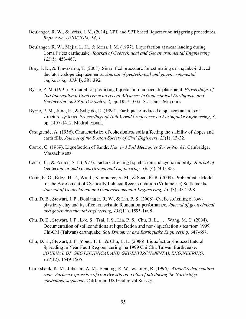
95
Boulanger, R. W., & Idriss, I. M. (2014). CPT and SPT based liquefaction triggering procedures. Report No. UCD/CGM.-14, 1.
Boulanger, R. W., Mejia, L. H., & Idriss, I. M. (1997). Liquefaction at moss landing during Loma Prieta earthquake. Journal of Geotechnical and Geoenvironmental Engineering, 123(5), 453-467.
Bray, J. D., & Travasarou, T. (2007). Simplified procedure for estimating earthquake-induced deviatoric slope displacements. Journal of geotechnical and geoenvironmental engineering, 133(4), 381-392.
Byrne, P. M. (1991). A model for predicting liquefaction induced displacement. Proceedings of 2nd International Conference on recent Advances in Geotechnical Earthquake and Engineering and Soil Dynamics, 2, pp. 1027-1035. St. Louis, Missouri.
Byrne, P. M., Jitno, H., & Salgado, R. (1992). Earthquake-induced displacements of soil-structure systems. Proceedings of 10th World Conference on Earthquake Engineering, 3, pp. 1407-1412. Madrid, Spain.
Casagrande, A. (1936). Characteristics of cohesionless soils affecting the stability of slopes and earth fills. Journal of the Boston Society of Civil Engineers, 23(1), 13-32.
Castro, G. (1969). Liquefaction of Sands. Harvard Soil Mechanics Series No. 81. Cambridge, Massachusetts.
Castro, G., & Poulos, S. J. (1977). Factors affecting liquefaction and cyclic mobility. Journal of Geotechnical and Geoenvironmental Engineering, 103(6), 501-506.
Cetin, K. O., Bilge, H. T., Wu, J., Kammerer, A. M., & Seed, R. B. (2009). Probabilistic Model for the Assessment of Cyclically Induced Reconsolidation (Volumetric) Settlements. Journal of Geotechnical and Geoenvironmental Engineering, 135(3), 387-398.
Chu, D. B., Stewart, J. P., Boulanger, R. W., & Lin, P. S. (2008). Cyclic softening of low-plasticity clay and its effect on seismic foundation performance. Journal of geotechnical and geoenvironmental engineering, 134(11), 1595-1608.
Chu, D. B., Stewart, J. P., Lee, S., Tsai, J. S., Lin, P. S., Chu, B. L., . . . Wang, M. C. (2004). Documentation of soil conditions at liquefaction and non-liquefaction sites from 1999 Chi-Chi (Taiwan) earthquake. Soil Dynamics and Earthquake Engineering, 647-657.
Chu, D. B., Stewart, J. P., Youd, T. L., & Chu, B. L. (2006). Liquefaction-Induced Lateral Spreading in Near-Fault Regions during the 1999 Chi-Chi, Taiwan Earthquake. JOURNAL OF GEOTECHNICAL AND GEOENVIRONMENTAL ENGINEERING, 132(12), 1549-1565.
Cruikshank, K. M., Johnson, A. M., Fleming, R. W., & Jones, R. (1996). Winnetka deformation zone: Surface expression of coactive slip on a blind fault during the Northridge earthquake sequence. California: US Geological Survey.

96
DeDen, D. W. (2004). Analysis of lateral spreads generated by the 1999 Kocaeli, Turkey earthquake. Master of Science Thesis, Brigham Young University, Department of Civil and Environmental Engineering.
Deterling, O. C. (2015). Factors Influencing the Lateral Spread Displacement from the 2011 Christchurch, New Zealand Earthquake. Masters of Science in Engineering, The University of Texas at Austin.
Dobry, R., & Baziar, M. H. (1991). Evaluation of ground deformation caused by lateral spreading. 3rd- Japan-U.S. Workshop on Earthquake Resistant Design of Lifeline Facilities and Countermeasures for Soil Liquefaction (pp. 209-223). NCEER-91-0001.
Dobry, R., Ladd, R. S., Yokel, F. Y., Chang, R. M., & Powell, D. (1982). Prediction of pore water pressure buildup and liquefaction of sands during earthquakes by the cyclic strain method (Vol. 138). Gaithersburg, MD: National Bureau of Standards.
Dobry, R., Thevanayagam, S., Medina, C., Bethapudi, R., Elgamal, A., Bennett, V., . . . Mercado, V. M. (2011, February). Mechanics of Lateral Spreading Observed in a Full-Scale Shake Test. Journal of Geotechnical and Geoenvironmental engineering, 137(2), 115-129.
Earthquake Commission. (n.d.). Retrieved 2017, from New Zealand Geotechnical Database: www.nzgd.org.nz
Finn, W. D., Yogendrakumar, M., Yoshida, M., & Yoshida, N. (1986). TARA-3: A program to compute the response of 2-D embankments and soil-structure interaction systems to seismic loadings. Vancouver, British Columbia: Department of Civil Engineering, University of British Columbia.
Franke, K. W., Blonquist, J. L., He, J., Hatch, M., Coutu, T., & Arndt, A. (2019). CPTLiquefY: A New Research Tool for Performance-Based Liquefaction Hazard Assessment using the CPT.
GeoLogismiki. (n.d.). CLiq-CPT soil liquefaction software. v.3.0. Retrieved from https://geologismiki.gr/products/cliq/
Gu, W. H., Morgenstern, N. R., & Robertson, P. K. (1994). Post-earthquake deformation analysis of wildlife sites. Journal of Geotechnical Engineering, 120(2), 274-289.
Hadush, S., Yashima, A., Uzuoka, R., Moriguchi, S., & Sawada, K. (2001). Liquefaction induced lateral spread analysis using the CIP method. Computers and Geotechnics, 28(8), 549-574.
Hamada, M., Towhata, I., Yasuda, S., & Isoyama, R. (1987). Study on permanent ground displacement induced by seismic liquefaction. Computers and Geotechnics, 4(4), 197-220.
97
Hamada, M., Yasuda, S., Isoyama, R., & Emoto, K. (1986). Study on liquefaction induced permanent ground displacements. Association for the development of Earthquake Prediction.
Hamada, M., Yasuda, S., Isoyama, R., & Emoto, K. (1986). Study on liquefaction induced permanent ground displacements. Report for Association for the Development of Earthquake Prediction.
Hanzawa, H., Yutaka, I., & Kazuyuki, S. (1979). Shear characteristics of a quick sand in the Arabian Gulf. Soils and Foundations, 19(4), 1-15.
Holzer, T. L., Bennett, M. J., Ponti, D. J., & Tinsley III, J. C. (1999). Liquefaction and soil failure during 1994 Northridge earthquake. Journal of Geotechnical and Geoenvironmental Engineering, 125(6), 438-452.
Holzer, T. L., Bennett, M. J., Tinsley, J. C., Ponti, D. J., & Sharp, R. V. (1996). Causes of ground failure in alluvium during the Northridge, California, earthquake of January 17, 1994. Japan-US Workshop on Earthquake Resistant Design of Lifeline Facilities and Countermeasures Against Soil Liquefaction. 6, pp. 345-60. US National Center for Earthquake Engineering Research.
Ishihara, K. (1984). Post-earthquake failure of a tailings dam due to liquefaction of pond deposit. Proceedings of International Conference on Case Histories in Geotechnical Engineering,, (pp. 1129-1143).
Ishihara, K. (1985). Stability of natural deposits during earthquakes. Proceedings of 11th ICSMFE, 1985, (pp. 321-376).
Ishihara, K., & Yoshimine, M. (1992). Evaluation of settlements in sand deposits following liquefaction during earthquakes. Soils and foundations, 32(1), 173-188.
Iwasaki, T. T. (1982). Microzonation for soil liquefaction potential using simplified methods. roceedings of the 3rd international conference on microzonation, (pp. 1310-1330). Seattle.
Jefferies, M. G., & Been, K. (2006). Soil Liquefaction - A critical state approach.
Jefferies, M. G., & Davies, M. P. (1993). Use of CPTU to estimate equivalent SPT N 60. Geotechnical Testing Journal, 16(4), 458-468.
Johnson, A. M., Fleming, R., Cruikshank, K. M., & Packard, R. F. (1996). Coactive fault of the Northridge earthquake—Granada Hills area, California. U. S. Geological Survey(96-253).
Joyner, W. B., & Boore, D. M. (1981). Peak horizontal acceleration and velocity from strong-motion records including records from the 1979 Imperial Valley, California, earthquake. Bulletin of the Seismological Society of America, 71(6), 2011-2038.
Kayen, R. E., Mitchell, J. K., Seed, R. B., Lodge, A., Nishio, S., & Cotinho, R. (1992). Evaluation of SPT-, CPT-, and shear wave-based methods for liquefaction potential

98
assessment using Loma Prieta data. Proceedings, 4th U.S.-Japan Workshop on Earthquake Resistant Design of Lifeline Facilities and Countermeasures for Soil Liquefaction, 1, pp. 177-204.
Kramer, S. L. (1996). Geotechnical Earthquake Engineering. Upper Saddle River, New Jersey: Prentice Hall, Inc.
Middlebrooks, T. A. (1942). Fort Peck Slide. Transactions of the American Society of Civil Engineers, 107(1), 723-742.
Mohamad, R., & Dobry, R. (1986). Undrained monotonic and cyclic triaxial strength of sand. Journal of Geotechnical Engineering, 112(10), 941-958.
Nagase, H., & Ishihara, K. (1988). Liquefaction-induced compaction and settlement of sand during earthquakes. Soils Foundations, 28(1), 65-76.
Newmark, N. M. (1965). Effects of earthquakes on dams and embankments. Geotechnique, 15(2), 139-160.
Niekerken, B. V. (2018, April 18). 1906 San Francisco earthquake: Old photos offer new glimpses of devastation.
Page, R. A., Stauffer, P. H., & Hendley II, J. W. (1999, May 6). Progress Toward a Safer Future Sinc ethe 1989 Loma Prieta Earthquake. Retrieved from U.S. Geological Survey: https://pubs.usgs.gov/fs/1999/fs151-99/
Poulos, S. J. (1981). The steady state of deformation. Journal of Geotechnical and Geoenvironmental Engineering, 107(GT5), 553-562.
Quigley, M. C., Bastin, S., & Bradley, B. A. (2013). Recurrent liquefaction in Christchurch, New Zealand, during the Canterbury earthquake sequence. Geology, 41(4), 419-422.
Rauch, A. F. (1997). EPOLLS: an empirical method for prediciting surface displacements due to liquefaction-induced lateral spreading in earthquakes. Doctoral Dissertation, Virginia Tech.
Robertson, P. K. (1990). Soil classification using the cone penetration test. Canadian Geotechnical Journal, 27(1), 151-158.
Robertson, P. K. (2009). Interpretation of cone penetration tests—a unified approach. Canadian geotechnical journal, 46(11), 1337-1355.
Robertson, P. K. (2009). Performance based earthquake design using the CPT. In Kokusho, Tsukamoto, & Yoshimine (Ed.), Performance-Based Design in Earthquake Geotechnical Engineering (pp. 3-20). Tokyo: Taylor & Francis Group.
Robertson, P. K. (2010). Evaluation of flow liquefaction and liquefied strength using the cone penetration test. Journal of Geotechnical and Geoenvironmental Engineering, 136(6), 842-853.

99
Robertson, P. K. (2011). Computing in Geotechnical Engineering-Automatic Software Detection of CPT Transition Zones. Geotechnical News, 29(2), 35-38.
Robertson, P. K., & Wride, C. E. (1998). Evaluating cyclic liquefaction potential using the cone penetration test. Canadian Geotechnical Journal, 35(3), 442-459.
Ross, G. A., Seed, H. B., & Migliaccio, R. R. (1969). Bridge foundation behavior in Alaska earthquake. Journal of the Soil Mechanics and Foundations Division, 95(4), 1007-1036.
Sasaki, Y., Tokida, K., Matsumoto, H., & Saya, Y. (1991). Shake table tests on lateral ground flow induced by soil liquefaction. In T. D. O'Rourke, & M. Hamada (Ed.), 3rd Japan-U.S. Workshop on Earthquake Resistant Design of Lifeline Facilities and Countermeasures for Soil Liquefaction (pp. 371-385). Buffalo, N.Y.: National Center for Earthquake Engineering Research, SUNY-Buffalo.
Saygili, G., & Rathje, E. M. (2008). Empirical predictive models for earthquake-induced sliding displacements of slopes. Journal of Geotechnical and Geoenvironmental Engineering, 134(6), 790-803.
Seed, H. B. (1979). Soil liquefaction and cyclic mobility evalution for level ground during earthquakes. Journal of geotechnical and geoenvironmental engineering, 105(GT2), 201-225.
Seed, H. B., & Idriss, I. M. (1971). Simplified procedure for evaluating soil liquefaction potential. Journal of Soil Mechanics & Foundations Div., 1249-1273.
Seed, H. B., & Idriss, I. M. (1982). Ground motions and soil liquefaction during earthquakes. Earthquake engineering research insititue, 134.
Seed, R. B., Dickenson, S. E., & Idriss, I. M. (1991, March). Principal Geotechnical Aspects of the 1989 Loma Prieta Earthquake. Soils and Foudnations, 31, 1-26.
Shiomi, T., Tsukuni, S., Hatanaka, M., Tanaka, Y., Suzuki, Y., & Hirose, T. (1987). Simulation analysis of ground liquefaction induced by earthquake. Computers and Geotechnics, 4(4), 221-245.
Stewart, J. P., Seed, R. B., & Bray, J. D. (1996). Incidents of ground failure from the 1994 Northridge earthquake. Bulletin of the Seismological Society of America, 86(1B), S300-S318.
Taboada, V. M., Abdoun, T., & Dobry, R. (1996). Prediction of liquefaction-induced lateral spreading by dilatant sliding block model calibrated by centrifuge tests. Proceedings of 11th World Conference on Earthquake Engineering. Oxford, UK: Pergamon.
Taboada-Urtuzuastegui, V. M., & Dobry, R. (1998). Centrifuge modeling of earthquake-induced lateral spreading in sand. Journal of Geotechnical and Geoenvironmental Engineering, 124(12), 1195-1206.

100
Tatsuoka, F., Zhou, S., Sato, T., & Shibuya, S. (1990). Method of evaluating liquefaction potential and its application. Ministry of Education of Japan.
Towhata, I., Sasaki, Y., Tokida, K., MATSUMOTO, H., TAMARI, Y., & Yamada, K. (1992). Prediction of permanent displacement of liquefied ground by means of minimum energy principle. Soils and Foundations, 32(3), 97-116.
Towhata, I., Tokida, K., Tamari, Y., Matsumoto, H., & Yamada, K. (1991). Prediction of permanent lateral displacement of liquefied ground by means of variational principle. In T. D. O'Rourke, & M. Hamada (Ed.), Proceedings of the 3rd Japan–US workshop on earthquake resistant design of lifeline facilities and countermeasures for soil liquefaction (pp. 237-251). New York: NCEER-91-0001.
Treadwell, D. D. (1976). The Influence of Gravity, Prestess, Compressibility, and Layering on Soil Resistance to Static Penetration. PhD Thesis, University of California at Berkeley, Berkeley, California.
Vaid, Y. P., Chung, E. K., & Kuerbis, R. H. (1990). Stress path and steady state. Canadian Geotechnical Journal, 27(1), 1-7.
Valsamis, A. I., Bouckovalas, G. D., & Papadimitrou, A. G. (2010). Parametric investigation of lateral spreading of gently sloping liquefied ground. Soil Dynamics and Earthquake Engineering, 30(6), 490-508.
Yang, Z. (2000). Numerical modeling of earthquake site response including dilation and liquefaction. PhD Dissertation, Columbia University, New York City.
Yang, Z., Elgamal, A., & Parra, E. (2003). A computational model for liquefaction and associated shear deformation. Journal of Geotechnical and Geoenvironmental Engineering, 129(12), 1119-1127.
Yasuda, S., Nagase, H., KIKU, H., & UCHIDA, Y. (1992). The mechanism and a simplified procedure for the analysis of permanent ground displacement due to liquefaction. Soils and Foundations, 32(1), 149-160.
Youd, T. L. (1984). Recurrence of liquefaction at the same site. Proceedings 8th World Conference Earthquake Engineering. 3, pp. 231-238. Prentice-Hall Inc.
Youd, T. L. (2018). Application of MLR Procedure for Prediction of Liquefaction-Induced Lateral Spread Displacement. Journal of Geotechnical and Geoenvironmental Engineering, 144(6), 04018033.
Youd, T. L., & Hoose, S. N. (1977). Liquefaction susceptibility and geologic setting. Proceedings, 6th World Conference on Earthquake Engineering, 3, pp. 2189-2194. New Delhi.
Youd, T. L., & Hoose, S. N. (1978). Historic ground failures in Northern California triggered by earthquakes. U.S. Geological Survey(Professional Paper 993).

101
Youd, T. L., & Idriss, I. M. (2001). Liquefaction resistance of soils: Summary report from the 1996 NCEER and 1998 NCEER/NSF workshops on evaluation of liquefaction resistance of soils. Journal of Geotechnical and Geoenvironmental Engineering, 127(10), 817-833.
Youd, T. L., & Perkins, D. M. (1987). Mapping of liquefaction severity index. Journal of Geotechnical Engineering, 113(11), 1374-1392.
Youd, T. L., DeDen, D. W., Bray, J. D., Sancio, R., Cetin, K. O., & Gerber, T. M. (2009). Zero-displacement lateral spreads. 1999 Kocaeli, Turkey earthquake. Journal of Geotechnical and Geoenvironmental Engineering, 135(1), 46-61.
Youd, T. L., Hansen, C. M., & Bartlett, S. F. (1999). Revised MLR equations for predicting lateral spread displacement. Proc. 7th US–Japan Workshop on Earthquake Resistant Design of Lifeline Facilities and Countermeasures Against Liquefaction. 19, pp. 99-114. Seattle: Tech. Rep. No. MCEER-99.
Youd, T. L., Hansen, C. M., & Bartlett, S. F. (2002). Revised multilinear regression equations for prediction of lateral spread displacement. Journal of Geotechnical and Geoenvironmental Engineering, 128(12), 1007-1017.
Zhang, G., Robertson, P. K., & Brachman, R. W. (2002). Estimating liquefaction-induced ground settlements from CPT for level ground. Canadian Geotechnical Journal, 39(5), 1168-1180.
Zhang, G., Robertson, P. K., & Brachman, R. W. (2004). Estimating liquefaction-induced lateral displacements using the standard penetration test or cone penetration test. Journal of Geotechnical and Geoenvironmental Engineering, 130(8), 861-871.
Zhang, J. M., & Wang, G. (2012). Large post-liquefaction deformation of sand, part I: physical mechanism, constitutive description, and numerical algorithm. Acta Geotechnica, 7(2), 69-113.
Zienkiewics, O. C., & Shiomi, T. (1984). Dynamic behavior of saturated porous media: the. International Journal for Numerical and Analytical Methods in Geomechancis(8), 71-96.
Zienkiewics, O. C., Chang, C. T., & Hinton, E. (1978). Non-linear seismic response and liquefaction. International Journal for Numerical and Analytical Methods in Geomechanics(2), 381-404.
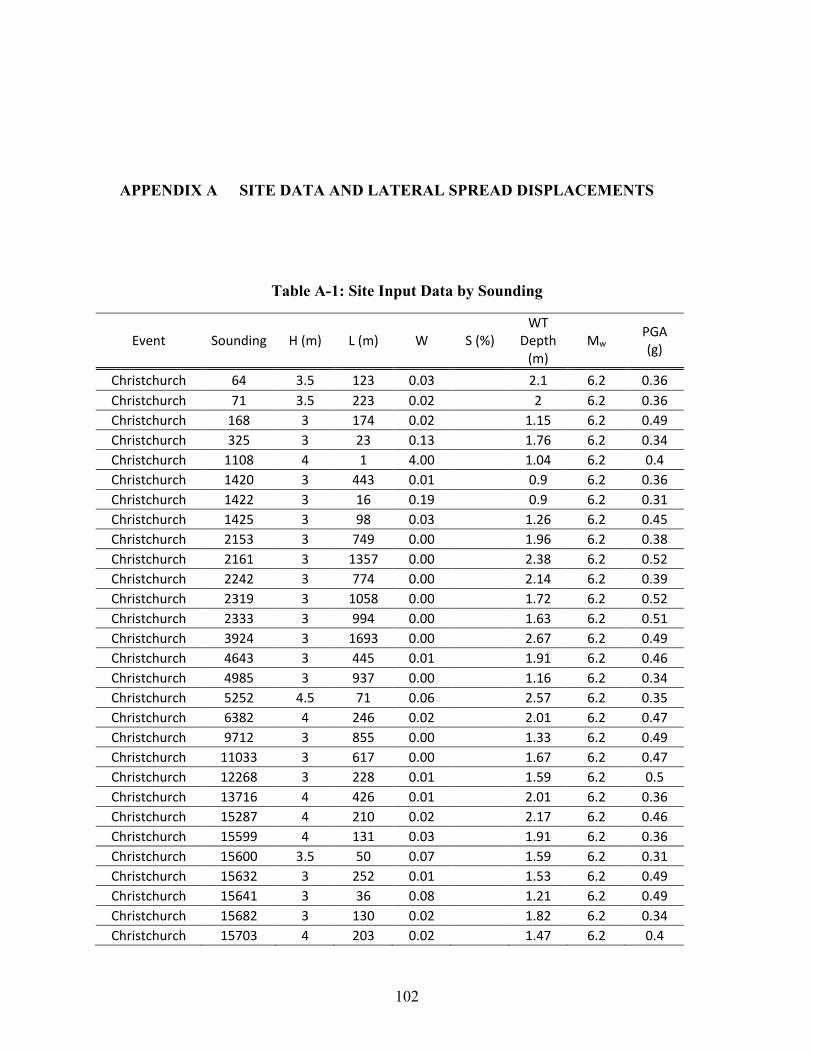
102
APPENDIX A SITE DATA AND LATERAL SPREAD DISPLACEMENTS
Table A-1: Site Input Data by Sounding
Event Sounding H (m) L (m) W S (%) WT
Depth (m)
Mw PGA (g)
Christchurch 64 3.5 123 0.03 2.1 6.2 0.36 Christchurch 71 3.5 223 0.02 2 6.2 0.36 Christchurch 168 3 174 0.02 1.15 6.2 0.49 Christchurch 325 3 23 0.13 1.76 6.2 0.34 Christchurch 1108 4 1 4.00 1.04 6.2 0.4 Christchurch 1420 3 443 0.01 0.9 6.2 0.36 Christchurch 1422 3 16 0.19 0.9 6.2 0.31 Christchurch 1425 3 98 0.03 1.26 6.2 0.45 Christchurch 2153 3 749 0.00 1.96 6.2 0.38 Christchurch 2161 3 1357 0.00 2.38 6.2 0.52 Christchurch 2242 3 774 0.00 2.14 6.2 0.39 Christchurch 2319 3 1058 0.00 1.72 6.2 0.52 Christchurch 2333 3 994 0.00 1.63 6.2 0.51 Christchurch 3924 3 1693 0.00 2.67 6.2 0.49 Christchurch 4643 3 445 0.01 1.91 6.2 0.46 Christchurch 4985 3 937 0.00 1.16 6.2 0.34 Christchurch 5252 4.5 71 0.06 2.57 6.2 0.35 Christchurch 6382 4 246 0.02 2.01 6.2 0.47 Christchurch 9712 3 855 0.00 1.33 6.2 0.49 Christchurch 11033 3 617 0.00 1.67 6.2 0.47 Christchurch 12268 3 228 0.01 1.59 6.2 0.5 Christchurch 13716 4 426 0.01 2.01 6.2 0.36 Christchurch 15287 4 210 0.02 2.17 6.2 0.46 Christchurch 15599 4 131 0.03 1.91 6.2 0.36 Christchurch 15600 3.5 50 0.07 1.59 6.2 0.31 Christchurch 15632 3 252 0.01 1.53 6.2 0.49 Christchurch 15641 3 36 0.08 1.21 6.2 0.49 Christchurch 15682 3 130 0.02 1.82 6.2 0.34 Christchurch 15703 4 203 0.02 1.47 6.2 0.4

103
Table A-1 Continued
Event Sounding H (m) L (m) W S (%) WT
Depth (m)
Mw PGA (g)
Christchurch 15772 3 35 0.09 1.43 6.2 0.5 Christchurch 15776 3 132 0.02 0.87 6.2 0.33 Christchurch 19088 3.5 273 0.01 1.85 6.2 0.33 Christchurch 21509 4 50 0.08 1.85 6.2 0.4 Christchurch 21510 4 27 0.15 1.77 6.2 0.4 Christchurch 26641 4 315 0.01 2.11 6.2 0.4 Christchurch 27046 3 1548 0.00 2.47 6.2 0.51 Christchurch 29053 4 46 0.09 1.82 6.2 0.36 Christchurch 29058 4 71 0.06 1.97 6.2 0.36 Christchurch 34460 4 95 0.04 2.08 6.2 0.4 Christchurch 34616 3 713 0.00 3.23 6.2 0.34 Christchurch 38115 3 289 0.01 1.83 6.2 0.45 Christchurch 38121 3 351 0.01 1.9 6.2 0.34
Imperial Valley 442 1.56 26 0.06 1.8 6.6 0.7
Imperial Valley 700-lsu006 1.56 27.67 0.06 1.8 6.6 0.7
Imperial Valley Heber 1 2 4.5 0.44 1.75 6.6 0.6 Imperial Valley Heber 2 2 4.5 0.44 1.75 6.6 0.6 Imperial Valley Heber 3 2 4.5 0.44 1.75 6.6 0.6 Imperial Valley Heber 4 2 4.5 0.44 1.75 6.6 0.6 Imperial Valley Heber 5 2 4.5 0.44 1.75 6.6 0.6 Imperial Valley Heber 6 2 4.5 0.44 1.75 6.6 0.6 Imperial Valley Heber 7 2 4.5 0.44 1.75 6.6 0.6 Imperial Valley Heber 8 2 4.5 0.44 1.75 6.6 0.6 Imperial Valley pqs1 0.40% 0 6.6 0.2 Imperial Valley pqs2 0.40% 0 6.6 0.2 Imperial Valley pqs3 0.40% 0 6.6 0.2 Imperial Valley pqs4 0.40% 0 6.6 0.2 Imperial Valley pqs5 0.40% 0 6.6 0.2
Loma Prieta UC-18 3.7 26 0.14 3.4 7 0.25 Loma Prieta UC-2 5.4 28.3 0.19 1.7 7 0.25 Loma Prieta UC-3 5.5 14.7 0.37 1.7 7 0.25 Loma Prieta UC-4 5.3 30.5 0.18 1.8 7 0.25 Loma Prieta UC-5 5.2 18.7 0.28 1.8 7 0.25 Loma Prieta UC-6 5.1 35.6 0.14 1.7 7 0.25 Northridge BAL-1 0.70% 10.7 6.7 0.85 Northridge BAL-10 0.70% 7.3 6.7 0.85 Northridge BAL-11 0.70% 7.8 6.7 0.85 Northridge BAL-12 0.70% 7.7 6.7 0.85

104
Table A-1 Continued
Event Sounding H (m) L (m) W S (%) WT
Depth (m)
Mw PGA (g)
Northridge BAL-13 0.70% 8.2 6.7 0.85 Northridge BAL-13.5 0.70% 8.4 6.7 0.85 Northridge BAL-15 0.70% 10.7 6.7 0.85 Northridge BAL-16 0.70% 17.1 6.7 0.85 Northridge BAL-2 0.70% 9.45 6.7 0.85 Northridge BAL-3 0.70% 9 6.7 0.85 Northridge BAL-4 0.70% 8.7 6.7 0.85 Northridge BAL-5 0.70% 8.4 6.7 0.85 Northridge BAL-6 0.70% 8.3 6.7 0.85 Northridge BAL-7 0.70% 8.2 6.7 0.85 Northridge BAL-8 0.70% 8.1 6.7 0.85 Northridge BAL-9 0.70% 7.7 6.7 0.85 Northridge MAL-11 0.70% 3.9 6.7 0.51 Northridge MAL-12 0.70% 3.9 6.7 0.51 Northridge MAL-13 0.70% 3.9 6.7 0.51 Northridge MAL-3 0.70% 3.9 6.7 0.51 Northridge MAL-4 0.70% 3.9 6.7 0.51 Northridge MAL-5 0.70% 3.9 6.7 0.51 Northridge POT-1 2.70% 5.6 6.7 0.43 Northridge POT-10 2.70% 2.6 6.7 0.43 Northridge POT-11 2.70% 2.2 6.7 0.43 Northridge POT-12 2.70% 2 6.7 0.43 Northridge POT-3 0.70% 3.2 6.7 0.43 Northridge POT-4 0.70% 2.7 6.7 0.43 Northridge POT-5 0.70% 2.9 6.7 0.43 Northridge POT-6 0.70% 2.8 6.7 0.43 Northridge POT-7 0.70% 2.5 6.7 0.43 Northridge POT-8 2.70% 3.3 6.7 0.43 Northridge POT-9 2.70% 2.6 6.7 0.43 Northridge WYN-1 1.80% 4.8 6.7 0.51 Northridge WYN-10 1.80% 4.2 6.7 0.51 Northridge WYN-11 1.80% 4.3 6.7 0.51 Northridge WYN-12 0.30% 3.9 6.7 0.51 Northridge WYN-13 0.30% 4.3 6.7 0.51 Northridge WYN-14 1.50% 6.7 6.7 0.51 Northridge WYN-2 1.80% 4.4 6.7 0.51 Northridge WYN-3 1.80% 4.4 6.7 0.51 Northridge WYN-4 1.80% 4.3 6.7 0.51

105
Table A-1 Continued
Event Sounding H (m) L (m) W S (%) WT
Depth (m)
Mw PGA (g)
Northridge WYN-5 1.80% 4.3 6.7 0.51 Northridge WYN-7 1.80% 3.8 6.7 0.51 Northridge WYN-8 1.10% 4 6.7 0.51
San Fernando sfvjh81-2 0.80% 3.3 6.4 0.5 San Fernando sfvjh81-4 0.80% 3.3 6.4 0.5 San Fernando sfvjh81-6 0.80% 3.3 6.4 0.5 San Fernando sfvjh9 0.80% 3.3 6.4 0.5
Taiwan MAA-C-9 3 24.5 0.12 1 7.6 0.67 Taiwan NCC-2 3.80% 5.3 7.6 0.39 Taiwan NCC-3 3.80% 1.5 7.6 0.39 Taiwan RESI-C7 2.9 4 0.73 1.245 7.6 0.67 Taiwan WBC-1 2.9 46 0.06 1.122 7.6 0.67 Taiwan WBC-4 2.9 15.3 0.19 1.288 7.6 0.67 Taiwan WCC-1 2.9 11.8 0.25 1.245 7.6 0.67 Taiwan WCC-11 2.8 53.5 0.05 1.33 7.6 0.67 Taiwan WCC-12 3 18.5 0.08 0.75 7.6 0.67 Taiwan WCC-13 2.9 58.4 0.04 0.9 7.6 0.67 Taiwan WCC-2 2.9 23.8 0.12 1.254 7.6 0.67 Taiwan WCC-4 2.8 15 0.19 1.24 7.6 0.67 Taiwan WCC-6 3.5 26.5 0.13 1.11 7.6 0.67 Taiwan WCC-7 3.5 37.5 0.09 1.1 7.6 0.67 Taiwan WCC-8 2.8 40 0.07 1.2 7.6 0.67 Taiwan WCC-9 3.5 18.5 0.19 1.12 7.6 0.67 Turkey Cark 24 3.5 15 0.23 2.601 7.4 0.41 Turkey Cark 25 3.5 15 0.23 2.6 7.4 0.41 Turkey dn1 20.00% 1.7 7.4 0.3 Turkey dn2 20.00% 2.5 7.4 0.3 Turkey dn3 20.00% 1.7 7.4 0.3
Turkey Cumhuriyet 22 0.30% 0.951 7.4 0.41
Turkey Cumhuriyet 23 0.30% 1.699 7.4 0.41
Turkey Cumhuriyet 24 0.30% 1.265 7.4 0.41

106
Table A-2: Measured and Predicted Lateral Spread Displacements by Modifications and Sounding
Event Sounding Measured Disp. (cm)
Predicted Disp., No
Mod. (cm)
Predicted Disp.,
Transition (cm)
Predicted Disp., Depth (cm)
Predicted Disp., Thin Sand
(0.3m) (cm)
Predicted Disp.,
Dil/Cont (cm)
Predicted Disp., Fines
Content (cm)
Predicted Disp.,
Elim Thin Sand
(0.3m) (cm)
Predicted Disp., All
Mod. (cm)
Christchurch 64 4 77.4 71.4 43.1 71.6 55.2 67.8 71.6 18.1 Christchurch 71 4 47.9 43.6 13.9 46.8 41.0 44.2 46.8 11.9 Christchurch 168 28 127.9 122.7 38.7 122.6 79.4 116.7 122.6 12.0 Christchurch 325 89 147.0 134.9 97.8 147.0 100.7 145.3 147.0 54.0 Christchurch 1108 79 3594.6 3338.2 2195.0 3363.9 3098.9 3234.5 3363.8 1640.8 Christchurch 1420 77 24.1 22.5 15.5 23.3 13.6 19.5 23.3 7.3 Christchurch 1422 87 302.2 285.9 218.8 279.0 157.0 285.1 278.9 63.1 Christchurch 1425 62 60.4 56.2 49.9 57.5 25.8 46.5 57.5 13.1 Christchurch 2153 18 7.1 6.7 1.8 7.1 7.1 7.0 7.1 1.5 Christchurch 2161 48 7.7 7.6 2.8 7.7 6.3 7.6 7.7 1.3 Christchurch 2242 29 9.0 8.1 5.0 9.0 6.8 8.3 9.0 2.1 Christchurch 2319 90 7.6 7.2 3.4 7.6 6.6 7.0 7.6 2.0 Christchurch 2333 83 6.5 6.3 2.9 6.5 6.2 6.5 6.5 2.6 Christchurch 3924 39 2.6 2.5 0.9 2.6 2.1 2.5 2.6 0.3 Christchurch 4643 32 15.2 14.5 9.7 13.4 11.5 13.9 13.4 6.0 Christchurch 4985 36 6.5 5.8 2.3 6.5 5.6 6.0 6.5 1.5 Christchurch 5252 38 75.8 71.5 42.2 73.8 35.9 64.0 73.8 6.3 Christchurch 6382 6 15.1 14.3 6.7 15.1 15.1 15.1 15.1 6.2 Christchurch 9712 84 4.5 4.2 1.4 3.9 4.5 4.2 3.9 1.2 Christchurch 11033 60 14.6 14.1 8.5 14.6 7.2 14.2 14.6 1.3 Christchurch 12268 66 21.5 20.5 0.6 21.5 21.5 21.4 21.5 0.3 Christchurch 13716 0.1 4.0 3.8 1.3 4.0 4.0 4.0 4.0 1.3

107
Table A-2 Continued
Event Sounding Measured Disp. (cm)
Predicted Disp., No
Mod. (cm)
Predicted Disp.,
Transition (cm)
Predicted Disp., Depth (cm)
Predicted Disp., Thin Sand
(0.3m) (cm)
Predicted Disp.,
Dil/Cont (cm)
Predicted Disp., Fines
Content (cm)
Predicted Disp.,
Elim Thin Sand
(0.3m) (cm)
Predicted Disp., All
Mod. (cm)
Christchurch 15287 27 6.9 6.6 3.9 6.9 6.9 6.7 6.9 3.7 Christchurch 15599 76 13.9 12.7 10.8 13.9 12.9 13.5 13.9 8.9 Christchurch 15600 95 66.0 58.9 58.0 66.0 50.9 62.6 66.0 37.5 Christchurch 15632 10 10.0 9.3 8.1 10.0 6.7 10.0 10.0 4.6 Christchurch 15641 93 50.3 45.8 34.3 43.0 32.9 45.7 43.0 12.8 Christchurch 15682 52 26.8 26.0 18.9 26.1 15.4 24.0 26.1 7.8 Christchurch 15703 35 19.3 18.4 19.3 19.3 8.4 19.3 19.3 8.9 Christchurch 15772 105 60.7 56.7 51.3 60.7 36.7 56.9 60.7 30.1 Christchurch 15776 90 45.8 42.5 35.0 40.6 35.3 39.6 40.6 16.7 Christchurch 19088 9 2.5 2.5 1.7 2.5 2.5 2.5 2.5 1.6 Christchurch 21509 69 89.9 83.6 33.6 89.9 77.3 89.9 89.9 19.8 Christchurch 21510 106 141.2 129.6 49.7 141.2 134.6 132.2 141.2 38.8 Christchurch 26641 21 34.6 31.4 22.1 33.7 29.6 33.2 33.7 16.3 Christchurch 27046 43 3.9 3.7 2.5 3.8 3.5 3.6 3.8 1.8 Christchurch 29053 104 82.3 79.5 77.7 82.3 41.7 81.1 82.3 37.6 Christchurch 29058 102 83.1 78.8 68.7 83.1 61.4 75.1 83.1 49.0 Christchurch 34460 57 23.8 22.6 14.9 23.8 23.8 22.9 23.8 14.6 Christchurch 34616 38 9.5 8.7 5.5 8.9 5.2 8.5 8.9 1.9 Christchurch 38115 39 10.6 9.9 6.5 8.4 7.9 10.6 8.4 3.4 Christchurch 38121 69 0.1 0.1 0.1 0.1 0.1 0.1 0.1 0.1
Imperial Valley 442 100 90.9 90.8 16.6 64.1 81.7 56.5 64.1 7.1
Imperial Valley 700-lsu006 100 125.2 122.3 27.5 110.5 119.3 98.7 110.5 19.3
Imperial Valley Heber 1 120 36.7 36.7 0.1 36.7 36.7 6.8 36.7 0.1

108
Table A-2 Continued
Event Sounding Measured Disp. (cm)
Predicted Disp., No
Mod. (cm)
Predicted Disp.,
Transition (cm)
Predicted Disp., Depth (cm)
Predicted Disp., Thin Sand
(0.3m) (cm)
Predicted Disp.,
Dil/Cont (cm)
Predicted Disp., Fines
Content (cm)
Predicted Disp.,
Elim Thin Sand
(0.3m) (cm)
Predicted Disp., All
Mod. (cm)
Imperial Valley Heber 2 120 358.8 347.9 123.5 326.6 283.7 153.3 326.6 54.6 Imperial Valley Heber 3 120 290.1 290.1 155.5 225.9 225.9 142.4 225.9 68.0 Imperial Valley Heber 4 120 557.8 557.8 285.7 409.6 493.5 194.3 409.4 108.6 Imperial Valley Heber 5 120 322.2 322.2 193.4 258.0 290.1 73.9 258.0 37.1 Imperial Valley Heber 6 120 503.3 500.2 129.9 319.2 353.9 281.9 319.2 3.4 Imperial Valley Heber 7 120 504.2 504.2 116.7 408.0 415.8 230.6 407.9 60.3 Imperial Valley Heber 8 120 291.8 291.8 71.3 259.7 291.8 168.8 259.7 71.5 Imperial Valley pqs1 0.1 45.6 45.6 38.6 39.4 21.2 30.7 39.4 10.1 Imperial Valley pqs2 0.1 41.4 41.4 38.7 41.4 13.7 33.9 41.4 6.0 Imperial Valley pqs3 0.1 56.2 55.9 48.9 50.0 14.5 50.5 50.0 7.9 Imperial Valley pqs4 0.1 50.3 50.3 43.5 50.3 19.9 29.1 50.3 12.7 Imperial Valley pqs5 0.1 41.4 41.4 37.5 41.4 7.0 38.3 41.4 6.7
Loma Prieta UC-18 0.1 105.6 102.5 0.1 48.3 80.1 69.3 48.2 0.1 Loma Prieta UC-2 7.4 157.8 156.8 108.3 77.4 91.6 82.9 77.1 26.9 Loma Prieta UC-3 28 247.7 246.0 134.5 188.4 201.3 180.0 188.3 69.7 Loma Prieta UC-4 28 157.1 151.5 87.0 93.0 113.4 100.3 93.0 21.4 Loma Prieta UC-5 25 114.6 114.4 48.2 103.5 64.9 91.1 103.5 31.7 Loma Prieta UC-6 25 58.1 58.1 14.1 42.7 38.6 42.4 42.6 1.9 Northridge BAL-1 50 0.1 0.1 0.1 0.1 0.1 0.1 0.1 0.1 Northridge BAL-10 50 33.9 32.0 3.5 29.4 29.3 22.1 29.3 1.8 Northridge BAL-11 50 28.6 24.6 2.2 22.7 26.7 22.4 28.6 1.7 Northridge BAL-12 50 21.6 21.7 0.9 4.0 21.7 9.2 4.0 0.4 Northridge BAL-13 50 34.3 31.5 0.9 14.7 29.7 25.8 14.7 0.7 Northridge BAL-13.5 50 30.0 26.0 1.3 30.0 30.0 17.0 30.0 0.7

109
Table A-2 Continued
Event Sounding Measured Disp. (cm)
Predicted Disp., No
Mod. (cm)
Predicted Disp.,
Transition (cm)
Predicted Disp., Depth (cm)
Predicted Disp., Thin Sand
(0.3m) (cm)
Predicted Disp.,
Dil/Cont (cm)
Predicted Disp., Fines
Content (cm)
Predicted Disp.,
Elim Thin Sand
(0.3m) (cm)
Predicted Disp., All
Mod. (cm)
Northridge BAL-15 50 5.5 5.5 0.1 0.1 5.5 5.5 0.1 0.1 Northridge BAL-16 50 0.1 0.1 0.1 0.1 0.1 0.1 0.1 0.1 Northridge BAL-2 50 0.7 0.7 0.1 0.7 0.7 0.7 0.7 0.1 Northridge BAL-3 50 28.1 27.2 1.4 18.4 28.2 10.3 18.4 0.3 Northridge BAL-4 50 10.2 8.8 0.9 10.2 10.2 2.2 10.2 0.2 Northridge BAL-5 50 8.0 8.0 1.2 0.1 8.0 8.0 0.1 0.1 Northridge BAL-6 50 8.7 8.7 0.8 1.5 4.0 3.9 1.4 0.1 Northridge BAL-7 50 43.8 43.8 2.8 27.7 30.0 17.8 27.6 0.2 Northridge BAL-8 50 20.0 17.8 1.4 20.0 20.0 20.0 20.0 1.1 Northridge BAL-9 50 0.1 0.1 0.1 0.1 0.1 0.1 0.1 0.1 Northridge MAL-11 25 22.4 20.9 3.4 17.7 22.4 13.4 17.7 2.6 Northridge MAL-12 25 29.6 29.6 3.7 11.0 29.6 7.3 11.0 2.0 Northridge MAL-13 25 4.9 4.9 2.1 4.9 4.9 4.9 4.9 2.1 Northridge MAL-3 25 104.8 103.7 24.2 77.3 67.9 42.5 77.1 3.1 Northridge MAL-4 25 72.5 72.5 13.8 58.8 40.2 35.0 58.7 3.1 Northridge MAL-5 25 59.3 59.3 7.8 45.1 17.9 28.0 44.9 1.7 Northridge POT-1 10 112.4 112.4 26.8 14.4 97.5 54.7 14.4 1.1 Northridge POT-10 10 233.8 231.1 71.8 89.5 204.1 88.3 89.5 11.3 Northridge POT-11 10 491.0 495.3 89.4 387.1 367.4 308.2 387.1 20.1 Northridge POT-12 10 732.4 719.9 179.8 598.8 406.2 359.6 598.8 46.7 Northridge POT-3 10 116.8 116.8 29.0 38.4 112.2 54.8 38.4 10.0 Northridge POT-4 10 98.9 96.5 21.3 59.0 80.5 98.9 59.0 4.7 Northridge POT-5 10 135.5 128.7 25.9 106.8 123.3 108.7 106.8 10.7 Northridge POT-6 10 181.3 180.4 35.6 119.6 159.0 96.9 119.6 16.9

110
Table A-2 Continued
Event Sounding Measured Disp. (cm)
Predicted Disp., No
Mod. (cm)
Predicted Disp.,
Transition (cm)
Predicted Disp., Depth (cm)
Predicted Disp., Thin Sand
(0.3m) (cm)
Predicted Disp.,
Dil/Cont (cm)
Predicted Disp., Fines
Content (cm)
Predicted Disp.,
Elim Thin Sand
(0.3m) (cm)
Predicted Disp., All
Mod. (cm)
Northridge POT-7 10 237.6 233.8 55.9 233.0 196.1 166.3 233.0 22.9 Northridge POT-8 10 394.8 384.5 84.2 169.1 365.1 203.3 168.4 2.5 Northridge POT-9 10 333.0 338.6 115.6 188.2 294.1 146.1 188.2 46.7 Northridge WYN-1 15 121.4 118.1 27.4 101.3 94.8 102.4 101.2 15.9 Northridge WYN-10 15 141.5 141.5 26.2 58.4 121.0 66.1 58.1 9.1 Northridge WYN-11 15 107.1 106.6 21.3 59.1 96.9 77.2 59.0 12.6 Northridge WYN-12 15 38.1 23.6 6.2 7.5 18.5 10.8 7.3 0.8 Northridge WYN-13 15 10.7 10.7 1.6 3.2 8.2 8.2 3.2 1.0 Northridge WYN-14 15 93.3 92.6 16.9 36.4 58.3 51.3 36.3 0.2 Northridge WYN-2 15 93.5 93.5 15.6 40.3 83.2 53.5 40.2 11.2 Northridge WYN-3 15 141.2 141.2 14.0 95.5 90.0 42.3 95.5 4.8 Northridge WYN-4 15 202.2 202.2 22.5 92.6 140.8 103.3 92.0 13.2 Northridge WYN-5 15 425.4 419.8 27.5 242.4 169.4 90.2 240.9 8.7 Northridge WYN-7 15 232.0 232.0 34.4 104.8 160.3 103.8 104.2 13.8 Northridge WYN-8 15 199.4 199.4 40.4 162.3 100.4 102.7 162.1 8.2
San Fernando sfvjh81-2 15 148.7 137.4 45.1 139.4 148.7 129.5 139.4 38.7 San Fernando sfvjh81-4 15 151.8 145.3 54.2 140.9 151.8 90.5 140.9 31.7 San Fernando sfvjh81-6 15 20.0 20.0 2.0 13.0 20.0 13.6 13.0 1.9 San Fernando sfvjh9 0.1 12.2 12.2 1.1 1.4 12.2 4.7 1.4 0.3
Taiwan MAA-C-9 40 33.7 32.5 33.7 6.3 10.9 28.2 30.7 6.3 Taiwan NCC-2 25 943.4 889.6 79.7 772.2 773.9 691.2 772.2 37.8 Taiwan NCC-3 25 548.1 522.3 190.4 194.9 404.7 287.3 436.6 45.7 Taiwan RESI-C7 95 1258.5 1218.9 432.5 762.3 1199.2 652.2 762.1 33.4 Taiwan WBC-1 35 119.5 113.4 71.2 103.3 93.8 81.7 103.3 26.9

111
Table A-2 Continued
Event Sounding Measured Disp. (cm)
Predicted Disp., No
Mod. (cm)
Predicted Disp.,
Transition (cm)
Predicted Disp., Depth (cm)
Predicted Disp., Thin Sand
(0.3m) (cm)
Predicted Disp.,
Dil/Cont (cm)
Predicted Disp., Fines
Content (cm)
Predicted Disp.,
Elim Thin Sand
(0.3m) (cm)
Predicted Disp., All
Mod. (cm)
Taiwan WBC-4 96 296.5 290.8 152.8 288.4 264.0 256.6 288.4 110.6 Taiwan WCC-1 70 816.7 785.2 251.0 639.7 798.0 571.1 639.7 160.1 Taiwan WCC-11 0.1 168.1 163.7 30.7 73.9 136.3 92.9 73.9 2.9 Taiwan WCC-12 40 315.7 300.7 59.8 171.8 304.9 163.2 171.7 22.3 Taiwan WCC-13 0.1 88.6 87.2 25.7 44.3 64.9 51.5 44.3 2.5 Taiwan WCC-2 45 247.5 241.2 84.8 159.2 254.4 165.9 159.2 43.2 Taiwan WCC-4 55 446.9 438.3 142.3 278.2 427.4 230.6 278.2 41.4 Taiwan WCC-6 23 234.2 215.7 190.1 216.7 200.8 173.4 216.7 94.6 Taiwan WCC-7 10 288.7 281.0 105.8 152.6 277.3 150.2 152.6 46.3 Taiwan WCC-8 0.1 181.5 175.8 62.2 109.6 166.0 96.7 109.6 17.3 Taiwan WCC-9 29 431.8 404.0 281.2 395.8 396.3 321.6 395.8 173.3 Turkey Cark 24 0.1 181.0 172.6 180.9 106.9 116.7 97.3 106.8 52.0 Turkey Cark 25 0.1 206.9 186.8 204.6 143.0 146.0 145.7 142.9 78.4 Turkey dn1 87 3886.9 3666.6 308.5 3659.4 3477.2 2910.0 3659.4 297.8 Turkey dn2 9 712.7 665.5 181.7 712.7 712.7 700.4 712.7 171.8 Turkey dn3 0.1 133.7 130.0 70.6 125.8 133.7 132.4 125.8 63.8
Turkey Cumhuriyet 22 0.1 157.1 148.0 36.8 100.8 83.9 101.2 100.8 8.0
Turkey Cumhuriyet 23 0.1 37.2 33.0 19.3 26.4 21.8 29.0 26.4 5.4
Turkey Cumhuriyet 24 0.1 71.5 65.9 27.2 55.1 38.2 46.2 55.1 7.6

112
APPENDIX B SOUNDING LOGS
The following graphs are logs of the all the sounding used in this study. These show
typical outputs of data: cone tip resistance (qc), sleeve friction (fs), pore water pressure (u), and
soil type index value (Ic). Some of the pore water pressure data was not provided and the logs
reflect these as a vertical line on zero.

113
Figure B-1: Christchurch Avon River 11033

114
Figure B-2: Christchurch Avon River 1108

115
Figure B-3: Christchurch Avon River 12268

116
Figure B-4: Christchurch Avon River 13716

117
Figure B-5: Christchurch Avon River 1420

118
Figure B-6: Christchurch Avon River 1422

119
Figure B-7: Christchurch Avon River 1425

120
Figure B-8: Christchurch Avon River 15287

121
Figure B-9: Christchurch Avon River 15599

122
Figure B-10: Christchurch Avon River 15600

123
Figure B-11: Christchurch Avon River 15632

124
Figure B-12: Christchurch Avon River 15641

125
Figure B-13: Christchurch Avon River 15682

126
Figure B-14: Christchurch Avon River 15682

127
Figure B-15: Christchurch Avon River 15772

128
Figure B-16: Christchurch Avon River 15776

129
Figure B-17: Christchurch Avon River 168

130
Figure B-18: Christchurch Avon River 19088

131
Figure B-19: Christchurch Avon River 21509

132
Figure B-20: Christchurch Avon River 21510

133
Figure B-21: Christchurch Avon River 2153
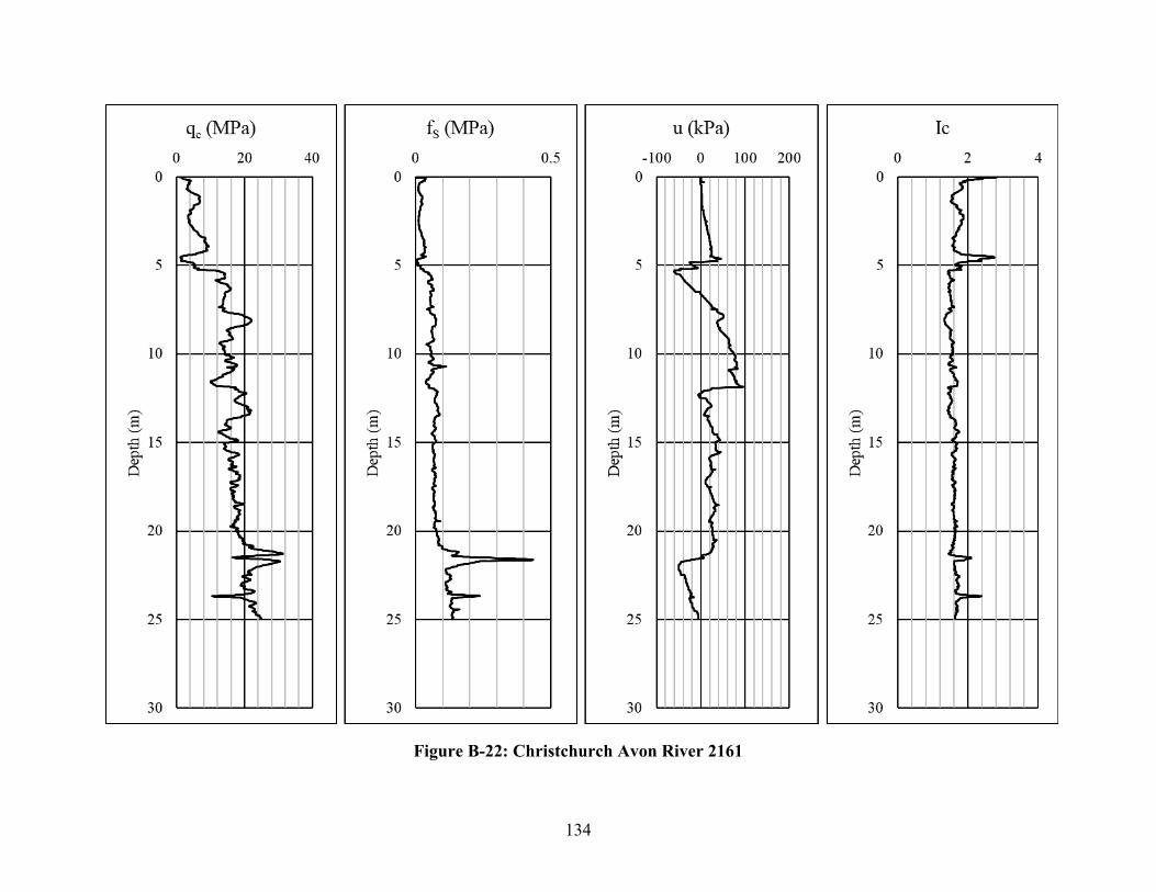
134
Figure B-22: Christchurch Avon River 2161

135
Figure B-23: Christchurch Avon River 2242

136
Figure B-24: Christchurch Avon River 2319

137
Figure B-25: Christchurch Avon River 2333

138
Figure B-26: Christchurch Avon River 26641

139
Figure B-27: Christchurch Avon River 27046

140
Figure B-28: Christchurch Avon River 29053

141
Figure B-29: Christchurch Avon River 29058

142
Figure B-30: Christchurch Avon River 325

143
Figure B-31: Christchurch Avon River 34460

144
Figure B-32: Christchurch Avon River 34616

145
Figure B-33: Christchurch Avon River 38115

146
Figure B-34: Christchurch Avon River 38121

147
Figure B-35: Christchurch Avon River 3924

148
Figure B-36: Christchurch Avon River 4643

149
Figure B-37: Christchurch Avon River 4985

150
Figure B-38: Christchurch Avon River 5252

151
Figure B-39: Christchurch Avon River 6382

152
Figure B-40: Christchurch Avon River 64

153
Figure B-41: Christchurch Avon River 71

154
Figure B-42: Christchurch Avon River 9712

155
Figure B-43: Imperial Valley Heber 1

156
Figure B-44: Imperial Valley Heber 2

157
Figure B-45: Imperial Valley Heber 3

158
Figure B-46: Imperial Valley Heber 4

159
Figure B-47: Imperial Valley Heber 442

160
Figure B-48: Imperial Valley Heber 5

161
Figure B-49: Imperial Valley Heber 6

162
Figure B-50: Imperial Valley Heber 7

163
Figure B-51: Imperial Valley Heber 700-lsu006

164
Figure B-52: Imperial Valley Heber 8

165
Figure B-53: Imperial Valley Riverpark pqs1

166
Figure B-54: Imperial Valley Riverpark pqs2

167
Figure B-55: Imperial Valley Riverpark pqs3

168
Figure B-56: Imperial Valley Riverpark pqs4

169
Figure B-57: Imperial Valley Riverpark pqs5

170
Figure B-58: Loma Prieta Moss Landing UC-18

171
Figure B-59: Loma Prieta Moss Landing UC-2

172
Figure B-60: Loma Prieta Moss Landing UC-3

173
Figure B-61: Loma Prieta Moss Landing UC-4

174
Figure B-62: Loma Prieta Moss Landing UC-5

175
Figure B-63: Loma Prieta Moss Landing UC-6

176
Figure B-64: Northridge Balboa 1

177
Figure B-65: Northridge Balboa 10

178
Figure B-66: Northridge Balboa 11

179
Figure B-67: Northridge Balboa 12

180
Figure B-68: Northridge Balboa 13

181
Figure B-69: Northridge Balboa 13.5

182
Figure B-70: Northridge Balboa 15

183
Figure B-71: Northridge Balboa 16

184
Figure B-72: Northridge Balboa 2

185
Figure B-73: Northridge Balboa 3

186
Figure B-74: Northridge Balboa 4

187
Figure B-75: Northridge Balboa 5

188
Figure B-76: Northridge Balboa 6

189
Figure B-77: Northridge Balboa 7

190
Figure B-78: Northridge Balboa 8

191
Figure B-79: Northridge Balboa 9

192
Figure B-80: Northridge Malden 11

193
Figure B-81: Northridge Malden 12
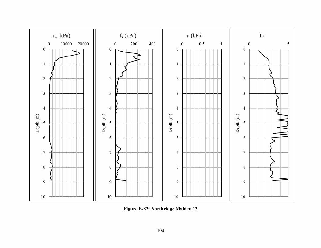
194
Figure B-82: Northridge Malden 13

195
Figure B-83: Northridge Malden 3

196
Figure B-84: Northridge Malden 4

197
Figure B-85: Northridge Malden 5

198
Figure B-86: Northridge Potrero 1

199
Figure B-87: Northridge Potrero 10

200
Figure B-88: Northridge Potrero 11

201
Figure B-89: Northridge Potrero 12

202
Figure B-90: Northridge Potrero 3

203
Figure B-91: Northridge Potrero 4

204
Figure B-92: Northridge Potrero 5

205
Figure B-93: Northridge Potrero 6
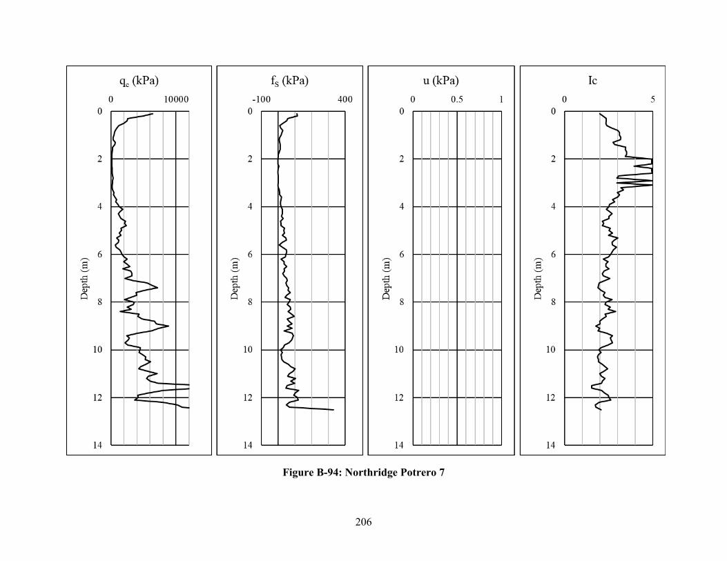
206
Figure B-94: Northridge Potrero 7

207
Figure B-95: Northridge Potrero 8

208
Figure B-96: Northridge Potrero 9

209
Figure B-97: Northridge Wynne 1

210
Figure B-98: Northridge Wynne 10

211
Figure B-99: Northridge Wynne 11

212
Figure B-100: Northridge Wynne 12

213
Figure B-101: Northridge Wynne 13

214
Figure B-102: Northridge Wynne 14

215
Figure B-103: Northridge Wynne 2

216
Figure B-104: Northridge Wynne 3

217
Figure B-105: Northridge Wynne 4

218
Figure B-106: Northridge Wynne 5

219
Figure B-107: Northridge Wynne 7

220
Figure B-108: Northridge Wynne 8

221
Figure B-109: San Fernando Juvenile Hall sfvjh81-2

222
Figure B-110: San Fernando Juvenile Hall sfvjh81-4

223
Figure B-111: San Fernando Juvenile Hall sfvjh81-6

224
Figure B-112: San Fernando Juvenile Hall sfvjh9

225
Figure B-113: Taiwan MAA C9

226
Figure B-114: Taiwan NCC 2

227
Figure B-115: Taiwan NCC 3
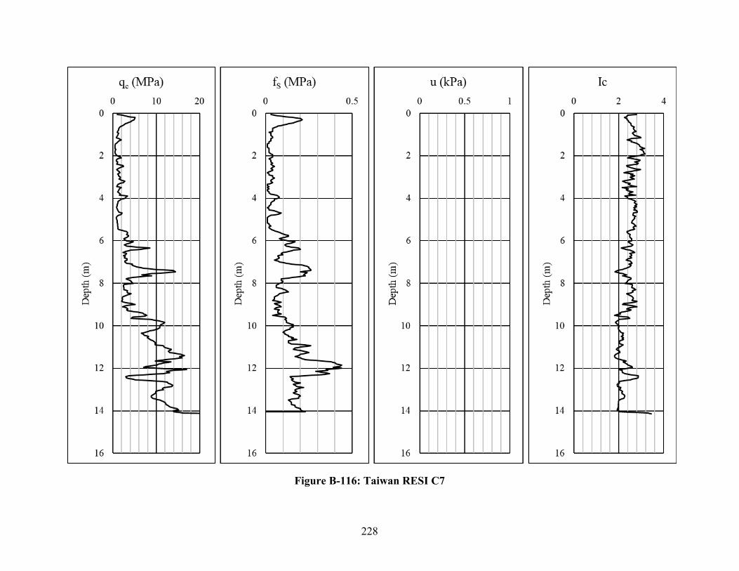
228
Figure B-116: Taiwan RESI C7

229
Figure B-117: Taiwan WBC 1

230
Figure B-118: Taiwan WBC 4

231
Figure B-119: Taiwan WCC 1

232
Figure B-120: Taiwan WCC 11

233
Figure B-121: Taiwan WCC 12

234
Figure B-122: Taiwan WCC 13

235
Figure B-123: Taiwan WCC 2

236
Figure B-124: Taiwan WCC 4

237
Figure B-125: Taiwan WCC 6

238
Figure B-126: Taiwan WCC 7

239
Figure B-127: Taiwan WCC 8

240
Figure B-128: Taiwan WCC 9

241
Figure B-129: Turkey Cark 24
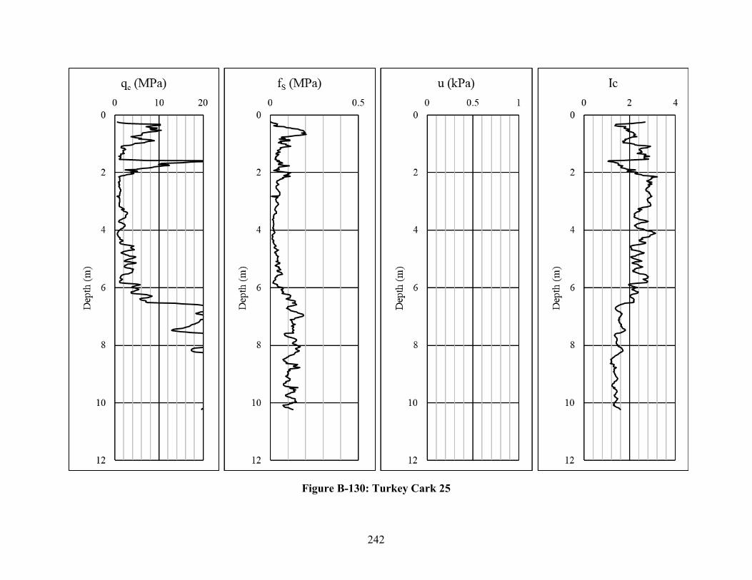
242
Figure B-130: Turkey Cark 25

243
Figure B-131: Turkey Cumhuriyet 22

244
Figure B-132: Turkey Cumhuriyet 23

245
Figure B-133: Turkey Cumhuriyet 24

246
Figure B-134: Turkey Degirmendere dn1

247
Figure B-135: Turkey Degirmendere dn2

248
Figure B-136: Turkey Degirmendere dn3