analysis article discovery · the model space is discretized using staggered arakawa c grid. we...

© 2015 Discovery Publication. All Rights Reserved. www.discoveryjournals.com OPEN ACCESS

ARTICLE

Page

173

ANALYSIS

High resolution simulation of the salinity variability in the Bay of Bengal and Arabian Sea during the years 1998-2014 using an ocean circulation model Alok Kumar Mishra1☼, Suneet Dwivedi2, Atul Shrivastava3 1. K.Banerjee Centre of Atmospheric and Ocean Studies, University of Allahabad, Allahabad, India; Email:[email protected] 2. K.Banerjee Centre of Atmospheric and Ocean Studies, University of Allahabad, Allahabad, India; Email:[email protected] 3. K.Banerjee Centre of Atmospheric and Ocean Studies, University of Allahabad, Allahabad, India; Email:[email protected] ☼Corresponding author: K.Banerjee Centre of Atmospheric and Ocean Studies, University of Allahabad, Allahabad, India; Email:[email protected] Publication History Received: 17 June 2015 Accepted: 04 August 2015 Published: 1 September 2015 Citation Alok Kumar Mishra, Suneet Dwivedi, Atul Shrivastava. High resolution simulation of the salinity variability in the Bay of Bengal and Arabian Sea during the years 1998-2014 using an ocean circulation model. Discovery, 2015, 39(180), 173-179 Publication License

This work is licensed under a Creative Commons Attribution 4.0 International License. General Note

Article is recommended to print as color digital version in recycled paper.

ABSTRACT A high resolution ocean general circulation model with a horizontal resolution of 10 Km is used to investigate salinity in the Northern Indian Ocean [65E-95E; 5N-20N]. The model simulated salinity during the years 1998-2014 is compared against the satellite and in-situ observations. The model is able to capture the contrasting distributions of sea surface salinity (SSS) in the Arabian Sea and the Bay of Bengal. The Bay of Bengal salinity values are generally lower than the Arabian Sea. The model is also able to reproduce the strong seasonality of the sea surface salinity in the changing climate. The inter-annual SSS variability is 2-4 times

ANALYSIS 39(180), September 1, 2015

Discovery ISSN 2278–5469

EISSN 2278–5450


ARTICLE

Page

174

ANALYSIS

smaller than seasonal variability in the region of study. The regions of large inter-annual variability are located near river mouths in the Bay of Bengal. The inter-annual variability of the SSS in the northern Indian ocean is also examined in the light of recent changes in the El Nino-Southern Oscillation (ENSO), Indian Ocean Dipole (IOD) during the period of study. The relative role of wind and solar radiation on the sea surface salinity is also investigated. Keywords: Ocean Circulation Modeling, Sea Surface Salinity, Northern Indian Ocean. 1. INTRODUCTION The northern Indian Ocean is forced by semi-annually reversing winds that blow from the south west during the summer monsoon and from the north-east during the winter monsoon. The Strong evaporation over precipitation and inflow from the Red Sea and Persian Gulf makes the Arabian Sea (AS) much saltier (Antonov et al., 2010; Chatterjee et al., 2012). In contrast to this, the Bay of Bengal (BoB) experiences high precipitation and river discharge by adjoining river Ganga, Brahmaputra and Irrawaddy during the monsoon and post-monsoon months (Rao et al., 2003; Sengupta et al., 2006; Durand et al., 2011). The river runoff is entering initially through mouth of river and advected into the southern BoB and then in the eastern AS by the East India Coastal Current (Vinayachandran et al., 2007). The yearly freshwater flux (precipitation plus river runoff) received by the BoB is largely exceeds the freshwater flux evaporated back to the atmosphere (Shenoi et al., 2002; Sengupta et al., 2006). As a result, sea surface salinity (SSS) of northern BoB is very low (Parampil et al., 2010; Han et al., 2001) and highly stratified. These fresh near surface waters affects the depth of wind-induced vertical mixing which is responsible for shallow mixed layers in the northern BoB (Lukas and Lindstorm 1991, de Boyer Montegut et al., 2007, Girishkumar et al., 2013). Due to high stratification in northern BoB, formation of barrier layer takes place which prevents the entrainment of cool, deep water in to surface which is responsible for making warmer upper ocean temperature of BoB. The salinity stratification helps in reducing the cooling effects during cyclone in the BoB, which prone to intensification of tropical cyclones (Sengupta et al., 2008; Neetu et al., 2012). This low SSS and stratification in the BoB is also influence the regional climate. It also affects the climate of the Indian subcontinent including the summer monsoon rainfall thus affecting lives of billions of people living there. Salinity also modulates the intra-seasonal variability of the SST in the Northern Bay of Bengal (Vinayachandran et al., 2012).The SSS observation in Northern Indian Ocean is very sparse in space as well as in time. For better description of the SSS seasonal evolution within the Northern Indian Ocean, and to assess all the processes that govern the seasonal SSS evolution, the observation data are not yet quantitatively sufficient. So Numerical ocean circulation models have the distinct advantage of generating long time series of salinity at high spatial and temporal resolution which can help in understanding processes responsible for salinity variability. The role of river runoff, precipitation, and advection of fresh water from northern BoB to AS through EICC have been identified through sensitivity experiment using modelling study (Diansky et al., 2006; Wu et al., 2007; Sharma et al., 2010; Girishkumar et al., 2013; Benshila et al., 2013; Akhil et al., 2014; Chaitanya et al., 2015). The seasonality of sea surface variability is strongly influence by monsoonal current (Shankar et al., 2002) which advect low salinity water of BoB into AS during Winter monsoon season and high salinity water of AS into BoB during summer monsoon season. The salinity is important parameter for understanding the ocean hydrological cycle, which is least understood and important component of the climate system (Schmitt, 1994), it plays an important role in controlling near-surface vertical mixing and affect several climatic phenomena, i.e. Tropical cyclone, monsoon rainfall (Sanilkumar et al., 1994; Vinayachandran et al., 2015).

In this paper, we describe the surface and subsurface salinity variability on seasonal and interannual time scales using a high resolution ocean model and estimate the contribution of wind and solar radiation in modulation of the salinity. In section 2, we describe the configuration of the ocean model used for the study and details on setup of sensitivity experiments. In section 3, we describe the validation of model results. In section 4, we describe the surface and subsurface salinity variability on the seasonal and interannual time scales. We describe the contribution of wind and solar radiation on salinity using the sensitivity experiments in Section 5. Conclusions are in Section 6.

2. MODEL CONFIGURATION We use the MIT General Circulation Model (MITgcm) (Marshall et al., 1997) to carry out the present study. The MITgcm is a z-coordinate model, which uses hydrostatic approximation. The model space is discretized using staggered Arakawa C grid. We configure the model at a high horizontal resolution of 10 km in the Bay of Bengal region around [65E-95E; 5N-20N] during 1 Jan 1998 to 31 Dec 2014. The highest vertical resolution is taken as 5 m near the ocean surface and then gradually telescoping out at depth. We used a total of 28 vertical levels with maximum vertical spacing of 500 m near the ocean floor. The model uses open boundary conditions on all four sides, which are taken from the ORAS4. We used the KPP non-local vertical mixing scheme (Large et


ARTICLE

Page

175

ANALYSIS

al., 1994) to resolve the sub-grid scale processes. The eddy (harmonic) viscosity and diffusivity satisfying the CFL stability criterion is chosen in horizontal and vertical. We use no-slip condition on sides as well as bottom. The bottom frictional drag coefficient is taken as 0.001. A 3rd order direct space-time advection scheme is employed for temperature and salinity. The bathymetry of the region of interest in the BoB (Figure 1) is taken from the Smith and Sandell (1997) 1’ bathymetry data. The nonlinear equation of state is used following the Jackett and McDougall (1995). The initial temperature and salinity are derived from the World Ocean Atlas 2013 (WOA13) data (Locarnini et al., 2013; Zweng et al., 2013). The 6-hourly NCEP/NCAR reanalysis (Kalnay et al., 1996) forcing, namely, 2m air temperature, humidity, downward long-wave and short-wave radiations, precipitation, zonal and meridional winds and runoff are used to force the model. Evaporation are calculated by model itself using bulk formula. Model is relaxed with monthly climatology of SST and SSS from WOA13.

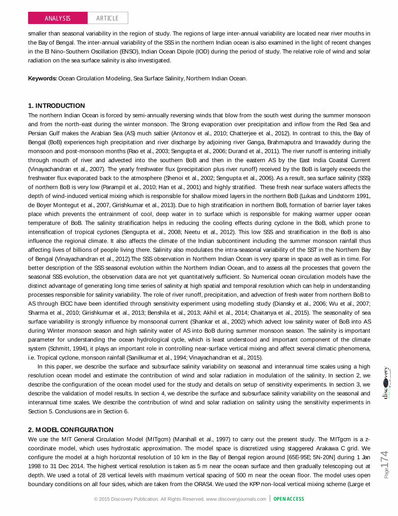
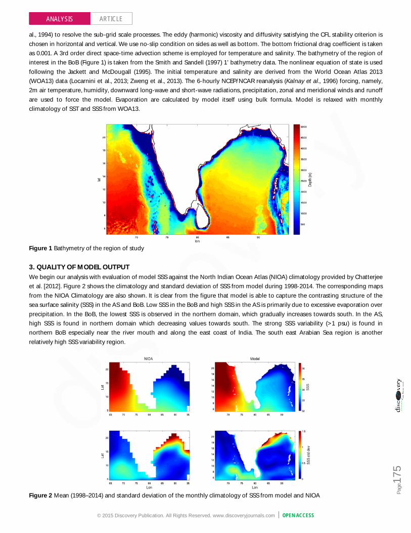
Figure 1 Bathymetry of the region of study 3. QUALITY OF MODEL OUTPUT We begin our analysis with evaluation of model SSS against the North Indian Ocean Atlas (NIOA) climatology provided by Chatterjee et al. [2012]. Figure 2 shows the climatology and standard deviation of SSS from model during 1998-2014. The corresponding maps from the NIOA Climatology are also shown. It is clear from the figure that model is able to capture the contrasting structure of the sea surface salinity (SSS) in the AS and BoB. Low SSS in the BoB and high SSS in the AS is primarily due to excessive evaporation over precipitation. In the BoB, the lowest SSS is observed in the northern domain, which gradually increases towards south. In the AS, high SSS is found in northern domain which decreasing values towards south. The strong SSS variability (>1 psu) is found in northern BoB especially near the river mouth and along the east coast of India. The south east Arabian Sea region is another relatively high SSS variability region.

Figure 2 Mean (1998–2014) and standard deviation of the monthly climatology of SSS from model and NIOA


ARTICLE

Page

176

ANALYSIS

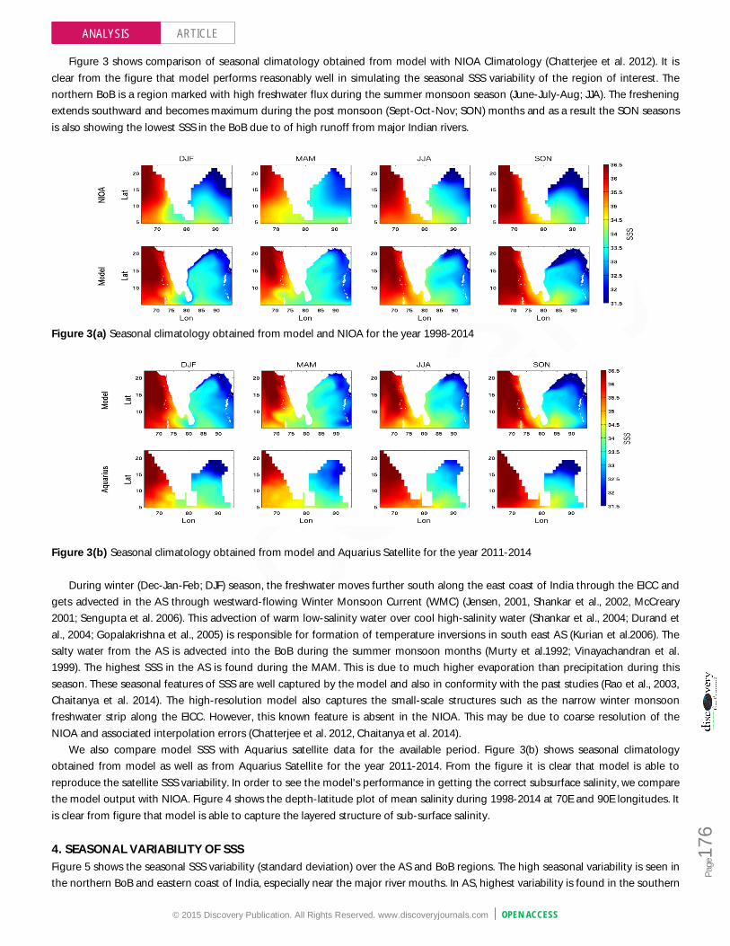
Figure 3 shows comparison of seasonal climatology obtained from model with NIOA Climatology (Chatterjee et al. 2012). It is clear from the figure that model performs reasonably well in simulating the seasonal SSS variability of the region of interest. The northern BoB is a region marked with high freshwater flux during the summer monsoon season (June-July-Aug; JJA). The freshening extends southward and becomes maximum during the post monsoon (Sept-Oct-Nov; SON) months and as a result the SON seasons is also showing the lowest SSS in the BoB due to of high runoff from major Indian rivers.

Figure 3(a) Seasonal climatology obtained from model and NIOA for the year 1998-2014

Figure 3(b) Seasonal climatology obtained from model and Aquarius Satellite for the year 2011-2014

During winter (Dec-Jan-Feb; DJF) season, the freshwater moves further south along the east coast of India through the EICC and gets advected in the AS through westward-flowing Winter Monsoon Current (WMC) (Jensen, 2001, Shankar et al., 2002, McCreary 2001; Sengupta et al. 2006). This advection of warm low-salinity water over cool high-salinity water (Shankar et al., 2004; Durand et al., 2004; Gopalakrishna et al., 2005) is responsible for formation of temperature inversions in south east AS (Kurian et al.2006). The salty water from the AS is advected into the BoB during the summer monsoon months (Murty et al.1992; Vinayachandran et al. 1999). The highest SSS in the AS is found during the MAM. This is due to much higher evaporation than precipitation during this season. These seasonal features of SSS are well captured by the model and also in conformity with the past studies (Rao et al., 2003, Chaitanya et al. 2014). The high-resolution model also captures the small-scale structures such as the narrow winter monsoon freshwater strip along the EICC. However, this known feature is absent in the NIOA. This may be due to coarse resolution of the NIOA and associated interpolation errors (Chatterjee et al. 2012, Chaitanya et al. 2014).

We also compare model SSS with Aquarius satellite data for the available period. Figure 3(b) shows seasonal climatology obtained from model as well as from Aquarius Satellite for the year 2011-2014. From the figure it is clear that model is able to reproduce the satellite SSS variability. In order to see the model's performance in getting the correct subsurface salinity, we compare the model output with NIOA. Figure 4 shows the depth-latitude plot of mean salinity during 1998-2014 at 70E and 90E longitudes. It is clear from figure that model is able to capture the layered structure of sub-surface salinity. 4. SEASONAL VARIABILITY OF SSS Figure 5 shows the seasonal SSS variability (standard deviation) over the AS and BoB regions. The high seasonal variability is seen in the northern BoB and eastern coast of India, especially near the major river mouths. In AS, highest variability is found in the southern


ARTICLE

Page

177

ANALYSIS

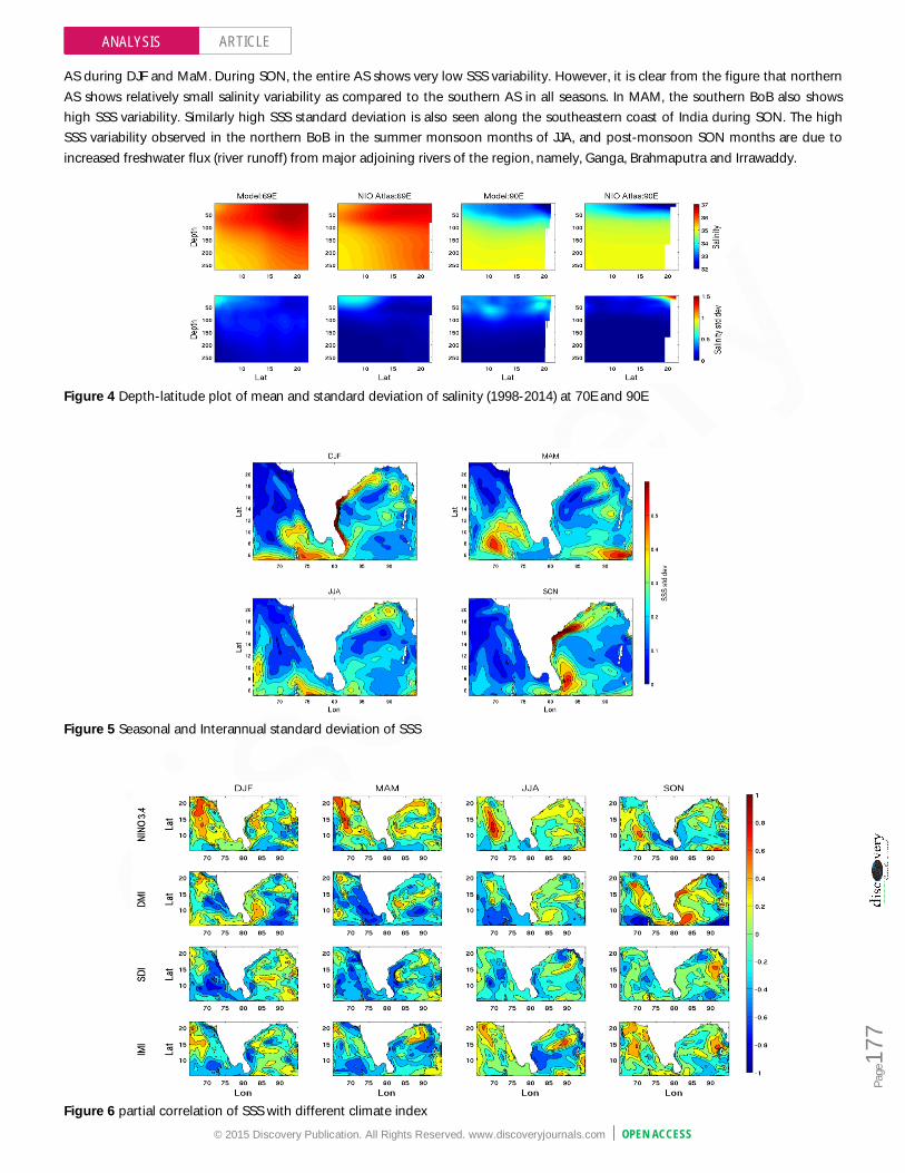
AS during DJF and MaM. During SON, the entire AS shows very low SSS variability. However, it is clear from the figure that northern AS shows relatively small salinity variability as compared to the southern AS in all seasons. In MAM, the southern BoB also shows high SSS variability. Similarly high SSS standard deviation is also seen along the southeastern coast of India during SON. The high SSS variability observed in the northern BoB in the summer monsoon months of JJA, and post-monsoon SON months are due to increased freshwater flux (river runoff) from major adjoining rivers of the region, namely, Ganga, Brahmaputra and Irrawaddy.

Figure 4 Depth-latitude plot of mean and standard deviation of salinity (1998-2014) at 70E and 90E

Figure 5 Seasonal and Interannual standard deviation of SSS

Figure 6 partial correlation of SSS with different climate index


ARTICLE

Page

178

ANALYSIS

5. RELATION OF SSS WITH DIFFERENT CLIMATE MODES In order to examine variability of the SSS patterns over the AS and BoB vis-à-vis variability of the known climate indices, we find the spatial correlation (Figure 6) of SSS with the time series of NINO3.4, Dipole Mode Index (DMI), Southern Dipole Index (SDI) and Indian Monsoon Index (IMI).

From figure 6, it is clear that SSS variability over the AS and BoB is influenced by the ENSO, IOD, SIOD and monsoon variability. The correlation of NINO3.4 is highest in the AS in all seasons. DMI has highest correlation in autumn in eastern coast of India and eastern Arabian Sea with correlation ranging from 0.6 to 0.75. On the other hand, the south eastern BoB and south western AS show negative DMI correlation in the range of -0.6 to -0.9. 6. CONCLUSION The goal of present study is threefold: (i) to demonstrate the quality of salinity derived from the high resolution general circulation model in the Arabian Sea and Bay of Bengal; (ii) to explore the variability of surface and subsurface salinity; (iii) to assess the role of near surface wind and solar radiation on the seasonal variability of SSS. The SSS from model is found to be in good agreement with the satellite and in-situ observations. The model is able to reproduce the distinct SSS features in the AS and BoB. The model also captures small-scale structures such as the narrow winter monsoon freshwater strip along the EICC. This feature is seen only in the high-resolution model output, whereas, it is absent in the coarse resolution reanalysis data. The inter-annual SSS variability is 2-4 times smaller than seasonal variability in entire study domain. The regions of large SSS variability are located near the river mouths in the Bay of Bengal. The SSS also gets influenced by different climate modes. The spatial correlation of SSS with NINO3.4 is higher in AS than BoB for all seasons. The DMI has highest correlation in autumn along the eastern coast of India and eastern Arabian Sea. On the other hand, south eastern BoB and south western AS show negative correlation with SSS. The SSS is also strongly affected by the wind and solar radiation. The SSS decreases in the absence of wind as well as solar radiation. ACKNOWLEDGMENTS AKM and AS are thankful to the MoES/ISRO for providing Junior Research Fellowship. SD is thankful to the NCAOR/ISRO/DST for financial assistance in the form of research project. Thanks are also to the WOA, NCEP/NCAR, TMI, NIOA and ORAS4 for making their data freely available for research purpose. REFERENCE 1. Akter, N.and K. Tsuboki, K. (2014). Role of synoptic-scale

forcing in cyclogenesis over the Bay of Bengal. Climate Dynamics 43: 2651-2662, 10.1007/s00382-014-2077-9.

2. Babu, M. T., Sarma, Y. V. B., Murty, V. S. N. and Vethamony, P. (2003). On the circulation in the Bay of Bengal during northern spring intermonsoon (March-April 1987), Deep Sea Res., Part II, 50(5), 855–865.

3. Benshila, R., Durand, F., Masson, S., Bourdalle-Badie, R., de Boyer Montégut, C. and PapaF,Madec G. (2014). The upper Bay of Bengal salinity structure in a high-resolution model. Ocean Modelling 74:36-52.

4. Chaitanya, A. V. S., Durand, F., Mathew, S., Gopalakrishna, V.V., Papa, F., Lengaigne, M. and Venkatesan,R. (2015). Observed year-to-year sea surface salinity variability in the Bay of Bengal during the 2009–2014 period. Ocean Dynamics 65: 173-186.

5. Chatterjee, A., Shankar, D., Shenoi, S. S. C., Reddy, G. V., Michael, G. S., Ravichandran, M., Gopalkrishna, V. V., Rao, E. P. R., Bhaskar, T. V. S. U., Sanjeevan, V. N. (2012). A new atlas of temperature and salinity for the North Indian Ocean. J. Earth Sys. Sci. 121, 559-593.

6. Jackett, D. R. and McDougall, T. J. (1995). Minimal adjustment of hydrographic profiles to achieve static

stability. J. Atmos. Ocean. Technol. 12: 381-389. 7. Kalnay, E., et al. 1996. The NCEP/NCAR 40-year reanalysis

project. Bull. Amer. Meteor. Soc. 77, 437-470. 8. Large, W. G., McWilliams, J. C. and Doney, S. C. (1994).

Oceanic vertical mixing: A review and a model with a nonlocal boundary layer parameterization. Rev. Geophys. 32, 363-403.

9. Locarnini, R. A., Mishonov, A. V., Antonov, J. I., Boyer, T. P., Garcia, H. E., Baranova, O. K., Zweng, M. M., Paver, C. R., Reagan, J. R., Johnson, D. R., Hamilton, M. and Seidov, D. (2013). World Ocean Atlas 2013, Vol. 1. Temperature. S. Levitus, Ed., A. Mishonov Technical Ed.; NOAA Atlas NESDIS 73, 40 pp.

10. Marshall, J., Adcroft, A., Hill,C., Perelman, L. and Heisey, C. (1997). A finite-volume, incompressible Navier-Stokes model for studies of the ocean on parallel computers. J. Geophys. Res.102: 5753-5766.

11. Masson, S. and Coauthors. (2005): Impact of barrier layer on winter-spring warming of the South-Eastern Arabian Sea. Geophys. Res. Lett., 32, L07703, doi: 10.1029/2004GL021980.

12. McCreary, J., Kundu, P. and Molinari, R. (1993). A numerical investigation of dynamics, thermodynamics and mixed-layer processes in the Indian Ocean, Progr. Oceanogr. 31(3), 181–


ARTICLE

Page

179

ANALYSIS

244. 13. Neetu, S., Lengaigne, M., Vincent, E.M., Vialard, J., Madec, G.,

Samson, G., Ramesh Kumar, M.R., Durand, F. (2012).Influence of upper-ocean stratification on tropical cyclone-induced surface cooling in the Bay of Bengal. J Geophys Res 117(C12020).doi:10.1029/2012JC008433.

14. Vinayachandran, P. N., Jahfer, S. And Nanjundiah, R.S. (2015). Impact of river runoff into the ocean on Indian summer monsoon, Environ. Res. Lett. 10, doi:10.1088/1748-9326/10/5/054008.

15. Schmitt, R. W. (1994).The ocean freshwater cycle, report of JSC Ocean Observing System Development Panel, Tex. A and M Univ., College Station.

16. Sengupta, D., Bharath, R. G. and Shenoi, S. S. C. (2006).Surface freshwater from Bay of Bengal runoff and Indonesian through flow in the tropica l Indian Ocean. Geophys. Res. Lett. 33 L22609.

17. Sharma, R., Agarwal, N., Momin, I. M., Basu, S. and Agarwal, V. K. (2010). Simulated sea surface salinity variability in the tropical Indian Ocean, J. Clim. 23, 6542–6554.

18. Smith, W. H. F. and Sandwell, D. T. (1997). Global seafloor topography from satellite altimetry and ship depth soundings. Science. 277, 1957-1962.

19. Vinayachandran, P. N., Neema, C. P., Mathew, S. and R. Remya.R. (2012). Mechanisms of summer intraseasonal sea surface temperature oscillations in the Bay of Bengal. J. Geophys. Res. 117, C01005, doi: 10.1029/2011JC007433.

20. Vinayachandran, P. N., Shankar, D., Vernekar, S., Sandeep, K. K., Amol, P., Neema, C. P. and Chatterjee, A. (2013). A summer monsoon pump to keep the Bay of Bengal salty, Geophys. Res. Lett., 40, 1777–1782, doi:10.1002/grl.50274.

21. Vinayachandran, PN., S Jahfer and RS Nanjundiah (2015): Impact of river runoff into the ocean on Indian summer monsoon, Environ. Res. Lett. 10, doi:10.1088/1748-9326/10/5/054008.

analysis article discovery · the model space is discretized using staggered arakawa c grid. we...

Documents