analysis and optimization of four-coil planar magnetically ... · the primary and secondary coils...

sensors

Article

Analysis and Optimization of Four-Coil PlanarMagnetically Coupled Printed Spiral Resonators

Sadeque Reza Khan and GoangSeog Choi *

Department of Information and Communication Engineering, SoC Design Laboratory, Chosun University,Gwangju 61452, Korea; [email protected]* Correspondence: [email protected]; Tel.: +82-62-230-7716

Academic Editor: Vittorio M. N. PassaroReceived: 2 June 2016; Accepted: 29 July 2016; Published: 3 August 2016

Abstract: High-efficiency power transfer at a long distance can be efficiently established usingresonance-based wireless techniques. In contrast to the conventional two-coil-based inductive links,this paper presents a magnetically coupled fully planar four-coil printed spiral resonator-basedwireless power-transfer system that compensates the adverse effect of low coupling and improvesefficiency by using high quality-factor coils. A conformal architecture is adopted to reduce thetransmitter and receiver sizes. Both square architecture and circular architectures are analyzedand optimized to provide maximum efficiency at a certain operating distance. Furthermore, theirperformance is compared on the basis of the power-transfer efficiency and power delivered to theload. Square resonators can produce higher measured power-transfer efficiency (79.8%) than circularresonators (78.43%) when the distance between the transmitter and receiver coils is 10 mm of airmedium at a resonant frequency of 13.56 MHz. On the other hand, circular coils can deliver higherpower (443.5 mW) to the load than the square coils (396 mW) under the same medium properties.The performance of the proposed structures is investigated by simulation using a three-layerhuman-tissue medium and by experimentation.

Keywords: bio-implantable devices; magnetic resonance coupling; power delivered to the load;power-transfer efficiency; quality factor

1. Introduction

Wireless power-transmission systems based on inductive coupling are extensively used inimplantable microelectronic devices to increase patient’s comfort and reduce the risk of infectiondue to the use of transcutaneous wires or the chemical side effects of a battery. The size and lifetime ofthe battery is another issue of concern in powering bio-implantable devices. The smallest possible sizeis a major requirement for bio-implants. Depending on its size, the functional depth of an implantabledevice in a human biological tissue is determined. Usually, these devices are placed in less than10 mm of depth in human tissue. General implanted microsystems are placed at 1–4 mm of depth.Cochlear implants need to be placed at 3–6 mm inside the temporal bone, and for retinal implants, theexpected depth is 5 mm [1–3].

The applications of wireless power transmission span over a broad range from submicrowatt tofew kilowatts [4–12]. Inductive-coupling-based wireless power transfer (WPT) systems are commonlyused for implantable devices [13–18]. The primary and secondary coils are used as the transmitter(TX) and receiver (RX), respectively, in a two-coil-based inductively coupled WPT. A two-coil-basedWPT system suffers from low quality factor (Q-factor or Q) and low coupling coefficient (k) due tothe source and load resistances. Hence, the maximum achievable power-transfer efficiency (PTE)is relatively low in such systems [19–21]. Moreover, most of the previous coils are designed basedon filament or Litz wire. The manufacturing and reduction of the size of such coils require proper

Sensors 2016, 16, 1219; doi:10.3390/s16081219 www.mdpi.com/journal/sensors

http://www.mdpi.com/journal/sensors

http://www.mdpi.com

http://www.mdpi.com/journal/sensors

Sensors 2016, 16, 1219 2 of 24

expertise and sophisticated machinery. As a result, planar and lithographically defined printed spiralcoils (PSCs) were introduced in [22]. Flexibility and geometric compactness make the PSC suitable forbiomedical devices.

The PTE of a WPT system depends on the architecture (dimension and structure) of the coils,physical spacing between the coils, relative location, and environment of the coils. The mutual spacingbetween the TX (or external coil) and RX (or implanted coil) of a biomedical implant must be smallerthan the wavelength in the near field and it depends on the dimensions of the coils. The implanted coilmust be carefully designed as it is located inside the human body, and it should be as small as possible.

An efficient power-transfer method is required for bio-implants to satisfy the power specificationand safety issues. Thus, resonant-based power delivery technique has become popular nowadays.This WPT technique typically uses four coils (source, primary, secondary, and load) [23]. The sourceand primary coils as well as the secondary and load coils are coupled by inductive link. In the TXside, a pair of coils, which are referred to as the source (coil 1 or C1) and primary (coil 2 or C2) coils isused, shown in Figure 1. Another pair of coils, which are referred to as the secondary (coil 3 or C3) andload (coil 4 or C4) coils is used on the RX side. All the coils are tuned at the same resonance frequency(fres) by C1–C4 capacitors. R1–R4 are parasitic resistances. Li, where i = 1 to 4, is the self-inductance ofthe coil. Mij and kc.ij represent the mutual inductance and coupling coefficient, respectively, of twoadjacent coils. In four-coil-based WPT, the TX coil stores energy in the same way as a discrete LC tank.TX coil can be modeled as a tuned step-up transformer as well, where the source can be representedas a primary of the transformer and it can be connected to the source through a power amplifier.The primary of the TX coil can be modeled as the secondary of the transformer which is left open.The RX functions in a similar manner as a step-down transformer. In contrast with the two-coil-basedWPT, the effect of source and load resistance can be reduced by the C1 and C4, respectively, in afour-coil WPT, thus can enhance the overall PTE. In a four-coil-based WPT, a high matching conditioncan be achieved by adjusting the coupling coefficient between source-primary and secondary-loadcoils. Therefore, it is possible to transfer high power to the load. The distance between TX and RXis 10–20 mm, and the separation medium is human biological tissue. The architecture of the TX andRX coils shown in Figure 1 is conformal [24–26] or fully planar [27]. This structure eliminates thepossibility of misalignment between coil 1 and coil 2 as well as between coil 3 and coil 4 [28]. Thus, thismethod improves the overall PTE under misalignment conditions.

Sensors 2016, 16, 1219 2 of 24

expertise and sophisticated machinery. As a result, planar and lithographically defined printed spiral coils (PSCs) were introduced in [22]. Flexibility and geometric compactness make the PSC suitable for biomedical devices.

The PTE of a WPT system depends on the architecture (dimension and structure) of the coils, physical spacing between the coils, relative location, and environment of the coils. The mutual spacing between the TX (or external coil) and RX (or implanted coil) of a biomedical implant must be smaller than the wavelength in the near field and it depends on the dimensions of the coils. The implanted coil must be carefully designed as it is located inside the human body, and it should be as small as possible.

An efficient power-transfer method is required for bio-implants to satisfy the power specification and safety issues. Thus, resonant-based power delivery technique has become popular nowadays. This WPT technique typically uses four coils (source, primary, secondary, and load) [23]. The source and primary coils as well as the secondary and load coils are coupled by inductive link. In the TX side, a pair of coils, which are referred to as the source (coil 1 or C1) and primary (coil 2 or C2) coils is used, shown in Figure 1. Another pair of coils, which are referred to as the secondary (coil 3 or C3) and load (coil 4 or C4) coils is used on the RX side. All the coils are tuned at the same resonance frequency (fres) by C1–C4 capacitors. R1–R4 are parasitic resistances. Li, where i = 1 to 4, is the self-inductance of the coil. Mij and kc.ij represent the mutual inductance and coupling coefficient, respectively, of two adjacent coils. In four-coil-based WPT, the TX coil stores energy in the same way as a discrete LC tank. TX coil can be modeled as a tuned step-up transformer as well, where the source can be represented as a primary of the transformer and it can be connected to the source through a power amplifier. The primary of the TX coil can be modeled as the secondary of the transformer which is left open. The RX functions in a similar manner as a step-down transformer. In contrast with the two-coil-based WPT, the effect of source and load resistance can be reduced by the C1 and C4, respectively, in a four-coil WPT, thus can enhance the overall PTE. In a four-coil-based WPT, a high matching condition can be achieved by adjusting the coupling coefficient between source-primary and secondary-load coils. Therefore, it is possible to transfer high power to the load. The distance between TX and RX is 10–20 mm, and the separation medium is human biological tissue. The architecture of the TX and RX coils shown in Figure 1 is conformal [24–26] or fully planar [27]. This structure eliminates the possibility of misalignment between coil 1 and coil 2 as well as between coil 3 and coil 4 [28]. Thus, this method improves the overall PTE under misalignment conditions.

Figure 1. Simplified physical and electrical configuration of a fully planar WPT in a human tissue medium.

In this paper, a fully planar four-coil magnetic resonance coupling (MRC)-based WPT is analyzed using circuit-based modeling. Both square and circular architectures are considered for analysis and optimization for asymmetrical spiral inductors. The reflected-load theory [29] is used to

Figure 1. Simplified physical and electrical configuration of a fully planar WPT in a humantissue medium.

In this paper, a fully planar four-coil magnetic resonance coupling (MRC)-based WPT is analyzedusing circuit-based modeling. Both square and circular architectures are considered for analysisand optimization for asymmetrical spiral inductors. The reflected-load theory [29] is used to

Sensors 2016, 16, 1219 3 of 24

analyze the Q-factor and power delivered to the load (PDL). The accuracy of the design model isimproved by considering the effects of parasitic components as well as the surrounding environments.Critical design parameters, including the TX and RX dimensions, number of turns of the PSC,self- and mutual inductances, coupling coefficients, and Q-factors, are analytically investigated, and theoptimum design is determined by applying the design constraints through a step-by-step procedure inMATLAB. A simulation-based comparative study is done on the PTE of the MRC-WPT of both squareand circular resonators in air and the human-tissue media. Effect of misalignment on over-all PTE ischaracterized and measured as well.

This paper is organized as follows: Section 2 formulates the theoretical modeling of the MRC-WPTsystem. Section 3 describes the optimization method of the PSCs using an iterative approach byutilizing the theoretical model of Section 2 in MATLAB. Section 4 presents the simulation results,experimental setup, and necessary comparisons of the results.

2. Theoretical Modeling of MRC-WPT System

This section illustrates the individual models for the self- and mutual inductance, parasiticcomponents, and Q-factor. The models are based on both square and circular coils in the PSCarchitecture. A detailed analysis of the PTE and PDL is presented on the basis of the accurate equivalentcircuit model of the proposed MRC-WPT system. Figure 2 shows the proposed planar MRC-WPTarchitecture and the geometrical parameters of both the square- and circular-shaped coils. In Figure 2,coil 1 or coil 4 represents the source or load coil, respectively, and coil 2 or coil 3 represent the primaryor secondary coil, respectively. Din.Cx/y and Dout.Cx/y denote the inner and outer diameters, respectively.In addition, another two important parameters w.Cx/y and s.Cx/y represent the line width and spacing,respectively. The subscript “Cx/y” corresponds to a particular coil from C1 to C4.

Sensors 2016, 16, 1219 3 of 24

analyze the Q-factor and power delivered to the load (PDL). The accuracy of the design model is improved by considering the effects of parasitic components as well as the surrounding environments. Critical design parameters, including the TX and RX dimensions, number of turns of the PSC, self- and mutual inductances, coupling coefficients, and Q-factors, are analytically investigated, and the optimum design is determined by applying the design constraints through a step-by-step procedure in MATLAB. A simulation-based comparative study is done on the PTE of the MRC-WPT of both square and circular resonators in air and the human-tissue media. Effect of misalignment on over-all PTE is characterized and measured as well.

This paper is organized as follows: Section 2 formulates the theoretical modeling of the MRC-WPT system. Section 3 describes the optimization method of the PSCs using an iterative approach by utilizing the theoretical model of Section 2 in MATLAB. Section 4 presents the simulation results, experimental setup, and necessary comparisons of the results.

2. Theoretical Modeling of MRC-WPT System

This section illustrates the individual models for the self- and mutual inductance, parasitic components, and Q-factor. The models are based on both square and circular coils in the PSC architecture. A detailed analysis of the PTE and PDL is presented on the basis of the accurate equivalent circuit model of the proposed MRC-WPT system. Figure 2 shows the proposed planar MRC-WPT architecture and the geometrical parameters of both the square- and circular-shaped coils. In Figure 2, coil 1 or coil 4 represents the source or load coil, respectively, and coil 2 or coil 3 represent the primary or secondary coil, respectively. Din.Cx/y and Dout.Cx/y denote the inner and outer diameters, respectively. In addition, another two important parameters w.Cx/y and s.Cx/y represent the line width and spacing, respectively. The subscript “Cx/y” corresponds to a particular coil from C1 to C4.

Figure 2. Geometrical architecture of the square- and circular-shaped resonators.

2.1. Inductance Modeling

Self-inductance L is a function of the magnetic flux of the current-carrying conductor and the amount of current flowing through the conductor. The sides of the spirals are approximated to be symmetrical current sheets to measure the self-inductance. Adjacent sheets are considered as orthogonal with zero mutual inductance. On the other hand, the current-carrying opposite sheets have mutual inductance M. Equation (1) expresses the simplified self-inductance, which is estimated using the concept of geometric mean, arithmetic mean, and arithmetic mean square distances [30]:

2 .C .C1 0 .C

223 4

2ln

2

out x in xl x

ll l

D DC nCL C C

(1)

Figure 2. Geometrical architecture of the square- and circular-shaped resonators.

2.1. Inductance Modeling

Self-inductance L is a function of the magnetic flux of the current-carrying conductor and theamount of current flowing through the conductor. The sides of the spirals are approximated tobe symmetrical current sheets to measure the self-inductance. Adjacent sheets are considered asorthogonal with zero mutual inductance. On the other hand, the current-carrying opposite sheets havemutual inductance M. Equation (1) expresses the simplified self-inductance, which is estimated usingthe concept of geometric mean, arithmetic mean, and arithmetic mean square distances [30]:

L =Cl1µ0n2

.Cx

(Dout.Cx+Din.Cx

2

)2

[ln(

Cl2ϕ

)+ Cl3 ϕ + Cl4 ϕ2

](1)

Sensors 2016, 16, 1219 4 of 24

where ϕ = (Dout.Cx − Din.Cx)/(Dout.Cx + Din.Cx), which is the fill factor, and Cli is the layout-dependentcoefficient. For circular coils, Cl1 = 1, Cl2 = 2.46, Cl3 = 0.0, and Cl4 = 0.2. For square coils, Cl1 = 1.27,Cl2 = 2.07, Cl3 = 0.18, and Cl4 = 0.13. In Equation (1), n.Cx represents the number of PSC turns of coil Cx(where x = 1, 2, 3, and 4).

For unity-turn coils, the Neumann’s equation to calculate the mutual inductance between twocurrent-carrying filaments can be simplified as Equation (2) [31]:

M = ρ×i=n.Cx

∑i=1

j=n.Cy

∑j=1

Mij and Mij =µ0πa2

i b2j

2(a2i + b2

j + d2)3/2

(1 +

1532

γ2ij +

3151024

γ4ij

)(2)

where ai = Dout.Cx−(n.Cxi1)(w.Cx+ s.Cx) −w.Cx/2, bj = Dout.Cy− (n.Cyj− 1)(w.Cy + s.Cy) −w.Cy/2,γij = 2aibj/(ai

2 + bj2+ d2) and d is the distance between two adjacent coils. Parameter ρ [31] is a

structure-dependent term.Equation (2) estimates all possible Ms among the planar inductors by considering each turn, and

the total M can be determined by adding all the combinations. If both TX and RX are circular shaped,ρ = 1. Otherwise, for square-shaped TX and RX coils, ρ can be approximated as (4/π)2. Thus, the Mvalue between two square-shaped coils is (4/π)2 times greater than that of the circular-shaped coils.

Figure 3a shows the configuration of the planar coils for lateral misalignment. ∆x represents thelateral displacement.

Sensors 2016, 16, 1219 4 of 24

where φ = (Dout.Cx − Din.Cx)/(Dout.Cx + Din.Cx), which is the fill factor, and Cli is the layout-dependent coefficient. For circular coils, Cl1 = 1, Cl2 = 2.46, Cl3 = 0.0, and Cl4 = 0.2. For square coils, Cl1 = 1.27, Cl2 = 2.07, Cl3 = 0.18, and Cl4 = 0.13. In Equation (1), n.Cx represents the number of PSC turns of coil Cx (where x = 1, 2, 3, and 4).

For unity-turn coils, the Neumann’s equation to calculate the mutual inductance between two current-carrying filaments can be simplified as Equation (2) [31]:

.C.C2 2

0 2 42 2 2 3/ 2

1 1

15 3151

2( ) 32 1024and

yx j ni ni j

ij ij ij iji j i j

a bM M M

a b d

(2)

where ai = Dout.Cx−(n.Cxi1)(w.Cx+ s.Cx) −w.Cx/2, bj = Dout.Cy− (n.Cyj− 1)(w.Cy + s.Cy) −w.Cy/2, γij = 2aibj/(ai2 + bj2+ d2) and d is the distance between two adjacent coils. Parameter ρ [31] is a structure-dependent term.

Equation (2) estimates all possible Ms among the planar inductors by considering each turn, and the total M can be determined by adding all the combinations. If both TX and RX are circular shaped, ρ = 1. Otherwise, for square-shaped TX and RX coils, ρ can be approximated as (4/π)2. Thus, the M value between two square-shaped coils is (4/π)2 times greater than that of the circular-shaped coils.

Figure 3a shows the configuration of the planar coils for lateral misalignment. Δx represents the lateral displacement.

(a) (b)

Figure 3. (a) Lateral misalignment configuration; (b) Angular misalignment configuration.

The distance between two arbitrary points on those coils is assumed as:

2 2 2 2

1 2 1 212 2 cos( ) 2 cos 2 cos a b d x ab xa xbR

M is expressed by using three new parameters [31], where γ = 2ab/(a2 + b2+ d2+Δx2), α = 2Δxa/(a2 + b2+ d2+Δx2), and β = 2Δxb/(a2 + b2+ d2+Δx2). Thus:

2 1

2 20

1 22 2 2 2 1/20 0

1/2

1 2 1 2 1 2

cos( )4 ( )

1 cos( ) cos cos

abM

a b d x

d d

(3)

For simplification, the [1 − (γcos(θ1−θ2) + αcosθ1−βcosθ2)]−1/2 term in Equation (3) can be expanded by Taylor series and solved as:

2 2

2 2 202 2 2 2 3/ 2

3 15 21 15 71 1 1

2( ) 2 32 2 16 4

a bMa b d x

(4)

where σ = Δx2/(a2 + b2+ d2+Δx2). Figure 3b shows the configuration of angular misalignment and it is represented by λ. The

distance between two arbitrary points on those coils is evaluated by:

Figure 3. (a) Lateral misalignment configuration; (b) Angular misalignment configuration.

The distance between two arbitrary points on those coils is assumed as:

R12 =√

a2 + b2 + d2 + ∆x2 − 2abcos(θ1 − θ2)− 2∆xacosθ1 + 2∆xbcosθ2

M is expressed by using three new parameters [31], where γ = 2ab/(a2 + b2+ d2+∆x2), α = 2∆xa/(a2

+ b2+ d2+∆x2), and β = 2∆xb/(a2 + b2+ d2+∆x2). Thus:

M =µ0ab

4π(a2 + b2 + d2 + ∆x2)1/2

2π∫θ2=0

2π∫θ1=0

cos(θ1 − θ2)×

[1− (γcos(θ1 − θ2) + αcosθ1 − βcosθ2)]−1/2 dθ1dθ2

(3)

For simplification, the [1 − (γcos(θ1−θ2) + αcosθ1−βcosθ2)]−1/2 term in Equation (3) can beexpanded by Taylor series and solved as:

M =µ0πa2b2

2(a2 + b2 + d2 + ∆x2)3/2

[1− 3

2σ +

1532

γ2(

1− 212

σ

)+

1516

(α2 + β2

)(1− 7

4σ

)](4)

Sensors 2016, 16, 1219 5 of 24

where σ = ∆x2/(a2 + b2+ d2+∆x2).Figure 3b shows the configuration of angular misalignment and it is represented by λ. The distance

between two arbitrary points on those coils is evaluated by:

R12 =√

a2 + b2 + d2 − 2abcosλcos(θ1 − θ2)− 2bdcosθ2sinλ

By introducing the parameter γ = 2abcosλ/(a2 + b2+ d2) and α = 2bdsinλ/(a2 + b2+ d2), M can beexpressed as follows:

M =µ0ab

4π(a2 + b2 + d2)1/2

2π∫θ2=0

2π∫θ1=0

cos(θ1 − θ2) × [1− (γcos(θ1 − θ2) + αcosθ2)]−1/2 dθ1dθ2 (5)

M can be further simplified by Taylor series from Equation (5) to:

M =µ0πa2b2cosλ

2(a2 + b2 + d2)3/2

(1 +

1532

γ2 +1516

α2)

(6)

To realize a complete planarization of the system, C1 and C2 (as well as C3 and C4) are printedon the same side of the substrate. Therefore, the distance becomes zero between the C1 and C2 coils,along with the C3 and C4 coils. In such condition, Equation (2) reveals a large error in calculating M12

and M34. Hence, it can be expanded as Equation (7) [27]:

Mij =µ0πa2

i b2j

2(a2i + b2

j + d2)3/2

(1 +

1532

γ2ij +

3151024

γ4ij + ... + 0.628γ28

ij

)(7)

2.2. Parasitic Capacitance

Parasitic capacitance, Cpr is a function of the spacing between planar conductive traces and thematerials present at the surrounding of the PSCs. High permittivity of the tissue can also increasethe parasitic capacitance of the implanted PSC [21]. Figure 4 shows a modeled unit-length parasiticcapacitance of a TX coil.

Sensors 2016, 16, 1219 5 of 24

2 2 2

1 2 212 2 cos cos( ) 2 cos sin a b d ab bdR

By introducing the parameter γ = 2abcosλ/(a2 + b2+ d2) and α = 2bdsinλ/(a2 + b2+ d2), M can be expressed as follows:

2 1

2 21/ 20

1 2 1 2 2 1 22 2 2 1/ 20 0

cos( ) 1 cos( ) cos4 ( )

abM d da b d

(5)

M can be further simplified by Taylor series from Equation (5) to: 2 2

2 202 2 2 3/ 2

cos 15 151

2( ) 32 16

a bMa b d

(6)

To realize a complete planarization of the system, C1 and C2 (as well as C3 and C4) are printed on the same side of the substrate. Therefore, the distance becomes zero between the C1 and C2 coils, along with the C3 and C4 coils. In such condition, Equation (2) reveals a large error in calculating M12 and M34. Hence, it can be expanded as Equation (7) [27]:

2 20 2 4 28

2 2 2 3/2

15 3151 ... 0.628

2( ) 32 1024

i jij ij ij ij

i j

a bM

a b d (7)

2.2. Parasitic Capacitance

Parasitic capacitance, Cpr is a function of the spacing between planar conductive traces and the materials present at the surrounding of the PSCs. High permittivity of the tissue can also increase the parasitic capacitance of the implanted PSC [21]. Figure 4 shows a modeled unit-length parasitic capacitance of a TX coil.

Figure 4. Parasitic capacitance modeling.

The PSC is considered as a coplanar stripline sandwiched between multiple dielectric layers. The metal traces of the PSC are printed on a substrate. The top and bottom sides of the substrate are insulated with coating layers. One side of the PSC is human tissue and the other side is air. To realize a more realistic human tissue model, three layers of biological tissues are considered to enhance the approximation accuracy. The general architecture of the biological tissue is formed using consecutive

Figure 4. Parasitic capacitance modeling.

Sensors 2016, 16, 1219 6 of 24

The PSC is considered as a coplanar stripline sandwiched between multiple dielectric layers.The metal traces of the PSC are printed on a substrate. The top and bottom sides of the substrate areinsulated with coating layers. One side of the PSC is human tissue and the other side is air. To realizea more realistic human tissue model, three layers of biological tissues are considered to enhance theapproximation accuracy. The general architecture of the biological tissue is formed using consecutivelayers of skin, fat and muscle. Moreover, for the RX or implanted coil the air should be replaced bythe biological tissue, depending on the anatomical location of the coil. In Figure 4, tci, εri, CTX, C0, andC0i represent the layer thickness, relative dielectric constant, total capacitance per-unit length of theTX PSC, free-space capacitance of the adjacent traces, and partial capacitance of the dielectric layer,respectively, where, i = 0 to 7. According to [32], PSC metal thickness tc0 affects the overall CTX, and itcan be utilized by adjusting the PCS line width and spacing by 2∆, where:

∆ =tc0

2πεa

[1 + ln

(8πw.Cx

tc0

)](8)

we f f = w.Cx + 2∆ (9)

εa represents the mean value of the permittivity of the layers in contact with the PSC strips,and weff is the effective width of the PCS metal traces.

An accurate method to approximate CTX is presented in [33]. Based on conformal mapping andsuperposition of the partial capacitances, CTX can be simplified as:

CTX = εe f f × C0

= C0 + C01 + C02 + C03 + C04 + C05 + C06 + C07(10)

where εeff is the effective relative dielectric constant.Theoretically, C0 can be calculated using Schwartz transformation and can be represented as:

C0 = ε0K′(k0)

K(k0), k0 =

2s.Cxs.Cx + 2we f f

(11)

where K is the complete elliptical integral of the first kind and K’ (ki) = K(ki’). ki and ki’ can beexpressed as:

ki =tanh

(πs.Cx4tci

)tanh

(π(s.Cx+2w.Cx)

4tci

) and k′i =√

1− k2i (12)

In Figure 4, εeff can be obtained from [33]:

εe f f = 1+12(εr1 − 1)

K(k0)K(k′1)K(k′0)K(k1)

+12(εr2 − εr1)

K(k0)K(k′2)K(k′0)K(k2)

+12(εr3 − εr2)

K(k0)K(k′3)K(k′0)K(k3)

+12(εr4 − εr3)

K(k0)K(k′4)K(k′0)K(k4)

+12(εr5 − 1)

K(k0)K(k′5)K(k′0)K(k5)

+12(εr6 − εr5)

K(k0)K(k′6)K(k′0)K(k6)

+12(εr7 − εr6)

K(k0)K(k′7)K(k′0)K(k7)

(13)

Sensors 2016, 16, 1219 7 of 24

The ratio of K(ki)/K’(ki) in Equation (13) can be further simplified using the Hilberg approximationand can be expressed as:

K(ki)

K′(ki)≈ 2

πln

(2

√1 + ki1− ki

), for 1 ≤ K

K′≤ ∞ and

1√2≤ ki ≤ 1 (14a)

K(ki)

K′(ki)=

π

2ln(

2√

1+k′i1−k′i

) , for 0 ≤ KK′≤ 1 and 0 ≤ ki ≤

1√2

(14b)

To communicate with the inner terminal, a conductor bridge has to be built. This bridge or viagoes across all other turns of the PSC and results in additional parasitic capacitance, which is knownas overlapping trace capacitance or Ctov, where:

Ctov = ε0εe f f _ovAtov

ttov(15)

Here, Atov is the overlapping area, and ttov (≈tc7) is the spacing between the two metal layers.The effective dielectric constant εeff_ov between two conductive plates can be found in [34]:

εe f f _ov =εr7 + 1

2+

εr7 − 12

(1 +

12w.Cxtc7

)− 12

− εr7 − 14.6

×tc0tc7√w.Cxtc7

(16)

Finally, the total parasitic capacitance of the TX PSC can be calculated by:

Cpr = CTX · lc + Ctov (17)

where lc is the length of the conductive trace of the PSC for square coil Equation (18a) [22] and circularcoil Equation (18b), respectively:

lc = 4 · n.Cx · Dout.Cx − 4 · n.Cx · w.Cx − (2n.Cx + 1)2(s.Cx + w.Cx) (18a)

lc = 2π · n.Cx ·Dout.Cx

2− 4 · n.Cx · w.Cx − (2n.Cx + 1)2(s.Cx + w.Cx) (18b)

2.3. AC Resistance

The Q-factor of the inductor is a function of the effective series resistance (ESR). Thus, to achievea high Q-factor, the ESR of the inductor coil must be as low as possible. At high frequencies, theskin effect can severely increase. Series resistance Rs is dominated by dc resistance Rdc of the PSCconductive trace:

Rdc = ρclc

w.Cx· tc0(19)

where ρc represents the resistivity of the PSC conductive material. Skin-effect resistance Rskin can becalculated using Equation (19). Therefore:

Rskin = Rdc ·tc0

δ(

1− e−tc0δ

) · 11 + tc0

w.Cx

(20)

δ =

√ρc

πµ fand µ = µ0 · µr (21)

where δ is the skin depth, µ0 is the permeability of free space, µr is the relative permeability of themetal layer, and f is the operating frequency.

Sensors 2016, 16, 1219 8 of 24

Eddy current is another source of parasitic resistance. The magnetic fields of the external PSCand the adjacent turns of the same PSC can cause eddy current generation. The direction of theeddy currents is opposite that of the main current flow, thus, it increases the PSC effective resistance.The modified resistance by adding the effect of eddy currents [21] can be expressed as:

Reddy =110

Rdc

ω3.1µ0× s.Cx+w.Cx

w2.Cx

× Rsheet

2

, ω = 2π f (22)

where Rsheet is the metal trace sheet resistance. Consequently, final Rs can be represented as:

Rs = Rskin + Reddy

= Rdc

tc0

δ

(1−e−

tc0δ

) · 11+ tc0

w.Cx

+ 110

ω3.1µ0× s.Cx+w.Cx

w2.Cx

×Rsheet

2 (23)

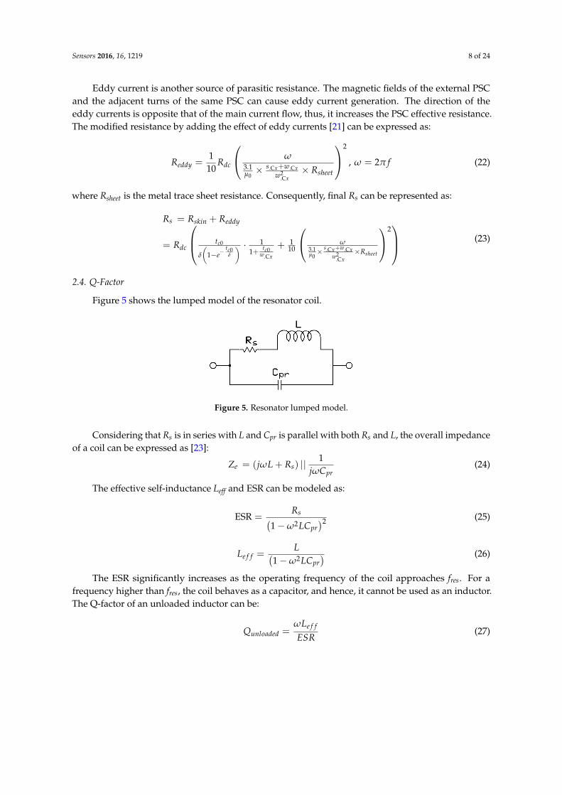
2.4. Q-Factor

Figure 5 shows the lumped model of the resonator coil.

Sensors 2016, 16, 1219 8 of 24

Eddy current is another source of parasitic resistance. The magnetic fields of the external PSC and the adjacent turns of the same PSC can cause eddy current generation. The direction of the eddy currents is opposite that of the main current flow, thus, it increases the PSC effective resistance. The modified resistance by adding the effect of eddy currents [21] can be expressed as:

2

.C .C2

0 .C

1, 2

3.110eddy dcx x

sheetx

R R fs w Rw

(22)

where Rsheet is the metal trace sheet resistance. Consequently, final Rs can be represented as:

0

2

0

0 .C .C2

.C 0 .C

1 13.11011

c

s skin eddy

cdc t

c x xsheet

x x

R R R

tR t s w Re w w

(23)

2.4. Q-Factor

Figure 5 shows the lumped model of the resonator coil.

Figure 5. Resonator lumped model.

Considering that Rs is in series with L and Cpr is parallel with both Rs and L, the overall impedance of a coil can be expressed as [23]:

1

e s

pr

Z j L Rj C

(24)

The effective self-inductance Leff and ESR can be modeled as:

22ESR

1

s

pr

R

LC

(25)

21

eff

pr

LLLC

(26)

The ESR significantly increases as the operating frequency of the coil approaches fres. For a frequency higher than fres, the coil behaves as a capacitor, and hence, it cannot be used as an inductor. The Q-factor of an unloaded inductor can be:

eff

unloaded

LQ

ESR (27)

2.5. Power Transfer Efficiency

By applying the circuit theory to Figure 6, the relationship between the current through each coil and the voltage applied to the source can be expressed in the following matrix form [23]:

Figure 5. Resonator lumped model.

Considering that Rs is in series with L and Cpr is parallel with both Rs and L, the overall impedanceof a coil can be expressed as [23]:

Ze = (jωL + Rs) ||1

jωCpr(24)

The effective self-inductance Leff and ESR can be modeled as:

ESR =Rs(

1−ω2LCpr)2 (25)

Le f f =L(

1−ω2LCpr) (26)

The ESR significantly increases as the operating frequency of the coil approaches fres. For afrequency higher than fres, the coil behaves as a capacitor, and hence, it cannot be used as an inductor.The Q-factor of an unloaded inductor can be:

Qunloaded =ωLe f f

ESR(27)

Sensors 2016, 16, 1219 9 of 24

2.5. Power Transfer Efficiency

By applying the circuit theory to Figure 6, the relationship between the current through each coiland the voltage applied to the source can be expressed in the following matrix form [23]:

I1

I2

I3

I4

=

Z11 Z12 Z13 Z14

Z21 Z22 Z23 Z24

Z31 Z32 Z33 Z34

Z41 Z42 Z43 Z44

−1

E000

(28)

Sensors 2016, 16, 1219 9 of 24

1

11 12 13 141

21 22 23 242

3 31 32 33 34

4 41 42 43 44

0

0

0

Z Z Z ZI EZ Z Z ZI

I Z Z Z ZI Z Z Z Z

(28)

Figure 6. Simplified electric model of the four -coil PTE system.

Equation (28) can be further expanded as [35–37]:

1 1 12 13 14

21 2 2 23 24

2

31 31 3 3 34

3

41 42 43 4 4

1

1

1

2

3

4

4

1

1

1

0

0

0

1

src

load

R R j L j M j M j M

j M R j L j M j Mj C

j M j M R j L j Mj C

j M j M j M R R j L

j CI EIII

j C

(29)

where Rsrc is the source resistance and Rload is the load resistance. Rsrc and R4 are small in magnitude, and at resonant frequency, jωL = 1/jωC. Hence, the imaginary part of the corresponding element is zero. C1 and C4 are small in size; thus, they have a very small inductance and can be neglected. The large distances between C1 and C4, C1 and C3, and C2 and C4 result insignificant mutual inductance and mutual resistance [23,35,38]. Therefore a simplified form of Equation (29) can be expressed as:

1 12

21 2 23

31 3 34

43

1

2

3

4

10 0

0

0

0 0

0

0

0

load

R j M

j M R j M

j M R j M

j M R

I EIII

(30)

To simplify PTE equation, Mij is usually normalized by using Li and Lj by defining kc.ij as:

. ijc ij

i j

Mk

L L (31)

At resonance, PTE η can be expressed as: 24

1

Output Power

Input Power loadI R

I E (32)

For loaded Q-factor Q4L, Equation (32) can be expanded as [39]:

Figure 6. Simplified electric model of the four -coil PTE system.

Equation (28) can be further expanded as [35–37]:

I1

I2

I3

I4

=

Rsrc + R1 + jωL1 +

1jωC1

jωM12 jωM13 jωM14

jωM21 R2 + jωL2 +1

jωC2jωM23 jωM24

jωM31 jωM31 R3 + jωL3 +1

jωC3jωM34

jωM41 jωM42 jωM43 Rload + R4 + jωL4 +1

jωC4

−1 E000

(29)

where Rsrc is the source resistance and Rload is the load resistance. Rsrc and R4 are small in magnitude,and at resonant frequency, jωL = 1/jωC. Hence, the imaginary part of the corresponding element is zero.C1 and C4 are small in size; thus, they have a very small inductance and can be neglected. The largedistances between C1 and C4, C1 and C3, and C2 and C4 result insignificant mutual inductance andmutual resistance [23,35,38]. Therefore a simplified form of Equation (29) can be expressed as:

I1

I2

I3

I4

=

R1 jωM12 0 0

jωM21 R2 jωM23 0

0 jωM31 R3 jωM34

0 0 jωM43 Rload

−1

E000

(30)

To simplify PTE equation, Mij is usually normalized by using Li and Lj by defining kc.ij as:

kc.ij =Mij√LiLj

(31)

At resonance, PTE η can be expressed as:

η =Output PowerInput Power

=I24 Rload

I1E(32)

Sensors 2016, 16, 1219 10 of 24

For loaded Q-factor Q4L, Equation (32) can be expanded as [39]:

η = η12 × η23 × η34

η =k2

c.12Q1Q2·k2c.23Q2Q3·k2

c.34Q3Q4L [(1 + k2c.12Q1Q2

)·(1 + k2

c.34Q3Q4L)+ k2

c.23Q2Q3]×(

1 + k2c.23Q2Q3 + k2

c.34Q3Q4L) ×

Q4LQL (33)

where QL (=Rload/ωL4) is the load Q-factor and Q4L = (Q4·QL)/(Q4 + QL). The PTE (η23) of looselycoupled C2 and C3 is the dominant factor in determining the overall PTE of the four-coil link atlarge coupling distance d. In Equation (27), the effects of adjacent coils in a multi-coil-based systemare ignored. In contrast, Q-factor can be estimated more accurately by considering the effect ofreflected impedance from the load coil back to the driver coil, one stage at time in a multi-coil system.At resonance, the effect of RX on TX can be modeled using the reflected impedance [40]:

Rre f .j,j+1 = k2c.j,j+1 ωLjQ(j+1)L, j = 1, 2, ... m− 1 (34)

In Equation (34), Rref.j,j+1 represents the reflected load from (j + 1)th to jth coil, where kc.j,j+1 is thecoupling coefficient between the jth and (j + 1)th coils and all coils are tuned at fres. Q(j+1)L is the loadedQ-factor of the (j + 1)th coil, which can be obtained from:

QjL =ωLj

Rj + Rre f .j,(j+1)=

ωLjRj

1 + k2c.j,j+1

(ωLjRj

)Q(j+1)L

=Qj

1 + k2c.j,j+1QjQ(j+1)L

(35)

where, Qj = Qunloaded = (ωLj/Rj) and Rj are the unloaded quality factor Equation (27) and parasiticseries resistance of the jth coil, respectively. According to Equation (34), when RLoad is reflected ontoC3 through C4, it limits the Q-factor of C3 [40]. Similarly, the total impedance in the secondary coil(C3) is reflected onto the primary coil (C2) and reduces the Q-factor of C2 (Q2 = ωL2/R2), which can beexpressed as:

Q2L =Q2

1 + k2c.23Q2Q3L

(36)

From Equation (36) it can be inferred that strong coupling between C2 and C3 (i.e., high kc.23)reduces Q2L and thus, η12, which is the PTE between C1 and C2. In Equation (36) Q2L is roughlyproportional to kc.23

−2, where kc.23 is further inversely proportional to d2 [23]. Therefore, Q2L isproportional to d4. For a small d, Q2L will reduce significantly. It implies that η12 will reduce enormouslyas well. η12 can be expressed as [40]:

η12 =k2

c.12Q1Q2L

1 + k2c.12Q1Q2L

× Q2LQL

(37)

In Equation (37), η12 is significantly reduced at small d if kc.12 is not chosen to be large. According toEquation (34), large kc.12 results in a large reflected load on C1, which can reduce the available powerfrom the source. On the other hand, PDL Pload can be calculated by multiplying the power provided bypower source E by the PTE as [40]:

Pload =E2

2Rre f .1,2× η (38)

3. Design and Optimization Procedure

In this section, the design steps for a fully planar four-coil MRC WPT are presented usingthe theoretical models of Section 2. These steps are presented in the context of optimizing thedesign constraints and achieving maximum PTE with an utilizable PDL for implantable device.A MATLAB model of Equations (1)~(33) is developed and used to optimize the architecture of the coils

Sensors 2016, 16, 1219 11 of 24

to achieve high PTE. The parasitic modeling are also utilized to engender appropriate optimization.The high-frequency structure simulator ANSYS-HFSS-15.0 with circuit modeling and the simulationsoftware ANSYS-Simplorer is used to simulate and validate the optimization of the size of the TX andRX coils.

3.1. Design Constraints

The first step is to specify the design parameters of the four-coil WPT system for biomedicalimplants. Table 1 lists the design constraints in terms of the size, coupling distance, fabricationtechnology, carrier frequency, and load resistance.

Table 1. Design Constraints.

Parameters Symbol Design Value

TX outer diameter Dout.C2 ≤60 mmRX outer diameter Dout.C3 ≤20 mm

Coil thickness tc0 38 µmConductor material properties ρc, µr ~17 nΩm, ~1

Substrate thickness tc7 1.6 mmSubstrate dielectric constant εr7 4.4 (FR4)

Link operating frequency fres 13.56 MHzCoil relative thickness d 10 mm

Load resistance Rload 100 Ω

3.2. Parameter Initialization

Before the iterative optimization process is started, a set of values are needed to be initialized.To realize a high PTE in a relatively compact structure, the design initialization starts with the couplingcoefficient (kc.23) [23,41]. It is a generalized approximation for both square and circular coils:

kc.23 = 148.2(

1d2 + r2

m

)1.2− 0.0002857 (39)

where rm is the geometric mean of the radius of the TX and RX coils. From Equation (39) and Table 1,the estimated kc.23 is 0.1182 when d = 10 mm, which is shown in Figure 7.

Sensors 2016, 16, 1219 11 of 24

high PTE. The parasitic modeling are also utilized to engender appropriate optimization. The high-frequency structure simulator ANSYS-HFSS-15.0 with circuit modeling and the simulation software ANSYS-Simplorer is used to simulate and validate the optimization of the size of the TX and RX coils.

3.1. Design Constraints

The first step is to specify the design parameters of the four-coil WPT system for biomedical implants. Table 1 lists the design constraints in terms of the size, coupling distance, fabrication technology, carrier frequency, and load resistance.

Table 1. Design Constraints.

Parameters Symbol Design Value

TX outer diameter Dout.C2 ≤60 mm RX outer diameter Dout.C3 ≤20 mm

Coil thickness tc0 38 µm Conductor material properties ρc, µr ~17 nΩm, ~1

Substrate thickness tc7 1.6 mm Substrate dielectric constant ɛr7 4.4 (FR4)

Link operating frequency fres 13.56 MHz Coil relative thickness d 10 mm

Load resistance Rload 100 Ω

3.2. Parameter Initialization

Before the iterative optimization process is started, a set of values are needed to be initialized. To realize a high PTE in a relatively compact structure, the design initialization starts with the coupling coefficient (kc.23) [23,41]. It is a generalized approximation for both square and circular coils:

1.2

.23 2 2

1148.2 0.0002857

cm

kd r

(39)

where rm is the geometric mean of the radius of the TX and RX coils. From Equation (39) and Table 1, the estimated kc.23 is 0.1182 when d = 10 mm, which is shown in Figure 7.

Figure 7. Mutual coupling (kc.23) versus distance.

Figure 7. Mutual coupling (kc.23) versus distance.

Sensors 2016, 16, 1219 12 of 24

The maximum achievable PTE in Equation (33) at a 10-mm relative distance between the TX andRX coils is 84% for the specified kc.23 value. Figure 8 shows that the maximum PTE is achieved forC2 Q-factor Q2 = 226. The minimum necessary Q-factor for C1 and C4 can be approximated fromQ1,4 > Q−0.5

2,3 . The coupling coefficients and Q-factors of C1, C3, and C4 in Equation (33) are initialized,as listed in Table 2. It lists the parameters [22,23,27] that are iteratively optimized by using MATLAB inthe further parts of this paper to achieve maximum PTE. Simultaneously, the optimized architecture isvalidated using HFSS. Based on the initial values of Table 2 the TX and RX coils are modeled in HFSS.In order to reduce the power losses in transmission load, copper material with 0.038 mm thickness isprinted on FR4-epoxy substrate with constitutive parameters of 1.6 mm substrate thickness, 4.4 relativepermittivity (εr), 0.02 dielectric loss tangent, and “1” relative permeability (µr). Resonant circuit similarto Figure 6 is modeled and simulated in Simplorer to measure the PTE of the HFSS modeled coils atthe operating frequency of 13.56 MHz.

Sensors 2016, 16, 1219 12 of 24

The maximum achievable PTE in Equation (33) at a 10-mm relative distance between the TX and RX coils is 84% for the specified kc.23 value. Figure 8 shows that the maximum PTE is achieved for C2 Q-factor Q2 = 226. The minimum necessary Q-factor for C1 and C4 can be approximated from , , . . The coupling coefficients and Q-factors of C1, C3, and C4 in Equation (33) are initialized, as listed in Table 2. It lists the parameters [22,23,27] that are iteratively optimized by using MATLAB in the further parts of this paper to achieve maximum PTE. Simultaneously, the optimized architecture is validated using HFSS. Based on the initial values of Table 2 the TX and RX coils are modeled in HFSS. In order to reduce the power losses in transmission load, copper material with 0.038 mm thickness is printed on FR4-epoxy substrate with constitutive parameters of 1.6 mm substrate thickness, 4.4 relative permittivity (ɛr), 0.02 dielectric loss tangent, and “1” relative permeability (µr). Resonant circuit similar to Figure 6 is modeled and simulated in Simplorer to measure the PTE of the HFSS modeled coils at the operating frequency of 13.56 MHz.

Figure 8. Efficiency versus Q-factor versus distance.

Table 2. Initial Values.

Parameters Symbol Value

C1 inner diameter Din.C1 20 mm C4 inner diameter Din.C4 8 mm

C1 line width w.C1 2 mm C1 line spacing s.C1 150 µm C2 line width w.C2 (minimum) 150 µm

C2 line spacing s.C2 (minimum) 150 µm C3 line width w.C3 (minimum) 150 µm

C3 line spacing s.C3 (minimum) 150 µm C4 line width w.C4 2 mm

C4 line spacing s.C4 150 µm C1 number of turns n.C1 1 C4 number of turns n.C4 1

C1 Q-factor Q1 4 C3 Q-factor Q3 120 C4 Q-factor Q4 1.4

C1 & C2 coupling coefficient kc.12 0.5

Figure 8. Efficiency versus Q-factor versus distance.

Table 2. Initial Values.

Parameters Symbol Value

C1 inner diameter Din.C1 20 mmC4 inner diameter Din.C4 8 mm

C1 line width w.C1 2 mmC1 line spacing s.C1 150 µmC2 line width w.C2 (minimum) 150 µm

C2 line spacing s.C2 (minimum) 150 µmC3 line width w.C3 (minimum) 150 µm

C3 line spacing s.C3 (minimum) 150 µmC4 line width w.C4 2 mm

C4 line spacing s.C4 150 µmC1 number of turns n.C1 1C4 number of turns n.C4 1

C1 Q-factor Q1 4C3 Q-factor Q3 120C4 Q-factor Q4 1.4

C1 & C2 coupling coefficient kc.12 0.5C3 & C4 coupling coefficient kc.34 0.45

Sensors 2016, 16, 1219 13 of 24

3.3. Size and Number of Turns of Primary PSC

To optimize the size of the primary PSC, the values approximated in steps 1 and 2 are used inEquations (1)~(33). By keeping s and w constant, Dout.C2 and n.C2 are swept in a wide range aroundtheir initial values to extract the highest PTE. According to [22], n.C2 can be expressed as a functionof ϕ2:

n.C2 =Dout.C2

s.C2 + w.C2· ϕ2

(1 + ϕ2)(40)

For a square-shaped coil, Figure 9a shows that the best choice for Dout.C2 is 40 mm. The maximumPTE is 59.66% when the number of turns n.C2 = 12. The PTE should improve once w.C2 and the sizeof the secondary PSC are optimized. Similarly, the circular coil shown in Figure 9b reaches its peakη = 57.84% at Dout.C2 = 38.5 mm and n.C2 = 11.5. Figure 9c shows calculated and simulated values ofPTE versus n.C2 at Dout.C2 = 40 mm for square coil. Similarly, Figure 9d shows calculated and simulatedvalues of PTE versus n.C2 at Dout.C2 = 38.5 mm for circular coil.

Sensors 2016, 16, 1219 13 of 24

3.3. Size and Number of Turns of Primary PSC

To optimize the size of the primary PSC, the values approximated in steps 1 and 2 are used in Equations (1)~(33). By keeping s and w constant, Dout.C2 and n.C2 are swept in a wide range around their initial values to extract the highest PTE. According to [22], n.C2 can be expressed as a function of φ2:

.C 2 2.C 2

.C 2 .C 2 2(1 )

outDn

s w (39)

For a square-shaped coil, Figure 9a shows that the best choice for Dout.C2 is 40 mm. The maximum PTE is 59.66% when the number of turns n.C2 = 12. The PTE should improve once w.C2 and the size of the secondary PSC are optimized. Similarly, the circular coil shown in Figure 9b reaches its peak η = 57.84% at Dout.C2 = 38.5 mm and n.C2 = 11.5. Figure 9c shows calculated and simulated values of PTE versus n.C2 at Dout.C2 = 40 mm for square coil. Similarly, Figure 9d shows calculated and simulated values of PTE versus n.C2 at Dout.C2 = 38.5 mm for circular coil.

(a) (b)

(c) (d)

Figure 9. Optimization of the size and number of turns of the primary PSC. (a) Efficiency versus outer diameter versus number of turns of the square coil; (b) Efficiency versus outer diameter versus number of turns of the circular coil; (c) Calculated and simulated efficiency versus number of turns of the square coil; (d) Calculated and simulated efficiency versus number of turns of the circular coil.

3.4. Fill Factor and Line Width of Secondary PSC

After temporarily fixing the parameters of the primary PSC in the previous step, the next step generalizes the structure parameters of the secondary coil. Considering that Dout.C3 is predetermined in the design constraints, in this step, φ3 is swept around its nominal value and increases w.C3 from its minimum value. Figure 10a shows that the maximum PTE of a square PSC is slightly below the specified minimum value of w.C3. Thus, the selected value of the secondary PSC line width is

Figure 9. Optimization of the size and number of turns of the primary PSC. (a) Efficiency versus outerdiameter versus number of turns of the square coil; (b) Efficiency versus outer diameter versus numberof turns of the circular coil; (c) Calculated and simulated efficiency versus number of turns of the squarecoil; (d) Calculated and simulated efficiency versus number of turns of the circular coil.

3.4. Fill Factor and Line Width of Secondary PSC

After temporarily fixing the parameters of the primary PSC in the previous step, the next stepgeneralizes the structure parameters of the secondary coil. Considering that Dout.C3 is predeterminedin the design constraints, in this step, ϕ3 is swept around its nominal value and increases w.C3 fromits minimum value. Figure 10a shows that the maximum PTE of a square PSC is slightly belowthe specified minimum value of w.C3. Thus, the selected value of the secondary PSC line width is

Sensors 2016, 16, 1219 14 of 24

w.C3 = w.C3 (minimum). According to the initialized value, Din.C3 = 12.3 mm. Therefore, to manage thesize constraints and maximum PTE trade-off, we select ϕ3 = 0.24, which corresponds to n.C3 = 12.9 andyields η = 83%.

Sensors 2016, 16, 1219 14 of 24

w.C3 = w.C3 (minimum). According to the initialized value, Din.C3 = 12.3 mm. Therefore, to manage the size constraints and maximum PTE trade-off, we select φ3 = 0.24, which corresponds to n.C3 = 12.9 and yields η = 83%.

Similar to the square secondary PSC parameters, Figure 10b shows the approximation of the parameters of the circular secondary PSC. Maximum PTE η = 82.19% can be achieved for w.C3 = w.C3(minimum) by considering the size constraints as well as the initial values. To obtain the peak PTE we select φ3 = 0.26, which yields n.C3 = 13.75. Figure 10c shows calculated and simulated values of PTE versus w.C3 at φ3 = 0.24 for the square coil. Similarly, Figure 10d shows calculated and simulated values of PTE versus w.C3 at φ3 = 0.26 for the circular coil.

(a) (b)

(c) (d)

Figure 10. Optimization of the trace line width and fill factor of the secondary PSC. (a) Efficiency versus line width versus fill factor of the square coil; (b) Efficiency versus line width versus fill factor of the circular coil; (c) Calculated and simulated efficiency versus line width of the square coil; (d) Calculated and simulated efficiency versus line width of the circular coil.

3.5. Size and Line Width of Primary PSC

In this step, the conductor width w.C2 is increased toward its optimum value while the outer diameter is also increased to provide room for the excess w.C2. The increase in w.C2 reduces Rs.C2 and increases Q2. Hence, the overall PTE is improved. Figure 11a shows that the PTE reaches its peak η = 86.85%for optimal value of w.C2 = 1.2 mm and Dout.C2 = 57 mm by considering n.C2 = 12, which is obtained from the previous step. Following the same steps for the circular PSC, Figure 11b shows the peak PTE at η = 85.01% for w.C2 = 1.05 mm and Dout.C2 = 52 mm. The number of turns is fixed at n.C2 = 11.5, which is extracted from the previous step. Figure 11c shows calculated and simulated values of PTE versus Dout.C2 at w.C2 = 1.2 mm for the square coil. Similarly, Figure 11d shows calculated and simulated values of PTE versus Dout.C2 at w.C2 = 1.05 mm for the circular coil.

Figure 10. Optimization of the trace line width and fill factor of the secondary PSC. (a) Efficiency versusline width versus fill factor of the square coil; (b) Efficiency versus line width versus fill factorof the circular coil; (c) Calculated and simulated efficiency versus line width of the square coil;(d) Calculated and simulated efficiency versus line width of the circular coil.

Similar to the square secondary PSC parameters, Figure 10b shows the approximation ofthe parameters of the circular secondary PSC. Maximum PTE η = 82.19% can be achieved forw.C3 = w.C3(minimum) by considering the size constraints as well as the initial values. To obtain the peakPTE we select ϕ3 = 0.26, which yields n.C3 = 13.75. Figure 10c shows calculated and simulated values ofPTE versus w.C3 at ϕ3 = 0.24 for the square coil. Similarly, Figure 10d shows calculated and simulatedvalues of PTE versus w.C3 at ϕ3 = 0.26 for the circular coil.

3.5. Size and Line Width of Primary PSC

In this step, the conductor width w.C2 is increased toward its optimum value while the outerdiameter is also increased to provide room for the excess w.C2. The increase in w.C2 reduces Rs.C2 andincreases Q2. Hence, the overall PTE is improved. Figure 11a shows that the PTE reaches its peakη = 86.85% for optimal value of w.C2 = 1.2 mm and Dout.C2 = 57 mm by considering n.C2 = 12, whichis obtained from the previous step. Following the same steps for the circular PSC, Figure 11b showsthe peak PTE at η = 85.01% for w.C2 = 1.05 mm and Dout.C2 = 52 mm. The number of turns is fixedat n.C2 = 11.5, which is extracted from the previous step. Figure 11c shows calculated and simulatedvalues of PTE versus Dout.C2 at w.C2 = 1.2 mm for the square coil. Similarly, Figure 11d shows calculatedand simulated values of PTE versus Dout.C2 at w.C2 = 1.05 mm for the circular coil.

Sensors 2016, 16, 1219 15 of 24Sensors 2016, 16, 1219 15 of 24

(a) (b)

(c) (d)

Figure 11. Optimization of the trace line width and size of the primary PSC. (a) Efficiency versus line width versus outer diameter of the square coil; (b) Efficiency versus line width versus outer diameter of the circular coil; (c) Calculated and simulated efficiency versus outer diameter of the square coil; (d) Calculated and simulated efficiency versus outer diameter of the circular coil.

3.6. Iteration and Validation

The previous step shows that by updating the geometric size, the PTE can be significantly improved. On the other hand, further improvement is possible by iterating the whole optimization procedure. To achieve higher efficiency, some parameters (Din.C1, Din.C4, w.C1, w.C4, and s) are also adjusted during simulation in HFSS. The iteration process can be continued until the improvement in PTE per iteration is less than 0.2%. Table 3 lists the final optimized geometric values, and Figure 12 shows the summary of the iterative PSC design procedures in a flowchart form.

Table 3. Optimized Geometric Values.

Parameters Square Coil Circular Coil Parameters Square Coil Circular Coil

Din.C1 (mm) 24 24 w.C2 (mm) 1.24 1.21

Dout.C1 (mm) 32 32 s.C2 (µm) 150 150

Din.C2 (mm) 32.3 32.6 w.C3 (µm) 170 150

Dout.C2 (mm) 65.5 65 s.C3 (µm) 150 150

Din.C3 (mm) 13.9 14 w.C4 (mm) 1.8 1.8

Dout.C3 (mm) 20.5 20.3 s.C4 (µm) 150 200

Din.C4 (mm) 10 10 n.C1 1 1

Dout.C4 (mm) 13.6 13.6 n.C2 12 12

w.C1 (mm) 4 4 n.C3 10 10

s.C1 (µm) 150 300 n.C4 1 1

Figure 11. Optimization of the trace line width and size of the primary PSC. (a) Efficiency versus linewidth versus outer diameter of the square coil; (b) Efficiency versus line width versus outer diameterof the circular coil; (c) Calculated and simulated efficiency versus outer diameter of the square coil;(d) Calculated and simulated efficiency versus outer diameter of the circular coil.

3.6. Iteration and Validation

The previous step shows that by updating the geometric size, the PTE can be significantlyimproved. On the other hand, further improvement is possible by iterating the whole optimizationprocedure. To achieve higher efficiency, some parameters (Din.C1, Din.C4, w.C1, w.C4, and s) are alsoadjusted during simulation in HFSS. The iteration process can be continued until the improvement inPTE per iteration is less than 0.2%. Table 3 lists the final optimized geometric values, and Figure 12shows the summary of the iterative PSC design procedures in a flowchart form.

Table 3. Optimized Geometric Values.


Din.C1 (mm) 24 24 w.C2 (mm) 1.24 1.21Dout.C1 (mm) 32 32 s.C2 (µm) 150 150Din.C2 (mm) 32.3 32.6 w.C3 (µm) 170 150Dout.C2 (mm) 65.5 65 s.C3 (µm) 150 150Din.C3 (mm) 13.9 14 w.C4 (mm) 1.8 1.8Dout.C3 (mm) 20.5 20.3 s.C4 (µm) 150 200Din.C4 (mm) 10 10 n.C1 1 1Dout.C4 (mm) 13.6 13.6 n.C2 12 12

w.C1 (mm) 4 4 n.C3 10 10s.C1 (µm) 150 300 n.C4 1 1

Sensors 2016, 16, 1219 16 of 24Sensors 2016, 16, 1219 16 of 24

Figure 12. Iterative design flowchart.

4. Fabrication and Results

To verify the accuracy of the PTE and PDL equations through measurement, both the square and circular fully planar four-coil MRC-WPTs are fabricated on 1.6-mm-thick FR4 printed circuit boards. Figure 13a,b shows the fabricated square and circular coils, respectively. For a nominal coupling distance of d = 10 mm, Rload = 100 Ω, and f = 13.56 MHz, Table 4 lists the electrical specifications of the designed coils achieved from simulation.

Figure 14 shows the experimental setup [35] to verify the fabricated coils. Resonant circuit similar to Figure 6 is built for both the square and circular coils. A signal generator is used as a power source and Rsrc = 50 Ω. For the measurement, an oscilloscope (DPO 4034, Tektronics, Beaverton, OR, USA) and an LCR meter are used. The transmitted and received power can be easily determined by measuring the current and voltage waveforms.

(a)

Figure 13. Cont.



To verify the accuracy of the PTE and PDL equations through measurement, both the square andcircular fully planar four-coil MRC-WPTs are fabricated on 1.6-mm-thick FR4 printed circuit boards.Figure 13a,b shows the fabricated square and circular coils, respectively. For a nominal couplingdistance of d = 10 mm, Rload = 100 Ω, and f = 13.56 MHz, Table 4 lists the electrical specifications of thedesigned coils achieved from simulation.

Table 4. Electrical Specification.


L1 (nH) 78.78 67.6 Q1 2.55 2.44L2 (µH) 9.25 8.03 Q2 313.6 302.7L3 (µH) 3.09 2.59 Q3 97.76 92.32L4 (nH) 44.07 50.1 Q4 (loaded) 0.84 0.82C1 (nF) 1.76 2.04 kc.12 0.32 0.287C2 (pF) 14.9 17.16 kc.23 0.112 0.11C3 (pF) 44.5 53.2 kc.34 0.33 0.27C4 (nF) 3.13 2.75 M23 (nH) 594.6 504.06R1 (Ω) 0.05 0.047 d (mm) 10 10R2 (Ω) 2.51 2.26 η (simulated) 81.66% 79.07%R3 (Ω) 2.82 2.39 η (measured) 79.8% 78.43%R4 (Ω) 0.04 0.052

Sensors 2016, 16, 1219 17 of 24

Sensors 2016, 16, 1219 16 of 24



To verify the accuracy of the PTE and PDL equations through measurement, both the square and circular fully planar four-coil MRC-WPTs are fabricated on 1.6-mm-thick FR4 printed circuit boards. Figure 13a,b shows the fabricated square and circular coils, respectively. For a nominal coupling distance of d = 10 mm, Rload = 100 Ω, and f = 13.56 MHz, Table 4 lists the electrical specifications of the designed coils achieved from simulation.

Figure 14 shows the experimental setup [35] to verify the fabricated coils. Resonant circuit similar to Figure 6 is built for both the square and circular coils. A signal generator is used as a power source and Rsrc = 50 Ω. For the measurement, an oscilloscope (DPO 4034, Tektronics, Beaverton, OR, USA) and an LCR meter are used. The transmitted and received power can be easily determined by measuring the current and voltage waveforms.

(a)

Figure 13. Cont.

Sensors 2016, 16, 1219 17 of 24

(b)

Figure 13. Coil dimension. (a) Square coil. (b) Circular coil.



L1 (nH) 78.78 67.6 Q1 2.55 2.44 L2 (µH) 9.25 8.03 Q2 313.6 302.7 L3 (µH) 3.09 2.59 Q3 97.76 92.32 L4 (nH) 44.07 50.1 Q4(loaded) 0.84 0.82 C1 (nF) 1.76 2.04 kc.12 0.32 0.287 C2 (pF) 14.9 17.16 kc.23 0.112 0.11 C3 (pF) 44.5 53.2 kc.34 0.33 0.27 C4 (nF) 3.13 2.75 M23(nH) 594.6 504.06 R1 (Ω) 0.05 0.047 d (mm) 10 10 R2 (Ω) 2.51 2.26 η (simulated) 81.66% 79.07% R3 (Ω) 2.82 2.39 η (measured) 79.8% 78.43% R4 (Ω) 0.04 0.052

(a)

(b)

Figure 14. Experimental setup. (a) Square coil; (b) Circular coil.


Figure 14 shows the experimental setup [35] to verify the fabricated coils. Resonant circuit similarto Figure 6 is built for both the square and circular coils. A signal generator is used as a power sourceand Rsrc = 50 Ω. For the measurement, an oscilloscope (DPO 4034, Tektronics, Beaverton, OR, USA) andan LCR meter are used. The transmitted and received power can be easily determined by measuringthe current and voltage waveforms.

Sensors 2016, 16, 1219 17 of 24

(b)




L1 (nH) 78.78 67.6 Q1 2.55 2.44 L2 (µH) 9.25 8.03 Q2 313.6 302.7 L3 (µH) 3.09 2.59 Q3 97.76 92.32 L4 (nH) 44.07 50.1 Q4(loaded) 0.84 0.82 C1 (nF) 1.76 2.04 kc.12 0.32 0.287 C2 (pF) 14.9 17.16 kc.23 0.112 0.11 C3 (pF) 44.5 53.2 kc.34 0.33 0.27 C4 (nF) 3.13 2.75 M23(nH) 594.6 504.06 R1 (Ω) 0.05 0.047 d (mm) 10 10 R2 (Ω) 2.51 2.26 η (simulated) 81.66% 79.07% R3 (Ω) 2.82 2.39 η (measured) 79.8% 78.43% R4 (Ω) 0.04 0.052

(a)

(b)

Figure 14. Experimental setup. (a) Square coil; (b) Circular coil. Figure 14. Experimental setup. (a) Square coil; (b) Circular coil.

Figure 15 shows the comparison of the calculated, simulated, and measured values of the PTEversus coupling distance in the square and circular coil inductive links. The designed coils are

Sensors 2016, 16, 1219 18 of 24

optimized for 10 mm of coupling distance and generate a maximum PTE at that specified couplingdistance. High Rsrc is an important factor to degrade the PTE performance from the MATLABsimulation to HFSS simulation and measurement data. During MATLAB simulation of PTE inEquation (33) the effect of kc.14, kc.24, and kc.13 are neglected. At d < 5 mm, these parameters cannotbe neglected. The effect of Rsrc in Equation (30) is not considered as well for the simplicity of thecalculation and simulation in MATLAB. Thus, there is a discrepancy visible between the calculation(MATLAB simulation) and measured data (HFSS simulation and measured) at d < 5 mm.

Sensors 2016, 16, 1219 18 of 24

Figure 15 shows the comparison of the calculated, simulated, and measured values of the PTE versus coupling distance in the square and circular coil inductive links. The designed coils are optimized for 10 mm of coupling distance and generate a maximum PTE at that specified coupling distance. High Rsrc is an important factor to degrade the PTE performance from the MATLAB simulation to HFSS simulation and measurement data. During MATLAB simulation of PTE in Equation (33) the effect of kc.14, kc.24, and kc.13 are neglected. At d < 5 mm, these parameters cannot be neglected. The effect of Rsrc in Equation (30) is not considered as well for the simplicity of the calculation and simulation in MATLAB. Thus, there is a discrepancy visible between the calculation (MATLAB simulation) and measured data (HFSS simulation and measured) at d < 5 mm.

Figure 15. Efficiency versus coupling distance.

For a frequency sweep of 500 Hz to 30 MHz, the PTE is maximized at approximately 13–14 MHz because of the high Q-factor of the PSCs for both the square and circular coils, as shown in Figure 16. The improvement in PTE is very small at higher frequencies.

Figure 16. Efficiency versus carrier frequency.

Figure 17 shows the effect of lateral misalignment on PTE. The variation of PTE for Equation (4) is simulated using MATLAB and verified by HFSS simulation and measurement. TX coil is kept constant and RX coil's positions are changed from 0 mm to 20 mm lateral plane for both simulation and experimental measurement at d = 10 mm. The PTE decreases significantly for higher lateral displacement of the RX coil. The effect of angular misalignment on PTE is observed for MATLAB simulation, HFSS simulation, and practical measurement on Figure 18. For d = 20 mm the PTE is


For a frequency sweep of 500 Hz to 30 MHz, the PTE is maximized at approximately 13–14 MHzbecause of the high Q-factor of the PSCs for both the square and circular coils, as shown in Figure 16.The improvement in PTE is very small at higher frequencies.

Sensors 2016, 16, 1219 18 of 24

Figure 15 shows the comparison of the calculated, simulated, and measured values of the PTE versus coupling distance in the square and circular coil inductive links. The designed coils are optimized for 10 mm of coupling distance and generate a maximum PTE at that specified coupling distance. High Rsrc is an important factor to degrade the PTE performance from the MATLAB simulation to HFSS simulation and measurement data. During MATLAB simulation of PTE in Equation (33) the effect of kc.14, kc.24, and kc.13 are neglected. At d < 5 mm, these parameters cannot be neglected. The effect of Rsrc in Equation (30) is not considered as well for the simplicity of the calculation and simulation in MATLAB. Thus, there is a discrepancy visible between the calculation (MATLAB simulation) and measured data (HFSS simulation and measured) at d < 5 mm.


For a frequency sweep of 500 Hz to 30 MHz, the PTE is maximized at approximately 13–14 MHz because of the high Q-factor of the PSCs for both the square and circular coils, as shown in Figure 16. The improvement in PTE is very small at higher frequencies.


Figure 17 shows the effect of lateral misalignment on PTE. The variation of PTE for Equation (4) is simulated using MATLAB and verified by HFSS simulation and measurement. TX coil is kept constant and RX coil's positions are changed from 0 mm to 20 mm lateral plane for both simulation and experimental measurement at d = 10 mm. The PTE decreases significantly for higher lateral displacement of the RX coil. The effect of angular misalignment on PTE is observed for MATLAB simulation, HFSS simulation, and practical measurement on Figure 18. For d = 20 mm the PTE is


Figure 17 shows the effect of lateral misalignment on PTE. The variation of PTE for Equation (4)is simulated using MATLAB and verified by HFSS simulation and measurement. TX coil is keptconstant and RX coil’s positions are changed from 0 mm to 20 mm lateral plane for both simulationand experimental measurement at d = 10 mm. The PTE decreases significantly for higher lateraldisplacement of the RX coil. The effect of angular misalignment on PTE is observed for MATLAB

Sensors 2016, 16, 1219 19 of 24

simulation, HFSS simulation, and practical measurement on Figure 18. For d = 20 mm the PTE issimulated and measured for λ = 0 to 13 degree. The PTE decreases exponentially in both the cases oflateral and angular misalignments.

Sensors 2016, 16, 1219 19 of 24

simulated and measured for λ = 0 to 13 degree. The PTE decreases exponentially in both the cases of lateral and angular misalignments.

Figure 17. Efficiency versus lateral misalignment.

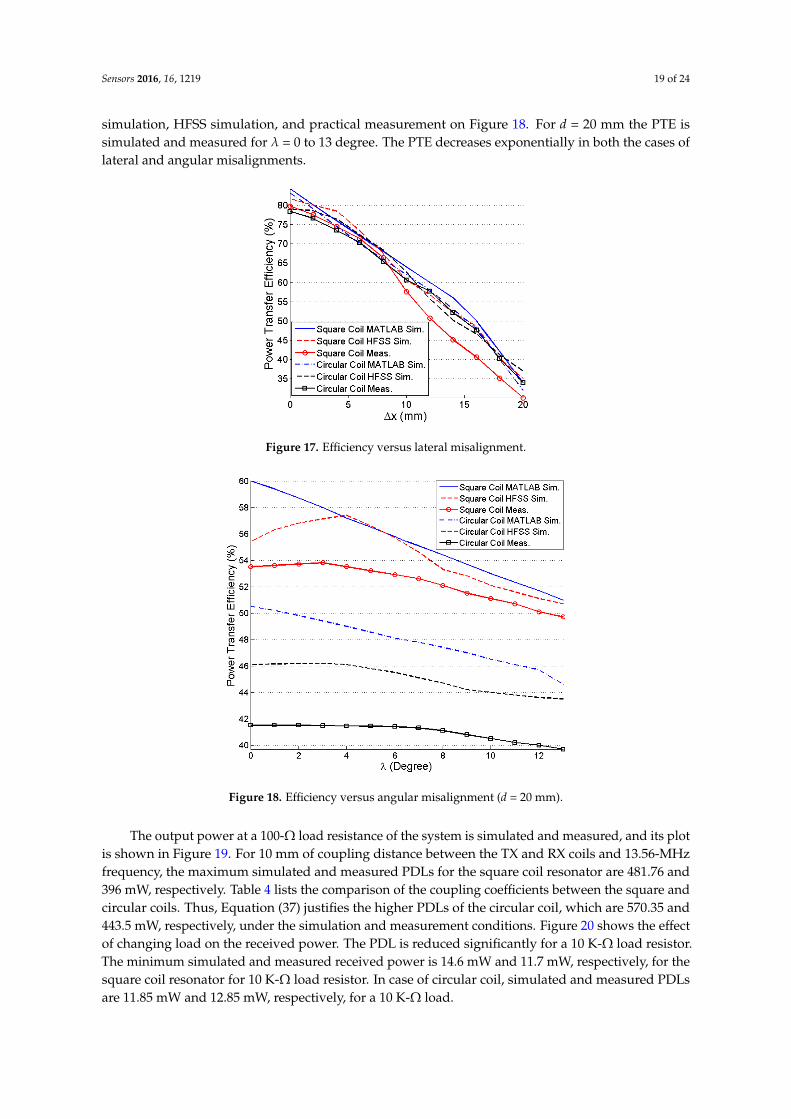
Figure 18. Efficiency versus angular misalignment (d = 20 mm).

The output power at a 100-Ω load resistance of the system is simulated and measured, and its plot is shown in Figure 19. For 10 mm of coupling distance between the TX and RX coils and 13.56-MHz frequency, the maximum simulated and measured PDLs for the square coil resonator are 481.76 and 396 mW, respectively. Table 4 lists the comparison of the coupling coefficients between the square and circular coils. Thus, Equation (37) justifies the higher PDLs of the circular coil, which are 570.35 and 443.5 mW, respectively, under the simulation and measurement conditions. Figure 20 shows the effect of changing load on the received power. The PDL is reduced significantly for a 10 K-Ω load resistor. The minimum simulated and measured received power is 14.6 mW and 11.7 mW, respectively, for the square coil resonator for 10 K-Ω load resistor. In case of circular coil, simulated and measured PDLs are 11.85 mW and 12.85 mW, respectively, for a 10 K-Ω load.


Sensors 2016, 16, 1219 19 of 24

simulated and measured for λ = 0 to 13 degree. The PTE decreases exponentially in both the cases of lateral and angular misalignments.



The output power at a 100-Ω load resistance of the system is simulated and measured, and its plot is shown in Figure 19. For 10 mm of coupling distance between the TX and RX coils and 13.56-MHz frequency, the maximum simulated and measured PDLs for the square coil resonator are 481.76 and 396 mW, respectively. Table 4 lists the comparison of the coupling coefficients between the square and circular coils. Thus, Equation (37) justifies the higher PDLs of the circular coil, which are 570.35 and 443.5 mW, respectively, under the simulation and measurement conditions. Figure 20 shows the effect of changing load on the received power. The PDL is reduced significantly for a 10 K-Ω load resistor. The minimum simulated and measured received power is 14.6 mW and 11.7 mW, respectively, for the square coil resonator for 10 K-Ω load resistor. In case of circular coil, simulated and measured PDLs are 11.85 mW and 12.85 mW, respectively, for a 10 K-Ω load.


The output power at a 100-Ω load resistance of the system is simulated and measured, and its plotis shown in Figure 19. For 10 mm of coupling distance between the TX and RX coils and 13.56-MHzfrequency, the maximum simulated and measured PDLs for the square coil resonator are 481.76 and396 mW, respectively. Table 4 lists the comparison of the coupling coefficients between the square andcircular coils. Thus, Equation (37) justifies the higher PDLs of the circular coil, which are 570.35 and443.5 mW, respectively, under the simulation and measurement conditions. Figure 20 shows the effectof changing load on the received power. The PDL is reduced significantly for a 10 K-Ω load resistor.The minimum simulated and measured received power is 14.6 mW and 11.7 mW, respectively, for thesquare coil resonator for 10 K-Ω load resistor. In case of circular coil, simulated and measured PDLsare 11.85 mW and 12.85 mW, respectively, for a 10 K-Ω load.

Sensors 2016, 16, 1219 20 of 24

Sensors 2016, 16, 1219 20 of 24

Figure 19. PDL versus coupling distance.

Figure 20. PDL versus Rload.

Table 5. Comparison with Previous Work.

Reference Coil Structure Size (Dout.C2, Dout.C3) (mm)

Freq. (MHz)

d (mm)

PTE %

PDL (mW),Rload(Ω)

[27] Fully Planar PSC (50, 50) 13.56 100 77.27 - [42] Planar PSC (120, 120) 50.25 100 43.62 - [26] Fully Planar PSC (53, 53) 160 40 48 - [40] Planar PSC (36.5, 10) 13.56 10 83.5 3.9, 100 [23] Litz Wire (64, 22) 0.7 20 82 75, 100 This

Work Sq. Fully Planar PSC (65.5, 20.5) 13.56 10 79.8 396, 100

This Work

Cir. Fully Planar PSC

(65, 20.3) 13.56 10 78.43 443.5, 100

Table 5 lists the summary and comparison of the work presented in this paper with previous works. The comparison is focused only on the four-coil based resonators for different applications where the coupling medium and surrounding environment is air. Both the square and circular coils are also simulated in a biological tissue medium. In contrast to the air medium, the PTE significantly degrades in the tissue medium. In HFSS, the 10-mm tissue medium is created similar to that shown


Sensors 2016, 16, 1219 20 of 24




Reference Coil Structure Size (Dout.C2, Dout.C3) (mm)

Freq. (MHz)

d (mm)

PTE %

PDL (mW),Rload(Ω)

[27] Fully Planar PSC (50, 50) 13.56 100 77.27 - [42] Planar PSC (120, 120) 50.25 100 43.62 - [26] Fully Planar PSC (53, 53) 160 40 48 - [40] Planar PSC (36.5, 10) 13.56 10 83.5 3.9, 100 [23] Litz Wire (64, 22) 0.7 20 82 75, 100 This

Work Sq. Fully Planar PSC (65.5, 20.5) 13.56 10 79.8 396, 100

This Work

Cir. Fully Planar PSC

(65, 20.3) 13.56 10 78.43 443.5, 100

Table 5 lists the summary and comparison of the work presented in this paper with previous works. The comparison is focused only on the four-coil based resonators for different applications where the coupling medium and surrounding environment is air. Both the square and circular coils are also simulated in a biological tissue medium. In contrast to the air medium, the PTE significantly degrades in the tissue medium. In HFSS, the 10-mm tissue medium is created similar to that shown


Table 5 lists the summary and comparison of the work presented in this paper with previousworks. The comparison is focused only on the four-coil based resonators for different applicationswhere the coupling medium and surrounding environment is air. Both the square and circular coilsare also simulated in a biological tissue medium. In contrast to the air medium, the PTE significantlydegrades in the tissue medium. In HFSS, the 10-mm tissue medium is created similar to that shownin Figure 1, where we consider that the skin, fat, and muscle-tissue thicknesses are 1, 2, and 7 mm,respectively. Table 6 lists the electrical properties of the mentioned human tissues.


Reference Coil Structure Size (Dout.C2, Dout.C3)(mm)

Freq.(MHz)

d(mm)

PTE%

PDL (mW),Rload(Ω)

[27] Fully Planar PSC (50, 50) 13.56 100 77.27 -[42] Planar PSC (120, 120) 50.25 100 43.62 -[26] Fully Planar PSC (53, 53) 160 40 48 -[40] Planar PSC (36.5, 10) 13.56 10 83.5 3.9, 100[23] Litz Wire (64, 22) 0.7 20 82 75, 100

This Work Sq. Fully Planar PSC (65.5, 20.5) 13.56 10 79.8 396, 100This Work Cir. Fully Planar PSC (65, 20.3) 13.56 10 78.43 443.5, 100

Sensors 2016, 16, 1219 21 of 24

Table 6. Human Tissue Electrical Specification (13.56 MHz).

Tissue Type Conductivity (S·m−1) Relative Permittivity

Skin 0.38 177.13Fat 0.03 11.83

Muscle 0.62 138.44

Figure 21 shows the comparison of the simulated and measured PTE of the square and circularPSCs in air and human tissue media under resonance condition. Instead of real human tissue, beeftissue medium was used for the practical measurements. The simulated PTEs of the square and circularcoils are degraded to 55.74% and 38.06%, respectively, when the coupling medium between the TX andRX coils is a three-layered human tissue. Figure 22 shows the experimental setup to measure the PTEwhen the coupling medium between the TX and RX coils is 10 mm of beef muscle tissue, which are cutfrom the lower portion of the ribs. A 20-mm of beef muscle tissue layer is also placed behind the RXcoil. The temperature of the beef muscle was 8.7 C at the time of measurement, and the measured PTEis 48.1% and 35.4%, respectively, for the square and circular PSCs. Due to high permittivity and highconductivity of the biological tissue environment, the Q-factor of each PSC drops significantly. It alsoaffects the parasitic parameters of the PSC. Thus, the PTE is decreased drastically in the biologicaltissue medium than the air medium.

Sensors 2016, 16, 1219 21 of 24

in Figure 1, where we consider that the skin, fat, and muscle-tissue thicknesses are 1, 2, and 7 mm, respectively. Table 6 lists the electrical properties of the mentioned human tissues.



Skin 0.38 177.13 Fat 0.03 11.83

Muscle 0.62 138.44

Figure 21 shows the comparison of the simulated and measured PTE of the square and circular PSCs in air and human tissue media under resonance condition. Instead of real human tissue, beef tissue medium was used for the practical measurements. The simulated PTEs of the square and circular coils are degraded to 55.74% and 38.06%, respectively, when the coupling medium between the TX and RX coils is a three-layered human tissue. Figure 22 shows the experimental setup to measure the PTE when the coupling medium between the TX and RX coils is 10 mm of beef muscle tissue, which are cut from the lower portion of the ribs. A 20-mm of beef muscle tissue layer is also placed behind the RX coil. The temperature of the beef muscle was 8.7 °C at the time of measurement, and the measured PTE is 48.1% and 35.4%, respectively, for the square and circular PSCs. Due to high permittivity and high conductivity of the biological tissue environment, the Q-factor of each PSC drops significantly. It also affects the parasitic parameters of the PSC. Thus, the PTE is decreased drastically in the biological tissue medium than the air medium.

(a) (b)

Figure 21. Comparison of the simulated PTE between the air and three-layered human-tissue media at resonance. (a) Square coil; (b) Circular coil.

(a)

Figure 21. Comparison of the simulated PTE between the air and three-layered human-tissue media atresonance. (a) Square coil; (b) Circular coil.

Sensors 2016, 16, 1219 21 of 24

in Figure 1, where we consider that the skin, fat, and muscle-tissue thicknesses are 1, 2, and 7 mm, respectively. Table 6 lists the electrical properties of the mentioned human tissues.



Skin 0.38 177.13 Fat 0.03 11.83

Muscle 0.62 138.44

Figure 21 shows the comparison of the simulated and measured PTE of the square and circular PSCs in air and human tissue media under resonance condition. Instead of real human tissue, beef tissue medium was used for the practical measurements. The simulated PTEs of the square and circular coils are degraded to 55.74% and 38.06%, respectively, when the coupling medium between the TX and RX coils is a three-layered human tissue. Figure 22 shows the experimental setup to measure the PTE when the coupling medium between the TX and RX coils is 10 mm of beef muscle tissue, which are cut from the lower portion of the ribs. A 20-mm of beef muscle tissue layer is also placed behind the RX coil. The temperature of the beef muscle was 8.7 °C at the time of measurement, and the measured PTE is 48.1% and 35.4%, respectively, for the square and circular PSCs. Due to high permittivity and high conductivity of the biological tissue environment, the Q-factor of each PSC drops significantly. It also affects the parasitic parameters of the PSC. Thus, the PTE is decreased drastically in the biological tissue medium than the air medium.

(a) (b)

Figure 21. Comparison of the simulated PTE between the air and three-layered human-tissue media at resonance. (a) Square coil; (b) Circular coil.

(a)

Figure 22. Cont.

Sensors 2016, 16, 1219 22 of 24

Sensors 2016, 16, 1219 22 of 24

(b)

Figure 22. Experimental setup of the PTE measurement in the beef muscle tissue medium. (a) Square coil; (b) Circular coil.

5. Conclusions

In this paper, a detailed analysis of a fully planar MRC-WPT system for a four-coil-based architecture has been presented for both square and circular structures. The proposed models are optimized using an iterative procedure and fabricated to validate the theoretical modeling. From the analysis, we determined that the circular PSCs require lower self- and mutual inductances than the square PSCs and as a result, the Q-factor and PTE of a circular resonator can be less than those of a square resonator. Another assumption was that a low coupling coefficient can cause a low PTE, but a high PDL due to lower reflection at the load. This phenomenon is also verified. The coupling coefficient of the circular PSC is lower than that of square PSC. Hence, circular PSC provides higher PDL than the square PSC. The designed and fabricated structures are also verified in a biological tissue medium. Very few previous attempts considered the tissue medium. In case of biomedical applications, only an air-medium reference cannot offer an appropriate PTE scenario. On the other hand, most of the previous works overlooked the PDL and only dealt with the PTE performance. Even high- PTE systems can transfer a low PDL. In this work, the PDL for both coil configurations (square and circular) are measured and compared. Although the biological tissue medium reduces the PTE, the amount of power that can be received by the designed square or circular implanted coil remains sufficient to drive a sub-micron technology-based bio-implantable device. Misalignment between external and internal coils is very important issue in a transcutaneous system. Thus, the effect of misalignment on PTE is characterized and practically observed. Compactness of the implanted coil is a major requirement for biomedical applications. A fully planar architecture is more suitable than a simple planar or Litz coil- based resonators in this manner. Thus, the proposed four-coil fully planar MRC-WPT can be a good candidate for biomedical devices.

Acknowledgments: This study was supported by research fund from Chosun University, 2016.

Author Contributions: Sadeque Reza Khan designed, analyzed, and experimented the proposed research work. GoangSeog Choi was the supervisor of this whole work. The paper was written by Sadeque Reza Khan under the observation of Professor GoangSeog Choi.

Conflicts of Interest: The authors declare no conflict of interest.

References

1. Harrison, R.R.; Watkins, P.T.; Kier, R.J.; Lovejoy, R.O.; Black, D.J.; Solzbacher, F. A low-power integrated circuit for a wireless 100-electrode neural recording system. IEEE J. Solid-State Circuits 2007, 42, 123–133.

2. Clark, G.M. Cochlear Implants: Fundamentals and Applications; Springer-Verlag: New York, NY, USA, 2003. 3. Humayun, M.S.; Weiland, J.D.; Fujii, G.Y.; Greenberg, R.; Williamson, R.; Little, J.; Mech, B.; Cimmarusti,

V.; Van Boemel, G.; Dagnelie, G.; et al. Visual perception in a blind subject with a chronic microelectronic retinal prosthesis. Vis. Res. 2003, 43, 2573–2581.

Figure 22. Experimental setup of the PTE measurement in the beef muscle tissue medium.(a) Square coil; (b) Circular coil.

5. Conclusions

In this paper, a detailed analysis of a fully planar MRC-WPT system for a four-coil-basedarchitecture has been presented for both square and circular structures. The proposed models areoptimized using an iterative procedure and fabricated to validate the theoretical modeling. From theanalysis, we determined that the circular PSCs require lower self- and mutual inductances than thesquare PSCs and as a result, the Q-factor and PTE of a circular resonator can be less than those ofa square resonator. Another assumption was that a low coupling coefficient can cause a low PTE,but a high PDL due to lower reflection at the load. This phenomenon is also verified. The couplingcoefficient of the circular PSC is lower than that of square PSC. Hence, circular PSC provides higherPDL than the square PSC. The designed and fabricated structures are also verified in a biological tissuemedium. Very few previous attempts considered the tissue medium. In case of biomedical applications,only an air-medium reference cannot offer an appropriate PTE scenario. On the other hand, most ofthe previous works overlooked the PDL and only dealt with the PTE performance. Even high- PTEsystems can transfer a low PDL. In this work, the PDL for both coil configurations (square and circular)are measured and compared. Although the biological tissue medium reduces the PTE, the amount ofpower that can be received by the designed square or circular implanted coil remains sufficient to drivea sub-micron technology-based bio-implantable device. Misalignment between external and internalcoils is very important issue in a transcutaneous system. Thus, the effect of misalignment on PTE ischaracterized and practically observed. Compactness of the implanted coil is a major requirementfor biomedical applications. A fully planar architecture is more suitable than a simple planar or Litzcoil- based resonators in this manner. Thus, the proposed four-coil fully planar MRC-WPT can bea good candidate for biomedical devices.

Acknowledgments: This study was supported by research fund from Chosun University, 2016.

Author Contributions: Sadeque Reza Khan designed, analyzed, and experimented the proposed research work.GoangSeog Choi was the supervisor of this whole work. The paper was written by Sadeque Reza Khan under theobservation of Professor GoangSeog Choi.

Conflicts of Interest: The authors declare no conflict of interest.

References

1. Harrison, R.R.; Watkins, P.T.; Kier, R.J.; Lovejoy, R.O.; Black, D.J.; Solzbacher, F. A low-power integratedcircuit for a wireless 100-electrode neural recording system. IEEE J. Solid State Circuits 2007, 42, 123–133.[CrossRef]

2. Clark, G.M. Cochlear Implants: Fundamentals and Applications; Springer-Verlag: New York, NY, USA, 2003.

http://dx.doi.org/10.1109/JSSC.2006.886567

Sensors 2016, 16, 1219 23 of 24

3. Humayun, M.S.; Weiland, J.D.; Fujii, G.Y.; Greenberg, R.; Williamson, R.; Little, J.; Mech, B.; Cimmarusti, V.;Van Boemel, G.; Dagnelie, G.; et al. Visual perception in a blind subject with a chronic microelectronic retinalprosthesis. Vis. Res. 2003, 43, 2573–2581. [CrossRef]

4. Ghovanloo, M.; Atluri, S. An integrated full-wave CMOS rectifier with built-in back telemetry for RFID andimplantable biomedical applications. IEEE Trans. Circuits Syst. I Regul. Pap. 2008, 5, 3328–3334. [CrossRef]

5. Segura-Quijano, F.; García-Cantón, J.; Sacristán, J.; Osés, T.; Baldi, A. Wireless powering of single-chipsystems with integrated coil and external wire-loop resonator. Appl. Phys. Lett. 2008, 92. [CrossRef]

6. Cong, P.; Chaimanonart, N.; Ko, W.H.; Young, D. A wireless and batteryless 10-bit implantable bloodpressure sensing microsystem with adaptive RF powering for real-time laboratory mice monitoring. IEEE J.Solid State Circuits 2009, 44, 3631–3644. [CrossRef]

7. Jow, U.M.; Ghovanloo, M. Geometrical design of a scalable overlapping planar spiral coil array to generate ahomogeneous magnetic field. IEEE Trans. Magn. 2013, 49, 2933–2945. [CrossRef] [PubMed]

8. Liou, C.Y.; Kuo, C.J.; Lee, M.L.; Mao, S.G. Wireless charging system of mobile handset usingmetamaterial-based cavity resonator. In Proceedings of the Microwave Symposium, Montreal, QC, Canada,1–3 June 2012.

9. Sample, A.P.; Meyer, D.T.; Smith, J.R. Analysis, experimental results, and range adaptation of magneticallycoupled resonators for wireless power transfer. IEEE Trans. Ind. Electron. 2011, 58, 544–554. [CrossRef]

10. Choi, B.; Nho, J.; Cha, H.; Ahn, T.; Choi, S. Design and implementation of low-profile contactless batterycharger using planar printed circuit board windings as energy transfer device. IEEE Trans. Ind. Electron.2004, 51, 140–147. [CrossRef]

11. Huh, J.; Lee, S.; Lee, W.; Cho, G.; Rim, C. Narrow-width inductive power transfer system for online electricvehicles. IEEE Trans. Power Electron. 2011, 26, 3666–3679. [CrossRef]

12. Wang, C.S.; Stielau, O.H.; Covic, G.A. Design considerations for a contactless electric vehicle battery charger.IEEE Trans. Ind. Electron. 2005, 52, 1308–1314. [CrossRef]

13. Baker, M.W.; Sarpeshkar, R. Feedback analysis and design of RF power links for low-power bionic systems.IEEE Trans. Biomed. Circuits Syst. 2007, 1, 28–38. [CrossRef] [PubMed]

14. Neihart, N.; Harrison, R. Micropower circuits for bidirectional wireless telemetry in neural recordingapplications. IEEE Trans. Biomed. Eng. 2005, 52, 1950–1959. [CrossRef] [PubMed]

15. Chen, H.; Liu, M.; Jia, C.; Zhang, C.; Wang, Z. Low power IC design of the wireless monitoring system ofthe orthopedic implants. In Proceedings of the IEEE EMBS Conference, Lyon, France, 22–26August 2007;pp. 5766–5769.

16. Smith, S.; Tang, T.; Terry, J. Development of a miniaturised drug delivery system with wireless power transferand communication. Inst. Eng. Technol. Nanobiotechnol. 2007, 1, 80–86. [CrossRef] [PubMed]

17. Wang, G.; Liu, W.; Sivaprakasam, M.; Zhou, M.; Weiland, J.D.; Humayun, M.S. A dual band wireless powerand data telemetry for retinal prosthesis. In Proceedings of the IEEE EMBS Conference, New York, NY, USA,30 August–3 September 2006.

18. Ghovanloo, M.; Najafi, K. A wireless implantable multichannel microstimulating system-on-a-chip withmodular architecture. IEEE Trans. Neural Syst. Rehabil. Eng. 2007, 15, 449–457. [CrossRef] [PubMed]

19. Kilinc, E.G.; Dehollian, C.; Maloberti, F. Design and optimization of inductive power transmission forimplantable sensor system. In Proceedings of the 11th International Workshop on Symbolic and NumericalMethods, Modeling and Application to Circuit Design (SM2ACD), Gammarth, Tunisia, 1–5 October 2010.

20. Duan, Z.; Guo, Y.; Kwong, D. Rectangular coils optimization for wireless power transmission. Radio Sci.2012, 47, 1–10. [CrossRef]

21. Jow, U.M.; Ghovanloo, M. Modeling and optimization of printed spiral coils in air, saline, and muscle tissueenvironments. IEEE Trans. Biomed. Circuits Syst. 2009, 3, 339–347.

22. Jow, U.M.; Ghovanloo, M. Design and optimization of printed spiral coils for efficient transcutaneousinductive power transmission. IEEE Trans. Biomed. Circuits Syst. 2007, 1, 193–202. [CrossRef] [PubMed]

23. RamRakhyani, A.K.; Mirabbasi, S.; Chiao, M. Design and optimization of resonance-based efficient wirelesspower delivery systems for biomedical implants. IEEE Trans. Biomed. Circuits Syst. 2011, 5, 48–63. [CrossRef][PubMed]

24. Hu, H.; Georgakopoulos, S.V. Wireless Power Transfer in Human Tissue via Conformal Strongly CoupledMagnetic Resonance. In Proceedings of the IEEE Wireless Power Transfer Conference, Boulder, CO, USA,1–4 May 2015.

http://dx.doi.org/10.1016/S0042-6989(03)00457-7

http://dx.doi.org/10.1109/TCSI.2008.924877

http://dx.doi.org/10.1063/1.2887885

http://dx.doi.org/10.1109/JSSC.2009.2035551

http://dx.doi.org/10.1109/TMAG.2012.2235181

http://www.ncbi.nlm.nih.gov/pubmed/24782576

http://dx.doi.org/10.1109/TIE.2010.2046002


http://dx.doi.org/10.1109/TPEL.2011.2160972


http://dx.doi.org/10.1109/TBCAS.2007.893180


http://dx.doi.org/10.1109/TBME.2005.856247


http://dx.doi.org/10.1049/iet-nbt:20070022


http://dx.doi.org/10.1109/TNSRE.2007.903970


http://dx.doi.org/10.1029/2011RS004970





Sensors 2016, 16, 1219 24 of 24

25. Jonah, O.; Georgakopoulos, S.V.; Yao, S.; Tentzeris, M.M. Conformal device for wireless powering inbiomedical application. In Proceedings of the 2014 IEEE Antennas and Propagation Society InternationalSymposium (APSURSI), Memphis, TN, USA, 6–11 July 2014; pp. 1192–1193.

26. Hu, H.; Bao, K.; Gibson, J.; Georgakopoulos, S.V. Printable and conformal strongly coupled magnetic resonantsystems for wireless powering. In Proceedings of the IEEE Wireless and Microwave Technology Conference,Tampa, FL, USA, 6 June 2014; pp. 1–4.

27. Jolani, M.; Yu, Y.; Chen, Z. A planar magnetically coupled resonant wireless power transfer system usingprinted spiral coils. IEEE Lett. Antennas Wirel. Propag. 2014, 13, 1648–1651. [CrossRef]

28. Bao, K.; Hu, H.; Georgakopoulos, S.V. Design considerations of conformal SCMR system. In Proceedings ofthe IEEE Wireless Power Transfer Conference, Boulder, CO, USA, 1–3 May 2015.

29. Finkenzeller, K. RFID Handbook: Fundamentals and Applications in Contactless Smart Cards and Identification,2nd ed.; Wiley: Hoboken, NJ, USA, 2003.

30. Mohan, S.S.; Maria, D.; Hershenson, M.; Boyd, S.P.; Lee, T.H. Simple accurate expressions for planar spiralinductances. IEEE J. Solid State Circuits 1999, 34, 1419–1424. [CrossRef]

31. Raju, S.; Wu, R.; Chan, M.; Yue, C.P. Modeling of mutual coupling between planar inductors in wirelesspower applications. IEEE Trans. Power Electron. 2014, 29, 481–490. [CrossRef]

32. Gevorgian, S.; Berg, H.; Jacobsson, H.; Lewin, T. Basic parameters of coplanar-strip waveguides on multilayerdielectric/semiconductor substrates, Part 1: High permittivity superstrates. IEEE Microw. Mag. 2003, 4,60–70. [CrossRef]

33. Pieters, P.; Vaesen, K.; Brebels, S.; Mahmoud, S.F.; DeRaedt, W.; Beyne, E.; Mertens, R.P. Accurate modelingof high-Q spiral inductors in thin-film multilayer technology for wireless telecommunication applications.IEEE Trans. Microw. Theory Tech. 2001, 49, 589–599. [CrossRef]

34. Bahl, I.J.; Garg, R. Simple and accurate formulas for a microstrip with finite strip thickness. IEEE Proc. 1977,65, 1611–1612. [CrossRef]

35. Ko, Y.Y.; Ho, S.L.; Fu, W.N.; Zhang, X. A novel hybrid resonator for wireless power delivery inbio-implantable devices. IEEE Trans. Magn. 2012, 48, 4518–4521. [CrossRef]

36. Puccetti, G.; Stevens, C.J.; Reggiani, U.; Sandrolini, L. Experimental and numerical investigation oftermination impedance effects in wireless power transfer via metamaterial. Energies 2015, 8, 1882–1895.[CrossRef]

37. Hu, H.; Georgakopoulos, S.V. Analysis and design of conformal SCMR WPT systems with multipleresonators. In Proceedings of the 2014 IEEE Antennas and Propagation Society International Symposium(APSURSI), Memphis, TN, USA, 6–11 July 2014; pp. 1347–1348.

38. Solymar, L.; Shamonina, E. Waves in Metamaterials; OUP: Oxford, UK, 2009.39. Kiani, M.; Ghovanloo, M. The circuit theory behind coupled-mode magnetic resonance-based wireless power

transmission. IEEE Trans. Circuits Syst. I Regul. Pap. 2012, 59, 2065–2074. [CrossRef] [PubMed]40. Kiani, M.; Jow, U.M.; Ghovanloo, M. Design and optimization of a 3-coil inductive link for efficient wireless

power transmission. IEEE Trans. Biomed. Circuits Syst. 2011, 5, 579–591. [CrossRef] [PubMed]41. Yi, Y.; Buttner, U.; Fan, Y.; Foulds, I.G. 3-coil resonance based wireless power transfer system for implantable

electronic. In Proceedings of the IEEE Wireless Power Transfer Conference, Perugia, Italy, 15–16 May 2013;pp. 230–233.

42. Falavarjani, M.M.; Shahabadi, M.; Mohassel, J.R. Design and implementation of compact WPT system usingprinted spiral resonators. IET Lett. Electron. 2014, 50, 110–111. [CrossRef]

© 2016 by the authors; licensee MDPI, Basel, Switzerland. This article is an open accessarticle distributed under the terms and conditions of the Creative Commons Attribution(CC-BY) license (http://creativecommons.org/licenses/by/4.0/).

http://dx.doi.org/10.1109/LAWP.2014.2349481

http://dx.doi.org/10.1109/4.792620

http://dx.doi.org/10.1109/TPEL.2013.2253334

http://dx.doi.org/10.1109/MMW.2003.1201599

http://dx.doi.org/10.1109/22.915431

http://dx.doi.org/10.1109/PROC.1977.10783

http://dx.doi.org/10.1109/TMAG.2012.2200033

http://dx.doi.org/10.3390/en8031882

http://dx.doi.org/10.1109/TCSI.2011.2180446




http://dx.doi.org/10.1049/el.2013.3032

http://creativecommons.org/

http://creativecommons.org/licenses/by/4.0/

analysis and optimization of four-coil planar magnetically ... · the primary and secondary coils...

Documents