analysis and classification of spelling paradigm...

ANALYSIS AND CLASSIFICATION OF SPELLING PARADIGM EEG DATA AND AN ATTEMPT FOR OPTIMIZATION OF CHANNELS USED

A THESIS SUBMITTED TO THE GRADUATE SCHOOL OF NATURAL AND APPLIED SCIENCES

OF MIDDLE EAST TECHNICAL UNIVERSITY

BY

ASĐL YILDIRIM

IN PARTIAL FULLFILLMENT OF THE REQUIREMENTS FOR

THE DEGREE OF MASTER OF SCIENCE IN

ELECTRICAL AND ELECTRONICS ENGINEERING

DECEMBER 2010

Approval of the thesis:

ANALYSIS AND CLASSIFICATION OF SPELLING PARADIGM EEG

DATA AND AN ATTEMPT FOR OPTIMIZATION OF CHANNELS USED

submitted by ASĐL YILDIRIM in partial fulfillment of the requirements for the

degree of Master of Science in Electrical and Electronics Engineering

Department, Middle East Technical University by,

Prof. Dr. Canan Özgen

Dean, Graduate School of Natural and Applied Sciences

Prof. Dr. Đsmet Erkmen

Head of Department, Electrical and Electronics Engineering

Prof. Dr. Uğur Halıcı

Supervisor, Electrical and Electronics Engineering Dept., METU

Examining Committee Members:

Prof. Dr. Kemal Leblebicioğlu

Electrical and Electronics Engineering Dept., METU

Prof. Dr. Uğur Halıcı


Prof. Dr. Nevzat Güneri Gençer


Assist. Prof. Dr. Đlkay Ulusoy


Sevda Erdoğdu, M.Sc.

ASELSAN Inc. Date:

iii

I hereby declare that all information in this document has been obtained and presented in accordance with academic rules and ethical conduct. I also declare that, as required by these rules and conduct, I have fully cited and referenced all material and results that are not original to this work.

Name, Last name : Asil Yıldırım

Signature :

iv

ABSTRACT

ANALYSIS AND CLASSIFICATION OF SPELLING

PARADIGM EEG DATA AND AN ATTEMPT FOR

OPTIMIZATION OF CHANNELS USED

Yıldırım, Asil

M. Sc., Department of Electrical and Electronics Engineering

Supervisor : Prof. Dr. Uğur Halıcı

December 2010, 98 pages

Brain Computer Interfaces (BCIs) are systems developed in order to control devices

by using only brain signals. In BCI systems, different mental activities to be

performed by the users are associated with different actions on the device to be

controlled. Spelling Paradigm is a BCI application which aims to construct the

words by finding letters using P300 signals recorded via channel electrodes attached

to the diverse points of the scalp. Reducing the letter detection error rates and

increasing the speed of letter detection are crucial for Spelling Paradigm. By this

way, disabled people can express their needs more easily using this application.

In this thesis, two different methods, Support Vector Machine (SVM) and

AdaBoost, are used for classification in the analysis. Classification and Regression

Trees is used as the weak classifier of the AdaBoost. Time-frequency domain

characteristics of P300 evoked potentials are analyzed in addition to time domain

characteristics. Wigner-Ville Distribution is used for transforming time domain

v

signals into time-frequency domain. It is observed that classification results are

better in time domain. Furthermore, optimum subset of channels that models P300

signals with minimum error rate is searched. A method that uses both SVM and

AdaBoost is proposed to select channels. 12 channels are selected in time domain

with this method. Also, effect of dimension reduction is analyzed using Principal

Component Analysis (PCA) and AdaBoost methods.

Keywords : Brain Computer Interface (BCI), Spelling Paradigm, Wigner-Ville

Distribution, Principal Component Analysis (PCA), Support Vector Machine

(SVM), AdaBoost.

vi

ÖZ

HECELEME PARADĐGMASI EEG VERĐSĐNĐN

ANALĐZĐ VE SINIFLANDIRILMASI VE EN UYGUN

KANALLARIN KULLANILMASI ÜZERĐNE BĐR

ÇALIŞMA

Yıldırım, Asil

Yüksek Lisans, Elektrik Elektronik Mühendisliği Bölümü

Tez Yöneticisi : Prof. Dr. Uğur Halıcı

Aralık 2010, 98 sayfa

Beyin Bilgisayar Arayüzleri (BBA) sadece beyin sinyalleri kullanılarak cihazların

kontrol edilmesi için geliştirilen sistemlerdir. BBA sistemlerinde kontrol edilecek

cihazlardaki değişik eylemler için kullanıcı tarafından farklı zihinsel aktiviteler

gerçekleştirilmektedir. Heceleme Paradigması, kafa derisinin çeşitli noktalarına

tutturulmuş kanal elektrotlarıyla kaydedilen P300 sinyaller kullanılarak bulunan

harfleri bir araya getirerek kelimeleri oluşturmayı amaçlayan bir BBA

uygulamasıdır. Harf tanımasındaki hata oranlarının azaltılması ve harf tanıma

hızının arttırılması Heceleme Paradigması açısından çok önemlidir. Bu şekilde

engellilerin bu uygulamayı kullanarak isteklerini daha kolay bir biçimde ifade

etmeleri mümkündür.

vii

Bu tezde analizlerde sınıflandırma yöntemi olarak iki farklı metot, Destek Vektör

Makinesi (DVM) ve AdaBoost, kullanılmıştır. AdaBoost zayıf sınıflandırıcısı

olarak Sınıflandırma ve Regresyon Ağaçları kullanılmıştır. Zaman alanına ek olarak

zaman-frekans alanında da uyarıyla tetiklenen P300 geriliminin karakteristiği analiz

edilmiştir. Zaman alanındaki sinyallerin zaman-frekans alanına çevrilmesi için

Wigner-Ville Dağılımı kullanılmıştır. Zaman alanında sınıflandırma sonuçlarının

daha iyi çıktığı gözlemlenmiştir. Bundan başka, P300 sinyallerini en az hata oranı

ile modelleyen en uygun kanal alt kümesi araştırılmıştır. Hem DVM hem de

AdaBoost kullanan bir kanal seçme metodu önerilmiştir. Bu metot ile zaman

alanında 12 kanal seçimi yapılmıştır. Ayrıca, Ana Bileşen Analizi (ABA) ve

AdaBoost yöntemleri ile boyut azaltmanın etkileri incelenmiştir.

Anahtar Kelimeler : Beyin Bilgisayar Arayüzü (BBA), Heceleme Paradigması,

Wigner-Ville Dağılımı, Ana Bileşen Analizi (ABA), Destek Vektör Makinesi

(DVM), AdaBoost.

viii

To My Family

ix

ACKNOWLEDGEMENTS

I would like to thank to my supervisor Prof. Dr. Uğur Halıcı for her guidance,

supervision, encouragement and patience throughout the thesis work.

I would like to thank to my friends and my colleagues for their encouragement and

support. I also thank to ASELSAN Inc. the facilities they provided throughout the

thesis work.

I would like to thank to TÜBĐTAK for the scholarship throughout the thesis work.

Last, but not least, I am grateful to my family for supporting me in my entire life.

x

TABLE OF CONTENTS

ABSTRACT.............................................................................................................. iv

ÖZ ............................................................................................................................. vi

ACKNOWLEDGEMENTS ...................................................................................... ix

TABLE OF CONTENTS........................................................................................... x

LIST OF TABLES ................................................................................................... xii

LIST OF FIGURES ................................................................................................xiii

CHAPTERS

1 INTRODUCTION .................................................................................................. 1

2 SPELLING PARADIGM ....................................................................................... 4

2.1 Spelling Paradigm Definition........................................................................... 4

2.2 Spelling Paradigm Solution Approach............................................................. 7

2.3 Previous Studies on Spelling Paradigm ........................................................... 7

2.3.1 Preporcessing Signals................................................................................ 8

2.3.2 Feature Extraction ..................................................................................... 9

2.3.3 Classification............................................................................................. 9

2.4 Conclusion ....................................................................................................... 9

3 BACKGROUND .................................................................................................. 11

3.1 Wigner-Ville Distribution .............................................................................. 11

3.2 Principal Component Analysis....................................................................... 12

3.3 Normalization................................................................................................. 14

3.4 Kernel Methods.............................................................................................. 15

3.5 Support Vector Machine ................................................................................ 16

3.6 AdaBoost........................................................................................................ 23

3.6.1 Classification and Regression Trees ....................................................... 24

3.7 Cross Validation............................................................................................. 25

4 IMPLEMENTATION........................................................................................... 27

4.1 Preprocessing EEG Signals............................................................................ 27

xi

4.1.1 Extracting Data........................................................................................ 27

4.1.2 Filtering ................................................................................................... 34

4.1.3 Downsampling ........................................................................................ 37

4.2 Feature Extraction .......................................................................................... 38

4.2.1 Time Domain Features............................................................................ 38

4.2.2 Time-Frequency Domain Features.......................................................... 41

4.3 Dimension Reduction..................................................................................... 47

4.3.1 Dimension Reduction Using PCA .......................................................... 49

4.3.2 Dimension Reduction Using AdaBoost .................................................. 53

4.4 Classification.................................................................................................. 55

4.4.1 Binary Classification............................................................................... 55

4.4.2 Decision Fusion....................................................................................... 57

5 EXPERIMENTAL RESULTS.............................................................................. 58

5.1 Analyzing Effects of Filtering and Normalization Methods on Time and

Time-Frequency Domain Signals ........................................................................ 61

5.2 Selecting Channels ......................................................................................... 64

5.2.1 Time Domain and AdaBoost Channel Selection .................................... 66

5.2.2 Time Domain and SVM Channel Selection............................................ 68

5.2.3 Time-Frequency Domain and SVM Channel Selection.......................... 70

5.2.4 Time-Frequency Domain and AdaBoost Channel Selection .................. 72

5.2.5 Evaluation of Channel Selection Methods.............................................. 72

5.3 Reducing Dimension of the Features ............................................................. 79

5.3.1 Dimensionality Reduction Using PCA ................................................... 80

5.3.2 Dimensionality Reduction Using AdaBoost ........................................... 81

5.3.3 Evaluation of Dimensionality Reduction ................................................ 82

5.4 Classifying Features and Deciding Focused Characters ................................ 83

6 CONCLUSIONS................................................................................................... 87

REFERENCES......................................................................................................... 91

APPENDIX A MATHEMATICAL BACKGROUND ......................................... 96

xii

LIST OF TABLES

TABLES

Table 3.1 Principal components’ eigenvectors and eigenvalues for the data set given

in Figure 3.1 ........................................................................................................ 14

Table 4.1 Brain waves.............................................................................................. 46

Table 4.2 Correlation Coefficient Matrix for the subset of channels 3, 4, 5, 10, 11,

12, 17, 18, 19 ....................................................................................................... 49

Table 5.1 Sample Cross Validation misclassification rates for 5-fold cross

validation ............................................................................................................. 59

Table 5.2 Basic settings that are used at evaluation of filtering and normalization on

time and time-frequency domain signals............................................................. 63

Table 5.3 Configurable settings that are used at evaluation of filtering and

normalization on time and time-frequency domain signals ................................ 63

Table 5.4 Success rates of filtering and normalization options on time and time-

frequency domain signals.................................................................................... 64

Table 5.5 Effect of down-sampling on performance ............................................... 64

Table 5.6 Selected channels for Time Domain and AdaBoost configuration.......... 66

Table 5.7 Selected channels for Time Domain and SVM configuration ................. 68

Table 5.8 Selected channels for Time Domain and SVM configuration ................. 70

Table 5.9 Classification results of channel selection methods................................. 73

Table 5.10 Comparison of AdaBoost and SVM Classification performances ........ 76

Table 5.11 Comparison of 10 and 12 channels selection performance with the

proposed 3 step approach .................................................................................... 77

Table 5.12 Fixed configuration parameters after channel selection ........................ 78

xiii

LIST OF FIGURES

FIGURES

Figure 2.1 Spelling Paradigm character matrix that is displayed to user is given in

(a) and row and column number assignments of the matrix is given in (b), [20] . 5

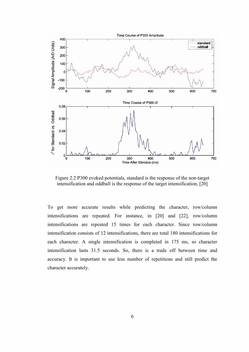
Figure 2.2 P300 evoked potentials, standard is the response of the non-target

intensification and oddball is the response of the target intensification, [20] ....... 6

Figure 3.1 Principal components (drawn with red lines) for data set that sampled

from noisy y = x line is given in (a). PCA transformation for data is given in (b).

............................................................................................................................. 13

Figure 3.2 Lines (1 dimensional hyperplane) that are separating two classes in two

dimensional space................................................................................................ 17

Figure 3.3 SVM solution for maximum-margin line (1 dimensional hyperplane)

separating two classes for the data set given in Figure 3.2 ................................. 18

Figure 3.4 SVM solution for soft margin line (1 dimensional hyperplane) for C=100

............................................................................................................................. 21

Figure 3.5 Classification and Regression Tree example, xi is the i'th dimension

value of x and y is the class label ........................................................................ 25

Figure 4.1 Randomly selected target and non-target intensifications extracted 0-800

ms after stimulus ................................................................................................. 28

Figure 4.2 Averaged target and non-target intensifications for train and test data set

extracted 0-800 ms after stimulus, channels 1-16 ............................................... 30


extracted 0-800 ms after stimulus, channels 17-32 ............................................. 31



xiv



Figure 4.6 8th order bandpass Chebyshev Type I filter with cut-off frequencies 0.1

Hz and 10 Hz....................................................................................................... 35

Figure 4.7 Effect of filtering with 8th order 0.1 – 10 Hz bandpass Chebyshev Type-I

filter on a target intensification ........................................................................... 36

Figure 4.8 Effect of filtering with 8th order 0.1 – 10 Hz bandpass Chebyshev Type-I

filter on a non-target intensification .................................................................... 37

Figure 4.9 Average time domain feature vectors of target (oddball) and non-target

(standard) classes for channel 11......................................................................... 39

Figure 4.10 Average time domain simple normalized (mapped to [-1, 1]) feature

vectors of target (oddball) and non-target (standard) classes for channel 11...... 40

Figure 4.11 Average time domain Gaussian normalized feature vectors of target

(oddball) and non-target (standard) classes for channel 11................................. 41


(standard) classes obtained by the absolute value of the signals for channel 11. 42


(standard) classes obtained by the normalized energy distribution of the signals

for channel 11...................................................................................................... 43


(standard) classes obtained by the normalized energy distribution of the signals

with offset trick for channel 11 ........................................................................... 44


(standard) classes obtained by the sum of all frequency components in WVD for

channel 11............................................................................................................ 45

Figure 4.16 Average time-frequency domain feature vectors of target (oddball) and

non-target (standard) classes obtained from the WVD for channel 11. .............. 47

Figure 4.17 Correlation coefficients between channel 11 and other 64 channels.... 48

Figure 4.18 Average feature vectors of target (oddball) and non-target (standard)

classes for channels 3, 4, 5, 10, 11, 12, 17, 18, 19 .............................................. 50

Figure 4.19 Average PCA transformed feature vectors of target (oddball) and non-

target (standard) classes for channels 3, 4, 5, 10, 11, 12, 17, 18, 19................... 51

xv

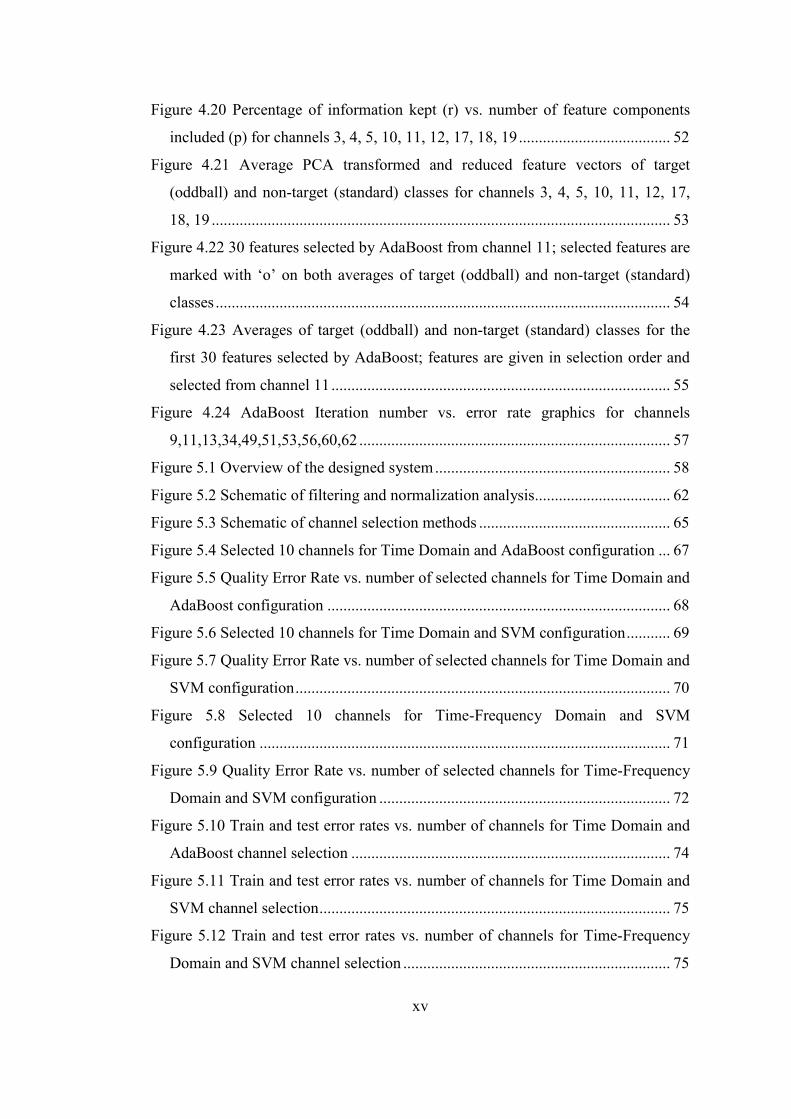
Figure 4.20 Percentage of information kept (r) vs. number of feature components

included (p) for channels 3, 4, 5, 10, 11, 12, 17, 18, 19...................................... 52

Figure 4.21 Average PCA transformed and reduced feature vectors of target

(oddball) and non-target (standard) classes for channels 3, 4, 5, 10, 11, 12, 17,

18, 19 ................................................................................................................... 53

Figure 4.22 30 features selected by AdaBoost from channel 11; selected features are

marked with ‘o’ on both averages of target (oddball) and non-target (standard)

classes .................................................................................................................. 54

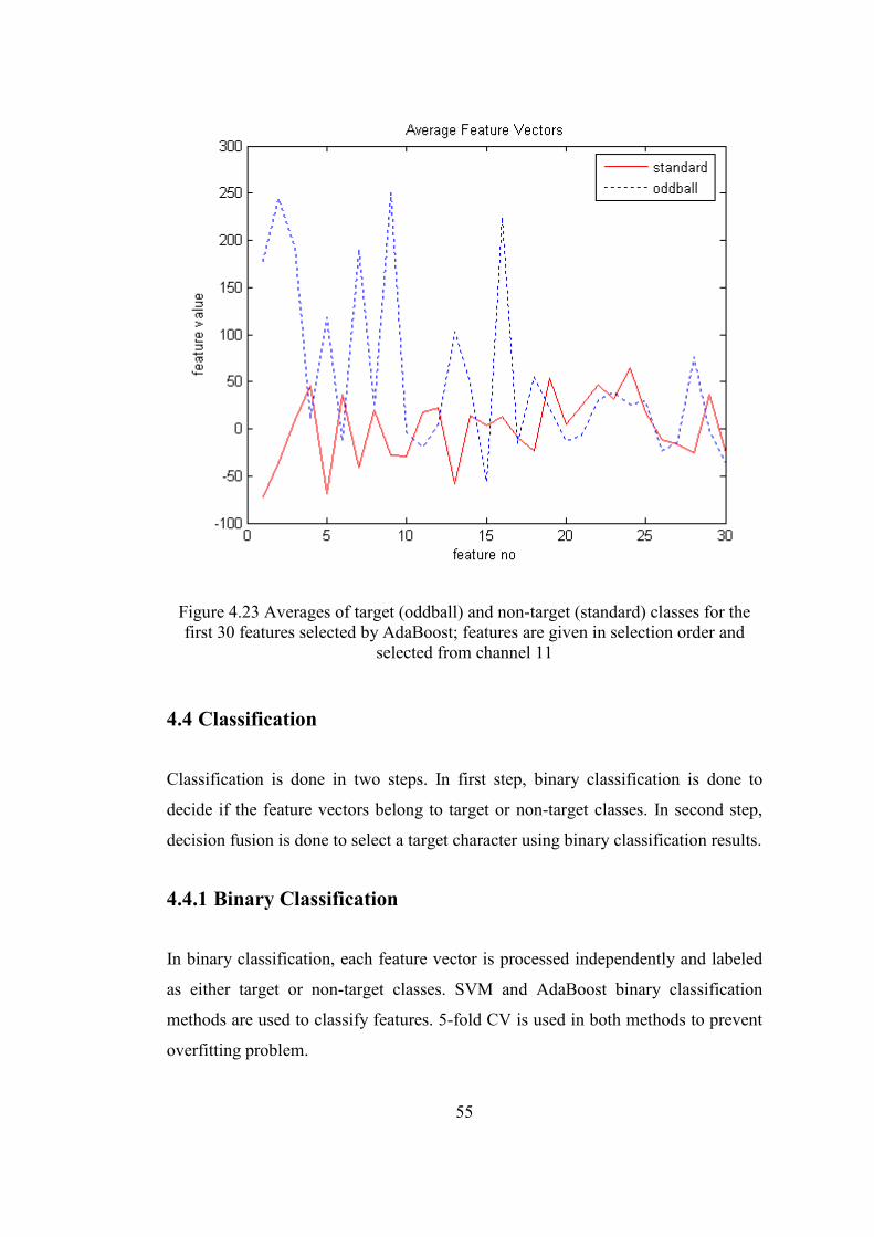
Figure 4.23 Averages of target (oddball) and non-target (standard) classes for the

first 30 features selected by AdaBoost; features are given in selection order and

selected from channel 11..................................................................................... 55

Figure 4.24 AdaBoost Iteration number vs. error rate graphics for channels

9,11,13,34,49,51,53,56,60,62 .............................................................................. 57

Figure 5.1 Overview of the designed system........................................................... 58

Figure 5.2 Schematic of filtering and normalization analysis.................................. 62

Figure 5.3 Schematic of channel selection methods ................................................ 65

Figure 5.4 Selected 10 channels for Time Domain and AdaBoost configuration ... 67

Figure 5.5 Quality Error Rate vs. number of selected channels for Time Domain and

AdaBoost configuration ...................................................................................... 68

Figure 5.6 Selected 10 channels for Time Domain and SVM configuration........... 69

Figure 5.7 Quality Error Rate vs. number of selected channels for Time Domain and

SVM configuration.............................................................................................. 70

Figure 5.8 Selected 10 channels for Time-Frequency Domain and SVM

configuration ....................................................................................................... 71

Figure 5.9 Quality Error Rate vs. number of selected channels for Time-Frequency

Domain and SVM configuration ......................................................................... 72

Figure 5.10 Train and test error rates vs. number of channels for Time Domain and

AdaBoost channel selection ................................................................................ 74

Figure 5.11 Train and test error rates vs. number of channels for Time Domain and

SVM channel selection........................................................................................ 75

Figure 5.12 Train and test error rates vs. number of channels for Time-Frequency

Domain and SVM channel selection ................................................................... 75

xvi

Figure 5.13 12 channels selected by Time Domain and SVM channel selection

method ................................................................................................................. 78

Figure 5.14 Schematic of dimensionality reduction methods.................................. 79

Figure 5.15 Percentage of information kept (r) vs. number of feature components

included (p) for selected 12 channels .................................................................. 80

Figure 5.16 PCA dimension reduction results ......................................................... 81

Figure 5.17 AdaBoost dimension reduction results ................................................. 82

Figure 5.18 Performance vs. repetition number results for reference channels on 42

character train set................................................................................................. 84

Figure 5.19 Performance vs. repetition number results for selected 12 channels on

42 character train set............................................................................................ 84

Figure 5.20 Performance vs. repetition number results for reference channels on 31

character test set .................................................................................................. 85

Figure 5.21 Performance vs. repetition number results for selected 12 channels on

31 character test set ............................................................................................. 86

1

CHAPTER 1

INTRODUCTION

Human being performs all voluntary movements by controlling related organs with

the brain. Diseases may cause partial or full loss of abilities of the patients. In

diseases such as Amyotrophic Lateral Sclerosis (ALS), all voluntary movements of

the patient can be disabled and only cognitive abilities of the brain remain

unaffected. So, these patients can interact with outside world only using their brain

signals. Brain Computer Interface (BCI) is an area of research that tries to increase

the interaction of such patients with outside world by processing activities of the

brain and controlling external devices. For example, a cursor was moved in a two-

dimensional maze by human using signals recorded via Electroencephalography

(EEG) in 1977 [1]. With the improvements in technology, studies on BCI are

increased and research groups are founded over past decades. Researchers try the

increase the applications of BCI and increase the usability of the systems developed

([6]-[11]).

There are two types of BCI’s according to their input types. These input types are

endogenous and exogenous electrophysiological activities. In endogenous BCI’s,

the subject creates control signals by imagination without any external stimulus.

One of main methods to create these signals is imagination of muscle movement

([2], [3]) such as imagining right and left hand movements. Another method is

thinking abstract feelings ([4], [5]) such as stress and relaxation. In exogenous

BCI’s, the subject creates control signals evoked by an external stimulus. For

instance, the method developed in [17] is allowing subjects to communicate letters

2

and words using Event-Related Potentials (ERP’s). Endogenous BCI’s require

excessive training while learning creation of control signals. However, once it is

learned, subject can create signals on its own. On the other hand, exogenous BCI’s

does not require too much training but it needs an external stimulus such as a

display to create control signals.

A laboratory environment is needed to gather data and work on BCI. Fortunately, in

recent years, BCI research groups started to organize competitions and provide data

sets to the competitors ([12]-[15]). These competitions aim to improve the BCI

development process by introducing challenging problems and creating

environment to compare different methods. Competition datasets are still available

and can be accessed through the webpage given in [12]. So, new approaches can be

tried on the same data set and results can be compared with previous studies.

In this thesis, Spelling Paradigm, a specific exogenous BCI application, is studied.

Spelling Paradigm was first introduced by Donchin et al. [17] in 1988. In 2000, a

new version of Spelling Paradigm with increased data transformation rate was

introduced by Donchin et al. [18]. Spelling Paradigm is an application for disabled

people to express their thoughts by constructing words from detected letters.

Spelling Paradigm problems exist in BCI competitions [14] and [15]. Data set is

also available on [20] and [22]. In this thesis, time domain and time-frequency

domain responses of P300 evoked potentials of Spelling Paradigm data set are

analyzed. Time domain signals are transformed into time-frequency domain using

Wigner-Ville Distribution (WVD). EEG signals are recorded using several

electrodes attached to the scalp. Optimum electrode subset among the recorded ones

is searched. Working on small data sets increases the speed of the process and real

time use of the system. Effect of feature reduction methods Principal Component

Analysis (PCA) and AdaBoost on feature vectors is analyzed. Support Vector

Machine (SVM) and AdaBoost are used for classification throughout the process.

3

Organization of the thesis is given as:

In Chapter 2, introductory information about Spelling Paradigm is given and

previous studies on this problem are analyzed.

In Chapter 3, background information about filtering, normalization, feature

transformation, dimension reduction and classification methods are given.

In Chapter 4, details of implemented methods are given.

In Chapter 5, experimental results about feature transformation methods, optimum

channel selection results, effect of dimension reduction and classification methods

are given.

In Chapter 6, results are discussed and thesis is concluded.

4

CHAPTER 2

SPELLING PARADIGM

Spelling Paradigm is a BCI application which aims to detect the words by finding

letters from brain activities of the person. It is introduced by Farewell and Donchin

[17]. In this chapter, first, Spelling Paradigm experimental setup and data set is

described in detail. Then, previous studies on this topic are summarized. Finally,

implemented methodologies are discussed.

2.1 Spelling Paradigm Definition

The goal of the spelling paradigm is to give an interface to construct words by using

only the electrical activity of the brain. 6 by 6 matrix which is composed of ASCII

characters is displayed on a screen (Figure 2.1). Subject is requested to focus on a

character in the matrix. Then, rows and columns of the matrix are successively and

randomly intensified. There are total 12 rows and columns and only 2 of them

contain the focused character. From now on, rows and column intensifications that

contain desired character will be named as target intensifications and rows and

column intensifications that do not contain desired character will be named as non-

target intensifications.

5

Figure 2.1 Spelling Paradigm character matrix that is displayed to user is given in (a) and row and column number assignments of the matrix is given in (b), [20]

Response of the brain against target and non-target intensifications is different and

their responses are similar to the P300 evoked potentials reported by Farewell and

Donchin [17]. The P300 evoked potential is the reaction of the subject to the

stimulus. Its occurrence is not related with the physical attributes of a stimulus. It is

a positive deflection in voltage with latency (delay between stimulus and response)

of roughly 300 to 600 milliseconds. In spelling paradigm, P300 evoked potentials

are elicited using the Oddball Paradigm [23]. The oddball paradigm is a technique

used in evoked potential research in which trains of stimuli that are usually auditory

or visual are used to assess the neural reactions to unpredictable but recognizable

events. In this case, low-probability target intensifications are inter-mixed with

high-probability non-target (or "standard") intensifications. The subject’s reaction to

the target intensifications elicits the P300 evoked potentials (Figure 2.2).

(a) (b)

6

Figure 2.2 P300 evoked potentials, standard is the response of the non-target intensification and oddball is the response of the target intensification, [20]

To get more accurate results while predicting the character, row/column

intensifications are repeated. For instance, in [20] and [22], row/column

intensifications are repeated 15 times for each character. Since row/column

intensification consists of 12 intensifications, there are total 180 intensifications for

each character. A single intensification is completed in 175 ms, so character

intensification lasts 31.5 seconds. So, there is a trade off between time and

accuracy. It is important to use less number of repetitions and still predict the

character accurately.

7

2.2 Spelling Paradigm Solution Approach

Spelling paradigm is separated into three main steps. These steps are extracting

samples, creating features and classifying features.

First step is extracting relevant information from recorded EEG signals. EEG

signals consist of multiple channel data which are recorded using electrodes placed

on different points of the skull. Using less number of channels reduces the

computational effort. However, relevant information must be kept by selecting

proper set of channels. Part of the EEG signal that contains relevant information

must be extracted. P300 evoked potential characteristics are taken into account

while determining the duration of the signal after the stimulus. Then, extracted

signals can also be filtered to suppress noise.

Second step is extracting features from the preprocessed signals which are the

output of the first step. Time domain signals can be transformed into other domains

and transformed channels are concatenated to create features. Then, features can be

normalized and size of the features can be reduced.

Final step is the classification of the features. First, each intensification is classified

separately and then character decision is done using the repetitions.

2.3 Previous Studies on Spelling Paradigm

Studies on spelling paradigm are encouraged by competitions [20] and [22]. Data

set is provided by the organizers of results are evaluated. By this way, effect of

different algorithms can tested on same data and results can be compared.

7 competitors attended to the competition [20] and 5 of them managed to classify all

the words correctly using all 15 repetitions. Other than success rate, using less

number of repetitions is also an evaluation criterion of the performance. All words

are correctly classified using only 5 repetitions by Kaper [24].

8

10 competitors attended to the competition [22], and Rakotomamonjy [30] won the

competition by achieving %96.5 accuracy with 15 repetitions and %73.5 accuracy

with 5 repetitions.

Studies are continued after the completion of the competition. For instance,

Erdoğan successfully implemented Wiener filter in his thesis study and gave the

results in [29].

Previous solution attempts on Spelling Paradigm are evaluated in terms of their

methods on three main steps, preprocessing signals, extracting features and

classifying features.

2.3.1 Preporcessing Signals

In preprocessing step, a channel subset is decided and a signal portion is extracted

from these channel sets after intensification. Filtering and downsampling are other

methods applied at this step.

Kaper [24], used 10 channels in his study, used a bandpass filter with cutoff

frequencies (0.5 – 30) and extracted signals of interval 0-600 ms after stimulus.

Erdoğan [29] used same channel subset and the same time interval after stimulus

with [24]. But he applied the adaptive Wiener filter instead of standard filters.

Rakotomamonjy [30] did not use fixed channels. Instead, channels are selected

automatically among the whole channel set with elimination. So, an adaptive

channel selection method is applied. Then signals are filtered with (0.1 – 10 Hz)

bandpass filter and downsampled to 20 Hz. 0-667 ms signals are extracted after

stimulus. Bostanov [25] used all channels, a 10 Hz lowpass filter and a logarithmic

downscaling. One second interval after stimulus is extracted. Xu [26] used all

channels, 2-8 Hz bandpass filter and 0-650 ms interval. Hoffmann [32] used the

same 10 channels given in [24]. 0-9 Hz filter, 0-600 ms time interval after stimulus

and downsampling is used. Yang [31] used 55 channels selected with F-score, 0.1 –

20 Hz bandpas filter, 0-667 ms time interval after stimulus and downsampled

9

signals to 20 Hz. Rivet [33] used 1-20 Hz bandpass filter with 1 second interval

after stimulus.

2.3.2 Feature Extraction

Preprocessed signals are transformed into feature spaces and used channels are

concatenated to create feature vectors. Dimension of the feature vectors are also

reduced in this step.

Kaper [24], Erdoğan [29], Rakotomamonjy [30], Yang [31], Hoffmann [32],

concatenated preprocessed signals without transforming or reducing its size.

Bostanov [25] transformed signals using Continuous Wavelet Transform and

Student’s two-sample t statistics. Xu [26] used Principal Component Analysis

(PCA) and Independent Component Analysis (ICA) for both transforming signals

into feature space and reducing dimension. Rivet [33] used xDAWN algorithm, a

spatial filter, to transform signals.

2.3.3 Classification

Feature vectors are classified with learning methods at final step.

Kaper [24], Erdoğan [29], Rakotomamonjy [30], Yang [31], used SVM in their

studies. Hoffmann [32] used gradient boosting, Bostanov [25] used Linear

Discriminant Analysis (LDA), and Rivet [33] used Bayesian LDA for classification.

2.4 Conclusion

Although the classification methods in most of the previous studies are similar to

each other, performances of the systems are different. So, pre-processing and

feature extraction steps distinguish the performance of the systems. Filtering, is

generally applied to enhance the performance of the system. Downsampling is also

preferred after filtering. Channel selection varies significantly between methods.

Methods can use all channels and then reduces data size at feature extraction or

10

select a subset of channels and create already reduced number of features at the end

of preprocessing step. Time domain is generally preferred for P300 analysis.

11

CHAPTER 3

BACKGROUND

3.1 Wigner-Ville Distribution

Wigner-Ville Distribution (WVD) transforms time signals into time-frequency

domain. WWD of a signal s(t) is given in equation (3-1).

ττπττ dfj

etstsftW2

)2/(*)2/(),(−−

∞+

∞−

+= ∫ (3-1)

WWD satisfies the marginal conditions given in equations (3-2) and (3-3) for the

signal s(t), defined for t between 0 and t1 and f between 0 and f1.

)(

0

),(1

fESD

t

dtftW =∫ (3-2)

21

)(

0

),( ts

f

dfftW =∫ (3-3)

where ESD(f) is the energy spectral density of the signal (the intensity of energy per

unit frequency), and 2

)(ts is the signal power at time t.

12

For a time-series x(n), the expression of the discrete-time Wigner-Ville distribution,

W(n,f) is:

∑∞

−∞=

−−+=k

kfjeknxknxkhfnW N

π4)(*)()(22),( (3-4)

where )(khN is a data-window, which performs a frequency smoothing.

3.2 Principal Component Analysis

Principal Component Analysis (PCA) is an orthogonal linear transformation method

that transforms the data to a new basis according to variance of the data. The axes

of the new coordinate system (principal components) are ordered with decreasing

variance. That is, the greatest variance direction is the first axis (first principal

component) and smallest variance direction is the last axis. PCA is commonly used

for reducing dimensionality of the data set. Possibly correlated variables are also

eliminated while projecting data to the lower dimensional space.

PCA Example:

In Figure 3.1, data is sampled from noisy y = x line is plotted. Principal components

for the data set are also plotted.

13

Figure 3.1 Principal components (drawn with red lines) for data set that sampled from noisy y = x line is given in (a). PCA transformation for data is given in (b).

(b)

(a)

14

Table 3.1 Principal components’ eigenvectors and eigenvalues for the data set given in Figure 3.1

Principal Component 1 Principal Component 2

Eigenvector [0.7002 0.7139] [-0.7139 0.7002]

Eivenvalue 18.2577 0.2394

Assumptions and Limitations of PCA:

• PCA is based on mean vector and covariance matrix of the data. If

distribution of the data can not be characterized by these attributes, PCA is not

useful.

• Principal components with larger variance contain more information about

data set.

• Principal components are selected as orthogonal to reduce the computational

complexity. So, it only rotates the coordinate system.

3.3 Normalization

Normalization is a standardization of collected data in order to recover errors of the

repeated measurements. Variety of normalization methods exist, which are using

the properties of each sample or statistical properties of the whole data set.

Collected samples are assumed to be in vector form.

Scaling magnitude, which is called as simple normalization, is one of the most

common and easy normalization methods. In simple normalization, properties of a

single vector are sufficient to apply normalization. Minimum and maximum

magnitude values of the vector are used while normalizing the vector. Using these

properties, vector is scaled to the predefined range.

15

For a vector x , where maximum value of x is )max(x and minimum value of x

is )min(x , formula that maps x into the region [ )max(),min( xx ] is given in (3-5).

)min())min(()min()max(

)min()max(xxx

xx

xxx +−×

−−

= (3-5)

Scaling mean and standard deviation of the signals, which is called Gaussian

normalization, is another normalization method. Mean and standard deviation are

statistical properties of data set. So, whole data set is required to calculate these

properties. Mean is normalized to zero and standard deviation is normalized to unity

at Gaussian normalization.

Gaussian normalization formula is given in equation (3-6) for the vector x , where

xµ and xσ are mean and standard deviation respectively.

x

xxx

σµ−

= (3-6)

3.4 Kernel Methods

Kernel Methods (KMs) map the data into a higher dimensional space. This space is

called feature space and each coordinate of the feature space corresponds to a

feature of the data. Non-linear models in the input space can be solved by linear

models in the feature space. Transformation from the input space to the feature

space is done by the help of kernel functions. Kernel functions enable to operate in

the feature space without even computing the coordinates of the data in that space.

Instead, inner products between the images of all pairs of data are computed in the

feature space, which is generally less complex than the explicit computation of the

coordinates. Various methods such as SVM, Fisher’s Linear Discriminant Analysis

(LDA) and Principal Component Analysis (PCA) are capable of operating with

kernels.

16

A kernel function K is non-negative, real valued and integrable. Kernel function

satisfies the following the requirements:

• ∫+∞

∞−

= 1)( duuK

(3-7)

• u of valuesallfor )()( uKuK =− (3-8)

Examples of kernel functions:

Linear Kernel:

yxyxK .),( = (3-9)

Polynomial Kernel:

Control parameter is polynomial degree d.

( )dyxyxK 1.),( += (3-10)

Radial Basis Function:

−−=

2

2

2exp),(

σ

yxyxK

(3-11)

Exponential Kernel:

−−=

22exp),(

σ

yxyxK

(3-12)

3.5 Support Vector Machine

Support Vector Machine (SVM), which is introduced by Vapnik in 1963, is a

supervised learning method, which analyzes the input-output relation of the training

data to predict the outputs for the new input data. When the outputs are discrete,

17

prediction is called classification of the input data. SVM is a linear classifier, which

uses hyperplane to separate data into classes. SVM is originally applied to two class

classification problems. There are various solutions to separate linearly separable

two classes given in Figure 3.2. SVM is aimed to find the maximum margin

hyperplane while separating data into two classes (see Figure 3.3).

Figure 3.2 Lines (1 dimensional hyperplane) that are separating two classes in two dimensional space

18

Figure 3.3 SVM solution for maximum-margin line (1 dimensional hyperplane) separating two classes for the data set given in Figure 3.2

Suppose that data set consists of p-dimensional n samples x belonging to linearly

separable two classes c. The aim is to find the p-1 dimensional hyperplane which

separates the classes with maximum margin. Labels }1,1{ −=c will be used for two

classes. Mathematical form of a hyperplane is

,0=−⋅ bxw (3-13)

where w is the normal vector and b is the bias vector. Hyperplanes passing through

the margins of the classes can be chosen as

1±=−⋅ bxw (3-14)

Since samples belonging to two classes have to be the outside of the hyperplanes

defining the margin,

19

,1≥−⋅ bxw i (3-15)

where xi belongs to class labeled with {1} and

,1−≤−⋅ bxw i (3-16)

where xi belongs to class labeled with {-1}.

( ) nibxwc ii ≤≤≥−⋅ 1 allfor ,1 (3-17)

The aim is to maximize the margin between two classes. The distance between two

hyperplanes given in (3-14) isw

2. So, minimizing w , the norm of w, will

maximize the distance between two classes. Using the quadratic programming

2

2

1w will be minimized while satisfying (3-17).

The optimization problem can be constructed with the Lagrange multipliers

technique:

( )[ ],12

1),,(

1

2−+⋅−=Λ ∑

=

bxwcwbwL ii

n

i

iλ (3-18)

where },...,{ 1 nλλ=Λ is the vector of non-negative Lagrange multipliers

corresponds to the constraints in (3-17). The Lagrangian given in (3-18) is

minimized with respect to w and b and maximized with respect to 0≥Λ .

The solution of the problem can be expressed as a linear combination of training

vectors:

ii

n

i

i xcw ∑=

=1

λ (3-19)

So, maximum margin hyperplane is found by solving the optimization problem

given in the Lagrangian dual form:

20

n1,...,ifor 0

0 subject to

2

1)( Maximize

1

1 11

=≥

=

⋅−=Λ

∑

∑∑∑

=

= ==

i

n

i

ii

n

i

n

j

jijiji

n

i

i

c

xxccL

λ

λ

λλλ

(3-20)

The training vectors that have coefficients satisfying 0>λ are called support

vectors. Support vectors satisfy the equation 1)( =−⋅ bxwc ii . So, b can be

calculated using any support vector.

Decision function becomes:

( )

+⋅= ∑

=

bxxcsignxf ii

n

i

i

1

)( λ (3-21)

Soft Margin Hyperplane

Train vectors can not be separated by a hyperplane due to mislabeled data in Figure

3.4. SVM is modified [27] to handle linearly inseparable classes by introducing Soft

Margin method.

21

Figure 3.4 SVM solution for soft margin line (1 dimensional hyperplane) for C=100

Soft Margin method introduces slack variables iξ that measure the amount of

violation of the constraints. A penalty coefficient is added to the optimization

problem with regularization parameter C:

( )n1,...,ifor ,0

,...,1ifor ,1 subject to

2

1 Minimize

i

1

2

=≥

=−≥−⋅

+ ∑=

ξ

ξ

ξ

nbxwc

Cw

iii

n

i

i

(3-22)

The modified optimization problem can be constructed with the Lagrange

multipliers technique:

( )[ ] ,12

1),,,,(

111

2 ∑∑∑===

+−+−+⋅−=ΓΞΛn

i

i

n

i

iiiii

n

i

i CbxwcwbwL ξξγξλ (3-23)

22

where },...,{ 1 nλλ=Λ and },...,{ 1 nγγ=Γ are the vector of non-negative Lagrange

multipliers corresponds to the constraints in (3-22). The Lagrangian given in (3-23)

is minimized with respect to w, Ξ and b and maximized with respect

to 0≥Λ and 0≥Γ .

Maximum margin hyperplane is found by solving the optimization problem given in

the Lagrangian dual form:

n1,...,ifor 0C

0 subject to

2

1)( Maximize

1

1 11

=≥≥

=

⋅−=Λ

∑

∑∑∑

=

= ==

i

n

i

ii

n

i

n

j

jijiji

n

i

i

c

xxccL

λ

λ

λλλ

(3-24)


( )

+⋅= ∑

=

bxxcsignxf ii

n

i

i

1

)( λ (3-25)

where bias b is calculated from the equation:

( )[ ] nbxwc iii ,...,1ifor 0 1 i ==+−−⋅ ξλ (3-26)

There are constraints in the equation (3-26) coming from (3-22) that limits the value

of the λi to C<< i0 λ . 0 i >λ is valid for only the support vectors. C<i λ is valid

for only correctly classified vectors. So, only correctly classified support vectors

can be used for calculation of bias b. Note that there can be multiple solutions for b.

Common approach is to solve all equations and then take the averages of the results:

, 1

1i

N

i

i

SV

cxwN

bSV

∑=

−⋅= (3-27)

where xi are correctly classified support vectors and NSV is the number of xi.

23

Non-Linear Decision Surfaces

As it is stated in KMs, SVM are also used for classifying non-linear data set by

transforming it into higher dimensional feature space where data can become

linearly separable. In (3-25), decision function depends on dot product of vectors

which defines hyperplanes for decision boundaries. If the dot product is changed

with a kernel function, non-linear decision surfaces are obtained for decision

boundaries. This is called kernel trick.


( )

+⋅= ∑

=

bxxKcsignxf ii

n

i

i

1

)( λ (3-28)

3.6 AdaBoost

AdaBoost is an adaptive boosting algorithm which is introduced in 1995 by Freund

and Schapire [28]. AdaBoost constructs a strong classifier as a linear combination

of weak classifiers.

Suppose that train set consists of m elements ( ) ( ) }1,1{,;,...,11 +−∈∈ iimm yXxyxyx .

Then, pseudo code of the AdaBoost algorithm is:

Initialize

miD 1)(1 = (3-29)

For Tt ,...,1=

• Train weak classifier using the distribution Dt

• Get weak hypothesis }1,1{: +−→Xht with error

( )[ ] ( )∑≠

=≠=

iit

tiitt

Dit

yxhi

iDyxh

:

Pr ~ε (3-30)

24

• Choose

−=

t

t

t εε

α1

ln2

1 (3-31)

• Update:

( ) ( ) ( )( )

( ) ( )( )t

ititt

iitt

iitt

t

tt

Z

xhyiD

yxhe

yxhe

Z

iDiD

α

α

α

−=

≠

=×=

−

+

exp

if

if 1

(3-32)

where Zt is a normalization factor (chosen so that Dt+1 will be a distribution).

• Output the final hypothesis:

∑=

=T

t

tt xhxH1

)()( α (3-33)

In (3-31), αt is inversely proportional with εt. That is, having a larger αt coefficient

means that the corresponding weak hypothesis classifies more accurately. The

distribution Dt(i) is updated such that weight of the correctly classified samples are

decreased and weight of the misclassified samples are decreased in the next cycle.

By this way, algorithm focuses on the misclassified samples in next cycles.

3.6.1 Classification and Regression Trees

Classification and Regression Trees (CART) is used as the weak classifier of the

AdaBoost. Decision tree consists of nodes and leaves. Tree is tracked from root to

leaves to find out the class of the corresponding input.

Suppose that x is an n dimensional input, where xi is the value of the i’th dimension

of x, and y is the binary classification output which is an element of {-1, +1}. Then,

leaf of the tree contains the predicted class label y and node of the tree contains the

relational condition which compares xi with a threshold value. Decision tree is

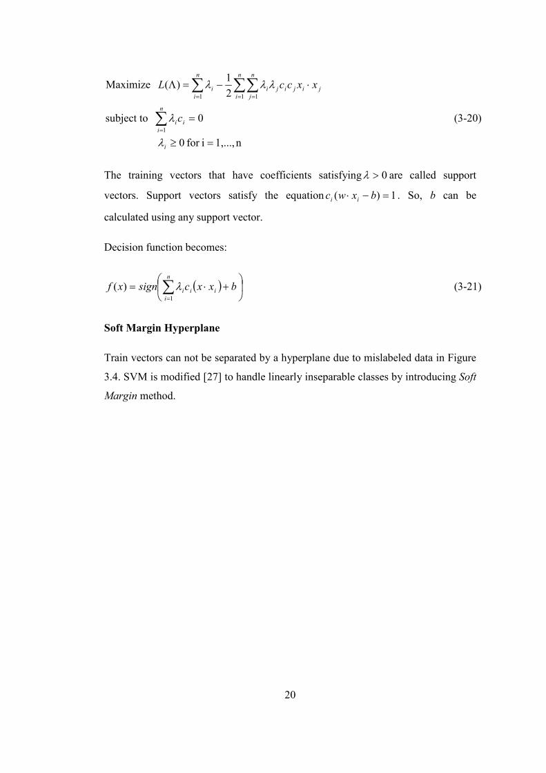
25

constructed at training phase by choosing the dimension variable i and threshold

value of the node and class label of the leaf. A sample CART is given in Figure 3.5.

Figure 3.5 Classification and Regression Tree example, xi is the i'th dimension value of x and y is the class label

3.7 Cross Validation

In predictive models, if the validation set used for testing the parameters of the

model is selected from the training set, model parameters may become quite

dependant on the training data. Thus, model’s prediction performance on unseen

data may not be as satisfactory as if it is on the train data. This is called overfitting

problem. To overcome this problem, cross-validation is used. Cross-validation is a

method to evaluate the accuracy of the predictive model. Train set is divided into

two subsets. One subset is used for training and the other subset is used for

validating the model. It prevents overfitting problem since training and validation

data sets are constructed from different subsets of the training set.

26

In k-fold cross-validation, training data is divided into k partitions and k-1 partitions

are used for training and 1 partition is used for testing the model. This cross-

validation process is repeated k times such that at each round, another partition is

used for testing the model. While creating partitions, data can be also stratified to

have a better representation of the whole data. Stratification ensures that samples of

each class are equally distributed into each fold. That is, each fold is composed of

equally sized members of the whole classes.

27

CHAPTER 4

IMPLEMENTATION

EEG signals are processed in three steps. First, relevant part of the signal is

extracted from data. Then, signals are transformed into feature space and dimension

of the feature vector is reduced. Finally, classification is performed using the

extracted features. Spelling Paradigm data set provided in [20] is used to test the

proposed methods.

4.1 Preprocessing EEG Signals

The whole activity of the brain is recorded by the electrodes while collecting data

during the intensifications. However, only the part related with the stimulus is

needed for processing. To remove irrelevant information, collected data is

preprocessed. Preprocessing consists of three steps. First one is selecting signal

portion related with stimulus and second one is filtering the selected portion of the

signal to suppress noise and third one is downsampling data.

4.1.1 Extracting Data

EEG signals for 64 channels, row/column number (or stimulus code),

intensification’s start time are available in data set provided in [20]. Besides,

character labels for train data set are also given. Since competition is over, test

labels of the data set are also available. To increase the flexibility of the analysis,

channel subset, signal duration, and number of repetitions are made configurable in

28

the system. By this way, different setups are easily established. Stimulus code is

used for separating rows and columns in next steps. Number of repetitions used is

also adjustable to analyze the prediction results for less number of repetitions.

For each target intensification, there are 5 non-target intensifications in train data

set. Number of target and non-target intensifications need to be equalized to obtain

a well-balanced train data set. For each target row and column, a non-target row and

column is selected randomly. A sample for a single target and non-target

intensifications are given in Figure 4.1.

Figure 4.1 Randomly selected target and non-target intensifications extracted 0-800 ms after stimulus

Target and non-target intensifications for train and test data set is extracted for 800

ms duration after the stimulus and averaged plots are given in Figure 4.2, Figure

29

4.3, Figure 4.4, and Figure 4.5 for channels 1-16, 17-32, 33-48 and 49-64

respectively.

30

Figure 4.2 Averaged target and non-target intensifications for train and test data set extracted 0-800 ms after stimulus, channels 1-16

Fig

ure

4.2

Ave

rage

d ta

rget

and

non

-tar

get

inte

nsif

icat

ions

for

tra

in a

nd t

est

data

set

ext

ract

ed 0

-800

ms

afte

r st

imul

us,

chan

nels

1-1

6

31


Fig

ure

4.3

Ave

rage

d ta

rget

and

non

-tar

get

inte

nsif

icat

ions

for

tra

in a

nd t

est

data

set

ext

ract

ed 0

-800

ms

afte

r st

imul

us,

chan

nels

17-

32

32


Fig

ure

4.4

Ave

rage

d ta

rget

and

non

-tar

get

inte

nsif

icat

ions

for

tra

in a

nd t

est

data

set

ext

ract

ed 0

-800

ms

afte

r st

imul

us,

chan

nels

33-

48

33


Fig

ure

4.5

Ave

rage

d ta

rget

and

non

-tar

get

inte

nsif

icat

ions

for

tra

in a

nd t

est

data

set

ext

ract

ed 0

-800

ms

afte

r st

imul

us,

chan

nels

49-

64

34

P300 evoked potentials are observed approximately 300 ms after the stimulus. It is

seen from 4 figures, Figure 4.2, Figure 4.3, Figure 4.4, and Figure 4.5, that

extracting signals [100-600] ms after stimulus keeps all of the information related

with P300 evoked potentials.

4.1.2 Filtering

When 4 figures, Figure 4.2, Figure 4.3, Figure 4.4, and Figure 4.5, are investigated,

it is seen that P300 evoked potentials contain the information in low frequency

components. Since signals are sampled at 240 Hz, high frequency components are

filtered to reduce the effect of noise. Characteristics of 8th order Chebyshev Type-I

bandpass filter with cut-off frequencies 0.1-10 Hz is given in Figure 4.6. This filter

was used by Rakotomamonjy at al. [30].

35

Figure 4.6 8th order bandpass Chebyshev Type I filter with cut-off frequencies 0.1 Hz and 10 Hz

Effect of the filtering with Chebyshev Type-I filter given in Figure 4.6 on the target

and non-target signals of Figure 4.1 are given in Figure 4.7 and Figure 4.8

respectively.

36

Figure 4.7 Effect of filtering with 8th order 0.1 – 10 Hz bandpass Chebyshev Type-I filter on a target intensification

37

Figure 4.8 Effect of filtering with 8th order 0.1 – 10 Hz bandpass Chebyshev Type-I filter on a non-target intensification

4.1.3 Downsampling

Downsampling is the last method that is applied in the preprocessing step. Signals

are generally sampled at frequencies higher than the interest. Filtering suppresses

frequency components that are out of interest. However, it does not change the

sampling rate. Since signals sampled at high frequency rates are filtered, sampling

rate of the signal can be reduced by representing a group of samples with a single

sample. By this way, size of the signal is also reduced and thus process speed of the

next steps is increased. Downsampling is done by averaging samples with non-

overlapping windows. That is, signal is partitioned into pieces and each piece is

represented with the average of samples in it. Length of each piece is determined by

the window length parameter. New sampling frequency becomes original sampling

frequency divided by the window length. Window length is adjustable and if it is

38

selected to be 1, downsampling is skipped. When the window length is greater than

1, high frequency noise components are also suppressed with averaging consecutive

samples in addition to dimension reduction.

4.2 Feature Extraction

Feature vectors are extracted after relevant part of the recorded brain signals are

extracted from data. While extracting feature vectors, each channel is transformed

into the feature space and then all channels are concatenated. Time and time-

frequency domains are used as feature spaces in this study. Feature vectors are

normalized with simple or Gaussian normalization methods to minimize the effect

of time varying offset and amplitude of the signal. That is, dependency on sampling

time and subject is reduced by normalizing features. Samples are extracted from

time interval [100-600] ms after stimulus unless otherwise it is stated.

4.2.1 Time Domain Features

No transformation is done in time domain. Channel outputs are directly

concatenated to obtain feature vectors. Average feature vectors extracted without

filtering and normalization for a single channel are given in Figure 4.9.

39

Figure 4.9 Average time domain feature vectors of target (oddball) and non-target (standard) classes for channel 11

Simple normalization and Gaussian normalization methods are applied to channel

11 data and results are given in Figure 4.10 and Figure 4.11 respectively.

40

Figure 4.10 Average time domain simple normalized (mapped to [-1, 1]) feature vectors of target (oddball) and non-target (standard) classes for channel 11

41

Figure 4.11 Average time domain Gaussian normalized feature vectors of target (oddball) and non-target (standard) classes for channel 11

4.2.2 Time-Frequency Domain Features

Wigner-Ville Distribution (WVD) is used to create time-frequency features of the

system. Before starting the analysis in time-frequency domain, energy of the signal

is investigated. Because, integral of WVD over frequency gives energy distribution

over time and keeping the information that distinguishes target and non-target

classes while transforming signal into energy domain is the key point for creating

time-frequency features successfully.

4.2.2.1 Energy Analysis

Energy of a Discrete-Time Signal is:

42

∑∞

−∞=

=n

nxE2

(4-1)

As it is seen from (4-1), square operation is involved in energy calculation. Square

operation causes loss of sign information and thus the signal and its absolute value

becomes equivalent to each other. Effect of absolute value operation on channel 11

is given in Figure 4.12. The average feature vectors given in Figure 4.12 are

distorted compared to the ones given in Figure 4.9.

Figure 4.12 Average time domain feature vectors of target (oddball) and non-target (standard) classes obtained by the absolute value of the signals for channel 11

Figure 4.13 shows the normalized energy distribution over time. Normalization of

the energy is done by dividing energy distribution to total energy. That is, each

signal has total energy of 1 after normalization. Distortion of the absolute value

operation is also seen in Figure 4.13.

43

Figure 4.13 Average time domain feature vectors of target (oddball) and non-target (standard) classes obtained by the normalized energy distribution of the signals for

channel 11

To get rid of the distortion due to absolute value operation, offset is applied to set

minimum value of the signal to 0. After the offset trick, normalized energy

distribution is given in Figure 4.14. Distortion due to absolute value operation is

recovered and average feature vector characteristics obtained in this way are similar

to the ones given in Figure 4.9.

44

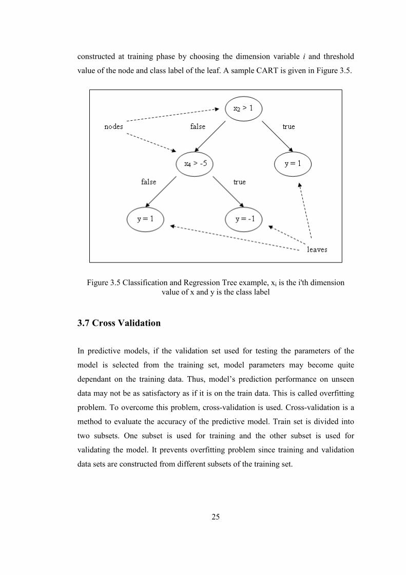
Figure 4.14 Average time domain feature vectors of target (oddball) and non-target (standard) classes obtained by the normalized energy distribution of the signals with

offset trick for channel 11

4.2.2.2 Wigner-Ville Distribution

Integral of WVD over time and frequency gives total energy of the signal. WVD is

also normalized to make total energy of signal equal to 1. In Figure 4.15, all

frequency components of the WVD are summed to get energy distribution over

time. Offset trick is applied to signals before calculating WVD.

45

Figure 4.15 Average time domain feature vectors of target (oddball) and non-target (standard) classes obtained by the sum of all frequency components in WVD for

channel 11.

4.2.2.3 Creating Time-Frequency Domain Features

WVD gives time-frequency analysis of the signals. These signals are converted into

features by dividing WVD into sections and taking averages of each section to

create features. Frequency band is divided according to types of the brain waves.

46

Table 4.1 Brain waves

Type Frequency (Hz) Activity

Delta: ∆ 0.5 – 3.5 Prepare to Motion

Theta: Θ 3.5 – 8 Memory

Alpha (mü): α (µ) 8 – 13 Sensor Idling

Beta: β 13 – 22 Motor Idling

Gamma: γ 22 - 40 Property Fusion

Mean value of each band is calculated to reduce frequency band into 5 components.

Using these 5 components as features causes 5 times increase in feature vector size.

To overcome this problem, time is also divided into uniform sections. For a time

section of length 25 ms, feature vector size reduces 6 times. Averages of time-

frequency domain feature vectors are given in Figure 4.16 for channel 11.

47

Figure 4.16 Average time-frequency domain feature vectors of target (oddball) and non-target (standard) classes obtained from the WVD for channel 11.

4.3 Dimension Reduction

Reducing the size of the data is important to reduce memory usage and processing

time. However, valuable information must be kept while reducing the size of the

data. With a proper dimension reduction, even the classification performance can be

increased by getting rid of irrelevant information.

If same information can be obtained from different channels due to the correlation

of data, then redundancy can be removed by dimension reduction methods.

Correlation of data sampled from different channels at the same instant is measured

to see that if dimension reduction is needed when multiple channel data is used.

Measurement is done by concatenating extracted signals and keeping the

chronological sequence.

48

Correlation coefficients of channel 11 (Cz) with all 64 channels are given in Figure

4.17. Correlation coefficients are greater than 0.8 for neighbor channels (3, 5, 6, 9,

10, 12, 13, 17, 18, and 19) and decreasing with the distance between two channels.

Calculation of correlation coefficients is given in APPENDIX A.

Figure 4.17 Correlation coefficients between channel 11 and other 64 channels

Correlation matrix for channels 3, 4, 5, 10, 11, 12, 17, 18, 19 (placed near to the

center of the skull) are given in Table 4.2. Table 4.2 also shows that channels that

are closer to each other have higher correlation.

49

Table 4.2 Correlation Coefficient Matrix for the subset of channels 3, 4, 5, 10, 11, 12, 17, 18, 19

Channel Number 3 4 5 10 11 12 17 18 19 3 1 0.4 0.9 0.92 0.86 0.88 0.83 0.85 0.79 4 0.4 1 0.39 0.37 0.39 0.38 0.33 0.34 0.32 5 0.9 0.39 1 0.88 0.86 0.93 0.81 0.86 0.84 10 0.92 0.37 0.88 1 0.89 0.91 0.94 0.94 0.87 11 0.86 0.39 0.86 0.89 1 0.9 0.85 0.89 0.84 12 0.88 0.38 0.93 0.91 0.9 1 0.89 0.95 0.94 17 0.83 0.33 0.81 0.94 0.85 0.89 1 0.96 0.9 18 0.85 0.34 0.86 0.94 0.89 0.95 0.96 1 0.96 19 0.79 0.32 0.84 0.87 0.84 0.94 0.9 0.96 1

Correlation coefficient analysis shows that there is a big correlation among some

channels and feature vector size can be reduced by eliminating redundant

information. For this purpose, Principal Component Analysis (PCA) and AdaBoost

are examined in this study as explained below.

4.3.1 Dimension Reduction Using PCA

Dimension reduction with PCA is done by first transforming features into another

space, in which new features are ordered in decreasing variance, and then

eliminating features with small variance. PCA does not consider differences

between classes in data set while reducing dimension. Effect of dimension reduction

using PCA is analyzed for data given channels given in Table 4.2. Filtering and

normalization is not applied to data set. Average feature vectors for target and non-

target intensifications are given in Figure 4.18.

50

Figure 4.18 Average feature vectors of target (oddball) and non-target (standard) classes for channels 3, 4, 5, 10, 11, 12, 17, 18, 19

All feature vectors are transformed using PCA and averages of transformed target

and non-target feature vectors are given in Figure 4.19. Dimension reduction is not

done after transformation. Because of that, feature vector size is equivalent with

non-transformed feature vectors given in Figure 4.18.

51

Figure 4.19 Average PCA transformed feature vectors of target (oddball) and non-target (standard) classes for channels 3, 4, 5, 10, 11, 12, 17, 18, 19

Information kept while reducing the dimensionality in PCA is calculated with:

100

1

1 ×=

∑

∑

=

=n

i

i

p

i

i

r

λ

λ, (4-2)

where λi is the eigenvalue of the i’th feature, n is the number of features and p is the

reduced feature number. In Figure 4.20, change of r with p is shown for the feature

vectors analyzed in Figure 4.19.

52

0

20

40

60

80

100

120

1 101 201 301 401 501 601 701 801 901 1001

reduced feature number, p

r

Figure 4.20 Percentage of information kept (r) vs. number of feature components included (p) for channels 3, 4, 5, 10, 11, 12, 17, 18, 19

In Figure 4.20, dimension of the feature vector to keep 90% of the information is

found to be the first 91 features of PCA transformed feature vectors. In Figure 4.21,

average target and non-target PCA transformed feature vectors with 91 components

are given.

53

Figure 4.21 Average PCA transformed and reduced feature vectors of target (oddball) and non-target (standard) classes for channels 3, 4, 5, 10, 11, 12, 17, 18,

19

4.3.2 Dimension Reduction Using AdaBoost

AdaBoost selects features using the discriminative properties of the target and non-

target classes. AdaBoost does not transform features during selection. It only

determines a subset of features using the information provided in training data. That

is, dimension reduction via AdaBoost is performed by eliminating unselected

features from feature vectors. Because of that, calculation overhead does not exist

after system is trained. In Figure 4.22, first 30 features of channel 11 selected by

AdaBoost with CART as the weak classifier are marked on average target and non-

target classes. Selected features are sorted according to their selection order in

Figure 4.23.

54

Figure 4.22 30 features selected by AdaBoost from channel 11; selected features are marked with ‘o’ on both averages of target (oddball) and non-target (standard)

classes

55

Figure 4.23 Averages of target (oddball) and non-target (standard) classes for the first 30 features selected by AdaBoost; features are given in selection order and

selected from channel 11

4.4 Classification

Classification is done in two steps. In first step, binary classification is done to

decide if the feature vectors belong to target or non-target classes. In second step,

decision fusion is done to select a target character using binary classification results.

4.4.1 Binary Classification

In binary classification, each feature vector is processed independently and labeled

as either target or non-target classes. SVM and AdaBoost binary classification

methods are used to classify features. 5-fold CV is used in both methods to prevent

overfitting problem.

56

4.4.1.1 Support Vector Machine

SVM is trained using all of the train feature vectors. Soft Margin SVM is used to

introduce a penalty or regularization parameter (C) for misclassified samples. This

parameter is used to tune the system to increase classification performance. Also,

Gaussian Radial Basis Function (RBF) is used as kernel. Gaussian RBF brings an

extra control parameter σ to SVM which provides more suitable boundary selection.

5-fold cross validation is used to tune SVM control parameters (C,σ) and prevent

overfitting problem. Soft margin outputs of cross validation results are summed and

label of the feature vector is decided. For every label, a label rate showing the

strength of the guess is also provided using the summation of cross validation soft

margin results.

4.4.1.2 AdaBoost

AdaBoost learns data using the whole train data set with cross validation. AdaBoost

maximum iteration number is the only parameter that needs to be adjusted

according to the data set. AdaBoost mislabeled target and non-target feature vectors

rate is saturated after maximum iteration number becomes sufficiently large. So,

once maximum iteration number is properly selected, AdaBoost can adapt to data

set without requiring any other adjustments. CART is used as the weak classifier of

the AdaBoost. In Figure 4.24, binary classification error of AdaBoost is given up to

maximum iteration number 200. So, maximum iteration of 100 is sufficiently large

to reach saturation point. Binary classification outputs of cross validation results are

summed and label of the feature vector is decided. For every label, a label rate

showing the strength of the guess is also provided using the summation of cross

validation binary classification results.

57

Figure 4.24 AdaBoost Iteration number vs. error rate graphics for channels 9,11,13,34,49,51,53,56,60,62

4.4.2 Decision Fusion

Target character is selected among 36 characters using binary classification results

with a voting based decision fusion. Binary classification gives target/non-target

classification results for 6 rows and 6 columns but only one of the rows and

columns include the target character. To select a row and a column, repetitions of

the target character are used. There can be up to 15 repetitions for each character.

The possibility of being target row/column is found using the label rate of each

binary classification. Then, repetition results are combined by summing this value

for each row and column and the row and the column with the maximum possibility

are selected as target row and column. Then, interception of the row and the column

gives the target character. Note that it is important to classify target character with

less number of repetitions to increase the usability of the system.

58

CHAPTER 5

EXPERIMENTAL RESULTS

Designed system is composed of three main steps called as preprocessing data,

creating feature vectors and classification. Data is extracted using relevant channels

and filtered at preprocessing step. Then, data is transformed into feature space,

normalized, and its dimensionality is reduced to obtain feature vectors in next step.

At final step, binary classification of the feature vectors are done and target

character is predicted. Overview of the designed system is given in Figure 5.1.

Figure 5.1 Overview of the designed system

First, filtering and normalization methods that best fit on transformation methods

are selected. Then, optimum channels are selected using binary classification

methods for each transformation method. Classification performances of

transformation methods are evaluated and channel subset, transformation method

59

and binary classification method that gives maximum classification performance is

determined. Then, effect of dimension reduction methods on feature vectors is

analyzed. Finally, character prediction results are analyzed with the designed

method.

First of all, performance measurement criteria are required while training and

testing the system. Because of that, this chapter starts with explanation of evaluation

criteria used while measuring performance of the methods and then continues with

the outputs of the experimental results.

At training step, 5-fold Cross Validation (CV) results are used as success criteria.

At each fold of CV, while 80% of data is used for training, the remaining 20% of

data is used only for testing purpose to prevent overfitting. This is repeated 5 times,

keeping a different 20% portion of data for validation. Success criterion is obtained

by averaging classification results of these validation sets. For example, average

misclassification rate of the sample CV result given in Table 5.1 is 16.79%. This

means that %83.21 of test set labels are classified correctly. Aim is to maximize

classification rate or minimize misclassification/error rate of the averaged CV

results.

Table 5.1 Sample Cross Validation misclassification rates for 5-fold cross validation

CV fold-1 CV fold-2 CV fold-3 CV fold-4 CV fold-5

16.87% 16.27% 17.66% 14.29% 18.85%

Each CV result is calculated by first counting True Positive (TP), False Negative

(FN), True Negative (TN), and False Positive (FP) samples, where meanings of TP,

FN, TN, and FP are given as:

True Positive (TP): Number of correctly labeled target feature vectors

False Negative (FN): Number of mislabeled target feature vectors

60

True Negative (TN): Number of correctly labeled non-target feature vectors

False Positive (FP): Number of mislabeled non-target feature vectors

Then, sensitivity (True Positive Rate) given in (5-1) and specificity (True Negative

Rate) given in (5-2) are calculated.

FNTP

TPTPRveRateTruePositi

+=)( (5-1)

FPTN

TNTNRveRateTrueNegati

+=)( (5-2)

Finally TPR and TNR results are averaged (see (5-3)) to obtain success of the

classification.

2)(

TNRTPRSReSuccessRat

+= (5-3)

Equivalently, error rate can be also obtained by using the success rate of the

classification (see (5-4)).

SRERErrorRate −= 1)( (5-4)

In train set, number of non-target samples is reduced by random selection to have

equal number of target samples (TP + FN) and non-target samples (TN + FP).

Overall classification performance is also evaluated using (5-4) on a separate test

set that is not used in CV. Since character detection is done on test set, number of

non-target samples is not reduced by random selection. Because of that, there are 5

times more non-target samples than target samples in test set. Weight of target and

non-target samples on success criteria is equalized by using (5-3).

Another performance criterion, which is named as Quality Rate (5-5), is maximized

at channel selection.

61

FNFPTP

TPQReQualityRat

++=)( (5-5)

Equivalently, Quality Error Rate (5-6) can also be minimized instead of

maximizing (5-5).

FNFPTP

FNFPQRQERorRateQualityErr

+++

=−= 1)( (5-6)

As it is stated before, there are 5 non-target samples for each target sample in test

set. Because of that, importance of target feature classification is increased by

omitting TN while evaluating the performance of the classification at channel

selection. Equation (5-5) is also used by Rakotomamonjy [30] while selecting

channels in his study. 5-fold cross-validation is also used at channel selection to

prevent overfitting.

After individual prediction of target and non-target samples, target character

prediction is done. Character recognition performance is evaluated by dividing

correctly classified target characters to total character numbers.

Note that all performance evaluation formulas, (5-1), (5-2), (5-3), (5-4), (5-5) and

(5-6), take values between 0 and 1.

5.1 Analyzing Effects of Filtering and Normalization Methods on

Time and Time-Frequency Domain Signals

There are two types of filtering that are applied to data set. First one is applying a

band-pass filter without changing the sampling rate and second one is down-

sampling data by averaging consecutive samples. Applying band-pass filter is

optional and can be skipped. However, down-sampling, which is applied at the end

of filtering step of Preprocess, is not optional. Data is sampled at 240 Hz. However,

maximum frequency which is required for Time-Frequency Domain features is 40

Hz. In order to reduce the dimension of the data and get rid of high frequency signal

components, data is down-sampled to 40 Hz by averaging the observations with

62

non-overlapping windows. That is, at the end of filtering, each 6 sample is averaged

and represented as a single value. So, data is both filtered and its size is reduced 6

times by down-sampling.

The word “filtering” represents applying band-pass filter without changing

sampling rate. Since down-sampling is always implemented, it is excluded from

“filtering” definition.

First, effects of filtering and normalization on Time and Time-Frequency signals are

analyzed to find out the best combination in terms of classification. Also, optimum

control parameters (C,σ) for SVM are found for each combination. These decisions

are done using reference channels used by Kaper et al. [24] and Erdoğan et al. [29]

and all repetitions. Overview of applied method is given in Figure 5.2.

Figure 5.2 Schematic of filtering and normalization analysis

Basic settings given in Table 5.2 are applied to all channels while evaluating the

methods. Configurable settings are summarized in Table 5.3. Results of the analysis

are given in Table 5.4. As it is seen from the results, best performance for time

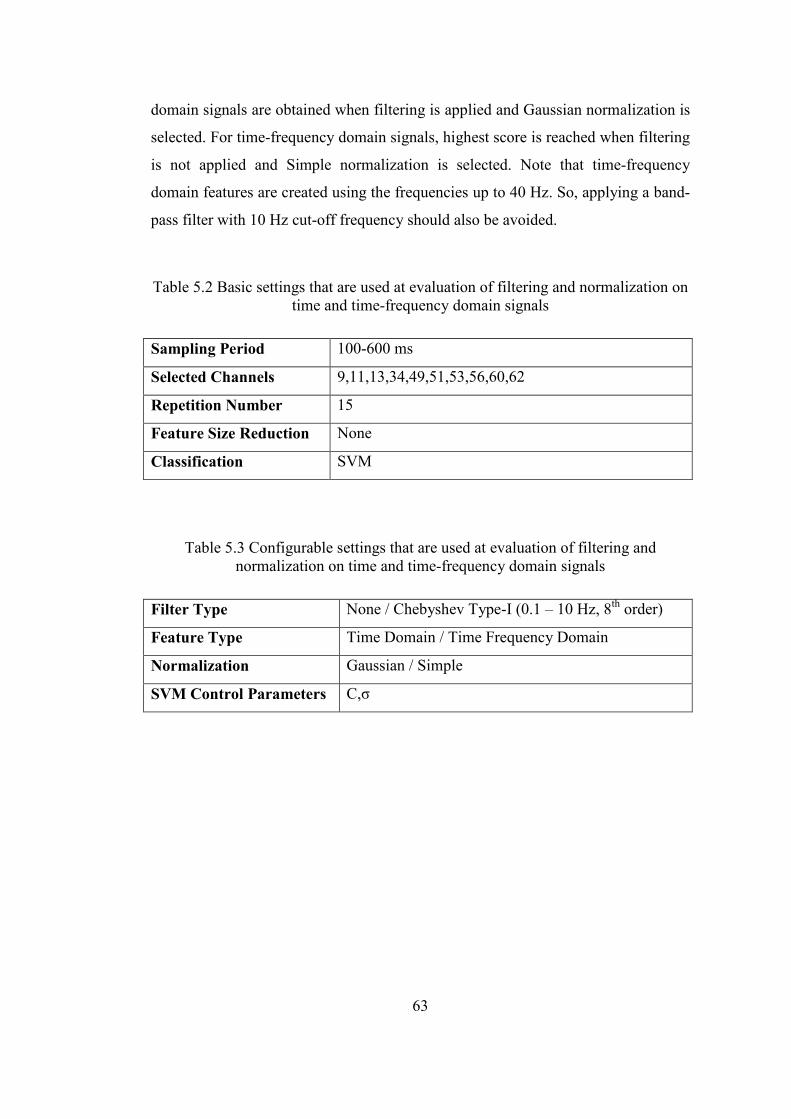
63

domain signals are obtained when filtering is applied and Gaussian normalization is

selected. For time-frequency domain signals, highest score is reached when filtering

is not applied and Simple normalization is selected. Note that time-frequency

domain features are created using the frequencies up to 40 Hz. So, applying a band-

pass filter with 10 Hz cut-off frequency should also be avoided.

Table 5.2 Basic settings that are used at evaluation of filtering and normalization on time and time-frequency domain signals

Sampling Period 100-600 ms

Selected Channels 9,11,13,34,49,51,53,56,60,62

Repetition Number 15

Feature Size Reduction None

Classification SVM

Table 5.3 Configurable settings that are used at evaluation of filtering and normalization on time and time-frequency domain signals

Filter Type None / Chebyshev Type-I (0.1 – 10 Hz, 8th order)

Feature Type Time Domain / Time Frequency Domain

Normalization Gaussian / Simple

SVM Control Parameters C,σ

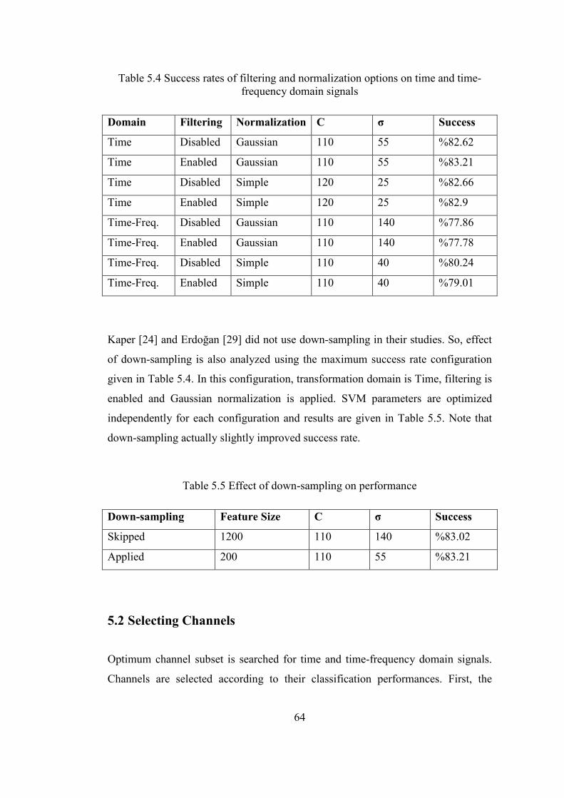
64

Table 5.4 Success rates of filtering and normalization options on time and time-frequency domain signals

Domain Filtering Normalization C σ Success

Time Disabled Gaussian 110 55 %82.62

Time Enabled Gaussian 110 55 %83.21

Time Disabled Simple 120 25 %82.66

Time Enabled Simple 120 25 %82.9

Time-Freq. Disabled Gaussian 110 140 %77.86

Time-Freq. Enabled Gaussian 110 140 %77.78

Time-Freq. Disabled Simple 110 40 %80.24

Time-Freq. Enabled Simple 110 40 %79.01

Kaper [24] and Erdoğan [29] did not use down-sampling in their studies. So, effect

of down-sampling is also analyzed using the maximum success rate configuration

given in Table 5.4. In this configuration, transformation domain is Time, filtering is

enabled and Gaussian normalization is applied. SVM parameters are optimized

independently for each configuration and results are given in Table 5.5. Note that

down-sampling actually slightly improved success rate.

Table 5.5 Effect of down-sampling on performance

Down-sampling Feature Size C σ Success

Skipped 1200 110 140 %83.02

Applied 200 110 55 %83.21

5.2 Selecting Channels

Optimum channel subset is searched for time and time-frequency domain signals.

Channels are selected according to their classification performances. First, the

65

channel with best classification performance is selected. Then, rest of the channels

is considered and the one giving the best classification performance when

concatenated to previously selected channel is selected. Channels are sorted by

concatenating all remaining channels one by one with previously selected ones until

32 out of 64 channels are sorted. Both SVM and AdaBoost methods are used to find

out classification performance at channel selection. AdaBoost results are obtained

with the weak classifier CART. Overview of the channel selection methods are

given in Figure 5.3.

Figure 5.3 Schematic of channel selection methods

AdaBoost classification parameters do not depend on data set. However, as it is

seen from section 5.1, SVM parameters highly depend on data set. Parameters

obtained at section 5.1 are used for SVM classification. Error is plotted according to

the equation given in (5-6) for each number of selected channels and optimum

number of channels to be used is selected accordingly in the following sections.

Channel selection completion time is also given for each configuration. PC used for

channel selection has dual core 3.00 GHz CPU and 4 GB RAM.

66

5.2.1 Time Domain and AdaBoost Channel Selection

AdaBoost channel selection order for Time Domain signals is given in Table 5.6.

Completion of 32 channel selection takes 124 hours or equivalently 5.17 days. First

10 channels are shown in Figure 5.4.

Table 5.6 Selected channels for Time Domain and AdaBoost configuration

Order 1 2 3 4 5 6 7 8

Channel ID 9 56 51 60 6 17 28 18

Order 9 10 11 12 13 14 15 16

Channel ID 62 46 55 61 14 44 49 38

Order 17 18 19 20 21 22 23 24

Channel ID 7 52 21 58 27 1 20 3

Order 25 26 27 28 29 30 31 32

Channel ID 2 29 40 47 50 35 30 41

67

Figure 5.4 Selected 10 channels for Time Domain and AdaBoost configuration

Figure 5.5 shows that using first 12 channels is sufficient and adding more channels

actually does not improve the result. QER is 0.33 for first 10 channels and 0.323 for

first 12 channels.

68

Time Domain & AdaBoost Channel Selection

0

0,1

0,2

0,3

0,4

0,5

0,6

1 2 3 4 5 6 7 8 9 10 11 12 13 14 15 16 17 18 19 20 21 22 23 24 25 26 27 28 29 30 31 32

Selected Channel No

Quality Error Rate

Figure 5.5 Quality Error Rate vs. number of selected channels for Time Domain and AdaBoost configuration

5.2.2 Time Domain and SVM Channel Selection

SVM channel selection order for Time Domain signals is given in Table 5.7.

Completion of 32 channel selection takes 12 hours. First 10 channels are shown in

Figure 5.6.

Table 5.7 Selected channels for Time Domain and SVM configuration

Order 1 2 3 4 5 6 7 8

Channel ID 10 60 51 56 3 64 18 54

Order 9 10 11 12 13 14 15 16

Channel ID 59 63 45 49 58 61 55 42

Order 17 18 19 20 21 22 23 24

Channel ID 4 6 9 53 17 1 19 40

Order 25 26 27 28 29 30 31 32

Channel ID 12 26 34 16 46 21 48 32

69

Figure 5.6 Selected 10 channels for Time Domain and SVM configuration

Figure 5.7 shows that using first 22 channels is sufficient. QER is 0.273 for first 10

channels and 0.226 for first 22 channels.

70

Time Domain & SVM Channel Selection

0

0,1

0,2

0,3

0,4

0,5

0,6

1 2 3 4 5 6 7 8 9 10 11 12 13 14 15 16 17 18 19 20 21 22 23 24 25 26 27 28 29 30 31 32

Selected Channel No

Quality Error Rate

Figure 5.7 Quality Error Rate vs. number of selected channels for Time Domain and SVM configuration

5.2.3 Time-Frequency Domain and SVM Channel Selection

SVM channel selection order for Time-Frequency Domain signals is given in Table

5.8. Completion of 32 channel selection takes 52 hours. First 10 channels are shown

in Figure 5.6.

Table 5.8 Selected channels for Time Domain and SVM configuration

Order 1 2 3 4 5 6 7 8

Channel ID 11 60 18 52 56 41 62 58

Order 9 10 11 12 13 14 15 16

Channel ID 48 54 40 59 8 42 64 9

Order 17 18 19 20 21 22 23 24

Channel ID 55 61 25 17 10 51 63 1

Order 25 26 27 28 29 30 31 32

Channel ID 16 46 2 3 57 7 44 13

71

Figure 5.8 Selected 10 channels for Time-Frequency Domain and SVM configuration

Figure 5.7 shows that using first 21 channels is sufficient. QER is 0.31 for first 10

channels and 0.285 for first 21 channels.

72

Time-Frequency Domain & SVM Channel Selection

0

0,1

0,2

0,3

0,4

0,5

0,6

1 2 3 4 5 6 7 8 9 10 11 12 13 14 15 16 17 18 19 20 21 22 23 24 25 26 27 28 29 30 31 32

Selected Channel No

Quality Error Rate

Figure 5.9 Quality Error Rate vs. number of selected channels for Time-Frequency Domain and SVM configuration

5.2.4 Time-Frequency Domain and AdaBoost Channel Selection

Time-Frequency Domain and AdaBoost channel selection configuration is skipped

due to the expected completion of 32 channels selection time. Length of Time-

Frequency Domain features are 5 times more than Time Domain features. AdaBoost

channel selection linearly increases with data length. So, expected completion time

of Time-Frequency Domain and AdaBoost channel selection is 124*5 = 620 hours,

or equivalently 25.83 days.

Effects of skipping Time-Frequency Domain and AdaBoost channel selection is

analyzed in 5.2.5.

5.2.5 Evaluation of Channel Selection Methods

Classification performances of 10 channels used by Kaper et al. [24] and Erdoğan et

al. [29] are used as reference while evaluating channel selection methods.

Classification results for 10 channels and optimum number of channels are

compared with reference results. Performances are evaluated in terms of both

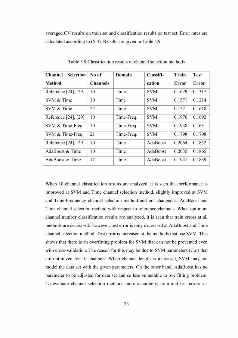
73

averaged CV results on train set and classification results on test set. Error rates are

calculated according to (5-4). Results are given in Table 5.9.

Table 5.9 Classification results of channel selection methods

Channel Selection

Method

No of

Channels

Domain Classifi-

cation

Train

Error

Test

Error

Reference [24], [29] 10 Time SVM 0.1679 0.1317

SVM & Time 10 Time SVM 0.1571 0.1214

SVM & Time 22 Time SVM 0.127 0.1618

Reference [24], [29] 10 Time-Freq. SVM 0.1976 0.1692

SVM & Time-Freq. 10 Time-Freq. SVM 0.1948 0.163

SVM & Time-Freq. 21 Time-Freq. SVM 0.1798 0.1798

Reference [24], [29] 10 Time AdaBoost 0.2064 0.1852

AdaBoost & Time 10 Time AdaBoost 0.2035 0.1865


When 10 channel classification results are analyzed, it is seen that performance is

improved at SVM and Time channel selection method, slightly improved at SVM

and Time-Frequency channel selection method and not changed at AdaBoost and

Time channel selection method with respect to reference channels. When optimum

channel number classification results are analyzed, it is seen that train errors at all

methods are decreased. However, test error is only decreased at AdaBoost and Time

channel selection method. Test error is increased at the methods that use SVM. This

shows that there is an overfitting problem for SVM that can not be prevented even

with cross-validation. The reason for this may be due to SVM parameters (C,σ) that

are optimized for 10 channels. When channel length is increased, SVM may not

model the data set with the given parameters. On the other hand, AdaBoost has no

parameter to be adjusted for data set and so less vulnerable to overfitting problem.

To evaluate channel selection methods more accurately, train and test errors vs.

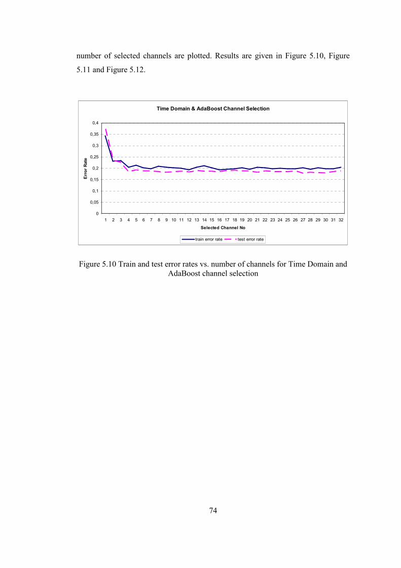
74

number of selected channels are plotted. Results are given in Figure 5.10, Figure

5.11 and Figure 5.12.

Time Domain & AdaBoost Channel Selection

0

0,05

0,1

0,15

0,2

0,25

0,3

0,35

0,4

1 2 3 4 5 6 7 8 9 10 11 12 13 14 15 16 17 18 19 20 21 22 23 24 25 26 27 28 29 30 31 32

Selected Channel No

Error Rate

train error rate test error rate

Figure 5.10 Train and test error rates vs. number of channels for Time Domain and AdaBoost channel selection

75

Time Domain & SVM Channel Selection

0

0,05

0,1

0,15

0,2

0,25

0,3

0,35

0,4

1 2 3 4 5 6 7 8 9 10 11 12 13 14 15 16 17 18 19 20 21 22 23 24 25 26 27 28 29 30 31 32

Selected Channel No

Error Rate


Figure 5.11 Train and test error rates vs. number of channels for Time Domain and SVM channel selection

Time-Frequency Domain & SVM Channel Selection

0

0,05

0,1

0,15

0,2

0,25

0,3

0,35

0,4

1 2 3 4 5 6 7 8 9 10 11 12 13 14 15 16 17 18 19 20 21 22 23 24 25 26 27 28 29 30 31 32

Selected Channel No

Error Rate


Figure 5.12 Train and test error rates vs. number of channels for Time-Frequency Domain and SVM channel selection

In Figure 5.10, AdaBoost and Time channel selection method train and test error

behaviors are similar. On the other hand, in Figure 5.11 and Figure 5.12, train and

test error behaviors are different. Train error bottom point is around 20 channels and

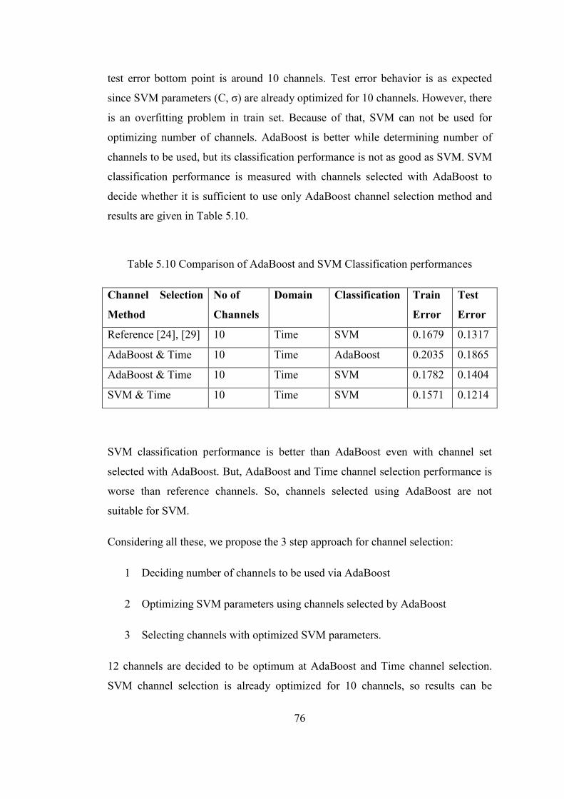
76

test error bottom point is around 10 channels. Test error behavior is as expected

since SVM parameters (C, σ) are already optimized for 10 channels. However, there

is an overfitting problem in train set. Because of that, SVM can not be used for

optimizing number of channels. AdaBoost is better while determining number of

channels to be used, but its classification performance is not as good as SVM. SVM

classification performance is measured with channels selected with AdaBoost to

decide whether it is sufficient to use only AdaBoost channel selection method and

results are given in Table 5.10.

Table 5.10 Comparison of AdaBoost and SVM Classification performances

Channel Selection

Method

No of

Channels

Domain Classification Train

Error

Test

Error



AdaBoost & Time 10 Time SVM 0.1782 0.1404

SVM & Time 10 Time SVM 0.1571 0.1214

SVM classification performance is better than AdaBoost even with channel set

selected with AdaBoost. But, AdaBoost and Time channel selection performance is

worse than reference channels. So, channels selected using AdaBoost are not

suitable for SVM.

Considering all these, we propose the 3 step approach for channel selection:

1 Deciding number of channels to be used via AdaBoost

2 Optimizing SVM parameters using channels selected by AdaBoost

3 Selecting channels with optimized SVM parameters.

12 channels are decided to be optimum at AdaBoost and Time channel selection.

SVM channel selection is already optimized for 10 channels, so results can be

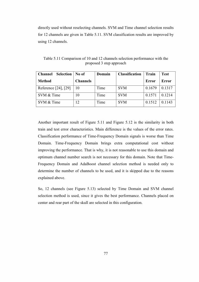
77

directly used without reselecting channels. SVM and Time channel selection results

for 12 channels are given in Table 5.11. SVM classification results are improved by

using 12 channels.

Table 5.11 Comparison of 10 and 12 channels selection performance with the proposed 3 step approach

Channel Selection

Method

No of

Channels

Domain Classification Train

Error

Test

Error


SVM & Time 10 Time SVM 0.1571 0.1214

SVM & Time 12 Time SVM 0.1512 0.1143

Another important result of Figure 5.11 and Figure 5.12 is the similarity in both

train and test error characteristics. Main difference is the values of the error rates.

Classification performance of Time-Frequency Domain signals is worse than Time

Domain. Time-Frequency Domain brings extra computational cost without

improving the performance. That is why, it is not reasonable to use this domain and

optimum channel number search is not necessary for this domain. Note that Time-

Frequency Domain and AdaBoost channel selection method is needed only to

determine the number of channels to be used, and it is skipped due to the reasons

explained above.

So, 12 channels (see Figure 5.13) selected by Time Domain and SVM channel

selection method is used, since it gives the best performance. Channels placed on

center and rear part of the skull are selected in this configuration.

78

Figure 5.13 12 channels selected by Time Domain and SVM channel selection method

Configuration parameters that are determined up to now are summarized in Table

5.12.

Table 5.12 Fixed configuration parameters after channel selection

Sampling Period 100-600 ms, 40 Hz down-sampled

Selected Channels 3, 10, 18, 45, 49, 51, 54, 56, 59, 60, 63, 64

Filter Type Chebyshev Type-I (0.1 – 10 Hz, 8th order)

Feature Type Time Domain

Normalization Gaussian

Classification SVM (C=110,σ=55)

79

5.3 Reducing Dimension of the Features

Feature dimension is already reduced 6 times at down-sampling. In this section, the

effect of further reducing dimension of features is analyzed. PCA and AdaBoost

feature selection methods are used at analysis. CART is used as the weak classifier

of the AdaBoost. Overview of the analysis method, which uses the fixed

configuration parameters given in Table 5.12, is given in Figure 5.14.

Figure 5.14 Schematic of dimensionality reduction methods

PCA does not reduce the number features used as input to the system when it is

used for dimension reduction. PCA reduces the dimension through a transformation

at an intermediate step. That is, PCA must be applied to both train and test set

feature vectors. Also, PCA does not consider class labels in data set while reducing

dimension. On the other hand, AdaBoost is a feature selection method. So, the

number of features used as input to the system can be reduced by AdaBoost. That

is, once subset of features are determined at training, train and test set features are

easily created by getting rid of unselected features without any calculation effort.

80

Besides, AdaBoost selects features by taking into account discriminative properties

of classes.

5.3.1 Dimensionality Reduction Using PCA

PCA eigenvalue ratio which is calculated according to Equation (4-2) is given in

Figure 5.15. First 100 and 160 features contain 99.5% and %99.97 of the data

respectively. So, there are correlated features in feature vectors.

0

20

40

60

80

100

120

1 21 41 61 81 101 121 141 161 181 201 221

reduced feature number, p

r

Figure 5.15 Percentage of information kept (r) vs. number of feature components included (p) for selected 12 channels

In Figure 5.16, train and test error rates vs. number of selected features are given.

As expected, eigenvalue ratio and error characteristics are similar. First 160 PCA

features contain all of the information and give same classification results with

using all features.

81

PCA Feature Dimension Reduction

0

0,05

0,1

0,15

0,2

0,25

20 40 60 80 100 120 140 160 180 200 220 240

Selected Feature No

Error Rate


Figure 5.16 PCA dimension reduction results

5.3.2 Dimensionality Reduction Using AdaBoost

AdaBoost dimension reduction results are given in Figure 5.17. Error rates are first

decreasing and then saturating with increasing number of features. Minimum error

rate is observed when all features are selected. So, reducing the feature number

increases error rate.

82

AdaBoost Feature Dimension Reduction

0

0,02

0,04

0,06

0,08

0,1

0,12

0,14

0,16

0,18

0,2

20 40 60 80 100 120 140 160 180 200 220 240

Selected Feature No

Error Rate


Figure 5.17 AdaBoost dimension reduction results

5.3.3 Evaluation of Dimensionality Reduction

When error rates given in Figure 5.16 and Figure 5.17 are compared, it is seen that

AdaBoost feature selection results are better for less than 120 features and PCA

feature selection results are better for more than 120 features. PCA assumes that

features with larger variances contain more important information and reduces data

with this principle. Note that PCA is a transformation method and it successfully

eliminates correlated features. Since first 100 PCA features already contains 99.5%

of the data variance, eliminating rest of the features removes correlation. On the

other hand, AdaBoost selects features using discriminative properties of classes.

Since features with smaller variance can also contain valuable information while

separating classes, AdaBoost is more powerful at smaller number of features.

However, AdaBoost gains less information with increasing number features because

it does not transform features.

AdaBoost always loses some information because error rates are increased with

AdaBoost dimensionality reduction. However, PCA reduces feature size by 80

without losing performance by getting rid of correlated variables. In order not to

83

increase error rates, PCA is selected as dimensionality reduction method with

feature size 160.

If one needs to further reduce the dimension of the features, it can combine

powerful sides of both methods by first applying PCA and getting rid of correlated

data and then applying AdaBoost to further reduce data size.

5.4 Classifying Features and Deciding Focused Characters

Superiority of SVM over AdaBoost is already shown during channel selection.

Because of that, only SVM is used while classifying features. Target (or focused)

characters are selected based on voting according to soft margin outputs of SVM.

There are total 42 characters in train set and 31 characters in test set provided in

[20]. Trained SVM is both tested on 42 character train set and 31 character test set.

Performance is measured by dividing correctly classified target characters to total

character numbers. Results are given for both reference channels used by Kaper

[24] and 12 channels selected by SVM in time domain. Performance of target

character detection is measured for repetition numbers from 1 to all. Repetitions are

selected in chronological order. In Figure 5.18, results of train set and reference

channels are given. In Figure 5.19, results of train set and 12 channels selected by

SVM are given. In Figure 5.20, results of test set and reference channels are given.

In Figure 5.21, results of test set and 12 channels selected by SVM are given.

When Figure 5.18 and Figure 5.19 are compared, it is seen that selected channels

give better performance results than reference channels. Note that a character is

always misclassified by both channel sets. Character ‘G’ is always found instead of

‘H’ in second “HAT” word of train set. This character can be dismissed from train

set. Erdoğan [29] already constructed train set with 39 characters and did not use

this misclassified character.

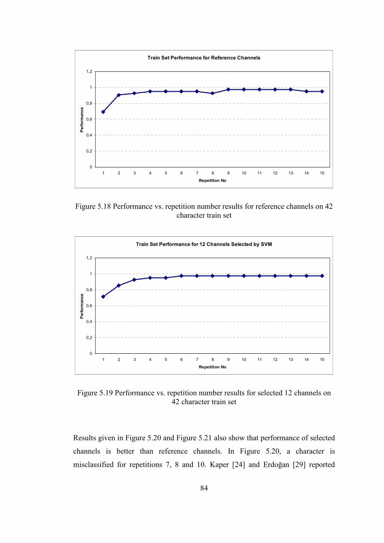
84

Train Set Performance for Reference Channels

0

0,2

0,4

0,6

0,8

1

1,2

1 2 3 4 5 6 7 8 9 10 11 12 13 14 15

Repetition No

Performance

Figure 5.18 Performance vs. repetition number results for reference channels on 42 character train set

Train Set Performance for 12 Channels Selected by SVM

0

0,2

0,4

0,6

0,8

1

1,2

1 2 3 4 5 6 7 8 9 10 11 12 13 14 15

Repetition No

Performance

Figure 5.19 Performance vs. repetition number results for selected 12 channels on 42 character train set

Results given in Figure 5.20 and Figure 5.21 also show that performance of selected

channels is better than reference channels. In Figure 5.20, a character is

misclassified for repetitions 7, 8 and 10. Kaper [24] and Erdoğan [29] reported

85

%100 performance for these repetitions. There are numerous factors, such as

randomly selected train set and soft margin outputs of SVM, that may affect the

performance results. However, only variable is channel subset in the experiment

and thus comparison of channel sets are done under same conditions.

Test Set Performance for Reference Channels

0

0,2

0,4

0,6

0,8

1

1,2

1 2 3 4 5 6 7 8 9 10 11 12 13 14 15

Repetition No

Performance

Figure 5.20 Performance vs. repetition number results for reference channels on 31 character test set

86

Test Set Performance for 12 Channels Selected by SVM

0

0,2

0,4

0,6

0,8

1

1,2

1 2 3 4 5 6 7 8 9 10 11 12 13 14 15

Repetition No

Performance

Figure 5.21 Performance vs. repetition number results for selected 12 channels on 31 character test set

87

CHAPTER 6

CONCLUSIONS

In this thesis, Spelling Paradigm, a specific implementation of BCI, is studied. P300

signals are collected from different parts of the brain. Using all collected data slows

down the system and increases the noise level because P300 response does not exist

at same intensity at all regions of the brain. Channel subset that contains relevant

data with minimum noise is searched. AdaBoost with the weak classifier CART and

SVM classification methods are used in this study. Besides, P300 responses are

analyzed in time and time-frequency domains. Best subset of channels is analyzed

for the combinations of classification and transformation domain methods. Since

SVM parameters (C, σ) depend on data set, it needs optimization before starting the

analysis. So, number of channels to be used and a channel subset is required before

starting the analysis. Using a reference subset of channels can not solve this

problem, because although SVM gives successful results around the region that its

parameters are optimized, it loses its learning ability at other regions and can not

model data set properly. On the other hand, AdaBoost does not require parameter

optimization for each subset of data and suitable to detect optimum subset of

channels. However, AdaBoost with the weak classifier CART classification

performance is worse than the optimized SVM and so it is wise to select SVM as

primary classification method of the system. Success of SVM classification with

channels selected by AdaBoost is analyzed and it is seen that SVM is more

successful if channels are also selected by SVM. So, AdaBoost is better while

deciding number of channels to be used and SVM is better at classification. Strong

sides of both methods are combined while selecting channels by deciding number of

88

channels to be used via AdaBoost channel selection method and optimizing SVM

with the channel subset selected with AdaBoost and reselecting channels with

optimized SVM parameters.

P300 signals are analyzed in time and time-frequency domains. Filtering and

normalization methods that best suits for these domains are analyzed. It is decided

to use time domain with filtering and Gaussian normalization and time-frequency

domain without filtering and simple normalization. Since signals already exist in

time domain, no transformation is required for time domain analysis. To transform

time domain signals into time-frequency domain, WVD is used. Frequency band of

WVD output is divided according to the types of brain waves namely delta, theta,

alpha, beta, and gamma. Averages of WVD for each brain wave type are calculated

and results are concatenated to create feature vectors. Since there are five brain

wave types, feature vector size is five times of the one obtained from time domain.

After channel selection analysis is done, it is observed that time domain is both

cheaper in terms of computational effort and better in terms of classification. So,

time domain is preferred as the primary transformation domain.

In time domain, AdaBoost selects 12 as the optimum number of channels to be

used. 12 channels selected by SVM are 3, 10, 18, 45, 49, 51, 54, 56, 59, 60, 63, and

64. Classification results are compared with 10 reference channels used by Kaper

[24], and Erdoğan [29]. Train and test errors are found to be 0.1679 and 0.1317

respectively for reference channels and 0.1512 and 0.1143 respectively for 12

selected channels. So, channel selection method improved the classification

performance of the system.

Dimension is tried to be reduced without decreasing the success of the

implementation. 100 – 600 ms period after intensification is used for each channel.

Since signals are sampled at 240 Hz, there are total 120 features for each channel.

Total feature size becomes 1440 for 12 channels. This increases training time and

also may cause memory errors with the increasing number of samples. It is shown

that downsampling signals to 40 Hz do not cause information loss at all. Also, PCA

and AdaBoost with the weak classifier CART dimension reduction methods are

89

analyzed. PCA successfully eliminates correlated data. However, it is not as

successful as AdaBoost if feature size is further reduced. This due to the fact that

AdaBoost takes into account discriminative properties of classes, but PCA does not

consider this information. AdaBoost dimension reduction always increases error

rates in comparison to full set and not preferred. PCA reduces feature size up to 160

without any information loss. So, PCA is selected as dimension reduction method.

If further dimension reduction is needed, then information loss should be minimized

by first getting rid of correlated features by PCA and then applying AdaBoost to the

feature set already reduced by PCA.

As it is stated before, SVM is used for labeling test set feature vectors due to its

superior performance over AdaBoost with the weak classifier CART. Margin

outputs of SVM are used while selecting target rows and columns. Then target

character is decided combining target rows and columns. Effect of reducing

repetition numbers on performance of system is also analyzed and it is seen that 12

channels selected by SVM in time domain gives also better results.

Note that since brain signals up to 40 Hz are required for time-frequency analysis,

downsampling frequency is selected to be 40 Hz in this study. Results already show

that time domain features are preferred against time-frequency domain signals. So,

downsampling frequency can be further reduced and information loss can be

analyzed.

In this study, CART is used as the weak classifier of the AdaBoost. Different weak

classifiers can be analyzed to improve the classification and dimension reduction

performance of the AdaBoost. If AdaBoost with another weak classifier gives better

classification results than SVM, then it can be used at classification step in addition

to the decision of the number of channels to be used. That is, the necessity to use

SVM can be eliminated by improving the classification performance of the

AdaBoost.

In this study, rows and columns are processed together. Effects of separating rows

and columns while processing signals can be analyzed.

90

In this study, standard filter is used at preprocessing step. Adaptive filters such as

Wiener filter can be implemented.

91

REFERENCES

[1] J. J. Vidal, “Real-time detection of brain events in EEG,” Proc.

IEEE, vol. 65, pp. 633–664, May 1977

[2] G. Pfurtscheller, D. Flotzinger,W. Mohl, and M. Peltoranta,

“Prediction of the side of hand movements from single-trial multi-channel

EEG-data using neural networks,” Electroencephalgr. Clin. Neurophysiol.,

vol. 82, pp. 313–315, 1992

[3] G. Pfurtscheller, C. Neuper,A. Schloegl, and K. Lugger,

“Separability of EEG signals recorded during right and left motor imagery

using adaptive autoregressive parameters,” IEEE Trans. Rehab. Eng., vol. 6,

pp. 316–325, Sept. 1998

[4] J. R. Wolpaw, D. J. McFarland, G. W. Neat, and C. A. Forneris, “An

EEG-based brain-computer interface for cursor control,” Electroencephalgr.

Clin. Neurophysiol., vol. 78, pp. 252–259

[5] J. R. Wolpaw and D. J. McFarland, “Multichannel EEG-based

braincomputer communication,” Electroencephalgr. Clin. Neurophysiol.,

vol. 90, pp. 444–449

[6] S. Mason and B. Birch, “A General Framework for Brain-Computer

Interface Design,” IEEE Trans. Neural Syst. Rehabil. Eng., vol. 11, no. 1,

pp. 227–232, Mar. 2003

[7] M. Moore, “Real-World Application for Brain-Computer Interface

Technology,” IEEE Trans. Neural Syst. Rehabil. Eng., vol. 11, no. 2, pp.

162–165, June 2003

92

[8] G. Birch et al., “Current Trends in Brain-Computer Interface

Research at the Neil Squire Foundation,” IEEE Trans. Neural Syst. Rehabil.

Eng., vol. 11, no. 2, pp. 123–126, June 2003

[9] J. R. Wolpaw, D. J. McFarland, T. M. Vaughan, and G. Schalk, “The

Wadsworth Center Brain-Computer Interface (BCI) Research and

Development Program,” IEEE Trans. Neural Syst. Rehabil. Eng., vol. 11,

no. 2, pp. 204–207, Jun. 2003

[10] N. Birbaumer, A. Kubler, N. Ghanayim, T. Hinterberger, J.

Perelmouter, J. Kaiser, I. Iversen, B. Kotchoubey, N. Neumann, and H. Flor,

“The Thought Translation Device (TTD) for Completely Paralyzed

Patients,” IEEE Trans. Rehab. Eng., vol. 8, pp. 190–193, June 2000

[11] G. Schalk, D. J. McFarland, T. Hinterberger, N. Birbaumer, and J. R.

Wolpaw, “BCI2000: A General-Purpose Brain-Computer Interface (BCI)

System”, IEEE Trans. Biomed. Eng., Vol. 51, No. 6, June 2004

[12] B. Blankertz, “BCI Competitions Webpage”, [Online] Available:

http://www.bbci.de/competition/, Retrieved 20/11/2010

[13] P. Sajda, A. Gerson, K.-R. Müller, B. Blankertz, and L. Parra, “A

data analysis competition to evaluate machine learning algorithms for use in

brain-computer interfaces”, IEEE Trans. Neural Syst. Rehabil. Eng., vol. 11,

no. 2, pp. 184–185, Mar. 2003

[14] B. Blankertz, K.-R. Müller, G. Curio, T. M. Vaughan, G. Schalk, J.

R. Wolpaw, A. Schlögl, C. Neuper, G. Pfurtscheller, T. Hinterberger, M.

Schröder, and N. Birbaumer, “The BCI competition 2003: Progress and

perspectives in detection and discrimination of EEG single trials”, IEEE

Trans. Biomed. Eng., vol. 51, pp. 1044–1051, June 2004

[15] B. Blankertz, K.-R. Mueller, D. Krusienski, G. Schalk, J. Wolpaw,

A. Schloegl, G. Pfurtscheller, J. del R. Millan, M. Schroeder, and N.

93

Birbaumer, “The BCI competition iii: Validating alternative approaches to

actual BCI problems”, IEEE Trans. Neural Syst. Rehabil. Eng., vol. 14, pp.

153–159, 2006

[16] J. R. Wolpaw, N. Birbaumer, D. J. McFarland, G. Pfurtscheller, and

T. M. Vaughan, “Braincomputer interfaces for communication and control”

Clinical Neumphysiology, vol. 1 13, pp. 767-79 I , 2002

[17] L. A. Farwell and E. Donchin, “Talking off the top of your head:

Toward a mental prosthesis utilizing event-related brain potentials”,

Electroencephalogr. Clin. Neurophysiol., vol. 70, no. S2, pp. 510–523, 1988

[18] E. Donchin, K. M. Spencer, and R.Wijesinghe, “The mental

prosthesis: Assessing the speed of a P300-based brain-computer interface”,

IEEE Trans. Rehab. Eng., vol. 8, pp. 174–179, June 2000

[19] B. Blankertz, K.-R. Müller, G. Curio, T. M. Vaughan, G. Schalk, J.

R. Wolpaw, A. Schlögl, C. Neuper, G. Pfurtscheller, T. Hinterberger, M.

Schröder, and N. Birbaumer, “The BCI competition 2003: Progress and

perspectives in detection and discrimination of EEG single trials”, IEEE

Trans. Biomed. Eng., vol. 51, pp. 1044–1051, June 2004

[20] B. Blankertz, “BCI Competition II (2003) – P300 Speller Dataset

Webpage”, [Online] Available: http://www.bbci.de/competition/ii/,

Documentation:

http://www.bbci.de/competition/ii/albany_desc/albany_desc_ii.pdf,

Retrieved 20/11/2010

[21] B. Blankertz, K.-R. Muller, G. Curio, T. M. Vaughan, G. Schdk, J.

R. Wolpaw, A. Schlogl, C. Neuper, G. Pfurtxheller, T. Hinterberger, M.

SchrMer, and N. Birbaumer, “The BCI competition 2003,” IEEE TBME,

2004

94

[22] B. Blankertz, “BCI Competition III (2005) – P300 Speller Dataset

Webpage”, [Online] Available: http://www.bbci.de/competition/iii/,

Documentation: http://www.bbci.de/competition/iii/desc_II.pdf, Retrieved

20/11/2010

[23] S. Sutton, M. Braren, J. Zubin, and E. R. John, “Evoked potential

correlates of stimulus uncertainty”, Science, vol. 150, no. 700, pp. 1187–

1188, Nov. 1965

[24] M. Kaper, P. Meinicke, U. Grossekathoefer, T. Lingner, and H.

Ritter, “BCI competition 2003-data set iib: Support vector machines for the

P300 speller paradigm”, IEEE Trans. Biomed. Eng., vol. 51, no. 4, pp.

1073–1076, Dec. 2004

[25] V. Bostanov, “BCI competition 2003—Data sets Ib and IIb: Feature

extraction from event-related brain potentials with the continuous wavelet

transform and the t-value scalogram”, IEEE Trans. Biomed. Eng., vol. 51,

pp. 1057–1061, June 2004

[26] N. Xu, X. Gao, B. Hong, X. Miao, S. Gao, and F.Yang, “BCI

Competition 2003—Data set IIb: Enhancing P300 wave detection using

ICA-based subspace projections for BCI applications”, IEEE Trans.

Biomed. Eng., vol. 51, pp. 1067–1072, June 2004

[27] C. Cortes and V. Vapnik, “Support-Vector Networks”, Machine

Learning, 20, 1995, [Online] Available:

http://www.springerlink.com/content/k238jx04hm87j80g/, Retrieved

20/11/2010

[28] Y. Freund, and R. E. Schapire, “A decision-theoretic generalization

of on-line learning and an application to boosting”, Journal of Computer

and System Sciences, vol. 55, no. 1, pp. 119–139, August 1997

95

[29] B. Erdogan, and N. G. Gencer, “Application of Wiener

Deconvolution Model in P300 Spelling Paradigm”, Biomedical Engineering

Meeting, 2009. BIYOMUT 2009. 14th National, May 2009

[30] A. Rakotomamonjy, and V. Guigue, “BCI competition III: Dataset II

ensemble of SVMs for BCI P300 speller”, IEEE Trans. Biomed. Eng., vol.

55, no. 3, pp. 1147–1154, Mar. 2008

[31] L. Yang, J. Li, Y. Yao, and G. Li, “An Algorithm to Detect P300

Potentials Based on F-Score Channel Selection and Support Vector

Machines”, ICNC 2007. Vol. 2, pp. 280 - 284, Aug. 2007

[32] U. Hoffmann, G. Garcia, J.-M. Vesin, K. Diserens, and T. Ebrahimi,

“A boosting approach to P300 detection with application to brain–computer

interfaces”, Proc. IEEE EMBS Conf. Neural Eng., pp. 97, 2005

[33] B. Rivet, A. Souloumiac, V. Attina, and G. Gibert, “xDAWN

Algorithm to Enhance Evoked Potentials: Application to Brain–Computer

Interface”, IEEE Trans. Biomed. Eng., vol. 56, no. 8, pp. 2035 - 2043, Aug.

2009

96

APPENDIX A

MATHEMATICAL BACKGROUND

Variance

Definition:

( )( ) ( ) ( )( )222)( XExEXEXEXVar −=−= (A-1)

Emprical:

( )2

1

2 1)( ∑

=

−==N

i

xixN

XVar µσ , (A-2)

where µx is the mean of X.

Covariance

Definition:

( )( ) ( )( )[ ] ( ) ( ) ( )YEXEYXEYEYXEXEYX ..),cov( −=−−= (A-3)

Emprical:

( )( )∑=

−−=N

i

yixi yxN

YX1

1),cov( µµ (A-4)

Covariance is measured between two dimensions.

97

Properties:

• ( )XVarXX =),cov(

• ( )XYYX ,cov),cov( =

• If X and Y are uncorrelated, 0),cov( =YX .

That is, X and Y are independent.

• If X and Y are correlated, 0),cov( >YX .

That is, X and Y both increase and decrease together.

• If X and Y are anti-correlated, 0),cov( <YX .

That is, if X is increasing, then Y is decreasing and vice versa.

Correlation

yx

YXYXcor

σσ),cov(

),( = (A-5)

1),(1 ≤≤− YXcor (A-6)

Covariance Matrix

( )( )jijiji

nn DimDimccC ,cov, ,, ==× , (A-7)

where nnC × matrix has n rows and n columns and Dimx is the x’th dimension.

3 dimensional data set example where x, y, z denotes a dimension:

( ) ( ) ( )( ) ( ) ( )( ) ( ) ( )

=×

zzyzxz

zyyyxy

zxyxxx

C

,cov,cov,cov

,cov,cov,cov

,cov,cov,cov33 (A-8)

98

Eigenvector and Eigenvalue

Given a linear transformation A, a non-zero vector x is defined to be an eigenvector

of the transformation if it satisfies the eigenvalue equation;

xAx λ= (A-9)

for some scalar λ. In this situation, the scalar λ is called an eigenvalue of A

corresponding to the eigenvector x.

analysis and classification of spelling paradigm...

Documents