analysing an integrated maritime transportation … · of tenau kupang as a transhipment port of...
TRANSCRIPT

Erasmus University Rotterdam
MSc in Maritime Economics and Logistics
2016/2017
ANALYSING AN INTEGRATED MARITIME TRANSPORTATION SYSTEM: THE CASE THE PORT OF TENAU KUPANG AS A POTENTIAL TRANSHIPMENT PORT FOR SOUTH-EAST
INDONESIA
by
Ana Adiliya
Copyright © Ana Adiliya


i
Acknowledgements
First and foremost, I would like to say thank you to Almighty Allah for all the grace during my Master’s Degree in Maritime Economics and Logistics (MEL), Erasmus University-Rotterdam. A special thank you for my supervisor, Rommert Dekker, for his encouragement, patience and time to guide me in the completion of this thesis. I could not wish for a humble and better supervisor like him.
My appreciation also goes to Pelindo III Corporation for giving me an opportunity in pursuing my master degree. My sincere thanks also dedicated to all Professors and lecturers of Maritime Economics and Logistics (MEL) for all the knowledge, also for the MEL staff for your kind and help.
In addition, I am grateful to all Pelindo III employees in Indonesia who are always willing to be disturbed during office hours to assist me. I met amazing classmates and always helpful in the difficult situation which I have to thank for.
The last but not least, my deepest gratitude to my family for every support and prayer. Finally, I would like to thank to all of the people who always support my life.

ii
--Blank Page--

iii
Abstract
Indonesia faces a number of crucial issues regarding cargo distribution. In this study, we address one of them - the issue of high logistics costs and price disparity between the Western and Eastern regions of Indonesia. In an attempt to solve this issue, the government of Indonesia adopted the Sea Toll Road Programme in 2016 by stipulating six routes connecting the hub port and the sub-feeder ports. In 2017, some of these routes have been changed by dividing them into two different networks. The network used both in 2016 and 2017 is a multi-port-calling network where the ship sails directly from the main port to the several sub-feeder ports on one route. This choice of this network is different from the design of the Sea Toll Road Programme that will be implemented in 2019 where a hub-and-spoke model is considered to be applied.
In this study we construct three scenarios. Scenarios I and II apply a multi-port-calling network and are based on the implementation of the Sea Toll Road Programme of 2016 and 2017. And scenario III uses a hub-and-spoke network by involving the port of Tenau Kupang as a transhipment port of container distribution from the port of Tanjung Perak to the South-East of Indonesia
As the result, scenario III generates the lowest total shipping costs which is $ 27,797,543 compared to scenario I and scenario II which are $ 34,960,423 and $ 38,077,514, respectivaly. In other words, involving the port of Tenau Kupang as a transhipment port can help to reduce total shipping costs.

iv
--Blank Page--

v
Table of Contents
Acknowledgements ................................................................................................... i
Abstract………………………………………………………………………………………iii
List of Table............................................................................................................. vii
List of Figure ........................................................................................................... ix
List of Abbreviation .................................................................................................. xi
Chapter 1 Introduction .............................................................................................. 1
1.1 Introduction ................................................................................................. 1
1.2 Problem Statement ..................................................................................... 2
1.3 Research Question ..................................................................................... 3
1.4 Research Topic Scope and Limitations of Research ................................... 4
1.5 Thesis Structure ......................................................................................... 5
Chapter 2 Literature Review ..................................................................................... 7
2.1 The Master plan for the Acceleration and Expansion of Indonesia’s Economic Development (MP3EI) .............................................................................................. 7
2.2 National Logistics System ........................................................................... 8
2.3 Transportation System .............................................................................. 10
2.3.1 Hub-and-Spoke vs. Multi-Port-Calling Network ......................................... 10
2.3.2 Hub-and-Feeder Network in Indonesia ..................................................... 13
2.4 Network Model .......................................................................................... 14
2.4.1 Optimisation Method in Linear Network Design Problem .......................... 14
2.4.2 Construction of MPC and H&S Network in liner shipping network ............. 15
2.4.3 Pendulum Network ................................................................................... 16
2.5 Transportation Costs ................................................................................ 17
2.5.1 Shipping Cost ........................................................................................... 17
2.5.2 Shipping Charter ....................................................................................... 20
2.6 Staple and Essential Goods...................................................................... 20
Chapter 3 Research Methodology .......................................................................... 23
3.1 Shipping cost function ............................................................................... 23
3.1.1 Shipping Cost Functions for Multi-Port-Calling Network ............................ 24
3.1.2 Shipping Cost Function for Hub-and-Spoke Network ................................ 26
3.2 Assumption ............................................................................................... 26
3.3 Research Methodology Scheme ............................................................... 27
3.4 Data .......................................................................................................... 29
Chapter 4 Overview on the Sea Toll Road Programme in Indonesia ...................... 31

vi
4.2 Sea toll road programme 2016 ................................................................. 31
4.2 Sea toll road programme 2017 ................................................................. 33
4.3 Profile of Tanjung Perak Port .................................................................... 34
4.4 Profile of Tenau Kupang Port .................................................................... 38
4.5 The Demand and Supply .......................................................................... 39
Chapter 5 Data, Results and Analysis .................................................................... 43
5.1 Total Shipping Cost Data .......................................................................... 43
5.1.1 Distance ................................................................................................... 43
5.1.2 Ship Specification ..................................................................................... 43
5.1.3 Ship Charter Rate ..................................................................................... 44
5.1.4 Fuel Cost .................................................................................................. 45
5.1.5 Port Dues ................................................................................................. 45
5.1.6 Container Handling Charge ...................................................................... 47
5.1.7 Port operation ........................................................................................... 47
5.2 Results ..................................................................................................... 48
5.3 Cost Comparison Analysis ........................................................................ 54
Chapter 6 Conclusion and Recommendation ......................................................... 57
6.1 Conclusion ....................................................................................................... 57
6.2 Recommendation ............................................................................................. 58
Bibliography ........................................................................................................... 59
Appendices ............................................................................................................ 63
Appendix 1. The demand and Supply ..................................................................... 63
Appendix 2. The Ships used ................................................................................... 64
Appendix 3. Fixed Cost and Unit Cost per each route ............................................ 67
Appendix 4. The Total Shipping Cost Calculation ................................................... 71
Appendix 5. Regression Formula ......................................................................... 103
Appendix 6. Cost Comparison .............................................................................. 105

vii
List of Table
Table 1 Division of expenses for different vessel hire contracts.......................... 20 Table 2 Total subsidy is given by the Government of Indonesia........................ 32 Table 3 The routes of sea toll road programme 2016........................................ 32 Table 4 The routes of sea toll road programme 2017......................................... 34 Table 5 Dedicated terminal at the port of Tanjung Perak branch-Surabaya....... 35 Table 6 Facility of domestic container terminal at Tanjung Perak branch-
Surabaya............................................................................................... 36 Table 7 Facility of Berlian terminal..................................................................... 36 Table 8 Facility of Terminal Petikemas Surabaya (TPS) Terminal.................... 36 Table 9 Facility of Lamong Bay Terminal.......................................................... 37 Table 10 Facility of the port of Tenau Kupang...................................................... 39 Table 11 The type of the ship used in the sea toll road programme.................... 44 Table 12 Ship specification by ship size.............................................................. 44 Table 13 Time charter rate.................................................................................. 45 Table 14 Port Dues.............................................................................................. 46 Table 15 Container Handling Charge................................................................... 47 Table 16 Crane Productivity and Idle Time.......................................................... 48 Table 17 Distance (in Nautical Mile)..................................................................... 49 Table 18 Connectivity (Xij).................................................................................... 50 Table 19 Fixed cost (USD).................................................................................. 50 Table 20 The number of container loaded and unloaded (Pij).............................. 50 Table 21 The variable cost USD/TEU/Nmiles....................................................... 50 Table 22 Time travel (days).................................................................................. 51 Table 23 The result of Scenario I.......................................................................... 51 Table 24 The result of Scenario II........................................................................ 52 Table 25 The result of Scenario III........................................................................ 53 Table 26 The result of combining direct and indirect H&S network in Scenario
III........................................................................................................... 54 Table 27 The comparison of each scenario......................................................... 54 Table 28 Total number of containers in TEU (Full).............................................. 63 Table 29 Total number of containers contain staple goods in TEU (Full)......... 63

viii
--Blank Page--

ix
List of Figure
Figure 1 Indonesian Contribution GDP Island based............................................ 1 Figure 2 Sea toll road design in the medium-term development plan 2015-2019. 2 Figure 3 Six Economic Corridors in Indonesia.......................................................7 Figure 4 National Connectivity Framework............................................................ 8 Figure 5 National Logistic System......................................................................... 9 Figure 6 Service networks..................................................................................... 11 Figure 7 The fundamental hub and spoke maritime network................................. 12 Figure 8 Feeder service network as a part of H&S network.................................. 12 Figure 9 Integrated local and national connectivity................................................ 13 Figure 10 a) Pendulum route; b) Circular route...................................................... 17 Figure 11 Shipping cash flow model....................................................................... 19 Figure 12 Research Methodology Scheme............................................................. 29 Figure 13 Sea toll road programme of 2016........................................................... 31 Figure 14 Sea toll road programme of 2017........................................................... 33 Figure 15 Lay out of Tanjung Perak port................................................................ 35 Figure 16 a) Container traffic per teminal b) International and Domestic
container................................................................................................. 37 Figure 17 Layout of Tenau Kupang port................................................................. 38 Figure 18 Container traffic at the port of Tenau Kupang......................................... 39 Figure 19 Projection of container flow by the port (TEU/year)................................ 40

x
--Blank Page--

xi
List of Abbreviation
DBO Dobo DWT Deadweight FAK Fak-Fak GT Gross Tonnage HP Horse Power KLB Kalabahi KMN Kaimana LRK Larantuka LWB Lewoleba LWS Low Water Spring MP3EI Masterplan for Acceleration and Expansion of Indonesia Economic
Development MRK Merauke NM Nautical Miles NML Namlea O/D Origin Destination Pelindo Pelabuhan Indonesia RTE Rote SBU Sabu SML Saumlaki TEU Tweenty-foot Equivalent Unit TMK Timika TKP Tenau Kupang TPR Tanjung Perak WGP Waingapu WNC Wanci w.r.t With regard to


1
Chapter 1 Introduction
1.1 Introduction
Indonesia is an archipelagic country with an abundance of natural resources, located strategically between the Indian and the Pacific oceans, with approximately two-thirds of its area being the seas. Currently, Indonesia faces a number of crucial issues regarding cargo distribution, which requires an advanced and reliable maritime transport system. According to The World Bank (2016), Logistics Performance Index (LPI) ranked Indonesia as 63rd out of the 150 countries surveyed, which is lower than Singapore (5), Malaysia (32) and Thailand (45). Moreover, Indonesian LPI declined to 2.76 from 3.01 in 2010. It rose gradually and reached its peak at 3.08 in 2014 but then fell to 2.98 in 2016.
In addition, Indonesia also faces an imbalanced economic situation between its Western and Eastern regions which is proved by the share of GDP. As shown in Figure 1, more than 80 percent of GDP is produced by the Western regions while Eastern regions contribute only less than 20 percent (Central Statistical Bureau of Indonesia, 2016). Cargo distribution is one of the major problems that held back some regions especially in the East region of Indonesia from economic development. This issue creates the price disparity between both of the regions where price in the Eastern regions is higher than in the Western regions.
Figure 1. Indonesian Contribution GDP Island based Source: Modified from Central Statistical Bureau, 2016
As it was mentioned above, distributing cargo has become a crucial issue at the national level that shows the weakness of Indonesia’s logistics distribution. Moreover, global distribution has changed significantly due to the growth of economic cooperation among the inter-regional countries in the world. Based on national issues and commitments to global economic cooperation, the Indonesian government has set up the Master Plan for the Acceleration and Expansion of Indonesia’s Economic Development (MP3EI) 2011-2025. One of the primary elements of MP3EI is to enhance national connectivity locally and internationally related to the maritime transportation system. Because Indonesia consists of 13,466 islands, an effective and efficient integrated maritime transportation system has a significant role in distributing cargo in Indonesia and potentially reducing logistics cost.
Kalimantan 7,85%
Jawa 58,49%
Maluku, Papua 2,46%
Sumatra 22,03%
Sulawesi 6,04%
Bali and Nusa 3,13%
Western Regions Eastern Regions
2
Following the MP3EI 2011-2025, the Indonesian government has formulated the national connectivity to serve the six economic corridors namely the maritime highway project or better known as sea toll road programme. This programme suggests an integrated system using the hub-and-feeder concept where port operators and other stakeholders provide container shipping routes domestically. Furthermore, this programme is intended to create domestically integrated maritime system across the archipelago, reducing the national logistics costs and lowering the price disparity between the Western and Eastern regions of Indonesia.
1.2 Problem Statement
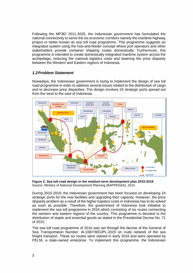
Nowadays, the Indonesian government is trying to implement the design of sea toll road programme in order to address several issues related to the distribution of cargo and to decrease price disparities. The design involves 24 strategic ports spread out from the west to the east of Indonesia.
Figure 2. Sea toll road design in the medium-term development plan 2015-2019 Source: Ministry of National Development Planning (BAPPENAS), 2015
During 2015-2019, the Indonesian government has been focused on developing 24 strategic ports for the new facilities and upgrading their capacity. However, the price disparity problem as a result of the higher logistics costs in Indonesia has to be solved as soon as possible. Therefore, the government of Indonesia took initiative to implement the sea toll programme in 2016 which consisting of six routes connecting the western and eastern regions of the country. This programme is devoted to the distribution of staple and essential goods as stated in the Presidential Decree No. 71 of 2015.
The sea toll road programme of 2016 was set through the decree of the General of Sea Transportation Number: Al.108/7/8/DJPL-2015 on route network of the sea freight transport. These six routes were started in early 2016 and were operated by PELNI, a state-owned enterprise. To implement this programme, the Indonesian

3
government provided subsidies to PELNI to operate its vessels serving the predetermined routes. The government defined the route, size of the ships, annual frequency and commission days per voyage (the number of days specified for ships sailing from the original port to the final port until returning to the port of origin). Following these six routes, the ships have limited capacity and sail to several sub-feeder ports. As a result, sometimes it takes a month for a ship to sail from its origin to the destination port and back.
In the beginning of 2017, this programme was changed by the decree of the General of Sea Transportation Number. AL.108/1/9/DJPL-17. The reason behind this change was high operational costs which consequently kept logistics costs high as well while the goal of this programme was to reduce logistics costs. There are 13 routes that are used within the sea toll road programme. Four of these routes are the result of crossing the previous routes. The network design used in the implementation of this programme is multi-port-calling which involved several calls on one route. Running this strategy in 2017, the Indonesian government also involved private companies through an open bidding process.
The Sea toll road programme of 2016 and 2017 used the concept of direct network connecting the hub port to sub-feeder ports or multi-port-calling network. The port of Tanjung Perak was appointed as one of the main ports in the western part of the country to serve as an origin port for distributing cargo to the eastern regions of Indonesia. Referring to the master plan of sea toll road programme to be implemented in 2019, the concept that should be operated is a hub-and-spoke network where the feeder port has a major role of connecting port between the hub port and the sub-feeder ports. This concept allows the use of larger sized vessels that are expected to reduce operating costs because of the ability to create economies of scale.
In line with the issues described, this research paper will analyse the efficiency in terms of the shipping costs for distributing cargo under the implementation of sea toll road programme of 2016 and 2017. This thesis will be focused on the routes starting from the Tanjung Perak port since this port has an important role of the gateway to the eastern regions of Indonesia. Furthermore, this thesis also suggests another potential route by involving the Port of Tenau Kupang as a feeder port using the hub-and-spoke network. Since the feeder port in Indonesia acts as a connecting port between the hub port and the sub-feeder port, Tenau Kupang port will have a function of a transhipment port in this study. The main idea behind this consideration is that Tenau Kupang port as one of the 24 national strategic ports involved in the master plan of the 2019 sea toll road programme. In other words, through implementation this research, it will be possible to quickly align between the current sea toll routes and the master plan of the 2019 sea toll road programme. Furthermore, as this study is in line with the National Development Planning, it may be possible to accelerate and expand the economic development in Indonesia by strengthening domestic connectivity.
1.3 Research Question
Based on the identified problem, the main research question that needs to be answered is the following:
“What is the potential impact of the port of Tenau Kupang as a transhipment port in terms of reducing shipping costs from the Port of Tanjung Perak to the South-Eastern part of Indonesia?”

4
To answer the main research question, the following sub-research questions need to be taken into account:
1. How does the implementation of container distribution from the Port of Tanjung Perak to South-Eastern part of Indonesia fit in the sea toll road programme set in 2016 and 2017?
2. How do we calculate the shipping costs of the route from the port of Tanjung Perak to the ports located in South-East of Indonesia using a multi-port calling following sea toll road programme of 2016 and 2017 and using a hub-and-spoke network that includes the Port of Tenau Kupang as a transhipment port?
3. Are the routes from the port of Tanjung Perak to South-Eastern areas of Indonesia specified in the sea toll road programme of 2016 and 2017 effective and efficient in lowering the shipping costs compared to the proposed network of involving the port of Tenau Kupang as a transhipment port?
The objective of this paper is to work out a strategy that is aimed at reducing the shipping costs on the West-East route in Indonesia. For this strategy, investigate whether it is useful to use the Port of Tenau Kupang as a transhipment port of the containers from the Port of Tanjung Perak to South-Eastern area of the country or not.
1.4 Research Topic Scope and Limitations of Research
In order to define the topic and research problem more clearly, we delimit the scope of this thesis as follows:
1. In this study, we analyse the routes defined by the Indonesian government in the sea toll road programme of 2016 and 2017, in particular all of the routes starting at the Port of Tanjung Perak. The main reason to choose this port as the port of origin for the routes to the Eastern regions of Indonesia is the fact that it serves as a gateway and distribution centre on the routes from the West to the East of Indonesia.
2. Following the master plan of sea toll road programme, Tanjung Perak port as a hub port is connected to six feeder ports i.e. Tanjung Emas, Banjarmasin, Sampit, Balikpapan, Samarinda and Tenau Kupang. In this paper, the port of Tenau Kupang is considered as a port pairing to Tanjung Perak port since this port is located in the Eastern region in Indonesia.
3. The aim of this study is to find an optimal route to minimise shipping costs of cargo distribution from the port of Tanjung Perak to South-East of Indonesia. Whether or not to involve the Tenau Kupang port as a transhipment port for the implementation of the current sea toll road programme will be the subject of this research.
4. Only containers that transport staple and essential goods are included in the analysis of this research.
5. The Indonesian government has stipulated the size of the ships, the annual frequency and the commission days per voyage (the number of days specified for ships sailing from the port of origin to the final port and back. We will follow this specification.

5
1.5 Thesis Structure
This thesis consists of five chapters.
Chapter 1 - Introduction
In this part of the study, we present an overview of the main topics that will be discussed. We also provide the main and sub-research questions.
Chapter 2 - Literature Review
This part consists of several theories to provide theoretical framework of our research. This chapter is divided into three parts. The first part is an explanation of MP3EI, design model that is used by the Indonesian government to create connectivity. In the second part, we present the description of the logistics system and the transportation system to provide an overview of the network used in this study. And in the last part, we elaborate on the theoretical framework of the total costs consists of shipping costs and the chartering concepts.
Chapter 3 - Research Methodology
In this chapter, we describe the method used in this study to work out an optimal route to minimise the shipping costs for each alternative routing. A mathematical model is developed to calculate shipping costs for each alternative route. Also, we describe the assumptions that underpin each of the three scenarios under the scheme of research methodology and data related to the methodological calculations.
Chapter 4 - Overview on the Sea Toll Road Programme in Indonesia
In this chapter, we provide a detailed description of the implementation of the sea toll road programme established in 2016 and the route changes made in 2017. Moreover, we also provide the profile of the Port of Tanjung Perak and Tenau Kupang as two main subjects in this study.
Chapter 5 - Results and Analysis
In this chapter, we answer the sub-research questions that help address the main research question of this thesis. Description of the shipping cost analysis based on three scenarios are also presented here. The first scenario reflects the condition of the sea toll road programme set in 2016, the second scenario is defined by the change to be programme made in 2017, and the third scenario includes the port of Tenau Kupang on each alternative route. At the end of this chapter, the comparison between the three scenarios is conducted in order to choose the route with the minimum shipping costs.
Chapter 6 - Conclusions and Recommendations
In this chapter, we make conclusions based on all the results of the analysis and provides recommendations that are expected to make a valuable contribution for further research and assist the Indonesian government in creating an effective and efficient route.

6
--Blank Page--

7
Chapter 2 Literature Review
In this chapter, we present theoretical framework and government regulations as the foundation of this research. Section 2.1, provides an overview of the Master Plan for the Acceleration and Expansion of Indonesia’s Economic Development (MP3EI) which is used as a reference by the Indonesian government to create the connectivity as a background to this study. The government of Indonesia requires logistics and transportation system design as a tool to realise connectivity, both locally and internationally. Hence, various theories and government regulations are discussed in Sections 2.2 and 2.3. In Section 2.4, we review the previous study conducted on this topic, to figure out how the network model works in order to minimise the total shipping costs based on the use of the mathematical model and operation research approach. Section 2.5, we present the theory on shipping costs, including operating expenses, voyage costs, and cargo handling costs and shipping charter. At the end of this chapter, we provide the description of staple goods and essential goods based on government regulation.
2.1 The Master plan for the Acceleration and Expansion of Indonesia’s Economic Development (MP3EI)
The master plan for acceleration and expansion of Indonesia’s economic development (MP3EI) is implemented to accelerate and strengthen economic development in accordance with the superiority and strategic potential of the region in six corridors (Simlitabmas, 2011). There are three main elements that are integrated as an effort to realise the MP3EI strategy.
1. Economic potential development of the region on six Indonesian Economic Corridors (EC) namely EC Sumatra, EC Java, EC Borneo, EC Sulawesi, EC Bali-Nusa and EC Papua-Maluku.
2. Strengthening domestic integration and globally connectivity. 3. Strengthening the capacity of human resources (HR) as well as national
science and technology in supporting the key programme’s development in every economic corridor (EC).
Figure 3. Six Economic Corridors in Indonesia Source: Modified from the cabinet secretariat of the Republic of Indonesia, 2014
Java EC, driver for national industry and service provision
Sulawesi EC, centre of production and processing of national agriculture, plantation, fishery, oil & gas, and mining
Kalimantan EC, centre of production and processing of national mining and energy reserves
Papua-Maluku EC, centre for development of food, fisheries, energy and national mining Sumatra EC,
centre of production and processing of national resources and as
Bali-Nusa Tenggara EC, gateway for tourism and national food support
6
6

8
Increased connectivity of the six corridors is reflected in the four elements of national policy; National Logistic System, National Transportation System, regional development and information and communication technology (The cabinet secretariat of the Republic of Indonesia, 2014). The integration of these four key elements aims to achieve national connectivity objectives that are locally integrated and globally connected. Local integration is intended to integrate the existing connectivity system effectively and efficiently to support the mobilisation of goods, services on the territory of Indonesia. In order to develop locally integrated connectivity, there should be a transport network with transport nodes. Furthermore, to support connectivity integration of communication and information is required.
Figure 4. National Connectivity Framework Source: modified from the cabinet secretariat of the Republic of Indonesia, 2014
In line with the MP3EI, the Indonesian government issued the blueprint of national logistic system development and national transportation system.
2.2 National Logistics System
The logistics system handles all the activities related to the delivery of goods or products from origin to destination. Origin point acts as a manufacturer because it serves as a supplier of goods, both as a producer and a distributor, and the destination point works as a consumer, either directly or indirectly.
Logistics management has a vital role in supporting the economy and prosperity of a country. Good logistics management helps the businesses to be competitive through cost efficiency which generates more value for the product or service. Furthermore, increasing competitiveness leads to improving the welfare of the community. In this regard, the World Bank has a special perspective on the logistics sector, with an emphasis on the costs and improvements to the quality of logistics and transportation systems that increase access to international markets, and thereby directly impact trade and income increment and can significantly reduce poverty. The World Bank is periodically conducting a survey of Logistics Performance Index (LPI) across 160 countries in the world. Logistics Performance Index is an assessment tool used to help countries identify the challenges and opportunities they face in logistics performance and is expected to improve their performance (World Bank, 2016).
Regional Development
ICT National
Transportation System
National Logistics System
Connectivity
Locally integrated,
Globally connected
9
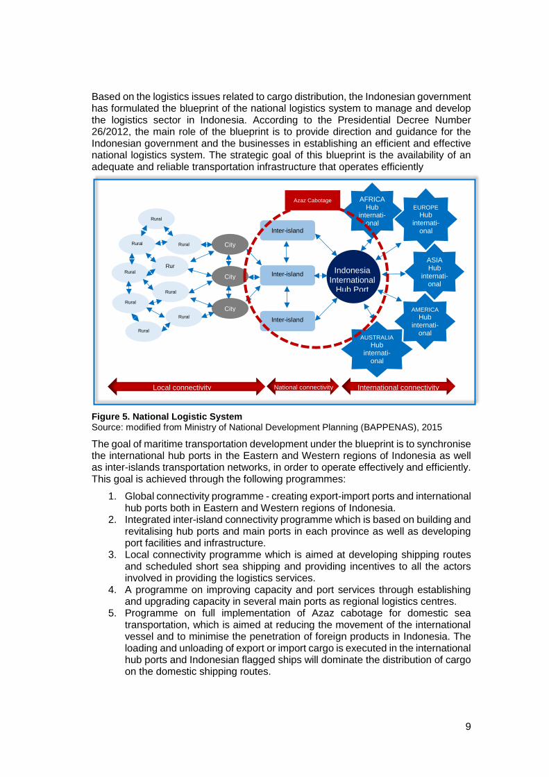
Based on the logistics issues related to cargo distribution, the Indonesian government has formulated the blueprint of the national logistics system to manage and develop the logistics sector in Indonesia. According to the Presidential Decree Number 26/2012, the main role of the blueprint is to provide direction and guidance for the Indonesian government and the businesses in establishing an efficient and effective national logistics system. The strategic goal of this blueprint is the availability of an adequate and reliable transportation infrastructure that operates efficiently
Figure 5. National Logistic System Source: modified from Ministry of National Development Planning (BAPPENAS), 2015
The goal of maritime transportation development under the blueprint is to synchronise the international hub ports in the Eastern and Western regions of Indonesia as well as inter-islands transportation networks, in order to operate effectively and efficiently. This goal is achieved through the following programmes:
1. Global connectivity programme - creating export-import ports and international hub ports both in Eastern and Western regions of Indonesia.
2. Integrated inter-island connectivity programme which is based on building and revitalising hub ports and main ports in each province as well as developing port facilities and infrastructure.
3. Local connectivity programme which is aimed at developing shipping routes and scheduled short sea shipping and providing incentives to all the actors involved in providing the logistics services.
4. A programme on improving capacity and port services through establishing and upgrading capacity in several main ports as regional logistics centres.
5. Programme on full implementation of Azaz cabotage for domestic sea transportation, which is aimed at reducing the movement of the international vessel and to minimise the penetration of foreign products in Indonesia. The loading and unloading of export or import cargo is executed in the international hub ports and Indonesian flagged ships will dominate the distribution of cargo on the domestic shipping routes.
AUSTRALIA
Hub internati-
onal
AFRICA Hub
internati-onal
Inter-island
Inter-island
Inter-island
Rural
Rural
Rural
Rural
Rural
Rural
Rural
Rural
Rural
City
City
City
Indonesia
International Hub Port
EUROPE
Hub internati-
onal
ASIA Hub
internati-onal
AMERICA
Hub internati-
onal
Local connectivity National connectivity International connectivity
Azaz Cabotage

10
6. Programme on improving accessibility of sea freight in the underdeveloped and remote regions by optimising pioneering services, including short-sea shipping and encouraging the use of Ro-Ro vessels.
7. Programme on improving the number of fleets by developing domestic vessels
2.3 Transportation System
Transportation has an important role in the design of logistics system. The existence of a good transportation system has an impact on improving the logistics system. In addition, a good transportation system in logistics activities allows for increasing efficiency, reducing operating costs, and improving service quality. Improving the transportation system requires both public and private sectors. The support of a good transportation system in the logistics system will enhance the competitiveness of government and the companies. In Section 2.3.1, we discuss the differences between multi-port calling and hub-and-spoke network. Section 2.3.2 provides an analysis of the hub-and-feeder network in Indonesia under the Master Plan Sea Toll Road Programme that will be implemented in 2019.
2.3.1 Hub-and-Spoke vs. Multi-Port-Calling Network
Ronen (1983, 1993) and Christiansen, et al. (2004) stated that there are two main types of research in shipping service network design problem i.e. tramp shipping service network and liner shipping service network. Tramp shipping network deals with ship routing and vessels deployment for delivering bulk cargo without considering the H&S network operation. Because of this type of network, the cargo volume between the origin and the destination port is very big, and, therefore, cargo consolidation is not necessary on the hub port. The current studies on liner shipping service network can be classified into two categories – with and without the role of the hub port as a place where cargo is consolidated. In other words, there are two different design network alternatives on shipping liner network, namely Hub-and-Spoke (H&S) and Multi-Port-Calling (MPC).
Imai, et al. (2006) noted an interesting phenomenon - rapid growth in ship size leads to changes in the service network from multi-port-calling to the hub-and-spoke network. Over the past few years, there has been an unprecedented increase in the number of container ships serving the world's most densely packed maritime routes. This can be attributed to the fact that a more flexible and widespread form of cooperation has emerged in the maritime industry, 'The global alliances', which are so dominant on the main routes, have proven to be very successful in gaining the economies of scale achieved through the use of larger vessels. The hub-and-spoke (H&S) network entails using a mega-containership and the multi-port-calling system (MPC) is operated using smaller containerships (Imai, et al., 2009).

11
Figure 6. Service networks Source: Imai, et al., 2009
A port might have a function of a regional port for one liner shipping operator or a function of a feeder port for another one (Notteboom & Rodrigue, 2008). Driven by economic factors, the port developed into two port types namely the hub port that serves the mother vessels, and the secondary port or commonly called the port 'spoke' (Mourao, et al., 2002). When the hub and spoke system was created, the feeder or land transportation mode moved the cargo to and from the hub port and used the port to consolidation transport flows. The low volume of goods transported between certain ports and the high fixed costs incurred by the vessels encouraged more intense use of this hub and spoke system (Mourao, et al., 2002). Mulder & Dekker (2014) made a distinction between the main services and the feeder services. The feeder services are used to ship the cargo from the cluster centre in one cluster to the other ports in the same cluster.
A hub-and-spoke network is a network pattern that has one or more ports that serve as a hub port in the destination area based on the geographical location and demand for shipping items (Hsu & Hsieh, 2007). Major ports are frequently selected as hub ports, and the other ports act as feeder ports or spoke ports. The cargo transported is consolidated at the port hub and then delivered by the larger vessels that provide inter-hub port services in both areas. Meanwhile, to provide services between port hubs and small ports small vessels (feeder vessels) are used. Figure 7 illustrates the fundamental hub-and-spoke maritime network. In their study, Hsu & Hsieh (2007) explained that each region has one or more hub ports (p3, p4, p5 and p6) and other ports act as feeder ports (p1 and p2). A container can be shipped directly from a feeder port in the region of origin to a hub port in the region of destination directly or have it transported through the hub port at the region of origin by routing the feeder line and then the main line.

12
Figure 7. The fundamental hub and spoke maritime network Source: Hsu & Hsieh, 2007
The connection between hub port and feeder port could use direct feeder shipping or a shuttle feeder services consisting of one feeder port or indirect feeder ships using a cyclic line bundling service that contains more than one feeder port (Polat, et al., 2014). The direct feeder shipping has an advantage in having the lowest transit time but requires smaller feeder containerships. In contrast, cycling feeder services offer the benefit of economies of scale but take a longer distance and subsequently generate longer transit times.
Figure 8. Feeder service network as a part of H&S network Source: Polat, et al., 2014
13
Meng & Wang (2011) offer perspectives related to the network system changes from the MPC network to a combined H&S and MPC network resulting from increased ship size and shipment demand. The combined H&S and MPC network has characteristics of a conventional H&S network, larger vessels operate in the main line and feeder vessels serve the feeder line. The H&S network is used when container volume is not enough to justify a direct network, and thus, some containers have to be transhipped at hub ports.
2.3.2 Hub-and-Feeder Network in Indonesia
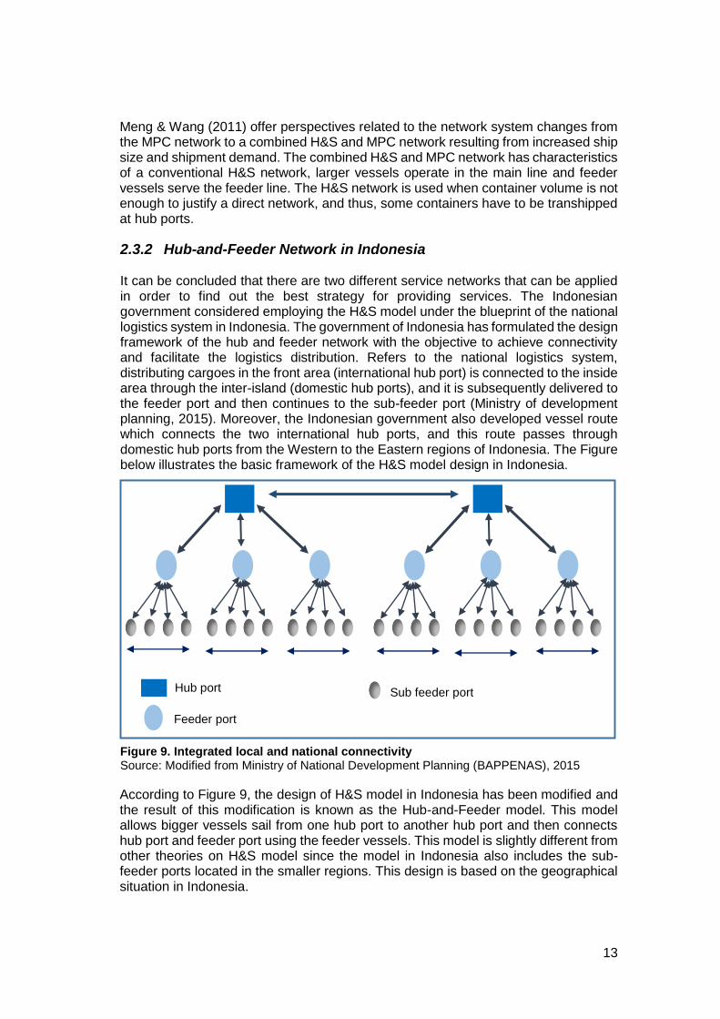
It can be concluded that there are two different service networks that can be applied in order to find out the best strategy for providing services. The Indonesian government considered employing the H&S model under the blueprint of the national logistics system in Indonesia. The government of Indonesia has formulated the design framework of the hub and feeder network with the objective to achieve connectivity and facilitate the logistics distribution. Refers to the national logistics system, distributing cargoes in the front area (international hub port) is connected to the inside area through the inter-island (domestic hub ports), and it is subsequently delivered to the feeder port and then continues to the sub-feeder port (Ministry of development planning, 2015). Moreover, the Indonesian government also developed vessel route which connects the two international hub ports, and this route passes through domestic hub ports from the Western to the Eastern regions of Indonesia. The Figure below illustrates the basic framework of the H&S model design in Indonesia.
Figure 9. Integrated local and national connectivity Source: Modified from Ministry of National Development Planning (BAPPENAS), 2015
According to Figure 9, the design of H&S model in Indonesia has been modified and the result of this modification is known as the Hub-and-Feeder model. This model allows bigger vessels sail from one hub port to another hub port and then connects hub port and feeder port using the feeder vessels. This model is slightly different from other theories on H&S model since the model in Indonesia also includes the sub-feeder ports located in the smaller regions. This design is based on the geographical situation in Indonesia.
Hub port Sub feeder port
Feeder port

14
2.4 Network Model
In this section we discuss previous studies conducted in this field, particularly, studies on the optimisation of the liner shipping routes. Review of previous studies is essential to figure out how the network model works in order to optimise the network with the help of the mathematical model and operation research approach. We consider to review these previous studies in this research paper since these are pre-reviewed and have been cited by a lot of others researchers. In Section 2.4.1, several references with respect to the optimal shipping routes creation are presented. The construction of MPC and H&S network are the main topics of discussion in Section 2.4.2. Theory related to pendulum service is introduced in Section 2.4.3.
2.4.1 Optimisation Method in Linear Network Design Problem
Mulder & Dekker (2014) have conducted the study using aggregation methods to solve the combined fleet-design, ship scheduling and cargo routing problems when looking at the limited capacity of ships in liner shipping. First, the ports are aggregated into port clusters in order to solve the problem of size. Initial route is developed and a linear programming formulation which is known as cargo routing problem is constructed to solve the cargo routing problem to be optimal. Second, they had to disaggregate again into individual ports after the results in clustered port were obtained. A distinction between main services and feeder services are introduced in their research. The feeder services are used to move the cargo from the centre of the cluster to the other ports in the cluster. Moreover, the centre of the cluster can be a part of main services and the other ports will be added to the main services network only if it is profitable. In this method, only intra-regional demand is taken into account. In their study, however, there is a possibility to add regional demand in the model, as the method will stay the same when regional demand is included. Finally, they developed ten scenarios with undertrained demand and compared them to the performance of the reference network and its profit levels.
Wardana (2014) developed two methods; Travelling Salesman Problem (TSP) and heuristics approach to create a service network for liner shipping in Indonesia. This research was conducted to study what impact the selected routes have on cargo allocation. The author used the nearest neighbouring algorithm as a solution method for the TSP model, to find out the fastest path in determining the next destination port after visiting the previous port. The heuristics approach was used to decide cargo allocation and to try to generate the highest profit levels from the selected routes. Profit generated by reducing the revenue and the costs. The author created the possible routes based on demand. The simulation of all possible routes that combined ship routing and cargo allocation was executed with the help of the Excel spreadsheet.
Van Rijn (2015) examined the design of a service network for liner shipping in Indonesia. This study constructs service networks consisting of different shipping routes, ship allocations, sailing speeds and cargo volume allocations. Two algorithms were developed in order to formulate the service network. The first algorithm used pendulum routes, and the second algorithm used randomly generated routes. The routes used in the route network of this study is based on the routes proposed by the Indonesian government.

15
Lazuardi (2015) analysed the connectivity between main port and international hub port in Indonesia. This study applied a heuristic approach combined with the use of the Feeder Network Design Problem (FNDP) and Multiple Commodities Problem in order to create the optimal route and cargo allocation by minimising the total transportation costs. There were two scenarios in this study, the first scenario analysed all the international containers of six main domestic ports, including Belawan, and the second scenario did not include the international container in Belawan. As a result of this study, two optimal routes for each scenario was suggested, consisting of a direct and indirect loop. The direct loop was defined as a direct connection between the hub and main domestic ports, while the indirect loop meant calling at multiple main domestic ports.
2.4.2 Construction of MPC and H&S Network in liner shipping network
Imai, et al. (2006) studied mega container vessels’ viability by using a game theory model in competitive circumstances. In order to simplify the model, this study permitted each shipping company to have only two strategies, either by using mega container vessels or – alternatively – using smaller vessels. Service network structures in liner shipping routes were developed, then this study assumed that only two service networks were allowed: the hub-and-spoke (H&S) network for mega container vessels and multi-port-calling (MPC) for smaller vessels. The construction of H&S and MPC networks was chosen to minimise of origin and destination (O-D) traffic travel length weighted by shipment volumes. To make computations easier, the MPC network was constructed as “the travelling salesman” problem, while the H&S network was identified as “the minimum location” problem.
Hsu & Hsieh (2007) have formulated a two-objective optimisation model by minimising shipping costs and inventory costs to determine the optimal liner shipping routes, the size of vessels and sailing frequencies for container lines. Shipping costs can be distinguished into three categories; capital and operating costs, fuel costs and port charges. Inventory costs are associated with traffic volumes, the value of the cargo, and storage time length. In this study, only inventory cost related to shipping processes are considered and so are involving the waiting time and costs of shipping time. Firstly, this study uses an analytical method to formulate shipping and inventory costs. Then, Pareto optimal solutions are used to determine the two-objective model based on a trade-off between shipping and inventory costs. A fundamental hub-and-spoke network is taken into account in this study. Therefore, the objective optimisation model is not only used to determine optimal ship size and sailing frequencies but also decision-making processes on different scenarios of shipping routes.
Imai, et al. (2009) have examined two different alternatives of service networks for liner shipping routes, namely a multi-port-calling (MPC) network for conventional ship sizes (smaller ships) and a hub-and-spoke model for mega container ships. This study was conducted to refine the research that has been done before, where the design of liner shipping networks is taking into account container management problems including empty container repositioning. Two phases are performed to create a solution process, namely the service network design and container distribution. This research studies the MPC network as the minimisation of the total origin-destination traffic travel length weighted by the shipment volume by using a genetic algorithm (GA)-based heuristic. The MPC network does not consider a ship’s capacity overutilization since it is not associated with fluctuations in demand. Also, the ship is

16
not based on a specific port, therefore the carried cargoes are delivered to the ports in any calling sequence. The MPC construction is given as follows: set up the ports to be called and carried a number of the containers between the ports of origin and destination ports. This model has similar characteristics to the travelling salesman problem where one round route starting from an origin port and returning to this port after visiting all the ports with only one call. While the outline of the H&S network is constructed differently: there are two sets of calling ports and a number of containers is carried between the origin and destination ports. This model takes into account the existence of the hub ports and each feeder port in a region.
Meng & Wang (2011) conducted research to propose a medium-term liner shipping network design problem, referred to as a liner shipping service network, combining the H&S and MPC network operations and also empty container repositioning. The combination of H&S and MPC networks in liner shipping service networks has two main characteristics: 1) Container transhipment costs and handling times cannot be ignored because these costs are a substantial part of the operating costs; 2) Allowing the direct container shipment between any two ports including feeder ports. These two unique characteristics means that the combined H&S and MPC networks are significantly different from the conventional H&S operations networks.
2.4.3 Pendulum Network
According to Notteboom (2004), pendulum services are commonly used on the main east-west trading routes. The pendulum service relies on a hub port that serves as a turning point between the liner services of two different trades and is serviced by post-panamax vessels. The design of this kind of liner service has become popular in the high-volume international trade routes such as the US West coast-Far East- Europe trade. Consequently, in the last decade a new generation of loading centres along the east-west shipping lanes has been developed. These sites depend heavily on the flow of traffic generated by the interaction of places that are widely separated and stimulated by port location.
The pendulum service involves a regular schedule between port sequences that frequently serves by geographical proximity. Several ports along one coastal area are serviced and this process is repeated regularly (Lun & Browne, 2009). Chen & Zeng (2010) argued that container shipping networks can be distinguished into two types depending on their operating characteristics. The first is circular and the other is pendulum as shown in Figure 10. According to the Figure below, any pendulum route can be changed into a circular route as a basic form by inserting virtual port(s) in the backward direction and developing an adequate matrix for demand distributions.

17
Figure 10. a) Pendulum route; b) Circular route
Source: Chen & Zeng, 2010
We can deduce that this study requires an analytical approach that probably combines with two or more methods to generate optimal solutions by minimising shipping costs. In this research, we develop two liner shipping network designs: the multi-port-calling (MPC) one, combined with pendulum services as followed by the sea toll road programme of 2016 and 2017 as stipulated by the Indonesian government. The other is the Hub-and-Spoke as a proposed network including the port of Tenau Kupang as a transhipment port. The result of these two networks will be compared in order to determine the optimal route that generates the lowest cost.
2.5 Transportation Costs
The ability of ship operations in terms of cargo distribution will affect the profitability and quality. Factors affecting operational performance include scheduling, ship routing, and ship size. Using larger vessels allows lower shipping costs per container as a result of economies of scale. In addition, the speed of the vessel and the productivity of loading and unloading containers is also a determinant of the costs to be incurred by the vessel.
2.5.1 Shipping Cost
In general, there are three basics factors combined in running a vessel. First, the cost of fuel consumption, the number of crew needed, and the condition of the vessel that is an indication for repair and maintenance requirements. Then, the cost of the purchase order, bunkers, wages, repairing costs and the interest rate. Third, administration costs and operational efficiency.

18
Stopford (2009) classifies shipping costs into five categories as follows:
1. Capital costs These costs depend on the way the ship has been financed (the form of equity or debt finance). In other word, capital costs include the cost calculation covering interest payments and returning the dividend depends on how the ship has been financed.
2. Operating costs Operating costs consist of the expenses related to the day-to-day running of the vessel and day-to-day repairs and maintenance (not major dry docking).
a. Crew costs Crew costs or manning costs including basic salaries and wages, insurance, pensions, repatriation and victuals expenses. Manning costs depend on the size of the crew employed and employment policy adopted by the owner based on the ship’s flag state.
b. Stores and consumable These costs are categorised into two different items; general stores, including cabin stores and various items used on-board of the ships as well as lubricating oils as major costs.
c. Repairs and maintenance Repair costs cover the standard requirement to maintain the vessel based on a company policy. While the maintenance costs cover the routine maintenance, including breakdowns and spares.
d. Insurance Two-thirds of these costs cover the hull and machinery that insure the owner of the vessel from the physical loss or damage, and the other part covers the third party insurance which concerns the third party liability such as collision, cargo damage, death of crew, pollution, and other matters that can be covered in the open insurance market.
e. General costs General costs include administrative and management charges, miscellaneous costs, owners’ port charges and communication fees.
3. Periodic maintenance costs These costs include the cost of docking and special surveys. The cost level depends on the age and the condition of the ship. In order to maintain its seaworthiness, a ship shall be docking every two years, while the special survey should be conducted every four years.
4. Voyage costs These costs are built up of three basic variable costs that occur in a particular voyage, i.e. fuel costs, port charges and canal fees.
1. Fuel costs Fuel consumption depends on the ship design, ship age, the design of the main and auxiliary engines, and hull condition as well as the speed level at which the ship is operated. Operation of the vessel at lower speed leads to fuel savings.

19
2. Port charges These costs can be divided into two categories: port dues and service charges. Port dues are charged to the vessel for general use of the port infrastructure, such as line handling fees, berth occupancy charges, wharf age charges and other provisions related to the basic port infrastructure. While, service charges including pilotage, tugging and cargo handling will be more discussed in the next section.
Port charges can be categorised into the shipping charges and stevedoring charges. The shipping charges consist of pilotage, towage, and anchoring fees as well as berth occupancy charges. While, stevedore charge including loading and unloading fees, the use of equipment and stacking cost in the container yard (Hsu & Hsieh, 2007).
3. Canal fee Canal fees are paid on the use of a canal, where there are two canals in the world namely the Suez and Panama Canals. Because in this study we focus on discussing shipping costs in Indonesia, the canal fee element can safely be ignored.
5. Cargo-handling costs Cargo-handling costs consist of loading and discharging costs. These costs are a significant component in the total shipping cost. In general, the type of this cost depends on the type and size of the containers, whether they are empty or full and whether they are20’ or 40’ feet.
In order to make more detail, the shipping costs have been identified and linked as is shown in Figure 11.
Figure 11. Shipping cash flow model Source: Modified from Maritime Economics, third edition, Martin Stopford, 2009, p. 220

20
In this study, we decide to use the time charter method. As mentioned in the previous section, the ship-owner is obliged to pay all of the expenses related to the operational and capital costs excluding fuel costs, port dues and cargo handling fees. Therefore, the calculation of the shipping costs in this study is the sum of the operating costs based on the time charter rate, fuel consumption costs, port dues and cargo-handling fees.
2.5.2 Shipping Charter
Shipping companies might use their vessels or charter vessels in serving cargo distribution. According to Stopford (2009), there are three types of charter vessels that are commonly used; bareboat charters, time charters and voyage charters:
1. Bareboat charter A bareboat charter is an arrangement for chartering a ship where the charterer pays all the operating costs, voyage costs and costs related to cargo. Moreover, the charterer also takes both the operational and market risks.
2. Time charter A time charter is an arrangement for hiring a ship at a specified rate with a fixed daily or monthly payment. The ship-owner takes an operational risk in case the ship breaks down. While, the charterer takes a risk in terms of shipping market risk, the agreed rate must be paid regardless of market conditions. Moreover, the charterer pays fuel costs, port dues and port charges, stevedoring and other costs related to the cargo.
3. Voyage charter Under this arrangement, the ship-owner has an obligation to pay all the expenses excluding cargo handling and also is liable for operating the vessel including the planning and execution of the voyage. In this scheme, the ship-owner takes the operational and market risks. In other words, when there is no cargo, the ship breaks down or the vessel has to wait for cargo, the ship-owner will face losses.
In Table 1, we represent the division of expenses for different vessel hiring contracts
Remark Voyage Charter
Time Charter Bareboat Charter
Voyage Expenses Ship-owner Charterer Charterer Operational Expenses Ship-owner Ship-owner Charterer Capital Expenses Ship-owner Ship-owner Ship-owner
Table 1. Division of expenses for different vessel hire contracts Source: Lecture of Ship Finance by Pruyn, 2016
2.6 Staple and Essential Goods
According to Business Dictionary (2017), staple goods are “consumer goods (such as bread, milk, paper, sugar) that are bought often and consumed routinely”, while “some essential good types that are produced by business operators include food, water, gasoline and heating fuel, as well as residential building materials that can be used to construct homes for shelter”.

21
Sea toll road programme 2016 and 2017 are devoted to the distribution of staple and essential goods as stated in Presidential Decree No. 71 of 2015 on the stipulation and storage of staple and essential goods. In pursuance of this regulation, staple and essential goods consist of:
1. Staple goods
a. Agricultural products 1) Rice 2) Soybeans 3) Chili 4) Shallot
b. Industrial products 1) Sugar 2) Cooking oil 3) Wheat flour
c. Livestock and fishery products 1) Beef 2) Chicken meat 3) Chicken eggs 4) Fish
2. Essential goods
a. Seeds are rice seed, corn, and soybean b. Fertiliser c. Heating fuel d. Plywood e. Cement f. Light steel

22
--Blank Page--

23
Chapter 3 Research Methodology
A fundamental hub-and-spoke and a multi-port-calling network are taken into account in this study. Container shipping services are provided by the carrier between two regions separated by the ocean. Since the design of the hub-and-spoke model in Indonesia is slightly different from the common model introduced by several researchers in earlier work, we adapted the model by involving sub-feeder ports as part of the hub-and-spoke network. If the distribution of goods is conducted from hub to hub and then will be distributed to the feeder port, in this study we will analyse the distribution of goods from the hub port to the feeder port and then to the sub-feeder port. In that case the function of the feeder port in this study is one of a transhipment port. In section 3.1, a mathematical model for shipping cost functions is defined. Shipping costs consist of operating costs that are based on time charter rates, fuel consumption costs, port dues and cargo-handling fees on the route being served. Section 3.1.1 further determines shipping cost functions for multi-port-calling networks, followed by the hub-and-spoke network in section 3.1.2. The assumptions are explained in section 3.2 and followed by the research methodology scheme presented in this study in section 3.3. The last section will present the relevant data that is required in this study.
3.1 Shipping cost function
Based on Stopford (2009), shipping costs can be calculated as a sum of capital costs, operating costs, periodic maintenance costs, voyage costs and cargo handling costs. In this research, we consider that the ship is hired by using a time charter arrangement with the charter rate in Dollar per day (US$/day). Further, we change capital costs, operating costs and periodic maintenance costs by applying the time charter rate in unit dollars per day (US$/day), thus shipping costs is a sum of time charter rate, fuel costs, port dues and cargo handling costs as shown in the following formula:
𝐶𝑆𝑚 = ∑ [𝛼𝑖𝑡 + 𝑂𝑡𝑊𝑖 + 𝐹𝑖𝑡 + 𝐷𝑖
𝑚 (𝑂𝑡
𝑉𝑡+
𝐹𝑡
𝑉𝑡)] + ∑ ∑ [(𝛽𝑖 +
𝑂𝑡
𝑅𝑖) 𝑃𝑖𝑗]
𝑗𝑖
𝑖
Subject to
𝛼𝑖𝑡 = ∑ 𝑃𝑙𝑖𝑡 + 𝑇𝑜𝑖𝑡
𝑖
+ 𝐿𝑖𝑡 + 𝐵𝑖𝑡
Where:
m route i port of origin on route m j port of destination on route m t type of ship 𝛼𝑖𝑡 fixed portion of port i charge for a ship of type t (US$) 𝑂𝑡 average daily charter rate for a ship of type t (US$/day) 𝑊𝑖 time a ship spends on the arrival and departure process in port i (day)
𝐹𝑖𝑡 fuel cost in port i by a ship of type t (US$) 𝐷𝑖
𝑚 shipping distance between port i and port i + 1 on route m (nautical mile)
[1]

24
𝑉𝑡 service speed for a ship of type t (knot)
𝐹𝑡 fuel cost at sea for a ship of type t (US$) 𝛽𝑖 average handling fee per TEU in port i (US$ per TEU) 𝑅𝑖 average gross handling rate in port i (TEU per day)
𝑃𝑖𝑗 the number of containers shipped between port i and port j on route m (TEU)
𝑃𝑙𝑖𝑡 pilotage for a ship of type t (US$) 𝑇𝑜𝑖𝑡 towage for a ship of type t (US$)
𝐿𝑖𝑡 anchoring fee for a ship of type t (US$)
𝐵𝑖𝑡 berth occupancy charge for a ship of type t (US$)
𝐺𝑖 loading and unloading fee (US$/box)
The objective of the proposed model is to minimise shipping costs. The fixed
component (Λ𝑡𝑚) and the variable shipping cost (𝜙𝑡
𝑚) for ship type t on route m can
further be denoted by simplifying the variables as:
Λ𝑡𝑚 = ∑ [𝛼𝑖𝑡 + 𝑂𝑡𝑊𝑖 + 𝐹𝑖𝑡 + 𝐷𝑖
𝑚 (𝑂𝑡
𝑉𝑡+
𝐹𝑡
𝑉𝑡)]
𝑖
𝜙𝑡𝑚 = ∑ ∑ [(𝐺𝑖 +
𝛽𝑖𝑡
𝑅𝑖+
𝑂𝑡
𝑅𝑖) 𝑃𝑖𝑗]
𝑗𝑖
Furthermore, the shipping cost equation can be simplified as
𝐶𝑆𝑚 = Λ𝑡
𝑚+ 𝜙𝑡
𝑚
The shipping cost function as denoted in equation [1] and simplified in equation [4] is a basic formula to calculate the total shipping costs in our excel sheet. Moreover, we use unit cost (Cij) as the variable cost of one unit container (TEU). Unit cost for every
route within arc (i, j) derived by dividing the total variable shipping cost (𝜙𝑡𝑚) by the
number of containers carried from origin to destination (Pij). While, the fixed cost (Λ𝑡𝑚)
dependent on the type of ship and route (Xij). Hence, we formulate the objective function [3] to determine the minimum shipping costs of distributing cargo on a certain route, as follows:
𝑀𝑖𝑛 ∑ ∑ ∑[𝑃𝑖𝑗 ∗ 𝐶𝑖𝑗]
𝑑∈𝐷𝑐∈𝐶𝑖,𝑗∈𝑁
+ ∑ Λ𝑡𝑚
𝑖,𝑗∈𝑁
∗ 𝑋𝑖𝑗
3.1.1 Shipping Cost Functions for Multi-Port-Calling Network
In order to figure out the total shipping cost for a multi-port-calling network, we construct the formula that refers to equation [4] and substitutes the number of sailing frequencies on a certain route (f) per year.
𝐶𝑆𝑑 = Λ𝑡
𝑚+ 𝜙𝑡
𝑚
= f Λ𝑡𝑚 + 𝜙𝑡
𝑚
= 𝑓 ∑ [𝛼𝑖𝑡 + 𝑂𝑡𝑊𝑖 + 𝐹𝑖𝑡 + 𝐷𝑖𝑚 (
𝑂𝑡
𝑉𝑡+
𝐹𝑡
𝑉𝑡)] + ∑ ∑ [(𝛽𝑖 +
𝑂𝑡
𝑅𝑖) 𝑃𝑖𝑗]𝑗∈𝑁𝑖∈𝑁 𝑖∈𝑁
The objective function refers to equation [3] and substitute the number of sailing frequency (f), subject to:
[4]
[6]
[7]
[5]
[3]
[2]

25
Connectivity constraint
𝑋𝑖𝑗 ∈ {0,1}
∑ 𝑋𝑖𝑗 ≥ 1 ∀ 𝑗 ∈ 𝑁
𝑖∈𝑁
∑ 𝑋𝑖𝑗 ≥ 1 ∀ 𝑖 ∈ 𝑁
𝑗∈𝑁
Cargo allocation constraint:
∑ 𝑃𝑖𝑗 = 𝐷𝑗 ∀ 𝑗 ∈ 𝑁
𝑖∈𝑁
∑ 𝑃𝑖𝑗 = 𝑆𝑖 ∀ 𝑖 ∈ 𝑁
𝑗∈𝑁
𝑃𝑖𝑗 ≥ 0 𝑎𝑛𝑑 𝑖𝑛𝑡𝑒𝑔𝑒𝑟 ∀ 𝑖, 𝑗 ∈ 𝑁
Ship capacity constraint
∑ 𝑃𝑖𝑗 ≤ ∑ 𝑈𝑡𝑋𝑖𝑗
𝑡∈𝑇𝑖,𝑗 ∈𝑁
Where:
𝑋𝑖𝑗 binary variable 1 = if ship sails from port i to port j using ship of type t 0 = otherwise N all nodes on route m
𝐷𝑗 total demand of the container (TEU) at port j
𝑆𝑖 total supply of the container (TEU) from port i
𝑈𝑡 maximum TEU capacity of ship type t per voyage
We construct three constraints in order to gain the objective of this study. Firstly, we develop connectivity constraint, equation [8] depicts that ship sails from port i to port j (1) or not (0). Equations [9] and [10] indicate that the sum of travelling routes should be equal or more than 1, since this multi-port-calling model is used to capture the shipping costs in the implementation of the sea toll road programme of 2016 and 2017 where a vessel is allowed to visit port more than once in one route (pendulum service).
Due to the fact that the number of the container discharged at destination ports are from the port of Tanjung Perak as a port of origin, we formulate the equation [11] that illustrates that the number of containers discharged at the destination port should be equal to the total demand in this port. The similar way is applied to equation [12], the total number of containers loaded at the port of origin should be equal to the total supply in this port. The last constraint of cargo allocation is shown in equation [13], where the number of containers should be equal or more than zero and must be an integer. It means that the number of containers should have a positive value.
Ship capacity constraint delineates that the number of containers carried from the port of origin to the destination port should be less than or equal to the maximum ship capacity (TEU).
[8]
[13]
[14]
[9]
[10]
[11]
[12]

26
3.1.2 Shipping Cost Function for Hub-and-Spoke Network
In order to formulate the hub-and-spoke network, we consider combining the costs in two lines, i.e. main line (h) and feeder line (s). Moreover, the minimum shipping costs are derived from the minimum sailing frequency, indicating the use of the bigger vessel capacity. Since the number of containers carried on a ship cannot exceed its capacity on any route, the sailing frequency must be equal to the maximum network flow (Maxk). The minimum sailing frequency (f) can be formulated as:
𝑓 = 𝑓𝑡ℎ−𝑚𝑖𝑛 =
𝑚𝑎𝑥𝑘 ∑ ∑ 𝛿𝑖𝑗𝑘
ℎ 𝑄𝑖𝑗ℎ
𝑗𝑖
𝑈𝑡
Where:
𝑓𝑡ℎ−𝑚𝑖𝑛 the minimum sailing frequency w.r.t. to a ship type t on the main line
𝑚𝑎𝑥𝑘 maximum network flow
𝛿𝑖𝑗𝑘ℎ the binary variable
𝛿𝑖𝑗𝑘ℎ =1, if route from port i to j contains a link between port k and k+1
𝛿𝑖𝑗𝑘ℎ =0, otherwise
𝑄𝑖𝑗ℎ Flow from port i to j on the main line per season (TEU)
𝑈𝑡 Ship’s capacity (TEU) given by the Indonesian government
Then the minimum shipping cost on the main line can be represented as 𝐶𝑆,𝑡ℎ .
Substituting formula [15] into formula [4] leads to the following equation
𝐶𝑆,𝑡ℎ =
𝑚𝑎𝑥𝑘 ∑ ∑ 𝛿𝑖𝑗𝑘
ℎ 𝑄𝑖𝑗ℎ
𝑗𝑖
𝑈𝑡 Λ𝑡
𝑚 + 𝜙𝑡𝑚
=𝑚𝑎𝑥
𝑘 ∑ ∑ 𝛿𝑖𝑗𝑘ℎ 𝑄𝑖𝑗
ℎ𝑗𝑖
𝑈𝑡∑ [𝛼𝑖𝑡 + 𝑂𝑡𝑊𝑖 + 𝐹𝑖𝑡 + 𝐷𝑖
𝑚 (𝑂𝑡
𝑉𝑡+
𝐹𝑡
𝑉𝑡)] +𝑖∈𝑁
∑ ∑ [(𝛽𝑖 +𝑂𝑡
𝑅𝑖) 𝑃𝑖𝑗]𝑗∈𝑁𝑖∈𝑁
We denote total shipping costs as TCs of the main line (h) and feeder line (s).
𝑇𝐶𝑠 = 𝐶𝑆,𝑡ℎ + 𝐶𝑆,𝑡
𝑠
3.2 Assumption
In this section, we introduce several assumptions used in this research to simplify the calculation and derive the goal of this study. These assumptions can be explained as follows:
1. The demand and supply come from 16 domestic ports based on the average total container loading and unloading for each port over the last five years. The ports that are involved in the sea toll road programme of 2016 and 2017 include such ports as Tanjung Perak, Wanci, Namlea, Fak-Fak, Kaimana, Timika, Kalabahi, Saumlaki, Moa, Dobo, Merauke, Larantuka, Loweloba, Sabu, Rote and Waingapu.
[15]
[16]
[17]

27
2. We assume that demand and supply at the port of Moa and Sabu is equal to the port of Saumlaki since the total population is relatively the same. The reason behind this consideration is that these ports are small-scale ports and are not commercially operated. Before implementing the Sea Toll Road Programme of 2016, only passenger vessels and RoRo vessels came to these ports. Therefore, the report on the number of containers from Tanjung Perak to these ports and back do not capture this data.
3. The port of Tenau Kupang is proposed to be a transhipment port that can handle the total number of containers from the Port of Tanjung Perak before being deployed to the destination ports.
4. We assume that the terminal handling cost in non-commercial ports is equal to the nearest commercial port using the ship gear. Because there is no terminal operator that provides loading and unloading activities, several ports were identified as non-commercial ports (Dobo, Kaimana, Larantuka, Lewoleba, Moa, Namlea, Rote, Sabu, Saumlaki, Timika and Wanci). For these ports, the activities are directly handled by workers in the port under the supervision of the local port authority.
5. We consider using time charter vessels with the daily charter rate in Dollar per day (US$/day) to cover the capital costs, operating costs and periodic maintenance costs. Hence, shipping costs in this study is a sum of time charter rate, fuel costs, port dues and cargo handling costs.
6. The total shipping time per round voyage is a sum of the total time spent at sea and at the port. The total time at sea is based on the distance between the ports and the speed used. The total time at the port depends on the idle time and the time spent for container handling. The latter is based on handling productivity (TEU per day). In order to calculate the idle time at the port, we use the set target waiting times based on the port classification.
7. This study only takes into account the containers that carry staple and essential goods. We use the percentage based on Tanjung Perak report in order to capture the number of containers that contains this type of goods. The percentage derived by dividing the number of staple and essential goods by the total volume of cargo at the Port of Tanjung Perak. We use this approach as the data of the domestic containers at the port do not give information regarding the contents of the container.
8. We ignore the sailing frequency stipulated by the Indonesian government as stated in the government regulation. We apply this consideration since the number of frequency gained in this study as the result of fulfilment of all the containers demanded by the port of destination.
3.3 Research Methodology Scheme
Our research process consists of several steps that can be summarise in the following way:
1. Literature review is necessary to study and analyse the implementation of the Sea Toll Road Programme of 2016 and 2017 as well as the Master Plan of Sea Toll Road Programme. The Indonesian government issued the government regulation to regulate the implementation of this programme including the route, size of the ships, annual sailing frequency and the commission days per voyage. This step

28
aims to find out the routes connecting the port of Tanjung Perak as the port of origin in the East of the country and the destination ports. Furthermore, it also helps to identify whether the implementation of the Sea Toll Road Programme of 2016 and 2017 is in line with the Master Plan of Sea Toll Road Programme.
2. After the routes for this research are selected, we propose the port of Tenau Kupang as a feeder port that will serve as a transhipment port for the containers from Tanjung Perak to the South-East of Indonesia. Subsequently, we identify the market conditions of supply and demand by analysing the number of the containers loaded and unloaded at the designated ports.
3. Then we develop three scenarios, two of them being based on the Sea Toll Road Programme of 2016 and 2017, while the last scenario is based on the proposed network which assumes involving the port of Tenau Kupang as a port pairing of Tanjung Perak port that serves as a transhipment port.
a. Scenario I based on the 2016 sea toll road programme
1) Tanjung Perak – Wanci – Namlea – Fak-Fak – Kaimana – Timika – Kaimana – Fak-Fak – Namlea – Wanci – Tanjung Perak
2) Tanjung Perak – Kalabahi – Moa – Saumlaki – Dobo – Merauke – Dobo – Saumlaki – Moa- Kalabahi – Tanjung Perak
3) Tanjung Perak – Larantuka – Lewoleba – Rote – Sabu – Waingapu – Sabu – Rote – Lewoleba – Larantuka – Tanjung Perak
b. Scenario II based on the 2017 sea toll road programme
1) Tanjung Perak – Wanci – Namlea – Wanci – Namlea - Tanjung Perak 2) Tanjung Perak – Fak-Fak – Kaimana – Timika – Kaimana – Fak-Fak –
Tanjung Perak 3) Tanjung Perak – Kalabahi – Moa – Saumlaki – Moa - Kalabahi – Tanjung
Perak 4) Tanjung Perak – Dobo – Merauke – Dobo –Tanjung Perak
c. Scenario III is based on the proposed network to involve the port of Tenau Kupang as a transhipment port.
4. At the next step of the research we construct two fundamental networks, namely, the multi-port-calling (MPC) and the hub-and-spoke (H&S) networks. The scenario I and II apply multi-port-calling network and we do not need to run the solver since the routes have been stipulated by the Indonesian government. We build and run the mathematical model in excel sheet in order to gain the result of scenario III using hub-and-spoke network.
5. At this step, we calculate the total shipping costs per each route by using the equation [1]. The shipping costs are the sum of time charter rates, fuel costs, port charges and container handling costs. Moreover, we divide the shipping cost into two types of forms which are cost fixed cost and variable cost. Afterwards, we determine the objective function by minimising the total shipping costs.
6. At this step, we compare the results of each of the scenarios.
7. At the final step of the research, we draw conclusions and make recommendations the conclusion and recommendation.
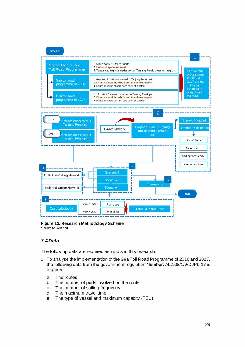
29
Figure 12. Research Methodology Scheme Source: Author
3.4 Data
The following data are required as inputs in this research:
1. To analyse the implementation of the Sea Toll Road Programme of 2016 and 2017, the following data from the government regulation Number: AL.108/1/9/DJPL-17 is required:
a. The routes b. The number of ports involved on the route c. The number of sailing frequency d. The maximum travel time e. The type of vessel and maximum capacity (TEU)
START
Master Plan of Sea Toll Road Programme
Sea toll road programme of 2016
Sea toll road programme of 2017
1. 5 hub ports, 19 feeder ports
2. Hub and spoke network
3. Tenau Kupang is a feeder port of Tanjung Perak to eastern regions
1. 6 routes, 3 routes connected to Tanjung Perak port
2. Direct network from hub port to sub-feeder port
3. Route and type of ship have been stipulated
1. 13 routes, 5 routes connected to Tanjung Perak port
2. Direct network from hub port to sub-feeder port
3. Route and type of ship have been stipulated
Sea tol road programmeof 2016 and 2017 are not in line with the master plan of sea toll road programme
1
Propose Tenau Kupang port as transhipment
port
3 routes connected to Tanjung Perak port
2016
5 routes connected to Tanjung Perak port
2017
Direct network
Supply loaded
Demand unloaded
No. of Ports
Type of ship
Sailing frequency
Container flow
2
Scenario I
Scenario II
Scenario III
3
Multi-Port-Calling Network
Hub-and-Spoke Network
4
Cost calculation
Time charter
Fuel costs
Port dues
Handling
5
Total Shipping Cost
Comparison
6
END

30
2. The demand and supply are reflected in the number of the containers loaded and unloaded at the ports is derived from the Tanjung Perak port report over the last five years.
3. To determine the components of total shipping costs, we obtain data from the Ministry of Transportation and Pelindo III corporation, the type of data is mentioned below:
a. Port facilities b. Port classification c. Port operation performance d. Port dues e. Terminal handling charge
4. Additional data required are obtained from:
a. The government Regulation(for the data on the distance between the ports in scenarios I and II);
b. Websites http://www.searoutes.com and http://ports.com (for the data on the distance between the ports in scenario III);
c. Indonesian Classification Agency (BKI register). The data necessary for the regression formula to determine the classification of the ship was collected from the list of specifications of container ships registered by this agency;
d. The Maersk Broker 2015 (for the data on the time charter); e. Shell Indonesia (which provided information on the fuel price); f. Central statistical bureau of Indonesia; g. Ministry of National Development Planning

31
Chapter 4 Overview on the Sea Toll Road Programme in Indonesia
In this chapter, we briefly describe the implementation of the Sea Toll Road Programme including the ports, routes and the type of ships used to distribute the containers from the port of Tanjung Perak to the South-Eastern parts of Indonesia. Next to that, we also provide information on the container flows to or from the port involved in this programme with regards to the ports connected to Tanjung Perak port-Surabaya. The number of containers or the number of loading and unloading of the containers in this chapter reflects on the number of supply and demand in the region.
4.2 Sea toll road programme 2016
In 2016, the Indonesian government adopted a strategy defining six routes connecting the main ports with sub-feeder ports located on the small islands of the country. These routes started in early 2016 and were operated by PELNI, a state-owned enterprise. The six predefined routes mentioned in the Decree of the General of Sea Transportation Number: Al.108/7/8/DJPL-2015 were the following:
Figure 13. Sea toll road programme of 2016 Source: Modified from Ministry of Transportation, 2016
In the implementation of the programme, the Indonesian government also provided subsidies to PELNI to operate its vessels in servicing the predefined routes. The subsidy was given for one year as per the Ministry of Transportation Regulation No. 85 of 2016. The total amount of subsidies given by the government of Indonesia is presented in Table 2.
Network 1 (N-1) : MV Mentari Freedom Network 2 (N-2) : MV Mentari Persada Network 3 (N-3) : MV Caraka Jaya Niaga III-22 Network 4 (N-4) : MV Meratus Ultima I Network 5 (N-5) : MV Caraka Jaya Niaga III-32 Network 6 (N-6) : MV Caraka Jaya Niaga III-4

32
Code Commission
days per voyage
Number of
voyage per year
Total (IDR) Equal to ($) The amount of
Subsidy per voyage ($)
N-1 28 10 40,668,163,920 3,068,209 306,821
N-2 28 9 51,874,769,187 3,913,692 434,855
N-3 28 10 24,064,232,082 1,815,526 181,553
N-4 28 9 54,605,831,070 4,119,737 457,749
N-5 28 9 27,115,638,795 2,045,739 227,304
N-6 21 14 20,661,364,946 1,558,797 111,343
Total Subsidy 218,990,000,000 16,521,699 1,719,624
Table 2. Total subsidy is given by the Government of Indonesia Source: Ministry of Transportation, 2016
Besides providing the subsidies, the Indonesian government also regulated tariffs for container distribution from or to the ports involved in this programme. This policy was only intended for container delivery by PELNI's vessels (Appendix 1). The number of sailing frequencies, types of ships, routes and the total of distances per each route are stipulated by the Indonesian government in the General Decree of Sea Transportation Number: Al.108/7/8/DJPL-2015.
Table 3. The routes of sea toll road programme 2016 Source: Modified from the decree of the General of Sea Transportation Number: Al.108/7/8/DJPL-2015
However, in this study, we only consider the routes starting from the port of Tanjung Perak, the main port and central distribution of cargo in the Western part of the country. Thus, we only take into account three routes, namely, N-1, N-2 and N-3. In order to serve the cargo distribution on each route, the Indonesian government defined the type of ships to be used in this programme. The name of the ships and its specifications can be explained in Appendix 2.
Code Total
(N.miles)
Tg Perak Wanci Namlea Fak-Fak Kaimana Timika
Kaimana Fak-Fak Namlea Wanci Tg Perak
Tg Perak Kalabahi Moa Saumlaki Dobo Merauke
Dobo Saumlaki Moa Kalabahi Tg Perak
Tg Perak Larantuka Lewoleba Rote Sabu Waingapu
Sabu Rote Lewoleba Larantuka Tg Perak
N-4 Tg Priok Makasar Manokwari Wasior Nabire Serui Biak
Serui Nabire Wasior Manokwari Makasar Tg Priok
N-5 Makasar Tahuna Lirung Morotai Tobelo Ternate Babang
Ternate Tobelo Morotai Lirung Tahuna Makasar
N-6 Tg Priok Tarempa Natuna Tarempa Tg Priok
Routes
N-1 3,426
N-2 3,874
N-3 2,078
4,644
2,612
1,400

33
4.2 Sea toll road programme 2017
In the beginning of 2017, the Indonesian government decided to change the routes after evaluating the implementation of Sea Toll Road Programme in 2016. Several routes were added so the total number of the routes increased to 13. Four of the routes were a change from the previous route. The government found on the routes established in 2016, the ships had to sail over very long distances for a very long time so that had to change.
Figure 14. Sea toll road programme of 2017 Source: Modified from Ministry of Transportation, 2017
In 2017, the Indonesian government also stipulated the type of the ships, the route involving the main ports and sub-feeder ports, the sailing frequency and the maximum time required by a ship to sail. Besides the number of routes, the main item that distinguishes the programme from the previous year is that the Indonesian government allowed the private shipping companies to participate by serving some certain routes which cannot be handled by PELNI because they do not have the facilities. The government opened bidding process to assess the private shipping company that has capability to serve the certain routes (Ministry of Transportation,
2017). Table 4 below, we present the routes established by the government regulation number: AL.108/1/9/DJPL-17 of 2017.

34
Table 4. The routes of sea toll road programme 2017 Source: The decree of the General of Sea Transportation Number: AL.108/1/9/DJPL-17 of 2017
As mentioned above, in this research, we only take into account the routes starting from the port of Tanjung Perak. In 2017, there are eight routes to be evaluated. However, we only consider five routes, which are N-1, N-2, N-3, N-11 and N-13. The main thinking behind this consideration is that N-4 and N-9 are still in the bidding process, while N-8 is assigned to serve general cargo.
In addition, the PELNI serves N-3, N-11 and N-13 by using three vessels as they are used to serve the routes on the 2016 Sea Toll Road Programme. The MV Freedom is used for serving N-13, the MV Mentari Perdana is used to serve N-11 and the MV Caraka Jaya Niaga III-22 is used to serve the same route (N-3). Meanwhile, Mentari Sejati Perkasa, a private shipping company, has won the tender to serve N-1 and N-2 routes. The detailed information related to the ships used can be seen in Appendix 2.
4.3 Profile of Tanjung Perak Port
The port of Tanjung Perak is the second busiest port in Indonesia after the port of Tanjung Priok. The Tanjung Perak port is located in Surabaya - the capital of East Java. The biggest port of Indonesia, the port of Tanjung Priok is located in Jakarta. Due to its geographical location, the Tanjung Perak port is a well-known gateway and distribution centre in the East of the country. According to the Ministry of Transportation (2011), Tanjung Perak port is classified as the main class port under the management of Pelindo III Corporation.
The port of Tanjung Perak consists of the branch of Tanjung Perak and three subsidiaries namely Berlian Jasa Terminal Indonesia (BJTI Port), Terminal Petikemas Surabaya (TPS) and Lamong Bay Terminal.
Code
Total Nautical
Miles
(N.miles)
N-1 Tg Perak Wanci Namlea Wanci Tg Perak 1,980
N-2 Tg Perak Kalabahi Moa Saumlaki Moa Kalabahi Tg Perak 2,374
N-3 Tg Perak Dompu Maumere Larantuka Lewoleba Rote Sabu Waingapu
Sabu Rote Lewoleba Larantuka Maumere Dompu Tg Perak
N-4 Tg Perak Bau-Bau Manokwari Bau-Bau Tg Perak 3,030
N-5 Makasar Tahuna Lirung Tahuna Makasar 1,760
N-6 Tg Priok Tarempa Natuna Tarempa Tg Priok 1,400
N-7 Tg Priok Enggano Mentawai Enggano Tg Priok 1,252
N-8 Tg Perak Belang2 Sangata Sebatik Tg Perak 1,880
N-9 Tg Perak Kisar Namrole Kisar Tg Perak 2,404
N-10 Makasar Tidore Tobelo Morotai Maba Gebe
Maba Morotai Tobelo Tidore Makasar
N-11 Tg Perak Saumlaki Dobo Merauke Dobo Saumlaki Tg Perak 3,864
N-12 Makasar Wasior Nabire Serui Biak
Serui Nabire Wasior Makasar
N-13 Tg Perak Fak-Fak Kaimana Timika Kaimana Fak-Fak Tg Perak 3,408
Routes
2,150
2,652
3,212

35
Figure 15. Lay out of Tanjung Perak port Source: modified from Teluk Lamong Bay website, 2017
The following is the detailed information regarding each terminal in the port of Tanjung Perak:
1. Tanjung Perak branch
Tanjung Perak branch has three terminals: Jamrud Terminal, Mirah Terminal and Nilam Terminal. Referring to the circular letter number: SE.8/PJ.04/TPR-2013 about the arrangement of the terminal at the port of Tanjung Perak branch-Surabaya, the management of Pelindo III Corporation has specified each terminal as dedicated area for:
No Name of Terminal Kade Meter Dedicated Area
1 Jamrud Terminal
a. North Jamrud 0 - 400 meter Passanger and Cruise Terminal
401 - 800 meter International General Cargo
801 - 1.200 meter International Dry Bulk
b. West Jamrud 0 - 210 meter International Dry Bulk
c. South Jamrud 0 - 210 meter Domestic Dry Bulk
211 - 800 meter Domestic General Cargo
d. Perak Kade 0 - 140 meter RoRo Terminal
2 Mirah Terminal 0 - 324 meter Domestic General Cargo
550 - 650 meter Off-shore and liquid bulk
651 - 860 meter RoRo Terminal
3 Nilam Terminal 60 - 330 meter Multipurpose Terminal
331 - 650 meter Domestic Container Terminal
650 - 930 meter Liquid Bulk Terminal
4 Kalimas Terminal Traditional Shipping
Table 5. Dedicated terminal at the port of Tanjung Perak branch-Surabaya Source: Pelindo III Corporation
Jamrud
Mirah
Berlian
Nilam
TPS
Lamong Bay

36
The Tanjung Perak branch has adequate facilities to serve the loading and unloading of cargoes and containers. The summary of the Tanjung Perak branch facilities is presented in the following Table 6.
1 Length 320 meter 6 Container Crane 4 units
2 Width 15 meter 7 RTG 5 units
3 Depth -8 m LWS 8 Reach Stacker -
4 Container Yard 34,880 m2 9 Head Truck 12 units
5 Capacity 20,100 TEU 10 Chassis 12 units
Table 6. Facility of domestic container terminal at Tanjung Perak branch-Surabaya Source: Pelindo III Corporation, 2017
2. Berlian Jasa Terminal Indonesia (BJTI Port)
The Berlian Jasa Terminal Indonesia is a subsidiary of the Pelindo III Corporation. The Berlian Terminal deals with domestic containers. The following Table is a summary of the facilities owned by the Berlian Terminal.
1 Length 1,620 meter 6 Harbour Mobile Crane 22 units
2 Width 15 meter 7 RTG 15 units
3 Depth -9.5 m LWS 8 Reach Stacker 4 units
4 Container Yard 45,790 m2 9 Head Truck + Chassis 25 units
5 Capacity 26,300 TEU 10 Forklift 12 units
Table 7. Facility of Berlian terminal Source: BJTI Port website, 2017
3. Terminal Petikemas Surabaya (TPS)
As well as the Berlian Jasa Terminal Indonesia, the Terminal Petikemas Surabaya is one of the subsidiaries of the Pelindo III Corporation, which is managed in cooperation with the DP World, the world-renowned terminal operator. The Terminal Petikemas Surabaya (TPS) handles the majority of international containers with the following facilities:
International Terminal Equipment
1 Length 1,000 meter 11 Container Crane 11 units
2 Width 50 meter 12 Head truck 80 units
3 Depth -13 m LWS 13 Chassis 124 units
4 Container Yard 35 ha 14 RTG 28 units
5 Capacity 32,223 TEU 15 Reach Stacker 6 units
Domestic Terminal 16 Reefer Plug 909 units
6 Length 450 meter 17 Sky Stacker 3 units
7 Width 50 meter 18 Dolly System 58 units
8 Depth -7.5 m LWS 19 Forklift Diesel 10 units
9 Container Yard 4.7 ha 20 Forklift Electric 8 units
10 Capacity 2,029 TEU 21 Trans lifter 7 units
Table 8. Facility of Terminal Petikemas Surabaya (TPS) Terminal Source: Terminal Petikemas Surabaya website, 2017

37
4. Terminal Lamong Bay
The Lamong Bay Terminal is the newest terminal that has just been built by the Terminal Teluk Lamong as a subsidiary of Pelindo III Corporation. The Lamong Bay Terminal started its operation in the beginning of 2015 and became the first green port in Indonesia (Lamong Bay Terminal, 2014). This Terminal is equipped with the modern equipment to support the increase in loading and unloading productivity as a solution to decrease the waiting time of the ships in the port of Tanjung Perak. Table 9 shows the complete range of facilities available in the terminal:
International Terminal Equipment
1 Length 500 meter 9 Straddle carrier 11 units
2 Width 50 meter 10 Automatic Stacking Crane 80 units
3 Depth -14 m LWS 11 Ship to Shore 124 units
4 Capacity of CY 4,860 TEU 12 CTT 28 units
Domestic Terminal 13 Reach Stacker 6 units
5 Length 450 meter 14 Grab ship unloader 909 units
6 Width 30 meter
7 Depth -7.5 m LWS
8 Capacity of CY 3,240 TEU
Table 9. Facility of Lamong Bay Terminal Source: Lamong Bay Terminal website, 2017
As the second busiest port in Indonesia, the port of Tanjung Perak has been able to handle the container flow over the last eight years. The detailed of its operation are specified in Figure 16 below:

38
Source: Annual report of Pelindo III Corporation, 2017 Figure 16. a) Container traffic per teminal b) International and Domestic container
4.4 Profile of Tenau Kupang Port
The port of Tenau Kupang is located in the East of Nusa Island. It is considered to be the main class port under the management of Pelindo III Corporation (Ministry of transportation Regulation, 2016). The Tenau Kupang port also manages three regional ports: Waingapu, Kalabahi and Ende/Ippi. Two of these ports, Waingapu and Kalabahi, are involved in the route of the Sea Toll Road Programme.
Figure 17. Layout of Tenau Kupang port Source: Google earth, 2017

39
The Tenau Kupang port consists of four terminals: the Multiguna terminal, the Nusantara terminal, the Local terminal and the multipurpose terminal. In addition, the local port authority has just developed new berthing facility in the area of the port of Tenau Kupang with the length of 125 meter, and it is currently under approval from the Ministry of Transportation to be operated by Pelindo III Corporation. It means that the port of Tenau Kupang has an additional capacity to serve the loading and unloading activities. The Table 10 below depicts the facilities of the port of Tenau Kupang.
1 Length 237.45 meter 6 Container Crane 2 units
2 Width 45.75 meter 7 RTG 3 units
3 Depth -12 m LWS 8 Reach Stacker 3 units
4 Container Yard 26,305 m2 9 Head Truck 8 units
5 Capacity 11,760 TEU 10 Chassis 8 units
Table 10. Facility of the port of Tenau Kupang Source: Head Office of Pelindo III Corporation, 2017
The port of Tenau Kupang is the main port in the Eastern region of Indonesia as its container flows continues to grow over the past eight years:
Figure 18. Container traffic at the port of Tenau Kupang Source: Annual report of the port of Tenau Kupang, 2017
4.5 The Demand and Supply
Because the sea toll road programme master plan will be implemented until 2019, we projected the demand and supply of containers (containing staple goods) based on the historical data of container flows from the 2012 to 2016 period as can be seen in Appendix 1. However, we realize that this demand projection is a limitation since we project the result for 2019 by using the average growth per year over the last five years of the container flows containing staple goods and a historical trend is no guarantee for the future. Moreover, we also face some data constraints. The issues are the following:

40
1. The data are obtained from the Port of Tanjung Perak. We manually selected and analysed the database of origin and destination of the containers especially with regard to the ports involved in this programme.
2. The database for the domestic container flows at Tanjung Perak port does not provide cargo information regarding what is in each container. This information is necessary as we only take into account containers containing staple goods as stipulated by Government regulation 71/2015. To address the problem, we processed the data of non-containers in order to know the percentage of staple goods loaded and unloaded at the port of Tanjung Perak. We found that 29 percent of the cargo were classified as staple goods. We then used this finding to multiply it with the total container flows to or from the ports involved in this program.
3. Based on the data, some of the ports (such as Lewoleba, Namlea, Rote, Saumlaki, Sabu and Moa) have only recently provided the container loading and unloading activities for 2016. This was after implementing the sea toll road program 2016. Therefore, we could not calculate the average growth rates per year to conduct demand projections. Thus, we have assumed 10 percent of growth per year to these ports refers to the port of Kaimana which has the lowest of the demand growth per year.
The Figure 19 below illustrates the demand projection based on the data in 2012-2016. Due to a significant difference between the destination ports, we divide the result into three different graphs as follows:

41
Figure 19. Projection of container flow by the port (TEU/year) Source: Author
We assume that the number of containers loaded at the destination port represents the demand, while the containers unloaded reflects the supply. The result of this container flow projection in every selected port in this study will be applied on the model analysis in order to calculate the total shipping costs. In addition, the routes for the three scenarios have been stipulated. What we then do is to put the number of containers based on each route. In general, we consider the number of containers per month instead of per year which means we divide the annual number of containers (TEU per year) by 12 to get data at a monthly basis.

42
--Blank Page--

43
Chapter 5 Data, Results and Analysis
In this Chapter, we present the results of our research and analyse them. First, we
analyse the fixed (Λ𝑡𝑚) and variable costs (𝜙𝑡
𝑚) per route in order to find out the total
shipping costs based on the mathematical model mentioned in chapter 3. The fixed cost is associated with the type of ship used and the route, while the variable cost is related to the number of containers carried by the ship. We also calculate the number of sailing frequencies for a certain period by dividing the total number of containers demanded at the destination port and TEU capacity of the ship used on each route. Further, the total cost will be obtained by multiplying the number of sailing frequencies a year and the total costs (i.e. the sum of fixed and variable costs). We apply this basic calculation to three different scenarios. Scenario I and II are similar since these scenarios deploy multi-port-calling networks in which a ship sails from the hub port to the destination ports as per the sea toll road programmes of 2016 and 2017. Meanwhile, Scenario III uses a hub-and-spoke network where we propose the Port of Tenau Kupang as a transhipment port to be the linking pin between the hub port and the sub-feeder ports. After conducting the calculations, we evaluate the results per scenario in order to determine which route generates the minimum total shipping costs for Indonesia.
5.1 Total Shipping Cost Data
Total shipping costs are the sum of fixed (Λ𝑡𝑚) and variable costs (𝜙𝑡
𝑚) multiplied by
the number of sailing frequencies for a certain period. In this section, we will describe the data and assumptions used in the total shipping cost calculations, such as charter rates, fuel costs, port dues, distance and handling charges.
5.1.1 Distance
The distance between port of origin and destination port is one of the key inputs to determine total shipping costs. These data are provided by the Indonesian government as stated in the regulations concerning the implementation of the sea toll road program in 2016 and 2017. In addition, we also use an online distance calculator (http://www.searoutes.com and http://ports.com) to measure the distances between the Port of Tenau Kupang and its destination ports in nautical miles. We require the distance to find out the total sea time vessels travel by dividing the distance between the ports by the speed of the ship (both in nautical miles). Next, this output will determine the amount of the fuel cost and charter cost at the sea. The Table of the distance in the Appendix 4 presents the distance matrix amongst the ports that have been used in each of the scenarios.
5.1.2 Ship Specification
The container ship size is regulated by the Indonesian government to serve the container distribution on each route within the sea toll road program. We consider applying this type of ship in our calculation. Since we only take into account the routes starting from the Port of Tanjung Perak, we found that there are five routes involving 15 sub-feeder ports that can be evaluated in this study where one ship is employed on each route. Table 11 below shows the name and the characteristics of each vessel used in this programme.

44
Name of Vessel DWT (Ton)
GT (Ton)
Capacity (20' Full) TEU
ME (HP)
AE (HP) Vt
(Knot)
Type of
ship
MV Mentari Freedom 5,314 4,303 192 4,168 1,331 11 t1
MV Mentari Perdana 4,985 4,180 199 3,940 1,313 11 t2
MV Caraka Jaya N III-22 3,650 3,258 135 3,013 1,176 11 t3
MV Nusantara Pelangi 3,106 2,997 115 2,635 1,137 11 t4
MV Mentari Perkasa 6,207 4,258 200 4,788 1,324 11 t5
Table 11. The type of the ship used in the sea toll road programme Source: Compiled by Author
Moreover, since in this study we propose a new route in Scenario III by involving the port of Tenau Kupang as a feeder port that serves as a transhipment hub connecting the main port (i.e. the port of Tanjung Perak) with the many sub-feeder ports, we need to determine the ship size used to carry the number of containers from Tanjung Perak port to the port of Tenau Kupang. To address with this problem, according to Maritime Technology course (Aalbers, 2016), we use a regression formula as can be seen in Appendix 5, where we can use the range of DWT to express the size of the ship including the gross tonnage (GT), TEU capacity, speed, engine power for Main Engine (ME) and Auxiliary Engine (AE) (. This calculation is based on the list of the ships and their specifications that already registered with the Indonesia Classification Bureau (BKI).
Type of Ship
Range of DWT DWT (Ton)
Payload GT ME AE Vt
(TEUs) (Ton) (HP) (HP) (knot)
ta < 2,000 2,000 80 1,800 1,900 1,000 11
tb 2,000 - 3,000 3,000 160 2,700 2,600 1,100 11
tc 3,000 - 5,000 5,000 320 4,500 4,000 1,400 12
td 5,000 - 7,500 7,500 520 6,800 5,700 1,800 14
te 7,500 - 10,000 10,000 720 9,000 7,400 2,200 15
tf 10,001 - 12,500 12,500 920 11,300 9,200 2,500 15
Table 12. Ship specification by ship size Source: Modified from Indonesia Classification Bureau (BKI)
We require the number of Gross Tonnage (GT) to calculate port dues including pilotage services, tugging services, anchoring fees and berth occupancy charges, while information on engine power is needed to figure out fuel consumption both at sea and in the port, allowing us to estimate fuel costs.
5.1.3 Ship Charter Rate
Basically, ship charter costs are used to replace operating costs, maintenance costs and capital costs. Ship charter rates obtained from Maersk Broker in 2015 provide the charter rates based on ship size. This charter rate covers capital, operating and periodic maintenance costs, excluding fuel costs, port dues and handling charges. Hence, in this study the total shipping costs are the sum of charter costs, fuel costs, port dues and container handling charges. The following Table 13 presents the time charter rate for a year based on the ship size from 200 until 5,199 TEU

45
Ship Size Charter Rate
(TEU) (USD/day)
200 - 399 1,900
400 - 649 4,969
650 - 899 5,594
900 - 1,299 7,800
1,300 - 1,999 9,609
2,000 - 2,999 9,834
3,000 - 3,949 11,608
3,950 - 5,199 14,364
Table 13. Time charter rate Source: Maersk Broker, 2015
5.1.4 Fuel Cost
In our calculations, we divide the fuel consumption into two parts: fuel consumption at sea (Ft) which is influenced by the type of the ship used and the route, and fuel consumption at the port (Fit), which depends on the type of ship and the time at the port. Based on these results, we can calculate the fuel cost both at sea and at port by multiplying the amount of fuel consumed with the fuel price.
The type of ship used determines the type of main engine and auxiliary engine to calculate the amount of fuel consumption. We assume that using SFOC (Specific Fuel Oil Consumption) for a Main Engine (ME) is 0.22 Litter/HP.hour. For an Auxiliary Engine (AE) this is 0.293 Litter/HP.hour. Furthermore, we can calculate the amount of fuel consumed by multiplying the operating time (hours), the level of engine power (HP) and SPOC (Litter/HP. Hour).
Additionally, we assume that the ships use High Speed Diesel (HSD) as their specific fuel. According to the Shell Indonesia website, the price of HSD in July 2017 is IDR 9,300 per litter or equal to USD 0.70 per litter (1 USD equals IDR 13,255).
5.1.5 Port Dues
Basically, ports dues applied in Indonesia consist of pilotage, towage, anchoring fee and berth occupancy charges. Piloting and tugging services are offered, depending on whether the port is a mandatory pilotage zone or not. This provision is stipulated by the Indonesian government. Piloting services are paid based on movement and Gross Tonnage (GT) per ship as well as the operating time required to perform the service. Likewise, this provision applies to tugging services. The anchoring fee is a cost incurred due to the use of the anchoring pool. Meanwhile, berth occupancy charges are paid because of the use of berth capacity. This cost depends on Gross Tonnage (GT) per ship per day and berthing time. Berthing time is calculated by dividing the number of containers loaded or unloaded and crane productivity.
Table 14 below shows the anchoring fee, berthing occupancy charge, piloting and towage costs for each of the 17 ports in our study.

46
No Name of Port Port Class Status
Mandato-
ry Pilotage
Zone
Anchoring fee (Per GT)
Berthing (Per
GT/day)
1 Dobo First Class Non Commercial No 0.007 0.006
2 Fak-Fak Fisrt Class Commercial No 0.007 0.006
3 Kaimana First Class Non Commercial No 0.007 0.006
4 Kalabahi First Class Commercial No 0.006 0.004
5 Larantuka First Class Non Commercial No 0.007 0.006
6 Lewoleba Second Class Non Commercial No 0.006 0.005
7 Merauke First Class Commercial Yes 0.007 0.007
8 Moa Fisrt Class Non Commercial No 0.007 0.006
9 Namlea First Class Non Commercial No 0.007 0.006
10 Rote Third Class Non Commercial No 0.006 0.005
11 Sabu Fisrt Class Non Commercial No 0.007 0.006
12 Saumlaki First Class Non Commercial No 0.007 0.006
13 Tg Perak Main Class Commercial Yes 0.100 0.131
14 Tenau Kupang Main Class Commercial Yes 0.006 0.004
15 Timika First Class Non Commercial No 0.007 0.006
16 Waingapu Second Class Commercial No 0.006 0.004
17 Wanci Second Class Non Commercial No 0.006 0.005
No Name of
Port
Mandatory Pilotage
Zone
Pilot Tug Boat
Fixed (per move)
Variable (per GT)
Fixed (per move)
Variable (per GT
per hour)
1 Dobo No - - - -
2 Fak-Fak No - - - -
3 Kaimana No - - - -
4 Kalabahi No - - - -
5 Larantuka No - - - -
6 Lewoleba No - - - -
7 Merauke Yes 4.936 0.003 24.142 0.000
8 Moa No - - - -
9 Namlea No - - - -
10 Rote No - - - -
11 Sabu No - - - -
12 Saumlaki No - - - -
13 Tanjung Perak
Yes 45.000 0.030 30.000 0.005
14 Tenau Kupang
Yes 8.299 0.004 38.839 0.000
15 Timika No - - - -
16 Waingapu No - - - -
17 Wanci No - - - -
Table 14. Port Dues Source: Compiled by Author

47
5.1.6 Container Handling Charge
This sub chapter highlights the issue of container handling charges (CHC) of each port based on information obtained from the respective port’s websites. In addition, we assume that handling fees for non-commercial ports is equal to handling fees for commercial ports, using shipping gear in the same region. Container handling charges are a combined package of stevedoring, lift on lift off (LOLO) and haulage. We also consider wharf charges for one unit (a container) in our calculations. Specifically, for handling large vessels in Scenario III, we also insert the loading and unloading equipment of container cranes into the equation and for both Tanjung Perak port and Tenau Kupang Port we take this into account.
No Name of Port Port Class Status
Terminal Handling Charge
20' full 20' empty
1 Dobo First Class Non Commercial 41.70 24.19
2 Fak-Fak Fisrt Class Commercial 41.70 24.19
3 Kaimana First Class Non Commercial 41.70 24.19
4 Kalabahi First Class Commercial 27.46 7.32
5 Larantuka First Class Non Commercial 27.16 5.21
6 Lewoleba Second Class Non Commercial 27.16 5.21
7 Merauke First Class Commercial 41.70 24.19
8 Moa Fisrt Class Non Commercial 32.90 19.54
9 Namlea First Class Non Commercial 32.90 19.54
10 Rote Third Class Non Commercial 18.11 10.86
11 Sabu Fisrt Class Non Commercial 18.11 10.86
12 Saumlaki First Class Non Commercial 41.70 24.19
13 Tanjung Perak Main Class Commercial 15.84 8.24
14 Tenau Kupang Main Class Commercial 22.63 13.58
15 Timika First Class Non Commercial 41.70 24.19
16 Waingapu Second Class Commercial 27.91 3.77
17 Wanci Second Class Non Commercial 32.90 19.54
Table 15. Container Handling Charge Source: Compiled by Author
5.1.7 Port operation
Port operation time can be described as the total time spent by the ship at port. Port operation times are the sum of berthing time and waiting time. To calculate berthing time, we require crane productivity, the number of cranes used and the number of containers loaded and unloaded at the port. While, waiting time is described as an idle time for a ship to reaching berth facilities. In general, the ship waits in an anchoring pool space provided by the port authority. The ship has to wait since the berthing facilities are, at that moment, being used by another ship or they have to wait for piloting or tugging service.
In addition, in Scenario I and II, we assume that the ships use the ship gear due to the size of the ship. While, in Scenario III, we use container cranes for loading or unloading activity. Moreover, we assume that the waiting time at the port of Tanjung Perak and the port of Tenau Kupang is four hours respectively, while other ports are assumed to have six hour waiting times, based on the port category.

48
Table 16 below informs us of the crane productivity (box per crane per hour) and idle time based on the port.
No Name of Port Port Class B/C/H Idle time (hour)
1 Dobo First Class 5 6
2 Fak-Fak Fisrt Class 12 6
3 Kaimana First Class 5 6
4 Kalabahi First Class 9 6
5 Larantuka First Class 5 6
6 Lewoleba Second Class 5 6
7 Merauke First Class 12 6
8 Moa Fisrt Class 5 6
9 Namlea First Class 5 6
10 Rote Third Class 5 6
11 Sabu Fisrt Class 5 6
12 Saumlaki First Class 5 6
13 Tanjung Perak Main Class 15 4
14 Tenau Kupang Main Class 14 4
15 Timika First Class 5 6
16 Waingapu Second Class 9 6
17 Wanci Second Class 5 6
Table 16. Crane Productivity and Idle Time Source: Compiled by Author
5.2 Results
This section describes the results of the model analysis used in this research paper. Calling to the previous explanation, we construct three scenarios where Scenario I and Scenario II use the multi-port-calling networks based on the implementation of the sea toll road program in 2016 and 2017, while Scenario III uses the hub-and-spoke network as described in the master plan of sea toll road program. The routes in Scenario I – sea toll road programme of 2016 and Scenario II – sea toll road programme of 2017 have been stipulated by the Indonesian government, so we follow these routes in order to calculate total shipping costs. Meanwhile, we build the routes in Scenario III by involving the port of Tenau Kupang as a transhipment port. As described before, the port of Tenau Kupang is set up as a feeder port and is connected with the main port (i.e. the Port of Tanjung Perak) according to the master plan of the sea toll road program (Ministry of development planning, 2015). Because the network in Indonesia recognises the main port, feeder ports and sub-feeder ports, Tenau Kupang port as a feeder port has the function of a transhipment port to connect the main port and the sub-feeder ports. We will compare the results of these three scenarios, and look at which one of the scenario generates the lowest total shipping costs.
In the implementation, all of the containers come from Tanjung Perak and will be distributed to the several destination ports involved on the routes in the different Scenarios. Likewise, containers from the destination ports will be carried back merely to the port of Tanjung Perak. This means that the vessel will visit all ports selected on the route. However, the container can merely be uploaded in the destination port.

49
Therefore, in order to simplify the calculation, we divide the costs into two different types of cost: fixed costs related to the type of ship used and the route, while variable costs related to the number of containers. The fixed costs cover all the ports visited by the ship (using connectivity between the ports), while the variable costs merely connect the port of Tanjung Perak and the destination port.
All scenarios constructed in this research paper use the same demand and supply data based on container flow projections in 2019. We divide the total demand and supply by 12 months as we would like to present the number of containers transported per voyage. If one ship is not allowed to carry all the containers demanded by the destination port on one route within a month due to constraints on the type of the ship used, we need more than one ship, whereby the total number of ships used should cover the total number of containers that needs to be transported. Next, we multiply the total number of ships used a month by 12 to find out the annual sailing frequencies.
A. Scenario I
We analyse three routes in the first scenario based on the implementation of the sea toll road programme 2016. In scenario I, we have three pendulum routes to be evaluated:
1. Tanjung Perak - Wanci - Namlea - Fak-Fak - Kaimana - Timika - Kaimana - Fak-Fak - Namlea - Wanci - Tanjung Perak
2. Tanjung Perak - Kalabahi - Moa - Saumlaki - Dobo - Merauke - Dobo - Saumlaki - Moa - Kalabahi - Tanjung Perak
3. Tanjung Perak - Larantuka - Loweloba - Rote - Sabu - Waingapu - Sabu - Rote - Lewoleba - Larantuka - Tanjung Perak
In order to get a more detailed explanation of our calculation, we will explain step by step by using network 1. These steps will also be applied on the other routes in this scenario as can be seen in Appendix 4. First, we have to capture the distance among the ports on this route as well as the type of the ship where we follow the Indonesian government. Network 1 is serviced by the type of ship with a capacity of 192 TEU. The distance travelled can be explained by the information presented in Table 17
O/D TPK WNC NML FAK KMN TMK
TPK - 700 990 1,316 1,498 1,713
WNC 700 - 290 616 798 1,013
NML 990 290 - 326 508 723
FAK 1,316 616 326 - 182 397
KMN 1,498 798 508 182 - 215
TMK 1,713 1,013 723 397 215 -
Table 17. Distance (in Nautical Mile) Source: The decree of the General of Sea Transportation Number: Al.108/7/8/DJPL-2015
As explained before, we divided the cost into two different type of cost: fixed cost (USD) and unit cost (USD/TEU/Nmile) based on variable cost. Starting with the fixed cost, the following Table 18 presents the connectivity. First, we manually input 1 or 0 into the Table of connectivity (Xij). 1 (one) indicates that there is connectivity between a port and the next port. If there is no connectivity, we input 0. The connectivity is followed the routes as stipulated by the government of Indonesia.
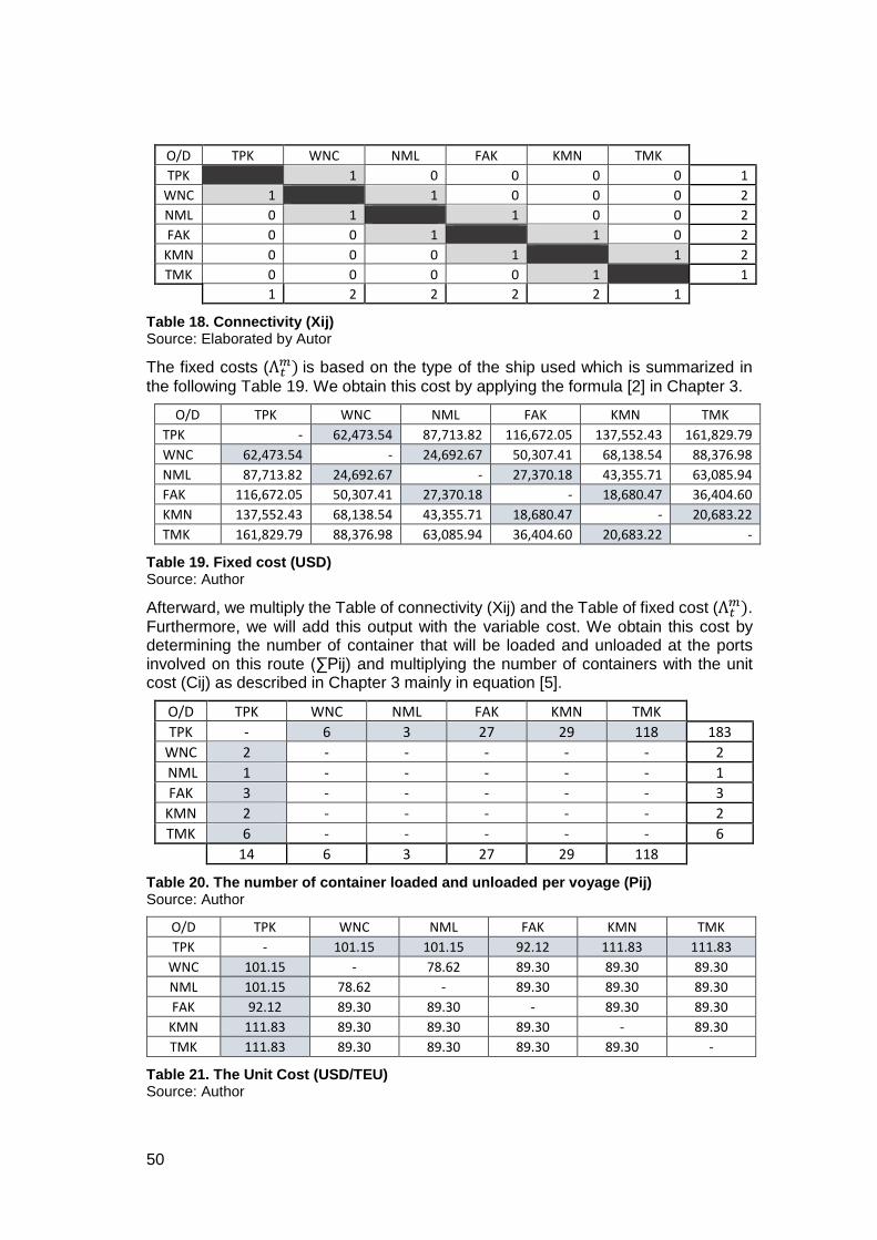
50
O/D TPK WNC NML FAK KMN TMK
TPK 1 0 0 0 0 1
WNC 1 1 0 0 0 2
NML 0 1 1 0 0 2
FAK 0 0 1 1 0 2
KMN 0 0 0 1 1 2
TMK 0 0 0 0 1 1
1 2 2 2 2 1
Table 18. Connectivity (Xij) Source: Elaborated by Autor
The fixed costs (Λ𝑡𝑚) is based on the type of the ship used which is summarized in
the following Table 19. We obtain this cost by applying the formula [2] in Chapter 3.
O/D TPK WNC NML FAK KMN TMK
TPK - 62,473.54 87,713.82 116,672.05 137,552.43 161,829.79
WNC 62,473.54 - 24,692.67 50,307.41 68,138.54 88,376.98
NML 87,713.82 24,692.67 - 27,370.18 43,355.71 63,085.94
FAK 116,672.05 50,307.41 27,370.18 - 18,680.47 36,404.60
KMN 137,552.43 68,138.54 43,355.71 18,680.47 - 20,683.22
TMK 161,829.79 88,376.98 63,085.94 36,404.60 20,683.22 -
Table 19. Fixed cost (USD) Source: Author
Afterward, we multiply the Table of connectivity (Xij) and the Table of fixed cost (Λ𝑡𝑚).
Furthermore, we will add this output with the variable cost. We obtain this cost by determining the number of container that will be loaded and unloaded at the ports involved on this route (∑Pij) and multiplying the number of containers with the unit cost (Cij) as described in Chapter 3 mainly in equation [5].
O/D TPK WNC NML FAK KMN TMK
TPK - 6 3 27 29 118 183
WNC 2 - - - - - 2
NML 1 - - - - - 1
FAK 3 - - - - - 3
KMN 2 - - - - - 2
TMK 6 - - - - - 6 14 6 3 27 29 118
Table 20. The number of container loaded and unloaded per voyage (Pij) Source: Author
O/D TPK WNC NML FAK KMN TMK
TPK - 101.15 101.15 92.12 111.83 111.83
WNC 101.15 - 78.62 89.30 89.30 89.30
NML 101.15 78.62 - 89.30 89.30 89.30
FAK 92.12 89.30 89.30 - 89.30 89.30
KMN 111.83 89.30 89.30 89.30 - 89.30
TMK 111.83 89.30 89.30 89.30 89.30 -
Table 21. The Unit Cost (USD/TEU) Source: Author

51
Further, total shipping cost derived by adding the fixed cost and variable cost. Moreover, we also calculate the time travel required for a ship to sail from the port of Tanjung Perak to the ports of destination and returns to the origin port. The total travel time is sum of the time at the sea (days) and the port that have been explained in the previous section. The result will be gained by multiply the following Table 22 and the Table of connectivity as can be seen in Table 23.
O/D TPK WNC NML FAK KMN TMK
TPK - 4 5 6 7 8
WNC 4 - 2 4 4 5
NML 5 2 - 3 3 4
FAK 6 4 3 - 2 3
KMN 7 4 3 2 - 2
TMK 8 5 4 3 2 -
Table 22. Time travel (days) Source: Author
Moreover, we also determine the number of vessels are needed per month in order to generate the number of sailing frequencies per year. The result is one of the factors in determining the total shipping cost per route. As explained before, we divide the total demand and supply by 12 months as we would like to present the number of containers transported per voyage. If one ship is not allowed to carry all the containers demanded by the destination port on one route within a month due to constraints on the type of the ship used, we need more than one ship, whereby the total number of ships used should cover the total number of containers that needs to be transported. For example, the total containers demanded on the route N-1 is 722 TEU per month, where the total capacity of a ship used on this route is 192 TEU. Further, we divide the total containers demanded on one route by the total capacity of a ship used. We obtain that this route requires four ships. Moreover, we also consider the total travel time of one ship sailing from the origin port to the destination ports and back. As long as the total travel time less than one month, means that this route does not need additional vessel. The number of ships needed on one route per month can be explained by the information presented in Table 23.
In addition, we also calculate the utilization of vessel as one of the key factor in determining the effectiveness and efficiency of a vessel use. We calculate the utilization rate by dividing the total containers carried per voyage and the total capacity of a ship used. Table 23 informs us the utilization of vessel used to transport the container per route.
After calculating all of these networks in scenario I by applying those steps above, we generate the result as follows
The Route Ship's
Capacity (Teu)
Number of ships needed
per month
Number of Sailing
Frequency per year
Traveling time
(days)
Utilizati-on of
vessel
Total Shipping Cost per route
N-1 192 4 48 26 95% $ 15,797,353
N-2 199 4 48 26 98% $ 16,995,622
N-3 135 2 24 14 79% $ 2,167,448
Total Shipping Cost $ 34,960,423
Table 23. The result of Scenario I Source: Author

52
B. Scenario II
Scenario II is constructed, based on the implementation of the sea toll road program 2017. The number of ports involved in this scenario is the same compared to Scenario I. However, the total networks in this scenario increases to five networks as Networks 1 and 2, that were used in Scenario I, are divided into two different networks, while the Network 3 remains the same as it was in Scenario I. The Indonesian government decided to change the routes since Networks 1 and 2 involved to many ports in one network. Scenario II therefore consists of the following five networks:
1. Tanjung Perak - Wanci - Namlea - Wanci - Tanjung Perak
2. Tanjung Perak - Fak-Fak - Kaimana - Timika - Kaimana - Fak-Fak - Tanjung Perak
3. Tanjung Perak - Kalabahi - Moa - Saumlaki - Moa - Kalabahi - Tanjung Perak
4. Tanjung Perak - Dobo - Merauke - Dobo -Tanjung Perak
5. Tanjung Perak - Larantuka - Loweloba - Rote - Sabu - Waingapu - Sabu - Rote - Lewoleba - Larantuka - Tanjung Perak
Our calculations follow the same methodological steps as under Scenario I. Table 24 shows the results of the total shipping cost in each network in Scenario II
The Route Ship's
Capacity (Teu)
Number of ships needed
per month
Number of Sailing
Frequency per year
Traveling time
(days)
Utilizati-on of
vessel
Total Shipping Cost per route
N-1 115 1 12 12 28% $ 1,347,655
N-13 192 4 48 20 91% $ 15,112,078
N-2 200 1 12 16 57% $ 2,963,685
N-11 199 4 48 20 84% $ 16,486,649
N-3 135 2 24 14 79% $ 2,167,448
Total Shipping cost $ 38,077,514
Table 24. The result of Scenario II Source: Author
According to the result above, the level of vessel utilization on the route N-1 and N-2 are very low. Moreover, this ineffectiveness potentially leads to an increase in total shipping costs as we found that the total shipping cost in scenario II which reflects to the implementation of the sea toll road programme of 2017 has increased compared to the implementation in 2016. As mentioned before, the implementation of sea toll road programme in 2017 is a remedial step executed by the Indonesian government in improving the implementation of the previous programme.
C. Scenario III
We develop Scenario III on the basis of a hub-and-spoke network. As explained before, the Port of Tenau Kupang is part of this scenario. Since this port, as a feeder port to connect the port of Tanjung Perak to sub-feeder ports, it has a main function as a transhipment port. The calculations made are slightly different from those in Scenarios I and II, because in this Scenario we have to determine the type of ships used to carry containers from the port of Tanjung Perak to Tenau Kupang Port. Referring to Table 12, we select a ship with a capacity of 920 TEU. The main reason behind this selection is that this type of vessel is able to carry the number of containers demanded by the sub-feeder ports each month. We assume that this type of vessel is available.

53
Moreover, we have to multiply the container handling charges of loading and unloading at the port of Tenau Kupang by two. We assume that the stacking time for the container to be loaded and unloaded at the port of Tenau Kupang is five days. This means that there will be an additional ten days on a round time.
We construct 15 networks in this Scenario based on the number of sub-feeder ports selected in this study. The container will be carried from the port of Tanjung Perak and transhipped via the port of Tenau Kupang before being delivered to the sub-feeder ports. The use of a bigger vessel to transport the number of containers from Tanjung Perak to Tenau Kupang leads to the achievement of economies of scale. Our calculations show that the fixed costs and variable costs incurred on the route from Tanjung Perak to Tenau Kupang are $ 122,012.41 per voyage and $ 81.525 per TEU, respectively. These costs include the double container handling charge, stacking cost, double port dues and also the fuel cost. The calculation can be explained by the information presented in Appendix 3. These results will serve as inputs into the network calculations for this Scenario in a similar was we did in Scenarios I and II.
The Table 25 below depicts the result of the total shipping cost per network in scenario III
The Route Name of the Port
Ship's Capacity
(Teu)
Number of ships needed
per month
Number of Sailing
Frequency per year
Traveling time
(days)
Utilizati-on of
vessel
Total Shipping Cost per route
H&S 1 Wanci 115 1 12 16 18% $ 1,052,916
H&S 2 Namlea 115 1 12 16 10% $ 1,068,166
H&S 3 Fak-Fak 115 1 12 18 92% $ 1,709,060
H&S 4 Kaimana 135 1 12 18 84% $ 1,705,864
H&S 5 Timika 200 3 36 20 79% $ 8,475,156
H&S 6 Saumlaki 115 1 12 16 10% $ 1,075,838
H&S 7 Kalabahi 135 1 12 14 68% $ 856,503
H&S 8 Moa 115 1 12 16 10% $ 1,074,570
H&S 9 Dobo 115 1 12 16 88% $ 1,306,072
H&S 10 Merauke 200 3 36 20 96% $ 9,878,574
H&S 11 Larantuka 115 1 12 12 30% $ 615,557
H&S 12 Lewoleba 115 1 12 12 17% $ 558,138
H&S 13 Rote 115 1 12 12 2% $ 511,451
H&S 14 Sabu 115 1 12 12 10% $ 538,235
H&S 15 Waingapu 192 1 12 16 76% $ 1,144,394
Total Shipping cost $ 31,570,494
Table 25. The result of Scenario III Source: Author
Based on the Table above, the calculation of Scenario III generates the lowest total shipping cost. However, since there are some ports with a low number of containers, we consider to create a hub-and-spoke network with indirect shipments. The main thinking behind this consideration is that we have to optimise the use of the vessel. We combine these ports in one route while the other ports which have enough demand remains the same using the direct hub-and-spoke, as follows:
1. Tanjung Perak – Tenau Kupang – Larantuka – Lewoleba – Wanci – Namlea – Wanci – Lewoleba – Larantuka – Tenau Kupang – Tanjung Perak (defined as H&S indirect 1)

54
2. Tanjung Perak – Tenau Kupang – Kalabahi – Moa – Saumlaki – Moa – Kalabahi – Tenau Kupang – Tanjung Perak (defined as H&S indirect 2)
3. Tanjung Perak – Tenau Kupang – Rote – Sabu – Waingapu – Sabu – Rote – Tenau Kupang – Tanjung Perak (defined as H&S indirect )
After changing the network by combining these ports that have low levels of container demand and that are close to each other, we generate the results presented in Table 26.
The Route Name of the Port
Ship's Capacity
(Teu)
Number of ships needed
per month
Number of Sailing
Frequency per year
Traveling time
(days)
Utilizati-on of
vessel
Total Shipping Cost per route
H&S Indirect 1 115 1 12 22 85% $ 1,606,853
H&S Indirect 2 192 1 12 26 73% $ 1,941,555
H&S Indirect 3 192 1 12 18 84% $ 1,174,409
H&S 3 Fak-Fak 115 1 12 18 92% $ 1,709,060
H&S 4 Kaimana 135 1 12 18 84% $ 1,705,864
H&S 5 Timika 200 3 36 20 79% $ 8,475,156
H&S 9 Dobo 115 1 12 16 88% $ 1,306,072
H&S 10 Merauke 200 3 36 20 96% $ 9,878,574
Total Shipping cost $ 27,797,543
Table 26. The result of combining direct and indirect H&S network in Scenario III Source: Author
We obtain that combining direct and direct hub-and-spoke network is more efficient to be applied in Scenario III.
5.3 Cost Comparison Analysis
After conducting an analysis based on three scenarios as described in the previous sections, this section turns to the results are comparing them with each other. In order to provide a good explanation and comparison between each scenario, all of the results are summarised in Table 27 and can be seen in Appendix 6.
No Scenario
Average of Total Travel Time (days)
Average of the vessel
utilization
Total Shipping cost
1 Scenario I 22 91% $ 34,960,423
2 Scenario II 16 68% $ 38,077,514
3 Scenario III
a) Direct 16 46% $ 31,570,494
b) Combining direct and indirect 20 85% $ 27,797,543
Table 27. The comparison of each scenario Source: Author

55
According to the Table 27 above, scenario II leads to the highest total shipping cost compared to scenario I and III. It is caused by the low vessel utilization. The ships have to sail per month and carry a low number of the containers. However, the number of sailing frequency in scenario II is less than scenario I, it makes sense since the number of the ports that should be visited by a ship on one route is less than scenario I.
Furthermore, Table 27 also indicates that applying hub-and-spoke network on delivering the container from the port of Tanjung Perak to the South-East of Indonesia can reduce the total shipping cost. We also combine the direct and indirect shipment on the basis hub-and-spoke network and the result is more efficient compared to the other results. Even though, the total round time increases compared to the direct hub-and-spoke network, results show that roundtrip travel time is shorter than scenario I.
This result therefore answers the main question of this study: the proposed network in which we involve the port of Tenau Kupang clearly contributes to reducing the total shipping costs of distributing a container from the western region of Indonesia (represented by the Port of Tanjung Perak) to the South-Eastern region of Indonesia.

56
--Blank Page--

57
Chapter 6 Conclusion and Recommendation
6.1 Conclusion
Nowadays, the government of Indonesia is attempting to implement the design of a sea toll road program as an integrated system that uses the hub-and-feeder concept to reduce logistics costs and to lower the price disparity between the western and eastern regions of Indonesia. During 2015-2019, the Indonesian government focuses on developing 24 strategic ports involved in this program. However, several issues especially with regard to the higher logistic cost and price disparity need to be solved as soon as possible. Therefore, in 2016, the Indonesian government stipulated the six routes under the sea toll road program for 2016. These routes applied multi-port-calling networks, where a ship takes one month to sail from the port of Tanjung Perak to the port of selected in this programme.
In 2017, the Indonesian government changed the routes after evaluating the implementation of the sea toll road program in 2016. The number of the routes was increased to 13, where four of these routes resulted from a split-up of previous routes. As in 2016, the implementation of the sea toll road program in 2017 used a multi-port-calling network. Referring to the design of the sea toll road program that will be implemented by 2019, the network to be used in these programs is the hub-and-spoke network. A container will be transported from the main port to the feeder port before being further distributed to the sub-feeder ports. However, in the implementation of the sea toll road program in 2016 and 2017, the function of the feeder ports has been ignored since the container was directly distributed from the main port to the sub-feeder ports.
As explained above, we conduct this study in order to obtain an in- depth analysis of how and what best networks can be applied by the Indonesian government to distribute a container from the western regions to the South-Eastern parts of Indonesia. We take into account the routes starting from the port of Tanjung Perak (as the gateway and distribution centre) from the west to the east of Indonesia. We construct three scenarios. Scenario I consist of three networks based on the implementation of the sea toll road program in 2016. Scenario II consists of five networks based on the routes stipulated by the sea toll road program 2017. Finally, Scenario III also involves the Port of Tenau Kupang as a transhipment port. The main consideration behind this final Scenario is that the Port of Tenau Kupang is set up as a feeder port and is connected to the port of Tanjung Perak according to the master plan of the sea toll road program (BAPPENAS, 2015). Because the network in Indonesia recognizes the different nodes: main port, feeder port and sub-feeder port, Tenau Kupang port as a feeder port has a transhipment function to connect the main port and the sub-feeder ports.
After conducting the analysis, we obtain four results based on three scenarios where two of these results are generated by Scenario III. We construct 15 networks in Scenario III based on the number of the ports selected in this study. Since the network used in Scenario III is hub-and-spoke, there are some ports that face low demand and generate low ship utilization rates. Hence, we consider to combine these ports with the low demand in order to optimize the use of the ship.
Overall, scenario II generates the highest total shipping cost compared to scenarios I and III. The Indonesian government has already changed the routes and made the network operate over shorter distances. However, the low vessel utilization leads to

58
higher costs for container distribution in Scenario II. In contrast, scenario I produces a high level of sailing frequencies compared to other scenarios. The reason for this is that the ship has a maximum capacity and should carry the container to several ports. While, combining direct and indirect hub-and-spoke network in Scenario III shows the best result of this study. The hub-and-spoke model allows the use of the bigger sized vessels for container demand from the port of Tanjung Perak to the port of Tenau Kupang to achieve economies of scale. So, the proposed model by involving the port of Tenau Kupang, contributes to reduce total shipping costs of container distribution from the western regions of Indonesia that are represented by the port of Tanjung Perak to South-Eastern part of Indonesia.
6.2 Recommendation
The result of this research can assist the Indonesian government in order to create an effective and efficient route in terms of distributing container from the West to East of Indonesia under the sea toll road programme.
Due to the limitation of this research, we suggest for the further research to consider other the main ports are located in Western regions of Indonesia as the port of origin, such as: the port of Belawan and Tanjung Priok. Moreover, other feeder ports as defined in the master plan of the sea toll road programme also can be taken into account.
Furthermore, we merely focus on the total shipping cost incurred for distributing containers from the port of origin to the destination port without considering the total logistics costs from the shipper to the buyer. As a suggestion, it will be better, if the future research also calculate receiving and delivery cost. It can provide more depth analysis and close to the real condition.
59
Bibliography
Aalbers, A (2016). Development of ships. Presentation. Erasmus University Rotterdam, Rotterdam, The Netherlands
BAPPENAS, 2015. Laporan Implementasi Konsep Tol Laut 2015-2019, Jakarta: Kementerian Perencanaan dan Pembangunan Nasional.
BJTI Port, 2017. The port facilities. [Online] Available at: http://www.bjtiport.co.id/index.php?option=com_content&view=article&id=236&Itemid=142 [Accessed 1 August 2017].
Business Dictionary, 2017. Business Dictionary. [Online] Available at: http://www.businessdictionary.com/definition/essential-good.html [Accessed 21 July 2017].
Central Statistical Bureau of Indonesia, 2017. BPS. [Online] Available at: https://www.bps.go.id/website/brs_ind/brsInd-20170208123344.pdf [Accessed 1 May 2017].
Chen, C. & Zeng, Q., 2010. Designing container shipping network under changing demand and freight rates. Transport, 25(1), pp. 46-57.
Christiansen, M., Fagerholt, K. & Ronen, D., 2004. Ship routing and schedulling: Status and perspective. Transportation Science, 38(1), pp. 1-18.
Hsu, C.-I. & Hsieh, Y.-P., 2007. Routing, ship size, and sailing frequency decision-making for a hub-and-spoke container network. Mathematical and Computer Modelling, 45(7-8), pp. 899-916.
Imai, A., Nishimura, E., Papadimitriou, S. & Liu, M., 2006. The economic viability of container mega-ships. Transportation Reasearch Part E: Logistics and Transportation Review, 42(1), pp. 21-41.
Imai, A., Shintani, K. & Papadimitriou, S., 2009. Multi-port vs Hub-and-Spoke port calls by containership. Transportation Research Part E: Logistics and Transportation Review, 45(5), pp. 740-757.
Lamong Bay Terminal, 2017. Overview of Lamong Bay Terminal. [Online] Availabe at: http://www.teluklamong.co.id/ [Accessed 1 August 2017]
Lazuardi, S. D., 2015. Analyzing the National Logistics System through Integrated and Efficient Logistics Network : Study of Container Shipping Connectivity in Indonesia. MSc Thesis. Rotterdam, The Netherland: Erasmus University Rotterdam.
Lun, Y. V. & Browne, M., 2009. Fleet mix in container shipping operations. International Journal of Shipping and Transport Logistics, 1(2), pp. 103-118.
Maersk Broker, 2015. Container Market. [Online] Available at: www.soefart.dk/app/doc/Container Market.pdf [Accessed 1 May 2017]

60
Meng, Q. & Wang, S., 2011. Liner shipping service network design with empty container repositioning. Transportation Research Part E: Logistics and Transportation Review, 47(5), pp. 695-708.
Ministry of Transportation, 2015. Network of the sea freight transport of 2016 Number: Al.108/7/8/DJPL-2015.
Ministry of Transportation, 2017. Network of the sea freight transport of 2017 Number: Al.108/1/9/DJPL-2017.
Mourao, M., Pato, M. & Paixao, A., 2002. Ship assignment with hub and spoke constraints. Maritime Policy & Management, 29(2), pp. 135-150.
Mulder, J. & Dekker, R., 2014. Methods for strategic liner shipping network design. European Journal of Operational Research, 235(2), pp. 367-377.
Notteboom, T. E., 2004. Container shipping and ports: An overview. Review of Network Economics, 3(2), pp. 86-106.
Notteboom, T. & Rodrigue, J.-P., 2008. Containerisation, Box logistics and Global Supply Chains: The Integration of Ports and Liner Shipping Networks. 23(Palgrave Macmillan), pp. 152-174.
Pelindo III Corporation, 2016. Annual report 2016. [Online] Available at https://www.pelindo.co.id/en/info-investor/laporan/q/annual-report [Accessed 13 May 2017].
Pelindo III Corporation, 2017. Company Profile. [Online] Available at: https://www.pelindo.co.id/profil-perusahaan/cabang-anak-perusahaan/cabang-perusahaan/q/tanjung-perak [Accessed 1 August 2017].
Polat, O., Gunther, Hans-Otto & Kulak, O., 2014. The feeder network design problem: Application to container services in the Black sea region. Maritime Economics and Logistics, 16(3), pp. 343-369 (27).
Port.com, 2017. Sea route and distance. [Online] Available at: http://ports.com/sea-route/ [Accessed 6 May 2017].
Pryun, J.F.J., (2016) Ship finance. Presentation. Erasmus University Rotterdam, Rotterdam, The Netherlands.
Ronen, D., 1983. Cargo ships routing and scheduling: Survey of models and problem. European Journal of Operational Research, 12(2), pp. 119-126.
Ronen, D., 1993. Ship scheduling: The last decade. European Journal of Operational Research, 71(3), pp. 325-333.
Searoutes.com, 2017. Distance calculator, weather routing and voyage planning. [Online] Available at: https://www.searoutes.com/routing?speed=13&panama=true&suez=true&kiel=true [Accessed 6 May 2017].
61
Simlitabnas, 2011. Pendahuluan Masterplan Percepatan dan Perluasan Pembangunan Ekonomi Indonesia(MP3EI)2011-2025. [Online] Available at: http://simlitabmas.dikti.go.id/html/tab3611.htm [Accessed 5 May 2017].
Shell Indonesia, 2017. Fuel price. [Online] Available at : http://www.shell.co.id/ [Accessed 2 May 2017].
Stopford, M., 2009. Maritime Economics. In: Third Edition. London & New York: Routledge Taylor and Francis Group, pp. 219-221.
Terminal Petikemas Surabaya, 2017. the port facilities. [Online] Available at http://www.tps.co.id/id-id/fasilitas/dermaga [Accessed 1 August 2017].
The cabinet secretariat of the RI, 2014. Sekertariat Kabinet Republik Indonesia. [Online] Available at: http://setkab.go.id/category/mp3ei/ [Accessed 5 May 2017].
The Indonesian government, 2015. Stipulation and storage of staple and essential goods Number. 71 of 2015.
The World Bank, 2016. Global Ranking 2016. [Online] Available at: https://lpi.worldbank.org/international/global [Accessed 21 July 2017].
Van Rijn, L., 2015. Service network design for liner shipping in Indonesia. Bachelor Thesis. Rotterdam, The Netherlands : Erasmus University Rotterdam.
Wardana, W., 2014. Centre Gravity Model and Network Design to Determine Route of Liner Shipping. MSC Thesis. Rotterdam, The Netherlands : Erasmus University Rotterdam.

62
--Blank Page--

63
Appendices
Appendix 1. The demand and Supply
This table merely presents the number of containers loaded and unloaded at the Port of Tanjung Perak especially with regard to the ports involved in this programme.
Table 28. Total number of containers in TEU (Full)
Table 29. Total number of containers contain of staple goods in TEU (Full)
Supply Demand Supply Demand Supply Demand Supply Demand Supply Demand
DOBO - - - - - - - - 756 2,788
FAK-FAK 203 869 224 908 220 951 120 1,029 254 2,046
KAIMANA 60 2,370 106 2,541 157 2,942 214 3,506 134 3,492
KALABAHI - - - - - - - 1,520 326 2,835
LARANTUKA - - 194 465 145 627 140 638 207 856
LEWOLEBA - - - - - - - - 207 638
MERAUKE 1,236 7,284 1,358 10,442 1,622 10,351 2,055 10,414 2,770 14,022
NAMLEA - - - - - - - - 102 344
ROTE - - - - - - - - 12 66
SAUMLAKI - - - - - - - - 44 344
TIMIKA 824 5,645 694 4,451 1,054 7,481 1,022 6,210 865 10,268
WAINGAPU - - 302 1,546 270 2,184 508 2,378 544 3,300
WANCI - - - - - - - - 207 638
SABU - - - - - - - - 44 344
MOA - - - - - - - - 44 344
20162015Name of the
port
2012 2013 2014
Supply Demand Supply Demand Supply Demand Supply Demand Supply Demand
DOBO - - - - - - - - 219 807
FAK-FAK 59 252 65 263 64 275 35 298 74 592
KAIMANA 17 686 31 736 45 852 62 1,015 39 1,011
KALABAHI - - - - - - - 440 94 821
LARANTUKA - - 56 135 42 182 41 185 60 248
LEWOLEBA - - - - - - - - 60 185
MERAUKE 358 2,109 393 3,024 470 2,997 595 3,015 802 4,060
NAMLEA - - - - - - - - 30 100
ROTE - - - - - - - - 3 19
SAUMLAKI - - - - - - - - 13 100
TIMIKA 239 1,635 201 1,289 305 2,166 296 1,798 250 2,973
WAINGAPU - - 87 448 78 632 147 689 158 956
WANCI - - - - - - - - 60 185
SABU - - - - - - - - 13 100
MOA - - - - - - - - 13 100
2015 20162012 2013 2014Name of the
port

64
Appendix 2. The Ships used
1. MV Freedom
No Remark Information No Remark Information
1 Name of vessel MV Freedom 7 TEU Capacity 192 20' full
2 Name of Operator PELNI 8 GT 4,303
3 Name of the Owner Mentari Sejati
Perkasa 9 LOA 108
4 Type Container vessel 10 DWT 5,314
5 Year of Built 1993 11 Number of Ship Gear 2
6 Speed 11 12 Owned or Charter Charter
Source: Mentari Line website, 2017
2. MV Mentari Perdana
Source: Modified from Mentariline
No Remark Information No Remark Information
1 Name of vessel MV Mentari Perdana 7 TEU Capacity 199 20' full
2 Name of Operator PELNI 8 GT 4,180
3 Name of the Owner Mentari Sejati Perkasa 9 LOA 115
4 Type Container Vessel 10 DWT 4,985
5 Year of Built 1997 11 Number of Ship Gear 2
6 Speed 11 12 Owned or Charter Charter

65
Source: Mentari Line website, 2017
3. MV Caraka Jaya Niaga III-22
No Remark Information No Remark Information
1 Name of vessel MV Caraka Jaya Niaga III-22 7 TEU Capacity 115 20' full
2 Name of Operator PELNI 8 GT 3,258
3 Name of the Owner Mentari Sejati Perkasa 9 LOA 98
4 Type Semi-Container Vessel 10 DWT 3,650
5 Year of Built 1993 11 Number of Ship Gear
2
6 Speed 11 12 Owned or Charter Charter
Source: www.marinetraffic.com
Source: Maritime observer website, 2017

66
4. MV Nusantara Pelangi
No Remark Information No Remark Information
1 Name of vessel MV Nusantara Pelangi 7 TEU Capacity 115 20' full
2 Name of Operator Mentari Sejati Perkasa 8 GT 2,997
3 Name of the Owner - 9 LOA 97
4 Type Container Vessel 10 DWT 3,106
5 Year of Built 2008 11 Number of Ship Gear 2
6 Speed 11 12 Owned or Charter Charter
Source: Maritime Traffic website, 2017
Source: Tirto website, 2017
5. MV Mentari Perkasa
No Remark Information No Remark Information
1 Name of vessel MV Mentari Prakarsa 7 TEU Capacity 115 20' full
2 Name of Operator Mentari Sejati Perkasa 8 GT 4,258
3 Name of the Owner - 9 LOA 112
4 Type Container Vessel 10 DWT 6,207
5 Year of Built 2008 11 Number of Ship Gear 2
6 Speed 11.8 12 Owned or Charter Charter
Source: Modified from Mentariline
Source: Maritime Traffic website, 2017

67
Appendix 3. Fixed Cost and Unit Cost per each route
ROUTE No of Teu Capacity Distance (Di) Speed Sea Time Port time Ft Fixed Cost
nm v (days) days USD US$ US$/Teu
TPK-WNC 100 192 700 11 3 0.71 1,212 2,873 41,085 17,304 10,115.36 62,473.54 101.15
TPK-NML 100 192 990 11 4 0.71 1,212 2,873 57,775 25,853 10,115.36 87,713.82 101.15
TPK-FAK 100 192 1,307 11 5 0.71 1,212 2,873 76,392 36,195 9,211.59 116,672.05 92.12
TPK-KMN 100 192 1,498 11 6 0.71 1,212 2,873 87,305 46,162 11,183.25 137,552.43 111.83
TPK-TMK 100 192 1,713 11 7 0.71 1,212 2,873 100,144 57,601 11,183.25 161,829.79 111.83
WNC-TPK 100 192 700 11 3 1.83 63 7,436 41,085 17,304 8,516.04 65,887.49 85.16
WNC-NML 100 192 290 11 1 0.79 40 3,211 16,691 4,751 7,862.03 24,692.67 78.62
WNC-FAK 100 192 616 11 2 0.79 40 3,211 35,949 11,108 8,929.92 50,307.41 89.30
WNC-KMN 100 192 798 11 3 0.79 40 3,211 46,862 18,026 8,929.92 68,138.54 89.30
WNC-TMK 100 192 1,013 11 4 0.79 40 3,211 59,059 26,067 8,929.92 88,376.98 89.30
NML-TPK 100 192 990 11 4 1.83 69 7,436 57,775 25,853 8,516.04 91,133.89 85.16
NML-WNC 100 192 290 11 1 0.79 42 3,211 16,691 4,751 7,862.03 24,695.40 78.62
NML-FAK 100 192 326 11 1 0.79 42 3,211 19,258 4,858 8,929.92 27,370.18 89.30
NML-KMN 100 192 508 11 2 0.79 42 3,211 29,530 10,573 8,929.92 43,355.71 89.30
NML-TMK 100 192 723 11 3 0.79 42 3,211 42,369 17,464 8,929.92 63,085.94 89.30
FAK-TPK 100 192 1,316 11 5 0.92 49 3,718 77,034 36,329 6,544.37 117,129.56 65.44
FAK-WNC 100 192 616 11 2 0.79 46 3,211 35,949 11,108 7,862.03 50,313.47 78.62
FAK-NML 100 192 326 11 1 0.79 46 3,211 19,258 4,858 7,862.03 27,373.51 78.62
FAK-KMN 100 192 182 11 1 0.79 46 3,211 10,913 4,511 8,929.92 18,680.47 89.30
FAK-TMK 100 192 397 11 2 0.79 46 3,211 23,110 10,038 8,929.92 36,404.60 89.30
KMN-TPK 100 192 1,498 11 6 1.83 69 7,436 87,305 46,162 8,516.04 140,972.50 85.16
KMN-WNC 100 192 798 11 3 0.79 42 3,211 46,862 18,026 7,862.03 68,141.28 78.62
KMN-NML 100 192 508 11 2 0.79 42 3,211 29,530 10,573 7,862.03 43,355.71 78.62
KMN-FAK 100 192 182 11 1 0.79 42 3,211 10,913 4,511 8,929.92 18,677.14 89.30
KMN-TMK 100 192 215 11 1 0.79 42 3,211 12,839 4,591 8,929.92 20,683.22 89.30
TMK-TPK 100 192 1,713 11 7 1.83 69 7,436 100,144 57,601 8,516.04 165,249.85 85.16
TMK-WNC 100 192 1,013 11 4 0.79 42 3,211 59,059 26,067 7,862.03 88,379.71 78.62
TMK-NML 100 192 723 11 3 0.79 42 3,211 42,369 17,464 7,862.03 63,085.94 78.62
TMK-FAK 100 192 397 11 2 0.79 42 3,211 23,110 10,038 8,929.92 36,401.28 89.30
TMK-KMN 100 192 215 11 1 0.79 42 3,211 12,839 4,591 8,929.92 20,683.22 89.30
TPK-KLB 100 199 731 11 3 0.71 1,185 2,957 40,051 17,528 8,136.97 61,720.34 81.37
TPK-MOA 100 199 963 11 4 0.71 1,185 2,957 53,401 25,596 10,246.47 83,138.48 102.46
TPK-SML 100 199 1,187 11 5 0.71 1,185 2,957 65,538 34,524 11,126.51 104,202.62 111.27
Unit costFixed
portion (αit)
Daily charter at
port i (OtWi)

68
ROUTE No of Teu Capacity Distance (Di) Speed Sea Time Port time Ft Fixed Cost
nm v (days) days USD US$ US$/Teu
TPK-DBO 100 199 1,427 11 5 0.71 1,185 2,957 78,888 37,305 11,314.37 120,334.23 113.14
TPK-MRK 100 199 1,937 11 7 0.71 1,185 2,957 106,802 60,369 9,009.96 171,312.16 90.10
KLB-TPK 100 199 731 11 3 1.17 40 4,870 40,051 17,528 7,101.23 62,488.73 71.01
KLB-MOA 100 199 232 11 1 0.79 33 3,304 12,743 4,705 7,927.58 20,785.93 79.28
KLB-SML 100 199 456 11 2 0.79 33 3,304 24,880 10,421 8,807.62 38,638.93 88.08
KLB-DBO 100 199 696 11 3 0.79 33 3,304 38,230 17,301 8,995.48 58,868.69 89.95
KLB-MRK 100 199 1,206 11 5 0.79 33 3,304 66,751 34,777 8,720.10 104,865.53 87.20
MOA-TPK 100 199 963 11 4 1.92 69 8,000 53,401 25,596 8,647.15 87,067.04 86.47
MOA-KLB 100 199 232 11 1 0.79 41 3,304 12,743 4,705 7,364.01 20,793.96 73.64
MOA-SML 100 199 224 11 1 0.79 41 3,304 12,137 4,680 8,807.62 20,161.85 88.08
MOA-DBO 100 199 464 11 2 0.79 41 3,304 25,487 10,472 8,995.48 39,304.36 89.95
MOA-MRK 100 199 974 11 4 0.79 41 3,304 54,008 25,697 8,720.10 83,050.88 87.20
SML-TPK 100 199 1,187 11 5 1.92 69 8,000 65,538 34,524 8,647.15 108,131.19 86.47
SML-KLB 100 199 456 11 2 0.79 41 3,304 24,880 10,421 7,364.01 38,646.96 73.64
SML-MOA 100 199 224 11 1 0.79 41 3,304 12,137 4,680 7,927.58 20,161.85 79.28
SML-DBO 100 199 240 11 1 0.79 41 3,304 13,350 4,730 8,995.48 21,426.08 89.95
SML-MRK 100 199 750 11 3 0.79 41 3,304 41,265 17,680 8,720.10 62,290.14 87.20
DBO-TPK 100 199 1,427 11 5 1.92 69 8,000 78,888 37,305 8,647.15 124,262.79 86.47
DBO-KLB 100 199 696 11 3 0.79 41 3,304 38,230 17,301 7,364.01 58,876.71 73.64
DBO-MOA 100 199 464 11 2 0.79 41 3,304 25,487 10,472 7,927.58 39,304.36 79.28
DBO-SML 100 199 240 11 1 0.79 41 3,304 13,350 4,730 8,807.62 21,426.08 88.08
DBO-MRK 100 199 510 11 2 0.79 41 3,304 27,914 10,674 8,720.10 41,933.96 87.20
MRK-TPK 100 199 1,937 11 7 0.96 196 4,000 106,802 60,369 6,618.12 171,366.94 66.18
MRK-KLB 100 199 1,206 11 5 0.79 191 3,304 66,751 34,777 7,364.01 105,023.52 73.64
MRK-MOA 100 199 974 11 4 0.79 191 3,304 54,008 25,697 7,927.58 83,200.83 79.28
MRK-SML 100 199 750 11 3 0.79 191 3,304 41,265 17,680 8,807.62 62,440.10 88.08
MRK-DBO 100 199 510 11 2 0.79 191 3,304 27,914 10,674 8,995.48 42,083.92 89.95
TPK-LRK 100 135 656 11 3 0.54 905 1,635 27,843 12,537 8,467.46 42,921.17 84.67
TPK-LWB 100 135 808 11 3 0.54 905 1,635 33,876 13,292 8,467.46 49,708.00 84.67
TPK-RTE 100 135 840 11 3 0.54 905 1,635 35,268 13,466 7,464.05 51,274.19 74.64
TPK-SBU 100 135 920 11 4 0.54 905 1,635 38,981 18,573 7,464.05 60,093.90 74.64
TPK-WGP 100 135 1,039 11 4 0.54 905 1,635 43,621 19,346 7,326.68 65,507.90 73.27
LRK-TPK 100 135 656 11 3 1.38 44 4,151 27,843 12,537 7,363.82 44,575.47 73.64
LRK-LWB 100 135 32 11 0 0.63 29 1,887 1,392 - 6,790.24 3,307.80 67.90
LRK-RTE 100 135 184 11 1 0.63 29 1,887 7,889 3,348 5,786.82 13,152.31 57.87
LRK-SBU 100 135 264 11 1 0.63 29 1,887 11,137 3,483 5,786.82 16,536.05 57.87
LRK-WGP 100 135 383 11 1 0.63 29 1,887 16,242 3,696 6,767.61 21,853.37 67.68
LWB-TPK 100 135 808 11 3 1.38 40 4,151 33,876 13,292 7,363.82 51,358.80 73.64
Unit costFixed
portion (αit)
Daily charter at
port i (OtWi)

69
ROUTE No of Teu Capacity Distance (Di) Speed Sea Time Port time Ft Fixed Cost
nm v (days) days USD US$ US$/Teu
LWB-LRK 100 135 32 11 0 0.63 27 1,887 1,392 - 6,790.24 3,306.14 67.90
LWB-RTE 100 135 32 11 0 0.63 27 1,887 1,392 - 5,786.82 3,306.14 57.87
LWB-SBU 100 135 112 11 0 0.63 27 1,887 4,641 - 5,786.82 6,554.54 57.87
LWB-WGP 100 135 231 11 1 0.63 27 1,887 9,745 3,425 6,767.61 15,084.22 67.68
RTE-TPK 100 135 840 11 3 1.38 37 4,151 35,268 13,466 7,363.82 52,921.48 73.64
RTE-LRK 100 135 184 11 1 0.63 25 1,887 7,889 3,348 6,790.24 13,148.99 67.90
RTE-LWB 100 135 32 11 0 0.63 25 1,887 1,392 - 6,790.24 3,304.49 67.90
RTE-SBU 100 135 80 11 0 0.63 25 1,887 3,248 - 5,786.82 5,160.71 57.87
RTE-WGP 100 135 199 11 1 0.63 25 1,887 8,353 3,367 6,767.61 13,632.38 67.68
SBU-TPK 100 135 920 11 4 1.38 44 4,151 38,981 18,573 7,363.82 61,748.20 73.64
SBU-LRK 100 135 264 11 1 0.63 29 1,887 11,137 3,483 6,790.24 16,536.05 67.90
SBU-LWB 100 135 112 11 0 0.63 29 1,887 4,641 - 6,790.24 6,556.20 67.90
SBU-RTE 100 135 80 11 0 0.63 29 1,887 3,248 - 5,786.82 5,164.03 57.87
SBU-WGP 100 135 119 11 0 0.63 29 1,887 5,105 - 6,767.61 7,020.26 67.68
WGP-TPK 100 135 1,029 11 4 0.88 27 2,642 43,621 19,346 6,245.67 65,636.14 62.46
WGP-LRK 100 135 383 11 1 0.63 23 1,887 16,242 3,696 6,790.24 21,848.06 67.90
WGP-LWB 100 135 231 11 1 0.63 23 1,887 9,745 3,425 6,790.24 15,080.56 67.90
WGP-RTE 100 135 199 11 1 0.63 23 1,887 8,353 3,367 5,786.82 13,630.38 57.87
WGP-SBU 100 135 119 11 0 0.63 23 1,887 5,105 - 5,786.82 7,014.94 57.87
TKP-WNC 100 115 463 11 2 0.50 247 1,312 17,045 6,666 9,128.08 25,270.32 91.28
TKP-NML 100 115 510 11 2 0.50 247 1,312 18,669 6,802 9,128.08 27,028.95 91.28
WNC-TKP 100 115 463 11 2 1.21 34 3,169 17,045 6,666 8,081.66 26,915.25 80.82
NML-TKP 100 115 510 11 2 1.21 37 3,169 18,669 6,802 8,081.66 28,676.72 80.82
TKP-FAK 100 115 863 11 3 0.50 247 1,312 31,655 11,826 8,920.90 45,039.98 89.21
TKP-KMN 100 135 681 11 3 0.58 252 1,761 28,772 12,653 10,643.83 43,437.58 106.44
TKP-TMK 100 200 909 11 3 0.75 267 3,143 61,207 20,224 11,969.31 84,841.72 119.69
FAK-TKP 100 115 863 11 3 0.67 29 1,749 31,655 11,826 6,806.59 45,259.30 68.07
KMN-TKP 100 135 681 11 3 1.38 44 4,151 28,772 12,653 8,529.52 45,619.59 85.30
TMK-TKP 100 200 909 11 3 1.92 71 8,033 61,207 20,224 9,854.99 89,534.91 98.55
TKP-KLB 100 135 138 11 1 0.58 252 1,761 6,033 3,270 7,894.22 11,315.72 78.94
TKP-MOA 100 115 516 11 2 0.50 247 1,312 19,074 6,836 9,128.08 27,468.61 91.28
TKP-SML 100 115 516 11 2 0.50 247 1,312 19,074 6,836 10,008.12 27,468.61 100.08
KLB-TKP 100 135 138 11 1 0.88 27 2,642 6,033 3,270 7,411.37 11,971.67 74.11
MOA-TKP 100 115 516 11 2 1.21 37 3,169 19,074 6,836 8,081.66 29,116.38 80.82
SML-TKP 100 115 516 11 2 1.21 37 3,169 19,074 6,836 8,081.66 29,116.38 80.82
TKP-DBO 100 115 516 11 2 0.50 247 1,312 19,074 6,836 10,195.97 27,468.61 101.96
Unit costFixed
portion (αit)
Daily charter at
port i (OtWi)

70
Detail Calculation of the total shipping cost from the port of Tanjung Perak to Tenau Kupang port
ROUTE No of Teu Capacity Distance (Di) Speed Sea Time Port time Ft Fixed Cost
nm v (days) days USD US$ US$/Teu
TKP-MRK 100 200 1,023 11 4 0.75 267 3,143 68,582 28,194 9,656.64 100,186.49 96.57
DBO-TKP 100 115 822 11 3 1.21 37 3,169 30,438 11,674 8,081.66 45,318.04 80.82
MRK-TKP 100 200 1,023 11 4 0.96 197 4,016 68,582 28,194 7,817.70 100,989.52 78.18
TKP-LRK 100 115 121 11 0 0.50 247 1,312 4,464 - 8,632.41 6,022.91 86.32
TKP-LWB 100 115 89 11 0 0.50 247 1,312 3,247 - 8,632.41 4,805.40 86.32
TKP-RTE 100 115 89 11 0 0.50 247 1,312 3,247 - 7,628.99 4,805.40 76.29
TKP-SBU 100 115 104 11 0 0.50 247 1,312 3,653 - 7,628.99 5,211.24 76.29
TKP-WGP 100 192 279 11 1 0.75 268 3,042 16,049 4,725 8,728.21 24,083.08 87.28
LRK-TKP 100 115 121 11 0 1.21 37 3,169 4,464 - 8,081.66 7,670.68 80.82
LWB-TKP 100 115 89 11 0 1.21 34 3,169 3,247 - 8,081.66 6,450.32 80.82
RTE-TKP 100 115 89 11 0 1.21 31 3,169 3,247 - 8,081.66 6,447.48 80.82
SBU-TKP 100 115 104 11 0 1.21 37 3,169 3,653 - 8,081.66 6,859.01 80.82
WGP-TKP 100 192 279 11 1 1.13 40 4,563 16,049 4,725 8,200.09 25,376.61 82.00
Unit costFixed
portion (αit)
Daily charter at
port i (OtWi)
ROUTE No of Teu Distance (Di) Speed Sea Time Ft
nm v (days) PO PD USD
TPK-TKP 800 795 15 2 3.63 3.71 10 2,670 358 93,833 75,099 28,627
Fixed
portion
(αit) PO
Total time
(d)
Fixed
portion
(αit) PD
Daily charter
at port i
(OtWi)
Port time (days)
ROUTE PO (βi) PD (βj)
Total
handling
fee (USD) Total Ot/Ri
USD USD USD Fixed US$ US$/Teu
TPK-TKP 20.05 25.58 45.62 35.90 65,219.70 122,012.41 81.525
Variable
Cost

71
Appendix 4. The Total Shipping Cost Calculation
1. Scenario I a. Network 1
Connectivity (Network 1)
Xij
O/D TPK WNC NML FAK KMN TMK
TPK 1 0 0 0 0 1
WNC 1 1 0 0 0 2
NML 0 1 1 0 0 2
FAK 0 0 1 1 0 2
KMN 0 0 0 1 1 2
TMK 0 0 0 0 1 1
1 2 2 2 2 1
Cargo Allocation
Pij
O/D TPK WNC NML FAK KMN TMK
TPK - 6 3 27 29 118 183
WNC 2 - - - - - 2
NML 1 - - - - - 1
FAK 3 - - - - - 3
KMN 2 - - - - - 2
TMK 6 - - - - - 6
14 6 3 27 29 118
Ship capacity constraint
∑(t∈T) Ut = 192 TEU 95%
O/D TPK WNC NML FAK KMN TMK
TPK - 6 3 27 29 118 183
WNC 2 - - - - - 2
NML 1 - - - - - 1
FAK 3 - - - - - 3
KMN 2 - - - - - 2
TMK 6 - - - - - 6
14 6 3 27 29 118
O/D TPK WNC NML FAK KMN TMK
TPK - 700 990 1,316 1,498 1,713
WNC 700 - 290 616 798 1,013
NML 990 290 - 326 508 723
FAK 1,316 616 326 - 182 397
KMN 1,498 798 508 182 - 215
TMK 1,713 1,013 723 397 215 -
Distance (Nm)

72
b. Network 2
Fixed Cost (USD)
O/D TPK WNC NML FAK KMN TMK
TPK - 62,473.54 87,713.82 116,672.05 137,552.43 161,829.79
WNC 62,473.54 - 24,692.67 50,307.41 68,138.54 88,376.98
NML 87,713.82 24,692.67 - 27,370.18 43,355.71 63,085.94
FAK 116,672.05 50,307.41 27,370.18 - 18,680.47 36,404.60
KMN 137,552.43 68,138.54 43,355.71 18,680.47 - 20,683.22
Variable Cost (USD/TEU/Nml)
O/D TPK WNC NML FAK KMN TMK
TPK - 101.15 101.15 92.12 111.83 111.83
WNC 101.15 - 78.62 89.30 89.30 89.30
NML 101.15 78.62 - 89.30 89.30 89.30
FAK 92.12 89.30 89.30 - 89.30 89.30
KMN 111.83 89.30 89.30 89.30 - 89.30
TMK 111.83 89.30 89.30 89.30 89.30 -
Time (days)
O/D TPK WNC NML FAK KMN TMK
TPK - 4 5 6 7 8
WNC 4 - 2 4 4 5
NML 5 2 - 3 3 4
FAK 6 4 3 - 2 3
KMN 7 4 3 2 - 2
TMK 8 5 4 3 2 -
Objective Function
Total Cost per voyage $ 329,112
Number of sail ing frequency 48 calls/year
Total Cost per year $ 15,797,353
Total travel time per voyage 26 days
Connectivity (Network 2)
Xij
O/D TPK KLB MOA SML DBO MRK
TPK 0 1 0 0 0 0 1
KLB 1 0 1 0 0 0 2
MOA 0 1 1 0 0 2
SML 0 0 1 0 1 0 2
DBO 0 0 0 1 0 1 2
MRK 0 0 0 0 1 0 1
1 2 2 2 2 1

73
Pij
O/D TPK KLB MOA SML DBO MRK
TPK - 23 3 3 23 144 196
KLB 3 - - - - - 3
MOA 1 - - - - - 1
SML 1 - - - - - 1
DBO 6 - - - - - 6
MRK 31 - - - - - 31
42 23 3 3 23 144
Ship capacity constraint
∑(t∈T) Ut = 199 TEU 98%
O/D TPK KLB MOA SML DBO MRK
TPK - 23 3 3 23 144 196
KLB 3 - - - - - 3
MOA 1 - - - - - 1
SML 1 - - - - - 1
DBO 6 - - - - - 6
MRK 31 - - - - - 31
42 23 3 3 23 144
O/D TPK KLB MOA SML DBO MRK
TPK - 731 963 1,187 1,427 1,937
KLB 731 - 232 456 696 1,206
MOA 963 232 - 224 464 974
SML 1,187 456 224 - 240 750
DBO 1,427 696 464 240 - 510
MRK 1,937 1,206 974 750 510 -
Distance (Nm)
Fixed Cost (USD)
O/D TPK KLB MOA SML DBO MRK
TPK - 61,720.34 83,138.48 104,202.62 120,334.23 171,312.16
KLB 61,720.34 - 20,785.93 38,638.93 58,868.69 104,865.53
MOA 83,138.48 20,785.93 - 20,161.85 39,304.36 83,050.88
SML 104,202.62 38,638.93 20,161.85 - 21,426.08 62,290.14
DBO 120,334.23 58,868.69 39,304.36 21,426.08 - 41,933.96
MRK 171,312.16 104,865.53 83,050.88 62,290.14 41,933.96 -
Variable Cost (USD/TEU/Nml)
O/D TPK KLB MOA SML DBO MRK
TPK - 81.37 102.46 111.27 113.14 90.10
KLB 81.37 - 79.28 88.08 89.95 87.20
MOA 102.46 79.28 - 88.08 89.95 87.20
SML 111.27 88.08 88.08 - 89.95 87.20
DBO 113.14 89.95 89.95 89.95 - 87.20
MRK 90.10 87.20 87.20 87.20 87.20 -

74
c. Network 3
Time
O/D TPK KLB MOA SML DBO MRK
TPK - 4 5 6 7 9
KLB 4 - 2 3 4 6
MOA 5 2 - 2 3 5
SML 6 3 2 - 2 4
DBO 7 4 3 2 - 3
MRK 9 6 5 4 3 -
Objective Function
Total Cost per voyage $ 354,075
Number of sail ing frequency 48 calls/year
Total Cost per year $ 16,995,622
Total travel time per voyage 26 days
Connectivity (Network 3)
Xij
O/D TPK LRK LWB RTE SBU WGP
TPK 0 0 0 0 0 0 0
LRK 1 0 1 0 0 0 2
LWB 0 1 0 1 0 0 2
RTE 0 0 1 0 1 0 2
SBU 0 0 0 1 0 1 2
WGP 0 0 0 0 1 0 1
1 1 2 2 2 1
Cargo Allocation
Pij
O/D TPK LRK LWB RTE SBU WGP
TPK - 17 10 1 6 73 107
LRK 3 - - - - - 3
LWB 3 - - - - - 3
RTE 1 - - - - - 1
SBU 1 - - - - - 1
WGP 12 - - - - - 12
20 17 10 1 6 73
Ship capacity constraint
∑(t∈T) Ut = 135 TEU 79%
O/D TPK LRK LWB RTE SBU WGP
TPK - 17 10 1 6 73 107
LRK 3 - - - - - 3
LWB 3 - - - - - 3
RTE 1 - - - - - 1
SBU 1 - - - - - 1
WGP 12 - - - - - 12
20 17 10 1 6 73
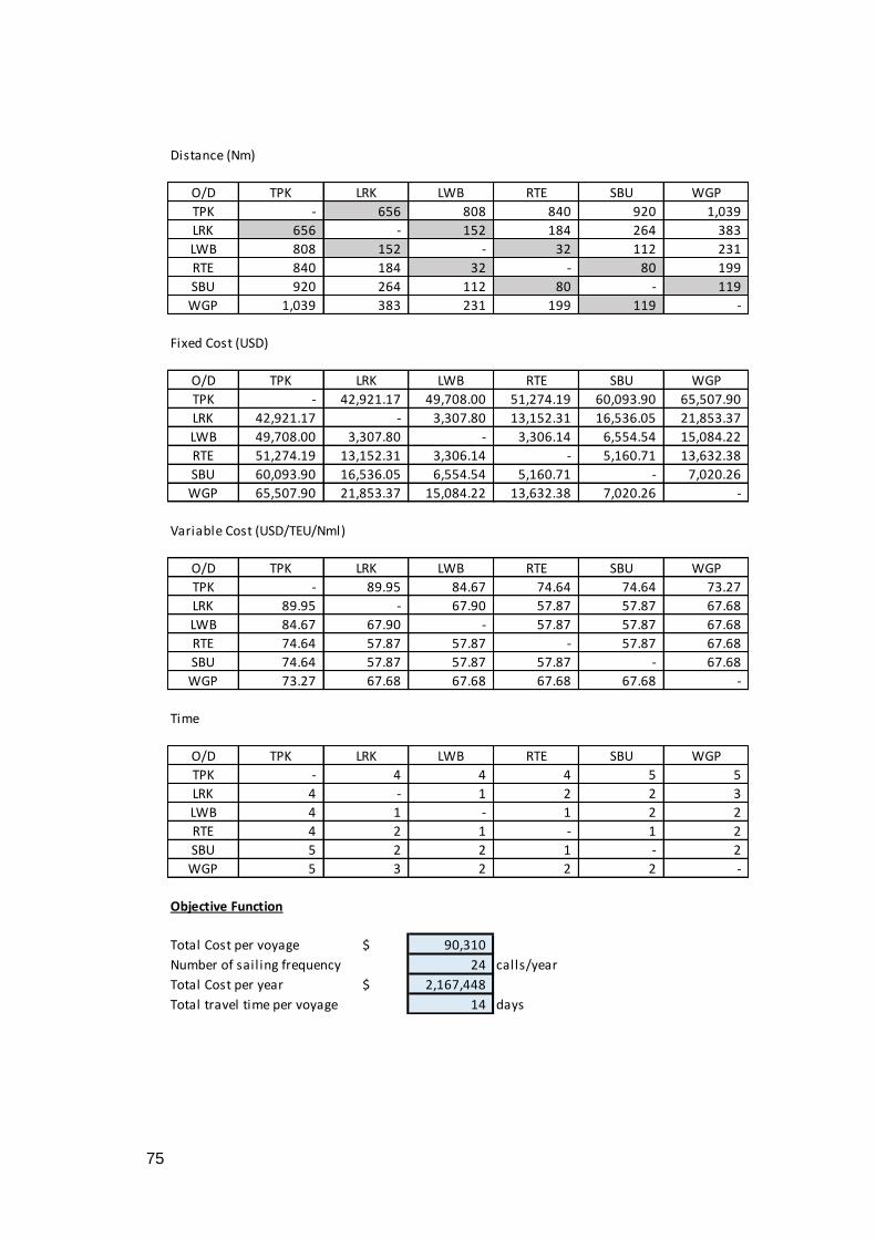
75
O/D TPK LRK LWB RTE SBU WGP
TPK - 656 808 840 920 1,039
LRK 656 - 152 184 264 383
LWB 808 152 - 32 112 231
RTE 840 184 32 - 80 199
SBU 920 264 112 80 - 119
WGP 1,039 383 231 199 119 -
Fixed Cost (USD)
O/D TPK LRK LWB RTE SBU WGP
TPK - 42,921.17 49,708.00 51,274.19 60,093.90 65,507.90
LRK 42,921.17 - 3,307.80 13,152.31 16,536.05 21,853.37
LWB 49,708.00 3,307.80 - 3,306.14 6,554.54 15,084.22
RTE 51,274.19 13,152.31 3,306.14 - 5,160.71 13,632.38
SBU 60,093.90 16,536.05 6,554.54 5,160.71 - 7,020.26
WGP 65,507.90 21,853.37 15,084.22 13,632.38 7,020.26 -
Variable Cost (USD/TEU/Nml)
O/D TPK LRK LWB RTE SBU WGP
TPK - 89.95 84.67 74.64 74.64 73.27
LRK 89.95 - 67.90 57.87 57.87 67.68
LWB 84.67 67.90 - 57.87 57.87 67.68
RTE 74.64 57.87 57.87 - 57.87 67.68
SBU 74.64 57.87 57.87 57.87 - 67.68
WGP 73.27 67.68 67.68 67.68 67.68 -
Time
O/D TPK LRK LWB RTE SBU WGP
TPK - 4 4 4 5 5
LRK 4 - 1 2 2 3
LWB 4 1 - 1 2 2
RTE 4 2 1 - 1 2
SBU 5 2 2 1 - 2
WGP 5 3 2 2 2 -
Objective Function
Total Cost per voyage $ 90,310
Number of sail ing frequency 24 calls/year
Total Cost per year $ 2,167,448
Total travel time per voyage 14 days
Distance (Nm)

76
2. Scenario II (N-3 remains the same as in Scenenario I) a. Network 1
Connectivity (Network 1)
Xij
O/D TPK WNC NML
TPK - 1 - 1
WNC 1 - 1 2
NML - 1 - 1
1 2 1
Cargo Allocation
Pij
O/D TPK WNC NML
TPK - 21 11 32
WNC 6 - - 6
NML 3 - - 3
9 21 11
Ship capacity constraint
∑(t∈T) Ut = 115
O/D TPK WNC NML
TPK - 21 11 32
WNC 6 - - 6
NML 3 - - 3
9 21 11
O/D TPK WNC NML
TPK - 700 990
WNC 700 - 290
NML 990 290 -
Distance (Nm)
Fixed Cost (USD)
O/D TPK WNC NML
TPK - 39,236 55,252
WNC 39,236 - 15,169
NML 55,252 15,169 -
Variable Cost (USD/TEU/Nml)
O/D TPK WNC NML
TPK - 85.23 85.23
WNC 85.23 - 70.66
NML 85.23 70.66 -

77
b. Network 13
Time (days)
O/D TPK WNC NML
TPK - 4 5
WNC 4 - 2
NML 5 2 -
Objective Function
Total Cost $ 112,305
Number of sailing frequency 12
Total Cost per year $ 1,347,655
Total travel time per voyage 12
Connectivity (Network 13)
Xij
O/D TPK FAK KMN TMK
TPK - 1 - - 1
FAK 1 - 1 - 2
KMN - 1 - 1 2
TMK - - 1 - 1
1 2 2 1
Cargo Allocation
Pij
O/D TPK FAK KMN TMK
TPK - 27 29 118 174
FAK 3 - - - 3
KMN 2 - - - 2
TMK 6 - - - 6
11 27 29 118
Ship capacity constraint
∑(t∈T) Ut 192 TEU 91%
O/D TPK FAK KMN TMK
TPK - 27 29 118 174
FAK 3 - - - 3
KMN 2 - - - 2
TMK 6 - - - 6
11 27 29 118

78
c. Network 2
O/D TPK FAK KMN TMK
TPK - 1,316 1,498 1,713
FAK 1,316 - 182 397
KMN 1,498 182 - 215
TMK 1,713 397 215 -
Fixed Cost (USD)
O/D TPK FAK KMN TMK
TPK - 116,672 - -
FAK 116,672 - 18,680 -
KMN - 18,680 - 20,683
TMK - - 20,683 -
Variable Cost (USD/TEU/Nml)
O/D TPK FAK KMN TMK
TPK - 92.12 - -
FAK 92.12 - 89.30 -
KMN - 89.30 - 89.30
TMK - - 89.30 -
Time (days)
O/D TPK FAK KMN TMK
TPK - 6 - -
FAK 6 - 2 -
KMN - 2 - 2
TMK - - 2 -
Distance (Nm)
Objective Function
Total Cost $ 314,835
Number of sailing frequency 48 calls/year
Total Cost per year $ 15,112,078
Total travel time per voyage 20 days
Connectivity (Network 2)
Xij
O/D TPK KLB MOA SML
TPK - 1 - - 1
KLB 1 - 1 - 2
MOA - 1 - 1 2
SML - - 1 - 1
1 2 2 1

79
Cargo Allocation
Pij
O/D TPK KLB MOA SML
TPK - 92 11 11 114
KLB 9 - - - 9
MOA 1 - - - 1
SML 1 - - - 1
11 92 11 11
Ship capacity constraint
∑(t∈T) Ut = 200 TEU 57%
O/D TPK KLB MOA SML
TPK - 92 11 11 114
KLB 9 - - - 9
MOA 1 - - - 1
SML 1 - - - 1
11 92 11 11
∑(c∈C)Pijc
O/D TPK KLB MOA SML
TPK - 92 11 11
KLB 9 - - -
MOA 1 - - -
SML 1 - - -
Cost
O/D TPK KLB MOA SML
TPK - 731 963 1,187
KLB 731 - 232 456
MOA 963 232 - 224
SML 1,187 456 224 -
Fixed Cost (USD)
O/D TPK KLB MOA SML
TPK - 71,499 96,645 121,362
KLB 71,499 - 23,674 44,488
MOA 96,645 23,674 - 22,914
SML 121,362 44,488 22,914 -
Distance (Nm)

80
d. Network 11
Variable Cost (USD/TEU/Nml)
O/D TPK KLB MOA SML
TPK - 81.50 102.65 111.45
KLB 81.50 - 79.37 88.17
MOA 102.65 79.37 - 88.17
SML 111.45 88.17 88.17 -
Time (days)
O/D TPK KLB MOA SML
TPK - 4 5 6
KLB 4 - 2 3
MOA 5 2 - 2
SML 6 3 2 -
Objective Function
Total Cost $ 246,974
Number of sail ing frequency 12 calls/year
Total Cost per year $ 2,963,685
Total travel time per voyage 16 days
Xij
O/D TPK DBO MRK
TPK - 1 - 1
DBO 1 - 1 2
MRK - 1 - 1
1 2 1
Cargo Allocation
Pij
O/D TPK DBO MRK
TPK - 23 144 167
DBO 5 - - 5
MRK 31 - - 31
36 23 144

81
Ship capacity constraint
∑(t∈T) Ut = 199 84%
O/D TPK DBO MRK
TPK - 23 144 167
DBO 5 - - 5
MRK 31 - - 31
36 23 144
O/D TPK DBO MRK
TPK - 1,427 1,937
DBO 1,427 - 510
MRK 1,937 510 -
Fixed Cost (USD)
O/D TPK DBO MRK
TPK - 120,334 171,312
DBO 120,334 - 41,934
MRK 171,312 41,934 -
Variable Cost (USD/TEU/Nml)
O/D TPK DBO MRK
TPK - 113.14 90.10
DBO 113.14 - 87.20
MRK 90.10 87.20 -
Time (days)
O/D TPK DBO MRK
TPK - 7 9
DBO 7 - 3
MRK 9 3 -
Distance (Nm)
Objective Function
Total Cost $ 343,472
Number of sailing frequency 48 calls/year
Total Cost per year $ 16,486,649
Total travel time per voyage 20 days

82
3. Scenario III a. Direct Hub and Spoke
Connectivity Wanci
Xij
O/D TPK TKP WNC
TPK - 1 - 1
TKP 1 - 1 2
WNC - 1 - 1
1 2 1
Cargo Allocation Pij
c_1 TPK
O/D TPK TKP WNC
TPK - 21 - 21
TKP 6 - 21 27
WNC - 6 - 6
6 27 21
Ship capacity constraint Occupancy
∑(t∈T) Ut = 115 18%
O/D TPK TKP WNC
TPK - 21 - 21
TKP 6 - 21 27
WNC - 6 - 6
6 27 21
Fixed Cost (USD)
O/D TPK TKP WNC
TPK - 16,268.3 62,473.5
TKP 16,268.3 - 25,270.3
WNC 62,473.5 25,270.3 -
Variable Cost (USD/TEU/Nml)
O/D TPK TKP WNC
TPK - 81.525 101.154
TKP 81.525 - 91.281
WNC 101.154 91.281 -
Time (days)
O/D TPK TKP WNC
TPK - 5 4
TKP 5 - 3
WNC 4 3 -
Objective Function
Total Cost $ 87,743
Number of sail ing frequency 12
Total Cost per year $ 1,052,916
Total travel time per voyage 16
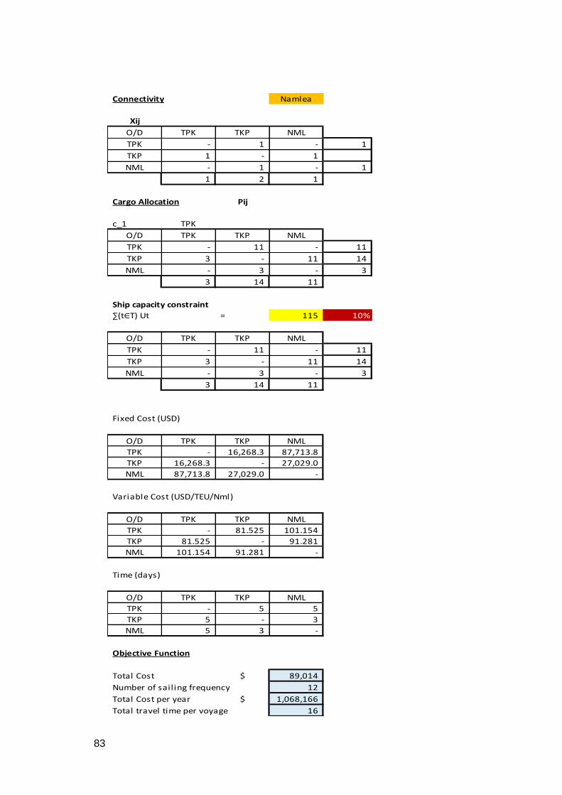
83
Connectivity Namlea
Xij
O/D TPK TKP NML
TPK - 1 - 1
TKP 1 - 1
NML - 1 - 1
1 2 1
Cargo Allocation Pij
c_1 TPK
O/D TPK TKP NML
TPK - 11 - 11
TKP 3 - 11 14
NML - 3 - 3
3 14 11
Ship capacity constraint
∑(t∈T) Ut = 115 10%
O/D TPK TKP NML
TPK - 11 - 11
TKP 3 - 11 14
NML - 3 - 3
3 14 11
Fixed Cost (USD)
O/D TPK TKP NML
TPK - 16,268.3 87,713.8
TKP 16,268.3 - 27,029.0
NML 87,713.8 27,029.0 -
Variable Cost (USD/TEU/Nml)
O/D TPK TKP NML
TPK - 81.525 101.154
TKP 81.525 - 91.281
NML 101.154 91.281 -
Time (days)
O/D TPK TKP NML
TPK - 5 5
TKP 5 - 3
NML 5 3 -
Objective Function
Total Cost $ 89,014
Number of sail ing frequency 12
Total Cost per year $ 1,068,166
Total travel time per voyage 16

84
Connectivity Fak-Fak
Xij
O/D TPK TKP FAK
TPK - 1 - 1
TKP 1 - 1
FAK - 1 - 1
1 2 1
Cargo Allocation Pij
c_1 TPK
O/D TPK TKP FAK
TPK - 106 - 106
TKP 10 - 106 116
FAK - 10 - 10
10 116 106
Ship capacity constraint
∑(t∈T) Ut = 115 92%
O/D TPK TKP FAK
TPK - 106 - 106
TKP 10 - 106 116
FAK - 10 - 10
10 116 106
Fixed Cost (USD)
O/D TPK TKP FAK
TPK - 16,268.3 116,672.0
TKP 16,268.3 - 45,040.0
FAK 116,672.0 45,040.0 -
Variable Cost (USD/TEU/Nml)
O/D TPK TKP FAK
TPK - 81.525 92.116
TKP 81.525 - 89.209
FAK 92.116 89.209 -
Time (days)
O/D TPK TKP FAK
TPK - 5 6
TKP 5 - 4
FAK 6 4 -
Objective Function
Total Cost $ 142,422
Number of sail ing frequency 12
Total Cost per year $ 1,709,060
Total travel time per voyage 18

85
Connectivity Kaimana
Xij
O/D TPK TKP KMN
TPK - 1 - 1
TKP 1 - 1
KMN - 1 - 1
1 2 1
Cargo Allocation Pij
c_1 TPK
O/D TPK TKP KMN
TPK - 114 - 114
TKP 7 - 114 121
KMN - 7 - 7
7 121 114
Ship capacity constraint
∑(t∈T) Ut = 135 84%
O/D TPK TKP KMN
TPK - 114 - 114
TKP 7 - 114 121
KMN - 7 - 7
7 121 114
Fixed Cost (USD)
O/D TPK TKP KMN
TPK - 16,268.3 137,552.4
TKP 16,268.3 - 43,437.6
KMN 137,552.4 43,437.6 -
Variable Cost (USD/TEU/Nml)
O/D TPK TKP KMN
TPK - 81.525 111.833
TKP 81.525 - 106.438
KMN 111.833 106.438 -
Time (days)
O/D TPK TKP KMN
TPK - 5 7
TKP 5 - 4
KMN 7 4 -
Objective Function
Total Cost $ 142,155
Number of sail ing frequency 12
Total Cost per year $ 1,705,864
Total travel time per voyage 18

86
Connectivity Timika
Xij
O/D TPK TKP TMK
TPK - 1 1
TKP 1 1
TMK 1 1
1 2 1
Cargo Allocation Pij
c_1 TPK
O/D TPK TKP TMK
TPK - 157 - 157
TKP 8 - 157 165
TMK - 8 - 8
8 165 157
∑(t∈T) Ut = 200 79%
O/D TPK TKP TMK
TPK - 157 - 157
TKP 8 - 157 165
TMK - 8 - 8
8 165 157
Fixed Cost (USD)
O/D TPK TKP TMK
TPK - 16,268.3 161,829.8
TKP 16,268.3 - 84,841.7
TMK 161,829.8 84,841.7 -
Variable Cost (USD/TEU/Nml)
O/D TPK TKP TMK
TPK - 81.525 111.833
TKP 81.525 - 119.693
TMK 111.833 119.693 -
Time (days)
O/D TPK TKP TMK
TPK - 5 8
TKP 5 - 5
TMK 8 5 -
Objective Function
Total Cost $ 235,421
Number of sail ing frequency 36
Total Cost per year $ 8,475,156
Total travel time per voyage 20

87
Connectivity Saumlaki
Xij
O/D TPK TKP SML
TPK - 1 1
TKP 1 1
SML 1 1
1 2 1
Cargo Allocation Pij
c_1 TPK
O/D TPK TKP SML
TPK - 11 - 11
TKP 1 - 11 12
SML - 1 - 1
1 12 11
∑(t∈T) Ut = 115 10%
O/D TPK TKP SML
TPK - 11 - 11
TKP 1 - 11 12
SML - 1 - 1
1 12 11
Fixed Cost (USD)
O/D TPK TKP SML
TPK - 16,268.3 121,361.6
TKP 16,268.3 - 27,468.6
SML 121,361.6 27,468.6 -
Variable Cost (USD/TEU/Nml)
O/D TPK TKP SML
TPK - 81.525 111.454
TKP 81.525 - 100.081
SML 111.454 100.081 -
Time (days)
O/D TPK TKP SML
TPK - 5 6
TKP 5 - 3
SML 6 3 -
Objective Function
Total Cost $ 89,653
Number of sail ing frequency 12
Total Cost per year $ 1,075,838
Total travel time per voyage 16

88
Connectivity Kalabahi
Xij
O/D TPK TKP KLB
TPK - 1 1
TKP 1 1
KLB 1 1
1 2 1
Cargo Allocation Pij
c_1 TPK
O/D TPK TKP KLB
TPK - 92 - 92
TKP 9 - 92 101
KLB - 9 - 9
9 101 92
∑(t∈T) Ut = 135 68%
O/D TPK TKP KLB
TPK - 92 - 92
TKP 9 - 92 101
KLB - 9 - 9
9 101 92
Fixed Cost (USD)
O/D TPK TKP KLB
TPK - 16,268.3 71,498.6
TKP 16,268.3 - 11,315.7
KLB 71,498.6 11,315.7 -
Variable Cost (USD/TEU/Nml)
O/D TPK TKP KLB
TPK - 81.525 81.496
TKP 81.525 - 78.942
KLB 81.496 78.942 -
Time (days)
O/D TPK TKP KLB
TPK - 5 4
TKP 5 - 2
KLB 4 2 -
Objective Function
Total Cost $ 71,375
Number of sail ing frequency 12
Total Cost per year $ 856,503
Total travel time per voyage 14

89
Connectivity Moa
Xij
O/D TPK TKP MOA
TPK - 1 1
TKP 1 1
MOA 1 1
1 2 1
Cargo Allocation Pij
c_1 TPK
O/D TPK TKP MOA
TPK - 11 - 11
TKP 1 - 11 12
MOA - 1 - 1
1 12 11
∑(t∈T) Ut = 115 10%
O/D TPK TKP MOA
TPK - 11 - 11
TKP 1 - 11 12
MOA - 1 - 1
1 12 11
Fixed Cost (USD)
O/D TPK TKP MOA
TPK - 16,268.3 96,645.2
TKP 16,268.3 - 27,468.6
MOA 96,645.2 27,468.6 -
Variable Cost (USD/TEU/Nml)
O/D TPK TKP MOA
TPK - 81.525 102.654
TKP 81.525 - 91.281
MOA 102.654 91.281 -
Time (days)
O/D TPK TKP MOA
TPK - 5 5
TKP 5 - 3
MOA 5 3 -
Objective Function
Total Cost $ 89,548
Number of sail ing frequency 12
Total Cost per year $ 1,074,570
Total travel time per voyage 16

90
Connectivity Dobo
Xij
O/D TPK TKP DBO
TPK - 1 - 1
TKP 1 - 1 2
DBO - 1 - 1
1 2 1
1 2 1
Cargo Allocation Pij
c_1 TPK
O/D TPK TKP DBO
TPK - 101 - 101
TKP 21 - 91 112
DBO - 21 - 21
21 122 91
∑(t∈T) Ut = 115 88%
O/D TPK TKP DBO
TPK - 101 - 101
TKP 21 - 91 112
DBO - 21 - 21
21 122 91
Fixed Cost (USD)
O/D TPK TKP DBO
TPK - 16,268.3 120,334.2
TKP 16,268.3 - 27,468.6
DBO 120,334.2 27,468.6 -
Variable Cost (USD/TEU/Nml)
O/D TPK TKP DBO
TPK - 81.525 113.144
TKP 81.525 - 101.960
DBO 113.144 101.960 -
Time (days)
O/D TPK TKP DBO
TPK - 5 7
TKP 5 - 3
DBO 7 3 -
Objective Function
Total Cost $ 108,839
Number of sail ing frequency 12
Total Cost per year $ 1,306,072
Total travel time per voyage 16

91
Connectivity Merauke
Xij
O/D TPK TKP MRK
TPK - 1 - 1
TKP 1 - 1 2
MRK - 1 - 1
1 2 1
1 2 1
Cargo Allocation Pij
c_1 TPK
O/D TPK TKP MRK
TPK - 192 - 192
TKP 41 - 192 233
MRK - 41 - 41
41 233 192
∑(t∈T) Ut = 200 96%
O/D TPK TKP MRK
TPK - 192 - 192
TKP 41 - 192 233
MRK - 41 - 41
41 233 192
Fixed Cost (USD)
O/D TPK TKP MRK
TPK - 16,268.3 171,312.2
TKP 16,268.3 - 100,186.5
MRK 171,312.2 100,186.5 -
Variable Cost (USD/TEU/Nml)
O/D TPK TKP MRK
TPK - 81.525 90.100
TKP 81.525 - 96.566
MRK 90.100 96.566 -
Time (days)
O/D TPK TKP MRK
TPK - 5 9
TKP 5 - 5
MRK 9 5 -
Objective Function
Total Cost $ 274,405
Number of sail ing frequency 36
Total Cost per year $ 9,878,574
Total travel time per voyage 20

92
Connectivity Larantuka
Xij
O/D TPK TKP LRK
TPK - 1 - 1
TKP 1 - 1 2
LRK - 1 - 1
1 2 1
1 2 1
Cargo Allocation Pij
c_1 TPK
O/D TPK TKP LRK
TPK - 34 - 34
TKP 6 - 34 40
LRK - 6 - 6
6 40 34
∑(t∈T) Ut = 115 30%
O/D TPK TKP LRK
TPK - 34 - 34
TKP 6 - 34 40
LRK - 6 - 6
6 40 34
Fixed Cost (USD)
O/D TPK TKP LRK
TPK - 16,268.3 42,921.2
TKP 16,268.3 - 6,022.9
LRK 42,921.2 6,022.9 -
Variable Cost (USD/TEU/Nml)
O/D TPK TKP LRK
TPK - 81.525 84.675
TKP 81.525 - 86.324
LRK 84.675 86.324 -
Time (days)
O/D TPK TKP LRK
TPK - 5 4
TKP 5 - 1
LRK 4 1 -
Objective Function
Total Cost $ 51,296
Number of sail ing frequency 12
Total Cost per year $ 615,557
Total travel time per voyage 12

93
Connectivity Lewoleba
Xij
O/D TPK TKP LWB
TPK - 1 - 1
TKP 1 - 1 2
LWB - 1 - 1
1 2 1
1 2 1
Cargo Allocation Pij
c_1
O/D TPK TKP LWB
TPK - 20 - 20
TKP 6 - 20 26
LWB - 6 - 6
6 26 20
∑(t∈T) Ut = 115 17%
O/D TPK TKP LWB
TPK - 20 - 20
TKP 6 - 20 26
LWB - 6 - 6
6 26 20
Fixed Cost (USD)
O/D TPK TKP LWB
TPK - 16,268.3 49,708.0
TKP 16,268.3 - 4,805.4
LWB 49,708.0 4,805.4 -
Variable Cost (USD/TEU/Nml)
O/D TPK TKP LWB
TPK - 81.525 84.675
TKP 81.525 - 86.324
LWB 84.675 86.324 -
Time (days)
O/D TPK TKP LWB
TPK - 5 4
TKP 5 - 1
LWB 4 1 -
Objective Function
Total Cost $ 46,512
Number of sail ing frequency 12
Total Cost per year $ 558,138
Total travel time per voyage 12

94
Connectivity Rote
Xij
O/D TPK TKP RTE
TPK - 1 - 1
TKP 1 - 1 2
RTE - 1 - 1
1 2 1
1 2 1
Cargo Allocation Pij
c_1
O/D TPK TKP RTE
TPK - 2 - 2
TKP 1 - 2 3
RTE - 1 - 1
1 3 2
∑(t∈T) Ut = 115 2%
O/D TPK TKP RTE
TPK - 2 - 2
TKP 1 - 2 3
RTE - 1 - 1
1 3 2
Fixed Cost (USD)
O/D TPK TKP RTE
TPK - 16,268.3 51,274.2
TKP 16,268.3 - 4,805.4
RTE 51,274.2 4,805.4 -
Variable Cost (USD/TEU/Nml)
O/D TPK TKP RTE
TPK - 81.525 74.640
TKP 81.525 - 76.290
RTE 74.640 76.290 -
Time (days)
O/D TPK TKP RTE
TPK - 5 4
TKP 5 - 1
RTE 4 1 -
Objective Function
Total Cost $ 42,621
Number of sail ing frequency 12
Total Cost per year $ 511,451
Total travel time per voyage 12

95
Connectivity Sabu
Xij
O/D TPK TKP SBU
TPK - 1 - 1
TKP 1 - 1 2
SBU - 1 - 1
1 2 1
1 2 1
Cargo Allocation Pij
c_1
O/D TPK TKP SBU
TPK - 11 - 11
TKP 1 - 11 12
SBU - 1 - 1
1 12 11
∑(t∈T) Ut = 115 10%
O/D TPK TKP SBU
TPK - 11 - 11
TKP 1 - 11 12
SBU - 1 - 1
1 12 11
Fixed Cost (USD)
O/D TPK TKP SBU
TPK - 16,268.3 60,093.9
TKP 16,268.3 - 5,211.2
SBU 60,093.9 5,211.2 -
Variable Cost (USD/TEU/Nml)
O/D TPK TKP SBU
TPK - 81.525 74.640
TKP 81.525 - 76.290
SBU 74.640 76.290 -
Time (days)
O/D TPK TKP SBU
TPK - 5 5
TKP 5 - 1
SBU 5 1 -
Objective Function
Total Cost $ 44,853
Number of sail ing frequency 12
Total Cost per year $ 538,235
Total travel time per voyage 12

96
Connectivity Waingapu
Xij
O/D TPK TKP WGP
TPK - 1 - 1
TKP 1 - 1 2
WGP - 1 - 1
1 2 1
1 2 1
Cargo Allocation Pij
c_1
O/D TPK TKP WGP
TPK - 145 - 145
TKP 23 - 145 168
WGP - 23 - 23
23 168 145
∑(t∈T) Ut = 192 76%
O/D TPK TKP WGP
TPK - 145 - 145
TKP 23 - 145 168
WGP - 23 - 23
23 168 145
Fixed Cost (USD)
O/D TPK TKP WGP
TPK - 16,268.3 65,507.9
TKP 16,268.3 - 24,083.1
WGP 65,507.9 24,083.1 -
Variable Cost (USD/TEU/Nml)
O/D TPK TKP WGP
TPK - - 73.267
TKP - - 87.282
WGP 73.267 87.282 -
Time (days)
O/D TPK TKP WGP
TPK - 5 5
TKP 5 - 3
WGP 5 3 -
Objective Function
Total Cost $ 95,366
Number of sail ing frequency 12
Total Cost per year $ 1,144,394
Total travel time per voyage 16
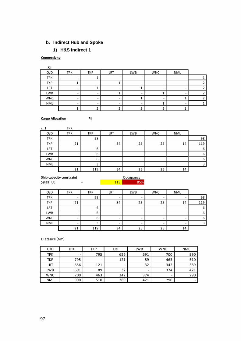
97
b. Indirect Hub and Spoke
1) H&S Indirect 1
Connectivity
Xij
O/D TPK TKP LRT LWB WNC NML
TPK - 1 - - - - 1
TKP 1 - 1 - - - 2
LRT - 1 - 1 - - 2
LWB - - 1 - 1 - 2
WNC - - - 1 - 1 2
NML - - - - 1 - 1
1 2 2 2 2 1
Cargo Allocation Pij
c_1 TPK
O/D TPK TKP LRT LWB WNC NML
TPK 98 98
TKP 21 34 25 25 14 119
LRT 6 6
LWB 6 6
WNC 6 6
NML 3 3
21 119 34 25 25 14
Ship capacity constraint Occupancy
∑(t∈T) Ut = 115 85%
O/D TPK TKP LRT LWB WNC NML
TPK - 98 - - - - 98
TKP 21 - 34 25 25 14 119
LRT - 6 - - - - 6
LWB - 6 - - - - 6
WNC - 6 - - - - 6
NML - 3 - - - - 3
21 119 34 25 25 14
O/D TPK TKP LRT LWB WNC NML
TPK - 795 656 691 700 990
TKP 795 - 121 89 463 510
LRT 656 121 - 32 342 389
LWB 691 89 32 - 374 421
WNC 700 463 342 374 - 290 NML 990 510 389 421 290 -
Distance (Nm)

98
Fixed Cost (USD)
O/D TPK TKP LRT LWB WNC NML
TPK - 16,268.32 42,921.17 49,708.00 62,473.54 87,713.82
TKP 16,268.32 - 6,022.91 4,805.40 25,270.32 27,028.95
LRT 42,921.17 6,022.91 - 3,307.80 16,536.05 21,853.37
LWB 49,708.00 4,805.40 3,307.80 - 6,554.54 15,084.22
WNC 62,473.54 25,270.32 16,536.05 6,554.54 - 24,692.67
Variable Cost (USD/TEU/Nml)
O/D TPK TKP LRT LWB WNC NML
TPK - 81.52 84.67 84.67 101.15 101.15
TKP 81.52 - 86.32 86.32 91.28 91.28
LRT 84.67 86.32 - 67.90 57.87 67.68
LWB 84.67 86.32 67.90 - 57.87 67.68
WNC 101.15 91.28 57.87 57.87 - 78.62
Time (days)
O/D TPK TKP LRT LWB WNC NML
TPK - 5 4 4 4 5
TKP 5 - 1 1 3 3
LRT 4 1 - 1 2 3
LWB 4 1 1 - 2 2
WNC 4 3 2 2 - 2
Objective Function
Total Cost $ 133,904
Number of sail ing frequency 12
Total Cost per year $ 1,606,853
Total travel time per voyage 22

99
2) H&S Indirect 2
Connectivity
Xij
O/D TPK TKP KLB MOA SML
TPK - 1 - - - 1
TKP 1 - 1 - - 2
KLB - 1 - 1 - 2
MOA - - 1 - 1 2
SML 1 1
1 2 2 2 1
Cargo Allocation Pij
c_1 TPK
O/D TPK TKP KLB MOA SML
TPK 140 140
TKP 11 112 14 14 151
KLB 9 - 9
MOA 1 - - 1
SML 1 - 1
11 151 112 14 14
Ship capacity constraint Occupancy
∑(t∈T) Ut = 192 73%
O/D TPK TKP KLB MOA SML
TPK - 140 - - - 140
TKP 11 - 112 14 14 151
KLB - 9 - - - 9
MOA - 1 - - - 1
SML - 1 - - - 1
11 151 112 14 14
O/D TPK TKP KLB MOA SML
TPK - 795 731 963 1,187
TKP 795 - 138 516 516
KLB 731 138 - 232 456
MOA 963 516 232 - 224
SML 1,187 516 456 224 -
Distance (Nm)

100
Fixed Cost (USD)
O/D TPK TKP KLB MOA SML
TPK - 16,268.32 61,720.34 83,138.48 104,202.62
TKP 16,268.32 - 11,315.72 27,468.61 27,468.61
KLB 61,720.34 11,315.72 - 20,785.93 38,638.93
MOA 83,138.48 27,468.61 20,785.93 - 20,161.85
SML 104,202.62 27,468.61 38,638.93 20,161.85 -
Variable Cost (USD/TEU/Nml)
O/D TPK TKP KLB MOA SML
TPK - 81.52 81.37 102.46 111.27
TKP 81.52 - 78.94 91.28 100.08
KLB 81.37 78.94 - 79.28 88.08
MOA 102.46 91.28 79.28 - 88.08
SML 111.27 100.08 88.08 88.08 -
Time (days)
O/D TPK TKP KLB MOA SML
TPK - 5 4 5 6
TKP 5 - 4 5 6
KLB 4 4 - 2 3
MOA 5 5 2 - 2
SML 6 6 3 2 -
Objective Function
Total Cost $ 161,796
Number of sail ing frequency 12
Total Cost per year $ 1,941,555
Total travel time per voyage 26

101
3) H&S Indirect 3
Connectivity
Xij
O/D TPK TKP RTE SBU WGP
TPK - 1 - - - 1
TKP 1 - 1 - - 2
RTE - 1 - 1 - 2
SBU - - 1 - 1 2
WGP 1 1
1 2 2 2 1
Cargo Allocation Pij
c_1 TPK
O/D TPK TKP RTE SBU WGP
TPK 162 162
TKP 25 3 14 145 187
RTE 1 - 1
SBU 1 - - 1
WGP 23 - 23
25 187 3 14 145
Ship capacity constraint Occupancy
∑(t∈T) Ut = 192 84%
O/D TPK TKP RTE SBU WGP
TPK - 162 - - - 162
TKP 25 - 3 14 145 187
RTE - 1 - - - 1
SBU - 1 - - - 1
WGP - 23 - - - 23
25 187 3 14 145
O/D TPK TKP RTE SBU WGP
TPK - 795 840 920 1,039
TKP 795 - 89 104 279
RTE 840 89 - 80 199
SBU 920 104 80 - 119
WGP 1,039 279 199 119 -
Distance (Nm)

102
Fixed Cost (USD)
O/D TPK TKP RTE SBU WGP
TPK - 16,268.32 51,274.19 60,093.90 65,507.90
TKP 16,268.32 - 4,805.40 5,211.24 24,083.08
RTE 51,274.19 4,805.40 - 5,160.71 13,632.38
SBU 60,093.90 5,211.24 5,160.71 - 7,020.26
WGP 65,507.90 24,083.08 13,632.38 7,020.26 -
Variable Cost (USD/TEU/Nml)
O/D TPK TKP RTE SBU WGP
TPK - 81.52 74.64 74.64 73.27
TKP 81.52 - 76.29 76.29 87.28
RTE 74.64 76.29 - 57.87 67.68
SBU 74.64 76.29 57.87 - 67.68
WGP 73.27 87.28 67.68 67.68 -
Time (days)
O/D TPK TKP RTE SBU WGP
TPK - 5 4 5 5
TKP 5 - 1 1 2
RTE 4 1 - 1 2
SBU 5 1 1 - 2
WGP 5 2 2 2 -
Objective Function
Total Cost $ 97,867
Number of sail ing frequency 12
Total Cost per year $ 1,174,409
Total travel time per voyage 18

103
Appendix 5. Regression Formula
1. DWT – Main Engine (ME)
2. DWT – Auxaliary Engine (AE)
y = 0,6475x + 446,14R² = 0,9851
0
10000
20000
30000
40000
50000
60000
70000
80000
0 20000 40000 60000 80000 100000 120000
DWT - Main Engine
y = 0,1384x + 645,53R² = 0,9292
0
2000
4000
6000
8000
10000
12000
14000
16000
18000
20000
0 20000 40000 60000 80000 100000 120000 140000
DWT-AE
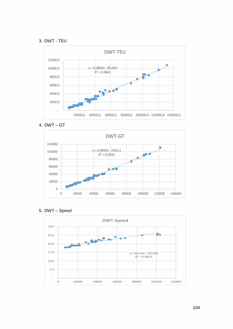
104
3. DWT - TEU
4. DWT – GT
5. DWT – Speed
y = 0,0804x - 80,693R² = 0,9841
-
2000,0
4000,0
6000,0
8000,0
10000,0
12000,0
- 20000,0 40000,0 60000,0 80000,0 100000,0 120000,0 140000,0
DWT-TEU
y = 0,9005x - 2433,1R² = 0,9924
0
20000
40000
60000
80000
100000
120000
0 20000 40000 60000 80000 100000 120000 140000
DWT-GT

105
Appendix 6. Cost Comparison
The RouteName of
the Port
Ship's
Capacity
(Teu)
Number of
ships
needed
per month
Number of
Sailing
Frequency
per year
Traveling
time
(days)
Utilizati-
on of
vessel
Total Shipping
Cost per route
N-1 192 4 48 26 95% 15,797,353$
N-2 199 4 48 26 98% 16,995,622$
N-3 135 2 24 14 79% 2,167,448$
34,960,423$
N-1 115 1 12 12 28% 1,347,655$
N-13 192 4 48 20 91% 15,112,078$
N-2 200 1 12 16 57% 2,963,685$
N-11 199 4 48 20 84% 16,486,649$
N-3 135 2 24 14 79% 2,167,448$
38,077,514$
H&S 1 Wanci 115 1 12 16 18% 1,052,916$
H&S 2 Namlea 115 1 12 16 10% 1,068,166$
H&S 3 Fak-Fak 115 1 12 18 92% 1,709,060$
H&S 4 Kaimana 135 1 12 18 84% 1,705,864$
H&S 5 Timika 200 3 36 20 79% 8,475,156$
H&S 6 Saumlaki 115 1 12 16 10% 1,075,838$
H&S 7 Kalabahi 135 1 12 14 68% 856,503$
H&S 8 Moa 115 1 12 16 10% 1,074,570$
H&S 9 Dobo 115 1 12 16 88% 1,306,072$
H&S 10 Merauke 200 3 36 20 96% 9,878,574$
H&S 11 Larantuka 115 1 12 12 30% 615,557$
H&S 12 Lewoleba 115 1 12 12 17% 558,138$
H&S 13 Rote 115 1 12 12 2% 511,451$
H&S 14 Sabu 115 1 12 12 10% 538,235$
H&S 15 Waingapu 192 1 12 16 76% 1,144,394$
31,570,494$
Total Shipping Cost
Total Shipping cost
Total Shipping cost
The RouteName of
the Port
Ship's
Capacity
(Teu)
Number of
ships
needed
Number of
Sailing
Frequency
per year
Traveling
time
(days)
Utilizati-
on of
vessel
Total Shipping
Cost per route
115 1 12 22 85% 1,606,853$
192 1 12 26 73% 1,941,555$
192 1 12 18 84% 1,174,409$
H&S 3 Fak-Fak 115 1 12 18 92% 1,709,060$
H&S 4 Kaimana 135 1 12 18 84% 1,705,864$
H&S 5 Timika 200 3 36 20 79% 8,475,156$
H&S 9 Dobo 115 1 12 16 88% 1,306,072$
H&S 10 Merauke 200 3 36 20 96% 9,878,574$
27,797,543$
H&S Indirect 1
H&S Indirect 2
H&S Indirect 3
Total Shipping cost