analog computation by dna strand displacement circuitsreif/paper/tianqi/analogdna/analogdna.pdf ·...

Analog Computation by DNA Strand Displacement

Circuits

Tianqi Song, Sudhanshu Garg, Reem Mokhtar, Hieu Bui, and John Reif∗

Department of Computer Science, Duke University,

Durham, NC, 27705, USA

E-mail: [email protected]

Abstract

DNA circuits have been widely used to develop biological computing devices because of their

high programmability and versatility. Here, we propose an architecture for the systematic

construction of DNA circuits for analog computation based on DNA strand displacement. The

elementary gates in our architecture include addition, subtraction, and multiplication gates.

The input and output of these gates are analog, which means that they are directly represented

by the concentrations of the input and output DNA strands respectively, without requiring a

threshold for converting to Boolean signals. We provide detailed domain designs and kinetic

simulations of the gates to demonstrate their expected performance. Based on these gates, we

describe how DNA circuits to compute polynomial functions of inputs can be built. Using

Taylor Series and Newton Iteration methods, functions beyond the scope of polynomials can

also be computed by DNA circuits built upon our architecture.

Keywords: DNA nanoscience, molecular programming, DNA computing, analog computa-

tion, self-assembly, DNA nanotechnology

∗To whom correspondence should be addressed

1

1 Introduction

1.1 Motivation

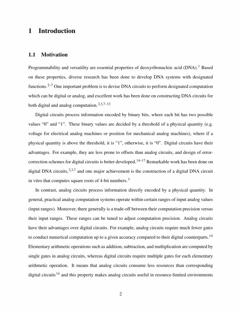
Programmability and versatility are essential properties of deoxyribonucleic acid (DNA).1 Based

on these properties, diverse research has been done to develop DNA systems with designated

functions.2–7 One important problem is to devise DNA circuits to perform designated computation

which can be digital or analog, and excellent work has been done on constructing DNA circuits for

both digital and analog computation.2,3,7–13

Digital circuits process information encoded by binary bits, where each bit has two possible

values “0” and “1”. These binary values are decided by a threshold of a physical quantity (e.g.

voltage for electrical analog machines or position for mechanical analog machines), where if a

physical quantity is above the threshold, it is “1”, otherwise, it is “0”. Digital circuits have their

advantages. For example, they are less prone to offsets than analog circuits, and design of error-

correction schemes for digital circuits is better developed.14–17 Remarkable work has been done on

digital DNA circuits,2,3,7 and one major achievement is the construction of a digital DNA circuit

in vitro that computes square roots of 4-bit numbers.3

In contrast, analog circuits process information directly encoded by a physical quantity. In

general, practical analog computation systems operate within certain ranges of input analog values

(input ranges). Moreover, there generally is a trade-off between their computation precision versus

their input ranges. These ranges can be tuned to adjust computation precision. Analog circuits

have their advantages over digital circuits. For example, analog circuits require much fewer gates

to conduct numerical computation up to a given accuracy compared to their digital counterparts.14

Elementary arithmetic operations such as addition, subtraction, and multiplication are computed by

single gates in analog circuits, whereas digital circuits require multiple gates for each elementary

arithmetic operation. It means that analog circuits consume less resources than corresponding

digital circuits14 and this property makes analog circuits useful in resource-limited environments

2

(e.g. in living cells18). Furthermore, for some applications, analog circuits can be more robust

than digital circuits.19 Excellent work has been done on inventing general schemes to implement

arbitrary chemical reaction networks (CRNs) with DNA strand displacement.10,13 Analog DNA

circuits with continuous dynamics (e.g. controllers, oscillators) have been developed based on

these schemes.8,9,11,12

1.2 Overview of Analog Computation

There is an extensive history of analog computation.20 In general, an analog computer has com-

ponents (arithmetic gates) that compute basic arithmetic operations such as addition, subtraction,

and multiplication. These operations may be done by various physical means, such as cog-based

mechanical devices or electrical circuits, etc. Typically, the range of values (e.g. the range of

mechanical positions in a mechanical analog computer or voltage range in an electrical analog

computer) computed by a given precision by an analog arithmetic gate is restricted, due to var-

ious physical constraints, but typically this is not a limitation, since the values can be scaled to

arbitrary ranges. Hence the precision of each arithmetic gate is ultimately limited by underlying

physical constraints on the devices that implement the arithmetic gate, but the precision can typi-

cally be tuned by adjusting the input ranges. All known analog computers (including in particular

our proposed DNA-based analog circuits) appear to have some sort of trade-off between precision

of analog values computed and the operating range of values over which the analog computations

are done. Analog devices can offer some advantages (such as requiring a smaller number of gates)

over computing devices whose gates can only execute Boolean operations. The same issues of

advantages (e.g., in number of gates) and limitations (e.g, in the range of values, but released via

rescaling) appear in the DNA-based analog circuits of this paper. Analog circuits for arithmetic

operations compute the outputs whose values are determined by the inputs. Analog circuits with

continuous dynamics generate outputs that are designated functions in the time domain.

3

1.3 Potential Applications of Analog DNA Circuits

Analog DNA circuits can be used as analog control devices11,12 where real values are sensed

and analog computation provides controlling output. For example, control of chemical reaction

networks requires both sensing of concentrations of input molecules and after analog computation,

controlling concentrations of output molecules. Also, in applications known as “DNA doctor”,21

where various nucleic acid sequence concentrations (e.g., concentrations of mRNAs) are sensed,

and an analog computation can be used to determine the amount of a drug molecule concentration

that should be released. Prior devices for control of chemical reaction networks and DNA doctor21

applications have been limited to finite-state control, and analog DNA circuits will allow much

more sophisticated analog signal processing and control. DNA robotics have allowed devices to

operate autonomously (e.g., to walk on a nanostructure) but also have been limited to finite-state

control. Analog DNA circuits can allow molecular robots to include real-time analog control

circuits to provide much more sophisticated control than offered by purely digital control. Many

artificial intelligence systems (e.g., neural networks and probabilistic inference) that dynamically

learn from environments require analog computation,14 and analog DNA circuits can be used for

back-propagation computation of neural networks and Bayesian probabilistic inference systems.

1.4 Prior Molecular-Scale Analog Computation

There is considerable excellent prior work on engineering nucleic acid systems8–12,22–24(both using

enzymes and enzyme-free) and cells18,25,26 to do complex dynamics. For example, the following

ingenious prior systems have been demonstrated to compute time-varying cyclic signals: (a) a nu-

cleic acid system using enzymes,22 (b) a DNA-based system using only hybridization reactions,8

(c) and a cell-based system.25 Prior work on analog DNA systems has mainly focused on develop-

ing DNA circuits with continuous dynamics.8,9,11,12 There is still a need to develop an architecture

to construct analog DNA circuits for arithmetic computation. In principle, the general schemes to

implement arbitrary chemical reaction networks (CRNs) with DNA strand displacement10,13 can

serve as such an architecture, but there needs to be more detailed investigation.

4

1.5 Our Contribution

In this paper, we present an architecture to construct DNA circuits for arithmetic computation in

an analog fashion. There are three elementary gates in out architecture: addition, subtraction and

multiplication gates. For each gate, we first propose its high-level chemical reaction network anal-

ogy and then give our DNA implementation. Each gate is evaluated by simulation using Language

for Biochemical Systems (LBS).27 DNA circuits to compute polynomial functions of inputs can be

built based on these gates. By Taylor Series and Newton Iteration methods, some functions beyond

the scope of polynomials can also be computed by DNA circuits built upon our architecture.

2 Results

2.1 Preliminaries of Analog DNA Gates

2.1.1 Toehold-mediated Strand Displacement

Figure 1: A domain-level illustration of toehold-mediated strand displacement. Reaction 1 is a reversible re-action, where the forward reaction and the reverse reaction are called toehold binding and toehold unbindingrespectively. Reaction 2 is called branch migration.

Toehold-mediated strand displacement is the primary mechanism for the proposed architecture. A

domain-level illustration of toehold-mediated strand displacement is shown in Figure 1. We call

the a∗ domain in G a toehold, where a domain is a sequence of nucleotides. The arrow in a DNA

strand indicates the 3′ end. In reaction 1, the a domain in I hybridizes to the a∗ domain in G, where

the asterisk symbol means complementary domain. We call this step toehold binding. Usually, the

5

toehold domain is short (less than 10 nucleotides), so the toehold binding reaction is reversible and

we call the reverse reaction toehold unbinding. Once the toehold binding step is complete, reaction

2 can happen where the x domain in I (called branch migration domain) competes with the sp5

strand in G on binding to the x∗ domain. Eventually, strand I wins and displaces sp5. We call this

step branch migration. In the diagrams of this paper, we combine these two steps into a single step

for simplicity.

2.1.2 Related Concepts

Here we introduce some basic concepts to define our analog DNA gates.

Input range: Each analog gate is assigned an input range, within which the inputs of a gate

should lie if they are to be computed within the required precision. Hence if one of the inputs of

an arithmetic gate is outside its input range, the arithmetic operation may not be computed within

the required precision. Specifically, in our DNA-based analog computation architecture, the input

range of an analog DNA gate is the range of concentration within which its input DNA strands

should occur, in order for the gate to operate correctly. The input ranges are not particular to

our analog DNA gates, and typically any analog gate has an input range. Our analog DNA gates

have the advantage that the input range can be tuned easily by programming the concentrations of

components in a gate.

Valid output range: Analog gates process continuous physical quantities as input and provide

continuous output. This makes analog gates suffer more from two things compared to digital gates:

signal fluctuation and signal degradation. Continuous information is more sensitive to noise and

more difficult to restore than discrete information encoded by binary bits. Therefore, due to noise,

the output of an analog gate cannot remain at the theoretically correct value for given inputs. There

will always be an error, which usually tends to grow larger over time due to signal degradation.

To evaluate analog gates, we define the term valid output range: Given inputs x1 and x2, a gate

that conducts arithmetic operation ⊗, and 0 < r < 1 which describes the error, the valid output

range is ((1− r) ∗ (x1⊗ x2),(1+ r) ∗ (x1⊗ x2)) for inputs x1 and x2. The output lying within this

6

range is considered correct. The time that the output stays within the valid output range is used to

quantify the performance of the gate under these inputs. The value of r does not really influence

the execution of a gate and it is just a parameter for interpreting the performance.

Note that all known analog systems, like electronic and mechanical analog systems, have re-

stricted input ranges. Fluctuation and degradation of output signal is also a common problem for all

known analog systems, which necessitates a valid output range. These properties are unavoidable

for all analog systems,14 not only for our DNA-based analog system.

2.2 Abstractions of the Gates

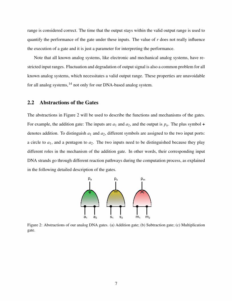
The abstractions in Figure 2 will be used to describe the functions and mechanisms of the gates.

For example, the addition gate: The inputs are a1 and a2, and the output is pa. The plus symbol +

denotes addition. To distinguish a1 and a2, different symbols are assigned to the two input ports:

a circle to a1, and a pentagon to a2. The two inputs need to be distinguished because they play

different roles in the mechanism of the addition gate. In other words, their corresponding input

DNA strands go through different reaction pathways during the computation process, as explained

in the following detailed description of the gates.

a1 a2

pa

s1 s2

ps pm

m1 m2

Figure 2: Abstractions of our analog DNA gates. (a) Addition gate; (b) Subtraction gate; (c) Multiplicationgate.

7

2.3 Addition Gate

2.3.1 The Chemical Reaction Network to Inspire Our Addition Gate

Our addition gate is inspired by the following chemical reaction network:

Ia1 +A1 k1−→ Oa (1a)

Ia2 +A2 k2−→ Oa (1b)

The addition gate computes pa = a1 +a2 (see abstraction in Figure 2) . Ia1 and Ia2 are input

chemical species to the gate, where their initial concentrations [Ia1]0, [Ia2]0 represent the two

inputs a1 and a2 respectively, which means a1 = [Ia1]0 and a2 = [Ia2]0. The addition gate is

composed of chemical species A1 and A2. To have an input range of (0,ra) which means a1,a2 ∈

(0,ra), we let the initial concentrations be [A1]0 = [A2]0 = ra. Oa is the output strand of this gate

and its concentration at equilibrium [Oa]∞ represents pa. As shown in reactions (1a) and (1b), all

Ia1 and Ia2 will eventually be transformed to Oa and then [Oa]∞ = [Ia1]0 +[Ia2]0 which means

pa = a1 +a2. There are no constraints on rate constants k1 and k2.

2.3.2 DNA Implementation of Our Addition Gate

As shown in Figure 3, Ia1 and Ia2 are two input DNA strands. Their initial concentrations [Ia1]0

and [Ia2]0 represent a1 and a2, respectively. Oa, which is the DNA strand composed of domains

y1-a-x3 (5′ to 3′ direction) is the output DNA strand and its concentration at equilibrium [Oa]∞

represents pa. Each of A1 and A2 is implemented by three DNA species, where a DNA species is

a DNA strand or complex. The DNA reactions in the addition gate are shown in Figures 4 and 5.

The relationship between the original chemical reaction network and DNA reactions is shown in

Table 1. The simulation to demonstrate this DNA implementation is in Section 2.7.

8

Figure 3: DNA design of our addition gate. Each of A1 and A2 in the original chemical reaction network isimplemented by three DNA species (e.g., A1 is implemented by Fa, Ga1 and Da1). Initial concentrationsare [Ga1]0=[Da1]0=[Ga2]0=[Da2]0 = ra, and [Fa]0 = 2ra because it is in both A1 and A2, where (0,ra) isthe input range. The grey domains are branch migration domains of 20 nucleotides in length. The colordomains are toeholds of 5 nucleotides in length. All DNA figures are drawn by Visual DSD28 in this paper.

Table 1: Each abstract chemical reaction is implemented by several DNA reactions. The DNA reactionscorresponding to the numbers are shown in Figures 4 and 5.

Abstract chemical reaction DNA reactions1a 1,2,3,41b 5,6,7,8

2.4 Subtraction Gate

2.4.1 The Chemical Reaction Network to Inspire Our Subtraction Gate

Our subtraction gate is inspired by the following chemical reaction network:

Is2 +S k1−→ S′

(2a)

Is1 +S′ k2−→ /0 (2b)

The subtraction gate computes ps = s1− s2, where s1 > s2 is required (see abstraction in Fig-

ure 2) . Is1 and Is2 are input chemical species to the gate, where their initial concentrations [Is1]0,

[Is2]0 represent the two inputs s1 and s2 respectively, which means s1 = [Is1]0 and s2 = [Is2]0.

The subtraction gate is composed of chemical species S. To have an input range of (0,rs) which

9

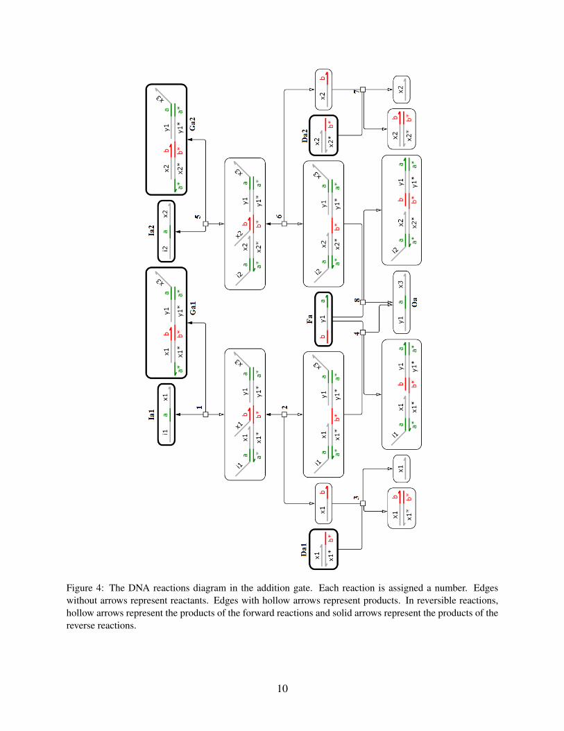
Figure 4: The DNA reactions diagram in the addition gate. Each reaction is assigned a number. Edgeswithout arrows represent reactants. Edges with hollow arrows represent products. In reversible reactions,hollow arrows represent the products of the forward reactions and solid arrows represent the products of thereverse reactions.

10

Figure 5: A list of the DNA reactions in the addition gate. Each reaction is assigned a number, which isconsistent with Figure 4. The rate constants in such lists in this paper are discussed in Section 4

means s1,s2 ∈ (0,rs), we let the initial concentrations be [S]0 = rs. S′ is intermediate product. The

concentration of Is1 at equilibrium [Is1]∞ represents ps. As shown in reactions (2a) and (2b), Is2

and Is1 cancel each other in pairs which leaves [Is1]∞ = [Is1]0− [Is2]0 concentration of Is1, and

then we have ps = s1− s2. If s1 ≤ s2, all Is1 will be consumed and the result is just 0. There are

no constraints on rate constants k1 and k2.

11

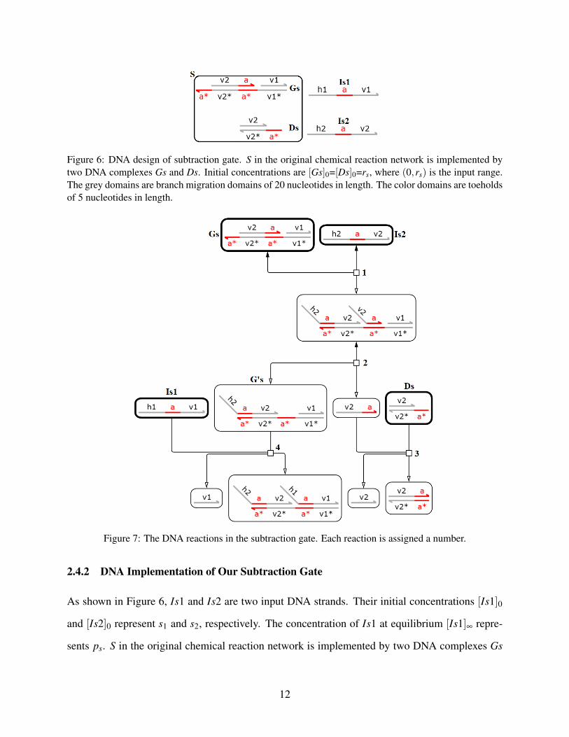
Figure 6: DNA design of subtraction gate. S in the original chemical reaction network is implemented bytwo DNA complexes Gs and Ds. Initial concentrations are [Gs]0=[Ds]0=rs, where (0,rs) is the input range.The grey domains are branch migration domains of 20 nucleotides in length. The color domains are toeholdsof 5 nucleotides in length.

Figure 7: The DNA reactions in the subtraction gate. Each reaction is assigned a number.

2.4.2 DNA Implementation of Our Subtraction Gate

As shown in Figure 6, Is1 and Is2 are two input DNA strands. Their initial concentrations [Is1]0

and [Is2]0 represent s1 and s2, respectively. The concentration of Is1 at equilibrium [Is1]∞ repre-

sents ps. S in the original chemical reaction network is implemented by two DNA complexes Gs

12

Figure 8: A list of the DNA reactions in the subtraction gate. Each reaction is assigned a number, which isconsistent with Figure 7.

and Ds. The DNA reactions in the subtraction gate are shown in Figures 7 and 8. The relation-

ship between the original chemical reaction network and DNA reactions is shown in Table 2. The

simulation to demonstrate this DNA implementation is in Section 2.7.

Table 2: Each abstract chemical reaction is implemented by one or several DNA reactions. The DNAreactions corresponding to the numbers are shown in Figures 7 and 8.

Abstract chemical reaction DNA reactions2a 1,2,32b 4

2.5 Multiplication Gate

2.5.1 The Chemical Reaction Network to Inspire Our Multiplication Gate

Our multiplication gate is inspired by the following chemical reaction network:

13

Im1 +M1 ks−→ Im1a (3a)

Im2 +M2k f−→ Im2a+ Im2b (3b)

Im2a+M3 k1−→ G′m3 (3c)

Im2b+Gm4 k2−→ /0 (3d)

Im1a+Gm4 k3−→ /0 (3e)

Im1a+G′m3 k3−→ Om1 (3f)

Om1 +Amplifier k4−→ Om+Om+ ..+Om︸︷︷︸rmOm

(3g)

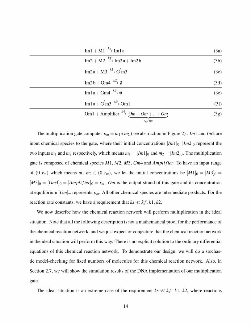
The multiplication gate computes pm = m1 ∗m2 (see abstraction in Figure 2) . Im1 and Im2 are

input chemical species to the gate, where their initial concentrations [Im1]0, [Im2]0 represent the

two inputs m1 and m2 respectively, which means m1 = [Im1]0 and m2 = [Im2]0. The multiplication

gate is composed of chemical species M1, M2, M3, Gm4 and Ampli f ier. To have an input range

of (0,rm) which means m1,m2 ∈ (0,rm), we let the initial concentrations be [M1]0 = [M3]0 =

[M3]0 = [Gm4]0 = [Ampli f ier]0 = rm. Om is the output strand of this gate and its concentration

at equilibrium [Om]∞ represents pm. All other chemical species are intermediate products. For the

reaction rate constants, we have a requirement that ks� k f , k1, k2.

We now describe how the chemical reaction network will perform multiplication in the ideal

situation. Note that all the following description is not a mathematical proof for the performance of

the chemical reaction network, and we just expect or conjecture that the chemical reaction network

in the ideal situation will perform this way. There is no explicit solution to the ordinary differential

equations of this chemical reaction network. To demonstrate our design, we will do a stochas-

tic model-checking for fixed numbers of molecules for this chemical reaction network. Also, in

Section 2.7, we will show the simulation results of the DNA implementation of our multiplication

gate.

The ideal situation is an extreme case of the requirement ks� k f , k1, k2, where reactions

14

(3b), (3c) and (3d) finish first, then reaction (3a) starts to produce Im1a, and then reactions (3e)

and (3f) start to work. It means that before reactions (3a), (3e) and (3f) start to work, reactions

(3b) , (3c) and (3d) have finished and made the concentration ratio between G′m3 and Gm4 be[G′m3][Gm4] =

[Im2]0rm−[Im2]0

= m2rm−m2

: Let the reaction volume be V . Reaction (3b) produces [Im2]0V amount

of Im2a, and then reaction (3c) produces [Im2]0V amount of G′m3. Reaction (3b) also produces

[Im2]0V amount of Im2b, and then reaction (3d) consumes [Im2]0V amount of Gm4, which means

that [Gm4]0V − [Im2]0V amount of Gm4 is left. Therefore, the concentration ratio between G′m3

and Gm4 will be [Im2]0V[Gm4]0V−[Im2]0V = m2

rm−m2.

Given that reactions (3e) and (3f) have the same rate constant, we expect that the Im1a produced

by reactions (3a) will be distributed to reactions (3e) and (3f) according to the concentration ratio

between G′m3 and Gm4 that we calculated above. This means that m2m2+(rm−m2)

portion of Im1a

will be consumed by reaction (3f) and then the concentration of Om1 at equilibrium is [Om1]∞ =

m1m2

m2+(rm−m2)= m1m2

rmif we ignore reaction (3g). By adding an amplification reaction (3g), we

have the concentration of Om at equilibrium be [Om]∞ = rmm1m2

rm= m1m2 = [Im1]0[Im2]0, where

we use [Om]∞ to represent the output of our multiplication gate.

To support our design, we conducted a stochastic model-checking for fixed numbers of molecules

for the chemical reaction network in the ideal situation. To simplify the simulation, we ignore re-

actions (3b), (3c) and (3d) (also (3g)). Instead, we directly set up the concentration ratio [G′m3]0[Gm4]0

and check how Im1a is distributed between reactions (3e) and (3f). Here we use the same nota-

tion for the number of molecules as the notation for concentration. There is no constraint on the

relationship between ks and k3, and then we just let ks = k3 = 0.01 s−1. Note that in stochastic

simulation of chemical reaction networks, s−1 is the unit of rate constants in bimolecular reactions.

The simulation is done by Language for Biochemical Systems (LBS)27 in a beta version of Visual

GEC.29

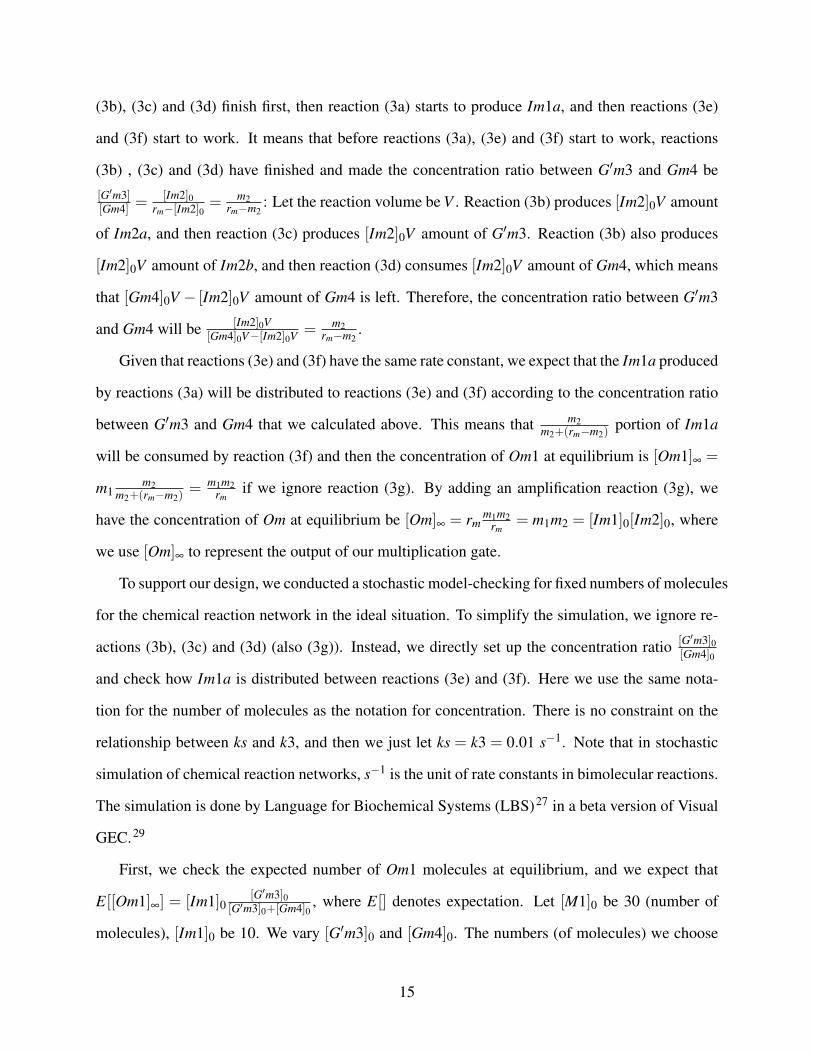
First, we check the expected number of Om1 molecules at equilibrium, and we expect that

E[[Om1]∞] = [Im1]0[G′m3]0

[G′m3]0+[Gm4]0, where E[] denotes expectation. Let [M1]0 be 30 (number of

molecules), [Im1]0 be 10. We vary [G′m3]0 and [Gm4]0. The numbers (of molecules) we choose

15

here do not have special meanings and it is just that we have to give specific numbers for stochastic

model check. To speed up the simulation, we choose small numbers. The simulation results are

shown in Table 3. In all cases, the results show that E[[Om1]∞] = [Im1]0[G′m3]0

[G′m3]0+[Gm4]0. We believe

that E[[Om1]∞] in this stochastic model is the value of [Om1]∞ in the deterministic model when

there are large number of molecules in the system.

Table 3: Simulation results for checking the expected number of Om1 molecules at equilibrium (E[[Om1]∞]).In all cases, the results show that E[[Om1]∞] = [Im1]0

[G′m3]0[G′m3]0+[Gm4]0

.

E[[Om1]∞] [G′m3]0 [Gm4]07.5 30 10

6.67 20 105 10 10

3.33 10 202.5 10 30

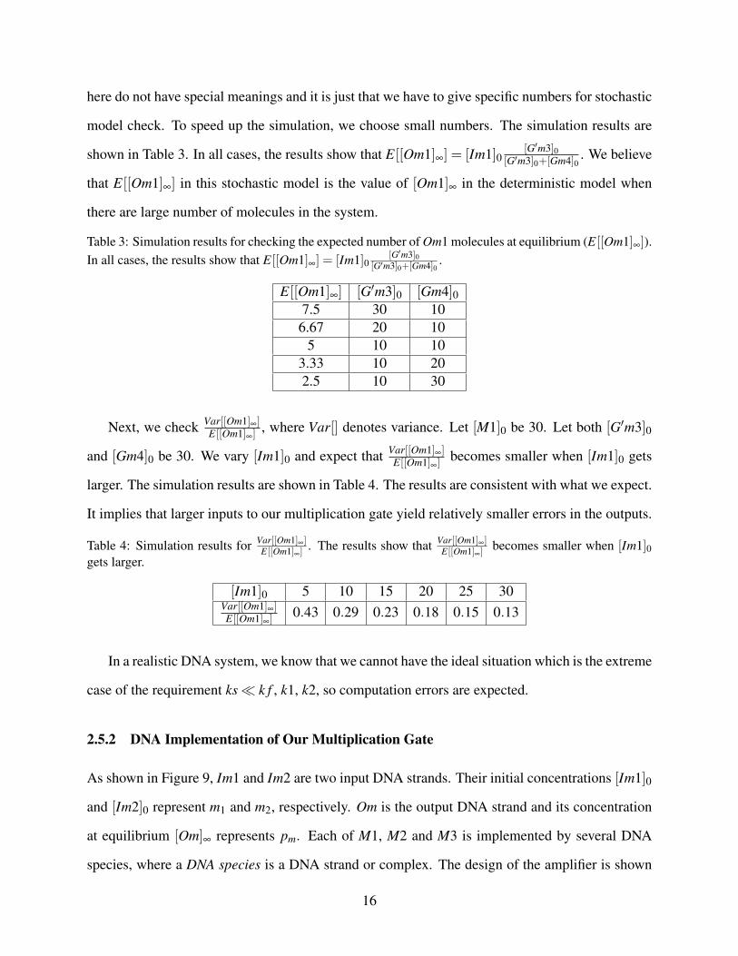
Next, we check Var[[Om1]∞]E[[Om1]∞]

, where Var[] denotes variance. Let [M1]0 be 30. Let both [G′m3]0

and [Gm4]0 be 30. We vary [Im1]0 and expect that Var[[Om1]∞]E[[Om1]∞]

becomes smaller when [Im1]0 gets

larger. The simulation results are shown in Table 4. The results are consistent with what we expect.

It implies that larger inputs to our multiplication gate yield relatively smaller errors in the outputs.

Table 4: Simulation results for Var[[Om1]∞]E[[Om1]∞]

. The results show that Var[[Om1]∞]E[[Om1]∞]

becomes smaller when [Im1]0gets larger.

[Im1]0 5 10 15 20 25 30Var[[Om1]∞]E[[Om1]∞]

0.43 0.29 0.23 0.18 0.15 0.13

In a realistic DNA system, we know that we cannot have the ideal situation which is the extreme

case of the requirement ks� k f , k1, k2, so computation errors are expected.

2.5.2 DNA Implementation of Our Multiplication Gate

As shown in Figure 9, Im1 and Im2 are two input DNA strands. Their initial concentrations [Im1]0

and [Im2]0 represent m1 and m2, respectively. Om is the output DNA strand and its concentration

at equilibrium [Om]∞ represents pm. Each of M1, M2 and M3 is implemented by several DNA

species, where a DNA species is a DNA strand or complex. The design of the amplifier is shown

16

Figure 9: DNA design of our multiplication gate. Each of M1, M2 and M3 in the original chemical reactionnetwork is implemented by several DNA species. Initial concentrations are [Fm1]0 = [Gm1]0 = [Dm1]0 =[Fm2]0 = [Gm2]0= [Gm3]0 = [Dm3]0 = [Gm4]0 = rm, where (0,rm) is the input range. The grey domainsare branch migration domains of 20 nucleotides in length. The color domains are toeholds of 5 nucleotidesin length.

in Figure 15. The DNA reactions in the multiplication gate are shown in Figures 10, 11, 12, 13,

and 14. The relationship between the original chemical reaction network and DNA reactions is

shown in Table 5.

To make reaction (3a) much slower than reactions (3b), (3c) and (3d) (ks� k f , k1, k2), we slow

down DNA reaction 3, where domain m2 of Fm1 is modified such that there are mismatches when

Fm1 displaces Im1a and then the toehold-mediated strand displacement is slowed down. In the

simulation of this paper, we let the strand displacement be slowed down by 2 orders of magnitude.

17

To make reactions (3e) and (3f) have the same rate constant, we let the two toehold-mediated strand

displacement reactions 11 and 12 have the same toehold g and branch migration domain n5-h (5′

to 3′ direction). The simulation to demonstrate this DNA implementation is in Section 2.7.

Table 5: Each abstract chemical reaction is implemented by one or several DNA reactions. The DNAreactions corresponding to the numbers are shown in Figures 10, 11, 12, 13, and 14.

Abstract chemical reaction DNA reactions3a 1,2,3,43b 5,6,73c 8,9,103d 113e 123f 13

2.5.3 Related Work on DNA Multiplication Gate

Zhang et al.30 proposed a DNA-based amplifier that has fixed gain. The concentration of the

product of their amplifier at equilibrium is αI0, where I0 is the initial concentration of the input

DNA strand and constant α is the gain of the amplifier. Genot et al.31 also developed a method

by which they can multiply a number (represented by the concentration of a DNA strand) by a

constant. Both their work is a preliminary step toward designing a multiplication gate. They can

multiply the input by a constant. The input is represented by the concentration of an input DNA

strand and the constant is encoded by the concentrations of the components of their amplifiers.

Lakin et al.32 developed a two-input multiplier but their multiplier is not autonomous, which means

that, in order to make the multiplier work as desired, the input DNA strands to the multiplier need

to be separately added into the solution manually at designated times.

2.6 Leak Reactions

Thus far, we have only described the designed reactions of the three gates. Here we discuss poten-

tial leak reactions (unintended reactions). As shown in Figure 17, the main leak reaction (reaction

1) in addition gate is caused by strand Fa, where Fa is able to displace Oa even in the absence of

18

Figure 10: The reactions in the multiplication gate. Each reaction is assigned a number.

19

Figure 11: A list of the DNA reactions in the multiplication gate (part1). Each reaction is assigned a number,which is consistent with Figure 10. Reaction 3 is slowed down by modifying domain m2 of Fm1 such thatthere are mismatches when Fm1 displaces Im1a.

Figure 12: A list of the DNA reactions in the multiplication gate (part2). Each reaction is assigned a number,which is consistent with Figure 10.

the input strand Ia1. This kind of leak reaction also happens between Ga2 and Fa in the addition

gate. The reason why this can happen is that the base pairs in the circled part of Ga1 can be tem-

porary broken and create a toehold for Fa. This kind of leak is typical in systems based on DNA

strand displacement. To reduce the leak, we can use some design techniques such as manipulat-

ing sequence design, incorporating clamps, etc.2–4,6,7,33–35 Both the subtraction and multiplication

gates suffer from the same leak mechanism. The leak (reaction 2) in the subtraction gate is that Is1

20



Figure 15: Design of a 2× amplifier, where one Om1 strand generates two Om strands. We can chooserm as a power of 2. For rm = 2n, we just need to connect n layers of such 2× amplifiers in series to get a2n× amplifier. The maximum possible input of layer-0 (represented by [Om1]) is rm∗rm

rm= rm = 2n as the

calculation in Section 2.5.1 with m1 = m2 = rm. Therefore, the maximum possible input of layer-i is 2n+i

(0 ≤ i ≤ n−1). In layer-i, we let the initial concentrations of the DNA strand Fi and the DNA complex Aibe 2n+i, such that the amplifier can afford the maximum possible input. The reactions in the amplifier areshown in Figure 16. The two Om strands are identical in terms that only the i-n7 (5′ to 3′ direction) part inthe two strands matters in further reactions.

21

Figure 16: The DNA reactions in a 2× amplifier.

can invade Gs and displace the v1 domain even if there is no Is2. The leak in the multiplication

gate is caused by strands Fm1 and Fm2 (reactions 3 and 4). In the amplifier of the multiplication

gate, there is also such leak (reaction 5).

The leak reactions will cause errors for the gates. As we said in the description of the gates,

we use the concentration of the output strand of a gate at equilibrium to represent the output of

this gate, if we do not consider leaks. If we want to evaluate the performance of a gate under

particular inputs, we just need to check the percentage difference between the output of the gate

(concentration of the output strand at equilibrium) and the theoretically correct result.

With leaks, we cannot use the concentration of the output strand at equilibrium to evaluate

the performance of a gate, because the leak reactions will keep generating output until it reaches

22

the maximum output value that a gate can provide. Instead, we use the time that the output stays

within the valid output range (see its definition in Section 2.1.2) to quantify the performance of a

gate under particular inputs. In this paper, we use r = 0.05 to define the valid output range (see the

meaning of r in Section 2.1.2).

Figure 17: The main leak reactions in our DNA gates: reaction 1 in the addition gate; reaction 2 in thesubtraction gate; reactions 3, 4, 5 in the multiplication gate.

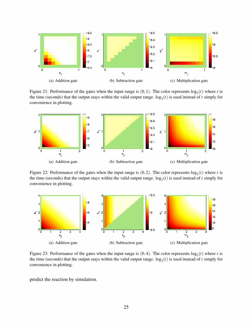
2.7 Simulation Results of the Gates

For each gate, we performed the simulation for three input ranges (0,1), (0,2) and (0,4). Later,

we will use gates within these input ranges to build analog DNA circuits to compute polynomials.

The model of simulation is discussed in Section 4.

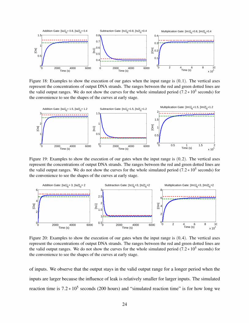
Figures 18, 19 and 20 shows an example for each gate for input ranges (0,1), (0,2), (0,4)

respectively, to give an intuitive sense of how our gates execute. The ranges between the red dotted

line and green dotted line are the valid output ranges. The output stays in the valid output range for

a long period in each case. The summary of the gates performance is shown in Figures 21, 22 and

23, and they show how long the output stays within the valid output range for each combination

23

0 2000 4000 60000

0.5

1

1.5

Time (s)

[Oa]

Addition Gate: [Ia1]0= 0.8, [Ia2]

0= 0.4

0 2000 4000 6000

0.4

0.5

0.6

0.7

0.8

Time (s)

[Is1]

Subtraction Gate: [Is1]0=0.8, [Is2]

0=0.4

0 2 4 6 8 10

x 105

0

0.1

0.2

0.3

0.4

Time (s)

[Om

]

Multiplication Gate: [Im1]0=0.8, [Im2]

0=0.4

Figure 18: Examples to show the execution of our gates when the input range is (0,1). The vertical axesrepresent the concentrations of output DNA strands. The ranges between the red and green dotted lines arethe valid output ranges. We do not show the curves for the whole simulated period (7.2 ∗ 105 seconds) forthe convenience to see the shapes of the curves at early stage.

0 2000 4000 60000

1

2

3

Time (s)

[Oa]

Addition Gate: [Ia1]0= 1.5, [Ia2]

0= 1.2

0 2000 4000 60000

0.5

1

1.5

Time (s)

[Is1]

Subtraction Gate: [Is1]0=1.5, [Is2]

0=1.2

0 0.5 1 1.5 2

x 105

0

0.5

1

1.5

2

Time (s)

[Om

]

Multiplication Gate: [Im1]0=1.5, [Im2]

0=1.2


0 2000 4000 60000

2

4

6

Time (s)

[Oa]

Addition Gate: [Ia1]0= 3, [Ia2]

0= 2

0 2000 4000 60000.5

1

1.5

2

2.5

3

Time (s)

[Is1]

Subtraction Gate: [Is1]0=3, [Is2]

0=2

0 2 4 6 8 10

x 104

0

2

4

6

8

Time (s)

[Om

]

Multiplication Gate: [Im1]0=3, [Im2]

0=2


of inputs. We observe that the output stays in the valid output range for a longer period when the

inputs are larger because the influence of leak is relatively smaller for larger inputs. The simulated

reaction time is 7.2 ∗ 105 seconds (200 hours) and “simulated reaction time” is for how long we

24

(a) Addition gate (b) Subtraction gate (c) Multiplication gate

Figure 21: Performance of the gates when the input range is (0,1). The color represents log2(t) where t isthe time (seconds) that the output stays within the valid output range. log2(t) is used instead of t simply forconvenience in plotting.





predict the reaction by simulation.

25

2.8 Strategy to Construct Analog DNA Circuits

Our analog gates are modular, which means that the input and output strands have the same motif.

This property confers scalability to circuits built by our gates. The simplest strategy of building

circuits is connecting the gates together by programming the branch migration domains’ sequences

in the output strands such that these strands can find their designated downstream gates. The

concern for this strategy is that when we designed and simulated the single gates, we assumed that

the inputs were “static” which means that they were fully prepared at the moment that the gates

started to work. However, when a gate is part of a circuit, its input may be “dynamic”, which means

that the inputs are dynamically (or gradually) produced by other gates, and this may influence the

performance of our gates.

This concern is common for all kinds of analog systems. Analog systems have the property

that they do not restore the signal for each stage and only the output signal is robust. We have

some methods to mitigate this problem in our architecture. The addition gate is not influenced

much by this issue because it is essentially just a transducer and it does not matter much how the

inputs arrive. For the subtraction gate, if either input comes earlier, it can simply wait for the

other one. Eventually, the cancellation between Is1 and Is2 will be finished, and the remaining Is1

will serve as output strands. For the multiplication gate, we make input strand Im2 be prepared

in a “static” fashion such that the desired concentration ratio between G′m3 and Gm4 is formed

as early as possible. Im1 can be prepared in a “dynamic” fashion by another gate, and this also

gives more time to the formation of the concentration ratio. For example, in Figure 25, for all

multiplication gates, the Im2 input strands (the input on the right) are prepared in a “static” fashion,

not dynamically (or gradually) produced by another gate.

Note that one issue for the subtraction gate is that input strand Is1 can skip this gate to react

with a downstream gate because Is1 serves both as input and output strands (e.g. in Figure 24).

This issue can be solved by using only one subtraction gate in a circuit and placing it at the output

port of the circuit (e.g. Figure 27), such that its output strand does not interact any downstream

gate. For example, a polynomial function f (x) = 3x4−2x3 +5x−1 can be transformed to f (x) =

26

(3x4 + 5x)− (2x3 + 1), which only has one subtraction operation. Since we require s1 > s2 in

our subtraction gate, circuits constructed by our architecture can only accept x such that f (x) =

(3x4 +5x)− (2x3 +1)> 0. This transformation does not increase the number of gates needed and

the only difference is that the circuit needs two subtraction gates and one addition gate for the

original polynomial, but it needs one subtraction gate and two addition gates for the transformed

polynomial.

Is1

Figure 24: The Is1 can skip gate-1 and go to gate-2.

In the following sections, we will first present the construction of analog DNA circuits to

compute polynomial functions of inputs. We show two examples: a circuit to compute f (x) =

1+ x+ x2

2! +x3

3! for 0 < x < 1, and a circuit to compute g(x,y) = 2y− y2x, for x,y ∈ (0,2) and

g(x,y) > 0. Then we use these two circuits to construct circuits that compute non-polynomial

functions by strategies such as Taylor Series and Newton Iteration.

2.9 An Analog DNA Circuit to Compute f (x) = 1+ x+ x2

2! +x3

3! for 0 < x < 1

Figure 25 shows an analog DNA circuit to compute f (x) = 1+ x+ x2

2! +x3

3! for 0 < x < 1. Each

gate is assigned a number for the convenience to describe the circuit. If the output strand of a

gate serves as the input strand of another gate, we put a wire to connect the corresponding output

and input ports, which means that we unify the input and output DNA strands such that these two

gates can communicate. Wires that have a gate only at one end indicate the inputs or the output

of the circuit. Each wire is assigned a formula which describes an input of the circuit or what

27

x x

x xx

1/6 1/2

x2

x2x3

(1/6)x3 (1/2)x2

x1

(1/2)x2+(1/6)x3 1+x

1+x+(1/2)x2+(1/6)x3

Figure 25: A circuit to compute f (x) = 1+x+ x2

2! +x3

3! for 0 < x < 1. Each wire is assigned a formula whichdescribes an input of the circuit or what the subcircuit under the wire computes. Each gate is assigned anumber for the convenience to describe the circuit design. The input ranges of gate-2, gate-4, gate-5, gate-6,gate-7 and gate-8 are 1. The input range of gate-1 is 4. The input range of gate-3 is 2. The input ranges arechosen according to the upper bound of the inputs of a gate may encounter in the circuit.

the subcircuit under the wire computes. The input ranges of the gates are chosen according to the

upper bound of the inputs that a gate may encounter in the circuit.

2.9.1 Simulation of the Circuit to Compute f (x)

The rate constants used are the same as those for evaluating the gates (see Section 4). The sim-

ulation is done for all x ∈ {0.01,0.02, , ...,0.99}. The benchmark to quantify the performance of

28

0 2 4 6 8 10

x 104

0

0.5

1

1.5

2

2.5

Time (s)

Out

put

(a)

0 0.2 0.4 0.6 0.8 114.5

15

15.5

16

16.5

17

17.5

x

log 2(t

)

(b)

Figure 26: (a) Execution of the circuit to compute f (x) when x = 0.7. We do not show the curve for thewhole simulated period (7.2∗105 seconds) for the convenience to see the shape of the curve at early stage.(b) Performance of the circuit to compute f (x), where t is the time (seconds) that the output stays in thevalid output range. log2(t) is used for the vertical axis instead of t simply for convenience in plotting.

the circuit is the time that the output stays within the valid output range (between 0.95∗ f (x) and

1.05 ∗ f (x)) during the 7.2 ∗ 105 seconds that we simulated. Figure 26 (a) shows an example of

how our circuit executes when x = 0.7. The range between the red dotted line and green dotted

line is the valid output range. The quick growth of the output at the beginning is due to gate-3

(addition gate) which operates faster than the multiplication gates. The slow growth later is mainly

from the multiplication gates which operate slower. A summary of our simulation data is shown

in Figure 26 (b). It is observed that the output for larger inputs stays in the valid output range for a

longer time because the influence of leak reactions is relatively smaller for larger inputs.

2.10 An Analog DNA Circuit to Compute g(x,y) = 2y− y2x for x,y ∈ (0,2)

and g(x,y)> 0

Figure 27 shows an analog DNA circuit to compute g(x,y) = 2y−y2x for x,y∈ (0,2) and g(x,y)>

0. The simulation is done for all combinations of x and y, where x,y ∈ {0.1,0.2, ...,1.9} and

g(x,y) > 0. The benchmark to quantify the performance of the circuit is the time that the output

stays within the valid output range (between 0.95 ∗ g(x,y) and 1.05 ∗ g(x,y)) during the 7.2 ∗ 105

seconds that we simulated. Figure 28 (a) shows how the circuit executes when x = 0.5 and y = 1.

The output went up first because it was produced by a subtraction gate (gate-1) and the input strands

29

Is1 of gate-1 came sooner than the input strands Is2, because Is1 was produced by an addition gate

(gate-2) but Is2 was produced by a subcircuit composed of two multiplication gates (gate-3 and

gate-4). The output eventually went down because of the cancellation reactions in gate-1. The time

that the output stayed in the valid output range during its growth did not count to the benchmark.

A summary of our simulation data is shown in Figure 28 (b).

y y

y y

x

2y

y2

y2x

g(x,y)=2y-y2x

Figure 27: A circuit to compute g(x,y) = 2y− y2x for x,y ∈ (0,2) and g(x,y) > 0. Each wire is assigned aformula which describes an input of the circuit or what the subcircuit under the wire computes. Each gate isassigned a number for the convenience to describe the circuit design. The input ranges of gate-1 and gate-3is 4. The input ranges of gate-2 and gate-4 is 2. The input ranges are chosen according to the upper boundof the inputs of a gate may encounter in the circuit.

2.11 Analog DNA Circuits for Nonpolynomial Functions

Here we discuss how to build analog DNA circuits to compute nonpolynomial functions. The first

strategy is using Taylor Series to approximate nonpolynomial functions by polynomial functions.

For example, by Taylor Series, we have exp(x) ≈ f (x) = 1+ x+ x2

2! +x3

3! and the error is small

when 0 < x < 1. Therefore, we can use the circuit in Section 2.9 to compute exp(x) with good

approximation when 0 < x < 1.

The second strategy is using Newton Iteration. For example, a circuit that computes r(x) = 1x

30

0 1 2 3 4 5

x 104

0

0.5

1

1.5

2

Time (s)

Out

put

(a) (b)

Figure 28: (a) Execution of the circuit to compute g(x,y) when x = 0.5,y = 1. We do not show the curvefor the whole simulated period (7.2 ∗ 105 seconds) for the convenience to see the shape of the curve atearly stage. (b) Performance of the circuit to compute g(x,y). The color represents log2(t) where t is thetime (seconds) that the output stays within the valid output range. log2(t) is used instead of t simply forconvenience in plotting. The unplotted part at the upper-right corner is where g(x,y)> 0 is not satisfied.

for 0.5 < x < 1: The Newton Iteration formula to compute r(x) = 1x is Yn+1 = 2Yn−Y 2

n x, where

limn→∞

Yn = 1x . The circuit for one iteration is the same as that to compute g(x,y) = 2y− y2x, for

x,y ∈ (0,2) and g(x,y) > 0. Each iteration can work well according to the simulation results of

the circuit to compute g(x,y). The only issue is to let the iterations happen sequentially. This can

be done by adding the circuit for each iteration sequentially as shown in Figure 29. Note that the

sequence designs for different iterations are different to prevent the crosstalk among iterations.

Figure 29: Assume that the circuit for iteration n (Cn) starts to work at time tn. At t ′n, the output Yn+1is already in the desirable range and we add fanout gate Fn to the reaction tube to prepare the inputs forCn+1. At tn+1, the Yn+1 outputs from Fn are ready and we add Cn+1 with input x. Each time we add fanoutgate or circuit for the next iteration to the reaction tube, it should be tiny volume of concentrated solution tominimize dilution. We want to reduce dilution because it will cause error if we want circuits for all iterationsperform at roughly the same concentration. The time points, e.g. t ′n, tn+1 , can be estimated by simulation.

31

3 Discussion

In this paper, we proposed an architecture for systematic construction of DNA circuits to perform

analog arithmetic computation. There are three elementary gates in our architecture. Based on

these gates, we can build circuits to compute polynomial functions of inputs. Functions beyond the

scope of polynomials may also be approximately computed using the techniques that we suggested.

Analog computation has certain advantages over digital computation for some applications and this

motivated our work.

The prior work on analog computation has explored the computation power of chemical re-

action networks (CRNs).36–40 For example, Chen et al. showed that semilinear functions can be

computed by CRNs. Their work investigates the computation by CRNs in general from a high-

level perspective, while we propose concrete DNA systems. These theory work can be very useful

in motivating the design of DNA systems. The current work on analog DNA systems has mainly

focus on developing DNA circuits to generate continuous dynamics at both theoretical and ex-

perimental aspects.8,9,11,12 These works are mainly based on some general schemes to implement

arbitrary chemical reaction networks (CRNs) with DNA strand displacement.10,13 There is still a

need of detailed exploration on analog arithmetic computation by DNA circuits.

To improve the performance of our DNA gates, the main work that should be done is leak

reduction. The errors caused by the leak reactions keep growing over time until the gates are

used up. This is not particularly for our DNA gates. Leak is a common issue for DNA strand

displacement circuits. The slow-down mechanism in reaction 3 (see Figure 11) is important to the

performance of our multiplication gate, because it decides the extent that the DNA implementation

fulfills the requirement of ks� k f , k1, k2 in the high-level chemical reaction network of our

multiplication gate.

32

4 Methods

We simulated our gates by Language for Biochemical Systems (LBS).27 To speed up the simula-

tion, we used MATLAB (MathWorks) to run the code produced from LBS by Visual GEC.29 We

also used MATLAB to visualize our simulation data. The simulation of stochastic model-checking

is done by Language for Biochemical Systems (LBS)27 in a beta version of Visual GEC.29 All

DNA figures are drawn by Visual DSD.28

Analog gates process continuous signals, and we cannot perform simulations for all the possible

inputs. The sampling scheme, using the example of the addition gate, picks all combinations of a1

and a2, where a1,a2 ∈ {0.1,0.2, ...,ra−0.1} where (0,ra) is the input range. It is the same scheme

for the subtraction and multiplication gates. For subtraction gate, we also require s1 > s2. The

benchmark to quantify the performance of a gate is the time that the output stays within the valid

output range.

The rate constant of toehold binding is 2 ∗ 10−3 nM−1s−1 for toeholds that are 5 nucleotides

long.3 The rate constant of toehold unbinding is 10 s−1 for toeholds that are 5 nucleotides long.3

The rate constant of branch migration is 8000x2 s−1,41 where x is the length of branch migration

domain. Using mismatches, we can tune the speed of DNA strand displacement in a wide range.42

We assume that, by modify the m2 domain of Fm1 of the multiplication gate such that there are

mismatches when Fm1 displaces Im1a , the rate constant of the branch migration is reduced by

2 orders of magnitude, which is 0.01 ∗ 8000(|g|+|m2|)2 = 8000

(5+20)2 = 12.8 s−1 where |g| and |m2| are the

lengths of domain g and m2 respectively. The leak rate constant is 5∗10−9 nM−1s−1.8 We choose

5 nM as the unit for concentration in the simulation.

Associated Content

Supporting Information: The supplementary material is free of charge via the Internet at http://

pubs.acs.org.

33

Author Information

Corresponding Authors

J.R.[[email protected]]

Authors’ Contributions

T.S. designed the gates and circuits, performed simulation and wrote the paper. J.R. conceived and

supervised the study and wrote the paper. All authors participated in discussing the design and

revising the paper and gave final approval to publish this paper.

Acknowledgments

We acknowledge A. Hartemink, C. Dwyer, T. LaBean, H. Chandran, N. Gopalkrishnan, G. Du and

T. Niu for their helpful discussions. This work is supported by NSF Grants CCF-1320360 and

CCF- 1217457.

References

(1) Watson, J. D.; Crick, F. H. Molecular structure of nucleic acids. Nature 1953, 171, 737–738.

(2) Qian, L.; Winfree, E.; Bruck, J. Neural network computation with DNA strand displacement

cascades. Nature 2011, 475, 368–372.

(3) Qian, L.; Winfree, E. Scaling up digital circuit computation with DNA strand displacement

cascades. Science 2011, 332, 1196–1201.

(4) Yin, P.; Choi, H. M.; Calvert, C. R.; Pierce, N. A. Programming biomolecular self-assembly

pathways. Nature 2008, 451, 318–322.

34

(5) Yin, P.; Hariadi, R. F.; Sahu, S.; Choi, H. M.; Park, S.-H.; LaBean, T. H.; Reif, J. H. Program-

ming DNA tube circumferences. Science 2008, 321, 824–826.

(6) Zhang, D. Y.; Turberfield, A. J.; Yurke, B.; Winfree, E. Engineering entropy-driven reactions

and networks catalyzed by DNA. Science 2007, 318, 1121–1125.

(7) Seelig, G.; Soloveichik, D.; Zhang, D. Y.; Winfree, E. Enzyme-free nucleic acid logic circuits.

Science 2006, 314, 1585–1588.

(8) Srinivas, N. Programming chemical kinetics: engineering dynamic reaction networks with

DNA strand displacement. Ph.D. thesis, California Institute of Technology, 2015.

(9) Chen, Y.-J.; Dalchau, N.; Srinivas, N.; Phillips, A.; Cardelli, L.; Soloveichik, D.; Seelig, G.

Programmable chemical controllers made from DNA. Nature nanotechnology 2013, 8, 755–

762.

(10) Soloveichik, D.; Seelig, G.; Winfree, E. DNA as a universal substrate for chemical kinetics.

Proceedings of the National Academy of Sciences 2010, 107, 5393–5398.

(11) Yordanov, B.; Kim, J.; Petersen, R. L.; Shudy, A.; Kulkarni, V. V.; Phillips, A. Computational

design of nucleic acid feedback control circuits. ACS synthetic biology 2014, 3, 600–616.

(12) Oishi, K.; Klavins, E. Biomolecular implementation of linear I/O systems. Systems Biology,

IET 2011, 5, 252–260.

(13) Cardelli, L. Two-domain DNA strand displacement. Mathematical Structures in Computer

Science 2013, 23, 247–271.

(14) Sarpeshkar, R. Analog versus digital: extrapolating from electronics to neurobiology. Neural

Comput. 1998, 10, 1601–1638.

(15) Sarpeshkar, R. Analog synthetic biology. Philos. Trans. A. Math. Phys. Eng. Sci. 2014, 372,

20130110.

35

(16) Roquet, N.; Lu, T. K. Digital and analog gene circuits for biotechnology. Biotechnol. J. 2014,

9, 597–608.

(17) Sauro, H. M.; Kim, K. Synthetic biology: it’s an analog world. Nature 2013, 497, 572–573.

(18) Daniel, R.; Rubens, J. R.; Sarpeshkar, R.; Lu, T. K. Synthetic analog computation in living

cells. Nature 2013, 497, 619–623.

(19) Mills Jr, A. P.; Yurke, B.; Platzman, P. M. Article for analog vector algebra computation.

Biosystems 1999, 52, 175–180.

(20) Reif, J. H. Encyclopedia of Complexity and Systems Science; Springer, 2009; pp 5466–5482.

(21) Benenson, Y.; Gil, B.; Ben-Dor, U.; Adar, R.; Shapiro, E. An autonomous molecular com-

puter for logical control of gene expression. Nature 2004, 429, 423–429.

(22) Kim, J.; Winfree, E. Synthetic in vitro transcriptional oscillators. Molecular systems biology

2011, 7, 465.

(23) Weitz, M.; Kim, J.; Kapsner, K.; Winfree, E.; Franco, E.; Simmel, F. C. Diversity in the

dynamical behaviour of a compartmentalized programmable biochemical oscillator. Nature

chemistry 2014, 6, 295–302.

(24) Fujii, T.; Rondelez, Y. Predator–prey molecular ecosystems. ACS Nano 2012, 7, 27–34.

(25) Elowitz, M. B.; Leibler, S. A synthetic oscillatory network of transcriptional regulators. Na-

ture 2000, 403, 335–338.

(26) McMillen, D.; Kopell, N.; Hasty, J.; Collins, J. Synchronizing genetic relaxation oscillators

by intercell signaling. Proceedings of the National Academy of Sciences 2002, 99, 679–684.

(27) Pedersen, M.; Plotkin, G. D. Transactions on Computational Systems Biology XII; Springer:

Berlin, Heidelberg, 2010; pp 77–145.

36

(28) Lakin, M. R.; Youssef, S.; Polo, F.; Emmott, S.; Phillips, A. Visual DSD: a design and anal-

ysis tool for DNA strand displacement systems. Bioinformatics 2011, 27, 3211–3213.

(29) Pedersen, M.; Phillips, A. Towards programming languages for genetic engineering of living

cells. J. R. Soc. Interface 2009, 6, S437–S450.

(30) Zhang, D. Y.; Seelig, G. DNA Computing and Molecular Programming; Springer: Berlin,

Heidelberg, 2011; pp 176–186.

(31) Genot, A. J.; Bath, J.; Turberfield, A. J. Combinatorial displacement of DNA strands: applica-

tion to matrix multiplication and weighted sums. Angew. Chem. Int. Ed. 2013, 52, 1189–1192.

(32) Lakin, M. R.; Stefanovic, D. Proceedings of the 21st International Conference on DNA Com-

puting and Molecular Programming; Lecture Notes in Computer Science; Springer Interna-

tional Publishing, 2015; Vol. 9211; pp 154–167.

(33) Qian, L.; Winfree, E. DNA Computing; Springer: Berlin, Heidelberg, 2009; pp 70–89.

(34) Qian, L.; Winfree, E. A simple DNA gate motif for synthesizing large-scale circuits. J. R.

Soc. Interface 2011, 8, 1281–1297.

(35) Zhang, D. Y. DNA Computing and Molecular Programming; Springer: Berlin, Heidelberg,

2011; pp 162–175.

(36) Soloveichik, D.; Cook, M.; Winfree, E.; Bruck, J. Computation with finite stochastic chemical

reaction networks. natural computing 2008, 7, 615–633.

(37) Cook, M.; Soloveichik, D.; Winfree, E.; Bruck, J. Algorithmic Bioprocesses; Springer, 2009;

pp 543–584.

(38) Chen, H.-L.; Doty, D.; Soloveichik, D. Rate-independent computation in continuous chemical

reaction networks. Proceedings of the 5th conference on Innovations in theoretical computer

science. 2014; pp 313–326.

37

(39) Cummings, R.; Doty, D.; Soloveichik, D. DNA Computing and Molecular Programming;

Springer, 2014; pp 37–52.

(40) Jiang, H.; Riedel, M. D.; Parhi, K. K. Asynchronous computation with molecular reactions.

Signals, Systems and Computers (ASILOMAR), 2011 Conference Record of the Forty Fifth

Asilomar Conference on. 2011; pp 493–497.

(41) Zhang, D. Y.; Winfree, E. Control of DNA strand displacement kinetics using toehold ex-

change. J. Am. Chem. Soc. 2009, 131, 17303–17314.

(42) Machinek, R. R.; Ouldridge, T. E.; Haley, N. E.; Bath, J.; Turberfield, A. J. Programmable

energy landscapes for kinetic control of DNA strand displacement. Nat. Commun. 2014, 5,,

5324.

38

Graphical TOC Entry

y y

y y

x

2y

y2

y2x

g(x,y)=2y-y2x

0 1 2 3 4 5

x 104

0

0.5

1

1.5

2

Time (s)

Out

put

39

analog computation by dna strand displacement circuitsreif/paper/tianqi/analogdna/analogdna.pdf ·...

Documents