XLIII Reunión AnualNoviembre de 2008

ISSN 1852-0022ISBN 978-987-99570-6-6

Labor income impacts of trade opening in Argentina. A difference-in-differences estimator approach

Ariel A. Barraud

ANALES | ASOCIACION ARGENTINA DE ECONOMIA POLITICA

Labor income impacts of trade opening in Argentina.

A difference-in-differences estimator approach

Ariel A. Barraud*

Abstract

The objective of this study is to evaluate the changes on income and poverty of workers in

the Argentinean manufacturing sector that were directly affected by the 1990’s opening of the

economy. Impact evaluation techniques are used, defining an adequate comparison group,

so as to isolate as much as possible the results that can be associated to the opening

process itself from the overall economic change observed in Argentina in those years. It is

found that relative labor market and poverty indicators deteriorated in the 1988-1998 period.

Resumen

La presente investigación tiene por objetivo evaluar los cambios en los niveles de ingreso y

pobreza en los sectores de la población argentina relacionados con el sector manufacturero,

el cual resultara directamente afectado por la apertura de la economía en la década de

1990. El estudio utiliza técnicas de la literatura de evaluación de impacto, y define un grupo

de comparación adecuado, de modo de lograr la mayor abstracción posible del resto de

cambios económicos ocurridos en el mismo período en Argentina. Los indicadores relativos

de la situación laboral y de pobreza del grupo afectado habrían empeorado en el periodo

1988-1998.

Keywords: Trade liberalization - impact evaluation - difference-in-differences.

JEL: F16 - Trade and Labor Market Interactions

* Instituto de Economía y Finanzas, Universidad Nacional de Córdoba. Av. Valparaíso s/n, (5000) Ciudad Universitaria. Córdoba, Argentina. TE: 4334089 (int.254). e-mail: ariel.barraud@eco.uncor.edu

I. Introduction

The literature on the effects of opening the economy to international trade on the labor

market has grown considerably in the last decades. The main research interest of early

studies was in how earning inequalities among sectors or groups of workers with different

skill levels were affected by globalization (Freeman, 1995; Feenstra and Hanson, 1999). The

results of these studies consistently point to small effects of trade opening on wage

differentials. These studies centered initially in developed countries, and later included

developing economies, as they were increasingly opening their economies to trade and

foreign capital. Most of the research found evidence of a skill-bias in labor demand and an

increased wage inequality after the opening of the economy in developing countries (see for

example Attanasio et al., 2004; Feenstra and Hanson, 1997; Robbins, 1996; Perry and

Olarreaga, 2006).

In the case of Argentina, the analysis of trade reforms and wage inequality in Galiani

and Sanguinetti (2003) found evidence of an increased wage gap of skilled and unskilled

workers after the trade liberalization of the 1990s, although only 10% of the change in the

wage differential is explained by this cause; whereas Galiani and Porto (2006) additionally

points to a negative effect of tariff reforms on the wage levels. This later effect on the level of

wages is not common in the literature. The impact of trade on income levels has received

little attention until recently, when the impact of globalization on poverty became an issue of

interest among researchers (see Winters et al., 2004 and Hertel and Reimer, 2004 for a

survey of this literature).

The objective of this study is to evaluate the changes on income levels of workers

belonging to sectors of the Argentinean economy that were directly affected by the opening

of the economy in the 1990s, and the consequent changes in poverty indicators for these

groups. To this end, impact evaluation techniques will be used, defining an adequate

comparison group, so as to isolate as much as possible the results that can be associated to

the opening process itself from the overall economic change observed in Argentina in those

years. Accordingly, it is important to control for the policy shocks that accompanied trade

liberalization in the overall change of the economy in the 1990s, such as the change in the

exchange regime or privatization of state enterprises and services.

This paper analyzes the differential changes in measures of wage income and poverty

of individuals split according to the sector of the economy to which they are linked. In

particular, the manufacturing tradable sectors is considered as the group affected by the

1

trade opening, while the group of civil servants is used as the comparison group, assuming

their labor stance and income level are unaffected by the trade policy.

Previous research on the impact of trade on household income and poverty in

Argentina (Porto, 2006; Barraud and Calfat, 2008) found that tariff reductions were

transmitted through prices to the labor income of workers in both tradable and non-tradable

sectors, and also modified their consumption, affecting their well being. Whereas this form of

liberalization of trade was found to be poverty-reducing, workers in the tradable industries

were hurt. The approach in this paper complements these analyses of trade reforms in

Argentina, in the sense that, while not including all the population and consumption effects, it

considers a wider set of shocks related to the opening of the economy.

In the empirical analysis below we find that the opening policy led to changes in

domestic labor market outcomes for industrial workers, which implied a relative income loss

with respect to the rest of -comparable- individuals.

The remainder of the paper is structured as follows. In Section II the country’s

economic policy background is presented along with the stylized facts about the trade and

labor markets in the 1990s. Section III outlines the methodology of impact evaluation

techniques, while Section IV discusses the empirical strategy, and Section V introduces the

data set. Section VI presents some balancing tests performed in order to ensure the

reliability of the approach, describes the results of the matching estimations of the labor

market and poverty effects of the trade opening in Argentina. Section VII concludes.

II. A special period under analysis: the 1990s

Argentina’s economy and society underwent remarkable changes during the 1990s.

The 1991 Convertibility Plan was the most salient policy in this period, which created a

currency board and liberalized, privatized, and deregulated the economy. This initially led to

economic growth with low inflation. However, even during the periods of high growth, poverty

and income distribution indicators worsened significantly.

Disentangling the specific contribution of the different factors exceeds the purpose of

this paper. The focus will be on a set of issues linked to external trade developments, and

their impact on different measures of wage income and labor.

Trade liberalization has been singled out as one of the main reasons for the

deterioration of the labor market in Argentina’s manufacturing sectors (Altimir and Beccaria,

2

1999; Damill et al., 2002). In the tradable sectors, the swift exposure of previously protected

firms to international competition directed them to cost saving adjustments in labor force and

their remuneration.

The liberalization of trade in the late 1980s came after almost a decade signed by a

reversal on the trade opening reforms started on the 1976-1982 period. In 1988 a unilateral

policy of liberalization was implemented, which did not have noticeable effects. In 1989, the

newly elected government began a process of gradual trade reform, which did not effectively

start to have visible effects until after the hyperinflationary period 1989-90. By the end of

1990 quantitative import limitations were eliminated and tariffs were substantially reduced,

from 48% in 1988 to an average of 16-19% in the following years (Berlinsky,1994;

Sanguinetti and Porto, 2006). Moreover, in 1994 Argentina joined the MERCOSUR, a

regional integration agreement by means of which tariffs on most imports from custom union

partners (Brazil, Paraguay and Uruguay) were progressively eliminated. A common external

tariff on imports from nonmembers was set at levels resembling Argentina’s actual average

levels of tariffs. Also, in 1995, Argentina joined the WTO. In this period, the country became

more integrated to the world markets, with a coefficient of trade openness that increased

70% in a decade. In the same span of time, the employment in the manufacturing sector

declined by 27% in the Gran Buenos Aires region (GBA), and real industrial wages showed a

fall of 23% (See Table 1)1.

1 Similar information, disaggregated by industry, is presented in Galiani and Sanguineti (2003).

3

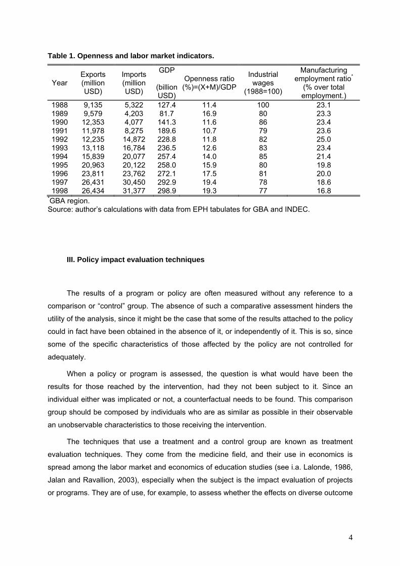
Table 1. Openness and labor market indicators.

Year Exports (million USD)

Imports (million USD)

GDP

(billion USD)

Openness ratio (%)=(X+M)/GDP

Industrial wages

(1988=100)

Manufacturing employment ratio*

(% over total employment.)

1988 9,135 5,322 127.4 11.4 100 23.1 1989 9,579 4,203 81.7 16.9 80 23.3 1990 12,353 4,077 141.3 11.6 86 23.4 1991 11,978 8,275 189.6 10.7 79 23.6 1992 12,235 14,872 228.8 11.8 82 25.0 1993 13,118 16,784 236.5 12.6 83 23.4 1994 15,839 20,077 257.4 14.0 85 21.4 1995 20,963 20,122 258.0 15.9 80 19.8 1996 23,811 23,762 272.1 17.5 81 20.0 1997 26,431 30,450 292.9 19.4 78 18.6 1998 26,434 31,377 298.9 19.3 77 16.8

*GBA region. Source: author’s calculations with data from EPH tabulates for GBA and INDEC.

III. Policy impact evaluation techniques

The results of a program or policy are often measured without any reference to a

comparison or “control” group. The absence of such a comparative assessment hinders the

utility of the analysis, since it might be the case that some of the results attached to the policy

could in fact have been obtained in the absence of it, or independently of it. This is so, since

some of the specific characteristics of those affected by the policy are not controlled for

adequately.

When a policy or program is assessed, the question is what would have been the

results for those reached by the intervention, had they not been subject to it. Since an

individual either was implicated or not, a counterfactual needs to be found. This comparison

group should be composed by individuals who are as similar as possible in their observable

an unobservable characteristics to those receiving the intervention.

The techniques that use a treatment and a control group are known as treatment

evaluation techniques. They come from the medicine field, and their use in economics is

spread among the labor market and economics of education studies (see i.a. Lalonde, 1986,

Jalan and Ravallion, 2003), especially when the subject is the impact evaluation of projects

or programs. They are of use, for example, to assess whether the effects on diverse outcome

4

variables (earnings, hours worked, test results) are explained by a specific policy, or if they

are the result of other contemporaneous changes.

These techniques may be divided in experimental and quasi-experimental2.

Experimental evaluations select randomly both the treatment group and the control group

before the policy or program is in effect. This random selection typically allows the four

mentioned conditions to occur. In economics, randomization is seldom possible or desirable,

since the selection of individuals who will participate in a given program might not be

independent of the expected results, thus selection bias appears. Also, some policies are

evaluated only after implementation, ought to the data requirements or the lack of means to

perform a thorough evaluation. Due to these difficulties, quasi-experimental evaluations are

more commonly found in the economics field. In these evaluations, treatment and

comparison groups are selected after the policy intervention is finished. The selection is

based on econometric techniques (matching or reflexive comparisons) that attempt to

account for the unobservable characteristics of the individuals, in a way that selection bias is

reduced to a minimum. Statistic techniques are used to correct for the differences in

characteristics among groups, so as to obtain results that measure as close as possible the

true effects of the policy change.

Despite the fact that the use of impact evaluation techniques in economics is subject to

some critics, most of which find objectionable that it does not rely on any parametric model;

the trade policy impact literature has begun to adapt the above-mentioned techniques to

address issues like the effects of trade opening on foreign direct investment, firms or industry

location and performance, and regional development (see Trefler, 2004; Girma et al., 2003).

Also, a few number of attempts were made to measure individual or household impacts of

trade liberalization using non-experimental evaluation (Balat and Porto, 2006; Toplalova,

2006, Hanson, 2006). The analysis in this paper is among this novel literature. Particularly, it

is the first in adapting the matching techniques to asses the impact of trade opening policies

on labor income levels and poverty.

IV. Discussion of the technique and estimation strategy

There are a variety of techniques to deal with non-experimental data, each of them

being suitable to evaluate a policy according to the framework of interest of the researcher

5

and the data available. They range from “before-after” analysis and a simple OLS regression,

to more advanced techniques which require the use of matching procedures, and whose

results exploit the difference-in-differences procedure. Matching techniques are frequently

used to evaluate reforms, and adjust to either longitudinal or cross-section data. Detailed

information on the individual in the sample or population is needed, for matching to avoid the

selection problem by constructing a comparison group of individuals with observable

characteristics as similar as possible to those of the affected by the policy reform (the

treated, in the terminology of impact evaluation).

In the case where longitudinal or repeated cross-section data is available, the

technique of difference-in-differences can provide a more robust estimate of the impact of the

reform under study, and significantly improves the evaluation if it is combined with matching

techniques (Heckman et al., 1997).

A full description of the techniques is beyond the scope of this study (for an overview

see Blundell and Costa Dias, 2000). However, a brief review of the concepts involved in this

study is in place.

Let y1it and y0

it be the outcome for an individual i in time period t (labor income,

expected wage and probability of unemployment will serve alternatively as response

variables in what follows), conditional on belonging or not to the treated tradable industries

sector, respectively. Denote by dit a dummy variable such as dit=1 if the individual i received

the treatment in period t, i.e. was related to the tradable manufactures directly affected by the

liberalization, and dit=0 if he was not in this group. Also, let Xit represent a vector of control

variables for each individual i in period t, namely attributes such as age or civil status, which

are unaffected by the policy under study.

For each individual, the policy impact is

Δ= y1it - y0

it. (1)

However, only one outcome variable is observed for each individual at any given

period t, which raises the missing-data problem. An estimate of the average impact of the

trade opening policy on the treated individuals is the average treatment on the treated (att),

the most widespread parameter in the microeconometric evaluation literature (Heckman et

al., 1997, 1998), defined as:

att = E (Δ | Xit, dit=1)

2 Of course, there are also non-experimental evaluation designs.

6

= E (y1it | Xit, dit=1) - E (y0

it | Xit , dit=1) (2),

where the last term in equation (2) is the average outcome the individuals in the affected

sectors would have shown, had they been in the unaffected group. This counterfactual is

estimated by the average outcomes of the individuals in the comparison group, E (y0it | Xit ,

dit=0). This is valid if some assumptions hold3. The main assumption is that of conditional

independence (CIA):

(y1it, y0

it) ⊥ dit | Xit (3).

CIA states that treatment status (dit) is random conditional on some set of attributes Xit ,

and independent of the potential outcomes (y1it, y0

it)4; which implies that given a set of

observable characteristics, the outcomes of a carefully defined group of individuals

unaffected by the policy can be used as counterfactuals of the outcome levels of the treated

had they not participated in the tradable industries. The matching procedure consists in

linking each treated case with a set of non-treated observations with the same values of Xit,

thus assuming that selection is only on observables (Heckman and Robb, 1985). To solve

the difficulty that arises when Xit is multidimensional, the results of Rosenbaum and Rubin

(1983) are useful, since it shows that if CIA holds conditional on Xit, it will also hold

conditional on a single index that captures all the information from those variables such as

P(Xit) =Pr (dit=1| Xit), the so-called propensity score. That is

(y1it, y0

it) ⊥ dit | P(Xit) (4).

Intuitively, if two groups have the same probability of being affected by the policy, they

will appear in the treatment and comparison group samples in equal proportions, therefore

they can be combined for purposes of comparison.

Notice also that to have empirical meaning, it is required that

0 < P(Xit) = Pr (dit=1| Xit) < 1 (5).

3 Following Rubin (1980), the outcome for each individual must be independent of other individuals’ treatment status. This is the stable unit-treatment value assumption that rules out inter- and/or intra-group spillover effects. The rest of necessary assumptions are treatment unconfoundedness and missing at random. See Heckman and Smith (1995) for a detailed discussion.

7

There must be observations from each group (treated and comparisons) for each

covariate in Xit. Otherwise, the analysis of treatment effects is limited only to the common

support region, which is the region where observations satisfy this condition.

According to (4) and (5), the att can be expressed as follows

att = E (Δ | dit=1, P P(Xit))

= EP [E (y1it | dit=1, P(Xit)) - E (y0

it | dit=0, P(Xit) | dit=1]

(6),

where EP is an expectation over the distribution of (P(Xit) | dit=1).

The method of double differences, or difference-in-differences, is an estimation method

to be used with both experimental and non-experimental design. They compare a treatment

and a comparison group (first difference) before and after the intervention (second

difference). A baseline survey is conducted for the outcome indicators for an untreated

comparison group as well as the treatment group before the intervention followed by another

survey after the intervention drawn from the same geographic clusters or strata in terms of

some variable.

The mean difference between the “after” and “before” values of the outcome indicators

for the treatment and comparison groups is calculated followed by the difference between

these two mean differences. The second difference (that is, the difference in differences) is

the estimate of the impact of the program or policy.

Heckman et al. (1997) and Heckman et al. (1998) introduced the difference-in-

differences matching estimator. This estimator has the potential to reduce sources of bias in

non-experimental settings. Intuitively, the benefits may arise from the fact that: i) relatively to

the propensity score matching estimator, the difference-in-differences matching adds the

control for non-observables, eliminating unobserved time-invariant differences in outcomes

across groups, while ii) relatively to the difference-in-differences estimator, its matching

version adds the comparability on observables that characterizes the propensity score

matching estimator.

With cross-sectional data, propensity score estimates of the average treatment effect

on the treated for each period –before and after – are computed and then the difference

between these two estimates yields the D-in-D matching estimate. Thus, (6) can be rewritten

4 In order to estimate the att parameter, it is sufficient to fulfill a condition less restrictive than CIA, which is conditional mean independence: E (y0

it | Xit, dit=1) = E (y0it | Xit , dit=0).

8

to exploit the availability of cross-sectional data for before (t=0) and after (t=1) the trade

opening, yielding the following expression of the difference-in-differences estimate:

attd-in-d = EP [E (y1i1 | di1=1, P(Xi1)) - E (y0

i1 | di1=0, P(Xi1) | di1=1]-

- EP [E (y1i0 | di0=1, P(Xi0)) - E (y0

i0 | di0=0, P(Xi0) | di0=1]

(7).

In practice, there is a wide variety of possibilities to conduct the matching procedure,

depending on the criterion for selection and weighting of the observations in the comparison

group. Each treated unit can be compared with a single match, with multiple non-treated

observations with or without replacement, or even with the entire comparison group, using

nearest neighbor matching, radius matching or kernel functions, respectively, and selecting

an appropriate weight function. The most common functions include the unity (identical)

weight(s) to the nearest observation(s) and zero to the rest, and kernel weights, which

penalize distant observations according to their propensity score. In most cases, increasing

the neighborhood or caliper to create the counterfactual will reduce the variance and amplify

the bias resulting from using more matches, some of which may be so distant that are of

inadequate comparability. Given the availability of data, a diversity of possible matching

schemes and weighting functions is explored in this study, including matching on Xit with the

Mahalanobis distance measure instead of the propensity score. The differences in the results

reflect the degree of overlap between treatment and comparison groups.

V. Data sources and variables

Data on outcome variables and individual characteristics are obtained from the

Argentinean Permanent Household Survey (EPH), waves May 1988 and May 1998,

corresponding to the Gran Buenos Aires region (GBA). GBA is economically the most

important urban region, representing nearly half of Argentina’s production and labor market.

The surveys are chosen to include a period before the trade opening (1988) which was not

affected by the turmoil of hyperinflation and crisis; and a point in time after the liberalization

(1998) which allows enough time for at least the medium-term effects of the policy to be in

place, and additionally is the last year in which the country’s economy performed

satisfactorily, before entering a recession that eventually led to a major socioeconomic crisis

in 2001.

9

The sample includes working age individuals (15 to 65 years old) that according to the

survey questionnaire worked either in the manufacturing sector (treatment group) or in areas

of the public sector that will be defined below (comparison group). Each individual in the

sample is classified by way of a dichotomous variable to belong to one of these two

categories.

The attributes for each observation in the sample are age (age), civil status (married),

position in the household (head), gender (gender), hours worked the week previous to the

survey (hour), years worked in the last job (histor), number of different occupations

(multiocup) and type of occupation i.e. entrepreneur, employed or independent worker

(emplo, indepw).

The outcome variables in this study are labor income (wages and hourly wages),

probability of unemployment, and expected wages. Monetary variables are measured in

constant pesos of 1999.

Labor earnings are the income variable chosen, with the aim of reducing the

measurement error that arises when multiple components of income are considered (i.e.

returns to capital, rents, public transfers and subsidies). Consequently, the analysis is on the

impacts of trade opening on labor income.

Hourly wages are included as an outcome variable to control for the possibility that

individual labor supply is affected differently across groups. Probability of unemployment and

expected wages (wages adjusted by the probability of employment) seek to reflect the

impacts of trade opening on unemployment. The individual’s unemployment probability is

calculated in this study with a standard logit model of unemployment on variables such as

age, gender, civil status, schooling and experience; for each one of the sample periods (May

1988 and May 1998).

In order to define the treatment and comparison groups, it is necessary to take into

account that the policy under consideration was not a set of measures targeted to specific

individuals. Rather, it is claimed that it has strong impacts in some sectors while leaving

other sectors unaffected. The association of individuals to each group mirrors, therefore, their

association to these segments of the economy.

In view of the stylized facts described in Section II, the election of the sectors included

in the treatment group is evident: they are the individuals who are linked, through the labor

market, to the tradable manufacturing industries, which were the industries directly affected

by the trade opening, given their low competitiveness relative to the rest of the world.

In opposition, and as is frequently the case in impact evaluation, the choice of a

counterfactual group is something of a challenge. This is true particularly if, as in the case

10

under study, a control group is not designated explicitly in the definition of the policy or

program. The comparison group in this study consists of the civil servants in every level of

the public administration (either state or sub-national), including teachers and doctors

working in the public sector.

This particular choice of comparable individuals requires additional justification for

those not familiar with the Argentinean economy and labor market. First, public employees

have a differential status relative to the private sector employees regarding the conditions of

entry, the possibilities of lay-offs, and the setting of their wages. Therefore, it is plausible to

assume they remained mostly unaffected by the trade policies that were in place in the

1990s. Evidence of relative less vulnerability of these workers to economic shocks is

presented in Corbacho et al. (2007). It is of importance for the analysis to have economic

and statistical validity, that the evolution of the variables for the individuals in the comparison

group remains as steady as possible in the period under analysis. Whilst it is an indisputable

fact that fiscal adjustments were required in Argentina in many of the years of the sample

period, they were mostly attained through a reduction in the state short-term contracts of

personal services, and seldom included reduction of permanent staff (Palomino, 2002)5. The

percentage of unemployed in this sector was 4% in 1988 and 6.1% in 1998, and the average

real wage increased a 13% in the sample period. It should be noticed also that not all the

public employees conform the abovementioned comparison group, since it was necessary to

remove from the sample those public workers linked to sectors such as services and state

enterprises (finance, communications, electricity, gas and water), for whom it was impossible

to assume away the existence of significant shocks during the 1990s, due to the massive

privatization and deregulation that affected them.

The second reason for the specific choice of individuals in the comparison group, is

that they share a similar set of characteristics with the individuals in the treatment group

(those in the tradable manufacturing sector), and accordingly a large region of common

support is obtained. Additionally, and regardless of these similarities, it is not likely that

intersectoral mobility takes place between both groups. On the one hand, individual labor

skills are very specific to each sector; and on the other hand there are institutional and

traditional barriers to entry in the public sector, preventing workers from the industrial sector

to move to government jobs.

5 Public employment abides to a specific regulation (currently Law number 25,164/1999). In addition, the union of public employees remains rather strong in the country: the last policy proposal of a reduction in nominal wages (of 13%) in March, 2001 was strongly rejected, and the minister of finance that proposed it was removed from functions one week after.

11

Finally, the inclusion as comparisons of alternative groups available in the EPH survey,

such as non-tradable sectors (i.e. commerce, construction, transport, housing), is not

adequate, because the general equilibrium effects of the trade opening affecting them are

likely to be important, and it will be impossible to rule out confounding effects in order to

establish causality. Barraud and Calfat (2008) shows evidence of significant impacts of tariff

reductions on wages in several non-tradable sectors. Moreover, the evolution of the

composition of employment in the sample period suggests an important shift of workers from

the manufacturing industry to several of these other sectors (Altimir and Beccaria, 1999).

VI. Results

Table 2 presents, for each of the periods under analysis, the estimates of the

propensity score of a dichotomous treatment variable that equals one if the individual is in

the tradable sector and zero if he is in the comparison group, regressed on the attributes

previously defined using a logit model. The independent variables to include in this

regression should be correlated to the outcome variables and to the participation in the

policy, but they should not be potentially changed by the policy itself. Thus, the choice of the

variables to include relies on economic theory, and prioritizes the use of time invariant

variables (age, gender, civil status).

The estimation results show that for both periods the conditional probability of working

in the tradable sector declines with the leading role in the household (head), the condition of

employee, the existence of more than one job and the work experience; while it increases for

married males who work more hours.

12

Table 2. Propensity score estimation

1998 1988 Variable Coef. Std. Err. z P>│z│ Coef. Std. Err. z P>│z│ age -0.0018 0.0053 -0.3400 0.7340 0.0004 0.0049 0.0800 0.9350head -0.1894 0.1302 -1.4500 0.1460 -0.0935 0.1218 -0.7700 0.4420married 0.0604 0.1137 0.5300 0.5950 0.0271 0.0994 0.2700 0.7850gender 1.1145 0.1210 9.2100 0.0000 0.8928 0.1087 8.2100 0.0000hour 0.0303 0.0032 9.5000 0.0000 0.0287 0.0029 9.8600 0.0000multiocup -1.7035 0.1607 -10.6000 0.0000 -1.7313 0.1369 -12.6500 0.0000emplo -0.3341 0.2473 -1.3500 0.1770 -0.8113 0.2497 -3.2500 0.0010indepw 0.5076 0.2958 1.7200 0.0860 -0.2232 0.2835 -0.7900 0.4310histor -0.0252 0.0073 -3.4600 0.0010 -0.0160 0.0060 -2.6700 0.0080constant -0.0200 0.3335 -0.0600 0.9520 1.0815 0.3206 3.3700 0.00101998: Number of obs=2022; LR chi2(9) =384.71; Prob > chi2 = 0.0000; Log likelihood = -1164.40; Pseudo R2 = 0.1418. 1988: Number of obs = 2553; LR chi2(9) = 427.24; Prob > chi2 =0.0000; Log likelihood = -1555.51; Pseudo R2 = 0.1207.

Along the lines of the recent literature on treatment evaluation, the reliability of the

propensity score matching procedure is carefully evaluated using balancing tests (see

Table3).

Table 3. Balancing tests

1998 1988 Variable Mean %reduct t-test Mean %reduct t-test Treated Control

%bias bias t p>│t│ Treated Control

%bias bias t p>│t│

age 36.974 37.147 -1.4 88.2 -0.27 0.785 35.791 35.661 1.0 84.4 0.26 0.794 head .52691 .52541 0.3 98.0 0.06 0.952 .53734 .53714 0.0 99.8 0.01 0.992 married .61952 .61535 0.9 83.9 0.17 0.864 .61586 .61593 0.0 99.8 -0.00 0.997

gender .73467 .74271 -1.7 97.2 -0.37 0.715 .71363 .72353 -

2.1 95.8 -0.56 0.575 hour 41.951 41.843 0.5 98.3 0.10 0.922 41.788 41.286 2.7 91.2 0.68 0.498 multiocup .92616 .93403 -1.6 96.0 -0.40 0.686 .98306 .97945 0.8 98.2 0.27 0.787

emplo .83104 .83985 -2.6 86.3 -0.47 0.635 .83834 .8605 -

6.5 56.7 -1.58 0.114 indepw .11514 .10121 4.8 68.3 0.90 0.370 .11008 .10351 2.2 67.8 0.54 0.587 histor 6.1765 6.0427 1.6 90.6 0.34 0.736 7.2871 7.1287 1.8 84.1 0.46 0.645 Results from the balancing tests after kernel matching with pstest (Leuven and Sianesi, 2003).

The standardized bias for each of the characteristics in Xit is examined following Smith

and Todd (2005). It is defined as the difference in means of each xit between the treatment

and the matched observations in the comparison set, scaled by the average variances of the

variable in these groups. Balancing or comparability will be higher the lower the standardized

13

difference. Additionally, a t-test of differences in means is performed after matching on the

propensity score for each variable entering the logit model.

In both periods, the results of the balancing tests show that the standardized bias

between individuals in the affected sector and the control sample are lower than 7% in the

common support region. Figure 1 shows the existence of a sizeable region of common

support in both years. Also, after performing (kernel) matching on the propensity score

depicted above, a considerable bias reduction is attained, suggesting that the approach

chosen in this study is appropriate since the comparison and treatment group of individuals

are indeed comparable.

According to Heckman et al. (1997), a program or policy is successfully evaluated if

there is a combination of data and methods that allows the following: i) the distribution of

unobservable characteristics is the same for treated individuals and comparison group; ii) the

distribution of observable characteristics is also the same for both groups; iii) the

measurement of outcomes and characteristics is conducted in the same way for the two

groups (same survey questionnaire); and iv) treatment and comparison groups come from

the same economic environment.

The assumptions of matching imply that condition i) holds. The success of the

balancing tests previously described ensures the verification of ii). Finally, as described in

Section V, the use of the same survey (EPH) for the same region (GBA) in both periods,

guarantee iii) and iv).

14

Figure 1. Common support 1a. 1998

0 .2 .4 .6 .8 1Propensity Score

Untreated Treated

1.b 1988

0 .2 .4 .6 .8 1Propensity Score

Untreated Treated

Number of individuals in each group, by propensity score. The region of common support is [.0515, .9608] in 1988 and [.0190, .9059] in 1998.

15

The impacts of trade opening on the outcomes of individuals in the manufacturing

tradable industries measured by the parameters in equations (6) and (7) are presented in

Table 4. They were estimated using the alternative computational methods currently

available.

Estimation I to IV correspond to the estimation of the average treatment effect on the

treated developed by Becker and Ichino (2002). Both I and II use nearest neighbor matching,

with the first using all observations and the second restricting the estimation to the common

support region, and using bootstrapped standard errors of the treatment effect. Estimation III

uses stratification matching based on the same stratification procedure used for estimating

the propensity score; by means of which in each block covariates are balanced (common

support is also imposed here). The att is computed using a weighted average of the block-

specific treatment effects, computed as the difference in average outcomes of treated and

comparison individuals within each stratum. In IV the att is calculated averaging over the

individual treatment effects, with the comparison to match to a treated unit obtained as a

Gaussian kernel-weighted average of control unit outcomes. Standard errors are

bootstrapped, which takes into account the uncertainty associated with the estimation of the

propensity score, since the region of common support changes with every bootstrap sample.

Rows V to VII show the results obtained with the implementations in Leuven and

Sianesi (2003). This procedure calculates approximate standard errors on the treatment

effects assuming independent observations, fixed weights, homoskedasticity of the outcome

variable within the treated and control groups, and that the variance of the outcome does not

depend on the propensity score. Row V uses the five nearest neighbors (or more in the case

of ties) with replacements. Row VII performs kernel matching as in IV, but in this case using

the Epanechnikov kernel. In VI, instead of the propensity score, full Mahalanobis-metric

matching is calculated on the same variables that entered the logit estimation (see Table 2)

including also the previously estimated propensity score.

Finally, following Abadie et al. (2004), the att parameter is estimated in rows VIII to X

using the three closest matches; without bias correction, with bias correction and

heteroskedasticty consistent standard errors, and imposing exact matches on the head and

emplo variables, respectively. The simple estimator will be biased in finite samples if the

matching is not exact, and will have a term corresponding to the discrepancies in covariates

between matched units and their matches (see Abadie et al., 2004). The selection of exact

matching in the head and emplo variables request employees that are head of their

households in the tradable sector, to be compared only to controls with exactly these same

two characteristics. This option is imposed in X, where the percentage of exact matches was

100%.

16

17

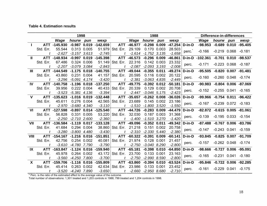
The different specifications of matching procedures, and the various choices about the

number and weighting of the comparison observations to use in the matching, did not result

in dispersion of the results, a feature that states the robustness of the findings and drive

away the reservations that frequently arise about these estimation procedures.

Remarkably, before and after the liberalization policy, labor market indicators of

individuals in the treatment group showed, in average, an inferior performance relative to the

values attained by the comparison units. What the difference in differences estimator shows

is that a significant worsening in the employment conditions of individuals in the tradable

group (relative to their matched counterparts) took place after the policy, a feature that may

therefore be regarded as a consequence of it. Depending on the estimation procedure, the

decrease in average real wages in the tradable industries is estimated in the interval 13%-

17%, and is even larger if measured by the hourly wage indicator, reaching relative

decreases estimated in 19% to 26% depending on the estimation procedure.

The deterioration of the labor situation for the treatment group after the economy was

open to international trade is also noticeable with the indicator of the probability of

unemployment, which was increased among 3% to 7% for the individuals linked to the

externally traded production. This led to an impact on their expected wages that reached

reductions of more than 18%.

18

Table 4. Estimation results 1998 1988 Difference-in-differences Wage hourw pun wexp Wage hourw pun wexp Wage hourw pun wexp

I ATT -145.930 -0.987 0.019 -142.659 ATT -46.977 -0.298 0.009 -47.254 D-in-D -98.953 -0.689 0.010 -95.405 Std. Err. 55.544 0.313 0.005 51.979 Std. Err. 29.109 0.170 0.003 28.503 t -2.627 -3.157 3.613 -2.745 t -1.614 -1.752 3.135 -1.658 perc.* -0.166 -0.219 0.068 -0.181

II ATT -148.934 -0.997 0.019 -145.398 ATT -46.573 -0.296 0.009 -46.861 D-in-D -102.361 -0.701 0.010 -98.537 Std. Err. 67.486 0.324 0.006 51.149 Std. Err. 22.316 0.142 0.003 23.332 t -2.207 -3.079 3.084 -2.843 t -2.087 -2.093 3.193 -2.008 perc. -0.171 -0.223 0.068 -0.187

III ATT -144.549 -1.175 0.018 -140.755 ATT -49.044 -0.355 0.011 -49.274 D-in-D -95.505 -0.820 0.007 -91.481 Std. Err. 43.860 0.231 0.004 41.157 Std. Err. 20.595 0.116 0.002 20.122 t -3.296 -5.091 4.174 -3.420 t -2.381 -3.063 4.835 -2.449 perc. -0.160 -0.260 0.048 -0.174

IV ATT -140.758 -1.196 0.018 -137.250 ATT -49.775 -0.392 0.012 -50.181 D-in-D -90.983 -0.804 0.006 -87.069 Std. Err. 39.956 0.222 0.004 40.433 Std. Err. 20.339 0.129 0.002 20.708 t -3.523 -5.381 4.136 -3.394 t -2.447 -3.046 5.175 -2.423 perc. -0.152 -0.255 0.041 -0.165

V ATT -135.623 -1.016 0.019 -132.448 ATT -35.657 -0.262 0.008 -36.026 D-in-D -99.966 -0.754 0.011 -96.422 Std. Err. 45.611 0.276 0.004 42.565 Std. Err. 23.689 0.145 0.002 23.186 t -2.970 -3.680 4.340 -3.110 t -1.510 -1.800 3.520 -1.550 perc. -0.167 -0.239 0.072 -0.183

VI ATT -127.598 -0.897 0.014 -125.540 ATT -44.726 -0.283 0.009 -44.479 D-in-D -82.872 -0.615 0.005 -81.061 Std. Err. 56.828 0.331 0.005 53.220 Std. Err. 32.030 0.187 0.003 31.368 t -2.250 -2.710 2.600 -2.360 t -1.400 -1.510 3.270 -1.420 perc. -0.139 -0.195 0.033 -0.154

VII ATT -136.584 -1.119 0.017 -133.128 ATT -49.096 -0.352 0.011 -49.342 D-in-D -87.488 -0.767 0.006 -83.786 Std. Err. 41.684 0.294 0.004 38.860 Std. Err. 21.218 0.151 0.002 20.758 t -3.280 -3.800 4.480 -3.430 t -2.310 -2.330 5.440 -2.380 perc. -0.147 -0.243 0.041 -0.159

VIII ATT -154.167 -1.216 0.016 -151.851 ATT -60.322 -0.391 0.009 -60.141 D-in-D -93.845 -0.825 0.007 -91.709 Std. Err. 42.756 0.254 0.002 40.081 Std. Err. 21.974 0.128 0.001 21.457 t -3.610 -4.780 7.790 -3.790 t -2.750 -3.040 8.290 -2.800 perc. -0.157 -0.262 0.048 -0.174

IX ATT -163.847 -1.124 0.016 -159.940 ATT -65.181 -0.398 0.010 -64.850 D-in-D -98.666 -0.727 0.006 -95.091 Std. Err. 45.978 0.264 0.002 43.172 Std. Err. 23.700 0.133 0.001 23.163 t -3.560 -4.250 7.800 -3.700 t -2.750 -2.990 8.590 -2.800 perc. -0.165 -0.231 0.041 -0.180

X ATT -159.706 -1.116 0.016 -155.809 ATT -63.860 -0.394 0.010 -63.524 D-in-D -95.846 -0.722 0.006 -92.285 Std. Err. 45.414 0.263 0.002 42.634 Std. Err. 23.986 0.133 0.001 23.452 t -3.520 -4.240 7.890 -3.650 t -2.660 -2.950 8.680 -2.710 perc. -0.161 -0.229 0.041 -0.175

* Perc. is the ratio of the estimated effect to the average value of the outcome. Total number of observations: 1,301 treated and 1,203 controls in 1988; 799 treated and 1,204 controls in 1998.

The treatment effects parameters are estimates of the average impact of the trade

policy on labor income of the individuals in the treatment group. However, they could mask

distributional changes if, for example, relative to the labor income of the comparison group,

the wages of individuals in the higher tail of the income distribution improved and the

earnings of those in the lowest percentiles worsened, or vice versa. This is important, since it

is significant to know the possible impact that the trade opening policy might have had on

poverty. By looking at the entire distribution of labor income, it is possible to asses the effects

of the trade opening on wage poverty, defined as the percentage of individuals whose wage

is not enough to attain a minimum consumption basket or poverty threshold, as defined by

the national statistics office, at 1999 prices6.

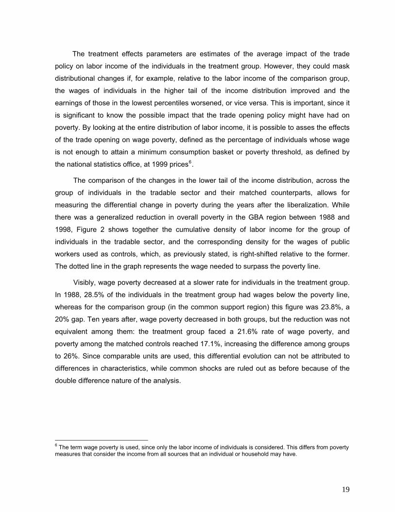
The comparison of the changes in the lower tail of the income distribution, across the

group of individuals in the tradable sector and their matched counterparts, allows for

measuring the differential change in poverty during the years after the liberalization. While

there was a generalized reduction in overall poverty in the GBA region between 1988 and

1998, Figure 2 shows together the cumulative density of labor income for the group of

individuals in the tradable sector, and the corresponding density for the wages of public

workers used as controls, which, as previously stated, is right-shifted relative to the former.

The dotted line in the graph represents the wage needed to surpass the poverty line.

Visibly, wage poverty decreased at a slower rate for individuals in the treatment group.

In 1988, 28.5% of the individuals in the treatment group had wages below the poverty line,

whereas for the comparison group (in the common support region) this figure was 23.8%, a

20% gap. Ten years after, wage poverty decreased in both groups, but the reduction was not

equivalent among them: the treatment group faced a 21.6% rate of wage poverty, and

poverty among the matched controls reached 17.1%, increasing the difference among groups

to 26%. Since comparable units are used, this differential evolution can not be attributed to

differences in characteristics, while common shocks are ruled out as before because of the

double difference nature of the analysis.

6 The term wage poverty is used, since only the labor income of individuals is considered. This differs from poverty measures that consider the income from all sources that an individual or household may have.

19

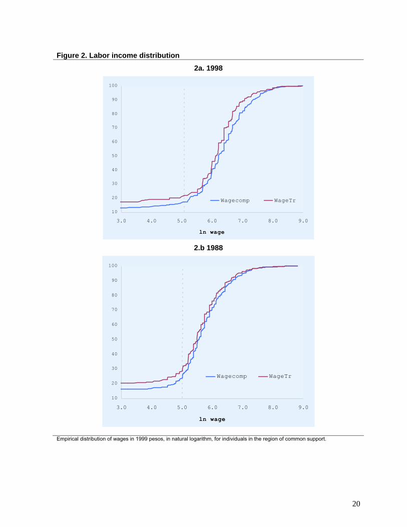
Figure 2. Labor income distribution

2a. 1998

10

20

30

40

50

60

70

80

90

100

3.0 4.0 5.0 6.0 7.0 8.0 9.0

ln wage

Wagecomp WageTr

2.b 1988

10

20

30

40

50

60

70

80

90

100

3.0 4.0 5.0 6.0 7.0 8.0 9.0

ln wage

Wagecomp WageTr

Empirical distribution of wages in 1999 pesos, in natural logarithm, for individuals in the region of common support.

20

VII. Conclusions

This study examined the changes in the labor income of individuals working in

industries that were directly affected by the Argentinean trade opening of the 1990s. The

manufacturing sector is the group where this policy had a larger impact, given their higher

exposure to external markets and their relative low competitiveness with respect to the rest of

the world.

There were many other policy changes in the period under analysis, which made

necessary to adopt an estimation strategy to control for this feature. The impact evaluation

technique of matching was chosen to estimate the impacts of the liberalization policy, making

use of a difference-in-differences approach, which takes advantage of the availability of

household surveys for a period before (1988) and a period after (1998) the policy.

To avoid confounding effects, the analysis centered on a particular region of the country

(GBA), and the comparison group was carefully chosen to provide an adequate

counterfactual of the without-the-policy condition. The control group consisted on public

employees, which are deemed to have been mostly isolated from the effects of the trade

policies.

It was estimated that real wages in the tradable industries decreased in the decade

after trade opening, and a reduction of 13% to 17% in the wages in this sector relative to the

wages in the comparison group may be directly attributed to this policy. Similarly, the

liberalization of trade produced an estimated relative increase of around 3% to 7% in the

probability of unemployment for the individuals linked to the tradable-goods production, and a

reduction in their relative expected wages that reached figures of more than 18%.

Poverty effects of the policy upon the individuals in the groups under analysis can also

be drawn. In a period in which poverty fell across all sectors, the changes in relative labor

income led to a slower reduction in the wage poverty rates in the tradable-producing group

compared to their matched counterparts.

The microeconomic consequences of a broad economic policy, such as a trade policy,

are often complex and difficult to measure and interpret. In this study the focus was explicitly

on the individuals related to the economic sectors more exposed to the global markets, and

therefore directly impacted by the policy. Suggestive evidence was found of a worsening in

21

their labor market outcomes in the medium-to-long term, in line with previous studies

(Barraud and Calfat, 2008).

22

References

Abadie, A., D. Drukker, J. Leber Herr, and G. W. Imbens (2004). Implementing

matching estimators for average treatment effects in Stata. Stata Journal 4: 290–311.

Altimir O., and L. Beccaria (1999). El mercado de trabajo bajo el nuevo régimen

económico en Argentina. CEPAL. Serie Reformas Económicas N° 28, Santiago, Chile.

Attanasio, O., Goldberg, P., and N. Pavcnik, (2004). Trade Reforms and Wage

Inequality in Colombia. Journal of Development Economics, 74: 331-366.

Balat, J., and G. Porto (2004). Globalization and Complementary Policies. Poverty

Impacts in Rural Zambia. In Harrison, A. ed., Globalization and Poverty. Chicago: University

of Chicago Press and the National Bureau of Economic Research.

Barraud, A. and G. Calfat (2008). Poverty effects from trade liberalization in Argentina.

Journal of Development Studies, Vol. 44, No. 3, 365–383, March 2008.

Becker, S. O., and A. Ichino, (2002). Estimation of average treatment effects based on

propensity scores. Stata Journal 2: 358–377.

Bertrand M., Duflo E., and S. Mullainathan. (2001). How much shoud we trust

differences-in-differences estimates. Cambridge: Massachusetts Institute of Technology,

Department of Economics, Working Paper Series Nº 01-34, 2001.

Blundell R., Costa Dias M., Meghir C., and J. Van Reenen (2001). Evaluating the

employment impact of a mandatory job search assistance program. The Institute for Fiscal

Studies Working Paper Nº 01/20, 2001.

Blundell R, Costa Dias M. (2000). Evaluation methods for non-experimetal data. Fiscal

Studies 21; 427-68.

Corbacho, A., Garcia-Escribano M. and G. Inchauste. (2007). Argentina:

Macroeconomic Crisis and Household Vulnerability. Review of Development Economics,

Blackwell Publishing, vol. 11(1), pages 92-106, 02.

Damill, M.; Frenkel, R. and Maurizio, R. (2002). Argentina: A decade of currency board.

An analysis of growth, employment and income distribution. Employment Paper Nº 42,

International Labour Organization, Geneva. Available at:

http://ilo.org/public/english/employment/strat/download/ep42.pdf

23

Feenstra, R. and G. Hanson. (1999). Productivity Measurement and the Impact of

Trade and Technology on Wages: Estimates for the U.S., 1972-1990. Quarterly Journal of

Economics, August, 114: 907-940.

Feenstra, R. and G. Hanson. (2003). Global Production and Inequality: A Survey of

Trade and Wages. In James Harrigan, ed., Handbook of International Trade, Basil Blackwell.

Freeman, Richard B. (1995) Are Your Wages Set in Beijing?. Journal of Economic

Perspectives, 9(1995):15-32.

Heckman J., Ichimura H., and P. Todd (1997). Matching as an econometric evaluation

estimator: evidence from evaluating a job training programme. Review of Economic Studies

1997; 64:605-54.

Heckman J., Ichimura H., and P. Todd (1998). Matching as an econometric evaluation

estimator. Review of Economic Studies 1998; 65:261-94.

Heckman J., Lalonde R., and J. Smith (1999). The econometrics of active labor market

programs. In: Ashenfelter O, Card D, ed. Handbook of labor economics. Vol. 3. Amsterdam:

North Holland, 1999; p. 1865-2097.

Heckman J., and R. Robb. (1985). Alternative methods for evaluating the impact of

interventions. An overview. Journal of Econometrics 1985; 30:239-67.

Jalan J, Ravallion M. (2003) Estimating the benefit incidence of an antipoverty program

by propensity score matching. Journal of Econometrics 2003;112:153-73.

Lalonde R. (1986) Evaluating the econometric evaluations of training programs with

experimental data. American Economic Review 1986;76:604-20.

Leuven, E., and B. Sianesi. (2003). "PSMATCH2: Stata module to perform full

Mahalanobis and propensity score matching, common support graphing, and covariate

imbalance testing," Statistical Software Components S432001, Boston College Department of

Economics, revised 28 Dec 2006. Available at:

http://ideas.repec.org/c/boc/bocode/s432001.html.

Robbins, D. (1996). Evidence on Trade and Wages in the Developing World. Technical

Paper N. 119.

Rosenbaum P., Rubin D. (1983) The central role of the propensity score in

observational studies for causal effects. Biometrika 1983; 70:41-55.

24

Smith, J., and P. Todd. (2005). Does matching overcome Lalonde’s critique of

nonexper-imental estimators? Journal of Econometrics 125: 305–353.

Topalova, P., (2006). Trade Liberalization, Poverty, and Inequality: Evidence from

Indian Districts. In Ann Harrison, ed., Globalization and Poverty. Chicago: University of

Chicago Press and the National Bureau of Economic Research.

25