an!agroecological!survey!of!urban! agriculture! sites!in...

1

An Agroecological Survey of Urban Agriculture Sites in the East Bay, California

A report to the Berkeley Food Institute

Miguel Altieri, Celine Pallud, Joshua Arnold, Courtney Glettner, Sarick Matzen, ESPM, UC-‐Berkeley

2

I. OBJECTIVES AND MOTIVATIONS

The purpose of this survey was to assess through an agroecological lens the main agronomic problems (soils, pests, weeds, diseases) limiting productivity affecting urban agriculture (UA) in East Bay Area. Our objective was two-‐fold: first, to determine cultural practices currently used by urban farmers and their effectiveness to overcome identified limiting factors; and second, to quantify actual yields reached in various urban farms subjected to varied soil and pest management practices under different spatial and temporal combinations of crops species and varieties. This information will provide a baseline that can be used to plan a series of on farm-‐research trials to explore urban agriculture best practices and management designs to overcome production constraints and optimize yields.

Farm managers were surveyed for soil and pest constraints and practices used, soil was sampled in various farms for nutrient and contaminant levels and two types of yield analysis were completed:

– Productivity quadrats: A 1m2 quadrat count was randomly placed on sampled beds in each farms (the number of quadrats was dependent on the size of the farm) in the early and late growing season. Number of crop species, plants/species, and vigor was assessed to estimate productivity for a given quadrat.

– Yield quadrats: Farmers were instructed to weigh all produce grown in designated 6m2 plots.

II. SURVEY DISTRIBUTION AND RESPONSE

This survey included 21 urban farms and gardens in Contra Costa and Alameda counties (Fig. 1.1). The survey captured three different categories of UA

Executive Summary This report summarizes a participatory community-‐based project carried out over the summer and fall of 2014 in 21 farms and gardens in the East Bay (Alameda and Contra Costa Counties) . We assessed urban farms to determine main agronomic problems limiting production, including soil quality and pest, weed and disease problems. Farms were assessed for productivity, and farmers were surveyed to determine main agronomic challenges and effectiveness of practices used to overcome constraints. Although results indicate that most farms have high soil fertility, and many farmers follow soil building practices and use techniques that emphasize high biodiversity, farmers face a number of issues related to insect and weed pressure, as well as problems linked to soil contamination and water use efficiency. Outreach should be targeted towards methods for increasing functional biodiversity, productivity with lower inputs and resiliency of farms.

3

including school gardens, community gardens and personal gardens that had been opened to the community. Participation in the surveys was varied due to limitations on farm managers’ availability.

• Sixteen sites completed the paper survey • Soil testing was conducted in 10 farms (as per cost constraints) • Fifteen farms had productivity measured via quadrat method • Six farmers reported total yields

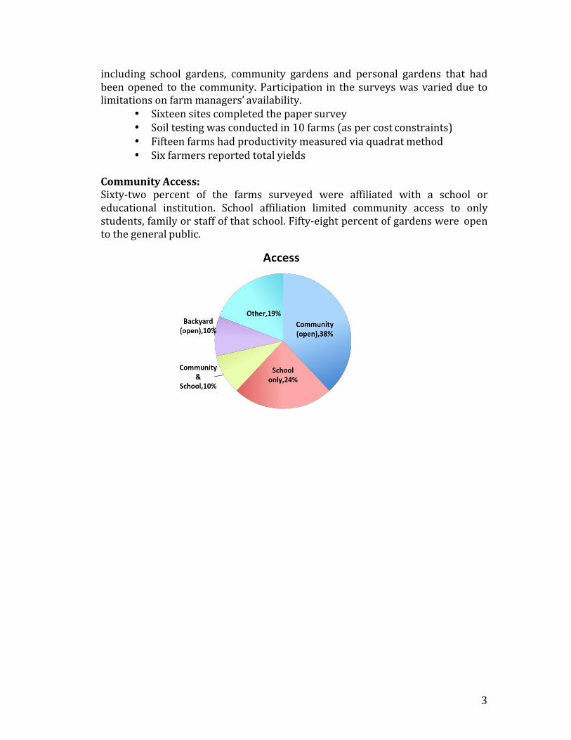
Community Access: Sixty-‐two percent of the farms surveyed were affiliated with a school or educational institution. School affiliation limited community access to only students, family or staff of that school. Fifty-‐eight percent of gardens were open to the general public.

4

Fig 1.1 Map of the 21 sites surveyed in the East Bay, Alameda and Contra Costa counties, CA

III. METHODS

Each farm manager was interviewed and completed a four page survey (27 questions). The survey gathered information on the organization, participating farmers, production challenges and farming practices used to overcome limiting factors. Our survey included 18 data categories:

– History of the land: What is the history of the space? What is the general story of the garden/farm?

– Mission of the farm/garden: What is the mission of the farm? What are the organizational goals?

– Legal land status: Does the farm have secure tenure in this space? – Labor: Who comprises the labor force? Is there paid farm labor or a

paid farm manager? – Experience of farmers: How experienced are the farmers and the

farm manager? – Access for community: Can the community access this land? Can

they rent plots or use the harvest from this space? – How does the farm acquire implements/tools, seeds and inputs?

5

– Crop plans: What crops are grown? Are they intercropping and does the farm have natural space or space that is not in production?

– Does the farm incorporate animals? – Pest, disease and weeds: What are the main pest problems and what

methods are they using to prevent or deal with them? – Soil Practices: How do they manage soil fertility? Are they recycling

nutrients on-‐farm? – Has the soil been tested for nutrients and contaminants? – Are they utilizing practices or infrastructure to conserve water? – How is the harvest distributed? – What is the size of the farm and the size (m2) of the production

space?

Soil Samples: In conjunction with UCANR, we sampled soil at ten farms. Each farm was sampled in three different areas and samples were tested for soil fertility and quality parameters and trace metal content, as described in Table 1.1. For each area, composite samples were taken in triplicate by combining four subsamples into one sample.

Fertility analysis was completed by UMASS Soil and Plant Tissue Testing Laboratory (Amherst, MA). Quality measurements were begun in the field and completed in the Pallud Lab. Trace metal analysis was completed by Curtis and Tompkins Laboratory (Berkeley, CA).

Table 1. Analyses completed on soil samples from different areas Area sampled Analysis Vegetable bed: An area currently in production, planted with tomatoes (or leafy greens, if no tomatoes were planted)

Fertility: pH, extractable macro and micronutrients, nitrate, percent organic matter, cation exchange capacity, extractable lead and aluminum, percent base saturation Quality: texture, bulk density, infiltration rate Trace metal content: arsenic, barium, cadmium, chromium, mercury, nickel, lead

High risk area: An area of concern that the farm manager would like to put into production

Trace metal content: arsenic, barium, cadmium, chromium, mercury, nickel, lead

Native soil: A pathway or open space in the farm, representing unamended soil conditions

Trace metal content: arsenic, barium, cadmium, chromium, mercury, nickel, lead

6

Productivity Quadrats: Quadrat sampling was used to estimate possible productivity yields for 19 farms in the study. The methodology used to estimate the average potential yields per square-‐meter are based on prior work by Altieri et al. and Colasanti and Hamm (2010). At two sampling intervals (May/June and August/September), data from 5 to 20, 1m2 quadrats was gathered depending on the size of the farm. The number of samples per farm was proportional to the overall size of each farm. Sampling locations were randomly selected throughout each farm. For each 1 m2

quadrat, the following data was collected: the number of species, number of plants per species, number of varieties per species, plant vigor, percent cover of weeds, weed community composition (broadleaf weeds, grass weeds, or mixed), the presence of any edible weed species, % of crop biomass affected by insect pests or diseases ( % crop damage) and % soil cover (presence of mulch).

Estimated yields on a per plant basis for each crop species were calculated based on John Jeavons (2012) estimates for yields potentially attained by an intermediate-‐good gardener using intensive, agroecological practices. If yield estimates were not available for a particular crop, additional sources were used (see appendix for crop yield estimates). Productivity estimates for each m2

sampled were calculated by multiplying the number of each species by its estimated yield. Estimated yields were reduced by 50 to 75% if the plant was in poor health or otherwise compromised, based on assessments of plant vigor or pest incidence.

Self-‐Reported Yield: Ten farms had 6m2 quadrats installed and were given scales and notebooks for recording purposes. Farmers were supposed to weigh the harvest from these areas. This technique did not have successful results, resulting in lower yield reporting. However, six of the participating farms weighed their harvest annually. We used this data and divided it by the total production area measured by our research teams to develop a per m2 result.

IV. RESULTS

Soil Results Summary: Nine out of ten sites had high soil fertility and exhibited good soil quality indicators. No samples contained elevated levels of total trace metals. Most gardeners surveyed followed agroecological practices to maintain soil fertility and quality. These finding were contrary to our expectations; we anticipated observing more farms with poor soil quality and some sites with trace metal contamination.

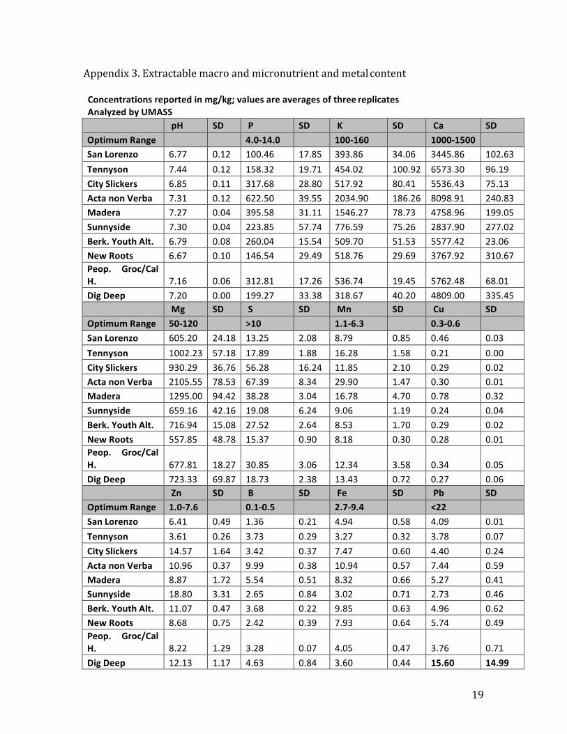
Fertility and Soil Quality: While certain macro-‐ and micro-‐nutrient levels were high across all sites (Appendix 3), representing typical conditions in East Bay soils, some trends emerged that allowed us to classify sites by percent organic matter, cation

7

exchange capacity, and bulk density (Appendix 4). Cation exchange capacity (CEC) is a measure of the soil’s ability to retain nutrients. Bulk density is the weight of soil per unit volume, an indication of soil components and compaction.

Percent organic matter and bulk density were inversely correlated (Figure 1.2.). Infiltration data had a high margin of error and is not reported here. Our fertility and quality results were bookended by Acta non Verba on the high end, with high organic matter, cation exchange capacity (CEC), nutrient contents, and low bulk density. On the low end, the poor soil quality (low organic matter, high bulk density) at Sunnyside could be detrimental to yields. Sites fell into two middle groups defined by moderate-‐high percent organic matter (City Slickers, Madera Elementary, and Berkeley Youth Alternatives), and moderate-‐low percent organic matter (San Lorenzo, Tennyson, New Roots, Dig Deep, Peoples’ Grocery).

We suspect that these groupings indicate different practices regarding compost amendment. Seventy-‐five percent of farms are composting on-‐site, with the remaining 25% citing labor restrictions for not composting. Farms also relied on municipal compost. While all sites added compost, the amount added is related to both cultural decisions and labor, and the effect of the compost is a function of amount added and quality of the compost. Some sites in the moderate-‐low grouping are school gardens that rely on student labor and serve an educational purpose that is equally important as food production (e.g., San Lorenzo). Future research would consider the degree to which community garden yields depend on compost amendment, with the goal of identifying lower and upper threshold levels of compost amending. Could some sites spend less energy applying compost, while achieving the same yields?

Figure 1.2 Soil organic matter and bulk density at various UA farms

All sites exhibited high soil levels of phosphorus, potassium, calcium, magnesium, and manganese. East Bay soils are generally high in calcium and magnesium. High phosphorus can be associated with watershed pollution, and

35

30

25

20

15

10

5

0

1.6 1.4 1.2 1 0.8 0.6 0.4 0.2 0

% OM

Bulk density, g/cm3

8

could be associated with high compost application rates. More research is needed to determine if the high phosphorus observed in these systems is lost via runoff and contributing to water pollution, or is utilized by plants to ensure high biomass production.

Soil texture analysis, a time-‐consuming process, is on-‐going. Results for 4 sites indicate loams (City Slickers, Berkeley Youth Alternatives, San Lorenzo) and silt loam (Acta non Verba). Loams are ideal agricultural soils. It will be interesting to see if any soils are high in clay, a hallmark of East Bay soils, which can lead to poor drainage and poor structure.

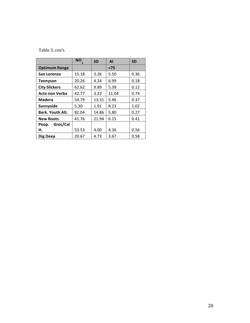
Trace Metal Contamination: Thorough analysis of the trace metal concentration data is challenging because there are no federal guidelines for trace metal concentrations in agricultural soils (US EPA, 2011). However, no samples exceed the levels for total arsenic, cadmium, lead, or zinc recommended by the EPA Region 5 Technical Remediation for Brownfields program, which advises community groups seeking to redevelop brownfields into urban agricultural sites (Leven, 2014) (Appendix e 5). One sample out of 30, one of the three replicate samples taken from Dig Deep Farm, had elevated extractable lead. The wide range of concentrations measured in the Dig Deep Farm samples indicates hotspots of high lead, but not elevated levels overall. Compost amending is recommended for tying up lead and thus making it less bioaccessible, and also diluting existing lead in soil. Dig Deep was in the group of sites with moderate-‐low organic matters, so we would recommend that they add more compost to both stabilize contaminants and increase fertility overall.

Water: The obvious need for irrigation is often complicated by urban water prices and access. All but two respondents related that if the farm itself was responsible for irrigation costs they would not be able to operate the farm. Fifty-‐two percent of surveyed farms had an organization or partner that covered the costs of irrigation. Many farms are on city property and have MOU’s with the related city that provides that the city itself pays for irrigation needs. Only 10% of the farms (2) had wells that were used for irrigation and both related that they were worried about the quality of the water and also the possibility of the well running dry. One respondent was able to acquire agricultural rates from East Bay Municipal Utilities District (EBMUD).

On-‐farm animals: Less than half of the farms surveyed had on-‐farm animals (chicken, goats, ducks, worms or bees). Raising chickens was the most popular (42%) animal activity; chicken ate ,uch of the crop residues and also provided manure. Keeping animals showed a positive correlation with on-‐farm soil building. Ducks and sheep were represented at 5% with worms and bees at 18% and 29% respectively.

9

Insect Pests: Most respondents felt that pest problems were not as much of a pressing issue as we expected. Many farmers were following best practices to promote beneficial insects for biological control such as having habitat strips, intercropping or planting flowers and facilitating a more heterogeneous crop plan. Despite these measures, some pests were prevalent such as cabbage aphids often tended by argentine ants, snails, slugs and leaf miners which under certain conditions could inflict high levels of damage (Figure 1.3). Common practices to control aphids are hand-‐washing the plants or spraying aphids off with a hose. Symphylans, an often-‐unknown pest related to millipedes that eats roots, was often mentioned. Interestingly, the Peoples Grocery Hotel California location believes that planting fava beans seem to have helped reduce symphylan levels in their garden.

Fig 1.3 Prevalent pests observed and reported in UA surveys

The majority of respondents believe that measures they are using to prevent pests are effective (Figure 1.4). Using homemade sprays or organic approved pesticide sprays was common but most respondents said these techniques were not very effective. Generally, most farms recognized that soil health, on-‐farm biodiversity and plant vigor helped repel pests most effectively. Effectiveness of various pest control practices are anecdotal and warrant further research.

Pests 80% 70% 60% 50% 40% 30% 20% 10% 0%

% of farms reported

10

Fig 1.4 Most common methods of pest control

Weeds: Many farmers struggled with weeds. However, the majority of farmers mentioned that methods used to control or prevent are “effective” to “generally effective”. Some farmers take advantage of “weed” cover after plants get past their period of critical competition, but most allow presence and growth of aggressive weeds (amaranth, grasses) to levels that reduce crop yields. Joseph, the farm manager at Union Plaza, said weeds like wild radish are “okay” because they provide ground cover. A few of the gardens (SOGA, Tennyson and Union Plaza) suggested that using a hoe to weed can be counter-‐productive because you create a better habitat for weed growth.

Weed Community Data: Percent cover of weeds in each quadrat also varied by farm. Some farms had very low weed densities (or no weeds), but in others, weeds reached high presence. However, average weed cover in quadrats sampled was 7.13 %/ m2 (Table 2) Over half of the quadrats sampled were in raised beds, our observations suggest that raised beds typically exhibited lower weed densities. Broadleaf weeds were prevalent in the quadrats, while most weed communities consisted of broadleaf weeds only, many quadrats exhibited combinations of broadleaf weeds mixed with grasses ( Figure 1.6 and 1.7). Dominance of grass weeds signaled low yields in many plots. Many of the weed species identified in this study were edible such as purslane, lambsquarters, malva , and amaranth. ( Figure 1.5).

Methods of Pest Control 45% 40% 35% 30% 25% 20% 15% 10% 5% 0%

% Of farms reported

11

Fig 1.5 Edible weeds present in East Bay urban farms

Table 2. Weed % cover in raised beds and plots with mulch

*Not all mulch cover was adequate to be effective; most was sparse (Fig 4.4)

Edible Weeds Present in East Bay Urban Farms

45 40 35 30 25 20 15 10 5 0

% Of farms responded

Overall Weed Data Summary

Percent weed cover/ m2

Percent of quadrats sampled in raised beds

Percent of quadrats sampled with mulch*

Mean 7.13 53.26 30.15 Standard deviation 8.08 -‐-‐-‐-‐-‐-‐ -‐-‐-‐-‐-‐-‐

12

Fig 1.6 Weed community composition

Fig 1.7 Weed species

Weed Community Compostion

Average percent of quadrats sampled with only broadleaf weeds

40.09 % No weeds

31.22 % Broadleaf weeds only

Average percent of quadrats sampled with only grass weeds

20.94 % Mixed weed community

Average percent of quadrats sampled with a mixed weed

7.76 % community

Grass weeds No weeds present only

Weed Species 50% 45% 40% 35% 30% 25% 20% 15% 10% 5% 0%

% Of repondents

13

Weed Control 70%

60%

50%

40%

30%

20%

10%

0%

Fig 1.8. Weed control cultural practices

Weed control: There was a wide range of weed control methods used by surveyed farmers (Figure 1.8). Hand weeding was effective only if done timely in relation to the weed critical period of competition. Thirty percent of the quadrats sampled had some form of mulch. However, in many of these cases, the mulch cover was very light and was not effective in blocking weeds, but in plots with a thick mulch weed suppression was high.

Productivity: Estimated productivity results varied among farms (Appendix 1), most likely due, in part, to the diversity of goals, labor support, and organizational characteristics of each farm, as recognized by the interview results. Average estimated seasonal yield ranged from 3.43 kg/m2 to 17.16 kg/m2 , with a mean productivity of 7.09 kg/m2 for all farms included in the study (Table 3). This estimate is less than the targeted 10 kg/m2 of productivity (established by our team based on production levels reached by intermediate Cuban urban farms) and demonstrates the potential for increased yields in Bay Area urban agriculture with additional research, outreach, and institutional support. Low yields seemed associated with poor choice of crops, bad management and low levels of crop diversity. A large number of heavy, high producing crops (tomato, squash, and strawberry) resulted in high estimated productivity and are hypothesized to be a large factor in the variation seen in the data. Additionally, weight is not the only way of measuring productivity, in farms using intercropping systems a more appropriate method is the use of the Land Equivalent Ratio.

% Of respondents

14

Table 3. Overall farm productivity summary Overall Productivity

Farm level species diversity

Garden-‐bed level species diversity

Garden-‐bed level genetic diversity

Productivity

Total # crops grown (normalized by size)

Average # spp/m2

Average # varieties/spp/m2

Average estimated yield lbs/ft2

Average estimated yield kg/m2

Mean 1.63 2.84 1.37 1.45 7.09 Standard deviation

0.54

1.08

0.66

0.67

3.25

V. RATINGS

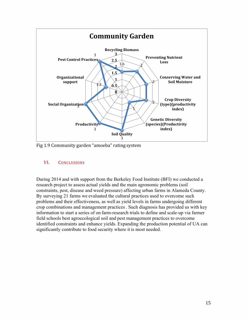
Each farm was “graded” using a metric created for this survey (see Appendix 2) using ten indicator criteria . Each indicator was given a rating (based on a score of 0-‐3) or based on the yield scale previously discussed. Ratings were put into an “amoeba” type information graphic ( Figure 1.9) and included in a final agroecological report to be issued to each farm to help farmers identify their weak pints ( indicators with low scores), adopt social and management practices to improve score of low indicators and thus improve overall performance of each farm. We will use this methodology in future farmer-‐to-‐ farmer trainings.

15

Fig 1.9 Community garden “amoeba” rating system

VI. CONCLUSIONS During 2014 and with support from the Berkeley Food Institute (BFI) we conducted a research project to assess actual yields and the main agronomic problems (soil constraints, pest, disease and weed pressure) affecting urban farms in Alameda County. By surveying 21 farms we evaluated the cultural practices used to overcome such problems and their effectiveness, as well as yield levels in farms undergoing different crop combinations and management practices . Such diagnosis has provided us with key information to start a series of on farm-research trials to define and scale-up via farmer field schools best agroecological soil and pest management practices to overcome identified constraints and enhance yields. Expanding the production potential of UA can significantly contribute to food security where it is most needed.

Community Garden

3 Pest Control Practices

Recycling Biomass 3

2.5 1.6 2

Preventing Nutrient Loss

Organizational support 1.3

2 1.5 1

0.5 0

Conserving Water and 2 Soil Moisture

Social Organization 2 3 1

Crop Diversity (type)(productivity

index)

Productivity 3

Genetic Diversity (species)(Productivity

index) Soil Quality

3

16

VII. REFERENCES Leven, B. 2014. What We Tell Cities and Community Gardeners:

Approaches to Safe, Productive Gardens, July 2, 2014, Soils in the City Conference. Chicago, Illinois

US EPA. 2011. Brownfields and urban agriculture: Interim guidelines for safe

gardening practices. Available at www.epa.gov/brownfields

17

Appendix 1. Average species diversity and yields, by farm Farm #

Total area of beds under production (m2)*

Average (by farm) Notes

Farm level species diversity

Garden-‐ bed level species diversity

Garden-‐ bed level genetic diversity

Productivity

Total # crops grown (normalized by size)

Average # spp/m2

Average # varieties /spp/m2

Average estimated yield lbs/ft2

Average estimated yield kg/m2

1 101.7 1.13 1.50 1.25 3.52 17.16 Lots of strawberry plants 2

138.6

1.83

2.93

1.05

1.15

5.60

Total area only includes garden beds in production, not permaculture hillside

3 299.7 2.33 2.21 2.76 1.09 5.30 4

440.1

0.70

1.68

1.15

2.42

11.80

Lots of strawberry, squash, tomato plants

5 56.0 1.50 2.88 1.05 1.10 5.37

6 136.3 1.41 2.24 1.00 1.51 7.38 Lots of strawberry plants 7

36.8

1.58

3.17

1.00

2.03

9.92

Lots of strawberry, tomato plants

8

96.5

1.95

2.88

1.13

1.22

5.94

Due to lead and summer, sample #2 estimated yeild was very low

9 10.6 2.40 5.10 1.16 1.63 7.97 Lots of tomato plants 10

8016.0

1.61

3.12

1.01

1.19

5.78

Total UC village (from ArcMap) 8,438 m2

assuming ~5% for paths = 8016 m2

11 31.3 2.50 5.30 1.13 1.31 6.40

12 123.1 1.67 2.43 1.42 0.91 4.43

13 24.1 1.80 4.30 1.02 1.64 8.00 Lots of tomato plants 14

178.8

1.30

1.93

2.05

0.99

4.84

Lots of strawberry, squash plants in sample #2

15 495.3 0.98 2.27 1.13 1.18 5.77 16

1.03

2.44

1.21

1.12

5.47

Lots of tomato, squash plants

17 2.60 3.66 3.40 2.00 9.75

18 179.4 1.08 2.00 1.08 0.89 4.34

19 565.5 1.57 2.00 1.00 0.70 3.43

18

Appendix 2. Survey grading matrix

19

Appendix 3. Extractable macro and micronutrient and metal content Concentrations reported in mg/kg; values are averages of three replicates Analyzed by UMASS

pH SD P SD K SD Ca SD Optimum Range 4.0-‐14.0 100-‐160 1000-‐1500 San Lorenzo 6.77 0.12 100.46 17.85 393.86 34.06 3445.86 102.63 Tennyson 7.44 0.12 158.32 19.71 454.02 100.92 6573.30 96.19 City Slickers 6.85 0.11 317.68 28.80 517.92 80.41 5536.43 75.13 Acta non Verba 7.31 0.12 622.50 39.55 2034.90 186.26 8098.91 240.83 Madera 7.27 0.04 395.58 31.11 1546.27 78.73 4758.96 199.05 Sunnyside 7.30 0.04 223.85 57.74 776.59 75.26 2837.90 277.02 Berk. Youth Alt. 6.79 0.08 260.04 15.54 509.70 51.53 5577.42 23.06 New Roots 6.67 0.10 146.54 29.49 518.76 29.69 3767.92 310.67 Peop. Groc/Cal H.

7.16

0.06

312.81

17.26

536.74

19.45

5762.48

68.01

Dig Deep 7.20 0.00 199.27 33.38 318.67 40.20 4809.00 335.45 Mg SD S SD Mn SD Cu SD Optimum Range 50-‐120 >10 1.1-‐6.3 0.3-‐0.6 San Lorenzo 605.20 24.18 13.25 2.08 8.79 0.85 0.46 0.03 Tennyson 1002.23 57.18 17.89 1.88 16.28 1.58 0.21 0.00 City Slickers 930.29 36.76 56.28 16.24 11.85 2.10 0.29 0.02 Acta non Verba 2105.55 78.53 67.39 8.34 29.90 1.47 0.30 0.01 Madera 1295.00 94.42 38.28 3.04 16.78 4.70 0.78 0.32 Sunnyside 659.16 42.16 19.08 6.24 9.06 1.19 0.24 0.04 Berk. Youth Alt. 716.94 15.08 27.52 2.64 8.53 1.70 0.29 0.02 New Roots 557.85 48.78 15.37 0.90 8.18 0.30 0.28 0.01 Peop. Groc/Cal H.

677.81

18.27

30.85

3.06

12.34

3.58

0.34

0.05

Dig Deep 723.33 69.87 18.73 2.38 13.43 0.72 0.27 0.06 Zn SD B SD Fe SD Pb SD Optimum Range 1.0-‐7.6 0.1-‐0.5 2.7-‐9.4 <22 San Lorenzo 6.41 0.49 1.36 0.21 4.94 0.58 4.09 0.01 Tennyson 3.61 0.26 3.73 0.29 3.27 0.32 3.78 0.07 City Slickers 14.57 1.64 3.42 0.37 7.47 0.60 4.40 0.24 Acta non Verba 10.96 0.37 9.99 0.38 10.94 0.57 7.44 0.59 Madera 8.87 1.72 5.54 0.51 8.32 0.66 5.27 0.41 Sunnyside 18.80 3.31 2.65 0.84 3.02 0.71 2.73 0.46 Berk. Youth Alt. 11.07 0.47 3.68 0.22 9.85 0.63 4.96 0.62 New Roots 8.68 0.75 2.42 0.39 7.93 0.64 5.74 0.49 Peop. Groc/Cal H.

8.22

1.29

3.28

0.07

4.05

0.47

3.76

0.71

Dig Deep 12.13 1.17 4.63 0.84 3.60 0.44 15.60 14.99

20

Table 3, con’t.

NO -‐

3 SD Al SD Optimum Range <75 San Lorenzo 15.18 3.26 5.50 0.36 Tennyson 20.26 4.24 6.99 0.18 City Slickers 62.62 9.89 5.39 0.12 Acta non Verba 42.77 3.22 11.04 0.74 Madera 54.79 13.31 5.46 0.37 Sunnyside 5.30 1.91 8.23 1.02 Berk. Youth Alt. 82.04 14.86 5.80 0.27 New Roots 41.76 21.94 6.15 0.41 Peop. Groc/Cal H.

53.53

4.00

4.36

0.56

Dig Deep 20.67 4.73 3.67 0.58

21

Appendix 4. Exchangeable acidity, CEC, percent base saturation, and organic matter Ex.

Acidity SD CEC SD Ca BS, % SD Mg BS, % SD

Optimum Range 50-‐80 10.0-‐ 30.0

San Lorenzo 0.96 0.13 24.16 0.70 71.31 0.36 20.53 0.25 Tennyson 0.00 0.00 42.24 1.03 77.82 1.24 19.44 0.70 City Slickers 0.26 0.23 36.89 0.67 75.05 0.90 20.67 0.45 Acta non Verba 0.00 0.00 62.96 2.22 64.33 0.64 27.41 0.11 Madera 0.00 0.00 38.36 1.51 62.04 1.69 27.65 1.32 Sunnyside 0.00 0.00 21.58 1.86 65.72 1.13 25.08 1.00 Berk. Youth Alt. 1.26 0.07 36.33 0.26 76.76 0.51 16.17 0.23 New Roots 2.50 1.00 27.24 0.99 69.08 3.27 16.76 0.90 Peop. Groc/Cal Hotel

0.00

0.00

35.75

0.55

80.53

0.50

15.54

0.50

Dig Deep 0.00 0.00 30.80 2.26 78.00 1.00 19.33 0.58 K BS, % SD Scp

Dens, SD OM, % SD

Optimum Range 2.0-‐7.0 g/cc San Lorenzo 4.17 0.26 0.99 0.06 9.05 1.99 Tennyson 2.74 0.54 0.98 0.07 8.84 1.26 City Slickers 3.58 0.50 0.78 0.04 18.09 0.44 Acta non Verba 8.26 0.53 0.60 0.01 31.24 1.77 Madera 10.31 0.44 0.86 0.00 17.36 2.76 Sunnyside 9.20 0.25 1.05 0.04 4.73 0.70 Berk. Youth Alt. 3.59 0.36 0.77 0.05 17.99 0.22 New Roots 4.87 0.17 0.92 0.03 11.72 0.59 Peop. Groc/Cal Hotel

3.93

0.13

0.93

0.08

9.85

0.51

Dig Deep 2.67 0.58 0.90 0.01 12.50 1.67

22

Appendix 5. Trace metal analysis for selected sites Vegetable bed Area of concern Path/native soil

Site Name Avg mg/kg

SD

Avg mg/kg

SD

Avg mg/kg

SD

San Lorenzo High School

Arsenic 13.3 1.2 3.9 0.3 13.7 0.9 Barium 113.3 4.7 203.3 18.9 136.7 4.7 Cadmium 0.5 0.0 0.5 0.1 0.5 0.0 Chromium 29.0 2.2 47.0 12.8 30.0 0.8 Mercury 0.1 0.0 0.2 0.0 0.1 0.0 Nickel 27.3 0.9 35.3 1.2 29.0 0.8 Lead 44.0 0.8 78.0 22.9 75.3 31.6

Tennyson High School


Acta Non Verba


Dig Deep Firehouse


People's Grocery


IRC New Roots


City Slickers Union Plaza


23

Berkeley Alternative Youth Production Garden


Metals analysis completed by UC ANR in collaboration with Altieri and Pallud BFI Urban Agricultural Survey Samples analyzed by Curtis and Tompkins Laboratory, Berkeley, CA Due to regulatory constraints, UC ANR was not able to fund metals testing for some sites surveyed by Altieri and Pallud. Average and standard deviation of three composite samples composed of 4 subsamples each

an!agroecological!survey!of!urban! agriculture! sites!in...

Documents