ana paula palacios june 28, 2012 - core.ac.uk · aplicable a una gran variedad de microorganismos y...
TRANSCRIPT

Models and inference for population dynamics
Ana Paula Palacios
June 28, 2012


A mis padres


“Essentially, all models are wrong, but some are useful.”
George E. P. Box


Agradecimientos
En primer lugar quisiera agradecer a mis directores por su incondicional apoyoy por todo lo que me han ensenado. Mike, gracias por tu increıble lucidezy conocimiento, especialmente en las tardes que compartimos en la biblioteca.Juanmi, gracias por ayudarme en mi lucha personal contra los codigos, por tuaporte biologico y revolucionario, y fundamentalmente por tu paciencia y por tucomprension.
En segundo lugar, pero con la misma importancia, quisiera agradecer a mifamilia, a mis padres y a mi hermana. Quiero darles las gracias, profundamente,por dejarme vivir mi propio camino, por apoyarme en esta y en cada cosa que mepropongo. Por sufrir (tanto como yo) la distancia, pero a pesar de eso brindarmetodo su amor de manera incondicional.
Tambien quisiera agradecer a Peter, quien fue muy importante en una etapadurante este perıodo de tesis. Gracias por ser fundamentalmente mi apoyo emo-cional en estas tierras lejanas, gracias por nuestras charlas academicas a cualquierhora del dıa, por tus comentarios y por tu infinita paciencia cuando me explicabasalgo.
No quiero olvidarme de nadie, y hare mi mejor intento. Dolo, Lu, Santi yAle, gracias a ustedes estoy hoy aquı. Ana, Caro y Jona, ustedes fueron comomis hermanos en Madrid, gracias por su amor fraternal. A la banda, Juancho,Diego, Gabi, Huro, gracias por hacerme sentir mas cerca de Cordoba. Eli, Ramony especialmente Irene, gracias por acompanarme en mi estancia en Colmenarejo.Carles, Bernardo y Fabrizio, gracias por su buena predisposicion a responder mispreguntas y por sus valiosos comentarios. Emiliano, gracias a tu generosidadpudimos enriquecer esta tesis con las aplicaciones a datos reales de bacterias.Gracias a todos mis companeros y amigos, que de una manera u otra me hanayudado a cumplir mi objetivo: Audra, Adolfo, Leo, Carlo, Gabriel, Pato, Sofi, yAndrea. A mis amigos de Cordoba, Ivan, Malu, Sole, Lu, Caro y Guada, graciaspor su amistad a pesar de la distancia. Y como olvidarme de Mari y Visi, de susmimos y de esas ricas meriendas...
Gracias a todos ustedes, esto fue posible.
i

ii

Contents
Resumen xi
Introduction and Summary xiii
1 Single populations 1
1.1 Introduction . . . . . . . . . . . . . . . . . . . . . . . . . . . . . . 1
1.2 Population models . . . . . . . . . . . . . . . . . . . . . . . . . . 2
1.2.1 The Malthusian growth model . . . . . . . . . . . . . . . . 2
1.2.2 The logistic growth model . . . . . . . . . . . . . . . . . . 4
1.2.3 Delay models . . . . . . . . . . . . . . . . . . . . . . . . . 6
1.2.4 Models for interacting populations . . . . . . . . . . . . . 7
1.2.5 Stochastic models . . . . . . . . . . . . . . . . . . . . . . . 10
1.3 Bacterial growth models . . . . . . . . . . . . . . . . . . . . . . . 13
1.3.1 Gompertz model . . . . . . . . . . . . . . . . . . . . . . . 14
1.3.2 Baranyi model . . . . . . . . . . . . . . . . . . . . . . . . . 16
1.3.3 Three phase linear model . . . . . . . . . . . . . . . . . . . 18
1.3.4 Secondary models . . . . . . . . . . . . . . . . . . . . . . . 19
1.4 Model fitting . . . . . . . . . . . . . . . . . . . . . . . . . . . . . 20
1.4.1 Nonlinear Least Squares . . . . . . . . . . . . . . . . . . . 20
1.4.2 Bayesian estimation . . . . . . . . . . . . . . . . . . . . . . 22
1.5 Growth curve modeling using WinBUGS . . . . . . . . . . . . . . . 24
1.5.1 Model specification . . . . . . . . . . . . . . . . . . . . . . 24
1.5.2 Data analysis . . . . . . . . . . . . . . . . . . . . . . . . . 29
iii

iv CONTENTS
1.5.3 Model comparison . . . . . . . . . . . . . . . . . . . . . . 29
1.6 Application: Listeria monocytongenes . . . . . . . . . . . . . . . . 30
1.6.1 Bayesian inference . . . . . . . . . . . . . . . . . . . . . . 35
1.7 Conclusions . . . . . . . . . . . . . . . . . . . . . . . . . . . . . . 38
2 Hierarchical models 41
2.1 Introduction . . . . . . . . . . . . . . . . . . . . . . . . . . . . . . 42
2.1.1 Bayesian Hierarchical Modeling . . . . . . . . . . . . . . . 44
2.2 A hierarchical Gompertz model for bacterial growth . . . . . . . . 45
2.3 Bayesian inference . . . . . . . . . . . . . . . . . . . . . . . . . . 48
2.4 Application: Listeria monocytogenes . . . . . . . . . . . . . . . . 52
2.5 Conclusions . . . . . . . . . . . . . . . . . . . . . . . . . . . . . . 62
3 Neural networks models 63
3.1 Introduction . . . . . . . . . . . . . . . . . . . . . . . . . . . . . . 63
3.2 Secondary models . . . . . . . . . . . . . . . . . . . . . . . . . . . 64
3.2.1 The square-root model . . . . . . . . . . . . . . . . . . . . 65
3.2.2 Cardinal parameter models . . . . . . . . . . . . . . . . . 66
3.2.3 Polynomial models . . . . . . . . . . . . . . . . . . . . . . 67
3.2.4 Artificial neural network models . . . . . . . . . . . . . . . 68
3.3 Neural network based growth curve models . . . . . . . . . . . . . 68
3.3.1 Feed forward neural networks . . . . . . . . . . . . . . . . 69
3.3.2 A neural network based Gompertz model . . . . . . . . . . 71
3.3.3 A hierarchical neural network model . . . . . . . . . . . . 72
3.3.4 Error modeling . . . . . . . . . . . . . . . . . . . . . . . . 73
3.4 Bayesian inference for the neural network models . . . . . . . . . 74
3.4.1 Model selection . . . . . . . . . . . . . . . . . . . . . . . . 77
3.5 Application: Listeria monocytogenes . . . . . . . . . . . . . . . . 78
3.6 Conclusions . . . . . . . . . . . . . . . . . . . . . . . . . . . . . . 83
4 Stochastic models 85

CONTENTS v
4.1 Introduction . . . . . . . . . . . . . . . . . . . . . . . . . . . . . . 85
4.2 The model . . . . . . . . . . . . . . . . . . . . . . . . . . . . . . . 87
4.3 The mean function of the growth process . . . . . . . . . . . . . . 93
4.3.1 Transient state . . . . . . . . . . . . . . . . . . . . . . . . 94
4.3.2 Stationary state . . . . . . . . . . . . . . . . . . . . . . . . 98
4.4 Bayesian Inference . . . . . . . . . . . . . . . . . . . . . . . . . . 99
4.4.1 Gibbs Sampling approach for the two state model withequal rates . . . . . . . . . . . . . . . . . . . . . . . . . . . 100
4.4.1.1 Estimation of the Gompertz parameters . . . . . 100
4.4.1.2 Estimation of α . . . . . . . . . . . . . . . . . . . 101
4.4.1.3 Conditional posterior distributions . . . . . . . . 104
4.4.1.4 Example . . . . . . . . . . . . . . . . . . . . . . . 106
4.4.2 Approximate Bayesian Computation . . . . . . . . . . . . 106
4.4.2.1 A brief review of ABC . . . . . . . . . . . . . . . 107
4.4.2.2 Implementation of ABC . . . . . . . . . . . . . . 109
4.4.2.3 Example I . . . . . . . . . . . . . . . . . . . . . . 111
4.4.2.4 Example II . . . . . . . . . . . . . . . . . . . . . 112
4.5 Conclusions . . . . . . . . . . . . . . . . . . . . . . . . . . . . . . 114
5 Extensions 115
5.1 Predator prey modeling . . . . . . . . . . . . . . . . . . . . . . . 115
5.2 Software reliability modeling . . . . . . . . . . . . . . . . . . . . . 116
5.3 General extensions . . . . . . . . . . . . . . . . . . . . . . . . . . 118

vi CONTENTS

List of Figures
1.1 Exponential Growth . . . . . . . . . . . . . . . . . . . . . . . . . 4
1.2 Logistic Growth . . . . . . . . . . . . . . . . . . . . . . . . . . . 5
1.3 Phase plane trajectories of the Lotka-Volterra model . . . . . . . 9
1.4 Stages of bacterial growth . . . . . . . . . . . . . . . . . . . . . . 14
1.5 Graphical representation of the Buchanan model . . . . . . . . . 19
1.6 The dependence structure of the modified Gompertz model . . . . 26
1.7 Growth models fitted to the Listeria growth data . . . . . . . . . 31
1.8 Baranyi and Gompertz models fitted to the Listeria growth curve 31
1.9 Residual analysis . . . . . . . . . . . . . . . . . . . . . . . . . . . 34
1.10 Baranyi Model . . . . . . . . . . . . . . . . . . . . . . . . . . . . 36
1.11 Gompertz Model . . . . . . . . . . . . . . . . . . . . . . . . . . . 38
2.1 Growth curves under fixed environmental conditions: T=42, pH=7.4and NaCI=2.5% . . . . . . . . . . . . . . . . . . . . . . . . . . . 48
2.2 Doodle showing the dependence structure of the hierarchical Gom-pertz model . . . . . . . . . . . . . . . . . . . . . . . . . . . . . . 51
2.3 Fitted growth curves under the independent model . . . . . . . . 54
2.4 Fit of the Pooled model . . . . . . . . . . . . . . . . . . . . . . . 56
2.5 Fitted Growth curves under the hierarchical model . . . . . . . . 56
2.6 The predictive mean curve for future observations . . . . . . . . . 59
2.7 Predictive Future Experiment . . . . . . . . . . . . . . . . . . . . 60
2.8 Predictive mean curve of a new replication . . . . . . . . . . . . . 61
3.1 Neural network representation . . . . . . . . . . . . . . . . . . . . 70
vii

viii LIST OF FIGURES
3.2 Dependence structure of the NN model . . . . . . . . . . . . . . 77
3.3 Fitting bacterial growth curves . . . . . . . . . . . . . . . . . . . 80
3.4 One-step ahead predictions . . . . . . . . . . . . . . . . . . . . . . 82
3.5 Cross-validation . . . . . . . . . . . . . . . . . . . . . . . . . . . . 83
4.1 Effect of temperature . . . . . . . . . . . . . . . . . . . . . . . . . 86
4.2 One possible realization of the Ut process . . . . . . . . . . . . . . 88
4.3 One possible realization of the Vt process . . . . . . . . . . . . . . 89
4.4 Deterministic time change . . . . . . . . . . . . . . . . . . . . . . 91
4.5 Simulated realizations and real growth curves . . . . . . . . . . . 92
4.6 Simulations of Yt. Gompertz parameters: λ = 4, µ = 0.26 and D = 1 93
4.7 Solid line: µ = 0.40, D = 1 and lag= 2; dotted line:µ = 0.26,D = 0.75 and lag= 4 and dashed line µ = 0.10, D = 0.5 and lag= 6 94
4.8 Mean trajectories in stationary sate (red line) and transient state(dashed lines). Gompertz parameters:µ = 0.26, D = 1 and lag= 4 99
4.9 Trace plot and posterior density of α . . . . . . . . . . . . . . . . 107
4.10 Simulated data . . . . . . . . . . . . . . . . . . . . . . . . . . . . 111
4.11 All and the best 1% of the generated curves . . . . . . . . . . . . 113
4.12 Posterior means . . . . . . . . . . . . . . . . . . . . . . . . . . . . 114
5.1 Estimated and observed phase trajectories . . . . . . . . . . . . . 117
5.2 Observations (red circles), predictive mean values (blue circles)and 95% credible intervals. . . . . . . . . . . . . . . . . . . . . . . 119

List of Tables
1.1 Baranyi and Gompertz Parameters . . . . . . . . . . . . . . . . . 32
1.2 Confidence Interval for Baranyi and Gompertz Parameters . . . . 34
1.3 Geweke’s test . . . . . . . . . . . . . . . . . . . . . . . . . . . . . 37
1.4 Descriptive statistics of Bayesian inference . . . . . . . . . . . . . 37
2.1 Posterior mean parameter estimates and standard deviations inthe independent model . . . . . . . . . . . . . . . . . . . . . . . . 53
2.2 Posterior mean parameter estimates and standard deviations inthe pooled model . . . . . . . . . . . . . . . . . . . . . . . . . . . 55
2.3 Posterior mean parameter estimates and standard deviations inthe hierarchical model . . . . . . . . . . . . . . . . . . . . . . . . 57
2.4 Parameter estimations . . . . . . . . . . . . . . . . . . . . . . . . 58
2.5 Predictive mean values at each time. . . . . . . . . . . . . . . . . 60
2.6 Posterior mean of the growth parameters. . . . . . . . . . . . . . 61
3.1 Model comparison . . . . . . . . . . . . . . . . . . . . . . . . . . . 81
4.1 Parameter estimates and RMISE . . . . . . . . . . . . . . . . . . 112
4.2 Parameter estimates given different state spaces . . . . . . . . . . 113
ix

x LIST OF TABLES

Resumen
En el presente trabajo abordamos el problema de la modelizacion e inferenciade la dinamica de las poblaciones de bacterias. Dado que las mediciones delcrecimiento de bacterias en platillos de Petri, pueden facilmente replicarse bajolas mismas condiciones experimentales, el estudio se centra en los casos donde losdatos presentan una estructura jerarquica.
El crecimiento de bacterias esta muy influido por las condiciones ambientales,por ejemplo niveles de sal, temperatura o acidez y la relacion de estos factores conel crecimiento es muy compleja. Por ello, en experimentos bajo distintas condi-ciones, es fundamental buscar modelos flexibles para relacionar el crecimiento contales condiciones.
En esta tesis, presentamos como objetivo desarrollar modelos predictivos ca-paces de combinar toda la informacion disponible, como por ejemplo la repeticionde los experimentos, con el fin de lograr predicciones mas precisas. Por otraparte, se propone tambien desarrollar un modelo mas general para el crecimientoaplicable a una gran variedad de microorganismos y bajo un gran numero decombinaciones de las condiciones ambientales y ecologicas.
Con estos objetivos en mente, proponemos el uso de modelos jerarquicoscuando se observan multiples curvas de crecimiento. De esta manera, la esti-macion de una unica curva es mejorada a traves de la informacion que brindanel resto de las curvas de crecimiento observadas. Adicionalmente, proponemostambien el uso de tecnicas no parametricas para modelizar los procesos de crec-imiento, sin necesidad de asumir que las poblaciones se comportan segun ciertafuncion parametrica. En particular, utilizamos redes neuronales ya que tienenuna gran capacidad de describir el comportamiento de modelos complejos y nolineales.
Los procesos de crecimiento pueden presentar ciertas fluctuaciones estocas-ticas que no se deben a errores de medicion. Los modelos que simplemente adi-cionan un error a una funcion determinıstica no son capaces de capturar la vari-abilidad total de estos procesos. En consecuencia, hemos desarrollado un modeloestocastico que presenta dos caracterısticas deseables: las trayectorias de crec-imiento son no-decrecientes y la funcion de medias del proceso es proporcional ala funcion de Gompertz de crecimiento.
xi

xii RESUMEN
Finalmente, en este trabajo tambien se aborda el problema de la estimacionde los modelos, para lo cual hemos preferido utilizar inferencia bayesiana ya que,entre otra cosas, brinda un enfoque unificado al tratar con diversos tipos de mod-elos, como por ejemplo, jerarquicos y redes neuronales. Por otra parte, la infer-encia Bayesiana nos permite diferenciar entre distintas fuentes de incertidumbrea traves del uso de distribuciones a priori jerarquicas, . Asi mismo, permite laincorporacion de informacion previa, ampliamante disponible en ciencias como lamicrobiologıa.

Introduction and Summary
In this dissertation we study the problem of modeling and inference for the dy-namics of bacterial populations. Bacterial growth data taken from Petri-dishexperiments is easily replicated. Moreover, external factors such as temperature,salinity or acidity of the environment are known to influence bacterial growth andtherefore, experiments are often undertaken under a variety of conditions. Thisimplies that often, bacterial growth data present a multilevel structure.
The first issue that we wish to to address in this thesis is how to analyze datafrom multiple experiments in this context. The aim of our study is to developa predictive model able to combine all available information, such as replicatedexperiments, in order to get more accurate predictions. Additionally, we wishto develop a more general model for microbial growth for a variety of organismtypes and under a larger number of combinations of environmental and ecologicalvariables.
To accomplish this challenges, we propose the use of hierarchical models whenmultiple growth curve data are observed. In this way, it is possible to improve theestimation of a single growth curve by incorporating information from the otherbacterial growth curves. Additionally, we propose the use of non-parametric tech-niques to model the growth process, where it is not assumed that the populationfits any parameterized model. In particular, we shall introduce models based onneural networks which can be used to fit very complex relationships.
A growth process may display some stochastic fluctuations which are not dueto measurement errors. Models which simply add an error to a deterministicfunction cannot necessarily capture the total variability of the growth process.Therefore, it is also important to consider fully stochastic models. Another ob-jective of this thesis is to provide a new, stochastic growth curve model of thistype.
In general, in the literature on growth curve modeling, most work has beencarried out using weighted least squares techniques and other classical approaches.However, the Bayesian approach brings a unified approach to the handling of com-plex models, such as hierarchical models and neural networks and allows us todifferentiate, through the use of hierarchical prior distributions, between varioussources of variability, which is an important issue in predictive microbiology. Fur-
xiii

xiv INTRODUCTION AND SUMMARY
thermore, the Bayesian approach permits the incorporation of prior informationwhich is abundant in experimental sciences. One of the main difficulties with theBayesian approach for practical purposes is that often, complex algorithms haveto be devised for the implementation of these techniques, which is a disadvantageto non specialists. Therefore, a further objective of this thesis is to show thatBayesian inference can be implemented for many of the models proposed using arelatively simple algorithm based on a generally available free software packagewhich can be used without the need to fine tune special samplers.
In summary, this thesis aims to provide a statistical framework for the analysisof bacterial growth processes. Modeling and prediction play a key role in the fieldof microbiology as a valuable tool for making recommendations on food safety andhuman health and hence, improvements in the methods available are of interest.
The rest of the thesis is structured as follows.
In Chapter 1, we present a brief description of the main population growthmodels, focusing in the advantages and disadvantages of each one. Then weshow that, given a single sample of growth curve data from one of these mod-els, it is straightforward to implement both classical and Bayesian inference forthese models. We concentrate on the Bayesian approach which is growing ininterest because of its capability to incorporate information from a variety ofwidely available sources such as laboratory experiments, field measurements andexpert judgements and for the possibility to distinguish formally between differ-ent sources of uncertainty. In particular, we show that the free software packageWinBUGS can be used to implement Bayesian inference for simple bacterial growthmodels.
In Chapter 2, we consider the case when various replications of Petri dishexperiments under identical conditions are observed. In such cases, we wouldexpect the individual growth curves to be similar and this suggests the use of hi-erarchical models to capture the relationship between the different growth curves.As in Chapter 1, we illustrate that the hierarchical model we use, based on thewell known Gompertz curve, can be fitted using WinBUGS.
In Chapter 3, we then consider the case of Petri dish experiments under dif-ferent environmental conditions. The relationship between the growth curve pa-rameters and the environmental factors is complex, and here we consider the useof neural networks to model this relationship. Two basic models are considered.Firstly, we introduce a neural network based secondary model which is based ona Gompertz curve where the parameters of the growth curve are modeled as afunction of the environmental factors. Secondly, we consider the direct modelingof the growth curve using neural networks. As previously, inference is carried outusing a Bayesian approach implemented via WinBUGS.
These first three chapters demonstrate that WinBUGS can be a powerful andflexible tool able to handle very complex models. We show that in practice, it

xv
is relatively straightforward to implement complex models in WinBUGS whichallows microbiological researchers to conduct Bayesian inference in a simple way,without the necessity to design complex MCMC algorithms and instead to con-centrate on the model building aspects of the problem.
In the first three chapters, we concentrate on models in discrete time whichhave the restriction that, for example they may be difficult to implement if dataare observed at irregular time intervals. In contrast, in Chapter 4 we develop anew, continuous time, stochastic growth curve model. We show by means of sim-ulations that our proposed model has the potential to capture the the variabilityobserved in replications of the same experiment under identical conditions. Also,we illustrate that by modifying the parameter values, different shaped growthcurves can be generated. Finally, we introduce two approaches to Bayesian infer-ence for our model. Firstly, in a simple case of the model, we introduce a Gibbssampling algorithm and secondly, for the full model, we consider the use of anapproximate Bayesian computing algorithm.

xvi INTRODUCTION AND SUMMARY

Chapter 1
Growth models for singlepopulations
1.1 Introduction
Population dynamics is the study of how and why the sizes of one or more pop-
ulations change over time and space. Therefore, the objective of population dy-
namics is trying to determine the mechanism that explains the observed patterns
of population change, not just in the numbers of individuals in the population but
also in the age structure. This mechanism can be influenced by both biological
and environmental factors, as well as by interactions among individuals from the
same or different species. The use of mathematical models helps us to understand
the dynamic processes involved and to predict future population sizes. These are
very useful tools for the analysis of endangered species populations, bacterial or
viral growth, renewable resource management, maximum harvest levels for farm-
ers, evolution of pesticide resistant strains, control of pests and, in the biomedical
sciences, epidemics, infections and cancer.
The development of population models started in the late 18th-century with
the work of Malthus (1798) who pointed out that if unchecked, populations can
grow geometrically, whereas the food supply grows only at an arithmetic rate
1
2 CHAPTER 1. SINGLE POPULATIONS
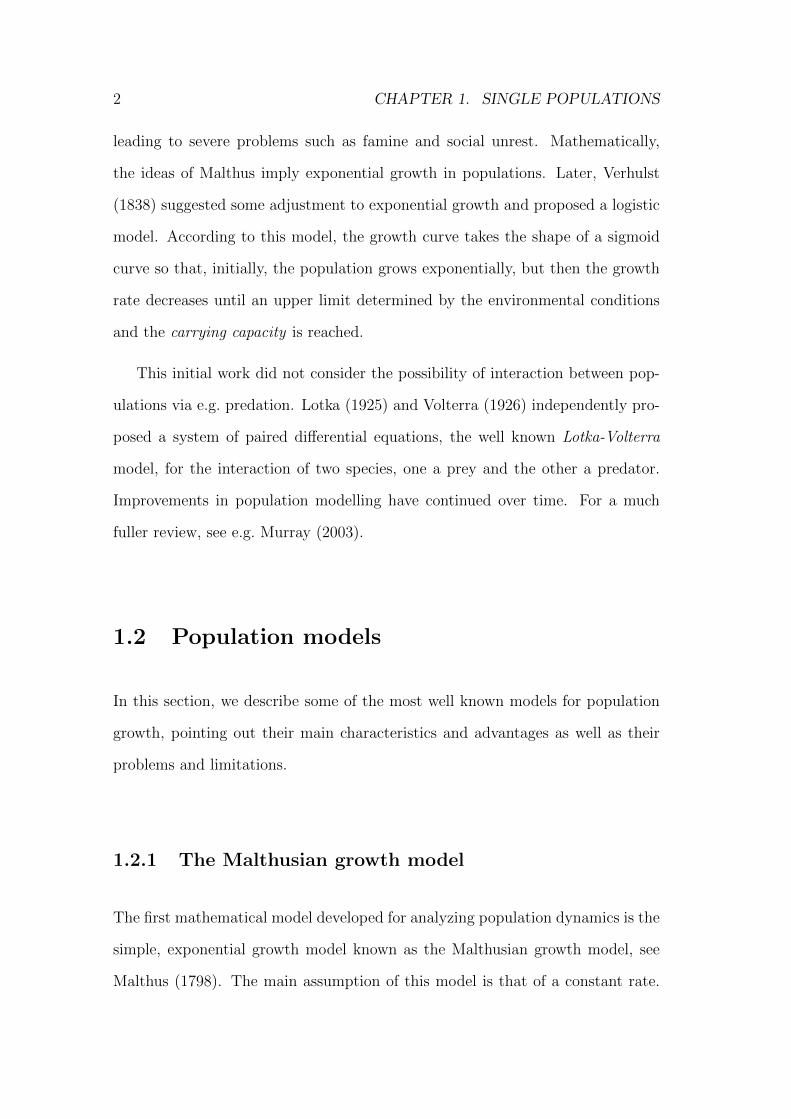
leading to severe problems such as famine and social unrest. Mathematically,
the ideas of Malthus imply exponential growth in populations. Later, Verhulst
(1838) suggested some adjustment to exponential growth and proposed a logistic
model. According to this model, the growth curve takes the shape of a sigmoid
curve so that, initially, the population grows exponentially, but then the growth
rate decreases until an upper limit determined by the environmental conditions
and the carrying capacity is reached.
This initial work did not consider the possibility of interaction between pop-
ulations via e.g. predation. Lotka (1925) and Volterra (1926) independently pro-
posed a system of paired differential equations, the well known Lotka-Volterra
model, for the interaction of two species, one a prey and the other a predator.
Improvements in population modelling have continued over time. For a much
fuller review, see e.g. Murray (2003).
1.2 Population models
In this section, we describe some of the most well known models for population
growth, pointing out their main characteristics and advantages as well as their
problems and limitations.
1.2.1 The Malthusian growth model
The first mathematical model developed for analyzing population dynamics is the
simple, exponential growth model known as the Malthusian growth model, see
Malthus (1798). The main assumption of this model is that of a constant rate.

1.2. POPULATION MODELS 3
The model can be represented by the following differential equation,
dN
dt= rN, (1.1)
where at time t, N = N(t) is the population size and r = b − d is the constant
growth rate, equal to the difference between the constant birth and death rates
(b and d respectively).1 The solution to the differential equation (1.1) is
N(t) = N0ert = N0e
(b−d)t, (1.2)
where N0 = N(0) is the initial population size at time zero. If the birth rate is
greater than the death rate, that is if b > d, then r > 0 and the population grows
exponentially while if b < d, then r < 0 and the population decreases exponen-
tially till it dies out. Finally, if b = d, then the population remains constant at its
initial level. Figure 1.1 shows how the speed of the population growth depends
on the value of r. Notice that at time 10, the size of the population represented
by the dashed line is more than twice the population size represented by the solid
line while the difference in the value of r is only one tenth.
The kind of growth represented by the Malthusian model is possible only under
special conditions. For instance, bacteria grow by simple division, so that in an
experiment under ideal conditions for reproduction, with plenty of food and lack
of predators, it is possible to observe exponential growth. However, in practice
even bacteria do not grow indefinitely as eventually, food supplies grow short and
reproduction conditions deteriorate. This is the main disadvantage of this model.
Nevertheless, the model is very simple and can be useful for predictions in the
very short time.
1For this reason this model is also called the pure birth-death process model.

4 CHAPTER 1. SINGLE POPULATIONS
Figure 1.1: Exponential Growth
1.2.2 The logistic growth model
To overcome the problems of the Malthusian model, some adjustments are neces-
sary. Verhulst (1838) proposed a new model where the population has a maximum
size. Under this approach, the population growth rate depends not only on the
current population size, but also on how far this is from a fixed upper limit. This
maximum population size can reach is called the carrying capacity of the environ-
ment and depends on the availability of resources. Formally, Verhulst’s logistic
growth model is defined by the following differential equation:
dN
dt= rN(1− N
K), where r,K > 0, (1.3)
where r is the growth rate and K is the carrying capacity. This equation is in-
tended to capture two features. Firstly, when the population size is small, then
the Verhulst model is close to the Malthusian model so that growth is approxi-
mately exponential. Secondly, when the population is large, starvation occurs so
that the growth rate decreases as the population size gets closer to the carrying
capacity. Thus, if the population size is far from this maximum, it would grow

1.2. POPULATION MODELS 5
quickly, but as it approaches the carrying capacity the growth rate slows down.
The solution of Equation (1.3) is:
N(t) =KN0e
rt
K +N0(ert − 1), (1.4)
where N0 is the initial population size as earlier. Note that for r > 0, then
limt→∞N(t) = K so that the population tends to the upper limit as time in-
creases. For r < 0 the population eventually dies out and for r = 0, the popula-
tion remains at its initial size as for the Malthusian model.
Figure 1.2 shows the curve produced by the logistic equation. This is an
S-shaped or sigmoidal curve. Initially the population grows exponentially but,
when the population size is closer to the carrying capacity, growth decelerates
until the stable upper bound is reached.
Figure 1.2: Logistic Growth
The logistic growth model describes the self-limiting growth of a population
where the growth process depends on the population density. When the pop-
ulation size increases, individuals start to compete with other members of the
population for food and other critical resources. This is the so-called bottleneck

6 CHAPTER 1. SINGLE POPULATIONS
effect. Nevertheless, the problem with this model is the difficulty of knowing the
true value of K in a given habitat. Even when this value is known, at a given
moment, it might not be constant and may change over time. Another limitation
is that the population dynamics are often more complex than can be captured by
this model. For instance, the age of the individuals is not taken into account and
this can be an important factor as often, the capacity of reproduction depends
on age.
1.2.3 Delay models
The two models considered thus far can be included in a more general class of
models, specified by the differential equation
dN
dt= f(N)N, (1.5)
where f(N) is the specific growth rate. If f(N) is a constant, then differential
equation (1.5) leads to Malthusian, pure exponential growth while, if f(N) =
r(1−N/K) we have the Verhulst, logistic growth model. An important problem
with these models is that they assume that the reproductive capacity of the
population individuals is independent of their age. In particular, many species
need to grow to a certain age or undergo a gestation period before they are capable
of reproduction. This suggests the incorporation of a time delay. To take into
account this feature, the differential equation (1.5) may be modified to become
dN
dt= f(N−T )N, (1.6)
where T is a positive constant and represents the delay parameter and at time
t, N−T represents N(t − T ). Equation (1.6) shows that the population is now a

1.2. POPULATION MODELS 7
function of the current populations and the population T periods before. This
new model is a little bit more realistic than the previous ones, but a better model
for a delay effect should really be an average over all past populations.
1.2.4 Models for interacting populations
Species are not usually alone in their habitat and on the contrary, usually there are
various species interacting in the same habitat so that the population dynamics of
each species are affected by the interrelationship among them. From e.g. Murray
(2003), there are three main types of interaction:
i) If the density of one population decreases while the other increases, the
populations are in a predator- prey situation.
ii) If the growth rates of both populations decrease simultaneously, then there
is competition.
iii) If the growth rates of both populations increase simultaneously then this is
called mutualism or symbiosis.
Here, we will outline a particular model for predator-prey interactions, that
is the Lotka-Volterra equations developed in Lotka (1925) and Volterra (1926).
Under this model, when the predators population increases, the prey population
decreases and as the predator population falls, the prey population increases.
These dynamics continue in a cycle of growth and decline. The system of differ-
ential equations that model this behaviour is:
dN
dt= N(a− bP ) (1.7)
dP
dt= P (cN − d), (1.8)

8 CHAPTER 1. SINGLE POPULATIONS
where N = N(t) is the prey population, P = P (t) is the predator population
and a, b, c and d are positive constants. This model assumes that the prey has
an unlimited food supply so that in the absence of predation the prey population
grows exponentially as in the Malthusian model. When predation occurs, this
reduces the prey growth rate in proportion to the product of the current prey
and predator populations, as can be seen in the last term of Equation (1.7).
The change in the prey population is given by its own growth minus the rate
at which it is preyed upon. On the other hand, in the absence of any prey
for sustenance the predator population decays exponentially. Finally, the prey
contribution to the predator growth rate is proportional to the available prey and
predator populations, bNP . The change in the predator population is the growth
of the predator population minus natural death.
Equilibrium occurs in this model when both population levels are not chang-
ing. Setting both differential equations, (1.7) and (1.8), equal to zero and solving,
we get two equilibria: first at N = P = 0, and second at N = d/c and P = a/b.
The first solution represents the extinction of both species. If both population
levels are at 0, then they will continue to be so indefinitely. The level of the
second solution depends on the parameter values. Due to the fact that all the
parameters are restricted to be positive, then at this second equilibrium both
populations sustain their current non-zero size and do so indefinitely.
Figure 1.3 shows the phase trajectories. As we can see, the trajectories in
the in the N − P phase plane are closed lines with elliptical shape. For each
possible set of initial conditions, N0 = N(0) and P0 = P (0), there is a closed
orbit with amplitude determined by the starting point. In order to analyzes the
predator-prey phase space is useful divide the graph into four regions by the

1.2. POPULATION MODELS 9
Figure 1.3: Phase plane trajectories of the Lotka-Volterra model
equilibrium (N = d/c and P = a/b).2 In the first region, both populations grow.
In the second region, predator population grows and therefore, the number of
prey declines. In the third region, both populations decline and in the last region
predators still declining while prey population starts to grow. A closed trajectory
like this in the phase plane implies periodic solutions in t for N and P in (1.7)
and (1.8).
One of the limitations of the Lotka-Volterra model is that it is not very re-
alistic and hence context specific information must be added. The model does
not consider any competition for resources among prey or predators and, as a
consequence, the prey population may grow infinitely. On the other hand, preda-
tors have no saturation, they consumption rate is unlimited and proportional to
the prey density. Therefore, the model behaviour shows no asymptotic stability
and neither equilibrium point is stable. Instead, the predator and prey popula-
tions cycle endlessly. This cyclic behaviour has been observed in nature but it is
not very common. The Lotka-Volterra model is insufficient for modelling many
2In our example a = 0.1, b = 0.01, c = 0.001 and d = 0.05. Then the equilibrium is atN = 50 and P = 10.

10 CHAPTER 1. SINGLE POPULATIONS
predator-prey systems.
A more general formulation of this model which resolves some of these prob-
lems assumes that the growth functions may be non-linear
dN
dt= f(N,P )N (1.9)
dP
dt= g(N,P )P, (1.10)
where f and g represent the per capita growth rates of the prey and predator,
respectively.
1.2.5 Stochastic models
Population dynamics are complex systems because different factors may affect
the populations. Some of these factors can be modelled explicitly but in other
cases we cannot model such factors. Nevertheless, it is necessary to include their
effects in these population models. One way to do this is to include random
variables that account for the collective influence of such factors.
Models in population dynamics include three basic forms of randomness or
stochasticity (see Lande et al. (2003)): demographic stochasticity, environmen-
tal stochasticity, and sampling error. The first one refers to chance events of
individual mortality and reproduction. At a moment of time, an individual can
die with a certain probability, and this probability is usually conceived as being
independent among individuals. This kind of stochasticity tends to have greater
effect in small populations than in large populations. Environmental stochas-
ticity refers to temporal fluctuations in the probability of the mortality and the
reproductive rate of all individuals in a population. An extreme example are

1.2. POPULATION MODELS 11
the unpredictable catastrophes like fire, flood, hurricane, epidemic, etc. The last
source of stochasticity arises from sampling procedure.
Thus, dynamics of populations has both deterministic and stochastic com-
ponents that operate simultaneously. According to Turchin (2003), there are at
least three different ways to include the stochasticity. The most direct approach,
when data are observed at regular, discrete time points, say t = 0, 1, 2, . . ., is to
add noise to the population rate of change, that is:
rt+1 = f(Zt) + εt, (1.11)
where rt+1 = log(Nt+1/Nt), Zt is the vector of state variables and εt is a random
variable with some probability distribution. Noise is included in additive manner
because environmental fluctuations are likely to affect per capita death and birth
rates, and these rates are combined additively in determining rt+1.
A second approach to including stochasticity in the model is to add a random
component directly to Nt. One possible mechanism that supports this approach
is the inclusion of random immigration events. Finally, the third approach is
to randomly vary the parameters of the model. This approach is useful when
researchers know in which part of the population process environmental effects
are the most important.
As an example consider the following extension of the Lotka-Volterra model
proposed by Gilioli et al. (2008). They initially consider a modified predator-prey
system that takes into account the intra-specific prey competition as follows:
dN = [aN(1−N)− bNP ]dt (1.12)
dP = [cbNP − dP ]dt, (1.13)

12 CHAPTER 1. SINGLE POPULATIONS
where N = N(t) and P = P (t) are the biomass of prey and predator at time t per
spatial unit normalized with respect to carrying capacity, a is the specific growth
rate of the prey, b is a positive constant representing the rate of effective search
per predator, c is the maximum specific production rate of the predator and d
is the specific loss rate of predator due to natural mortality. The parameters
a, c and d are known, as well as the initial values (N0, P0). The behavioural
parameter b is unknown. A stochastic extension of this model is formulated by
including both demographic and environmental stochasticity factors, which are
assumed independent. The demographic stochasticity is included by modifying
the parameter b:
b(t) = b(0) + σξ(t), (1.14)
where ξ(t) is Gaussian white noise, so that b fluctuates around its mean value. 3
Substituting (1.14) in (1.12) and (1.13) the model becomes:
dN = [aN(1−N)− b0NP ]dt− σNPdw1 (1.15)
dP = [cb0NP − dP ]dt+ cσNPdw1 (1.16)
where b0 = b(0) and w1 is a Wiener process. Environmental stochasticity is sup-
posed to affect both predator and prey populations because they share the same
habitat. The effect of this factor is included by an additive noise depending on
each population density. Finally, the proposed stochastic Lotka-Volterra system
is
dN = [aN(1−N)− b0NP ]dt− σNPdw1 + εNdw2 (1.17)
dP = [cb0NP − dP ]dt+ cσNPdw1 + ηPdw2, (1.18)
3It is assumed that mean and variance fixed are such way that the random variable canrarely take negative values.

1.3. BACTERIAL GROWTH MODELS 13
where w2(t) is a Wiener process independent from w1(t) and ε and η are two
positive parameters.
1.3 Bacterial growth models
In the field of predictive microbiology the concept of the primary model is fun-
damental. A primary model describes the kinetics of the growth process by
parameters having a biological interpretation. The population size is a function
of time and the model aims to describes the different stages of growing.
Bacterial growth is the division of one bacterium into two, identical, daughter
cells during a process called binary fission. Both daughter cells do not necessarily
survive but if the number of surviving cells is, on average, greater than a half,
then the bacterial population grows exponentially. Figure 1.4 shows the typical
behaviour of bacterial density along the time. Bacterial growth in batch culture
experiments where an initial population is planted in a petri dish containing
nutrients and then growth is observed over time, can usually be divided in four
different phases:
i) In the lag phase bacteria adapt themselves to growth conditions. Individual
bacteria are not yet able to divide, they are maturing.
ii) The exponential phase is the cell doubling period. The number of new
bacteria per unit time is proportional to the present population.
iii) During the stationary phase, the growth rate slows down as a consequence
of nutrient depletion and accumulation of wastes. This phase is reached as
the bacteria begin to exhaust the limited resources available to them.

14 CHAPTER 1. SINGLE POPULATIONS
iv) The final phase is the death phase. There are no nutrients left and the
bacteria die.
Figure 1.4: Stages of bacterial growth
Given this type of behaviour we can model bacterial growth in the first three
phases with a sigmoidal function which represents the different stages of grow-
ing. In addition to the logistic model, the most widely used deterministic, para-
metric bacterial growth models are the Gompertz, (Gompertz (1825)) Baranyi
(Baranyi and Roberts (1994), Baranyi and Roberts (1995)) and Buchanan mod-
els (Buchanan et al. (1997)) which are outlined below.
1.3.1 Gompertz model
The Gompertz function, introduced in 1825, originated in the field of actuarial
science. Gompertz proposed the following equation for the number of survivals
of a population at any age t,
N(t) = aebe−ct
(1.19)
where a > 0 is the upper asymptote, b < 0 is a constant and c > 0 is a positive
constant related with the growth rate. After some years, the Gompertz equation
1.3. BACTERIAL GROWTH MODELS 15
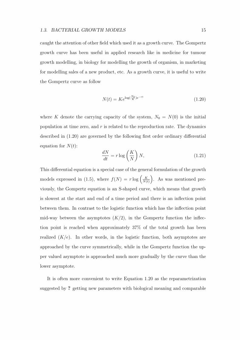
caught the attention of other field which used it as a growth curve. The Gompertz
growth curve has been useful in applied research like in medicine for tumour
growth modelling, in biology for modelling the growth of organism, in marketing
for modelling sales of a new product, etc. As a growth curve, it is useful to write
the Gompertz curve as follow
N(t) = Kelog(N0K
)e−rt
(1.20)
where K denote the carrying capacity of the system, N0 = N(0) is the initial
population at time zero, and r is related to the reproduction rate. The dynamics
described in (1.20) are governed by the following first order ordinary differential
equation for N(t):
dN
dt= r log
(K
N
)N, (1.21)
This differential equation is a special case of the general formulation of the growth
models expressed in (1.5), where f(N) = r log(
KN(t)
). As was mentioned pre-
viously, the Gompertz equation is an S-shaped curve, which means that growth
is slowest at the start and end of a time period and there is an inflection point
between them. In contrast to the logistic function which has the inflection point
mid-way between the asymptotes (K/2), in the Gompertz function the inflec-
tion point is reached when approximately 37% of the total growth has been
realized (K/e). In other words, in the logistic function, both asymptotes are
approached by the curve symmetrically, while in the Gompertz function the up-
per valued asymptote is approached much more gradually by the curve than the
lower asymptote.
It is often more convenient to write Equation 1.20 as the reparametrization
suggested by ? getting new parameters with biological meaning and comparable

16 CHAPTER 1. SINGLE POPULATIONS
with the other models and known as the modified Gompertz equation,
N(t) = N0 + (Nmax −N0) exp(− exp(µmax exp(λ− t)
(Nmax −N0) log(10)+ 1)) (1.22)
where λ is the lag time, µmax is the maximum specific growth rate and Nmax is
the maximum population density.
1.3.2 Baranyi model
The modified Gompertz equation and the logistic function were not originally
developed by modelling bacterial growth and therefore are considered as purely
empirical models. In a series of papers, see e.g. Baranyi and Roberts (1994),
Baranyi and Roberts (1995), Baranyi et al. (1999), Baranyi and co-workers de-
veloped a mechanistic model for bacterial growth putting special attention to the
lag phase which is attributed to the need to synthesize an unknown substrate
q critical for growth. The Baranyi model is different from the previous one be-
cause it includes a new term, g(t), called the adjustment function. This function
describes the adjustment of the culture to the new environment and it affects
the course of growth before the exponential phase. In a typical batch culture
experiment the bacterial population is first cultured under more or less optimal
conditions and then inoculated and grown in a new environment. The authors
argue that the physiological state at t = 0 affects the length of the lag period
in the new environment. The lag in the post-inoculation environment is longer
if the cells are closer to the stationary phase in the pre-inoculation environment.
In a general formulation, the new model describes the bacterial batch culture by
means of the differential equation
dN
dt= g(t)f(N)N, (1.23)

1.3. BACTERIAL GROWTH MODELS 17
with f(N) = µmax
(1− N(t)
Nmax
)and g(t) = q0
q0+et, being µmax the maximum specific
growth rate, Nmax the maximum population density and q0 the physiological state
of the inoculum.
The explicit form of the model is the following
N(t) = N0 + µmaxA(t)− log(1 +eµmaxA(t) − 1
e(Nmax−N0) (1.24)
A(t) = t+1
vlog(
e−µmaxt + q0
1 + q0
) (1.25)
with the same parameters as earlier. The more familiar lag time, λ, could be
calculated from the values of q0 and µmax as
λ =log(1 + 1
q0)
µmax(1.26)
Then, the growth equation was reparametrized by Wilson (1999) in terms of the
lag time. The new form is given by:
N(t) = N0 +N1
log(10)− N2
log(10)(1.27)
where
N1 = µmaxt+ log(e−µmaxt − e−µmax(t+λ) + e−µmaxλ) (1.28)
N2 = log(1 + 10(N0−Nmax)(eµmax(t−λ) − e−µmaxλ)) (1.29)
In this form the Baranyi equation is expressed in terms of more familiar quanti-
ties with intuitive biological interpretations. Since its introduction, the Baranyi
model has been used extensively to model the growth of a wide variety of mi-
croorganisms.

18 CHAPTER 1. SINGLE POPULATIONS
1.3.3 Three phase linear model
An alternative model was proposed in Buchanan et al. (1997). This model is a
three-phase linear model where each phase describes one of the bacterial growth
stages: lag, exponential and stationary, see Figure 1.5. As, during the lag phase
bacteria are adapting to the new environment the model assumes that the growth
rate is equal to zero. Once the bacteria are adapted, they begin to divide and
in the exponential growth phase the model assumes a constant growth rate, with
the log of the density population increasing linearly with time. Finally, when the
stationary phase is reached, the growth rate returns to zero. The model can be
formalized as:
N(t) = N0 for t ≤ tlag (1.30)
N(t) = N0 + µ(t− tlag) for tlag < t < tmax (1.31)
N(t) = Nmax for t ≥ tmax (1.32)
where N(t) is the log of the population density at time t, N0 the log of the initial
population density, Nmax the log of the maximum population density supported
by the environment, t the elapsed time, tlag the time when the lag phase ends,
tmax the time when the maximum population density is reached and µ the specific
growth rate. Despite its simplicity, this model has not been as widely used for
fitting growth data as the Gompertz and Baranyi models introduced earlier.

1.3. BACTERIAL GROWTH MODELS 19
Figure 1.5: Graphical representation of the Buchanan model
1.3.4 Secondary models
Traditionally, primary growth models are developed for static environmental con-
ditions, however reality is characterized by changing environmental conditions.
Secondary models are developed to describe the effect of environmental conditions
such as, temperature, pH, salinity, water activity, on the values of the growth pa-
rameters of a primary model. Most of the secondary models can be divided
into one of three categories, that is square root, polynomial and cardinal mod-
els. Firstly, square root models describe the effect of suboptimal temperature on
growth rate of microorganisms see e.g. Ratkowsky et al. (1982). Secondly, poly-
nomial models allow any of the environmental factors and their interactions to be
taken into account and were extensively used in the 1990s. However, these models
include an excessive number of parameters with lack biological interpretability.
Rosso et al. (1993) introduced a model that described the influence of temper-
ature, acidity level and water activity on the growth rate based on the gamma
concept and using only parameters that were biologically significant. This model
then became widely known as the cardinal model. In Chapter 3, secondary models
will be presented in more detail.

20 CHAPTER 1. SINGLE POPULATIONS
1.4 Model fitting
Most of the growth models presented previously, and, in particular, the logistic
function, the Baranyi and the Gompertz equations, are nonlinear growth models.
These were presented as deterministic parametric models, where the parameters
have meaningful biological interpretations and the functional form represents the
underlying behaviour in the growth system. Assuming that data are observed at a
set of equally spaced time points, then by adding an error term, the deterministic
model is replaced by a statistical model. In general notation, these models can
be expressed as
yi = f(xi,θ) + εi (i=1,2,. . . ,n), (1.33)
where yi is the ith observation of the dependent variable, f is a (nonlinear) func-
tion, xi are the ith observations of the independent variables, θ is the vector of
parameters and the error terms, εi, have zero mean.
To fit the curve, sometimes it is possible to transform the nonlinear model
in a linear one. This kind of models are called transformably linear or “intrinsi-
cally linear”. The advantage to apply this transformation relies on that with a
linearized model we can apply standard linear regression methods. Additionally,
depending on the structure of the errors, transformation to linearity could also
achieve errors approximately normally distributed and with constant variance.
Nevertheless, parameters of the transformed model are not as interesting or as
important as the original parameters and usually they are difficult to interpret.
1.4.1 Nonlinear Least Squares
As in linear regression, parameters of interest can be estimated by the method
of least squares. The least squares estimate of θ, denoted by θ, it is obtained

1.4. MODEL FITTING 21
minimizing the error sum of squares,
S(θ) =n∑i=1
[yi − f(x,θ)]2. (1.34)
Assuming that errors are independent and identically distributed with zero mean
and constant variance, θ is an asymptotically unbiased estimate of the parameter
vector θ. Under certain regularity assumptions θ is also asymptotically normally
distributed as n→∞. Additionally, if it is assumed that the errors are normally
distributed, then θ is also the maximum-likelihood estimator. For more details
see Seber and Wild (1989).
This minimization problem yields normal equations that are nonlinear in the
parameters and therefore they can not be solved analytically for most of the mod-
els. Therefore, in order to provide approximate, analytic solutions it is necessary
to employ iterative methods.
Approximating the model by the first-order Taylor series expansion, yields
the vector of parameter estimates: b = (J′J)−1J′y; being J the Jacobian matrix
which contains the derivatives of the model with respect to the parameters and
evaluated in the n points. An estimate of the covariance matrix V of the param-
eter estimates can be computed as V = (J′J)−1σ2, where σ2 is the error variance.
This method will converge fast provided the neighbourhood of the true parameter
values has been reached. However, if the initial parameter values are too faraway,
the convergence would never be reached. Alternative iterative procedures could
be applied such as the steepest descent method and the Levenberg-Marquardt’s
method. The former method is able to converge even though initial values are far
removed from the true parameter values, but the asymptotic rate of convergence
is very slow. The Levenberg-Marquardt (Levenberg (1944),Marquardt (1963))
method is the most widely used method of computing nonlinear least squares es-

22 CHAPTER 1. SINGLE POPULATIONS
timators and most standard statistical packages contain computer routines to fit
nonlinear regression models using this algorithm. This method is a compromise
between the linearization and the gradient methods. It almost always converges
and the convergence rate does not slow down at the later stages of the iterative
procedure.
A number of software packages are available for fitting the various bacterial
growth models previously described using these techniques. In particular, the
grofit package for R available from
http://cran.r-project.org/web/packages/grofit/index.html
can be used to fit the logistic, Gompertz and modified Gompertz models among
others. In the case of the Baranyi model, software includes DMFit, for Microsoft
Excel, available from
http://www.combase.cc/index.php/en/downloads/category/11-dmfit
and MicroFit, a stand alone package distributed by the Institute of Food Re-
search in the U.K which can be obtained from
http://www.ifr.ac.uk/microfit/.
1.4.2 Bayesian estimation
As we have seen, classical statistical methods for nonlinear regression are based on
linearization of the nonlinear models around the unknown parameter. Typically,
the distribution of the least squares parameter estimators is known only asymp-
totically and these asymptotic approximations may be inadequate in practice for
small-sample problems. Assuming that the error distribution of the nonlinear
model is known, an alternative procedure which does not rely on the lineariza-
tion of the model is to use a Bayesian approach where asymptotic theory is
not involved. The Bayesian approach assumes that the parameters are random

1.4. MODEL FITTING 23
variables instead of unknown constants, that is the parameters themselves have
some unknown probability distribution. The approach relies on the idea that re-
searches have some prior beliefs or knowledge about the system under study and
this knowledge is updated once the data are observed. The inclusion of readily
accepted prior information is particularly useful when the sample size is small.
Consider the nonlinear model (1.33) in vector form,
y = f(θ) + ε (1.35)
Bayesian models are constructed by specifying the conditional distribution of the
observable variable y (data) given the model parameters θ, that is p(y|θ), and
a prior distribution for these parameters, p(θ) which expresses the current level
of uncertainty before any data are observed. Once data are observed, inference
about the parameters is based on the posterior distribution p(θ|y). Using Bayes
Theorem, this is calculated as:
p(θ|y) =p(y|θ)p(θ)
p(y)
∝ p(y|θ)p(θ)
so that the posterior parameter distribution, p(θ|y), is proportional to the prod-
uct of the likelihood function, p(y|θ) and the prior distribution of the parameters
p(θ). The posterior distribution is a joint probability distribution of all model
parameters and point estimates or uncertainty intervals can be obtained from it.
For good general reviews of the Bayesian approach in ecological modeling see e.g.
McCarthy (2007), King et al. (2009).
The computation of the exact conditional posterior distributions is most often
impossible. In such cases, Markov-Chain Monte-Carlo (MCMC) techniques can

24 CHAPTER 1. SINGLE POPULATIONS
be applied to generate samples from the posterior distributions. This method
generates chains of simulated values for parameters, with the sampling distribu-
tion converging to the relevant posterior distribution. The freeware computer
package WinBUGS, see Lunn et al. (2000) is a powerful and flexible tools able to
implement these chains for a wide range of possible models. In the next section,
we show how a Bayesian approach can be implemented to make inference for the
growth models using WinBUGS.
1.5 Growth curve modeling using WinBUGS
In Section 1.4.1 we commented on a number of packages for fitting growth models
using non-linear least squares approaches. However, to the best of our knowledge,
thus far, no general computational package has been developed for the implemen-
tation of Bayesian inference in bacterial growth models. For that reason, in this
section we describe the use of WinBUGS, in the context of bacterial growth. For a
full review of WinBUGS in the context of ecological modeling, see e.g. Kery (2010).
1.5.1 Model specification
Assume that population density data Nt = N(t), are observed at a set of reg-
ular time points, say t = 0, 1, . . . , T . Then, a model specification must be
assumed. For illustration, consider the modified Gompertz equation, where
Nt = g(N0, Nmax, µmax, λ, t) where g is the function defined in (1.22) with four
parameters: N0 is the initial population density, Nmax the maximum population
size, µmax is the maximum growth rate and λ is the lag period. Then, a sample
distribution for the error term must be assumed. Suppose that the errors are
independent and identically normally distributed with variance σ2, so that we

1.5. GROWTH CURVE MODELING USING WINBUGS 25
have:
Nt ∼ N (g(N0, Nmax, µmax, λ, t), σ2). (1.36)
The model specification is completed by assigning prior distributions for the
model parameters. A possible structure of prior distributions is:
logN0 ∼ N (µN0 , σN0)
logNmax ∼ N (µNm , σNm)
log µmax ∼ N (µµ, σµ)
log λ ∼ N (µλ, σλ)
where µi and σi are the mean and the standard deviation of the natural logarithm
of the parameter i. The parameters of the prior distributions are chosen in such
a way that they reflect the prior knowledge about the model parameters. The
source of information could come from the opinion of an expert and / or the results
of previous studies. If there is no reliable previous information, it is better to
used non-informative prior distributions, that is priors with high variance which
reflect the uncertainty about model parameters. We follow this approach and
set the means of the prior distributions equal to zero and the variances equal
to 100. Finally, the prior distribution of the error variance is an inverse gamma
distribution, 1/σ2 ∼ G(a, b).
The dependence structure represented by this model and prior is represented
in Figure 1.6. In the figure, called a doodle in WinBUGS, random and logical nodes
are represented by ellipses and fixed nodes (independent variables) are represented
by rectangles. The arrows represent dependence relationships with the single
arrows showing stochastic dependence and the double arrows representing logical
dependence.

26 CHAPTER 1. SINGLE POPULATIONS
Figure 1.6: The dependence structure of the modified Gompertz model
The following WinBUGS code to represent the model specification can be gen-
erated from the doodle or programmed directly:
model
for(i in 1:n)
g[i] <- N0 + (Nmax-N0)* exp(-exp(((mu*exp(1)*(lambda-t[i]))/
((Nmax-N0)*log(10)))+1))
N[i] ~ dnorm(g[i], tau)
N0 ~ dlnorm(0, 0.01)
Nmax ~ dlnorm(0, 0.01)
lambda ~ dlnorm(0, 0.01)
mu ~ dlnorm(0, 0.01)
tau ~ dgamma(0.01,0.01)
where n is the number of observations. As the population size, the growth rate
and the lag period are non-negative quantities, we used lognormal prior distri-
butions, but alternative distributions can be used, such as the truncated normal
distribution

1.5. GROWTH CURVE MODELING USING WINBUGS 27
mu ~ djl.dnorm.trunc((0,0.01,0,1000)
or the gamma distribution
mu ~ dgamma(0.01, 0.01).
Note that WinBUGS requires the specification of the precision (τ = 1/σ2) in-
stead of the variance. This is not a problem however as a helpful feature of
WinBUGS is the use of logical relationships to define functions of the parameters
in the model. For example, to calculate the variance, it is enough to define
sigma2 <- 1 / tau
which allows inference for the variance parameter to be undertaken.
In the field of microbiology, a very useful quantity of interest in is the doubling
time, also called generation time. Doubling time is the time it takes a bacterium
to do one binary fission starting from having just divided. That is looking at the
all population, it is the period of time required for the population to double in
size. Then, generation time is can be computed as the natural logarithm of 2
divided by the growth rate. Calling gt the generation time, the code for compute
it in WinBUGS in our example is
gt <- log(2) / mu
After the model code has been checked, the data must be loaded in S-Plus
format or, for data in arrays, in rectangular format. For instance, in our Gompertz
example, we need to specify the sample size, n, the vector with the observations
of the population size N and the vector of the corresponding observations times
t, both of length n. This is achieved as follows:

28 CHAPTER 1. SINGLE POPULATIONS
list(
n = 16,
t = c( 0, 1, 2, 3, 4, 5, 6, 7, 8, 9, 10, 11, 12, 13, 14, 15),
N = c( 0.07, 0.07, 0.08, 0.09, 0.14, 0.31, 0.52, 0.74, 0.85, 0.88, 0.90, 0.92,
0.94, 0.95, 0.96, 0.96)
)
Finally, we need to specify the initial values for the variables to be estimated.
The format for introducing this information is the same as for the data. In our
example,
list(N0 = 0.07, Nmax = 1, lambda = 4, mu = 0.25, tau = 1)
Alternatively, it is possible to use the WinBUGS generator of initial values,
which are drawn from the prior distributions (or from an approximation to the
prior). Nevertheless, when vague prior distributions are used, it is not appropriate
to use this generator as the values generated could be very improbable.
After that, the model is run until convergence is reached. Convergence can
be checked in WinBUGS by looking at the trace of the sample values generated
at each iterations to see if the chain seems to be stabilized. Additionally, the
Gelman-Rubin statistic (Gelman and Rubin (1992), Brooks and Gelman (1998))
can be computed for what run several chains is needed. Finally, it is important
to check the autocorrelation of the MCMC sampled data which, for example, can
be done using simple autocorrelation plots. If there is autocorrelation up to lag
5 say, the data can be thinned by taking just every fifth datum to produce an
approximately independent sample.
A standard session in WinBUGS can be resumed as follows. Firstly, the model is
specified in the form of the likelihood and prior distributions for all the unknown

1.5. GROWTH CURVE MODELING USING WINBUGS 29
model parameters. Secondly, data and initial values are loaded. Finally the model
is run and assuming convergence, the generated MCMC simulations are a sample
from the posterior distributions of interest.
1.5.2 Data analysis
Useful summary statistics and graphical representations of the posterior distri-
butions can easily be obtained in WinBUGS trough the Sample Monitor Tool. The
posterior mean, standard devitation and quantiles, as well as plots of smooth
kernel density estimate or trace for the parameters are outputs that WinBUGS
provides to summarize the posterior distribution.
1.5.3 Model comparison
A widely used statistic for comparing models in a Bayesian framework is the
Deviance Information Criterion (DIC) of Spiegelhalter et al. (2002). This criterion
penalizes actions for departure from the corresponding observed value as well
as for the number of parameters in the model. In this way, the approach is
a compromise between goodness of fit and model complexity. The DIC is easily
calculated from the samples generated by a Markov chain Monte Carlo simulation
and is implemented automatically in WinBUGS. Formally, for a model with data
y and parameters θ, the DIC is equal to
DIC = pD +D(θ) (1.37)
where D(θ) = −2 log(p(y|θ)) is the deviance and D(θ) is the posterior mean of
the deviance, approximated by∑m
i=1 = θi (m is the number of iterations). The
expected deviation measures how well the model fits the data. The lower is, the

30 CHAPTER 1. SINGLE POPULATIONS
better the fit. The effective number of parameters, pD, computed as the difference
between the measure of fit and the deviance at the estimates D(θ) − D(θ) is a
measure of model complexity, roughly speaking the number of parameters in the
model. Lower values of the criterion indicate better fitting models. More details
about the DIC can be found in Spiegelhalter et al. (2002).
1.6 Application: Listeria monocytongenes
Listeria is a bacterial genus containing six species. These species are Gram-
positive bacilli and are typified by listeria monocytogenes. This bacteria is a
well-known food-borne pathogen (rarely but fatally infectious as listeriosis) and
is commonly found in soil, stream water, sewage, plants, and food. The serious
health and economic consequences of listeriosis have lead to a wide amount of
studies of this bacteria, see e.g. Augustin and Carlier (2000), Delignette-Muller
et al. (2006), Pouillot et al. (2003) and Powell et al. (2006) among others. In our
application the models are fitted to listeria growth curves. The data come from
an experiment in broth monoculture. The environmental conditions remained the
same for the curve, which was generated at 42 , pH=7,4 and 2,5% NaCl (salt
concentration). The data set consists of 16 observations.
Classical inference
Figure 1.7 shows the growth data and the fitted curves for two general growth
models discussed previously, that is the Malthusian model and the logistic model.
The Malthusian model was fitting taking into account only the data corresponding
to the exponential phase of growth and the logistic model was fitting to all the
observations. The Malthusian model fits the first part of the data well, but cannot

1.6. APPLICATION: LISTERIA MONOCYTONGENES 31
explain the stationary phase of the bacterial growth.
(a) Malthusian model (b) Logistic model
Figure 1.7: Growth models fitted to the Listeria growth data
In contrast, the logistic model fits the data on the exponential and stationary
phases, but fails to explain the lag phase. To overcome these problems, we also
fitted the Baranyi and Gompertz models to these data.4 Figure 1.8 shows the
new fitted curves and Table 1.1 summarizes the results of the estimation.
Figure 1.8: Baranyi and Gompertz models fitted to the Listeria growth curve
4These models were fitted to the data using the nlstools package of R. Note that we considerthe log to base ten of the cell concentration

32 CHAPTER 1. SINGLE POPULATIONS
Table 1.1: Baranyi and Gompertz Parameters
Estimate Std. Error 2.50% 97.50% P-valueBaranyi’s model:λ 3.804 0.063 3.666 3.943 3.05E-16 ***µmax 1.246 0.044 1.150 1.342 2.35E-12 ***N0 -1.149 0.009 -1.169 -1.129 2.00E-16 ***Nmax -0.032 0.005 -0.044 -0.021 4.93E-05 ***RSE 0.014Gompertz’s model:λ 3.087 0.058 2.960 3.214 1.34E-15 ***µmax 0.747 0.021 0.702 0.792 1.29E-13 ***N0 -1.126 0.007 -1.142 -1.111 2.00E-16 ***Nmax -0.022 0.005 -0.033 -0.011 0.00109 **RSE 0.013*** : α = 0.01 and ** : α = 0.05
We can observe that both models fit the experimental data well, with the
greatest differences being observed during the transition periods, from lag to
exponential phase and from the last one and the stationary phase. Analyzing
the residual standard errors, we can see that Gompertz model fits a little bit
better than Baranyi model. Regarding the parameter estimates, both models
yields statistically significant estimates, but the standard errors of the Gompertz
model are lower than in Baranyi model. Finally, the initial and the maximum
population density predicted for both models are similar. However, there are some
differences in the lag and the maximum specific growth rate. In the Gompertz
model, the estimated lag parameter is lower than in the Baranyi model. Also,
since the maximum population density is almost the same, the specific growth
rate in the Gompertz model is greater, as we can see in Table 1.1. Comparing
the estimation among the four parameters, the estimated error indicates that lag
parameter has larger uncertainty. 5
To asses the validity of the fitted models it is necessary to study the residuals.
Figure 1.9 shows the fitted values versus the standardized residuals, autocorre-
5Baranyi and Roberts (1994), Wijtzes et al. (1995) and Grijspeerdt and Vanrolleghem (1999)have reported on this phenomenon previously.

1.6. APPLICATION: LISTERIA MONOCYTONGENES 33
lations and histograms of the residuals for each model. In both cases, there are
neither signals of heteroscedasticity nor autocorrelation of the residuals, so that
the assumptions of the models seem to hold. Nevertheless, looking at the his-
tograms, in the case of the Baranyi model the residuals do not seem to be normal
as in the Gompertz case. Two tests were performed to complement the previous
residual analyses: the Shapiro-Wilk test to evaluate the normality of the residuals
and the runs test to asses the randomness of the residuals. The results of the
first test give p-values equal to 0.1033 for the Baranyi model and 0.9241 for the
Gompertz model respectively. Hence, the null hypothesis that the residuals are
normally distributed is not rejected at a 5% significance level. The results of the
runs test are p-values equal to 0.04139 and 0.6451 for the Baranyi and Gompertz
models respectively; therefore, in the first case the null hypothesis of randomness
is rejected at a 5% significance level.
For finite samples, in nonlinear estimation, even when the dependent variable
yt is normally distributed (so that the least squares estimator is also the maximum
likelihood estimator of β), β is not a linear combination of the yt and hence in
general is not normally distributed. For this reason we computed bootstrap confi-
dence intervals based on percentiles of the bootstrap distribution of the statistics.
These confidence intervals are more accurate when the distribution of the statis-
tic is not normal and, moreover, they have good theoretical coverage properties,
see Efron and Tibshirani (1993). Table 1.2 shows the parameter estimates and
their confidence intervals using least square method and bootstrap techniques.
Note that the parameter estimates are almost the same but the length of the
confidence intervals are narrower in the bootstrap case. This suggests that the
bootstrap distribution of the parameter estimates are more leptokurtic than the
asymptotic normal distribution.

34 CHAPTER 1. SINGLE POPULATIONS
(a) Baranyi model
(b) Gompertz model
Figure 1.9: Residual analysis
Table 1.2: Confidence Interval for Baranyi and Gompertz Parameters
Least square Bootstrap Asymptotic CI Bootstrap CIestimate estimate 2.50% 97.50% 2.50% 97.50%
Baranyi’s model:λ 3.804 3.808 3.666 3.943 3.689 3.903µmax 1.246 1.244 1.150 1.342 1.171 1.322N0 -1.149 -1.149 -1.169 -1.129 -1.163 -1.134Nmax -0.032 -0.032 -0.044 -0.021 -0.040 -0.022
Gompertz’s model:λ 3.087 3.089 2.960 3.214 2.988 3.178µmax 0.747 0.748 0.702 0.792 0.710 0.784N0 -1.126 -1.127 -1.142 -1.111 -1.138 -1.114Nmax -0.022 -0.022 -0.033 -0.011 -0.030 -0.013

1.6. APPLICATION: LISTERIA MONOCYTONGENES 35
1.6.1 Bayesian inference
This will be our basic approach to define prior distributions for the parameters
of our models, N0 the initial size population, µmax the maximum specific growth
rate, λ the lag parameter and τ the precision parameter (the reciprocal of the
variance). Prior variances were chosen so as to be high enough to give relatively
diffuse priors.
The model specification and the prior distributions for the unknown model
parameters are
Nt ∼ N (f(t, N0, Nmax, µmax, λ), σ2)
N0 ∼ N (0, 100) (1.38)
Nmax ∼ N (0, 100) (1.39)
µmax ∼ NT (0, 100, 0, 10) (1.40)
λ ∼ NT (0, 100, 0, 16) (1.41)
τ =1
σ2∼ G(0.01, 0.01) (1.42)
where f(t, N0, Nmax, µmax, λ) is the growth model. For the parameters that can-
not assume negative values we choose truncated normal distributions for µmax
and λ, and a gamma distributions for the precision parameter, G(a, b) where a is
shape parameter and b is the rate parameter (the inverse of the scale parameter).
Bayesian inference was carried out using WinBUGS as outlined previously. After
a burn-in phase, 6 x 10⁴ sample values were generated. Convergence of the MCMC
algorithm was checked by visually analyzing three independent MCMC chains
using three different initial values.
36 CHAPTER 1. SINGLE POPULATIONS
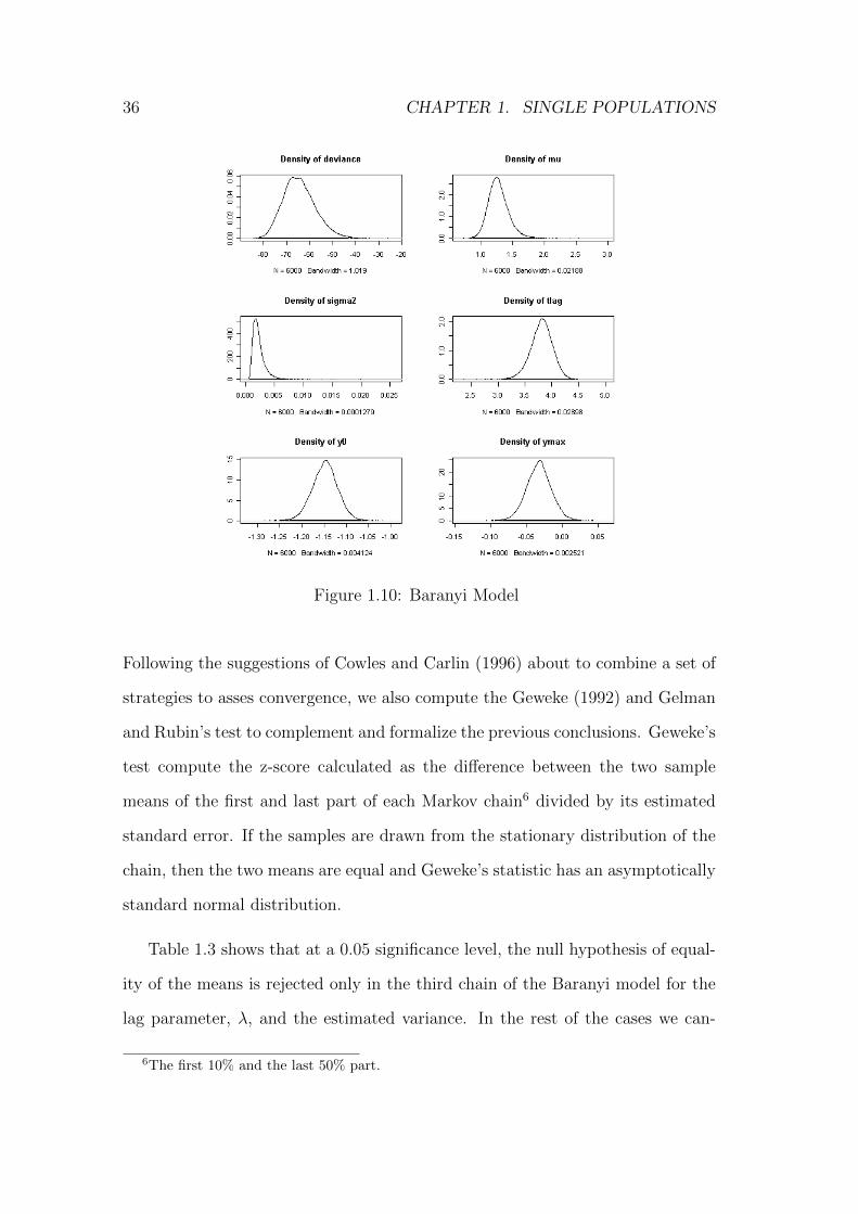
Figure 1.10: Baranyi Model
Following the suggestions of Cowles and Carlin (1996) about to combine a set of
strategies to asses convergence, we also compute the Geweke (1992) and Gelman
and Rubin’s test to complement and formalize the previous conclusions. Geweke’s
test compute the z-score calculated as the difference between the two sample
means of the first and last part of each Markov chain6 divided by its estimated
standard error. If the samples are drawn from the stationary distribution of the
chain, then the two means are equal and Geweke’s statistic has an asymptotically
standard normal distribution.
Table 1.3 shows that at a 0.05 significance level, the null hypothesis of equal-
ity of the means is rejected only in the third chain of the Baranyi model for the
lag parameter, λ, and the estimated variance. In the rest of the cases we can-
6The first 10% and the last 50% part.

1.6. APPLICATION: LISTERIA MONOCYTONGENES 37
Table 1.3: Geweke’s test
lag mu N0 Nmax sigma2Baranyi model:Chain 1 -0.494 -0.401 -0.794 1.180 -1.567Chain 2 0.052 0.115 -1.150 0.610 -1.857Chain 3 2.225 1.743 0.916 -0.588 1.973Gompertz model:Chain 1 0.519 -0.500 -0.077 -1.862 -1.494Chain 2 -0.647 -0.918 -0.072 0.236 0.318Chain 3 0.387 0.363 0.128 0.226 -1.879
not reject the null hypothesis, which indicates convergence of the Markov chain.
Convergence is also supported by the Gelman and Rubin test. For almost all
the parameters in both models, the scalar factor is equal to one, which indicates
convergence (only for the case of the maximum specific growth rate, µmax, in the
Gompertz model, the scalar factor is different to one and is equal to 1.27, which
is not too far from one).
Table 1.4: Descriptive statistics of Bayesian inference
Mean Median Std. Error 2.50% 97.50%Baranyi’s model:λ 3.807 3.816 0.207 3.370 4.193µmax 1.272 1.258 0.162 0.996 0.005N0 -1.149 -1.148 0.029 -1.211 -1.091Nmax -0.033 -0.033 0.018 -0.068 0.002σ2 0.002 0.002 0.001 0.001 0.005
Gompertz’s model:λ 3.098 3.102 0.232 2.630 3.538µmax 0.765 0.754 0.180 0.620 0.951N0 -1.127 -1.126 0.027 -1.182 -1.074Nmax -0.022 -0.022 0.019 -0.059 0.016σ2 0.002 0.002 0.001 0.001 0.005
The empirical posterior distributions of the model parameters are represented
in Figure 1.10 for the Baranyi model and in Figure 1.11 for the Gompertz model.
Several descriptive statistics are shown in Table 1.4. In both models, posterior
distributions of the parameters are reasonably symmetric except for σ2 that is
slightly skewed to the right. Posterior means of the parameters are relatively

38 CHAPTER 1. SINGLE POPULATIONS
close to the least squares estimates. As in the least squares method, the greater
difference between the two models is found in the lag parameter. The estimated
standard error is always greater in Bayesian inference than in the case of least
square method. Table 1.4 also shows the estimated high posterior density inter-
vals. Note that in Bayesian inference we deals with credible intervals which are
different from the classical concept of confidence intervals.
Figure 1.11: Gompertz Model
1.7 Conclusions
In this chapter, we have presented a brief description of the main population
growth models, focusing in the advantages and disadvantages of each one. Then

1.7. CONCLUSIONS 39
we have shown that given a single sample of data from one of these models, it is
straightforward to implement both classical and Bayesian inference for these mod-
els. In the following chapter, we shall consider how to extend the basic approach
outlined here to the case when various replications of a Petri dish experiment are
carried out under identical conditions and we would expect that the information
learned from one set of growth curve data is relevant to the prediction of a new
growth curve, motivating the use of hierarchical models.

40 CHAPTER 1. SINGLE POPULATIONS

Chapter 2
Hierarchical models for multiple
populations
One of the main characteristics of microbiological experiments is that typically,
researchers can replicate the same experiment several times under equal condi-
tions. For example, in Petri dish experiments, bacteria are collected and grown in
Petri dishes prepared with certain levels of nutrients and it is possible to repeat
the same experiment under similar conditions many times. However, up to now,
there has been little research on incorporating multiple experimental results into
the prediction of bacterial growth under fixed conditions. In this chapter, we
shall examine the situation when we observe the growth of r > 1 bacteria popu-
lations under identical environmental conditions and we shall develop a Bayesian,
hierarchical modeling approach for systems of this type.
41

42 CHAPTER 2. HIERARCHICAL MODELS
2.1 Introduction
Growth or longitudinal data consist of repeated observations of a growth process
or of a given characteristic over time among a population of individuals. For
instance, in medicine, height and weight may be measured for children at con-
secutive ages to control their development. Other examples are measurements of
blood pressure, cholesterol or tumour volume at different moments of time for
different patients. In ecology, the mean size of fin fish or shellfish, for instance,
are measured at different ages; in biology, animal populations are measured over
time, etc. Finally, in microbiological experiments, bacterial growth is observed
over time for several experiments undertaken under equal environmental condi-
tions.
In contrast to generalized linear models where the response variable can be
assumed to be independent, in the presence of this kind of data, with repeated
measurements for each subject, independence is unlikely. These dependencies
must be taken into account to correctly model the underlying processes and to
this end, various statistical procedures might be considered.
To illustrate in a simple way the different approaches that can be followed,
consider the case that repeated measures of a continuous response variable are
observed over time for each of m subjects. Let yij be the measurement of the
characteristic observed of individual i at time tij, for i = 1, . . . ,m and j =
1, . . . , ni and ni be the total number of observations of individual i. For this data
we consider three kinds of model.
The first approach assumes a common or pooled mean effect, µ. Assuming a

2.1. INTRODUCTION 43
normal distribution the model can be expressed as:
Yij|µ, σ ∼ N (µ, σ2) for i = 1, . . . ,m and j = 1, . . . , ni. (2.1)
Under this model, all observations are assumed to come from a common distri-
bution. However, the assumption that the mean and variance are the same for
all individuals may be unrealistic in cases where the population is heterogeneous
for example.
A second approach assumes different, independent mean effects, µi, for each
individual i. The model is:
Yij|µi, σ ∼ N (µi, σ2) for i = 1, . . . ,m and j = 1, . . . , ni. (2.2)
This model estimates the expected performance of each individual. However,
each mean effect is independent of the other individuals which does not seem
a realistic assumption when the behaviour of one individual is expected to be
similar to that of the others.
Finally, a third approach assumes that each mean effect µi is a sample from a
common population distribution with mean µ, called the population mean effect.
A new level of hierarchy is added to the model of (2.2) to give:
µi|µ,w ∼ N (µ,w2). (2.3)
In this model, the random effects, µi, are related and we can learn something
about one individual observing the others. Therefore, it is possible to obtain
more accurate estimations due to borrowing strength among individuals and this
effect is specially important when we deal with few number of observations for

44 CHAPTER 2. HIERARCHICAL MODELS
some of the subjects.
Note also that models with further levels of hierarchy could easily be consid-
ered. For example where the mean effect, say µit, is dependent on time and then
we might assume that the mean of µit, say µi, just depends on the individual i,
and finally that the individual effects µi are distributed around some common
mean µ.
2.1.1 Bayesian Hierarchical Modeling
Various approaches to inference for random effects or longitudinal models can be
considered. Firstly, classical methods are well reviewed in e.g. Fitzmaurice et al.
(2008). A second approach is to consider empirical Bayes methods whereby the
so called hyperparameters, µ,w of the distribution of µi in (2.3) are estimated
from the data via e.g. maximum likelihood or method of moments techniques
and then the analysis proceeds in a Bayesian way. See e.g. Cassella (1985) for a
good introduction to this approach.
In contrast to the empirical Bayes approach, fully hierarchical Bayesian anal-
yses can be carried out by specifying hyperprior distributions for these hyperpa-
rameters.
In our example, the model of (2.2) and (2.3) is completed by adding a hyper-
prior distribution for the hyperparameters, µ,w. For example,
µ|w ∼ N(
0,w2
c
)1
w2∼ G(a, b). (2.4)
Given these prior distributions, inference for the parameters of interest, e.g. µi, σ2

2.2. A HIERARCHICAL GOMPERTZMODEL FOR BACTERIAL GROWTH45
can be carried out by simply integrating out the hyperparameters, for example
p(µ1, . . . , µm, σ2|y) ∝ p(y|µ1, . . . , µm, σ
2)
∫ ∫p(µ1, . . . , µm|µ,w)p(µ,w) dµ dw.
(2.5)
As is typical in hierarchical models, the distribution in (2.5) does not have
a simple form. However, it is easy to see that the conditional distributions,
p(µ|y, . . . , µm, w), p(w|y, µ1 . . . , µm, µ) and p(µ1, . . . , µm|y, µ, w) can all be eas-
ily evaluated which implies that inference can be carried out using e.g. a Gibbs
sampling type algorithm. Algorithms of this type are now the standard tool for
the practical analysis of Bayesian hierarchical models. For a good recent review
of Bayesian hierarchical modeling, see e.g. Congdon (2010).
2.2 A hierarchical Gompertz model for bacte-
rial growth
As was presented in the previous chapter, the modified Gompertz equation is a
well known model for bacterial growth over time. This model has a sigmoidal
shape which reflects the three stages that characterize the bacterial growth pro-
cess: the lag stage, the exponential stage and the stationary stage. If Nt repre-
sents the population size of bacteria cultivated in a Petri dish experiment at time
t ≥ 0, then the modified Gompertz model can be expressed as
E[Nt|N0, D, µ, λ] = N0 +D exp
(− exp
(1 +
µe(λ− t)D
))≡ g(t, N0, D, µ, λ) say. (2.6)

46 CHAPTER 2. HIERARCHICAL MODELS
where e is the Euler’s number, N0 is the initial bacterial density, D is the max-
imum possible growth and is equal to the difference between the maximum bac-
terial density and the initial population density, µ is the maximum growth rate
and λ is the time lag.
Now, assume that r bacterial growth experiments under fixed conditions were
measured over time. Let Nij be the population density of replication i at time
tij, where i = 1, . . . , r, j = 0, . . . , ni and ni is the total number of observations of
replication i.
As was explained previously in Section 2.1, one possible approach to model
this kind of process is to assume that the growth curve has the same nature
for every experiment or replica. We can represent this by assuming a common
model for each growth curve. We call this a pooled model and express this in the
following form:
E[Nij|N0, D, µ, λ] = g(t,D,N0, µ, λ). (2.7)
Often it is not possible to fully control all the circumstances under which the
experiment of bacteria are carried out and could be appreciable variation among
different Petri dishes. Therefore, a disadvantage of this approach is that it does
not take into account any specific, unobserved, characteristics of the growth pro-
cess. A second possibility is to estimate each growth curve independently, follow-
ing the approach of Section 1.6.1, but this does not take into account the fact that
we should expect the different subjects to grow in a similar way under the same
conditions. Therefore we propose a a hierarchical modeling approach. Under this
approach each population follows its own growth process that is characterized by
its own growth parameters but these parameters are considered as a sample from

2.2. A HIERARCHICAL GOMPERTZMODEL FOR BACTERIAL GROWTH47
a common distribution.
Hence, we extend (2.6) to the case of hierarchical Gompertz model. This can
be expressed as
E[Nij|Ni0, Di, µi, λi] = Ni0 +Di exp
(− exp
(1 +
µie(λi − tij)Di
))≡ g(tij, Ni0, Di, µi, λi). (2.8)
Here, instead of a sampling process that comes from a unique density function,
now the growth data of each experiment is produced by a distinct but related
mechanism because of the common population density. In other words, each
particular experiment grows according to its own Gompertz curve with growth
parameters drawn from the common population density. This is a hierarchical
model structure as described in the previous section.
In order to complete the basic model, we shall assume that the observations
can be expressed as
Nij = g(tij, Ni0, Di, µi, λi) + εtij.
and will define a normal distribution for the errors.
One possiblility would be to consider independent, identically distributed er-
rors. However, Figure 2.1 illustrates different bacterial growth curves from petri
dish experiments under the same conditions (T=42, pH=7.4 and NaCI=2.5%).
It can be seen that the curves are closer together initially when the population
density is lower and then diverge over time as the population density grows which
suggests that the error variance should increase with population density.

48 CHAPTER 2. HIERARCHICAL MODELS
5 10 15
0.0
02
0.4
0.6
08
1.0
1.2
Hours
Pop
ulat
ion
size
5 10 15
0.0
02
0.4
0.6
08
1.0
1.2
Hours
Pop
ulat
ion
size
5 10 15
0.0
02
0.4
0.6
08
1.0
1.2
Hours
Pop
ulat
ion
size
5 10 15
0.0
02
0.4
0.6
08
1.0
1.2
Hours
Pop
ulat
ion
size
5 10 15
0.0
02
0.4
0.6
08
1.0
1.2
Hours
Pop
ulat
ion
size
5 10 15
0.0
02
0.4
0.6
08
1.0
1.2
Hours
Pop
ulat
ion
size
5 10 15
0.0
02
0.4
0.6
08
1.0
1.2
Hours
Pop
ulat
ion
size
5 10 15
0.0
02
0.4
0.6
08
1.0
1.2
Hours
Pop
ulat
ion
size
5 10 15
0.0
02
0.4
0.6
08
1.0
1.2
Hours
Pop
ulat
ion
size
5 10 15
0.0
02
0.4
0.6
08
1.0
1.2
Hours
Pop
ulat
ion
size
5 10 15
0.0
02
0.4
0.6
08
1.0
1.2
Hours
Pop
ulat
ion
size
5 10 15
0.0
02
0.4
0.6
08
1.0
1.2
Hours
Pop
ulat
ion
size
5 10 15
0.0
02
0.4
0.6
08
1.0
1.2
Hours
Pop
ulat
ion
size
5 10 15
0.0
02
0.4
0.6
08
1.0
1.2
Hours
Pop
ulat
ion
size
5 10 15
0.0
02
0.4
0.6
08
1.0
1.2
Hours
Pop
ulat
ion
size
5 10 15
0.0
02
0.4
0.6
08
1.0
1.2
Hours
Pop
ulat
ion
size
5 10 15
0.0
02
0.4
0.6
08
1.0
1.2
Hours
Pop
ulat
ion
size
5 10 15
0.0
02
0.4
0.6
08
1.0
1.2
Hours
Pop
ulat
ion
size
5 10 15
0.0
02
0.4
0.6
08
1.0
1.2
Hours
Pop
ulat
ion
size
5 10 15
0.0
02
0.4
0.6
08
1.0
1.2
Hours
Pop
ulat
ion
size
Figure 2.1: Growth curves under fixed environmental conditions: T=42, pH=7.4and NaCI=2.5%
Therefore, we shall assume the following model:
εtij|g(tij), σ, p ∼ N(0, σ2g(tij)
p)
(2.9)
where g(.) is the Gompertz function, σ2 ≥ 0 and p ≥ 0.5 so that the possibility
that the error variance increases with the population size is allowed for.
2.3 Bayesian inference
In order to fit the hierarchical model described in the previous section, one pos-
sibility would be to use classical, random effects techniques, but here, we prefer
to use a fully Bayesian approach. In microbiology risk assessment is important
to distinguish two sources of risk, variability and uncertainty. Uncertainty is de-
fined as the lack of perfect knowledge of some particular value. It may be reduced
by additional measurements. Variability represents the true heterogeneity of a
population and it can not be reduced by further information or studies. The

2.3. BAYESIAN INFERENCE 49
bacterial growth process is intrinsically variable: the growth curve observed in a
Petri dish may not be equal as that of another experiment even when all growth
conditions are the same. The growth process is also uncertain mainly due to that
the microbial measurements are imperfect. In a Bayesian approach variability
and uncertainty for the growth parameters can be modelled by means of a hi-
erarchical structure and the hyperparameters. Moreover, the Bayesian approach
makes it possible to incorporate various sources of previous information such as
expert knowledge, or previous empirical results which are typically plentiful in
the field of microbiology.
In order to implement Bayesian inference, we must also define distributions
for the unknown growth parameters and the hyperparameters. Firstly, we assume
the following priors for the growth parameters:
Nij|Ni0, Di, µi, λi, σ ∼ N(g(tij, Ni0, Di, µi, λi), σ
2)
Ni0|m0, s0 ∼ N(m0, s
20
)logDi|αD, τD ∼ N
(αN , τ
2N
)log µi|αµ, τµ ∼ N
(αµ, τ
2µ
)log λi|αλ, τλ ∼ N
(αλ, τ
2λ
)where σ2 is an unknown variance assumed to be common for each growth curve
and αD, τD, m0, s0, αµ, τµ, αλ, τλ are unknown hyperparameters. We will typi-
cally have very good prior knowledge concerning the initial population densities
Ni0, as the Petri dishes are typically seeded to some theoretical level.
Secondly, we consider an inverse gamma distribution for the model variance
σ2, that is
1
σ2∼ G (a, b) .

50 CHAPTER 2. HIERARCHICAL MODELS
Small values can be fixed for the parameters a, b to reflect an absence of prior
information.
Finally, the prior specification is completed by setting vague, but proper prior
distributions for the remaining hyperparameters:
αD ∼ N (mD, sD)1
τ 2D
∼ G (rD, vD)
αλ ∼ N (mλ, sλ)1
τ 2λ
∼ G (rλ, vλ)
αµ ∼ N (mµ, sµ)1
τ 2µ
∼ G (rµ, vµ)
where mD, mλ, mµ, sD, sλ, sµ, rD, rλ, rµ, vD, vλ and vµ are assumed known and
fixed.
Given the observed data, the likelihood function can be easily derived from
(2.9) as:
f(Nij|Ni0, Di, µi, λi, σ2) =
r∏i=1
n∏j=1
1√2πσ2
exp
(−(Nij − g(tij))
2
2σ2
)
∝ exp
(− 1
2σ2
r∑i=1
n∑t=1
(Nit − g(tij))2
)
where g(tij) is the modified Gompertz equation.
Unfortunately, given the nonlinearity of this model, the joint posterior param-
eter distribution does not have a simple form and, even the conditional posterior
distributions of most of the growth parameters cannot be obtained in a simple
closed form. Therefore, Markov-Chain Monte-Carlo (MCMC) techniques must
be employed to allow us to generate an approximate Monte Carlo sample from
the posterior parameter distributions. As in the previous Chapter, we propose to

2.3. BAYESIAN INFERENCE 51
use WinBUGS to implement the MCMC sampler. In this case, implementation is
carried out in using WinBUGS in combination with R, via the R2WinBUGS package
available from
http://cran.r-project.org/web/packages/R2WinBUGS/.
In a similar way to Figure 1.6 in the previous chapter, Figure 2.2 illustrates
the dependence structure of the model in WinBUGS style. WinBUGS code can be
constructed based on the doodle.
Figure 2.2: Doodle showing the dependence structure of the hierarchical Gom-pertz model
As WinBUGS is a generic approach to MCMC sampling, it is important to check
on the convergence of the sampler. Various tools can be used to check the conver-
gence. In particular, as well as standard graphical techniques such as looking at
the trace, the evolution of the mean and the autocorrelations of the sampled out-
put, we also use formal diagnostic techniques such as the modified Gelman-Rubin
statistic, discussed in the previous chapter.

52 CHAPTER 2. HIERARCHICAL MODELS
For the pooled and the independent models we follow the same approach as
before, assuming relatively uninformative log-normal prior distributions for the
non-negative Gompertz parameters D, λ and µ, and a vague inverse-gamma prior
distribution for σ2. Inference for these models is also implemented via WinBUGS.
2.4 Application: Listeria monocytogenes
In our application the models are fitted to listeria growth curves. Data come
from an experiment in broth monoculture where bacteria growth curves were
generated at fixed temperature, (42 ), acidity (pH = 7.4) and salt concentration
(2, 5% NaCl) levels and measured as optical density. Observations were equally
spaced and measurement times were common across replications. The data set
consists of 20 curves, each observed at 16 fixed time intervals of one hour are
those that we have seen previously in Figure 2.1.
We assume that bacteria grows according to the Gompertz equation of (2.6)
and compare the hierarchical, independent and pooled models described earlier
in Section 2.2. In order to fit the models, in each case we generated two parallel
chains using different initial values with 350000 iterations each, including 250000
iterations of burn-in. To diminish the autocorrelation between the generated val-
ues we also used a thinning rate of 10. Trace plots and autocorrelation functions
were used to check convergence and in all cases it was found that the burn-in pe-
riod was reasonable. Furthermore, the Gelman-Rubin statistic was equal o very
close to 1, giving a good indicator of convergence.

2.4. APPLICATION: LISTERIA MONOCYTOGENES 53
Table 2.1: Posterior mean parameter estimates and standard deviations in theindependent model
Replicate N0 sd D sd µ sd λ sd1 0.07 0.04 0.91 0.10 0.25 0.09 4.98 0.692 0.07 0.04 0.95 0.09 0.26 0.09 4.74 0.653 0.08 0.04 0.92 0.09 0.25 0.09 4.88 0.674 0.07 0.04 0.86 0.09 0.25 0.10 4.87 0.735 0.07 0.04 0.93 0.10 0.24 0.09 4.87 0.696 0.07 0.04 0.86 0.09 0.25 0.10 4.88 0.717 0.07 0.04 0.87 0.09 0.24 0.09 4.80 0.718 0.07 0.04 0.87 0.09 0.24 0.09 4.86 0.729 0.08 0.04 0.92 0.10 0.24 0.08 4.84 0.6910 0.07 0.04 1.00 0.10 0.26 0.08 4.93 0.6311 0.07 0.04 0.91 0.10 0.25 0.09 4.93 0.7012 0.07 0.04 0.86 0.10 0.23 0.08 4.82 0.7613 0.07 0.04 0.82 0.10 0.23 0.09 4.88 0.8014 0.07 0.04 0.84 0.10 0.23 0.09 4.89 0.7715 0.07 0.04 0.82 0.10 0.23 0.10 4.87 0.8016 0.07 0.04 0.86 0.10 0.24 0.10 4.95 0.7517 0.07 0.04 0.86 0.10 0.23 0.09 4.90 0.7518 0.07 0.04 0.93 0.09 0.26 0.09 4.92 0.6519 0.07 0.04 0.85 0.09 0.25 0.10 4.91 0.7220 0.07 0.04 0.89 0.10 0.23 0.08 4.80 0.71
Mean 0.89 0.24 4.88
Independent model
Table 2.1 summarizes the estimated growth parameters for the independent model.
The posterior mean and the standard deviation for each parameter are shown.
Comparing the values of the estimated parameters for each curve, we can see the
range of variation which indicates that there are significant differences among
curves even when the environmental conditions are the same for all the cases.
The maximum specific growth rate ranges from 0.23 to 0.26, the lag parameter
ranges from 4.74 to 4.98 and the maximum population size ranges from 0.82 to
1.00. The differences between the initial population size are very small, while the
maximum observed differences are observed in the maximum population size.
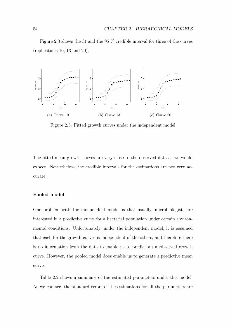
54 CHAPTER 2. HIERARCHICAL MODELS
Figure 2.3 shows the fit and the 95 % credible interval for three of the curves
(replications 10, 13 and 20).
0 5 10 15
0.0
0.5
1.0
Hour
Pop
ulat
ion
size
0 5 10 15
0.0
0.5
1.0
0 5 10 15
0.0
0.5
1.0
0 5 10 15
0.0
0.5
1.0
(a) Curve 10
0 5 10 15
0.0
0.5
1.0
Hour
Pop
ulat
ion
size
0 5 10 15
0.0
0.5
1.0
0 5 10 15
0.0
0.5
1.0
0 5 10 15
0.0
0.5
1.0
(b) Curve 13
0 5 10 15
0.0
0.5
1.0
Hour
Pop
ulat
ion
size
0 5 10 15
0.0
0.5
1.0
0 5 10 15
0.0
0.5
1.0
0 5 10 15
0.0
0.5
1.0
(c) Curve 20
Figure 2.3: Fitted growth curves under the independent model
The fitted mean growth curves are very close to the observed data as we would
expect. Nevertheless, the credible intervals for the estimations are not very ac-
curate.
Pooled model
One problem with the independent model is that usually, microbiologists are
interested in a predictive curve for a bacterial population under certain environ-
mental conditions. Unfortunately, under the independent model, it is assumed
that each for the growth curves is independent of the others, and therefore there
is no information from the data to enable us to predict an unobserved growth
curve. However, the pooled model does enable us to generate a predictive mean
curve.
Table 2.2 shows a summary of the estimated parameters under this model.
As we can see, the standard errors of the estimations for all the parameters are

2.4. APPLICATION: LISTERIA MONOCYTOGENES 55
lower with the pooled model compared with the independent one. The reason
is that to estimate this growth parameters we use the information from all of
the replications in the group because each observed growth curve is assumed to
be a sample from a unique growth curve implying that we have a larger sample
and therefore reduced uncertainty, leading to increased precision when estimating
the unknown parameters. The estimated curve can be interpreted as the mean
bacterial growth curve under given environmental conditions.
Table 2.2: Posterior mean parameter estimates and standard deviations in thepooled model
N0 D µ λmean 0.08 0.87 0.23 5.00
sd 0.00 0.01 0.01 0.04
Figure 2.4 shows the fit of the pooled model. The solid line represents the
posterior mean and the dashed lines are the 95% credible intervals. Dotted lines
are 3 of the replications, curve 10, curve 13 and curve 20. Some observations
from curve 10 fall outside of the credible interval. As expected, the posterior
mean curve can be seen as the mean of the observed curves, but fails to describe
the exact behaviour of each individual curve.
Hierarchical model
The summary of the estimated parameters with the hierarchical model are pre-
sented in Table 2.3. The posterior mean and standard deviation of the estimated
parameters of each curve are shown and also for the population parameters. The
estimated parameter values for each curve are very similar to those obtained

56 CHAPTER 2. HIERARCHICAL MODELS
0 5 10 15
0.0
02
0.4
0.6
08
1.0
1.2
Hours
Pop
ulat
ion
size
0 5 10 15
0.0
02
0.4
0.6
08
1.0
1.2
Hours
Pop
ulat
ion
size
0 5 10 15
0.0
02
0.4
0.6
08
1.0
1.2
Hours
Pop
ulat
ion
size
0 5 10 15
0.0
02
0.4
0.6
08
1.0
1.2
0 5 10 15
0.0
02
0.4
0.6
08
1.0
1.2
0 5 10 15
0.0
02
0.4
0.6
08
1.0
1.2
Figure 2.4: Fit of the Pooled model
with the independent model. However, the standard errors are significantly lower
for the hierarchical model. To summarize the behaviour of the bacterial growth
with the given environmental growth we can use the estimated population growth
parameters.
0 5 10 15
0.0
0.5
1.0
Hour
Pop
ulat
ion
size
0 5 10 15
0.0
0.5
1.0
0 5 10 15
0.0
0.5
1.0
0 5 10 15
0.0
0.5
1.0
(a) Curve 10
0 5 10 15
0.0
0.5
1.0
Hour
Pop
ulat
ion
size
0 5 10 15
0.0
0.5
1.0
0 5 10 15
0.0
0.5
1.0
0 5 10 15
0.0
0.5
1.0
(b) Curve 13
0 5 10 15
0.0
0.5
1.0
Hour
Pop
ulat
ion
size
0 5 10 15
0.0
0.5
1.0
0 5 10 15
0.0
0.5
1.0
0 5 10 15
0.0
0.5
1.0
(c) Curve 20
Figure 2.5: Fitted Growth curves under the hierarchical model
To compare the parameter estimations of the different models, the main re-
sults for the parameters modeled with hierarchical structure are included in Table

2.4. APPLICATION: LISTERIA MONOCYTOGENES 57
Table 2.3: Posterior mean parameter estimates and standard deviations in thehierarchical model
Replicate N0 sd D sd µ sd λ sd1 0.08 0.01 0.90 0.02 0.24 0.02 5.08 0.142 0.08 0.01 0.94 0.02 0.25 0.02 4.83 0.145 0.08 0.01 0.92 0.02 0.23 0.02 4.97 0.156 0.08 0.01 0.85 0.02 0.24 0.02 4.99 0.147 0.08 0.01 0.86 0.02 0.23 0.02 4.92 0.158 0.08 0.01 0.86 0.02 0.23 0.02 4.98 0.159 0.08 0.01 0.91 0.02 0.23 0.02 4.95 0.1510 0.08 0.01 0.99 0.02 0.25 0.02 5.01 0.1411 0.08 0.01 0.89 0.02 0.24 0.02 5.05 0.1412 0.08 0.01 0.85 0.02 0.22 0.02 4.97 0.1513 0.08 0.01 0.81 0.02 0.22 0.02 5.03 0.1614 0.08 0.01 0.82 0.02 0.22 0.02 5.04 0.1615 0.08 0.01 0.80 0.02 0.22 0.02 5.03 0.1616 0.08 0.01 0.85 0.02 0.23 0.02 5.07 0.1517 0.08 0.01 0.84 0.02 0.22 0.02 5.05 0.1518 0.08 0.01 0.92 0.02 0.24 0.02 4.99 0.1419 0.08 0.01 0.84 0.02 0.24 0.02 5.03 0.1520 0.08 0.01 0.88 0.02 0.23 0.02 4.93 0.15
Population mean (αi) 0.92 0.07 0.25 0.02 5.23 0.39Population sd (τi) 0.32 0.05 0.09 0.00 1.78 1.48
2.4. The posterior mean and the 95% credible interval for the population growth
parameters are shown for the full hierarchical model, the mixed model and the
pooled model. Moreover, for the first two models and for the independent one,
individual parameters are shown for curves 10, 13 and 20 - the same curves rep-
resented graphically before. When comparing among the individual parameter
estimations between the independent model and the hierarchical models, it can be
seen that there are small differences. However, if we look at the credible intervals
it is possible to see that in hierarchical models the estimations are more precise.
Regarding the population parameters, we observe some differences between the
estimated parameters values between the pooled model and the hierarchical mod-
els. But, the credible intervals of the hierarchical models include the estimated

58 CHAPTER 2. HIERARCHICAL MODELS
Table 2.4: Parameter estimations
D Mu Lambdamean 95% mean 95% mean 95%
Independent modelCurve 10 1.00 (0.83 1.22) 0.26 (0.14 0.50) 4.93 (3.53 6.10)Curve 13 0.82 (0.66 1.05) 0.23 (0.10 0.49) 4.88 (2.97 6.27)Curve 20 0.89 (0.73 1.12) 0.23 (0.11 0.47) 4.80 (3.15 6.08)
Hierarchical modelCurva 10 0.99 (0.95 1.03) 0.25 (0.22 0.28) 5.01 (4.74 5.28)Curva 13 0.81 (0.77 0.84) 0.22 (0.18 0.26) 5.03 (4.70 5.35)Curva 20 0.88 (0.84 0.91) 0.23 (0.19 0.26) 4.93 (4.63 5.22)Population 0.92 (0.80 1.08) 0.25 (0.21 0.29) 5.23 (4.53 6.08)
Pooled modelPopulation 0.87 (0.86 0.88) 0.23 (0.22 0.24) 5.00 (4.90 5.08)
values with the former model.
Prediction
To asses the predictive capacity of the models, we consider two types of predic-
tions: one and various step ahead predictions for a given curve, and the prediction
of a new curve. Firstly, consider the case where the first 19 curves are fully ob-
served and where only the first 6 values of the 20th curve are observed, so that
we can try to predict the trajectory of the rest of the growth curve. Figure 2.6
shows the predictive curves for the hierarchical and pooled models respectively.
The predictive curve for the hierarchical model is more accurate than the one
for the pooled model. Moreover, when computing the mean squared error be-
tween the predictive curve and the real curve, the value for the former model is
equal to 0.0020 while for the later is equal to 0.0042. In general, the more the
growth process differs from the mean, the better the hierarchical model performs
in comparison with the pooled model.

2.4. APPLICATION: LISTERIA MONOCYTOGENES 59
Now, we will consider the case of prediction for a new curve, J which at
the beginning has not been observed at all. The procedure is as follows. First,
having observed the previous 19 curves, we will predict the cell density of the
new curve at t = 0. Then, given the true value of the bacteria density at that
time, we predict the following value, that is the cell density at t = 1. After that,
we observed the first two points and predictive the population density at t = 3
and so on. Figure 2.7 shows the predictive curves for a new experiment for the
hierarchical model and the pooled model, respectively.
5 10 15
0.0
0.5
1.0
1.5
Curve 18
N
5 10 15
0.0
0.5
1.0
1.5
5 10 15
0.0
0.5
1.0
1.5
5 10 15
0.0
0.5
1.0
1.5
(a) Hierarchical model
5 10 15
0.0
0.2
0.4
0.6
0.8
1.0
1.2
Curve 18
N
5 10 15
0.0
0.2
0.4
0.6
0.8
1.0
1.2
5 10 15
0.0
0.2
0.4
0.6
0.8
1.0
1.2
5 10 15
0.0
0.2
0.4
0.6
0.8
1.0
1.2
(b) Pooled model
Figure 2.6: The predictive mean curve for future observations
Once again, the hierarchical model outperforms the pooled model with the
predicted curve being very close to the true curve. The mean square error of the
predictions are equal to 0.0006 and 0.0040, for the hierarchical and the pooled
model respectively, being significantly lower for the hierarchical model.
Finally, if we want to answer the previously mentioned questions of the mi-
crobiologists with the models presented here we have two possibilities. The first
one is to use the posterior predictive distribution of the pooled model. The mean
curve was represented in Figure 2.4. The second possibility is to use the hierarchi-
cal model: with the posterior distribution of the population parameters (learned
from the observed curves) in combination with the prior distribution of the in-

60 CHAPTER 2. HIERARCHICAL MODELS
5 10 15
0.0
0.2
0.4
0.6
0.8
1.0
1.2
Curve 18
N
5 10 15
0.0
0.2
0.4
0.6
0.8
1.0
1.2
(a) Hierarchical model
5 10 15
0.0
0.2
0.4
0.6
0.8
1.0
1.2
Curve 18
N
5 10 15
0.0
0.2
0.4
0.6
0.8
1.0
1.2
(b) Pooled model
Figure 2.7: Predictive Future Experiment
dividual parameters it is possible to derive a posterior predictive distribution for
the new curve. Calling θ the vector of individual growth parameters and φ the
vector of population parameters, the predictive distribution is equal to
p(ynew|yobs) =
∫θ
∫φp(ynew|θ)p(θ|φ)p(φ|yobs)dθdφ
A sample from that distribution can be easily obtained from the MCMC
previously generated.
Table 2.5: Predictive mean values at each time.
Hour 1 2 3 4 5 6 7 8HM 0.07 0.07 0.07 0.09 0.16 0.33 0.53 0.70PM 0.08 0.08 0.08 0.08 0.14 0.31 0.54 0.72
Hour 9 10 11 12 13 14 15 16HM 0.81 0.87 0.91 0.93 0.94 0.95 0.95 0.95PM 0.83 0.89 0.92 0.94 0.94 0.95 0.95 0.95
Figure 2.8 shows the predictive mean curve and the 95% credible interval.
Dotted points represent the various curves observed under the given fixed envi-

2.4. APPLICATION: LISTERIA MONOCYTOGENES 61
0 5 10 15
0.0
0.5
1.0
Hour
Pop
ulat
ion
size
0 5 10 15
0.0
0.5
1.0
Hour
Pop
ulat
ion
size
0 5 10 15
0.0
0.5
1.0
Hour
Pop
ulat
ion
size
0 5 10 15
0.0
0.5
1.0
Hour
Pop
ulat
ion
size
0 5 10 15
0.0
0.5
1.0
Hour
Pop
ulat
ion
size
0 5 10 15
0.0
0.5
1.0
Hour
Pop
ulat
ion
size
0 5 10 15
0.0
0.5
1.0
Hour
Pop
ulat
ion
size
0 5 10 15
0.0
0.5
1.0
Hour
Pop
ulat
ion
size
0 5 10 15
0.0
0.5
1.0
Hour
Pop
ulat
ion
size
0 5 10 15
0.0
0.5
1.0
Hour
Pop
ulat
ion
size
0 5 10 15
0.0
0.5
1.0
Hour
Pop
ulat
ion
size
0 5 10 15
0.0
0.5
1.0
Hour
Pop
ulat
ion
size
0 5 10 15
0.0
0.5
1.0
Hour
Pop
ulat
ion
size
0 5 10 15
0.0
0.5
1.0
Hour
Pop
ulat
ion
size
0 5 10 15
0.0
0.5
1.0
Hour
Pop
ulat
ion
size
0 5 10 15
0.0
0.5
1.0
Hour
Pop
ulat
ion
size
0 5 10 15
0.0
0.5
1.0
Hour
Pop
ulat
ion
size
0 5 10 15
0.0
0.5
1.0
Hour
Pop
ulat
ion
size
0 5 10 15
0.0
0.5
1.0
Hour
Pop
ulat
ion
size
0 5 10 15
0.0
0.5
1.0
Hour
Pop
ulat
ion
size
0 5 10 15
0.0
0.5
1.0
0 5 10 15
0.0
0.5
1.0
0 5 10 15
0.0
0.5
1.0
Figure 2.8: Predictive mean curve of a new replication
ronmental conditions. The estimated predictive curve is a good representation
of the mean behaviour of the bacterial growth process. The mean curve is very
similar to the mean curve of the pooled model (Table 2.5 shows the estimated
mean values of the curve for each time). Nevertheless, in contrast with the former
model, here all the curves lie inside the credible intervals. Finally, the posterior
mean of the growth parameters are very closed to those estimated with the pooled
model (see Table 2.6).
Table 2.6: Posterior mean of the growth parameters.
N0 Dmax µ λPooled 0.08 (0.00) 0.87 (0.01) 0.23 (0.01) 5.00 (0.04)
Hierarchical 0.07 (0.10) 0.88 (0.12) 0.24 (0.03) 4.99 (0.67)
The better performance of the hierarchical model with respect to the pooled
and the independent model regarding both, fitting and prediction, is also sup-
ported by the DIC and the MSE values. Table 2.4 shows that the hierarchical
model has a lower MSE indicating the goodness of fit but also a lower DIC which

62 CHAPTER 2. HIERARCHICAL MODELS
also penalizes for model complexity.
DIC MSEIM -646.23 1.98
HM -1489.62 0.02PM -1326.01 0.05
2.5 Conclusions
In this chapter, we have illustrated that hierarchical models can be used to model
bacterial growth functions when several replications of the same experiment un-
der equal environmental conditions such as temperature, acidity level and salt
concentration are available. Various simpler models, keeping some of the growth
parameters fixed, are also suitable.
A number of extensions to this approach are possible. Firstly, in this chapter
we have extended the modified Gompertz equation to the case of a hierarchical
model, but the approach is equally applicable to other bacterial growth models
such as the logistic or Baranyi models. Furthermore, it can also be applied to the
cases where we assume no parametric growth model and instead use a nonpara-
metric approach. Finally, in the present study we have considered experiments
under fixed environmental conditions. A natural extension of this work is to
consider modeling what happens at different levels of the environmental condi-
tions. These last two situations will be considered in the following chapters of
this thesis.

Chapter 3
Neural networks models
3.1 Introduction
In the previous chapter we have seen how to model and the predict the bacteria
growth process when environmental conditions are fixed. Nevertheless, in reality,
these external factors are not fixed. For instance, food products are affected
by different factors depending on environmental conditions in the production,
distribution, storage and consumption stage. Shelf life is determined by the
evolution and growth of the micro-organisms which can spoil the product and
cause pathogenic effects. The aim of predictive microbiology is to know which
environmental factors most influence the growth processes of micro-organisms
in food. The relationships between these factors are complex, interactive and
dynamic and therefore, it is important to develop secondary bacterial growth
models to predict the shelf life of perishable foods or the behaviour of food borne
pathogens.
In this chapter, we shall start by briefly summarizing the most popular sec-
ondary models and then propose two different approaches based on the use of
63

64 CHAPTER 3. NEURAL NETWORKS MODELS
neural network techniques. The first model is based on the Gompertz function
where the dependence of the growth parameters on the environmental factors is
modeled by a neural network. Secondly, we shall consider a direct, non-parametric
approach based on the use of neural networks as a primary growth model. An
important feature of our approaches is that in cases where we observe bacterial
growth in various colonies under possible different environmental conditions, we
use hierarchical modeling, as in Chapter 2, to improve the estimation of a single
growth curve by incorporating information from the various different bacterial
populations.
As in the previous chapter, inference for our models is undertaken throughout
using a Bayesian approach. One of the main problems with inference for neural
networks models was that typically, complicated inference algorithms need to be
designed and a great deal of tuning often needs to be carried out for these to
work efficiently, see e.g. Lee (2004). Here, however, we show that inference can
be still be carried out using WinBUGS.
3.2 Secondary models
Primary models for growth curve typically assume some parametric form, e.g. the
Gompertz curve for the growth model under specific environmental conditions.
It is natural however to suppose that growth will typically be different under
different environmental conditions and this can be done by allowing the model
parameters to vary depending on these conditions. Models for this variation in
parameters are called secondary models and some of the most important of these
are are outlined below.

3.2. SECONDARY MODELS 65
3.2.1 The square-root model
Ratkowsky et al. (1982) suggested a simple empirical model that describe the
effect of suboptimal temperature on growth rates of micro-organisms. Before
fitting the model to experimental growth rates, data is transformed taking the
square root in order to stabilize the variance and for this reason this model and
their future extensions are called square-root models. Suppose that µmax is the
maximum growth rate of a bacterium under optimal temperature conditions.
Then the basic square root model supposes that:
√µmax = b(T − Tmin) (3.1)
where b is a constant and Tmin is a parameter which indicates the minimum
temperature at which growth can occur. From growth curve observed at different
temperature levels, the parameters b and Tmin can be estimated by classical model
fitting techniques. This first equation was expanded to include the effect of other
factors besides temperatures, such as water activity, acidity level, salinity level,
etc. The extended version which describes the combined effect of temperature
and other factors can be expressed as
√µmax = b(T − Tmin)
√X −Xmin (3.2)
where b and Tmin are as previously defined, X is another factor different from T
such as water activity or level of acidity (pH) and Xmin is the minimum level of
the that factor below which growth is not possible. These models are simple, easy
to interpret and use few parameters. Each term expresses how an environmental
factor changes the growth rate of a micro-organism. However, as pointed out in
McKellar and Lu (2004), in these models, the expected multidimensional growth

66 CHAPTER 3. NEURAL NETWORKS MODELS
space is not influenced by the levels of the different environmental parameters.
Thus, for instance, the level of acidity influences the range of pH values for which
growth is theoretically observed.
3.2.2 Cardinal parameter models
Cardinal parameter models (CPMs) rely on the assumption that the inhibitory
effect of the environmental factors is multiplicative. This idea was formalized
in the gamma concept introduced in Zwietering et al. (1992). Under optimal
conditions a micro-organism has a maximum growth rate, but when any envi-
ronmental factor becomes suboptimal the growth rate declines and the extent
of that inhibition depends on the rate between the test condition compared to
that at the optimum. Thus, a CPM consists of a discrete term for each envi-
ronmental factor, where each term is the growth rate relative to that when that
factor is optimal. An extensive CPM developed for growth of Listeria monocy-
togenes, includes the effect of temperature (T ), water activity (aw), acidity level
(pH), inhibitory substances (ci), and qualitative factors (kj) on µmax and can be
expressed as:
µmax = µoptτ(T )ρ(aw)α(pH)I∏i=1
γ(ci)J∏j=1
kj (3.3)
where τ = CM2, ρ = CM1 and α = CM2 with
CMn=
0 if X ≤ Xmin
Xopt−Xmin)1−n(X−Xmax)(X−Xmin)n
([(Xopt−Xmin)(X−Xopt)−(Xopt−Xmax)((n−1)Xopt+Xmin−nX)]if Xmin < X < Xmax
0 X ≥ Xmax
γ(ci) =
(1− ci/MICi)2 if ci < MICi
0 otherwise

3.2. SECONDARY MODELS 67
where X is the temperature, water activity or pH, Xmin and Xmax are the values
of the factor X below and above which growth impossible, Xopt is the value at
which µmax is equal to its optimal value µopt and MICi the minimal inhibitory
concentration of specific compounds above which no growth occurs.
Cardinal models assume that different environmental factors have indepen-
dent and multiplicative effects on µmax. The assumption of independence might
not be reasonable in all cases. As is pointed out in McKellar and Lu (2004)
numerous studies have shown that the growth range of a micro-organism in one
environmental condition is affected by other environmental conditions.
3.2.3 Polynomial models
Polynomial models, also called response surface models, are probably the most
common secondary model. These kinds of models are relatively easy to fit by using
multiple linear regression techniques. Polynomial models are able to incorporate
different environmental factors and their interactive effects in a simple way. The
model can be expressed as:
θ = β0 +k∑j=1
βjXj +k∑j=1
βjjX2j +
∑j<l
k∑l=2
βjlXjXl (3.4)
where θ is the response variable, for instance a parameter of the primary growth
rate model, βj, βjj and βjl are the parameters of the model and the Xi are the
environmental factors such as temperature, salinity level, acidity level, etc. One
of the main criticisms of the polynomial models is that they have a high number
of parameters without biological interpretation that make difficult to compare
this kind of model with other secondary models.

68 CHAPTER 3. NEURAL NETWORKS MODELS
3.2.4 Artificial neural network models
Square-root models, cardinal parameter models and polynomial models all have
several versions depending on the micro-organisms, the environmental factors in-
cluded, the quantity of factors, the growth parameters which we want to explain
(growth rate, lag parameter, the maximum population size), etc. Due to the
long list of parametric models, it is possible to talk about model uncertainty.
Which model is the best? More recently artificial neural networks (ANNs) have
been proposed as a way to model complex non-linear systems (see e.g. Hajmeer
et al. (1997), Geeraerd et al. (1998) and Garcıa-Gimeno et al. (2002)). Neural
networks, in statistical terms, are non-parametric models, as opposed to the para-
metric models we have used earlier, which are characterized by a small number of
parameters, which often have a meaningful interpretation. Although neural net-
work models lose this easy interpretation, the advantages of neural networks are
their capability to describe very complex non-linear relationships and that they
do not impose any structure on the relationship between the interacting effects.
3.3 Neural network based growth curve models
In this section we give a brief presentation of artificial neural networks. We will
focus on feed forward neural networks, which are the most popular and widely
used network in many applications. Then we shall present two neural network
based models for bacteria growth, the first of which is a secondary model where
the parameters of the Gompertz curve are related to environmental factors using
ANNs and the second of which is a primary neural network model where no
specific form for the basic growth curve is presupposed.

3.3. NEURAL NETWORK BASED GROWTH CURVE MODELS 69
3.3.1 Feed forward neural networks
Assume that there are q dependent variables, (Y1, . . . , Yq) = Y, and a set of
explanatory variables, (x1, . . . , xp) = x. Often, the relationship between Y and
x is modeled by assuming a simple relationship such as e.g. multivariate regres-
sion. However, such a relationship may not always be appropriate and often, a
more general functional relation between the dependent and independent vari-
ables must be assumed, say
E[Y|x] = g(x)
where the functional form, (g1, . . . , gq) = g : Rp → Rq, is unknown.
One of the most popular methods of modeling the function g is via neural
networks, see e.g. Stern (1996). In particular, a feed forward neural network
takes a set of inputs x, and from them computes the vector of output values as
follows
g(x) = B ·ΨT (xTΓ) (3.5)
whereB is a q×M matrix with q ∈ N the number of output variables and M ∈ N
the number of nodes and Γ is a p ×M matrix with p ∈ N being the number of
explicative variables. The element γrk ∈ R is the weight of the connection from
input r to hidden unit k and the element βsk ∈ R is the weight connection from
hidden unit k to output unit s. Finally, Ψ(a1, . . . , aM) = (Ψ(a1), . . . ,Ψ(aM))
where Ψ is a sigmoidal function such as the logistic function
Ψ(x) =exp(x)
1 + exp(x), (3.6)
which we will use here. Equations (3.5) and (3.6) define a feed forward neural
network with a logistic activation function, p explanatory variables (inputs), one

70 CHAPTER 3. NEURAL NETWORKS MODELS
hidden layer with M nodes and q dependent variables (outputs) that is illustrated
in Figure 3.1. Note that each output in the neural network combines the node
values in a different way.
g1(x)
g2(x) Outputs. . .
gq(x)
1
2
3 M − 1
@@@
@@@I
. . . . . . M
x1
x2 . . .
xp
Hidden nodes
Inputs
6
@@@@@@I
HHHH
HHH
HHH
HHY
*
*
AAAAAAK
3
*
1
AAAAAAK
QQQ
QQQQk
HHHH
HHH
HHH
HHHY
PPPP
PPPP
PPPP
PPPP
PPPi
6
HHHH
HHH
HHH
HHY
QQQQQQQQQk
3
1
AAAAAAK
*
HHHH
HHH
HHH
HHHY
AAAAAAK
PPPP
PPPP
PPPP
PPPP
PPi
Figure 3.1: Neural network representation
Several features of neural networks make them valuable and attractive for pre-
dictive microbiology, where the environmental conditions that affect growth are
complex and poorly understood. First, ANNs have few prior assumptions about
the models for the problem studied. The network can learn from data and capture
subtle functional relationships even if the underlying relationships are unknown
or very complex to describe. Thus, ANNs are particularly useful when there is
little knowledge about the underlying laws governing the systems from which
data is generated but for which there are enough data or observations. ANNs
can also be used for prediction. After learning from data, an ANN can often give
good inferences about the unseen part of a population, such as prediction of the
future behaviour from knowing the past. Finally, ANNs are universal functional
approximators, meaning that a network can approximate any continuous function

3.3. NEURAL NETWORK BASED GROWTH CURVE MODELS 71
to any desired accuracy. ANNs have more general and flexible functional forms
which make possible to model very complex nonlinear systems. ANNs can deal
with nonlinear modeling without a priori assumptions about the relationships
between input and output variables.
Standard secondary growth curve models commented previously may not cap-
ture the complex relationships and interactions between growth and external fac-
tors such as temperature, pH or salt levels. Therefore, here we propose to use
neural networks to model the complex system of interactions between environ-
mental factors. In particular, we shall consider two neural network based models,
the first of which is a secondary model based on the Gompertz equation and the
second of which is a primary neural network model.
3.3.2 A neural network based Gompertz model
As we have commented previously, the Gompertz equation, has been used exten-
sively by researchers to fit a wide variety of growth curves from different microor-
ganisms. However, the primary growth model described in Equation (2.6) does
not allow for the case where we wish to study bacterial populations under a va-
riety of controlled environmental conditions. Therefore, suppose that we observe
the growth of I bacterial populations under similar initial conditions and that we
have J different environments determined by temperature, level of acidity (pH)
and salt concentration (NaCI). Now, because we want to know how the growth
process is affected by different external conditions, it may be reasonable to as-
sume that all replications have the same growth curve parameters under fixed
environmental conditions. However, growth rates will vary under different con-
ditions and therefore, assuming a Gompertz model, we propose the use of neural
networks to reflect the parameter dependence on the environmental factors. If

72 CHAPTER 3. NEURAL NETWORKS MODELS
Ntij is the concentration in population i under environmental conditions j at time
t the Gompertz function is
E[Ntij|N0j, Dj, µj, λj] = g(tij, N0j, Dj, µj, λj), (3.7)
where g(·) is as in (2.7), for i = 1, . . . , I and j = 1, . . . , J . Now, we model the
growth parameters µ, λ and D as a function of the temperature, the level of
acidity and the salt concentration by a feed forward neural network, that is
θs =M∑k=1
βsk ·Ψ(x′γk), for s = 1, 2, 3. (3.8)
where θs represents the parameters (D,µ, λ) and x = (T, pH,NaCI) is the vector
of explanatory variables representing the environmental conditions and Ψ is the
logistic function, so that
Ψ(x) =1
1 + exp(−x).
From now on, the model defined by (3.7) and (3.8) will be referred to as the GNN
model.
3.3.3 A hierarchical neural network model
Here, we generalize the previous model to a new one which does not assume any
underlying parametric growth function. Instead, we propose the use of a neural
network as a primary model. The output of the network is the instantaneous
reproduction rate per member of the population and the inputs are the current
population size and the experimental conditions. Formally, we can write this

3.3. NEURAL NETWORK BASED GROWTH CURVE MODELS 73
model as
E[Ntij|N(t−1)ij, fj, Tj, pHj, NaClj] =
N(t−1)ij +N(t−1)ijfj(N(t−1)ij, Tj, pHj, NaCIj) (3.9)
fj(N(t−1)ij, Tj, pHj, NaCIj) =M∑k=1
βjk(Ψ(γ1kN(t−1)ij + γ2kTj + γ3kpHj + γ4kNaCIj)
−Ψ(γ2kTj + γ3kpHj + γ4kNaCIj)), (3.10)
for i = 1, . . . , I and j = 1, . . . , J , fj(·) is the growth rate for populations with
environmental condition j. From now on, the model defined by (3.9) will be
referred to as the NN model.
3.3.4 Error modeling
In the previous subsections, two approaches to modeling the expected population
density have been provided. These models are completed by including an error
term. We might consider using independent, identically distributed errors, but,
in a similar way to (2.9) in the previous chapter it would appear more reasonable
to assume that the error variance increases with population size.
Therefore, in the case of the GNN model, we assume that the error term is
εtij|gtij, σ, p ∼ N(0, σ2g(tij)
p)
(3.11)
where g(.) is the Gompertz function as in (2.9).

74 CHAPTER 3. NEURAL NETWORKS MODELS
In the case of the NN model, we assume that
Ntij = N(t−1)ij +N(t−1)ijfj(N(t−1)ij, Tj, pHj, NaCIj) + εtij (3.12)
where we assume that the error term is
εtij|N(t−1)ij, σ, p ∼ N(0, σ2Np
t−1
). (3.13)
Note in particular that for p > 0, this error structure implies that if N(t−1)ij = 0,
then Ntij = 0, so that once the population has died out, then it remains extinct.
3.4 Bayesian inference for the neural network
models
Typically, when fitting secondary models using classical statistical procedures, a
two-stage procedure is carried out. In the first stage, a primary model is fitted to
the observed data in order to get the estimated growth parameter values under
each set of environmental conditions. The second stage then involves fitting a
secondary model to these using the sets of estimated parameters as data. These
two steps are usually not linked, which means that the uncertainty of the first
step is not taken into account in the second step. However, in a Bayesian context,
inference can be carried out directly using a one-step procedure.
Regarding fitting of neural networks, given a set of observed inputs and out-
puts, say D = (x1, y1), . . . , (xN , yN), inference can be carried out using a variety
of approaches, see e.g. Neal (1996) and Fine (1999) for reviews. Here, we shall
consider a Bayesian approach which allow an overall fitting of the primary and

3.4. BAYESIAN INFERENCE FOR THE NEURAL NETWORK MODELS 75
the secondary models.
In order to implement such an approach, we must first define suitable prior
distributions for the neural network parameters β and γ and for the uncertainty.
Firstly, we suppose little prior knowledge concerning the variance and hence we
propose a vague, inverse-gamma, prior distribution for it σ−2 ∼ G(a/2, b/2). In
neural network models is common to use relative uninformative prior distributions
due to the scarcity of prior information about the parameters. For simplicity we
choose hierarchical prior structures, as follows:
βik|miβ, σ2β ∼ N
(miβ, σ
2β
)γk|mγ, σ
2γ ∼ N
(mγ, σ
2γI),
where the subscript i in the GNN model accounts for the growth parameters and,
in the NN model for the groups defined by the environmental conditions. The
Bayesian approach is completed by vague, but proper prior distributions for the
remaining hyperparameters as follows:
miβ|σ2β ∼ N
(m0β,
σ2β
cβ
)m0β|σ2
β ∼ N(
0,σ2β
eβ
)1
σ2β
∼ G(dβ1
2,dβ2
2
)mγ|σ2
γ ∼ N(
0,σ2γ
cγI
)1
σ2γ
∼ G(dγ1
2,dγ2
2
),
where cβ, eβ, dβ1, dβ2, cγ, dγ1 and dγ2 are assume known and fixed. Similar
hierarchical prior distributions are typically used in Bayesian inference for neural
network models, see e.g. Lavine and West (1992), Muller and Insua (1998) and

76 CHAPTER 3. NEURAL NETWORKS MODELS
Andrieu et al. (2001). For alternatives, see e.g. Lee (2004), Robert and Mengersen
(1999) and Roeder and Wasserman (1997).
Given the above prior structure, a closed form for the posterior parameter
distributions is not available. However, Markov-Chain Monte-Carlo (MCMC)
techniques can be employed to allow us to generate an approximate Monte Carlo
sample from the posterior parameter distributions, see e.g. Gilks et al. (1996) for a
full review. Various different MCMC algorithms have been proposed in the neural
networks literature, but in general the efficiency of such samplers depends on the
model, see e.g. Lee (2004). MacKay (1995b) uses a Gaussian approximation for
the posterior distribution of the networks parameters and single values estimates
for the hyperparameters. This method was useful in some practical applications
but Neal states that not always these approximations are close to the true result
implied by the model. Neal (1996) introduces a hybrid Monte Carlo method
combining ideas from simulated annealing and Metropolis algorithm. Muller
and Rios Insua (1998) introduce an efficient MCMC algorithm based on partial
marginalization over the weights of the network and blocking (all weights are
jointly resampled). As an alternative, we propose using WinBUGS in conjunction
with R2WinBugs.
Figure 3.2 illustrates the dependence structure of the NN model in WinBugs
style (although code cannot be constructed directly from this diagram).
As we have noted previously, WinBugs is a generic approach to MCMC sam-
pling. Therefore, it is important to check on the convergence of the sampler and
to do this we use both informal trace plots and diagnostics as commented in the
previous chapters.

3.4. BAYESIAN INFERENCE FOR THE NEURAL NETWORK MODELS 77
Figure 3.2: Dependence structure of the NN model
3.4.1 Model selection
Thus far, inference is conditional on the number of hidden nodes, M , being un-
known. Various approaches to estimating M may be considered. One possibility
is to treat M as a variable and given a prior distribution for M , use variable
dimensional MCMC approaches to carry out inference, see e.g. Muller and Insua
(1998) or Neal (1996). An alternative which we shall employ here, is to use an
appropriate model selection technique to choose the value of M .
A number of criteria have been proposed for model selection in Bayesian infer-
ence. A standard, Bayesian selection criterion which is particularly appropriate
when inference is carried out using MCMC methods is the deviance informa-
tion criterion (DIC), as proposed in Spiegelhalter et al. (2002). However, in the
context of neural networks, the possible lack of identifiability of the model or mul-
timodality of the posterior densities make this criterium unstable. Many variants
of the DIC have also been considered and here, we prefer to apply the DIC3
criterion of Celeux et al. (2006). For a modelM with parameters θ and observed

78 CHAPTER 3. NEURAL NETWORKS MODELS
data y the DIC3 is defined as follows:
DIC3 = −4Eθ[log f(y|θ)|y] + 2 logn∏i=1
Eθ[f(yi|θ,y)].
In Celeux et al. (2006) this criterion is recommended in the context of latent
variable models.
An alternative approach which we also consider when comparing different
models is the posterior predictive loss performance (PPLP) proposed by Gelfand
and Ghosh (1998). Based on the posterior predictive distribution, this criterion
consists in defining a weight loss function which penalizes actions for departure
from the corresponding observed value as well as for departure from what we
expect the replication to be. In this way, the approach is a compromise between
the two types of departures: fit and smoothness. Under squared error loss, the
criterion becomes
PPLP =k
k + 1
n∑i=1
(mi − yi)2 +n∑i=1
s2i
, where mi = E[yrepi |y] and s2i = V ar[yrepi |y] are, respectively, the mean and the
variance of the predictive distribution of yrepi given the observed data y and k is
the weight we assign to departures from the observed data. The first term of the
PPLP is a plain goodness-of-fit term and the second term penalizes complexity
and rewards parsimony.
3.5 Application: Listeria monocytogenes
In this section we analyze the same data set studied in the previous chapter, but
now we incorporate new curves observed under several experimental conditions.

3.5. APPLICATION: LISTERIA MONOCYTOGENES 79
The environmental factors taken into account are temperature, level of acidity
and salinity. Temperatures range between 22C and 42C, pH between 4.5 and
7.4 and NaCI between 2.5% and 5.5%. In order to facilitate the fitting of the
neural network models, temperature, pH and NaCI were all scaled to take values
in [0.1, 0.9].
There are 96 different combinations of environmental factors (which we shall
call groups) and for each group there are several replications (between 15 and 20,
depending on the group). The number of observations per curve varies between
16 and 24, depending on the curve. We retained 74 groups for the analysis
(excluding cases with extreme values of the environmental factors which inhibit
growth) and randomly choose 10 replications for each one.
Using the DIC3 criterion as outlined earlier, the optimum number of nodes
for both models is 2. In the implementation of the GNN model we keep the
hyperparameters miβ, σβ, mγ and σγ fixed at miβ = 0, σβ = 10, mγ = (0, . . . , 0)′
and σγ = 10. Regarding the error variance we choose a = 0.2 and b = 0.2. In
the NN model the highest level of hyperparameters were set to cβ = 10, eβ = 10,
dβ1 = 0.1, dβ2 = 0.01, cγ = 10, dγ1 and dγ2 = 0.01.
In order to fit the models, in each case we generated chains with random
initial values and 200000 iterations each, including 100000 iterations of burn-
in. To diminish autocorrelation between the generated values we also used a
thinning rate of 1000. Trace plots and autocorrelation functions were used to
check convergence in the predictions and in all cases it was found that the burn-
in period of 100000 iterations was reasonable. Furthermore, the Gelman-Rubin
statistic was equal o very close to 1 for predictions, being a good indicator of
convergence.
In order to have a benchmark for the comparison of models we also fit two dif-

80 CHAPTER 3. NEURAL NETWORKS MODELS
5 10 15 20
0.0
0.2
0.4
0.6
08
Hours
Pop
ulat
ion
size
5 10 15 20
0.0
0.2
0.4
0.6
08
5 10 15 20
0.0
0.2
0.4
0.6
08
5 10 15 20
0.0
0.2
0.4
0.6
08
5 10 15 20
0.0
0.2
0.4
0.6
08
Hours
Pop
ulat
ion
size
5 10 15 20
0.0
0.2
0.4
0.6
08
5 10 15 20
0.0
0.2
0.4
0.6
08
5 10 15 20
0.0
0.2
0.4
0.6
08
Figure 3.3: Fitting bacterial growth curves
ferent simple models, the independent Gompertz model and the pooled Gompertz
model. The first of these implies that each observed curve, including the repli-
cations, is independent and therefore has its own Gompertz growth parameters.
Independent, relatively diffuse normal N(0, 100) prior distributions are assumed
for these parameters. In contrast, the pooled model assumes that the replica-
tions under a fixed set of environmental conditions are samples from a unique,
underlying growth curve for that set of conditions. Normal priors are then placed
on the parameters of this growth curve as for the independent model. For both
benchmark models the errors are the same as in the GNN case with a G(0.1, 0.1)
prior distribution for the error variance.
The DIC3 and the PPLP criteria were computed in order to compare the
different models under consideration and Table 3.1 shows the estimated values
for all of these models. As is expected, the pooled model performs better than
de independent one since the assumption of independence for all the curves is
somewhat extreme. Therefore, it seems reasonable to assume different curves
under different environmental conditions but under equal conditions we assume a

3.5. APPLICATION: LISTERIA MONOCYTOGENES 81
common curve. And this is the approach we choose for the proposed models. But
the problem of this model is that it does not explain the effect of the environmental
factors and it is needed to estimate one model for each group of conditions.
Then, regarding our proposed models which incorporate the environmental factors
as explicative variables the results show that hierarchical neural network model
outperforms the Gompertz model with neural networks for the parameters. The
DIC3 and the PPLP values are lowest for the former model.
Figure 3.3 shows for a particular curve (T = 34C, pH = 6.5 and NaCI =
5.5%) the fitting of both models. On the left, the Gompertz model with neural
networks explaining the dependence of the growth parameter on the environmen-
tal factor and on the right the fitting of the hierarchical neural network model.
The observed values are represented by points, the estimated growth curves are
represented by the solid line, and the dashed lines represents the 95% credible
interval computed from the posterior distributions. It can be observed that the
fit is good in both cases and the credible intervals included all the true observa-
tions. In the remaining curves (replications and different group conditions), we
also found good fits for both models. Similar results are observed in the fitted
plots for all the groups.
Table 3.1: Model comparison
Model DIC3 PPLP
Independet Gompertz −19136 781
Pooled Gompertz −39420 211
Gomp & NN −40099 41
Neural Networks −58492 28
Now, we consider one-step ahead predictions. That is, for a particular curve

82 CHAPTER 3. NEURAL NETWORKS MODELS
we observe data until observation t and predict the population size at t + 1. In
the next step, we observe data until t+ 1 and predict the population size at t+ 2
and so on, until the completion of the predictive curve. Figure 3.4 shows the
one-step-ahead predictive curves for both models for a particular growth curve
(T = 42C, pH = 5.5 and NaCI = 2.5%). The fit, the Gompertz model shows
a better predictive performance. The mean square error of the prediction in the
Gompertz model is equal to 0.001, while for the NN model, this is 0.008. In
the second model higher accuracy is reached as can be seen from the narrower
credible interval.
5 10 15
0.0
0.1
0.2
03
0.4
0.5
0.6
Hours
Pop
ulat
ion
size
5 10 15
0.0
0.1
0.2
03
0.4
0.5
0.6
5 10 15
0.0
0.1
0.2
03
0.4
0.5
0.6
5 10 15
0.0
0.1
0.2
03
0.4
0.5
0.6
5 10 15
0.0
0.1
0.2
03
0.4
0.5
0.6
Hours
Pop
ulat
ion
size
5 10 15
0.0
0.1
0.2
03
0.4
0.5
0.6
5 10 15
0.0
0.1
0.2
03
0.4
0.5
0.6
5 10 15
0.0
0.1
0.2
03
0.4
0.5
0.6
Figure 3.4: One-step ahead predictions
In the context of model checking, several authors, e.g. Gelfand (1996) and
Vehtari and Lampinen (2003) have proposed the use of cross-validatory predictive
densities. Following this approach, the data is divided in two subsets (y1,y2).
The first of these is used to fit the model and to estimate the posterior distribution
of the parameters, while the second set is used to compute the cross-validatory
predictive density: f(y1|y2) =∫f(y2|θ)f(θ|y1)dθ. In our case, we computed
the predictive density for one of the groups which was not used in the model

3.6. CONCLUSIONS 83
fitting. The environmental conditions for this new group are T = 26C, pH = 6.5
and NaCI = 5.5%. Figure 3.5 shows the mean prediction (solide line) and the
95% credible interval (dashed line) for both models, GNN on the left and NN on
the right. As there are many replications for this group, we plot only the mean
curve and shade the area between the minimum value and the maximum value
observed for each time t among replications. As an input of the neural network
for the NN model we used the mean curve of the replications.
0 5 10 15 20
0.0
0.1
0.2
0.3
0.4
0.5
0.6
0 5 10 15 20
0.0
0.1
0.2
0.3
0.4
0.5
0.6
0 5 10 15 20
0.0
0.1
0.2
0.3
0.4
0.5
0.6
Hours
Pop
ulat
ion
size
0 5 10 15 20
0.0
0.1
0.2
0.3
0.4
0.5
0.6
0 5 10 15 20
0.0
0.1
0.2
0.3
0.4
0.5
0.6
0 5 10 15 20
0.0
0.1
0.2
0.3
0.4
0.5
0.6
0 5 10 15 20
0.0
0.1
0.2
0.3
0.4
0.5
0.6
0 5 10 15 20
0.0
0.1
0.2
0.3
0.4
0.5
0.6
0 5 10 15 20
0.0
0.1
0.2
0.3
0.4
0.5
0.6
Hours
Pop
ulat
ion
size
0 5 10 15 20
0.0
0.1
0.2
0.3
0.4
0.5
0.6
0 5 10 15 20
0.0
0.1
0.2
0.3
0.4
0.5
0.6
0 5 10 15 20
0.0
0.1
0.2
0.3
0.4
0.5
0.6
Figure 3.5: Cross-validation
Although both cross-validation predictions are fairly good, in the case of the
GNN model some observations lie outside the credible interval. Moreover, com-
paring the mean prediction with the mean observed curve, the NN model yields
more accurate predictions.
3.6 Conclusions
In this chapter, we have illustrated that neural networks can be used to model
bacterial growth for multiple populations. Neural networks were used as a sec-

84 CHAPTER 3. NEURAL NETWORKS MODELS
ondary model that explains the dependence on environmental factors and also
as a primary model which, besides time, includes experimental conditions as ex-
plicative variables. Inference was carried on in a Bayesian approach that avoids
the problems for doing inference in two steps. Both models yield accurate estima-
tions and good predictions which show that NNs can be used to model bacterial
growth describing accurately the complex interacting effects of environmental
factors without imposing any simplifying assumption.
Estimations were implemented in WinBUGS via R2WinBUGS showing that WinBUGS
can be a powerful and flexible tool able to handle very complex models such as
neural networks with great ease. As MacKay (1995a) pointed out, Gibbs sam-
pling method is not the most efficient of MCMC methods, but there may be
problems of interest where the convenience of this tool outweighs this drawback.

Chapter 4
Stochastic models
4.1 Introduction
Up to now, we have presented a number of parametric growth curve models to
describe the behaviour of bacterial populations over time. In particular, the mod-
els analyzed in Chapters 2 and 3 have all been discrete time models where the
mean function is deterministic conditional on the model parameters and where
a stochastic element is introduced via an additive random noise component. An
alternative approach, which we shall pursue in this chapter is to consider a con-
tinuous time modeling approach. One advantage of such an approach is being
able to easily deal with data that are irregularly spaced in time or different curves
that are observed at different moments of time.
There are several applications of the use of continuous time stochastic process
models such as birth-and-death processes, branching process and diffusion pro-
cesses in biology. In some recent papers, inter individual variability is added as
a stochastic factor to the general growth curve of the population or modelled by
stochastic differential equations (Russo et al. (2009) and (Donnet et al., 2010)).
85

86 CHAPTER 4. STOCHASTIC MODELS
Figure 4.1: Effect of temperature
For a complete review see Renshaw (2011). Nevertheless, thus far, relatively lit-
tle work has addressed the stochastic nature of the bacterial growth in terms of
modeling and data analysis.
It is important to account for the randomness of the process in order to make
good predictions and good recommendations in predictive microbiology. For ex-
ample, imagine a situation where bacteria grow in a perishable food, such as
yoghurt. After some threshold, the level of bacterial contamination can become
dangerous to human health. Figure 4.1 illustrates bacterial growth under two
different temperature levels and the corresponding fitted curves and credible in-
tervals. If we do not take into account stochasticity, we can make the suggestion
that stocking yoghurt at a temperature below 5 is enough to ensure that bacte-
rial will not cross the safety limit. However, because of the random behaviour of
bacterial growth we could observe a population of bacteria growing beyond that
limit even when the temperature is below the 5, in our case the red line.
Some stochastic models have been proposed in the field of predictive microbi-
ology. In Baranyi (1998) a stochastic birth process model, where individual cell

4.2. THE MODEL 87
lag time follows a common distribution is introduced. Later, McKellar (2001)
proposed a model which is dynamic in the lag phase and able to describe the
adaptation of homogeneous populations of cells. In the context of interacting
populations, Gilioli et al. (2008) consider a stochastic predator-prey system where
the noise term summarizes both demographic and environmental stochasticity.
In this chapter we shall propose an alternative stochastic growth model, mono-
tonically non-decreasing with mean trajectory that follows the classic Gompertz
equation. The approach is illustrated with real bacterial growth experiment and
simulated data. Bayesian computation methods are used.
4.2 The model
Consider a birth-death process (BDP), Ut : t ≥ 0, that is a continuous, time
homogeneous, Markov process with finite state space such that if, at time t, the
process is in state i, after an exponential amount of time, then it moves to either
of the neighbouring states i → i + 1 or i → i − 1. The process Ut is uniquely
determined by the generator matrix, Q, and the initial distribution of the process,
ν0. Consider the following generator matrix:
Q =
−α α 0 0 0 . . .
β −(α + β) α 0 0 . . .
0 β −(α + β) α 0 . . .
......
......
...
0 0 0 0 β −β
which is a tri-diagonal matrix, where the parameters α, β > 0 are, respectively,
the instantaneous birth and death rates. Let S = a + ib; i = 0, . . . , k be the

88 CHAPTER 4. STOCHASTIC MODELS
Figure 4.2: One possible realization of the Ut process
state space, where a ≥ 0 is the minimum state value, b is a jump size and k + 1
is the number of states.
Figure 4.2 shows one realization of the BDP with α = β = 1 and k = 4 and
a = b = 1 so that S = 1, 2, . . . , 5.
Each time the process enters state i the amount of time it spends before mak-
ing a transition to a different state is exponentially distributed with parameter
λ = (α+ β) and when it leaves state i, it next enters state i+ 1 with probability
α(α+β)
, or enters state i− 1 with probability β(α+β)
. Obviously, in the edge states,
when i = a (i = a + kb), the only chain transition possible is to state a + b
(a+ (k − 1)b).
Let P(t) = (pij(t) : i, j ∈ S, t ≥ 0) be the transition matrix function of the
Markov process. Then, solving the Kolmogorov forward and backward equations,
it is shown that P(t) = eQt, where eQt =∑inf
k=0Qktk
k!(for more details see Taylor
and Karlin (1998).
If all states of the BDP communicate (for each pair (i, j), starting in state i
there is a positive probability of ever being in state j) and the process is positive

4.2. THE MODEL 89
Figure 4.3: One possible realization of the Vt process
recurrent (starting in any state, the expected time to return to that state is finite),
then the limiting probabilities exist, pj = limt→inf pij(t), and are independent of
the initial state i. Any distribution, π, of a continuous time Markov process
with transition matrix function (P(t), t ≥ 0) which satisfies πQ = 0 is called the
invariant distribution, also known as equilibrium or stationary distribution.
Now, we define a continuous state process, Vt : t ≥ 0 such that
Vt =
∫ t
0
Usds. (4.1)
This is a non-decreasing, continuous time process. The following graph (Figure
4.3)shows the trajectory of the Vt process corresponding to the Ut process plotted
in Figure 4.2.
The stochastic process Vt defined in (4.1) is the basis for our growth curve
model. However, realizations of this process, which is the integration of a step
function, do not present a standard sigmoidal shape which is typical in bacterial
growth curves. Thus the process is not directly applicable to modeling bacterial
growth. In order to do this, we apply a deterministic time change to the Vt process

90 CHAPTER 4. STOCHASTIC MODELS
which incorporates the different growth phases. We need first to delay the growth
in the acclimatization phase, then accelerate growth in the exponential phase and
finally decelerate growth when the maximum population level is reached. This
can be done by transforming time using any sigmoidal function, for example a
Gompertz curve, to get the desirable shape.
Therefore, finally, we define our stochastic growth process, Yt : t ≥ 0 be the
continuous time, continuous state space stochastic process with continuous state
space, defined as
Yt = VG(t), (4.2)
where Vt as defined in (4.1) is a subordinator and G(t) is the Gompertz equation
of (2.6).
In Figure 4.4 we have represented how the time change works. All the quad-
rants measure positive quantities. In quadrant IV, the Gompertz function is rep-
resented. The Gompertz value function increases in a negative direction, starting
from the origin. In the third quadrant the identity function is plotted and in
the second quadrant there is a realization of the Vt process. In quadrant II, time
increases from the origin to the left. Finally, in quadrant I, a realization of the
process Yt is represented, which is equal to VG(t), that is the process Vt after the
transformation of time.
What is the value of the trajectory of Yt at t1? To answer that question
we start by evaluating the Gompertz function at that point. When the time
is t1, the Gompertz value is G(t1) = g1. We translate this to the time axis of
quadrant II using the identity function. Then the process Vt is evaluated at that
point producing the value Vg1 = v1 which is exactly the value of Yt1 . At t2 the
Gompertz function has the same value as before, g1, which means that time in
process Vt is stopped until the Gompertz function starts to increase. Then the

4.2. THE MODEL 91
Figure 4.4: Deterministic time change

92 CHAPTER 4. STOCHASTIC MODELS
(a) Several realizations (b) Replications
Figure 4.5: Simulated realizations and real growth curves
time is accelerated when we are in the exponential part of the Gompertz function
and at the end the time is slowed down. The resulting transformed curve is
plotted in red. Obviously, with a different realization of Vt we will get a different
transformed curve but still with a sigmoidal shape.
In Figure 4.5 the plot on the left shows several realizations of the same process,
while the plot on the right shows different replications of the real bacterial (liste-
ria) growth experiment under a given set of environmental conditions which has
been used to illustrate the previous chapters. It can be seen that the simulated
and real growth curves show similar characteristics.
To see the abilities of the proposed model to describe different growth scenar-
ios, we show realizations of this model with different parameter values. Each plot
shows 100 realizations of the process.
We can see that when the jump sizes are lower, the realizations show smoother
trajectories. Secondly, the greater the intensity rate of the jumps, the lower the
variability between curves. Additionally, we can get more variability when we

4.3. THE MEAN FUNCTION OF THE GROWTH PROCESS 93
(a) α = β = 1 and S = 0.8, 1, 1.2 (b) α = β = 20 and S = 0.8, 1, 1.2
(c) α = β = 20 and S = 0, 1, 2 (d) S = 0.6, 0.8, 1, 1.2, 1.4 and α = β =20
Figure 4.6: Simulations of Yt. Gompertz parameters: λ = 4, µ = 0.26 and D = 1
consider more states in the Markov process. Finally, note that we can change the
shape of the curves by changing the parameters of the Gompertz curve as Figure
4.7 shows.
4.3 The mean function of the growth process
In this section we compute the mean function of the process Yt. As we use
a deterministic time change, it is sufficient to compute the expected trajectory
of the subordinator, mV (t) = E[Vt], and then to apply the deterministic time
transformation to it. The expected trajectory can be computed as

94 CHAPTER 4. STOCHASTIC MODELS
Figure 4.7: Solid line: µ = 0.40, D = 1 and lag= 2; dotted line:µ = 0.26,D = 0.75 and lag= 4 and dashed line µ = 0.10, D = 0.5 and lag= 6
E[Vt] = E
[∫ t
0
Us(ω) ds
]=
∫Ω
∫ t
0
Us(ω)ds dP (ω)
=
∫ t
0
∫Ω
Us(ω)dP (ω) ds
=
∫ t
0
E[Us]ds. (4.3)
By Fubini’s theorem it is possible to change the order of the integration. To
compute the expected trajectory of the Ut it is necessary to distinguish to cases:
i)Ut is in transient state; ii) Ut is in steady state.
4.3.1 Transient state
The process Ut is an homogeneous, continuous-time Markov chain with finite
number of states and transition matrix Pt = eQt. Let ν0 be the initial distribution
of the process and s = (s)s∈S be the vector containing all the elements of the state

4.3. THE MEAN FUNCTION OF THE GROWTH PROCESS 95
space. Then:
E[Ut] = ν ′0 eQts. (4.4)
In the case where all the eigenvalues of Q are different, the generator matrix
can be diagonalized as Q = BDB−1, where D is a diagonal matrix with diagonal
entries equal to the eigenvalues of Q and B is an invertible matrix with the
corresponding eigenvectors as columns. In that case, we have:
eQt =inf∑n=0
tn(BDB−1)n
n!= B(
inf∑n=0
tnDn
n!)B−1 = BeDtB−1. (4.5)
Then, the exponential matrix can be obtained by just exponentiating every
entry on the main diagonal. Replacing this result in (4.4) gives
E[Ut] = ν ′0 BeDtB−1s
and substituting this result in (4.3), we find
E[Vt] =
∫ t
0
ν ′0 BeDsB−1s ds
E[Vt] = ν ′0 B
∫ t
0
eDs dsB−1s.
To integrate the matrix eDs we simply take the integral of each individual
component of the matrix. The mean trajectory will be a function of t, and we
can apply the deterministic time change transforming t by G(t), the Gompertz
function. When the matrix is not diagonalizable, it is still possible to work with
the Jordan form or to solve the exponential matrix using the Laplace transform.

96 CHAPTER 4. STOCHASTIC MODELS
Example with two states
Consider the case that S has just two sates, S = s1, s2. The generator matrix
of the Markov process is:
Q =
−α α
β −β
.
Then the eigenvalues of Q are 0 and−α−β and the corresponding eigenvectors
(1 1)′ and (α − β)′. Hence, Q can be diagonalized as
Q = B
0 0
0 −α− β
B−1
where B =
1 α
1 −β
, B−1 = 1α+β
β α
1 −1
.
Using these results, we can calculate the transition matrix Pt,
P(t) = eQt =inf∑n=0
tn
n!B
−0 0
0 (−α− β)n
B−1 = B
1 0
0 e(−α−β)t
B−1
=1
α + β
β + αe(−α−β)t α− αe(−α−β)t
β − βe(−α−β)t α + βe(−α−β)t
.
Then, the expected trajectory of Ut when the process is in transient state is

4.3. THE MEAN FUNCTION OF THE GROWTH PROCESS 97
equal to
E[Ut] = ν ′0 P(t)s
= ν ′01
α + β
β + αe(−α−β)t α− αe(−α−β)t
β − βe(−α−β)t α + βe(−α−β)t
s.
Let λ = (−α− β). The expected trajectory of Vt is
E[Vt] =
∫ t
0
E[Us] ds
=
∫ t
0
ν ′01
α + β
β + αeλt α− αeλt
β − βeλt α + βeλt
s ds
= ν ′01
α + β
∫ t0 β + αeλt ds∫ t
0α− αeλt ds∫ t
0β − βeλt ds
∫ t0α + βeλt ds
s
= ν ′01
α + β
βt+ αeλtλ−1 − αλ−1 αt− αeλtλ−1 − αλ−1
βt− βeλtλ−1 − βλ−1 αt+ βeλtλ−1 − βλ−1
s. (4.6)
Finally, we can apply the time change to (4.6):
E[Yt] = ν ′01
α + β
βG(t) + αeλG(t)λ−1 − αλ−1 αG(t)− αeλG(t)λ−1 − αλ−1
βG(t)− βeλG(t)λ−1 − βλ−1 αG(t) + βeλG(t)λ−1 − βλ−1
s.
Therefore, we have obtained a closed form solution for the transient mean
function, which is a non-linear function with 5 parameters: the intensity rates α
and β, and the Gompertz parameters D, λ and µ.

98 CHAPTER 4. STOCHASTIC MODELS
4.3.2 Stationary state
If Ut is irreducible and all the states are positive recurrent, then the Markov chain
has a stationary distribution given by
πi =(αβ)i∑k
i=0(αβ)i)
for i = 0, . . . , k. Then, E[Ut] = µ =∑k
i=0 πi si and
E[Vt] =
∫ t
0
E[Us]ds
= E[Ut]t
= µt.
Finally, the mean trajectory is
E[Yt] = µG(t) (4.7)
that is a proportion of the Gompertz function. Note that if, instead of using G(t)
as in 2.6, we use:
F (t) = exp
(− exp
(1 +
µe(λ− t)D
)), (4.8)
then the mean trajectory is exactly the Gompertz function, where µ plays the
role of D, the difference between the maximum and the initial population size.
Again, we have obtained a closed form solution for the mean function, in this
case, for the stationary state.
In the following graph we have plot the stationary and transient state mean
functions. The solid line is the mean function in the stationary state, and the
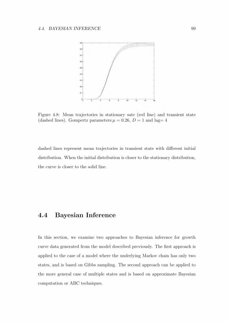
4.4. BAYESIAN INFERENCE 99
Figure 4.8: Mean trajectories in stationary sate (red line) and transient state(dashed lines). Gompertz parameters:µ = 0.26, D = 1 and lag= 4
dashed lines represent mean trajectories in transient state with different initial
distribution. When the initial distribution is closer to the stationary distribution,
the curve is closer to the solid line.
4.4 Bayesian Inference
In this section, we examine two approaches to Bayesian inference for growth
curve data generated from the model described previously. The first approach is
applied to the case of a model where the underlying Markov chain has only two
states, and is based on Gibbs sampling. The second approach can be applied to
the more general case of multiple states and is based on approximate Bayesian
computation or ABC techniques.

100 CHAPTER 4. STOCHASTIC MODELS
4.4.1 Gibbs Sampling approach for the two state model
with equal rates
Suppose that we observe single or multiple growth curve data at a series of time
points. Then in our model defined by (4.1) and (4.2), the likelihood function is
analytically unavailable, but for the case of two state in the Markov process Ut,
we can find an explicit expression for the likelihood when conditioning on the
initial state and the number of jumps in successive time intervals. This allows for
the implementation of a Gibbs sampling algorithm.
Formally, consider a continuous, time homogeneous Markov process with state
space S = 0, 1, where state transitions occur according to a Poisson process
with rate α. Suppose that bacterial population data are observed after fixed,
successive time points 0 < T1 < · · · < Tn. Then, the unknown parameters are
the Gompertz parameters and the rate parameter, α.
4.4.1.1 Estimation of the Gompertz parameters
Various approaches to estimation of the Gompertz parameters could be consid-
ered. A fully Bayesian approach would imply setting prior distributions to these
parameters as described in the previous chapters and then sampling from the
posterior conditional distributions within the MCMC algorithm. However, here,
for simplicity, we prefer to use a classical approximation. Recall firstly that under
the assumption that the process is in equilibrium initially, then from (4.7), the
mean trajectory is E[Yt] = 12G(t). Therefore, we propose to use standard, classi-
cal weighted mean squares techniques to estimate these parameters by fitting the
scaled Gompertz curve to the mean trajectory at the sample data time points.
The Gompertz parameters are assumed known for the remainder of the anal-

4.4. BAYESIAN INFERENCE 101
ysis. This implies that the overall approach to inference in this case is a form
of empirical Bayes analysis combining both classical and Bayesian estimation
techniques, see e.g Cassella (1985).
4.4.1.2 Estimation of α
Suppose now that the Gompertz parameters are known. Then, the time transfor-
mation is carried out the Gompertz function with known parameters as in (4.2).
From (4.1), the observed data are y = (y1, . . . , yn) where yi = ti1 is the total
(transformed) time spent in state 1 in interval i, so that G(Ti)−G(Ti−1) = t0i+ti1
where ti0 is the corresponding (transformed) time in interval i spent in state 0.
To compute the conditional likelihood function we will use the concept of
random division of an interval which we briefly present below following David
and Nagaraja (2003).
Random division of an interval
Suppose that n points are dropped at random on the unit interval (0, 1). The
ordered distances of these points from the origin are denoted by u(i) (i = 1, 2, ..., n)
and let wi = u(i) − u(i−1) (u(0) = 0) be the interval of time between them. Then
the random variables U(1), U(2), ..., U(n) are distributed as n order statistics from
a uniform U(0, 1) parent, that is, with joint pdf equal to n! over the simplex
0 ≤ u(1),≤ u(2),≤ ..., u(n) ≤ 1. Correspondingly, the pdf of the wi is
f(w1, w2, . . . , wn) = n! wi ≥ 0,n∑j=1
wj = 1. (4.9)

102 CHAPTER 4. STOCHASTIC MODELS
The distribution is completely symmetrical in the wi. Indeed, if we define
wn+1 = 1−n∑j=1
wj, (4.10)
we have the (degenerate) joint probability density function (j = 1, 2, ..., n, n+ 1)
f(w1, w2, ..., wn, wn+1) = n! wi ≥ 0,n+1∑j=1
wj = 1, (4.11)
which is still symmetrical in all sj. It follows that the joint distribution of any k
of the Wj(k = 1, 2, ..., n) is the same as that of the first k, and in particular that
the distribution of the sum of any k of the Wj is that of
U(k) = W1 +W2 + ...+Wk, (4.12)
namely
fUk(u) =
1
B(k, n+ 1− k)uk−1(1− u)n−k 0 ≤ u ≤ 1. (4.13)
The Wjs are commonly referred to as spacings.
The random division of the interval may in fact originate from a Poisson
process, such as our problem, with events occurring in some interval of time.
Then, the distribution of the k’th order statistic, Uk, in the interval [0, T ] is a
scaled beta distribution, B(k, n+ 1− k):
fUk(u) =
1
B(k, n+ 1− k)
uk−1(T − u)n−k
T n0 ≤ u ≤ T. (4.14)

4.4. BAYESIAN INFERENCE 103
Calculating the likelihood function
Suppose that we know the initial state, say s1, at the start of the first time
interval, and the number of state changes that occur in each time interval, say
Ni for i = 1, . . . , n. Then, the likelihood function is:
f(y|α, s1, N1, . . . , Nn) =n∏i=1
f(yi|α, si = mod(si−1 +Ni−1, 2), Ni) (4.15)
where mod(a, b) represents a modulo b, that is the densities of each yi are condi-
tionally independent given the state at the start of interval i and the number of
state transitions in the interval.
Now consider two cases: when Ni is odd and when Ni is even. Consider now
the different time intervals in each state.
• If Ni is odd, the process spends half of the time intervals in state 1 and the
remainder in state 0 and therefore, the distribution of the sum of (Ni+1)/2
intervals is equal to the distribution of the order statistic U((Ni+1)/2) as
defined in (4.14), that is:
f(yi|Ni, α) =1
B(Ni+12, Ni+1
2)
y(Ni+1)/2−1i (Ti − yi)(Ni+1)/2−1
TNii
(4.16)
• Ni even
As the number of time intervals in period i is odd, the process spends
Ni/2 + 1 time intervals in state 1 if the initial state is 1, or Ni/2 if the
initial state is 0. Therefore, from (4.14),
f(yi|si, Ni, α) =1
B(Ni
2+ si,
Ni
2+ (1− si)
yNi/2+si−1i (Ti − yi)Ni/2−si
TNii
(4.17)

104 CHAPTER 4. STOCHASTIC MODELS
4.4.1.3 Conditional posterior distributions
Assume that α has a gamma prior distribution, say α ∼ G(a, b). Then we have:
f(α|y, s1, N1, . . . , Nn) ∝ f(y|α, s1, N1, . . . , Nn)f(α|s1, N1, . . . , Nn)
∝ f(α|N1, . . . , Nn)
∝ f(N1, . . . , Nn|α)f(α)
∝n∏i=1
αNie−α(G(Ti)−G(Ti−1))αa−1e−bα
α|y, s1, N1, . . . , Nn ∼ G(a+ nN, b+ nT )
where N = (1/n)Σni=1Ni and T = (1/n)
∑ni=1(G(Ti) − G(Ti−1)) is the average
length of the transformed time intervals.
Latent variables Ni
f(Ni|y, s1,N−i, α) ∝ f(y|α, s1, N1, . . . , Nn)f(Ni|N−i, α)
∝ f(y|α, s1, N1, . . . , Nn)(α(G(ti)−G(ti−1)))Ni
Ni!
The posterior distributions of the Nis do not have a simple closed form and
we use a Metropolis-Hastings algorithm to sample from these distributions based
on generating candidate values from a Poisson distribution centred at the current
value plus 0.5.

4.4. BAYESIAN INFERENCE 105
Latent variable s1
Assume that s1 has a Bernoulli prior distribution, say P (s1 = 1|p) = p. Then,
f(s1|y, N1, . . . , Nn, α) ∝ P (s1)f(y|α, s1, N1, . . . , Nn)
∝n∏1
1
B( Ni
2+ s1,
Ni
2+ (1− s1))
yNi/2+s1−1i (Ti − yi)Ni/2−s1
T Nii
P (s1)
∝n∏1
1
B( Ni
2+ s1,
Ni
2+ (1− s1))
ys1i (Ti − yi)−s1ps1(1− p)1−s1
∼ Bernoulli(p′)
where n is how many times the number of jumps in an interval was even, Ni =∑ij=1Nj and p′ = pn
∏(yi/(Ti−yi))
(1−p)n+pn∏
(yi/(Ti−yi)) .
Gibbs sampler
Given the posterior conditional distributions calculated previously, a Metropolis
Hastings within Gibbs sampler can be defined to sample the posterior distribution
of α as follows:
1. Initialize counter k=1 and set the initial values: α(0), s(0)1 and
N(0)
2. Generate α(k) ∼ G(a+ nN(k−1)
, b+ nT )
3. Generate s(k)1 ∼ B(p′)
4. Generate N(k)1 :
4.1 For all Ni, generate a candidate from the proposal distribution
Q(N(k−1)i |N (∗)
i ): N(∗)i ∼ P(N
(k−1)i + 0.5)
4.2 Generate U ∼ U[0,1] If U ≤ min1, P (N∗i )Q(N
(k−1)i |N(∗)
i )
P (N(k−1)i )Q(N∗
i |N(k−1)i )
, then N(k)i =

106 CHAPTER 4. STOCHASTIC MODELS
N∗i . If not, N(k)i = N
(k−1)i .
5. Change k = k+1 and return to step 2 until convergence is reached.
4.4.1.4 Example
Assuming that the intensity rate of the jumps is α = 10, we generated a five sets of
growth curve data with twenty observations, equally spaced over time. Assuming
that the process is in stationary state, Gompertz parameters were estimated by
non-linear least squares and fixed when implementing the Gibbs sampling to
estimate α. We generated a sample of 20000 iterations, after a burn in period
of equal size. Looking at the plot of the cumulative mean of the sampled values
of α, on the left hand side of Figure 4.9, we see that the chain has converged
convergence. On the right hand side, we see the posterior distribution of α which
is centred on the true value. The posterior mean of α is equal to 9.791 and the
median is 9.705. A 95% credible interval is equal to (7.36, 12.85).
4.4.2 Approximate Bayesian Computation
When considering the general case of our model, with more than two states in
the Ut process, it is not clear that a similar expression for the likelihood can be
found as in the two state case. Therefore, the Gibbs sampling algorithm described
previously cannot be implemented and instead, we suggest applying approximate
Bayesian computation (ABC).

4.4. BAYESIAN INFERENCE 107
0 5000 10000 15000 20000
78
910
iteration
post
erio
r m
ean
(a) Cumulative mean
6 8 10 12 14 16
0.00
0.05
0.10
0.15
020
0.25
N = 20000 Bandwidth = 0.1736
Pos
terio
r de
nsity
of l
ambd
a(b) Posterior density
Figure 4.9: Trace plot and posterior density of α
4.4.2.1 A brief review of ABC
In many complex models, the likelihood function is unknown or intractable which
makes the implementation of standard Bayesian algorithms such as MCMC im-
possible. However, in some of these cases, it may be much more straightforward
to simulate data from the model. In these cases, ABC can be used to provide
an approximation of the posterior distribution. In a nutshell, in this approach,
parameter values are simulated from the prior distribution and then data are
simulated from the model conditional on these parameters. Then a similarity
criterion between the simulated and observed data is defined as an appropriate
distance between some summary statistics computed on both data sets. Param-
eters which generate data sufficiently similar to the sample data are accepted.
For fuller reviews in the ecological and genetic contexts see Beaumont (2010) and
Lopes and Boessenkool (2010).
ABC was originally developed to perform population genetics analysis (Tavare

108 CHAPTER 4. STOCHASTIC MODELS
et al. (1997) and Pritchard et al. (1999)), but recently it is being applied in a wide
range of fields, such as ecology, epidemiology, molecular evolution, conservation
genetics, etc. The increasing popularity on this method is due mainly to its
capability to deal with very complex models and high dimensional data via the
use of Monte Carlo simulations that avoid the need to use explicit likelihood
functions.
Assume that we have a model parameterized by θ. Then the basic algorithm
can be written as follow:
1. Sample a value of the model parameter from the prior distribution:
θ(i) ∼ f(θ)
2. Simulate data from the model, given θ(i): D(i) ∼ f(D|θ(i))
3. Summarize D(i) with a set of chosen summary statistics S(D(i))
4. Reject θ(i) if d(S(D(i)),S(y)) ≥ ε
5. Repeat until required number of candidates accepted.
where D are the simulated data, y is the observed data, d is a measure of
distance, S is some summary statistic and ε > 0 is a tolerance level. When ε
tends to zero, the algorithm provides a sample from the distribution f(θ|S(y)
which is an approximation of the desired distribution. If the summary statistic
S is sufficient, the f(θ|S(y)) = f(θ|y).
Recently, in the literature a number of modifications have been proposed
to improve the basic ABC algorithm. Firstly, Beaumont et al. (2002), propose
a regression method to improve the sampling of the posterior density. Their
algorithm introduces two innovations: weighting the parameters, θi, according to

4.4. BAYESIAN INFERENCE 109
their distance from the real data and adjusting the θi using local-linear regression
to weaken the effects of that discrepancy.
Secondly, in the absence of of prior information flat distribution should be
used. However, if the prior distribution is diffuse then many improbable param-
eter values can be generated so that the acceptance rate of the algorithm will
be very low and the algorithm becomes very inefficient. One possibility to over-
come the problem of inefficiency in that cases is to use a sequential algorithm
as proposed by S.A. et al. (2007) and Toni et al. (2009). The idea is to run the
ABC method using a rough estimate of the ith posterior as the (i + 1)th prior.
As the number of iterations increases the posterior distribution becomes sharper
and located closer to the true value.
The third main modified version of the ABC method is MCMC-ABC, pro-
posed in Marjoram et al. (2003). This algorithm starts by sampling from the
prior f(θ) and then a new value of the parameter is proposed using a proposal
distribution which depends on the current value of the parameter, K(θ|θi−1) .
If the parameter value holds the ABC rejection step (d(S(D(i)),S(y)) ≤ ε) and
then, the Metropolis rejection step, the proposed value is accepted.
4.4.2.2 Implementation of ABC
Consider now the general model with state space S = s1, . . . , sk and rates α, β
and known Gompertz parameters for simplicity. Assume gamma prior distri-
butions for the intensity rate parameters, α, β. Assume that we observe data,
y.
Then the ABC algorithm proceeds by simulating parameter values and then
simulating growth curve data at the same time points as the observed data given

110 CHAPTER 4. STOCHASTIC MODELS
these parameter values as follows.
1. Sample from the prior: α(i), β(i) ∼ G(a, b)
2. Simulate data given α(i), β(i): y(i) ∼ f(y|λ(i))
3. Reject α(i), β(i) if d(y(i),y) ≥ ε, where d(y(i),y) =∑n
j=1 wi|y(i)j − yj|
4. Repeat until required number of candidates accepted.
In the case where a single curve is observed, the weights are set to be equal.
When the observed data consist of several replications of the same process, sim-
ulated data is evaluated by taking into account its distance with respect to the
mean curve. The weights then aim to account for the variability of the process at
different point of times. For instance, as was said previously, replications of the
growth curve show less variability at the beginning of the observation period and
more variability as time evolves. Thus, our weights are computed to be inversely
proportional to the maximum distance observed at each point of time. After
that, we accept the 1% of the generated values of α, β, with the lowest distance
between the observed and simulated data.
Note that although we do not detail this here, the implementation of the
algorithm in the case of unknown Gompertz parameters does not present any
extra difficulties. These parameters can also be simulated from the prior and the
same distance measures as above can also be used.

4.4. BAYESIAN INFERENCE 111
Figure 4.10: Simulated data
4.4.2.3 Example I
We simulated a set of 20 curves, each with 16 observations at equal point of
times. Data was generated by assuming that the intensity rate is α = β = 1,
the growth rate of the Gompertz function is 0.26, the lag parameters is 4 and
the maximum population growth is 1. The Markov chain has only two states,
S = 0.8, 1. The simulated data are shown in Figure 4.4.2.3. The thick black
line is the mean curve that we will use to compute the distance in the rejection
step of the algorithm.
We assume gamma prior distributions for all the parameters due to their are
non-negative. The prior distribution for the intensity rate is α ∼ G(1, 1), and for
the Gompertz parameters the gamma prior distributions have means equal to the
least squares estimated values and variance 1. Finally, we compute the relative
mean integrate square error (RMISE) to set the number of iterations needed:

112 CHAPTER 4. STOCHASTIC MODELS
Table 4.1: Parameter estimates and RMISE
Numer of iterations Lambda Mu Lag D RMISE10000 0.99953 0.29589 4.18890 0.97269 0.0022350000 0.99704 0.27122 3.98730 1.01920 0.00055100000 1.00230 0.25849 4.00960 1.01730 0.00098500000 1.00170 0.26529 4.00120 1.01460 0.00097
True value 1 0.26 4 1
RMISE =1
N
N∑i=1
((θi − θ)2
θ2) (4.18)
where N is the number of sampled points from the posterior distribution, θi is
the ith sampled point from the posterior distribution of the parameter and θ is
the true value of the parameter. Results are shown in Table 4.1.
We see that RMISE seems to have stabilized after around 100000 iterations.
We can see also that estimations are very closed to the true values of the param-
eters.
4.4.2.4 Example II
Now, we will apply the ABC method to the Listeria monocytogenes data de-
scribed previously. In this case, we consider twenty growth curves, with sixteen
equally spaced observations in each case shown on the right hand side of Fig-
ure 4.5. Given the previous simulated example, we think that 100000 points are
enough to perform the analysis and we keep the 1h best. The left hand side of
Figure 4.11 shows the total curves that ABC method generates, and on the right
the the curves kept after the rejection step, that is the curves which have less
distance to the mean observed curve (central thick black line). The right hand
side of Figure 4.11, the plot also shows the maximum and the minimum observed

4.4. BAYESIAN INFERENCE 113
(a) All curves generated with ABC (b) The best 1h of the curves.
Figure 4.11: All and the best 1% of the generated curves
Table 4.2: Parameter estimates given different state spaces
S = 0.8, 1 S = 0.8, 1, 1.2 S = 0.8, 1, 1.2, 1.4 S = 0.8, 0.9 S = 0.8, 0.9, 1 S = 0.8, 0.9, 1, 1.1α 0.96 1.00 0.99 1.00 1.00 0.99µ 0.28 0.28 0.27 0.28 0.26 0.29
lag 3.88 3.90 3.87 3.89 3.80 3.93D 1.07 1.03 1.04 1.09 1.10 1.08
curves (thick black lines) to see that the simulated curves obtained from the ABC
show a variability similar to that observed with the real data.
The posterior means of the Gompertz function are equal to µ = 0.27616,
lag= 3.8859 y D = 1.0734 and posterior mean of the intensity rate is equal to
λ = 0.96261. Posterior densities are shown in Figure 4.12
Finally, we repeat the analysis but considering different state spaces for the
underlying Markov process. Results are presented in table 4.2. The results do not
change significantly among the different cases. Therefore, based on the Occam’s
razor principle we prefer the simpler model.

114 CHAPTER 4. STOCHASTIC MODELS
(a) Growth rate parameter (b) Lag parameter
(c) Maximum population growth (d) Intensity rate of jumps
Figure 4.12: Posterior means
4.5 Conclusions
In this chapter, we have presented a new, continuous time model for bacteria
growth based on a stochastic generalization of the Gompertz curve. We have
shown that our model can simulate data that show similar characteristics to
real bacteria growth data and have also developed two approaches to Bayesian
inference for our model based on both exact and likelihood free approaches.

Chapter 5
Extensions
Here we present various extensions of the ideas proposed in this thesis and some
further avenues for future research. In Section 1, we consider extensions of the
ideas introduced in Chapter 3 to the case of interacting populations. Secondly,
in Section 2, we briefly comment on an application of these ideas outside of the
area of bacterial growth to the development of a neural network based software
reliability model. Finally, in Section 3, we present some further extensions of our
work.
5.1 Predator prey modeling
The models proposed in this dissertation study the case of populations growing
in isolation. Nevertheless, in reality, populations interact with other species. In
particular, in the context of microorganisms, ?? introduce a general model for
interactions between prey and predator populations based on the Lotka-Volterra
115

116 CHAPTER 5. EXTENSIONS
model of (1.9) and (1.10).
dNdt
= N(t)f(N(t− δ))− g(N(t), P (t))P (t)
dPdt
= eg(N(t− τ), P (t− τ))P (t)− µP (t)
where N(t) and P (t) are the prey and predator population concentrations at time
t, f is the prey growth function, g represents the functional response relating the
reduction in prey population to current predator and prey population sizes, e is
a multiplicative constant reflecting the efficiency of the predator population in
reproduction, τ and δ are time lags and µ represents the death rate of predators.
Although in the literature there is agreement about the dynamical framework
of a predator-prey system, the explicit forms of the functional responses can be
highly controversial. ?? propose using splines to estimate the functions f and
g. Continuing the line of investigation of these authors, we propose using neural
networks, as in Chapter 3, to estimate the functional responses, f and g. To
illustrate, we have made a preliminary study applied to data on a protozoan
predator-prey interaction. Figure 5.1 shows the observed and estimated phase
trajectories of the predator-prey system in this case.
Further work is currently underway in this area.
5.2 Software reliability modeling
The non-parametric models proposed in Chapter 3, can be applied to many dif-
ferent fields, where the parameters of a primary model can be fitted as a function
of some given covariates using some form of non-parametric regression approach.
In particular, we have used these techniques in Wiper et al. (2012), to introduce
a simple parametric model for software failure where the failure rate depends on

5.2. SOFTWARE RELIABILITY MODELING 117
(a) Observed prey and predator evolution (b) Estimated prey and predator evolution
Figure 5.1: Estimated and observed phase trajectories
software metrics information and is modeled via neural networks. This is briefly
summarized below.
Consider the case where the times between successive software failures, say
T1, T2, . . . are observed and where it is presumed that the software is corrected,
possibly imperfectly, after each failure. Then, it is natural to assume a nonho-
mogeneous Poisson process for failures so that we model
Ti|λi ∼ Ex(λi) (5.1)
for i = 1, 2, . . .. Many standard software reliability models assume this basic ex-
ponential form. For instance, the Jelinski Moranda model (Jelinski and Moranda
(1972)) sets
λi = (N − i+ 1)µ
where N represents the number of faults in the original code, µ is the fault
discovery rate and perfect fault correction is assumed.

118 CHAPTER 5. EXTENSIONS
Suppose that after each software failure is observed, the code is modified and
software metrics such as lines of code or other complexity measures reflecting the
state of the code are evaluated. Then, we relate the failure rate of the software
to the software metrics as follows:
log λi = g(xi)
where xi = (xi1, . . . , xip)T are the metrics available after i− 1 failures have been
observed. Typically, the relation between the log failure rate and the metrics is
highly non linear and therefore, we proposed the use of a feed forward neural
network, that is:
g(x) = β0 +k∑j=1
βjΥ(γTj x
)where
Υ(c) = (1 + exp(−c))−1
and γj = (γj1, . . . , γjp)T .
The same prior structures as used in Chapter 3 are applied to the neural
network model and inference is again carried out using WinBUGS. Figure 5.2 taken
from Wiper et al. (2012) shows a set of Bayesian predictive intervals for numbers
of weekly software failures for a real data set consisting of the numbers of failures
in fourteen weeks where a similar, previous time period has been used as training
data. More details are available in this paper.
5.3 General extensions
In Chapter 2, we studied the case when various growth curves are observed under
the same identical conditions. The hierarchical model proposed was based on a

5.3. GENERAL EXTENSIONS 119
Figure 5.2: Observations (red circles), predictive mean values (blue circles) and95% credible intervals.

120 CHAPTER 5. EXTENSIONS
Gompertz curve, as this is one of the most widely applied primary models. A
natural extension is to apply the same ideas to alternative, parametric, growth
curve models such as the logistic or Baranyi models discussed in Chapter 1.
In particular, it would then be interesting to consider the problem of selection
between models using for instance the deviance information criterion. Equally,
the extension to varying environmental conditions via the neural network based
approach of Chapter 3 would also be interesting to explore for these alternative
models.
Secondly, outside of the laboratory, in real life, environmental factors such as
temperature may vary considerably throughout the storage and distribution time
of perishable foods. Therefore, another natural extension of our proposed models
of Chapter 3, is to consider the possibility that the environmental factors change
over time. Incorporating time-varying factors will lead to dynamical system.
The model we proposed in Chapter 4 should prove to be useful for other
applications where deterministic models are too restrictive and can not capture
the various sources of variations that exist in real life. Implementation for this
model was carried out using an empirical Bayes approach via a Gibbs sampler
for the case of a two state model and it is natural to see if a fully Bayes al-
gorithm which also fits the Gompertz parameters in a Bayesian way could be
developed. Secondly, for the general model, it is clear that many improvements
to the simple ABC algorithm we propose here could be possible. It would also be
interesting to incorporate the techniques of Chapter 3 in this model to allow us
to simultaneously study bacterial populations under different conditions. Finally,
the extension of our model to interacting populations should be of great interest
in several biological applications.

Bibliography
Andrieu, C., N. Freitas, and A. Doucet (2001). Robust full Bayesian learning for
radial basis networks. Neural Computation 13 (10), 2359–2407.
Augustin, J. and V. Carlier (2000). Modelling the growth rate of Listeria mono-
cytogenes with a multiplicative type model including interactions between en-
vironmental factors. International Journal of Food Microbiology 56 (1), 53–70.
Baranyi, J. (1998). Comparison of stochastic and deterministic concepts of bac-
terial lag. Journal of Theoretical Biology 192 (3), 403–408.
Baranyi, J., C. Pin, and T. Ross (1999). Validating and comparing predictive
models. International Journal of Food Microbiology 48 (3), 159–166.
Baranyi, J. and T. Roberts (1994). A dynamic approach to predicting bacterial
growth in food. International Journal of Food Microbiology 23 (3-4), 277–294.
Baranyi, J. and T. Roberts (1995). Mathematics of predictive food microbiology.
International Journal of Food Microbiology 26 (2), 199–218.
Beaumont, M. (2010). Approximate bayesian computation in evolution and ecol-
ogy. Annual Review of Ecology, Evolution, and Systematics 41, 379–406.
Beaumont, M., W. Zhang, and D. Balding (2002). Approximate bayesian com-
putation in population genetics. Genetics 162, 2025–2035.
121

122 BIBLIOGRAPHY
Brooks, S. and A. Gelman (1998). General methods for monitoring convergence of
iterative simulations. Journal of Computational and Graphical Statistics 7 (4),
434–455.
Buchanan, R., R. Whiting, and W. Damert (1997). When is simple good enough:
a comparison of the Gompertz, Baranyi, and three-phase linear models for
fitting bacterial growth curves. Food Microbiology 14 (4), 313–326.
Cassella, G. (1985). An introduction to empirical bayes data analysis. The
American Statistician 39, 83–87.
Celeux, G., F. Forbes, C. Robert, and D. Titterington (2006). Deviance informa-
tion criteria for missing data models. Bayesian Analysis 1 (4), 651–674.
Congdon, P. (2010). Applied Bayesian Hierarchical Methods. Chapman and Hall.
Cowles, M. and B. Carlin (1996). Markov Chain Monte Carlo convergence diag-
nostics: A comparative review. Journal of the American Statistical Associa-
tion 91 (434), 883–904.
David, H. and H. Nagaraja (2003). Order statistics (third ed.). Wiley.
Delignette-Muller, M., M. Cornu, R. Pouillot, and J. Denis (2006). Use of
Bayesian modelling in risk assessment: Application to growth of Listeria mono-
cytogenes and food flora in cold-smoked salmon. International journal of food
microbiology 106 (2), 195–208.
Donnet, S., J. Foulley, and A. Samson (2010). Bayesian analysis of growth
curves using mixed models defined by stochastic differential equations. Bio-
metrics 66 (3), 733–741.
Efron, B. and R. J. Tibshirani (1993). An introduction to the Bootstrap. New
York: Chapman & Hall.

BIBLIOGRAPHY 123
Fine, T. (1999). Feedforward neural network methodology. Springer Verlag.
Fitzmaurice, G., M. Davidian, G. Verbeke, and G. Mohlenbergs (2008). Longitu-
dinal Data Analysis. Chapman and Hall.
Garcıa-Gimeno, R., C. Hervas-Martınez, et al. (2002). Improving artificial neural
networks with a pruning methodology and genetic algorithms for their appli-
cation in microbial growth prediction in food. International Journal of Food
Microbiology 72 (1-2), 19.
Geeraerd, A., C. Herremans, C. Cenens, and J. Van Impe (1998). Application
of artificial neural networks as a non-linear modular modeling technique to
describe bacterial growth in chilled food products. International journal of
food microbiology 44 (1-2), 49–68.
Gelfand, A. (1996). Model determination using sampling-based methods. in w.
gilks, s. richardson, d. spiegelhalter (eds.). , Markov Chain Monte Carlo in
Practice, 145–161.
Gelfand, A. and S. Ghosh (1998). Model choice: a minimum posterior predictive
loss approach. Biometrika 85, 1.
Gelman, A. and D. Rubin (1992). Inference from iterative simulation using mul-
tiple sequences. Statistical Science 7, 457–511.
Geweke, J. (1992). Bayesian Statistics 4, Chapter Evaluating the accuracy of
sampling-based approaches to calculating posterior moments. Clarendon Press.
Gilioli, G., S. Pasquali, and F. Ruggeri (2008). Bayesian inference for functional
response in a stochastic predator-prey system. Bulletin of Mathematical Biol-
ogy 70 (2), 358–81.

124 BIBLIOGRAPHY
Gilks, W., S. Richardson, and D. J. Spiegelhalter (1996). Markov chain Monte
Carlo in practice. London: Chapman and Hall.
Gompertz, B. (1825). On the nature of the function expressive of the law of human
mortality, and on a new mode of determining the value of life contingencies.
Philosophical Transactions of the Royal Society of London 115, 513–583.
Grijspeerdt, K. and P. Vanrolleghem (1999). Estimating the parameters of the
Baranyi model for bacterial growth. Food Microbiology 16 (6), 593–605.
Hajmeer, M., I. Basheer, and Y. Najjar (1997). Computational neural networks
for predictive microbiology II. Application to microbial growth. International
journal of food microbiology 34 (1), 51–66.
Jelinski, Z. and P. Moranda (1972). Software reliability research. Academic Press.
Kery, M. (2010). Introduction to WinBUGS for Ecologists: Bayesian approach to
regression, ANOVA, mixed models and related analyses. Academic Press.
King, R., B. Morgan, O. Gimenez, and S. Brooks (2009). Bayesian Analysis for
Population Ecology. Chapman and Hall/CRC.
Lande, R., S. Engen, and B. E. Saether (2003). Stochastic populated dynamics in
ecology and conservation. Oxford University Press.
Lavine, M. and M. West (1992). A Bayesian method for classification and dis-
crimination. Canadian Journal of Statistics 20 (4), 451–461.
Lee, H. (2004). Bayesian nonparametrics via neural networks. Society for Indus-
trial Mathematics.
Levenberg, K. (1944). A method for the solution of certain non-linear problems
in least squares. Quarterly of Applied Mathematics 2, 164–168.

BIBLIOGRAPHY 125
Lopes, J. and S. Boessenkool (2010). The use of approximate bayesian computa-
tion in conservation genetics and its application in a case study on yellow-eyed
penguins. Conservation Genetics 11 (2), 421–433.
Lotka, A. J. (1925). Elements of Physical Biology. Baltimore: Williams and
Wilkins.
Lunn, D., A. Thomas, N. Best, and D. Spiegelhalter (2000). WinBUGS-a
Bayesian modelling framework: concepts, structure, and extensibility. Statis-
tics and Computing 10, 325–337.
MacKay, D. (1995a). Bayesian methods for neural networks: Theory and ap-
plications. Technical report, Cambridge: Cavendish Laboratory, Cambridge
University.
MacKay, D. (1995b). A practical bayesian framework for backpropagation net-
works. Neural Computing 4, 448–472.
Malthus, T. R. (1798). An Essay on the Principle of Population. Reprint (1998).
Amherst, NY: Prometheus Books.
Marjoram, P., J. Molitor, V. Plagnol, and S. Tavare (2003). Markov chain monte
carlo without likelihoods. Proceedings of the National Academy of Science of
the USA 100, 15324–15328.
Marquardt, D. (1963). An algorithm for least-squares estimation of nonlinear
parameters. SIAM Journal on Applied Mathematics 11, 431–441.
McCarthy, M. (2007). Bayesian Methods for Ecology. Cambridge University
Press.

126 BIBLIOGRAPHY
McKellar, R. (2001). Development of a dynamic continuous-discrete-continuous
model describing the lag phase of individual bacterial cells. Journal of Applied
Microbiology 90, 407–413.
McKellar, R. and X. Lu (2004). Modeling microbial responses in food. CRC Press.
Muller, P. and D. R. Insua (1998). Issues in Bayesian analysis of neural network
models. Neural Computation 10 (3), 749–770.
Muller, P. and D. Rios Insua (1998). Issues in Bayesian analysis of neural network
models. Neural Computation 10, 749–770.
Murray, J. D. (2003). Mathematical Biology. Berlin: Springer .
Neal, R. (1996). Bayesian learning for neural networks. Springer Verlag.
Pouillot, R., I. Albert, M. Cornu, and J. Denis (2003). Estimation of uncertainty
and variability in bacterial growth using Bayesian inference. Application to
Listeria monocytogenes. International journal of food microbiology 81 (2), 87–
104.
Powell, M., M. Tamplin, B. Marks, and D. Campos (2006). Bayesian synthe-
sis of a pathogen growth model: Listeria monocytogenes under competition.
International journal of food microbiology 109 (1-2), 34–46.
Pritchard, J., M. Seielstad, A. Perez-Lezaun, and M. Feldman (1999). Population
growth of human y chromosomes: a study of y chromosome microsatellites.
Molecular Biology and Evolution 16 (12), 1791–1798.
Ratkowsky, D., J. Olley, T. McMeekin, and A. Ball (1982). Relationship be-
tween temperature and growth rate of bacterial cultures. Journal of Bacteri-
ology 149 (1), 1.
BIBLIOGRAPHY 127
Renshaw, E. (2011). Stochastic Population processes: Analysis, Approximations,
Simulations. Oxford University Press.
Robert, C. and K. Mengersen (1999). Reparameterisation issues in mixture mod-
elling and their bearing on MCMC algorithms. Computational Statistics and
Data Analysis 29 (3), 325–344.
Roeder, K. and L. Wasserman (1997). Practical Bayesian density estimation using
mixtures of normals. Journal of the American Statistical Association 92 (439),
894–902.
Rosso, L., J. Lobry, and J. Flandrois (1993). An unexpected correlation between
cardinal temperatures of microbial growth highlighted by a new model. Journal
of Theoretical Biology 162 (4), 447–463.
Russo, T., P. Baldi, A. Parisi, G. Magnifico, S. Mariani, and S. Cataudella (2009).
Levy processes and stochastic von bertalanffy models of growth, with applica-
tion to fish population analysis. Journal of theoretical biology 258 (4), 521–529.
S.A., S., Y. Fan, and M. Tanaka (2007). Sequential monte carlo without likeli-
hoods. Proceedings of the National Academy of Science 104, 1760–1765.
Seber, G. and C. Wild (1989). Nonlinear regression. Wiley.
Spiegelhalter, D., N. Best, B. Carlin, and A. van der Linde (2002). Bayesian
measures of model complexity and fit. Journal of the Royal Statistical Society.
Series B, Statistical Methodology 64 (4), 583–639.
Stern, H. (1996). Neural networks in applied statistics. Technometrics 38 (3),
205–214.
Tavare, S., D. Balding, R. Griffiths, and P. Donnelly (1997). Inferring coalescence
times from dna sequence data. Genetics 145 (2), 505.

128 BIBLIOGRAPHY
Taylor, H. and S. Karlin (1998). An Introduction to Stochastic Modeling: 3rd
edition. Academic Press.
Toni, T., D. Welch, N. Strelkowa, A. Ipsen, and M. Stumpf (2009). Approximate
bayesian computation scheme for parameter inference and model selection in
dynamical systems. Journal of the Royal Society Interface 6, 187–202.
Turchin, P. (2003). Complex Population Dynamics: A Theoretical/empirical Syn-
thesis. Princeton University Press.
Vehtari, A. and J. Lampinen (2003). Expected utility estimation via cross-
validation. Bayesian statistics 7, 701–710.
Verhulst, P. F. (1838). Notice sur la loi que la population suit dans son accroisse-
ment. Correspondance Mathematique et Physique 10, 113–121.
Volterra, V. (1926). Fluctuations in the abundance of a species considered math-
ematically. Nature 118 (558-60).
Wijtzes, T., J. De Wit, I. Huis, R. Van’t, and M. Zwietering (1995). Modelling
bacterial growth of Lactobacillus curvatus as a function of acidity and temper-
ature. Applied and environmental microbiology 61 (7), 2533.
Wiper, M., A. Palacios, and J. Marın (2012). Bayesian software reliability pre-
diction using software metrics information. Quality Technology & Quantitative
Management 9, 35–44.
Zwietering, M., T. Wijtzes, J. De Wit, and V. R. K. (1992). A decision sup-
port system for prediction of the microbial spoilage in foods. Journal of Food
Protection 55, 973–979.