ana marta rodrigues dos santos - ulisboa
TRANSCRIPT

Hydrodynamic analysis of a slalom fin of windsurf board
Ana Marta Rodrigues dos Santos
Thesis to obtain the Master of Science Degree in
Naval Architecture and Marine Engineering
Naval Architecture and Ocean Engineering
Supervisor: Prof. José Manuel da Silva Chaves Ribeiro Pereira
Co-Supervisor: Prof. Yordan Garbatov
Examination Committee
Chairperson: Prof. Carlos Guedes Soares
Member: Prof. Yordan Garbatov
Member: Prof. Sergey Sutulo
December 2018

ii

iii
"“Difficult” and “impossible” are cousins often mistaken for one
another, with very little in common."
- Scott Lynch, Red Seas Under Red Skies
"Why do we love the sea? It is because it has some potent power to
make us think things we like to think."
- Robert Henri

iv

v
Acknowledgements
There is a handful of people who made this sailing on stormy seas much easier. Some helped guiding
the ship, like: Professor José Chaves Pereira, for his extensive knowledge and clearness in teaching that
makes it easy to understand complex problems; Professor Yordan Garbatov, for lighting my interest on
the subject and helping this thesis turn into a practical application, which I like; and Dr Leigh Sutherland,
that was always kind and interested in helping, tying ends in different disciplines to take the projects to
the next level. To Luis Baptista at Vera Navis, with whom discussing these matters was always like
exploring. As my employer, he was enduringly understanding of the situation and granted me the space
and time to arrive to port. To the people working at LASEF, specially Duarte, for advice and help. To
all them, my thanks for the time and guidance.
To my friends at college, Nir and Gorka, for being good mates and for their efforts in the many
endeavours. If not for them, these two years would had been boring. It was a pleasure sailing with them.
À minha familia, pela oportunidade de estudar e chegar ao lugar onde estou. Obrigada por todo o apoio
e por me levarem sempre em frente, são os melhores pais que podia desejar.
And to my partner and best friend, Francisco, for always believing in me. For the many times we couldn’t
be together because of college, for the many times he gave me stamina to finish though projects, for
always being caring and understanding, this is for you: it’s done, let’s go!

vi

vii
Abstract
The objective of the thesis is to perform a hydrodynamic analysis in estimating the water-induced loads
on a real slalom fin of a windsurf board. First, an initial 2-D flow study of the fin hydrofoil, using the
software XFOIL will be performed. This will serve as mean of calibration for the commercial
Computational Fluid Dynamics software Star-CCM+. Since the analysed flow is in the range of 3x10⁵
to 10x105 of the Reynolds' number, inside the transition interval, laminar, transition and turbulence
models will be used. The 2-D flow study of the hydrofoil and the 3-D flow study of the fin will be
conducted using Star-CCM+, to analyse the fluid-structure interaction. This MSc thesis will rely on
several research collaborations originating from different Universities from Portugal and the United
Kingdom, which may lead to an opportunity of a further cavitation phenomenon investigation.
Keywords: CFD, Star-CCM+, Windsurf, Fin, RANS, Hydrofoil, γ – Reθ transition model, k – ω SST

viii

ix
Contents
Acknowledgements v Abstract vii Contents ix List of Tables xi List of Figures xiii Nomenclature xv Glossary xvii Chapter 1 Introduction 1
1.1 Motivation 1
1.2 Objectives 1
1.3 Thesis Structure 2
1.4 Conceptualisation and State-of-the-Art 2
Chapter 2 Slalom Fin of Windsurf Board 7
2.1 Work Description 7
2.2 Bibliographic Revision 7
2.3 Work Case Studies 8
2.4 Fin Design and Physical Properties 8
2.5 Aerofoils 9
2.6 Navier-Stokes and CFD Analysis 11
2.7 Boundary Layer 13
Chapter 3 Preliminary Analysis 15
3.1 Initial Considerations 15
3.2 Pre-Analysis Software Selection 15
3.3 Case Study 1 17
3.3.1 Initial Stage 19
3.4 Analysis 21
3.5 Case Study 2 22
3.6 Results Discussion 23
Chapter 4 Mesh, Turbulence and Transition Model 27
4.1 CFD Software Selection 27
4.2 Star-CCM+ Aerodynamic Models 28
4.2.1 SST k – ω Turbulence Model 28
4.2.2 γ – Reθ Transition Model 29
4.3 Mesh Characteristics 29
4.4 Case Study 3 31
4.5 Validation Conclusions 36

x
Chapter 5 SFWB Profile Performance 37
5.1 Case Study 4: SFWB Results 37
5.2 Mesh Convergence Study 43
5.3 General Conclusions 45
Chapter 6 SFWB Operation 47
6.1 Physical models and mesh considerations 47
6.2 SWBD Three-Dimensional Aerodynamic Analysis 49
6.3 General SFWB Conclusions 52
Chapter 7 Additional Studies 53
7.1 Parametric Optimisation Study 53
7.1.1 5% Thickness Variation 53
7.1.2 Maximum Thickness Position Variation 55
7.1.3 Conclusions 56
7.2 User Profiles 56
7.3 Notes on Water Tunnel Results 58
Chapter 8 Conclusion 59 Chapter 9 Future Work 63 References 65 Appendix A 69 A.1 P113 Coordinates 69

xi
List of Tables
2.1 Trial running parameters 9
3.1 thickness and location of maximum thickness along the fin 18
4.1 domain and control volumes’ dimensions 30
4.2 domain and control volumes’ mesh parameters 30
5.1 SFWB two-dimensional mesh parameters 44
6.1 domain and control volumes' dimensions for 3-D solution 48
7.1 Pressure values for velocity vs AoA 57
7.2 Event probability of an event for each user 57

xii

xiii
List of Figures
1.1 S. Newman Darby steering sailboard backwards on Susquehana River, Pennsylvania (1964) 3
1.2 Modern windsurf board 3
1.3 Diagram of the different features of a windsurf board 4
1.4 From left to right: race fin, slalom fin and wave fin (images by EASY/SURF) 5
2.1 Slalom Windsurf board fin dimensions (all dimensions in mm and degrees) 8
2.2 Different aerofoils and hydrofoils (Wikipedia images) 10
2.3 Aerofoil/hydrofoil terminology 10
2.4 Flow lines around the profile get closer on the upper surface (negative pressure distribution),
and apart on the lower surface (positive pressure distribution) 10
2.5 Laminar and turbulent boundary layers exemplificative diagram and respective development
of the velocity profiles [1] 14
2.6 Laminar separation bubble 14
3.1 Location of the three profiles to be studied, named P1, P2 and P3 17
3.2 hydrofoil P1 at plane 1, 100 mm from root 17
3.3 hydrofoil P2 at plane 2, 200 mm from root 18
3.4 hydrofoil P3 at plane 3, 300 mm from root 18
3.5 Comparison between original hydrofoils and NACA 0008 18
3.6 Pressure coefficient distribution from p1 19
3.7 Comparison between original coordinates from SFWB and the faired hydrofoil 20
3.8 Pressure coefficient distribution from profile P113 at Re 0.46 x10⁶ and AoA 0° 20
3.9 Pressure coefficient distribution from profile NACA 0008 at Re 0.46 x10⁶ and AoA 0° 21
3.10 Eppler 387 foil (in pink) 22
3.11 Plots for the Cl, Cd and Cm coefficients on E387, using Nasa wind tunnel results and XFOIL
results 23
3.12 Plots for the Cl, Cd and Cm coefficients and transition coordinates on P113, XFOIL results 24
4.1 Mesh definition 31
4.2 E387 lift and drag coefficients results from STAR-CCM+, XFOIL and Wind-tunnel
experiments 33
4.3 Intermittency for the aerofoil E387, AoA 4°, γ – Reθ 34
4.4 Turbulent Kinetic Energy for the aerofoil E387, AoA 4°, k – ω SST and γ – Reθ 34
4.5 Turbulent Kinetic Energy for the aerofoil E387, AoA 4°, k – ω SST 34
4.6 Transition curves for E387, XFOIL vs k – ω SST + γ – Reθ 35
4.7 E387 pressure distribution, AoA 0°, γ – Reθ 36
5.1 Lift coefficient monitor, Re 7.5 x10⁵, 8° AoA 38
5.2 Variance of Pressure for the complete simulation, Re 7.5 x10⁵, 8° AoA 38
5.3 Q-Criterion for converged solution, Re 7.5 x10⁵, 8° AoA 38
5.4 Transition curves for P113, XFOIL vs k – ω SST + γ – Reθ., Re: 5 x10⁵ 39
5.5 Turbulent Kinetic Energy for the hydrofoil P113, AoA 0°., Re: 5 x10⁵, k – ω SST γ – Reθ 40

xiv
5.6 Turbulent Kinetic Energy for the hydrofoil P113, AoA 4°., Re: 5 x10⁵, k – ω SST γ – Reθ 40
5.7 Velocity vector line display for the hydrofoil P113, AoA 4°., Re: 5 x10⁵, k – ω SST γ – Reθ 41
5.8 Lift coefficient and LSB length in chord percentage for AoA spectrum, Re: 5 x10⁵, k – ω SST
γ – Reθ 41
5.9 Pressure Coefficient for the hydrofoil P113, AoA 4°, k – ω SST γ – Reθ 43
5.10 Intermittency for the hydrofoil P113, AoA 4°, k – ω SST γ – Reθ 43
5.11 Results for Cl and Cd for different meshes 45
6.1 3-D Control Volumes 48
6.2 LSB at the Fin, Re: 5.0 x10⁵, 0° AoA 49
6.3 Fin Ox Pressure curves for AoA = 0° 50
6.4 Comparison between 2-D and 3-D results: Pressure 50
6.5 Turbulent Kinetic Energy (blue) and LSB (red) 51
6.6 Skin Friction (gradient) 51
6.7 Streamlines at 0° AoA 52
7.1 Results for +5% thickness modification 54
7.2 Results for -5% thickness modification 54
7.3 Results for +5% thickness position modification 55
7.4 Results for -5% thickness position modification 56
7.5 Weibull Distribution for the three user profiles 58

xv
Nomenclature
• U - Velocity
• AoA or α – Angle of Attack
• Cl or CL – Lift Coefficient
• Cd or CD – Drag Coefficient
• Cm or CM – Moment Coefficient
• L – Lift Force
• D – Drag Force
• M - Moment
• p – Pressure
• ρ – Specific Density
• S – Wing area
• c – Chord
• T – Temperature
• Pr – Prandtl number
• q – Heat Flux
• τ – Stress Tensor

xvi

xvii
Glossary
• CFD – Computational Fluid Dynamics
• SFWB – Slalom Fin of Windsurf Board
• FSI – Fluid Structure Interaction
• LSB – Laminar Separation Bubble
• N-S – Navier-Stokes
• US – Upper Surface
• LS – Lower Surface
• TKE – Turbulent Kinetic Energy

xviii

1
Chapter 1
Introduction
1.1 Motivation
Since the early ages, man has designed and crafted vessels that would help on the task of crossing
seas, rivers and oceans. Nowadays, man no longer needs to build for the sole purpose of survival:
he can use his crafts for leisure as well. At the marine environment, there are several sports and
amusements which require the art and know-how skills of artisans, be it windsurf surfboards or
small sailing crafts. With modern technology, it is within reach an in-depth engineering study of
these crafted arts. Together in symbiosis, art and engineering may lead to improved performance,
taking man faster and further into the future.
This thesis aspires to open a door in the study of crafted windsurf board fins, where an already
existing design will be studied and dissected. With the tools available in our century, the flow and
fluid-structure interaction can be simulated with accuracy, to pinpoint the aspects of the part that
can be improved. Specifically, these tools would be Computational Fluid Dynamics’ (CFD),
software, a virtual environment where the fin can be pushed to the limits endlessly and at lower
costs than those of a towing tank.
1.2 Objectives
This thesis performs a hydrodynamic analysis to a slalom fin for a windsurf board (SFWB). The
fin, object of the study, is made by F-Hot company, by the designer Steve Cook. The primary
objective includes:
• Verify the pressure distribution at the slalom fin of windsurf board.
Aside from the present work, an approach using numerical and experimental analysis to the
ultimate strength of the SFWB is being conducted. In the future, the following studies will be
performed [2]:
2
• Fluid-Structure Interaction (FSI) modelling (using data provided with this thesis, to be
developed at Instituto Superior Técnico);
• Fin optimisation, using the previously developed models as a design tool;
The creation of a foil for marine sports’ applications covers many steps, like the structural
engineering, the hydrodynamics, durability, fatigue, etc. Despite the comprehensive checklist, the
study will focus on the analysis of the flow around the SFWB. It is intended to understand how
the flow will develop inside a velocity envelope, and what will be the hydrodynamic loads on the
structure. As such, the fin will first be studied in 2-D, where validation of results can be easily
assessed. After, the study will be carried out in 3-D.
1.3 Thesis Structure
Chapter 1 presents the introduction of the studied problem. The second chapter will polish the
problem and introduce basic aerodynamic concepts to help understand later the results. The third
chapter describes a preliminary analysis to the 2-D aerofoil: this would validate later the results
from the CFD software, as well as give a first glimpse of the phenomena taking place.
Chapter 4 describes the selection of the parameters for the CFD analysis and its validation by
wind-tunnel data, to be later used on the subjects of Chapter 5 and Chapter 6. The proper 2-D
analysis of the fin profile is discussed in Chapter 5, and then Chapter 6 takes it to the third
dimension. To finalise, two studies have been added: one of parametric optimisation of the
hydrofoil and a second one, that shows the solicitation of the piece by three user types. It has also
been included some notes regarding the data obtained in the water tank, that may be found in
Chapter 7. Finally, Chapter 8 concludes all the investigation, and Chapter 9 discusses future work.
1.4 Conceptualisation and State-of-the-Art
By the beginning of the 20th century, pure sailing ships gave way to machine-powered vessels and
the primary propulsion method for trading and naval ships. However, sailing ships continued to
be appraised for recreational uses.
It was for that very purpose that in 1965, S. Newman Darby, an inventor, designed a hand-held
sail rig fastened with a universal joint to a floating platform with a tail fin (Figure 1.1). He would
name it of sailboarding, as published in Popular Science Monthly magazine. He would then
manufacture with his brothers these boards in Darby Industries, despite no patent associated.

3
Figure 1.1: S. Newman Darby steering sailboard backwards on
Susquehana River, Pennsylvania (1964)
Figure 1.2: Modern windsurf board
Sailboarding is nowadays known as windsurfing. The name was adopted from Windsurfer
International, a company owned by Hoyle Schweitzer and Jim Drake, developed through a patent
granted to them on 1970 for a wind-propelled apparatus, that, in essence, was a duplicate of
Newman Darby’s work of the sailboard.
Darby would win the rights for his invention years later, and continuously improve the windsurf
board (Figure 1.2). [3]
Now, windsurfing is commonly known as a surface water sport, joining the sailing and surfing
sports. The sailboard will navigate accordingly to the way the sailor manoeuvres the sail, using
the boom, and the wind conditions. As expected, the sail must be oriented from the leech to the
luff with the wind direction, with the sailor on the lee side. The balance between board, rig and
sailor is fundamental to keep sailing/hydroplaning.
The boards are usually 2.5 to 3 metres in length, keeping the rig and the universal joint as a
primary feature. The rig now consists of a mast, boom and sail (see Figure 1.3). Depending on
the user, conditions and type of windsurfing, the area of the sail may change. Furthermore, to give
rigidity to the sail, sometimes battens and batten pockets may be applied, much resembling the
Asian junk ship’s sails. As for the hull, main features consist on the mast track, where the universal
joint fits, the centreboard slit, for the centreboard (a type of retractable fin that is used to oppose
the drag force of the sail and sail upwind [4]), the foot straps on deck, to help the raider on
manoeuvres, and the piece in analysis on this thesis, the fin, or skeg.
The fin is firmly fitted on the bottom of the board, inside the water. Its primary purpose is to
generate lift and assist in the directional control of the board. Typically, the larger the fin, the
more lift it will generate, ideally for proportionally bigger sails and lighter winds. Smaller skegs
are good for strong winds, for a more manoeuvre sailing style or for taking the first steps on the
sport [5]. Thickness is also of importance, as thicker fins generate more power in light wind, but
are less efficient when the sailing speed increases. Finally, flexibility is another factor to have in

4
mind when choosing the sailing speed desired: if the fins are stiffer, higher speeds are efficiently
achieved, but when manoeuvring, malleable fins win.
Figure 1.3: Diagram of the different features of a windsurf board.
Of course, soon enough new branches of the sport were sprouting. The fins would also be adapted
to the new demands, being distinguished the main types of fins (see Figure 1.4 for some
examples):
• Race fins: Very long, straight and slim with maximum stiffness, made in carbon fibre.
• Slalom Fins: Shorter fins, but equally stiff and slim. May be tilted backwards, also made
in carbon fibre composites or G10.
• Freeride Fins: About the same length as the fins for slalom, but more flexible and with
a curved outline. Primary materials for the composition are carbon composites, G10 or
vinyl.
• Freestyle Fins: Wide, short fins, that provide fast planning and good acceleration, also
ensuring low resistance during sliding manoeuvres. Materials comprehend G10 or vinyl
composites.
• Wave Fins: Short and with a curved outline, are the most manoeuvrable fins, appropriate
for wave riding. Can be used in single or multiple fin configurations. Made of G10 or
Vinyl composites.

5
• Bump & Jump Fins: Fins made for sailing on smaller boards but with high winds, also
great for leaping, as they provide excellent control and speed, keeping manoeuvrability.
Made of G10 or vinyl composites.
• Anti-Weed Fins: These fins possess a highly tilted shape to promote the weed sliding,
where the conditions of the water demand. They can have many sizes to fit different
sailing styles.
• Shallow Waters’ Fins: Half of the length of regular fins, these fins are suited for very
shallow waters. As to compensate, the area of the fin increases with its broader and
thicker body. Primary materials are G10 or vinyl composites. [6]
Figure 1.3: From left to right: race fin, slalom fin and wave fin (images by EASY/SURF)

6

7
Chapter 2
Slalom Fin of Windsurf Board
2.1 Work Description
As windsurfing is becoming more and more a competitive sport (like Formula Windsurf, Slalom
competition, or even at the Summer Olympics, for example), there is also the need to amplify the
skills of the sailors. Such performance can be achieved with the improvement of characteristics
like weight, hull surface friction, sail camber, or, as it will be explored in this thesis, the fin
configuration.
Many aspects being materials, the arrangement of composite layers, shape or thickness can be
changed; nevertheless, the present aim concerns the nature of the hydrodynamic flow and the
estimation of the water-induced loads. The study of an existing slalom fin of windsurf board may
lead to a better understanding of its flaws, providing insight into the improvement of new fins.
2.2 Bibliographic Revision
The research of information needed to meet two subjects. First, it had to be a hydrodynamic or
aerodynamic study of a profile, and secondly, this study had to be centred on the same flow
conditions, specifically Reynolds number. Additionally, some publications are essential and other
bibliography is also recommended by the supervisors.
The main publication for aid in CFD analysis in this thesis was The Finite Volume Method in
Computational Fluid Dynamics, by F. Moukalled [7] while for the basics of aerodynamics is the
Fundamentos de Aerodinâmica Incompressível, by V. Brederode [8].
A similar dissertation suggested by the supervisors was done by N. Silva on Parametric Design,
Aerodynamic Analysis and Parametric Optimization of a Solar UAV [9]. This project has many
common points in what concerns the nature of the flow and physical models employed at the CFD
analysis. Another close project is developed by K. Atkins [10]. Finally, the present dissertation is

8
a continuation of the project developed by F. Nascimento on the numerical and experimental
analysis of ultimate strength for the windsurf fin [11].
2.3 Work Case Studies
The hydrodynamic analysis will be conducted using computational fluid dynamics. The case
studies for the analysis are:
1. To conduct a pre-analysis in 2-D, for a control aerofoil (E387) and the fin profile. A free
software will be used (XFOIL). This will depict a general idea of the range of values, for
pressure, lift, drag and other phenomena, to be expected per 3-D analysis;
2. Compare program data obtained for the control aerofoil to wind-tunnel results to verify
the legitimacy of the data;
3. After, using Star-CCM+, a 2-D analysis of the control profile E387 will be performed to
verify the physics models to employ, comparing to wind-tunnel and XFOIL data.
4. Using Star-CCM+, perform a 2-D flow analysis of the fin profile.
5. To finalise the research, the 3-D analysis of the complete fin will be run on Star-CCM.
2.4 Fin Design and Physical Properties
This chapter aims to establish all the parameters needed to start the analysis. As such, a description
of the slalom fin is necessary. After, the mission envelope, consisting on speed, sea parameters
(and thus Reynolds number), and angle of attack, will be characterised.
• 37 RS-3 Standard Slalom Fin
The object in the study is a slalom fin for windsurfing practice, as in Figure 2.1. The total span,
excluding the board attachment box, is of 360.17 mm. The length, or chord, at root is 100 mm,
the rake angle 2° to the aft.
Figure 2.1: Slalom fin of windsurf board dimensions (all dimensions in mm and degrees)

9
The leading edge of the piece is to be the round front, and the trailing edge the straight opposite
side. The F-Hot company produces the SFWB. Further analysis of the hydrofoil development is
carried out in Chapter 3: Preliminary Analysis.
• Trial Envelope
To perform the study on the SFWB, it is necessary to know the fluid characteristics. The table 2.1
summarises all the needed seawater parameters with a salinity of 35 g/kg [12] [13], sailing
parameters [14] and estimations made.
Table 2.1: Trial running parameters
Name Value Units
Temperature 20 °C
Density of seawater σ (sea water @ 20 °C) 1024.9 kg/m3
Kinematic Viscosity υ (sea water @ 20 °C) 1.050 x10⁻⁶ m2s-1
Dynamic Viscosity μ (sea water @ 20 °C) 1.077 x10³ kg/m.s
Minimum velocity 7.700 (15) m/s (kn)
Average velocity 10.300 (20) m/s (kn)
Maximum velocity 25 (50) m/s (kn)
Minimum Reynolds Number 0.200 x10⁶
Maximum Reynolds Number 0.750 x10⁶
Minimum angle of attack 0 °
Maximum angle of attack 15 °
Reynolds number is based on the minimum and maximum length of the SFWB chord, being
highly sensitive to this value.
2.5 Aerofoils
Aerofoils are the shape of wings, blades (in propellers, rotors or turbines), or sails (examples on
Figure 2.2). In this particular case, it is the cross sectional of the windsurf board fin, also named
as a hydrofoil. Typically, aerofoils are associated with gas, air, as a fluid. Nevertheless, the next
phenomena can also be found in liquid means – because, if it deforms and flows under shear
forces, it is a fluid.
An aerofoil as a specific terminology associated with it. On its geometry, most important are the
leading edge (the round border), trailing edge (the sharp border), and chord (see Figure 2.3).
• The leading edge is the point at the front of the aerofoil that as the maximum curvature.
The foils are generally oriented with this side to the incoming flow.
• The trailing edge is the point of maximum curvature at the rear of the aerofoil
• Chord, c, is the straight line connecting the leading and trailing edges.
• Camber line is the locus of points midway between the upper and lower surface.

10
• Thickness, measured perpendicular to the camber line, or sometimes chord line, is
measured in chord percentage.
Figure 2.2: Different aerofoils and hydrofoils (Wikipedia images)
If the camber line is not coincident with the chord, then the aerofoil is said to be asymmetric,
while if the thickness is equally disposed on the two surfaces, along with the chord, it is
symmetric. At the leading, the incoming flow is stagnant, which means the velocity is equal to
zero. The angle formed between the chord and relative wind (that has the same vector but opposite
direction as the aerofoil motion), is called angle of attack (mind that the chord pointing direction
does not necessarily mean it is the object moving direction!).
Figure 2.3: Aerofoil/hydrofoil terminology Figure 2.4: Flow lines around the profile get
closer on the upper surface (negative pressure
distribution), and apart on the lower surface
(positive pressure distribution)
When moving in a fluid with a suitable angle, the aerofoil will generate an aerodynamic force by
deflecting the oncoming fluid. This force may be decomposed in two components:
• If the component is perpendicular to the relative wind, it is called lift;
• If it is opposed to the relative wind will be named drag.
What is happening to the flow to generate the aerodynamic force is that, when the relative wind
encounters the leading edge, the flow will tend to go around the aerofoil. Typically, on the upper
surface, the flow lines will be closer together, since the area available for the flow to pass has

11
reduced. On the lower surface, this area has increased, hence the flow lines will be further apart,
as in Figure 2.4. This, by Bernoulli’s principle ((2.1), means that if the flow rate is constant, but
the areas before and around the aerofoil are changing, then the velocity must change (but only if
the fluid is incompressible, with constant density, which sea water is).
𝑣12
2+𝑔𝑧1+
𝑝1𝜌=𝑣22
2+ 𝑔𝑧2+
𝑝2𝜌
(2.1)
Associated with an increase of velocity on the upper surface is a negative pressure distribution;
on the lower side, there is a positive pressure distribution, and the velocity diminishes. Thus, there
is suction on the upper surface and pressure on the lower surface, all contributing to the generation
of the aerodynamic force. On symmetric profiles, an angle of attack of zero degrees does not
produce lift, since the flow is equally separated and the distribution of pressures on the two sides
nulls each other.
This pressure resultant also has a specific point of application, the centre of pressure (CP), or
aerodynamic centre, which is at the chord and is the only point where a moment is not generated.
In asymmetric profiles, this point changes with the AoA, but if the profile is symmetric, then the
CP position is constant.
To quantify the lift and drag and compare it between aerofoils, these forces can be made non-
dimensional, known as Cl and Cd, respectively Lift and Drag coefficients. The coefficients can be
easily calculated for 2-D or 3-D profiles as seen in (2.2 and (2.3. As for pressure, to obtain a load
that can be used on other works is presented expression 2.4 [8].
2𝐷
{
𝐶𝑙 =
𝐿
12𝜌𝑉
2𝑐
𝐶𝑑 =𝐷
12𝜌𝑉
2𝑐
(2.2)
3𝐷
{
𝐶𝐿 =
𝐿
12 𝜌𝑉
2𝑆
𝐶𝐷 =𝐷
12𝜌𝑉
2𝑆
(2.3)
𝐶𝑝 =𝑝 −𝑝∞12𝜌∞𝑉∞
2 (2.4)
2.6 Navier-Stokes and CFD Analysis
When the time comes to analyse the flow development in a CFD program, the computations will
be around the Navier-Stokes equations. These equations, presented in non-dimensional reference
quantities, consist of a time-dependent continuity equation for conservation of mass ((2.5) and

12
three time-dependent conservation of momentum equations ((2.6 to (2.8) [15]. Solving them for
a set of boundary conditions (such as inlets, outlets, and walls), predicts the fluid velocity and its
pressure in a given geometry. There are four independent variables along these equations, the x,
y, and z are spatial coordinates of some domain, and there is time t. Complementing, are six
dependent variables; the pressure p, density ρ, and temperature T (Et is the total energy and
contains the temperature), and finally, the three components that form the velocity vector; the u
component, correspondent to the x-direction, the v component in y-direction, and the w
component, is in z-direction. The six dependent variables are functions of the four independent
variables.
𝜕𝜌
𝜕𝑡+𝜕(𝜌 ∙ 𝑢)
𝜕𝑥+𝜕(𝜌 ∙ 𝑣)
𝜕𝑦+𝜕(𝜌 ∙ 𝑤)
𝜕𝑧= 0,𝐶𝑜𝑛𝑡𝑖𝑛𝑢𝑖𝑡𝑦 (2.5)
𝜕(𝜌 ∙ 𝑢)
𝜕𝑡+𝜕(𝜌 ∙ 𝑢2)
𝜕𝑥+𝜕(𝜌 ∙ 𝑢 ∙ 𝑣)
𝜕𝑦+𝜕(𝜌 ∙ 𝑢 ∙ 𝑤)
𝜕𝑧
= −𝜕𝑝
𝜕𝑥+1
𝑅𝑒∙ {𝜕𝜏𝑥𝑥𝜕𝑥
+𝜕𝜏𝑥𝑦𝜕𝑦
+𝜕𝜏𝑥𝑧𝜕𝑧
} ,𝑋 − 𝑀𝑜𝑚𝑒𝑛𝑡𝑢𝑚
(2.6)
𝜕(𝜌 ∙ 𝑣)
𝜕𝑡+𝜕(𝜌 ∙ 𝑣2)
𝜕𝑦+𝜕(𝜌 ∙ 𝑣 ∙ 𝑢)
𝜕𝑥+𝜕(𝜌 ∙ 𝑣 ∙ 𝑤)
𝜕𝑧
= −𝜕𝑝
𝜕𝑦+1
𝑅𝑒∙ {𝜕𝜏𝑦𝑥𝜕𝑥
+𝜕𝜏𝑦𝑦𝜕𝑦
+𝜕𝜏𝑦𝑧𝜕𝑧
} ,𝑌 −𝑀𝑜𝑚𝑒𝑛𝑡𝑢𝑚
(2.7)
𝜕(𝜌 ∙ 𝑤)
𝜕𝑡+𝜕(𝜌 ∙ 𝑤2)
𝜕𝑦+𝜕(𝜌 ∙ 𝑤 ∙ 𝑢)
𝜕𝑥+𝜕(𝜌 ∙ 𝑣 ∙ 𝑤)
𝜕𝑧
= −𝜕𝑝
𝜕𝑧+1
𝑅𝑒∙ {𝜕𝜏𝑧𝑥𝜕𝑥
+𝜕𝜏𝑧𝑦
𝜕𝑦+𝜕𝜏𝑧𝑧𝜕𝑧
} ,𝑍 − 𝑀𝑜𝑚𝑒𝑛𝑡𝑢𝑚
(2.8)
On the above equations, there is as expected the Reynolds number, given by Re. This
dimensionless number is a ratio of inertial forces to viscous forces, and it used to characterise the
type of flow behaviour. Small Re numbers are usually associated with the laminar flow and higher
numbers to turbulent flow. Similarly, the Prandtl number, or Pr, is the viscous stresses and thermal
stresses ration. After, q and τ are variables of heat flux and components of the stress tensor,
respectively.
These equations are too complex to be developed analytically, although some simplifications can
be done for simple problems, like Couette flow. With computational power is possible to reach
some solution for the more complex problems. This problem is dealt with by discretising the
domain into finite volumes that do not overlap. The above differential equations can be
transformed into algebraic equations and further integrated at each element, in a process also
known as Finite Volume Method [7].

13
• RANS Equations
Since the seawater is an incompressible fluid (thus there is no density variation), and of isothermal
condition, or by other words, its temperature will not change, the Energy equation usually found
on N-S equations will not be used.
Because the flow is incompressible and is expected turbulence in the simulation, the equations
above will eventually be changed to the Reynolds Averaged Navier-Stokes (RANS) [7]. These
are the typical equations for solving turbulent flow problems; they are based on the decomposition
of the flow variables into a time-mean value component plus a fluctuating one, in all governing
equations. Equation 2.9 shows how any variable 𝜙 (like velocity, pressure, temperature), can be
decomposed, at a t time and x position, into a mean value �̅� and fluctuating one 𝜙′:
𝜙(𝑥, 𝑡) = �̅�(𝑥, 𝑡) + 𝜙′(𝑥, 𝑡) (2.9)
When this change is made at the original conservation equations, additional unknowns appear.
The act of calculating these new unknown components is called turbulence modelling and will be
the object of study further on this thesis.
2.7 Boundary Layer
What is expected of the Navier-Stokes equations to develop is the interaction of the flow with the
surface of the aerofoil. The flow around the foils tend to form a boundary layer, as well as around
any surface wall, also known as a boundary layer and can develop to two main stages (see Figure
2.5 [1]):
• Laminar Boundary Layer
As the flow approaches the surface, the fluid particles immediately next to the wall will adhere to
it due to viscous forces, having zero velocity. Upper layers of the flow will progressively gain
velocity but keep a laminar shear fashion. As laminar flow extends to the trailing edge, the
boundary layer increases thickness. This boundary may be very unstable, and may progress, with
due conditions, to the second possible stage:
• Turbulent Boundary Layer
This boundary layer has a turbulent flow, with swirls or “eddies”, and is the result of the break in
the stability of the boundary layer. It grows quickly as it drags mass from upper layers, having
much more energy.
There is also an intermediate stage between the two boundary layers, suitably named transition.
This stage does not have fixed frontiers but separates the laminar and turbulent flows around the
solid. In some cases, it reattaches, creating the turbulent boundary layer. It sometimes occurs that,

14
whenever the pressure gradient becomes adverse, or by other words when the velocity near the
wall changes direction., a laminar separation bubble is created, starting where the laminar flow
separates and ending where the turbulent boundary layer begins. The particles closest to the walls
will have the opposing direction of the flow, and, as they reach the upper undisturbed layers, the
particles are dragged on the flow direction, creating a circular pattern (Figure 2.6 [16]). For Re
numbers below 5 x10⁵, this bubble will take less than 20% of the chord, making it fit at the short
bubble category. For Reynolds number above 5 x10⁵, typically this bubble grows, around 20–
30% of the chord, and affects the flow drastically. The profile will undergo a drastic drop in the
lift, being the cause in aeroplanes for a sudden stall.
For this last boundary to separate, the pressure gradient has to more intensely adverse than the
one that caused it, and, if it does separate, the turbulent boundary layer does not reattach.
Figure 2.5: Laminar and turbulent boundary layers exemplificative diagram and respective development of the
velocity profiles [1]
Figure 2.6: Laminar separation bubble [13]

15
Chapter 3
Preliminary Analysis
3.1 Initial Considerations
Before the 3-D flow analysis, a two-dimensional study of the characteristics of the SFWB was
carried out. There are three main reasons why this course of action was taken.
First, it would help understand in which regime (or regimes), the flow was developing. For
example, if the flow at the fin is continuously laminar inside the Reynolds interval, then the
computation setting may be simplified, as it makes no sense to apply additional models for
transition or turbulence, as it will be discussed ahead. Secondly, by running a known profile with
results from the wind tunnel, verify that the program is being well used and the results obtained
from it can be trusted. Later, the results can be compared to the 3-D flow software and serve as a
reference. Moreover, finally, to plot pressure data for other projects, which will not be presented
for the sake of shortness.
3.2 Pre-Analysis Software Selection
The two-dimensional flow study was carried out firstly using a non-computational fluid dynamics
software. This method is less expensive than wind tunnel experiments and currently produces
good results. It is also versatile and generates a significant amount to data in a short time.
This way, this chapter is dedicated to deciding the best software to employ for the 2-D analysis.
There are several aspects that the program to be selected had to meet. As the assessment is
highlighting a handmade shape, it is essential that this software allow the load of a personalised
hydrofoil. Also, it needs to do a viscous study, as it is of high importance to know either or not
the flow separates. As this software is to make a preliminary analysis, it does not need to be a
high-end program, so an open source or free program will be used.

16
The main widely used programs available are XFOIL, Javafoil and XFLR5. All these programs
are open source.
XFOIL [17] is an interactive program for the design and analysis of subsonic isolated aerofoils. It
consists of a collection of menu-driven routines which perform various useful functions such as
viscous or inviscid analysis of an existing aerofoil; forced or free transition, transitional separation
bubbles, limited trailing edge separation, lift and drag predictions just beyond CL max, Karman-
Tsien compressibility correction, fixed or varying Re and/or Mach numbers. Also allows the
writing and reading of aerofoil coordinates and polar save files, plotting of geometry, pressure
distribution and multiple polars.
JavaFoil [18] is a relatively simple program, which uses several traditional methods for airfoil
analysis. Mainly, it relies on two methods: the potential flow analysis, done with a higher order
panel method (linear varying vorticity distribution). Taking a set of airfoil coordinates, it
calculates the local, inviscid flow velocity along the surface of the airfoil for any desired angle of
attack. The second method, the boundary layer analysis module, steps along the upper and lower
surfaces of the airfoil, starting at the stagnation point. It solves a set of differential equations to
find the various boundary layer parameters. It is a so-called integral method. The equations and
criteria for transition and separation are based on the procedures described by Eppler. As long as
the flow stays subsonic, the results are to be reasonably accurate. Usually, this means Mach
numbers between zero and 0.5. You cannot analyse aerofoils in supersonic flow with the methods
in JavaFoil.
XFLR5 [19] is an analysis tool for aerofoils, wings and planes operating at low Reynolds
Numbers. It includes XFOIL's Direct and Inverse analysis capabilities, as well as wing design and
analysis capabilities based on the Lifting Line Theory, on the Vortex Lattice Method, and on a 3-
D Panel Method.
From all the available software, XFOIL is the one that satisfied the above requirements. It
combines the fully-coupled viscous/inviscid interaction method with high-order panel methods.
For the viscid formulation, the ISES code is used so that the boundary layers and wake are
described with two-equation lagged dissipation integral BL formulation and for transition an
envelope en criterion. The incompressible potential flow interacts with viscous solution via the
surface transpiration model, to allow the limited separation regions’ calculation. The wake
momentum thickness, far downstream, permits the drag calculation. For the inviscid formulation,
XFOIL uses the linear vorticity stream function panel method. A source panel models a finite
trailing edge base thickness. It is also seen as a reference in data collection in many certified
websites and works, is smooth and intuitive to work with. For those reasons, it is the software to
be used for the analysis.

17
3.3 Case Study 1
This validation was done using the SFWB scanned virtual model. The file, in .igs format, was
treated in SolidWorks®. Considering the root of the fin, three profiles where selected, spaced 100
mm in between and starting 100 mm away from the root, like shown (Figure 3.1).
The coordinates that define the three profiles were then extracted. The methodology consisted in
applying planes normal to the longitudinal direction, developing from leading to trailing edge.
This way, the profile and the plane would intersect, producing a line like an aerofoil. The
coordinates in the hydrofoils have an increment of 2 mm along the chord, except at the leading
edge, which required refinement, thus, more coordinates.
Figure 3.1: location of the three profiles to be studied, named P1, P2 and P3
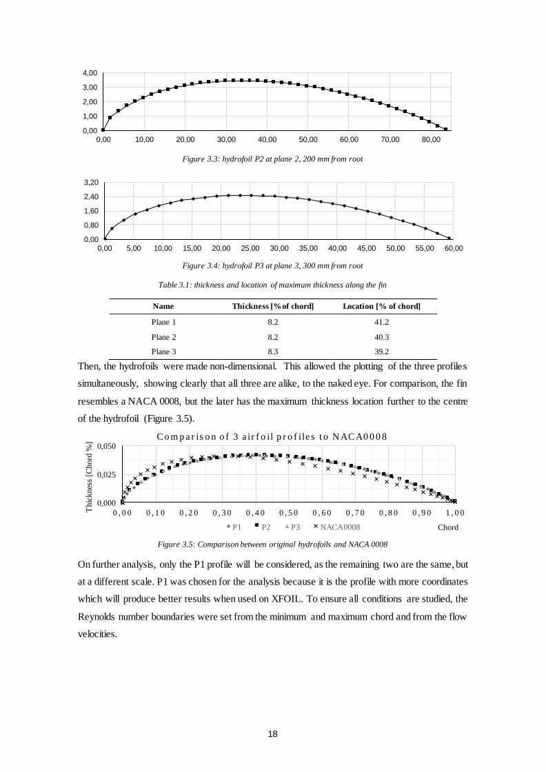
After, the sets of coordinates would be treated and plotted, like in Figure 3.2 to Figure 3.4. At this
point, only half of the profile is plotted, as the hydrofoil is symmetric.
Further investigation revealed that the fin almost has a constant profile in all its extent, aside from
the breadth reduction, like explicit on Figure 3.5. This change in maximum thickness and its
position is unneglectable.
Figure 3.2: hydrofoil P1 at plane 1, 100 mm from root
0,00
1,00
2,00
3,00
4,00
5,00
0,00 10,00 20,00 30,00 40,00 50,00 60,00 70,00 80,00 90,00 100,00
18
Figure 3.3: hydrofoil P2 at plane 2, 200 mm from root
Figure 3.4: hydrofoil P3 at plane 3, 300 mm from root
Table 3.1: thickness and location of maximum thickness along the fin
Name Thickness [% of chord] Location [% of chord]
Plane 1 8.2 41.2
Plane 2 8.2 40.3
Plane 3 8.3 39.2
Then, the hydrofoils were made non-dimensional. This allowed the plotting of the three profiles
simultaneously, showing clearly that all three are alike, to the naked eye. For comparison, the fin
resembles a NACA 0008, but the later has the maximum thickness location further to the centre
of the hydrofoil (Figure 3.5).
Figure 3.5: Comparison between original hydrofoils and NACA 0008
On further analysis, only the P1 profile will be considered, as the remaining two are the same, but
at a different scale. P1 was chosen for the analysis because it is the profile with more coordinates
which will produce better results when used on XFOIL. To ensure all conditions are studied, the
Reynolds number boundaries were set from the minimum and maximum chord and from the flow
velocities.
0,00
1,00
2,00
3,00
4,00
0,00 10,00 20,00 30,00 40,00 50,00 60,00 70,00 80,00
0,00
0,80
1,60
2,40
3,20
0,00 5,00 10,00 15,00 20,00 25,00 30,00 35,00 40,00 45,00 50,00 55,00 60,00
0,000
0,025
0,050
0 , 0 0 0 , 1 0 0 , 2 0 0 , 3 0 0 , 4 0 0 , 5 0 0 , 6 0 0 , 7 0 0 , 8 0 0 , 9 0 1 , 0 0Thic
knes
s [C
hord
%]
Chord
Co m p a r is o n o f 3 a ir f o il p r o f ile s t o N ACA0 0 0 8
P1 P2 P3 NACA0008

19
3.3.1 Initial Stage
With the non-dimensional hydrofoil ready, the coordinates’ file was introduced on XFOIL. Some
runs were made to feel how the software would work on the coordinates. The tests considered the
coordinates in Figure 3.2.
A standard procedure to improve the results, the number of panels of the hydrofoil was set to 160.
The viscosity operation was toggled on, and the Reynolds number was set to 0.50 x10⁶, with a
maximum of 200 iterations to run. In Analysis chapter, the typical routine used is explained.
For an angle of attack of 0 degrees, the pressure coefficient distribution is shown below (Figure
3.6).
The red line represents the pressure side and the blue line the suction side. On this chapter Cp
distribution Figures, the red and blue lines are overlapping since all Figures represent 0° AoA and
symmetric profiles. The dashed line is representing the inviscid pressure distribution.
Figure 3.6: Pressure coefficient distribution from p1
It is especially distinguishable an increase in the pressure just after the leading edge on Figure
3.6. Presumably, it is caused by a concavity, present along all the hydrofoil, that induces a contrary
pressure gradient.
This feature is incorrect and is a possible result from the SFWB scanning process.
To mitigate the pressure coefficient irregularity, several fairing techniques where sought. First,
several splines where adapted to the curvature. This adaptation was carried out using spreadsheet
functionalities and formulas, but the results were not satisfactory. The second attempt consisted
in reshaping manually the coordinates, as for adding coordinates or simply shifting them.
This aimed at a smoother transition between panels, later, on XFOIL, as the angle between panels
was smaller. The adaptation for the first profile is shown in Figure 3.7.

20
Figure 3.7: Comparison between original coordinates from SFWB and the faired hydrofoil
Each new change was then experimented on XFOIL until the pressure distribution was to
resemble a normal hydrofoil. The most important iterations are stored in .txt files, with the
following name code:
File name: pxyy.txt
[p]: plane
[x]: profile number
[yy]: iteration number
Next is presented the pressure coefficient distribution of the last iteration (number 13), from
profile P1, with coordinates found on Appendix A.1, and the NACA 0008 (Figure 3.8 and Figure
3.9). Both computations are at Re 0.46 x10⁶ and with AoA of 0°.
Figure 3.8: Pressure coefficient distribution from profile P113 at Re 0.46 x10⁶and AoA 0°
0,0000
0,0100
0,0200
0,0300
0,0400
0,0500
0,00 0,02 0,04 0,06 0,08 0,10 0,12 0,14 0,16 0,18 0,20 0,22 0,24 0,26 0,28 0,30 0,32
Adimensional airfoil, plane 3 Airfoil Fairing, plane 3

21
Figure 3.9: Pressure coefficient distribution from profile NACA 0008 at Re 0.46 x10⁶ and AoA 0°
When more results were to be extracted, for higher AoA’s, it was hard to obtain a solution, as the
program could not converge. This may mean some flow anomaly is present and will be
investigated after.
This was still no guarantee that the software was being well used and presenting valid results. As
such, a known profile, with wind tunnel processed data, was chosen. The idea was to recreate the
same conditions as the test but on XFOIL and compare the results.
If the validation proves successful, the faired geometry will be used to retrieve the flow data from
the software.
3.4 Analysis
XFOIL software shows a DOS environment, thus, all commands must be typed, and special rules
must be followed. A typical routine on XFOIL is explained below.
XFOIL c> load pxxx.txt
Loads the coordinates file
XFOIL c> pane
Increases the panel number up to 160
XFOIL c> OPER
Enters the Operation menu
OPERi c> ITER 500
Defines number of iterations
OPERi c> VISC [RE]
Toggles on the viscous effects at Reynolds number [RE]
OPERi c> p
Toggles on the polar accumulation
OPERi c> pxxx_[RE]_polar.txt

22
File name for polar saving
OPERi c> Enter
Disable dump file
OPERi c> SEQP
Plot polar during point sequence (optional)
OPERi c> A i
Specify alpha
OPERi c> CPWR pxxx_[RE]_CP0i.txt
Write Cp (x) distribution to a text file
…
OPERi c> A 16
OPERi c> CPWR pxxx_[RE]_CP16.txt
OPERi c> QUIT
Exits the program
The simulations were done between Reynolds 0.20 x10⁶ and 0.70 x10⁶, with increments of 0.05
x106. Since the tests will be done at such low Reynolds number, it is expected the presence of a
laminar separation bubble, like it is typical at such values.
Due to the nature of the hydrofoils, very rarely the routine was followed like above until the end.
Typically, the program could not converge at some point, usually around the AoA of 5 degrees.
One bypass for the problem was to increase the angle by one decimal. A smaller gap between
computations seemed to help. Another technique was to jump to 10 or 9 degrees and slowly
approach smaller angles. This may mean some anomaly is happening at some angle interval.
3.5 Case Study 2
As validation for the obtained results from XFOIL, a known profile with wind tunnel data was
processed on the program. The objective is to compare the results, from the experimental method
and the computational method.
• E387 Wind Tunnel Data
The chosen profile is an Eppler 387 foil (3.10), with a maximum thickness of 9.1 % at 31 % of
the chord. This profile has a 3.2 % camber at 44.8 %, not symmetrical like the SFWB profile
being evaluated. Still, has a close thickness and the data found is inside the Reynolds number
envelope.
Figure 3.10: Eppler 387 foil (in pink)

23
The data taken on the E387 originates from the results from NASA Langley taken in the Low-
Turbulence Pressure Tunnel (NASA LTPT) [20]. The tests collected data from several Reynolds
numbers; the Re of 0.46 x10⁶ was seen as appropriate for the study. Then, the fluid velocity
condition was recreated on XFOIL, and the results drawn are present in Figure 3.11.
For the lift and drag coefficients, it is safe to conclude that the two tests behave very similarly up
until 10 degrees. Above that, it is expected that the fluid boundary layers separate, entering a
realm of analysis in which the XFOIL program is not so precise.
As for the momentum coefficient, the results are only close up to 5 degrees. These results are
different because the pivot point where the profile is allowed to rotate is different. As standard,
XFOIL uses 1/4 of the chord.
Figure 3.11: Plots for the Cl, Cd and Cm coefficients on E387, using Nasa wind tunnel results and XFOIL results
3.6 Results Discussion
Considering the determined consistency of the results from the last chapter, it is assumed that the
program is being properly used. Likewise, this chapter considers the results taken from the profile
P113, obtained with XFOIL.
These results comprehend the data observed on XFOIL software, for the Reynolds numbers
between 0.20 x10⁶ to 0.70 x10⁶. The angle of attack ranges from 0° to 16° (in some cases to 15°
due to difficulties in convergence).
The pressure coefficient distribution (example in Figure 3.8), plotted to represent the non-
dimensional pressure on the surface, shows as expected, a maximum value at the nose of the
profile at zero degrees. If the flow was inviscid, that value would also be of one at trailing edge.
As the angle increases, different values of pressure coefficient are plotted for the upper surface
and lower foil surface. As commonly known, at positive AoA and symmetric aerofoils, the
0
0,2
0,4
0,6
0,8
1
1,2
1,4
1,6
-5 0 5 10 15Cl
AoA [°]
Cl, Re 4.6E5
XFoil
NASA
0
0,01
0,02
0,03
0,04
0,05
0,06
0,07
0,08
-5 0 5 10 15Cd
AoA [°]
Cd, Re 4.6E5
XFoil
NASA
-0,09
-0,08
-0,07
-0,06
-0,05
-0,04
-0,03
-0,02
-0,01
0
-5 0 5 10 15
Cm
AoA [°]
Cm, Re 4.6E5
XFoil
NASA

24
pressure is negative on the upper surface and positive on the lower surface. This effect is broadly
used to achieve lift on aeroplanes, as the wings are oriented initially on positive AoA’s. To make
the reading of the plots more intuitive, the scale has been reversed, being presented the negative
values “above zero”. Still, regarding this distribution, it was noticeable a smoother slope very
close to the tip of the hydrofoil, on the upper side. This shows that the original Cp was to follow
a certain degree of degradation, but something unexpected provoked a more severe increase in
pressure, which hints for a recirculation bubble.
The lift coefficient presents, as expected for a symmetric foil, a value of zero at AoA 0°. It shows
a linear behaviour generally until 6°; after that, it enters the stall (loses sustentation). Around 9°,
the aerofoil seems to regain lift, increasing exponentially. For the first part, on the linear
behaviour, the Cl reaches around 0.65; on the second half of the lift coefficient distribution, the
value may go until 0.72. These coefficients may be converted into forces later.
Regarding the drag coefficient curve, it is starting close to zero at AoA 0°. This is where the drag
is minimum, as the profile is in line with the flow. It is seen to increase as the angle of attack
increases, parallel to the growth of the exposed area, in the way of the flow lines. The minimum
observed value is of 0.0049, and the maximum of 0.203.
The moment coefficient, or pitching moment, is zero when no pitch is observed, congruent with
the expected behaviour. From 0° to 5°, the moment is negative, thus applying a momentum that
makes the nose of the foil point to the ground. From 5° to 10°, the moment is positive, forcing the
leading edge up. After, the momentum turns negative once more. This fits the behaviour watched
on the lift coefficient: as the momentum is created by the aerodynamic force shifting (like
mentioned before, composed by lift and drag force components).
Figure 3.12: Plots for the Cl, Cd and Cm coefficients and transition coordinates on P113, XFOIL results
Tests refer to the trial at Re 6.0x10⁵. The duality of results is achieved by solving first from small to large AoA’s,
and after from higher to smaller AoA’s.
0,00
0,10
0,20
0,30
0,40
0,50
0,60
0,70
0,80
0 4 8 12 16
Cl
AoA [°]
Cl
Cl'
0,00
0,02
0,04
0,06
0,08
0,10
0,12
0,14
0,16
0,18
0 4 8 12 16
Cd
AoA [°]
Cd
CD'
-0,03
-0,02
-0,01
0,00
0,01
0,02
0,03
0 4 8 12 16
Cm
AoA [°]
Cm
CM'

25
The analysis of the transition points of the flow, on both sides of the foil, reveals that on the lower
surface, the flow adheres practically until the trailing edge, to the AoA full interval. On the upper
surface, the flow stays laminar until 97 % of the chord at 0°, then around 2°, the separation point
shifts abruptly to the leading edge, around 4 % of the chord. This value decreases until it can be
accepted it separates on the leading edge itself.
Aside from these results, it is important to point out that some trials were made starting at angles
such as 14°, progressing to lower angles. New and different values for the coefficients were
observed, adding the previously obtained results. This is seen in Figure 3.12, where Cl, Cd and Cm
are plotted.
This leads to the conclusion that the software is finding multiple solutions for the same problem.
As such, it is safe to assume that some anomaly is occurring, which may also help explain why
the transition point changes abruptly after a given angle. Plus, would explain the difficulty in
achieving convergence on the results, as multiple solutions seem to be possible.
In sum, transition on the upper surface of the foil is to be expected, like recurrent for the low Re.
Some recirculation phenomena seem to be occurring and shall be explored sequentially in the
next chapter, where a more powerful CFD tool is to be used.

26

27
Chapter 4
Mesh, Turbulence and Transition Model
The following case study comprehends the use of the control aerofoil to verify which are the most
appropriate conditions to run the fin profile. In that matter, the choice of software, as well as the
mesh and physics models, are important to capture accurately and realistically the flow around
the profile. The Reynolds number is the same as previously used on case study 1.
4.1 CFD Software Selection
Similarly, to what was done before, the software to be used was chosen from an array of possible
choices. The main characteristics needed concern aspects such as the physical models, the
simplicity and ease of use, and the ability to obtain the desired results (lift, drag, pressure
coefficients, etc.).
There are some programs available on the market: some are open source and free, but lack
interface; others require an active license and server constant connection and others yet, can group
many modalities, like mesh generation, flow or multiphysics simulations and so on.
Ansys Fluent [21] program has the capacity to develop many physical models, from laminar to
turbulent, but lacks some of the new, cutting-edge transition models. It does offer interesting wall
treatments. The advantage is that it conciliates structural mechanics and fluid mechanics
disciplines, which can be used later to perform the fluid-structure interaction.
Star-CCM+ [22] also performs such analysis. This software is best known for its ease in use, as
well as a vast portfolio of models and parameters that may be tuned, in the fluid analysis. It also
has a robust meshing system, can read macro files and create geometries. It is vastly used at master
thesis with a CFD approach.
Finally, OpenFOAM [23] is probably the most well-known of the listed, but also the most
complex to operate. It is a fully open source software with constant updates, performs meshing,
can solve complex flow analysis, such as turbulence, heat transfer, chemical reactions or even
electromagnetics. Due to being free software, it has a large user base. That is a positive aspect of

28
having in mind if operating with OpenFOAM, as no GUI interface is available yet and much
experience is needed to obtain results.
The used software will be Star-CCM+, due to its availability and support at the Laboratory of
Fluid Simulation in Energy and Fluids (LASEF), at the Instituto Superior Técnico (IST).
4.2 Star-CCM+ Aerodynamic Models
The first step in solving the problem would have to be the physics’ model selection. Different
models need different mesh parameters, as explained below. From the low Reynolds numbers
used on this investigation, it is safe to assume that the laminar boundary layer is very unstable
and will separate at some point along the wall. As separation occurs, the flow will have a transient
state and a turbulent state further downstream. If the turbulent flow reattaches, there will be a
separation bubble between the separation zone and reattachment. The Re and the shape of the foil
influence the length of this bubble, which can be classified of short or long, the last known to be
formed at Reynolds number above 5 x 10⁵ [24]. This means that the separation bubble will have,
eventually, different lengths along the fin.
Thus, the models should contemplate transition. A brief explanation of the turbulence models
employed follows:
4.2.1 SST k – ω Turbulence Model
The k – ω SST turbulence model, developed by Menter, is a combination of two well-known
models: the k – ε and the k – ω. The k – ε, developed by Jones and Launder is a good predictor in
fully turbulent flows where the effects of molecular viscosity are neglectable. It is usually used
best on high Re numbers. On the other side, the k – ω, by Wilcox, performs best at wall integration
and is a good predictor for flow separation [25]. This way, by changing the ε to kω on the k – ε
equation, the two models blend near-wall effects, and outer layer effects are captured, resulting
in a versatile model:
𝜕
𝜕𝑡(𝜌𝑘)+
𝜕
𝜕𝑥𝑖(𝜌𝑘𝑢𝑖) =
𝜕
𝜕𝑥𝑗(Γ𝑘
𝜕𝑘
𝜕𝑥𝑗)+ 𝐺𝑘− 𝑌𝑘+𝑆𝑘 (4.10)
𝜕
𝜕𝑡(𝜌𝜔) +
𝜕
𝜕𝑥𝑗(𝜌𝜔𝑢𝑗) =
𝜕
𝜕𝑥𝑗(Γ𝜔
𝜕𝜔
𝜕𝑥𝑗)+ 𝐺𝜔 − 𝑌𝜔 +𝐷𝜔 + 𝑆𝜔 (4.11)
On the above, the diffusivity is present in Γω and Γk. The turbulent kinetic energy generation and
specific dissipation rate are given by the variables Gω and Gk. The Yω and Yk are representing the
dissipation and the Sk and Sω the source terms. Finally, to blend the two models, the variable Dω
is the extra cross diffusion with the formula:

29
𝐷𝜔 = 2(1 −𝐹1 )+ 𝜌𝜎𝜔, 21
𝜔
𝜕𝑘
𝜕𝑥𝑗
𝜕𝜔
𝜕𝑥𝑗 (4.12)
4.2.2 γ – Reθ Transition Model
Once it is to be determined if the flow is fully turbulent or if the transition occurs somewhere
along the surface, the present model is also in scope. The γ – Reθ was developed specially for
transition flows and combines the SST K-ω with intermittency γ and a transition triggered by a
specific local Re. In this case, Reθ symbolises the critical Re number at which the intermittency
will start [26].
This phenomenon is given by [27]
𝜕(𝜌𝛾)
𝜕𝑡+𝜕𝜌𝑈𝑗𝛾
𝜕𝑥𝑗= 𝑃𝑥𝛾1 −𝐸𝛾1 +𝑃𝑥𝛾2 −𝐸𝛾2 +
𝜕
𝜕𝑥𝑗[(𝜇 +
𝜇𝑡𝜎𝛾)𝜕𝛾
𝜕𝑥𝑗] (4.13)
𝜕(𝜌𝑅𝑒̅𝜃𝑡)
𝜕𝑡+𝜕(𝜌𝑈𝑗𝑅𝑒̅𝜃𝑡)
𝜕𝑥𝑗= 𝑃𝜃𝑡 +
𝜕
𝜕𝑥𝑗[𝜎𝜃𝑡(𝜇 +𝜇𝑡)
𝜕𝑅𝑒̅𝜃𝑡𝜕𝑥𝑗
] (4.14)
As for coupling the transition on the SST K-ω, the K- equation is modified as:
𝜕
𝜕𝑡(𝜌𝑘)+
𝜕
𝜕𝑥𝑖(𝜌𝑘𝑢𝑖) =
𝜕
𝜕𝑥𝑗(Γ𝑘
𝜕𝑘
𝜕𝑥𝑗) +𝐺𝑘
∗− 𝑌𝑘∗+ 𝑆𝑘, 𝐺𝑘
∗ = 𝛾𝑒𝑓𝑓�̅�𝑘 𝑎𝑛𝑑
𝑌𝑘∗ = min (max(𝛾𝑒𝑓𝑓0.1) ,1.0)𝑌𝑘
(4.15)
However, attention must be given to wall Y+ modelling: if the mesh does not allow Y+ ≤ 1, the
viscous sublayer effect will not be captured and the transition models are working above will not
be properly modelled.
4.3 Mesh Characteristics
For the models to work accordingly to the desired, the mesh definition was an iterative process.
If the grid created was too coarse, the boundary layer phenomenon would not be captured, but a
mesh too much refined takes a long time to be computed.
In total, polyhedral elements and prism layers are the building blocks, with the added feature of
surface remesher, available on Star-CCM+. For the boundary between hydrofoil and domain, the
prism layer was used, as traditional. This is a layer that tends to follow the surface of the boundary,
and, for modelling the boundary layer, proves efficient.
In an attempt to obtain shorter times for the mesh creation, the domain was divided into areas,
which would allow a tune of the mesh characteristics inside each. This way, besides the main
three-dimensional domain there are smaller volumes: V1.0, V2.0 and V3.0. The volume V1.0
contains the hydrofoil and the two other volumes. The volume V2.0 contains again the aerofoil
and V3.0, but much closer to the walls. Its purpose is to refine only the cells at the surface. Finally,
V3.0 is composed by V3.1, refining the leading edge and V3.2 the trailing edge. The chord length
defined is 100 mm, which is equivalent to the length at the root of the SFWB. The three volumes

30
and domain dimensions are in table 4.1. The thickness is, as common practice, 5% of the chord
length.
Table 4.1: domain and control volumes’ dimensions
Name Width [chord lengths] Height [chord lengths]
Domain 20 15
V1.0 3 1
V2.0 1.2 0.2
V3.1 0.013 0.04
V3.2 0.025 0.01
These volumes were used on case study 3 and 4, except for V3.2 on case 3, which did not need
refinement. Associated to them are the element sizes. The idea was to have significant elements
near the inlets and outlet and a very fine mesh around the profile and after the exit slab. So, the
main domain has elements that can be five times bigger than the hydrofoil chord, with a rate ruling
the cell contraction until the boundaries of the control volumes. Table 4.2 sums the input
parameters for the mesh creation and Figure 4.1 depicts the final result. Except the values stated,
all the remaining values were left as standard. All the values are in absolute dimension.
Table 4.2: domain and control volumes’ mesh parameters
Name Mesh Continuum
Base Size [m] 0.5
Nº of Prism Layers 30
Prism Layer Stretching 1.15
Prism Layer Thickness [m] 0.005
Surface Growth Rate 1.08
Surface Absolute Minimum Size [m] 2.0E-4
Surface Target Size [m] 1.0
Control Volumes: V1.0 V2.0 V3.0
Polyhedral base size [m] 0.001 2.8E-4 3.2E-5
Nº of Prism Layers - 30 -
Prism Layer Stretching - 1.15 -
Prism Layer Thickness [m] - 0.0035 -

31
Figure 4. 1: Mesh definition
One of the main challenges was to develop a mesh that would lay around both aerofoils smoothly.
The leading edge on the SFWB was the trickiest zone: because the fin is very slim, the curvature
would be truncated in faces, decreasing the detail degree. Also, a very thick prism layer, with
constant aspect ratio produced large cells at the tip, which is not favourable for the analysis. So,
the solution was to divide the control volumes like explained above, with a smaller prism layer
thickness and small cell dimension, assuring a good fit around the geometry on both cases.
4.4 Case Study 3
Much like case study 1, the present case aims to verify the most realistic conditions to perform
the analysis. As stated, the E387 profile will be studied, operating the mesh and models described
previously. The results to be shown are the result of several iterations and the most interesting to
be presented.
The conditions of the precedent tests were simulated. As the hydrofoil is now a finite and defined
solid, the inlet condition, the Reynolds number, had to be accordingly translated into velocity.
So, the velocity to be used in the test is given by:

32
𝑅𝑒 =𝑈𝑐
𝜐⟺ 𝑈 =
𝜐 ∙ 𝑅𝑒
𝑐⟺ 𝑈 =
1.05𝐸 − 06 ∙ 4.6𝐸5
0.1⟺ 4.83 𝑚 ∙ 𝑠−1 (4.16)
The different angles of attack will be obtained by rotating the virtual laboratory referential, so all
the conditions are maintained through the analysis. The fluid to be simulated is water, with
dynamic viscosity from table 2.1.
The simulation setup consisted of applying the next models: two-dimensional, segregated flow,
liquid (at constant density), turbulent, k – ω SST turbulence model and low Y+ wall treatment.
Two simulations for each angle are performed: with transition model γ – Reθ, and without
transition model. The objective is to determine which provides the closest results to the
experimental data.
At the inlet, the turbulence intensity and turbulent length scale were, as good practice demands,
of 0.1% and 10% of the hydrofoil thickness, respectively.
When simulating solely with the k – ω SST turbulence model, typically the residuals converge
efficiently. That is why it is much used when the flow is known to be turbulent from the start. In
some cases, the residuals would stall at a value above 105 because k – ω SST failed to find the
transition point on the surface, an understandable feature for a turbulence model. To bypass this
problem, two ways where used: the first one consists in changing the inlet velocity for one or two
iterations length. This would disturb the flow and help the model find the transition point. Another
way and the one that proved most effective was changing the relaxation factor. The values applied
are between 0.3 and 0.7, always lower than the predefined.
For the γ – Reθ model, the residuals did not converge using a steady state solver. To obtain valid
values, the implicitly unsteady solver would be toggled on. Then, by changing the time step time
and the number of inner iterations, the residuals where made drop by 2 orders. The solution found
is stationary (oscillations of force coefficients of 10-5 decimal). Again, when needed, the
relaxation factor is changed between the previous interval. The wall Y+ was kept under 1 in most
of the foil surface.
Using the data compiled, the results from both models were then compared to the wind-tunnel
and XFOIL points. On Figure 4.2 are presented the lift and drag coefficients from the four
different sources. For the lift coefficient, both models provide satisfactory results. The k – ω SST
model shows a slightly higher value for the peak of the curve, with a maximum error of 6 %. The
γ – Reθ models this quantity with more accuracy and more times, meaning the deviation from the
wind-tunnel data is more often with errors below 2 %. That is also true for the drag coefficient,
until around 8 degrees where the error is below 9 %. The k – ω SST model has an overall less
good performance, with errors reaching 52%.

33
(a) Cl versus AoA, Re 4.6 x10⁵
(b) Cd versus AoA, Re 4.6 x10⁵
Figure 4.2: E387 lift and drag coefficients results from STAR-CCM+, XFOIL and Wind-tunnel experiments
The results from the k – ω SST model without the transition add-on may be explained due to the
nature of the model itself. As summarised in 4.2.1 SST k – ω Turbulence Model, the model
developed by Menter is specific for when turbulence is known to be present and develops near
the leading edge. That does not seem to be the case in this simulation since the transition model
depicts a laminar behaviour until some extent on the profile surface. So, if the turbulence model
determines that transition is occurring near the leading edge, the drag component from the
turbulent kinetic energy, which extends at full length on the suction side, may add the extra
percentage that is seen at the results. That turbulent behaviour will be seen next.
Figure 4.3 represents the intermittency factor and Figure 4.4 and Figure 4.5 the turbulent kinetic
energy, for the E387 aerofoil at an angle of attack of 4°. The intermittency factor shows the
probability at a given time and space of the flow to be turbulent or laminar, where red represents
turbulent flow and blue laminar flow. When the flow closes to the hydrofoil wall, the
intermittency near the wall is zero: the flow does not have the probability to be turbulent.
However, that changes around half of the hydrofoil, where the flow will have a turbulent fashion
(intermittency of 1). The negative velocity in i direction is also plotted in grey scale but is so small
in the pictures it becomes hard to spot. Despite that, this may be the best indicator of a laminar
separation bubble (LSB), because, like covered on 2.7 Boundary Layer, due to the adverse
pressure gradient, the flow will tend to circulate backwards near the wall and again on the initial
flow direction when it touches the upper flow layers. The intermittency value of near 0 at that
area credits this theory, as also anticipated in Case Study 1. The length of the LSB is around 16%
0
0,2
0,4
0,6
0,8
1
1,2
1,4
1,6
-5 0 5 10 15 20
Cl
AoA [°]
XFoil
NASA
γ – Reθ
k – ω SST
0
0,02
0,04
0,06
0,08
-5 0 5 10 15 20C
d
AoA [°]
XFoil
NASA
γ – Reθ
k – ω SST

34
of the chord, categorising it as a short bubble [24], and its thickness of 1 % (double of the value
measured since the vector only shows the backward circulation). Finally, Figure 4.4 verifies the
above, where the turbulent kinetic energy has a peak about the end of the LSB, signalling the
reattachment of the flow to the turbulent boundary layer. These effects are observed throughout
different AoA’s.
On Figure 4.5 is proved that the k – ω SST model predicts the flow separation sooner than the
transition model. No LSB is present on the results from this model.
Figure 4.3: Intermittency for the aerofoil E387, AoA 4°, k – ω SST γ – Reθ
Figure 4.4: Turbulent Kinetic Energy for the aerofoil E387, AoA 4°, k – ω SST γ – Reθ
Figure 4.5: Turbulent Kinetic Energy for the aerofoil E387, AoA 4°, k – ω SST

35
Using the visual tools from Star-CCM+, an estimate of the transition location is presented in
Figure 4.6. No model gives an exact location for this phenomenon, so the measure is done by
verifying the peak in turbulent kinetic energy, near the hydrofoil wall. On this analysis, only the
results from the γ – Reθ model are used. Any measurements from the k – ω SST model would not
contemplate the transition effects and flow reattachment. The results are compared to the XFOIL
data.
Reading the Figure 4.6, Star-CCM+ predicts a later transition on the suction side, and an earlier
transition on the pressure side, comparatively to the XFOIL results. Some factors may be the
underlying cause of these inconsistencies. For example, XFOIL predicts transition but not
recirculation, as of its nature. It has been seen that recirculation is occurring on this case. Also,
on XFOIL the geometry was obtained using the coordinates from the website Airfoil Tools. These
coordinates would prove insufficient to create panels, panels that would model the surface. Thus,
the command PANE was used to multiply the number of panels. This may have deformed the
geometry slightly, resulting on different values from Star-CCM+. For the later, the approach was
different, as it begun with the same coordinates, but a special spline was fitted using the tools
available on Rhinoceros 3-D software. This created a smooth surface, with no vertices subsequent
from planes. Even the initial flow configurations on XFOIL, which were left as original, may
have influence. As for Star-CCM+, the values regarding freestream turbulence intensity and
turbulent length scale may not be the most appropriate or alter the final results. The mesh may
also cause perturbations on the transition point if it is not adequately refined. However, as wall
Y+ factor was kept in consideration along with the simulations, and compels the mesh to be
conveniently refined, it is unlikely to be the problem.
Finally, the pressure distribution is plotted for the AoA of 0° (Figure 4.7). The results from Star-
CCM+ follow the same fashion as the XFOIL data, although less accurately on the suction side.
The pressure coefficient seems higher on the suction side, and the pressure leap, due to the
separation, also comes slightly after. On the wind-tunnel results, possibly due to the low amount
of sample points, the pressure has the same magnitude but much less definition on the leading
edge and at the separation point.
Figure 4.6: Transition curves for E387, XFOIL vs k – ω SST + γ – Reθ
0%
20%
40%
60%
80%
100%
-2 0 2 4 6 8 10 12 14
% c
AoA [°]
Xfoil suction side
Xfoil pressure side
γ – Reθ suction side
γ – Reθ pressure side

36
Figure 4.7: E387 pressure distribution, AoA 0°, k – ω SST γ – Reθ
4.5 Validation Conclusions
This chapter ends with a preview of the necessary models and instructions for the following
chapters. The main two ingredients: the mesh parameters and the models and methodology on
how to operate these models was verified here.
For the 2-D analysis, the mesh parameters will be the ones used in this chapter. The objective is
to recreate as faithfully the conditions in all simulations.
The two models under the scope, the k – ω SST and its add-on γ – Reθ model for transition were
compared. The k – ω SST performs well for lift determination but fails for drag estimation. It is
also uncapable of correctly estimating the transition point. The reasons to first consider this model
was for the fact that the simulation residuals tend to converge fast, saving time and because the
simulation could be turbulent since start.
On the other side, adding the transition model, the lift and drag coefficients are correctly
estimated, and provide close values to the wind-tunnel tests. The transition can be estimated,
although, without wind-tunnel data, it is impossible to say which of the tests performed (Star-
CCM+ and XFOIL), is closer to reality.
That being said, the γ – Reθ will be the only model to be applied on the next stages, as it is expected
to estimate the lift and drag coefficients, transition and pressure closer to real experiments.
-1
-0,5
0
0,5
1
1,5
0 0,1 0,2 0,3 0,4 0,5 0,6 0,7 0,8 0,9 1
Cp
Chord Length
Xfoil
Star ccm+
NASA

37
Chapter 5
SFWB Profile Performance
Following the validation done in Chapter 4, the present chapter will explore the behaviour of the
fin profile using the previous conditions. The results are compared to the estimations made in
Chapter 3, for case study 1.
5.1 Case Study 4: SFWB Results
Using the aerofoil from case study 1 after the repair, the simulation was replicated like Chapter
4: Mesh, Turbulence and Transition. The same mesh parameters and physics’ models where used.
For the velocity, only three flow speeds are employed and represent the expected low, mean and
top speeds the fin will experience. This way, only simulations at the Re numbers of 2.5 x10⁵,
5.0 x10⁵ and 7.5 x10⁵ (respectively 2.100, 5.250 and 7.875 m/s), where performed. The fin chord
is of 100 mm (corresponding to the length at the root).
Regarding CFD simulation nature, the P113 profile behaves like the E387: no convergence is
found when using the steady state solver. At the beginning of simulations, especially for larger
angles of attack, vortexes could be seen before the simulation converged. When the residuals
drop, this instability will disappear. One of the possibilities is for it to be Von Kármán vortex
street, but, as simulations converge, it ceases to produce vortexes. Another option is Kelvin
Helmholtz instability, which is characterised by a velocity difference, in this case, between the
fluid and the fin interface. The velocity shear induces the formation of what looks like curls, and
the initial, larger ones dissipate when the velocity stabilises. Near the wall may be occurring
instability, which is so small it is hardly captured. This surface tension does not seem to have a
significant interference in the lift, drag and pressure distribution. For example, for the Re of 7.5
x105, it is clear to see at 8 degrees (around when the foil stalls), that the variation of pressure and
lift is approximately 10-3 (Figure 5.1, Figure 5.2 and Figure 5.3). This way, and since the first
seconds into the simulation the field is not physical (breaks continuity laws), an unsteady solver
is used, that in the end depicts a steady solution.

38
Figure 5.1: Lift coefficient monitor, Re 7.5 x10⁵, 8° AoA
Figure 5.2: Variance of Pressure for the complete simulation, Re 7.5 x10⁵, 8° AoA
Figure 5.3: Q-Criterion for converged solution, Re 7.5 x10⁵, 8° AoA
As Figure 5.1 shows, the lift coefficient tends to stabilise to a number with 5 decimals after 2
seconds. At this stage, the residuals are fully converged, leading to the belief that the solution is

39
found. In Figure 5.2, the mean variance of the pressure along the profile is depicted. As expected,
the variance is more significant near the leading edge, due to the fluctuation of the fluid and the
point of separation. Also, of relevant value is the variance near the trailing edge, expected once
turbulence will occur as the fluid leaves the pressure side of the foil. Parallelly, to help visualise
the shape of the turbulent field, the Q-Criterion is shown in Figure 5.3. This scalar displays the
LSB clearly at around 50 % of the hydrofoil, followed by a reattachment zone, and then evolving
to turbulence.
Concerning transition, the results were taken in the same way as Chapter 4. The wall Y+ was
verified to be below 1, at the mesh generation stage, so case study 3 and 4 had to be done almost
simultaneously to obtain a mesh that fitted both. Figure 5.4 below represents the transition curves
from XFOIL and-Star CCM+, for a Reynolds number of 5 x10⁵. The behaviour in both cases is
alike, with Star-CCM+ predicting separation on the suction side somewhat earlier. That may be
due to the way the measurement was done since no function with the used models provides the
exact place for the transition.
Figure 5.4: Transition curves for P113, XFOIL vs k – ω SST + γ – Reθ., Re: 5 x10⁵
This transition behaviour is complemented with the formation of laminar separation bubbles.
Taking the example of the simulations for Re 5 x10⁵, it is seen the formation of twin bubbles, on
suction and pressure side, at the trailing edge. This fits with the transition prediction results, which
show transition at about 97 % (see Figure 5.5). As the angle of attack increases, the LSB shifts to
the leading edge. Depending on the direction of the flow, the pressure side will always tend to
-0,10
0,10
0,30
0,50
0,70
0,90
1,10
0 4 8 12 16
Xtr
AoA [°]
XFOIL suction side
XFOIL Pressure side
k – ω SST γ – Reθ suction side
k – ω SST γ – Reθ pressure side

40
have a full laminar flow around it. Three bubbles appear in Figure 5.6: one at the trailing edge on
the pressure side, and two on the leading edge. The first one, on a), shows the flow is recirculating
at the tip, but the outer layers of the flow remain laminar, as no turbulence is identified. For the
leading edge, on b), the bubble seen at the pressure side is not an actual bubble but only a
characteristic of the flow hitting the wall, stagnating and accelerating around it, on -i direction
(Figure 5.7).
Figure 5.5: Turbulent Kinetic Energy for the hydrofoil P113, AoA 0°., Re: 5 x10⁵, γ – Reθ
(a) Recirculation bubble at the trailing edge
(b) Recirculation bubble at the leading edge plus stagnation point
Figure 5.6: Turbulent Kinetic Energy for the hydrofoil P113, AoA 4°., Re: 5 x10⁵, γ – Reθ

41
(a) Trailing edge recirculation bubble
(b) Recirculation bubble at the leading edge plus stagnation point
Figure 5.7: Velocity vector line display for the hydrofoil P113, AoA 4°., Re: 5 x10⁵, γ – Reθ
(a) Cl versus AoA and LSB length
(b) Cd versus AoA
Figure 5.8: Lift coefficient and LSB length in chord percentage for AoA spectrum, Re: 5 x10⁵, γ – Reθ
The actual laminar separation bubble is at the suction side and, at 4 degrees, measures about 4 %
of the chord length. The size of the LSB increases consistently with the progression of the AoA’s
and proves essential for the stall of the profile as shown in Figure 5.8. This shows a direct
0%
20%
40%
60%
80%
100%
0,00
0,20
0,40
0,60
0,80
0 4 8 12 16
Cl
AoA [°]
Xfoil
γ – Reθ
LSB lenght %
0,00
0,05
0,10
0,15
0,20
0,25
0 4 8 12 16
Cd
AoA [°]
Xfoil
γ – Reθ

42
dependence of the size of the bubble and the moment where the profile starts to lose lift. As seen,
around 8 degrees, the size of the LSB is about 30 %. The lift coefficient drops at this point, as
stall sets, this behaviour predicted at the experiments from Lissaman P. [28]. Before, as the LSB
starts to grow, the slope of the Cl starts to drop, as expected.
The values for the lift and drag coefficient, on the previous Figure 5.8, much like case study 3, on
Figure 4.2, show how the XFOIL and Star-CCM+ provide different results. For the lift coefficient,
the obtained values are overall higher on the XFOIL simulation than the results provided on the
Star-CCM+. The curve is also smoother, but that may be due to the number of samples. For the
Cd, the situation is reversed: Star-CCM+ detects less drag than its counterpart. This may be due
to the number of cells on Star versus the length of the panels on XFOIL. The orientation of the
poor panelling distribution on XFOIL may be contributing to the increase of area in the way of
the flow, making this coefficient rise. All these results are expected since XFOIL has limitations
on transition.
Because on the first seconds into the simulations, the foil induces a significant disturbance in the
flow, a detailed analysis of the pressure has been done. This comprehends the analysis of the
values’ flotation, on each cell around the hydrofoil wall, and the calculation of the mean value
from a set of measurements. The results from this study show that, after the residuals are
converged, the pressure flotation is less than 1 Pa, which may be neglected comparing to the value
order, 10- 3. This way, a graph comparing the Star-CCM+ and XFOIL results is plotted, showing
the pressure around the foil (Figure 5.9). The most visible distinctions are on the leading edge on
the suction side. Although the module value is very similar at the tip, the pressure distribution
after behaves distinctively. There is a pressure rise after the tip, with a small plateau, and after
approximately 10 % of the chord, the pressure registered on Star-CCM+ is higher than the one
delivered by XFOIL. The first difference may be explained by the nature of the transition model,
which may be giving fine details and simulating the laminar separation bubble, hence the pressure
rises, or could as well be the increase of cells in the mesh compared to the number of panels for
the XFOIL. As for the second part, the reattachment of the turbulent boundary layer may be
influencing the results, which would not be captured on XFOIL. At the pressure side, since no
bubbles or other transition singularities are expected, the results are relatively the same.
Finally, interestingly, still, for 4 degrees simulation, there seems to be a boundary layer where the
flow as equal chance to be laminar or turbulent (in Figure 5.10, as seen with the intermittency
scalar). This boundary layer forms above the viscous layer and the turbulent reattached boundary
layer, caused by the leading-edge separation bubble and holds until the end of the profile. This
favours the idea of an LSB, with linear flow above it.

43
Figure 5.9: Pressure Coefficient for the hydrofoil P113, AoA 4°, γ – Reθ
Figure 5.10: Intermittency for the hydrofoil P113, AoA 4°, γ – Reθ
5.2 Mesh Convergence Study
In order to prepare the next chapter regarding the 3-D fin study, a mesh convergence study was
performed. This study will provide the mesh size that inputs a 5 % to 10 % error in the results.
The characteristics are the 5 x10⁵ Re and 8 degrees of angle of attack. The lift and drag coefficient
will be the parameters to be analysed.
The study began with the previously used mesh and evolved to a lesser number of cells. The
parameters adjusted were the control volumes cell size. Table 5.1 compiles all the seven different
mesh sizes and respective results. All the studies complied with the wall Y+ factor smaller than 1.
Mf represents the initial mesh, and on the following numbers, the mesh becomes coarser.
-0,5
-0,4
-0,3
-0,2
-0,1
0
0,1
0,2
0,3
0,4
0,5-3
-2,5
-2
-1,5
-1
-0,5
0
0,5
1
1,5
0 0,01 0,02 0,03 0,04 0,05 0,06 0,07 0,08 0,09 0,1
Cp
Chord [m]
XFOIL
Star-CCM+
Aerofoil

44
Table 5.1: SFWB two-dimensional mesh parameters
Mf M1 M2 M3 M4 M5 M6 M7
Base Size [m] 0.5 0.5 0.5 0.5 0.5 0.5 0.5 0.5
Number of Prim Layers 30 30 30 30 30 30 30 30
P. Layer Stretching 1.15 1.15 1.15 1.15 1.15 1.15 1.15 1.15
P. Layer Thickness [m] 0.005 0.005 0.005 0.005 0.005 0.005 0.005 0.005
Surface Growth Rate 1.08 1.08 1.08 1.08 1.08 1.08 1.08 1.08
V1.0 Costume Size [m] 0.001 0.0015 0.002 0.003 0.004 0.006 0.008 0.010
V2.0 Costume Size [m] 2.8 x10⁻⁴
3.0 x10⁻⁴
3.5 x10⁻⁴
4.0 x10⁻⁴
4.5 x10⁻⁴
5.5 x10⁻⁴
7.0 x10⁻⁴
0.001
V3.0 Costume Size [m] 3.2 x10⁻⁵
3.5 x10⁻⁵
4.0 x10⁻⁵
4.5 x10⁻⁵
5.0 x10⁻⁵
8.0 x10⁻⁵
1.2 x10⁻⁴
5.0 x10⁻⁴
C l difference [%] - 0% 0% 0% 1% 1% 1% 1%
Cd difference [%] - 0% 1% 2% 2% 3% 4% 7%
Number of Cells 108224 80230 62135 48938 42212 32683 25382 17583
To decide on the best mesh to proceed with, the same physical models from the previous case
studies 3 and 4 were used. The simulations start from the implicitly unsteady state, 2nd order, and
at a time step of 0.01 and 60 iterations. This method provides quick and full convergence of the
residuals for the first 3 studies. For the remaining, the time step and the number of iterations per
time step had to be increased, being around 0.001 and 80, respectively, to obtain converged
values. This increased the computation time.
The last mesh, M7, goes out of the scope for having a difference in a drag coefficient of 7 % to
the finer mesh. It is noticeable that the drag coefficient is also the most delicate factor on the
study, perhaps because it is measured in the i direction, and this is where the number of cells is
more substantially reduced. By other words, the number of cells transversely to the foil is
significantly inferior to the number of cells longitudinally, so, increasing the cell size will make
the number of cells decrease, thus resulting on a worse result.
So, the mesh parameters to be used are the ones with a lesser number of cells but still inside the
5% error margin. M6 is a good candidate for further analysis, since the low number of cells, 23.5%
of the original value, promises to shorten the computation time.
Figure 5.11 shows how the Cl and Cd results obtained for each mesh may fluctuate around a
polynomial a 3rd and 2nd order function. The outliers where kept but should be disregarded.
It needs to be taken into account that having a less refined mesh will improve computational time
but on the other side, takes a levy in the results.

45
Figure 5.11: results for Cl and Cd for different meshes
5.3 General Conclusions
The present chapter aimed at characterising the flow around the hydrofoil. This characterisation
understood not only the usual coefficients, like lift, drag and pressure but also the intrinsic features
developed by its geometry. The work was made easier due to the previous chapter, that opened
the way for the best mesh and physical model parameters, that work fit for the required velocity
window.
There were three simulation sets, for the three velocities, despite only Re 5 x10⁵ is shown. The
remaining tests are for other ongoing investigations, that require the approximate value for the
pressure at the SFWB.
To have a better equivalence between case 4 and the previous case 3, the two meshes were
developed simultaneously. This way, the wall Y+ factor could be coordinated, and both meshes
made with parameters that would fit E387 and P113 profiles.
The best model for this case was the γ – Reθ, that was run with an implicitly unsteady solver (step
between 0.01 and 0.001), and 20 to 80 iterations per time step, depending on the velocity and
angle of attack. The presence of laminar separation bubbles is guaranteed, and these govern the
behaviour of the flow and the coefficients. The bubble increases size as the angle of attack rises
until the flow entirely separates from the suction side and only a massive recirculation bubble is
left covering all lower pressure surface.
Considerable concern was given to the pressure values, as they are the material need for another
ongoing thesis. These values would be calculated via the mean value, and the extreme values
evaluated. Once the vortex phenomena disappear, the values of pressure stabilise and assumed to
be stationary.
0,589
0,590
0,591
0,592
0,593
0,594
0,595
0,596
0,597
0,598
Cl
0,056
0,057
0,058
0,059
0,060
0,061
0,062
0,063
Cd

46

47
Chapter 6
SFWB Operation
As a final step to understand the flow behaviour, the simulations took the final step. In this chapter,
the conditions used in Chapter 5 will be summoned to create a 3-D fin simulation. Only one
velocity and angle of attack case will be investigated on this thesis, although more cases are under
study. The fin, the initial reference for the 2-D geometry that had to be fair, was not changed and
represents the piece as the maker first crafted.
6.1 Physical models and mesh considerations
Concerning the physics models, they are the same as used before. This way, there will be the k –
ω SST turbulence model with the add-on of γ – Reθ.
In what relates to the mesh, efforts were made to have a close mesh to the one used in Chapter 4
and Chapter 5.
On the previous studies, all the control volumes are rectangular, as the section was only used on
a 2-D study. For the 3-D analysis, it is essential to have in mind that the fin has different
configurations in its length. That means that, if a prismatic control volume is fitted, the distance
between its interface and the fin surface is changing in the z-direction. The cell size will be small
in areas where there is no interest in having small cells and only adds to the simulation time. That
is especially true for the V3, that has the smaller cell size. At first, the control volume V3 was
designed to cover only the leading and trailing edge, like on the 2-D simulation. To simplify that
model, the next idea was to have a fin 20 % larger to be the control volume, guaranteeing a small
mesh size along all the surface. That operation proved to be unreliable, as the number of cells
would exceed 100M and the program crash. Thus, simulations were performed using V1 and V2
with sizes on table 6.1 and configuration on Figure 6.1. V3 is not considered on this analysis.
When producing the 3-D meshes using the M6 parameters from Chapter 5.2, the M6 took around
two hours with an Intel(R)Xeon(R) CPU E5-2650 v2 @ 2.60GHz with 158 GB RAM, generating
11M cells.

48
In the subject of simulations, these start at 0 degrees of AoA and are run in a steady state for
around 100 iterations. After the solver is switched to implicitly unsteady, and the residuals made
converge. This is done by tuning the time-step and the number of inner iterations. When
convergence is attained, and without changing any previous settings, the AoA is changed. If not
needed, no further changes are made to the time step and number of inner iterations.
Table 6.1: domain and control volumes' dimensions for 3-D solution
Name Width [mm] Height [mm] Depth [mm]
Domain 2000 1500 725
V1 300 100 400
V2 120 200 400
(a) Fin
(b) V1
(c) V2
(d) Global Volume
Figure 6.1: 3-D Control Volumes

49
6.2 SWBD Three-Dimensional Aerodynamic Analysis
As stated at the beginning of this chapter, only one case, meaning one angle of attack at one
velocity regime will be under the scope. This case is at Reynolds 5.0 x10⁵ and 0° of AoA. The
remaining cases will be characterised on future work.
In what concerns the laminar separation bubble, the results from the 2-D analysis show a bubble
on both sides, near the trailing edge, covering about 18 % of the surface. For the 3-D study, the
scenario is similar, having a proportional LSB along three-quarters of the fin and covering 18%
of the chord, and a narrower bubble near the tip (Figure 6.2). This bubble fades and disappears at
the tip, while near the board surface it is inexistent, due to the boundary layer. It is expected that
the LSB will increase chordwise on the suction side while translating towards the leading edge.
These results are to be verified in future work. It will also be verified if, after 8 degrees, the bubble
bursts and all the flow become turbulent.
Also, will also be peremptory to determine the lift and drag coefficients, and values have the AoA
increases. As the results from Chapter 5 suggest, the foil should stall after 8°, typically 2 to 3
degrees after the 2-D analysis results. This will also be asserted or refuted in the future.
Figure 6.2: LSB at the Fin, Re: 5.0 x10⁵, 0° AoA
Concerning the pressure distribution, a plot was obtained for the planes captured on Chapter 3.3
(see Figure 6.3). The suction and pressure symmetric sides are overlapped and, thus, only one
curve for each section is depicted. These curves confirm the previous statement, in Chapter 3, that
similar results are found in all sections. These are only scaled and have different Re numbers.
Result wise; the curves illustrate the same particularities as the initial results from Chapter 3.3.1.
It is clear the small pressure increase near the leading edge, a characteristic of the fin foil. The
three curves have approximately the same magnitude, indicative of a constant flow velocity span
wise.
Figure 6.4 compares the pressure results from Chapter 5 and the first curve from Figure 6.3, which
are located at the same section of the fin (z =100 mm). Like previously, the most distinguishable

50
characteristics is the step on the pressure near the leading edge. Also, as the Figure now uncovers,
there are also differences on the trailing edge pressure. This may be different owed to the
adaptation from 3-D to 2-D, which mandated a treatment on the trailing edge, due to the
discretisation of the surface. When extracting the coordinates for the 2-D hydrofoil, a gap was
formed at the trailing edge, that was then closed with a semicircle. Another possibility is the mesh
size. The mesh size on the 2-D analysis is more refined than the mesh on the 3-D, the later
resultant of a mesh conversion study, and, additionally, the third control volume was not included.
Other than that, the results are coincident.
Figure 6.3: Fin Ox Pressure curves for AoA = 0°
Figure 6.4: Comparison between 2-D and 3-D results: Pressure
-4000
-2000
0
2000
4000
6000
8000
10000
12000
14000
16000
0 0,01 0,02 0,03 0,04 0,05 0,06 0,07 0,08 0,09 0,1 0,11 0,12
P [
Pa]
x [mm]
Fin Pressure curve, z=100mm
Fin Pressure curve, z=200mm
Fin Pressure curve, z=300mm
-4000
-2000
0
2000
4000
6000
8000
10000
12000
14000
-0,01 0 0,01 0,02 0,03 0,04 0,05 0,06 0,07 0,08 0,09 0,1
P [
Pa]
x [mm]
2D results: hydrofoil P113
3D results: fin section z=100 mm

51
Another interesting occurrence to verify is how the flow behaves after passing the recirculation
bubble. After the flow recirculates, in theory, it should reattach as a turbulent boundary layer.
Although in the previous chapter this phenomenon is more noticeable for higher AoA’s, it is still
included in the analysis. It is expected a small band just after the LSB and at the point where in
Figure 6.3 the pressure increases, near the trailing edge. Confronting Figure 6.5 to these
suppositions proves that they do occur, as the red band symbolises the LSB and the blue band the
turbulent kinetic energy, a signal for turbulent flow. It is also curious to notice the collar around
the fin and the plane where the fin fits the board. At this place, the mixture between the two
perpendicular flows, the one on plane xOy for the board, and the one on xOz for the fin creates a
zone of turbulence. Moving down in Z, it is seen that the TKE isosurface extinguishes, only to
reappear at the fin tip.
In Figure 6.6 it is essential to state the higher values of skin friction at the leading edge, and also
a small and thin band close to the trailing edge. This band, best visible near the fin attachment to
the board, is the line where the flow is reattaching as a turbulent boundary layer. It is also seen
higher friction values at the collar, at the same place where in Figure 6.5 is found the TKE blue
band.
In Figure 6.7 are shown the streamlines. These lines are smooth and show no signs of turbulence
or vorticity, although that is expected for the 0° AoA. For higher AoA’s will be expected the
formation of a spiral vortex at the foil tip. The blue colour on the streamlines indicates that the
flow decelerates, represented at the leading edge (the stagnated flow), and at the final half of the
fin, close to the trailing part. It is in balance with the pressure solution from Figure 6.3.
Figure 6.5: Turbulent Kinetic Energy (blue) and LSB (red)
Figure 6.6: Skin Friction (gradient)

52
Figure 6.7: Streamlines at 0° AoA
6.3 General SFWB Conclusions
This chapter is the product of the development of the previous three chapters, namely 3, 4 and 5.
It contains the results of the previous studies for the most suitable physics model, as well as the
result of the mesh convergence study. With all the previous notes and prescriptions, the creation
of a 3-D analysis was direct and straightforward.
As in prior chapters, an aerodynamic analysis was carried, to describe the SFWB behaviour when
being used. Currently, only one angle of attack for one Reynolds number is described in this
chapter. As part of the future work, more simulations will be done to cover the different AoA’s
at which the fin typically operates. In this chapter, it became clear that the flow is not fully laminar
along the fin but has a transient behaviour.
These results are in line with the conclusions from Chapter 5. Along the fin surface, the velocity
vectors closer and parallel to the wall change to an opposite direction of the flow. At that point,
the flow separates, and an LSB is formed. In this case, it is seen to adhere back to the surface, but
as a turbulent boundary layer, a more expressive sized sheet, as shown in Figure 6.5.
The comparison of the fin pressure distribution at z = 100 mm (Figure 6.4), seems to imply a loss
of quality on the trailing edge. The coarser mesh and/or the lack of a more refined mesh at the
edges of the fin may be cause to this; it may also be an intrinsic characteristic of the SFWB.
Further research would need to be conducted to assess the result.
The turbulent kinetic energy at the fin tip (as seen in Figure 6.5), seems to promise increased
turbulence at that place, after an increase of the AoA.

53
Chapter 7
Additional Studies
To complete the analysis, a series of individual studies were made. The first one, a parametric
optimisation study, aims at understanding how the change in a small percentage of the hydrofoil
definition may induce or not, a change in the flow.
Following, the next study represents how much would be the fin pressure loads from three user
types: a beginner, a typical and an expert windsurfer.
Finally, with an understanding from Newcastle University, the data obtained from water tunnel
experiments and CFD analysis will be, as possible, compared.
7.1 Parametric Optimisation Study
For the first study, the XFOIL tool was once more used, making this analysis 2-D. All
modifications have been achieved using the program functionalities. In sum, the variations were
applied inside the GDES menu, with the following commands:
HIGH rr Move camber and thickness highpoints
TSET rr Set new thickness and camber
The modifications described next are upon the actual thickness and position on maximum
thickness. That means that a parameter variation will be 5 % of the total parameter value and not
5% of the chord. Since the profile is symmetric and thus no camber, this study was not included.
The study compares the results for the Reynolds number of 5 x10⁵, before and after modification.
7.1.1 5% Thickness Variation
The first modification concerns the maximum thickness variation. The values refer to the absolute
maximum thickness. In chord percentage are 8.244 ±0.4122 % of chord length. Running the new
hydrofoil in the same conditions as the previous runs in Chapter 3, returned the results on Figure
7.1 and Figure 7.2:

54
(a) Cl vs AoA for original profile and
+5% thickness modification
(b) Cd vs AoA for original profile and
+5% thickness modification
(c) Transition vs AoA for original profile
and +5% thickness modification
Figure 7.1: Results for +5% thickness modification
(a) Cl vs AoA for original profile and -5%
thickness modification
(b) Cd vs AoA for original profile and -5%
thickness modification
(c) Transition vs AoA for original profile
and -5% thickness modification
Figure 7.2: Results for -5% thickness modification
The differences are minimal in the two cases. It is mainly seen that:
• The Cl (a) is higher in the linear region for the new cases (around 15% more), but also
tends to stall before, at around a 6% lower Cl for 8 degrees;
• For the Cd (b), the +5% thickness case shows a very similar behaviour, while the
decreased thickness case is showing more drag (about 10% between 5 to 9 degrees);
0,00
0,10
0,20
0,30
0,40
0,50
0,60
0,70
0,80
0 4 8 12 16
Cl
AoA [°]
Cl
+5% Thck
0,00
0,02
0,04
0,06
0,08
0,10
0,12
0,14
0,16
0,18
0,20
0 4 8 12 16
Cd
AoA [°]
Cd
+5% Thck
0,00
0,20
0,40
0,60
0,80
1,00
0 4 8 12 16
Xtr
AoA [°]
Xtr US
Xtr LS
+5% Thck
Xtr US
+5% Thck
Xtr LS
0,00
0,10
0,20
0,30
0,40
0,50
0,60
0,70
0,80
0 4 8 12 16
Cl
AoA [°]
Cl
-5% Thck
0,00
0,02
0,04
0,06
0,08
0,10
0,12
0,14
0,16
0,18
0,20
0 4 8 12 16
Cd
AoA [°]
Cd
-5% Thck
0,00
0,20
0,40
0,60
0,80
1,00
0 4 8 12 16
Xtr
AoA [°]
Xtr US
Xtr LS
-5% Thck Xtr
US
-5% Thck Xtr
LS

55
• Regarding the point of separation (c), almost no difference is felt on the lower side (LS),
but, for small angles of attack, the flow is separating later. For the upper side (US), the
separation point will move to the leading edge around 2 degrees, against the 3° as on
the previous analysis.
7.1.2 Maximum Thickness Position Variation
Similarly, one can verify the effects of the position of maximum thickness. This position is
achieved longitudinally, or along the chord, either 5% less than the original value or 5% more
than it. This can be translated on the next Figure 7.3 and Figure 7.4:
The results look very similar to the previous ones. Most remarkably:
• In Figure 7.3 (a) stall is occurring about 12% earlier (for 7 degrees). Also of note the
duality of solutions on this picture, due to two distinct convergence paths, one coming
from lower angles of attack and another from higher angles. An occurrence already
detailed on Chapter 3.
• The significant difference for the previous plots is in Figure 7.4 (c), where the separation
is taking place at the same AoA, on the upper surface. There is still the gain for lower
angles, where separation is happening further on the chord.
(a) Cl vs AoA for original profile and
+5% thickness max position
modification
(b) Cd vs AoA for original profile and
+5% thickness max position
modification
(c) Transition vs AoA for original profile
and +5% thickness max position
modification
Figure 7.3: Results for +5% thickness position modification
0,00
0,10
0,20
0,30
0,40
0,50
0,60
0,70
0,80
0 4 8 12 16
Cl
AoA [°]
Cl
+5% Thck Pos
0,00
0,02
0,04
0,06
0,08
0,10
0,12
0,14
0,16
0,18
0,20
0 4 8 12 16
Cd
AoA [°]
Cd
+5% Thck
Pos
0,00
0,20
0,40
0,60
0,80
1,00
0 4 8 12 16
Xtr
AoA [°]
Xtr US
Xtr LS
+5% Thck
Pos Xtr US
+5% Thck
Pos Xtr LS

56
(a) Cl vs AoA for original profile and -
5% thickness max position
modification
(b) Cd vs AoA for original profile and -5%
thickness max position modification
(c) Transition vs AoA for original profile
and -5% thickness max position
modification
Figure 7.4: Results for -5% thickness position modification
7.1.3 Conclusions
This chapter proves that the variation of a small percentage of thickness is enough to change the
fin behaviour. The lift coefficient performance changes for the worse in all cases. Unless it proves
to be preferable to have such properties, it makes no sense to apply any of the modifications.
The same is true for the change in the maximum thickness position. The results show a more lift
for small angles but an earlier stall, with an increase of drag and earlier separation of the flow.
This also shows that the fin needs to be very fine-tuned in what concerns its thickness, or the
performance may be affected.
7.2 User Profiles
This chapter seeks to explore a visual and explicit way of telling by whom the SFWB should be
used. This, together with a similar assessment for the ultimate strength, will show the stress gauge
each user generates. The ultimate objective is to be able to verify the load applied to the fin and
compare it to the maximum load, resulting in a user category label.
For that, three user profiles where created:
• Basic User Profile : intends to describe a beginner to the sport. This profile is
characterised by sailing straight and at low speed, with the possibility of small
manoeuvres.
0,00
0,10
0,20
0,30
0,40
0,50
0,60
0,70
0,80
0 4 8 12 16
Cl
AoA [°]
Cl
-5% Thck Pos
0,00
0,02
0,04
0,06
0,08
0,10
0,12
0,14
0,16
0,18
0,20
0 4 8 12 16
Cd
AoA [°]
Cd
-5% Thck
Pos
0,00
0,20
0,40
0,60
0,80
1,00
0 4 8 12 16
Xtr
AoA [°]
Xtr US
Xtr LS
-5% Thck
Pos Xtr US
-5% Thck
Pos Xtr LS
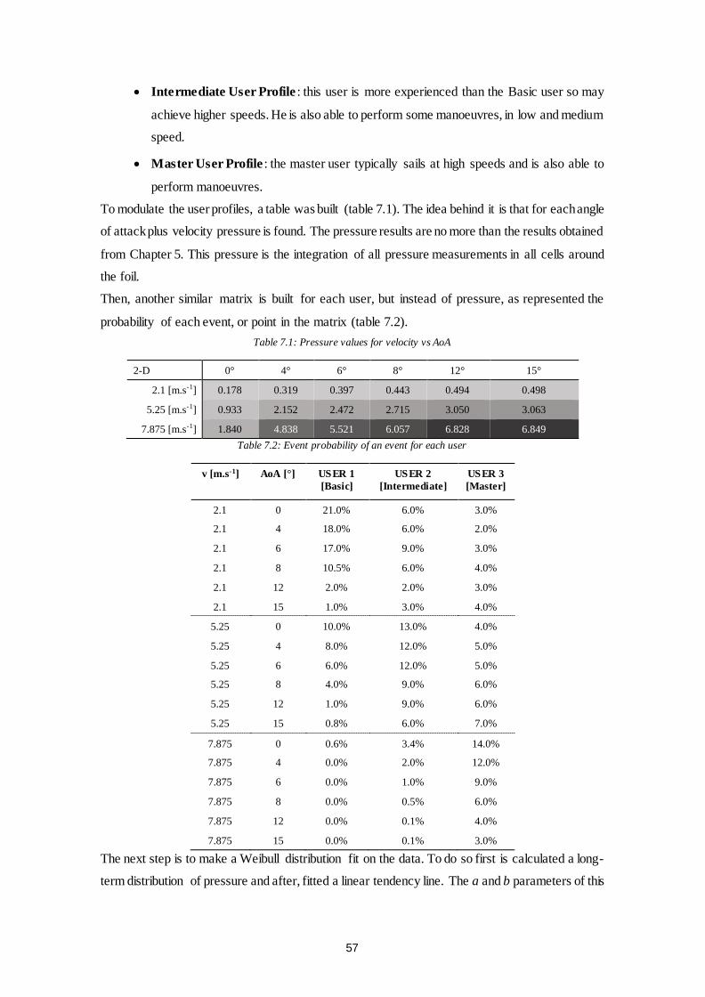
57
• Intermediate User Profile : this user is more experienced than the Basic user so may
achieve higher speeds. He is also able to perform some manoeuvres, in low and medium
speed.
• Master User Profile : the master user typically sails at high speeds and is also able to
perform manoeuvres.
To modulate the user profiles, a table was built (table 7.1). The idea behind it is that for each angle
of attack plus velocity pressure is found. The pressure results are no more than the results obtained
from Chapter 5. This pressure is the integration of all pressure measurements in all cells around
the foil.
Then, another similar matrix is built for each user, but instead of pressure, as represented the
probability of each event, or point in the matrix (table 7.2).
Table 7.1: Pressure values for velocity vs AoA
2-D 0° 4° 6° 8° 12° 15°
2.1 [m.s-1] 0.178 0.319 0.397 0.443 0.494 0.498
5.25 [m.s-1] 0.933 2.152 2.472 2.715 3.050 3.063
7.875 [m.s-1] 1.840 4.838 5.521 6.057 6.828 6.849
Table 7.2: Event probability of an event for each user
v [m.s-1] AoA [°] USER 1
[Basic]
USER 2
[Intermediate]
USER 3
[Master]
2.1 0 21.0% 6.0% 3.0%
2.1 4 18.0% 6.0% 2.0%
2.1 6 17.0% 9.0% 3.0%
2.1 8 10.5% 6.0% 4.0%
2.1 12 2.0% 2.0% 3.0%
2.1 15 1.0% 3.0% 4.0%
5.25 0 10.0% 13.0% 4.0%
5.25 4 8.0% 12.0% 5.0%
5.25 6 6.0% 12.0% 5.0%
5.25 8 4.0% 9.0% 6.0%
5.25 12 1.0% 9.0% 6.0%
5.25 15 0.8% 6.0% 7.0%
7.875 0 0.6% 3.4% 14.0%
7.875 4 0.0% 2.0% 12.0%
7.875 6 0.0% 1.0% 9.0%
7.875 8 0.0% 0.5% 6.0%
7.875 12 0.0% 0.1% 4.0%
7.875 15 0.0% 0.1% 3.0%
The next step is to make a Weibull distribution fit on the data. To do so first is calculated a long-
term distribution of pressure and after, fitted a linear tendency line. The a and b parameters of this

58
line are then converted in h and q for the distribution. Finally, the Weibull Distribution or the
cumulative frequency of each pressure for each sailing case is plotted (Figure 7.5).
(a) Basic User
(b) Intermediate User
(c) Master User
Figure 7.5: Weibull Distribution for the three user profiles
As expected, the basic user shows a higher probability of generating smaller pressures on the fin.
For the remaining users, the slope shifts to more considerable pressures, indicative of how each
profile manages its velocity/angle and associated pressure interval. These graphs are indicative
and shall be used on a later analysis, which will combine fatigue results.
7.3 Notes on Water Tunnel Results
Parallel to the CFD investigation, at the Emerson Cavitation Tunnel, in Newcastle University,
water tunnel tests have been conducted by Katherine Tansley [29].
On her research was used the same fin like the one used on this work. The flow speed and angle
of attack are changed to perform several hydrodynamic conditions. The analysis focused on the
flow around the fin and the flow transition on the surface. The loads are obtained with a six-
component load cell. The integral description of the assembly may be found at the disclosed work.
The main conclusions state that the fin enters in stall at 8° of AoA and lift is the main force
contributing to the resultant of forces. Additionally, it is verified that the fin tip deflects and that
this deflection rises with the flow velocity and AoA. This is an important conclusion, as the fin
geometry changes, so do the behaviour of the flow. It means that the results taken by CFD analysis
will lack this phenomenon, and those results will not portrait a realistic scenario. It will be vital
to perform a Fluid-Structure Interaction analysis to be closer to the real-life model.
It is also interesting to verify that the deflection does not seem to decrease after the fin stalls, as
one would expect after a reduction in lift.
The lift measurements are also hard to predict after 7°/8° AoA and lift is seen to be decreasing
after 13.5°. The results of the lift coefficient/lift force will be posteriorly compared when more
data from the CFD analysis is concluded, although the reader must bear in mind the differences
in experimental and analytical results.
0,00
0,20
0,40
0,60
0,80
1,00
0 2 4 6 8
Fl(
P2
-D)
P2-D [MPa]
0,00
0,20
0,40
0,60
0,80
1,00
0 2 4 6 8Fl(
P2
-D)
P2-D [MPa]
0,00
0,20
0,40
0,60
0,80
1,00
0 2 4 6 8
2-D
P2D [MPa]

59
Chapter 8
Conclusion
The objective of this thesis was to perform a hydrodynamic analysis and find how much load was
at play on a slalom fin of windsurf board. Since the shape of the fin’s hydrofoil cannot be fit into
any standard, like NACA for instance, it was mandatory to have a method to validate and calibrate
the three-dynamic analysis, instead of tackling the problem directly. Thus, the task was divided
into smaller tasks.
The first task was intended to feel in which regime the flow fitted. This is important, as later on
explained, to select the most appropriate physical model. In this first task, the program XFOIL
was used. The reasons to use XFOIL are multiple: it was chosen for being an open use software,
and also because most of the remaining programs use the same code foundation. It is also simple
and easy to use. Firstly, using a known aerofoil as control (an Eppler 387), the outputs from the
program were compared to real wind tunnel experiments. The choice of control aerofoil was set
not because of its geometry but because of the data available, which was inside the same Reynolds
number interval. Knowing the abilities and limitations of the program from the simulation, the
results from the fin hydrofoil were extracted. This was, most times, a hard task because the
convergence of results proved difficult for AoA’s between 4° and 5°. It was also needed to input
a modification on the geometry of the foil, to fix a Computer Aided Design problem. This small
difference in the profile geometry also shows how the manufacturing process is determinant.
Unfortunately, XFOIL cannot characterise laminar separation bubbles, and that was understood
as the reason for the difficulty felt to converge certain angles.
From those notes, the second part of the three-part objective was outlined. It was clear that a
transition model would have to be used, due to the flow regime and to the hint from the non-
convergence of results. A 2-D study was developed to understand which model would provide
the most accurate solution. To accomplish the job, the CFD program Star-CCM+ was used; a very
intuitive software available for researchers at the LASEF laboratory, in Lisbon. Again, the control
aerofoil was used for validation and determined that using RANS, the SST k – ω Turbulence
Model and the add-on γ – Reθ Transition Model would be a possible way to start the analysis. Of

60
course, there are many different models and solvers, each best suited for specific purposes. There
are many more combinations, although verifying each would take an extended period.
Attention was given to the mesh characterisation. The domain was divided into volumes, all
delimitating the space surrounding the foil. This way, the dimension of the mesh around the foil
could be fine-tuned, to meet the needs of the physics model and present quality results. The most
vital of these needs is to have a good boundary layer definition to capture the transition effects.
Thus, the mesh immediately around the foil needs to be constant and very fine. The method to
access this is by having a Wall Y+ parameter not more than 1.
In the end, lift and pressure distributions are accurate with the chosen physics’ models but should
be kept in consideration that drag is represented with an error of 5%. The results with the SFWB
hydrofoil revealed there was, in fact, a recirculation bubble that the XFOIL failed to represent.
There were some issues regarding 2-D solutions. From previous literature and knowledge, it was
expected that the foil would shed vortexes. After intensive research, the only vortexes generated
where at the first stages of the simulation, before the solution was converged. After several
seconds into the simulation, there were still no signs of vortex street. This conclusion was also
supported by the absence of significant pressure or force variations. It is believed that the flow
does have instability, especially for larger AoA’s, but one or both of the next possibilities might
be occurring: either the mesh is too coarse to capture instability phenomenon like a Kelvin
Helmholtz, or an unknown error was occurring during the simulation. Regardless, the results from
validation propose that the simulation was well carried out.
Using the Star CCM+ results from the 2-D analysis from the fin, a mesh convergence study was
done. It was possible to reduce the number of cells in about 75% and keep the results inside an
error margin of 5%. The most sensible parameter being the drag.
Having gathered another critical parameter, the 3-D simulation was assembled. It was designed
with all the notes and results from the previous chapters. Although the first goal was to use the
mesh parameters as closer to the previous simulations, it proved hard to include the third control
volume, that added a very fine mesh to the leading and trailing edge of the fin. This mesh was
made to compensate for the acute edges of the foil, that, due to its radius, deformed the important
cells at these areas. It was, eventually, obtained a simulation with around 10M cells.
Simulations at 3-D stage progress at a smaller pace than 2-D simulations, and, because of this and
other factors, only one simulation case is included on this thesis. The results from the first
condition are unveiling results close to the two-dimensional analysis, and displaying the same
flow characteristics, like the LSB.
In what concerns the parametric optimisation studies, no advantages are seen when changing the
maximum thickness or its position. The path was also opened for later study of user profiles, that
will need to be coordinated with a FEM analysis to the fin itself. The latter is presently being
developed.

61
Finally, the parallel research in Newcastle at the cavitation tunnel shows that the fin stalls at about
8° of AoA, a number met by this thesis simulations. It also shows that the most critical force in
the force resultant, measured in the SFWB, is the lift. The drag force only becomes more
expressive after reaching 14°, where it increases rapidly. The fin also deflects with the
hydrodynamic forces. Even after the fin stalls, the deflection does not seem to reduce, as would
be expected from the lack of lift force.

62

63
Chapter 9
Future Work
Concerning the next steps of the present work, there are some main points of focus that would be
interesting to explore.
This thesis may be extended in what concerns the 3-D simulation. More cases are under
development and when done, should provide an insight of the fin behaviour. The results will then
be compared to the real-life results obtained at the cavitation tunnel.
The remaining works being developed by peers are a good add-up for the understanding of the
fin. The finite element analysis that follows the hydrodynamic study in this work is already using
the data provided. In the future, it is also possible to pursue a fluid-structure interaction study, as
first intended, and vital to correctly model what occurs to the fin. This will provide results, not
only for hydrodynamic and structural behaviour but also, in real time, apply torsion. Due to this,
it will be possible to see the forces in the fin and how it flexes and bends back and changes the
fluid. With this dynamic, it will come clearer why and how the fin is breaking and make a more
accessible path to work on optimisation.
The hydrodynamic analysis also provided the tools and instructions for fin makers to reproduce
the water effects in a non-destructive test. With this, it will be possible to achieve an enhanced
fin, saving money in tests. This optimisation will give the real users improved speed and balance,
as well as an overall better-quality product for less price.
Regarding competition, it will prove to be the future tool for improving this vital part of the
windsurf board. Fins will be tailored for the players in less time, helping teams reach higher
scores.

64

65
References
[1] T. Talay, "Introduction to the Aerodynamics of Flight," NASA, 1975. [Online].
Available: https://history.nasa.gov/SP-367/cover367.htm. [Accessed 30 May
2018].
[2] L. Sutherland, "Windsurf Fins," 2018. [Online]. Available:
http://www.leighsutherland.com/index.html. [Accessed 2 May 2018].
[3] A. Center, "Technology, Invention and Innovation Collections," Archives Center,
National Museum of American History, August 1999. [Online]. Available:
https://web.archive.org/web/20150219204212/http://amhistory.si.edu/archives
/d8625.htm. [Accessed 19 February 2015].
[4] Arne, "When to use the centreboard," 2013. [Online]. [Accessed 26 March 2018].
[5] I. Sailboards, "Windsurfing 101: Understand fundamentals of windsurfing boards &
parts: Isthmus Sailboards," Isthmus Sailboards, 2018. [Online]. Available:
https://isthmussailboards.com/windsurfing-101. [Accessed 26 March 2018].
[6] E. /. S. Team, "Windsurfing Fins Basics," EASY / SURF shop, [Online]. Available:
https://easy-surfshop.com/do/page/buyingguide-fins. [Accessed 27 March 2018].
[7] F. Moukalled, L. Mangani and M. Darwish, The Finite Volume Method in
Computational Fluid Dynamics, vol. 113, Springer International, 2016.
[8] V. d. Brederode, Fundamentos de Aerodinâmica Incompressível, Lisboa: Author's
edition, 1997.
[9] N. M. Silva, Parametric Design, Aerodynamic Analysis and Parametric Optimization
of a Solar UAV, Lisbon: Instituto Superior Técnico, 2014.
[10] K. R. Atkins, Investigation into the flow behaviour of a NACA 0021 airfoil with leading
edge undulations simulated with RANS in Star-CCM+, Manchester: School of
Mechanical, Aerospace and Civil Engineering, 2015.

66
[11] F. Nascimento, Windsurf Fin- Numerical and Experimental Analysis of Ultimate
Strength, Lisbon: Instituto Superior Técnico, 2017.
[12] M. H. Sharqawy, J. H. Lienhard and S. M. Zubair, "Thermophysical properties of
seawater: A review and new correlations that include pressure dependance,"
Desalination and Water Treatment, vol. 16, pp. 354-380, April 2010.
[13] K. G. Nayar, M. H. Sharqawy, L. D. Banchik and J. H. Lienhard, "Thermophysical
properties of seawater: A review and new correlations that include pressure
dependance," Desalination, vol. 390, pp. 1-24, 2016.
[14] G. Cribb, "Tactics, Tuning and Technique," Windsurf, no. 298, 2010.
[15] N. Hall, "Navier-Stokes Equations," NASA, 5 May 2015. [Online]. Available:
https://www.grc.nasa.gov/www/k-12/airplane/nseqs.html. [Accessed 2 April
2018].
[16] H. Strum, G. Dumstorff, P. Busche, Dieter Westermann and W. Lang, "Boundary
Layer Separation and Reattachment Detection on Airfoils by Thermal Flow
Sensors," Sensors, vol. 11, 2012.
[17] H. Y. Mark Drela, Xfoil 6.94 User Guide, 2001.
[18] M. Hepperle, "Martin Hepperle," Dr. Martin Hepperle, 27 January 2007. [Online].
Available: https://www.mh-aerotools.de/airfoils/javafoil.htm. [Accessed 1 March
2017].
[19] Varius, "XFLR5," 7 January 2018. [Online]. Available:
http://www.xflr5.com/xflr5.htm. [Accessed 1 March 2018].
[20] S. B. W. a. F. B. M. J. R. MCGhee, Experimental Results for the Eppler 387 Airfoil at
Low Reynolds Numbers in the Lagley Low-Turbulence Pressure Tunnel, NASA TM-
4062, 1988.
[21] I. ANSYS, "ANSYS Fluent Sonftware: CFD Simulation," ANSYS, Inc, 2018. [Online].
Available: https://www.ansys.com/products/fluids/ansys-fluent. [Accessed 17
August 2018].

67
[22] Siemens, "STAR-CCM+ |MDX," Siemens, 2018. [Online]. Available:
https://mdx.plm.automation.siemens.com/star-ccm-plus. [Accessed 17 August
2018].
[23] O. L. (. Group), "OpenFOAM(R) - Official home of The Open Source Computational
Fluid Dynamics (CFD) Toolbox," OpenCFD Ltd, 2018. [Online]. Available:
https://www.openfoam.com/. [Accessed 16 August 2018].
[24] S. M. A. Aftab, A. S. Mohd Rafie, N. A. Razak and K. A. Ahmad, "Turbulence Model
Selection for Low Reynolds Number Flows," PLos ONE, vol. V. 11 (4), 2016.
[25] F. R. Menter, "Two-equation eddy-viscosity turbulence models for engineering
applications," vol. 32, no. 8, pp. 1598-1605, 1994.
[26] R. B. a. M. F. R. Langtry, "Correlation-based transition modeling for unstructured
parallelized computational fluid dynamics codes," AIAA, vol. 47, no. 12, pp. 2894-
2906.
[27] F. R. Menter, R. Langtry, S. Likki, Y. Suzen, P. Huang and S. Volker, "A correlation-
based transition model using local variables—Part I: model formulation," Journal
of turbomachinery, vol. 128, no. 3, pp. 413-422, 2006.
[28] P. Lissaman, "Low-Reynolds-number airfoils," Annual Review of Fluids Mechanics,
vol. Vol. 15, no. no. 1, pp. pp. 223-239, 1983.
[29] K. Tansley, "Investigation into Windsurf Fin Hydrodynamics - A practical Study,"
Newcastle University, Newcastle, 2018.

68

69
Appendix A
A.1 P113 Coordinates
x y x y x y x y x y
1 0.00065
0.58803 0.03723
0.16348 0.03195
0.17665 -0.03309
0.60132 -0.03664
0.99453 0.00138
0.57475 0.03778
0.15032 0.03071
0.18985 -0.03414
0.6146 -0.03601
0.98425 0.00275
0.56146 0.03829
0.13717 0.02937
0.20305 -0.0351
0.62788 -0.03535
0.9716 0.00446
0.54818 0.03877
0.12405 0.02791
0.21627 -0.03597
0.64116 -0.03464
0.95867 0.0062
0.53489 0.0392
0.11096 0.02633
0.2295 -0.03677
0.65443 -0.03389
0.94561 0.00793
0.5216 0.03959
0.09788 0.02462
0.24273 -0.03749
0.6677 -0.03311
0.93251 0.0096
0.50831 0.03993
0.08489 0.02277
0.25597 -0.03813
0.68098 -0.03229
0.91934 0.01119
0.49502 0.04024
0.07195 0.02075
0.26922 -0.03871
0.69425 -0.03142
0.90618 0.0127
0.48173 0.04051
0.0589 0.0185
0.28248 -0.03922
0.70751 -0.03053
0.89299 0.01413
0.46844 0.04074
0.04627 0.01608
0.29574 -0.03967
0.72078 -0.02959
0.87977 0.01552
0.45514 0.04092
0.03422 0.01349
0.309 -0.04005
0.73404 -0.02861
0.86653 0.01688
0.44185 0.04107
0.02222 0.0105
0.32227 -0.04038
0.7473 -0.0276
0.85329 0.0182
0.42856 0.04117
0.011 0.00713
0.33555 -0.04065
0.76056 -0.02656
0.84004 0.0195
0.41527 0.04123
0.00428 0.00444
0.34883 -0.04086
0.77382 -0.02547
0.8268 0.02077
0.40198 0.04125
0.00116 0.0023
0.36211 -0.04103
0.78707 -0.02436
0.81355 0.022
0.38869 0.04122
0.00012 0.00069
0.3754 -0.04115
0.80031 -0.0232
0.80031 0.0232
0.3754 0.04115
0.00012 -0.00069
0.38869 -0.04122
0.81355 -0.022
0.78707 0.02436
0.36211 0.04103
0.00116 -0.0023
0.40198 -0.04125
0.8268 -0.02077
0.77382 0.02547
0.34883 0.04086
0.00428 -0.00444
0.41527 -0.04123
0.84004 -0.0195
0.76056 0.02656
0.33555 0.04065
0.011 -0.00713 0.42856 -0.04117 0.85329 -0.0182
0.7473 0.0276
0.32227 0.04038
0.02222 -0.0105
0.44185 -0.04107
0.86653 -0.01688
0.73404 0.02861
0.309 0.04005
0.03422 -0.01349
0.45514 -0.04092
0.87977 -0.01552
0.72078 0.02959
0.29574 0.03967
0.04626 -0.01608
0.46844 -0.04074
0.89299 -0.01413
0.70751 0.03053
0.28248 0.03922
0.0589 -0.0185 0.48173 -0.04051 0.90618 -0.0127
0.69424 0.03142
0.26922 0.03871
0.07195 -0.02075
0.49502 -0.04024
0.91934 -0.01119
0.68098 0.03229
0.25597 0.03813
0.08489 -0.02277
0.50831 -0.03993
0.93251 -0.0096
0.6677 0.03311
0.24273 0.03749
0.09788 -0.02462 0.5216 -0.03959 0.94561 -0.00793
0.65443 0.03389
0.2295 0.03677
0.11096 -0.02633
0.53489 -0.0392
0.95867 -0.0062
0.64115 0.03464
0.21627 0.03597
0.12405 -0.02791
0.54818 -0.03877
0.9716 -0.00446
0.62788 0.03535
0.20305 0.0351
0.13717 -0.02937
0.56146 -0.03829
0.98425 -0.00275
0.6146 0.03601
0.18985 0.03414
0.15032 -0.03071
0.57475 -0.03778
0.99453 -0.00138
0.60132 0.03664
0.17665 0.03309
0.16348 -0.03195
0.58803 -0.03723
1 -0.00065