an upper extremity biomechanical model: application to the
TRANSCRIPT

Grand Valley State UniversityScholarWorks@GVSU
Masters Theses Graduate Research and Creative Practice
4-2007
An Upper Extremity Biomechanical Model:Application to the Bicep CurlAdam MillerGrand Valley State University
Follow this and additional works at: http://scholarworks.gvsu.edu/theses
Part of the Engineering Commons
This Thesis is brought to you for free and open access by the Graduate Research and Creative Practice at ScholarWorks@GVSU. It has been acceptedfor inclusion in Masters Theses by an authorized administrator of ScholarWorks@GVSU. For more information, please [email protected].
Recommended CitationMiller, Adam, "An Upper Extremity Biomechanical Model: Application to the Bicep Curl" (2007). Masters Theses. 686.http://scholarworks.gvsu.edu/theses/686
An Upper Extremity Biomechanical Model: Application to the Bicep Curl
A thesis by
Adam Miller, M.S.E. Presented April 2007
In partial fulfillment of the requirements for the Master of Science in Engineering degree
Advisor: Dr. Jeff Ray, Director of Engineering
School of Engineering Grand Valley State University
• Adam Miller 2007
Reproduced with permission of the copyright owner. Further reproduction prohibited without permission.

Grand Valley State University Padnos College of Engineering and Computing
CERTIFICATE OF EXAMINATION
Advisor Examining Board
)r. Shirley Fleischmann
Dr. Princewill Anyalebechi
The Thesis By
Adam Miller
entitled
Development of an Upper Extremity Biomechanical Model: Application to the Bicep Curl
is accepted in partial fulfillment of the requirements for the degree of Master of Science in Engineering
I H / V I a v ^00 fDate: Dr. C. Standridge, Graduate Director
Reproduced with permission of the copyright owner. Further reproduction prohibited without permission.

Development of an Upper Extremity Biomechanical Model: Application tothe Bicep Curl
aPadnos College of Engineering and Computing
M.S.E Thesis Presentation by
Adam MillerABSTRACT:
An upper extremity biomechanical model was developed based on
recommendations provided by the International Society of Biomecbanics. The model
was used to investigate biomecbanical differences between two variations of the bicep
curl exercise: the standing and incline dumbbell curls. An 8-camera Vicon motion
capture system was used to collect data on five subjects that executed 10 repetitions of
each type of curl.
Four key biomecbanical indicator variables were investigated: range of motion,
maximum elbow flexion moment, mean elbow flexion moment, and the flexion angle at
which the maximum flexion moment occurs. On average, the range of motion at the
elbow was 11.9° less for the incline curl. Both the mean and maximum elbow flexion
moments were significantly higher for the incline curl. Finally, the flexion angle at
which the maximum flexion moment occurred was 71.9° for the standing bicep curl and
35.1° for the incline bicep curl, a difference of 36.8°.
GRANDVkLII'YStai i . U m v i R s n V
11
Reproduced with permission of the copyright owner. Further reproduction prohibited without permission.

DEDICATION
For my family, my friends, and all those who have supported me through my
journey thus far. To my loving fiancée, Nikki, for keeping me sane, believing in me, and
putting up with the long hours I’ve spent working on my computer monitor tan.
I l l
Reproduced with permission of the copyright owner. Further reproduction prohibited without permission.

ACKNOWLEDGEMENTS
The author would like to express his sincere gratitude to his co-workers and peers
at Mary Free Bed Rehabilitation Hospital’s Motion Analysis Center: Dr. Krisanne
Chapin, Mitch Barr, and Dr. Gordon Alderink.
I would especially like to thank Dr. Krisanne Chapin for her advice and support
throughout the entirety of my graduate education. Without her I would not have reached
this point.
IV
Reproduced with permission of the copyright owner. Further reproduction prohibited without permission.

Table of Contents
List of Tables.......................................................................................................................... vii
List of Figures........................................................................................................................viii
List of Symbols and Abbreviations..........................................................................................x
1 Introduction........................................................................................................................1
1.1 Upper Extremity Anatomy........................................................................................ 1
1.2 Description of Joint Angles...................................................................................... 5
1.3 Estimation of Joint Centers of Rotation................................................................. 12
1.4 Application of Upper Extremity Models............................................................... 16
2 Methods........................................................................................................................... 21
2.1 Upper Extremity Model.......................................................................................... 21
2.1.1 Thorax Coordinate System............................................................................ 23
2.1.2 Scapula Coordinate System........................................................................... 24
2.1.3 Humerus Coordinate System......................................................................... 25
2.1.4 Forearm Coordinate System.......................................................................... 25
2.1.5 Hand Coordinate System............................................................................... 26
2.1.6 Dumbbell Coordinate System........................................................................ 27
2.1.7 Estimation of Shoulder Joint Center............................................................. 28
2.1.8 Joint Rotations................................................................................................ 29
2.2 Experimental Methods............................................................................................ 30
2.3 Statistical Methods...................................................................................................35
3 Results..............................................................................................................................37
V
Reproduced with permission of the copyright owner. Further reproduction prohibited without permission.
3.1 Bicep Curl Kinematics and Kinetics.....................................................................37
3.2 Statistical Test Results...........................................................................................40
4 Discussion......................................................................................................................44
4.1 Limitations..............................................................................................................45
4.2 Recommendations.................................................................................................. 52
5 Conclusion......................................................................................................................54
6 References......................................................................................................................55
Appendix A : Center of Rotation Calculation.......................................................................57
Appendix B ; Vicon BodyLanguage Code........................................................................... 60
Appendix C : MATLAB Code for Center of Rotation Caleulation.................................... 67
Appendix D : Bicep Curl Kinematies and Kinetics............................................................. 70
Appendix E : Biomechanical Indicator Box Plots................................................................75
VI
Reproduced with permission of the copyright owner. Further reproduction prohibited without permission.

List of Tables
Table 1 : Upper Extremity Model Marker Locations........................................................... 22
Table 2: Thorax Coordinate System......................................................................................24
Table 3: Scapula Coordinate System.....................................................................................24
Table 4: Humerus Coordinate System.................................................................................. 25
Table 5: Forearm Coordinate System................................................................................... 26
Table 6: Hand Coordinate System.........................................................................................27
Table 7: Dumbbell Coordinate System................................................................................. 28
Table 8: Shoulder Joint Angles..............................................................................................29
Tahle 9: Elbow Joint Angles.................................................................................................. 30
Table 10: Wrist Joint Angles................................................................................................. 30
Table 11 : Descriptive Statistics for Range of M otion......................................................... 40
Table 12: Descriptive Statistics for Maximum Flexion Moment....................................... 41
Table 13: Descriptive Statistics for Flexion Angle at Maximum Moment........................ 41
Table 14: Descriptive Statistics for Mean Flexion Moment................................................42
Table 15: Independent Samples t-test for Equality of Means..............................................43
Vll
Reproduced with permission of the copyright owner. Further reproduction prohibited without permission.

List of Figures
Figure 1: Shoulder Girdle Anatomy^^^.................................................................................... 3
Figure 2: Elbow Joint Anatomy^^^............................................................................................4
Figure 3; Hand and Wrist^^ ...................................................................................................... 5
Figure 4: Body Planes^^ ............................................................................................................6
Figure 5: Euler Angles " ...........................................................................................................7
Figure 6: Globographic Shoulder Representation^^^.............................................................. 9
Figure 7: Definition of Globograpbie Joint Angles^^^............................................................ 9
Figure 8: Elbow Joint Articulation^'^.....................................................................................11
Figure 9: Wrist Artieulation^^^................................................................................................ 12
Figure 10: Spherical Joint Center.......................................................................................... 14
Figure 11: Scapulotboracic M otion^....................................................................................19
Figure 12: Elbow Flexor MuseW^^.......................................................................................20
Figure 13: Upper Extremity Bony Landmarks Proposed by the ISB^^ ..............................21
Figure 14: Thorax Coordinate System^^ ............................................................................... 23
Figure 15: Scapula Coordinate System^* .............................................................................. 24
Figure 16: Humerus Coordinate System^* ............................................................................ 25
Figure 17: Forearm Coordinate System^^ ............................................................................. 26
Figure 18: Hand Coordinate System......................................................................................27
Figure 19: Dumbbell Coordinate System............................................................................. 28
Figure 20: Subject Marker Placement....................................................................................32
Figure 21: 8-Camera Vicon Motion Capture System..........................................................33
Vlll
Reproduced with permission of the copyright owner. Further reproduction prohibited without permission.

Figure 22: Incline Curl Bench (Preacher Bench)..................................................................35
Figure 23: Incline and Standing Bicep Curl Average Kinematics and Kinetics................ 39
Figure 24: Varying Moment Arm of Biceps^'^......................................................................45
Figure 25: Link Segment Model^^^.........................................................................................46
Figure 26: Subject #1 Bicep Curl Average Kinematics and Kinetics.............................. 70
Figure 27: Subject #2 Bicep Curl Average Kinematics and Kinetics.............................. 71
Figure 28: Subject #3 Bicep Curl Average Kinematics and Kinetics.............................. 72
Figure 29: Subject #4 Bicep Curl Average Kinematics and Kinetics.............................. 73
Figure 30: Subject #5 Bicep Curl Average Kinematics and Kinetics.............................. 74
Figure 31: Elbow Flexion Range of Motion Box Plot......................................................... 75
Figure 32: Maximum Flexion Moment Box P lo t.................................................................76
Figure 33: Flexion Angle for Maximum Moment Box Plot................................................76
Figure 34: Mean Flexion Moment Box Plot.........................................................................77
IX
Reproduced with permission of the copyright owner. Further reproduction prohibited without permission.

List of Symbols and Abbreviations
ISB...................................................................... International Society of Biomeehanies
EMG....................................................................Electromyography
CoR..................................................................... Center of rotation
R ..........................................................................Rotation matrix between two segments
Rx(0)....................................................................Rotation about axis “x” by an angle 0
n ...........................................................................Total number of time frames
m ..........................................................................Total number of markers
Pij......................................................................... Position of marker] at time frame i
ij...........................................................................Radius of sphere on which marker] moves
Cgeom.....................................................................Geometric error
Caig........................................................................Algebraic error
Reproduced with permission of the copyright owner. Further reproduction prohibited without permission.

1 Introduction
Application of upper extremity biomechanical modeling in both clinical and non-
clinical settings has been hindered by the complex range of movements at the shoulder
girdle and by the limitations of available technologies. This is not to say that there have
not been any useful motion analyses of the upper extremity, but the underlying problems
that have prevented widespread use still exist. Consequently, there is no general standard
to guide the development of upper extremity models. However, as motion analyses prove
to be ever more valuable in fields such as gait analysis, sport biomechanics, and
ergonomics, innovative modeling techniques and standards are being developed to
overcome the hurdles of upper extremity biomechanical modeling.
1.1 Upper Extremity Anatomy
The upper extremity consists of the trunk, head, neck, shoulders, arms, and hands.
The complex anatomy and range of motion of the upper extremity is largely responsible
for prohibiting the development of robust models. For this reason it is important to be
familiar with upper extremity anatomy, particularly the shoulder girdle, to gain insight
into the problem at hand.
The shoulder has the greatest range of motion of any joint in the body. Many people
mistakenly consider shoulder joint as one joint, when in actuality shoulder motion eomes
fi-om four distinct articulations. Figure 1 shows the anatomy of the shoulder girdle,
including its four major joints. These include the sternoclavicular, acromioclavicular,
and glenohumeral joints. The sternoclavicular joint is a saddle type joint that links the
1
Reproduced with permission of the copyright owner. Further reproduction prohibited without permission.
upper extremity to the torso. Artieulation oeeurs between the medial end of both
clavicles, the cartilage of the first ribs, and the sternum. The acromioclavicular joint
functions as a pivot point between the lateral end of the clavicle and the scapula, allowing
for movement of the arm above the head. This joint is held together by various ligaments
that run between both the coracoid and acromion processes of the scapula and the
clavicle. The extremely mobile glenohumeral joint, commonly called the shoulder, is a
ball and socket joint and links the humerus to the glenoid fossa of the scapula. Finally,
although the scapula and thorax do not have the structure of a typical joint, articulation
between these segments, or scapulothoracic motion, also contributes to shoulder motion.
These four separate articulations all contribute simultaneously to shoulder motion.
Understanding and describing the impact of any of these particular joint’s articulation on
the overall range of motion of the shoulder is one of the many challenges of upper
extremity modeling. In fact, many upper extremity models simply do not account for
these individual articulations. The shoulder is certainly the most challenging aspect of
upper extremity modeling.
Reproduced with permission of the copyright owner. Further reproduction prohibited without permission.

Acromioclavicularjoint Sternoclavicular
joint
Acromion of scapula Clavicle
Sternum
Scapula
Glenotiumeral joint
Scapulottioracicarticulation
Humerus
Figure 1 : Shoulder Girdle Anatomy[1]
The elbow joint is far simpler than the shoulder in terms of range of motion, but
anatomically speaking it is equally as complex. As shown in Figure 2, the two bones of
the forearm articulate with the distal end of the humerus at the elbow. Actually, the
elbow is composed of two separate joints: the humeroulnar and the humeroradial joints.
The humeroulnar joint is a true hinge joint. Articulation occurs between the proximal
end of radius and the distal end of the humerus. The radioulnar joint can be classified as
a ball-and-socket joint, although ligaments surrounding the elbow joint connect the radius
and ulna, preventing abduction or adduction of the radioulnar joint. However, the
structure of the elbow still allows for rotation of the forearm, or pronation and supination.
Reproduced with permission of the copyright owner. Further reproduction prohibited without permission.

Humerus
Lateralepicondyle
Capitulum
Head
Tuberosity —f— ?
Radius
Radialnotch
\
Trochlea
/Medial
epicondyle
Olecranon
Semilunar notch
Coronoid process
Tuberosity
Ulna
Radial styloid process
Ulnar styloid process
Figure 2: Elbow Joint Anatomy^^^
The hand and wrist compose one of the most complex set of joints in the human
body. Measuring the motion of each bone in the hand requires the development of a
specialized biomechanical model. In fact, most general upper extremity studies simply
treat the hand as one segment, ignoring movement in the fingers altogether. However, a
brief introduction of the anatomy of the hand is appropriate. As shown in Figure 3, the
wrist is the connection between the two bones of the forearm and the hand. The wrist is
essentially composed of two rows of short bones, called carpals, which allow for motion
Reproduced with permission of the copyright owner. Further reproduction prohibited without permission.

at the wrist. The metacarpal bones are the five long bones that connect the phalanges, or
fingers, to the wrist.
Distalphalanx
Middlephalanx
Proximalphalanx
Metacarpalbone
Distal phalanx
Proximalphalanx
Carpal------bones
R ad ius U lna
Figure 3: Hand and Wrist '^
1.2 Description of Joint Angles
Calculation of joint angles, or kinematics, is one of the essential fimctions of a
biomecbanical model. Joint angles are typically defined as the angular position of a body
segment with regard to the proximal segment. For example, knee joint angles would
refer to the angular position of the shank relative to the thigh. Measurement of joint
angles in three dimensions is very difficult, if not impossible, to achieve through
observation alone. This is one of the driving forces for using motion capture systems and
biomecbanical models to measure joint angles.
Perhaps the most challenging aspect of upper extremity modeling is the difficulty in
describing shoulder joint angles in clinically meaningful terms. Three dimensional
Reproduced with permission of the copyright owner. Further reproduction prohibited without permission.
rotations can be described using quaternions, Euler angles, or helical axes, however,
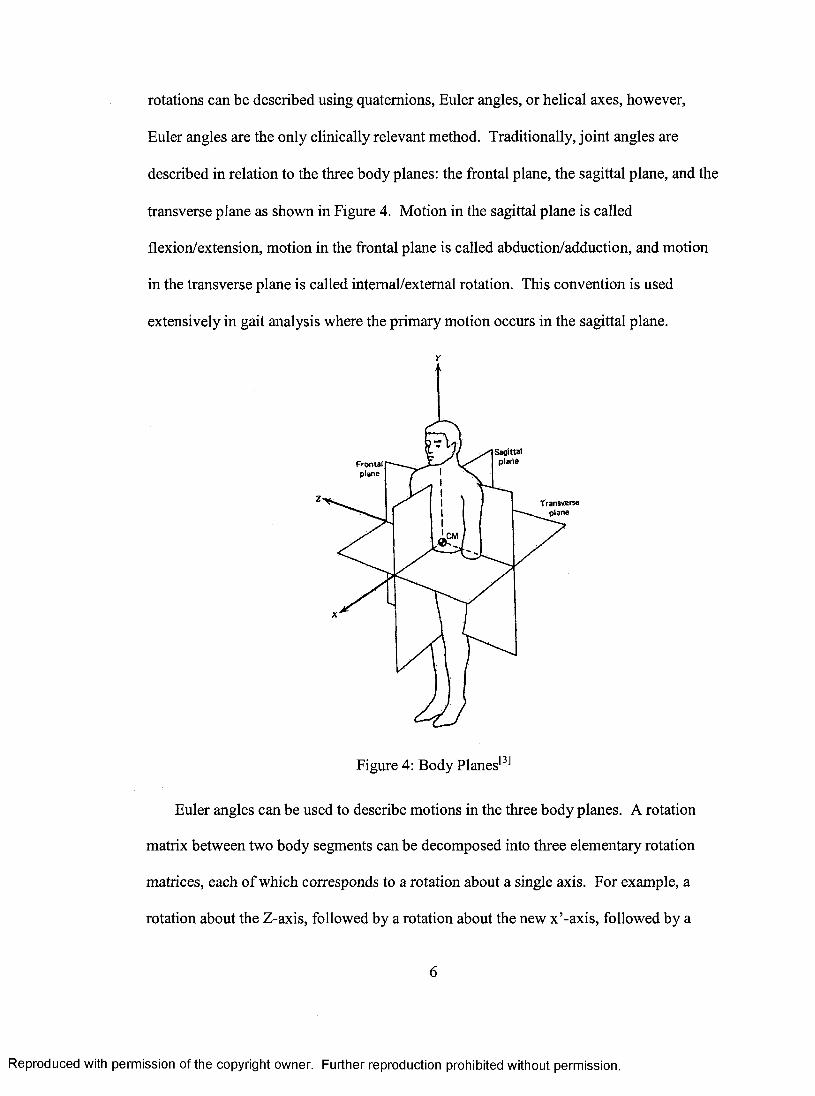
Euler angles are the only clinically relevant method. Traditionally, joint angles are
described in relation to the three body planes: the frontal plane, the sagittal plane, and the
transverse plane as shown in Figure 4. Motion in the sagittal plane is called
flexion/extension, motion in the frontal plane is called abduction/adduction, and motion
in the transverse plane is called intemal/extemal rotation. This convention is used
extensively in gait analysis where the primary motion occurs in the sagittal plane.
Sagittalplane
Z Transverseplane
Figure 4: Body Planes^^^
Euler angles can be used to describe motions in the three body planes. A rotation
matrix between two body segments can be decomposed into three elementary rotation
matrices, each of which corresponds to a rotation about a single axis. For example, a
rotation about the Z-axis, followed by a rotation about the new x ’-axis, followed by a
Reproduced with permission of the copyright owner. Further reproduction prohibited without permission.

rotation about the new z”-axis would be designated a (z”, x’, Z) Euler rotation sequence.
This is shown graphically in Figure 5 and mathematically in Equation 1.
R R,.M-RÀfyR,i'p)Where:
R = 3-dimensional rotation matrix
ip) = rotation about Z-axis by angle (p
Rx\o) - rotation about X’-axis by angle 0
= rotation about Z” -axis by angle y/
(1)
e abou t x '<p about 2
<|( about z"
Line of nodes
Figure 5: Euler Angles [4]
Reproduced with permission of the copyright owner. Further reproduction prohibited without permission.
In all there are twelve possible Euler rotation sequences that can be used to describe
the exact same rotation between two segments. The rotation sequence that should be
used is dictated by the type of motion being studied. For example, during gait, the hip,
knee, and ankle all articulate primarily about an axis perpendicular to the sagittal plane,
or the flexion/extension axis. For this reason the rotation order is chosen such that the
first rotation is about the flexion/extension axis, the second rotation is about the
ab/adduction axis, and the final rotation is about the long axis of a segment. This results
in rotation angles that closely mimic clinical measurements^^l
Upper extremity analysis differs in that there is no primary axis of rotation for the
shoulder. Instead, the primary axis of rotation depends on the motion being studied. For
example, during walking the primary rotation of the shoulder occurs about the
flexion/extension axis, but during throwing and lifting the primary rotation occurs about
the ab/adduction axis. When using Euler angles to describe shoulder joint angles, the
resulting angles for any given shoulder position will vary largely depending on the
rotation order used because of the interaction between the three variables necessary for
motion description^^l For this reason it is easy to understand why there is still no
universally accepted standard for the description of the shoulder joint angles. Some
models, such as the model developed by Williams et al. use a traditional
flexion/extension, ab/adduction approacb^^l The International Society of Biomecbanics
(ISB) recommends the use of an alternative metbod^^l As shown in Figure 6 and Figure
7, the ISB’s approach is a globographic approach in which the orientation of the upper
arm is described using three angles: plane of elevation, elevation, and rotation. However,
these angles are still calculated using Euler angles.
8
Reproduced with permission of the copyright owner. Further reproduction prohibited without permission.

Figure 6: Globographic Shoulder Representation'[9]
a . E levation Angle b. Rotation P lan e A ngle
Posterio r A spect
(Internat
External
G. Internai an ij External Rotation
Figure 7: Definition of Globographic Joint Angles'[9]
Reproduced with permission of the copyright owner. Further reproduction prohibited without permission.

The use of Euler angles to calculate joint angles presents an additional problem from
a numerical standpoint. There is a mathematical singularity, called gimbal lock, when the
second rotation angle is zero ' l In lower extremity analyses this is never an issue because
the range of motion is limited. This allows for the biomecbanical model to be designed
such a way that gimbal lock conditions will never occur. However, in upper extremity
analysis this is not the case because of the large range of motion of the shoulder. Gimbal
lock conditions are nearly unavoidable at the shoulder and must be dealt with on a case
by case basis. However, other joints in the upper extremity have relatively limited range
of motion and gimbal lock is not an issue.
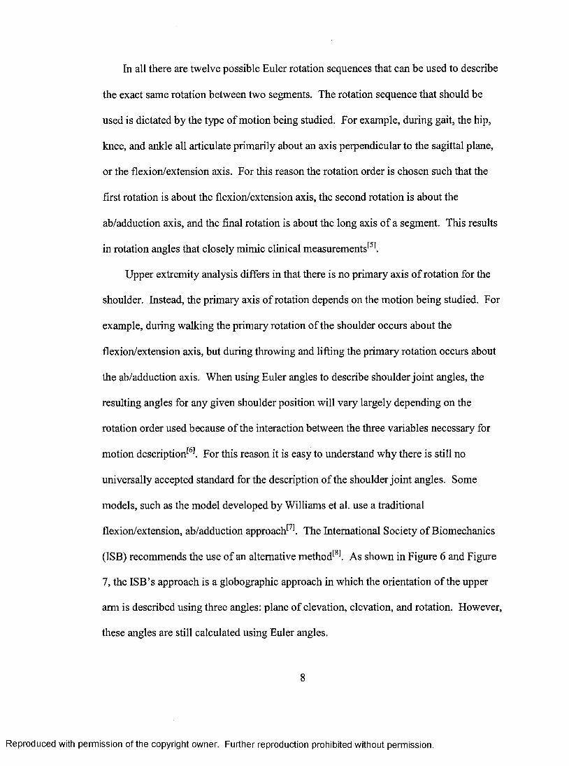
Description of elbow joint angles is relatively simple. The elbow is essentially a
hinge joint, although rotation about the long axis of the forearm also occurs. As shown in
Figure 8, elbow joint articulations are described as flexion/extension,
abduction/adduction, and pronation/supination. The primary axis of rotation for the
elbow is the flexion/extension axis, although significant axial rotation can also occur.
Abduction/adduction at the elbow is negligible and is rarely reported. In fact, this angle
remains constant and is defined as the carrying angle.
10
Reproduced with permission of the copyright owner. Further reproduction prohibited without permission.
Abduction/adduction
Humerus
X4
Flexion/extension
Radius
Ulna
Prdnatlon/supinationX4
Figure 8: Elbow Joint Articulation^'^
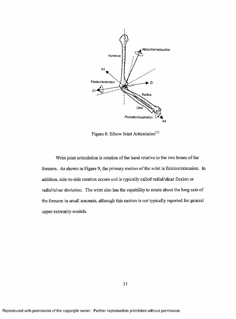
Wrist joint articulation is rotation of the hand relative to the two bones of the
forearm. As shown in Figure 9, the primary motion of the wrist is flexion/extension. In
addition, side-to-side rotation occurs and is typically called radial/ulnar flexion or
radial/ulnar deviation. The wrist also has the capability to rotate about the long axis of
the forearm in small amounts, although this motion is not typically reported for general
upper extremity models.
11
Reproduced with permission of the copyright owner. Further reproduction prohibited without permission.
Flexion
Extension
Hyperextension
Radial flexion
UInar flexion
Figure 9: Wrist Articulation^^^
1.3 Estimation of Joint Centers of Rotation
As with any link-segment biomechanical model, joint centers of rotation must be
determined for the various segments in the model. This is particularly difficult for the
glenohumeral joint because the joint center is hidden beneath soft tissue and the scapula.
However, several methods have been developed for estimating the position of the
shoulder joint center relative to surface markers. Some methods are only crude estimates
of the true rotation center. For example, one biomecbanical model uses a simple method
in which the joint center is located inferior to the acromion process’ A n o t h e r popular
method utilizes a regression equation that locates the glenohumeral joint center in relation
to palpable bony landmarks of the seapuW^^l However, the majority of models utilize
some type of functional method to locate the joint center. Functional methods require the
subject to move through a predetermined range of motion, during which time motion
capture data is collected. This data is then used to locate the joint center using
12
Reproduced with permission of the copyright owner. Further reproduction prohibited without permission.
mathematical techniques. All of these methods assume that the shoulder acts as a perfect
ball and socket joint, thus a single point can be used as the center o f rotation. For
example, Veeger et al. used the optimum pivot point of helical axes to locate the joint
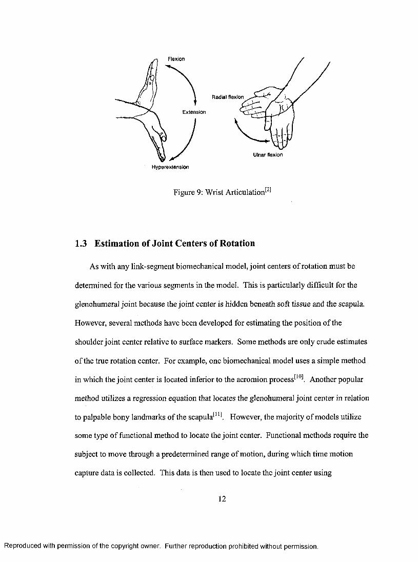
center^'^l Another method, a sphere fitting method, seeks to find the optimum rotation
point by fitting a sphere to the motion capture data. Several forms of the sphere fitting
method have been developed. One of the first methods developed uses least squares
optimization to minimize geometric error, Cgeom, to find the optimum center of rotation.
For example, for i = 1,..., n time frames and j = 1,..., m markers, the center of rotation,
CoR, is determined using marker positions, pÿ, and the radius, rj, of the sphere on which
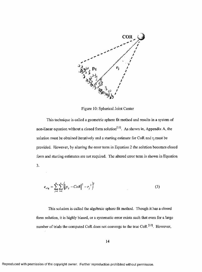
marker j moves. This is illustrated in Figure 10 and shown mathematically in Equation 2.
= É Ê Ik - - - 0 ] (2)J = \ (=1
13
Reproduced with permission of the copyright owner. Further reproduction prohibited without permission.
COR ,
Figure 10: Spherical Joint Center
This technique is called a geometric sphere fit method and results in a system of
non-linear equation without a closed form solution^^^l As shown in, Appendix A, the
solution must be obtained iteratively and a starting estimate for CoR and rj must be
provided. However, by altering the error term in Equation 2 the solution becomes closed
form and starting estimates are not required. The altered error term is shown in Equation
3.
7=1 1=1
(3)
This solution is called the algebraic sphere fit method. Though it has a closed
form solution, it is highly biased, or a systematic error exists such that even for a large
number of trials the computed CoR does not converge to the true CoR However,
14
Reproduced with permission of the copyright owner. Further reproduction prohibited without permission.

Halvorsen investigated this problem and created an iterative method for eliminating the
bias^ ' l His method is advantageous in that it does not require an initial estimate of CoR
and in terms of accuracy it is equivalent to the geometric sphere fit method.
Several studies have been performed to determine the repeatability and accuracy
of various methods for determining joint centers of rotation. Stokdijk et al. performed
repeatability studies on the regression method, the sphere fit method, and the helical axes
method^^^l The study showed that the regression method has poor intra-observer
reliability due to variability in marker placement. It was also noted that the regression
method is not applicable for patients with osseous deformation of the scapula or humeral
head. The spherical and helical axes methods were equivalent in terms of intra and inter
observer reliability. Ehrig et al. simulated data for the helical and geometric sphere fit
methods in various scenarios in which noise was introduced and range of motion was
limited^^^l The study showed that error for all methods increases approximately
exponentially as range of motion is decreased and that the helical axes method is more
accurate than the spherical method, especially when range of motion is limited to less
than 45°. The helical axes technique is favored by the majority of researchers, not only
because of its accuracy, but also because it is also capable of estimating the axis of
rotation for hinge joints, such as the elbow and knee.
The methods discussed previously, with exception of the regression method, can
be applied to any joint in the human body. However, simple estimation techniques are
often used in favor of mathematical techniques when possible. For example, the elbow
joint center can be estimated by finding the midpoint of the line between the medial and
lateral epicondyles of the humerus. This is a simple, effective method that can also be
15
Reproduced with permission of the copyright owner. Further reproduction prohibited without permission.

applied to the wrist, knee, and ankle where prominent bony landmarks are present on
both sides of the center of rotation. However, mathematical techniques, such as the
helical axes method, can be used to improve accuracy, but this comes at the expense of
increased processing and computing time.
1.4 Application o f Upper Extremity Models
To date, there have been significantly fewer applications of upper extremity
biomechanical models than there have been for the lower extremity models. However,
upper extremity models can be used much the same as lower extremity models. For
instance, one of the primary roles of lower extremity models is gait analysis, in which the
gait patterns of subjects with movement disorders are quantitatively analyzed. This
quantitative analysis takes the guesswork out of making clinical decisions and has been
used extensively for children with cerebral palsy^^^l For example, orthopedic problems
such as bony rotations, muscle spasticity, and muscle contracture can all contribute to
abnormal gait, making it difficult to determine the most effective treatment option. Gait
analysis is used to separate the different components of gait, allowing for the best
treatment to be pursued. Furthermore, gait analysis can be used to make quantitative
assessment of a patient’s walking pattern pre and post treatment to assess the efficacy of
a given treatment. Gait analysis can be applied to any ambulatory individual, including
those with prosthetic limbs. Upper extremity models can be used for similar purposes.
Several studies have been conducted that demonstrate the potential uses of upper
extremity biomechanical models. One study investigated the upper extremity function of
children with plexus lesions caused by birth t r a u m a ^ I n the study, children were fitted
with surface markers and EMG electrodes and asked to reach for a cookie with both their
16
Reproduced with permission of the copyright owner. Further reproduction prohibited without permission.

normal and pathologie arms. The biomechanical model alone indicated how the
movement pattern was altered due to the impairment. When combined with surface
EMG, the effects of missing muscular contraction, co-contraction, or mechanical
blockage of the joints were apparent. This information is crucial for the planning of
conservative and surgical therapies. Another model was developed and used to compare
upper extremity movement in children with cerebral palsy to that of normal childrens'll
Data on a group of normal subjects was collected, averaged, and compared to the
movement of children with cerebral palsy. This allowed for conclusions to be made about
the causes of abnormal movement patterns. However, upper extremity analysis is not
limited to the study of pathologic movement. They can also be used in sports
applications. Upper extremity models have successfully been used in several sports such
as golf, baseball, teimis, and cricket for purposes ranging from injury prevention to
identification of effective training methods^'^’ ^l Finally, although relatively unexplored,
upper extremity models can also be used to access workplace ergonomics, generating
safe working environments for office and factory workers alike^^^l It is clear that there
are many potential uses for upper extremity biomechanical models, however,
development and application of biomechanical models is not a simple step.
Human gait is a highly cyclic, pattem-like motion. This allows for time
normalization or kinematics and kinetics and calculation of temporal spatial parameters
such as walking velocity, stride length, and cadence. Upper extremity function varies
widely when compared to lower extremity function. Typical motions include the use of
tools, performing complex manipulations, throwing objects, pointing, making gestures,
feeding, and grooming. Theoretically, motion analysis could be done on any of these
17
Reproduced with permission of the copyright owner. Further reproduction prohibited without permission.

motions or any other upper extremity motion, indicating that it is necessary to establish a
standard set o f experimental movements from which clinical conclusions can be drawn.
However, not only do the types of motions differ, but there is also high variability in the
way that each individual accomplishes a specific task. In addition, these problems are
exacerbated by the fact that the wide range of movements in the upper extremity
increases the potential for skin and soft tissue artifact in motion capture data.
Skin and soft tissue movements are a major limitation to surface marker based
motion analysis. Movement of surface markers relative to the bony landmarks they are
intended to track generates skin movement artifacts in motion capture data. In gait
analysis this is typically not a problem because the lower extremity is relatively lean and
there is an abundance of prominent bony landmarks. However, in the upper extremity,
skin movement artifacts can cause problems, especially with regard to axial rotations and
scapulothoracic motion. In fact, axial rotation can be underestimated by as much as 35%
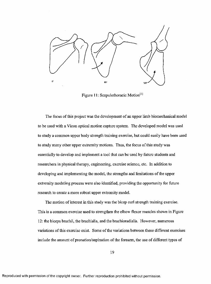
due to soft tissue movement^^^l Also, as shown in Figure 11, the motion of the scapula
becomes significant when the arm is elevated above horizontal, meaning that the
accuracy of skin based markers placed over the scapula is severely compromised when
observing overhead motions. Problems aside, it is still possible to develop and
implement robust upper extremity models.
18
Reproduced with permission of the copyright owner. Further reproduction prohibited without permission.
/
0 °
Figure 11: Scapulothoracic Motion' '^
The focus of this project was the development of an upper limb biomechanical model
to be used with a Vicon optical motion capture system. The developed model was used
to study a common upper body strength training exercise, but could easily have been used
to study many other upper extremity motions. Thus, the focus of this study was
essentially to develop and implement a tool that can be used by future students and
researchers in physical therapy, engineering, exercise science, etc. In addition to
developing and implementing the model, the strengths and limitations of the upper
extremity modeling process were also identified, providing the opportunity for future
research to create a more robust upper extremity model.
The motion of interest in this study was the bicep curl strength training exercise.
This is a common exercise used to strengthen the elbow flexor muscles shown in Figure
12: the biceps brachii, the brachialis, and the brachioradialis. However, numerous
variations of this exercise exist. Some of the variations between these different exercises
include the amount of pronation/supination of the forearm, the use of different types of
19
Reproduced with permission of the copyright owner. Further reproduction prohibited without permission.

barbells or dumbbells, the use of methods to stabilize the upper arm, and the orientation
of hoth the thorax and the upper arm during the exercise. Oddly enough, there are more
variations of the exercise than there are elhow flexor muscles. This raises the question as
to why there are so many different exercises when the function of the muscles does not
change. For this reason, two of the most common variations of the hicep curl, the
standing dumbbell and the preacher dumbbell curl, were chosen as candidates for a
biomechanical study. In this study key biomechanical indicators, such as range of
motion, maximum flexion moment, and mean flexion moment were measured, from
which conclusions can he drawn ahout implications on the exercise physiology of hoth
variations.
Biceps (short ■ head)
(long _ head)
Fibrous locertus
Deitoid
111
Brochtolis
Brochioradiolis
Supinator
Pronator
Figure 12: Elhow Flexor Muscles^^^
20
Reproduced with permission of the copyright owner. Further reproduction prohibited without permission.

2 Methods
2.1 Upper Extremity Model
The model developed in this project was based on the standards proposed by the
ISB for upper extremity modeling^* . As shown in Figure 13, the ISB provides a set of
bony landmarks that should be used to define body segment coordinate systems as well as
recommendations on how joint rotations should be defined. The bony landmarks
described by the ISB along with other marker locations used for this study are described
in detail in Table 1.
Incisura Ju§ulans (U) Proc®s«us Xiphoideus (PX)Art. Stemockvkulaure (SC)
Afl Acronfiioclavicufere (AC)
Tr^onwm Scapulae (TS) Amguhis Infmor (Al) gulus AcronWaKs (AA)
rocessus coracoideus (PC) lenohumerii mtatkm centre (
lateral epicomdyle (EL)
Medial eptcondyie (EM)
l%M#ds%A*M(RS)
mnarstvWdtUS)
Figure 13: Upper Extremity Bony Landmarks Proposed by the ISB *
21
Reproduced with permission of the copyright owner. Further reproduction prohibited without permission.

Table 1 : Upper Extremity Model Marker Locations
H e a d
L F H D ^ Left, fron t h e a d jLBHD Left, b a c k h e a d |R FH D ' Right, fro n t h e a d |RBH D Right, b a c k h e a d |
T h o r a x
PX P ro c e s s u s X ip h o id eu s (xiphoid p ro c e s s ) , | m o s t c a u d a l po in t on th e s te rn u m |
Ü In c isu ra ju g u ia ris , ju g u la r no tch |C 7 ^ 7th c erv ica l v e r tib ra e |T 8 8th th o ra c ic v e r tib ra e I
S c a o u la
AC M ost d o rsa l po in t on th e a cro m io c lav icu la r jo in t ( s h a re d w ith th e s c a p u la )
T S
f rigonum S p in a e S c a p u la e (roo t o f th e | sp in e ), th e m idpo in t o f th e tr ian g u la r s u r fa c e j on th e m ed ia l b o rd e r o f th e s c a p u la in line 1 with th e s c a p u la r s p in e {
Al A n g u iu s Inferior (inferior an g le ), m o s t c a u d a l j po in t o f th e s c a p u la |
AA A n g u iu s A crom ia lis (acrom ia l an g le ) , m o s t j la te ro d o rsa l po in t o f th e s c a p u la |
P C1
M ost v e n tra l po in t o f p ro c e s s u s c o ra c o id e u s j
GH G le n o h u m e ra l ro tation c e n te r , e s t im a te d by j re g re s s io n o r m otion re c o rd in g s j
EL M o st c a u d a l po in t o n la te ra l ep ico n d y leEM Most c a u d a l po in t o n m ed ial ep ico n d y le |
F o re a rm
R S M ost c a u d a l- la te ra T po in t on th e rad ia l j styloid j
U S M ost c a u d a l-m e d ia l po in t on th e u ln a r j styloid i
W 1A nterio r a s p e c t o f w rist, m idw ay b e tw e e n R S j a n d U S I
W 2P o s te r io r a s p e c t o f w rist, m idw ay b e tw e e n j R S a n d U S 1
H a n d FINM iddle o f third m e ta c a rp a l on p o s te r io r s id e j o f h a n d |
HCH an d c e n te r , e s t im a te d from FIN o r m idpoint] o f DBE1 a n d D B E 2 I
D u m b b e ll
DBE1 E nd o f dum bbell, c e n te re d on long a x is
D BE2O p p o s ite e n d o f dum bbell, c e n te re d on long j a x is
DBC1C irc u m fe re n c e o f dum bbell, p la c e d on i w e ig h t p la te
DBC2C irc u m fe re n c e o f dum bbell, p la c e d on j w eig h t p la te on o p p o s ite e n d
22
Reproduced with permission of the copyright owner. Further reproduction prohibited without permission.

The model developed in this study was intended for use with a Vicon motion
capture system and Vicon biomechanical modeling software. Thus, the model developed
was written in Body Language, a proprietary language developed by Vicon to simplify
rigid body mechanics. The code for the model can be seen in Appendix B. The model
differed slightly from the recommendations provided by the ISB in some ways. A head
segment was added to the model for visualization purposes alone, thus exact
standardization of marker placement was never defined. In addition, no clavicle segment
was defined in this model, so there was no need to include sternoclavicular joint markers.
Finally, the addition of the hand and dumbbell segments was done entirely for the
purposes of studying bicep curl motion. The following sections detail how each body
segment was defined relative to the bony landmarks listed in Table 1.
2.1.1 Thorax Coordinate System
The thorax coordinate system (X*, Yt, Zt) is shown in Figure 14 and is defined in
Table 2.
Yt
Lsrteirgil
Figure 14: Thorax Coordinate System^*^
23
Reproduced with permission of the copyright owner. Further reproduction prohibited without permission.
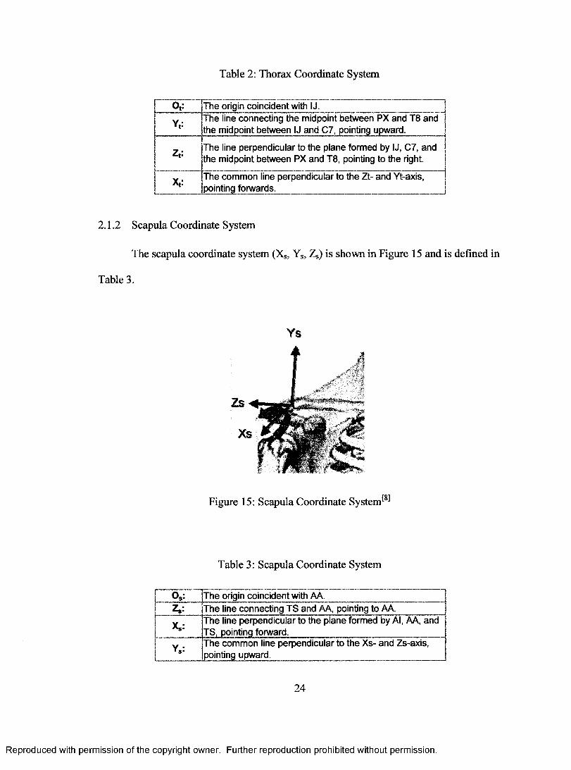
Table 2: Thorax Coordinate System
o ; : T h e origin c o in c id e n t with IJ.
Y,: T h e line c o n n ec tin g th e m idpo in t b e tw e e n PX a n d T 8 a n d th e m idpo in t b e tw e e n IJ a n d C 7, pointing upw ard .
Zt:T h e line p e rp e n d ic u la r to th e p la n e fo rm ed by IJ, C 7 , a n d th e m idpo in t b e tw e e n PX a n d T8, pointing to th e right.
Xt:T h e c o m m o n line p e rp e n d ic u la r to th e Zt- a n d Y t-axis, poin ting fo rw ards.
2.1.2 Scapula Coordinate System
The scapula coordinate system (X,, Ys, Zg) is shown in Figure 15 and is defined in
Table 3.
Ys
Figure 15; Scapula Coordinate System^*^
Table 3: Scapula Coordinate System
O s : T h e origin c o in c id e n t w ith AA.T h e line c o n n ec tin g T S a n d AA, pointing to AA.
X s :T h e line p e rp e n d ic u la r to th e p la n e fo rm ed by Al, AA, a n d T S , poin ting forw ard .
Y s :T h e c o m m o n line p e rp e n d ic u la r to th e X s- a n d Z s-ax is , poin ting upw ard .
24
Reproduced with permission of the copyright owner. Further reproduction prohibited without permission.

2.1.3 Humeras Coordinate System
The humeras coordinate system (Xh, Yj,, Zh) is shown in Figure 16 and is defined
in Table 4.
Plane of elevation Negative eletmtion Axial rotation
Figure 16: Humerus Coordinate System^*^
Table 4: Humerus Coordinate System
T h e origin c o in c id e n t w ith GH.
Yh:T h e line c o n n e c tin g G H a n d th e m idpo in t o f EL a n d EM, pointing to GH.
Xh: T h e line p e rp e n d ic u la r to th e p la n e fo rm ed by EL, EM, a n d GH , poin ting forw ard .
Zh:T h e c o m m o n line p e rp e n d ic u la r to th e Y h1- a n d Z h1 -ax is , po in ting to th e right.
2.1.4 Forearm Coordinate System
The forearm coordinate system (Xf, Yf, Zf) is shown in Figure 17 and is defined in
Table 5.
25
Reproduced with permission of the copyright owner. Further reproduction prohibited without permission.

Figure 17: Forearm Coordinate System^*^
Table 5: Forearm Coordinate System
T h e origin c o in c id e n t w ith th e m idpo in t o f U S a n d R S .
Yf:T h e line c o n n e c tin g th e m idpo in t o f U S a n d R S a n d th e m idpo in t b e tw e e n EL a n d EM, poin ting proxim aily.
Xf:
Zf:
T h e line p e rp e n d ic u la r to th e p la n e th ro u g h th e m idpoin t o f U S a n d R S , R S , a n d th e m idpo in t b e tw e e n EL a n d EM, pointing forw ard .T h e c o m m o n line p e rp e n d ic u la r to th e Xf a n d Yf -ax is , poin ting to th e right.
2.1.5 Hand Coordinate System
The hand coordinate system (Xh, Yh, Zh) is shown in Figure 18 and is defined in
Table 6. In this study the hand center, HC, was estimated using the midpoint of DBEl
and DBE2. A dummy hand segment was first defined using this midpoint as the hand
origin. An estimate of the actual hand center was then located a predetermined distance
in the ‘X’ direction of the dummy coordinate system. The new hand center was then
used to define the actual hand segment.
26
Reproduced with permission of the copyright owner. Further reproduction prohibited without permission.

Yh
Zh
Figure 18: Hand Coordinate System
Table 6: Hand Coordinate System
T h e origin c o in c id e n t w ith HCT h e line c o n n ec tin g th e m idpoin t o f U S a n d R S a n d HC,
o in ting proxim aily_______________________________T h e line p e rp e n d ic u la r to th e p la n e th ro u g h U S, R S , a n dHÇ____________________________________________T h e c o m m o n line p e rp e n d ic u la r to th e Xh a n d Y h -ax is , po in ting to th e right._______________________
2.1.6 Dumbbell Coordinate System
The dumbbell coordinate system (Xd, Ya, Za) is shown in Figure 19 and defined in
Table 7. In this study the orientation of the dumbbell coordinate system was irrelevant
provided that the X-axis was along the long axis of the dumbbell.
27
Reproduced with permission of the copyright owner. Further reproduction prohibited without permission.

Figure 19: Dumbbell Coordinate System
Table 7: Dumbbell Coordinate System
Od: T h e origin c o in c id e n t w ith th e m idpo in t o f DBE1 a n d DBE2
Xd:T h e line c o n n e c tin g DBE1 a n d D B E 2 in th e m ed io -la te ra l d irection .
Yd:T h e line p e rp e n d ic u la r to th e p la n e th ro u g h D BE1, DBE2, a n d DBC1
Zd:T h e c o m m o n line p e rp e n d ic u la r to th e Xd a n d Yd -ax is
2.1.7 Estimation of Shoulder Joint Center
In this study the geometric sphere fit method was used to estimate the center of
rotation of the glenohumeral joint in the scapular coordinate system. After each subject
was fitted with markers he or she was asked to move through a specified range of motion.
This range of motion included three cycles of fiexion/extension, three cycles of
ab/adduction, and 3 cycles of circumduction. The subject was instructed not to raise their
arm above horizontal during any of these motions to minimize scapulothoracic motion
28
Reproduced with permission of the copyright owner. Further reproduction prohibited without permission.

and skin movement artifacts. After data capture the position of both EL and EM was
calculated in the scapular coordinate system for each frame of collected data. The
method shown in Appendix A was then implemented in MATLAB to estimate the
shoulder joint center. The code used can be seen in Appendix C.
2.1.8 Joint Rotations
In this study the only joint angles of interest were shoulder joint angles, elbow
joint angles, and wrist joint angles. All joint angles were calculated relative to the
proximal segment.
Shoulder joint angles were measured as the position of the humerus relative to the
thorax, also known as humerothoracic motion, and were calculated using a Y-X-Y Euler
rotation order as defined in Table 8.
Table 8: Shoulder Joint Angles
S h o u ld e r (YXY O rd e r)R o ta t io n A x is R e le v a n c e
1 YtP la n e o f e leva tion , 0° is ab d u c tio n , 90° is fo rw ard flexion
2 Xt E levation (n eg a tiv e )
3 YhIn ternal (positive) a n d E x ternal (n eg a tiv e ) ro tation
Elbow joint angles were calculated using a ZXY Euler rotation order as described
in Table 9.
29
Reproduced with permission of the copyright owner. Further reproduction prohibited without permission.

Table 9: Elbow Joint Angles
Elbow (ZXY Order)Rotation Axis Reievance
1 Zh Flexion (positive)
2 Floating C arry ing a n g le , ra re ly re p o rte d
3 Yf P ro n a tio n (positive) a n d S u p in a tio n (n eg a tiv e )
Wrist joint angles were calculated using a ZXY Euler rotation order as described
in Table 10.
Table 10: Wrist Joint Angles
Wrist (ZXY Order)Rotation Axis Reievance
1 Zf Flexion (positive)
2 Floating U lnar (positive) a n d rad ia l (n e g a tiv e ) dev ia tion
3 Yh Invalid in th is m odel
2.2 Experimental Methods
Five subjects above 18 years of age were recruited for the study based on the
guidelines proposed to and agreed upon by the Grand Valley State University Research
Subjects Review Committee (Proposal 07-97-H). Informed consent, media release, and
background information forms were reviewed and signed by each subject before
participation in the study.
After the required forms were completed by a subject, he or she was asked to
change into attire that bared their entire right arm and minimally covered their chest and
30
Reproduced with permission of the copyright owner. Further reproduction prohibited without permission.

back. This allowed for accurate placement of retroreflective markers used by the motion
capture system in this study. Height, weight, right hand thickness, and right hand length,
were then measured, although height was never explicitly used in this study. A dumbbell
was then loaded with weight plates such that it weighed as close as possible to 10% of the
subject’s body weight. Finally, the subject and dumbbell were fitted with retroreflective
markers as described in Table 1 and shown in Figure 20.
31
Reproduced with permission of the copyright owner. Further reproduction prohibited without permission.

Figure 20: Subject Marker Placement
32
Reproduced with permission of the copyright owner. Further reproduction prohibited without permission.

An 8-camera Vicon MCam2 motion capture system, shown in Figure 21, was set
up and calibrated before each subject’s arrival. This system captures data at a rate of 60
frames per second. In addition, two digital video camcorders were used to
simultaneously record video of the frontal and sagittal planes during data collection.
Figure 21: 8-Camera Vicon Motion Capture System
Each subject was first asked to perform a static trial in which he or she stood in
the anatomic neutral position for approximately 30 seconds. This trial was used to verify
placement of all markers and to ensure that the motion capture system was operating
properly. Second, each subject was asked to sit on a bench in the center of the motion
capture volume while he or she moved their shoulder through a specified range of motion
33
Reproduced with permission of the copyright owner. Further reproduction prohibited without permission.
as described in section 2.1.7. This trial was used for the purpose of estimating the
shoulder joint center. Finally, the subject was asked to perform a total of 20 dumbbell
curl repetitions, 10 of which were standing curls and 10 of which were incline curls. The
order in which these curls were performed was randomized using a computer program.
For example, a subject may have had to perform 2 standing curls, then 1 incline curl, then
1 standing curl, and then 3 incline curls, etc., until all 20 repetitions had been completed.
Both the standing and incline curls were executed such that the forearm started and ended
in a supinated (palm upward) position. In addition, subjects were allowed to self select
the speed at which they performed the dumbbell curl.
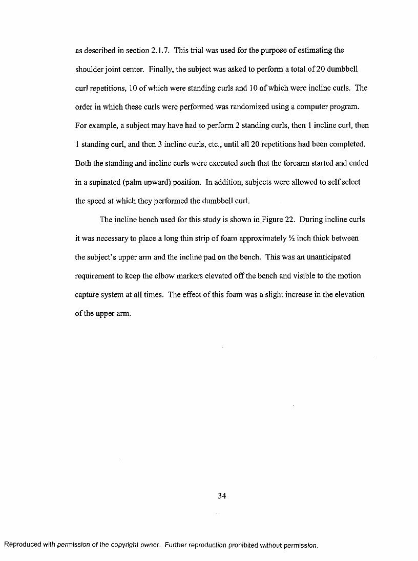
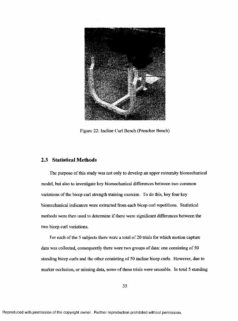
The incline bench used for this study is shown in Figure 22. During incline curls
it was necessary to place a long thin strip of foam approximately % inch thick between
the subject’s upper arm and the incline pad on the bench. This was an unanticipated
requirement to keep the elbow markers elevated off the bench and visible to the motion
capture system at all times. The effect of this foam was a slight increase in the elevation
of the upper arm.
34
Reproduced with permission of the copyright owner. Further reproduction prohibited without permission.
) V i ' . ^ ' . 5
Figure 22: Incline Curl Bench (Preacher Bench)
2.3 Statistical Methods
The purpose of this study was not only to develop an upper extremity biomechanical
model, but also to investigate key biomechanical differences between two common
variations of the bicep curl strength training exercise. To do this, key four key
biomechanical indicators were extracted from each bicep curl repetitions. Statistical
methods were then used to determine if there were significant differences between the
two bicep curl variations.
For each of the 5 subjects there were a total of 20 trials for which motion capture
data was collected, consequently there were two groups of data: one consisting of 50
standing bicep curls and the other consisting of 50 incline bicep curls. However, due to
marker occlusion, or missing data, some of these trials were unusable. In total 5 standing
35
Reproduced with permission of the copyright owner. Further reproduction prohibited without permission.
curl trials and 8 incline curl trials were lost. Key biomechanical indicators were collected
from each of the remaining trials, including range of motion at the elbow, maximum
elbow flexion moment, mean elbow flexion moment, and the elbow flexion angle at
which the maximum moment occurred. Descriptive statistics, such as mean, median,
range, variance, etc., were then calculated for each group. Finally, independent samples
t-tests were performed to determine if statistically significant differences between the two
groups existed with a statistical significance of a = 0.05.
36
Reproduced with permission of the copyright owner. Further reproduction prohibited without permission.

3 Results
3.1 Bicep Curl Kinematics and Kinetics
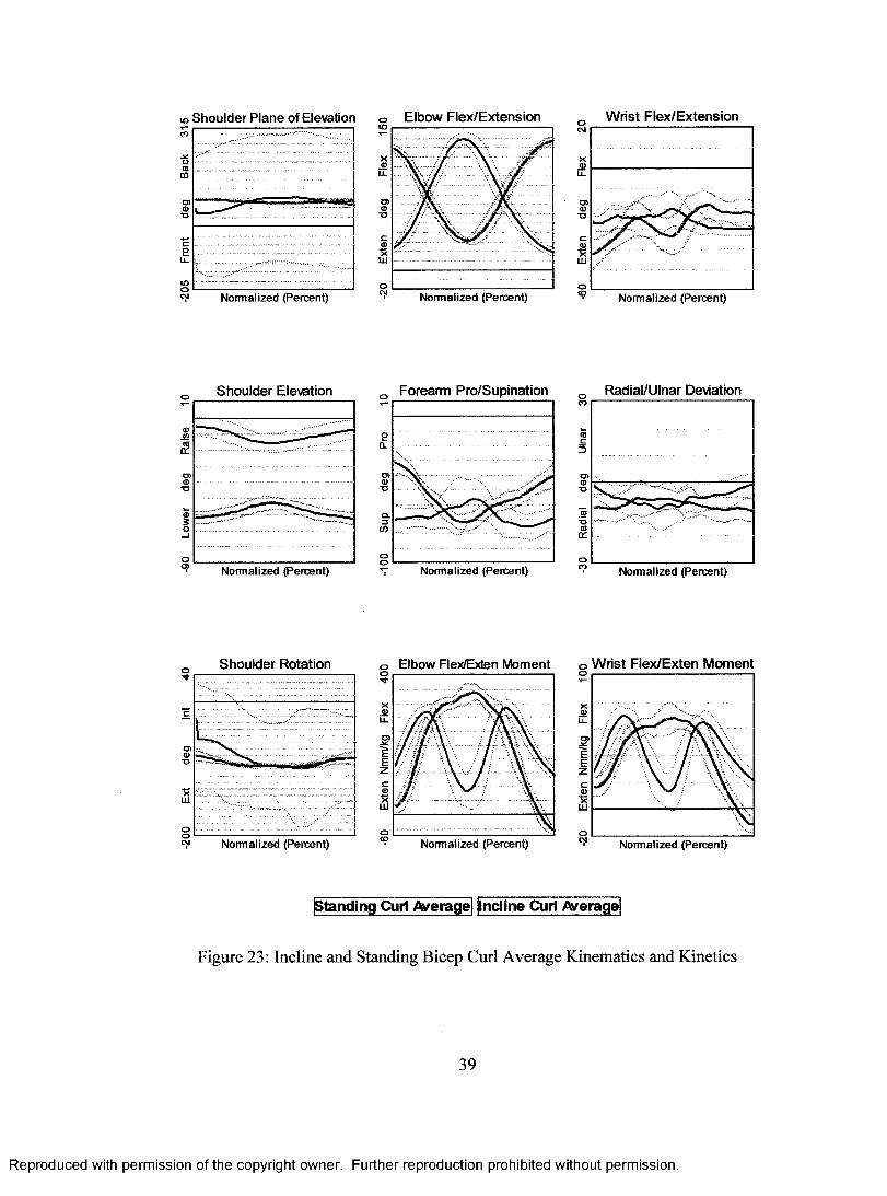
Figure 23 shows an example of bleep curl kinematics and kinetics for a subject.
All data from the incline and standing curls was time normalized, averaged, and plotted
together for comparison purposes. The solid green and red lines indicate the mean of the
data, while the dashed lines surrounding these lines indicate the standard deviation of the
data. The data is grouped into three columns: one for the shoulder, one for the elbow,
and another for the wrist.
The three graphs in the leftmost column are kinematic data for the shoulder. The
top graph shows the plane of elevation for the shoulder. Note that for the standing curl
the standard deviation of this plot is very large. The middle graph shows the elevation of
the shoulder. As expected, the upper arm is more elevated during the incline bicep curl.
Finally, the bottom graph shows the rotation of the upper arm. Again, note that the
standard deviation of the standing curl data is very large.
The center colunrn of graphs is relevant to the elbow joint. The top graph indicates
flexion/extension of the elbow throughout the bleep curl motion. The graph indicates that
during the standing curl the subject started and finished with their elbow extended, but
during the incline curl the subject started and finished with their elbow flexed. This was
consistent among all subjects and was done because it is the natural tendency to start and
finish in the most relaxed position. The middle graph in the center column represents
forearm pronation/supination. As expected, the forearm remains in a supinated position
throughout each exercise. Finally, the bottom graph is a plot of elbow flexion moment.
37
Reproduced with permission of the copyright owner. Further reproduction prohibited without permission.
Note that the flexion moment during the standing curl has two maxima, while the incline
curl only has one maximum.
The rightmost column of data represents kinematic and kinetic data for the wrist.
The top graph shows flexion/extension, the center graph shows radial/ulnar deviation,
and the bottom graph shows the flexion/extension moment. Note that the general shape
of the flexion/extension moment mimics that of the elbow flexion/extension moment.
38
Reproduced with permission of the copyright owner. Further reproduction prohibited without permission.
lo S hou lder P lan e of Elevation
LL
ONormalized (Percent)
E lbow F lex /E x ten sio nS
«u_
o>0)■O
oNormalized (Percent)
W rist F lex /E x ten sio n
LL
oNotmalized (Percent)
S h o u ld e r Elevation F orearm P ro /S up ina tion
Normalized (Percent)
20.
S’TO
oo
Normalized (Percent)
R adial/U lnar DeviationCO
Normalized (Percent)
S h o u ld e r R otation Elbow Flex/Exten M oment
X3
ONormalized (Percent) Normalized (Percent)
W rist F lex /E x ten M om entO
LL
Normalized (Percent)
standing Curl A/erage| incline Curl A/eragej
Figure 23; Incline and Standing Bicep Curl Average Kinematics and Kinetics
39
Reproduced with permission of the copyright owner. Further reproduction prohibited without permission.
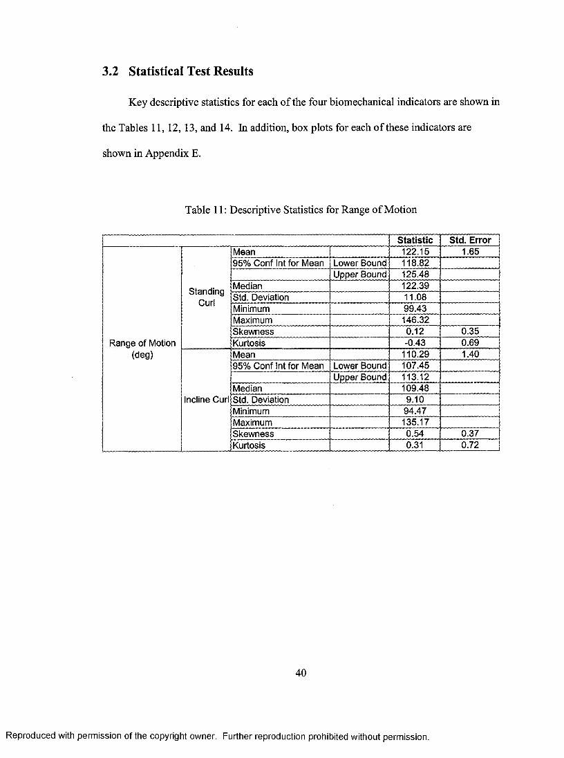
3.2 Statistical Test Results
Key descriptive statistics for each of the four biomechanical indicators are shown in
the Tables 11, 12, 13, and 14. In addition, box plots for each of these indicators are
shown in Appendix E.
Table 11 : Descriptive Statistics for Range of Motion
Statistic Std. ErrorM ean 1 2 2 .1 5 1 .659 5 % C o n f Int fo r M ean L ow er B ound 118 .8 2
U p p e r B ound 125 .4 8
S ta n d in gCurl
M edian 1 2 2 .3 9S td . D eviation 1 1 .0 8M inimum 9 9 .4 3M axim um 146 .3 2S k e w n e s s 0 .1 2 0 .3 5
R a n g e o f M otion K urtosis -0 .4 3 0 .6 9(d eg ) M ean 110 .2 9 1 .40
9 5 % C o n f Int fo r M ean L ow er B ound 1 0 7 .4 5U p p e r B ound 113 .1 2
M edian 1 0 9 .4 8Incline Curl S td . D eviation 9 .1 0
M inimum 9 4 .4 7M axim um 135 .1 7S k e w n e s s 0 .5 4 0 .3 7K urtosis 0.31 0 .7 2
40
Reproduced with permission of the copyright owner. Further reproduction prohibited without permission.

Table 12: Descriptive Statistics for Maximum Flexion Moment
Statistic Std. ErrorM ean 3 1 2 .2 9 5 .5 59 5 % C o n f Int fo r M ean L ow er B ound 3 0 1 .1 2
U p p e r B ound 3 2 3 .4 7
S ta n d in gCurl
M edian 3 1 6 .4 2S td . D eviation 3 7 .2 0M inimum 2 4 8 .0 4M axim um 3 8 9 .2 5
M axim um Flexion S k e w n e s s 0 .0 6 0 .3 5K urtosis -1 .1 5 0 .6 9iviom em
(N m m /kg) M ean 3 5 6 .1 7 10 .509 5 % C o n f Int fo r M ean L ow er B ound 3 3 4 .9 5
U p p er B ound 3 7 7 .3 8M edian 3 6 0 .4 8
incline Curl S td . D eviation 6 8 .0 7M inim um 243 .81M axim um 4 8 8 .8 7S k e w n e s s -0 .0 2 0 .3 7K urtosis -0 .8 9 0 .7 2
Table 13: Descriptive Statistics for Flexion Angle at Maximum Moment
Statistic Std. ErrorM ean 7 1 .9 0 1.249 5 % C o n f Int fo r M ean L ow er B ound 6 9 .4 0
U p p er B ound 7 4 .3 9
S ta n d in gCurl
M edian 7 0 .6 2S td . D eviation 8 .3 0M inim um 5 3 .4 2M axim um 9 6 .7 6
Flexion A ngle a t M axim um M om en t
(d eg )
S k e w n e s s 0 .5 5 0 .3 5K urtosis 0 .6 5 0 .6 9M ean 3 5 .0 7 1 .5395% C o n f Int fo r M ean L ow er B ound 3 1 .9 9
U p p e r B ound 3 8 .1 6M edian 3 3 .9 0
Incline Curl S td . D eviation 9 .8 9M inimum 1 7 J 2M axim um 5 8 .4 7S k e w n e s s 0 .2 4 0 .3 7K urtosis -0 .4 9 0 .7 2
41
Reproduced with permission of the copyright owner. Further reproduction prohibited without permission.

Table 14: Descriptive Statistics for Mean Flexion Moment
Statistic Std. ErrorM ean 1 6 4 .8 7 4 .2 59 5 % C o n f Int fo r M ean L ow er B ound 156 .3 0
U p p e r B ound 1 7 3 .4 4
S ta n d in gCurl
M edian 1 6 5 .0 7S td . D eviation 28 .51M inimum 1 1 0 .2 9M axim um 2 2 8 .7 7
M ean F lexion M om en t
(N m m /kg)
S k e w n e s s -0 .0 6 0 .3 5K urtosis -0.51 0 .6 9M ean 181.21 4 .1 895 % C o n f Int fo r M ean L ow er B ound 172 .7 8
U p p e r B ound 189 .6 4M edian 188 .9 7
incline Curl S td . D eviation 2 7 .0 6M inimum 1 1 1 .8 4M axim um 215 .51S k e w n e s s -1 .3 3 0 .3 7K urtosis 1 .13 0 .7 2
Table 15 shows the results of independent samples t-tests for each biomechanical
indicator. Note that for each biomechanical indicator there is statistically significant
evidence to reject the null hypothesis. In other words, there is significant evidence to
conclude that there is a difference between the biomechanical indicators of the standing
and incline bicep curls. The data show that the range of motion is 11.9° less on average
for the incline curl. The maximum flexion moment is 43.9 Nmm/kg greater on average
for the incline bicep curl. The flexion angle at which the maximum flexion moment
occurs is 71.9° for the standing bicep curl and 35.1° for the incline bicep curl, a
difference of 36.8°. Finally, the mean flexion moment for the incline curl is 16.3
Nmm/kg greater than for the standing curl.
42
Reproduced with permission of the copyright owner. Further reproduction prohibited without permission.

Table 15: Independent Samples t-test for Equality of Means
Test Statistic DOF P-Vaiue (2-taiied) Mean DifferenceFlexion R a n g e of M otion (d eg ) 5 .4 7 8 3 .6 7 0 .0 0 11 .87
M axim um Flexion M om en t (N m m /kg) -3 .6 9 6 2 .5 2 0 .0 0 -4 3 .8 7
F lexion A ng le a t M axim um M om en t (d eg )
18 .74 8 0 .3 0 0 .0 0 3 6 .8 2
M ean F lexion M om en t (N m m /kg) -2 .7 4 8 4 .9 7 0.01 -1 6 .3 4
43
Reproduced with permission of the copyright owner. Further reproduction prohibited without permission.

4 Discussion
The results of this study indicate that there are key biomechanical differences
between standing and incline dumbbell bicep curls. Based on the results of this study one
could speculate that the incline bicep curl is the better of the two exercises. The
maximum and mean elbow flexion torque is greater for this exercise, indicating a higher
load on the elbow flexor muscles. Also, on average the maximum flexion moment of the
incline bicep curl occurs at an angle of 35.1° versus 71.9° for the standing bicep curl.
This difference stems from the elevation of the upper arm and has implications on the
loading of the elbow flexor muscles. Figure 24 shows how the moment arm of the elbow
flexor muscles changes throughout the range of motion of the elbow. At a flexion angle
of 90° the line of pull of the biceps is normal to the forearm, thus the ability to generate
torque is optimized. The maximum moment of the standing bicep curl occurs closer to
this optimum flexion angle, meaning that not only does the incline bicep curl have a
higher flexion moment, but the more inefficient moment arm of the biceps requires a
much greater contractile force.
44
Reproduced with permission of the copyright owner. Further reproduction prohibited without permission.

a. b. d.
Figure 24: Varying Moment Arm of Biceps [1]
4.1 Limitations
Understanding the limitations involved in biomechanical modeling is fundamental
to any study, especially with regard to upper extremity modeling. Disregarding
limitations can lead to incorrect interpretation of both kinematics and kinetics. For this
reason, a detailed explanation of the known limitations of the upper extremity model
developed in this study is in order.
The model developed in this study is a link-segment model. For example. Figure
25 shows a 2D link segment model for the lower limb. In the model, the body is broken
into separate segments, each of which is assigned mass and inertial properties based on
anthropometric measurements. In order to construct this model certain assumptions are
made about the body. Winter states five distinct assumptions pertaining to link-segment
modeling, all of which are applicable to this study^^l
45
Reproduced with permission of the copyright owner. Further reproduction prohibited without permission.

1. Each segment has a fixed mass point as its COM (which will
be the center of gravity in the vertical direction)
2. The location of each segment’s COM remains fixed during the
movement.
3. The joints are considered to be hinge (or ball and socket)
joints.
4. The mass moment of inertia of each segment about its COM is
constant during the movement.
5. The length of each segment remains constant during the
movement (e.g., the distance between hinge or ball and socket
joints remains constant)^^l
A n a l o m i c a lM o d e l
Link S e g m e n t M o d e l
Figure 25: Link Segment Model^^^
46
Reproduced with permission of the copyright owner. Further reproduction prohibited without permission.

Clearly, each of these assumptions is an approximation to simplify the modeling
process. First, muscular contraction, or any change in the distribution of mass in the
segment, changes the location of the segment’s COM and moment of inertia.
Furthermore, simply determining the location of the COM and the moment of inertia of
any segment is error prone. These properties cannot be directly measured. Instead,
cadaver studies have been conducted in which these properties were directly measured.
The outcome of the studies are in the form of tables that allow for any body segment’s
COM and inertial properties to be calculated based on measurements of total body mass
and segment length. Since no two individuals have exactly the same build these tables
only give an estimate of the true value. The tables would most accurately be applied to
an individual of the same age, gender, and body type as the subjects in the cadaver study.
Second, no joint in the human body acts as a perfect hinge or ball and socket joint.
All joints experience some translation during motion or deviate in some way from being a
perfect joint. For example, the knee joint is often thought of as a hinge joint. If this were
the case then the center of rotation would be a constant. However, the instantaneous
center of rotation follows a semicircular pattern throughout the range of motion. In
addition, the knee joint also undergoes small amounts of rotation in the frontal and
transverse planes. Again, this violates the assumption that the knee joint is a perfect
hinge joint. Similar consideration must be taken at all joints in the body. For example,
finding the center of rotation of the shoulder joint is based on the assumption that the
shoulder acts as a perfect ball and socket joint. However, in many patients there is
significant translation at the glenohumeral joint. Thus, care must be taken to only apply
this method to patients that do not have significant glenohumeral joint translation.
47
Reproduced with permission of the copyright owner. Further reproduction prohibited without permission.

Some limitations were unique to this study. For instance, the original method for
defining the center of mass of the hand segment was to use a marker placed on the center
of the third metacarpal. However, after the first attempt at data collection it became
apparent that marker occlusion would prevent the use of this method because the marker
was not visible to the motion capture cameras for the majority of the bicep curl motion.
To circumvent this problem a new method had to be developed to define the hand center.
Instead of using a marker placed on the hand, the midpoint of the two markers placed at
the end of the dumbbell was used. This seemed effective, but undoubtedly introduced
error into the data. There was no way of verifying that subject held the dumbbell such
that the center of the bar was directly in line with the hand center, nor was it possible to
accurately measure the distance between the midpoint of the dumbbell and the actual
hand center. In addition, the way in which the dumbbell is held in the hand slightly
changes throughout the motion of the bicep curl. The effect of this error would be
greatest on wrist joint kinematics and kinetics, but it would also have a small impact on
the kinematics and kinetics of the elbow and shoulder. For this reason it is not
recommended that the wrist joint kinematics generated during this study be used to draw
any clinical conclusions.
Error due to marker placement is often underestimated. At times it can be very
difficult to accurately palpate bony landmarks and place surface markers. For large
segments, such as the thorax, the effect of this error is reduced, but in some segments
marker placement error can have an enormous impact on the outcomes of the study. For
example, in this study the flexion/extension axis of the elbow was defined by two
markers placed on the medial and lateral epicondyles of the humerus. The distance
48
Reproduced with permission of the copyright owner. Further reproduction prohibited without permission.

between the markers is small, thus any error in marker plaeement results in a relatively
large change in the direction of the flexion axis of the elbow. Since both kinematics and
kinetics of the elbow are calculated using this axis, it is crucial to accurately place the
elbow markers. The ISB specifically addresses this issue and recommends an alternative
method for defining this axis. Their recommendation is to define the elbow flexion axis
as being perpendicular to the long axis of the humerus and the long axis of the forearm.
However, this researcher’s experience was that this method resulted in significant
artificial humeral rotation when the elbow was near straight. Similarly, the wrist joint
suffers the same problem since the flexion axis of the wrist is defined by two markers
placed on the ulnar and radial styloids. However, axis definition is not the only concern
associated with using surface markers.
Modeling of the shoulder joint is subject to debate on many levels. First, it can be
debated whether or not the location of the shoulder joint center can be accurately
represented using surface markers. However, studies have been performed specifically to
address this issue and have verified that surface based markers can accurately define the
shoulder joint eenter^^^l Nevertheless it is still necessary to determine what surface
markers will be used to accomplish this task. When a spherical joint center method is
used, the shoulder joint center can be located with respect to either the scapula or the
humerus coordinate systems, since by definition the location of the point should be
constant in both. Consider the ease in which the shoulder joint center is located in the
scapula coordinate system, as was done in the model developed in this study. Accurately
tracking the scapula using surface markers is nearly impossible, especially when there is
significant scapulothoracic motion. Significant scapulothoracic motion occurs when the
49
Reproduced with permission of the copyright owner. Further reproduction prohibited without permission.

humerus is elevated above horizontal. For this reason it is not recommended that the
model developed in this study be used for any overhead motions. Second, consider the
case in which the shoulder joint center is defined in the humerus coordinate system. This
requires that three non-collinear points be used to define the humerus. At least one of
these points must be located on a wand or a cuff placed on the upper arm because there
are only two palpable bony landmarks on the humerus. This method is used by many
upper extremity models^^l However, this is clearly subject to error because of the large
amount of soft tissue movement on the upper arm, especially with obese or muscular
subjects. Soft tissue movement results in changes in the direction of the defining axes of
the humeral coordinate system, thus changes in the location of the estimated shoulder
joint center. It is this researcher’s experience that using the scapula to define the shoulder
joint center is a more accurate method. This conclusion was drawn in the development
stages of this model by using both methods to define the shoulder joint center. The
distance between the acromion marker and the shoulder joint center was plotted for
various motions. This distance would ideally be constant, however, when the shoulder
joint center was defined in the humeral coordinate system there was significant variation
in the location of the shoulder joint center. Nevertheless, this is not the only issue with
modeling of the shoulder.
The way in which shoulder joint angles are calculated and represented is also
subject to debate. Shoulder joint angles are either represented using the traditional
flexion/extension, ab/adduction, and rotation method or using the globographic method
used in this study. The ISB specifically recommends the use of the globographic method,
however, based on the results of this study this researcher does not completely agree with
50
Reproduced with permission of the copyright owner. Further reproduction prohibited without permission.

the ISB’s recommendation. Refer to Figure 23 for an illustration of the shoulder joint
kinematics using the globographic method. Notice, for both curl variations there is an
excessive amount of external humerus rotation. In reality, there is very little or no
humeral rotation during a standing bicep curl. The artificial rotation shown in the data
stems from the Euler rotation sequence used to calculate the globographic rotation
sequence. As previously discussed, the rotation sequence chosen to calculate three
dimensional rotations has an impact on the individual rotation angles. Humeral rotation
is the last rotation in the globographic rotation sequence, thus it is greatly affected by the
previous two rotations in the sequence.
Another problem with the globographic method becomes apparent when the arm is
near vertical, such as during the standing bicep curl. The data show an extremely large
variation in both the shoulder plane of elevation and rotation. This variation occurs
because the upper arm is near vertical, thus small changes in the position of the arm result
in large changes in the plane of elevation. For example, if the arm is directly in front of
the body the plane of elevation is 90°. If the arm moves by a small amount such that it is
now directly behind the body the plane of elevation is 270°. This large variation in the
shoulder plane of elevation also explains the large variation in shoulder rotation, again
because of the sequence dependence of the angles.
The globographic approach of representing shoulder position only seems applicable
during movements in which the arm is abducted and elevated. This minimizes the effect
of sequence dependence in calculating the angles and eliminates the large variability in
the shoulder plane of elevation. Conversely, during motions in which the arm is not
abducted, such as walking or running, the traditional flexion/extension, ab/adduction, and
51
Reproduced with permission of the copyright owner. Further reproduction prohibited without permission.

rotation description method should be used. The ISB’s recommendation to only use the
globographic approach should be modified to include such a statement.
4.2 Recommendations
Based on the results of the study certain recommendations can be made pertaining to
future studies in upper extremity biomechanics. The model developed here was a first
attempt at upper extremity modeling, thus there is much room for improvement, both in
experimental methodology and modeling techniques.
First and most important, a great deal of emphasis must be placed on simultaneous
development of upper extremity models and experimental methods. The extremely
versatile function of the upper extremity necessitates that models be developed to
accommodate the motions they are intended to study. In this study the upper extremity
model was developed without consideration of the movement that was intended to be
studied. This caused a great deal of difficulty when it was time to collect data, mainly
because of unforeseen problems with marker occlusion. Both the incline bench and the
dumbbell blocked the markers from the view of the motion capture cameras. Better
preparation would have revealed these problems early on and would have allowed for a
different marker set to be developed for the model.
Second, it should be decided early on whether or not to use the globographic method
to represent shoulder joint angles. As revealed in this study, the globographic method has
limitations when the upper arm is near vertical or when the primary motion of the
shoulder is in the sagittal plane, such as in walking or running. In these cases the
alternative flexion/extension, ab/adduction method should be used. The globographic
52
Reproduced with permission of the copyright owner. Further reproduction prohibited without permission.

method is most applicable for motions such as throwing, where the arm is both elevated
and abducted.
Finally, the model developed in this study used a spherical method to estimate the
shoulder joint center. This method was employed because of its simplicity and because
of time limitations. Future models would be much more robust if the helical axes method
was used. Not only is this method more accurate, but it would also allow for accurate
determination of the direction of the flexion axis of the elbow and wrist. This was
undoubtedly a major source of error in the model developed in this study.
53
Reproduced with permission of the copyright owner. Further reproduction prohibited without permission.

5 Conclusion
An upper extremity model was developed and implemented in the study of two
variations of the bicep curl, a common strength training exercise. Four key
biomechanical indicator variables were investigated: range of motion for the elbow,
maximum elbow flexion moment, mean elbow flexion moment, and the flexion angle at
which the maximum flexion moment occurs. On average, the range of motion was 11.9°
less for the incline curl. The maximum flexion moment was 43.9 Nmm/kg greater for the
incline bicep curl. The flexion angle at which the maximum flexion moment occurs was
71.9° for the standing bicep curl and 35.1° for the incline bicep curl, a difference of
36.8°. Finally, the mean flexion moment for the incline curl was 16.3 Nmm/kg greater
than for the standing curl.
54
Reproduced with permission of the copyright owner. Further reproduction prohibited without permission.

6 References
1. Nordin, M. and V.H. Frankel, Basic Biomechanics o f the Musculoskeletal System. 3rd ed. 2001, Baltimore, MD: Lippincott Williams & Wilkins.
2. Hamilton, N. and K. Luttgens, Kinesiology: Scientific Basis o f Human Motion. 10th ed. 2002, New York, NY: McGraw-Hill.
3. Winter, D.A., Biomechanics and Motor Control o f Human Movement. Third ed. 2005, Hoboken, New Jersey: John Wiley & Sons, Inc.
4. Soutas-Little, R.W. and D.J. Inman, Engineering Mechanics Dynamics. 1999, Upper Saddle River, New Jersey: Prentice Hall.
5. Grood, E.S. and W.J. Suntay, A joint coordinate system fo r the clinical description o f three-dimensional motions: application to the knee. J Biomech Eng, 1983.105(2): p. 136-44.
6. van der Helm, F.C. and G.M. Pronk, Three-dimensional recording and description o f motions o f the shoulder mechanism. J Biomech Eng, 1995.117(1): p. 27-40.
7. Williams, S., et al.. An upper body model fo r the kinematical analysis o f the joint chain o f the human arm. J Biomech, 2006. 39(13): p. 2419-29.
8. Wu, G., et al., ISB recommendation on definitions o f joint coordinate systems o f various joints fo r the reporting o f human joint motion—Part II: shoulder, elbow, wrist and hand. J Biomech, 2005. 38(5): p. 981-992.
9. Reid, T.A. (1994). Three-Dimensional Dynamic Motion of the Shoulder Complex. MS Thesis, Michigan State University.
10. Schmidt, R., et al., A marker-based measurement procedure fo r unconstrained wrist and elbow motions. J Biomech, 1999. 32(6): p. 615-21.
11. Meskers, C.G., et al.. In vivo estimation o f the glenohumeral joint rotation center from scapular bony landmarks by linear regression. J Biomech, 1998. 31(1): p. 93-6.
12. Veeger, HE., The position o f the rotation center o f the glenohumeral joint. J Biomech, 2000. 33(12): p. 1711-5.
13. Ehrig, R.M., et al., A survey offormal methods fo r determining the centre o f rotation o f ball joints. J Biomech, 2006. 39(15): p. 2798-809.
55
Reproduced with permission of the copyright owner. Further reproduction prohibited without permission.

14. Halvorsen, K., Bias compensated least squares estimate o f the center o f rotation.J Biomech, 2003. 36(7): p. 999-1008.
15. Stokdijk, M., J. Nagels, and P.M. Rozing, The glenohumeral joint rotation centre in vivo. J Biomech, 2000. 33(12): p. 1629-36.
16. Davids, J.R., Quantitative gait analysis in the treatment o f children with cerebral palsy. J Pediatr Orthop, 2006. 26(4): p. 557-9.
17. Ran, G., C. Disselhorst-Klug, and R. Schmidt, Movement biomechanics goes upwards: from the leg to the arm. J Biomech, 2000. 33(10): p. 1207-16.
18. Sibella, F. A new biomechanical model and experimental protocol fo r upper limbs movement analysis: validation... " in 7th Int. Symposium on 3D Analysis o f Human Movement. 2002. Newcastle upon Tyne, England.
19. Bahamonde, R.E. and D. Knudson, Kinetics o f the upper extremity in the open and square stance tennis forehand. J Sci Med Sport, 2003. 6(1): p. 88-101.
20. Dillman, C.J., G.S. Fleisig, and J.R. Andrews, Biomechanics o f pitching with emphasis upon shoulder kinematics. J Orthop Sports Phys Ther, 1993.18(2): p. 402-8.
21. Egret, C.I., et al.. Analysis o f 3D kinematics concerning three different clubs in go lf swing. Int J Sports Med, 2003. 24(6): p. 465-70.
22. Lloyd, D.G., J. Alderson, and B.C. Elliott, An upper limb kinematic model fo r the examination o f cricket bowling: a case study ofMutiah Muralitharan. J Sports Sci, 2000.18(12): p. 975-82.
23. Cote, J.N., et al.. Differences in multi-joint kinematic patterns o f repetitive hammering in healthy, fatigued and shoulder-injured individuals. Clin Biomech (Bristol, Avon), 2005. 20(6): p. 581-90.
56
Reproduced with permission of the copyright owner. Further reproduction prohibited without permission.

Appendix A: Center of Rotation Calculation
Calculation of the Center of Rotation (CoR) for the shoulder joint was done using a
least squares optimization. The total geometrie error, egeom, for m markers and n frames
of data is a function of the position of the CoR and the radius on whieh marker j travels,
rj. The position of marker j at frame i is denoted as pp.
^geom {CoR, 0 ) = Ê É - Pj. II - ( l a )j= l i= l
For any given marker at any given time the random error, e, ean be written as
ey [CoR, rj ) = ^{CoR - pj. ) • {CoR - » 0 (2a)
Taking the partial derivative of equation 2a yields a non-linear system o f m x n equations.
de-- 1 1 — = , {CoR - P a ) = — (CoR - P y )dCoR ^ ( C o R - p p ) * ( C o R - p p ) " r,,
dr [O j ^k ]
Where:
(3a)
rji = ^(CoR - Pji) • (CoR - pji)
~ - \ j ( ^ C o R ~ ^ J i ) ( y C o R ~ y j i ) (^ C o R ~ ^ j i )
(4a)
57
Reproduced with permission of the copyright owner. Further reproduction prohibited without permission.

Therefore, the Jacobian matrix for the system ean then be written as
J{CoR) =
CoR -11 Tcofl Til CoR 11ni 11
CoR ~ 11 y CoR ~ Til CoR ~ 11r- fa r,..j> J! JI
CoR ~ 11 CoR ~ 11 CoR ~ 11rmn rmn
-1
0
0 . 0
■1 . 0
0 . -1
(5a)
Newton’s method involves iterations consisting of five steps. Initial estimates of CoR
and Vj must be provided. The first step is to calculate an error matrix, E, for values from
the previous iteration, k-1.
(6a)
The second step is to calculate the Jacobian matrix using equation 5 a.
■CoR -11 T^],'^-Tii CoR 11'ii 11 'il
C R ~ 11 Tct« - Til CoR 11Ji Ji O'-
■CoR -*11 Tcofl 11 CoR 11rmn rmn rmn
-1 0 0
0 -1 0
0 0 -1
(7a)
58
Reproduced with permission of the copyright owner. Further reproduction prohibited without permission.
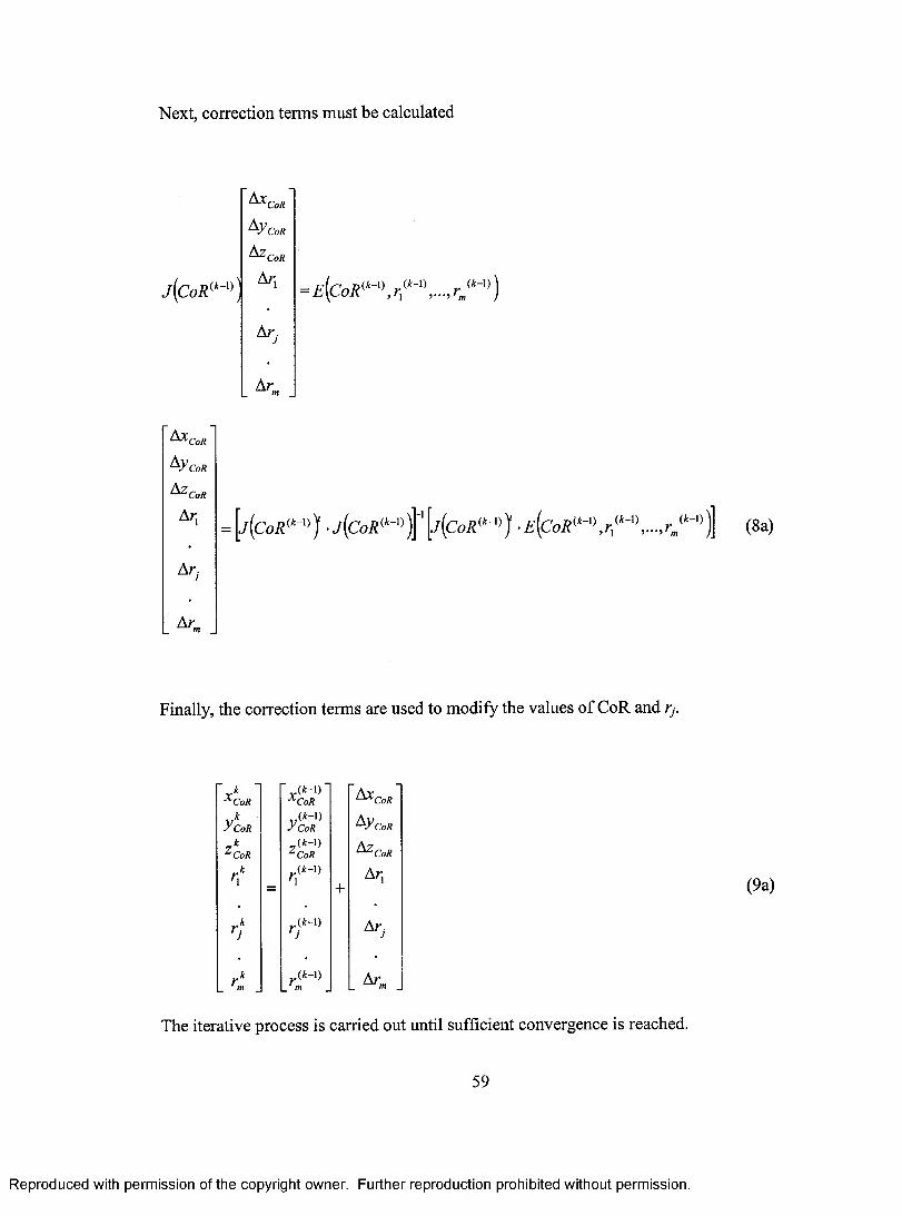
Next, correction terms must be calculated
j[CoR (i-i)
^CoRAy CoS^CoR
Ari
Ar
^CoRAy CoS^ C o R
Ar,
Ac
(8a)
Finally, the correction terms are used to modify the values of CoR and rj.
^ C o R" y ( t - l ) '
■^CoR ^ C o R
y CoR y ^ s ^ A y c b s
4 ._(*-!)^ C o R ^ C o R
n ' = ' \+
A n
r ( t - hV
A t j
. ^ 4„(* -!)
. m . ^ n . .
The iterative process is carried out until sufficient convergence is reached.
59
(9a)
Reproduced with permission of the copyright owner. Further reproduction prohibited without permission.

Appendix B: Vicon BodyLanguage Code
{*V IC O N B o d y L a n g u a g e ( tm ) m o d e l * }
{ * M o d e l U p p e r B o d y .M O D * }{ * U s e o n l y w i t h B o d y B u i l d e r V . 3 . 5 3 o r l a t e r * }( * U s e o n l y w i t h U p p e r B o d y .M P p a r a m e t e r s a n d U p p e r B o d y . MKR*}
{ * T h e m o d e l c a l c u l a t e s r i g h t s i d e d u p p e r b o d y k i n e m a t i c s a n d k i n e t i c s * }
{ * S t a r t o f m a c r o s e c t i o n * }{ * = = = = = = = = = = = = = = = = = = = = = = * }{ * = = = = = = = = = = = = = = = = = = = . = = * }
{ * T h i s m a c r o w i l l c a l c u l a t e t h r e e v e c t o r s r e p r e s e n t i n g t h e t h r e e l i n e s o f t h e 3 x 3 r o t a t i o n m a t r i x b a s e do n t h e XYZ f i x e d a x i s B o d y B u i l d e r d e f a u l t o u t p u t ( c h i l d , p a r e n t , X Y Z ) .I t w i l l t h e n u s e t h e s e l i n e s t or e c a l c u l a t e t h e t h r e e a n g l e s a l p h a , b e t a a n d gamma w h i c h r e p r e s e n t t h e r o t a t i o n s o b t a i n e d f o r t h e Y - X - Y a x i so r d e r e d d e c o m p o s i t i o n o f t h e r o t a t i o n m a t r i x . T h e m a c r o i s c a l l e d u s i n g :R o t Y X Y ( c h i l d s e g m e n t , p a r e n t s e g m e n t , j o i n t n a m e )( e . g . R o t Y X Y ( R i g h t U p p e r L e g , P e l v i s , H I P ) )
T h e l a b e l s j o i n t n a m e Y X Y e t c . ( e . g . HIPYXY) m u s t b e a d d e d t o t h e m a r k e r f i l e u s e d . * }
m a c r o R o t Y X Y ( c h i l d , p a r e n t , j o i n t ) j o i n t # a n g l e s = < c h i l d , p a r e n t , x y z > j o i n t # a l p h a = j o i n t # a n g l e s (1 ) j o i n t # b e t a = j o i n t # a n g l e s (2 ) j o i n t # g a m m a = j o i n t # a n g l e s (3 )
j o i n t # R x y z l = { c o s ( j o i n t # g a m m a ) * c o s ( j o i n t # b e t a ) , s i n ( j o i n t # g a m m a ) * c o s ( j o i n t # b e t a ) , - s i n ( j o i n t t t b e t a ) }j o i n t # R x y z 2 = { c o s ( j o i n t # g a m m a ) * s i n ( j o i n t # b e t a ) * s i n ( j o i n t # a l p h a ) - s i n ( j o i n t # g a m m a ) * c o s ( j o i n t # a l p h a ) , s i n ( j o i n t # g a m m a ) * s i n ( j o i n t # b e t a ) * s i n ( j o i n t # a l p h a ) + c o s ( j o i n t # g a m m a ) * c o s ( j o i n t # a l p h a ) , c o s ( j o i n t # b e t a ) * s i n ( j o i n t t t a l p h a ) }j o i n t # R x y z 3 = { c o s ( j o i n t # g a m m a ) * s i n ( j o i n t # b e t a ) * c o s ( j o i n t # a l p h a ) + s i n ( j o i n t # g a m m a ) * s i n ( j o i n t # a l p h a ) , s i n ( j o i n t # g a m m a ) * s i n ( j o i n t # b e t a ) * c o s ( j o i n t # a l p h a ) - c o s ( j o i n t # g a m m a ) * s i n ( j o i n t # a l p h a ) , c o s ( j o i n t # b e t a ) * c o s ( j o i n t # a I p h a ) }
b e t a = a c o s ( j o i n t # R x y z 2 ( 2 ) )I F b e t a > 0
b e t a = - b e t aEND I F
c a l p h a = j o i n t # R x y z 2 ( 3 ) / s i n ( b e t a ) s a l p h a = j o i n t # R x y z 2 ( 1 ) / s i n ( b e t a )
60
Reproduced with permission of the copyright owner. Further reproduction prohibited without permission.

alpha = atan2(salpha,calpha)
cgam m a = - j o i n t # R x y z 3 ( 2 ) / s i n ( b e t a ) sg a m m a = j o i n t # R x y z l ( 2 ) / s i n ( b e t a ) gam m a= a t a n 2 ( s g a m m a , c g a m m a )
I F ( b e t a < 0 . 5 AND b e t a > - 0 . 5 ) { * I f t h e e l e v a t i o n i s n e a r z e r o , s e tt h e t h i r d t o z e r o a n d s u p p o s e t h e m o v e m e n t h a s o n l y o n e c o m p * }
gamm a = a c o s ( j o i n t # R x y z 3 ( 3 ) ) a l p h a = 0
END I F
j o i n t # Y X Y = c a l p h a , b e t a , gamma>
o u t p u t ( j o i n t # Y X Y )
e n d m a c r o
M a c r o R E P L A C E 4 ( p l , p 2 , p 3 , p 4 ){ ♦ R e p l a c e s a n y p o i n t m i s s i n g f r o m s e t o f f o u r f i x e d i n a s e g m e n t * } s 2 3 4 = [ p 3 , p 2 - p 3 , p 3 - p 4 ] { * D e f i n e s a s e g m e n t s 2 3 4 u s i n g a l l p o i n t se x c e p t p i * }p l V = A v e r a g e ( p l / s 2 3 4 ) * s 2 3 4 ( * F i n d s t h e a v e r a g e p o s i t i o n o f p i i n t h e s 2 3 4 l o c a l C o - o r d s y s t e m a n d c r e a t e s v i r t u a l p o i n t p l V f r o m t h i s r e f e r e n c e s y s t e m * }s 3 4 1 = [ p 4 , p 3 - p 4 , p 4 - p l ] ( * D e f i n e s a s e g m e n t s 3 4 1 u s i n g a l l p o i n t se x c e p t p 2 * }p 2 V = A v e r a g e ( p 2 / s 3 4 1 ) * s 3 4 1 ( * F i n d s t h e a v e r a g e p o s i t i o n o f p 2 i n t h e s 3 4 1 l o c a l C o - o r d s y s t e m a n d c r e a t e s v i r t u a l p o i n t p 2 V f r o m t h i s r e f e r e n c e s y s t e m * }s 4 1 2 = [ p l , p 4 - p l , p l - p 2 ] ( * D e f i n e s a s e g m e n t s 4 1 2 u s i n g a l l p o i n t se x c e p t p 3 * }p 3 V = A v e r a g e ( p 3 / s 4 1 2 ) * s 4 1 2 { * F i n d s t h e a v e r a g e p o s i t i o n o f p 3 i n t h e s 4 1 2 l o c a l C o - o r d s y s t e m a n d c r e a t e s v i r t u a l p o i n t p 3 V f r o m t h i s r e f e r e n c e s y s t e m * }s l 2 3 = [ p 2 , p l - p 2 , p 2 - p 3 ] { * D e f i n e s a s e g m e n t s l 2 3 u s i n g a l l p o i n t se x c e p t p 4 * }p 4 V = A v e r a g e ( p 4 / s l 2 3 ) * s l 2 3 ( * F i n d s t h e a v e r a g e p o s i t i o n o f p 4 i n t h es l 2 3 l o c a l C o - o r d s y s t e m a n d c r e a t e s v i r t u a l p o i n t p 4 V f r o m t h i s r e f e r e n c e s y s t e m * }{ * Now o n l y r e p l a c e s i f o r i g i n a l i s m i s s i n g 1 1 - 9 9 * }p i = p i ? p l Vp 2 = p 2 ? p 2 Vp 3 = p 3 ? p 3 Vp 4 = p 4 ? p 4 Ve n d m a c r o
m a c r o R E P L A C E S ( p i , p 2 , p 3 , p 4 , p 5 ){ ♦ R e p l a c e s a n y p o i n t m i s s i n g f r o m s e t o f f i v e f i x e d i n a s e g m e n t * }
{♦S E C T IO N FOR IN I T I A L I S A T I O N OF VIRTUAL P O IN T S * }{♦R E P L A C E 4*}5 1 2 3 = [ p 2 , p l - p 2 , p 2 - p 3 ] p 4 V l = A v e r a g e ( p 4 / s l 2 3 ) * s l 2 35 1 2 4 = [ p 2 , p l - p 2 , p 2 - p 4 ] p 3 V l = A v e r a g e ( p 3 / s l 2 4 ) * s l 2 4 s l 3 4 = [ p 3 , p l - p 3 , p 3 - p 4 ]
61
Reproduced with permission of the copyright owner. Further reproduction prohibited without permission.

p 2 V l = A v e r a g e ( p 2 / s l 3 4 s 2 3 4 = [ p 3 , p 2 - p 3 , p 3 - p 4 p l V l = A v e r a g e ( p l / s 2 3 4
{ ♦ A d d i t i o n r e q u i r e d f o r REPLACES*}
* s l 2 3
* s l 2 4
s l 2 3 = [ p 2 , p l - p 2 , p 2 - p 3 p S V l = A v e r a g e ( p 5 / s l 2 3 S l 2 4 = [ p 2 , p l - p 2 , p 2 - p 4 p 5 V 2 = A v e r a g e ( p 5 / s l 2 4 s l 2 5 = [ p 2 , p l - p 2 , p 2 - p 5 p 3 V 2 = A v e r a g e ( p 3 / s 1 2 5 p 4 V 2 = A v e r a g e ( p 4 / s 1 2 5 s l 3 4 = [ p 3 , p l - p 3 , p 3 - p 4 p 5 V 3 = A v e r a g e ( p 5 / s l 3 4 s l 3 5 = [ p 3 , p l - p 3 , p 3 - p 5 p 2 V 2 = A v e r a g e ( p 2 / s 1 3 5 p 4 V 3 = A v e r a g e ( p 4 / s 1 3 5 s l 4 5 = [ p 4 , p l - p 4 , p 4 - p 5 p 2 V 3 = A v e r a g e ( p 2 / s 1 4 5 p 3 V 3 = A v e r a g e ( p 3 / s 1 4 5 S 2 3 4 = [ p 3 , p 2 - p 3 , p 3 - p 4 p 5 V 4 = A v e r a g e ( p 5 / s 2 34 s 2 3 5 = [ p 3 , p 2 - p 3 , p 3 - p 5 p l V 2 = A v e r a g e ( p l / s 2 3 5 p 4 V 4 = A v e r a g e ( p 4 / s 2 3 5 s 2 4 5 = [ p 4 , p 2 - p 4 , p 4 - p 5 p l V 3 = A v e r a g e ( p l / s 2 4 5 p 3 V 4 = A v e r a g e ( p 3 / s 2 4 5 s 3 4 5 = [ p 4 , p 3 - p 4 , p 4 - p 5 p l V 4 = A v e r a g e ( p i / s 3 4 5 p 2 V 4 = A v e r a g e ( p 2 / s 3 4 5
* s l 3 4
* S 2 3 4
* S 1 2 5* S 1 2 5
* S l 3 4
* S 1 3 5* 8 1 3 5
* 8 1 4 5* 8 1 4 5
* 8 2 3 4
* 8 2 3 5* 8 2 3 5
* 8 2 4 5* 8 2 4 5
* 8 3 4 5* 8 3 4 5
{♦SE C T IO N FOR S P E C IF IC A T IO N OF VIRTUAL P O IN T S *}p ip 2P3P3p 4P5
p ip 2P 3P 3p 4p 5
? p l V 2 ? p 2 V 2
p l V l p 2 V l p 3 V l ? p 3 V 2 p 3 V l ? p 3 V 2 p 4 V l ? p 4 V 2 p 5 V l ? p 5 V 2
? p l V 3 ? p 2V 3 ? p 3V 3 ? p 3V 3 ? p 4 V 3 ? p 5 V 3
? p l V 4 ? p 2 V 4 ? p 3 V 4 ? p 3 V 4 ? p 4 V 4 ? p 5 V 4
e n d m a c r o
M a c r o A X I S V I S U A L I S A T I O N ( S e g m e n t )0 R I G I N # S e g m e n t = 0 ( a e g m e n t )A X I S X # S e g m e n t = { 1 0 0 , 0 , 0 } * S e g m e n t A X I S Y # S e g m e n t = { 0 , 1 0 0 , 0 } * S e g m e n t A X I S Z # S e g m e n t = { 0 , 0 , 1 0 0 } * S e g m e n to u t p u t ( O R I G I N # S e g m e n t , A X I S X # S e g m e n t , A X I S Y # S e g m e n t , A X I S Z # S e g m e n t ) E n d m a c r o
{ ♦ E n d o f m a c r o Election*}{ * = = = = = = = = = = = = = = = = = = = = * }
{ ♦ I n i t i a l i a a t i o n a * }{ * = = = = = = = = = = = = = = = * }
{ * = = = = = = = = = = = = * }
{ * = = = = = = = = = = = = * }
62
Reproduced with permission of the copyright owner. Further reproduction prohibited without permission.

{ * S e t D e a d b a n d , e x c e p t f o r s t a t i c t r i a l s * }{ ♦ S e t t i n g t h e D e a d b a n d c a n h e l p a v o i d s e g m e n t a x i s f l i p * }
I f $ S t a t i c o l D e a d b a n d = $ D e a d b a n d E n d l f
( * S E T UP GLOBAL*}{ * = = = = = = = = = = = = = = = * }
G l o b a l = [ { 0 , 0 , 0 } , { 1 , 0 , 0 } , { 0 , 0 , 1 } , x y z ]GLOBO = { 0 , 0 , 0 }GLOBX = { 1 5 0 , 0 , 0 } * G l o b a l GLOBY = { O , 1 5 0 , 0 } * G l o b a l GLOBZ = { 0 , 0 , 1 5 0 } * G l o b a l OUTPUT(GLOBO,GLOBX,GLOBY,GLOBZ)
{♦SEGMENT D E F I N I T I O N S * }{* = = = = _ = = = = = = = = = *}{ * = = = = = = = = = = = = * }
{ * = = = = = = = = = = = = * }
{♦HEAD SEGMENT*}{*------= = = = = = = = *}R e p la c e 4 (L F H D ,R F H D ,R B H D ,L B H D )L H e a d = (L F H D +L B H D )/2 R H ea d = (R FH D +R B H D )/2 B H e a d = (L B H D +R B H D )/2 F H e a d = (L F H D + R F H D ) /2 ■H e a d = [ F H e a d , R H e a d - L H e a d , B H e a d - F H e a d , z y x ] A X IS V I S U A L I S A T I O N (H e a d )
{ * THORAX SEGMENT*}{ * = = = = = = = = = = = = = = * )
o p t i o n a l p o i n t s ( p x )
I f $ s t a t i c == 1D u m m y T h o r a x = [ C 7 , C 7 - T 8 , T 8 - 1 J , y z x ]$%VPX = P X /D u m m y T h o r a x 'Param ($% V P X )
E n d l f
I f $ s t a t i c <> 1I f e x i s t ( P X )
E l s eD u m m y T h o r a x = [ C 7 , C 7 - T 8 , T 8 - l J , y z x ] PX = $% VPX*Dum m yThorax o u t p u t ( P X )
E n d l fE n d l f
R e p l a c e 4 ( C 7 , T 8 , I J , P X )T R X 0 = 1 JB T h o r a x = ( T 8 + P X ) / 2 U T h o r a x = ( l J + C 7 ) / 2
63
Reproduced with permission of the copyright owner. Further reproduction prohibited without permission.

T h o r a x = [TRXO, U T h o r a x - B T h o r a x , I J - C 7 , y z x ] A X I S V I S U A L I S A T I O N ( T h o r a x )
{♦SCAPULA SEGMENT*}{ * = = = = = = = = = = = = = = * }
R e p l a c e 4 ( R A A , R A I , RAC,RPC)R S c a p u l a = [ R A A , R A A -R T S, R A A -R A I, z x y ] A X I S V I S U A L I S A T I O N ( R S c a p u la )
{♦ P O IN T S USED FOR GH CENTER CALCULATION*}{ * = = = = = = = = = = = = = = * }
scap R E M = R E M / R S c a p u l a s c a p R E L = R E L / R S c a p u l a o u t p u t ( s c a p R E M , s c a p R E L )
o p t i o n a l p o i n t s ( r w l , r w 2 , r f i n )
{♦HUMERUS D E F IN IT IO N USING OPTION 1 OF I S B * }{♦HUMERUS SEGMENT*}{ ♦ = = = = = = = = = = = = = = ♦ }
REJC = (R E L +R E M )/2R e p l a c e s ( R E J C , R U S ,R R S , R W 1 , R W 2 )RWJC = (R R S + R U S ) /2 o u t p u t (RWJC) o u t p u t (REJC)
R S J C = $ R S h o u l d e r J C * R S c a p u l a o u t p u t (R SJC)R e p l a c e 4 ( R E J C , REM, REL, RSJC)R H u m e ru s = [R S J C , R S J C -R E J C , REM-REL, y x z ] A X IS V IS U A L IS A T I O N (R H u m e r u s )
{♦ HUMERUS D E F IN IT IO N USING OPTION 2 , n o t u s e d h e r e * }
{*{ * HUMERUS SEGMENT*}{ * = = = = = = = = = = = = = = * }
REJC = (R E L +R E M )/2R e p l a c e s ( R E J C , R U S , R R S , R W l, RW2)RWJC = (R R S + R U S ) /2 o u t p u t (RWJC) o u t p u t (REJC)R S J C = $ R S h o u l d e r J C * R S c a p u l a o u t p u t (R SJC )R H u m e ru s = [R S J C , R S J C -R E J C , RW JC-REJC, y z x ] A X I S V I S U A L I S A T I O N ( R H u m e r u s ) *}
{♦FOREARM SEGMENT*}{ * = = = = = = = = = = = = = = * }
R F o r e a r m = [RWJC, REJC-RW JC, R U S -R R S , y x z ] A X IS V I S U A L I S A T I O N (R F o r e a r m ) humRW JC=RW JC/RHumerus o u t p u t (humRWJC)
{♦HAND SEGMENT AS DEFINED USING DUMBBELL M ID POIN T*}{ * = = = = = = = = = = = = = = * }
{♦DUMMY HAND SEGMENT*}
64
Reproduced with permission of the copyright owner. Further reproduction prohibited without permission.
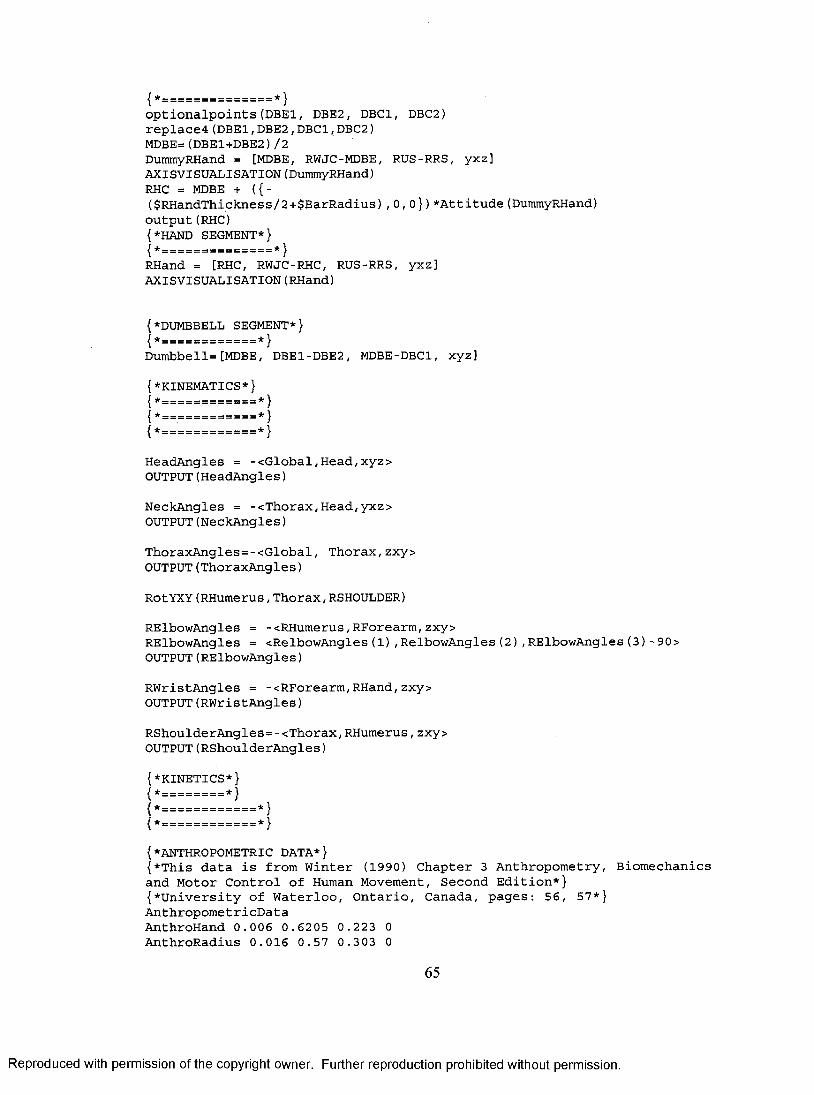
{ * = = = = = = = = — = = * }
o p t i o n a l p o i n t s ( D B E l , D B E 2 , D B C l , DBC2) r e p l a c e 4 ( D B E l , D B E 2 , D B C l , D BC 2)M D B E = (D B E 1 + D B E 2 ) /2DummyRHand = [MDBE, RWJC-MDBE, R U S -R R S , y x z ] A X IS V ISU A L IS A T IO N (D u m m yR H an d )RHC = MDBE + ( { -( $ R H a n d T h i c k n e s s / 2 + $ B a r R a d i u s ) , 0 , o } ) * A t t i t u d e ( D u m m y R H a n d )
o u t p u t (RHC){*HAND SEGMENT*}
R H and = [RHC, RWJC-RHC, R U S -R R S , y x z ]A X IS V IS U A L IS A T IO N (R H a n d )
{*DUMBBELL SEGMENT*}
{* *}D u m b b e l l = [ M D B E , D B E 1 -D B E 2 , M D B E -D B C l, x y z ]
{*K IN E M A TIC S*}{ * = = = = = = = = = = = = * }{* = --------= = = = = = = *}{* = = ------- = = = = = = *}
H e a d A n g l e s = - < G l o b a l , H e a d , x y z >OUTPUT( H e a d A n g l e s )
N e c k A n g l e s = - < T h o r a x , H e a d , y x z >OUTPUT( N e c k A n g l e s )
T h o r a x A n g l e s = - < G l o b a l , T h o r a x , z x y >OUTPUT( T h o r a x A n g l e s )
R o tY X Y ( R H u m e r u s , T h orax ,R S H O U L D E R )
R E l b o w A n g l e s = - < R H u m e r u s , R F o r e a r m , z x y >R E l b o w A n g l e s = < R e l b o w A n g l e s ( 1 ) , R e l b o w A n g l e s ( 2 ) , R E l b o w A n g l e s ( 3 ) - 9 0 > OUTPUT( R E l b o w A n g l e s )
R W r i s t A n g l e s = - < R F o r e a r m , R H a n d , z x y >OUTPUT( R W r i s t A n g l e s )
R S h o u l d e r A n g l e s = - < T h o r a x , R H u m e r u s , z x y >OUTPUT( R S h o u l d e r A n g l e s )
{ * K I N E T I C S * }{ * = = = = = = = = * }{ * = = = = = = = = = = = = * }{ * = = = = = = = = = = = = * }
{ *ANTHROPOMETRIC DATA*}{ * T h i s d a t a i s f r o m W i n t e r ( 1 9 9 0 ) C h a p t e r 3 A n t h r o p o m e t r y , B i o m e c h a n i c s a n d M o t o r C o n t r o l o f Human M o v e m e n t , S e c o n d E d i t i o n * }{ * U n i v e r s i t y o f W a t e r l o o , O n t a r i o , C a n a d a , p a g e s : 5 6 , 5 7 * }A n t h r o p o m e t r i c D a t aA n t h r o H a n d 0 . 0 0 6 0 . 6 2 0 5 0 . 2 2 3 0A n t h r o R a d i u s 0 . 0 1 6 0 . 5 7 0 . 3 0 3 0
65
Reproduced with permission of the copyright owner. Further reproduction prohibited without permission.

A n t h r o H u m e r u s 0 . 0 2 8 0 . 5 6 4 0 . 3 2 2 0 A n t h r o T h o r a x 0 . 3 5 5 0 . 6 3 0 . 3 1 0 A n t h r o H e a d 0 . 0 8 1 0 . 5 2 0 . 4 9 5 0 E n d A n t h r o p o m e t r i c D a t a
$ % R H u m e r u s L e n g t h = D I S T ( R S J C ,R E J C )PARAM( $ % R H u m e r u s L e n g th )
$ % R F o r e a r m L e n g t h = D I S T ( R E J C ,R U S )P A R A M ($ % R F o r e a r m L e n g th )
T h o r a x = [ T h o r a x , A n t h r o T h o r a x ]
{ * s q u a r e r a d i u s o f g y r a t i o n : . 1 0 3 = . 3 2 2 * * 2 *}R H u m e r u s = [ R H u m e r u s , 0 . 0 2 8 * $ B o d y M a s s , { 0 , 0 . 4 3 6 * $ % R H u m e r u s L e n g t h , 0 } , $ % R H u m e r u s L e n g t h * $ % R H u m e r u s L e n g t h * { . 1 0 3 , 0 , . 1 0 3 } * 0 . 0 2 8 * $ B o d y M a s s ] R H u m e r u s = [ R H u m e r u s , T h o r a x , RSJC]
{ * s q u a r e r a d i u s o f g y r a t i o n : . 0 9 1 = . 3 0 3 * * 2 * }R F o r e a r m = [ R F o r e a r m , 0 . 0 1 6 * $ B o d y M a s s , { 0 , 0 . 5 7 0 * $ % R F o r e a r m L e n g t h , 0 } , $ % R H u m e r u s L e n g t h * $ % R H u m e r u s L e n g t h * { . 0 9 1 , 0 , . 0 9 1 } * 0 . 0 1 6 * $ B o d y M a s s ] R F o r e a r m = [ R F o r e a r m , R H u m e r u s , REJC]
{ * s q u a r e r a d i u s o f g y r a t i o n : . 0 8 8 = . 2 9 6 * * 2 * }R H a n d = [R H a n d , 0 . 0 0 6 * $ B o d y M a s s , { 0 , 0 , 0 } ,$ R H a n d L e n g t h * $ R H a n d L e n g t h * ( . 0 8 8 , 0 , . 0 8 8 } * 0 . 0 0 6 * $ B o d y M a s s ]R H a n d = [R H a n d , R F o r e a r m , RWJC]
{ * s q u a r e r a d i u s o f g y r a t i o n : . 0 8 8 = . 2 9 6 * * 2 * }D u m b b e 1 1 = [ D u m b b e l l , $ D B M a s s , { 0 , 0 , 0 } ,{ $ D B I n e r t L o n g , $ D B I n e r t T r a n s , $ D B I n e r t T r a n s } ]D u m b b e l l = [ D u m b b e l l , R H a n d , RHC]
{ * JO IN T FORCES * }
{ * = = = = = = = = * }
R W r i s t F o r c e = 1 (R E A C T IO N (R H a n d )) / $ B o d y M a s s R E l b o w F o r c e = 1 (R E A C T I O N (R F o r e a r m )) / $ B o d y M a s s R S h o u l d e r F o r c e = 1 (R E A C T I O N (R H u m e r u s ) ) / $ B o d y M a s s OUTPUT ( R S h o u l d e r F o r c e , R E l b o w F o r c e , R W r i S t F o r c e )
{ * JO IN T MOMENTS * }
{ * = = = = = = = = * }{ * = = = = = = = = * }R W r is t M o m e n t = 2 (R E A C T IO N (R H a n d )) / ( $ B o d y M a s s ) R E lb o w M o m e n t = 2 (R E A C T I O N (R F o r e a r m )) / ( $ B o d y M a s s ) R S h o u l d e r M o m e n t = 2 (R E A C T I O N (R H u m e r u s ) ) / ( $ B o d y M a s s ) OUTPUT ( R S h o u l d e r M o m e n t , R E l b o w M o m e n t , R W r is t M o m e n t )
{* J O IN T POWERS * }{ * = = = = = = = = * }
{ * = = = = = = = = * }R W r i s t P o w e r = P O W E R (R F orea rm , R H a n d ) / ( $ B o d y M a s s ) R E l b o w P o w e r = PO W E R (R H um erus, R F o r e a r m ) / ( $ B o d y M a s s ) R S h o u l d e r P o w e r = P O W E R ( T h o r a x ,R H u m e r u s ) / ( $ B o d y M a s s ) OUTPUT ( R S h o u l d e r P o w e r , R E l b o w P o w e r , R W r i s t P o w e r )
66
Reproduced with permission of the copyright owner. Further reproduction prohibited without permission.
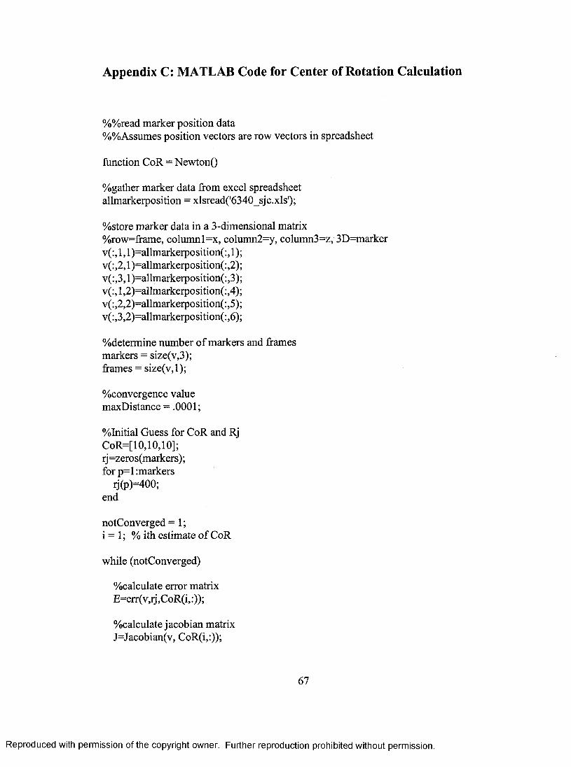
Appendix C: MATLAB Code for Center of Rotation Calculation
%%read marker position data%%Assumes position vectors are row vectors in spreadsheet
function CoR = NewtonQ
%gather marker data from excel spreadsheet allmarkerposition = xlsread('6340_sjc.xls');
%store marker data in a 3-dimensional matrix %row=frame, columnl=x, column2=y, column3=z, 3D=marker v(:, 1,1 )=allmarkerposition(:, 1); v(: ,2,1 )=allmarkerposition(: ,2) v(: ,3,1 )=allmarkerposition(: ,3) v(:, 1,2)=allmarkerposition(:,4) v( : ,2,2)=allmarkerposition( :, 5) v(:,3,2)=allmarkerposition(:,6)
%determine number of markers and frames markers = size(v,3); frames = size(v,l);
%convergence value maxDistance = .0001;
%Initial Guess for CoR and Rj CoR=[l 0,10,10]; ij=zeros(markers); for p=l markers
q(p)=400; end
notConverged = 1; i = 1; % ith estimate o f CoR
while (notConverged)
%calculate error matrix E=err(v,ij,CoR(i,:));
%calculate jacobian matrix J=Jacobian(v, CoR(i,:));
67
Reproduced with permission of the copyright owner. Further reproduction prohibited without permission.

%calculate change in CoR and Rj delta=inv( J'* J) * (J'* E) ;
%Detemiine New Values of CoR and Rj CoR=[CoR; CoR(i, :)+[delta( 1,1 ),delta(2,1 ),delta(3,1)]] ; for j= l markers
q(l,j)=ij(lj)+delta(3+j,l); end
%Determine if sufficient convergence reached if i >10000
disp('BC requires over 10000 iterations'); notConverged = 0;
end if(i> l)
if(norm( CoR(i,:)-CoR(i-l,:), inf) <= maxDistance ) % converged?notConverged = 0; % break from loop
end end
i = i+ 1; end
%Function to calculate error matrixfunction E=err(v, ij, CoR)xc=CoR(l);yc=CoR(2);zc=CoR(3);%%determine the number of fi-ames and markers present markers = size(v,3); frames = size(v,l);
E=zeros(markers*frames, 1);
for p=l markers for n=l : frames
ro w=((p-1 ) * frames+n) ; x=v(n,l,p); y=v(n,2,p); z=v(n,3,p);r=sqrt((xc-x)^2+(yc-y)'^2+(zc-z)^2);E(row,l)=-l*(r-ij(p));
endend
%Function to calculate Jacobian
68
Reproduced with permission of the copyright owner. Further reproduction prohibited without permission.

function Jacobian=Jacobian(v, CoR)xc=CoR(l);yc=CoR(2);zc=CoR(3);%%detennine the number of frames and markers present markers = size(v,3); frames = size(v,l);
Jacobian=zeros((markers*frames),(3+markers));
for p=l :markers for n=l: frames
xc=CoR(l); yc=CoR(2); zc=CoR(3); x=v(n,l,p); y=v(n,2,p); z=v(n,3,p);r=sqrt((xc-x)^2+(yc-y)^2+(zc-z)^2); row=((p-1 )*frames+n);J acobian(row, 1 )=(xc-x)/r ;Jacobian(row,2)=(yc-y)/r;Jacobian(row,3)=(zc-zyr;Jacobian(row,(3+p))=-1 ;
end end
69
Reproduced with permission of the copyright owner. Further reproduction prohibited without permission.
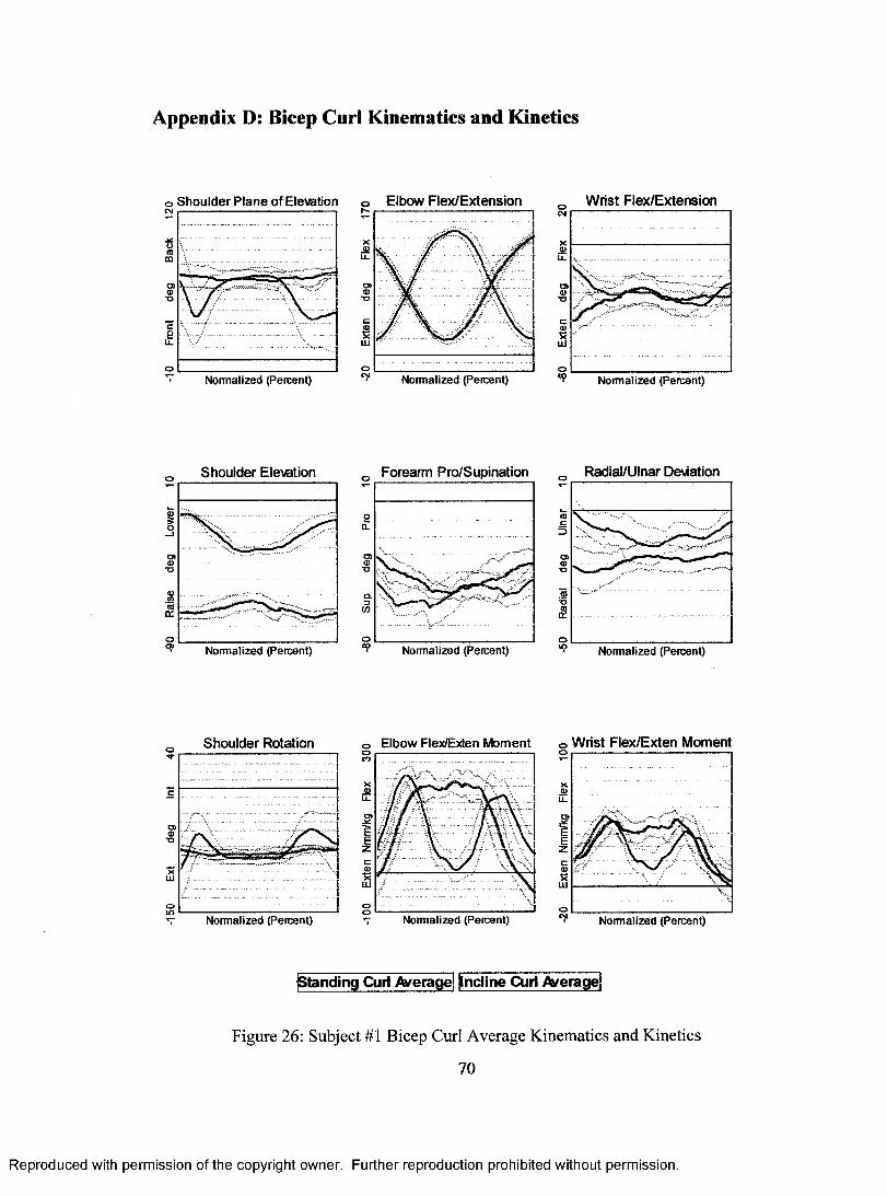
Appendix D: Bicep Curl Kinematics and Kinetics
Shoulder P lane of Elevation
U_
ONormalized (Percent)
E lbow F lex /E x ten sio n
11.
O)
ONormalized (Percent)
Wrist Flex/Extensions
u_
03
Normalized (Percent)
S h o u ld e r E levation
T3
ONormalized (Percent)
F orearm P ro /S up ination
T3
ONormalized (Percent)
g, R adial/U lnar Deviation
ONormalized (Percent)
S h o u ld er R otation
UJ
Normalized (Percent)
Elbow Flex/Exten M omentg
U_
oNomialized (Percent)
, W rist F lex /E x ten M om ent
U_
Normalized (Percent)
standing Curl A/eragel [Ecïïnië^üiril^
Figure 26: Subject #1 Bicep Curl Average Kinematics and Kinetics
70
Reproduced with permission of the copyright owner. Further reproduction prohibited without permission.

Shoulder Plane of Elevation Elbow Flex/Extension Wrist Flex/Extension
Normalized (Percent)
LL
"O
oNormalized (Percent)
■D
ONormalized (Percent)
S h o u ld e r Elevation
ONormalized (Percent)
F orearm P ro /S up ina tion
-a
oNormalized (Percent)
R adial/U lnar D e la tio n
oNonnallzed (Percent)
S h o u ld e r R otation
■o
Normalized (Percent)
Elbow Flex/Exten M oment
Li.
ONormalized (Percent)
W rist F lex /E x ten M om ent
Li.
a Nonnallzed (Percent)
Standing Curl Average Incline
Figure 27: Subject #2 Bicep Curl Average Kinematics and Kinetics
71
Reproduced with permission of the copyright owner. Further reproduction prohibited without permission.

. Shoulder Plane of Elevation Elbow Flex/ExtensionCM
Normallzecl (Percent)
IT)
u_
T3
Normalized (Percent)
Wrist Flex/ExtensionOCM
LL
Normalized (Percent)
S h o u ld e r E lexation
■a
Normalized (Percent)
F orearm P ro /S up ina tionO
2CL
O)(D■o
ONonnallzed (Percent)
R adial/U lnar Deviation
■u
ONomialized (Percent)
S h o u ld e r R otation
■o
Normalized (Percent)T
Elbow Flex/Exten M om ent
U -
lONormalized (Percent)
, W ris t F lex /E x ten M om entCM
U_
oNormalized (Percent)
standing Curi /Wetage] Incline Curi Average]
Figure 28: Subject #3 Bicep Curl Average Kinematics and Kinetics
72
Reproduced with permission of the copyright owner. Further reproduction prohibited without permission.

Shoulder Plane of ElevationCM
U.
O)
ONormalized (Percent)
E lbow F lex /E x ten s io nCO
■D
Nonnallzed (Percent)
W rist F lex /E x ten sio n
oNonnallzed (Percent)
Shoulder Elevation
Oq> Normalized (Percent)
Forearm Pro/Supination
oo
Normalized (Percent)
R adial/U lnar DeviationoCM
I
1a:o
Nonnallzed (Percent)
S h o u ld e r R otation Elbow Flex/Exten MomentO
o><DT3
soIf)
Normalized (Percent)
LL
Normalized (Percent)
W rist F lex /E x ten M om ent
LL
ONonnallzed (Percent)
standing Curl A/eraige]
Figure 29: Subject #4 Bicep Curl Average Kinematics and Kinetics
73
Reproduced with permission of the copyright owner. Further reproduction prohibited without permission.
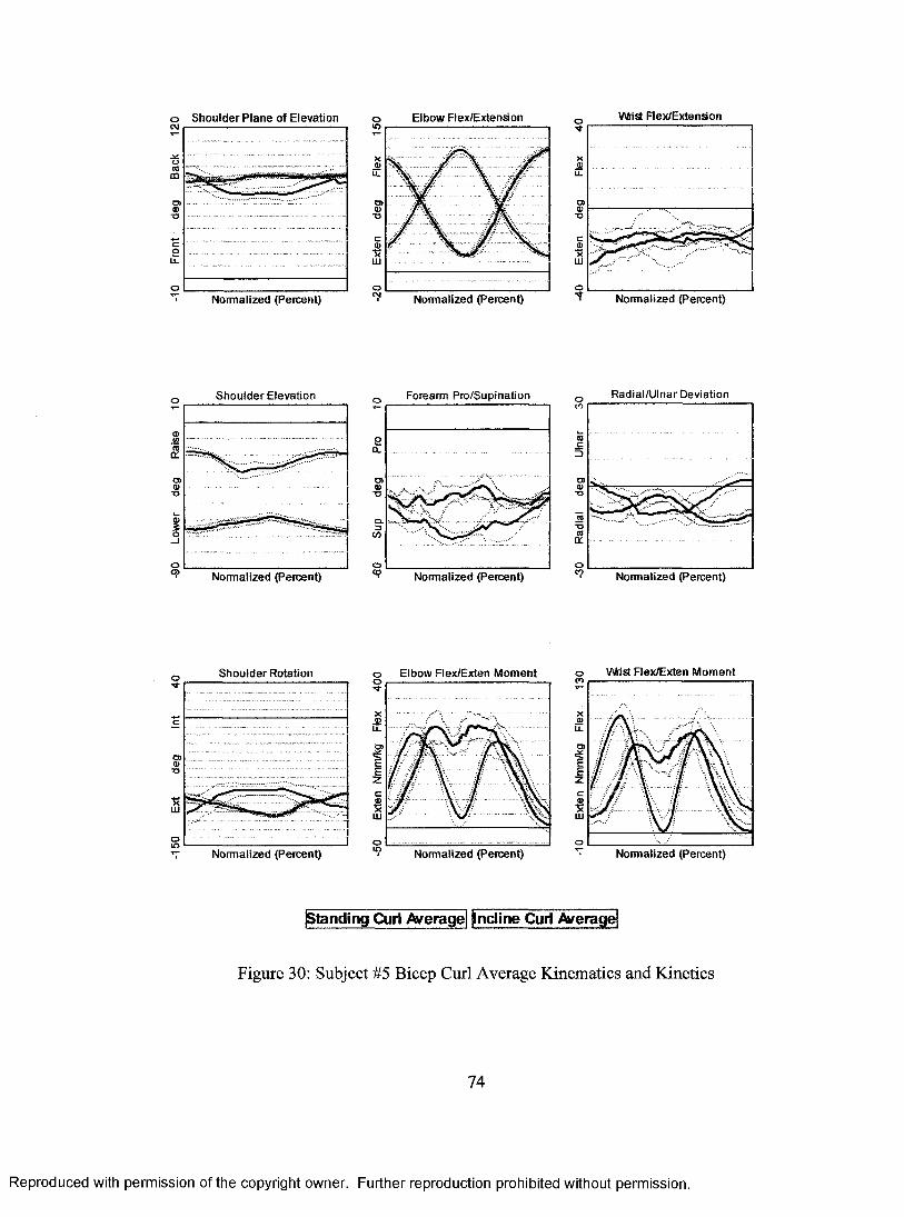
Shoulder P lane of Elevation Elbow Flex/Extension
u_
oNormalized (Percent)
u_
■o
Normalized (Percent)
VMM St Flex/Extensiono
u_
oNonnallzed (Percent)
Shoulder Elevation Forearm Pro/Suplnatlon
o>
I_i
? Normalized (Percent)o
Normalized (Percent)
Radial/Ulnar DeviationoCO
I
Ii
Io? Nofmalized (Percent)
Shoulder Rotation
■o
o
Nomialized (Percent)
Elbow Flex/Exten M omentI
I
IIS Normalized (Percent)
W ist Flex/Exten Moment
I
I
IO
Nomialized (Percent)
standing Curl Ai/eragel incline C u f^^
Figure 30: Subject #5 Bicep Curl Average Kinematics and Kinetics
74
Reproduced with permission of the copyright owner. Further reproduction prohibited without permission.

Appendix £: Biomechanical Indicator Box Plots
140.00
130.00
o 120.00
110.00
100.00
sending Incline
Curl Type
Figure 31 : Elbow Flexion Range of Motion Box Plot
75
Reproduced with permission of the copyright owner. Further reproduction prohibited without permission.
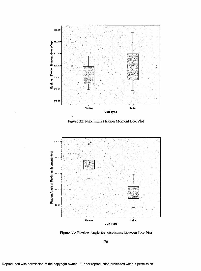
450.00
S i 400.00
350.00
300.00
250.00
200.00
Standing
Curl Type
Figure 32: Maximum Flexion Moment Box Plot
100.0 0 - 94
I80.00-
c
IoSE3E■|S»3)
<Cog
60 .00-
40 .00-
u.20 .00 -
Standing Incline
Curl Type
Figure 33: Flexion Angle for Maximum Moment Box Plot
76
Reproduced with permission of the copyright owner. Further reproduction prohibited without permission.

2 2 5 .0 0 -
Σ 200.0 0 -
175.00“
S 150 .0 0 -
125 .0 0 - 87 84
830
100 .0 0 -
Standing incline
Curi Type
Figure 34: Mean Flexion Moment Box Plot
77
Reproduced with permission of the copyright owner. Further reproduction prohibited without permission.