An Update on Brane Supersymmetry Breaking

J. Mourad a and A. Sagnotti b

aAPC, UMR 7164-CNRS, Universite Paris Diderot – Paris 710 rue Alice Domon et Leonie Duquet

75205 Paris Cedex 13 FRANCE

e-mail: mourad@apc.univ-paris7.fr

bScuola Normale Superiore and INFNPiazza dei Cavalieri, 7

56126 Pisa ITALY

e-mail: sagnotti@sns.it

Abstract

“Brane supersymmetry breaking” is a peculiar phenomenon that can occur in perturbativeorientifold vacua. It results from the simultaneous presence, in the vacuum, of non–mutuallyBPS sets of BPS branes and orientifolds, which leave behind a net tension and thus arunaway potential, but no tachyons. In the simplest ten–dimensional realization, the low–lying modes combine the closed sector of type–I supergravity with an open sector includingUSp(32) gauge bosons, fermions in the antisymmetric 495 and an additional singlet playingthe role of a goldstino. We review some properties of this system and of other non–tachyonicmodels in ten dimensions with broken supersymmetry, and we illustrate some puzzles thattheir very existence raises, together with some applications that they have stimulated.

Based in part on the lectures presented by A.S. at the“International School of Subnuclear Physics”, 55th Course, Erice, June 14 – 23 2017,

at TFI-2017, Parma, September 11 – 13 2017,and at LACES 2017, Firenze, November 27 – December 1, 2017

Dedicated to the memory of Yassen S. Stanev

arX

iv:1

711.

1149

4v1

[he

p-th

] 3

0 N

ov 2

017

1 Introduction

There are only a few ten–dimensional string models [1] without tachyonic excitations, andthey fall naturally into three classes, depending on the number of supersymmetries. Thefirst is widely familiar: it comprises the IIA and IIB models, whose low–lying modesbelong to the unique type–IIA (1, 1) and type–IIB (2, 0) supersymmetry multiplets, andwhose low–energy interactions are encoded in the corresponding versions of ten–dimensionalsupergravity [2]. Another class, which is equally familiar, comprises the two heterotic HEand HO models [3], with gauge groups E8×E8 and SO(32), and the type–I SO(32) (openand closed) superstring [4]. In these three cases, the low–lying modes fill the two availabletypes of (1, 0) supersymmetry multiplets, while the low–energy interactions are encoded inminimal supergravity coupled a la Green–Schwarz [4] to ten–dimensional supersymmetricYang–Mills theory. However, the three models are intrinsically different, since the SO(32)(open and closed) superstring provides the simplest example of an orientifold construc-tion [5], which links it to the type–IIB model. A third class of non–tachyonic modelsexists, however, which is the focus proper of this review. Supersymmetry is either absent intheir tachyon–free spectra or it is strikingly present in a non–linear phase, without an orderparameter capable of recovering it. The first model of this type is the SO(16) × SO(16)heterotic string of [6]: as we shall review shortly, its chiral spectrum obtains from thesupersymmetric HE model via an orbifold construction, in the spirit of [7]. The secondmodel descends via an orientifold construction [8] from a tachyonic and purely bosonicmodel of oriented closed strings [9]: its low–lying spectrum is again chiral, and hosts aU(32) gauge group 1. Finally, the third model stands out as potentially the most puzzlingof all: its partition function is almost identical to the one of the type–I superstring, andyet supersymmetry is broken in it at the string scale. More precisely, supersymmetry isnon–linearly realized, consistently with the presence of a gravitino in its low–lying chiralspectrum, which also hosts a USp(32) gauge group [10]. The USp(32) string model alsoprovides the simplest instance of “brane supersymmetry breaking” [11]: in Polchinski’sspace–time picture [12], its vacuum hosts non–mutually BPS combinations of BPS branesand orientifolds, and no tachyons arise due to the non–dynamical nature of the latter. Themere existence of this model is thus a puzzle and a challenge by itself, while its dynamicsraises questions and hopes that make it a paradigm for further searches aimed at reachingbeyond the celebrated hexagon of M–theory dualities [13].

Quantum corrections in models of oriented closed strings, or already the tree–level in-teractions among non–mutually BPS string solitons present in the vacuum, manifest them-selves via the emergence of a runaway dilaton potential in the low–energy effective fieldtheory. One is typically left with a net attractive force which would tend to drive the vac-uum toward collapse. Difficulties are encountered ubiquitously in searches for static vacua,while cosmological solutions may appear more natural in this context, and have indeed somestriking features. More precisely, obtaining solutions which are stable and have boundedquantum and world–sheet string corrections is still a challenge. In time–dependent back-

1The unbroken gauge symmetry is actually SU(32), as discussed in the second paper of [8].

2

grounds, as we shall see, one can attain bounded quantum corrections, while in backgroundswith fluxes both types of corrections can be small. In the former case world–sheet stringcorrections remain a possible issue, while in the latter stability is not guaranteed.

This review is an attempt to summarize briefly the main properties of these systems.Our aim is to highlight some surprising indications and stimuli that models with a high–scale string breaking of supersymmetry have already provided, despite the difficulties wehave alluded to, while stressing some of the many open questions that remain about theirdynamics. In Section 2 we review the construction of the partition functions for tachyon–free ten–dimensional models. In Section 3 we review the main properties of some classicalsolutions driven by the runaway potentials that have been analyzed in detail, and in Section4 we summarize some important steps that led to the formulation of four–dimensional toymodels with a high scale of supersymmetry breaking via constrained superfields, and weconclude with what can be regarded as the simplest four–dimensional toy model for branesupersymmetry breaking.

2 Non–tachyonic ten–dimensional strings

Characterizing string spectra is a particularly important step, since perturbative interac-tions follow directly via insertions on Riemann surfaces of local operators corresponding totheir states. For oriented closed strings in ten dimensions, there are only a few availableoptions, which can be identified referring to the torus amplitude and relying on two maintools. The first is the Neveu–Schwarz–Ramond light–cone formulation [14], while the sec-ond is the Gliozzi–Scherk–Olive (GSO) projection [15]. The former provides the (Bose andFermi) two–dimensional oscillator modes which build string states, while the latter selectsthe subsets of excitations that are effectively consistent with the two key requirements ofmodular invariance and spin–statistics.

In approaching the GSO projection, it is very convenient to work with SO(8) level–one characters, which encode the independent sectors of the spectrum with definite spin–statistics properties both in space time and on the string world sheet. These characters area special case of more general (level–one) SO(2n) characters that is selected by the manifesttransverse SO(8) rotation symmetry available in ten–dimensional Minkowski space. Onecan build indeed four distinct sectors of states acting on the vacua of the antiperiodic(Neveu–Schwarz) or periodic (Ramond) sectors, for both left–moving and right–movingoscillators when they are available. This situation would extend to all SO(2n) groups,where the first two characters, O2n and V2n, would count states built with even or oddnumbers of Neveu–Schwarz oscillators acting on the corresponding vacuum. On the otherhand the last two characters, S2n and C2n, would count states built acting on the Ramondvacuum with corresponding oscillators while also enforcing opposite choices of alternatingchiral projections at all levels. In this fashion, say, S2n would involve left chiral projectionsat all odd levels and right chiral projections at all even ones, while these projections would allbe reversed in C2n. Massive light–cone spectra would then combine nonetheless, as expectedfor Lorentz–invariant spectra, into non–chiral massive ten–dimensional multiplets. These

3

characters,

O2n =θn[00](0|τ) + θn

[0

1/2

](0|τ)

2 ηn(τ), S2n =

θn[1/20

](0|τ) + i−n θn

[1/21/2

](0|τ)

2 ηn(τ),

V2n =θn[00](0|τ)− θn

[0

1/2

](0|τ)

2 ηn(τ), C2n =

θn[1/20

](0|τ)− i−n θn

[1/21/2

](0|τ)

2 ηn(τ),

η(τ) = q124

∏∞n=1(1 − qn) , q = e2πiτ ,

θ [αβ] (z|τ) =∑

n∈Z q12

(n+α)2 ei2π(n+α)(z−β) , (2.1)

are combinations of Jacobi θ–functions with characteristics [16] and the Dedekind η func-tion, which is also needed to encode the contributions of bosonic oscillators. The torus am-plitude can be defined working on the complex plane with the two identifications z ∼ z+ 1and z ∼ z + τ . The corresponding modular transformations act on τ via the fractionallinear transformations

τ → a τ + b

d τ + d(ad − bc = 1) , (2.2)

and can be built out of two generators (S : τ → − 1τ, T : τ → τ + 1). S and T act on the

four characters via the two matrices

S =1

2

1 1 1 11 1 −1 −11 −1 i−n −i−n1 −1 −i−n i−n

, T = e−inπ12

1 0 0 00 −1 0 0

0 0 einπ4 0

0 0 0 einπ4

. (2.3)

and on the Dedekind function as η (− 1/τ) = (−i τ)12 η(τ) and η(τ + 1) = e

iπ12 η(τ).

It is important to appreciate that the definitions in eq. (2.1) rest on a key step, wherebyphysically different but numerically identical contributions are distinguished. In two–dimensional Conformal Field Theory this step is usually called “resolution of the ambigu-

ity”. In the present examples the “odd spin structure” contribution θ[

1/21/2

](0|τ) vanishes,

consistently with the fact that it involves a counterpart of the four–dimensional chiralitymatrix γ5. Still, one can consistently distinguish the S2n and C2n sectors, and this choicehas the additional virtue of bringing the matrix S into the symmetric and unitary formof eq. (2.3). In more complicated examples of two–dimensional Conformal Field Theory,this procedure can actually reveal the presence of different sectors, which here is evidentfor physical reasons. We can now review how modular invariance, which is tantamount toinvariance of the torus partition function under the two transformations in eqs. (2.1), whencombined with properly opposite signs for the contributions of space–time Bose and Fermimodes, can neatly select consistent spectra of oriented closed strings.

In the ten–dimensional Minkowski background that sets the stage for this construction,supersymmetry demands that equal numbers of Bose and Fermi excitations be present atevery mass level. In this formalism, one can verify when this condition holds enforcing onpartition functions Jacobi’s aequatio, which takes the form

V8 = S8 = C8 (2.4)

4

in our notation. The partition functions have indeed a dual role: they encode neatlyand efficiently perturbative string spectra in the terms satisfying “level–matching”, i.e.involving equal powers of q and q of their Taylor expansions, but they also compute thevacuum energy that these states induce at the one loop (torus) level, once eq. (2.4) isused. When the total contribution does not vanish, which is typically the case with brokensupersymmetry up to a few known exceptions [17], the remainder signals a back–reaction ofthe string spectrum on space time 2. Unfortunately, there is no convenient way to accountfor these effects, as of today, for the string as a whole, although this key issue was identifiedlong ago [19]. As a result, strictly speaking the formalism is well under control only insupersymmetric constructions. If the energy scales at stake for the deformed backgroundswere to lie far below the scale of string excitations, the low–energy effective field theorycould be expected to provide a reliable tool to characterize them, but unfortunately thisnice state of affairs is more an exception than the rule, and in particular it does not presentitself in brane supersymmetry breaking, which is the phenomenon of primary interest forthis review.

Let us begin by describing the supersymmetric models, which do not bring along thistype of subtlety, before getting to broken supersymmetry. Our first examples are thus thetorus partition functions of the IIA and IIB superstrings, which read

TIIA =

∫F

d2τ

(Imτ)2

(V8 − S8)(V8 − C8)

(Imτ)4 η8 η8, TIIB =

∫F

d2τ

(Imτ)2

|V8 − S8|2

(Imτ)4 η8 η8. (2.5)

The reader may verify by inspection their invariance under the S and T transformationsof eq. (2.3), while also noticing the subscript in the two integrals, which is well familiar tostring experts. It identifies a fundamental region of the modular group SL(2, Z), which actson τ as in eq. (2.2). A conventional choice for F is the region of the τ plane between thetwo vertical lines at Re(τ) = ±1/2 and above the unit circle centered at the origin, wheremodular invariance identifies the two vertical lines and two halves of the circular portion.Notice that the restriction to |τ | > 1 testifies the absence of an ultraviolet problem in thesemodels, while the presence in F of arbitrarily high values of Im(τ) leaves around subtleinfrared effects.

Our compact notation has the virtue of highlighting the crucial difference between thetwo partition functions in eq. (2.5): the IIB partition function is symmetric under complexconjugation, which interchanges left–moving and right–moving modes, while its low–lyingexcitations are chirally asymmetric in space–time. The opposite is true for the IIA partitionfunction, which is asymmetric on the world sheet while its low–lying excitations are chirallysymmetric in space–time. Keeping in mind only a few facts, the low–lying spectra can beread directly from eqs. (2.5). To begin with, one should note that the product V8 V8 bringsalong the massless modes of a graviton, a dilaton and an antisymmetric two–form. The last

arises from the antisymmetric combination of a pair of NS oscillators, ψi− 12

ψj

− 12, while the

first two arise, respectively, from their traceless symmetric combination and the trace. In a

2There are recent examples of closed–string models where a Bose–Fermi degeneracy at the massless levelleads to an exponential suppression of the vacuum energy even in the presence of broken supersymmetry [18].

5

similar fashion, the proper interpretation of V8 S8 or of its conjugate also entails a split intoa pair of irreducible contributions: the modes of a left gravitino lie in its γ–traceless portion,while a right spinor emerges from the γ trace. A similar decomposition would exhibit thecontent of V8 C8 or of its conjugate, while for the RR states one has to keep in mind thatS8 S8 builds states whose light–cone potentials fold into even–order antisymmetric powersof γ–matrices. These modes correspond to a zero–form φ′, a two–form B′µν and a four–formDµνρσ, where the last gauge potential is subject to the peculiar constraint of having a self–dual field strength. Finally, S8 C8 bring along a one–form potential Aµ and a three–formpotential Cµνρ

3. All in all, the massless IIA and IIB spectra combine into the modesassociated to the two sets of fields

IIA : (eaµ, Bµν , φ, ψµL, ψµR, ψL, ψR, Aµ, Cµνρ) ,

IIB : (eaµ, B1,2µν , φ

1,2, ψ1,2µL, ψ

1,2R , D+

µνρσ) . (2.6)

These massless modes are accompanied by infinite towers of excitations with squared massesproportional to the string scale 1/α′, which is the only scale (implicitly) present in themodels described in this section. For brevity, we have set indeed α′ = 1, and we shallcontinue to do it in most of the ensuing discussion. Starting from the light–cone partitionfunctions of eq. (2.5), one can in principle reconstruct the whole massive spectrum of type–IIA and type–IIB strings.

The right–moving content of heterotic strings affords equivalent formulations via chiralinternal bosons or fermions. The two are equivalent up to the Bose–Fermi two–dimensionalmapping, which translates, for partition functions, into the replacement of the series ex-pansions of eq. (2.1) for the θ functions with corresponding product decompositions. Thesemodels take again, in our notation, a simple form:

THE =

∫F

d2τ

(Imτ)2

(V8 − S8)(O16 + S16)2

(Imτ)4 η8 η8, THO =

∫F

d2τ

(Imτ 2)

(V8 − S8)(O32 + S32)

(Imτ)4 η8 η8.

(2.7)Analyzing their spectra requires however that the level–matching condition be carefullyenforced: physical states are only associated to contributions whose mass levels computedfrom left or right modes coincide. Here the left–moving sector starts at the massless level,while the right–moving one starts at level -1. In general, O2n adds zero (plus integers) tothis counting, since it contains the NS vacuum, while V2n adds 1/2 (plus integers), since itincludes at least one NS oscillator. In a similar fashion, S2n and C2n add n/8 units (plusintegers), a shift that reflects the overall power of q carried by θ

[1/20

](0|τ). In the HE

model there are four internal fermionic sectors that can match the left sector at zero mass.To begin with, there are the lowest mass levels of O16 S16 and S16 O16, which build the(1, 128) and (128, 1) of SO(16)× SO(16), but there are also level–matching states at zeromass level in O16 O16), if one acts on their tachyonic ground states with an (antisymmetric)pair of NS oscillators ψI−1/2 ψ

J−1/2 from the first factor and none from the second, or with

an (antisymmetric) pair from the second factor and none from the first. These build the

3One can also see that O8 O8 starts with a tachyon, C8 C8 starts with a set of fields that differ fromthose entering S8 S8 because the field strength of the five-form is antiself–dual, while C8 S8 starts as S8 C8.

6

adjoint of SO(16) × SO(16), which together with the other states that we have identifiedreconstructs the adjoint of E8×E8. The HO spectrum can now be identified by inspection,since the lowest mass level of S32 is lifted by two units, and by level matching cannotcontribute at the massless level. One is thus left with the O32 sector, where taking oncemore (antisymmetric) pairs ψI−1/2 ψ

J−1/2 of NS oscillators build the adjoint of SO(32) to be

carried by the supersymmetric Yang–Mills multiplet. Moreover, in both cases combiningthe states built by a single right–moving bosonic oscillator with the left–moving sectorbuilds the (1, 0) supergravity multiplet. All in all, one can thus associate the masslessspectra of both models to the two sets of fields

HE : (eaµ, Bµν , φ, ψµL, ψR)⊕ [E8 × E8 (Aµ, λL)] ,

HO : (eaµ, Bµν , φ, ψµL, ψR)⊕ [SO(32) (Aµ, λL)] . (2.8)

These correspond, as we have anticipated, to the (1, 0) supergravity and to the supersym-metric Yang–Mills theory in ten dimensions, with an E8×E8 gauge group for the HE stringand an SO(32) gauge group for the HO string.

The models that we have just described exhaust the available options for supersymmetricoriented closed strings. Another supersymmetric model, of a different type, exists however:it is the type–I SO(32) superstring, which is not really independent since it is an opendescendant or orientifold of type IIB [5]. We shall come to it shortly, since the simplestrealization of our main target, brane supersymmetry breaking, is apparently a mild variantof it. Before getting there, however, let us describe another heterotic model, which is notsupersymmetric and yet is free of tachyons. This is the SO(16)×SO(16) heterotic string [6],whose partition function reads

TSO(16)×SO(16) =

∫F

d2τ

(Imτ)2

1

(Imτ)4 η8 η8

[O8(V16 C16 + C16 V16) + V8(O16 O16 + S16 S16)

− S8(O16 S16 + S16 O16)− C8(V16 V16 + C16 C16)]. (2.9)

The preceding discussion should help the reader to identify its low–lying field content,

H16×16 : (eaµ, Bµν , φ)⊕ A(120,1)⊕(1,120)µ ⊕ ψ(128,1)⊕(1,128)

L ⊕ ψ(16,16)R . (2.10)

Notice that these massless fields do not include a gravitino, as pertains to spectra notconnected to supersymmetry, but interestingly no tachyons are present, since the tachyonicground state of O8 in the first group of contributions to eq. (2.9) does not satisfy levelmatching with its right–moving partners, whose spectrum begins 3/2 units above the groundstate.

Here we encounter a first manifestation of a ubiquitous problem with broken supersym-metry: the partition function in eq. (2.9) does not vanish after enforcing in it eq. (2.4).The resulting vacuum energy, which is positive and was first computed in [6], indicatesthat the system exerts a back-reaction on space time. Its net result at the torus level isthe emergence of a string–scale space–time curvature O(1/α′): this invalidates the originaldescription around a Minkowski background, and we have no better tool yet, in general, toinvestigate the fate of this class of vacua than the low–energy (super)gravity.

7

In order to complete our presentation of non–tachyonic models in ten dimensions, it isnow necessary to digress briefly from our main theme, and to address briefly two tachyonicmodels of oriented closed strings [9]. They are usually called 0A and 0B strings, and theirpartition functions read

T0A =

∫F

d2τ

(Imτ)2

|O8|2 + |V8|2 + S8 C8 + S8 C8

(Imτ)4 η8 η8,

T0B =

∫F

d2τ

(Imτ)2

|O8|2 + |V8|2 + |S8|2 + |C8|2

(Imτ)4 η8 η8, (2.11)

so that their spectra are purely bosonic. Their low–lying modes comprise a tachyon T andthe other massless modes below:

0A : (eaµ, Bµν , φ, A1,2µ , C1,2

µνρ) , 0B : (eaµ, B1,2,3µν , φ1,2,3, Dµνρσ) . (2.12)

The presence of the tachyon is signalled by the first contribution to either of these parti-tion functions, which involves the O8 character in isolation. One of their open descendants,however, is the tachyon–free U(32) model of [8], which we shall illustrate shortly. Beforemoving to orientifolds, however, let us describe a link between type IIA and type IIBthat is purely ten–dimensional, in contrast with the T–duality upon circle compactificationthat is usually stressed. An orbifold construction which turns one of these models into theother can be induced if one attempts to project the IIB spectrum by the operation (−1)FR ,where FR is the fermion number of right–moving excitations. This projection amounts toreplacing the original IIB partition function in eq. (2.5) with

TIIB →1

2TIIB +

1

2

∫F

d2τ

(Imτ)2

(V8 − S8)(V 8 + S8

)(Imτ)4 η8 η8

, (2.13)

but now the second term is not invariant under the modular transformation correspondingto the matrix S in eq. (2.3). The remedy is to add to eq. (2.13) the term thus generated,

1

2

∫F

d2τ

(Imτ)2

(V8 − S8)(O8 − C8

)(Imτ)4 η8 η8

, (2.14)

together with another obtained from it by a T transformation,

1

2

∫F

d2τ

(Imτ)2

(V8 − S8)(−O8 − C8

)(Imτ)4 η8 η8

. (2.15)

Putting together the terms in eqs. (2.13), (2.14) and (2.15) does build a modular invariantresult, but this is precisely the partition function of type IIA in eq. (2.5). In other words,as we had anticipated, IIA is an orbifold of IIB (and vice versa).

Let us now illustrate how open–string models emerge as descendants (or orientifolds) ofthe left–right symmetric closed models that we have described, following [5]. The procedureis reminiscent of the orbifold that we have described, but it is more complicated since italso affects the two–dimensional surfaces, and thus the very nature of strings. Let us begin

8

by illustrating it for the type–I superstring. The starting point is in this case the type–IIB model, which is symmetric under the interchange of left and right modes, as we haveremarked. The operation begins with the addition of a Klein–bottle term to the (halved)torus partition function, a step which is reminiscent of the projection in eq. (2.13), so that

TIIB →1

2TIIB +

1

2

∫ ∞0

dτ2

(τ2)2

V8 − S8

(τ2)4 η8[2iτ2] . (2.16)

The last term is the “direct–channel” Klein–bottle amplitude, and the argument of the func-tions involved is indicated within square brackets. It completes the (anti)symmetrization,so that, say, starting from the 8 × 8 states present in the massless NS − NS or R − Rsectors of the original oriented closed strings, one is left with 36 states in the former and28 states in the latter, combinations that are respectively symmetric and antisymmetricunder the interchange of left and right oscillators, as determined by the signs of the cor-responding contributions to K. In this fashion, the massless NS − NS sector looses thetwo–form, while the massless R − R sector looses the scalar and the self–dual four–form.The fermionic terms are simply halved, so that only one combination of the two gravitiniand only one combination of the two type–IIB spinors remains.

Notice that the Klein–bottle amplitude is not invariant under modular transformations.It exhibits nonetheless an interesting behavior if τ2 is halved, which amounts to referringthe measure to its doubly–covering torus, and then an S transformation is performed.This turns the second contribution into a tree–level exchange diagram for the closed stringspectrum between a pair of crosscaps (real projective planes, or if you will spheres withopposite points identified). The end result reads

K =25

2

∫ ∞0

d`V8 − S8

η8[i`] , (2.17)

where the argument of the functions involved is again within square brackets.

Notice that all powers of ` have disappeared, as pertains to such a vacuum exchange,since they would signal momentum flow. Now this K amplitude is akin, in many respects,to the other two possible types of tree–level exchange diagrams, those between a pair ofboundaries and between a boundary and a crosscap, A and M,

A =2−5

2N 2

∫ ∞0

d`V8 − S8

η8[i`] , M = − 2

1

2N∫ ∞

0

d`V8 − S8

η8[i`+1/2] . (2.18)

Both expressions involve the same closed spectrum, but the reader should appreciate a fewfacts. The first is the presence of a Chan–Paton multiplicity [20] N associated to eachboundary, which thus enters quadratically the first amplitude and linearly the second. Thesecond fact is the presence of a shifted argument in the second contribution M, consistentlywith its skew doubly covering torus. The other relevant ingredient is the combinatoric factorof two present in the second expression, while its overall “minus” sign guarantees that theoverall contribution to the S8 sector, proportional to

25

2

(1 + 2−5N 2 − 2 × 2−5N

), (2.19)

9

add up to zero for N = 32. The vanishing of the massless “tadpole” term associated to S8

lies at the heart of the Green–Schwarz anomaly cancellation [4], as a crucial prerequisite,since it signals the elimination of the irreducible sixth–order contribution to the twelve–dimensional anomaly polynomials. Notice, however, that supersymmetry implies that thecorresponding V8 term also cancels: we shall soon explain what happens when this is notthe case.

One can now perform two distinct inverse operations that are the counterparts of theone that led to eq. (2.17). The first involves the matrix S and then a rescaling τ2 → τ2/2,which turns the transverse annulus amplitude A into its direct–channel form A. The secondinvolves the action on M with the combination

P = T12 S T 2 S T

12 (2.20)

after rescaling ` → `/2, which turn the transverse Mobius amplitude M into its direct–channel form M. The fractional powers of T in eq. (2.20) stem from a convenient redef-inition of the functions involved in the Mobius contribution, which keeps the (rescaled)“hatted” contributions real despite the presence of a real part of τ in their arguments. Theend result is the open spectrum with the proper Regge slope,

A =1

2N 2

∫ ∞0

dτ2

(τ2)2

V8 − S8

(τ2)4 η8[iτ2/2] ,

M = − 1

2N∫ ∞

0

dτ2

(τ2)2

V8 − S8

(τ2)4 η8[iτ2/2 + 1/2] , (2.21)

as manifested by the arguments of these expressions, which are indicated within squarebrackets. There are N (N−1)

2massless gauge bosons and gaugini, and thus of a ten–dimensional

supersymmetric Yang–Mills theory with an SO(32) group, in addition to a closed sectorcorresponding to the type–I (or (1, 0)) supergravity, as in the HE and HO cases, but foran important difference: here the two–form comes from the Ramond–Ramond sector. InPolchinski’s space–time picture [12], boundaries and crosscaps translate into D-branes andorientifold planes in spacetime, so that the steps that we have described translate into theintroduction of a ten–dimensional O− orientifold 4, with negative tension and charge, andof a number of D–branes. Given that D–branes have by definition a positive tension andcharge, the corresponding signs for the orientifold can be read from the coefficients of V8

and −S8 in the vacuum–channel Mobius contribution.

The three additional contributions appear to suffer individually from an ultraviolet prob-lem, but in fact the S and P transformations turn them into tree–level vacuum exchangeamplitudes, as we have stressed, converting at the same time the ultraviolet region into aninfrared one. Hence, the ultraviolet problem is again absent, while the infrared behavior isagain potentially subtle and rich.

The Sugimoto model [10] is apparently a minor variant of this construction, so much sothat it was long overlooked. Our own involvement with the physical phenomenon it entails,

4Note that this convention is opposite to the one of [21] and of the first review in [5], where O∓ wouldbe called O±.

10

brane supersymmetry breaking, started actually from some more complicated manifesta-tions of it that showed up early, in attempts made by one of us with Massimo Bianchi andGianfranco Pradisi, which are summarized in [22]. Surprisingly some tadpole conditions,more complicated counterparts of eq. (2.19), seemed to yield inconsistent solutions. Thisresult was also in conflict with the apparent supersymmetry of the models, and so the wholestory remained a puzzle for long, until its origin clarified in [11], for the whole perturbativespectrum of six–dimensional models involving different types of branes. The clear identifi-cation, in [21], of the O± orientifold planes, which had entered the rank–reducing toroidalcompactifications in [5], was also an important ingredient, but Sugimoto’s constructionremains the simplest example of this type, since it involves a single type of brane and ori-entifold. The only change, in it, with respect to the supersymmetric SO(32), is the sign ofthe V8 contribution to M, which now reads

M = − 1

2N∫ ∞

0

dτ2

(τ2)2

−V8 − S8

(τ2)4 η8[iτ2/2 + 1/2] . (2.22)

The effect of this simple operation, however, is dramatic: there are now N (N+1)2

gaugebosons, while the anomaly cancellation, signalled by the Ramond–Ramond contribution−S8 to the vacuum channel, continues to require the presence of N (N−1)

2Fermi fields with

N = 32. All in all, one gets a USp(32) gauge group, but the fermions remain in theantisymmetric representation, which is reducible in USp(32) and contains a singlet. Thesinglet is most important in the overall picture, since it is the goldstino. Supersymmetry isbroken, and is non–linearly realized here, without an order parameter capable of recoveringit, which is a startling phenomenon to occur in String Theory. In the space–time picture,this novelty is induced since the O− orientifold is replaced by an O+, with positive tensionand charge. The positive charge requires anti D–branes for its cancelation, and a nettension remains in the vacuum. As a result, here we face a more intricate example ofthe ultraviolet–infrared correspondence, and matters are to be dealt with carefully. TheMamplitude appears ultraviolet divergent, but in M the effect reveals its infrared origin from amassless exchange at zero momentum, and therefore from the presence of a (projective)diskNS−NS tadpole to which a (singular) massless propagator of zero momentum can couple.The way out is to shift to another vacuum which solves the equations of motion [19], butas of today this can be done efficiently only at the level of the low–energy effective fieldtheory. While the key question concerns vacuum configurations, one should also addressa simpler problem, which is to characterize how the (charged or uncharged [23]) D-branesavailable in these systems [24] adjust themselves to the deformed backgrounds.

Supersymmetry is broken in this USp(32) model due to the simultaneous presence, inthe vacuum, of objects that are individually BPS but not mutually so. The scale of thebreaking can be estimated from the cartoon in fig. 1 as the string scale, which makes onewonder again how much the effective low–energy supergravity, which is the only tool at ourdisposal, can possibly deal with it. For one matter, once clearly misses the relatively “soft”nature of the phenomenon, which becomes apparent if one considers the whole spectrumas represented in fig. 1. Notice that, in comparing with the SO(32) superstring, the whole“belt” of bosonic states has merely moved around by one step. The contribution to the

11

Figure 1: “Brane supersymmetry breaking” induces a shift by one level of Bose excitations withrespect to the supersymmetric type–I open spectrum, with a minimal Bose–Fermi unpairing.

vacuum energy can be manifested directly making use of Jacobi’s aequatio of eq. (2.4), butit is alas infinite! The infinity, however, can be ascribed to an infrared effect, the emergenceof a finite new interaction that couples to a massless propagator of zero momentum. In somerespect, the phenomenon is thus simpler than the quantum fluctuations that were presentin the heterotic SO(16)× SO(16), which makes coming to terms with it ever more urgent.The new contribution to the USp(32) model is a runaway dilaton potential, which we shalloften refer to as a “dilaton tadpole”. The resulting “string frame” effective action reads

S =1

2 k210

∫d10x√−G

{e−2φ

[−R + 4(∂φ)2

]− 1

2(p+ 2)!e−2βS φ H2

p+2 − T e γS φ}, (2.23)

with p = 1, βS = 0 and γS = −1. A term similar to the last one, also with a positiveoverall coefficient, would be induced in the heterotic SO(16)× SO(16) model at the toruslevel, and therefore with γS = 0, while the NS nature of its two–form field (p = 1, again),would imply that βS = 1. The Weyl rescaling G → g eφ/2 turns the action (2.23) into itsEinstein–frame form

S =1

2 k210

∫d10x√−g{− R − 1

2(∂φ)2 − 1

2 (p+ 2)!e−2β

(p)E φH2

p+2 − T e γE φ}, (2.24)

where now γE = 32

for the orientifold model and γE = 52

for the heterotic SO(16)×SO(16)model, while βE = −1

2for the orientifold model and βE = 1

2for the heterotic SO(16) ×

SO(16) model.

There is actually another tachyon–free model in ten dimensions [8], whose applicationshave been pursued in [25]. It is a peculiar orientifold of the tachyonic 0B model, obtained

12

starting from the Klein–bottle amplitude

K0′B =1

2

∫ ∞0

dτ2

(τ2)2

−O8 + V8 + S8 − C8

(τ2)4 η8[2iτ2] , (2.25)

which is indeed designed to project out the closed–string tachyon. The choice of signsdetermines a pattern of (anti)symmetrizations that is consistent with the interactions ofthe various string sectors, or if you will with the “fusion rules” of the Conformal FieldTheory. There are other tachyonic descendants of the 0A and 0B models, all with fermionsin the open sector, which were introduced in the 1990 PLB of [5], and another variant wasalso introduced in [8].

Even at the cost of indulging on old activity, we cannot resist mentioning here that thisconstruction was an outgrowth of work done by one of us with a dear friend and collaborator,Yassen Stanev, who is deeply missed (and with Pradisi) [26], where the two–dimensionalconsistency condition for crosscaps of [27], obtained extending the results in [28] to non–orientable surfaces, was generalized (these results were further extended in [29]). A directinvestigation of the open descendants of WZW [30] models showed in fact that their differentsectors allowed multiple choices for K that determined, in their turn, corresponding choicesfor A andM. This early counterpart of the O± option underlies indeed the peculiar Kleinbottle amplitude of eq. (2.25). In the ten–dimensional models, the Minkowski fusion rulesimply, for example, that O8 × O8 gives V8, or if you will that the mutual interactions oftwo states in the O8 sector give rise to state in the V8 sector, so that one can allow forantisymmetrized states in the O8 sector compatibly with the inevitable symmetrization ofthe V8 sector, which yields graviton and dilaton modes, and so on. These properties aredirectly implied by the Verlinde formula [31] for the (O8, V8,−S8,−C8) Minkowski sectors.The open spectrum then follows letting in principle the allowed sectors, which here are allthe four available ones, flow in the vacuum exchanges. There is a novel subtlety, however,since this model involves “complex” charges, and thus a unitary U(32) gauge group. Itsannulus and Mobius amplitudes read

A0′B =

∫ ∞0

dτ2

(τ2)2

N N V8 − 12

(N 2 + N 2) C8

(τ2)4 η8[iτ2/2] ,

M0′B = − N + N2

∫ ∞0

dτ2

(τ2)2

C8

(τ2)4 η8[iτ2/2 + 1/2] , (2.26)

while the corresponding exchange amplitudes, which read

K0′B = − 26

2

∫ ∞0

d`C8

η8[i`] ,

A0′B =2−6

2

∫ ∞0

d`(N +N )2 (V8 − C8) − (N −N )2 (O8 − S8)

η8[i`] ,

M0′B = − 2N + N

2

∫ ∞0

d`C8

η8[i`+ 1/2] (2.27)

are consistent thanks to the constraint N = N , which reflects the numerical coincidence ofthe dimensions of the fundamental U(32) representation and its conjugate and eliminates

13

the S8 contribution. As in preceding examples with broken supersymmetry or withoutsupersymmetry altogether, the system exerts a back–reaction on spacetime, in this caseboth via the torus amplitude and again via the mere insertion in the vacuum of branes andorientifolds, which here are not BPS to begin with.

There is an important difference between the effects of supersymmetry breaking in thetorus amplitude and in the open and unoriented sectors, which is worth stressing. Theformer is a genuine quantum effect, and in principle one could also look for compensationmechanisms among different mass levels that make the resulting effects milder [17], whilethe latter reflects the mutual attraction of extended objects that populate the vacuum,and in this respect it is a “harder” effect. Still, branes and antibranes can move, and theirmutual attraction can lead to tachyonic instabilities. In general, it is very difficult to concoctequilibrium configurations, even in the presence of special symmetries [32]. On the otherhand, orientifolds are not dynamical, and the resulting beauty of brane supersymmetrybreaking is precisely that no tachyons are introduced. Nonetheless, the mutual attractionbetween branes and orientifolds makes one shiver a bit, since the resulting spacetimeswould seem prone to collapsing. As we shall see shortly, these systems seem to perform wellnonetheless at least in the evolving backgrounds of Cosmology, where they can also conveysome interesting and surprising lessons.

3 Classical solutions in the presence of a dilaton tadpole

In the preceding section we have highlighted the key difficulty introduced by brane su-persymmetry breaking, the residual attractive force between the extended objects thatpopulate the vacuum. In this section we shall see that, despite all this, the system af-fords an interesting cosmological behavior, with potential lessons for the onset of inflation.Static backgrounds, however, do present the expected difficulties and, as of today, theyare still awaiting a convincing treatment. We shall actually consider, at the same time,the USp(32) model with brane supersymmetry breaking and the U(32) model, whose low–energy Lagrangians, when restricted to the sector relevant to the vacuum configurationsat stake, coincide, and the SO(16) × SO(16) model, where the dilaton potential inducedby the torus correction is slightly different but has similar effects. The fact that two verydifferent models like the USp(32) and U(32) strings look the same from this vantage pointis a reminder, if need there be, of the limitations inherent in the low–energy approach.

With this proviso, we shall take as our starting point the generic string–frame action ofeq. (2.23), or its Einstein–frame counterpart of eq. (2.24). This is all one can do in a handyfashion, but it would be clearly interesting to account in a more satisfactory way for thepattern of massive excitations, where the Fermi–Bose pairing is essentially recovered, upO(α′) differences, in the USp(32) model of brane supersymmetry breaking.

The first classical solution of these models was presented in [33] by Emilian Dudas andone us. It describes a compactification to nine dimensions on an interval, which is of finitelength in the resulting metric. In the Einstein frame, the solution for the USp(32) and

14

U(32) orientifold models reads

ds2 =∣∣α y2

∣∣ 29 e 12φ0 e

14αy2 ηµν dx

µ dxν +∣∣α y2

∣∣− 13 e−φ0 e−

34αy2 dy2 ,

eφ = eφ0∣∣α y2

∣∣ 13 e34αy2 . (3.1)

This result has the interesting property of leading to a flat nine–dimensional space–timewith finite values of nine–dimensional Newton constant and gauge coupling, but presentstwo annoying features. To begin with, the reader will notice that the string coupling inthe second equation grows indefinitely for y → +∞. Moreover, the internal curvature scalegrows indefinitely at the opposite end, so that the result is expected to receive large α′

and string–loop corrections. A similar behavior obtains in a corresponding solution for theSO(16)× SO(16) model.

The situation improves in the corresponding cosmological solution,

ds2 =∣∣α t2∣∣ 29 e 1

2φ0 e−

14α t2 δij dx

i dxj −∣∣α t2∣∣− 1

3 e−φ0 e34α t2 dt2

eφ = eφ0∣∣α t2∣∣ 13 e−

34α t2 . (3.2)

which was also first obtained in [33]. The key difference has to do with the gaussian cutin the behavior of the string coupling for large times, which is induced by the analyticcontinuation y → it: there is now an upper bound on φ, and thus on the string coupling!Notice however that the two ends of the evolution, t = 0 and t = ∞, still host curvaturesingularities that signal the need for large α′ string corrections. While one may not worryabout the latter, since this is at most a model for Early Cosmology, the ensuing discussionremains qualitative, to some extent, since the former singularity is indeed present.

The study of exponential potentials in inflationary Cosmology has a long history [34],while the result in [33] was extended in [35] to general exponential potentials of the type

V = T eγ φ . (3.3)

Interestingly, the case corresponding to brane supersymmetry breaking in ten dimensions,γ = 3

2, and up to an assumption that was spelled out in [36], its lower–dimensional

counterparts, all correspond to a “critical behavior” separating two different dynamicalregimes. Another scalar mode enters indeed compactifications to lower dimensions, the oneparametrizing the internal volume, and mixes with the dilaton. The end result in quiteinteresting, since one combination of the two retains a critical potential for all lower dimen-sions D. Hence, up to the stabilization of the second scalar, which could be induced bysome other mechanism, the “critical” behavior is universally present. The resulting physi-cal picture is enticing, and was clarified in [37]: for low enough values of γ, which one canassume to be positive up to a field redefinition, the scalar can “emerge” from the initialsingularity from the right, descending the potential, or from the left, climbing it 5. As γ

5Climbing also occurs in the SO(16) × SO(16) model, whose “hypercritical” potential arises from thetorus amplitude.

15

increases, however, one soon encounters a critical value γcrit, which is precisely 32

in ten di-

mensions and would be√

6 in four dimensions, where the behavior changes drastically. Thedescending solution disappears for γ ≥ γcrit and the only option left for φ (or for the propercombination) is to climb the potential up to a certain height, to then revert its motion andstart a descent. In String Theory eφ is the coupling that sizes the loop expansion, so thatthe climbing behavior is potentially under control in perturbation theory. This is not thewhole story, of course, since close to the initial singularity curvature corrections becomevery large, but one is somehow half of the way in the right direction. Other interestingsolutions for the potential of eq. (3.3) were discussed in [38], where some puzzles related tothis dynamics are also addressed.

The “climbing” picture [37] has counterparts in a wide class of integrable cosmologies [36],and suggests very naturally a mechanism to start inflation [39], provided one identifies aproper combination of dilaton and internal volume mode with the inflaton: a fast inflatoncompelled to climb would reach a turning point, stopping there momentarily before descend-ing and attaining slow–roll as it releases its original energy. String Theory gives at presentno indications on the emergence of a properly flat portion of the potential, but if this werethe case inflaton deceleration could leave, in principle, some detectable signatures. Thetarget of these considerations would be the observed low–k depression of the CMB angularpower spectrum, which seems to deviate from the ΛCDM concordance model [40,41]. If thiseffect were not a mere fluctuation, a decelerating inflaton could account for a depressionof primordial power spectra, which a short–enough inflation could have imprinted, almostverbatim, on low–` CMB multipoles [42]. To reiterate, brane supersymmetry breaking leadsnaturally to envisage scenarios of inflaton deceleration, and deceleration provides a naturalscenario to induce a low–` lack of power in the CMB angular power spectrum.

One can play with potentials including a “critical” term and try to optimize χ2 fits ofthe low–` CMB multipoles ascertained by WMAP [40] and Planck [41] for ` ≤ 30, asin [43]. This is admittedly a theoretical game, and the oscillations are likely to be merefluctuations, but a few facts resist a more robust analysis that we are about to review:

• at low Galactic latitudes the type of behavior associated to a climbing scalar, witha peak in the primordial power spectrum that precedes a Chibisov–Mukhanov [44]plateau, as in the intermediate plot of fig. 2, appears slightly favored. It is generallypresent in potentials that combine a critical exponential with milder terms allowingfor an inflationary epoch, and the addition of a second, milder exponential, can modela plateau and suffices to exhibit it. Of course, these are simple toy models and lead,as is well known, to a tensor–to–scalar ratio that is way too large;

• one can also arrive at an amusingly close correspondence with the pattern of oscil-lations present for ` < 30, combining the preceding potential with a small gaussiandefect around the “critical” exponential wall [43] that slows down the reversal of thescalar motion (see fig. 3);

• the oscillations in the first CMB multipoles fade out to a large extent at higherGalactic latitudes (see fig. 4), where [45] the overall pattern is well captured by the

16

Figure 2: Some primordial power spectra obtained from a double exponential potential of the typeV = exp (

√6φ) + exp (

√6 γ φ), with γ ' 1/12: the three curves, from top to bottom, correspond

to progressively harder impacts of φ on the exponential barrier described by the first term.

low–k modification of the primordial power spectrum described in [42]:

PS ' A kns−1 −→ PS ' Ak3

[k2 + ∆2]2−ns2

. (3.4)

The simple expression in eq. (3.4) captures the universal low–frequency cut present in allmodels of inflaton deceleration. It obtains subjecting the standard inflationary Mukhanov–Sasaki inflationary potential W ∼ 1/η2, where η denotes conformal time, to a vertical shiftthat brings its past end below the real axis, so that the negative portion of W modelsthe result of an early fast–roll. The region hosting the cut terminates around the scale ∆,where the primordial power spectrum begins to converge toward the standard Chibisov–Mukhanov tilt [44] also displayed in eq. (3.4). As is well known, the spectral index in thiskey expression was ascertained to high precision by the Planck collaboration [41].

One can actually play a more sophisticated game and extend the standard concordancemodel ΛCDM into what might be called ΛCDM∆, while attempting a determination of thescale ∆ in eq. (3.4). This was done in [46], and the simple analysis in [45] resonates withthe end result of the detailed investigation: higher Galactic latitudes favor a determinationof ∆, whose detection level rises to about 3 σ in a mask obtained by a 30◦ blind extensionof the minimal Planck mask (see fig. 5). Notice that one is thus left with about 39% ofthe CMB sky, to be compared with the 94% of it that would be allowed by the minimalPlanck mask. The CMB might be cleaner well away from the Galactic plane, so thatthere might be something to this improved determination. At any rate the end result,

∆ = (0.35 ± 0.11)× 10−3 Mpc−1 , (3.5)

where the error indicated corresponds to 68% C.L., translates into a distance scale that,as expected, is of the order of the Cosmic Horizon. In contrast, in the minimal Planck

17

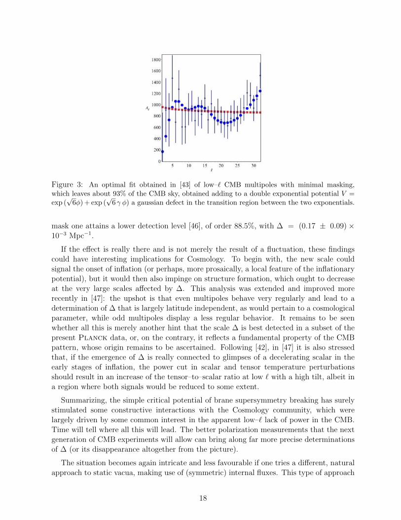
Figure 3: An optimal fit obtained in [43] of low–` CMB multipoles with minimal masking,which leaves about 93% of the CMB sky, obtained adding to a double exponential potential V =exp (

√6φ) + exp (

√6 γ φ) a gaussian defect in the transition region between the two exponentials.

mask one attains a lower detection level [46], of order 88.5%, with ∆ = (0.17 ± 0.09)×10−3 Mpc−1.

If the effect is really there and is not merely the result of a fluctuation, these findingscould have interesting implications for Cosmology. To begin with, the new scale couldsignal the onset of inflation (or perhaps, more prosaically, a local feature of the inflationarypotential), but it would then also impinge on structure formation, which ought to decreaseat the very large scales affected by ∆. This analysis was extended and improved morerecently in [47]: the upshot is that even multipoles behave very regularly and lead to adetermination of ∆ that is largely latitude independent, as would pertain to a cosmologicalparameter, while odd multipoles display a less regular behavior. It remains to be seenwhether all this is merely another hint that the scale ∆ is best detected in a subset of thepresent Planck data, or, on the contrary, it reflects a fundamental property of the CMBpattern, whose origin remains to be ascertained. Following [42], in [47] it is also stressedthat, if the emergence of ∆ is really connected to glimpses of a decelerating scalar in theearly stages of inflation, the power cut in scalar and tensor temperature perturbationsshould result in an increase of the tensor–to–scalar ratio at low ` with a high tilt, albeit ina region where both signals would be reduced to some extent.

Summarizing, the simple critical potential of brane supersymmetry breaking has surelystimulated some constructive interactions with the Cosmology community, which werelargely driven by some common interest in the apparent low–` lack of power in the CMB.Time will tell where all this will lead. The better polarization measurements that the nextgeneration of CMB experiments will allow can bring along far more precise determinationsof ∆ (or its disappearance altogether from the picture).

The situation becomes again intricate and less favourable if one tries a different, naturalapproach to static vacua, making use of (symmetric) internal fluxes. This type of approach

18

Figure 4: An optimal fit of low–` CMB multipoles [45] to the universal cut of [42], with a widerGalactic mask that leaves about 39% of the CMB sky, where oscillations fade out to a large extent.

Figure 5: Posteriors for the parameter ∆ in eq. (3.4) with different maskings around the Galacticplane. The color coding is as follows: solid blue for the 94% mask, thick red for a +30◦ extension,dotted blue for the intermediate masks with +6◦, +12◦, +18◦ and +24◦, dotted red for 36◦.

has accompanied from the beginning, in different forms, the study of supersymmetric vacuain String Theory [48], and it was natural to explore it in this context as well [49]. Oncemore, up to some minor differences one can do this, in an identical fashion, for the USp(32)and U(32) orientifold models, and also for the SO(16)× SO(16) heterotic model reviewedin Section 2. Our starting point was provided by the class of metrics

ds 2 = e2A(r) g(Lk) + dr2 + e2C(r) g(Ek′) , (3.6)

where Lk (Ek′) is a maximally symmetric Lorentzian (Euclidean) spacetime with curvaturek (k′), and by volume form fluxes of the type

Hp+2 = h e (p+1)A(r) + 2β(p)E φ− (8−p)C ε(p+ 1) dr (3.7)

that invade the resulting spacetimes. The key requirement in [49] was the need to avoidlarge string couplings, in contrast with the solution of eq. (3.1), which could be attained inprinciple requiring that the dilaton be stabilized. In this fashion we were led to vacua of the

19

AdS × S type. Most interesting among these are vacua characterized by large sizes, whichare expected to suppress string α′ corrections, with also small values for the string couplinggs = exp(φ), which are expected to suppress string loop corrections. All in all, in a weakly–coupled corner of this type, the low–energy effective field theory would appear a reliabletool to gather some information on String Theory altogether. In [49] we also allowed foran internal gauge field profile, but this was problematic [50] and did not add to potentiallyinteresting options, so that here we shall confine our attention to vacua where only a formprofile is present. Assuming also a constant dilaton profile, the vacuum equations reduceto

T e γE φ = − β(p)E h2

γEe− 2 (8− p)C + 2β

(p)E φ ,

16 k′ e− 2C =

h2

(p + 1 − 2β

(p)E

γE

)e− 2 (8− p)C + 2β

(p)E φ

(7 − p),

(A′)2 = k e− 2A +h2

16(p + 1)

(7 − p +

2 β(p)E

γE

)e− 2 (8− p)C + 2β

(p)E φ . (3.8)

The first is the dilaton equation, which requires for consistency βE < 0, a condition thattranslates into the presence of a three–form flux in the orientifold vacua and of a seven–form flux in the heterotic SO(16)×SO(16) case. This fact determines the available options:AdS3 × S7 in the orientifold case and AdS7 × S3 in the heterotic case. On the other hand,the choice of one or another of the possible values of k, 0 or ±1 selects different slicing ofthe same AdS spacetime. The case k = 0, in particular, captures AdS in Poincare – likecoordinates, and the detailed solutions read

gs ≡ eφ =12

(2hT 3)14

, R4 g3s =

144

T 2, (A′)

2= k e− 2A +

6

R2(3.9)

for the orientifold case (p = 1) and

gs ≡ eφ =

(5

h2 Λ2

) 14

, R4 g5s =

1

Λ2, (A′)

2= k e− 2A +

1

12R2(3.10)

for the heterotic (p = 5) case, where the one–loop contribution Λ, rather than T , accom-panies the potential of eq. (3.3). Both choices allow regions of large h–fluxes, where gs issmall while the scale R determining the radii of the internal sphere and of the AdS space-time is large. All in all, these solutions would thus appear a reliable starting point, butproblems lurk around the corner and for one matter we recently ran across [51], where theauthors had reported on a violation of the Breitenlohner–Freedman bound [52] for one ofthese cases, the AdS3×S7 solution of eq. (3.9), which would also resonate with some recentliterature [53]. These and other related issues are currently under investigation [50].

20

4 Constrained superfields and a four–dimensional toy model

The last issue that we would like to address briefly is the emergence of interesting spring–offs of these and other investigations of broken supersymmetry. The subject proper targetsnon–linear realizations, albeit in the simpler context of four–dimensional models, and hasa life of its own that started long ago, but nonetheless it connects to the preceding sectionsin an interesting fashion.

The one step forward that opened up a host of new possibilities was the recovery of theVolkov–Akulov model [54], which realizes the N = 1 → N = 0 breaking in a non–linearregime, via a chiral superfield Φ subject to the quadratic constraint [55–57]

Φ2 = 0 . (4.1)

This constraint replaces the complex scalar by a fermion bilinear, so that

Φ =ψ ψ

2F+√

2 θα ψα + θ2 F . (4.2)

The Volkov–Akulov model then emerges from the Wess–Zumino Lagrangian with a Polonyiterm, in the presence of the constraint (4.1), up to a complicated field redefinition that wasspelled out in [58].

Constrained superfields can also provide very instructive playgrounds in applicationsof supergravity to Cosmology, since for one matter they reduce to a minimum the fieldsinvolved in model building. This endeavour started with the example of the Starobin-sky model [59], whose realization [60] obtains coupling supergravity to an ordinary Wess–Zumino multiplet and a constrained one. Many interesting models then followed this workand [61], which also include different realizations of the minimal coupling of supergravity tothe Volkov–Akulov model [62]. These developments are reviewed in [63], and the upshot isthat, in all cases, one can apply the standard formula for the supergravity potential of [64],

V = eG[(G−1

)ij Gi Gj − 3]

with G = K + log |W|2 , (4.3)

while enforcing the constraint (4.1) only at the end.

A second major step along this line was attained in the 1990’s. It is the recovery of thesupersymmetric Born–Infeld model, which realizes the N = 2 → N = 1 breaking [65], viaa quadratic constraint linking to one another a chiral and a vector multiplet according to

C2 : WαWα − 2 Φ

(1

4D

2Φ − m

)= 0 . (4.4)

The crucial difference between this case and the preceding one is that now, starting fromN = 2, one ends up with N = 1 supersymmetry. There was some discussion as to whetherthis would be possible at all, and this development owes to the original considerationsin [66] and to the explicit linear models of [67] and [68]. In retrospect, the end result can be

21

regarded as a toy model for a standard D brane, whose insertion in the vacuum halves itsoriginal amount of supersymmetry. The supersymmetric Born–Infeld theory, with a scaledetermined by the real “magnetic” charge m, then emerges from the Polonyi term, sincethe constraint eliminates all kinetic terms in

L = Re

[1

2

∫d2θWαWα + (m − i ec)

∫d2θΦ

]+

∫d4θ Φ Φ . (4.5)

These results also afford a natural generalization to the case of a number of Abelianmultiplets, whereby the constraint of eq. (4.4) becomes [69]

dABC

[WαBWC

α − 2 ΦB

(1

4D

2ΦC − mC

)]= 0 , (4.6)

which might provide some useful information on the long–sought non–Abelian Born–Infeldtheory associated to D-brane stacks [70]. It would be interesting to characterize its micro-scopic origin and its role in String Theory.

Let us conclude with a more recent result, described in [71], which concerns the non–linear N = 2 → N = 0 breaking in a vector multiplet, and is therefore a simple four–dimensional toy model of brane supersymmetry breaking. The relevant constraint is nowcubic, and reads

ΦWαWα − Φ2

(1

4D

2Φ − m

)= 0 −→ Φ3 = 0 , Φ2Wα = 0 . (4.7)

One can show that, aside from a singular corner where the N = 2 → N = 1 breaking isrecovered, this cubic constraint eliminates the complex scalar of the Wess-Zumino multiplet,leaving the gauge field and the two fermions of the original multiplets, which are the twogoldstini of the system. Notice that, in contrast with the N = 1→ N = 0 case of [65], herea Born–Infeld structure of the remaining low–energy interactions is not implied. Otherrecent works dealing with the N = 2 → N = 0 case, also from the vantage point ofVolkov–Akulov model, can be found in [72].

We have addressed these developments from the vantage point of brane supersymmetrybreaking, but the four–dimensional counterpart of the tadpole potentials in eq. (2.23) and(2.24) is also the uplift potential of the KKLT construction [73]. The work of [74], wherecombinations of different constrained N = 1 multiplets are used to characterize the four–dimensional content of the associated branes, is also close in spirit to this simple example.

Acknowledgements

J.M. is grateful to Scuola Normale and A.S. is grateful to CPhT–Ecole Polytechnique,APC–U. Paris VII and CERN-TH for the kind hospitality while the work reviewed herewas in progress. A.S. was supported in part by Scuola Normale Superiore and by INFN(IS CSN4-GSS-PI). We are also grateful to C. Angelantonj, I. Basile, E. Dudas, S. Fer-rara, A. Gruppuso, N. Kitazawa, M. Lattanzi, N. Mandolesi, P. Natoli and G. Pradisifor extensive discussions and/or collaborations on related issues and/or comments on themanuscript.

22

References

[1] For reviews see: M. B. Green, J. H. Schwarz and E. Witten, “Superstring Theory”, 2vols., Cambridge, UK: Cambridge Univ. Press (1987); J. Polchinski, “String theory”,2 vols. Cambridge, UK: Cambridge Univ. Press (1998); C. V. Johnson, “D-branes,”USA: Cambridge Univ. Press (2003) 548 p; B. Zwiebach, “A first course in stringtheory” Cambridge, UK: Cambridge Univ. Press (2004); K. Becker, M. Becker andJ. H. Schwarz, “String theory and M-theory: A modern introduction” Cambridge, UK:Cambridge Univ. Press (2007); E. Kiritsis, “String theory in a nutshell”, Princeton,NJ: Princeton Univ. Press (2007); P. West, “Introduction to strings and branes,”Cambridge: Cambridge Univ. Press (2012).

[2] D. Z. Freedman, P. van Nieuwenhuizen and S. Ferrara, Phys. Rev. D 13 (1976)3214; S. Deser and B. Zumino, Phys. Lett. 62B (1976) 335. For detailed reviews see:D. Z. Freedman and A. Van Proeyen, “Supergravity,” Cambridge, UK: CambridgeUniv. Pr. (2012). For an early review see: P. Van Nieuwenhuizen, Phys. Rept. 68(1981) 189. For an elementaty overview of some of the main developments see: S. Fer-rara and A. Sagnotti, “Supergravity at 40: Reflections and Perspectives,” Riv. NuovoCim. 40 (2017) no.6, 1 [J. Phys. Conf. Ser. 873 (2017) no.1, 012014] [arXiv:1702.00743[hep-th]].

[3] D. J. Gross, J. A. Harvey, E. J. Martinec and R. Rohm, Phys. Rev. Lett. 54 (1985)502, Nucl. Phys. B 256 (1985) 253, Nucl. Phys. B 267 (1986) 75.

[4] M. B. Green and J. H. Schwarz, Phys. Lett. 149B (1984) 117.

[5] A. Sagnotti, in Cargese ’87, “Non-Perturbative Quantum Field Theory”, eds. G. Macket al (Pergamon Press, 1988), p. 521, arXiv:hep-th/0208020; G. Pradisi and A. Sag-notti, Phys. Lett. B 216 (1989) 59; P. Horava, Nucl. Phys. B 327 (1989) 461, Phys.Lett. B 231 (1989) 251; M. Bianchi and A. Sagnotti, Phys. Lett. B 247 (1990) 517,Nucl. Phys. B 361 (1991) 519; M. Bianchi, G. Pradisi and A. Sagnotti, Nucl. Phys. B376 (1992) 365; A. Sagnotti, Phys. Lett. B 294 (1992) 196 [arXiv:hep-th/9210127].For reviews see: E. Dudas, Class. Quant. Grav. 17 (2000) R41 [arXiv:hep-ph/0006190];C. Angelantonj and A. Sagnotti, Phys. Rept. 371 (2002) 1 [Erratum-ibid. 376 (2003)339] [arXiv:hep-th/0204089].

[6] L. Alvarez-Gaume, P. H. Ginsparg, G. W. Moore and C. Vafa, Phys. Lett. B 171(1986) 155; L. J. Dixon and J. A. Harvey, Nucl. Phys. B 274 (1986) 93.

[7] L. J. Dixon, J. A. Harvey, C. Vafa and E. Witten, Nucl. Phys. B 261 (1985) 678; Nucl.Phys. B 274 (1986) 285.

[8] A. Sagnotti, In *Palaiseau 1995, Susy 95* 473-484 [hep-th/9509080], Nucl. Phys. Proc.Suppl. 56B (1997) 332 [hep-th/9702093].

[9] N. Seiberg and E. Witten, Nucl. Phys. B 276 (1986) 272.

23

[10] S. Sugimoto, Prog. Theor. Phys. 102 (1999) 685 [arXiv:hep-th/9905159];

[11] I. Antoniadis, E. Dudas and A. Sagnotti, Phys. Lett. B 464 (1999) 38 [arXiv:hep-th/9908023]; C. Angelantonj, Nucl. Phys. B 566 (2000) 126 [arXiv:hep-th/9908064];G. Aldazabal and A. M. Uranga, JHEP 9910 (1999) 024 [arXiv:hep-th/9908072];C. Angelantonj, I. Antoniadis, G. D’Appollonio, E. Dudas and A. Sagnotti, Nucl.Phys. B 572 (2000) 36 [arXiv:hep-th/9911081]; E. Dudas and J. Mourad, Phys. Lett.B 514 (2001) 173 [hep-th/0012071]; G. Pradisi and F. Riccioni, Nucl. Phys. B 615(2001) 33 [hep-th/0107090].

[12] J. Polchinski, Phys. Rev. Lett. 75 (1995) 4724 [hep-th/9510017].

[13] P. K. Townsend, Phys. Lett. B 350 (1995) 184 [hep-th/9501068]; E. Witten, Nucl.Phys. B 443 (1995) 85 [hep-th/9503124].

[14] A. Neveu and J. H. Schwarz, Nucl. Phys. B 31 (1971) 86; P. Ramond, Phys. Rev. D 3(1971) 2415.

[15] F. Gliozzi, J. Scherk and D. I. Olive, Nucl. Phys. B 122 (1977) 253.

[16] For a review of their properties see, for instance: E. T. Whittaker and G. N. Watson,“A course in Modern Analysis”, Cambridge: Cambridge Univ. Press (1920).

[17] S. Kachru, J. Kumar and E. Silverstein, Phys. Rev. D 59 (1999) 106004 [hep-th/9807076]; J. A. Harvey, Phys. Rev. D 59 (1999) 026002 [hep-th/9807213]; C. Ange-lantonj, I. Antoniadis and K. Forger, Nucl. Phys. B 555 (1999) 116 [hep-th/9904092].

[18] S. Abel, K. R. Dienes and E. Mavroudi, Phys. Rev. D 91 (2015) no.12, 126014[arXiv:1502.03087 [hep-th]]; C. Kounnas and H. Partouche, PoS PLANCK 2015 (2015)070 [arXiv:1511.02709 [hep-th]], Nucl. Phys. B 913 (2016) 593 [arXiv:1607.01767 [hep-th]]; I. Florakis and J. Rizos, Nucl. Phys. B 913 (2016) 495 [arXiv:1608.04582 [hep-th]].

[19] W. Fischler and L. Susskind, Phys. Lett. B 171 (1986) 383, Phys. Lett. B 173 (1986)262, E. Dudas, M. Nicolosi, G. Pradisi and A. Sagnotti, Nucl. Phys. B 708 (2005) 3,[arXiv:hep-th/0410101]; N. Kitazawa, Phys. Lett. B 660 (2008) 415 [arXiv:0801.1702[hep-th]], R. Pius, A. Rudra and A. Sen, JHEP 1410 (2014) 70, [arXiv:1404.6254[hep-th]].

[20] J. E. Paton and H. M. Chan, Nucl. Phys. B 10 (1969) 516; J. H. Schwarz, Phys. Rept.89 (1982) 223; N. Marcus and A. Sagnotti, Phys. Lett. 119B (1982) 97, Phys. Lett.B 188 (1987) 58.

[21] E. Witten, JHEP 9802 (1998) 006 [hep-th/9712028].

[22] A. Sagnotti, hep-th/9302099.

24

[23] A. Sen, JHEP 9806 (1998) 007 [hep-th/9803194], JHEP 9808 (1998) 010 [hep-th/9805019]; O. Bergman and M. R. Gaberdiel, Phys. Lett. B 441 (1998) 133 [hep-th/9806155]. For reviews see: A. Sen, hep-th/9904207; A. Lerda and R. Russo, Int. J.Mod. Phys. A 15 (2000) 771 [hep-th/9905006].

[24] E. Dudas and J. Mourad, Nucl. Phys. B 598 (2001) 189 [hep-th/0010179]; E. Dudas,J. Mourad and A. Sagnotti, Nucl. Phys. B 620 (2002) 109 [hep-th/0107081].

[25] A. Armoni and B. Kol, JHEP 9907 (1999) 011 [hep-th/9906081]; C. Angelantonj andA. Armoni, Nucl. Phys. B 578 (2000) 239 [hep-th/9912257]; A. Armoni, M. Shifmanand G. Veneziano, Nucl. Phys. B 667 (2003) 170 [hep-th/0302163], Phys. Rev. Lett.91 (2003) 191601 [hep-th/0307097], In *Shifman, M. (ed.) et al.: From fields to strings,vol. 1* 353-444 [hep-th/0403071]; A. Armoni and V. Niarchos, arXiv:1711.04832 [hep-th].

[26] G. Pradisi, A. Sagnotti and Y. S. Stanev, Phys. Lett. B 354 (1995) 279 [hep-th/9503207], Phys. Lett. B 356 (1995) 230 [hep-th/9506014], Phys. Lett. B 381 (1996)97 [hep-th/9603097].

[27] D. Fioravanti, G. Pradisi and A. Sagnotti, Phys. Lett. B 321 (1994) 349 [hep-th/9311183].

[28] D. C. Lewellen, Nucl. Phys. B 372 (1992) 654.

[29] L. R. Huiszoon, A. N. Schellekens and N. Sousa, Phys. Lett. B 470 (1999) 95 [hep-th/9909114]; J. Fuchs, L. R. Huiszoon, A. N. Schellekens, C. Schweigert and J. Walcher,Phys. Lett. B 495 (2000) 427 [hep-th/0007174].

[30] D. Gepner and E. Witten, Nucl. Phys. B 278 (1986) 493.

[31] E. P. Verlinde, Nucl. Phys. B 300 (1988) 360.

[32] See, for instance, N. Kitazawa, Mod. Phys. Lett. A 32 (2017) no.29, 1750150[arXiv:1706.07161 [hep-th]], and references therein.

[33] E. Dudas and J. Mourad, Phys. Lett. B 486 (2000) 172 [hep-th/0004165].

[34] J. J. Halliwell, Phys. Lett. B 185 (1987) 341; L. F. Abbott and M. B. Wise, Nucl.Phys. B 244 (1984) 541; D. H. Lyth and E. D. Stewart, Phys. Lett. B 274 (1992)168; I. P. C. Heard and D. Wands, Class. Quant. Grav. 19 (2002) 5435 [arXiv:gr-qc/0206085]; N. Ohta, Phys. Rev. Lett. 91 (2003) 061303 [arXiv:hep-th/0303238];S. Roy, Phys. Lett. B 567 (2003) 322 [arXiv:hep-th/0304084]; P. K. Townsend andM. N. R. Wohlfarth, Phys. Rev. Lett. 91 (2003) 061302 [arXiv:hep-th/0303097]; Class.Quant. Grav. 21 (2004) 5375 [arXiv:hep-th/0404241]; R. Emparan and J. Garriga,JHEP 0305 (2003) 028 [arXiv:hep-th/0304124]; E. Bergshoeff, A. Collinucci, U. Gran,M. Nielsen and D. Roest, Class. Quant. Grav. 21 (2004) 1947 [hep-th/0312102];A. A. Andrianov, F. Cannata and A. Y. Kamenshchik, JCAP 1110 (2011) 004[arXiv:1105.4515 [gr-qc]].

25

[35] J. G. Russo, Phys. Lett. B 600 (2004) 185 [arXiv:hep-th/0403010];

[36] P. Fre, A. Sagnotti and A. S. Sorin, Nucl. Phys. B 877 (2013) 1028 [arXiv:1307.1910[hep-th]].

[37] E. Dudas, N. Kitazawa and A. Sagnotti, Phys. Lett. B 694 (2010) 80 [arXiv:1009.0874[hep-th]];

[38] C. Condeescu and E. Dudas, JCAP 1308 (2013) 013 [arXiv:1306.0911 [hep-th]].

[39] A. A. Starobinsky, Phys. Lett. B 91 (1980) 99; D. Kazanas, Astrophys. J. 241 (1980)L59; K. Sato, Phys. Lett. B 99 (1981) 66; A. H. Guth, Phys. Rev. D 23 (1981)347; A. D. Linde, Phys. Lett. B 108 (1982) 389; A. Albrecht and P. J. Steinhardt,Phys. Rev. Lett. 48 (1982) 1220; A. D. Linde, Phys. Lett. B 129 (1983) 177; Forreviews see: N. Bartolo, E. Komatsu, S. Matarrese and A. Riotto, Phys. Rept. 402(2004) 103 [astro-ph/0406398]; V. Mukhanov, “Physical foundations of cosmology,”Cambridge, UK: Univ. Pr. (2005); S. Weinberg, “Cosmology,” Oxford, UK: OxfordUniv. Pr. (2008); D. H. Lyth and A. R. Liddle, “The primordial density perturbation:Cosmology, inflation and the origin of structure,” Cambridge, UK: Cambridge Univ.Pr. (2009); D. S. Gorbunov and V. A. Rubakov, “Introduction to the theory of theearly universe: Cosmological perturbations and inflationary theory,” Hackensack, USA:World Scientific (2011); J. Martin, C. Ringeval and V. Vennin, Phys. Dark Univ. 5-6(2014) 75 [arXiv:1303.3787 [astro-ph.CO]].

[40] D. N. Spergel et al. [WMAP Collaboration], Astrophys. J. Suppl. 148, 175 (2003)[astro-ph/0302209].

[41] P. A. R. Ade et al. [Planck Collaboration], Astron. Astrophys. 594 (2016)A13 [arXiv:1502.01589 [astro-ph.CO]], Astron. Astrophys. 594 (2016) A16[arXiv:1506.07135 [astro-ph.CO]]; N. Aghanim et al. [Planck Collaboration], Astron.Astrophys. 594 (2016) A11 [arXiv:1507.02704 [astro-ph.CO]].

[42] E. Dudas, N. Kitazawa, S. P. Patil and A. Sagnotti, JCAP 1205 (2012) 012[arXiv:1202.6630 [hep-th]]; A. Sagnotti, Phys. Part. Nucl. Lett. 11 (2014) 836[arXiv:1303.6685 [hep-th]].

[43] N. Kitazawa and A. Sagnotti, JCAP 1404 (2014) 017 [arXiv:1402.1418 [hep-th]], EPJWeb Conf. 95 (2015) 03031 [arXiv:1411.6396 [hep-th]], Mod. Phys. Lett. A 30 (2015)no.28, 1550137 [arXiv:1503.04483 [hep-th]].

[44] V. F. Mukhanov and G. V. Chibisov, JETP Lett. 33 (1981) 532 [Pisma Zh. Eksp.Teor. Fiz. 33 (1981) 549].

[45] A. Sagnotti, Mod. Phys. Lett. A 32 (2016) no.01, 1730001 [Subnucl. Ser. 53 (2017)289] [arXiv:1509.08204 [astro-ph.CO]].

26

[46] A. Gruppuso and A. Sagnotti, Int. J. Mod. Phys. D 24 (2015) no.12, 1544008[arXiv:1506.08093 [astro-ph.CO]]; A. Gruppuso, N. Kitazawa, N. Mandolesi, P. Na-toli and A. Sagnotti, Phys. Dark Univ. 11 (2016) 68 [arXiv:1508.00411 [astro-ph.CO]].

[47] A. Gruppuso, N. Kitazawa, M. Lattanzi, N. Mandolesi, P. Natoli and A. Sagnotti, toappear.

[48] P. Candelas, G. T. Horowitz, A. Strominger and E. Witten, Nucl. Phys. B 258 (1985)46.

[49] J. Mourad and A. Sagnotti, Phys. Lett. B 768 (2017) 92 [arXiv:1612.08566 [hep-th]].

[50] I. Basile, J. Mourad and A.S, work in progress.

[51] S. S. Gubser and I. Mitra, JHEP 0207 (2002) 044 [hep-th/0108239].

[52] P. Breitenlohner and D. Z. Freedman, Annals Phys. 144 (1982) 249.

[53] N. Arkani-Hamed, L. Motl, A. Nicolis and C. Vafa, JHEP 0706 (2007) 060 [hep-th/0601001]. See also: D. Lust and E. Palti, arXiv:1709.01790 [hep-th], and referencestherein.

[54] D. V. Volkov and V. P. Akulov, Phys. Lett. 46B (1973) 109.

[55] M. Rocek, Phys. Rev. Lett. 41 (1978) 451; E. A. Ivanov and A. A. Kapustnikov, J.Phys. A 11 (1978) 2375; U. Lindstrom and M. Rocek, Phys. Rev. D 19 (1979) 2300.

[56] R. Casalbuoni, S. De Curtis, D. Dominici, F. Feruglio and R. Gatto, Phys. Lett. B220 (1989) 569; A. Brignole, F. Feruglio and F. Zwirner, JHEP 9711 (1997) 001[hep-th/9709111].

[57] Z. Komargodski and N. Seiberg, JHEP 0909 (2009) 066 [arXiv:0907.2441 [hep-th]];

[58] S. M. Kuzenko and S. J. Tyler, Phys. Lett. B 698 (2011) 319 [arXiv:1009.3298 [hep-th]].

[59] A. A. Starobinsky, Phys. Lett. 91B (1980) 99.

[60] I. Antoniadis, E. Dudas, S. Ferrara and A. Sagnotti, Phys. Lett. B 733 (2014) 32[arXiv:1403.3269 [hep-th]].

[61] S. Ferrara, R. Kallosh and A. Linde, JHEP 1410 (2014) 143doi:10.1007/JHEP10(2014)143 [arXiv:1408.4096 [hep-th]]; R. Kallosh and A. Linde,JCAP 1501 (2015) 025 [arXiv:1408.5950 [hep-th]]; G. Dall’Agata and F. Zwirner,JHEP 1412 (2014) 172 [arXiv:1411.2605 [hep-th]].

[62] L. Alvarez-Gaume, A. Kehagias, C. Kounnas, D. Lust and A. Riotto, Fortsch. Phys. 64(2016) no.2-3, 176 [arXiv:1505.07657 [hep-th]]; S. Ferrara, A. Kehagias and M. Porrati,JHEP 1508 (2015) 001 [arXiv:1506.01566 [hep-th]]; E. Dudas, S. Ferrara, A. Kehagiasand A. Sagnotti, JHEP 1509 (2015) 217 [arXiv:1507.07842 [hep-th]]; F. Hasegawa

27

and Y. Yamada, JHEP 1510 (2015) 106 [arXiv:1507.08619 [hep-th]]; E. A. Bergshoeff,D. Z. Freedman, R. Kallosh and A. Van Proeyen, Phys. Rev. D 92 (2015) no.8, 085040Erratum: [Phys. Rev. D 93 (2016) no.6, 069901] [arXiv:1507.08264 [hep-th]]; S. Fer-rara, M. Porrati and A. Sagnotti, Phys. Lett. B 749 (2015) 589 [arXiv:1508.02939[hep-th]]; I. Antoniadis and C. Markou, Eur. Phys. J. C 75 (2015) no.12, 582[arXiv:1508.06767 [hep-th]]; N. Cribiori, G. Dall’Agata, F. Farakos and M. Porrati,Phys. Lett. B 764 (2017) 228 [arXiv:1611.01490 [hep-th]].

[63] A. Sagnotti and S. Ferrara, PoS PLANCK 2015 (2015) 113 [arXiv:1509.01500 [hep-th]]; S. Ferrara, A. Kehagias and A. Sagnotti, Int. J. Mod. Phys. A 31 (2016) no.25,1630044 [arXiv:1605.04791 [hep-th]].

[64] E. Cremmer, S. Ferrara, L. Girardello and A. Van Proeyen, Nucl. Phys. B 212 (1983)413.

[65] J. Bagger and A. Galperin, Phys. Rev. D 55 (1997) 1091 [hep-th/9608177].

[66] J. Hughes and J. Polchinski, Nucl. Phys. B 278 (1986) 147; J. Hughes, J. Liu andJ. Polchinski, Phys. Lett. B 180 (1986) 370.

[67] I. Antoniadis, H. Partouche and T. R. Taylor, Phys. Lett. B 372 (1996) 83 [hep-th/9512006].

[68] S. Cecotti, L. Girardello and M. Porrati, Phys. Lett. 168B (1986) 83; S. Ferrara,L. Girardello and M. Porrati, Phys. Lett. B 366 (1996) 155, [hep-th/9510074], Phys.Lett. B 376 (1996) 275 [hep-th/9512180].

[69] S. Ferrara, M. Porrati and A. Sagnotti, JHEP 1412 (2014) 065 [arXiv:1411.4954 [hep-th]]; S. Ferrara, M. Porrati, A. Sagnotti, R. Stora and A. Yeranyan, Fortsch. Phys. 63(2015) 189 [arXiv:1412.3337 [hep-th]].

[70] Fora review see: A. A. Tseytlin, In *Shifman, M.A. (ed.): The many faces of thesuperworld* 417-452 [hep-th/9908105].

[71] E. Dudas, S. Ferrara and A. Sagnotti, JHEP 1708 (2017) 109 [arXiv:1707.03414 [hep-th]].

[72] N. Cribiori, G. Dall’Agata and F. Farakos, Phys. Rev. D 94 (2016) no.6,065019 [arXiv:1607.01277 [hep-th]]; S. M. Kuzenko and G. Tartaglino-Mazzucchelli,arXiv:1707.07390 [hep-th].

[73] S. Kachru, R. Kallosh, A. D. Linde and S. P. Trivedi, Phys. Rev. D 68 (2003) 046005[hep-th/0301240].

[74] R. Kallosh, B. Vercnocke and T. Wrase, JHEP 1609 (2016) 063 [arXiv:1606.09245[hep-th]].

28