an uncertainty principle for star formation – ii. a new ... · an uncertainty principle for star...
TRANSCRIPT

MNRAS 000, 1–83 (2018) Preprint 5 September 2018 Compiled using MNRAS LATEX style file v3.0
An uncertainty principle for star formation – II. A new method forcharacterising the cloud-scale physics of star formation andfeedback across cosmic history
J. M. Diederik Kruijssen,1,2,3? Andreas Schruba,4 Alexander P. S. Hygate,2,1
Chia-Yu Hu,3,5 Daniel T. Haydon1 and Steven N. Longmore61Astronomisches Rechen-Institut, Zentrum fur Astronomie der Universitat Heidelberg, Monchhofstraße 12-14, 69120 Heidelberg, Germany2Max-Planck Institut fur Astronomie, Konigstuhl 17, 69117 Heidelberg, Germany3Max-Planck Institut fur Astrophysik, Karl-Schwarzschild-Straße 1, 85748 Garching, Germany4Max-Planck Institut fur Extraterrestrische Physik, Giessenbachstraße 1, 85748 Garching, Germany5Center for Computational Astrophysics, 160 Fifth Avenue, New York, NY 10010, USA6Astrophysics Research Institute, Liverpool John Moores University, IC2, Liverpool Science Park, 146 Brownlow Hill, Liverpool L3 5RF, United Kingdom
Accepted 2018 April 27. Received 2018 April 23; in original form 2017 October 5.
ABSTRACTThe cloud-scale physics of star formation and feedback represent the main uncertainty ingalaxy formation studies. Progress is hampered by the limited empirical constraints outsidethe restricted environment of the Local Group. In particular, the poorly-quantified time evolu-tion of the molecular cloud lifecycle, star formation, and feedback obstructs robust predictionson the scales smaller than the disc scale height that are resolved in modern galaxy formationsimulations. We present a new statistical method to derive the evolutionary timeline of molec-ular clouds and star-forming regions. By quantifying the excess or deficit of the gas-to-stellarflux ratio around peaks of gas or star formation tracer emission, we directly measure the rela-tive rarity of these peaks, which allows us to derive their lifetimes. We present a step-by-step,quantitative description of the method and demonstrate its practical application. The method’saccuracy is tested in nearly 300 experiments using simulated galaxy maps, showing that it iscapable of constraining the molecular cloud lifetime and feedback time-scale to < 0.1 dexprecision. Access to the evolutionary timeline provides a variety of additional physical quan-tities, such as the cloud-scale star formation efficiency, the feedback outflow velocity, themass loading factor, and the feedback energy or momentum coupling efficiencies to the am-bient medium. We show that the results are robust for a wide variety of gas and star formationtracers, spatial resolutions, galaxy inclinations, and galaxy sizes. Finally, we demonstrate thatour method can be applied out to high redshift (z . 4) with a feasible time investment oncurrent large-scale observatories. This is a major shift from previous studies that constrainedthe physics of star formation and feedback in the immediate vicinity of the Sun.
Key words: stars: formation – ISM: evolution – galaxies: evolution – galaxies: formation –galaxies: ISM – galaxies: stellar content
1 INTRODUCTION
Current theoretical and numerical models aiming to reproduce theobserved galaxy population are strongly limited by uncertainties inthe baryonic physics (e.g. Hopkins et al. 2011; Haas et al. 2013;Vogelsberger et al. 2014; Schaye et al. 2015). While the bound-ary conditions provided by cosmology and the hierarchical growthof the dark matter haloes in which galaxies reside are relativelywell-constrained (e.g. Springel et al. 2005b; Planck Collaborationet al. 2014), connecting these haloes to the visible galaxy popula-tion hinges critically on the unknown physics of star formation andfeedback (McKee & Ostriker 2007; Kennicutt & Evans 2012).
Galaxy formation simulations generally describe star forma-tion using the phenomenological, galaxy-scale relations betweenthe gas mass and the star formation rate (SFR), observed fromnearby spiral galaxies (e.g. Bigiel et al. 2008; Schruba et al. 2011;Kennicutt & Evans 2012; Leroy et al. 2013) out to high redshift(e.g. Daddi et al. 2010; Genzel et al. 2010; Tacconi et al. 2013).Broadly, these galactic ‘star formation relations’ represent varia-tions of the form
SFR =εsfτsfMgas, (1)
where εsf represents the star formation efficiency, τsf is the starformation time-scale, and Mgas indicates the gas mass. One ofthe main reasons that the physics underpinning the galactic starformation relation have been so challenging to constrain (see e.g.
c© 2018 The Authors
arX
iv:1
805.
0001
2v2
[as
tro-
ph.G
A]
4 S
ep 2
018

2 J. M. D. Kruijssen et al.
Krumholz & McKee 2005; Hennebelle & Chabrier 2011; Ostriker& Shetty 2011; Padoan & Nordlund 2011; Krumholz et al. 2012,among many others) is that the star formation efficiency and time-scale represent degenerate quantities in the above expression. Itis impossible to determine from the star formation relation alonewhether star formation is rapid and inefficient or slow and effi-cient. This problem is exacerbated by the fact that both quantitiesare notoriously hard to measure – star formation takes place ontime-scales much longer than a human lifetime, implying that τsfcannot be measured directly and εsf cannot be obtained by simplyconsidering the initial and final states of a single system. However,knowing either εsf or τsf would allow one to immediately constrainthe other. Analogously to equation (1), the commonly-used star for-mation ‘recipes’ in galaxy formation simulations generally assumethat gas is turned into stars on some time-scale τsf with some effi-ciency εsf . Both quantities are unknown on the small (10–100 pc)scales of the individual gas clouds resolved in modern galaxy for-mation simulations, but strongly affect the structure of simulatedgalaxies (e.g. Hopkins et al. 2013; Braun & Schmidt 2015; Se-menov et al. 2016). It is therefore a priority to obtain empiricalconstraints on these quantities and their variation with the galacticenvironment.
Likewise, the deposition of mass, momentum and energy byfeedback is often based on a simple representation of supernova(SN) feedback, i.e. by injecting an amount of energy appropri-ate for the expected number of SNe into the interstellar medium(ISM) surrounding each young stellar population (e.g. Springel &Hernquist 2003) or by defining an empirical mass outflow rate inunits of the SFR that may depend on the local galactic environmen-tal conditions (e.g. Oppenheimer & Dave 2006, 2008). However,it is shown by theory (e.g. Murray et al. 2010; Dale et al. 2013;Agertz et al. 2013) and observations (e.g. Pellegrini et al. 2010;Lopez et al. 2011, 2014) of nearby star-forming regions that otherfeedback mechanisms (e.g. photoionization, stellar winds, radiationpressure) can be at least equally effective as SNe (see e.g. the recentreviews by Kruijssen 2013; Krumholz et al. 2014; Dale 2015). Ob-taining an empirically-motivated prescription for stellar feedbackin galaxy formation simulations is crucial, because most discrep-ancies between the observed and simulated galaxy populations canbe alleviated with a suitable (but possibly ad-hoc) choice of feed-back model (e.g. Hopkins et al. 2014; Schaye et al. 2015).
In Kruijssen & Longmore (2014, hereafter KL14), we pre-sented a new statistical model, named the ‘uncertainty principle forstar formation’, which explains how the galaxy-scale star formationproperties of a galaxy emerge by the summation over its constituentpopulation of independent star-forming regions. In particular, the‘KL14 principle’ predicts that the star formation relation changesform towards small (. kpc) spatial scales in a way that dependssensitively on the evolutionary timeline of star-forming regions.We showed that it can therefore be used to directly measure theefficiencies and time-, size- and velocity-scales of cloud collapse,star formation, and feedback without requiring individual clouds tobe resolved. By comparing the flux ratios between tracers of gasand star formation on 0.1–1 kpc scales across a galaxy, the methodeffectively counts the relative occurrence of these phases withoutresolving them spatially, thereby directly constraining their char-acteristic lifetimes and spatial separations. The method is easy toapply and could potentially be used to characterize cloud-scale starformation and feedback across cosmic history.
The KL14 principle does not provide the first attempt of char-acterising cloud-scale star formation and feedback. For instance,molecular cloud lifetimes have been estimated in the Local Group
for the Milky Way, the Magellanic Clouds, and M33 (Engargiolaet al. 2003; Kawamura et al. 2009; Murray 2011), as well as forM51 (Meidt et al. 2015), stellar feedback energy and momentumdeposition rates have been determined for the Magellanic Clouds(Pellegrini et al. 2010; Lopez et al. 2011, 2014), and the rapid-ity and efficiency of star formation have been quantified for star-forming clouds in the Milky Way, albeit with a broad range of out-comes (e.g. Elmegreen 2000; Krumholz & Tan 2007; Evans et al.2009; Kruijssen et al. 2015; Barnes et al. 2017). The common short-coming of the methods used in these studies is that they can onlybe applied to the limited range of galactic environments present inLocal Group galaxies or to exceptionally high-resolution observa-tions of external galaxies, because they require individual clouds tobe resolved. The main improvement of the KL14 principle is that itcan be applied out to much larger distances because only the typicalseparation length between clouds must be (marginally) resolved. Inaddition, the robust statistical basis of the method enables its appli-cation to large galaxy samples with little computational effort orhuman intervention.
In this paper, a general framework for applying the KL14 prin-ciple is presented and the method is validated using numerical sim-ulations of isolated disc galaxies. We first summarise the basic con-cepts behind the KL14 principle (Section 2). We then present astep-by-step description of the method’s application to integratedintensity maps of gas and star formation tracers across galaxies(Section 3). We validate the process by applying it to numericalsimulations of disc galaxies and verifying the accuracy of the ex-tracted quantities (Section 4), the results of which are summarisedas a set of guidelines for the reliable application of the method(Section 4.4). The extracted quantities are then used to calculateseveral derived quantities that are demonstrated to accurately de-scribe cloud-scale star formation and feedback (Section 5). We thenuse the several performed tests of the method to determine out towhich distances reliable constraints on cloud-scale star formationand feedback can be obtained (Section 6). We include an exten-sive discussion of the method’s caveats and limitations, as well asof its planned future improvements (Section 7). The paper is fin-ished with a summary of our conclusions and a discussion of themethod’s potential for future applications (Section 8). Finally, Ap-pendices A–D provide the necessary background for a number oftechnical considerations in this paper, as well as the complete setof test results used in Section 4.
The reader less interested in the quantitative details of themethod and its validation can refer to parts of the paper for a qual-itative summary. For a cursory overview of the results, we recom-mend consulting only Sections 1, 2, 3.1, 4.4, 6, and 8. This effec-tively shortens the paper to a little over ten pages.
2 SUMMARY OF THE FORMALISM
The fundamental concept underpinning the KL14 principle is thata galaxy consists of some number of independent star-forming re-gions (hereafter ‘independent regions’) separated by some length-scale λ, which each reside in an evolutionary phase independentlyof their neighbours. Figure 1 shows the evolutionary timeline fora single independent region. The physical meaning of the phasesdepends on the adopted tracers. While this example shows the tran-sition from gas to stars, a similar timeline can be constructed forpairs of gas tracers or star formation tracers. By combining manysuch tracer pairs, a long timeline of several different, partially-overlapping phases is obtained.
MNRAS 000, 1–83 (2018)

Cloud-scale star formation across cosmic history 3
Gas StarsOverlap
Time
tgas
tstar
tover
τ
Figure 1. Schematic representation of the timeline of an individual star-forming region, which starts out being visible in gas tracer emission(e.g. HI, CO or HCN), and ends up being visible in young stellar traceremission (e.g. Hα or FUV). In between, there is an overlap phase duringwhich both tracers are visible. The duration of each corresponding time-scale is indicated below the timeline.
2.1 The star formation relation must break down on smallspatial scales
In its most general form, the first result of KL14 is that if a macro-scopic correlation (e.g. the star formation relation between the gasmass Mgas and the SFR) is caused by a time evolution (e.g. theconversion from gas to stars), then it must break down on smallspatial scales because the subsequent phases of that time evolutionare being resolved. When treating galaxies as a whole, this is gen-erally not a concern, because most often they consist of a numberof independent regions sufficiently large to ensure that the timelineof Figure 1 is well-sampled.1 However, there must be some spa-tial scale below which this is no longer true. Given some typicalseparation length λ between independent regions, the KL14 prin-ciple predicts that the relative uncertainty or Poisson error on thestar formation relation is only smaller than unity (i.e. the relationis well-defined and does not ‘break down’) when the condition issatisfied that
∆x∆t1/2 > λτ1/2. (2)
Here, ∆x is the size scale over which the star formation relationis evaluated (the ‘aperture size’), ∆t is the shortest2 evolutionaryphase from Figure 1, λ is the separation length of independent re-gions, and τ is the total duration of the evolutionary timeline as inFigure 1. In KL14, we showed that the observed scale dependenceof the scatter on the star formation relation (e.g. Bigiel et al. 2008;Schruba et al. 2010; Onodera et al. 2010; Liu et al. 2011; Leroyet al. 2013) is quantitatively reproduced by this simple model.3
The key insight drawn from reproducing the observed, scale-dependent scatter with the simple schematic model of Figure 1, isthat the observed relation on 0.1–1 kpc scales provides informationon processes taking place on much smaller scales. Another impor-tant implication is that the galactic-scale star formation relation re-sults from taking an ensemble average over the cloud-scale physics.
1 Certain dwarf galaxies, high-redshift galaxies, and galaxy mergers mayrepresent exceptions to this idea if they host a limited number of star-forming regions, or their star-forming regions are subject to a large-scalesynchronisation of their evolutionary states.2 This minimization only draws from the gas and young stellar phases (tgas
and tstar) and does not include the ‘overlap’ phase tover.3 While Figure 1 shows a Lagrangian model that follows a single idealisedregion in time, a similar conclusion was reached by Feldmann et al. (2011,2012) using a Eulerian model describing instantaneous snapshots of popu-lations of independent regions.
This is particularly relevant for interpreting the recent work show-ing that the cloud-scale star formation relations of actively star-forming regions have gas depletion times (tdepl ≡ Mgas/SFR)shorter by a factor of 5–50 than the galactic star formation relation(e.g. Heiderman et al. 2010; Lada et al. 2010, 2012).
In the context of the KL14 principle, the difference betweenthe star formation relations on cloud and galaxy scales is not sur-prising. In order to place a single region in the sameMgas–SFR di-agram as galaxies, it must both contain gas and star formation traceremission. For the timeline of Figure 1, this is equivalent to requir-ing the region to reside in the overlap phase. As a result, cloud-scalestar formation relations cannot consider gaseous regions on the partof the timeline preceding the overlap phase and they therefore omitthe gas emission from all regions outside the overlap phase. As-suming that the gas flux of a gaseous region (i.e. a region residingin the phase covered by tgas) does not strongly depend on the evo-lutionary phase, this means that the gas depletion times of individ-ual regions should be a factor of tover/tgas shorter than on galacticscales. For fiducial values of tover ∼ 3 Myr and tgas ∼ 30 Myr,this implies a bias of roughly one order of magnitude, which is con-sistent with the large offset observed between tdepl ∼ 100 Myr onthe cloud-scale (using CO, Heiderman et al. 2010; Lada et al. 2012)and tdepl ∼ Gyr on the scales of entire galaxies (Bigiel et al. 2008;Schruba et al. 2011).4 An example of how to account for the regionselection bias in targeted star formation studies is given in Schrubaet al. (2017).
Next to setting the absolute value of the gas depletion time,the part of the evolutionary timeline that is being traced should alsoinfluence the scatter of the star formation relation. Selecting higher-density gas (tracers) as in Lada et al. (2010) places even strongerlimits on the part of the evolutionary timeline that is being probedthan when using low-density gas (defined by using CO or a cer-tain level of extinction), thus limiting the sample to regions at evenmore similar evolutionary stages. As a result, the scatter on the starformation relation should decrease towards higher gas densities, asis indeed observed by Lada et al. (2010).
2.2 The scale dependence of the star formation relationreveals cloud-scale physics
The second result presented in KL14 is that the way in which starformation relations depend on the spatial scale is a direct probeof the physics of star formation and feedback on the cloud scale. Itexploits the aforementioned notion that the observed star formation
4 This depletion time bias can be increased further by differences in theadopted tracers. For instance, the quoted example adopts CO-based gasmasses and depletion times, but cloud-scale studies often use a dense gastracer like HCN or a minimum extinction contour containing even less massthan traced with CO. Such a choice results in an even shorter gas depletiontime. Differences in SFR tracers are less important, because these are gen-erally calibrated to translate the observed flux to a rate (which implicitlyinvolves division by a reference time-scale). This is why the cloud-scaleSFR inferred from young stellar object counts and galaxy-scale SFR mea-surements using Hα do not necessarily differ by orders of magnitude, eventhough they technically trace different phases in Figure 1. These differencesand similarities between SFR and gas tracers are physical in nature and re-flect the time evolution of the collapse and star formation process. No em-pirical star formation relation is therefore intrinsically incorrect. However,unless the appropriate care is taken to compare the right quantities, it maybe misleading to compare different star formation relations.
MNRAS 000, 1–83 (2018)

4 J. M. D. Kruijssen et al.
example: tgas≈ 4× tstar
gas
stars
Aperture size
Rela
tive c
han
ge o
f t d
epl
galactic average
focus on starsshort time-scale
rarelarge bias
focus on gaslong time-scale
commonsmall bias
~5x cloud size galaxy scale
Figure 2. Schematic example of how the KL14 principle can be used to characterize the cloud-scale evolutionary timeline of star formation and feedback.Left panel: cartoon of a ‘galaxy’ consisting of a random distribution of independent regions (circles), which are situated on the timeline of Figure 1 in a waythat is uncorrelated to their neighbours. Orange circles indicate regions in the gas phase, whereas blue circles indicate those in the young stellar phase. In thisexample, the duration of the gas phase is 4 times that of the young stellar phase. The large circles represent apertures focused on a gas peak (orange) or a stellarpeak (blue). Right panel: relative change of the gas depletion time (or the gas-to-stellar flux ratio) when focusing apertures on gas peaks (top branch) or youngstellar peaks (bottom branch), as a function of the aperture size. On large scales, the galactic average is retrieved and the relative change is unity. However, onsmall scales (corresponding to the separation length λ, which is typically several times the cloud size), the excess or deficit of the gas depletion time in this‘tuning fork diagram’ is a non-degenerate, direct probe of the time and size scales governing the timeline of Figure 1.
relation on 0.1–1 kpc scales provides information on processes tak-ing place on much smaller scales. However, contrary to phrasingthe scale-dependence in terms of the scatter of the star formationrelation to access this information, this feature of the KL14 prin-ciple uses the absolute change (or ‘bias’) of the gas depletion timewhen focusing a small aperture on gas or young stellar peaks todetermine how rare or common the central peak is. That way, theKL14 principle can be used to constrain the time-scales governingthe evolutionary timeline of Figure 1.
We illustrate how the KL14 principle is applied to characterizecloud-scale star formation with an idealised example in Figure 2.Imagine a two-dimensional, random distribution of points repre-senting independent regions. Some part of these are dominated bygas, whereas the other part is dominated by young stellar emission.These regions represent two successive phases in the star formationprocess that do not overlap in time. Let us assume that time spentby a star-forming region in the ‘gas’ phase is 4 times longer thanthe time spent in the ‘stellar’ phase. This means that gas-dominatedregions (‘gas peaks’) will be 4 times more numerous than stellar-dominated regions (‘stellar peaks’). If we then consider a small re-gion around a gas peak (defining an aperture of some size smallerthan the galaxy), the local gas depletion time (i.e. the gas-to-stellarflux ratio) in that region will be elevated compared to the galaxy-wide average, because focusing on a gas peak guarantees someexcess gas flux to be present, whereas the rest of the aperture israndomly filled with gas or stellar peaks according to the galactic
average. However, the depletion time excess will be minor – thegas peaks are 4 times more common than the stellar peaks, hencethe relative effect of guaranteeing the already-ubiquitous gas fluxto be present is small. By contrast, if we focus an aperture on oneof the rare stellar peaks (with a duration 4 times shorter than thegas phase), the corresponding decrease of the local gas depletiontime is large compared to the galactic average, because a very rarephase is guaranteed to be present in the aperture.
This idealised example illustrates the fundamental thought be-hind the KL14 principle: the relative rarity of the subsequent phasesin the cloud-scale star formation process is set by their relative du-rations and can be constrained from variations of the gas depletiontime on small spatial scales. The KL14 principle provides a wayof ‘counting’ (and assigning relative time-scales to) these phaseseven if the two-dimensional structure of their emission is continu-ous and hard to quantise. If the duration of one of the two phases isknown, then the relative time-scales translate to an absolute evolu-tionary timeline. In practice, this known ‘reference time-scale’ willoften refer to the stellar phase in the examples of Figures 1 and 2,because stellar population synthesis models provide the age rangeover which a coeval stellar population is bright in commonly-usedSFR tracers such as Hα, FUV, and NUV (Haydon et al. 2018). Asdemonstrated in KL14, the small-scale excess or deficit of the de-pletion time when focusing apertures on gas or young stellar peaks(with a known lifetime) is then set by the three free parameterstgas, tover, and λ. Most importantly, we showed that these free pa-
MNRAS 000, 1–83 (2018)
Cloud-scale star formation across cosmic history 5
rameters describe the ‘tuning fork diagram’ of Figure 2 in a non-degenerate way. The absolute timeline of Figure 1 can therefore beuniquely constrained by fitting a model tuning fork to observations.
The sampling effects described by the KL14 principle mani-fest themselves on spatial scales much larger than the sizes of in-dividual clouds or star-forming regions (Schruba et al. 2010), be-cause they emerge on size scales comparable to the typical sepa-ration between such regions. This new method is therefore highlysuitable for application to observations with physical resolutions of10–103 pc, depending on the properties of the target galaxy. Thisprovides a strong contrast with respect to previous methods, whichrequired individual clouds to be resolved and could therefore onlybe applied to galaxies in (or around) the Local Group. Here, wepresent the step-by-step process for applying the KL14 principle toobservations and carry out detailed numerical tests using numericalsimulations of isolated disc galaxies.
3 STEP-BY-STEP DESCRIPTION OF APPLYING THEMETHOD TO GALAXY MAPS
In this section, we first describe the method in qualitative terms,before turning to a detailed description. The reader interested inobtaining a cursory understanding of the method is referred to Sec-tion 3.1. Anyone planning practical applications of the method toobservations or to simulated galaxy maps is encouraged to also giveSection 3.2 a close read.
3.1 Qualitative description of the method
We have named the machinery for applying the method the‘HEISENBERG’ code. HEISENBERG has been developed in the In-teractive Data Language (IDL),5 which is commonly used for han-dling and analysing astrophysical data sets and is well-supportedthrough several public libraries. It is compatible with IDL versions7.0 and later. A translation of the code into PYTHON is plannedfor the near future. HEISENBERG currently has a couple of de-pendences on publicly available routines, most notably from theIDL Astronomy User’s Library,6 the IDL Coyote Library,7 andCLUMPFIND (Williams et al. 1994).8 Several of these routines haverequired modifications to ensure or optimise their compatibilitywith HEISENBERG. The public release of HEISENBERG will there-fore include these modified routines.9
In summary, the method is aimed at the systematic and quan-titative application of the formalism sketched in Section 2.2 to realdata sets. This process requires five basic ingredients:
(i) selecting two maps of tracers that represent causally-relatedphases in a Lagrangian timeline as depicted in Figure 1;
(ii) identifying emission peaks in this pair of maps;
5 http://www.harrisgeospatial.com/ProductsandSolutions/GeospatialProducts/IDL.aspx6 https://idlastro.gsfc.nasa.gov/7 http://idlcoyote.com/8 http://www.ifa.hawaii.edu/users/jpw/clumpfind.shtml9 The HEISENBERG code for applying the described method is currentlystill proprietary, but it is planned to become publicly available in the nearfuture, some time after the appearance of the present paper. It will becomeavailable at https://github.com/mustang-project/. The in-terested reader is welcome to contact the first author for further details.
(iii) measuring the flux ratio of both maps around these peaks asa function of the spatial averaging scale;
(iv) fitting a statistical model that describes the time-scale de-pendence of the resulting flux ratios (cf. the tuning fork diagram ofFigure 2);
(v) carrying out the full error propagation and calculating anyderived quantities that follow from the time-scales.
As we show in this paper, these steps enable the characterisationof the cloud-scale physics of star formation and feedback across astatistically representative galaxy sample.
In principle, the method can be applied to a pair of galaxymaps showing any tracer of interest, but physically meaningful re-sults are only obtained if the tracer pair is related by a Lagrangianevolutionary step as in Figure 1. Throughout this paper, we willmainly assume the example case in which ‘gas’ (traced by e.g. HI,CO, HCN, HCO+, or sub-mm dust continuum) turns into (young)‘stars’ (traced by e.g. Hα, FUV, or NUV). However, it is also pos-sible to mask these tracers by any physical quantity for which oneexpects a monotonic change with time, in order to measure thetime-scale on which this change takes place. For instance, if oneassumes that molecular clouds evolve towards higher densities andexcitation conditions during their collapse towards star formation,it is possible to set a maximum or minimum CO(3–2)/CO(1–0) ra-tio for which the CO(1–0) emission is shown, resulting in two COmaps of low- and high-excitation CO. A characteristic lifetime canbe obtained for each of these, providing a time-scale for the evolu-tion towards high-excitation conditions. Another example would beto mask by velocity dispersion in order to measure turbulent energydissipation time-scales in clouds that evolve towards star formation.Similarly, ionized emission line ratios at optical wavelengths can beused to isolate individual stellar feedback mechanisms such as pho-toionising radiation, stellar winds, and supernovae, each of whichtake place on different time-scales, or physical quantities such aselectron temperatures and densities (e.g. Blair & Long 2004; Pel-legrini et al. 2010; McLeod et al. 2015, 2016). Masking maps ofionized emission lines based on these mechanisms or quantities canthus provide insight in the anatomy of cloud-scale stellar feedback.These are just a few examples – there exist many more applicationsto a broad variety of astrophysical problems.
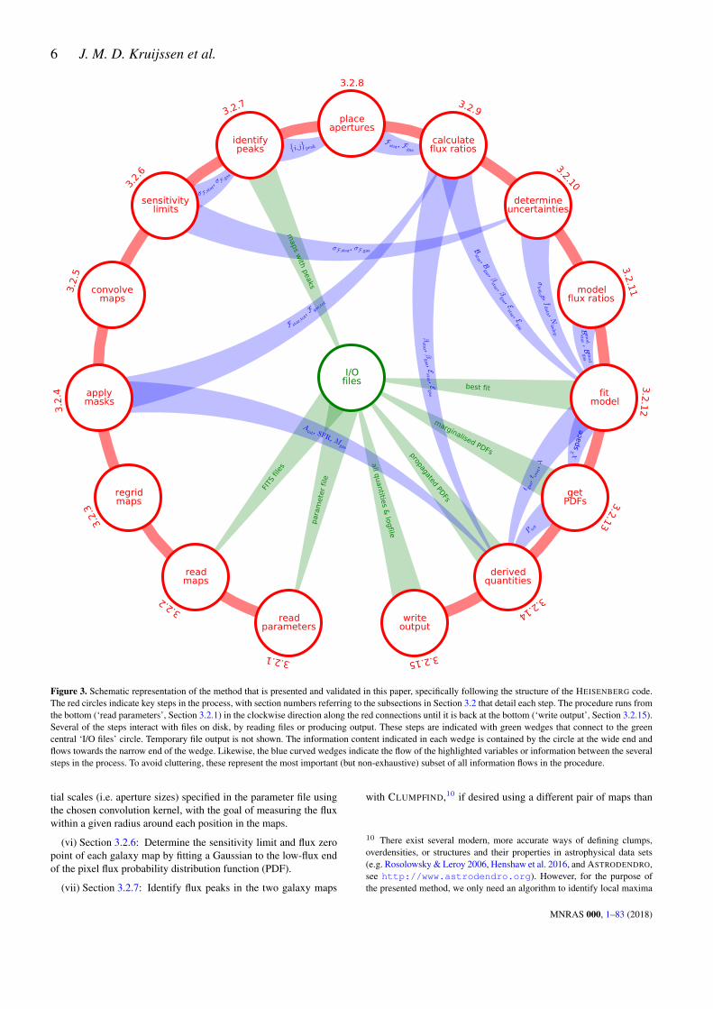
The practical application of the above five steps requires sev-eral additional steps to be taken. Figure 3 shows the structure of theHEISENBERG code, which has been developed for this purpose.Starting from the bottom of the schematic and proceeding in theclockwise direction, the method goes through the following steps(each also listing the subsection numbers in Section 3.2 where thatstep is discussed in detail).
(i) Section 3.2.1: Read in the input parameter file that containsthe settings for carrying out the analysis and use these to derive anyadditional parameters.
(ii) Section 3.2.2: Read in the FITS galaxy maps and determinethe smallest possible aperture size given their spatial resolutions.One of these maps must show a phase from the timeline of Figure 1with a known duration.
(iii) Section 3.2.3: Regrid the galaxy maps by convolving themto the best common spatial resolution and changing the pixel gridto avoid extreme oversampling of a resolution element.
(iv) Section 3.2.4: Apply any masks or cuts in galactocentric ra-dius that are specified in the parameter file to either restrict theanalysis of the galaxy maps to these areas or to omit them from theanalysis.
(v) Section 3.2.5: Convolve the galaxy maps to the range of spa-
MNRAS 000, 1–83 (2018)
6 J. M. D. Kruijssen et al.
F star,t
ot, F ga
s,tot
Atot , SFR, M
gas
σ F,sta
r, σ F
,gas
σF,star, σF,gas
{i,j}
peak
maps w
ith peaks
Fstar, Fgas
Bstar , B
gas , βstar , β
gas , Estar , E
gas
βstar , β
gas , Estar , E
gas
σlog
10 B , fdata , N
indep
Bm
odstar , B
mod
gas
χ2sp
ace
t gas
, tov
er, λ
best fit
P tot
marginalised PDFspropagated PDFs
all q
uantitie
s & lo
gfile
para
mete
r file
FITS
file
s
readparameters
3.2.1
readmaps
3.2.2
regridmaps
3.2.
3
applymasks
3.2
.4
convolvemaps
3.2
.5
sensitivitylimits
3.2.
6identifypeaks
3.2.7
placeapertures
3.2.8
calculateflux ratios
3.2.9
determineuncertainties
3.2.10
modelflux ratios
3.2
.11
fitmodel
3.2
.12
getPDFs 3.2.13
derivedquantities
3.2.14
writeoutput
3.2.15
I/Ofiles
Figure 3. Schematic representation of the method that is presented and validated in this paper, specifically following the structure of the HEISENBERG code.The red circles indicate key steps in the process, with section numbers referring to the subsections in Section 3.2 that detail each step. The procedure runs fromthe bottom (‘read parameters’, Section 3.2.1) in the clockwise direction along the red connections until it is back at the bottom (‘write output’, Section 3.2.15).Several of the steps interact with files on disk, by reading files or producing output. These steps are indicated with green wedges that connect to the greencentral ‘I/O files’ circle. Temporary file output is not shown. The information content indicated in each wedge is contained by the circle at the wide end andflows towards the narrow end of the wedge. Likewise, the blue curved wedges indicate the flow of the highlighted variables or information between the severalsteps in the process. To avoid cluttering, these represent the most important (but non-exhaustive) subset of all information flows in the procedure.
tial scales (i.e. aperture sizes) specified in the parameter file usingthe chosen convolution kernel, with the goal of measuring the fluxwithin a given radius around each position in the maps.
(vi) Section 3.2.6: Determine the sensitivity limit and flux zeropoint of each galaxy map by fitting a Gaussian to the low-flux endof the pixel flux probability distribution function (PDF).
(vii) Section 3.2.7: Identify flux peaks in the two galaxy maps
with CLUMPFIND,10 if desired using a different pair of maps than
10 There exist several modern, more accurate ways of defining clumps,overdensities, or structures and their properties in astrophysical data sets(e.g. Rosolowsky & Leroy 2006, Henshaw et al. 2016, and ASTRODENDRO,see http://www.astrodendro.org). However, for the purpose ofthe presented method, we only need an algorithm to identify local maxima
MNRAS 000, 1–83 (2018)

Cloud-scale star formation across cosmic history 7
those used in the multi-scale flux integration, omit peaks with totalfluxes below the sensitivity limit or those that should be excludeddue to the area masking, and output images of the maps highlight-ing the positions of the included peaks.
(viii) Section 3.2.8: Calculate the fluxes within the apertures ofvarying size focused on each peak, as well as the effective aper-ture size and areas accounting for masked pixels, and the distancesbetween all possible peak pairs.
(ix) Section 3.2.9: Calculate the flux ratio ‘bias’ (i.e. excess ordeficit) relative to the galactic average for each set of peaks as inthe tuning fork diagram of Figure 2. For each aperture size andwithin apertures focused on each of the two sets of flux peaks, firstcalculate the total flux enclosed by the apertures in each of the twomaps. This results in four total fluxes per aperture size: the flux inthe first/second map around the peaks identified in the first/secondmap. For each aperture size and peak type, these fluxes are obtainedby drawing Monte-Carlo realisations of peak subsets that have non-overlapping apertures, to ensure no pixels are counted twice, and bythen taking the mean of the resulting total fluxes across all realisa-tions. The flux ratio excess (i.e. the top branch from Figure 2) thenfollows by taking the peak sample from the first map and divid-ing the total flux around these peaks in the first map by that in thesecond map. The flux ratio deficit (i.e. the bottom branch from Fig-ure 2) then follows by taking the peak sample from the second mapand dividing the total flux around these peaks in the first map bythat in the second map. These flux ratio biases are then normalisedby the average flux ratio between both maps across the entire field.
(x) Section 3.2.10: Determine the uncertainties on the observedflux ratio bias measurements. The sources of uncertainty thatshould be considered are the sensitivity limits of the maps, whichleads to flux uncertainties, and the variety of region masses, whichmanifests itself as a non-zero variance of the fluxes in individualapertures. Because the data points are flux ratios and thus originatefrom two fluxes, it is necessary to subtract the covariance betweenthe numerator and the denominator, which reflects spatial trends inregion properties. Finally, the uncertainty on each individual datapoint differs from the effective error bar when fitting a model to thedata points, because the data points are not independent betweendifferent aperture sizes. Each data point on a branch in the tuningfork (Figure 2) represents a different aperture size that is centredon the same set of peaks, implying that larger apertures (partially)contain the same flux as smaller apertures. We account for this bycalculating the ‘independence fraction’ of each data point relativeto all other data points.
(xi) Section 3.2.11: Derive a model that connects the flux ratiobiases in the tuning fork diagram of Figure 2 to the evolutionarytimeline of Figure 1. Such a model was presented in KL14, whichconsidered a random distribution of point-like regions that are sit-uated at random positions on the evolutionary timeline and also al-lowed these regions to undergo flux evolution between the overlap-ping and ‘isolated’ phases in Figure 1. However, practical applica-tions of this model also require it to deal with regions of finite den-sities, i.e. regions characterized by extended emission rather thanpoint particles. The present paper greatly improves on KL14 byassuming that the regions follow a certain spatially-extended pro-file and then using the flux density contrast between the peaks and
in two-dimensional maps. These peak coordinates should be measured re-liably, but we do not use the clump properties derived by CLUMPFIND forany important steps in the analysis. This is a relatively simple task for whichthe results provided by CLUMPFIND are entirely adequate.
their immediate surroundings to determine the characteristic sizesof these regions in units of the region separation length.
(xii) Section 3.2.12: Carry out a reduced-χ2 fit of the model tothe data points and their (independence-weighted) uncertainties todetermine the quantities describing the time-evolution of indepen-dent regions. In the context of Figure 1, we thus constrain the best-fitting values of the lifetime of the first phase tgas (assuming thatthe second phase provides the reference time-scale described inSection 2.2), which in applications to molecular gas maps repre-sents the molecular cloud lifetime, the duration of the overlap phasetover, which in applications to molecular gas and SFR tracer mapsrepresents the feedback time-scale, and the mean separation lengthbetween independent regions λ. Because we carry out a reduced-χ2
fit, the fitting process also returns the three-dimensional PDF of theabove three model parameters. Additional quantities that are alsoreturned by the fitting process (but are not specifically fitted for) areβstar and βgas, which refer to the mean flux ratios of regions resid-ing in the overlap phase relative to their ‘isolated’ phases, i.e. out-side of the overlap phase (see Section 3.3 of KL14). These twoparameters capture the (possibly complex) flux evolution of bothtracers over the evolutionary timeline. This step also generates theoutput tuning fork diagram including the best-fitting model as afigure and as an ASCII table.
(xiii) Section 3.2.13: Get the marginalised, one- and two-dimensional PDFs of each of the (pairs of) three free parametersin the model, i.e. tgas, tover, and λ, and write the resulting figuresand ASCII tables to disk. The error bars on the best-fitting valuesreturned by the procedure refer to the 32nd percentile of the part ofthe one-dimensional PDF below the best-fitting value and the 68thpercentile of the part of the PDF above the best-fitting value.
(xiv) Section 3.2.14: Calculate derived quantities using the fun-damental free parameters tgas, tover, and λ. These quantities arethe total star formation tracer lifetime including the overlap phase(tstar), the total duration of the evolutionary timeline (τ ), the re-gion radii (rstar and rgas), the region size-to-separation ratios orfilling factors (ζstar and ζgas), the feedback outflow velocity (vfb),the field-wide gas depletion time (tdepl), the star formation effi-ciency per star formation event (εsf ), the star formation and massremoval rates per star formation event (Msf and Mfb), the instan-taneous and time-averaged mass loading factors (ηfb and ηfb), andthe feedback energy and momentum efficiencies (χfb,E and χfb,p).The one-dimensional PDFs of each of these quantities are deter-mined using Monte-Carlo error propagation, where we draw fromthe complete, three-dimensional PDF of tgas, tover, and λ obtainedfrom the fitting process as well as from the PDF of any other, inde-pendent quantities that are used to derive the above quantities. Thistypically leads to well-defined, nearly-noiseless cumulative PDFs.As in the previous step, each of the resulting PDFs are written todisk as figures and ASCII tables.
(xv) Section 3.2.15: Write the output files as ASCII tables thatsummarise all constrained quantities and their error bars, as wellas the logfile containing all of the command line analysis output.These are critical for evaluating and interpreting the results.
The above steps can be carried out on modern personal com-puters or laptops within a reasonable computing time. On such sys-tems, we have achieved typical runtimes of 1–20 minutes per ex-periment, both for the experiments carried out in this paper and forthe first applications of this method (Kruijssen et al. 2018; Haydonet al. 2018; Hygate et al. in prep.; Schruba et al. in prep.; Chevanceet al. in prep.; Ward et al. in prep.). This means that the method can
MNRAS 000, 1–83 (2018)

8 J. M. D. Kruijssen et al.
readily be applied to observational and numerical data sets withoutrequiring special-purpose hardware or supercomputing time.
3.2 Detailed description of the method
We now turn to a detailed description of the method summarisedin Section 3.1 and Figure 3. In this procedure, we extract the quan-tities describing the time evolution of Figure 1 from two galaxymaps that each show the emission from one phase in the timeline.For simplicity and clarity, we assume in this description that oneof the two maps shows molecular gas traced by CO (referred to as‘gas’) and the other shows star formation traced by Hα (referred toas ‘stars’ or ‘stellar’, even though it should technically be ‘youngstars’ or ‘massive stars’). Of these two maps, the stellar phase hasa known duration and therefore acts as a ‘reference time-scale’ thatsets the absolute scale of the entire timeline of Figure 1 – stellarpopulation synthesis models show that the Hα line is emitted overa 5 Myr time-scale (Haydon et al. 2018). Even though this partic-ular example is used here, we expressly reiterate that the methodis capable of handling any pair of emission maps that representcausally-related phases in a Lagrangian timeline as shown in Fig-ure 1. Other examples of tracers that could be used are atomic gas(i.e. HI), dense gas (e.g. traced by HCN), 24 µm emission, ion-ized emission line tracers (e.g. [OIII] or [NII]), or UV emission,but these are by no means exhaustive.11
3.2.1 Input parameters
In order to carry out the analysis depicted in Figure 3, we mustfirst specify a set of flags and input parameters. These are listed inTables 1 and 2, respectively, and are listed in an input parameterfile that is read by the HEISENBERG code. Focusing first on Ta-ble 1, the flags are divided into four main categories, separated bywhite space in the table. The first category concerns optional codemodules or steps, the second enables the use of ancillary maps forcarrying out the peak identification, the third covers the masking-related options, and the fourth lists the analysis options. Table 1highlights the default choice of each of these flags, which will beused throughout the paper unless stated otherwise.
While the descriptions of the flags in Table 1 are mostly self-explanatory, we should comment in some detail on a subset forwhich the choice between the available options may not be obvious.
(i) The tophat flag enables the use of either a two-dimensionalGaussian or tophat kernel to convolve the maps to larger aperturesizes. Technically, only the tophat kernel does this correctly – foreach pixel, it adds up all flux within the specified aperture areacentred on that pixel. The Gaussian kernel adds up the surroundingflux too, but weighs it by a Gaussian profile. We do not use thiskernel in the present paper, because it under-represents the distantpixels within the specified aperture size, but leave it as an availableoption for future work.
(ii) The loglevels flag specifies whether the contour lev-els that are used to identify peaks with CLUMPFIND are equally-spaced in linear or logarithmic space. In principle, there is no cor-rect choice – it depends on the maps to be analysed which optionbest identifies peaks of interest. Some trial-and-error is necessar-ily involved. However, given that the mass functions of molecu-lar clouds and stellar clusters are characterized by power laws (see
11 Applications of the presented method to a wide variety of different trac-ers in the Large Magellanic Cloud will be presented by Ward et al. in prep.
e.g. the reviews by Portegies Zwart et al. 2010; Dobbs et al. 2014;Kruijssen 2014), we prefer using logarithmically-spaced contourlevels. As demonstrated below, this results in a satisfactory identi-fication of peaks in the maps used in this paper.
(iii) The flux weight flag enables the peak position to cor-respond to the brightest pixel or the flux-weighted mean within thepeak area. The latter option uses the area of the peak as defined byCLUMPFIND. Because there is no obvious physical definition of thepeak edge (and hence its area), we prefer to use the brightest pixel.
(iv) The tstar incl flag indicates whether, in the context ofthe evolutionary timeline shown in Figure 1, the specified ‘ref-erence’ time-scale tstar,ref (see Section 2.2) includes the overlapphase (with duration tover) or not. This depends entirely on the trac-ers used. In the present paper, we use pairs of maps generated fromgalaxy simulations. These map pairs can consist of two stellar mapscovering star particles with two different, specified ranges of ages(used to test whether the method retrieves the correct evolution-ary timeline, see Section 4.2), or of one such stellar map togetherwith a gas map (used to correct the accuracy of the method undera variety of observational conditions, see Section 4.3). In the caseswhere we use pairs of stellar maps, the reference time-scale in-cludes the time overlap with the other stellar map. However, whenusing a stellar map and a gas map, the reference time-scale doesnot include this overlap phase, because new star particles may formas long as a region still contains gas. Similar considerations willhold in observational applications. When applying the presentedmethod to measure a molecular cloud lifetime as traced by CO andusing an ionized emission line like Hα or broadband UV to tracestar formation, it is reasonable to assume that the correspondingreference time-scale does not include the overlap phase. Hα andUV emission trace unembedded, massive stars, which locally haveblown out the residual gas while massive star formation may stillbe ongoing in other parts of the star-forming region (e.g. Ginsburget al. 2016). The emission lifetimes of SFR tracers such as Hα andFUV or NUV are set by stellar population synthesis models, whichassume a coeval stellar population (Haydon et al. 2018, also seeLeroy et al. 2012), and therefore do not include the time tover dur-ing which stars may still be forming – the clock starts ticking whenthere is no molecular gas left.
Turning to the description of the input parameters in Table 2,there are six main categories, again separated by white space inthe table. The first category contains quantities describing the basicgalaxy properties and manipulation of the maps, the second cov-ers the definition of the aperture sizes to be used in the analysis,the third concerns the peak identification, the fourth describes thequantities needed to define the evolutionary timeline, the fifth setsthe parameters for carrying out the fit of our model to the data, andthe sixth lists conversion factors and constants needed to calculatethe derived physical quantities discussed in Sections 3.2.14 and 5.
As before, many of the input parameters in Table 2 are self-explanatory, but we will discuss a subset of twelve items for whichthe choice of value is non-trivial.
(i) The parameters Rmin and Rmax can be chosen to limit theanalysis to a certain galactocentric radial interval within a galaxy (ifcut radius = 1), which can be of great interest when studyingany of the quantities constrained by our method, e.g. the molecularcloud lifetime, star formation efficiency, or outflow velocity. How-ever, care must be taken that the radial interval does not becometoo narrow, i.e. when the area contains too few peaks (this state-ment is quantified in Section 4.3.8) or that it limits the maximumattainable effective aperture size such that the galactic average in
MNRAS 000, 1–83 (2018)

Cloud-scale star formation across cosmic history 9
Table 1. Flags to be set for the presented analysis
Flag Values (default) Description
mask images 0/1 Mask images (off/on)generate plot 0/1 Generate output plots and save to PostScript files (off/on)derive phys 0/1 Calculate derived physical quantities as described in Section 3.2.14 (off/on)write output 0/1 Write results to output files (off/on)
use star2 0/1 Use a second map for identifying stellar peaks and use the default map for performing the flux calculation (off/on)use gas2 0/1 Use a second map for identifying gas peaks and use the default map for performing the flux calculation (off/on)
mstar ext 0/1 Mask areas in stellar map exterior to regions listed in a specified DS9 region file (off/on)mstar int 0/1 Mask areas in stellar map interior to regions listed in a specified DS9 region file (off/on)mgas ext 0/1 Mask areas in gas map exterior to regions listed in a specified DS9 region file (off/on)mgas int 0/1 Mask areas in gas map interior to regions listed in a specified DS9 region file (off/on)cut radius 0/1 Mask maps outside a specified radial interval within the galaxy (off/on)
set centre
{0 Pixel coordinates of the galaxy centre are set to the central pixel of the map1 Specify pixel coordinates of the galaxy centre (default)
tophat?{
0 Use Gaussian kernel to convolve maps to larger aperture sizes1 Use tophat kernel to convolve maps to larger aperture sizes (default)
loglevels?{
0 Contour levels for peak identification are equally-spaced in linear space1 Contour levels for peak identification are equally-spaced in logarithmic space (default)
flux weight?{
0 Peak positions correspond to brightest pixel in peak area (default)1 Peak positions correspond to flux-weighted mean position of peak area
calc ap area 0/1 Calculate the effective aperture area using the number of unmasked pixels within the target aperture area (off/on)
tstar incl?{
0 Reference time-scale tstar,ref does not include the overlap phase (i.e. tstar = tstar,ref + tover, default)1 Reference time-scale tstar,ref includes the overlap phase (i.e. tstar = tstar,ref )
peak prof
0 Model independent regions as points1 Model independent regions as constant-surface density discs2 Model independent regions as two-dimensional Gaussians (default)
?These flags are discussed specifically in Section 3.2.1. For the other flags, the descriptions in this table are considered to be largely self-explanatory.Examples of setting some of these flags are given in the pertinent subsections below.
Figure 2 cannot be reached. This requires some iteration after thefirst application of the analysis to a particular data set.
(ii) The parameter Nsamp indicates the maximum number ofpixels used to sample the smallest aperture size [which is typicallychosen to match the full width at half maximum (FWHM) of thenative point spread function (PSF), see below] after regridding theinput maps to the same pixel grid. For instance, for the default valueof Nsamp = 10 and a minimum aperture size of lap = 50 pc, themaps will be placed on a grid with lap/Nsamp = 5 pc pixels. Clas-sical Nyquist sampling corresponds to Nsamp = 2.5, which yieldsmaps with a factor of 16 fewer pixels than our default value andtherefore results in improved performance on slow machines. How-ever, we find that this sampling of the aperture size is too coarseto enable the peak identification process to identify all peaks incrowded regions. Setting Nsamp = 10 enables accurate peak iden-tification at an acceptable increase in computing time.
(iii) The parameter θast defines the maximum allowed tolerancebetween the pixel coordinates and pixel dimensions of the maps.After the maps have been regridded to an optimal pixel scale (seeSection 3.2.3), we verify in Section 3.2.4 that the pixel grids arethe same to within θast, based on the pixel coordinates and dimen-sions specified in the headers of the FITS files containing the galaxymaps. We adopt a default tolerance of θast ∼ 10−6 deg ∼ 3 mas,which corresponds to ∼ 0.01 pc in our simulated galaxy maps(D = 840 kpc), to ∼ 1 pc at a distance of D ∼ 60 Mpc, andto ∼ 30 pc at z ∼ 3. This default angle of 3 mas is well belowthe spatial resolution used in this paper or the resolution generallyachieved with modern observatories. This guarantees that the pixelgrid cannot be a source of positioning errors. Of course, this as-sumes that the pixel coordinates specified in the FITS headers are
correct. The astrometric precision of the maps should be verifiedmanually before applying the presented method (see Section 3.2.2).
(iv) The parameter Nbins sets the number of bins that is usedto sample the pixel flux PDF and fit a Gaussian to determine thesensitivity limit of each map. The default number is Nbins = 20,which is somewhat arbitrary but yields accurate results.
(v) The parameters lap,min, lap,max, andNap together define thearray of aperture sizes (i.e. diameters) to which the maps are con-volved and at which the analysis is carried out. Specifically, theapertures are logarithmically spaced, such that:
lap(i) = lap,min
(lap,max
lap,min
) iNap−1
, (3)
with {i ∈ N | 0 6 i 6 Nap − 1}. The desired values of lap,min,lap,max, andNap strongly depend on the problem at hand. The min-imum aperture size lap,min should be similar to the coarsest resolu-tion across both maps, whereas lap,max should be large enough toenable the large-scale convergence of the curves in the tuning forkdiagram of Figure 2 to the galactic average. The choice of maxi-mum aperture size may therefore require some iteration. Likewise,there is no a priori rule for choosing the number of aperture sizesNap. Most importantly, it should be large enough to sample theshape of the curves in the tuning fork diagram. The possible over-sampling of these curves with a large number of aperture sizes (andhence observational data points) is harmless, because the statisti-cal part of our analysis corrects for correlations between the datapoints (see Section 3.2.10). However, using an unnecessarily largenumber of aperture sizes can greatly slow the analysis. Again, someiteration may be required to optimize this choice for the maps underconsideration. For the tests performed in this paper, we find that the
MNRAS 000, 1–83 (2018)

10 J. M. D. Kruijssen et al.
Table 2. Input parameters of the presented analysis
Quantity [unit] Default Description
D [pc] – Distance to galaxyi [◦] 0 Inclination angleφ [◦] 0 Position angleicen [pix] – Index of x-axis coordinate of galaxy centre (only used if set centre = 1, otherwise set to central pixel in map)jcen [pix] – Index of y-axis coordinate of galaxy centre (only used if set centre = 1, otherwise set to central pixel in map)Rmin [pc]? 0 Minimum inclination-corrected radius for analysis (only used if cut radius = 1)Rmax [pc]? 10000 Maximum inclination-corrected radius for analysis (only used if cut radius = 1)Nsamp
? 10 Maximum number of pixels per unit FWHM of a map resolution element after regridding the mapsθast [◦]? 10−6 Allowed tolerance between the pixel coordinates and pixel dimensions in both mapsNbins
? 20 Number of bins used during sensitivity limit calculation to sample the flux PDFs and fit Gaussians
lap,min [pc]? 50 Minimum inclination-corrected aperture size (i.e. diameter) to convolve the input maps tolap,max [pc]? 6400 Maximum inclination-corrected aperture size (i.e. diameter) to convolve the input maps toNap
? 8 Number of aperture sizes used to create logarithmically-spaced aperture size array in the range [lap,min, lap,max]
Npix,min? 20 Minimum number of pixels for a valid peak (use Npix,min = 1 to allow single points to be identified as peaks)
Nσ 5 Flux multiple of the derived sensitivity limit needed for a peak to be included∆ log10 Fstar
? 2 Logarithmic range below flux maximum covered by flux contour levels for stellar peak identificationδ log10 Fstar
? 0.5 Logarithmic interval between flux contour levels for stellar peak identification∆ log10 Fgas
? 2 Logarithmic range below flux maximum covered by flux contour levels for gas peak identificationδ log10 Fgas
? 0.5 Logarithmic interval between flux contour levels for stellar peak identificationNlin,star
? 11 Number of contours for stellar peak identification with range min (Fstar)–max (Fstar) (only used if loglevels = 0)Nlin,gas
? 11 Number of contours for gas peak identification with range min (Fgas)–max (Fgas) (only used if loglevels = 0)
tstar,ref [Myr]? – Reference time-scale spanned by star formation tracerσ−(tstar,ref) [Myr] 0 Downwards uncertainty on reference time-scaleσ+(tstar,ref) [Myr] 0 Upwards uncertainty on reference time-scaletgas,min [Myr] 0.1 Minimum value of tgas considered during fitting processtgas,max [Myr] 3000 Maximum value of tgas considered during fitting processtover,min [Myr] 0.01 Minimum value of tover considered during fitting process
Nmc,peak? 1000 Number of Monte-Carlo realisations of independent peak samples to be generated and averaged over
Ndepth? 4 Maximum number of free parameter array refinement loops for obtaining best-fitting value
Ntry? 101 Size of each free parameter array to obtain the best-fitting value
Nmc,phys? 106 Number of Monte-Carlo draws used for error propagation of derived physical quantities
log10 Xstar? – Logarithm of conversion factor from map pixel value to an absolute SFR in M� yr−1 (only used if derive phys = 1)
σrel(Xstar) 0 Relative uncertainty (i.e. σx/x) of Xstar (only used if derive phys = 1)log10 Xgas
? – Logarithm of conversion factor from map pixel value to an absolute gas mass in M� (only used if derive phys = 1)σrel(Xgas) 0 Relative uncertainty (i.e. σx/x) of Xgas (only used if derive phys = 1)ΨE [m2 s−3]? – Light-to-mass ratio of a desired feedback mechanism (only used if derive phys = 1)ψp [m s−2]? – Momentum output rate per unit mass of a desired feedback mechanism (only used if derive phys = 1)
?These parameters are discussed specifically in Section 3.2.1. For the other parameters, the descriptions in this table are considered to be largelyself-explanatory. Examples of setting some of these parameters are given in the pertinent subsections below.
default values of lap,min, lap,max, andNap provide accurate results.In Section 4.3.6, we vary lap,min and Nap to carry out a resolutiontest and quantify the requirements for observational applications ofthe method.
(vi) The parameter Npix,min represents the minimum area of apeak identified by CLUMPFIND (see Figure 2 of Williams et al.1994) to be considered in the remainder of the analysis. The de-fault value of Npix,min = 20 avoids unreliable detections with-out obstructing the identification of unresolved point sources. Forillustration, the default pixel sampling rate Nsamp = 10 meansthat the typical area within an FWHM is 75 pixels, implying that aminimum area of 20 pixels enables the identification of unresolvedpoint sources. To apply the analysis to maps of point-like regions(see Section 4), it is necessary to set Npix,min = 1.
(vii) The parameters ∆ log10 F and δ log10 F (with subscripts‘star’ and ‘gas’ referring to stars and gas, respectively) set thelogarithmic range and separation of the contour levels used byCLUMPFIND to identify peaks (see Section 3.2.7 for a summaryof how this identification is performed, or Williams et al. 1994 for
a detailed discussion). Choosing the best values of these param-eters requires the visual inspection of the maps produced by theanalysis (see Figure 3). If faint but relevant peaks are not identified,∆ log10 F should be increased, whereas it should be decreased ifspurious peaks are identified. If adjacent but independent peaks arenot distinguished, one should decrease δ log10 F , whereas it shouldbe increased if multiple peaks within a single independent regionare each identified individually. Lacking a quantitative definitionof ‘independent regions’ other than the idealised description givenin Section 2.1, these choices are necessarily somewhat arbitrary.However, the details of the peak identification do not strongly af-fect the constrained quantities as long as an ‘obvious’ set of phys-ically relevant peaks is identified, because we carry out Monte-Carlo sampling of peaks to discard close pairs (see below and Sec-tion 3.2.8). The default values of ∆ log10 F and δ log10 F providea good starting point for applications of the method and are usedfor most of the experiments discussed in this work. The same ap-proach applies to the choice of Nlin,star and Nlin,gas. These quan-tities define the contour level spacing if linearly-spaced contours
MNRAS 000, 1–83 (2018)

Cloud-scale star formation across cosmic history 11
are chosen (i.e. loglevels = 0) and should be chosen by visualinspection of the maps produced by the analysis. In general, it isimportant to realise that the peak identification should have accessto most of the tracer emission in the maps. If the peak positions ofeither tracer are biased to areas of the map that do not host most ofthe tracer emission, e.g. due to differences in spatial structure andclumpiness, this negatively affects the accuracy of the method.
(viii) The parameter tstar,ref represents the ‘reference time-scale’ that is used to translate the derived relative evolutionarytimeline to an absolute one (cf. Figure 1). Throughout this paper,we assume that tstar,ref refers to the SFR tracer map, because stellarpopulation synthesis models like STARBURST99 (Leitherer et al.1999) can provide an absolute ‘lifetime’ for the emission from mas-sive stars. Although the characteristic lifetimes of SFR tracers suchas Hα, FUV, and NUV can vary by more than an order of mag-nitude depending on the definition used (Leroy et al. 2012, Table3), they have been calibrated specifically for use in the presentedmethod by Haydon et al. (2018), who also considered the effect ofsampling from the initial mass function (IMF) in low-SFR envi-ronments. These lifetimes are the best choice for observational ap-plications of the method. Of course, once the lifetime of any othertracer (e.g. CO) in the galaxy under consideration has been mea-sured using our method, it becomes possible to use that lifetimeas a reference time-scale for other measurements. In the specificcontext of our tests of the method using galaxy simulations in Sec-tion 4, we use maps of the star particles in specific age bins, whichgrants us full control over the value of tstar,ref .
(ix) The parameter Nmc,peak denotes the number of Monte-Carlo experiments used to draw independent peak samples fromthe parent sample at each aperture size. In other words, we gener-ateNmc,peak different (but inevitably partially overlapping) subsetsof peaks such that none of these peaks has any neighbours withinlap. As described in Section 3.1, this is a necessary step to makesure that flux around peaks in crowded regions is not counted morethan once. The total gas and stellar fluxes around each peak type(i.e. gas peaks in the top branch of Figure 2, as well as stellar peaksin the bottom branch) are then averaged over the Nmc,peak experi-ments. Setting Nmc,peak too low can result in run-to-run variationsof the data points and thus the best-fitting quantities. It is thereforeimportant to choose a sufficient number of Monte-Carlo samples,even if this goes at the expense of computing time (which scales asN2
mc,peak due to looping over all peak pairs). We find that at the de-fault Nmc,peak = 1000, the run-to-run variation is of the order 1–2per cent, which is appreciably smaller than the uncertainties on thebest-fitting quantities. This value requires a few minutes of runtimeon modern laptops and is therefore used throughout the paper.
(x) The parameters Ndepth and Ntry govern the fitting process.This part of the analysis takes up a significant fraction of the com-puting time and can even dominate altogether. As discussed in Sec-tion 3.1, we carry out the fit in a three-dimensional parameter spaceof tgas, tover, and λ. To achieve a reasonable computing time with-out sacrificing precision, we therefore iteratively refine the fittinggrid by zooming in on the best-fitting point in parameter space. Theparameter Ndepth sets the maximum number of refinement steps(see Section 3.2.12 for details) andNtry sets the number of array el-ements in each of the three free parameters that is evaluated duringeach refinement step, resulting in a total number of N3
try elements.This third-power scaling of the total number of elements meansthat it is very important to optimize the choice of Ndepth and Ntry.For the default values of Ndepth = 4 and Ntry = 101, we obtainwell-converged results within a reasonable runtime, to the extent
that Ndepth is typically not even reached because the condition forconvergence is already satisfied during an earlier refinement step.
(xi) The parameter Nmc,phys sets the number of Monte-Carlodraws used to perform the error propagation for the derived quan-tities in Section 3.2.14. Again, this process can be quite time-intensive, implying that there is a trade-off between runtime andthe smoothness of the PDFs of the derived physical quantities. Forthe default value of Nmc,phys = 106, the noise on the PDFs of thederived quantities is effectively unnoticeable, whereas it is entirelyabsent in the cumulative distribution functions (CDFs). To mini-mize the computing time, Nmc,phys can be lowered by up to twoorders of magnitude, resulting in PDFs that have noticeable noise,but CDFs that are still smooth and well-defined. Throughout thepaper, we adopt the default value listed in Table 2.
(xii) The parameters log10 Xstar and log10 Xgas represent thelogarithm of the conversion factors from a pixel value to an abso-lute SFR (in M� yr−1) and an absolute gas mass (in M�), respec-tively. Their values account for the conversion of the input maps’flux units to the physical units adopted in HEISENBERG. As such,log10 Xstar and log10 Xgas depend on the units of the maps un-der consideration as well as the distance of the galaxy, implyingthat these parameters need to be calculated prior to applying themethod to a certain data set. The native input maps considered inthe present paper show gas and stellar surface densities on a pixelscale of ∆x = 14.25 pc (see Section 4), which means that theconversion factor to an SFR is given by
log10 Xstar = log10
[(∆x
pc
)2(tstar
yr
)−1], (4)
where the division by the stellar lifetime is necessary to convert astellar surface density in a known age bin to a corresponding time-average SFR. For the experiments in this paper, assuming a valueof tstar = 1 Myr would imply log10 Xstar = −3.692. Likewise,the conversion factor to a gas mass is given by
log10 Xgas = log10
[(∆x
pc
)2], (5)
which for the experiments in this paper becomes log10 Xgas =2.308. These conversion factors are updated whenever the mapsare regridded to a different pixel scale. Note that other data sets willrequire other expressions and values. The above examples are in-tended to illustrate the definition of these conversion factors. Also,we emphasize that the conversion factors are only used when calcu-lating the derived physical quantities in Section 5. The KL14 prin-ciple itself and the associated method to constrain the evolutionarytimeline of Figure 1 both rely on flux ratios relative to the galacticaverage, implying that the conversion factors cancel.12
(xiii) Finally, the parameters ΨE and ψp are the light-to-massratio (or energy injection rate per unit mass) and momentum out-put rate per unit mass, respectively. They are only used when cal-culating the feedback energy and momentum efficiencies in Sec-tion 5, which is done by comparing the effective output energy andmomentum injection rates constrained by the method to the totalrates implied by the young stellar populations in the star-formingregions. These parameters are needed to derive the total injectionrates – their values depend on the feedback mechanism under con-sideration and the time-scale over which the rates are averaged. For
12 This only holds if the conversion factors do not vary across the map. SeeSection 3.2.2 for a discussion of ways to apply the method to galaxies withnon-uniform conversion factors.
MNRAS 000, 1–83 (2018)

12 J. M. D. Kruijssen et al.
most feedback mechanisms, suitable numbers for these quantitiescan be obtained from stellar population synthesis models (e.g. Lei-therer et al. 1999; Agertz et al. 2013).
All flags and input parameters are specified in an input file,which is read in by HEISENBERG. Next to the elements listed inTables 1 and 2, it also contains the full path of the maps and anyDS9 region files used in the analysis to mask the maps.13 In addi-tion, the input file includes a small number of quantities that are notlisted in Tables 1 and 2 because they are not relevant to the presentpaper, but are required to run the analysis. They are included in theHEISENBERG documentation when it is made publicly available.
3.2.2 Selecting and reading in galaxy maps
The next step in the analysis process is to read in the galaxy mapsin FITS format to which the method is applied. In Section 3.1, weexplained that these maps can show any tracer pair of interest thatfollows a Lagrangian evolutionary connection as in Figure 1. Asstated previously, here we follow an example case in which ‘gas’turns into (young) ‘stars’, but we reiterate that the presented methodapplies much more generally.
Irrespective of their physical nature, the pair of maps shouldsatisfy a number of conditions.
(i) The maps should be two-dimensional and share the same di-mensions and pixel grid. In the case of a spectral cube containingline emission data, this means one should use a moment-0 map.The pixel grid is defined using pixel coordinates {i, j}, with {i ∈N | 0 6 i 6 Npix,x−1} and {j ∈ N | 0 6 j 6 Npix,y−1}, where{Npix,x, Npix,y} represent the number of pixels in the {x, y} di-rections. The pixel values represent the stellar and gas flux densitiesFstar,ij and Fgas,ij , respectively.
(ii) The astrometric precision of the pair of maps should be suf-ficient, such that positional uncertainties are considerably smallerthan the resolution FWHM. The presented method correlates thespatial structure in pairs of tracer maps to derive the underlyingevolutionary timeline. It therefore relies strongly on accurate posi-tion information. We have quantified this by carrying out experi-ments with a positional offset in one of the maps, which show thatan acceptable astrometric precision is ∼ 1/3 of the FWHM. Thisis commonly achieved with modern observatories, which routinelyachieve astrometric precision of the order of 10 per cent of theFWHM or better. For instance, ALMA achieves a precision of 0.05times the FWHM, with a minimum of 3 mas.14 Maps for which theastrometric uncertainty exceeds 1/3 of the FWHM cannot be usedfor measuring tover, because such large positional offsets prohibitthe statistical identification of physically co-spatial regions in bothmaps. If the astrometric uncertainties are not much smaller than theFWHM, the duration of the overlap phase tover (see Figure 1) willbe underestimated.
(iii) One has to be relatively confident that each cloud or star-forming region that is visible in one tracer is also visible in theother tracer at some point in its lifecycle. The constrained lifetimes
13 To create the DS9 region files used for masking (see below), DS9 isavailable at http://ds9.si.edu. In addition, DS9 region files maybe created manually, using the region file description that can be found athttp://ds9.si.edu/doc/ref/region.html.14 See the ALMA Technical Handbook at https://almascience.eso.org/documents-and-tools/.
are a population average over all regions, meaning that if this con-dition is not satisfied, the lifetime includes a zero-duration contri-bution from those regions that never appear in one of the tracers.However, it does not necessarily pose a problem if regions neverappear in either tracer, because then they are simply omitted fromthe population-average evolutionary timeline altogether. In such acase, the method returns the ‘visibility time-scale’ and ‘visible sep-aration length’ of the tracers. The retrieved time-scales still matchthe ‘true’ underlying lifetimes if the number of invisible regions issmall or these regions are consistent with being a randomly drawnsubset of the parent population. There are no general guidelinesfor dealing with region visibility, because its implications dependsstrongly on the question at hand and the tracers used. Specific ex-amples are discussed in Sections 4.3.3 and 7.2.2.
(iv) Contamination should be minimized such that the emissionfrom each tracer can be considered to be almost exclusively as-sociated with the physical objects of interest. In the case of Hαemission, one would want to avoid emission from shock-heatedgalactic accretion or outflows that are not driven by stellar feed-back. Likewise, 24µm emission may trace both young and evolvedstars, which complicates its interpretation as a star formation tracer.In general, diffuse emission due to unresolved, low-mass objectsor photon scattering at large distances from the emission sourcesshould be removed from the maps. Ideally, this filtered emission isadded back into the image by rescaling the pixel values. The mainreason for filtering diffuse emission is that it does not belong tothe population of peaks that is being studied. In extreme cases, thepresence of a large flux reservoir without peaks in one of the tracerscan result in a tracer deficit relative to the galactic average when fo-cusing on the corresponding tracer peaks, because the diffuse fluxcontributes to the galactic average without contributing to the fluxaround the identified peaks (see Section 4.3.9 for a detailed dis-cussion). This should be avoided. A new module in HEISENBERG
has the purpose of automatically filtering out diffuse emission (Hy-gate et al. 2018), but if this module is not used, the maps should bevisually inspected and pre-processed if necessary.
(v) The emission maps should be as homogeneous as possi-ble, avoiding major variations of extinction, excitation conditions(e.g. temperature), and chemical abundances across the consideredarea. In principle, it is one of the method’s main strengths that itis insensitive to galaxy-to-galaxy variations of the uncertain con-version factors between gas tracer flux and the gas mass that arewell-known to hamper studies of extragalactic star formation (e.g.Daddi et al. 2010). However, if these quantities do vary stronglywithin a map (e.g. in the case of radial gradients in galaxies), thismay pose a problem. In that case, one can still apply the method,but it should be acknowledged that a tracer lifetime will be obtainedunder the population-average conditions of the varying quantity. Ifthis is undesirable (e.g. due to a spatially-varying CO-to-H2 con-version factor), it is recommended to either apply this conversionfactor to the map beforehand, or to apply the method separately toradial bins in which any variation is within acceptable limits.
(vi) The sensitivities or detection limits of the maps should en-able a representative fraction of the tracer emission of interest to berecovered.
(vii) The spatial resolution of the maps should enable the char-acteristic separation length between independent regions λ to beresolved. This can only be verified after applying the method andis discussed in detail in Section 4.3.6.
(viii) The largest effective aperture size (after subtracting anymasked pixels from the aperture) should enable the convergencetowards the galactic average in Figure 2 to be reached. If this is
MNRAS 000, 1–83 (2018)

Cloud-scale star formation across cosmic history 13
not achieved, any masks or limits on the range of galactocentricradii should be relaxed to increase the largest effective aperturesize. Should the galactic average still not be retrieved in any cir-cular aperture (this is possible for irregular fields), the individualmaps may be unsuitable for applying the method. The method maystill be applied to such galaxies by combining the images of multi-ple galaxies at the same physical scale side-by-side in a single map,or combining the peak samples obtained for the individual galax-ies, as long as these combinations are carried out prior to fitting themodel. In this case, the method constrains the population-averageevolutionary timeline of Figure 1 for the combined galaxy sample.
(ix) If one wishes to recover absolute time-scales, then the life-time of the tracer shown in one of the maps must be known, eitherdirectly from stellar population synthesis modelling (e.g. when us-ing Hα, FUV, or NUV, see Haydon et al. 2018), or by having beencalibrated to such a reference time-scale in a separate application ofthe method. In other words, if the CO lifetime has been measuredby applying the method to an Hα map and a CO map, then eitherof these can be used as a reference time-scale when measuring thelifetimes of HI clouds across the same area.
While it may seem that the above points set stringent limits on theapplicability of the method, there currently exists a broad rangeof observational data sets that satisfy these conditions. These con-ditions are merely intended as guidelines to carefully considerwhen selecting the maps. In general, the KL14 principle shouldbe thought of as a purely empirical method that as such will notnecessarily yield a ‘wrong’ answer if any of the above conditionsare violated. However, the choice of maps and their properties to-gether define the question that is answered by applying the method.Therefore, the interpretation of the results depends on to what ex-tent these guidelines for selecting the maps are satisfied. In prac-tice, some of the above guidelines cannot be evaluated in advance(e.g. points vii and viii) and must be addressed a posteriori, after theanalysis with HEISENBERG is completed. The above list should beevaluated in addition to the guidelines for observational applica-tions from Section 4.4. We note that all of the above conditions aresatisfied by the simulated maps that are used in this paper.
It is possible to select different maps for the peak identifica-tion and for the flux integration. An example where this may beof interest is when using CO(1–0) observations to trace molecu-lar gas. These position-position-velocity data cubes can be quitenoisy, meaning that a signal-masked moment-0 map showing onlythe emission above a minimum signal-to-noise level is often neededto select the real peaks in the map and avoid selecting noise peaks.However, this omits real flux from the map, because part of theemission below the signal-to-noise threshold is real. In this case,it may be desirable to use a different map that does include thisemission when calculating the fluxes in the apertures focused oneach peak. For instance, a moment-0 map that is generated with-out a signal-to-noise threshold, but instead uses a certain velocitymask around the velocity field of atomic gas (if available) may helpto include and isolate all real CO emission even in the presence ofnoise. A flux calculation based on such a map would be accurate onscales larger than a few times the PSF, because the noise maximaand minima should then statistically cancel.
Given a selected set of maps, HEISENBERG reads in the FITSfiles. Throughout the description of the method, we will use a pairof example maps to illustrate the application of the method. Theseare taken from the high-resolution, extended emission simulatedmaps of experiment ID 37 in Section 4.3. We describe later howthese particular maps were generated – at this point of the paper,
Gas mapSFR map
5 kpc
Figure 4. Example of two simulated galaxy maps (the high-resolution,extended-emission versions of experiment ID 37 in Section 4.3) that areused for illustrating the method throughout this section. Shown are the SFR(left) and gas (right) maps on a logarithmic stretch over three orders of mag-nitude. The spatial scale is indicated by the scale bar at the bottom.
they exclusively serve an illustrative purpose. The maps are pre-sented in Figure 4 and represent the input for later illustrations ofthe analysis. When reading in the maps, HEISENBERG immediatelyapplies individual masks ξstar,ij and ξgas,ij according to the DS9region files that are specified for each of them. These region filesmay be composites of any number of sub-regions and can be usedto either include or exclude any pixels of which the pixel centresreside within the area enclosed by the region files. The values ofexcluded pixels are set to NaN in each individually-masked map.The synchronisation of each of these masks across all maps is de-ferred to a later step, in which any cuts in galactocentric radius arealso applied (see Section 3.2.4).
After reading in the input file as described in Section 3.2.1and subsequently reading in the maps, their FITS headers, and theDS9 region files, the analysis is self-contained and does not re-quire reading any further files. Before continuing the analysis, wecompare the PSF sizes and determine the largest PSF size lPSF,max
across the set of maps. Assuming a Gaussian PSF, this size corre-sponds to an FWHM. Given the grid of aperture sizes lap definedby the input file and provided in equation (3), we determine theaperture size that is closest to the maximum PSF size in logarith-mic space, i.e. we minimize the quantity | log10(lap/lPSF,max)|,and set lap,min to the aperture size where this minimum is reached.This ensures that we only consider aperture sizes that are at leastmarginally resolved in both of the maps.
3.2.3 Regridding the galaxy maps
The runtime of the analysis increases with the area of the mapsin units of square pixels. For this reason, we regrid the galaxymaps to a smaller number of pixels if the original pixel size lpix
allows doing so. As discussed in Section 3.2.1, the target pixel sizeis lap,min/Nsamp, which ensures that resolution elements are re-solved by a sufficient number of pixels to reliably identify emis-sion peaks. We therefore regrid the maps if the target pixel sizelap,min/Nsamp > 1.2lpix, where the factor of 1.2 is added to skipthe regridding if this yields less than a 30 per cent decrease of themap area in units of square pixels. In addition, the maps are con-volved with a two-dimensional Gaussian PSF to a common res-olution of lap,min, provided that lap,min > 1.05lPSF. Again, thefactor of 1.05 is added to skip the convolution if only a 5 per centchange of resolution would be achieved. If the beam is non-circular,we use the effective beam width lPSF = (lPSF,alPSF,b)
1/2, wherelPSF,a and lPSF,b indicate the beam width along the semi-minor
MNRAS 000, 1–83 (2018)

14 J. M. D. Kruijssen et al.
and semi-major axes, respectively. The convolution of the mapsthen proceeds with a kernel FWHM of (l2ap,min − l2PSF)1/2, whichensures that the final resolution equals lap,min irrespective of theoriginal circular PSF size. The FITS header is updated with the newmap dimensions {Npix,x, Npix,y}, coordinates of the galactic cen-tre {icen, jcen} (which are taken to correspond to the central pixelof the image if set centre = 0), and pixel size θpix. Finally, theupdated FITS file is written to disk for later use. The above proce-dure is applied to each of the maps under consideration.
After the regridding is completed, we update several of thequantities needed for the remainder of the analysis.
(i) The original position of the galactic centre pixel {icen, jcen}is converted to a fraction of the dimensions of the original mapsin units of pixels {Npix,x, Npix,y}. Interpolation of the pixel di-mensions of the regridded maps then provides the position of thecentral pixel in the new maps and thus updates the original valuesof {icen, jcen}.
(ii) The pixel size in pc is determined from the angular size θpix
in the FITS file header of the regridded map by writing
lpix =D tan θpix√
cos i, (6)
where the square root in the denominator accounts for the fact thata non-zero inclination only affects one of the pixel dimensions andthus does not enter linearly in the effective pixel size. If the dis-tance or inclination angle are poorly constrained, we recommendcarrying out the analysis for a reasonable range of distances or in-clination angles to probe the impact of their uncertainties on theinferred quantities.
(iii) We check that there are at least two elements in the aper-ture size array lap that exceed the pixel diagonal
√2lpix to enable
a numerically (but not necessarily physically) meaningful applica-tion of the method. If this is not satisfied, the analysis is stopped tomodify the grid of aperture sizes to increase lap. This can happenif Nsamp <
√2 and the dynamic range of lap is too small, or if the
original pixel size was too large to enable regridding.(iv) If the smallest aperture size lap,min is smaller than the pixel
diagonal, lap,min is changed to the first element of lap that does ex-ceed the pixel diagonal. This can only happen if Nsamp <
√2, or
if the original pixel size was too large to enable regridding. Increas-ing lap,min ensures that all aperture sizes can be assigned accurateenclosed fluxes.
(v) Finally, we multiply the conversion factors Xstar and Xgas
that translate the pixel value to an absolute SFR in M� yr−1 andan absolute gas mass in M� by a factor of (lpix/lpix,orig)2 (withlpix,orig the original pixel size) to account for the fact that the pixelsize was changed by regridding the maps. This step is required be-cause the regridding process treats the pixel values as surface den-sities and thus does not conserve the sum of all pixel values.
3.2.4 Applying the masks
Having regridded the maps on to an optimal pixel grid and after re-defining several of the related quantities, the masks applied to eachof the individual maps ξstar,ij and ξgas,ij in Section 3.2.2 must besynchronised and applied uniformly to all maps. In addition, anydesired cuts in galactocentric radius should be made here. Beforeproceeding, it should first be verified that the pixel grid of the mapsis the same to within the specified tolerance angle θast. We carryout the following checks.
(i) All maps must have identical dimensions {Npix,x, Npix,y}.
Gas mapSFR map
5 kpc
Figure 5. Example of applying a galactocentric radius mask to the simu-lated galaxy maps from Figure 4. Only radii 2 < R/kpc < 7 are includedand the masked pixels are shown in greyscale. For the remainder of Sec-tion 3.2, any further illustrations of the method will be restricted to thisradial interval.
(ii) All maps must have identical equinoxes (e.g. J2000).(iii) Any differences in pixel size θpix between the maps must
be within the specified tolerance, i.e. |θpix,star − θpix,gas| 6 θast.(iv) To definitively exclude any discrepancies between the maps,
we carry out the brute-force test of checking whether all pix-els in the map have the same right ascension α and declinationδ within the specified tolerance, i.e. |αstar − αgas| 6 θast and|δstar − δgas| 6 θast.
If any of the above conditions is not satisfied, we abort the analysis.In such a case, the regridding should be redone and verified.
The individually-masked maps ξstar,ij and ξgas,ij are thenused to create a joint mask Ξij that is applied to all maps. If anypixel has a NaN value in any of the maps, that pixel value is setto NaN across all maps. We also create a mask array Ξ0
ij in whichthe masked pixels have a value of zero and the unmasked pixelshave a value of unity. This array enables the straightforward calcu-lation of effective aperture sizes in the later steps of the analysis,or the calculation of quantities that are integrated over the entiremap. In addition, we perform any radial cuts specified in the inputfile, accounting for the position angle and inclination of the hostgalaxy. For each pixel, we calculate the Xpix and Ypix distances tothe galactic centre (which is taken to correspond to the central pixelof the image if set centre = 0) as
Xpix = D tan(θpix) [cos(φ)(ipix − icen)−sin(−φ)(jpix − jcen)] ,
(7)
and
Ypix = Dtan(θpix)
cos(i)[sin(−φ)(ipix − icen)+
cos(φ)(jpix − jcen)] ,
(8)
for a position angle φ. The galactocentric radius of each pixel is
Rpix =√X2
pix + Y 2pix. (9)
We remind the reader that the units of ipix, icen, jpix, and jcen
are in units of pixels, whereas Xpix and Ypix share the units ofD and represent distances in pc. With the galactocentric radii ofthe pixels known, we set the values of the pixels across all mapsto NaN if they satisfy Rpix < Rmin or Rpix > Rmax. Figure 5illustrates the application of a mask that selects galactocentric radii2 < R/kpc < 7 for the example maps considered in this section.
After including any cuts in galactocentric radius in the totalmask arrays Ξij and Ξ0
ij , the mask is applied to all maps and the
MNRAS 000, 1–83 (2018)

Cloud-scale star formation across cosmic history 15
updated FITS files are written to disk for later use. A number ofimportant quantities describing the maps are calculated as follows.The total area Atot of the unmasked pixels in the map is
Atot = l2pix
∑i,j
Ξ0ij . (10)
The total stellar and gas flux in the map (Fstar,tot and Fgas,tot,respectively) are given by summation over all unmasked pixels:
Fstar,tot = l2pix
∑i,j
Fstar,ijΞ0ij , (11)
and
Fgas,tot = l2pix
∑i,j
Fgas,ijΞ0ij . (12)
Likewise, we determine the total SFR and gas mass Mgas in theunmasked part of the map by summation over all unmasked pixels:
SFR = Xstar
∑i,j
Fstar,ijΞ0ij , (13)
and
Mgas = Xgas
∑i,j
Fgas,ijΞ0ij . (14)
The uncertainties on SFR and Mgas (including the statistical un-certainty) is captured in those of the conversion factors, i.e.
σ(SFR) = σrel(Xstar)SFR, (15)
and
σ(Mgas) = σrel(Xgas)Mgas. (16)
These quantities represent the most important macroscopic proper-ties of the maps. Given that we will not use the original maps at anypoint of the analysis below, the term ‘map’ from hereon refers tothe unmasked part of a map, i.e. where Ξij = 1. This excludes anymasked pixels, unless specified otherwise.
3.2.5 Convolution of the maps
The next step is to create the maps in which the emission peakswill be identified and to generate the convolved maps for deter-mining the stellar and gas flux around the peak positions. For con-sistency with the minimum aperture size lap,min considered in theanalysis, we do not identify the peaks in the original maps, butin maps that have been convolved to a resolution with an FWHMequal to lap,min (as in Figure 5). If no separate maps are specifiedfor this purpose, the peaks will simply be identified in the regrid-ded maps and no convolution is needed, because the maps usedas input for the regridding were already convolved to a PSF sizeequal to lap,min. However, if the peak identification does use sepa-rate maps, we convolve them with a two-dimensional Gaussian PSFwith FWHM (l2ap,min− l2PSF)1/2, analogous to convolution carriedout prior to the regridding in Section 3.2.2.
As described in Section 3.1, the calculation of the flux aroundemission peaks is performed by convolution of the maps with akernel of the desired size and shape. Various papers in the literaturehave used Gaussian kernels for this purpose, with a final FWHMequal to the size scale of interest (e.g. Bigiel et al. 2008; Liu et al.2011; Leroy et al. 2013, 2016). While we have included the Gaus-sian kernel as an option in HEISENBERG, we stress that this is notthe optimal choice for the problem at hand, because it includes flux
beyond the target radius and emphasizes emission close to the aper-ture centre. When aiming to obtain an unbiased measurement of thetotal flux within some radius of a given position in the map, this isachieved by convolution with a two-dimensional tophat kernel:
W (r, h) =
{1 if r 6 h0 if r > h.
(17)
To define an aperture of size (i.e. diameter) lap, we set h = lap/2.However, the numerical application of this kernel is carried out onthe pixel grid, which means that the effective aperture radius inunits of pixels becomes
h
pix=
lap
2lpix=
lap
√cos i
D tan θpix. (18)
This expression accounts for the fact that the effective pixel sizeincreases with the inclination, which results in an aperture size inunits of the number of pixels that decreases with the inclination.
While the functional form of equation (17) is very simple, itsnumerical application on a discretised pixel grid is more involved.If we define Wij as the kernel value of a pixel with coordinates{i, j}, then we trivially obtain Wij = 1 and Wij = 0 for any pix-els that fall entirely within or outside the circular aperture bound-ary defined by r = h, respectively. However, the aperture bound-ary also intersects with a significant number of pixels, for whichthe kernel value should become a real number between zero andunity, i.e. {Wij ∈ R | 0 6 Wij 6 1}. For each intersected pixel,we decompose the geometry of the intersection with the apertureinto a combination of squares, rectangles, triangles, and/or circu-lar segments, which can then be added or subtracted to analyticallycalculate the exact fraction of the pixel area fencl that is enclosedby the aperture. The details of this calculation are provided in Ap-pendix A. By settingWij = fencl for any pixels that are intersectedby the aperture, we obtain a tophat kernel that achieves flux conser-vation at machine precision when convolved with the maps.
Having defined the convolution kernel, we obtain convolvedstellar and gas maps for each aperture size, i.e. Fstar,ij(lap) andFgas,ij(lap), as well as convolved mask arrays Ξ0
ij(lap). Note thatwe do not subtract the PSF size from the kernel size as we didpreviously when regridding the maps and convolving them to acommon Gaussian FWHM (see Section 3.2.2), because the goal ofthe current convolution is to obtain the exact flux within the spec-ified aperture radius. If the target aperture size lap 6 1.05lPSF,HEISENBERG returns a warning to notify the user that flux is beingmeasured in an aperture smaller than the PSF, but proceeds nonethe less. The result of convolving the maps with tophat kernels ofsizes lap(i) as defined in equation (3) is shown in Figure 6 for theexample pair of maps that is used throughout this section to illus-trate the method. The sequence of maps nicely visualises how eachpixel is assigned the mean flux surface density in a circular aperturecentred on that position. While this does not noticeably affect themaps for aperture sizes lap 6 100 pc, it leads to the appearance ofdisc-like features on intermediate (lap = {800, 1600} pc) scales.Towards the largest aperture sizes, the maps become homogeneousand the ‘galactic average’ introduced in Figure 2 is retrieved.
3.2.6 Sensitivity limits
In order to enable a reliable peak identification and to quantify theuncertainties on the observed flux ratios, the sensitivity limits of themaps are determined next. Ideally, this should be done by fittinga one-dimensional Gaussian to the noise-dominated range of thepixel value PDF. However, it is non-trivial to estimate which range
MNRAS 000, 1–83 (2018)

16 J. M. D. Kruijssen et al.
SFR maps Gas maps
50 pc
100 pc
200 pc
400 pc
800 pc
1600 pc
3200 pc
6400 pc
Figure 6. Application of tophat convolution with different aperture sizeslap(i) to the pair of maps from Figure 5. The aperture sizes are shown inthe middle of each row. The sequence of maps illustrates how each pixelvalue represents the mean flux surface density in a surrounding aperture.
of pixel values are affected by noise without having a measure-ment of the sensitivity limit. For radio or sub-mm interferometricdata, noise manifests itself as a normally-distributed, random com-ponent in the pixel value PDF that is symmetric around the back-ground flux (which we here assume to be zero). For optical data,noise results from low photon counts and manifests itself as a Pois-son distribution at pixel values above the background flux. Thesetwo cases require a different range of pixel values over which thesensitivity limit is characterized.
The range over which a Gaussian is fitted to the pixel valuePDF is taken to be
min (Fij) 6 Fij 6 Fref , (19)
where Fij represents the array of all pixel values, following thenotation of Section 3.2.4, and we define
Fref =
{|min (Fij)| if min (Fij) < 0median (Fij) if min (Fij) > 0.
(20)
The first of these two cases would typically apply to an interfero-metric image, whereas the second would typically apply to an op-tical image or simulated map, provided that the noise follows thepattern described above.
To carry out the fits and measure the sensitivity limits, thepixel value PDF of each image is binned over the above range, witha bin width chosen to enable an accurate Gaussian fit. We first de-termine the standard deviation of Fij in the to-be-fitted range as
σF =√〈F2
ij〉 − 〈Fij〉2 for min (Fij) 6 Fij 6 Fref , (21)
and define the bin width as
δF =σFNbins
. (22)
After defining the bins, we generate the corresponding pixel valuePDF and carry out a least-square fit of a one-dimensional Gaussianp(F) to the distribution. The sensitivity limits σF,star and σF,gas
of the stellar and gas map, respectively, are then defined as thedispersion of the corresponding Gaussian fit. Likewise, the back-ground flux levels Fback,star and Fback,gas of the stellar and gasmap, respectively, are defined as the peak flux of each correspond-ing Gaussian fit.
While it is appealing to handle the sensitivity calculation auto-matically through the Gaussian fitting process described here, thisrepresents a somewhat idealised situation that is not always achiev-able. For instance, the maps at hand may be signal masked or fil-tered to remove the diffuse emission (see Section 4.3.9). In suchcases, the noise properties have been modified and the sensitivitylimit cannot be obtained by fitting a Gaussian to the pixel valuePDF. The sensitivity limit should then be measured by hand usingan unprocessed map and be provided to HEISENBERG.
3.2.7 Peak identification
To identify emission peaks in each of the maps, we use the two-dimensional version of the publicly available CLUMPFIND algo-rithm (Williams et al. 1994). As mentioned in Section 3.1, thereexist more sophisticated identification methods, but the main goalin this step of the analysis is to obtain accurate peak coordinates,for which CLUMPFIND is entirely adequate. The peak identificationis performed using the high-resolution, masked maps (see the toppanels of Figure 6), unless separate maps have been provided forthis purpose (see Section 3.2.1 and Table 2), in which case theseseparate maps will also have been masked (see Section 3.2.4).
MNRAS 000, 1–83 (2018)

Cloud-scale star formation across cosmic history 17
In brief, the CLUMPFIND algorithm loops over a predefined setof flux levels, starting at the highest level, and identifies closed con-tours for each of them. For the default choice of flux weight =0 (see Table 1), the pixel with the highest flux value within theclosed contour is taken to represent the peak position {i, j}peak.15
If this position has not previously been identified (i.e. it is absentat higher flux levels), it is saved as a new peak. The lowest fluxlevel in the set is only used to grow previously-defined peaks totheir final sizes and no new peaks are assigned. The total flux ofeach peak Fpeak is taken to be the sum of all pixel values within itslowest contour. If the lowest contour encloses more than one peak,the pixels are assigned to individual peaks within the contour us-ing a friend-of-friends algorithm. For further details, we refer thereader to Williams et al. (1994) and the CLUMPFIND website (seeSection 3.1).
To apply CLUMPFIND within HEISENBERG to identify theemission peaks in the maps, we define the parameters listed in thethird block of Table 2. First, we define the contours that are usedby CLUMPFIND to perform the peak identification. For the defaultchoice of using logarithmic spacing, we define the levels as
log10 Flev(i) = log10 Flev,max −Nlev − 1− iNlev − 1
∆ log10 F , (23)
where {i ∈ N | 0 6 i 6 Nlev − 1}. In this expression, the maxi-mum level is defined as
log10 Flev,max =
{⌊log10 max (Fij)
δ log10 F
⌋− 1
}δ log10 F , (24)
which rounds down the maximum pixel value in the map to thenearest multiple of the level interval and subtracts another level in-terval. This latter step is made to ensure that the top level in whichpeaks are identified is sufficiently wide to encompass a significantfraction of the flux envelope around the brightest peaks and avoidfragmentation of these peaks. The number of levels follows as
Nlev =∆ log10 Fδ log10 F
+ 1. (25)
These definitions imply that equation (23) covers a total logarith-mic range equal to ∆ log10 F , with the highest level given by equa-tion (24) and using intervals between the levels of δ log10 F . Fi-nally, if linearly-spaced contours are preferred, the levels are de-fined as
Flev(i) = min (Fij) +i
Nlin − 1[max (Fij)−min (Fij)], (26)
where {i ∈ N | 0 6 i 6 Nlin − 1}. Throughout the present paper,we will use the logarithmic spacing of equation (23), but the linearspacing of equation (26) is available as an option for future work.
For both maps, we run CLUMPFIND at the highest workingresolution (lap,min) with the specified flux levels. Any identifiedpeaks are included if they satisfy the following two conditions.
(i) The total number of pixels assigned to the peak (i.e. the peakarea in pixels) should be at least Npix,min (defined in Table 2).
(ii) The total flux of the peak should exceed NσσF + Fback,i.e. it must be detected against the background flux with a totalsignal-to-noise ratio of at least Nσ (defined in Table 2).
15 If flux weight = 1, then the peak position is taken to be the flux-weighted mean of all pixels associated with the peak. This option is avail-able in HEISENBERG (see Table 1), but is not used in the present paper.
Gas mapSFR map
5 kpc
Figure 7. Outcome of the peak identification process for the example mapsused throughout this section. The peak positions are indicated by red (left)and blue (right) crosses. Most of the peaks that one would visually identifyare also identified by CLUMPFIND.
Applying the above procedure to each of the maps results in twofinal samples of reliable stellar peaks and gas peaks, from whichthe peak positions {i, j}peak will be used in the rest of the analysis.This provides a total of Npeak peaks, with Npeak,star stellar onesand Npeak,gas gas peaks. Finally, HEISENBERG outputs images ofthe two maps on which the positions of the peaks are highlighted.
An outcome of the peak identification process is shown in Fig-ure 7 for the standard example maps. The figure nicely illustratesthat the default input parameters result in an accurate sample ofpeaks identified by CLUMPFIND. Applications of the method toother maps may require other values of these parameters, depend-ing on the dynamic range of the pixel values, the relative degreeof blending between peaks, the sensitivity limits of the maps, andthe typical peak area in pixels. Because there is no quantitative rulefor setting the input parameters that govern the peak identification,visual inspection of the output maps is required to verify if the out-come is satisfactory. It is important to reiterate that, if the identifiedpeak sample is incomplete or biased to a certain part of the sam-ple, the evolutionary timeline of Figure 1 that is constrained by themethod is not necessarily incorrect, because the method is empiri-cal in nature – it applies to whatever subset of the peak sample isselected, as long as it is representative for the flux-emitting regionsin the maps. The only way in which the outcome of the method canbe truly incorrect, is if a significant fraction of the total flux in themap is inaccessible by the peak identification process. This occursif a map contains a large reservoir of diffuse emission (Hygate et al.2018), or if the depth of the peak identification (∆ log10 F) is cho-sen to be too small to reach the peaks that contain most of the flux.As long as these situations are avoided, we find that the details ofthe peak identification process do not strongly affect the outcomeof the method, implying that the derived timeline is robust.
3.2.8 Aperture placement on peaks
With the peak positions in hand, we calculate the total fluxes in cir-cular apertures centred on these peaks, as well as the effective aper-ture areas and peak-to-peak distances. To quantify the flux withinan aperture, we prefer to use the flux density in that aperture, whichis equivalent to the pixel value at the peak position in the map con-volved to the desired aperture size (see Section 3.2.5), rather thanthe absolute flux within the aperture. To obtain an absolute fluxrather than a flux density, the latter quantity should be multipliedby πlap
2/4. However, the remainder of the presented analysis dealswith flux ratios at each aperture size, implying that this geomet-ric factor cancels. We therefore use Fstar,ij(lap, {i, j}peak) and
MNRAS 000, 1–83 (2018)

18 J. M. D. Kruijssen et al.
Fgas,ij(lap, {i, j}peak) to describe the flux within each aperture,where the terms in parentheses indicate that the flux is evaluatedat each peak position {i, j}peak in a map convolved to an aperturesize lap.
Even though the aperture size is formally defined by equa-tion (3), each aperture focused on a particular peak has an effectiveaperture size lap,eff 6 lap because it may contain masked pixels.To account for this effect throughout the analysis, we calculate theincluded fraction of the intended aperture area in each case as
fA,ij(lap, {i, j}peak) = Ξ0ij(lap, {i, j}peak). (27)
This expression is so simple, because the pixel values in the con-volved mask array Ξ0
ij(lap) (in which the masked pixels have beenset to zero) are equivalent to the unmasked fraction of the aperturearea at each position. The effective aperture size then follows as
lap,eff =√〈fA,ij〉lap. (28)
where 〈fA,ij〉 takes the ensemble average over all peaks and isplaced within the square-root, because the flux is proportional tothe aperture area rather than its size. This quantity will be used inSection 3.2.9 to place each measurement of the flux ratio excessor deficit at the correct effective aperture size in the tuning forkdiagram of Figure 2.
Finally, we calculate the distances between all peak pairs as
dkl = lpix|{i, j}peak,k − {i, j}peak,l|, (29)
where {k, l ∈ N | 0 6 k, l 6 Npeak − 1} represent the indicesused to select elements from the list of peaks. This distance is usedin Section 3.2.9 to draw Monte-Carlo realisations of peak sam-ples with non-overlapping apertures and ensure that no pixels arecounted twice in the flux ratio calculation.
3.2.9 Gas-to-stellar flux ratio bias around peaks
At this point in the analysis, all necessary flux levels have beendetermined. It is now possible to turn these fluxes into a gas-to-stellar flux ratio ‘bias’ (i.e. excess or deficit) relative to the galacticaverage as a function of the aperture size (see the cartoon of thetuning fork diagram in Figure 2). This bias is defined as the ratio oftwo gas-to-stellar flux ratios, i.e.
Bstar(lap) =Rstar(lap)
Rtot, (30)
and
Bgas(lap) =Rgas(lap)
Rtot, (31)
for the bias towards stellar and gas peaks, which represent the bot-tom and top branches of the tuning fork diagram, respectively. Thedenominators represent the ‘galactic average’ flux ratio, i.e. the to-tal gas-to-stellar flux ratio across the entire unmasked area of themaps, for which the fluxes have been calculated in Section 3.2.4:
Rtot =Fgas,tot
Fstar,tot. (32)
The numerators in equations (30) and (31) represent the gas-to-stellar flux ratio of apertures focused on stellar or gas peaks, respec-tively. In principle, such a ratio can be determined in two ways thathave a different meaning. Firstly, one can obtain the gas-to-stellarflux ratio for each individual peak of a given type, after which theaverage ratio is taken across all peaks of that type. Secondly, onecan calculate the total stellar flux and gas flux across all apertures
focused on a given peak type and then take the ratio between thesetotal aperture fluxes. The model of the KL14 principle follows thelatter approach, because it is straightforward to predict analyticallyand is less sensitive to peak-to-peak variations or correlations be-tween the local stellar and gas flux.
Before being able to provide the expressions for Rstar(lap)and Rgas(lap) that are used in the method to represent the ob-served gas-to-stellar flux ratios, there is an important practicalpoint to consider. Across each of the two peak samples, therewill be a minimum distance between all peak pairs dkl, as de-fined in equation (29). For aperture sizes lap > min (dkl), thismeans that at least some apertures will overlap. If the total aper-ture flux is obtained by summation over all apertures irrespec-tive of their (in)dependence, then pixels could be counted twice.In the best case [lap,max ∼ min (dkl)], this would not signifi-cantly affect the observed gas-to-stellar flux ratio bias. However,for lap,max � min (dkl), the observed flux ratio bias would countlarge numbers of pixels multiple times, particularly in regions ofhigh peak density. This would lead to an inaccurate measure of thetrue flux ratio bias.
To address this problem, we draw Monte-Carlo realisationsof independent peak samples for each peak type and aperture size,which will be averaged over to obtain the gas-to-stellar flux ratio.This is done by drawing candidate peaks in a random order. Foreach candidate peak, it is verified whether its distance to all previ-ously drawn peaks is larger than the aperture size, i.e.:
lap < min (dkl), (33)
where the hat indicates that this expression only considers the sub-set of previously drawn and accepted peaks. If equation (33) is sat-isfied, then the peak candidate is accepted and added to the Monte-Carlo sample. If the condition is not satisfied, then the peak iserased from the candidate list. This process is repeated until allcandidate peaks have been considered. The resulting realisationsof the peak samples {i, j}peak,star and {i, j}peak,gas with theircorrespondingly-positioned apertures each only include indepen-dent apertures – no pixel is included more than once in each of thesamples. For each aperture size lap, we follow the above procedureNmc,peak times to generate Nmc,peak Monte-Carlo realisations ofindependent stellar and gas peak samples. At small apertures, thesesamples will hold close to the total number of peaks, because mostpeaks will have no neighbours closer than the minimum aperturesize lap,min. However, at large apertures (e.g. lap = lap,max), thesamples may contain only a handful of peaks, because the aper-ture sizes approach the diameter of the entire unmasked area in themap. The mean number of peaks considered at each aperture sizeis determined as
Nstar,mc(lap) =⟨Nstar(lap)
⟩mc, (34)
and
Ngas,mc(lap) =⟨Ngas(lap)
⟩mc, (35)
where the average 〈. . . 〉mc takes place over all Monte-Carlo real-isations and the hat indicates that these expressions only considerthe subset of accepted peaks.
With the Monte-Carlo realisation of the peak samples in hand,it is straightforward to calculate the gas-to-stellar flux ratios forapertures focused on stellar (Rstar) and gas (Rgas) peaks as a func-
MNRAS 000, 1–83 (2018)

Cloud-scale star formation across cosmic history 19
102 103 104
lap[pc]
10-1
100
101
B
gas peaks
stellar peaks
galactic average
Figure 8. Example of the gas-to-stellar flux ratio bias as a function of theaperture size lap when focusing apertures on stellar peaks (Bstar, blue dots)or gas peaks (Bgas, red dots) in the maps shown in Figure 7. The dottedline indicates the ‘galactic average’ gas-to-stellar flux ratio. Note the smalldifferences in aperture size between the blue and red symbols towards theright. This reflects slightly different effective aperture areas due to masking,which affects both peak samples differently, because stellar and gas peaksare not co-spatial and thus apertures centred on the two different populationsdo not necessarily contain the same number of masked pixels (see the textfor a detailed explanation). The characteristic ‘tuning fork’ shape of thisquantitative application of the method resembles the qualitative behaviourdescribed in Section 2.2 and Figure 2.
tion of the aperture size. We write
Rstar =Fgas,star
Fstar,star=
⟨∑{i,j}peak,star
Fgas,ij(lap)⟩
mc⟨∑{i,j}peak,star
Fstar,ij(lap)⟩
mc
, (36)
and
Rgas =Fgas,gas
Fstar,gas=
⟨∑{i,j}peak,gas
Fgas,ij(lap)⟩
mc⟨∑{i,j}peak,gas
Fstar,ij(lap)⟩
mc
, (37)
where the average 〈. . . 〉mc again takes place over all Monte-Carlorealisations and the summation is performed only over the ac-cepted, independent peaks in each realisation, as indicated by thehat in {i, j}peak. Note that these equations contain four differentfluxes due to the fact that both flux types are measured around bothpeak types. This results in subscripts to the flux that contain twoinstances of ‘star’ and ‘gas’ (appearing after the first equality inthese expressions), where we follow the convention that first wordindicates the type of flux and the second word indicates the type ofpeak that the apertures are focused on. The gas-to-stellar flux ratiosRstar and Rgas are substituted into equations (30) and (31) to ob-tain the flux ratio bias when focusing apertures on stellar and gaspeaks, respectively. Figure 8 shows an example of the resulting gas-to-stellar flux ratio bias for the pair of maps used throughout thissection, clearly highlighting how the qualitative behaviour of thetuning fork diagram in Figure 2 is reproduced in the quantitativeapplication of the method.
Before continuing, we emphasize that these flux ratio biases
are not affected by any uncertainties on the conversion factors froma stellar or gas flux to an SFR or gas mass, as long as these factorsdo not vary significantly across the maps. In that case, the conver-sion factors on scales of lap . λ are similar to the map average(lap ∼ lap,max), implying that the conversion factors cancel whentaking the ratio of the two flux ratios in equations (30) and (31).
We also need to re-evaluate the effective aperture size of equa-tion (28) after having generated the Monte-Carlo realisations, be-cause the differing coverages of the masked pixels in each Monte-Carlo realisation of the peak sample lead to different effective aper-ture sizes around stellar and gas peaks. We calculate these as
lap,star =
⟨[∑{i,j}peak,star
fA,ij(lap)
Npeak,star
]1/2
lap
⟩mc
. (38)
and
lap,gas =
⟨[∑{i,j}peak,gas
fA,ij(lap)
Npeak,gas
]1/2
lap
⟩mc
. (39)
for the aperture sizes for stellar and gas peaks, respectively. In theseexpressions, the term in square brackets averages the unmaskedfraction of the aperture area over all peaks in a Monte-Carlo re-alisation, after which the square-root and multiplication with lap
result in an effective aperture size for that realisation. The average〈. . . 〉mc then provides the final effective aperture sizes by averag-ing over all realisations. Note that these revised aperture sizes donot affect the gas-to-stellar flux ratios of equations (36) and (37),because the aperture sizes in the numerator and denominator ofeach of these expressions are identical. The change only affects thehorizontal positions of the data points in Figure 8.
In addition to determining the gas-to-stellar flux ratio bias asa function of size scale around emission peaks, we also use theMonte-Carlo sampling to obtain the necessary constraints on theflux evolution of independent regions. As explained in KL14, re-gions may undergo any form of flux evolution during the evolu-tionary timeline of Figure 1. The KL14 principle discretises thattimeline into three phases and allows one to measure their rela-tive durations. Because this method is based on flux ratio measure-ments, it effectively uses the mean flux level integrated over eachof these phases. If one is not interested in the overlap phase, butonly in determining the ratio between the gas and stellar lifetimes,then the measurement is therefore entirely independent of the fluxevolution of each tracer. Only when concerned with the duration ofthe overlap phase it is necessary to account for time-averaged rela-tive flux level changes of a tracer between the different phases. Tocapture this evolution, we determine the quantities βstar and βgas,which refer to the mean flux ratios of regions residing in the overlapphase relative to their ‘isolated’ phases, i.e. outside of the overlapphase. For the purpose of our method, these two parameters fullycapture the (possibly complex) flux evolution of both tracers overthe evolutionary timeline. Assuming that there exists a way of de-termining which peaks reside in the overlap and isolated phases,βstar and βgas can be defined as
βstar =
⟨Npeak,star,iso
∑{i,j}peak,star,over
Fstar,ij(lap,min)
Npeak,star,over
∑{i,j}peak,star,iso
Fstar,ij(lap,min)
⟩mc
,
(40)
MNRAS 000, 1–83 (2018)

20 J. M. D. Kruijssen et al.
and
βgas =
⟨Npeak,gas,iso
∑{i,j}peak,gas,over
Fgas,ij(lap,min)
Npeak,gas,over
∑{i,j}peak,gas,iso
Fgas,ij(lap,min)
⟩mc
,
(41)
where Npeak,star,iso, Npeak,gas,iso, Npeak,star,over, andNpeak,gas,over represent the number of peaks in a Monte-Carlorealisation that reside in the isolated stellar, isolated gas, stellaroverlap, and gas overlap phases, respectively, and the subscripts to{i, j} refer to the peak coordinates of these same subsets of peaks.Equations (40) and (41) determine the mean flux level within anaperture of size lap,min for isolated peaks and for peaks residingin the overlap phase, take the ratio between both flux levels, andaverage the resulting ratio over all Monte-Carlo realisations. Theythus represent the ‘overlap-to-isolated flux ratios’ of independentregions.
The key question is now how one determines whether a peakresides in the isolated or overlap phase. Without further knowledgeregarding the evolutionary timeline of Figure 1, there is no objec-tive way of making that decision. One solution could be to definea critical flux contrast between stellar and gas flux to consider apeak in the isolated or overlap phase. However, this would not onlybe arbitrary, but most importantly it would also be degenerate withthe idea that the duration of the overlap phase can be constrainedby measuring flux ratios. Fortunately, there exists an objective wayof distinguishing between isolated and overlap-phase peaks if oneassumes that the identified peaks homogeneously sample the com-plete evolutionary timeline and are thus representative for the un-derlying flux evolution. This is a strong assumption – so strong infact, that in its most extreme interpretation it would enable one toderive the evolutionary time-scales of Figure 1 by simply countingthe identified peaks and using the relative counts as a proxy for therelative time-scales. However, it would be a grave mistake to doso, because it results in a timeline that is entirely dependent on thepeak identification process, which (as discussed in Section 3.2.7)relies on by-eye verification and is therefore much too subjective todraw such an immediate quantitative conclusion.
Here, we propose a much weaker version of the above assump-tion. If the peaks reasonably homogeneously sample the evolution-ary timeline of converting one tracer into the next, which happensin the discussed example by converting gas into stars and expellingthe residual gas by feedback, then a peak sample that is sorted bydecreasing gas-to-stellar flux ratio reflects a trend of increasing evo-lutionary age. The sorted peak sample can then be roughly dividedinto peaks residing in the overlap and isolated phases as a functionof the evolutionary time-scale ratios fstar,over = tover/tstar andfgas,over = tover/tgas, by requiring that the fraction of peaks resid-ing in a certain phase must be the same as the fraction of the tracerlifetime covered by that phase. Because these time-scales are con-strained during the fitting process (see Section 3.2.12), such a de-pendence would imply functional dependences of βstar(fstar,over)and βgas(fgas,over), allowing both quantities to be derived as abyproduct of the fitting process. This version of assuming thatthe identified peaks are representative for the evolutionary time-line is much weaker than in the earlier example of directly usingpeak counts to constrain the evolutionary timeline, because (as weshow in the example below) βstar and βgas only vary weakly withfstar,over and fgas,over, respectively – typically by a few tens of percent over factors of several in the underlying time-scales.
Quantitatively, the above method for deriving βstar(fstar,over)
0.0 0.2 0.4 0.6 0.8 1.0fstar, over = tover/tstar
0.0
0.5
1.0
1.5
2.0
2.5
3.0
βst
ar
Figure 9. Dependence of the overlap-to-isolated stellar flux ratio βstar onthe relative duration of the overlap phase fstar,over = tover/tstar for theexample maps that are used throughout this section. The flux ratio βstar
captures the (possibly complex) flux evolution of the SFR tracer in the pre-sented method. The best fitting value of tover and tstar (see Section 3.2.12)and the corresponding best-fitting value of βstar are shown by the black dotand the dotted lines. In this example, βstar is well-constrained, because itvaries only weakly over most of the range of fstar,over.
and βgas(fgas,over) is applied as follows. First, the arrays forfstar,over and fgas,over are discretised by writing
fstar,over(k) =k
Npeak,star − 1, (42)
with {k ∈ N | 0 6 k 6 Npeak,star − 1}, and
fgas,over(l) =l
Npeak,gas − 1, (43)
with {l ∈ N | 0 6 l 6 Npeak,gas − 1}. For each Monte-Carlorealisation and for each fstar,over(k):
(i) we assign the Npeak,star,iso = k + 1 stellar peaks that havethe lowest Fgas,ij(lap,min)/Fstar,ij(lap,min) ratio to the isolatedstellar phase, which thus defines {i, j}peak,star,iso;
(ii) we assign the Npeak,star,over = Npeak,star − k − 1 stellarpeaks that have the highest Fgas,ij(lap,min)/Fstar,ij(lap,min) ratioto the overlap phase, which thus defines {i, j}peak,star,over.
Vice versa, for each Monte-Carlo realisation and for eachfgas,over(l):
(i) we assign the Npeak,gas,iso = l + 1 gas peaks that have thelowest Fstar,ij(lap,min)/Fgas,ij(lap,min) ratio to the isolated gasphase, which thus defines {i, j}peak,gas,iso;
(ii) we assign the Npeak,gas,over = Npeak,gas − l− 1 gas peaksthat have the highest Fstar,ij(lap,min)/Fgas,ij(lap,min) ratio to theoverlap phase, which thus defines {i, j}peak,gas,over.
This way, we can evaluate equations (40) and (41) and obtainβstar(fstar,over) and βgas(fgas,over) for use in the fitting processof Section 3.2.12. An example of βstar(fstar,over) is given in Fig-ure 9, which illustrates the earlier statement that β typically variesweakly with fover. In addition to βstar(fstar,over), Figure 9 alsoshows the best-fitting value to βstar that results from the fittingprocess in Section 3.2.11 below. When fitting the observed gas-to-stellar flux ratio bias as a function of the aperture size, we obtainthe time-scales tgas and tover for a given tstar. This immediately
MNRAS 000, 1–83 (2018)
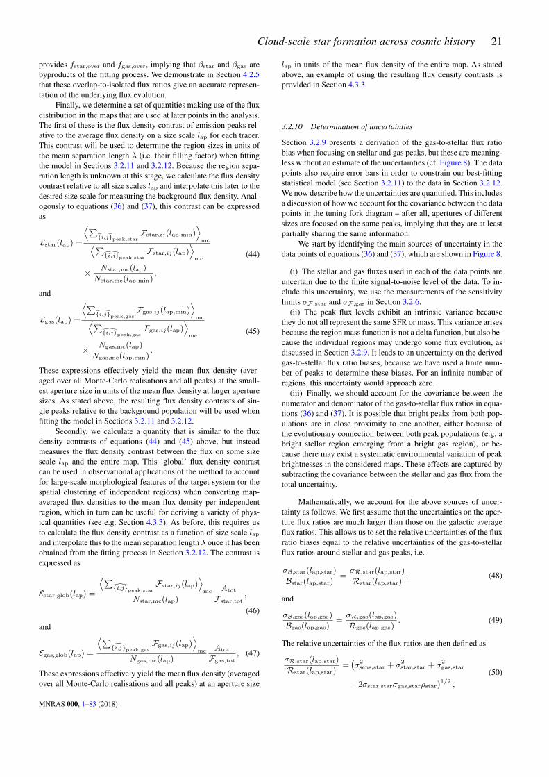
Cloud-scale star formation across cosmic history 21
provides fstar,over and fgas,over, implying that βstar and βgas arebyproducts of the fitting process. We demonstrate in Section 4.2.5that these overlap-to-isolated flux ratios give an accurate represen-tation of the underlying flux evolution.
Finally, we determine a set of quantities making use of the fluxdistribution in the maps that are used at later points in the analysis.The first of these is the flux density contrast of emission peaks rel-ative to the average flux density on a size scale lap for each tracer.This contrast will be used to determine the region sizes in units ofthe mean separation length λ (i.e. their filling factor) when fittingthe model in Sections 3.2.11 and 3.2.12. Because the region sepa-ration length is unknown at this stage, we calculate the flux densitycontrast relative to all size scales lap and interpolate this later to thedesired size scale for measuring the background flux density. Anal-ogously to equations (36) and (37), this contrast can be expressedas
Estar(lap) =
⟨∑{i,j}peak,star
Fstar,ij(lap,min)⟩
mc⟨∑{i,j}peak,star
Fstar,ij(lap)⟩
mc
× Nstar,mc(lap)
Nstar,mc(lap,min),
(44)
and
Egas(lap) =
⟨∑{i,j}peak,gas
Fgas,ij(lap,min)⟩
mc⟨∑{i,j}peak,gas
Fgas,ij(lap)⟩
mc
× Ngas,mc(lap)
Ngas,mc(lap,min).
(45)
These expressions effectively yield the mean flux density (aver-aged over all Monte-Carlo realisations and all peaks) at the small-est aperture size in units of the mean flux density at larger aperturesizes. As stated above, the resulting flux density contrasts of sin-gle peaks relative to the background population will be used whenfitting the model in Sections 3.2.11 and 3.2.12.
Secondly, we calculate a quantity that is similar to the fluxdensity contrasts of equations (44) and (45) above, but insteadmeasures the flux density contrast between the flux on some sizescale lap and the entire map. This ‘global’ flux density contrastcan be used in observational applications of the method to accountfor large-scale morphological features of the target system (or thespatial clustering of independent regions) when converting map-averaged flux densities to the mean flux density per independentregion, which in turn can be useful for deriving a variety of phys-ical quantities (see e.g. Section 4.3.3). As before, this requires usto calculate the flux density contrast as a function of size scale lap
and interpolate this to the mean separation length λ once it has beenobtained from the fitting process in Section 3.2.12. The contrast isexpressed as
Estar,glob(lap) =
⟨∑{i,j}peak,star
Fstar,ij(lap)⟩
mc
Nstar,mc(lap)
Atot
Fstar,tot,
(46)
and
Egas,glob(lap) =
⟨∑{i,j}peak,gas
Fgas,ij(lap)⟩
mc
Ngas,mc(lap)
Atot
Fgas,tot, (47)
These expressions effectively yield the mean flux density (averagedover all Monte-Carlo realisations and all peaks) at an aperture size
lap in units of the mean flux density of the entire map. As statedabove, an example of using the resulting flux density contrasts isprovided in Section 4.3.3.
3.2.10 Determination of uncertainties
Section 3.2.9 presents a derivation of the gas-to-stellar flux ratiobias when focusing on stellar and gas peaks, but these are meaning-less without an estimate of the uncertainties (cf. Figure 8). The datapoints also require error bars in order to constrain our best-fittingstatistical model (see Section 3.2.11) to the data in Section 3.2.12.We now describe how the uncertainties are quantified. This includesa discussion of how we account for the covariance between the datapoints in the tuning fork diagram – after all, apertures of differentsizes are focused on the same peaks, implying that they are at leastpartially sharing the same information.
We start by identifying the main sources of uncertainty in thedata points of equations (36) and (37), which are shown in Figure 8.
(i) The stellar and gas fluxes used in each of the data points areuncertain due to the finite signal-to-noise level of the data. To in-clude this uncertainty, we use the measurements of the sensitivitylimits σF,star and σF,gas in Section 3.2.6.
(ii) The peak flux levels exhibit an intrinsic variance becausethey do not all represent the same SFR or mass. This variance arisesbecause the region mass function is not a delta function, but also be-cause the individual regions may undergo some flux evolution, asdiscussed in Section 3.2.9. It leads to an uncertainty on the derivedgas-to-stellar flux ratio biases, because we have used a finite num-ber of peaks to determine these biases. For an infinite number ofregions, this uncertainty would approach zero.
(iii) Finally, we should account for the covariance between thenumerator and denominator of the gas-to-stellar flux ratios in equa-tions (36) and (37). It is possible that bright peaks from both pop-ulations are in close proximity to one another, either because ofthe evolutionary connection between both peak populations (e.g. abright stellar region emerging from a bright gas region), or be-cause there may exist a systematic environmental variation of peakbrightnesses in the considered maps. These effects are captured bysubtracting the covariance between the stellar and gas flux from thetotal uncertainty.
Mathematically, we account for the above sources of uncer-tainty as follows. We first assume that the uncertainties on the aper-ture flux ratios are much larger than those on the galactic averageflux ratios. This allows us to set the relative uncertainties of the fluxratio biases equal to the relative uncertainties of the gas-to-stellarflux ratios around stellar and gas peaks, i.e.
σB,star(lap,star)
Bstar(lap,star)=σR,star(lap,star)
Rstar(lap,star), (48)
and
σB,gas(lap,gas)
Bgas(lap,gas)=σR,gas(lap,gas)
Rgas(lap,gas). (49)
The relative uncertainties of the flux ratios are then defined as
σR,star(lap,star)
Rstar(lap,star)=(σ2
sens,star + σ2star,star + σ2
gas,star
−2σstar,starσgas,starρstar)1/2 ,
(50)
MNRAS 000, 1–83 (2018)

22 J. M. D. Kruijssen et al.
and
σR,gas(lap,gas)
Rgas(lap,gas)=(σ2
sens,gas + σ2star,gas + σ2
gas,gas
−2σstar,gasσgas,gasρgas)1/2 ,
(51)
respectively, where each of the uncertainties in parentheses repre-sent relative uncertainties and the negative terms represent the co-variance between the stellar and gas flux in the apertures. Each ofthese terms is defined below. As before, in the subscripts containinga comma, the word after the comma indicates the peak type that theapertures are focused on. The first term represents the uncertaintydue to the finite signal-to-noise level (or non-zero sensitivity), thesecond term represents the uncertainty on the stellar flux, the thirdterm represents the uncertainty on the gas flux, and the fourth termrepresents the covariance of the second and third terms. Finally,all terms have a dependence on the aperture size, but these depen-dences are omitted in the notation for brevity.
For the uncertainties due to the finite signal-to-noise level, wewrite
σ2sens,star =
[(σF,star
Fstar,star
)2
+
(σF,gas
Fgas,star
)2]
×(lap,star
lap,min
)−2
Nstar,mc,
(52)
and
σ2sens,gas =
[(σF,star
Fstar,gas
)2
+
(σF,gas
Fgas,gas
)2]
×(lap,gas
lap,min
)−2
Ngas,mc,
(53)
for apertures focused on stellar and gas peaks, respectively. As inequations (36) and (37), the double subscripts of the total fluxesfollow the order of indicating the flux type before the peak type.The relative uncertainty on the total flux due to noise in these ex-pressions follows normal statistics. Firstly, as mentioned in Sec-tions 3.2.3 and 3.2.5, the pixel flux values represent surface den-sities, implying that their uncertainty due to noise should decreasewith the square-root of the number of pixels in the apertureNpix,ap
and thus σ2 ∝ N−1pix,ap ∝ lap
−2. Secondly, the flux ratios ofequations (36) and (37) include the summation over all peaks inthe Monte-Carlo realisation, which means that the uncertainty σon the numerator and denominator should scale with N1/2
gas,mc andN
1/2star,mc, respectively. Both of these dependences are included in
equations (52) and (53). The division by the total flux in these equa-tions converts the absolute uncertainties to relative ones.
The uncertainties due to the intrinsic variance of the peak flux(e.g. by flux evolution or a region mass spectrum) are also straight-forward to define. Specifically, we take the standard deviation of theaperture fluxes for each of the four flux measurements (i.e. each ofthe two flux types around each of the two peak types) and convertthis to a relative uncertainty on the sum of all flux measurementsby writing
σ2star,star =
〈F2star,ij〉peak,star − 〈Fstar,ij〉2peak,star
F2star,star
Nstar,mc,
(54)
and
σ2gas,star =
〈F2gas,ij〉peak,star − 〈Fgas,ij〉2peak,star
F2gas,star
Nstar,mc, (55)
for apertures focused on stellar peaks (i.e. Rstar). Likewise, forapertures focused on gas peaks (i.e.Rgas) we define
σ2star,gas =
〈F2star,ij〉peak,gas − 〈Fstar,ij〉2peak,gas
F2star,gas
Ngas,mc, (56)
and
σ2gas,gas =
〈F2gas,ij〉peak,gas − 〈Fgas,ij〉2peak,gas
F2gas,gas
Ngas,mc. (57)
In these expressions, the numerator represents the variance (i.e. thestandard deviation squared) of the flux in a single aperture acrossthe population of stellar (subscript ‘peak,star’) or gas (subscript‘peak,gas’) peaks, the denominator represents the total flux that isused in the flux ratios of equations (36) and (37), and the factor Nat the end converts the variance of the flux in a single aperture tothat of the total flux.
Having defined all relative uncertainty terms that contribute toequations (50) and (51), we should subtract the relative covariancebetween the stellar and gas fluxes in the apertures, because Rstar
andRgas represent the ratios of these fluxes. For apertures focusedon stellar and gas peaks, the relative covariances are
cov(F)peak,star =〈Fstar,ijFgas,ij〉peak,star
− 〈Fstar,ij〉peak,star〈Fgas,ij〉peak,star,(58)
and
cov(F)peak,gas =〈Fstar,ijFgas,ij〉peak,gas
− 〈Fstar,ij〉peak,gas〈Fgas,ij〉peak,gas,(59)
respectively. These covariances define the correlation coefficientsbetween the stellar and gas fluxes in the apertures in equations (50)and (51) as
ρstar =cov(F)peak,star
σstar,starσgas,star, (60)
for apertures focused on stellar peaks and
ρgas =cov(F)peak,gas
σstar,gasσgas,gas, (61)
for apertures focused on gas peaks, respectively. Together, equa-tions (50)–(61) define the uncertainty on each individual data pointin equations (30) and (31). These are converted to uncertainties onthe logarithmic flux ratio bias by writing
σlog10 B =1
ln 10
σBB . (62)
The result of the presented uncertainty calculation is illustrated bythe error bars in Figure 10 for the example maps used throughoutthis section.
To determine the variances and covariances in equations (54)–(59), we calculate the flux averages across all peaks, instead ofevaluating the variance for each Monte-Carlo realisation of non-overlapping aperture samples and then taking the mean variance,or calculating the variance of the total flux across all Monte-Carlorealisations. As a result, equations (54)–(59) may seem lacking intwo regards.
(i) Firstly, these expressions do not account for the fact thatoverlapping apertures are omitted in each Monte-Carlo realisation.However, this is not necessarily incorrect, because pixels containedby multiple apertures are more likely to be drawn. Determining thevariance for each realisation would overestimate the variance due tothe range of environments covered by the maps. In the extreme ex-ample of large aperture sizes, the flux variance in each Monte-Carlo
MNRAS 000, 1–83 (2018)

Cloud-scale star formation across cosmic history 23
102 103 104
lap[pc]
10-1
100
101
B
gas peaks
stellar peaks
galactic average
Figure 10. Illustration of the uncertainties on the example tuning fork dia-gram of Figure 8. The error bars with hats indicate the uncertainty on eachindividual data point, without accounting for the covariance between thedata points. By contrast, the red (top) and blue (bottom) shaded areas be-hind each of the data points indicates the effective uncertainty range thataccounts for the correlation between the data points (see the text). These‘effective’ uncertainties are used when obtaining the best-fitting model inSection 3.2.12 and provide the correct point of reference when visually as-sessing the quality of a fit.
realisation may be based on a small number of peaks in widely dif-ferent parts of a galaxy, leading to a large aperture-to-aperture fluxvariance, even if the total flux may be similar in each Monte-Carlorealisation. Such a scenario arises naturally when the same environ-ments are included in each realisation. Overestimating the variancein this way would be highly undesirable.
(ii) Alternatively, one could take the variance of the total fluxesacross all Monte-Carlo realisations. However, this would underesti-mate the variance – if none of the peaks is overlapping, then the to-tal flux variance between the Monte-Carlo realisations will be zero,because all peaks are included in each realisation. This would givethe erroneous impression that the variance is constrained to infiniteprecision, which gravely underestimates the variance at small aper-ture sizes. However, the non-zero variance only reflects the pointthat the total number of peaks in the maps is finite. This finite peaksample itself should be seen as one possible realisation of an under-lying physical distribution of peak fluxes, which implies a non-zerovariance of the total flux even if all peaks are included.
We find that taking the variance of all aperture fluxes, irrespec-tive of whether an aperture is included or not, provides an accuratemiddle ground between the above two extremes. It accounts forthe fact that pixels contained by multiple apertures are more likelyto be drawn in each Monte-Carlo realisation, while also properlyaccounting for the fact that the peak population itself representsone possible realisation of the underlying physical flux distribu-tion function. The uncertainties due to the intrinsic variance of thepeak flux are therefore defined by averaging over all peaks in equa-tions (54)–(59).
The error bars derived above are corrected for the correlationbetween the numerator and denominator in the gas-to-stellar flux
ratios of equations (36) and (37), but they do not account for thefact that the data points in the tuning fork diagram are not inde-pendent. This dependence arises because the apertures of differentsizes are focused on the same peaks, implying that some fractionof the flux contained by apertures of a certain size is also presentin apertures of other sizes. We correct for this dependence betweenthe data points during the fitting process in Section 3.2.12 by cal-culating their normalised ‘independence fraction’, which representsthe fraction of the flux in a data point that is independent from theflux in all other data points, and using this quantity to weigh thecontribution of each data point to the goodness-of-fit statistic. Thesum of these independence fractions corresponds to the total num-ber of independent data points that the model from Section 3.2.11is fitted to. The net effect of accounting for the correlation betweendata points is to decrease the number of degrees of freedom, lead-ing to a larger difference between the model and the data. This isequivalent to decreasing the error bars on the data points, which isillustrated by the red and blue shaded areas behind each data pointin Figure 10. These shaded areas represent ‘effective’ uncertaintiesthat should be used for visually evaluating the quality of a fit. In thetext below, we derive these effective uncertainties.
First, we determine for each aperture size which fraction ofthe flux is independent from the flux in the other apertures. Forthe stellar and gas flux around stellar peaks, we define the fractionof the flux at an aperture size lap(j) that is also contained by anaperture of (smaller) size lap(i), with {i, j ∈ N|i 6 j}, to be
Nstar,star =Fstar,star[lap(i)]
Fstar,star[lap(j)]
Nstar,mc[lap(j)]
Nstar,mc[lap(i)]
[lap(i)
lap(j)
]2
, (63)
and
Ngas,star =Fgas,star[lap(i)]
Fgas,star[lap(j)]
Nstar,mc[lap(j)]
Nstar,mc[lap(i)]
[lap(i)
lap(j)
]2
, (64)
respectively. Similarly, for the stellar and gas flux around gas peaks,we define the fraction of the flux at an aperture size lap(j) that isalso contained by an aperture of (smaller) size lap(i), with {i, j ∈N|i 6 j}, to be
Nstar,gas =Fstar,gas[lap(i)]
Fstar,gas[lap(j)]
Ngas,mc[lap(j)]
Ngas,mc[lap(i)]
[lap(i)
lap(j)
]2
, (65)
and
Ngas,gas =Fgas,gas[lap(i)]
Fgas,gas[lap(j)]
Ngas,mc[lap(j)]
Ngas,mc[lap(i)]
[lap(i)
lap(j)
]2
, (66)
respectively. As before, we have followed the convention that thefirst word of a subscript indicates the type of flux and the secondword indicates the peak type that the apertures are focused on. Wesymmetrise these four arrays by setting
N(j, i|i 6 j) = N(i, j|i 6 j), (67)
for each of them. As a result, array elements with i > j indicate thefraction of the flux at an aperture size lap(i) that is also containedby an aperture of (smaller) size lap(j). For all four arrays, settingi = j gives N = 1, indicating the trivial result that an aperturecontains all of the flux within that aperture.
Equations (63)–(66) define the fraction of the flux in a largeraperture that is ‘reused’ from a smaller aperture, for each aperturesize pair. The above definitions imply that by performing a summa-tion over one of the dimensions in these ‘reuse’ fraction arrays, oneobtains the non-integer number of data points that are constitutedby the flux contained within an aperture of size lap(i), i.e.
Ndata(i) =∑j
N(i, j), (68)
MNRAS 000, 1–83 (2018)

24 J. M. D. Kruijssen et al.
which returns a number 1 < Ndata[lap(i)] 6 Nap. We then definethe ‘independence fraction’ of the flux at an aperture size lap(i) asthe inverse of this number
fdata(i) =1
Ndata=
1∑j N(i, j)
, (69)
which takes values of 0 < fdata < 1. Because the flux ratio biasesof equations (30) and (31) that are shown in Figure 10 representflux ratios, we define the independence fraction of each data pointas the mean of the fluxes in the numerator and the denominator,resulting in
fdata,star(i) =1
2∑j Nstar,star(i, j)
+1
2∑j Ngas,star(i, j)
, (70)
and
fdata,gas(i) =1
2∑j Nstar,gas(i, j)
+1
2∑j Ngas,gas(i, j)
, (71)
respectively. The total number of independent data points in eachof the arms of the tuning fork diagram then follows as
Nindep,star =∑i
fdata,star(i), (72)
and
Nindep,gas =∑i
fdata,gas(i), (73)
for the bottom arm and the top arm of the diagram, focusing onstellar peaks and gas peaks, respectively. The total number of inde-pendent data points is therefore smaller than twice the number ofaperture sizes, i.e.
Nindep = Nindep,star +Nindep,gas < 2Nap. (74)
As stated above, the correlation between data points is ac-counted for during the fitting process of Section 3.2.12 by weigh-ing the contribution of each data point to the goodness-of-fit statis-tic by its normalised independence fraction. We also decrease thenumber of degrees of freedom by using the total number of inde-pendent data points Nindep rather than the total number of datapoints 2Nap. The net effect of these changes is equivalent to de-creasing the uncertainties σB to becoming ‘effective uncertainties’σ′B. The weights and degrees of freedom are discussed in detail inSection 3.2.12, but here we provide these effective uncertainties.Relative to the error bars defined in equations (48) and (49), weobtain correction factors of
σ′log10 Bstar(i)
σlog10 Bstar(i)=
√Nindep
2fdata,star(i)Nap
Nindep −Nfit
2Nap −Nfit, (75)
and
σ′log10 Bgas(i)
σlog10 Bgas(i)=
√Nindep
2fdata,gas(i)Nap
Nindep −Nfit
2Nap −Nfit, (76)
for the gas-to-stellar flux ratio bias when focusing on stellar peaksand gas peaks, respectively. The square-roots in these expressionscontain two ratios. The first term reflects the inverse of the weightthat is assigned to the data points when evaluating the goodness-of-fit statistic. The second term represents the decrease of the numberof degrees of freedom by only counting the effective number ofindependent data points, where Nfit refers to the number of freeparameters (this is Nfit = 3 for the problem considered here, seeSection 3.2.12 for details). The above two expressions provide theeffective uncertainties shown by the shaded areas in Figure 10.
3.2.11 Model for interpreting the gas-to-stellar flux ratio bias
We now turn to the derivation of the theoretical model for the gas-to-stellar flux ratio bias that will be fitted to the observed tuningfork diagram of Figure 10 in Section 3.2.12 below. The presenta-tion in the original KL14 principle paper already included a the-oretical model for the flux ratio bias (see their Appendix C), butthe model presented here eliminates an important assumption ofthe previous version. Previously, the model assumed that all inde-pendent regions in the map resemble point sources, implying thatthe surface densities approach infinity in the limit of lap ↓ 0. Thisthen leads to a flux ratio bias that diverges at small aperture sizes iftover = 0 (see Figure 4 of KL14). In the present paper, we describethe regions by spatial profiles with finite central densities, which isobviously appropriate for real-Universe regions. This implies thata non-diverging flux ratio bias at small aperture sizes does not nec-essarily require tover > 0. This change is critical for the accu-racy of observational applications of the method. After presentingthe derivation of the new model, we will briefly discuss the effecton the predicted flux ratio bias of changing the model parameters.These include the to-be-fitted, free parameters tgas, tover, and λ, aswell as input parameters of the method (tstar and peak prof) andparameters that have been extracted from the maps in the previoussections (βstar, βgas, Estar, and Egas).
In deriving the new model, we will start by taking the resultfrom KL14 and then modify it to introduce the peak surface densityprofiles. In the original model, the gas-to-stellar flux ratio bias isobtained by counting regions within the aperture. The flux from thepeak type (i.e. stars or gas) that the apertures are focused on is con-stituted by the sum of the central peak and the statistically expectedbackground flux from other peaks. By contrast, the flux from theother tracer is constituted by the sum of the statistically expectedbackground flux from other peaks and the central peak if it spendsany time in the overlap phase. This latter contribution depends onthe time-scales involved – for stellar peaks, the probability thatthe central peak also contains gas flux is fstar,over = tover/tstar,whereas the probability that gas peaks also contain stellar flux isfgas,over = tover/tgas. This contribution should also be correctedfor any evolution of the peak flux, which may result in fluxes dur-ing the overlap phase that differ from those in the isolated phase (ascaptured by the parameters βstar and βgas, see Section 3.2.9).
The expressions for the gas-to-stellar flux ratio bias are de-rived in Appendix C of KL14 and we refer the interested readerto that earlier work for the details of the derivation. The gas-to-stellar flux ratio bias when focusing apertures on stellar peaks (cor-responding to the bottom branch in the tuning fork diagram) is
BKL14star =
[1 + β−1
gas
(tgas
tover− 1)]−1
+ tstarτ
(lap
λ
)2
1 + tstarτ
(lap
λ
)2 . (77)
When focusing on gas peaks (top branch in the tuning fork dia-gram), the bias is given by
BKL14gas =
1 +tgasτ
(lap
λ
)2
[1 + β−1
star
(tstartover
− 1)]−1
+tgasτ
(lap
λ
)2 , (78)
Each of the variables in these expressions have already been in-troduced, but for clarity we briefly repeat them. The time-scaleτ = tstar+tgas−tover is the total duration of the evolutionary time-line in Figure 1, tstar is the duration of the stellar phase, tgas is theduration of the gas phase, tover is the duration of the overlap phase,
MNRAS 000, 1–83 (2018)

Cloud-scale star formation across cosmic history 25
λ is the mean separation length between independent regions, lap
is the aperture size, and βstar and βgas represent the flux ratios be-tween the overlap phase and the isolated phase of stellar peaks andgas peaks, respectively. In both of the above two expressions, theterms containing the square of the aperture size represent the back-ground flux from other peaks, the ‘1’ represents the peak that theaperture is focused on, and the terms containing tover represent thecontribution from that peak to the other tracer if it resides in theoverlap phase. A change relative to KL14 that is not immediatelyvisible in these expressions is that βstar and βgas are now treated asfunctions of fstar,over = tover/tstar and fgas,over = tover/tgas. Inthe exploration of the model behaviour below, we will treat theseas independent parameters, but when fitting the model to the ob-served tuning fork diagram in Section 3.2.12, βstar and βgas arenot independent variables.
As a consequence of fully counting the peak that is being fo-cused on (as well as fully counting any contribution from this peakto the other tracer if it resides in the overlap phase), irrespectiveof the aperture size, these formulations implicitly assume that thepeak profiles are delta functions, i.e. that their radii are infinitesi-mally small. As a result, gas-to-stellar flux ratios of equations (77)and (78) diverge when tover ↓ 0. This can be seen directly by takingthe limits of lap ↓ 0, which yields
limlap↓0
BKL14star =
[1 + β−1
gas
(tgas
tover− 1
)]−1
, (79)
and
limlap↓0
BKL14gas = 1 + β−1
star
(tstar
tover− 1
). (80)
If tover ↓ 0, these expressions approach zero and infinity, respec-tively. This result led us to conclude in KL14 that the flattening ofthe tuning fork diagram at small aperture sizes provides a way ofmeasuring tover. While this is still true, we pointed out above thatthe real-Universe situation is more complex, because the flatteningof the tuning fork diagram is not unique to a non-zero duration ofthe overlap phase. Real molecular clouds or star-forming regionsare not infinitesimally small and their finite central densities pro-vide another way of avoiding divergence.
We account for the peak surface density profiles by introduc-ing an extra factor in equations (77) and (78) that takes values be-tween 0 and 1 and represents the fraction of the flux from the centralpeak that is contained within the aperture. This factor is only addedto the terms that represent the stellar and gas flux contribution fromthe central peak. For the randomly-distributed, background popula-tion of spatially-extended peaks in and around the aperture, the fluxcontributions from peaks with centres outside of the aperture can-cel on geometric grounds with the flux loss from peaks with centreswithin the aperture. As a result, the background flux in the apertureis exclusively set by the number surface density of the peaks and isinsensitive to their individual surface density profiles.16 This allowsus to formulate the updated version of the KL14 principle model as
Bmodstar =
fgas
[1 + β−1
gas
(tgas
tover− 1)]−1
+ tstarτ
(lap
λ
)2
fstar + tstarτ
(lap
λ
)2 , (81)
16 We thank Sophie Kruijssen for pointing out this logic, which has led toan important simplification of the model.
and
Bmodgas =
fgas +tgasτ
(lap
λ
)2
fstar
[1 + β−1
star
(tstartover
− 1)]−1
+tgasτ
(lap
λ
)2 , (82)
where fstar and fgas represent the fraction of the central peak fluxthat is contained by the aperture, with the subscripts referring tostellar peaks and gas peaks respectively. These expressions are usedthroughout the rest of this paper.
Equations (81) and (82) do not yet show how fstar and fgas
depend on the aperture size. We will specify this below for a smallnumber of useful peak surface density profiles. However, in defin-ing the above expressions, we have already made an important as-sumption. The enclosed flux fraction of the central peak is assumedto differ between both tracers, because a factor of fgas appears inthe numerator and a factor of fstar appears in the denominator ofequations (81) and (82). This means that we allow the flux fromboth tracers to follow different profiles, which provides some use-ful flexibility and is consistent with observations (e.g. Walker et al.2015, 2016). However, we also assume that there is no difference inprofile shape between peaks of a given tracer that reside in the iso-lated and overlap phases, because the same factors of fstar and fgas
are used in equations (81) and (82). This may introduce a minor in-consistency in cases where there is considerable time-evolution ofthe peak size. In practical applications, however, this typically hap-pens on size scales below the resolution limit, because we convolvethe maps to a common resolution lap,min (see Section 3.2.3). It isdemonstrated in Section 4 that the method yields accurate measure-ments of tover, to such an extent that any effect of this inconsistencymust fall within acceptable limits. Indeed, we have verified thatthe results do not change (i.e. they stay well within the obtaineduncertainties) when dividing the peak sample in peaks residing inthe isolated and overlap phases before determining the flux densityprofiles. It is therefore undesirable to add another layer of com-plexity that could address this, in particular because we have no apriori constraints on how the peak profiles change with evolution-ary stage.
We consider three different types of surface density profiles tomodel the peak emission, all of which are available in HEISEN-BERG. However, only the third of these profiles will be usedthroughout the rest of the paper, for reasons outlined below. Eachof these profiles is normalised to have a total flux fraction of unity(i.e. limlap→∞
f(lap) = 1), so that at infinitely large aperture sizesthe entire peak resides within the aperture. The profiles are as fol-lows.
(i) A two-dimensional delta function that is centred on the peakposition, resulting in an enclosed flux fraction as a function of aper-ture size that is given by
fδ(lap) = 1. (83)
This corresponds to the case derived in KL14, where we assumedthat the peaks correspond to points.
(ii) A two-dimensional, constant surface density disc that is cen-tred on the peak position, resulting in an enclosed flux fraction as afunction of aperture size that is given by
fdisc(lap) =
{(lap/2rpeak)2 if lap < 2rpeak
1 if lap > 2rpeak.(84)
In this expression, rpeak represents the radius of the constant sur-face density disc. We discuss below how this radius is obtainedfrom the galaxy maps.
MNRAS 000, 1–83 (2018)

26 J. M. D. Kruijssen et al.
(iii) A two-dimensional Gaussian centred on the peak position,resulting in an enclosed flux fraction as a function of aperture sizethat is given by
fGauss(lap) = 1− exp
[−1
2
(lap
2rpeak
)2]. (85)
In this expression, rpeak represents the dispersion of the two-dimensional Gaussian. We discuss below how this scale radius isobtained from the galaxy maps.
The second and third of these profiles require the characteris-tic peak radius rpeak to be known. However, it is straightforwardto obtain this from the galaxy maps once a peak profile has beenassumed to approximate the flux density profiles of the peaks inthe maps. In Section 3.2.9, we measured the flux density contrastof emission peaks to the average flux density on a size scale lap inequations (44) and (45). This flux ratio contrast can be related tothe ratio between the central surface density of peaks and the back-ground surface density of the peak population. In turn, this allowsus to express the peak radius rpeak in units of the region separa-tion length λ. For the stellar and gas flux, the background numberdensities of independent regions are
Σback,star =tstar
τ
(πλ2
4
)−1
, (86)
and
Σback,gas =tgas
τ
(πλ2
4
)−1
, (87)
respectively. In these expressions, the term in parentheses uses themean separation length between independent regions to representthe area per region, whereas the multiplications by tstar/τ andtgas/τ reduce the resulting total number densities to only refer tothe number densities of stellar peaks and gas peaks, respectively.
For a constant surface density disc normalised to unity, thecentral surface density is
Σdisc =1
πr2peak
, (88)
whereas for a two-dimensional Gaussian normalised to unity, thecentral surface density is
ΣGauss =1
2πr2peak
. (89)
With the expected background and central flux densities in hand,it is now possible to relate these to the flux density contrasts Estar
and Egas as a function of aperture size obtained in equations (44)and (45) above (see Section 3.2.9). This will provide the peak ra-dius rpeak in units of the region separation length λ.
Because Estar and Egas represent flux density contrasts mea-sured relative to a variable aperture size, there is some freedom inchoosing the size scale on which the flux density contrast is evalu-ated. We find that it is desirable to define Estar and Egas on a sizescale λ, because on larger scales the considered maps may containvoids or other morphological features that change the surface num-ber density of regions from the density in the direct vicinity of thepeaks implied by the best-fitting λ. By setting the size scale to λ,the background surface number density of neighbouring peaks bestcorresponds to the measured region separation length. In practice,this means that when fitting the observed tuning fork diagram inSection 3.2.12 below, Estar and Egas are both varied with λ and areconstrained as a byproduct of the fitting process.
On a size scale λ, the measured flux ratio contrasts definedin equations (44) and (45) can be expressed in terms of the abovecentral and background number densities as
Estar ≡ Estar(λ) =Σpeak + Σback,star
(πλ2/4)−1 + Σback,star, (90)
and
Egas ≡ Egas(λ) =Σpeak + Σback,gas
(πλ2/4)−1 + Σback,gas, (91)
where Σpeak refers to Σdisc or ΣGauss depending on the adoptedprofile. In these two expressions, the numerator represents the fluxdensity on a size scale lap,min, consisting of the central surface den-sity of the peak (first term) and the background population (secondterm), and the denominator represents the flux density on a sizescale λ, consisting of the entire central peak (first term) and thebackground population (second term).
Rearranging the above expressions allows the characteristicpeak radii to be expressed in terms of quantities that are either mea-sured directly from the maps (Estar and Egas), or represent free pa-rameters during the fitting process in Section 3.2.12 (τ , tgas, andλ). If we represent the peaks with constant surface density discs,we obtain for the radii of stellar peaks
rstar =λ
2
√τ/tstar
Estar(1 + τ/tstar)− 1, (92)
and for the radii of gas peaks
rgas =λ
2
√τ/tgas
Egas(1 + τ/tgas)− 1. (93)
Likewise, if we represent the peaks with two-dimensional Gaussianprofiles, we obtain for the radii of stellar peaks
rstar =λ
2
√τ/tstar
2Estar(1 + τ/tstar)− 2, (94)
and for the radii of gas peaks
rgas =λ
2
√τ/tgas
2Egas(1 + τ/tgas)− 2. (95)
Equations (92)–(95) are substituted into the enclosed flux fractionsas a function of aperture size from equations (84) and (85). Sub-stitution of the result into equations (81) and (82) yields the pre-dicted gas-to-stellar flux ratio bias when focusing apertures on stel-lar peaks and gas peaks, respectively, in terms of measurable quan-tities and free parameters of the fitting process in Section 3.2.12.
When applying the method to real-Universe observations or tothe simulated galaxy maps in Section 4, the Gaussian peak surfacedensity profile fGauss is generally the best choice to make. Aboveall, it is versatile – in the limit of a very large flux ratio excess E , thepeak radii approach zero and hence the possible range of profilesincludes a reasonable approximation of the delta function profilefδ to represent point particles. This feature is also shared by theconstant surface density disc profile fdisc, but the Gaussian profileis more suitable for two other reasons. Firstly, the regridding of themaps in Section 3.2.3 is accompanied by a convolution of the mapswith a Gaussian PSF to a common resolution. This means that un-resolved peaks have Gaussian profiles by definition and resolvedpeaks at least have a Gaussian component. Secondly, real-Universemolecular clouds and star-forming regions generally follow cen-trally concentrated morphologies, rather than having constant sur-face densities (e.g. Walker et al. 2015, 2016). Gaussian profiles
MNRAS 000, 1–83 (2018)
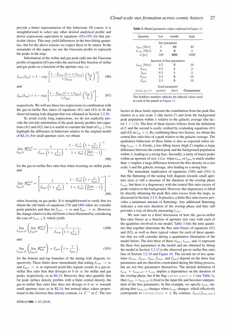
Cloud-scale star formation across cosmic history 27
provide a better representation of this behaviour. Of course, it isstraightforward to select any other desired analytical profile andderive expressions equivalent to equations (92)–(95) for that par-ticular choice. This may yield differences in the best-fitting quanti-ties, but for the above reasons we expect these to be minor. In theremainder of this paper, we use the Gaussian profile to representthe peaks in the map.
Substitution of the stellar and gas peak radii into the Gaussianprofile of equation (85) provides the enclosed flux fraction of stellarand gas peaks as a function of the aperture size, i.e.
fstar(lap) = 1− exp
[1− Estar (1 + τ/tstar)
τ/tstar
(lap
λ
)2], (96)
and
fgas(lap) = 1− exp
[1− Egas (1 + τ/tgas)
τ/tgas
(lap
λ
)2], (97)
respectively. We will use these two expressions in combination withthe gas-to-stellar flux ratios of equations (81) and (82) to fit theobserved tuning fork diagram that was obtained in Section 3.2.10.
To avoid overly long expressions, we do not explicitly pro-vide the (trivial) substitution of the peak density profiles into equa-tions (81) and (82), but it is useful to consider the limit of lap ↓ 0 tohighlight the difference in behaviour relative to the original modelof KL14. For small aperture sizes, we obtain
limlap↓0
Bmodstar =
1
Estar
(1 + τ
tstar
) +1− E−1
star
(1 + τ
tstar
)−1
1 + β−1gas
(tgas
tover− 1) ,
(98)
for the gas-to-stellar flux ratio bias when focusing on stellar peaksand
limlap↓0
Bmodgas =
1
Egas
(1 + τ
tgas
) +1− E−1
gas
(1 + τ
tgas
)−1
1 + β−1star
(tstartover
− 1)−1
,
(99)
when focusing on gas peaks. It is straightforward to verify that weobtain the old limits of equations (79) and (80) when we considerpoint particles and thus let Estar → ∞ and Egas → ∞. However,the change relative to the old limits is best illustrated by consideringthe case of tover ↓ 0, which yields
limtover↓0
(limlap↓0
Bmodstar
)=
1
Estar
(1 + τ
tstar
) , (100)
and
limtover↓0
(limlap↓0
Bmodgas
)= Egas
(1 +
τ
tgas
), (101)
for the bottom and top branches of the tuning fork diagram, re-spectively. These limits show immediately that setting Estar → ∞and Egas → ∞ to represent point-like regions results in a gas-to-stellar flux ratio bias that diverges to 0 or ∞ for stellar and gaspeaks, respectively, as in KL14. However, they also quantify thatfor peak surface density profiles with a finite central density, thegas-to-stellar flux ratio bias does not diverge to 0 or ∞ towardssmall aperture sizes as in KL14, but instead takes values propor-tional to the (inverse) flux density contrast, i.e. E−1 or E . The two
Table 3. Model parameter values explored in Figure 11
Quantity low middle high
free parametertgas [Myr] 5 10 20
tover [Myr] 0 2 4λ [pc] 100 300 1000
function of free parameterststar [Myr] 2.5 5 10
βstar 0.5 1 2
βgas 0.5 1 2Estar 2.5 5 10
Egas 2.5 5 10
fixed parameterpeak prof points discs Gaussians
The boldface numbers indicate the fiducial values usedin each of the panels in Figure 11.
factors in these limits represent the contribution from the peak fluxrelative to a size scale λ (the factor E) and from the backgroundpeak population within λ relative to the galactic average (the fac-tor 1 + τ/t). The first of these factors follows from the definitionof E and the second is easily verified by evaluating equations (81)and (82) at lap = λ. By combining these two factors, we obtain thecentral flux ratio bias of a peak relative to the galactic average. Thequalitative behaviour of these limits is also as expected when set-ting tover = 0. Firstly, a low filling factor (high E) implies a largedifference between the central peak and the background populationwithin λ, leading to a strong bias. Secondly, a rarity of tracer peakswithin an aperture of size λ (i.e. when tstar or tgas is much smallerthan τ ) implies a large difference between the flux density on a sizescale λ and the galactic average, also leading to a strong bias.
The immediate implication of equations (100) and (101) isthat the flattening of the tuning fork diagram towards small aper-ture sizes is still a measure of the duration of the overlap phasetover, but there is a degeneracy with the central flux ratio excess ofpeaks relative to the background. However, this degeneracy is liftedby directly obtaining the peak flux ratio excess from the maps, asdiscussed in Section 3.2.9. In practice, a finite flux ratio excess pro-vides a minimum amount of flattening. Any additional flatteningindicates a non-zero duration of the overlap phase and thus stillprovides a way of directly measuring tover.
We now turn to a brief discussion of how the gas-to-stellarflux ratio biases as a function of aperture size vary with each ofthe quantities involved in our model. Table 3 lists the nine quanti-ties that together determine the flux ratio biases of equations (81)and (82), as well as three typical values for each of these quanti-ties that we will consider during a quantitative illustration of themodel below. The first three of these (tgas, tover, and λ) representthe three free parameters in the model and are obtained by fittingthe model in Section 3.2.12 to the observed gas-to-stellar flux ratiobias of Section 3.2.10 and Figure 10. The second set of five quan-tities (tstar, βstar, βgas, Estar, and Egas) depend on the three freeparameters and are therefore constrained during the fitting process,but are not free parameters themselves. The default definition oftstar = tstar,ref + tover implies a dependence on the duration ofthe overlap phase, but if the flag tstar incl = 1 (see Table 1),then tstar = tstar,ref is fixed in the input file and becomes indepen-dent of the free parameters. In this example, we specify tstar, im-plying that tstar,ref changes when tover changes, which effectivelycorresponds to tstar incl = 1. By contrast, βstar(fstar,over)
MNRAS 000, 1–83 (2018)

28 J. M. D. Kruijssen et al.
and βgas(fgas,over) always depend on the free parameters, becausethey depend on the ratios tover/tstar and tover/tgas, respectively,as described in Section 3.2.9 and illustrated in Figure 9. Likewise,Estar(λ) and Egas(λ) both depend on the mean separation length λ(see Section 3.2.9). While these five quantities will vary as a func-tion of tgas, tover, and λ in practical applications of the method,we consider them as free parameters in the example given here,with the goal of isolating their effects. The final quantity in Table 3(peak prof) represents a fixed parameter that is set in the inputparameter file. This quantity therefore influences the shape of themodelled tuning fork diagram, but does not vary during the fittingprocess of Section 3.2.12.
Figure 11 systematically shows how each of the nine quan-tities from Table 3 affect the shape of the modelled gas-to-stellarflux ratio bias as a function of the aperture size. The main resultof the parameter study in the figure is that each of the nine quan-tities in general, but especially the three free parameter in particu-lar, have a unique effect on the shapes of the curves. This meansthat the gas-to-stellar flux ratio bias is a non-degenerate functionof these quantities, allowing the free parameters to be measuredby fitting the model to observed tuning fork diagrams. The basicbehaviour is the same as in the schematic of Figure 2. When fo-cusing apertures on stellar (gas) peaks, the gas-to-stellar flux ratiois smaller (larger) than the galactic average. This gas-to-stellar fluxratio bias increases towards decreasing aperture sizes, because thecentral peak contributes a larger fraction to the total flux ratio inthe aperture when a smaller population of other peaks is included.However, the bias does not grow indefinitely towards small aper-tures. As discussed in the above derivation, this arises for two rea-sons. Firstly, if the stellar and gas phases overlap in time, then thereis a non-zero probability that a peak resides in the overlap phase andemission from both tracers is present. This limits the gas-to-stellarflux ratio bias when preferentially selecting one type of tracer. Sec-ondly, peaks have finite central surface densities, implying that forthe smallest aperture sizes, the gas-to-stellar flux ratio bias reflectsthe overdensity of the peaks relative to the background populationof other peaks, as demonstrated in equations (100) and (101).
Starting with the top row of Figure 11, we see in panel (a) thatincreasing tgas decreases the bottom branch of the tuning fork dia-gram, i.e. it leads to a larger gas-to-stellar flux deficit when focusingon stellar peaks. This happens because for larger tgas, the overlapphase (which sets the bias at small aperture sizes) takes up a smallerfraction of the total duration of the gas phase, implying that stellarpeaks residing in the overlap phase contribute a smaller fraction ofthe galactic gas flux. Due to the relatively smaller ‘damping’ effectof the gas flux from stellar peaks in the overlap phase the bottombranch flattens less if tgas is larger. By contrast, changing the du-ration of the gas phase does not affect the relative contribution ofthe stellar flux from gas peaks in the overlap phase to the galac-tic stellar flux, because this is mainly set by the ratio tover/tstar
in equation (82). The flattening of the top branch is therefore onlyweakly affected by changing tgas. There is a small decrease of theaperture size below which the gas-to-stellar flux ratio bias sets inwhen increasing tgas. This is easily understood – gas peaks becomemore common as tgas increases, causing their number density to in-crease too. Therefore, a smaller aperture size is required to isolatethe contribution from the gas peak that the aperture is focused on.
The second free parameter is the duration of the overlap phasetover. Panel (b) shows that the effect of increasing tover is that theprobability that the central peak in the aperture also contains emis-sion from the other tracer increases. This limits the gas-to-stellarflux ratio bias relative to the galactic average that can be achieved
at the smallest aperture sizes and therefore leads to a stronger flat-tening of the model tuning fork diagram towards larger tover. Thefigure again illustrates the key difference relative to KL14, namelythat the branches of the tuning fork do not diverge towards smallaperture sizes when tover = 0, due to the finite central surfacedensities of the two-dimensional Gaussians used here. Most im-portantly, the behaviour due to tover fundamentally differs from theinfluence of tgas on the gas-to-stellar flux ratio bias. While the latteraffects the vertical position of one of the branches and only weaklyaffects the horizontal position of the other branch, the former sym-metrically sets the vertical positions of both branches.
The third free parameter is the mean separation length be-tween independent regions λ. Its effect on the shape of the tun-ing fork is easy to understand. Panel (c) shows that increasing theseparation length means that the entire model tuning fork diagramshifts to larger aperture sizes, because recovering the galactic aver-age by encompassing a sufficient number of regions in the aperturerequires a larger aperture area. Crucially, the effect of the separa-tion length is orthogonal to that of tgas and tover, as it controls theoverall horizontal position of the diagram.
We briefly summarise the effects of the three free parametersduring the fitting process of our model.
(i) The ratio between tgas and tstar sets the vertical asymmetryof the model tuning fork diagram.
(ii) The duration of the overlap phase tover sets the flattening ofthe tuning fork towards small aperture sizes.
(iii) The mean separation length of independent regions λ setsthe horizontal position of the model tuning fork.
The quantities in panels (d)–(h) of Figure 11 depend on thefree parameters tgas, tover, and λ from the first row. When chang-ing either of these free parameters during the fitting process, theireffect on the tuning fork diagram will therefore be accompaniedby the change seen in one or more of panels (d)–(h). The durationof the stellar phase tstar = tstar,ref + tover is varied in panel (d)and mirrors the behaviour of changing tgas in panel (a). In addi-tion, because tstar increases with tover, the increased flattening ofthe curves towards large values of tover is accompanied by a slightincrease of the gas-to-stellar flux ratio excess in the top branch andan even smaller inwards shift of the bottom branch. We note thatthe effect of changing tstar on the bottom branch in panel (d) islarger than that of changing tgas on the top branch in panel (a).This is caused by the fact that we have set tgas > tstar in thisexample. As a result of this dissimilarity, the flattening of the topbranch in panel (a) is affected more strongly by the high probabilitythat young stellar peaks reside in the overlap phase and are there-fore included when focusing on gas peaks, which does not dependon tgas, whereas the flattening of the bottom branch in panel (d)is affected more strongly by the flux density contrast of the centralpeak relative to its immediate surroundings, which does depend ontstar. This difference can be quantitatively verified by inspection ofequations (98) and (99).
Panel (e) shows the influence of changing the overlap-to-isolated flux ratio of stellar emission. Unsurprisingly, this only af-fects the top branch, where the incidence of stellar emission fromgas peaks in the overlap phase flattens the tuning fork. This flat-tening becomes stronger if the stellar emission from peaks in theoverlap phase is brighter than from those in the isolated phase(i.e. βstar > 1) and weakens if the stellar emission from peaks inthe overlap phase is fainter (i.e. βgas < 1). The same behaviour isseen for the bottom branch in Panel (f), which shows the influenceof changing the overlap-to-isolated flux ratio of gas emission. Be-
MNRAS 000, 1–83 (2018)

Cloud-scale star formation across cosmic history 29
10-1
100
101gas peaks
stellar peaks
(a)
free parameter
tgas
5.010.020.0
(b)
free parameter
tover
0.01.02.0
(c)
free parameter
λ100300
1000
10-1
100
101
B
(d)
function of free parameters
tstar
2.55.0
10.0
(e)
function of free parameters
βstar
0.51.02.0
(f)
function of free parameters
βgas
0.51.02.0
102 103
10-1
100
101(g)
function of free parameters
Estar
2.55.0
10.0
102 103
lap[pc]
(h)
function of free parameters
Egas
2.55.0
10.0
102 103
(i)
fixed parameter
peak_profpoints
discsGaussians
Figure 11. Predicted gas-to-stellar flux ratio bias as a function of the aperture size when focusing apertures on stellar peaks (bottom branches) or gas peaks(top branches), as indicated by the grey labels in panel (a). In each panel, the effect of varying one model quantity is shown relative to the fiducial parameterset (see Table 3). The values in the top right corner of each panel show the values used, with the fiducial choice shown in black. In the bottom right cornerof each panel, we list the nature of each quantity. The quantities varied in panels (a)–(c) are all free parameters in the model, meaning that they are fittedfor in Section 3.2.12. The quantities varied in panels (d)–(h) are all a function of the three free parameters in the top row, implying that while they will beconstrained during the fitting process, they are not free parameters as such. Finally, the quantity peak prof that is varied in panel (i) is fixed prior to startingthe fitting process. The figure shows that each of the free parameters has a unique effect on the shapes of the curves, implying that they are non-degenerate andcan therefore be measured by fitting our model to observed tuning fork diagrams.
cause βstar and βgas depend on tover/tstar and tover/tgas, respec-tively, a change of the model tuning fork diagram due to any of thethree time-scales can be accompanied by a change as seen in pan-els (e) or (f). This could hamper the accuracy of the method if thecorresponding changes in βstar and βgas would systematically can-cel the impact of changing the above time-scales. However, there isno obvious reason why the relations between βstar and βgas should
scale with these time-scale ratios in a particular direction, or evenmonotonically. The applications to simulated maps in Section 4,as well as early applications of the method to observational data(e.g. Kruijssen et al. 2018; Hygate et al. in prep.; Chevance et al. inprep.) show no strong systematic patterns in these relations.
If the relation between βstar(fstar,over) and βgas(fgas,over)would be monotonic, we would still not expect any significant
MNRAS 000, 1–83 (2018)
30 J. M. D. Kruijssen et al.
change of the tuning fork diagram due to the propagation of time-scale changes through βstar and βgas, because βstar and βgas typi-cally only change by a small amount across the range of tover/tstar
and tover/tgas (see e.g. Figure 9, where βstar = 1.3–1.7 fortover/tstar = 0.05–0.85 and compare this dynamic range to Fig-ure 11). Even if this would occur in individual cases, it is impor-tant to note that the effects of βstar and βgas differ fundamentallyfrom the free parameters in panels (a)–(c). The greatest similarityis between tgas and βgas, both of which affect the vertical posi-tion of the bottom branch. In that case, a systematic decrease ofβgas with tover/tgas would mean that the widening of the tuningfork by increasing tgas would be compensated by the accompany-ing decrease of tover/tgas, the resulting increase of βgas, and thecorresponding vertical compression of the tuning fork. In such asituation, tgas would be ill-constrained, but this is unlikely to oc-cur for two reasons. Firstly, in the vast majority of the experimentsconsidered in this paper, we find that βstar and βgas weakly in-crease with tover/tstar and tover/tgas, respectively (see e.g. Fig-ure 9). This trend is opposite to what would be needed for changesin the tuning fork diagram due to the evolutionary timeline to becompensated by changes in βstar and βgas. Secondly, even in thisrather specific case, the detailed change of the tuning fork due tovarying tgas and βgas differs. The former affects the vertical posi-tion of the bottom branch over the entire range of aperture sizes,whereas the latter only affects the part where the overlap phasedominates the flux ratio bias in the aperture (i.e. where lap < λ).In summary, we therefore do not expect any systematic variation ofβstar or βgas with tover/tstar or tover/tgas to negatively influencethe accuracy with which the free parameters can be constrained.
Panels (g) and (h) demonstrate the influence of changing theflux ratio contrast Estar and Egas between the central peak and theflux measured on a size scale λ. The effect of changing these quan-tities on the model tuning fork diagram is similar to that of βstar andβgas, with the key difference that Estar and Egas are functions of λrather than tover/tstar or tover/tgas. We see that increasing the fluxratio contrast of single peaks relative to the background leads to alarger gas-to-stellar flux ratio excess (when focusing on gas peaks)or deficit (when focusing on stellar peaks) at the smallest aperturesizes. This is easily understood, because on these size scales, thecentral surface density of the peak sets the flux ratio bias. BecauseEstar and Egas depend on λ, a change of λ can be accompanied bya change as seen in panels (g) or (h). As before, this could hamperthe accuracy of the method if the corresponding changes in Estar
and Egas would systematically cancel the impact of changing theseparation length λ. Fortunately, Figure 11 clearly shows that theeffects of changing λ and E are orthogonal – the former causes ahorizontal shift of the model tuning fork, while the latter verticallyshifts a single branch. Therefore, we do not expect any systematicvariation of Estar or Egas with λ to negatively influence the accu-racy with which the free parameters can be constrained.
The final quantity in panel (i) of Figure 11 is fixed and there-fore does not change during the fitting process. However, it is stilluseful to understand its impact of the gas-to-stellar flux ratio biasas a function of aperture size. Panel (i) shows how the shape of thesurface density profile chosen to represent the peaks affects the re-sulting model tuning fork diagram. Because this only concerns thecentral peak in each aperture, we expect this choice to affect theshape only for apertures lap < λ. The delta function profile, reflect-ing point-like regions, corresponds to the model from KL14. If weinstead represent the regions as constant surface density discs withradius rpeak, the tuning fork abruptly flattens once lap < 2rpeak,because there the enclosed surface density no longer increases with
decreasing aperture size. Adopting a two-dimensional Gaussianprofile results in the same central gas-to-stellar flux ratio bias asfor the disc profile, but the additional flattening sets in at largeraperture sizes, because the extended nature of the Gaussian pro-file leads to flux loss from the aperture already for lap > 2rpeak.While the effective change from the point particle representationto the two-dimensional Gaussian may seem minor, it is critical foraccurately retrieving the duration of the overlap phase. As we willdiscuss in Section 3.2.14, this change is therefore instrumental forderiving any feedback-related physical quantities.
Thanks to its purely analytical form, the derived model forthe gas-to-stellar flux ratio bias is easy to interpret and readily ap-plicable to the type of observational measurement made in Sec-tions 3.2.1–3.2.10. By fitting the model to observed ‘tuning forkdiagrams’, the six quantities in the top two rows of Figure 11 canbe obtained, which provide a direct measurement of the evolution-ary timeline of independent star-forming regions. With this timelinein hand, it is possible to derive a broad range of other quantities de-scribing the cloud-scale physics of star formation and feedback.
3.2.12 Fitting the model to the data
Having obtained the observed gas-to-stellar flux ratio bias and itsuncertainties as a function of the aperture size in Section 3.2.10 andhaving derived a model to describe its behaviour in Section 3.2.11,we now describe how the model is fitted to the data. The best fitis obtained by minimising the goodness-of-fit statistic χ2
red over{tgas, tover, λ} space. We then marginalise the resulting three-dimensional PDF to obtain the one-dimensional PDF of each freeparameter (see Section 3.2.13). At the end of the fitting process,a figure of the best-fitting tuning fork diagram is written to disk,together with ASCII tables containing the data points, their errorbars, and the best-fitting model.
Before performing the fit, we need to define the arrays describ-ing the values of the free parameters that are evaluated. Because theparameter space under consideration is three-dimensional, increas-ing the number of elementsNtry in these arrays significantly slowsdown the fitting procedure. For that reason, we attain the desiredprecision of the fit not by using a high value of Ntry, but by itera-tively ‘zooming in’ on the best-fitting part of parameter space andrefining the free parameter arrays. We define Ndepth as the max-imum number of zooms (including the first, unrefined fit), with adefault value of Ndepth = 4 (see Table 2). Note that most fits donot reach this number of iterations, but finish earlier to avoid omit-ting too much of parameter space (see below). When using the de-fault number ofNtry = 101 array elements per free parameter (andthus N3
try elements in total), this approach allows the fit to reach aprecision that falls comfortably within the error bars on each freeparameter.
The free parameter arrays are defined as follows. For the du-ration of the gas phase we use
tgas(i) = tgas,min
(tgas,max
tgas,min
) i+1/2Ntry
, (102)
where {i ∈ N | 0 6 i 6 Ntry − 1} and the range of tgas isspecified in the input parameter file (see Table 2), with default lim-its of tgas,min = 0.1 Myr and tgas,max = 5000 Myr. Note thatwe do not allow tgas,max to exceed the gas depletion time tdepl =Mgas/SFR, which would be unphysical. If tdepl < tgas,max, weset tgas,max = tdepl. Likewise, for the duration of the overlap phase
MNRAS 000, 1–83 (2018)

Cloud-scale star formation across cosmic history 31
we define
tover(j) = tover,min
(tover,max
tover,min
) j+1/2Ntry
, (103)
where {j ∈ N | 0 6 j 6 Ntry − 1} and the default value oftover,min = 0.01 Myr (see Table 2) effectively corresponds totover = 0, but is chosen to avoid divergence in the model expres-sions for the gas-to-stellar flux ratio bias (see Section 3.2.11). Theupper limit of the range of tover follows from the fact that the du-ration of the overlap phase cannot exceed the lifetime of the stellaror gas tracer. We therefore set tover,max = tgas,max in the defaultcase of tstar incl = 0 (i.e. tstar does not include the dura-tion of the overlap phase) and tover,max = min (tstar, tgas,max) iftstar incl = 1. Finally, for the mean separation length we use
λ(k) = λmin
(λmax
λmin
) k+1/2Ntry
, (104)
where {k ∈ N | 0 6 k 6 Ntry − 1} and we definethe limits as λmin = 0.3 min (lap,star, lap,gas) and λmax =3 max (lap,star, lap,gas). For all three free parameters, the definedlimits effectively enclose (even more than) the physically reason-able part of parameter space.
By defining the three arrays in equations (102)–(104) as wehave, the lowest and highest values in the array do not correspondto the specified limits. This is caused by the addition of 1/2 ineach of the exponents. However, this offset of half a logarithmicseparation step enables the straightforward integration of the PDFusing these same arrays. In logarithmic space, the integration stepsare constant and the array elements are situated in the centre of eachstep. The integration steps are defined as
dtgas(i)
tgas(i)=
[(tgas,max
tgas,min
) 12Ntry
−(tgas,max
tgas,min
)− 12Ntry
], (105)
for the duration of the gas phase,
dtover(j)
tover(j)=
[(tover,max
tover,min
) 12Ntry
−(tover,max
tover,min
)− 12Ntry
],
(106)
for the duration of the overlap phase, and
dλ(k)
λ(k)=
[(λmax
λmin
) 12Ntry
−(λmax
λmin
)− 12Ntry
], (107)
for the mean separation length.Across allN3
try elements covered by {tgas(i), tover(j), λ(k)},we use equations (81) and (82) to calculate the predicted gas-to-stellar flux ratio bias when focusing on stellar peaks (Bmod
star ) or gaspeaks (Bmod
gas ). If tstar incl = 0, the duration of the stellarphase is defined as tstar = tstar,ref + tover(j) and we thus updateits value for each j. Likewise, the values of βstar and βgas dependon fstar,over = tover(j)/tstar and fgas,over = tover(j)/tgas(i), re-spectively. The dependence of both quantities on the time-scalesthat the fitting process explores is quantified in Section 3.2.9. Foreach combination of tgas(i) and tover(j), we linearly interpolatethe grids of fstar,over and fgas,over to obtain the appropriate valuesof βstar and βgas. In the same way, the values of Estar and Egas de-pend on λ(k). These dependences are quantified in equations (44)and (45). We interpolate E(λ) in double-logarithmic space to ob-tain the values of Estar and Egas for each explored value of λ(k).
The above process provides us with the predicted tuning fork dia-gram for each point in parameter space, i.e. Bmod
star (i, j, k, lap) andBmod
gas (i, j, k, lap).For each point in parameter space, the goodness-of-fit statistic
χ2red is calculated by evaluating the difference between the obser-
vations and the model prediction in logarithmic space. We definethis difference as
∆star[lap,star(l)] =
{log10[Bstar(lap,star)/Bmod
star (lap,star)]
σlog10 B,star(lap,star)
}2
,
(108)
for the gas-to-stellar flux ratio bias when focusing on stellar peaks(bottom branch in the tuning fork diagram) and
∆gas[lap,gas(l)] =
{log10[Bgas(lap,gas)/Bmod
gas (lap,gas)]
σlog10 B,gas(lap,gas)
}2
,
(109)
for the gas-to-stellar flux ratio bias when focusing on gas peaks(top branch in the tuning fork diagram). In both expressions, wehave {l ∈ N | 0 6 l 6 Nap − 1}, analogously to equation (3). Theχ2 statistic of the point in parameter space then follows as
χ2 =
Nap−1∑l=0
∆star[lap,star(l)]wstar(l) + ∆gas[lap,gas(l)]wgas(l),
(110)
where wstar(l) and wgas(l) represent the weights of the data pointson the bottom and top branches of the tuning fork diagram, respec-tively. These weights were briefly mentioned in Section 3.2.10 andhere we define them formally. As discussed in Section 3.2.10, noneof the data points in the tuning fork diagram is truly independent,because they reflect the flux ratios in apertures of different sizes thatare focused on the same emission peaks. We defined the ‘indepen-dence fractions’ fdata,star(l) and fdata,gas(l) of the data points inequations (70) and (71). These quantities represent the fraction ofeach data point that is truly independent from all other data points.When calculating the goodness-of-fit statistic, we should weigh thedifference between model and observation for each data point byits independence fraction, so that highly independent data pointscontribute more strongly than correlated data points. This ensuresthat each independent measurement has the same total contributionto the goodness-of-fit statistic. The weights are defined by normal-ising the independence fractions to their mean value, i.e.
wstar(l) = fdata,star
(Nindep
2Nap
)−1
, (111)
and
wgas(l) = fdata,gas
(Nindep
2Nap
)−1
. (112)
In these weights, Nindep represents the total number of indepen-dent data points as defined in equation (74), which is the sum ofthe independence fractions across both branches of the tuning forkdiagram. The quantity Nindep/2Nap thus represents the mean in-dependence fraction across all data points. By normalising the in-dependence fractions to their mean value, we guarantee that themean weight is unity. That way, any change of χ2 due to weigh-ing the data points in equation (110) only reflects a change of theirrelative contributions, rather than a change of the absolute numberof data points. This absolute number is decreased by independence
MNRAS 000, 1–83 (2018)

32 J. M. D. Kruijssen et al.
fractions smaller than unity, but that effect is accounted for by de-creasing the number of degrees of freedom below, not by modifyingthe weights of the data points.
The χ2 statistic is converted to the goodness-of-fit statisticχ2
red by division by the number of degrees of freedom Ndeg, i.e.
χ2red(i, j, k) =
χ2(i, j, k)
Ndeg, (113)
where the indices (i, j, k) have been added to emphasize that thedescribed process is repeated for each point in parameter space.The number of degrees of freedom is defined as
Ndeg = Nindep −Nfit. (114)
In this expression, the number of free parameters is Nfit = 3. Ifnone of the data points in the tuning fork diagram would have beencorrelated, then Nindep = 2Nap by definition. However, as dis-cussed at length, the fact that the data points are not independentimplies that Nindep < 2Nap. This leads to a decrease of the num-ber of degrees of freedom, which in turn causes the goodness-of-fitstatistic χ2
red to increase.The best-fitting solution across the covered parameter space
corresponds to the element where χ2red is minimal, i.e.
χ2red,min ≡ min [χ2
red(i, j, k)], (115)
with best-fitting values of {tgas(ibest), tover(jbest), λ(kbest)}.However, this best fit may be improved by refining the free parame-ter arrays in the space around the best fit. A refinement step consistsof first updating the minimum and maximum parameter values inequations (102)–(104), defining the refined free parameter arrays,and then repeating the fitting process. This way, we carry out a max-imum of Ndepth fitting loops. The criterion for refinement makesuse of the one-dimensional PDFs of the free parameters, which aredescribed in the error analysis of Section 3.2.13 below. We there-fore defer the quantitative description of the refinement process tothat discussion.
After the last refinement step is completed, the final best-fitting solution has been obtained. HEISENBERG outputs a figureof the tuning fork diagram, figures of βstar and βgas as a functionof the time fraction spent in the overlap phase (i.e. Figure 9), aswell as ASCII tables that contain the data points, their error bars,and the best-fitting model. Figure 12 shows the best-fitting solu-tion for the example maps used throughout this section. The figuredemonstrates that the method provides an accurate representationof the ‘observed’ gas-to-stellar flux ratio bias, which in this caseis reflected in the goodness-of-fit statistic of χ2
red,min = 0.20. Thebest-fitting quantities are tgas = 3.06 Myr, tover = 0.90 Myr,and λ = 194 pc, whereas the additional quantities that are alsoconstrained during the fitting process are tstar = 10.90 Myr,βstar = 1.45 (as was already shown in Figure 9), βgas = 0.44,Estar = 1.34, and Egas = 1.49. We emphasize that these numbershave little-to-no physical meaning, because we applied the methodto a simulated data set in this example. In Section 3.2.13, we usethese numbers to show that the relative uncertainties on the best-fitting quantities are small, implying that the fitting process pro-vides precise measurements of these quantities.
3.2.13 Error analysis and parameter space refinement
After having performed a first fit using the unrefined free param-eter arrays of equations (102)–(104), equation (113) provides thegoodness-of-fit statistic for each element in parameter space. It is
102 103 104
lap[pc]
10-1
100
101
B
gas peaks
stellar peaks
galactic average
Figure 12. Best-fitting model to the example tuning fork diagram of Fig-ure 10. When visually assessing the quality of the fit, the reader should usethe shaded areas as the effective error bars, because they account for the cor-relation between the data points and the resulting decrease of the number ofdegrees of freedom (see the text in Sections 3.2.10 and 3.2.12). By fittingthe model of Section 3.2.11, we obtain the best-fitting values and their un-certainties of the lifetimes of gas peaks tgas, the coexistence time-scale ofgas and stellar peaks tover, and the characteristic peak separation length λ.The aperture size where lap = λ is highlighted by the grey arrow.
straightforward to convert this statistic to a three-dimensional PDFof the free parameters by writing
Ptot(tgas, tover, λ) ≡ d3p
dtgasdtoverdλ= I−1
χ e−χ2red/2, (116)
with a normalisation given by
Iχ =
∫∫∫e−χ
2red/2dtgasdtoverdλ
=∑i,j,k
e−χ2red(i,j,k)/2dtgas(i)dtover(j)dλ(k),
(117)
where the second equality accounts for the discretisation of param-eter space into the free parameter arrays of equations (102)–(104).The one-dimensional, differential PDFs of the individual free pa-rameters then follow trivially, for the duration of the gas phase:
P1D(tgas) ≡dp
dtgas=
∫∫Ptot(tgas, tover, λ)dtoverdλ, (118)
for the duration of the overlap phase:
P1D(tover) ≡dp
dtover=
∫∫Ptot(tgas, tover, λ)dtgasdλ, (119)
and for the region separation length:
P1D(λ) ≡ dp
dλ=
∫∫Ptot(tgas, tover, λ)dtgasdtover. (120)
These are converted to their cumulative forms by defining
P1D(X 6 x) ≡∫ x
xmin
P1D(X)dX, (121)
for each of the PDFs in equations (118)–(120). The numerical im-plementations in HEISENBERG of the six (differential and cumu-lative) PDFs described by equations (118)–(121) are discretised
MNRAS 000, 1–83 (2018)

Cloud-scale star formation across cosmic history 33
analogously to the second equality of equation (117). Finally, wealso calculate the three different two-dimensional PDFs by sepa-rately integrating out each single variable in equation (116). Thesetwo-dimensional distributions can be used to visualise the degree ofcorrelation and thus degeneracy between the three free parameters.
To compute the uncertainties on the best-fitting values of thefree parameters, we use the one-dimensional cumulative PDFs. Formost of the applications discussed in Section 4 and the early ob-servational applications of the presented method, the differentialPDFs are asymmetric and non-Gaussian. One way of appropriatelyrepresenting this asymmetry would be to define the uncertaintiesby using the 1σ percentiles in a Gaussian, i.e. 16 and 84 per cent.However, this can result in situations where the best-fitting value isfound outside of the 16–84 percentile range, leading to negative un-certainties. To avoid such a (rare) situation, we choose to define theuncertainties used in this work differently. Given a best-fitting valuexbest, we divide the variable range in two around xbest and definethe uncertainties analogously to the Gaussian case as the 32nd per-centile of the part of the PDF below xbest and the 68th percentileof the part of the PDF above xbest. If the PDF is Gaussian, thiscorresponds to the formal definition of the 1σ uncertainties, but forasymmetric PDFs it deviates.
Mathematically, the above procedure results in the followingsteps. First, we define the percentiles of the 1σ uncertainties in aGaussian PDF as usual, i.e.
pmin,Gauss = 1− 1
2
[1 + erf
(1√2
)]≈ 0.16, (122)
for the downward uncertainty, and
pmax,Gauss =1
2
[1 + erf
(1√2
)]≈ 0.84, (123)
for the upward uncertainty. We can normalise these to the rangeon either side of the best-fitting value in a Gaussian PDF(i.e. pbest,Gauss = 0.5) and thus determine an equivalent fractionof that range corresponding to the above percentiles by writing
fmin,Gauss =pmin,Gauss
pbest,Gauss≈ 0.32, (124)
for the downward uncertainty, and
fmax,Gauss =pmax,Gauss − pbest,Gauss
1− pbest,Gauss≈ 0.68, (125)
for the upward uncertainty. The corresponding percentiles aroundthe best-fitting value xbest then follow by multiplication with thePDF ranges on either side of xbest, i.e.
pmin = fmin,GaussP1D(x 6 xbest)
≈ 0.32P1D(x 6 xbest),(126)
for the downward uncertainty, and
pmax = P1D(x 6 xbest) + fmax,Gauss[1− P1D(x 6 xbest)]
≈ 0.32P1D(x 6 xbest) + 0.68,
(127)
for the upward uncertainty. For the Gaussian value of P1D(x 6xbest) = 0.5, these reduce to equations (122) and (123). The pa-rameter values x− and x+ at the percentiles of equations (126)and (127) are obtained by numerically solving∫ x−
xmin
P1D(x)dx = pmin, (128)
for x− and∫ x+
xmin
P1D(x)dx = pmax, (129)
for x+. This results in downward and upward error bars on thebest-fitting values of
σ−(x) = xbest − x−, (130)
and
σ+(x) = x+ − xbest, (131)
respectively.The uncertainties obtained through the above procedure are
used after each iteration of the fitting process to determine whetherit requires another iteration and, if so, within which value rangethe free parameter arrays of equations (102)–(104) should bere(de)fined. At the end of a complete fitting step with these ar-rays, we determine the part of the three-dimensional parameterspace that corresponds to the 3σ confidence ellipsoid and encloses99.73 per cent of the total probability, with the intention of restrict-ing the fitting range to this volume during the next fitting step. Thesurface corresponding to this ellipsoid has a goodness-of-fit param-eter value of
χ2red = χ2
red,min +∆χ2
Ndeg, (132)
where ∆χ2 depends on the number of free parameters. The prob-lem under consideration has Nfit = 3, which for the 3σ ellipsoidresults in ∆χ2 = 14.2 (Press et al. 1992, chapter 15.6). For each ofthe free parameter arrays of equations (102)–(104), we then deter-mine at each element what the minimum value of χ2
red is across thefull range of both other free parameters. The refined array for thenext fitting step is restricted to the range of elements where χ2
red
is smaller than the reference value of equation (132), plus one ele-ment on either side of this range. This removes any free parametervalues for which no elements in the complete, three-dimensionalχ2
red array fall within the 3σ ellipsoid.The above steps update the values of tgas,min, tgas,max,
tover,min, tover,max, λmin, and λmax that are used in equa-tions (102)–(104) for the next fitting step, with the added conditionthat if tover,min > tgas,min, we set tover,min = tgas,min to avoidthe unphysical situation that the minimum duration of the overlapphase exceeds the duration of the gas phase for some part of therange of tgas. Even if this enables a next fitting step in principle,we carry out four additional checks of the new free parameter lim-its, three of which can prevent entering the next fitting step. Thesechecks are as follows.
(i) If the best-fitting value resides within four array elements ofthe edge of a new parameter space range, which can happen inthe rare situation that χ2
red increases very steeply from χ2red,min to
χ2red,min + ∆χ2/Ndeg, the free parameter range at that edge is ex-
panded. For lower limits, we expand the updated minimum throughmultiplication by xmin/xmax, whereas for upper limits, the updatedmaximum is expanded through multiplication by xmax/xmin. In ei-ther case, the updated minimum (maximum) is not allowed to fallbelow (exceed) the value set at the beginning of the fitting process,as defined in Section 3.2.12 for equations (102)–(104). This checkdoes not prevent the next fitting step, but it ensures that the best-fitting solution does not end up at the edge of parameter space.
(ii) If both the downward and upward 1σ ranges of all free pa-rameters reach within four array elements of the edge of the current,unrefined parameter space, the refinement is aborted and the fitting
MNRAS 000, 1–83 (2018)

34 J. M. D. Kruijssen et al.
0 1 2 3 4tgas [Myr]
0.0
0.2
0.4
0.6
0.8
1.0
max(dp/dx)−
1dp/dx
tgas = 3.06+0.30−0.29 Myr
0.0 0.2 0.4 0.6 0.8 1.0 1.2tover [Myr]
tover = 0.90+0.14−0.12 Myr
0 100 200 300 400λ [pc]
λ= 194+24−19 pc
Figure 13. One-dimensional PDFs of tgas (left), tover (middle), and λ (right), which are the free parameters in the fit of the tuning fork diagram in Figure 12.The PDFs are normalised to their maximum probability density. Vertical dashed lines indicate the best-fitting values (also indicated in the top left of eachpanel), whereas the vertical dotted lines represent the 1σ uncertainty range as defined in the text. These three PDFs are representative of the PDFs that aretypically obtained when applying the method and illustrate that they are close to symmetric and Gaussian.
process is concluded. This check is added as a safety feature againstremoving relevant parts of parameter space.
(iii) If the absolute logarithmic difference between all six ofthe old and new parameter space limits is smaller than a certaintolerance value δlim, another refinement step is deemed unneces-sary, because the added precision is negligible. We use a value ofδlim = 0.01, which implies that if the change of all parameter spacelimits is smaller than 2.3 per cent, the refinement is aborted and thefitting process is concluded.
(iv) Finally, we cap the number of fitting steps at Ndepth, corre-sponding to a maximum of Ndepth−1 refinements. For the defaultvalue of Ndepth = 4 (see Table 2, this cap is often not reached.Instead, the refinement is aborted because the absolute logarithmicdifference between the old and new limits falls below the specifiedtolerance (as discussed in the previous check).
The fitting process continues through the cycle of obtaining afit and refining the free parameter arrays until any of the three exitconditions specified above are met. Once it is completed, we ob-tain the final best-fitting values and their uncertainties. For the ex-ample galaxy maps used throughout this section, these are tgas =3.06+0.30
−0.29 Myr, tover = 0.90+0.14−0.12 Myr, and λ = 194+23
−19 pc.As stated before in Section 3.2.12, due to the nature of the exper-iment these values have no particular physical meaning, but theyhighlight that the quantities are very well-constrained, with rel-ative errors of 16 per cent or smaller in all three cases. Finally,HEISENBERG writes the differential one-dimensional PDFs to diskin ASCII format and also outputs figures of all nine free parame-ter PDFs calculated here, i.e. the three differential one-dimensionalPDFs, the three cumulative one-dimensional PDFs, and the threetwo-dimensional PDFs of each free parameter pair. The best-fittingvalues and their uncertainties are also indicated in these plots.
For the familiar example maps, the one-dimensional differen-tial PDFs of tgas, tover, and λ are shown in Figure 13. These PDFsare well-behaved in that they are quite symmetric and even fairlyclose to Gaussian, as evidenced by the fact that the 1σ lines inter-sect with the PDFs near the expected exp (−1/2) ≈ 0.61 timesthe peak value. The kinks in the tover PDF result from the discretenature of the relation between βstar, βgas, and tover (see Figure 9),which is unavoidable given that any galaxy map hosts a finite num-ber of emission peaks. We note that these PDFs are representative
for the applications of our method in Section 4, as well as the on-going observational applications. Having said that, it is possibleto retrieve asymmetric PDFs if the tuning fork diagram providesless strong constraints than in this example (e.g. when one of thebranches remains nearly flat over the full range of aperture sizes,which is indicative of a long duration of the overlap phase). Forthis reason, we emphasize that future applications of the methodshould generally present the PDFs rather than the best-fitting valuesand their uncertainties, especially when the downward and upwarduncertainties on one of the best-fitting values are dissimilar.
3.2.14 Calculation of derived quantities and error propagation
As the final quantitative step of the method, we use the constraintson the evolutionary timeline of independent star-forming regionsand their characteristic separation lengths to derive additional phys-ical quantities describing the star formation and feedback process.Unsurprisingly, having access to the evolutionary time-scales pro-vides a powerful avenue for constraining these physics. By carryingout Monte-Carlo sampling from the complete, three-dimensionalPDF of tgas, tover, and λ from Section 3.2.13, we self-consistentlyobtain the one-dimensional PDFs of all derived quantities and fullyaccount for the covariance between the three free parameters. Thiserror propagation process also provides us with the complete co-variance matrix between all constrained quantities. In what follows,we first discuss the expressions used to obtain each of the derivedquantities, before treating the Monte-Carlo error propagation.
We first describe a set of quantities that represent byproductsof the fitting process, in that they play a role in the equations de-scribing the model in Section 3.2.11, but do not act as free param-eters in the fitting process, because they are functions of tgas andtover. In Section 3.2.1, we described that the input file contains thestellar ‘reference time-scale’ used to convert the relative timelineconstrained by the method to an absolute timeline. However, wealso introduced the flag tstar incl = {0, 1}, which encodeswhether the reference time-scale excludes or includes the overlaptime-scale, respectively. A physical example of the first case wouldbe Hα emission, because star-forming regions with a non-zero agespread may continue forming stars while they are already visible inHα, implying that only when star formation has ceased and anyresidual star-forming gas is expelled, the final massive star has
MNRAS 000, 1–83 (2018)
Cloud-scale star formation across cosmic history 35
formed and the stellar evolutionary ‘clock’ of the reference time-scale starts ticking. By contrast, in the numerical experiments car-ried out in Section 4.2, we use star particles within a certain agerange to provide the stellar map and reference time-scale, in whichcase the reference time-scale is equivalent to this age range andincludes the duration of the overlap phase. Mathematically, thesecases correspond to
tstar = tstar,ref + tover, (133)
if tstar incl = 0 and tstar,ref does not include tover, and
tstar = tstar,ref , (134)
if tstar incl = 1 and tstar,ref does include tover. Throughoutthis paper, we will indicate which definition of tstar,ref we are usingfor each experiment. Similarly to tstar, the total duration of theevolutionary timeline shown in Figure 1 follows by combining thetime-scales
τ = tstar + tgas − tover, (135)
where the subtraction of tover is needed to avoid counting it twice,because the duration of the overlap phase is included both in tstar
and tgas.The next quantities that are obtained as byproducts of the
fitting process are βstar and βgas. They are defined by equa-tions (40) and (41), where they are given as a function offstar,over = tover/tstar and fgas,over = tover/tgas, respectively(also see Figure 9). HEISENBERG stores the numerical relationsβstar(fstar,over) and βgas(fgas,over) from Section 3.2.9 and usesthese after constraining the best fit to the tuning fork diagram to de-termine the values of βstar and βgas. The PDFs of these quantitiesare determined below using the same relations in the Monte-Carloerror propagation process.
The third set of quantities that are constrained as byproductsof the fitting process are Estar, Egas, Estar,glob, and Egas,glob, whichare defined in equations (44)–(47) as a function of a size scalelap that is set to lap = λ in Section 3.2.11. As with βstar andβgas, HEISENBERG stores the relations between these quantitiesand λ and uses these after obtaining the best-fitting value of λ todetermine the corresponding values of Estar, Egas, Estar,glob, andEgas,glob. These relations are also used for determining the PDFsof these quantities by Monte-Carlo error propagation.
We now turn to a number of derived quantities that are them-selves not used directly in the fitting process, but follow immedi-ately from the quantities determined so far. Firstly, the radii of thestellar and gas emission peaks, rstar and rgas, are defined by equa-tions (92)–(95), depending on whether it is assumed that the peakprofiles follow constant surface density discs or two-dimensionalGaussians. Throughout this paper, we adopt the latter case, as thisis more representative of typical emission peak profiles, both in ob-servations and in our simulated maps (see Sections 3.2.11 and 4).From these radii, we immediately derive the relative filling factorsof the peaks, i.e. their diameters in units of the mean separationlength of independent regions. For the stellar peaks, we write thisquantity as
ζstar =2rstar
λ, (136)
while for the gas peaks this becomes
ζgas =2rgas
λ. (137)
In Section 4, we find that a reliable measurement of the dura-tion of the overlap phase tover and, hence, the characterisation of
feedback-related quantities requires ζstar and ζgas to be lower thana certain maximum value (also see Appendix B). These quantitiestherefore represent an important benchmark in assessing the accu-racy of the method’s results.
Finally, by combining the mean separation length and the du-ration of the overlap phase, we obtain the characteristic velocityvfb by which the residual gas is removed from independent star-forming regions by feedback:
vfb =λ
2tover. (138)
The physical meaning of this velocity depends on the feedbackmechanism responsible for removing the gas. If the gas is kineti-cally removed, the feedback velocity simply represents the outflowvelocity averaged over the distance from the feedback source tohalf the region separation length λ/2. However, if the gas tracer isrendered invisible by a change in phase or emissivity (e.g. throughphotoevaporation, ionization, excitation conditions, or a chemicalreaction), then the feedback velocity corresponds to the velocity ofthe phase transition or emissivity front. In that case, the relevantlength scale is not the region separation length, but the gas regionradius rgas. The same applies if the gas becomes undetectable bydilution once the shell escapes the cloud boundary. These situationsmay arise in regions of low gas surface density, where molecularclouds are embedded in an atomic-dominated medium (e.g. Blitz& Rosolowsky 2006; Krumholz et al. 2009). The feedback velocityis then defined as
vfb,r =rgas
tover. (139)
Both feedback velocities are calculated by HEISENBERG. Mostgenerally, vfb and vfb,r bracket the range of possible feedback ve-locities, but distinguishing between these is possible through a vari-ety of metrics. In the context of the presented method, the durationof the overlap phase tover may rule out the importance of certainfeedback mechanisms, e.g. when the gas is removed on a time-scale shorter than 3 Myr, it is certain that core-collapse SNe arenot responsible (e.g. Ekstrom et al. 2012). In addition, we specifythe feedback energy and momentum coupling efficiencies in equa-tions (148), (149), (152) and (153) below, which indicate whethera given feedback mechanism provides the energy or momentum re-quired for the removal of the gas over length scales λ/2 or rgas.Independent constraints from ancillary observations can also help.For instance, it is possible to directly measure the expansion veloc-ities of shell-like features around individual star-forming regions.Comparing these to vfb as defined above provides a conclusive wayof identifying the relevant length scale – if the typical expansionvelocity is similar to vfb,r rather than vfb, this means that the gastracer vanishes at a radius rgas rather than λ/2, due to dilution or achange in phase or emissivity.
The final set of derived physical quantities is referred to ascomposite quantities, because they depend on additional quantitiesthat are not directly constrained by the method itself. In particular,by combining the obtained time-scales and size scales with the ab-solute SFR and gas mass (or their surface densities), we obtain sev-eral of the key quantities describing cloud-scale star formation andfeedback. This is an important implication of the presented method,albeit not necessarily surprising. Recall the example given in equa-tion (1), which showed that the degeneracy between the star for-mation time-scale and the star formation efficiency can be lifted bydirectly measuring one of these. This is exactly what we have donein the method presented above.
MNRAS 000, 1–83 (2018)
36 J. M. D. Kruijssen et al.
Firstly, we define the SFR surface density as
ΣSFR =SFR
Atot, (140)
which uses the total area and the SFR defined in equations (10)and (13). The uncertainty on ΣSFR is assumed to be dominated bythe uncertainty of the conversion factor Xstar and we therefore setthe relative uncertainty σrel(ΣSFR) = σrel(Xstar). Likewise, thegas surface density is defined as
Σgas =Mgas
Atot, (141)
which uses the total area and the gas mass defined in equations (10)and (14). Again, we assume that the uncertainty on the conversionfactor Xgas dominates and therefore set the relative uncertaintyσrel(Mgas) = σrel(Xgas). The ratio of the gas mass and the SFR(surface densities) corresponds to the gas depletion time
tdepl =Σgas
ΣSFR, (142)
which represents the time it takes to exhaust the presently availablegas reservoir at the present SFR.
As shown by equation (1), the ratio between the gas mass andthe SFR (surface densities) provides the ratio between the star for-mation efficiency and the star formation time-scale. Given that ourmethod provides the duration of the gas phase (over which star for-mation can proceed), we obtain the mean star formation efficiencyper unit cloud lifetime by dividing the surface density of the formedstars tgasΣSFR by the gas surface density:
εsf =tgasΣSFR
Σgas=
tgas
tdepl, (143)
where the second equality shows that this is equivalent to the ratiobetween the duration of the gas phase (or cloud lifetime) and the gasdepletion time. By constraining the evolutionary timeline of cloud-scale star formation, we can now determine whether star formationis rapid and inefficient or slow and efficient.
The expressions derived so far allow us to formulate a setof important dimensionless quantities describing cloud-scale feed-back. These quantities are similar to those used in galaxy forma-tion simulations, but here they describe feedback on a size scale λ,whereas in simulations they are often considered on a larger spatialscale. Firstly, a comparison of the instantaneous SFR and outflowrates per region of equations (154) and (155) provide the instanta-neous mass loading factor, i.e. the outflow rate during the overlapphase in units of the SFR during the gas phase:
ηfb =Mfb
Msf
=(1− εsf)tgas
εsftover=tdepl − tgas
tover. (144)
This expression does not reflect the total mass budget, because itconsiders the instantaneous rates of star formation and mass out-flow, both of which take place on different time-scales (tgas andtover). By contrast, the time-averaged mass loading factor does re-flect the total mass budget, i.e. it balances the total mass ejected byfeedback (1 − εsf)Σgas by the total stellar mass formed tgasΣSFR
and thus becomes a simple ratio of either star formation efficienciesor time-scales:
ηfb =(1− εsf)Σgas
tgasΣSFR=
1− εsfεsf
=tdepl
tgas− 1. (145)
While the mass loading factor of equation (144) may be appropri-ate for comparison to observational estimates of the mass loadingfactor based on observed mass outflow rates and SFRs, the defini-tion in equation (145) is appropriate for comparison to theoretical
models, which often consider the total ejected mass in terms of thetotal stellar mass (e.g. Krumholz et al. 2017).
Likewise, it is possible to compare the total energy and mo-mentum imparted by feedback on the ISM to the total injected en-ergy and momentum, resulting in the feedback energy and momen-tum coupling efficiencies χfb,E and χfb,p. The total imparted ki-netic energy per unit area is given by
Efb =1
2(1− εsf)Σgasv
2, (146)
where v is vfb or vfb,r . The total injected energy per unit area is
Etot = εsfΣgasΨEtover, (147)
with ΨE the energy output rate per unit mass (i.e. the light-to-massratio). The first half of this expression (εsfΣgas) represents the totalmass surface density of new-born stars, whereas the second half(ΨEtover) represents the total energy output per unit mass. Withthese two energy budgets in hand, it is straightforward to define thefeedback energy efficiency as the ratio between Efb and Etot:
χfb,E =Efb
Etot=
(1− εsf)v2fb
2εsfΨEtover, (148)
for expansion out to λ/2 and
χfb,E,r =Efb
Etot=
(1− εsf)v2fb,r
2εsfΨEtover, (149)
if the gas vanishes already at rgas by dilution or a change in phaseor emissivity. Clearly, the feedback energy efficiency depends onthe light-to-mass ratio ΨE , which should be specified. However,the appropriate value of ΨE depends on the problem under con-sideration. With the output from stellar population synthesis mod-els, it is possible to define this parameter for individual feedbackmechanisms or any combination thereof. Typical values range fromΨE = 10−4–100 m2 s−3, which covers core-collapse SNe, stellarwinds, and radiative feedback (e.g. Agertz et al. 2013). A feed-back energy efficiency in excess of unity (χfb,E > 1) indicatesthat the feedback mechanisms accounted for by the adopted valueof ΨE are insufficient to drive the observed feedback energy im-parted on the ISM, whereas χfb,E < 1 provides constraints on theinefficiency of feedback energy coupling to the ISM due to e.g. theporosity of the ISM or radiative losses.
Analogously to the total imparted kinetic energy per unit area,we define the total imparted momentum per unit area as
pfb = (1− εsf)Σgasv, (150)
where v again refers to vfb or vfb,r . The total injected momentumper unit area is
ptot = εsfΣgasψptover, (151)
with ψp the momentum output rate per unit mass, which has unitsof acceleration. As in equation (147), the first half of this expres-sion (εsfΣgas) represents the total mass surface density of new-bornstars, whereas the second half (ψptover) represents the total mo-mentum output per unit mass. With these two momentum budgetsin hand, it is straightforward to define the feedback momentum ef-ficiency as the ratio between pfb and ptot:
χfb,p =pfb
ptot=
(1− εsf)vfb
εsfψptover. (152)
for expansion out to λ/2 and
χfb,p,r =pfb
ptot=
(1− εsf)vfb,r
εsfψptover. (153)
MNRAS 000, 1–83 (2018)
Cloud-scale star formation across cosmic history 37
if the gas vanishes already at rgas by dilution or a change in phaseor emissivity. Evaluating these expressions requires the momen-tum output rate per unit mass ψp to be specified. As before, theappropriate value can be chosen to represent individual feedbackmechanisms or to reflect their combined effect. For stellar winds,typical values are ψp = 10−11–10−10 m s−2 (e.g. Agertz et al.2013). Analogously to the feedback energy efficiency, a feedbackmomentum efficiency in excess of unity (χfb,p > 1) indicates thatthe feedback mechanisms accounted for by the adopted value ofψp are insufficient to drive the observed feedback momentum im-parted on the ISM, whereas χfb,p < 1 provides constraints on theinefficiency of the feedback momentum coupling to the ISM due toe.g. the porosity of the ISM or opposing forces (such as the ambientgas pressure).
In general, a comparison of the measured χfb,E and χfb,p
helps determine whether outflow is energy-driven or momentum-driven. If ΨE and ψp are chosen such that they contain all possi-ble contributions to the injected energy and momentum and eitherχfb,E or χfb,p exceeds unity, this indicates that the other drivingprocess dominates, because the observed outflow cannot be gener-ated when χfb > 1. When both χfb,E & 1 and χfb,p & 1, thissuggests that the gas is rendered invisible at a radius rgas ratherthan λ/2, necessitating the use of χfb,E,r and χfb,p,r instead. If allfour coupling efficiencies exceed unity, this either points towards aproblem in the input parameters chosen for the analysis, leading toinaccurate measurements of tover, vfb, vfb,r , or εsf , or indicates thatthe (models motivating the) choice of ΨE and ψp are incorrect orincomplete. The former situation would require the user to revisitthe input and correct any mistakes, but the latter case would countas a falsification of the tested feedback description and would hintat the importance of additional feedback mechanisms.
Finally, the obtained characteristic time-scales and size scalesgoverning cloud-scale star formation and feedback can be usedto derive absolute properties of the average cloud or star-formingregion in the considered maps. This can be done by multiplyingthe mean surface densities across the maps with the region areaπ(λ/2)2. However, this requires the strong assumption that thenumber densities of regions on a size scale λ are similar to thatacross the entire map, i.e. that the regions are randomly distributedin space. While a similar assumption is made in deriving the modelof Section 3.2.11, it is much stronger here. In the general context ofthe model, we assume a random distribution of independent regions(see Section 7.2.1) on size scales up to a few times the mean sep-aration length λ. On larger size scales, the flux ratio biases of thetuning fork diagram converge to the galactic average, irrespectivelyof (possibly strong) deviations from a random spatial distribution.However, it is a much stronger assumption to obtain a region massby multiplying the map-averaged surface density with the regionseparation length, because this conversion will be affected by large-scale morphological features such as spiral arms, rings, and bars.Due to the associated uncertainty of calculating the absolute prop-erties of independent regions, we intend to consider these quantitiesin more detail in future work and only provide two examples here.
We determine the typical absolute SFRs and feedback out-flow rates of the independent star-forming regions described by ourmodel. The mean separation length λ provides the characteristicsize scale within which star formation proceeds, implying a region-averaged SFR during the gas phase of
Msf = π
(λ
2
)2
ΣSFR = π
(λ
2
)2εsfΣgas
tgas. (154)
The first expression given here is trivial – it simply multiplies the
area-averaged SFR surface density by the area per region to getthe SFR per region. The second expression obtains the SFR sur-face density in terms of gas tracer properties to enable a straight-forward comparison to equation (155) below. Analogously to equa-tion (154), we can derive the region-averaged mass outflow (or re-moval) rate due to feedback during the overlap phase:
Mfb = π
(λ
2
)2(1− εsf)Σgas
tover, (155)
where the numerator denotes the gas surface density of the resid-ual gas and the denominator represents the feedback time-scale(i.e. the duration of the overlap phase). We reiterate that bothequations (154) and (155) assume a homogeneous distribution ofindependent regions, without large-scale morphological featuresor a strong spatial clustering of the regions, such that the aver-age surface densities ΣSFR and Σgas yield meaningful SFRs ormasses when multiplying by π(λ/2)2. When applying the methodto galaxies with prominent morphological features, the risk existsthat the global surface density underestimates the surface densityin the direct vicinity of star-forming regions or gas clouds. In sucha situation, the above expressions for the absolute SFR and massoutflow rate are accurate when a part of the galaxy with relativelyhomogeneous structure is selected by masking. Alternatively, it ispossible to correct for morphology using the flux density contrastsEstar,glob and Egas,glob from equations (46) and (47). We do notprovide a detailed derivation here, but defer it to a future applica-tion of the method for which a morphological correction is needed.
After having determined all of the quantities described in thissection for the best-fitting model of the tuning fork diagram, weobtain their PDFs through Monte-Carlo error propagation. To fullyaccount for any covariance between the three free parameters tgas,tover, and λ, it is necessary to draw from their complete three-dimensional PDF of equation (116). Drawing numbers from a dis-cretised PDF is trivial in one dimension, because one simply inter-polates the cumulative one-dimensional PDF, but this is not possi-ble when dealing with a three-dimensional PDF. We therefore draweach Monte-Carlo realisation of the three free parameters throughthree correlated, one-dimensional representations of the relevantparts of the three-dimensional PDF.
First, we draw a value tgas,mc from its marginalised, one-dimensional cumulative PDF by numerically solving
ql = P1D(tgas 6 tgas,mc), (156)
for tgas,mc, where ql represents a random number {ql ∈ R|0 6ql 6 1}. In practice, this requires interpolating the discretisedform of P1D(tgas < tgas,mc).17 To obtain tover,mc, we evaluate themarginalised, two-dimensional PDF of tgas and tover at tgas,mc,resulting in the one-dimensional PDF of tover given the value oftgas,mc. This one-dimensional PDF is obtained by interpolation be-tween the two discrete one-dimensional PDFs:
P2D[tover 6 tover,mc|tgas(i)],
P2D[tover 6 tover,mc|tgas(i+ 1)],(157)
where i denotes the index such that tgas(i) 6 tgas,mc 6 tgas(i+1).We then draw tover,mc by numerically solving:
ql+1 = P2D(tover 6 tover,mc|tgas,mc), (158)
17 When drawing the Monte-Carlo realisations from the three-dimensionalPDF, the interpolations are carried out on the logarithmic grids of equa-tions (102)–(104), but they are linear in the random number and the cumu-lative probability.
MNRAS 000, 1–83 (2018)

38 J. M. D. Kruijssen et al.
for tover,mc, where the increment of the subscript in ql+1 indi-cates that we use a new random number. As before, the drawnvalue tover,mc is obtained by interpolating the discretised formof P2D(tover < tover,mc|tgas,mc). To obtain λmc, we evalu-ate the complete three-dimensional PDF of tgas, tover, and λ at{tgas,mc, tover,mc}, resulting in the one-dimensional PDF of λgiven the values of tgas,mc and tover,mc. This one-dimensionalPDF is obtained by interpolation between the four discrete one-dimensional PDFs:
P3D[λ 6 λmc|tgas(i), tover(j)],
P3D[λ 6 λmc|tgas(i), tover(j + 1)],
P3D[λ 6 λmc|tgas(i+ 1), tover(j)],
P3D[λ 6 λmc|tgas(i+ 1), tover(j + 1)],
(159)
where i is defined as before and j denotes the index such thattover(j) 6 tover,mc 6 tover(j + 1). We then draw λmc by nu-merically solving:
ql+2 = P3D(λ 6 λmc|tgas,mc, tover,mc), (160)
for λmc, where we have again used a new random number. As be-fore, the drawn value λmc is obtained by interpolating the discre-tised form of P3D(λ 6 λmc|tgas,mc, tover,mc).
Through the above procedure, we obtain a Monte-Carlorealisation of a fit to the observed tuning fork diagram,i.e. {tgas,mc, tover,mc, λmc}, by drawing from the three-dimensional PDF. In addition, we generate Monte-Carlo real-isations of the duration of the reference time-scale tstar,ref and theSFR and gas surface densities ΣSFR and Σgas. The uncertaintieson each of these quantities are defined either directly in the inputfile (see Table 2) or by analytical error propagation, as detailed inthe discussion of equations (140) and (141). We assume that theunderlying PDFs are Gaussian,18 implying that the Monte-Carlorealisations of these three quantities are obtained by drawingGaussian random numbers. This is repeated a total of Nmc,phys
times and thus requires a total of Nrnd = 3Nmc,phys randomnumbers {ql ∈ R|0 6 ql 6 1} and the same number of Gaussianrandom numbers {q′l ∈ R}, where we adopt a default value ofNmc,phys = 106 for a total of Nrnd = 6 × 10⁶ random numbers.We find that 106 Monte-Carlo realisations yield PDFs of thederived quantities (obtained below) that are essentially noise-freeand well-defined.
For each Monte-Carlo realisation, we calculate the quantitiesdescribed in this section. The total ensemble of Monte-Carlo real-isations then provides the marginalised, one-dimensional PDF foreach of these quantities. We obtain the upward and downward un-certainties from these PDFs in the same way as for the three freeparameters tgas, tover, and λ, as described in equations (122)–(131)of Section 3.2.13. In addition, we obtain the covariance and corre-lation matrices for all quantity pairs {Xi, Xj} as usual, i.e.
cov(Xi, Xj) = 〈XiXj〉 − 〈Xi〉〈Xj〉, (161)
and
ρij =cov(Xi, Xj)
σiσj, (162)
for the covariance and correlation matrix, respectively, where 〈. . . 〉takes the mean over all Monte-Carlo realisations. In equation (162),
18 We allow asymmetric error bars on tstar,ref in Table 2. If the upwardand downward uncertainties differ, we use the mean uncertainty and stillgenerate the uncertainties from a symmetric Gaussian.
0 50 100 150vfb [km s−1]
0.0
0.2
0.4
0.6
0.8
1.0
max(dp/dx)−
1dp/dx
vfb = 105.1+8.8−8.9 km s−1
0.0 0.5 1.0 1.5 2.0εsf [%]
εsf = 1.12+0.11−0.10%
Figure 14. One-dimensional PDFs of the feedback outflow velocity vfb
(left) and the star formation efficiency per star formation event εsf (right),providing two examples of the quantities that can be derived from the fit inFigure 12. The PDFs are normalised to their maximum probability density.Vertical dashed lines indicate the best-fitting values (also indicated in thetop left of each panel), whereas the vertical dotted lines represent the 1σ un-certainty range as defined in the text. These two PDFs are representative forthe PDFs of the derived quantities and illustrate that they are well-definedby the Monte-Carlo error propagation procedure described in the text.
the quantities σi and σj represent the standard deviations of theMonte-Carlo samples of Xi and Xj . The covariance and correla-tion matrices are written to disk in ASCII format. HEISENBERG
writes each differential one-dimensional PDF to disk in ASCII for-mat too and also outputs figures of all PDFs calculated here, i.e. thedifferential and cumulative one-dimensional PDFs for each derivedquantity. The best-fitting values and their uncertainties are indi-cated in these plots. For illustration, Figure 14 shows the differ-ential PDFs of the feedback velocity vfb and the star formation ef-ficiency per star formation event εsf for the example maps usedthroughout Section 3. The PDFs are well-defined and show almostno statistical noise. In addition, the uncertainty ranges on the quan-tities are small, with relative errors less than 10 per cent, showingthat even the derived quantities can be determined to high precision.
3.2.15 Model output
At this point in the application of the method, all quantities of in-terest have been calculated and the information needed for furtheranalysis should be written to disk. Table 4 lists all constrained quan-tities for which PDFs and uncertainties are calculated and for whichASCII tables and figures have been produced. In the final step of theprocess, HEISENBERG generates an ASCII table that contains thebest-fitting quantities from Table 4 and their uncertainties, as wellas the absolute SFR and gas mass Mgas, the number of stellar andgas peaksNpeak,star andNpeak,gas, and the minimum aperture sizeused lap,min. In addition, HEISENBERG outputs a single table rowcontaining all of these quantities, which is straightforward to copyinto a master table of multiple runs. Finally, a log file is writtento disk, which contains all terminal output produced during stepsdescribed in this section.
The text files generated during this final step add to the outputfiles written to disk at earlier steps, as summarised in Figure 3.Upon completing the application of the method to a pair of galaxymaps, we have access to:
(i) The masked maps showing the identified peak positions.(ii) Figures and ASCII tables of the observed and best-fitting
tuning fork diagram.(iii) ASCII tables of βstar(fstar,over), βgas(fgas,over), Estar(λ),
and Egas(λ).
MNRAS 000, 1–83 (2018)

Cloud-scale star formation across cosmic history 39
Table 4. Quantities constrained by the presented analysis
Quantity [unit] Classa Equation Description
χ2red,min fundamental 113 Goodness-of-fit statistictgas [Myr] fundamental 116 Best-fitting gas tracer lifetime (e.g. the cloud lifetime)tover [Myr] fundamental 116 Best-fitting overlap lifetime (e.g. the feedback time-scale)λ [pc] fundamental 116 Best-fitting mean separation length of independent regions (e.g. the fragmentation length)
tstar [Myr] byproduct 133, 134 Star formation tracer lifetimeτ [Myr] byproduct 135 Total region lifetimeβstar byproduct 40 Ratio between the mean flux of overlapping and isolated star formation tracer peaksβgas byproduct 41 Ratio between the mean flux of overlapping and isolated gas tracer peaksEstar byproduct 44 Ratio between the central peak flux density and that on a size scale λ for star formation tracer peaksEgas byproduct 45 Ratio between the central peak flux density and that on a size scale λ for gas tracer peaksEstar,glob byproduct 46 Ratio between the flux density on a size scale λ and the map average for star formation tracer peaksEgas,glob byproduct 47 Ratio between the flux density on a size scale λ and the map average for gas tracer peaks
rstar [pc] derived 92, 94 Disc radius or Gaussian dispersion radius of star formation tracer peaksrgas [pc] derived 93, 95 Disc radius or Gaussian dispersion radius of gas tracer peaksζstar derived 136 Star formation tracer peak concentration parameterζgas derived 137 Gas tracer peak concentration parametervfb [km s−1] derived 138 Feedback-driven expansion velocity of ejecta if gas vanishes at λ/2vfb,r [km s−1] derived 139 Feedback-driven expansion velocity of ejecta if gas vanishes at rgas
ΣSFR [M� yr−1 pc−2] composite 140 SFR surface densityΣgas [M� pc−2] composite 141 Gas surface densitytdepl [Gyr] composite 142 Gas depletion timeεsf composite 143 Star formation efficiency per star formation eventηfb composite 144 Instantaneous mass loading factorηfb composite 145 Time-integrated mass loading factorχfb,E composite 148 Feedback energy efficiency using vfb
χfb,E,r composite 149 Feedback energy efficiency using vfb,r
χfb,p composite 152 Feedback momentum efficiency using vfb
χfb,p,r composite 153 Feedback momentum efficiency using vfb,r
Msf [M� yr−1] composite 154 SFR per star formation event during the gas phaseMfb [M� yr−1] composite 155 Feedback mass removal rate per star formation event during the overlap phase
a The listed classes of quantities are fundamental (obtained directly from the fitting process), byproducts (of the fitting process), derived (from fundamentalquantities), or composite (obtained using additional constants such as conversion factors).
(iv) Figures of the marginalised, two-dimensional PDFs of thethree free parameters.
(v) Figures and ASCII tables of the marginalised, one-dimensional PDFs of all constrained quantities (see Table 4).
(vi) The correlation and covariance matrices of all constrainedquantities.
(vii) The output files listing the best-fitting values and uncertain-ties of all constrained quantities.
(viii) The log file of the terminal window.
In future work, we aim to extend the method further. In partic-ular, we have included the option of closing the loop in Figure 3 anditeratively applying the method, such that the output of one analy-sis run can be used to modify the input maps and rerun the analysiswith the updated maps (Hygate et al. 2018). This approach can beused to filter out diffuse emission from the maps that does not be-long to independent regions as defined by the application of themethod, or plausibly to account for distinct morphological featuresin the galaxy maps such as strong spiral arms or rings.
4 VALIDATION USING DISC GALAXY SIMULATIONS
To test the method described in Section 3, we require pairs ofgalaxy maps to which the method can be applied. For this purpose,we carry out hydrodynamical simulations of isolated disc galaxiesand create a large number of different maps from these simulations,
showing their gas and stellar content in a variety of ways. Becausethese are simulated rather than observed systems, we can performa variety of controlled experiments to assess the accuracy of themethod. These simulations are carried out using commonly-used,sub-grid models for star formation (e.g. Katz 1992) and feedback(see Hu et al. 2014 for a detailed description of the code used). Eventhough such models result in galaxies with macroscopic propertiesthat provide a reasonable match to the observed galaxy population(e.g. Vogelsberger et al. 2014; Schaye et al. 2015), the star forma-tion and feedback prescriptions are certainly inadequate when con-cerned with the cloud-scale processes discussed here (e.g. Hopkinset al. 2014). However, this is not a concern in the context of theproblem at hand. The goal of this work is not to accurately modelcloud-scale star formation and feedback, but to determine whetherthe presented method accurately retrieves the quantities describingwhat happens in the simulated maps, irrespective of whether theunderlying physics are correct. If the method successfully extractsthese quantities, then it can be applied to observations of real galax-ies to motivate improved models for star formation and feedback ingalaxy simulations. As we show in this section, the method indeedprovides accurate measurements of these quantities and is suitablefor application to a large variety of observed galaxies.
MNRAS 000, 1–83 (2018)

40 J. M. D. Kruijssen et al.
4.1 Disc galaxy models
We briefly describe the setup and properties of the numerical discgalaxy models used. In order, we summarise the hydrodynamicalmethod used, the cooling, star formation, and feedback model, theinitial conditions, and the resulting properties of the isolated discgalaxy models.
4.1.1 Hydrodynamical method
The galaxy simulations presented here have been performed withthe smoothed particle hydrodynamics (SPH, Monaghan 1992) codeP-GADGET-3 (Springel 2005), using the SPHGAL implementationof the hydrodynamics solver by Hu et al. (2014). SPH is a Galileaninvariant, Lagrangian method for hydrodynamical simulations thatadopts a particle representation of the fluid. The implementation byHu et al. (2014) contains a number of important improvements rel-ative to classical SPH flavours and alleviates many of the numericalissues that affected SPH models in recent years (see Agertz et al.2007 and Hu et al. 2014 for discussions). In brief, these improve-ments are as follows.
(i) We use a Wendland C4 smoothing kernel (Dehnen & Aly2012) to enable the use of Nngb = 200 neighbouring particleswithout suffering from the pairing instability (Price 2012). Usingthis high number of neighbours reduces the noise originating fromthe ‘E0 error’ in the SPH momentum equation (Read et al. 2010)and improves the convergence rate.
(ii) The classical density-entropy formulation of SPH is unableto accurately model contact discontinuities or fluid mixing. To rem-edy this, we use the pressure-entropy formulation of the SPH equa-tions of motion (e.g. Ritchie & Thomas 2001; Saitoh & Makino2013; Hopkins 2013). This formulation smoothes over the pres-sure rather than the density and therefore avoids spurious pressurejumps, which fundamentally improves the numerical approxima-tion of the force field.
(iii) We include a strong artificial viscosity limiter as definedin Hu et al. (2014) and progressing from the weak limiter fromCullen & Dehnen (2010). This updated limiter keeps the fluid frombeing too viscous in a differentially rotating disc, while retainingthe ability to capture shocks properly.
(iv) We adopt an artificial thermal energy conduction termto dampen the entropy jumps at hydrodynamic shocks, whichsmoothes the resulting pressure and force fields (see e.g. Read &Hayfield 2012). This term only operates across shocks (not shear-ing flows) and is highly pertinent in pressure-entropy SPH, becausepressure jumps can exceed density jumps by orders of magnitude.
(v) Finally, the time steps of particles in the vicinity of strongshocks are limited to ensure that they are similar to within a factorof a few (Saitoh & Makino 2009). In addition, particles becomeactive whenever they are subject to a feedback energy injection(Durier & Dalla Vecchia 2012).
Together, these improvements are chosen to optimise the accu-racy of the hydrodynamical modelling in differentially-rotatingdisc galaxies (Hu et al. 2014), as considered in this paper. The sim-ulations include the evolutionary cycling between gas and star par-ticles, as well as a live dark matter halo.
4.1.2 Cooling, star formation, and feedback
The thermal evolution of the gas particles proceeds according to themetal enrichment and cooling scheme from Aumer et al. (2013),
Table 5. Particle resolution of the simulated galaxies
Component NLR NHR mLR [M�] mHR [M�]
Halo 400000 1000000 2.3× 10⁶ 9.0× 10⁵
Stellar disc 462000 2310000 1.4× 10⁴ 2.7× 10³
Gas disc 308000 1540000 1.4× 10⁴ 2.7× 10³
Bulge 20000 100000 1.4× 10⁴ 2.7× 10³
which traces the 11 elements H, He, C, N, O, Ne, Mg, Si, S, Ca,and Fe. Once a star particle forms (see below), it inherits the abun-dances from its parent gas particle. The chemical enrichment in-cludes ejecta from SNe types Ia and II, as well as AGB stars. Aftermetals are deposited into the ISM, they are advected with the flowand undergo metal diffusion as in Aumer et al. (2013) to accountfor turbulent mixing. The resulting cooling rate of each particle isobtained for each element by assuming the gas is optically thin andsubject to the UV/X-ray background (Wiersma et al. 2009). Weadopt a cooling floor of T = 10 K, which is not reached in practice(see Section 4.1.4).
Gas particles are eligible for star formation once they havetemperatures T < 1.2 × 10⁴ K and hydrogen particle densitiesnH > 0.5 cm−3 (assuming atomic gas). Star-forming gas particlesare converted into stars stochastically, according to the prescriptionfrom Katz (1992):
ρSFR = ερg
tdyn, (163)
where ρSFR is the SFR volume density, ρg is the gas particle vol-ume density, ε = 0.02 is the star formation efficiency per dynami-cal time, and
tdyn =1√
4πGρg
, (164)
is the dynamical time. In practice, this expression implies that, dur-ing a timestep dt, the probability that a gas particle is convertedinto a star particle is given by
psf = 1− exp (−εdt/tdyn). (165)
The effective timescale of the exponential is thus tdyn/ε, whichat the minimum density for star formation corresponds to 1.6 Gyr.In practice, clouds consist of a large number of particles (recallthat Nngb = 200), implying that they begin forming stars on acorrespondingly shorter time-scale.
The deposition of mass, (radial) momentum, and (thermal) en-ergy into the ISM is driven by SN explosions, which adds these tothe 10 gas particles closest to the star particle according to the ker-nel weighting. Type II SNe take place after 3 Myr, whereas Type IaSNe occur continuously between 0.1–1 Gyr. SN ejecta correspondto ∼ 19 per cent of the particle mass and carry 1051 erg of energy,with a velocity of 3000 km s−1. The momentum is added to thegas particles according to an inelastic collision and the remainingenergy added to the thermal energy budget of these particles. SeeScannapieco et al. (2006) and Hu et al. (2014) for further details.
4.1.3 Initial conditions
We generate the initial conditions of two isolated disc galaxies ac-cording to the method by Springel et al. (2005a). The galaxies con-sist of a live dark matter halo, a mixed gas-stellar disc, and a stel-lar bulge. The halo is taken to follow a Hernquist (1990) profilewith an equivalent Navarro et al. (1997) concentration parameterof c = 12, a virial mass of M200 = 9.0 × 10¹¹ M�, and a virial
MNRAS 000, 1–83 (2018)

Cloud-scale star formation across cosmic history 41
LR, Σstar
5 kpc
LR, Σgas LR, Tgas HR, Σstar HR, Σgas HR, Tgas
Figure 15. Maps of the simulated galaxies, showing (from left to right) the stellar surface density, gas surface density, and density-weighted temperature alongthe line of sight, for the low-resolution simulation (LR, left three columns) and the high-resolution simulation (HR, right three columns). The top row showsthe edge-on views of the galaxies, whereas the bottom row shows the face-on views. The colour scale is logarithmic in all panels, with stellar surface densitiescovering log10(Σ/M� pc−2) = 0.5–3.5 in the edge-on maps and log10(Σ/M� pc−2) = 0.5–2.5 in the face-on maps. The upper limits on the gas surfacedensities are 0.5 dex lower. For both the edge-on and face-on temperature maps, {red, white, blue} corresponds to log10(T/K) = {3, 4, 5}. All panels are20 kpc on a side and the top-left panel includes a scale bar for reference.
radius of r200 = 2.2 × 10² kpc. We set the halo spin parameterto λ = J |E|1/2/GM5/2
200 = 0.030, where J is the halo angularmomentum and E is the halo energy. The disc has a total mass ofMd = 1.05 × 10¹⁰ M� and an angular momentum fraction set tobe equal to the disc mass fraction. The stellar disc constitutes 60 percent of the total disc mass (Md,s = 6.3× 10⁹ M�) and follows anexponential profile with a scale radius of rd,s = 3.1 kpc and a scaleheight of hd = 0.14 kpc. The gas disc constitutes 40 per cent ofthe total disc mass (Md,g = 4.2×10⁹ M�) and follows a compos-ite radial profile, consisting of an exponential profile with a scaleradius of rd,g = 6.3 kpc (holding 5 per cent of the gas mass) and aconstant surface density HI disc that extends out to rHI = 12.5 kpc(holding 95 per cent of the gas mass). Finally, the galaxies host aHernquist (1990) bulge with massMb = 2.7×10⁸ M� and a scalelength of rb = 0.23 kpc. Over the course of the simulation, hd andrb increase somewhat, by up to 40 per cent. The above parame-ters have been chosen to be somewhat representative of near-L?,flocculent spiral galaxies in the local Universe.
To sample the three-dimensional mass distribution of thegalaxy models, we use four families of particles with numbers andmasses listed in Table 5. The dependence on numerical resolutionis assessed by considering two galaxy models with different res-olutions. The low-resolution (subscript ‘LR’) model consists of atotal of 1.19 × 10⁶ particles, whereas the high-resolution (sub-script ‘HR’) model consists of a total of 4.95 × 10⁶ particles.Gravitational forces between the particles are calculated using asoftening length for the halo particles of hhalo = 100 pc and forthe baryonic particles in the {low, high}-resolution simulations ofhLR,bary = 20 pc and hHR,bary = 10 pc, respectively. Note thatthe smoothing lengths enclosing Nngb = 200 neighbours used fordetermining the local fluid properties are considerably larger thanthe above softening lengths, with typical map-averaged values ofhsmooth,LR ∼ 250 pc and hsmooth,HR ∼ 100 pc (see Section 5.1).Finally, the particle masses listed in Table 5 are not sufficient toresolve the cold gas, because the mass contained in an SPH ker-nel is NngbmHR,g ∼ 5× 10⁵ M�. However, they are sufficient tomarginally resolve the Jeans mass at the onset of cloud formation,which suffices for the main goals of this paper (see Section 4.1.4).
4.1.4 Simulated disc galaxy properties
We run the disc galaxy simulations for a total duration of trun =2.2 Gyr before generating the maps on which the method of Sec-tion 3 is to be tested. For reference, we show the stellar and gasparticle maps at t = trun in Figure 15. The time covered by thesimulations exceeds the dynamical time at the virial radius and cor-responds to over a dozen dynamical times within the galaxy itself(at R < 10 kpc). The galaxies achieve equilibrium on the order ofa few disc dynamical times, well before the snapshots at trun thatwe will consider throughout the rest of this paper. Indeed, Figure 15shows that the simulated galaxies are stable and do not exhibit anyobvious transient morphological features. This is confirmed by vi-sual inspection of all preceding snapshots.
To assess the behaviour of the ISM, Figure 16 shows the phasediagram of the gas discs at t = trun, demonstrating that the ISMin the simulations is stable too. Star formation takes place in theregime where cooling from the atomic phase has set in and theJeans mass is sufficiently well-resolved to identify where the cool-ing track sets in. Some hot and dense feedback ejecta can be seenalong the vertical white lines in the top right of each panel. The in-creased resolution of the high-resolution simulation enables moreefficient gas cooling than in the low-resolution simulation due tothe higher densities. In Section 4.3, we will be testing the methodof this paper by using gas maps of these galaxies above minimumvolume densities indicated by the vertical white lines. Figure 16shows that these volume density thresholds trace star-forming gasin all but one (LR, dotted line) case. The total SFR in the simula-tions averaged over the 10–300 Myr preceding these snapshots is0.2–0.3 M� yr−1.
4.2 Age-binned stellar maps
As a first test of the method presented in Section 3, we exclusivelyuse maps of the star particles in the simulations. The major advan-tage of using star particles is that their ages are known. By onlydisplaying the star particles in specified age ranges, the duration ofthe evolutionary phase displayed in each map is known, allowingthe accuracy of the method to be directly quantified. In this subsec-tion, we use these ‘age-binned’ stellar maps to assess how well themethod retrieves the ‘cloud lifetime’ tgas, the ‘feedback time-scale’tover, and the overlap-to-isolated flux ratios βstar and βgas. Even
MNRAS 000, 1–83 (2018)

42 J. M. D. Kruijssen et al.
7 6 5 4 3 2 1 0
log10(ρ/M¯ pc−3 )
2.5
3.0
3.5
4.0
4.5
5.0
5.5
6.0
6.5
log
10(T
/K)
SF
Low resolution
hbary =20 pc
Nngbmbary'3×10⁶ M¯
7 6 5 4 3 2 1 0
log10(ρ/M¯ pc−3 )
SF
High resolution
hbary =10 pc
Nngbmbary'5×10⁵ M¯
Figure 16. Phase diagram of the gas particles in the low-resolution (left) and high-resolution (right) simulations. The part of phase space where gas particlesare eligible for star formation is represented by the hatched region, indicated with ‘SF’. The vertical dotted, dashed, and solid lines indicate the critical volumedensities above which the simulated gas maps are generated in Section 4.3. Converting densities from M� pc−3 to cm−3 ormH cm−3 requires the additionof 1.25 dex (assuming a mean molecular weight µ = 2.3) or 1.61 dex, respectively. These phase diagrams show that the simulations resolve cooling downto temperatures of several 100 K and densities of ∼ 10 cm−3, covering the onset of molecular cloud condensation. The Jeans mass is resolved with at least200 particles for fluid elements above the red diagonal line, which applies to all gas at the onset of the collapse towards star formation, in the top left corner ofthe hatched region. At both resolutions, some feedback-heated and shocked gas in star-forming regions is present at high densities and temperatures.
though we only use stellar maps in this subsection and all phasesof the evolutionary timeline therefore represent stellar phases, wekeep referring to the first phase as ‘gas’ (this includes its associatedquantities such as tgas and βgas) to remain consistent with the restof the paper.
4.2.1 Procedure for creating the maps
To generate age-binned maps of the star particles in the galaxymodels, we first need to define the age bins for which the parti-cles are displayed. The duration of the stellar phase tstar representsthe width of the age bin for which the star particles are shown inthe stellar map. This time-scale is taken to be known and is usedduring the fitting process to determine the other time-scales. Theduration of the ‘gas’ phase tgas represents the width of the age binfor which the star particles are shown in the ‘gas’ map. The dura-tion of the ‘overlap’ phase tover represents the age range for whichstar particles are included in both maps. We add a fourth time-scaletoff that represents the offset of the age bins from an age of zero(t = 0). For each experiment, these four time-scales define theadopted age bins. The stellar phase includes the star particles in theage bin spanning t = 〈toff +tgas−tover, toff +tgas +tstar−tover〉,whereas the ‘gas’ phase includes the star particles in the age binspanning t = 〈toff , toff + tgas〉. The above definitions are consis-tent with the evolutionary timeline in Figure 1 and imply that theyoungest star particles are shown in the ‘gas’ map, whereas the old-est star particles are shown in the stellar map. As will be discussedin Section 4.2.2, we have set toff = 0 for all but two experiments.
In addition to the above time-scales, we specify the overlap-to-isolated flux ratios βstar and βgas. To do so, we first identify thestar particles in the age range t = 〈toff + tgas − tover, toff + tgas〉,which corresponds to the overlap phase. When creating the stellarmap, we then multiply the masses of these star particles by βstar,while for the ‘gas’ map, we multiply their masses by βgas. Notethat out of the six quantities discussed here, only tstar is used as
an input parameter in the method of Section 3. The method is notinformed of the values of the other five quantities. Instead, we areusing the experiments carried out here to assess how well the best-fitting values of these quantities match their input values.
Having defined the age bins for which the star particles areshown in each map, we generate the surface density maps of theparticles in these bins. These maps are square with a diameter of20 kpc and 1403 pixels, corresponding to a pixel scale of 14.25 pc.Two types of maps are made for each galaxy model. The ‘point par-ticle’ surface density maps show the distribution of particles as-is,for each pixel adding up the enclosed mass of the particles (moduloa factor β if it contains particles in the overlap phase) and dividingby the pixel area. At the adopted numerical resolution of the simula-tions and the pixel scale of 14.25 pc, the typical number of particlesper pixel with ages in the selected age bins is zero or unity. By con-trast, the ‘extended emission’ surface density maps account for theextended morphology expected for real star-forming regions. In thecase of gas particles, this extended emission is set by the smooth-ing kernel and smoothing length, but normally there is no need tosmoothen the star particles (only their gravitational force is soft-ened). For consistency with the gas maps discussed in Section 4.3.1below, we generate the extended emission surface density maps ofthe star particles by calculating their smoothing length followingthe same procedure as for the gas particles, i.e. by using the 200nearest neighbours to define the smoothing length and adopting aWendland C4 smoothing kernel (Dehnen & Aly 2012) to distributethe mass around each particle position. This choice implies coarserresolution in low-density regions and is made for consistency withP-Gadget, in which the same kernel is used to smoothen the gasparticles in the simulations (as discussed in Section 4.1).
The maps resulting from the above procedure are written todisk in the FITS file format and include a FITS header that containstheir key properties, consistent with common conventions for ob-servational data delivery. For the particular case of tgas = 30 Myrand toff = 0 Myr, Figure 17 shows four examples of a typical ‘gas’
MNRAS 000, 1–83 (2018)

Cloud-scale star formation across cosmic history 43
LR, point particles
5 kpc
HR, point particles
LR, extended emission HR, extended emission
Figure 17. The four different types of ‘gas’ maps used in Section 4.2. Fromleft to right, top to bottom, these are maps of the low-resolution (LR) pointparticle distribution, the high-resolution (HR) point particle distribution, theLR extended emission (generated by using a smoothing kernel, see the text),and the HR extended emission. In these examples, the maps show the distri-bution of star particles in the age range t = 〈0, 30〉Myr. In Section 4.2.2,we present the 22 different sets of age ranges (and thus maps) for which ourmethod is tested, for a total of 4× 22 = 88 experiments.
map that these experiments are carried out with, illustrating thesimilarities and differences between the two types of maps (‘pointparticles’ and ‘extended emission’) for both disc galaxy models(‘low resolution’ and ‘high resolution’). Because we are using age-binned stellar maps both to generate the stellar maps and the ‘gas’maps, the stellar maps have the same general properties as the ‘gas’maps shown in Figure 17. In contrast to the pairs of age-binned stel-lar maps discussed here, Section 4.3 below concerns a second setof experiments that each combine a stellar map with an actual gasmap of the gas particles in the disc galaxy models.
4.2.2 Description of the experiments
Table 6 summarises the experiments carried out using the age-binned stellar maps, specifying the values of tstar, tgas, tover, βstar,and βgas for each experiment. It also lists the symbols used to in-dicate each experiment in the figures presented in Section 4.2.3and 4.2.4. The experiments are divided into six main categories,reflected by the differently coloured symbols in the final column.
(i) The first set of experiments (black symbols) is aimed at in-vestigating the role of galactic dynamics. This is the simplest pos-sible experiment, with equal stellar and ‘gas’ time-scales (tstar =tgas), no overlap (tover = 0 Myr), no age offset (toff = 0 Myr),and no flux difference between particles in the isolated and overlapphases (βstar = 1 and βgas = 1). By spanning 1.5 dex in totalduration (ranging from just a few Myr in the first experiment tomore than an orbital time in the fourth experiment), we can assesswhether the gradual dispersion of groups of young star particlesaffects the accuracy of our method.
(ii) The second set of experiments (blue symbols) adds a first
Table 6. Experiments carried out using age-binned stellar maps
ID tstar tgas tover toff βstar βgas Symbol
1 3 3 0 0 1.0 1.0 �2 10 10 0 0 1.0 1.0 �3 30 30 0 0 1.0 1.0 �4 100 100 0 0 1.0 1.0 �
5 1 3 0 0 1.0 1.0 N
6 3 1 0 0 1.0 1.0
N
7 10 30 0 0 1.0 1.0 N
8 30 10 0 0 1.0 1.0
N
9 1 10 0 0 1.0 1.0 H10 10 1 0 0 1.0 1.0 N11 3 30 0 0 1.0 1.0 H12 30 3 0 0 1.0 1.0 N
13 10 10 2 0 1.0 1.0 �14 10 10 4 0 1.0 1.0 �15 10 10 8 0 1.0 1.0 �
16 10 30 4 0 1.0 1.0 N
17 30 10 4 0 1.0 1.0
N
18 10 10 4 0 0.5 1.0 �19 10 10 4 0 1.0 0.5 �20 10 10 4 0 0.5 0.5 �
21 10 30 4 500 1.0 1.0 N
22 30 3 0 500 1.0 1.0 N
All time-scales are in units of Myr.
level of additional complexity by considering various degrees ofasymmetry between tstar and tgas. In the first four experiments,both time-scales differ only by a factor of three, whereas the finalfour experiments have time-scales differing by an order of magni-tude. These experiments are intended to test how well the methodretrieves the tgas if it is very dissimilar from the reference time-scale tstar.
(iii) The third set of experiments (red symbols) reverts to equalstellar and ‘gas’ time-scales, but adds a non-zero overlap (tover >0 Myr). These experiments allow us to determine how well ourmethod retrieves tover for various durations of the overlap phase.
(iv) The fourth set of experiments (green symbols) combines thesecond and third sets, but considering dissimilar tstar and tgas andincluding an overlap phase. This setup reminisces the situation onewould expect to occur in nature. We consider two cases, one wheretgas > tstar and one where tgas < tstar.
(v) The fifth set of experiments (cyan symbols) is an extensionof the third set, this time varying the overlap-to-isolated flux ra-tios βstar and βgas. We consider two cases where only one of thesequantities deviates from unity (meaning that either βstar = 0.5 orβgas = 0.5, which corresponds to the particles being half as brightwhen they are in the overlap phase than when they are in the iso-lated phase) and also include an experiment where both βstar = 0.5and βgas = 0.5. These experiments are included to evaluate howwell our method retrieves tover when there is any flux evolution ofindependent regions during the covered timeline, as well as to seehow well we retrieve the parameters βstar and βgas that capture thisflux evolution.
(vi) The sixth set of experiments (magenta symbols) considersa large age offset of toff = 500 Myr from the star particle for-mation time. One experiment represents a typical set of time-scales(cf. the fourth set) and one reflects the extreme contrast between thestellar and ‘gas’ time-scale (cf. the second set). These experiments
MNRAS 000, 1–83 (2018)

44 J. M. D. Kruijssen et al.
consider cases where any initial structure has entirely been erasedby galactic dynamics and is aimed at testing how well the methodworks for smoothed distributions of particles or regions.
The above sets of experiments are carried out using the ‘pointparticle’ or the ‘extended emission’ surface density maps (see Sec-tion 4.2.1), both for the low and high-resolution simulations. Wethus have a total of 88 experiments using age-binned stellar maps.Some of the parameters used in these experiments deviate from thedefault values in Section 3. Firstly, we are dealing with maps show-ing star particles with specified age ranges, for which the referencetime-scale includes the time for which these age ranges overlap. Wetherefore set tstar incl = 1, indicating that tstar,ref includestover and thus tstar = tstar,ref . Secondly, we set Npix,min = 1for the point particle experiments, to enable single pixels to beidentified as peaks. Thirdly, for the low-resolution runs we setlap,min = 100 pc to remove sub-resolution apertures, as well as∆ log10 F = 2.5 and δ log10 F = 0.25 for the identification ofboth the stellar peaks and gas peaks, because the low-resolutionmaps used in this work require a finer and deeper contour levelspacing to identify the relevant emission peaks.
4.2.3 Accuracy of the ‘cloud lifetime’ tgas
The first test carried out using the 4 × 22 = 88 experiments pre-sented in Section 4.2.2 is to determine how well the duration ofthe ‘gas’ phase (tgas) is retrieved by our new method. The quan-tity tgas can have a variety of physical meanings depending on the(gas) tracers used. For the specific, real-Universe example of trac-ing (molecular) gas with CO, this quantity refers to the time spentby a region in a CO-bright state preceding a star formation event,commonly referred to as the molecular cloud lifetime. As discussedin Section 3, our method provides the complete PDF for each ofthe quantities constrained in the fitting process, including tgas. Fig-ure 18 shows the best-fitting value of tgas (referred to as tgas,out)as a function of the input value of tgas from Table 6 (referred to astgas,in) for all 88 experiments.
4.2.3.1 Point particles Because the method assumes that inde-pendent regions can be easily identified and the evolutionary time-line is well-sampled, the best agreement between input and out-put values is expected for the high-resolution point particle exper-iments (top-right panel). A comparison between the scatter of thedata points around the one-to-one relation (σtrue) in the four pan-els of Figure 18 shows that this is indeed the case. The logarithmicscatter in the top-right panel is just 0.06 dex, corresponding to just∼ 14 per cent. The fact that this scatter is similar in magnitude tothe mean error bar size of 0.07 dex means that the observed scatteris entirely accounted for by the uncertainties on the best-fitting val-ues tgas,out. In other words, the method does not have any funda-mental systematic biases in determining tgas for the high-resolutionpoint particle maps.
Even though this subset of experiments is expected to returnthe best results, the close agreement is non-trivial. For instance, themethod assumes that independent regions are randomly distributedin space up to a spatial scale of a few times the mean separationlength λ, which corresponds to ∼ 1 kpc in these experiments. Asis evident from Figure 17, the distribution of particles in the simu-lation is substructured. It is encouraging that the deviation from arandom distribution seen here does not strongly influence the accu-racy of the method. In Section 7.2, we will discuss more extremesituations in which it may be important to account for substructure
in the spatial distribution of independent regions. The method alsoassumes that the SFR has been constant to within the error bars onthe best-fitting value of tgas – any excess star formation during onephase relative to the other phase will proportionally bias the mea-sured time-scales. Again, the good agreement observed here showsthat variations of the SFR in the simulated isolated disc galaxy withan M33-like mass are sufficiently small in principle to avoid biasesin the measured value of the ‘gas’ phase lifetime.
The agreement between input and output is less pronounced inthe low-resolution point particle experiments (top-left panel). Witha smaller number of independent regions, the evolutionary timelineof Figure 1 is more sparsely sampled, implying that the Poissonnoise of the star formation history increases and the measured time-scales are more prone to being biased. The number of independentregions scales inversely with the particle mass, which is a factor offive larger than in the high-resolution simulation. We thus expectthe Poisson noise to be a factor of
√5 ≈ 2.2 larger than in the high-
resolution simulation, which is indeed the difference between thescatter observed in the top-left and top-right panels (0.13/0.06 ≈2.2). This ‘true’ scatter around the one-to-one relation is consistentwith the scatter expected for the size of the error bars (σerrors),indicating that the error bars on the measurements are accurate.
The scatter around the one-to-one relation does not need tobe random. Because these experiments all use the same simulationsnapshot, deviations from a constant SFR may affect all experi-ments covering a similar age range in the same way. Especially forthe low numbers of independent regions considered in the top-leftpanel of Figure 18, this can lead to a systematic deviation of themeasured time-scales, which explains at least part of the discrepantdata points at tgas,in = 30 Myr. If we consider the example ofexperiment 11, the number ratio between the particles in the stel-lar and ‘gas’ phases is 0.08 dex (20 per cent) higher than expectedfor the relative durations of these phases. This causes the retrievedvalue of tgas to be 0.08 dex lower than it should be and representsyet another example of Poisson noise, illustrating that the samplingstatistics of having smaller numbers of regions contribute to manyof the differences between the top-left and top-right panels. In addi-tion, the spatial structure of these maps deviates more strongly froma random distribution than for the high-resolution experiments (seeFigure 17). As we will discuss in Section 7.2, this substructure mayalso contribute somewhat to the deviation from the one-to-one re-lation.
4.2.3.2 Extended emission The bottom two panels of Figure 18show the results of the experiments based on maps of the extendedemission, i.e. for a non-zero smoothing length (see Figure 17). Us-ing extended emission maps rather than point particle maps againincreases the scatter around the one-to-one relation, as would beexpected. After all, compared to the point particle maps it is lesstrivial to identify independent regions as peaks when their emis-sion is smoothed over a certain area. This smoothing also adds anemission background around each region that may overlap in spacewith neighbouring regions and may be mistaken for a time overlap(see Section 4.2.4).
In the method of Section 3, we deal with the above issuesby representing the independent regions as two-dimensional Gaus-sians. In our formalism, each Gaussian stands for one region, im-plying that its two-dimensional integral must be equal to unity. Thisproperty is used to relate the surface density contrast between peaksand the average across the map to the width (i.e. the Gaussian dis-persion) of each peak. Mathematically, this is the correct approachand it works very well in practice when peaks are marginally re-
MNRAS 000, 1–83 (2018)
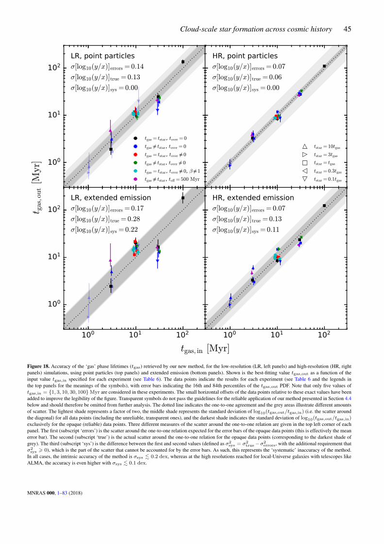
Cloud-scale star formation across cosmic history 45
100
101
102LR, point particlesσ[log10(y/x)]errors = 0.14
σ[log10(y/x)]true = 0.13
σ[log10(y/x)]sys = 0.00
tgas = tstar, tover = 0
tgas tstar, tover = 0
tgas = tstar, tover 0
tgas tstar, tover 0
tgas = tstar, tover 0, β 1
tgas tstar, toff = 500 Myr
HR, point particlesσ[log10(y/x)]errors = 0.07
σ[log10(y/x)]true = 0.06
σ[log10(y/x)]sys = 0.00
tstar = 10tgas
tstar = 3tgas
tstar = tgas
tstar = 0.3tgas
tstar = 0.1tgas
100 101 102
100
101
102LR, extended emissionσ[log10(y/x)]errors = 0.17
σ[log10(y/x)]true = 0.28
σ[log10(y/x)]sys = 0.22
100 101 102
HR, extended emissionσ[log10(y/x)]errors = 0.07
σ[log10(y/x)]true = 0.13
σ[log10(y/x)]sys = 0.11
tgas, in [Myr]
t gas,o
ut [
Myr]
Figure 18. Accuracy of the ‘gas’ phase lifetimes (tgas) retrieved by our new method, for the low-resolution (LR, left panels) and high-resolution (HR, rightpanels) simulations, using point particles (top panels) and extended emission (bottom panels). Shown is the best-fitting value tgas,out as a function of theinput value tgas,in specified for each experiment (see Table 6). The data points indicate the results for each experiment (see Table 6 and the legends inthe top panels for the meanings of the symbols), with error bars indicating the 16th and 84th percentiles of the tgas,out PDF. Note that only five values oftgas,in = {1, 3, 10, 30, 100}Myr are considered in these experiments. The small horizontal offsets of the data points relative to these exact values have beenadded to improve the legibility of the figure. Transparent symbols do not pass the guidelines for the reliable application of our method presented in Section 4.4below and should therefore be omitted from further analysis. The dotted line indicates the one-to-one agreement and the grey areas illustrate different amountsof scatter. The lightest shade represents a factor of two, the middle shade represents the standard deviation of log10(tgas,out/tgas,in) (i.e. the scatter aroundthe diagonal) for all data points (including the unreliable, transparent ones), and the darkest shade indicates the standard deviation of log10(tgas,out/tgas,in)
exclusively for the opaque (reliable) data points. Three different measures of the scatter around the one-to-one relation are given in the top left corner of eachpanel. The first (subscript ‘errors’) is the scatter around the one-to-one relation expected for the error bars of the opaque data points (this is effectively the meanerror bar). The second (subscript ‘true’) is the actual scatter around the one-to-one relation for the opaque data points (corresponding to the darkest shade ofgrey). The third (subscript ‘sys’) is the difference between the first and second values (defined as σ2
sys = σ2true−σ2
errors, with the additional requirement thatσ2
sys > 0), which is the part of the scatter that cannot be accounted for by the error bars. As such, this represents the ‘systematic’ inaccuracy of the method.In all cases, the intrinsic accuracy of the method is σsys . 0.2 dex, whereas at the high resolutions reached for local-Universe galaxies with telescopes likeALMA, the accuracy is even higher with σsys . 0.1 dex.
MNRAS 000, 1–83 (2018)

46 J. M. D. Kruijssen et al.
solved in observed galaxy maps, because the observational pointspread function typically resembles a Gaussian (see Section 5).However, it is possible (e.g. due to substructure, blending, highly-resolved independent regions, or a different point spread or smooth-ing function19) that the assumption of Gaussian surface densityprofiles is invalid. In this case, the measured time-scales may bea bad representation of the true evolutionary timeline.
The bottom panels of Figure 18 demonstrate that any devia-tions resulting from the above assumptions is modest. The excessof the scatter beyond the mean error bar size (which is a measurefor the inaccuracy of the method) indeed increases, but it remainswithin reasonable limits. The experiments using high-resolutionextended emission maps have a spatial resolution that is comfort-ably obtained with ALMA. For these experiments, the excess scat-ter around the one-to-one relation is 0.11 dex (which is less than30 per cent). While this residual scatter is non-zero, it is an encour-aging accuracy given the discussed assumptions. It is also sufficientfor astrophysical purposes. Current discussions in the literature re-garding the molecular cloud lifetime discuss order-of-magnitudedifferences (e.g. Dobbs et al. 2014; Jeffreson & Kruijssen 2018),which our method can plausibly distinguish at the > 8σ level.
4.2.3.3 General conclusions We see that across all panels ofFigure 18, the largest outliers (ignoring the transparent symbols)are upward or downward-pointing triangles. These symbols repre-sent the experiments in which tstar and tgas differ by a factor of10. Throughout the experiments carried out for this study (also seeSection 4.3.4), we have noticed that the most accurate results areobtained when tstar and tgas are similar. This occurs because the‘tuning fork’ diagram of Figure 2 becomes asymmetric for dissim-ilar values of tstar and tgas, which moves one of the two branchesin the diagram closer to the B = 1 line, where the shape of thediagram becomes less sensitive to the underlying time-scales. Thiscan limit the accuracy of the method.
To optimize the reliability of the results, the tracer for whichthe time-scale is known (i.e. the ‘reference’ time-scale, which inpractice will often refer to the star formation tracer lifetime tstar)should be chosen to be as similar as possible to the measured time-scale (which in practice will often refer to the cloud lifetime tgas).This may require iteration or running multiple experiments withdifferent reference maps (e.g. using Hα, FUV, and NUV, see Hay-don et al. 2018) to converge on the best tracer to use. Figure 18shows that the inaccuracy of the upward and downward-pointingtriangles is not unacceptable – the deviations from the one-to-onerelation are generally less than a factor of two and there are severalsuch symbols that lie right on top of the one-to-one relation. How-ever, larger deviations would begin to impede astrophysical appli-cations of the method. For practical applications, we therefore rec-ommend an a posteriori evaluation to discard results for which thedifference between tstar and tgas exceeds an order of magnitude.By contrast, time-scale measurements can be considered reliablewhen | log10(tstar/tgas)| 6 1.
4.2.4 Accuracy of the ‘feedback time-scale’ tover
The second test carried out using the 88 experiments from Sec-tion 4.2.2 is to determine how well the duration of the ‘overlap’phase (tover) is retrieved by our method. Like tgas before, tover can
19 We note that the shape of the Wendland C4 smoothing kernel used hereto generate the maps is very similar to a Gaussian.
have a variety of physical meanings depending on the gas and starformation tracers used. For the specific, real-Universe example oftracing (molecular) gas with CO and star formation with an ioniza-tion tracer like Hα, this quantity refers to the time it takes the COemission from a molecular cloud to disappear once the first ionis-ing photons have started to emerge from the embedded star-formingregion. We refer to this duration as the feedback time-scale. Anal-ogously to Section 4.2.3, we obtain the complete PDF of tover andshow the best-fitting value of tover (referred to as tover,out) as afunction of the input value of tover from Table 6 (referred to astover,in) for all 88 experiments in Figure 19. On both axes, we nor-malise tover to the total duration of the timeline τ , thus comparingthe input fraction of a region’s lifetime during which it is visible inboth maps to the retrieved fraction.
4.2.4.1 Point particles As in Section 4.2.3, we expect the pointparticle experiments to yield the best results, owing to the straight-forward identification of independent regions. The top panels ofFigure 19 indeed demonstrate good agreement, with standard de-viations around the one-to-one relation (σtrue) of 2–4 per cent intover/τ . In both cases, this scatter is larger than expected based onthe errors, indicating that there is a systematic uncertainty associ-ated with the method. This uncertainty does not take the form of asystematic bias, but represents an increase of the statistical uncer-tainty. As previously, there are two possible sources of the addedscatter. Firstly, it is possible that the substructure in the spatial dis-tribution of regions somehow influences tover more strongly thantgas (on which the influence for the amount of substructure in thesesimulations is negligible, see Section 4.2.3). Secondly, deviationsfrom a constant SFR could lead to biases in the measurements oftover. This should affect tover more strongly than tgas, because itcovers a shorter duration and thus is more susceptible to Poissonnoise.
We test the hypothesis that variations in the SFR are respon-sible for the main outliers in the top panels of Figure 19. In theleft-hand panel, the main outlier is experiment 13 (the red squareat {tover,in/τin, tover,out/τout} = {0.11, 0.05}), whereas in theright-hand panel, the main outliers are experiments 14, 18, 19,and 20 (the cluster of squares at {tover,in/τin, tover,out/τout} ={0.25, 0.16}). The latter four experiments cover the same age binsand only differ in terms of the overlap-to-isolated flux ratios βstar
and βgas (see Section 4.2.5). The fact that these four points showan almost identical discrepancy compared to the input values whilesharing the same timeline coverage strongly suggests that SFR vari-ations are the cause of their deviation. We verify this by compar-ing the fraction fM (tover) of the total stellar mass in each mapformed during tover to the corresponding time fractions tover,in/τinand tover,out/τout. If SFR variations cause the observed offsets,then fM (tover) should match the measured value of tover,out/τout
rather than the stellar mass fraction expected for a constant SFRtover,in/τin.
For experiment 13 in the top-left panel of Figure 19, we findthat fM (tover) = 0.05, whereas for the cluster of points around ex-periment 14 in the top-right panel, we find that fM (tover) = 0.16.Within the displayed precision, both of these numbers are identi-cal to the retrieved values of tover,out/τout (0.05 and 0.16, respec-tively). Therefore, we conclude that the systematic uncertainty ofσsys = 2–4 per cent identified in the top panels of Figure 19 iscaused by deviations from a constant SFR during the covered partof the timeline. This is a real effect that will also affect observa-tional applications of our method. Assuming that the simulationsconsidered in this paper provide a reasonable representation of SFR
MNRAS 000, 1–83 (2018)

Cloud-scale star formation across cosmic history 47
0.0
0.2
0.4
0.6
0.8
1.0 LR, point particlesσ(y− x)errors = 0.01
σ(y− x)true = 0.02
σ(y− x)sys = 0.02
tgas = tstar, tover = 0
tgas tstar, tover = 0
tgas = tstar, tover 0
tgas tstar, tover 0
tgas = tstar, tover 0, β 1
tgas tstar, toff = 500 Myr
HR, point particlesσ(y− x)errors = 0.00
σ(y− x)true = 0.04
σ(y− x)sys = 0.04
tstar = 10tgas
tstar = 3tgas
tstar = tgas
tstar = 0.3tgas
tstar = 0.1tgas
0.0 0.2 0.4 0.6 0.8 1.0
0.0
0.2
0.4
0.6
0.8
1.0
.combination of
real physical excessand region blending
LR, extended emissionσ(y− x)errors = 0.03
σ(y− x)true = 0.06
σ(y− x)sys = 0.05
0.0 0.2 0.4 0.6 0.8 1.0
HR, extended emissionσ(y− x)errors = 0.01
σ(y− x)true = 0.06
σ(y− x)sys = 0.06
tover, in/τin
t over,o
ut/τ o
ut
Figure 19. Accuracy of the ‘overlap’ phase lifetimes (tover) retrieved by our new method, normalised to the total duration of the timeline (τ ), for the low-resolution (LR, left panels) and high-resolution (HR, right panels) simulations, using point particles (top panels) and extended emission (bottom panels).Shown is the best-fitting value tover,out/τout as a function of the input value tover,in/τin specified for each experiment (see Table 6). The data pointsindicate the results for each experiment (see Table 6 and the legends in the top panels for the meanings of the symbols), with error bars indicating the 16th and84th percentiles of the tover,out/τout PDF. Note that only four values of tover,in/τin = {0, 0.11, 0.25, 0.67} are considered in these experiments. The smallhorizontal offsets of the data points relative to these exact values have been added to improve the legibility of the figure. Transparent symbols do not pass theguidelines for the reliable application of our method presented in Section 4.4 below and should therefore be omitted from further analysis. The red ellipses andannotation in the bottom panels indicate real outliers that are not due to any inaccuracy of the method (part of this tover/τ excess is caused by the fact that theextended emission maps contain peaks consisting of multiple particles that have a non-zero age spread, see the text). The dotted line indicates the one-to-oneagreement and the grey areas illustrate different amounts of scatter. The lightest shade represents a scatter of 0.1 (i.e. 10 per cent of the timeline durationτ ), the middle shade represents the standard deviation of tover,out/τout − tgas,in/τin (i.e. the scatter around the diagonal) for all data points (includingthe unreliable, transparent ones), and the darkest shade indicates the standard deviation of tover,out/τout − tgas,in/τin exclusively for the opaque (reliable)data points. Three different measures of the scatter around the one-to-one relation are given in the top left of each panel. The first (subscript ‘errors’) is thescatter around the one-to-one relation expected for the error bars of the opaque data points (this is effectively the mean error bar). The second (subscript ‘true’)is the actual scatter around the one-to-one relation for the opaque data points (corresponding to the darkest shade of grey). The third (subscript ‘sys’) is thedifference between the first and second values (defined as σ2
sys = σ2true − σ2
errors, with the additional requirement that σ2sys > 0), which is the part of the
scatter that cannot be accounted for by the error bars. As such, this represents the ‘systematic’ inaccuracy of the method. The intrinsic accuracy of the methodis σsys . 0.05 (see the text), implying that tover can be determined to about 5 per cent of τ . Any tover < 0.05τ is therefore consistent with tover = 0.
MNRAS 000, 1–83 (2018)

48 J. M. D. Kruijssen et al.
variations in disc galaxies, we recommend a minimum uncertaintyof 5 per cent in tover/τ , even if the formal error is smaller. In prac-tice, this means that tover/τ < 0.05 is consistent with no over-lap and tover/τ > 0.95 is consistent with completely overlappingphases.
4.2.4.2 Extended emission Contrary to the good performanceof the method in retrieving tover/τ when applying it to the pointparticle maps in the top panels of Figure 19, the bottom panels ofFigure 19 show a group of experiments with measured values oftover that are significantly higher than the input values (highlightedby the light red ellipses). This excess of tover only occurs in some(but not all) of the experiments with low tover,in/τin. While thisdeviation from the one-to-one relation may look like a major inac-curacy of the method at first sight, it is largely physical in nature.
When determining how well tover is retrieved from the ex-tended emission maps discussed in Figure 17, it is important torealise that only the point particle maps may exhibit one-to-oneagreement between input and output. In these maps, it is possi-ble to control the value of tover by specifying the age ranges forwhich the particles are included in the map, because individual starparticles have a single formation time. This does not hold for theextended emission maps, because their independent regions con-sist of groups of star particles that have a non-zero, intrinsic agespread – the star formation history of each progenitor cloud is nota delta function. As a result, the descendant groups of star particlesmay be present in both maps even in the experiments for which wespecify tover,in = 0. Therefore, any value of tover retrieved fromthe extended emission maps should correspond to the sum of thenumber specified in Table 6 and the age spread of each region. Thisexplains why mostly experiments with low tover,in/τin show thetover excess. In these experiments, the intrinsic age spread of theregions in the simulation is more likely to dominate over the im-posed age spread tover,in.
It is important to realise that tover can only contain an intrin-sic age spread for regions that consist of a sufficient number of starparticles to sample this age spread. In practice, the mean numberof particles per region depends on the total duration of each phase.A very rough estimate of this number can be made by dividing thenumber of regions in the point particle experiments by the numberof regions in the extended emission experiments (cf. the tables inAppendix D1). A minimum of two particles per region is requiredfor both tracers to sample any age spread at all. This is only con-sistently achieved in experiments 3 and 4 (see Table 6), where theduration of both phases exceeds 30 Myr and the mean number ofstar particles per region is 4–15 for each phase. The other experi-ments have less than two particles per region on average, implyingthat the age spread is only resolved in a subset of the regions in themap. This dependence on the numerical sampling implies that theexcess of tover depends on the total duration of the timeline, andis only fully included in experiments 3 and 4. For phase durationsshorter than∼ 30 Myr, the tover excess is smaller than the true agespread, because the likelihood of sampling the timeline with a suf-ficient number of particles to cover the full overlap phase is smallerthan unity.
We reiterate that the above increase of the intrinsic age spreadwith the total duration of the timeline is entirely numerical in natureand results from the quantisation of the mass reservoir into particlesof 1.4 × 10⁴ M� (low resolution) and 2.7 × 10³ M� (high reso-lution). In real star-forming regions, this type of quantisation couldpotentially take place in ionization-based star formation tracerssuch as Hα, because such emission is generated by individual mas-
sive stars. However, such a quantisation will have a much weakereffect than in our simulations, because roughly one O-star is formedper 100 M�, assuming a normal IMF (e.g. Chabrier 2003). A sin-gle star particle in our high-resolution simulation would host 27 O-stars, i.e. the sampling rate of a real star-forming region is a factorof ∼ 30 higher, meaning that an age spread like the one we see inthe simulations would be well-sampled already for tstar ∼ 1 Myrrather than the limit of tstar ∼ 30 Myr that we see in the exper-iments. The commonly-used star formation tracers Hα, FUV, andNUV all cover time-scales well in excess of 1 Myr (Haydon et al.2018). Therefore, we conclude that the method is capable of accu-rately retrieving the overlap (or feedback) time-scale from observed(molecular) gas and star formation tracer maps.
The bottom panels of Figure 19 contain two additional trans-parent data points (indicative of not satisfying the guidelines for thereliable application of our method presented in Section 4.4 below)relative to those in Figure 18. These are the largest outliers in thebottom-right panel and correspond to experiments 3 and 4, whichhave large-to-extreme tover excesses of tover,out = 4.87+0.58
−0.62 Myrand tover,out = 39.27+3.13
−2.74 Myr, respectively. Visual inspectionof the maps reveals extreme blending of the regions, caused by thelong timelines covered by these experiments (see Table 6) and theresulting high spatial density of the regions. The large discrepancybetween the input and output value of tover in these experimentshighlights that blending can negatively affect the accuracy of mea-suring tover with our method.
Interestingly, blending does not influence the accuracy of thetgas measurements in Section 4.2.3, because it affects both phasesof the timeline in Figure 1 in proportion to their number densitiesin the maps and therefore in proportion to their durations, result-ing in the same relative change of either time-scale. Fundamen-tally, our method measures the relative time-scale difference be-tween both phases, implying that the measurement of tgas is notaffected by blending. However, this does not hold when measur-ing tover, because that quantity is obtained by measuring the cor-relation between both phases in excess of the statistical correlationexpected for a random distribution in the plane. It is easy to pic-ture the influence of blending on this measurement with an exam-ple. If one would convolve both the stellar and ‘gas’ maps with apoint spread function that matches the size of the simulated galaxy,both phases would be fully correlated in the convolved maps andthe ratio between both maps would equal the galactic average ev-erywhere. Naturally, this should result in a duration of the overlapphase equal to the total duration of the timeline, irrespective of whatthe true duration of the overlap phase would have been in the un-convolved maps. This extreme example shows that blending addsto the true time overlap between the phases.
In order to minimize the effects of blending on the measure-ment of tover with our method, two potential effects should be ac-counted for. Firstly, blending can inhibit the identification of inde-pendent regions, because the blending decreases the contrast be-tween the flux density minimum in between adjacent peaks and thepeaks themselves. For a logarithmic spacing δ log10 F between theflux levels used to identify peaks (see Section 3), there exists a min-imum distance between the peaks (in units of the peak radius) suchthat they can still be identified. The mathematical derivation of thisdistance is provided in Appendix B, but here we give the ratiosbetween the separation lengths and the peak radius needed to iden-tify the peaks in our experiments. For the {low, high} resolutionsimulations, we use a logarithmic spacing of δF = {0.25, 0.5},which requires that λ/r > {3.14, 3.84} or, when expressed in
MNRAS 000, 1–83 (2018)

Cloud-scale star formation across cosmic history 49
terms of the region concentration parameter ζ ≡ 2r/λ, requiresthat ζ < {0.64, 0.52}.
Secondly, the blending of adjacent peaks also causes the emis-sion of each individual region to be increased by some factor. Thisleads to an overestimation of the duration of the overlap phase, be-cause blending combines the emission from regions with indepen-dent (and therefore most likely different) ages into a single region.We quantify this effect in Appendix B, where we consider two ad-jacent, two-dimensional Gaussian peaks and calculate as a functionof λ/r which fraction of the emission on one side of the equidis-tance line is constituted by contamination from the neighbour. Thisfraction steeply decreases as a function of distance and should belower than the desired accuracy of the tover measurement. The toppanels of Figure 19 demonstrate that the intrinsic accuracy of themethod is∼ 0.05 in tover/τ due to deviations from a constant SFR.Therefore, it is desirable that much less than 5 per cent of the emis-sion in any region comes from neighbouring emission peaks. Thecondition that peaks are separated by ∼ 1.7 times their FWHM(corresponding to λ/r > 4 or ζ ≡ 2r/λ < 0.5) results in acontamination percentage of ∼ 5 per cent. This satisfies the aboverequirements and we will use this condition to determine if blend-ing may have influenced the measurements of tover. If regions aremarginally resolved, this requirement translates to having a resolu-tion (FWHM) of λ/1.7 or better. This is discussed further in Sec-tion 4.3.6, where we carry out resolution tests designed to explorethese issues further.
The above upper limits on ζ (and hence blending) successfullyidentify experiments 3 and 4 in the bottom-right panel of Figure 19as an inaccurate measurement of the duration of the overlap phase.It also successfully identifies several of the experiments using thereal gas maps of the simulations in Section 4.3 below, which uponvisual inspection are all clearly affected by blending as well. How-ever, it fails to identify experiments 4 and 21 in the bottom-leftpanel of Figure 19, which also have large tover excesses due toblending. We expect that this is caused by a large radial variationof ζ within the maps, which implies that the mean ζ is not repre-sentative for a non-negligible fraction of the regions, especially to-wards the inner galaxy. Therefore, we recommend to always carryout a visual inspection of the maps to verify if they show any regionblending. This is particularly useful because the measured value ofζ is an average over the entire map. If there is substantial spatialvariation of ζ (e.g. as a function of galactocentric radius), then itis possible that blending can only be identified by visual inspec-tion, after which parts of the maps may be masked to obtain a morehomogeneous and representative measurement of ζ. We have ex-panded the method with a new way of filtering out emission onsize scales exceeding the region separation length λ (Hygate et al.2018), which will help to avoid blending without human interven-tion.
4.2.4.3 General conclusions In summary, we see that themethod is capable of measuring the fraction of the timeline inwhich both phases overlap (tover/τ ) with an accuracy of about 0.05or 5 per cent. A higher accuracy could be obtained in principle, butfluctuations of the SFR imply that our assumption of a constantSFR is violated, thus limiting the attainable accuracy. We proposethat the above accuracy is appropriate for disc galaxies, but will nat-urally be worse in systems with strongly varying SFRs, i.e. starburstsystems like dwarf galaxies or mergers. Should the star formationhistory of the observed field be known over the entire duration ofthe timeline τ (e.g. by stellar population synthesis fitting), then itis possible to correct the time-scales retrieved by our method for
variations in the SFR over the fraction of the timeline covered bythe stellar phase.
The method’s accuracy may be decreased if no measures aretaken to avoid the blending of regions in the tracer maps used. Forthis reason, we recommend that max (ζstar, ζgas) < ζcrit (to al-low the regions to be identified by the clump finding algorithm; seeAppendix B for the derivation of ζcrit as a function of δ log10 F)and max (ζstar, ζgas) < 0.5 (to avoid the contamination of peaksby nearby regions). In case of a strong spatial variation of ζ acrosseither of the maps, we recommend to carry out a visual inspectionto verify the degree of blending and to mask the maps if neces-sary, or to filter out diffuse emission on size scales larger than λ(Hygate et al. 2018). If any of these conditions is not satisfied andregion blending does affect the analysis, then the measured valueof tover is not necessarily incorrect, but it reflects the duration forwhich both tracers coexist at the blending scale. This compositevalue of tover may then exceed the ‘Lagrangian’ duration of theoverlap phase when following an individual region through its evo-lution.
As discussed at the beginning of this section, we expect thatreal-Universe applications of the method’s ability to constrain theduration of the overlap phase will help provide insight in (molec-ular cloud destruction by) stellar feedback. Of course, the physicalmeaning of tover depends on the adopted tracers. In the example oftracing (molecular) gas with CO and star formation with Hα, tover
corresponds to the feedback time-scale, i.e. the time over which ex-cess CO emission disappears once ionising photons start to escapefrom a region.
In order to distinguish between various feedback mechanisms,it is essential that the accuracy of the tover measurement allows re-solving the time-scale differences expected between these mecha-nisms. For instance, ruling out SNe in favour of early (e.g. pho-toionization) feedback would require an accuracy of the order3 Myr. In view of the expected ∼ 5 per cent accuracy in tover/τ ,this example would necessitate the use of gas and star formationtracers that together cover τ < 60 Myr. This can be ensured byadopting tracers with short lifetimes, e.g. Hα (which contributeststar ∼ 5 Myr, Haydon et al. 2018) to trace star formation. Con-trary to some star formation tracers, the lifetime of the molecu-lar gas tracer is not known a priori. If the molecular gas tracer[e.g. 12CO(1–0) or 12CO(2–1)] turns out to be longer-lived thantgas ∼ 50 Myr, one can probe feedback-driven gas dispersal byswitching to a higher-density gas tracer such as 13CO(1–0) or HCN(e.g. Leroy et al. 2017), which are expected to have much shorterlifetimes. In addition to using the time-scale associated with ion-ising photons to determine which feedback mechanism is respon-sible for molecular cloud destruction, it should be possible to dis-tinguish between feedback mechanisms in even more detail if addi-tional tracers can be identified that are associated with single mech-anisms (see Section 8.2). Combining the above considerations, ourmethod should then allow measurements of the feedback time-scalein galaxies with an accuracy better than 1 Myr, which is sufficientto distinguish between several of the possible feedback mecha-nisms. The above distinctions between feedback mechanisms sharethe benefit of not depending on feedback models. However, it willalso be possible to directly compare the cloud destruction time-scales predicted for individual feedback mechanisms (or combina-tions thereof) to measurements of tover obtained with our method.
MNRAS 000, 1–83 (2018)

50 J. M. D. Kruijssen et al.
Table 7. Mean best-fitting values of β using age-binned stellar maps
Runs 〈βstar〉1.0 〈βstar〉0.5 〈βgas〉1.0 〈βgas〉0.5
LR points 0.99+0.03−0.02 0.52+0.04
−0.02 0.94+0.04−0.03 0.48+0.02
−0.00
HR points 0.98+0.01−0.00 0.50+0.01
−0.00 0.93+0.01−0.01 0.47+0.01
−0.00
LR extended 0.95+0.26−0.11 0.55+0.09
−0.05 1.12+0.39−0.10 0.87+0.03
−0.02
HR extended 1.02+0.03−0.03 0.74+0.03
−0.04 0.91+0.03−0.02 0.62+0.05
−0.04
4.2.5 Accuracy of the overlap-to-isolated flux ratio β
Next to the gas phase lifetime tgas and the duration of the overlapphase tover, our method also measures the mean flux ratio betweenregions in the overlap phase to those not in the overlap phase (whichwe refer to as being ‘isolated’ in time rather than spatially). Thisoverlap-to-isolated flux ratio β is calculated for both tracers, im-plying that we have measurements of βstar and βgas. As discussedin Section 3 and KL14, knowledge of this flux ratio is sufficient toaccount for the effect of the flux evolution history of either traceron the retrieved time-scales. In Table 6, all experiments with a non-zero value of tover result in a meaningful measurement of βstar andβgas. For most experiments, we have set both quantities to unity,but experiments 18–20 are chosen to explore the effects of varyingβ on the best-fitting quantities.
Table 7 shows the mean obtained values of βstar and βgas
for different subsets of experiments. We divide up the experimentsin the four types of Figure 17, i.e. low-resolution point particles,high-resolution point particles, low-resolution extended emission,and high-resolution extended emission. For each of these, the meanoutput values of βstar and βgas are calculated for the experimentswhere the input values are set to unity (columns indicated by〈β〉1.0) and to 0.5 (columns indicated by 〈β〉0.5). We only con-sider experiments for which tover,in > 0. As expected, the valuesof βstar and βgas in the point particle experiments are in excellentagreement with the input values. This shows that the method is ca-pable of capturing the mean flux evolution of independent regionsby correctly retrieving the overlap-to-isolated flux ratio, even if theerror bars may be underestimated by up to a factor of 2.20. Forthe extended emission experiments with input value β = 0.5, theagreement is generally poor. However, as in Section 4.2.4, this is areal effect rather than a flaw in the method, because the regions inthe extended emission maps consist of collections of particles. Thismeans that it is no longer possible to control which particles re-side in the overlap phase, implying that the overlap-to-isolated fluxratio of these composite regions should be in the range β = 0.5–1.0. Table 7 shows that this is indeed the case to within the errorbars. While this broad range clearly shows that the extended emis-sion experiments provide no particularly strong test of the method’saccuracy in retrieving the overlap-to-isolated flux ratios βstar andβgas, it is encouraging that the output values are consistent with theexpected range.
4.3 Gas and stellar maps
Our second set of tests is based on maps of both the gas and thestar particles in the simulations. Having established the accuracy ofthe method with the controlled experiments of Section 4.2, we can
20 We obtain this factor by considering that across eight numbers, only twoor three should deviate by more than 1σ, whereas currently this applies tohalf of the measurements. Increasing the error bars by a factor of 2 wouldresult in two numbers deviating by more than 1σ.
now turn to a more realistic set of experiments. By using the actualdistributions of gas particles in the simulations and combining thesewith the ‘age-binned’ stellar maps as before, we can investigatedependences that may affect practical applications of the methodto observations. Specifically, we consider the effects of
(i) diffuse emission in the maps, i.e. emission emerging fromscales > λ;
(ii) the (stellar) reference time-scale, reflecting the star forma-tion tracer used (e.g. Leroy et al. 2012; Haydon et al. 2018);
(iii) the volume density threshold above which the gas is visible,reflecting the gas tracer used (e.g. Shirley 2015; Leroy et al. 2017);
(iv) the spatial resolution, reflecting the observational setup andthe target distance or redshift;
(v) the galaxy inclination angle;(vi) the number of independent regions in the maps, represented
by the identified number of peaks.
4.3.1 Procedure for creating the maps
For the experiments discussed here, the age-binned maps of thestar particles are generated for different age ranges in exactly thesame way as described in Section 4.2.1. To generate maps of thegas particles in the galaxy models, we first need to define the min-imum volume densities above which the particles are displayed.In the phase diagrams of Figure 16, vertical white lines indicatevolume densities of ρ = {0.5, 1, 2} cm−3 (low resolution) andρ = {1, 2, 4} cm−3 (high resolution). As shown by the hatched re-gion, these critical densities provide a reasonable match to the min-imum density for particles to become star-forming (ρ = 0.7 cm−3)and together span roughly an order of magnitude, across whichdifferent fractions of the star-forming ISM are traced. Therefore,we use the three volume densities indicated in each panel of Fig-ure 16 to generate the gas particle maps, where the central valuesof ρmin,LR = 1 cm−3 (low resolution) and ρmin,HR = 2 cm−3
(high resolution) act as the default choices.In addition to the above reference time-scales tstar and min-
imum gas volume densities ρmin, we specify two other quantitiesthat are investigated here. Firstly, the spatial resolution of the mapsis specified by changing lap,min in Table 2 and settingNap such thatthe other aperture sizes remain unchanged. For instance, to changethe spatial resolution to 200 pc instead of the default 50 pc, we setlap,min = 200 pc and Nap = 6 (instead of the default Nap = 8)to retain the same aperture size spacing as before. Secondly, wevary the inclination angle of the galaxy maps. This is achieved byrotating the simulation output around the x-axis by an angle in therange i = [0, 90]◦ prior to generating the maps. The remainingquantities of interest (diffuse emission fraction and number of in-dependent regions) are not specified, but vary sufficiently acrossthe set of experiments to draw meaningful conclusions about theirinfluence on the results. We note that out of the quantities used togenerate the maps, only tstar and i are used as input parameters inthe method of Section 3. The method is not informed of the valuesof the other quantities. Having said that, the choice of stellar andgas tracer (each associated with their own time-scale or minimumdensity, respectively) needs to be considered when setting the inputparametersXstar andXgas for converting between pixel values andSFR and gas mass.
Having defined the subsets of particles that are shown in eachmap, we generate the surface density maps of these particles asdescribed in Section 4.2.1. The maps are square with a projecteddiameter of 20 kpc and 1403 pixels, corresponding to a projected
MNRAS 000, 1–83 (2018)
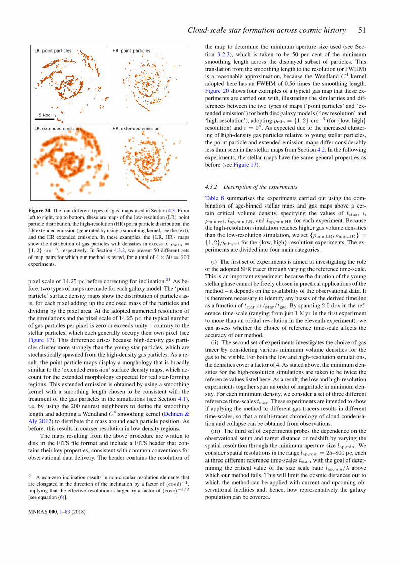
Cloud-scale star formation across cosmic history 51
LR, point particles
5 kpc
HR, point particles
LR, extended emission HR, extended emission
Figure 20. The four different types of ‘gas’ maps used in Section 4.3. Fromleft to right, top to bottom, these are maps of the low-resolution (LR) pointparticle distribution, the high-resolution (HR) point particle distribution, theLR extended emission (generated by using a smoothing kernel, see the text),and the HR extended emission. In these examples, the {LR, HR} mapsshow the distribution of gas particles with densities in excess of ρmin =
{1, 2} cm−3, respectively. In Section 4.3.2, we present 50 different setsof map pairs for which our method is tested, for a total of 4 × 50 = 200experiments.
pixel scale of 14.25 pc before correcting for inclination.21 As be-fore, two types of maps are made for each galaxy model. The ‘pointparticle’ surface density maps show the distribution of particles as-is, for each pixel adding up the enclosed mass of the particles anddividing by the pixel area. At the adopted numerical resolution ofthe simulations and the pixel scale of 14.25 pc, the typical numberof gas particles per pixel is zero or exceeds unity – contrary to thestellar particles, which each generally occupy their own pixel (seeFigure 17). This difference arises because high-density gas parti-cles cluster more strongly than the young star particles, which arestochastically spawned from the high-density gas particles. As a re-sult, the point particle maps display a morphology that is broadlysimilar to the ‘extended emission’ surface density maps, which ac-count for the extended morphology expected for real star-formingregions. This extended emission is obtained by using a smoothingkernel with a smoothing length chosen to be consistent with thetreatment of the gas particles in the simulations (see Section 4.1),i.e. by using the 200 nearest neighbours to define the smoothinglength and adopting a Wendland C4 smoothing kernel (Dehnen &Aly 2012) to distribute the mass around each particle position. Asbefore, this results in coarser resolution in low-density regions.
The maps resulting from the above procedure are written todisk in the FITS file format and include a FITS header that con-tains their key properties, consistent with common conventions forobservational data delivery. The header contains the resolution of
21 A non-zero inclination results in non-circular resolution elements thatare elongated in the direction of the inclination by a factor of (cos i)−1,implying that the effective resolution is larger by a factor of (cos i)−1/2
[see equation (6)].
the map to determine the minimum aperture size used (see Sec-tion 3.2.3), which is taken to be 50 per cent of the minimumsmoothing length across the displayed subset of particles. Thistranslation from the smoothing length to the resolution (or FWHM)is a reasonable approximation, because the Wendland C4 kerneladopted here has an FWHM of 0.56 times the smoothing length.Figure 20 shows four examples of a typical gas map that these ex-periments are carried out with, illustrating the similarities and dif-ferences between the two types of maps (‘point particles’ and ‘ex-tended emission’) for both disc galaxy models (‘low resolution’ and‘high resolution’), adopting ρmin = {1, 2} cm−3 (for {low, high}resolution) and i = 0◦. As expected due to the increased cluster-ing of high-density gas particles relative to young stellar particles,the point particle and extended emission maps differ considerablyless than seen in the stellar maps from Section 4.2. In the followingexperiments, the stellar maps have the same general properties asbefore (see Figure 17).
4.3.2 Description of the experiments
Table 8 summarises the experiments carried out using the com-bination of age-binned stellar maps and gas maps above a cer-tain critical volume density, specifying the values of tstar, i,ρmin,ref , lap,min,LR, and lap,min,HR for each experiment. Becausethe high-resolution simulation reaches higher gas volume densitiesthan the low-resolution simulation, we set {ρmin,LR, ρmin,HR} ={1, 2}ρmin,ref for the {low, high}-resolution experiments. The ex-periments are divided into four main categories.
(i) The first set of experiments is aimed at investigating the roleof the adopted SFR tracer through varying the reference time-scale.This is an important experiment, because the duration of the youngstellar phase cannot be freely chosen in practical applications of themethod – it depends on the availability of the observational data. Itis therefore necessary to identify any biases of the derived timelineas a function of tstar or tstar/tgas. By spanning 2.5 dex in the ref-erence time-scale (ranging from just 1 Myr in the first experimentto more than an orbital revolution in the eleventh experiment), wecan assess whether the choice of reference time-scale affects theaccuracy of our method.
(ii) The second set of experiments investigates the choice of gastracer by considering various minimum volume densities for thegas to be visible. For both the low and high-resolution simulations,the densities cover a factor of 4. As stated above, the minimum den-sities for the high-resolution simulations are taken to be twice thereference values listed here. As a result, the low and high-resolutionexperiments together span an order of magnitude in minimum den-sity. For each minimum density, we consider a set of three differentreference time-scales tstar. These experiments are intended to showif applying the method to different gas tracers results in differenttime-scales, so that a multi-tracer chronology of cloud condensa-tion and collapse can be obtained from observations.
(iii) The third set of experiments probes the dependence on theobservational setup and target distance or redshift by varying thespatial resolution through the minimum aperture size lap,min. Weconsider spatial resolutions in the range lap,min = 25–800 pc, eachat three different reference time-scales tstar, with the goal of deter-mining the critical value of the size scale ratio lap,min/λ abovewhich our method fails. This will limit the cosmic distances out towhich the method can be applied with current and upcoming ob-servational facilities and, hence, how representatively the galaxypopulation can be covered.
MNRAS 000, 1–83 (2018)

52 J. M. D. Kruijssen et al.
(iv) The fourth set of experiments varies the galaxy inclinationangle i to identify any corresponding limits on the applicabilityof our method. As before, we consider three different referencetime-scales for each inclination angle. This set of experiments isexpected to show some degeneracy with the third set (spatial reso-lution), because increasing the inclination results in an increase ofthe effective resolution scale by a factor of (cos i)−1/2.
As outlined in Section 4.3.1, we additionally investigate how theaccuracy of the results changes as a function of the number of in-dependent regions hosted in each of the maps and make a first esti-mate of how diffuse emission affects the results (this latter depen-dence will be quantified in more detail by Hygate et al. 2018). Bothof these are relevant tests for applications of our method to obser-vations. The diffuse fraction cannot always be controlled a priori(e.g. Pety et al. 2013; Caldu-Primo & Schruba 2016) and obtainingan understanding of its effects is thus important. By contrast, if wecan identify a minimum number of independent regions needed forreliable applications of the method, this can be an important driverfor choosing the spatial coverage in observational campaigns.
The above sets of experiments are carried out using the ‘pointparticle’ or the ‘extended emission’ surface density maps (see Sec-tion 4.3.1), both for the low and high-resolution simulations. Wethus have a total of 200 experiments using pairs of age-binned stel-lar maps and gas maps. Some of the parameters used in these ex-periments deviate from the default values in Section 3. Firstly, theinclinations and spatial resolutions (i.e. minimum aperture sizes)of the maps vary on a case-by-case basis, as shown by Table 8. Wetherefore adjust i, lap,min, and Nap accordingly for each experi-ment. Secondly, we adjust the range of galactocentric radii to avoidlarge empty areas in the maps and set Rmax = 10 kpc (7 kpc)for the low-resolution (high-resolution) simulations. Thirdly, weset Npix,min = 1 for the point particle experiments, to enable sin-gle pixels to be identified as peaks. Finally, for the low-resolutionruns we choose a default resolution of lap,min,LR = 100 pc to re-move sub-resolution apertures, as well as ∆ log10 F = 2.5 andδ log10 F = 0.25 for the identification of both the stellar peaksand gas peaks, because the low-resolution maps used in this workrequire a finer and deeper contour level spacing to identify the rel-evant emission peaks. Contrary to Section 4.2.2, these experimentsuse the default value of tstar incl = 0 (see Table 1), implyingthat tstar,ref represents the duration of the isolated stellar phase.This choice is motivated by the fact that a gas concentration mayform star particles with a certain age spread, implying that the to-tal lifetime of the group of star particles spawned can exceed theduration of the stellar age bin used for generating the map.
In the remainder of this section, we will evaluate how the freeparameters constrained by the method (i.e. tgas, tover, and λ) areaffected by changing the parameters listed in Table 8, as well asby the number of independent regions. Each of these effects is dis-cussed in a dedicated subsection and makes use of 2 × 2 × 50experiments (cf. Table 8).
4.3.3 Expected values of the free parameters
Before discussing the measurements of the ‘cloud lifetime’ tgas,the ‘feedback time-scale’ tover, and the region separation length λin each of the experiments discussed above, we derive which val-ues we expect to obtain based on the baryonic physics captured inthe simulations. This is helpful for assessing the accuracy of themethod, even if this is not quite straightforward, because the ex-periments discussed in this section are less controlled than those in
Table 8. Experiments carried out using gas maps
ID tstar i ρmin,ref lap,min,LR lap,min,HR
[Myr] [◦] [mH cm−3] [pc] [pc]
1 1 0.0 1 100 50
2 1.75 0.0 1 100 503 3 0.0 1 100 50
4 6 0.0 1 100 50
5 10 0.0 1 100 506 17.5 0.0 1 100 50
7 30 0.0 1 100 50
8 60 0.0 1 100 509 100 0.0 1 100 50
10 175 0.0 1 100 50
11 300 0.0 1 100 50
12 3 0.0 0.5 100 50
13 10 0.0 0.5 100 5014 30 0.0 0.5 100 50
15 3 0.0 2 100 50
16 10 0.0 2 100 5017 30 0.0 2 100 50
18 3 0.0 1 25 2519 10 0.0 1 25 25
20 30 0.0 1 25 25
21 3 0.0 1 50 10022 10 0.0 1 50 100
23 30 0.0 1 50 100
24 3 0.0 1 200 20025 10 0.0 1 200 200
26 30 0.0 1 200 20027 3 0.0 1 400 400
28 10 0.0 1 400 400
29 30 0.0 1 400 40030 3 0.0 1 800 800
31 10 0.0 1 800 800
32 30 0.0 1 800 800
33 3 33.6 1 100 50
34 10 33.6 1 100 5035 30 33.6 1 100 50
36 3 48.2 1 100 50
37 10 48.2 1 100 5038 30 48.2 1 100 5039 3 60.0 1 100 50
40 10 60.0 1 100 5041 30 60.0 1 100 50
42 3 70.5 1 100 50
43 10 70.5 1 100 5044 30 70.5 1 100 50
45 3 80.4 1 100 5046 10 80.4 1 100 50
47 30 80.4 1 100 5048 3 87.1 1 100 5049 10 87.1 1 100 50
50 30 87.1 1 100 50
Section 4.2. There, the duration of the entire evolutionary timelinewas predefined, whereas the current set of experiments only speci-fies the duration of the (isolated) stellar phase tstar,ref . The valuesof tgas and tover are emergent properties of the simulations. Weremind the reader that the goal is not to reproduce the star forma-tion and feedback properties of galaxies in the real Universe, butto retrieve what happens in the simulations. In terms of the sub-grid recipes for star formation and feedback, the simulations differmarkedly from observational results. As such, the expected values
MNRAS 000, 1–83 (2018)

Cloud-scale star formation across cosmic history 53
derived here are not necessarily relevant in the context of the ob-servational literature, but only serve as a point of reference wheninterpreting the experiments summarised in Section 4.3.2.
The expected duration of the gas phase tgas,exp is obtainedby assuming that feedback from star formation destroys the densegas that is displayed in the gas maps. Fundamentally, star forma-tion in the simulations is possible for all gas particles above thecritical density for star formation22 ρcrit and is represented as aPoisson process that takes place on the dynamical time defined inequation (164), with a star formation efficiency ε = 0.02. Thesenumbers result in an effective star formation time-scale of tdyn/ε,which is about 1.6 Gyr at ρg = ρcrit. This would be the expectedgas lifetime if the gas maps would show all gas above the criticaldensity, i.e. ρmin = ρcrit. However, Table 8 shows that most mapshave higher minimum gas densities, implying not only shorter dy-namical times, but also that some star formation is taking placebelow the gas visibility threshold. To phrase this in terms of the La-grangian timeline of Figure 1, the gaseous progenitors of some ofthe young star particles never reached the gas densities high enoughto have been visible in the gas map. The effect of this invisibilityin the context of the formalism used here is that the expected gaslifetime is decreased in proportion to the fraction of young star par-ticles for which the progenitors reached densities ρg > ρmin. Sta-tistically, this fraction can be calculated as the probability of a gasparticle to have been unaffected by star formation prior to reachingthese densities.
It is important to emphasise that the conversion of gas intostars below the density threshold of the simulated gas map is uniqueto these simulations (as well as many other simulations in the lit-erature) and does not apply to observed gas maps. In the real Uni-verse, the collapse of gas clouds continues to extremely high densi-ties, before the densest gas pockets reach their eventual end state asstars. Gas tracers with increasing critical densities therefore remainthe progenitors of these stars and do not represent a phase that cansimply be skipped. Indeed, the correlation between gas and star for-mation becomes tighter with increasing critical density (e.g. Useroet al. 2015), up to values (n > 105 cm−3, see e.g. Leroy et al.2017) that are three orders of magnitude higher than the criticaldensity of a classical molecular gas tracer like CO(1-0). Of course,it may be that the gas tracer is not detected (e.g. at low metallicity),but that is a matter of sensitivity and can be alleviated with a longerobserving time. It does not correspond to a fundamental absenceof the gas tracer under consideration, contrary to the stochastic starformation model used in the simulations.
In Appendix C, we derive an expression for the probabilityof gas particles to be unaffected by star formation until reachinga density ρg, under the assumption that the gas density increaseswith time according to the gravitational free-fall of a homogeneoussphere. This assumption is appropriate for simulations that resolvethe disc scale height, which is achieved for our high-resolution sim-ulation, but not for the low-resolution simulation. We account forthis by introducing a correction factor below. Note that in the state-ment ‘unaffected by star formation’, we include any of the Nngb
particles within a particle’s smoothing kernel. The final expression
22 This critical density corresponds to hydrogen particle density of nH =0.5 cm−3 and a total mass density of ρcrit = 0.68 mH cm−3 for anassumed hydrogen mass fraction of 0.76.
obtained this way is
pgas(ρg) =
[1 +
√1− (ρcrit/ρg)1/3
1−√
1− (ρcrit/ρg)1/3
]−√3/2εNngb
, (166)
which is defined for ρg > ρcrit and behaves as expected: for ρg =ρcrit, we obtain pgas = 1, whereas in the limit ρg → ∞, we findpgas = 0.
We can now combine the gas particle ‘survival fraction’ withthe time-scale for star formation to obtain an expression for theexpected lifetime of gas with densities ρg > ρmin
tgas,exp(ρmin) =
[tdyn(ρmin)
ε+ tfb(ρmin)
]pgas(ρmin)
ft, (167)
where we include the time expected for feedback to remove thegas once star particles have formed (tfb, as defined below). Theexpression also includes a correction factor ft > 1, which appliesto simulations that do not resolve the disc scale height and thushave insufficient resolution to estimate the mid-plane free-fall timeusing a kernel average. For the high-resolution simulation, the scaleheight of the gas disc is marginally resolved and we set ft = 1,but for the low-resolution simulation this is not the case, implyingthat the mass distribution within the smoothing kernel is anisotropicand the kernel-averaged free-fall time overestimates the true free-fall time in the disc mid-plane. In addition, the intrinsic feedbackenergy of a single star particle in the low-resolution simulation ishigher by a factor of 5 than that in the high-resolution simulationdue to the difference in particle mass, causing feedback events fromsingle particles (i.e. 0.5 per cent of a smoothing kernel) to be muchmore disruptive at fixed ambient gas pressure. This may lead to thedestruction of the gas condensation by the first star particle thatforms, whereas this need not be the case at higher resolution. Bothof these effects mean that the expected gas lifetime is overestimatedfor the low-resolution simulation. We can correct for this problemby setting ft > 1. For the experiments based on the low-resolutionsimulation discussed in this section, a value ft = 3 provides anaccurate match to the obtained results.
Using the maps at the fiducial densities (e.g. experiment IDs1–11) as an example, equation (167) predicts that we should ex-pect to find gas phase lifetimes of tgas,exp = 15 Myr for thelow-resolution simulations and tgas,exp = 2.6 Myr for the high-resolution simulations. As stated previously, these values have nophysical meaning, but act as a point of reference when interpretingthe results of the experiments.
The expected duration of the overlap phase tover,exp can beobtained analogously to the duration of the gas phase. FollowingKruijssen (2012, equation 20), Reina-Campos & Kruijssen (2017,equation 4), and Pfeffer et al. (2018, equation 5), we define the ex-pected feedback time-scale as the time required for the feedback-driven energy density to overcome the ambient turbulent gas pres-sure, i.e.
tfb =tSN
2
(1 +
√1 +
4tdyn(ρg)σ2
χfb,EφfbεtSN2
), (168)
where tSN = 3 Myr is the time after which the SN feedback isapplied, σ ≈ 15 km s−1 is the local turbulent velocity dispersion,and φfb ≈ 3.2 × 10⁻⁴ m2 s−3 ≈ 104 (km s−1)2 Myr−1 is aconstant indicating the energy deposition rate per unit mass for anormal (e.g. Chabrier 2003) stellar IMF, and χfb,E ≈ 1 × 10⁻³
is the feedback-to-ISM coupling efficiency that we typically findfor the experiments with minimum densities closest to the density
MNRAS 000, 1–83 (2018)

54 J. M. D. Kruijssen et al.
threshold for star formation. As before, we account for star for-mation below the density threshold used to generate the gas maps,i.e. stellar regions of which the gaseous progenitor would have beeninvisible at the adopted minimum volume density, by writing
tover,exp = tfb(ρmin)pgas(ρmin)
ft, (169)
with pgas(ρg) as defined in equation (166). This final expressionprovides the expected measured duration of the overlap phase. Forthe maps at the fiducial densities (e.g. experiment IDs 1–11), equa-tion (169) predicts that we should expect to find overlap phase life-times of tover,exp = 1.7 Myr for the low-resolution simulationsand tover,exp = 0.35 Myr for the high-resolution simulations.
Finally, the expected region separation length λexp can be es-timated by geometric considerations. For this, we require the SFR,the total duration of the evolutionary timeline, and the stellar massformed per region to calculate the total number of regions, whichin combination with the total area of the map gives an indicationof how ‘crowded’ the maps are and what the expected separationlength is. First, we calculate the expected total number of regionsacross both the gas and the young stellar maps as
Nreg =τexpSFR
Npart,sfmpart, (170)
where we use SFR = 0.3 M� yr−1 (see Section 4.1.4) andset mpart according to Table 5 for the low-resolution and high-resolution simulations. This expression assumes conservation ofnumbers, such that a single stellar region is formed from a sin-gle gaseous region. The expected total duration of the evolutionarytimeline τexp is
τexp = tgas,exp + tstar,ref , (171)
which does not subtract tover,exp (see below), because in these ex-periments we have set tstar incl = 0 (see Table 1) and hencetstar,ref represents the duration of the isolated stellar phase (seeSection 4.3.2). Finally, the number of star particles formed per re-gion (Npart,sf ) is obtained by combining the typical star forma-tion efficiency per star formation event that we find in Section 5(εsf ≈ 0.01) with the number of neighbours, i.e.
Npart,sf = εsfNngb, (172)
which results inNpart,sf = 2 and is consistent with the idea that thefirst 1–2 star particles formed in a region cause its destruction byfeedback. Together, equations (170)–(172) provide the total num-ber of regions expected to be present in both maps.
With the number of regions in hand, their geometrically ex-pected mean separation length follows as
λgeo = 2fstruc
√R2
max −R2min
Nreg, (173)
where Rmin and Rmax reflect the minimum and maximum radii ofthe area considered (see Table 2), which for the experiments dis-cussed here are set to Rmin = 0 and Rmax = {10, 7} kpc forthe {low, high}-resolution simulations. The quantity fstruc in equa-tion (173) is a correction factor that is necessary to account for thesubstructure in the map. For a random, unclustered distribution ofpoints, we have fstruc = 1. However, the simulated galaxy mapscontain substructure and voids (see Figure 20), which means thatthe particles cluster in space and the geometric average implied bysetting fstruc = 1 overestimates the region separation length in thedirect vicinity of emission peaks. Fortunately, the value of fstruc
can be constrained using the quantities Estar,glob and Egas,glob (see
Section 3.2.9), which represent the flux surface density contrast be-tween a size-scale λ and the entire map, thus providing a measureof the degree of flux clustering. Assuming that changes in the fluxdensity with spatial scale are driven by changes in filling factor, weexpect that fstruc scales with Eglob as
fstruc ≈ E−1/2glob . (174)
In the experiments considered here, we measure mean values ofEglob = 6–12 for the low-resolution simulation and Eglob = 5–10 for the high-resolution simulation, resulting in fstruc = 0.29–0.41 and fstruc = 0.32–0.46, respectively. Therefore, we adoptfstruc = 0.35 for the low-resolution simulation and fstruc = 0.40for the high-resolution simulation.23
For an infinitely large number of regions, λgeo approacheszero. However, infinitesimally small separation lengths cannot beattained in practice due to limits imposed by the spatial resolutionof the maps. As will be discussed in Section 4.3.6, the retrievedseparation length never drops below two resolution elements. Wetherefore expand the expression from equation (173) to write theexpected region separation length as
λexp =√λ2
geo + (2lap,min)2, (175)
in which the first term represents the geometrically expected sep-aration length and the second term reflects the minimum separa-tion imposed by the spatial resolution of the maps. For the exper-iments of Table 8, the range of expected region separation lengthsis λexp = 200–1000 pc for the low-resolution simulation andλexp = 100–400 pc for the high-resolution simulation.
The expected values of tgas,exp, tover,exp, and λexp from equa-tions (167), (169), and (175) will be included in the figures dis-cussed in Sections 4.3.4–4.3.7. Note that they should only be com-pared to measurements using the extended emission maps (cf. Fig-ure 20). Any comparison to the results for the point particle mapswould not be insightful, because each of the expressions dependson kernel-averaged densities and the number of neighbours usedto construct the kernel. As will be shown below, the method accu-rately retrieves the numbers expected from the above expressionswhen applied to the extended emission maps.
4.3.4 Dependence on the reference time-scale
We first carry out a test using the top 4×11 = 44 experiments pre-sented in Section 4.3.2 (i.e. ID 1–11) to determine how the choiceof the reference map (which sets the reference time-scale tstar,ref )affects the constrained quantities tgas, tover, and λ. In Section 4.2.3,we showed that the reference time-scale is important, because themethod provides accurate constraints on cloud-scale star formationand feedback when tstar and tgas differ by at most an order of mag-nitude. Fortunately, real-Universe applications of our method havesome freedom in making the choice of reference map. When us-ing an SFR tracer to set the reference time-scale, Hα, FUV, and
23 We stress that these numbers are specific to the simulations used. It isunclear whether they would also provide a reasonable description of ob-served galaxies and it is undoubtedly a function of the galaxy morphology.In observational applications, the quantities Estar,glob and Egas,glob can beused to infer the degree of spatial clustering and, through equation (174),the difference between the geometrically-expected value of the separationlength for a random distribution of regions (corresponding to fstruc = 1)and the measured, typical separation length around emission peaks in a pos-sibly substructured medium (fstruc < 1).
MNRAS 000, 1–83 (2018)

Cloud-scale star formation across cosmic history 55
100
101
102
t gas
[Myr]
point particles
LR, ρ> 1 mH cm−3, i= 0 ◦
HR, ρ> 2 mH cm−3, i= 0 ◦
100
101
102 extended emission
10-2
10-1
100
101
t over
[Myr]
∝ τLR
∝ τHR
100
101
102
100 101 102
tstar [Myr]
102
λ [p
c]
100 101 102
tstar [Myr]
102
103
Figure 21. Influence of the choice of SFR tracer (captured by varying the reference time-scale tstar) on the best-fitting values of the duration of the gasphase (tgas, top), the duration of the overlap phase (tover, middle), and the mean separation length between independent regions (λ, bottom), for experimentsID 1–11 in Table 8 using point particle maps (left panels) and extended emission maps (right panels). Transparent symbols represent experiments that donot satisfy each of the conditions for the reliable application of the method summarised in Section 4.4. Non-transparent symbols are connected by lines asshown by the legend. In the right-hand panels, the thick blue (low resolution) and red (high resolution) lines show the expected values from Section 4.3.3. Inthe top panel, the black dotted line indicates tgas = tstar with the grey-shaded area indicating the area where both time-scales differ by less than a factorof 10 (i.e. | log10(tstar/tgas)| 6 1). In the middle panel, downward arrows indicate upper limits (see Section 4.4) and the blue (low resolution) and red(high resolution) dotted lines illustrate a proportionality to the total duration of the timeline τ , as indicated by the legends. This figure shows that the (non-transparent) values of tgas, tover, and λ behave as expected, in that they either show little variation with tstar or follow the predicted dependence, implyingthat the method can be applied reliably to constrain the cloud-scale physics of star formation and feedback using a variety of star formation tracers.
NUV together cover characteristic time-scales from tstar,ref = 5–50 Myr (Haydon et al. 2018). This provides a large dynamic range,implying that in many observational applications it is feasible tominimise the difference between tstar and tgas. To quantify the sta-bility of the constrained quantities across a wide dynamic range, weconsider values of tstar = 1–300 Myr, which extends well beyondthe limits of observational applications.
Figure 21 shows the best-fitting values of tgas, tover, and λ forall 44 experiments considered here. As discussed in Section 4.3.3,when calculating the expected values of the constrained quanti-ties we make use of the particle smoothing kernels, which coverNngb = 200 neighbours. Therefore, the expected values are onlyshown in comparison to the extended emission experiments in the
right-hand panels. Across the diagram, we see that the agreementwith the expected values is good. The non-transparent symbols ei-ther show no dependence on tstar (for tgas and tover) or the ex-pected dependence (for λ). The first-order result of these experi-ments is therefore that the method can be applied reliably, irrespec-tive of the choice of reference map, as long as the requirementsfrom Section 4.4 below are satisfied.
Specifically, the top panels of Figure 21 confirm the findingof Section 4.2.3 that the duration of the gas phase is accuratelyconstrained provided that tstar and tgas differ by at most an or-der of magnitude, which is indicated by the grey-shaded region inthe figure. Experiments outside of this area have highly dissimi-lar durations of the (young) stellar and gas phases, which results
MNRAS 000, 1–83 (2018)

56 J. M. D. Kruijssen et al.
in highly asymmetric tuning fork diagrams. In such cases, one ofthe two branches in the diagram closely approaches the B = 1line (corresponding to the galactic average gas-to-stellar flux ra-tio), where the shape of the diagram is much less sensitive to theunderlying time-scales. As a result, the method becomes less accu-rate at constraining the time-scales and the measurements of tgas
begin to deviate considerably from the expected values, in extremecases even to the extent that tgas ∝ tstar. However, as long as| log10(tstar/tgas)| 6 1, we find that tgas varies as a function oftstar by less than a factor of 2, and typically by less than 50 per cent.The most stable and reliable solutions are found when tstar andtgas differ by less than a factor of 4, or | log10(tstar/tgas)| 6 0.6.This means that, when combining the range of reference time-scales covered by Hα (tstar,ref ∼ 5 Myr, Haydon et al. 2018),FUV, and NUV (tstar,ref = 15–35 Myr, Haydon et al. 2018)emission, the method can be applied at the highest accuracy fortgas = 1–140 Myr, which comfortably encompasses the (hotlydebated) range of molecular cloud lifetimes considered in the liter-ature (cf. Dobbs et al. 2014).
Moving to the duration of the overlap phase (tover) in the mid-dle panels of Figure 21, we see that the point particle experimentsinvariably provide upper limits on tover. This occurs in cases wherethe retrieved duration occupies less than 5 per cent of the entiretimeline (i.e. tover/τ < 0.05), because that percentage correspondsto the precision at which the method can constrain tover at theadopted critical region filling factor ζ (see Section 4.2.4 and Ap-pendix B). Any value tover/τ < 0.05 is therefore consistent withtover = 0. Indeed, the values shown in the left middle panel of thefigure are very low (tover ∼ 0.1 Myr), which is expected given thatsingle gas and star particles can never coexist in the simulations.
The above behaviour changes when considering the extendedemission experiments in the middle right panel of Figure 21. Inthese cases, the retrieved durations of the overlap phase are longer(of the order tover ∼ 1 Myr) and in reasonable agreement withthe expected values from Section 4.3.3. This change relative tothe point particle experiments occurs because the extended emis-sion maps are generated by smoothing the particle population overNngb = 200 neighbours, implying that we should start to see aphysical time overlap between the gas and stellar phases. Interest-ingly, many of the symbols in this panel are transparent, particu-larly at tstar > 10 Myr. For these experiments, we find that theretrieved region filling factors ζstar and ζgas both exceed the criti-cal value ζcrit = 0.5 above which the spatial blending of regionsaffects the accuracy of the tover measurement (see Section 4.2.4).When ζ > ζcrit, it becomes difficult (and sometimes impossible)to statistically distinguish between the time overlap of the stellarand gas phases in a single region and the spatial overlap betweenphysically unrelated regions. The magnitude of this degeneracy isdetermined by the level of region crowding in the maps, which inturn is set by the total duration of the timeline τ . For this reason, ex-periments that are strongly affected by blending result in retrievedvalues of tover that increase linearly with tstar and, given that theseare found where tstar � tgas, also with τ . This shows the impor-tance of applying our recommended upper limit of ζcrit = 0.5. Ifobservational applications of the method yield higher values of ζ,it should be kept in mind that the uncertainty on tover will exceed0.05τ , as shown in Appendix B.
Finally, the constrained values of the region separation lengthλ shown in the bottom panels of Figure 21 are in good agreementwith the dependence on tstar expected from Section 4.3.3. Over-all, the separation length should decrease with increasing tstar forgeometric reasons. A longer duration of the evolutionary timeline
implies a larger number of regions, which in turn results in smallerseparation lengths. While this behaviour is mostly followed by theexperiments, there are two exceptions. The first occurs in the low-resolution point particle experiments, for which λ increases withtstar at tstar < 100 Myr. This is caused by the fact that the youngstar particles in the low-resolution simulation are closely packed inspiral structures (see Figure 17) mirroring the gas structures fromwhich they were born (see Figure 20). Over time, the older star par-ticles disperse and occupy the large voids outside the dense birthsites, increasing the distance to their neighbours. This results in anincreasing trend of λ with tstar that is only reversed when the voidsget crowded and λ decreases for geometric reasons, as expected.The high-resolution and extended emission experiments do not fol-low this same trend reversal, because either the star formation ismuch more distributed and the maps are lacking major voids (inthe high-resolution simulation), or the closely-packed young starparticles are merged to constitute single regions by the use of asmoothing kernel when generating the extended emission maps.
The second case of λ (gently) increasing with tstar occurs inthe extended emission experiments at large values of tstar. Thisreflects a crowding of the regions. By increasing tstar, the spacebetween the regions has vanished and the overlapping envelopes ofthe regions give rise to a diffuse emission reservoir, within whichsingle regions become increasingly hard to distinguish. As a re-sult, the retrieved value of λ increases and the accuracy of all con-strained quantities is negatively affected. In Section 4.3.9, we pro-vide a quantitative criterion to identify applications of the methodthat are affected by diffuse emission reservoirs. Illustrative exam-ples in Figure 21 are the two low-resolution, extended emissionexperiments at tstar > 100 Myr, which are therefore shown astransparent symbols.
In summary, the experiments summarised in Figure 21 showthat the method can be reliably applied across a broad range ofreference time-scales. Primarily, tstar and tgas should not differ bymore than an order of magnitude due to the decreasing sensitivity ofthe method to the underlying timeline towards larger differences. Itcan be verified after applying the method whether this requirementis satisfied. For typical SFR tracers such as Hα (tstar,ref ∼ 5 Myr,Haydon et al. 2018), FUV, and NUV (tstar,ref = 15–35 Myr, Hay-don et al. 2018) emission, this requirement should not be problem-atic, as together the tracers cover a wide range of gas phase du-rations that would be deemed reliable, i.e. tgas = 0.5–50 Myrand tgas = 1.5–350 Myr, respectively. Next to this immediate re-quirement of the method that (somewhat) limits the range of tstar,changing the duration of tstar can have secondary implications thatnegatively affect the results, mostly due to region crowding andblending. These effects are captured not in intrinsic limits on tstar,but on other quantities, such as the region filling factor ζ (see Sec-tion 4.2.4) and the shape of the tuning fork diagram B (see Sec-tion 4.3.9). All requirements for reliable applications of the methodare summarised in Section 4.4 below.
4.3.5 Dependence on the gas density threshold
The next test we carry out uses 4 × 9 = 36 experiments from Ta-ble 8, with IDs 3, 5, 7, and 12–17, to determine how the choice ofgas tracer (represented by the minimum gas volume density used toconstruct the gas map) affects the constrained quantities tgas, tover,and λ. The choice of gas tracer or its excitation density is expectedto strongly influence the retrieved duration of the gas phase, be-cause higher-density gas represents a more advanced stage of col-lapse towards star formation. More specifically, high-density gas
MNRAS 000, 1–83 (2018)

Cloud-scale star formation across cosmic history 57
100
101
102
103
104
t gas
[Myr]
point particles
LR, tstar = 3 Myr, i= 0 ◦
LR, tstar = 10 Myr, i= 0 ◦
LR, tstar = 30 Myr, i= 0 ◦ 10-1
100
101
102
103
104 extended emission
HR, tstar = 3 Myr, i= 0 ◦
HR, tstar = 10 Myr, i= 0 ◦
HR, tstar = 30 Myr, i= 0 ◦
10-2
10-1
100
101
t over
[Myr]
10-1
100
101
102
100
ρmin [mH cm−3]
102
103
λ [p
c]
100
ρmin [mH cm−3]
102
103
Figure 22. Influence of the choice of gas tracer (captured by varying the minimum gas volume density ρmin) on the best-fitting values of the duration of the gasphase (tgas, top), the duration of the overlap phase (tover, middle), and the mean separation length between independent regions (λ, bottom), for experimentsID 3, 5, 7, and 12–17 in Table 8 using point particle maps (left panels) and extended emission maps (right panels). Transparent symbols represent experimentsthat do not satisfy each of the conditions for the reliable application of the method summarised in Section 4.4. Non-transparent symbols are connected bylines as shown by the legend. The grey-shaded area indicates the density range where gas particles are ineligible for star formation (see Section 4.1). In theright-hand panels, the thick blue (low resolution) and red (high resolution) lines show the expected values from Section 4.3.3, with line styles chosen to matchthe legend. In the middle panel, downward arrows indicate upper limits (see Section 4.4). This figure illustrates how a combination of gas tracers covering avariety of critical densities can be used to probe the evolutionary time-scales at different stages of the cloud lifecycle.
is short-lived in any star formation theory in which star formationproceeds on the gas free-fall time (e.g. Elmegreen 2002; Krumholz& McKee 2005; Padoan & Nordlund 2011; Hennebelle & Chabrier2011; Federrath & Klessen 2012). In the simulations consideredhere, star formation does indeed proceed on a free-fall time, whichwill lead to a decrease of tgas towards higher values of ρmin. Fur-thermore, we showed in Section 4.3.3 that the use of minimum gasvolume densities above the star formation threshold enables starparticles to form from gas that could not have been visible in thegas map. The absence of visible progenitors to young stellar emis-sion peaks leads to an additional (and even stronger) decrease oftgas and tover with ρmin, through the factor pgas in equation (167)and (169), which is propagated into the expected region separationlength λ through equations (170)–(175). This strong variation of
the constrained quantities as a function of the minimum gas densityis physical. By varying the gas tracer such that it covers a range ofdifferent excitation densities, the method can thus be used to assignlifetimes to gas at these densities and, by inversion, to probe the gasdensity evolution of the gas towards star formation as a function ofabsolute time. In order to test this behaviour, we consider an orderof magnitude range in ρmin, by using ρmin,LR = 0.5–2 mH cm−3
and ρmin,HR = 1–4 mH cm−3.
In Figure 22, we test if the dependence of the constrainedquantities tgas, tover, and λ on the minimum gas density of thegas map follows the relations predicted in Section 4.3.3. As be-fore in Section 4.3.4, we are only including the expected values inthe right-hand panels showing the extended emission experiments.Across the three panels, we find remarkably good agreement be-
MNRAS 000, 1–83 (2018)

58 J. M. D. Kruijssen et al.
tween the values retrieved using the presented methods and theexpected values. To first order, we see that the method performswell in tracing the gas density evolution as a function of absolutetime. This is encouraging in the light of the wide variety densitiesprobed by gas tracers that are readily detectable with ALMA innearby galaxies (e.g. Shirley 2015; Leroy et al. 2017).
Specifically, the top panels of Figure 22 show that the ex-pected, steep dependence of tgas on ρmin is quantitatively repro-duced by the method. There is remarkably little difference betweenthe point particle and extended emission experiments, which high-lights that at the high densities probed here, the individual gas par-ticles within a single region are so crowded (see Figure 20) thatthey are not separated, but together constitute a region in the pointparticle maps. The small vertical offset between the low-resolutionand high-resolution measurements is attributed to a numerical res-olution effect in Section 4.3.3.
The middle panels of Figure 22 exhibit contrasting trends. Inthe point particle experiments (middle left panel), the upper limitson the data points show that the duration of the overlap phase tover
is very short (tover < 1 Myr), which may be expected given that asingle star particle never coexists with its parent gas particle. How-ever, the point-like nature of the emission peaks in these maps onlyfundamentally applies to the stellar maps (Figure 17), because thegas particles are so strongly spatially correlated that it is hard todiscriminate individual gas particles in the gas maps (Figure 20). Itturns out that the point-like nature of the stellar maps is sufficientto maintain a short duration of the overlap phase.
The measurements of tover obtained in the extended emissionexperiments (middle right panel) behave quite differently to thepoint particle experiments, yet follow a relation with ρmin that isvery similar to the gas phase lifetime in the top panels. As explainedin the derivation of Section 4.3.3, this is not surprising. Becausethe regions consist of large numbers of neighbours with long starformation time-scales, the expected duration of the overlap phaseis long (∼ 100 Myr) at the density threshold for star formationρcrit. At higher densities, the gaseous progenitors to young stellarregions may be lost to star formation before they reach sufficientlyhigh densities to be visible in the gas maps. This decreases the in-ferred duration of the entire timeline and thus affects tgas and tover
to an equal extent.We remind the reader that, even though the steep dependence
of tgas and tover on ρmin behaves as predicted in Section 4.3.3, thisis strictly a numerical effect due to the stochastic star formationalgorithm used in the simulations. In observational applications ofthe method, any dependence of the evolutionary timeline on the gastracer density should be considerably shallower. In real-Universesystems, gaseous regions attain higher densities as they evolve to-wards star formation. As long as the observational sensitivity is suf-ficiently high, the high-density gaseous progenitor to young stellarpopulations should always be detectable, because stars representthe evolutionary end state of the evolution towards increasing den-sities. This presents a strong contrast to the simulations, in whichstars may form out of low-density gas, provided that it has a densityin excess of the star formation threshold (ρg > ρcrit).
Despite the fundamentally different physics at play, the steepdependence of the retrieved time-scales on ρmin serves as both awarning and an exciting prospect for observational applications ofthe method. The warning is that the observations must be suffi-ciently sensitive to have been able to detect the gaseous progenitorsto the young stellar emission peaks considered, as well as to havebeen able to detect the young stellar populations that may eventu-ally emerge from the gas emission peaks hosted by the maps (also
see the discussion in KL14). The exciting prospect of the densitydependences shown in the top and middle panels of Figure 22 isthat by probing gas of various densities, it is not only possible toreconstruct the density evolution as a function of time towards starformation, but also the dissociation of the dense gas during the stel-lar feedback phase.
Finally, the bottom two panels in Figure 22 show the regionseparation lengths retrieved by the method, which (in the bottomright panel) again show good agreement with the expected values.The naive expectation shown by the thick lines is that these shouldincrease with ρmin. At higher minimum gas densities, the emis-sion peaks are shorter lived, implying that the gas maps should hostfewer of them, in turn leading to larger separation lengths. This be-haviour is indeed followed by the point particle experiments, butfor the extended emission maps this expectation only applies to theexperiments with short stellar reference time-scales (tstar,ref ). Fortstar,ref > 10 Myr, the bottom right panel shows that λ decreaseswith ρmin. We find that this trend occurs due to the fact that higher-density gas more closely traces the spiral structure in the simula-tions than the low-density gas. As a result, the high-density gas ismore spatially correlated, which may lead to smaller region sepa-ration lengths if the stellar regions follow the spiral structure too.Indeed they do, but the clustering of the stellar regions near spiralarms only becomes statistically noticeable if they are sufficientlynumerous to sample the spiral structure well, which happens fortstar,ref > 10 Myr.
In summary, the experiments summarised in Figure 22 showthat by varying the tracer (and specifically such that different char-acteristic excitation densities are probed), the physical dependenceof the constrained quantities on the gas density can be probed. Thepresented examples cover an order of magnitude in gas density,which is considerably smaller than the ∼ 3 orders of magnitude indensity that are plausibly spanned by observations of nearby galax-ies with ALMA (e.g. Leroy et al. 2017). Therefore, this test illus-trates how the application of the method to well-chosen sets of gastracers can provide even more insight in the cloud-scale star forma-tion process.
4.3.6 Dependence on the spatial resolution or distance
We now use 4 × 18 = 72 experiments from Table 8, with IDs 3,5, 7, and 18–32, to test how the spatial resolution of the maps (inunits of the mean separation length) affects the constrained quanti-ties tgas, tover, and λ. This is a critical test for future applicationsof the method, because any limitations placed on the spatial resolu-tion will directly set the maximum distance up to which the methodcan be applied (also see Section 6 below). With high-sensitivityinterferometers like ALMA being operational and 30-metre classoptical telescopes with adaptive optics coming online in the nearfuture, the application of the method out to large distances usinghigh-resolution imaging presents a logical research avenue. To de-fine a point of reference for these applications, we convolve thesimulated maps to a wide range of spatial resolutions that are de-fined by the minimum aperture size, covering lap,min = 25–800 pcor 1.5 dex in PSF size.
In Figure 23, we test the accuracy of the method across theabove range of spatial resolutions, which for the purpose of thecomparison here are normalised to the region separation length λ.This is a necessary normalisation to enable a quantitative compar-ison between all experiments and reflects the fact that the charac-teristic size scale of the gas-to-stellar flux ratio bias modelled inSection 3.2.11 is set entirely by the region separation length (see
MNRAS 000, 1–83 (2018)

Cloud-scale star formation across cosmic history 59
100
101
102
103
t gas
[Myr]
point particles
LR, tstar = 3 Myr, ρ> 1 mH cm−3, i= 0 ◦
LR, tstar = 10 Myr, ρ> 1 mH cm−3, i= 0 ◦
LR, tstar = 30 Myr, ρ> 1 mH cm−3, i= 0 ◦
10-1
100
101
102
103extended emission
HR, tstar = 3 Myr, ρ> 2 mH cm−3, i= 0 ◦
HR, tstar = 10 Myr, ρ> 2 mH cm−3, i= 0 ◦
HR, tstar = 30 Myr, ρ> 2 mH cm−3, i= 0 ◦
10-2
10-1
100
101
102
t over
[Myr]
100
101
102
10-1 100
Resolution/λ
102
103
λ [p
c]
10-1 100
Resolution/λ
102
103
Figure 23. Influence of the physical spatial resolution (FWHM or lap,min) in units of the mean separation length on the best-fitting values of the durationof the gas phase (tgas, top), the duration of the overlap phase (tover, middle), and the mean separation length between independent regions (λ, bottom), forexperiments ID 3, 5, 7, and 18–32 in Table 8 using point particle maps (left panels) and extended emission maps (right panels). Transparent symbols representexperiments that do not satisfy each of the conditions for the reliable application of the method summarised in Section 4.4. Non-transparent symbols areconnected by lines as shown by the legend. The light grey shaded region indicates resolutions worse than 0.67λ (or ζ > 0.56 for unresolved point sources),above which the measurements of tover and λ start to show systematic deviations. The dark grey shaded regions indicate resolutions worse than λ (or ζ > 0.84
for unresolved point sources), above which tgas shows minor deviations. In the right-hand panels, the thick blue (low resolution) and red (high resolution)lines show the expected values from Section 4.3.3, with line styles chosen to match the legend. In the middle panel, downward arrows indicate upper limits(see Section 4.4). This figure shows that (especially) the non-transparent retrieved quantities depend only weakly on the spatial resolution, implying that themethod can be reliably applied as long as the region separation length λ is resolved by at least one (for tgas) or 1.5 (for tover and λ) resolution elements.
the top right panel of Figure 11). Again, we display the expectedvalues from Section 4.3.3 in the right-hand panels showing theresults from the extended emission experiments. Across the threepanels, we find good agreement between the values retrieved us-ing the presented methods and the expected values, as well as littledependence of the constrained quantities on the spatial resolution,provided that lap,min/λ � 1. Around lap,min/λ ∼ 1, some ofthe measurements start to show deviations from both the higher-resolution measurements and the expected values. We see that allof the experiments have lap,min/λ < 1.5, despite the fact that thelargest PSF size used (lap,min = 800 pc) is an order of magni-tude larger than the smallest region separation length (λ ≈ 80 pc).This shows that convolving the maps with a PSF much larger than
the region separation length will simply result in a larger retrievedvalue of λ, reflecting the unsurprising result that is not possible toretrieve sub-resolution separations. Therefore, the first-order resultof Figure 23 is that the constrained quantities tgas, tover, and λ donot strongly depend on the spatial resolution, as long as the regionseparation length is well-resolved. Below, we quantify this state-ment further for each of the three quantities.
Another general observation that can be made for each of tgas,tover, and λ, is that the results of the point particle experiments ap-proach those of the extended emission experiments towards largelap,min/λ. Again, this is not necessarily surprising – the lifecycleand separation of individual particles differs from those of concen-trations of particles within a smoothing kernel, but the convolution
MNRAS 000, 1–83 (2018)

60 J. M. D. Kruijssen et al.
with a large PSF to worsen the resolution of the maps obscures thatdifference. Indeed, for lap,min � hsmooth, the point particle mapsare visually nearly indistinguishable from the extended emissionmaps. For the {low, high} resolution simulations, we find that thedifferences between the point particle and extended emission exper-iments start to vanish at aperture sizes of lap,min > 400, 200} pc.Given that typical values of λ are of the same order at high spatialresolutions (see Appendix D), we expect the results of the pointparticle and extended emission experiments to yield similar resultsfor lap,min/λ > 0.5. Figure 23 shows that this is indeed the case.
If we now first focus on the top panels in Figure 23, it is clearthat the retrieved durations of the gas phase closely match the ex-pected value, independently of the spatial resolution. The point par-ticle maps return longer lifetimes than the extended emission maps,which is to be expected given that individual particles should belonger-lived than collections of particles if these regions are de-stroyed by stellar feedback. The lack of correlation between tgas
and lap,min/λ is encouraging for future application of the method.Only at lap,min/λ & 1 (highlighted by the dark grey area), some ofthe data points show large upward error bars or overestimate tgas
relative to the expected value. The large upward error bars are easyto understand in the context of the tuning fork diagram of Figure 2– at low spatial resolution, the separation of the two branches is notwell-resolved. If one of the branches does not deviate strongly fromthe galactic average (i.e. it is consistent with B = 1 at 1–2σ), thenthe retrieved duration of the gas phase may be arbitrarily long-lived(up to the galaxy-wide gas depletion time). Likewise, the measure-ment of longer lifetimes at large lap,min/λ can be understood interms of a smaller deviation from the galactic average gas-to-stellarflux ratio at larger aperture sizes, which results in more extendedevolutionary timelines. This is an undesirable outcome and showsthat measurements of tgas obtained with our method should onlybe used if lap,min < λ.
In the middle panels of Figure 23, the retrieved durations ofthe overlap phase (tover) behave roughly as expected. In the pointparticle experiments, we obtain very low (tover < 1 Myr) upperlimits, which approach the higher values found for the extendedemission experiments as lap,min/λ approaches unity. The resultsof the extended emission experiments are consistent with the ex-pectations from Section 4.3.3. Unfortunately, most of the experi-ments do not pass the requirements for reliably constraining tover
listed in Section 4.4 below, which inhibits drawing firm conclu-sions regarding any trends of tover with the spatial resolution ofthe maps. The transparent symbols mostly do not satisfy these re-quirements because the retrieved region filling factors (ζ ≡ 2r/λ)exceed the critical value (ζcrit = 0.5), implying that spatial over-lap between regions obstructs constraining their temporal overlap.However, if we focus on the trustworthy experiments (shown as theopaque data points) that reach the largest lap,min/λ, i.e. the exper-iments with tstar = 3 Myr (filled circles on solid lines), then themiddle right panel of Figure 23 does show that following set ofunreliable (transparent) experiments remain close to the results ob-tained at high spatial resolution until λ is resolved by less than 1.5resolution elements (highlighted by the light grey area). Therefore,we recommend to disregard measurements of tover resulting fromapplications for which lap,min/λ > 0.67.
Finally, the bottom panels of Figure 23 show that the regionseparation length λ is well-constrained until about lap,min/λ ∼0.67, similarly to tover. As discussed above, this is not surprising.The retrieved value of λ cannot be much smaller than a resolutionelement, implying that applications of the method to low-resolutionmaps must overestimate the region separation length. In the ex-
treme case of PSF sizes much larger than the sub-resolution regionseparation length, we expect that the measured separation lengthsatisfies λ ∝ lap,min. Indeed, this behaviour can be seen in the bot-tom right panel of Figure 23 near lap,min/λ = 1. This shows thatregion separation lengths measured with our method should onlybe used if they are sufficiently well-resolved, which we quantify aslap,min/λ < 0.67 (highlighted by the light grey area).
In summary, the spatial resolution of the map is a key quan-tity in assessing the accuracy of measurements obtained with themethod. We require lap,min/λ < 1 when measuring tgas andlap,min/λ < 0.67 when measuring tover or λ. Fortunately, theseare rather weak requirements. The typical separation lengths ob-tained in the presented experiments (see Appendix D) and in thefirst observational applications that we are currently carrying out(Kruijssen et al. 2018; Hygate et al. in prep.; Schruba et al. inprep.; Chevance et al. in prep.; Ward et al. in prep.) are all com-fortably resolved out to tens of Mpc with modern observatories(see Section 6). This implies that our method enables the system-atic characterisation of the evolutionary timeline of cloud-scale starformation across the galaxy population.
4.3.7 Dependence on the galaxy inclination
We now use 4 × 21 = 84 experiments from Table 8, with IDs 3,5, 7, and 33–50, to test how the galaxy inclination affects the con-strained quantities tgas, tover, and λ. While the inclination anglesof galaxies are weakly correlated with the orientation of the cosmicweb by which they have been fed and torqued (e.g. White 1984;Dekel et al. 2009a; Forero-Romero et al. 2014), their distributionof inclination angles can be assumed to be flat for the purposes inthis paper. As a result, by determining the inclination angle abovewhich the method no longer returns accurate results, we can effec-tively determine which fraction of the galaxy population should beavoided in observational applications. Because galaxies are foundwith all inclination angles, our experiments are chosen to cover a(nearly) complete range of i = 0.0–87.1◦. At the maximum incli-nation angle, the projected diameter and thickness of the simulatedgalaxy discs are equal.
In Figure 24, we test the accuracy of the method across theabove range of galaxy inclination angles, which for the purpose ofthe comparison here are expressed as 1−cos i. This is a useful rep-resentation, because the distances in the disc plane are scaled by afactor of cos i in projection. The term cos i is subtracted from unityto have the inclination increase towards the right (see the top axis).As before, we display the expected values from Section 4.3.3 inthe right-hand panels showing the results from the extended emis-sion experiments. Across the three panels, we find good agreementbetween the values retrieved using the presented methods and theexpected values from Section 4.3.3, as well as little dependence ofthe constrained quantities on the inclination.
This figure exhibits great similarity to Figure 23, in that theretrieved quantities are accurate until the galaxy is inclined so farthat the region separation length is no longer resolved. In the figure,this regime is shown by the blue (low-resolution) and red (high-resolution) shaded areas – in the bottom panels, the light shadesapply to the requirement for tover and λ to resolve the region sepa-ration length with 1.5 resolution elements, whereas the dark shadesreflect the requirement for tgas that λ is resolved with a single res-olution element (see Section 4.3.6). The critical inclination anglesabove which the projected region separation lengths are no longerresolved are i = 65–75◦ for the point particle experiments andi = 75–80◦ for the extended emission experiments.
MNRAS 000, 1–83 (2018)

Cloud-scale star formation across cosmic history 61
100
101
102
103
t gas
[Myr]
point particles
LR, tstar = 3 Myr, ρ> 1 mH cm−3
LR, tstar = 10 Myr, ρ> 1 mH cm−3
LR, tstar = 30 Myr, ρ> 1 mH cm−310-1
100
101
102 extended emission
HR, tstar = 3 Myr, ρ> 2 mH cm−3
HR, tstar = 10 Myr, ρ> 2 mH cm−3
HR, tstar = 30 Myr, ρ> 2 mH cm−3
10-2
10-1
100
t over
[Myr]
100
101
0.0 0.2 0.4 0.6 0.8 1.01− cos i
102
λ [p
c]
0.0 0.2 0.4 0.6 0.8 1.01− cos i
102
103
15 30 45 60 75 90i [ ◦ ]
15 30 45 60 75 90i [ ◦ ]
Figure 24. Influence of the galaxy inclination angle i on the best-fitting values of the duration of the gas phase (tgas, top), the duration of the overlap phase(tover, middle), and the mean separation length between independent regions (λ, bottom), for experiments ID 3, 5, 7, and 33–50 in Table 8 using point particlemaps (left panels) and extended emission maps (right panels). Transparent symbols represent experiments that do not satisfy each of the conditions for thereliable application of the method summarised in Section 4.4. Non-transparent symbols are connected by lines as shown by the legend. In the right-hand panels,the thick blue (low resolution) and red (high resolution) lines show the expected values from Section 4.3.3, with line styles chosen to match the legend. In thebottom panel, the light blue (low-resolution) and red (high-resolution) shaded regions indicate resolutions worse than 0.67λ (or ζ > 0.56), above which themeasurements of tover and λ start to show systematic deviations. Likewise, the dark shaded regions indicate resolutions worse than λ (or ζ > 0.84), abovewhich tgas shows minor deviations. The coloured dotted vertical lines indicate the inclination angles above which the retrieved region separation length isno longer well-resolved, whereas the black dash-dotted vertical line marks the inclination angle at which the galaxy diameter and vertical thickness have thesame projected dimension. In the top and middle panel, the shaded regions indicate the inclination angles for which the retrieved region separation lengths areill-resolved. In the middle panel, downward arrows indicate upper limits. This figure shows that all of the retrieved quantities show only a weak dependenceon the inclination angle, enabling reliable applications of the method up to i ∼ 75◦.
In the top panels of Figure 24, we see that the duration ofthe gas phase does not depend on the inclination angle until i >cos−1(lap,min/λ) (indicated by the blue and red shaded areas).Above these inclinations, the scatter of the measurements increasesand the retrieved values of tgas are slightly elevated relative to lowinclinations. These effects are relatively minor, implying that mea-surements of the gas phase lifetime are robust against variations ofthe inclination angle. If real-Universe systems have similar regionseparation lengths as the experiments used here (λ = 100–400 pc)
and are observed at a similar spatial resolution (lap,min = 50 pc),then tgas can be reliably constrained up to i = 75◦. More gener-ally, we require λ > lap,min/ cos i when measuring tgas, whichgeneralises the result from Section 4.3.6 to arbitrary inclinations.
The middle panels of Figure 24 show similar results as beforein Section 4.3.4–4.3.6. The point particle experiments return dura-tions of the overlap phase that are short, as indicated by upper lim-its tover . 1 Myr. Similarly to Figure 23 showing the dependenceof the constrained quantities on the spatial resolution, the opaque
MNRAS 000, 1–83 (2018)

62 J. M. D. Kruijssen et al.
symbols (indicative of satisfying all requirements for the reliableapplication of the method listed in Section 4.4) do not extend tohigh inclination angles in the measurements of tover. Perhaps un-surprisingly, this occurs for the same reason as in Figure 23. Al-ready at intermediate inclinations (i ∼ 60◦), the region filling fac-tors exceed the critical value above which region blending prohibitsplacing accurate constraints on the duration of the overlap phase(i.e. 2r/λ > 0.5). For the measurements that can be considered tobe accurate, the middle right panel shows that the retrieved valuesof tover reproduce the expectation from Section 4.3.3. At large in-clinations, we observe a slight increase of the retrieved tover, whichmirrors the trend from Figure 23, as well as the behaviour of tgas
in the top panels of Figure 24. Therefore, we maintain the require-ment from Section 4.3.6 that the region separation length shouldbe resolved by at least 1.5 resolution elements to place accurateconstraints on tover and generalise it to λ > 1.5lap,min/ cos i. Forλ = 200 pc and lap,min = 50 pc, this corresponds to i 6 68◦.
Finally, the bottom panels of Figure 24 confirm the aboveresults by demonstrating that the region separation length is in-sensitive to the inclination angle, provided that λ is resolved byat least 1.5 resolution elements in projection (indicated with thelight shaded blue and red areas). When this requirement is satis-fied, the retrieved values of λ are consistent with the expected val-ues from Section 4.3.3. In line with Section 4.3.6, we thus againrequire λ > 1.5lap,min/ cos i, or i 6 68◦ for λ = 200 pc andlap,min = 50 pc. We note that this is a very conservative limit, be-cause the bottom panels in Figure 24 both do not show significantdeviations from the low-inclination measurements for i < 75◦.
In summary, the galaxy inclination angle only weakly affectsthe applicability of the method. For the dimensions and propertiesof the simulated galaxies considered here, we require i 6 75◦ (orgenerally λ > lap,min/ cos i) when measuring tgas and i 6 68◦
(or generally λ > 1.5lap,min/ cos i) when measuring tover or λ.Assuming a flat distribution of inclination angles, this implies thatfuture applications of our method are not noticeably affected by thegalaxy inclination for ∼ 80 per cent of the galaxy population. Inconjunction with the resolution requirements from Section 4.3.6,this means that the method is readily applicable to a statisticallysignificant galaxy sample. We quantify this statement in Section 6.
4.3.8 Dependence on the number of independent regions
Finally, we use all 4 × 50 = 200 experiments from Table 8 toquantify how the number of identified emission peaks (related tothe size of the maps in units of the region separation length) affectsthe error bars on the constrained quantities tgas, tover, and λ. Atlow numbers of emission peaks, the uncertainties are expected toincrease due to Poisson noise. If we make the assumption that thepeak identification algorithm roughly selects independent regions(see Section 3.2.7), then this test places a lower limit on the galaxysize for a given value of the region separation length. Specifically,if we define a circular, face-on disc galaxy with outer radius Rmax
that hosts a population of randomly distributed independent regionsand require at least a number of emission peaks Nmin, this places alower limit on the galaxy radius of
Rmax >λ
2
√Nmin
fstruc, (176)
where the factor 0 < fstruc 6 1 accounts for deviations from a ran-dom distribution (fstruc = 1), as in equation (173) of Section 4.3.3.
Of course, the above assumptions only enable an order-of-magnitude estimate of Rmax. We have already seen in the pre-
ceding discussion that independent regions are not randomly dis-tributed – for the simulations considered here, we find fstruc ≈ 0.4(see Section 4.3.3). In addition, one of the reasons for using the pre-sented method rather than just counting emission peaks to derivetheir relative time-scales is that it allows us to be agnostic aboutwhat constitutes an independent region. After all, it is unknown apriori under which conditions the structures selected by peak iden-tification algorithms correspond to independent regions. In spite ofthese caveats, equation (176) serves as a rough indication of howidentifying a minimum number of emission peaks may help selectsuitable target galaxies given an expected value of λ. More gen-erally, it is of immediate empirical relevance to define a value ofNmin above which the error bars on the constrained quantities areacceptably small, because a visual check of a possible target galaxycan already give an indication of the rough number emission peaksthat may plausibly be identified. Across all 200 experiments in Ta-ble 8, we define Nmin for each experiment as
Nmin = min (Npeak,star, Npeak,gas), (177)
so that it reflects the smallest number of peaks identified betweenboth maps. By using all experiments, we cover the largest possi-ble range in Nmin, spanning nearly 2.5 orders of magnitude fromNmin = 7–1700.
In Figure 25, we show the logarithmic (i.e. relative) error barson the retrieved quantities, taking the logarithmic average of theupward and downward error for each experiment, as a function ofNmin. Even if the figure can be used to determine the method’s pre-cision continuously as a function ofNmin, we consider two charac-teristic uncertainties of 50 per cent (i.e. 0.2 dex, corresponding tothe boundary between the white and light grey areas) and one orderof magnitude (i.e. 1 dex, corresponding to the boundary betweenthe dark and light grey areas) to determine a minimum numberof emission peaks. The first of these defines the number of peaksabove which the evolutionary timeline of cloud-scale star formationand feedback is characterised at high precision, whereas the secondlimit represents a firm minimum – while order-of-magnitude pre-cision may be sufficient at high redshift to place first constraintson clump lifetimes, the diagnostic power of the method vanishes ateven lower precision.
Across all panels in Figure 25 except the middle left (whichis discussed below), the error bars roughly scale as the inversesquare-root of the number of emission peaks Nmin, as expected forPoisson-dominated errors. Another similarity between the panelsis the normalisation of this trend – in nearly all panels, the medianrelation (thick black line) reaches the critical 0.2 dex uncertaintyat just below 50 emission peaks and the critical 1 dex uncertaintyat a little over 10 emission peaks. However, note that the medianis calculated for all experiments. If we restrict ourselves to the ex-periments that satisfy all of the requirements listed in Section 4.4(opaque symbols), we find that the number of emission peaks atwhich a 0.2 dex uncertainty is reached can be constrained quitewell, at Nmin ≈ 35. This is not possible for the 1 dex uncertaintylevel, because none of the opaque data points have such large er-ror bars. Using the transparent data points, we find that a 1 dexuncertainty is typically reached at Nmin ≈ 15.
Exceptions exist to both of these rules of thumb. Most notably,there are four opaque data points with error bars well in excess of1 dex in the top panels. These experiments are easily identified asthe data points with large error bars in the top panels of Figure 23and have in common that they barely resolve the region separationlength. While this boosts their upward error bars, both their abso-lute values and downward error bars are not negatively affected by
MNRAS 000, 1–83 (2018)

Cloud-scale star formation across cosmic history 63
10-2
10-1
100
101
σ[log
10(t
gas)
]
point particles
LRHR
10-1
100
101extended emission
10-1
100
101
σ[log
10(t
over)]
LR (upper limit)HR (upper limit)
10-2
10-1
100
101
101 102 103
Nmin
10-2
10-1
100
101
σ[log
10(λ
)]
median(σ)
∝ N−1/2min
101 102
Nmin
10-1
100
101
Figure 25. Influence of the smallest number of emission peaks in either of the two maps on the logarithmic uncertainties of the duration of the gas phase(tgas, top), the duration of the overlap phase (tover, middle), and the mean separation length between independent regions (λ, bottom), for all experimentsin Table 8 using point particle maps (left panels) and extended emission maps (right panels). The uncertainties correspond to the logarithmic average ofthe upward and downward error for each experiment. Transparent symbols represent experiments that do not satisfy each of the conditions for the reliableapplication of the method summarised in Section 4.4. Non-transparent symbols represent the low- and high-resolution simulations as indicated by the legends,with open symbols in the middle panels denoting upper limits. The thick black lines show the median uncertainties across five bins that are equally spaced inthe logarithm of the number of peaksNmin. For reference, the dotted line shows the expected trend for the standard deviation of the average, i.e.∝ N−1/2
min . Inthe white region, the typical logarithmic uncertainties are< 0.2 (i.e.< 50 per cent), whereas the dark grey shaded area indicates where the typical uncertaintyexceeds unity. The figure shows that meaningful quantitative measurements are obtained when each of the maps containsNmin > 35 emission peaks, whereasorder-of-magnitude estimates are possible if Nmin > 15.
the poor resolution. The other main exception to the above mini-mum numbers of emission peaks is found in the middle left panel,showing the uncertainty on the duration of the overlap phase in thepoint particle experiments. Nearly all data points in this panel havelarge error bars, with a median error of about 1 dex. Again, thisis not surprising. The retrieved values of tover in the point particleexperiments are all close to zero and often represent upper limits.Physically, such an outcome is understandable, because individualgas particles in the simulation are instantaneously converted intostellar particles, without any time overlap. However, if we comparethe retrieved small values of tover ∼ 0.1 Myr (see Figure 21–24) toits typical precision of 0.05τ & 1 Myr, it is instantly clear that thetypical uncertainty on tover must span an order of magnitude, even
if the absolute uncertainty is still small. Therefore, the elevated er-ror bars in the middle left panel are no fundamental shortcoming ofthe method, but correspond to an acceptable uncertainty.
In summary, Figure 25 shows that the method constrains thequantities tgas, tover, and λ to a precision of < 0.2 dex (or 50 percent) if both maps contain at least Nmin > 35 identified emissionpeaks. For order-of-magnitude estimates (1 dex precision), we re-quire Nmin > 15. Turning to equation (176), these numbers ofregions can be translated to minimum galaxy radii. We assume a re-gion separation length of λ = 200 pc, which is reasonable in viewof both the experiments carried out here and the first observationalapplications of the method (Kruijssen et al. 2018; Hygate et al. inprep.; Schruba et al. in prep.; Chevance et al. in prep.; Ward et al. in
MNRAS 000, 1–83 (2018)
64 J. M. D. Kruijssen et al.
prep.), and adopt a typical correction factor for galactic structure offstruc = 0.4 to find minimum galaxy radii of Rmax > 1.5 kpcfor 0.2 dex precision and Rmax > 1 kpc for order-of-magnitudeestimates. If we characterise galaxies by their half-light radii, thenthe relation between stellar mass and half-light radius for local-Universe, late-type star-forming galaxies (Shen et al. 2003) can beused to convert the above limits on galaxy radii to a limit on thegalaxy stellar mass of M? & 109 M�. Practically, the above fieldsof view can also comfortably be covered, even with high-resolution(e.g. lap,min = 50 pc) observations on facilities like ALMA.
For a region separation length more appropriate for a high-redshift environment of λ = 1.5 kpc (see Section 6) and agalactic structure correction factor appropriate for galaxies with-out dominant spiral structure (fstruc = 1), we instead find mini-mum galaxy radii of Rmax > 4.4 kpc for 0.2 dex precision andRmax > 2.9 kpc for order-of-magnitude estimates. Again, suchfields of view are easily achieved with current facilities. However,these numbers do show that some care should be taken in target-ing sufficiently large galaxies (or galaxy samples) at high redshift.In view of the above estimates, we conclude that most galaxiesof interest should host a sufficient number of emission peaks forthe method to provide meaningful constraints on the cloud-scalephysics of star formation and feedback.
4.3.9 The influence of diffuse emission
Finally, we briefly comment on how the presence of a diffuse emis-sion reservoir affects the derived evolutionary timeline. In this con-text, ‘diffuse’ refers to emission on spatial scales larger than theregion separation length λ. If such a reservoir is present in a giventracer, it decreases the rarity of the emission found in the identifiedpeaks, resulting in different lifetimes for that tracer. Physically, thismeans that the diffuse phase is included in the timeline and there-fore affects its duration. This is not necessarily incorrect, but doesrequire that the diffuse and clumpy emission follow the same large-scale distribution throughout the maps. If diffuse emission is moreprominent in one region and emission peaks can only be identifiedin another, the diffuse emission only contributes to the galactic av-erage emission (obtained for large aperture sizes) and not to thepeaks (which dominate at small aperture sizes). As a result, thepresence of diffuse emission that is systematically displaced fromemission peaks can lead to the counterintuitive situation in whichfocusing a small aperture on emission peaks of a certain tracercauses a flux deficit of that tracer relative to the galactic averagegas-to-stellar flux ratio (Hygate et al. 2018). In the tuning fork di-agram of Figure 2, this would manifest itself as a branch crossingthe galactic average (B = 1) into the opposite half of the diagram.Therefore, quantitative applications of our method can be funda-mentally obstructed by considerable amounts of diffuse emission.
To minimise the impact of diffuse emission on the constrainedquantities, any tuning fork diagram showing signs of a substan-tial contribution from diffuse emission should be discarded. In thepresent work, we therefore rule out the extreme case in which fo-cusing on an emission peak of a certain tracer results in a deficit ofthat tracer by more than 1σ. Formally, we thus require
max (Bstar − σlog10 Bstar) 6 1, (178)
and
min (Bgas + σlog10 Bgas) > 1. (179)
These conditions can be satisfied in two ways. Firstly, there maynot exist any substantial diffuse emission reservoirs in either map,
which is the simplest situation and the one most conducive to theapplication of the method. Alternatively, diffuse emission reser-voirs may exist, but they have similar contributions to both theyoung stellar and gas maps while having a similar spatial distribu-tion to the clumpy emission. Such a configuration does not changethe galactic average gas-to-stellar flux ratio relative to a strictlyclumpy distribution and implies that the flux ratios around the iden-tified peaks are representative for most of the emission in the map.As a result, the gas phase lifetime obtained from the tuning forkdiagram is accurate, even if the presence of diffuse emission mayincrease the effective region filling factors ζstar and ζgas and thuslead to overestimated durations of the overlap phase. However, suchcases are easily dealt with by following the guidelines for the per-mitted range of region filling factors presented in Section 4.2.4.
While the above conditions already provide a good way ofavoiding any major uncertainties due to diffuse emission, we willquantify this further in Hygate et al. (2018) by testing how the ac-curacy of the quantities constrained by the method depends on the‘diffuse fraction’ of the maps, i.e. the total fraction of the emissionthat arises on size scales larger than λ, obtained by analysing thetwo-dimensional Fourier transforms of the maps. We will use thisto define a critical diffuse fraction above which the obtained resultsare no longer reliable. While the definition of such a critical valueis useful for evaluating the accuracy of a measurement, it does notallow one to improve on a rejected experiment, because a map’ssuitability for the method is unchanged. However, a more activeapproach is to filter out the diffuse emission in a map and obtainthe best-fitting quantities for the resulting map. This requires aniterative approach, in which the original map is used to derive λ,after which emission on scales > λ is filtered out, and the analy-sis is repeated using the updated, filtered map, until convergence isreached. This process is expected to lead to convergence, becausefiltering a map should increase λ and thus require less filtering dur-ing the next iteration. We have developed a module of HEISEN-BERG that extends the method described in this paper by filteringout diffuse emission in Fourier space, enabling the application ofthe method to observed maps that contain substantial diffuse emis-sion reservoirs. This optional module is described and validated inHygate et al. (2018).
4.4 Summary: guidelines for observational applications
Sections 4.2 and 4.3 report on how we have systematically testedthe method presented in Section 3 with 288 experiments, in whichit has been applied to simulated galaxy maps. The goal of theseexperiments has been to push the method to its extremes and quan-titatively assess under which circumstances the retrieved charac-terisation of the cloud lifecycle are still accurate. Across thesetests, we have found that the resulting limits on the applicabilityof the method are encouraging, enabling systematic applicationsfrom the local Universe out to high redshift (see Section 6 below).We now summarise the requirements for obtaining accurate con-straints on the three quantities that are fundamentally obtained withthe method, i.e. the duration of the gas phase tgas, the duration ofthe overlap phase tover, and the region separation length λ. For a de-tailed explanation of the origin and consequences of these require-ments, we refer to the above tests. The accuracy of the additional,derived quantities is discussed in Section 5.
We first list the requirements that apply to all three quantities:
(i) | log10(tstar/tgas)| 6 1 (Sections 4.2.3 and 4.3.4): This con-dition states that the durations of the gas and stellar phases should
MNRAS 000, 1–83 (2018)

Cloud-scale star formation across cosmic history 65
not differ by more than an order of magnitude. For larger differ-ences, the retrieved time-scales exhibit systematic biases.
(ii) λ > Nreslap,min/ cos i (Sections 4.3.6 and 4.3.7): This con-dition states that the region separation length should be resolvedin projection by at least Nres resolution elements. We requireNres = 1 for tgas and Nres = 1.5 for tover and λ. At insufficientresolution (or too small a separation length given the resolution),all three quantities exhibit systematic biases.
(iii) Nmin > {15, 35} (Section 4.3.8): This condition statesthat the smallest number of emission peaks identified in either ofthe two maps should be at least 15 or 35. The identification of atleast 15 emission peaks enables order-of-magnitude estimates ofthe constrained quantities, whereas a minimum of 35 peaks yielda precision better than 0.2 dex (50 per cent). In Section 4.3.8, weconvert the minimum number of peaks to a lower limit on the spa-tial extent of the target galaxy. Finally, we note that this is a softrequirement in the sense that the logarithmic precision scales con-tinuously as σlog ∝ N
−1/2min . A higher precision is achieved at a
larger number of identified emission peaks.(iv) max (Bstar − σlog10 Bstar) 6 1 when focusing on stellar
peaks and min (Bgas + σlog10 Bgas) > 1 when focusing on gaspeaks (Section 4.3.9): This condition states that focusing on a stel-lar or gaseous emission peak should never lead to a deficit of thattracer relative to the galactic average. Such a deficit indicates thepresence of a diffuse emission reservoir, which negatively impactsthe accuracy of the derived quantities.
(v) | log10[SFR(t 6 τ)/SFR(0)]|dt={tstar,tgas} 6 0.2 (Sec-tion 4.2.3): This condition states that, if available, the SFR as afunction of age t 6 τ should not vary by more than 0.2 dex whenaveraged over age intervals with a width of tstar or tgas. This en-sures that any bias of the retrieved tgas due to SFR variations isless than 50 per cent.
(vi) Each independent region should be detectable in both tracermaps at some point in its lifecycle (Section 4.3.5): This conditionstates that tracer pairs in which some regions in one tracer wouldnever be visible in the other tracer should be avoided. This is un-likely to occur for the transition from gas to young stars tracedby e.g. CO and Hα, as gas concentrations generally pass througha molecular phase before forming massive stars. However, other(rare) tracers may not be visible in all regions. In that case, themeasured duration of that phase is decreased proportionally.
Across all tests discussed in this section, we have removed any ex-periments that do not satisfy any of the conditions (i)–(iv). Theseexperiments are shown as transparent symbols in the figures. In or-der for an experiment to be represented by a non-transparent sym-bol in any of the panels, it must satisfy all four conditions (i)–(iv).
For feedback-related quantities depending on tover, we formu-late an additional set of requirements:
(vii) max (ζstar, ζgas) < ζ(δ log10 F) (Section 4.2.4 and Ap-pendix B): This condition states that the emission peak size in unitsof the region separation length should be small enough for the peakidentification algorithm to identify adjacent peaks. If this conditionis not satisfied, the value of tover is overestimated.
(viii) max (ζstar, ζgas) < 0.5 (Section 4.2.4 and Appendix B):This condition states that the emission peak size in units of theregion separation length should be small enough to limit the fluxcontamination from adjacent peaks to 5 per cent. For unresolvedpoint sources, the peak size is set by the PSF (i.e. lap,min) and thisrequirement closely matches the condition of point (ii). If this con-
dition is not satisfied, the value of tover may be overestimated bymore than the corresponding uncertainty of 0.05τ .
(ix) 0.05 < tover/τ < 0.95 (Sections 4.2.4 and 4.3.8): Thiscondition states that the duration of the overlap phase should notbe too close to zero or the duration of the entire timeline. If thiscondition is not satisfied, then the retrieved value of tover is eitheran upper limit (if toverτ < 0.05) or a lower limit (if tover/τ >0.95). These numbers are based on a fixed precision at which tover
is measured of 0.05τ . However, this precision is set by ζstar andζgas as summarised in point (viii) and shown in Appendix B, so anyvalue of ζ > 0.5 will increase the 5 per cent systematic uncertaintyrange due to region blending.
(x) | log10[SFR(t 6 τ)/SFR(0)]|dt=tover6 0.2 (Sec-
tion 4.2.4): This condition states that, if available, the SFR as afunction of age t 6 τ should not vary by more than 0.2 dex whenaveraged over age intervals with a width of tover. This ensures thatany bias of the retrieved tover due to SFR variations is less than 50per cent.
(xi) A visual inspection of the maps does not reveal abundant re-gion blending (Section 4.2.4): This condition accounts for the factthat, while the above quantitative requirements greatly increase theaccuracy of tover measurements, a visual check of the maps is de-sirable to rule out region blending. Visibly isolated emission peaksrule out any contamination of the retrieved temporal overlap byspatial overlap.
Across all tests discussed in this section that assess the accuracyof constraining tover, we have removed any experiments not satis-fying conditions (vii) and (viii), in addition to conditions (i)–(iv).These experiments are shown as transparent symbols in the figures.In order for an experiment to be represented by a non-transparentsymbol in tover-related panels, it must satisfy all six conditions (i)–(iv) and (vii)–(viii). If condition (ix) is not satisfied, then the quotedvalue of tover is considered to be a lower limit (if tover/τ 6 0.05)or an upper limit (if tover/τ > 0.95). Throughout Section 4.3, suchcases are represented by symbols with arrows.
When all of the above conditions are satisfied, the fitted quan-tities (tgas, tover, λ) should be considered to be fully accurate forpoint particle maps and accurate to within ∼ 0.1 dex for extendedemission maps, as shown by the various tests in this section. Thisrefers to a systematic uncertainty and adds in quadrature to theformal logarithmic uncertainty returned by the method. The accu-racy of the derived quantities varies (cf. Section 5) and is obtainedthrough the formal error propagation of the systematic error ac-cording to the equations provided in Section 3.2.14. Depending onthe specific quantity, this can decrease the logarithmic accuracy bysome factor > 1. The most extreme case is the feedback energy ef-ficiency of equations (148), which in the limit εsf � 1 effectivelyscales as χfb,E ∝ λ2tgas
−1tover−3. If we assume the extreme case
of zero covariance between the systematic uncertainties on tgas,tover, and λ, this boosts the systematic uncertainty by a factor of√
6 ≈ 2.5 relative to a single fitted quantity. We therefore concludethat, for extended emission maps, the systematic uncertainties ofthe derived quantities fall within a range of 0.1–0.3 dex.
The public release of HEISENBERG will automatically verifythat the guidelines listed in this section are satisfied upon the com-pletion of the analysis. Any violations of these conditions are iden-tified in the output. This evaluation also includes those guidelinesfor selecting appropriate input maps from Section 3.2.2 that aresuitable for an automated quantitative assessment.
MNRAS 000, 1–83 (2018)

66 J. M. D. Kruijssen et al.
5 DERIVED QUANTITIES DESCRIBING CLOUD-SCALESTAR FORMATION AND FEEDBACK
The previous section showed that the three free parameters tgas,tover, and λ are accurately retrieved by the method presented inSection 3. We now turn to a brief set of examples demonstratingthat also the derived quantities describing cloud-scale star forma-tion and feedback are well-constrained. This section serves as aproof of concept and is not as exhaustive as Section 4 – rather thanproviding a discussion of all quantities listed in Table 4, we fo-cus on five of these that we expect to be of immediate physicalinterest in future applications of the method. These are the radiiof stellar regions rstar, the radii of gas regions rgas, the feedbackoutflow velocity vfb, the star formation efficiency per star forma-tion event εsf , and the mass loading factor ηfb. Firstly, we estimatethe values that we expect to measure based on our knowledge ofthe simulations. Secondly, we carry out a quantitative comparisonbetween these values and the retrieved quantities. This compari-son exclusively uses the experiments combining the gas maps andyoung stellar maps from Section 4.3 and only considers those basedon extended emission maps (cf. Figure 20). To avoid large spreadsin the discussed quantities due to their likely physical dependenceon the minimum gas density used to generate the maps, we alsorestrict ourselves to the maps with the fiducial values of ρmin,i.e. ρmin,LR = 1 mH cm−3 and ρmin,HR = 2 mH cm−3. This al-lows us to narrow down the range of expected and retrieved valuesand isolate the accuracy of the method in constraining the derivedquantities. Finally, we only consider the experiments that satisfythe conditions for the reliable application of the method listed inSection 4.4, i.e. the opaque data points from Figures 21–25.
5.1 Expected values of the derived quantities
Here, we briefly provide expressions for the expected values of thefive derived quantities considered here. Analogously to the discus-sion in Section 4.3.3, these cannot necessarily be obtained directlyfrom the simulations themselves, because the minimum gas den-sities exceed the density threshold for star formation (i.e. ρmin >ρcrit). As a result, only a fraction of the progenitors of the youngstellar regions could have been visible in the gas maps, whichchanges the retrieved time-scales and other quantities from the truevalues in the simulation. This is strictly a numerical effect, causedby the stochastic model for star formation used in the simulations,in which stars can be spawned from low-density gas without evergoing through a high-density phase. Real-Universe applications ofthe method will not suffer from this behaviour, because the collapsetowards star formation eventually causes the gas to emit in any ofthe commonly-used gas tracers. Most importantly for the questionat hand, we can easily accommodate how the above effect changesthe retrieved quantities, such that their expected values can still beaccurately predicted based on our knowledge of the simulations.In equations (167) and (169), this is done by including a factorpgas(ρg), which represents the fraction of gaseous regions that sur-vives to a density ρg without forming stars. The values of tgas,exp,tover,exp, and λexp that we thus predict to be retrieved using themethod are accurate, as shown in Sections 4.3.4–4.3.7.
The first two quantities that we consider are the radii of theyoung stellar and gaseous regions, denoted as rstar and rgas, re-spectively. Out of the five quantities discussed in this section, theseare the only ones that can be predicted directly from the simu-lations, without accounting for the numerical effects due to thestochastic star formation model. As evident from equation (85), we
define the region radius as its Gaussian dispersion, such that we canexpress the expected radius as
rexp =1
2
√f2
Wendh2smooth + l2ap,min
2 ln 2, (180)
where the first term in the numerator represents the mean FWHM ofthe smoothing kernels of the particles from the simulation shown inthe maps, the second term in the numerator represents the minimumaperture size, which sets the FWHM of the resolution at which themaps are analysed, and the denominator converts the FWHM toa Gaussian dispersion. For a Wendland C4 kernel defined on theinterval 0 < r/h < 1, the FWHM spans a fraction fWend ≡∆(r/h) = 0.56 of the smoothing length. The mean smoothinglength h is determined by averaging over all gas particles with den-sities above the minimum density (i.e. ρg > ρmin,LR for the low-resolution simulation and ρg > ρmin,LR for the high-resolutionsimulation), which is hsmooth,LR = 267 pc for the low-resolutionsimulation and hsmooth,HR = 126 pc for the high-resolution sim-ulation. The minimum aperture size ranges from lap,min,LR = 50–400 pc for the low-resolution simulation and lap,min,HR = 25–400 pc for the high-resolution simulation. These minimum aperturesizes cover a wide range, because in Section 4.3.6 we changed thespatial resolution to quantify the requirements for the reliable appli-cation of the method. Together, the above numbers imply expectedradii of rexp,LR = 67–181 pc for the low-resolution simulation andrexp,HR = 32–172 pc for the high-resolution simulation. Becausethe young stellar maps and the gas maps are both constructed usinga Wendland C4 smoothing kernel with 200 neighbours, we do notdistinguish between the radii expected for both types of maps – theretrieved values of rstar and rgas should be similar.
The third quantity that we consider is the feedback outflowvelocity vfb. As explained above, the expected value of this quan-tity cannot be estimated directly from the simulations, because themeasured time-scales are affected by the stochastic star formationmodel used in the simulations. Fortunately, it is straightforward toexpress the value of vfb that we expect to retrieve with the methodin terms of the expected duration of the overlap phase and the ex-pected region separation length, i.e.
vfb,exp =λexp
2tover,exp. (181)
Given the mean expected values of tover,exp = {1.7, 0.35} Myrand λexp = {548, 284} pc for the experiments considered here(see Section 4.3.3) based on the {low, high}-resolution simulations,we thus expect to measure typical feedback outflow velocities ofvfb,exp = {162, 408} km s−1, where we have taken the mean ve-locity over all experiments.
The final two quantities discussed here are closely related.The first is the star formation efficiency per star formation event,which by definition follows from the star formation relation inequation (1) as the ratio between the cloud lifetime (over whichstars can form) and the galactic gas depletion time (reflecting howlong it takes the galaxy to run out of gas at the current SFR), i.e.
εsf,exp =tgas,exp
tdepl. (182)
For the {low, high}-resolution simulations, we find expected du-rations of the gas phase of tgas,exp = {15, 2.6} Myr (see Sec-tion 4.3.3) while for ρg > {1, 2} mH cm−3, the simulationshave gas depletion times of tdepl = {1.0, 0.3} Gyr. After againtaking the mean over all experiments, we thus expect to mea-sure typical star formation efficiencies per event of εsf,exp =
MNRAS 000, 1–83 (2018)

Cloud-scale star formation across cosmic history 67
0.0
0.2
0.4
0.6
0.8
1.0LR
ExpectedRetrievedMean σσ
101 102
rstar [pc]
0.0
0.2
0.4
0.6
0.8
1.0HR
101 102
rgas [pc]101 102 103
vfb [km s−1]
100 101
εsf [%]102
ηfb
Cum
ula
tive d
istr
ibution fu
nct
ion
Figure 26. Comparison between five ‘derived’ quantities describing cloud-scale star formation and feedback and the expected values based on the simulations(as described in Section 5.1). Shown are the cumulative distributions (black solid lines) of the measured quantities for the subset of experiments that satisfythe guidelines from Section 4.4 (see the text for details on the sample selection), with the median values, dispersions, and logarithmic mean measurementuncertainties highlighted by vertical dashed lines, dotted lines, and grey bands, respectively. The dispersions of the distributions are derived using the sameapproach as for the PDFs described in Section 3.2.13. For comparison, the (range of) expected values from the simulations as derived in the text are highlightedby thick red arrows or vertical lines. These results are shown for the low and high-resolution simulations (top and bottom panels, respectively). The figureshows that not just the three free parameters discussed in Section 4 are well-constrained, but also the derived quantities are accurately retrieved using themethod presented in this paper.
{1.5, 0.85} per cent. The final considered quantity is the averagemass loading factor, i.e. the time-integrated mass outflow rate inunits of the star formation rate, of which the expected value fol-lows from εsf,exp immediately as
ηfb,exp =1− εsf,exp
εsf,exp, (183)
dividing the outflowing mass fraction by the star-forming massfraction. For the above numbers, we expect to find typical massloading factors of ηfb,exp = {67, 117}, averaged over all experi-ments as before.
5.2 Comparison to the measurements using the method
Figure 26 shows the cumulative distributions of the five derivedquantities considered in this section as retrieved by our methodfrom the low and high-resolution, extended emission experimentsthat satisfy the conditions for the reliable application of the method(see Section 4.4). For reference, the expected values based on thelines of reasoning presented in Section 5.1 are displayed in red.Across the ten panels in Figure 26, there is good agreement be-tween the red and black lines. In the bottom-right two panels,the expected values fall marginally outside the 1σ-equivalent per-centiles (dotted lines), which is approximately the statistically ex-pected number when considering ten distributions. Therefore, themain result of this comparison is that the method does not only ac-curately retrieve the free parameters tgas, tover, and λ, but also puts
reliable constraints on the derived quantities describing cloud-scalestar formation and feedback.
It is particularly worth commenting on the region radii rstar
and rgas, for which the horizontal arrows highlight ranges ratherthan typical values. For these quantities, we expect a range of val-ues, because the spatial resolution of the experiments used to con-struct the distribution varies through the minimum aperture size(lap,min). This is highlighted by the fact that the dispersion of theretrieved values (dotted lines in Figure 26) significantly exceeds themean measurement uncertainty (indicated with the grey area), espe-cially for the high-resolution simulation. Equation (180) quantifieshow we expect a change of lap,min to affect the retrieved regionradii. While this is not directly shown by the cumulative distribu-tion shown here, there is indeed a strong correlation between rstar
or rgas and lap,min, which quantitatively traces the prediction fromequation (180) with a mean difference of just 30 per cent. In fact,all experiments fall within a factor of two of the radius expected fortheir minimum aperture size.
The range of minimum aperture sizes is large enough to coverboth the regimes where the smoothing kernels are resolved intoseveral (1–10) resolution elements, which occurs at lap,min <{150, 70} pc for the {low, high}-resolution simulations, and wherethey are smaller than one resolution element, which applies tolarger values of lap,min. Thanks to this dynamic range, the goodagreement between the measured and expected region radii has twoimportant implications. Firstly, it shows the obvious result that theradii (and hence densities) of clouds and star-forming regions can
MNRAS 000, 1–83 (2018)

68 J. M. D. Kruijssen et al.
be constrained to high accuracy with the presented method. Sec-ondly, the good performance at lap,min > {150, 70} pc (for the{low, high}-resolution simulations) also illustrates that even sub-resolution sizes can be measured by subtracting the PSF disper-sion in quadrature from the measured region radii, somewhat anal-ogously to the early work on stellar clusters by Larsen (1999).
Across the remaining three variables, i.e. the feedback veloc-ity vfb, the star formation efficiency εsf , and the mass loading fac-tor ηfb, the dispersions of the retrieved values (dotted lines) largelymatch the mean measurement uncertainties (grey areas). This im-plies that the method obtains well-converged measurements, as isevidenced by the good agreement between the medians and the ex-pected values shown by the red vertical lines in Figure 26. We alsonote that the dispersions are small in an absolute sense, at about30 per cent (or 0.1 dex), which is similar to the mean difference be-tween the measured region radii and their expected values. Only thefeedback velocity of the low-resolution simulation seems to showa systematic variation, with a large (0.4 dex) dispersion that clearlyexceeds the mean uncertainty. This discrepancy is largely driven byexperiment IDs 20 and 23, which are run with a longer referencetime-scale (tstar = 30 Myr) than the other experiments consideredhere (tstar = 3–10 Myr). Even though the stellar maps of these ex-periments do not have unacceptably large values of the region fill-ing factor ζstar, the relatively long reference time-scale does leadto visible region blending, because the emission peaks have rela-tively extended envelopes in the low-resolution simulation. As aresult, the two experiments pass the quantitative criteria for reliablemeasurements of the duration of the overlap phase in Section 4.4,but they do not pass the qualitative criterion that the maps shouldnot exhibit any visual signs of region blending. In practical appli-cations of the method, they would therefore have been consideredunreliable. Quantitatively, the blending leads to overestimated du-rations of the overlap phase and, hence, underestimated feedbackvelocities. This behaviour does not occur for the high-resolutionsimulation, which better resolves the regions and does not show ashigh a degree of blending as the low-resolution simulation. There-fore, the dispersion of the retrieved feedback velocities in the high-resolution simulation matches the mean measurement uncertainty.
In summary, Figure 26 demonstrates that the derived quan-tities describing cloud-scale star formation and feedback that areobtained using the method are accurate. While we have only con-sidered five examples in this section to act as a proof of concept,the other quantities are derived using similarly simple and straight-forward steps (see Section 3.2.14). We thus conclude that the diag-nostic power of the method is very promising, provided that it canbe systematically applied to large samples of galaxies. In the nextsection, we quantitatively show that this can readily be achievedwith current observational facilities.
6 APPLICABILITY ACROSS COSMIC HISTORY
In Section 4.4, we have summarised the requirements for the suc-cessful application of the method detailed in Section 3 to observedgalaxy maps. Broadly speaking, these requirements can be dividedinto a ‘soft’ and a ‘hard’ category. By soft requirements, we referto necessary target properties, which can be satisfied by picking theright galaxy. Examples are a low inclination, a sufficient number ofindependent regions (usually corresponding to a sufficient spatialextent of the galaxy), a relatively constant SFR over a time-scale τ ,and best-fitting time-scales tgas and tover in the range where theyare considered reliable. Not all of these are necessarily known a pri-
ori, but when applying the method to a sample of sensibly-selectedgalaxies with a variety of gas and SFR tracers to choose from, theserequirements should generally be satisfied for at least some (andusually most) of the targets.
By hard requirements we mean those that are technically re-strictive when formulating observing strategies for applying themethod. The two main examples of such requirements are the de-sired sensitivity [see requirement (vi) in Section 4.4] and spatialresolution [see requirement (ii) in Section 4.4]. In principle, anysensitivity can be obtained with infinite observing time, but the spa-tial resolution is fundamentally limited by the specifications of theobservational facility. Therefore, resolution requirements presentthe most stringent condition for the observational application ofour method. The method’s validation in Section 4 demonstrates thataccurate results are obtained for a minimum aperture size (i.e. res-olution) of at most λ cos i (for tgas) or λ cos i/1.5 (for tover andλ). In other words, a suitable observation must resolve the typicalseparation between independent regions along the minor axis of aninclined galaxy. This requirement can be evaluated for current andupcoming observational facilities with a high resolving power.
In Figure 27, we show the spatial resolution required for theapplication of our method to a typical low-redshift star-forminggalaxy (blue band) and a typical high-redshift star-forming galaxy(red band). In this context, a ‘galaxy’ is characterised by a choiceof the region separation length λ and the galaxy inclination i. Forlocal-Universe galaxies, it is possible to carry out a physically-motivated decomposition of position-velocity data cubes into co-herent structures that are commonly referred to as clouds or HII
regions (e.g. Rosolowsky & Leroy 2006; Henshaw et al. 2016),which have typical separation lengths of the order λ = 100–200 pc(e.g. Colombo et al. 2014; Freeman et al. 2017). Early applicationsof our method yield broadly similar values of λ (Kruijssen et al.2018; Hygate et al. in prep.; Schruba et al. in prep.; Chevance etal. in prep.; Ward et al. in prep.). We therefore characterise low-redshift star-forming galaxies with λ = 100–200 pc in Figure 27.By contrast, high-redshift galaxies exhibit clumpy morphologies onmuch larger scales, of order 1–2 kpc (e.g. Genzel et al. 2011, 2014;Swinbank et al. 2011, 2012; Hodge et al. 2012). While observationsusing gravitational lensing (Dessauges-Zavadsky et al. 2017) andnumerical simulations (e.g. Behrendt et al. 2016; Oklopcic et al.2017) suggest that these clumps may fragment into smaller struc-tures when observed at higher spatial resolution, it is important toconsider that λ represents the separation length between indepen-dent regions. The clumps seen in high-redshift galaxies are thoughtto represent the largest self-gravitating scale (Dekel et al. 2009b;Reina-Campos & Kruijssen 2017), which means that the evolution-ary phases of the expected substructure within these clumps will becorrelated rather than independent. We therefore adopt λ = 1–2 kpc to characterise the separation length in high-redshift star-forming galaxies. Finally, we adopt a range of inclinations i = 0–60◦, although we note that this is mainly for illustrative purposes.For these choices, the spreads of λ and i contribute equally to thewidth of each band in Figure 27.
For comparison, the lines in Figure 27 show the spatial res-olutions that can be attained as a function of redshift for a num-ber of key spectral lines with current and upcoming observationalfacilities. The legend indicates which spectral lines are observedat the maximum resolution of which facility. We consider severalCO transitions for tracing molecular gas, HI for tracing atomic gas,and Hα for tracing recent star formation. For the CO lines, weshow the maximum attainable resolution with ALMA, the resolu-tion in HI is shown for the Karl G. Jansky Very Large Array (JVLA)
MNRAS 000, 1–83 (2018)

Cloud-scale star formation across cosmic history 69
100 101 102 103 104D [Mpc]
λ= 100−200 pc, i= 0−60 ◦
λ= 1−2 kpc, i= 0−60 ◦
10-3 10-2 10-1 100 101
z
10-3
10-2
10-1
100
101
Req
uir
ed re
solu
tion
[] CO(1-0) ALMA
CO(2-1) ALMACO(3-2) ALMACO(4-3) ALMACO(5-4) ALMACO(6-5) ALMAHI SKAHI VLAHα VLT-AOHα HSTHα JWSTHα E-ELT
Figure 27. Comparison between the spatial resolution required for applying the method to galaxies with certain properties (shaded bands) and the resolutionattained by current and upcoming observational facilities (lines) as a function of redshift (bottom x-axis) or distance (top x-axis). The blue-shaded bandassumes mean separation lengths 100–200 pc, which is characteristic for local-Universe galaxies, whereas the red-shaded band assumes mean separationlengths 1–2 kpc, which is seen in high-redshift systems. Both shaded bands cover a range of inclination angles i = 0–60◦. The spreads in λ and i contributeequally to the widths of the bands. As long as the lines are below or within the bands, the attainable resolution is sufficient for the application of our method.The figure shows that, in terms of spatial resolution and wavelength coverage, the method is comfortably applicable out to z ∼ 4. However, the rapid decreaseof the sensitivity with redshift implies that observations at z > 1 (marked by the white whale) require a major (but feasible) time investment (see the text).
and the Square Kilometer Array (SKA), and the resolution in Hαis shown for the Very Large Telescope (VLT; using the MUSEor SINFONI instruments with adaptive optics enabled), the Hub-ble Space Telescope (HST; using WFC3), the James Webb SpaceTelescope (JWST; using NIRCam or MIRI), and the European Ex-tremely Large Telescope (E-ELT; using HARMONI, MICADO, orMETIS). Some of the lines exhibit resolution jumps at certain red-shifts, which is caused by the lines redshifting into a different bandor instrument, leading to a change in the maximum attainable res-olution. All resolutions are taken from the instruments’ technicalspecifications prior to the submission of this paper. Whenever thedocumentation provides a single resolution per band, it is assumedthat it applies to the centre of the central wavelength of that bandλband.24 The resolution at the wavelength of a line at a given red-shift λline(z) is obtained by scaling the band’s central resolution bya factor λline(z)/λband = (1 + z)λline(0)/λband.
Figure 27 shows that currently available facilities (JVLA,ALMA, VLT, HST) allow the application of our method to typicallow-redshift galaxies up to distances of D ∼ 500 Mpc (or redshiftz ∼ 0.1 for CO and Hα, whereas for atomic hydrogen this can beachieved within D < 10 Mpc (with prohibitively long integrationtimes already beyond a few Mpc). This implies that the lifecycle ofmolecular clouds and star-forming regions can be probed system-atically using our method across hundreds of low-redshift galaxiescovering a wide variety of properties. First efforts in this directionare currently ongoing (Kruijssen et al. 2018; Hygate et al. in prep.;
24 For the JVLA, we include an additional factor of 1.5 to represent naturalweighting rather than uniform weighting.
Schruba et al. in prep.; Chevance et al. in prep.; Ward et al. in prep.).Upon the arrival of the SKA, we will be able to include atomic hy-drogen across a distance range similar to the CO and Hα, enablingthe evolutionary analysis of molecular cloud condensation from theatomic phase.
Only a modest time investment is required for achieving therequired spatial resolution and sensitivity across a representativesample of nearby galaxies. Observations of the molecular gas aregenerally the most prohibitive. We are currently undertaking a75-hour ALMA Large Programme as part of the PHANGS col-laboration, which targets all 80 massive (109.75 < M?/M� <1011), not edge-on (i < 75◦), actively star-forming (SFR/M? >10−2 Gyr−1) galaxies at distances D < 17 Mpc (Leroy et al.,in preparation), which is sensitive to individual molecular cloudsof masses M > 105 M� at a spatial resolution 1′′ (correspond-ing to 50–80 pc, depending on distance). Optical and UV obser-vations of SFR tracers at matched spatial resolution can either beobtained with small, ground-based telescopes or have already beentaken with HST. This shows that the observations required for thesystematic application of our method can be attained with modernfacilities.
In addition, Figure 27 demonstrates that the method can beapplied to typical high-redshift galaxies out to z ∼ 2.6 using cur-rently available facilities. This redshift range is limited by the ac-cessibility of Hα with the VLT and HST until the first light of theJWST and the E-ELT. Once these facilities are online, the redshiftrange will instead be limited by access to the peak of the CO spec-tral line energy distribution (SLED) with ALMA, which is expectedto be around CO(5-4) in high-redshift galaxies (Carilli & Walter
MNRAS 000, 1–83 (2018)

70 J. M. D. Kruijssen et al.
2013). For CO line observations up to the peak of the CO SLED,the method’s range of application thus reaches out to z = 4–5.
We do note that these kinds of high-redshift observations arehighly time-consuming. At z ∼ 1, ALMA observations of galaxieswith the highest CO surface brightnesses at a sensitivity of 0.1 mJyand a required resolution of < 0.2” take > 20 hours per galaxy.By z ∼ 4, reaching the required sensitivity at a similar resolutionrequires > 100 hours (also see Hodge et al. 2012), which is notfundamentally prohibitive, but does imply that a large programmeis required to apply the presented method at z & 2.25 Eventually,it will be possible to systematically characterise the lifecycle ofmolecular and ionised clumps in high-redshift galaxies for 10–20galaxies at z ∼ 1 and a handful of targets at z > 2. These num-bers increase by a factor of several if the dust continuum is usedto trace the molecular ISM. Such maps lack kinematic informa-tion, but require less integration time because the dust continuumis brighter than CO line emission. While this may not seem likea large number, we stress that the questions under considerationhere previously represented Local Group or solar neighbourhoodscience. Being able to systematically probe the cloud-scale physicsof star formation and feedback for any statistical sample of galaxies(let alone out to z ∼ 4) is an unprecedented and exciting prospectthat is now within reach.
7 DISCUSSION
In Sections 3–6, we have presented and validated a new methodfor probing the cloud-scale physics of star formation and feedbackacross cosmic history. The described elements of the method repre-sent an optimised set of tools – they have been carefully designed toyield the most accurate measurements of the constrained quantities.We now turn to a broader discussion of the results, paying partic-ular attention to other approaches that we have tested and did notyield satisfactory results, as well as the limitations of the method asdescribed in Section 3.
Specifically, the presented method is based on several choicesof parameters and algorithmic approaches, most of which are ei-ther straightforward or carry a clear advantage relative to the al-ternatives. However, there are a number of these choices where (atface value) reasonable alternatives would have been possible. Thesewarrant some further discussion. Below, we discuss the methodsused for determining the overlap-to-isolated flux ratios βstar andβgas, the way in which we account for the spatially extended na-ture of emission peaks, the influence of galactic morphology or sub-structure, and the general reliance of our method on the central limittheorem. Readers interested in specific, quantitative guidelines forobservational applications are referred to Sections 4.4 and 8.
25 Another way of gaining access to a larger galaxy sample may be to in-clude high-resolution observations of gravitationally lensed galaxies (e.g.Swinbank et al. 2011; Livermore et al. 2015). However, our method reliesstrongly on the spatial structure of the galaxy maps, implying that lensedgalaxies will require an extremely high-precision lens model to obtain ac-curate images in the source plane.
7.1 Unsuccessful alternative approaches
7.1.1 Methods for determining the overlap-to-isolated flux ratiosβstar and βgas
The (possibly complex) time evolution of the young stellar or gasflux in a region can influence the best-fitting evolutionary timeline(see Section 3.2.11). In the context of our method, this time evolu-tion is captured by the parameters βstar and βgas, which representthe ratio between the flux regions residing in the overlap phase ofFigure 1 relative to that of regions outside of that phase (i.e. in the‘isolated’ phase). This simplistic representation of flux evolution isenabled by the fact that the method decomposes that evolution injust two phases per tracer. As discussed in Section 3.2.9 and Fig-ure 9, βstar and βgas are determined by sorting the gas-to-stellar(stellar-to-gas) flux ratios of all stellar (gas) peaks and assigningthe fraction tover/tstar (tover/tgas) of the highest flux ratios to theoverlap phase, whereas the remainder is taken to reside in the iso-lated phase. However, the best-fitting time-scales tstar, tgas, andtover are only obtained after fitting the model to the data in Sec-tion 3.2.12. It is therefore necessary to calculate βstar and βgas asa function of tover/tstar and tover/tgas, respectively, and let thesetwo parameters vary with the time-scales during the fitting process.
As discussed in Section 4.2.5, the above procedure resultsin accurate measurements of βstar and βgas. However, it assumesthat the identified peaks reasonably sample the underlying timeline.Even if the uncertainty resulting from this assumption is small (seeSection 3.2.9), it is worth investigating if other approaches yieldmore accurate results. Therefore, we have evaluated two alterna-tive methods for determining βstar and βgas.
Firstly, one could attempt to define a critical gas-to-stellar fluxratio (or its contrast relative to the galactic average) for decidingwhether an emission peak is considered to reside in the overlapphase. However, for gradually evolving flux levels of independentregions, defining a critical flux ratio is entirely ad hoc. In practice,it would also depend on the specific tracer used, as different trac-ers will exhibit different typical evolutionary histories. As demon-strated by Figure 9, there are no obvious jumps near the best-fittingvalue of (in this example) βstar that would enable identifying athreshold value. The other experiments show similar behaviour. Wehave experimented with several different thresholds, such as requir-ing the gas-to-stellar flux ratio to reside within a certain factor of thegalactic average to identify a region as ‘overlap’, where we let thatfactor (or its inverse) vary from 0.05–0.5. The resulting values ofβstar and βgas vary greatly as a function of the adopted thresholdvalue, even if the impact on the best-fitting time-scales is modest(as expected, see Section 3.2.9). Only for the subset of stellar pointparticle experiments discussed in Section 4.2.5 it is possible to de-fine a threshold, but this is enabled exclusively by the imposed stepfunction flux evolution of the particles in these experiments, whichexperience a flux change by a factor of 2 upon entering or emergingfrom the overlap phase (see Section 4.2.2). In other words, defininga critical flux ratio for deciding whether an emission peak residesin the overlap phase may only work with prior knowledge of theevolutionary timeline. This approach is therefore undesirable.
Secondly, one could try to iteratively constrain βstar and βgas,i.e. by applying the procedure of Section 3.2.9–3.2.13 for some ini-tial guess of these parameters to obtain the best-fitting tstar, tgas,and tover and use these best-fitting values to refine βstar and βgas
analogously to how we currently use the time-scales to determinethe fraction of peaks that should reside in the overlap phase. Thiscan then be repeated until convergence is obtained. To some extent,this approach is a less elegant version of how we determine βstar
MNRAS 000, 1–83 (2018)

Cloud-scale star formation across cosmic history 71
and βgas in Section 3.2.9, because during a single iteration this ver-sion (incorrectly) assumes that the time-scales can be varied with-out changing the overlap-to-isolated flux ratios accordingly. In ad-dition, it is computationally more expensive, because the procedureof Section 3.2.9–3.2.13 needs to be repeated multiple times. Mostimportantly, an iterative approach ends up being highly unreliable– tests of this approach often identify two ‘attractor’ solutions thatthe iteration keeps alternating between, implying that convergenceis never obtained.
In summary, the adopted approach for determining theoverlap-to-isolated flux ratios βstar and βgas is the most accurate,most computationally efficient, and the most self-consistent of theoptions that we have considered. Due to a lack of feasible alterna-tives, we have not included any other (optional) approaches in theHEISENBERG code.
7.1.2 Accounting for the extended nature of emission peaks
Contrary to the original model (KL14) for the ‘tuning fork di-agram’ of Figure 2, the model described in Section 3.2.11 doesnot assume that emission peaks are point sources, but accounts fortheir extended nature. This is a critical enhancement of the model– in the original form, the flattening of the tuning fork diagram atsmall aperture sizes is unambiguously interpreted as being due toa non-zero overlap time-scale tover > 0, whereas such a flatten-ing is also caused by extended emission peaks with finite centralsurface densities. As a result, distinguishing the influences of ex-tended emission and the duration of the overlap phase on the flat-tening of the gas-to-stellar flux ratio at aperture sizes smaller thanthe region separation length (i.e. lap < λ) is critical for obtain-ing a non-degenerate characterisation of the evolutionary timeline.As evident by comparing panel (b) with panels (g) and (h) in Fig-ure 11 (in which E → ∞ corresponds to delta function-shapedpeak profiles), avoiding this degeneracy may be difficult, but canbe achieved using our method. However, this relies quite stronglyon which functional form is assumed for the emission peak pro-files. This represents the main uncertainty when using our methodto constrain feedback-related physics, because it predominantly af-fects the measurement of the duration of the overlap phase tover.We have therefore evaluated various profiles and their possible vari-ation with tracer or evolutionary phase.
Practical applications of the method will often need to dealwith objects near the resolution limit. Therefore, we make a strongcase in Section 3.2.11 that two-dimensional Gaussians are the pre-ferred profile, because these represent both the observational PSFand the convolution kernel used when convolving the input maps toa common spatial resolution. However, HEISENBERG also includesthe option of using point (delta function) or constant surface densitydisc profiles. When applying these profiles to the extended emis-sion experiments from Section 4, the results become less accuratethan when using two-dimensional Gaussians, as expected. Adopt-ing point particle profiles invariably leads to overestimated overlaptime-scales, because any flattening of the tuning fork caused by thepeak profile is erroneously attributed to the duration of the over-lap phase. A constant surface density disc generally does better,because its finite surface density at small aperture sizes appropri-ately decreases tover and could be preferred over a two-dimensionalGaussian, because it is ‘simple’. However, it also provides less ac-curate results, because a constant surface density does not properlydescribe the actual peak emission profiles. In the context of the tun-ing fork in Figure 2, this profile requires the gas-to-stellar flux ratiosto be constant once lap < 2r, which implies a sudden transition in
the model tuning fork (i.e. a discontinuity in its first derivative) asshown in panel (i) of Figure 11 that is not present in the observeddata points. This mismatch leads to an unsatisfactory recovery ofthe input time-scales in the experiments of Section 4.2. Therefore,we recommend using a two-dimensional Gaussian peak profile.
Even if a Gaussian profile is preferred, it remains to be decidedhow to set its width, which we express in terms of a dispersion ra-dius r. In Section 3.2.11, we use the contrast between the flux levelof the emission peaks and the average across the map to determinethe ratio ζ ≡ 2r/λ. This is done separately for young stellar peaksand gas peaks, which is the sensible choice for peaks in the ‘iso-lated’ phase, i.e. that do not reside in the overlap phase. However,it is not obvious how to determine the peak radii for peaks resid-ing in the overlap phase. Should the stellar and gas components ofa single ‘overlap’ peak be allowed to have different radii? If so,should these radii be assumed to be the same across the entire peaksample, irrespective of whether they reside in the isolated or over-lap phase, or should a distinction be made between the evolutionaryphases? Depending on these choices, it may be necessary to obtainup to four different peak radii.
We start by addressing the first of these questions with an ex-ample. If we select a stellar or gas peak that resides in the overlapphase and allow its radius to be different for the gas and stellar fluxin the numerator and denominator of the gas-to-stellar flux ratio,then the extreme of the gas-to-stellar flux ratio bias may be reachedat a radius larger than the smallest aperture size if the radius dif-ference between both tracers is large enough. In other words, the‘tuning fork’ curve is no longer monotonically increasing (whenfocusing on a gas peak) or decreasing (when focusing on a youngstellar peak) towards smaller aperture sizes, but exhibits a mini-mum or maximum at some finite aperture size. This happens whenthe peak that is being focused on is more extended in its primarytracer (by which it was selected) than in its secondary tracer (thepresence of which makes the peak reside in the overlap phase). Inthat case, the primary tracer (which drives the bias of the gas-to-stellar flux ratio relative to the galactic average) reaches the centralsurface density at a larger size scale than the secondary tracer does,implying that at smaller apertures the secondary tracer contributesmore of the flux density and the degree of flux ratio bias decreases.
The behaviour in which a secondary tracer is considerablymore centrally concentrated than the primary tracer might manifestitself on the small scales of individual molecular clumps, which of-ten exhibit a higher star formation efficiency in their central regionsthan globally (e.g. Kruijssen et al. 2012; Longmore et al. 2014;Ginsburg et al. 2016). However, on the scales of entire molecularclouds (or ‘independent regions’) considered here, the structure ofthe ISM is scale-free (e.g. Elmegreen & Falgarone 1996; Mac Low& Klessen 2004), which implies that the distribution of star for-mation should roughly trace the distribution of mass in the cloudeven if the stars themselves form at the small-scale density peaks.As a result, the trend reversal described above has not been ob-served in the several observational applications of our method thatare currently underway (Kruijssen et al. 2018, Hygate et al. in prep.,Schruba et al. in prep., Chevance et al. in prep., Ward et al. in prep.),which cover over a dozen different galaxies and tracer pairs. Thissuggests that using different radii for the stellar and gas emissionof a peak in the overlap phase is not the right approach.
However, differences in peak radius are expected as a functionof evolutionary stage. For instance, a molecular cloud may contractdue to self-gravity or grow by accretion, whereas HII regions mayexpand before shrinking when the most massive stars have endedtheir lives. As a result, it is not obvious that the peak radii during
MNRAS 000, 1–83 (2018)

72 J. M. D. Kruijssen et al.
102 103 104
lap [pc]
10-1
100
101
B
2D: Nreg = (lap/λ)2
1D: Nreg = lap/λ
Figure 28. Influence of galactic morphology on the predicted gas-to-stellarflux ratio bias as a function of the aperture size when focusing apertures onstellar peaks (bottom branches) or gas peaks (top branches), with param-eters corresponding to the fiducial model in Figure 11 (see Table 3). Theblack lines represent the random distribution of independent regions in twodimensions adopted in our model, whereas the red lines indicate the samemodel when the regions are randomly positioned along a line. These two ex-tremes bracket the range of ‘tuning fork’ shapes expected for real galaxieswith prominent morphological features. The aperture size where lap = λis highlighted by the grey arrow.
the overlap phase should be the same as during the isolated stellarand gas phases. Indeed, tests using a description in which peaksin the isolated and overlap phases share the same radius (but stilldiffer between gas and stars) show less accurate results than whenthe peak radius is allowed to vary with evolutionary phase for eachtracer. Therefore, it is necessary to account for the evolution of thepeak radii – the flux contrast between the emission peaks and themap average should be determined separately for peaks in the iso-lated and overlap phases, as is done in Section 3.2.11.
In summary, exploring alternative descriptions for the radiusevolution shows that the model presented in Section 3.2.11 pro-vides the best match to simulated and observed tuning fork dia-grams. It thus most accurately constrains the free parameters.
7.2 Current limitations of the method
7.2.1 The influence of galactic morphology or substructure
The model that is fitted to observed ‘tuning fork’ diagrams in Sec-tion 3.2.12 and is described in Section 3.2.11 assumes that indepen-dent regions are randomly distributed in two dimensions. Specifi-cally, this assumption implies that the number of regions enclosedby an aperture Nreg scales as Nreg = (lap/λ)2, which determineshow steeply the gas-to-stellar flux ratio bias (in small apertures)transitions to the galactic average (in large apertures) around a char-acteristic aperture size lap = λ. By contrast, if the regions are notrandomly distributed in two dimensions, but are situated along aline, then the number of regions enclosed by an aperture scales asNreg = lap/λ. Real galaxies that exhibit some degree of substruc-
ture like spiral arms or a ring may have an Nreg scaling in betweenthese two extremes.
Figure 28 illustrates the effect of morphology or substruc-ture on the tuning fork diagram by considering both the two-dimensional distribution and the linear sequence of regions. Thedifference between both models is modest, especially when consid-ering that the black and red lines represent morphological extremes.However, a characteristic distinction is that the linear model transi-tions more gradually between the single-peak and galactic-averageregimes of the aperture size range. Based on these model predic-tions, it is clear that galactic morphology does not affect the mea-surement of λ (as both models match at lap = λ), but may influencethe obtained evolutionary timeline, particularly if any morpholog-ical features are more prominent in one tracer than in the other(i.e. one branch of the tuning fork follows a red line in Figure 28,whereas the other follows a black line).
We have attempted to account for galactic morphology by let-ting the (lap/λ)2 terms in equations (36) and (37) vary accordingto the actual substructure in the considered maps by stacking theradial emission profiles around the identified emission peaks. How-ever, this is a highly delicate exercise. As before, much of the un-certainty in accounting for morphology comes from the treatmentof regions in the overlap phase, for which the spatial structure inboth maps needs to be combined. In our experiments investigatingthis problem, we find that a morphology correction to the defaultNreg = (lap/λ)2 is very sensitive to the definition of which re-gions reside in the isolated or overlap phases. To remedy such adependence, the present paper follows the conservative assumptionthat the regions are randomly distributed in two dimensions. Thevalidity of this assumption is supported by the fact that the galaxysimulations on which the method is tested do exhibit some degreeof substructure (see Figure 15, 17, and 20), yet the retrieved evolu-tionary timelines are in good agreement with the input values (seeSection 4.2). This suggests that the influence of galactic morphol-ogy on the accuracy of the method is limited.
As shown by Figure 28, our model for the gas-to-stellar fluxratio as a function of aperture size can provide predictions for thetwo bracketing cases of substructure, as well as morphologies inbetween. The challenge is to characterise the substructure in a waythat provides a clean measurement of Nreg as a function of lap/λfor any pair of galaxy maps without relying too strongly on the def-inition of a ‘region’. This line of research is currently being contin-ued and is planned to be addressed in a future paper. Until the com-pletion of that work, we recommend applications of the method togalaxies dominated by strong spiral arms or rings to visually in-spect how well the model matches the slope of the observed tun-ing fork near lap = λ. A discrepancy between both slopes wouldindicate non-random morphological features. Such cases may beimproved by the partial masking of the young stellar and gas mapsused, or by filtering them at different emission levels to enhance orsuppress their morphological features.
If the current version of the method is applied to a galaxy withdominant one-dimensional morphological features such as spiralarms, bars, or rings that propagate down to scales lap ≈ λ, theconstrained quantities may be inaccurate. Figure 28 shows that λis unaffected, as the flux ratio bias at lap = λ is insensitive tothe dimensionality of the emission structure. By contrast, the best-fitting value of tgas will be incorrect if the morphological featuresare present down to a scale lap ≈ λ only (or mainly) in one ofthe maps. In that case, the tuning fork diagram becomes asymmet-ric, with one branch providing a bad match to the modelled two-dimensional morphology. This affects the accuracy of tgas, because
MNRAS 000, 1–83 (2018)

Cloud-scale star formation across cosmic history 73
in our model it controls the asymmetry of the tuning fork diagram(see Figure 11). In other words, varying tgas is somewhat degen-erate with morphological differences between both maps. Fortu-nately, such cases are easily recognised, because the fitting pro-cedure then often returns a best-fitting solution that reproduces onebranch of the tuning fork diagram, but not the other. Finally, tover isrelatively unaffected, because it is set on the smallest scales, wherelap < λ and the lap/λ term in the model becomes unimportant.
In closing, it is important to emphasise that while our modelassumes a random distribution of regions, this only affects the qual-ity of the fit around lap = λ. At aperture sizes lap � λ, the gas-to-stellar flux ratio bias is set by the properties of the central peak,specifically the central flux density and the duration of the overlapphase. At aperture sizes lap � λ, the gas-to-stellar flux ratio con-verges to the galactic average, meaning that large-scale morpholog-ical features do not affect the accuracy of the results. In an obser-vational context, this means that spiral arms, bars, or rings can onlyaffect the constrained quantities if they persist down to lap ≈ λ. Inpractice, we find that a reasonable degree of two-dimensional spa-tial isotropy is only needed for lap 6 2λ. This is implies a muchweaker requirement than ruling out any applications of the methodto all galaxies with prominent morphological features. We plan tofurther investigate the applicability of the method to galaxies withpronounced morphological features in future work, as part of ourongoing observational surveys of the nearby galaxy population (seeSection 6).
7.2.2 The method’s reliance on the central limit theorem
A final point worth discussing is that our method relies quitestrongly on the central limit theorem by attributing a common evo-lutionary timeline to all regions. This approach effectively assumesthat region-to-region variations can be linearly combined to re-trieve an intensity-weighted average gas-to-stellar flux ratio bias[see equations (36) and (37) in Section 3.2.9]. We demonstratedin KL14 (Figure 5) that this assumption is correct when the re-gions follow a mass spectrum of non-zero width. The only effectof such a mass spectrum is to increase the statistical uncertaintyon the observed gas-to-stellar flux ratio bias, but it does not affectthe absolute value of the bias.26 We note that this increased uncer-tainty due to the mass spectrum is accounted for in the derivationof the uncertainties in Section 3.2.10. Even if regions of differentmasses experience different evolutionary timelines, our method ofconstraining a timeline is not incorrect as long as it is kept in mindthat it represents a flux-weighted population average. In essence, itprovides a characteristic evolutionary history for Lagrangian masselements in a galaxy.
Our approach is less adequate when some subset of the inde-pendent regions never evolves through a phase in which it is brightin either of the tracers. Section 4.3.5 provides a numerical examplebased on the stochastic star formation model used in our simula-tions. In real galaxies, a subset of the molecular cloud populationmay be disrupted by galactic shear, without ever being associatedwith high-mass star formation. Alternatively, low-mass clouds may
26 This also applies to the environmental variation of other region prop-erties, such as their sizes, expansion velocities, or emissivities. If a majorvariation of these properties is a concern (e.g. due to a sharp radial metal-licity gradient in the target galaxy), we recommend sub-dividing the galaxyinto fields or radial annuli across which these properties are more homoge-neous.
have too low star formation efficiencies to produce massive starsthat are traced by Hα, FUV, or NUV. In both cases, the rarity ofthe stellar phase is increased relative to the gas phase, implyingthat the cloud lifetime inferred with our method will be longer thanthe lifetime of the star-forming subset of clouds. Specifically, if afraction fvis of all clouds will at a later stage also be visible in theyoung stellar phase, then the observed lifetime will be a factor off−1
vis longer than the lifetime of (eventually) star-forming clouds. Agood way of picturing this is that our method measures the statis-tical average of the total amount of time spent by a mass elementin the gas phase before becoming associated with the young stellarphase. For instance, if a cloud is disrupted by shear before it formsmassive stars, its lifetime is effectively added to that of a similarcloud that will become associated with star formation.
It depends on the science question at hand whether the abovebehaviour is desirable. For instance, the theory for cloud lifetimesby Jeffreson & Kruijssen (2018) follows a similar statistical ap-proach by adding up cloud destruction rates due to various mech-anisms and subtracting the mechanism that is not associated withstar formation (i.e. shear), such that it increases the effective cloudlifetime. In that case, theory and observation are dealing with thesame quantities. However, if one is interested in the absolute life-time of a certain ionised emission line (e.g. Hβ, [OII], [OIII], [NII],or [SII]), which is linked to a stellar evolutionary time-scale, it isundesirable to obtain the population-integrated lifetime. In such acase, an effort should be made to mask or filter out emission fromregions that will never be visible in the other tracer. For gas maps,this can be achieved by filtering out emission from low-mass clouds(possibly in a diffuse form), which typically have higher virial pa-rameters (Dobbs et al. 2011) and are more prone to destructionby shear. Low-mass clouds are also statistically less likely to formhigh-mass stars due to the effects of IMF sampling, but this effectis accounted for in our calibrations of the lifetimes of young stel-lar tracers such as Hα, FUV, and NUV, which decrease towardslow region masses due to stochastic effects (Haydon et al. 2018).In practice, the impact of low-mass clouds and star-forming regionsmay be limited, because the luminosity functions (dN/dL ∝ Lγ)of both populations have slopes γ > −2, implying that most of theflux emerges from massive clouds and regions (e.g. Elmegreen &Falgarone 1996; Lee et al. 2012).
The examples considered above show that there are feasi-ble ways of dealing with tracer pairs for which the population-averaged evolutionary timeline may not provide meaningful time-scales. However, there is no universal way of doing so. The bestapproach depends on the tracer pair and sometimes even on the par-ticular data set. This highlights a fundamental point – the methodpresented in this paper does not represent a ‘black box’ and shouldnot be used as such. A sound astrophysical interpretation of themeasurements requires the user to carefully evaluate to what extentthe constrained quantities match the physical quantities of interest.When such care is taken, the presented method can provide strongand powerful constraints on important physical quantities describ-ing cloud-scale star formation and feedback across cosmic history.
8 CONCLUSIONS
8.1 Summary
We present a new method for measuring the key quantities de-scribing the cloud-scale physics of star formation and feedbackfrom high-resolution imaging of the ISM and star formation across
MNRAS 000, 1–83 (2018)

74 J. M. D. Kruijssen et al.
galaxy discs. These quantities include the (molecular) cloud life-time, the feedback time-scale, the mean separation length betweenindependent regions, the region size, the star formation efficiencyper star formation event, the feedback outflow velocity, the massloading factor, the feedback-to-ISM coupling efficiency, as well asseveral other important quantities (Table 4). This paper explains themethod in detail (Section 3) and demonstrates its accuracy usingnearly 300 controlled applications to hydrodynamical simulationsof star-forming galaxies (Sections 4 and 5), finding that the methodis suitable for systematic applications across statistically relevantsamples of galaxies, from the nearby Universe out to high red-shift (Section 6). This extends the ‘Local Group science’ of cloud-scale star formation and feedback into the realm of galaxy evolutionacross cosmic time. The main results of this work are as follows.
(i) Section 2: Star formation in galaxies can be described asan ensemble average over a population of ‘independent regions’,i.e. concentrations of gas or young stars that reside on a timeline ofstar formation in an evolutionary phase that is independent of theirneighbours. The star formation relation between the gas mass (sur-face density) and the SFR (surface density) observed when averag-ing these quantities over large areas of galaxies breaks down be-low a few times the region separation length λ, where the discreti-sation of a galaxy into independent regions introduces significantdepartures from the galaxy-wide average relation due to region-to-region differences in evolutionary phase. These departures becomesystematic when focusing small (lap . 2λ) apertures on emissionpeaks of either gas or young stars, such that the gas-to-stellar fluxratio (tracing the gas mass per unit SFR or the gas depletion time)becomes biased to elevated or suppressed values, respectively, be-cause specific evolutionary stages are preferentially selected. Themagnitude of these biases directly probes the underlying evolution-ary timeline of the regions.
(ii) Section 3: We introduce the code HEISENBERG, developedin IDL, which applies the above formalism to obtain quantitativemeasurements of the duration of each evolutionary phase and theregion separation length from observed galaxy maps. The evolu-tionary phases are defined by the emission maps used, such that atimeline consists of two phases reflected by each map and a third‘overlap’ phase during which regions are visible in both maps. Themethod works by identifying emission peaks in the maps, measur-ing the flux ratio between both maps around the identified peaks asa function of the spatial averaging scale (or aperture size) in a ‘tun-ing fork diagram’ (Figure 2), and fitting a statistical model that pre-dicts the flux ratio bias as a function of size scale and the underlyingevolutionary timeline. This way, the method directly translates theobserved flux ratio bias when focusing apertures on emission peaksin either map into the (relative) lifetimes of these peaks. Fundamen-tally, the method only measures relative lifetimes, but these can beconverted into absolute time-scales by using a ‘reference time’ ifone of the tracer lifetimes is known.
In the context of star formation in molecular gas clouds and feed-back from young stars, obvious emission tracers are CO and Hα,although it is one of the method’s main strengths that it can be ap-plied to any pair of emission maps that represent different phasesof an evolutionary progression. The choice of the SFR tracer is im-portant, because it can be used to set the aforementioned ‘refer-ence time’. For instance, Hα has a lifetime of about 5 Myr (Leroyet al. 2012; Haydon et al. 2018). Because the method makes use offlux ratio biases, only relative flux differences are important. As aresult, the measured time-scales and separation lengths are them-selves independent of the (uncertain) conversion factors from flux
to physical quantities such as gas masses or SFRs, provided thatthese conversion factors are roughly constant across the analysedfield. However, by combining the measured evolutionary timelinewith these physical quantities, a range of important derived quanti-ties (such as the star formation efficiency and mass loading factor)can be constrained. The method employs Monte-Carlo error propa-gation, providing the complete PDF for each constrained quantity.
(iii) Section 4: The method is systematically tested and validatedusing simulated galaxy maps, with the goal of identifying exactlyunder which conditions it reliably characterises cloud-scale star for-mation and feedback. To this end, we performed hydrodynamicalsimulations of isolated, star-forming disc galaxies, which are usedto generate gaseous and young stellar emission maps. The first setof 88 controlled experiments (described in Section 4.2) uses pairsof stellar maps showing only the stars in specific age bins, grant-ing us complete control over the duration of each phase. Thesetests show that the obtained time-scales are accurate to within30 per cent or 0.11 dex. The largest source of uncertainty is thevariation of the SFR across the duration of the timeline. We alsofind that the duration of the overlap phase can be obtained to anaccuracy of ∼ 5 per cent of the total duration of the evolution-ary timeline jointly spanned by both maps. In order to accuratelymeasure the duration of the overlap phase, it is important that theregion diameters in both maps do not exceed half the region sep-aration length to avoid the misidentification of spatial overlap astemporal overlap.
The second set of 200 controlled experiments (described in Sec-tion 4.3) combines age-binned stellar maps with maps of the gasin the simulations, with the goal of addressing the applicability ofthe method as a function of observational conditions, such as thechoice of SFR tracer and its characteristic lifetime, the choice ofgas tracer and its characteristic gas volume density, the spatial res-olution of the maps, the inclination angle of the galaxy, the numberof independent regions per map, and the diffuse emission fraction.The main results of these tests are as follows.
(a) The lifetimes of the gas and SFR tracers should not differby more than an order of magnitude. This means that the choiceof SFR tracer (which sets the reference time-scale as describedby Haydon et al. 2018) may need to be modified after apply-ing the method. For an SFR tracer lifetime of 5 Myr (typical ofe.g. Hα), accurate cloud lifetimes are obtained for tgas = 0.5–50 Myr. By including high-resolution FUV or NUV coverage,the upper limit of this range is increased to several 100 Myr, im-plying that the method is not limited by the availability of suit-able reference time-scales.
(b) The measured cloud lifetimes depend on the gas tracerused and the characteristic volume densities it traces. This de-pendence is physical in nature and opens up the exciting possi-bility that the density evolution of gas clouds towards star forma-tion can be probed as a function of absolute time by combiningdifferent gas tracers.
(c) After correcting for galaxy inclination, the maps need tohave a spatial resolution sufficient to resolve the region separa-tion length λ in order to accurately measure the tracer lifetimes.To obtain the duration of the overlap phase and λ itself, we findthat it is necessary to resolve λ/1.5. For cloud separation lengthsthat are characteristic of nearby galaxies (λ ∼ 200 pc), this im-plies spatial resolutions of the order 2”, whereas at clump sepa-rations seen in high-redshift galaxies (λ ∼ 2 kpc), this impliesspatial resolutions of the order 0.2”.
(d) In terms of the galaxy inclination angle, the above require-
MNRAS 000, 1–83 (2018)

Cloud-scale star formation across cosmic history 75
ments on the spatial resolution typically require i < 75◦, eventhough this is somewhat dependent on galaxy properties. Thisimplies that galaxy inclination does not significantly limit themethod’s applicability.
(e) To constrain the measured time-scales to better than50 per cent, at least 35 emission peaks per map are needed.Making order-of-magnitude estimates of the evolutionary time-line requires 15 emission peaks per map. For the aforementionedseparation lengths and accounting for substructure, the require-ment of 35 emission peaks translates to minimum galaxy radii ofR > 1.5 kpc in local galaxies and R > 4.4 kpc at high redshift.
(f) The presence of a large diffuse emission reservoir cancause the selected tracer to be underemphasised around emissionpeaks relative to the galactic average. This manifests itself as anegative emission bias in the tuning fork diagram of Figure 2and leads to inaccurate results. Applications showing signs oflarge diffuse emission fractions should be discarded or spatiallyfiltered (see Hygate et al. 2018).
As discussed in Section 4, the above conditions are comfort-ably satisfied with modern observatories such as ALMA andVLT/MUSE across the nearby galaxy population. The method iseven readily applicable at high redshift (see below).
(iv) Section 5: The accuracy of the derived physical quantities isassessed by comparing the retrieved values to those expected fromthe numerical simulations. Specifically, we consider the region radiiin both the gas and stellar maps, the feedback velocity, the star for-mation efficiency per star formation event, and the mass loadingfactor. We show that each of these is consistent with the valuesexpected based on the included physics, usually to within the un-certainties, but universally to within 50 per cent. This shows thatthe method provides an accurate way of quantitatively constrainingthe cloud-scale physics of star formation and feedback.
(v) Section 6: We consider the spatial resolutions attainable bycurrent observational facilities as a function of distance and redshiftand compare these to the spatial resolutions required for applica-tions of our method, assuming the aforementioned region separa-tion lengths that are typical of galaxies in the local Universe andat high redshift. With currently available facilities (ALMA, VLT,HST), the method can be applied to typical low-redshift galaxies upto D ∼ 500 Mpc or z ∼ 0.1 for molecular gas traced by CO andstar formation traced by Hα. The atomic gas phase can currentlybe included up to a few Mpc with the JVLA before it becomesprohibitively time-consuming, but the arrival of the SKA will ex-tend the method’s applicability to HI to a similar distance range asfor CO. Across the wavelength range, the method can be appliedto hundreds of nearby galaxies spanning a variety of masses, mor-phologies, and SFRs. At high redshifts (z > 1), the method canbe applied to CO line imaging of 10-20 galaxies at z ∼ 1 witha reasonable time investment and a handful of galaxies at z > 2.When dust continuum is used to trace the gas phase, the number ofgalaxies that can be observed within a feasible time-scale increasesconsiderably. These numbers mean that the lifecycle of molecu-lar clouds and star-forming regions can be probed systematicallyfor more than a hundred galaxies across cosmic time, spanning arepresentative range of cosmic environments. This is a major steprelative to previous methods and facilities, for which studying thecloud-scale physics of star formation and feedback was restrictedto the Local Group or the solar neighbourhood.
(vi) Section 7: The presented method is the end result of a widevariety of renditions that we have explored over the past years. Wedocument the most important subset of these various approaches
by discussing a number of key choices and current limitations ofthe method and comparing these to the alternatives. We show thatour current method for quantifying the flux evolution of indepen-dent regions between the isolated and overlap phases (captured bythe parameters βstar and βgas) is accurate and performs better thanreasonable alternatives. The same holds for the way in which we ac-count for the extended density profiles of the emission peaks. How-ever, extremely extended emission components (i.e. diffuse emis-sion) still negatively affect the obtained results. We present reason-able ways of dealing with this problem in Section 4.3.9, whereasa new approach to systematically filter diffuse components fromemission maps is presented by Hygate et al. (2018).
Another current limitation of the method is that it assumes arandom spatial distribution of independent regions on a size scalelap ≈ λ and does not account for galactic structure such as domi-nant spiral arm patterns or bars, which could persist down to thesesmall scales. We quantitatively show that this does not negativelyimpact the accuracy of tover and λ, but can prohibit accurate mea-surements of tgas. Fortunately, such cases are easily recognised asa bad fit to the observed ‘tuning fork diagram’, reproducing onlyone branch while poorly matching the other. We intend to explorethis further in future work and currently list points of attention forapplications to galaxies with prominent morphological features toensure accurate results. Finally, we discuss how the method’s re-liance on the central limit theorem, in which regions are connectedthrough an evolutionary timeline and the galactic average incidenceratio between their evolutionary phases emerges on scales muchlarger than the region separation length, can fail if some regionsare never visible in one of the tracers considered, or appear mul-tiple times in one tracer before becoming visible in the other. Wepresent practical ways of interpreting the results in such cases.
8.2 Applicability and future work
To conclude this paper, we present a brief outlook on how real-Universe applications of the method are expected to provide in-sight into the physics of star formation and feedback. Through-out this work, we have mostly presented examples in which ourmethod is applied to a star formation rate tracer map and a (molec-ular) gas tracer map. However, it has also been reiterated that themethod can be applied to any pair of tracer maps that share an evo-lutionary connection according to the schematic timeline of Fig-ure 1. For instance, the method can be applied to pairs of differentgas tracer maps, pairs of different ionised emission line maps, orany combination of these. This enables a broad range of applica-tions, including measurements of the molecular cloud lifetime, thecloud condensation time-scale, the feedback time-scale for clouddestruction, feedback outflow velocity, the mass loading factor, thefeedback-ISM coupling efficiency, the star formation efficiency, thefragmentation length of galaxy discs, and many more. The system-atic applicability to a broad wavelength and redshift range is key inachieving a census of cloud-scale star formation and feedback as afunction of galactic environment.
Each of the above quantities can not only be obtained acrossa sample of different galaxies, but also as a function of galactocen-tric radius or local environment within single galaxies. Differenttracers can be combined to obtain maps of derived physical quanti-ties such as the density or electron temperature, which can then beused to mask the emission maps prior to applying the method, pro-viding a way to measure the time-scales on which these quantitieschange. The generality of the method provides an enormous free-dom in choosing such applications. Varying the gas tracer (e.g. HI,
MNRAS 000, 1–83 (2018)

76 J. M. D. Kruijssen et al.
CO, HCN, HCO+) constrains the absolute time-evolution towardsincreasing densities during cloud condensation, gravitational col-lapse, and star formation. When considering the physics of feed-back, it may even be possible to choose different tracers to highlightindividual feedback mechanisms. For instance, SN remnants can betraced by an elevated [SII]/Hα ratio (e.g. Kreckel et al. 2017), im-plying that their time evolution can be probed by combining a ref-erence map with a young stellar map masked by a critical [SII]/Hαline ratio. Similarly, the infrared photon processing that drives ra-diation pressure feedback may be traced with JWST in the near-infrared, whereas photoionization feedback is traced by Hα. Theseexamples show that a promising way forward is to simultaneouslyobserve a variety of feedback tracers with MUSE on the VLT tomeasure the individual time-scales of each mechanism.
In addition to the observational applications of the presentedmethod, it may be applied to numerical simulations of galaxy for-mation and evolution. Such applications can serve a variety of pur-poses. For instance, the method may be used to infer the lifecycle ofclouds and star-forming regions in simulations with sparse outputintervals, in which the evolution of individual structures cannot befollowed between different snapshots. In addition, galaxy simula-tions may be used to test the method further by considering galax-ies spanning a wider variety of physical properties than includedin this work. By post-processing such simulations to generate syn-thetic observations of (molecular) gas or SFR tracers (see e.g. Paw-lik & Schaye 2011; da Silva et al. 2012; Krumholz 2014; Haworthet al. 2017), it is possible to derive the tracer lifetimes and test howthe method’s performance is affected by environmental variationsin tracer emissivity. First efforts in this direction are currently inprogress.
This reference paper is accompanied by two companion pa-pers. Firstly, in Haydon et al. (2018), we apply the method tosynthetic SFR tracer maps of simulated disc galaxies, to calibratethe reference time-scales of the main SFR tracers (e.g. Hα, FUV,NUV) as a function of the metallicity and SFR surface density. Bothof these quantities are expected to change the SFR tracer lifetimesdue to differences in massive star lifetimes and varying degrees ofIMF sampling, respectively. The results presented by Haydon et al.(2018) systematically quantify these dependences and thus providethe reference time-scales needed for the systematic application ofthe method to large galaxy samples. Secondly, in Hygate et al.(2018), we develop a new approach for quantifying the amountof diffuse emission in tracer maps and correcting for its presence.To this end, we extend the method with a module for filtering outthe diffuse component. This enables the method’s application togalaxies with high diffuse fractions, which generally have high sur-face densities. The approach presented by Hygate et al. (2018) thusgreatly increases the method’s range of possible applications.
With the presented method at hand, it is possible to empiricallyconstrain the main unknowns in galaxy formation simulations, suchas the star formation time-scale, the star formation efficiency, thefeedback outflow rate, and its coupling efficiency. We are currentlycarrying out systematic applications of the method to a large sam-ple of nearby galaxies aimed at probing and understanding thesephysical quantities as a function of the galactic environment. Ini-tially, this focuses on single-tracer observations of individual galax-ies, such as NGC300 (Kruijssen et al. 2018), M33 (Hygate et al. inprep.), and M31 (Schruba et al. in prep.), enabling a detailed un-derstanding of the interplay between galactic environment and thecloud lifecycle across the face of nearby galaxies, as well as provid-ing a point of reference for comparison to previous work. In the in-termediate term, we intend to capitalise on the method’s straightfor-
ward applicability by extending these applications to large galaxysamples (Chevance et al. in prep.) and panchromatic observationsof many different pairs of emission maps, initially in the LargeMagellanic Cloud (Ward et al. in prep.), but eventually covering thenearby galaxy population. We anticipate that the resulting measure-ments will provide the most systematic and accurate constraintsto date on the cloud-scale physics of star formation and feedbackacross the galaxy population, that way providing a critical point ofreference for calibrating the sub-grid physics in the next generationof large-scale galaxy formation models.
ACKNOWLEDGEMENTS
JMDK gratefully acknowledges funding from the German Re-search Foundation (DFG) in the form of an Emmy Noether Re-search Group (grant number KR4801/1-1, PI Kruijssen), from theEuropean Research Council (ERC) under the European Union’sHorizon 2020 research and innovation programme via the ERCStarting Grant MUSTANG (grant agreement number 714907, PIKruijssen), and from Sonderforschungsbereich SFB 881 “TheMilky Way System” (subproject P1) of the DFG. APSH and DTHare fellows of the International Max Planck Research School forAstronomy and Cosmic Physics at the University of Heidelberg(IMPRS-HD). The Flatiron Institute is supported by the SimonsFoundation. The numerical simulations were performed on theOdin cluster hosted by the Max Planck Computing & Data Facility(http://www.mpcdf.mpg.de/). This work has made use ofNumpy (van der Walt et al. 2011), Scipy (Jones et al. 2001), As-tropy (Astropy Collaboration et al. 2013), and Pynbody (Pontzenet al. 2013). All figures in this paper were produced using thePython library Matplotlib (Hunter 2007). The image of the whitewhale in Figure 27 was adapted from Herman Melville’s ‘Moby-Dick; Or, The Whale’, 1851, page 510 of the 1892 edition (illustra-tion by Augustus Burnham Shute). JMDK thanks Simon White formany stimulating conversations that helped shape the results pre-sented in this paper. We thank Frank Bigiel, Andi Burkert, DanielaCalzetti, Melanie Chevance, Bruce Elmegreen, Robert Feldmann,Simon Glover, Jonathan Henshaw, Annie Hughes, Sarah Jeffre-son, Cliff Johnson, Rob Kennicutt, Ralf Klessen, Kathryn Kreckel,Sophie Kruijssen, Mark Krumholz, Charlie Lada, Adam Leroy,Sharon Meidt, Thorsten Naab, Eve Ostriker, Paolo Padoan, EricPellegrini, Marta Reina-Campos, Hans-Walter Rix, Joop Schaye,Eva Schinnerer, Andreas Schmidt, Linda Tacconi, Fabian Walter,and Jacob Ward for insightful comments and discussions duringthe development of this work. We are greatly indebted to an anony-mous referee for their careful reading of the manuscript and fortheir constructive feedback, which improved the presentation ofthis paper.
REFERENCES
Agertz O., et al., 2007, MNRAS, 380, 963Agertz O., Kravtsov A. V., Leitner S. N., Gnedin N. Y., 2013, ApJ, 770, 25Astropy Collaboration et al., 2013, A&A, 558, A33Aumer M., White S. D. M., Naab T., Scannapieco C., 2013, MNRAS, 434,
3142Barnes A. T., Longmore S. N., Battersby C., Bally J., Kruijssen J. M. D.,
Henshaw J. D., Walker D. L., 2017, MNRAS, 469, 2263Behrendt M., Burkert A., Schartmann M., 2016, ApJ, 819, L2Bigiel F., Leroy A., Walter F., Brinks E., de Blok W. J. G., Madore B.,
Thornley M. D., 2008, AJ, 136, 2846
MNRAS 000, 1–83 (2018)

Cloud-scale star formation across cosmic history 77
Blair W. P., Long K. S., 2004, ApJS, 155, 101Blitz L., Rosolowsky E., 2006, ApJ, 650, 933Braun H., Schmidt W., 2015, MNRAS, 454, 1545Caldu-Primo A., Schruba A., 2016, AJ, 151, 34Carilli C. L., Walter F., 2013, ARA&A, 51, 105Chabrier G., 2003, PASP, 115, 763Colombo D., et al., 2014, ApJ, 784, 3Cullen L., Dehnen W., 2010, MNRAS, 408, 669Daddi E., et al., 2010, ApJ, 714, L118Dale J. E., 2015, New Astron. Rev., 68, 1Dale J. E., Ercolano B., Bonnell I. A., 2013, MNRAS, 430, 234Dehnen W., Aly H., 2012, MNRAS, 425, 1068Dekel A., et al., 2009a, Nature, 457, 451Dekel A., Sari R., Ceverino D., 2009b, ApJ, 703, 785Dessauges-Zavadsky M., Schaerer D., Cava A., Mayer L., Tamburello V.,
2017, ApJ, 836, L22Dobbs C. L., Burkert A., Pringle J. E., 2011, MNRAS, 413, 2935Dobbs C. L., et al., 2014, Protostars and Planets VI, pp 3–26Durier F., Dalla Vecchia C., 2012, MNRAS, 419, 465Ekstrom S., et al., 2012, A&A, 537, A146Elmegreen B. G., 2000, ApJ, 530, 277Elmegreen B. G., 2002, ApJ, 577, 206Elmegreen B. G., Falgarone E., 1996, ApJ, 471, 816Engargiola G., Plambeck R. L., Rosolowsky E., Blitz L., 2003, ApJS, 149,
343Evans II N. J., et al., 2009, ApJS, 181, 321Federrath C., Klessen R. S., 2012, ApJ, 761, 156Feldmann R., Gnedin N. Y., Kravtsov A. V., 2011, ApJ, 732, 115Feldmann R., Gnedin N. Y., Kravtsov A. V., 2012, ApJ, 758, 127Forero-Romero J. E., Contreras S., Padilla N., 2014, MNRAS, 443, 1090Freeman P., Rosolowsky E., Kruijssen J. M. D., Bastian N., Adamo A.,
2017, MNRAS, 468, 1769Genzel R., et al., 2010, MNRAS, 407, 2091Genzel R., et al., 2011, ApJ, 733, 101Genzel R., et al., 2014, ApJ, 785, 75Ginsburg A., et al., 2016, A&A, 595, A27Haas M. R., Schaye J., Booth C. M., Dalla Vecchia C., Springel V., Theuns
T., Wiersma R. P. C., 2013, MNRAS, 435, 2931Haworth T. J., Glover S. C. O., Koepferl C. M., Bisbas T. G., Dale J. E.,
2017, New Ast. Rev. in press, arXiv:1711.05275,Haydon D. T., Kruijssen J. M. D., Hygate A. P. S., Schruba A., Krumholz
M. R., Chevance M., Longmore S. N., 2018, MNRAS submittedHeiderman A., Evans II N. J., Allen L. E., Huard T., Heyer M., 2010, ApJ,
723, 1019Hennebelle P., Chabrier G., 2011, ApJ, 743, L29Henshaw J. D., et al., 2016, MNRAS, 457, 2675Hernquist L., 1990, ApJ, 356, 359Hodge J. A., Carilli C. L., Walter F., de Blok W. J. G., Riechers D., Daddi
E., Lentati L., 2012, ApJ, 760, 11Hopkins P. F., 2013, MNRAS, 428, 2840Hopkins P. F., Quataert E., Murray N., 2011, MNRAS, 417, 950Hopkins P. F., Narayanan D., Murray N., 2013, MNRAS, 432, 2647Hopkins P. F., Keres D., Onorbe J., Faucher-Giguere C.-A., Quataert E.,
Murray N., Bullock J. S., 2014, MNRAS, 445, 581Hu C.-Y., Naab T., Walch S., Moster B. P., Oser L., 2014, MNRAS, 443,
1173Hunter J. D., 2007, Computing In Science & Engineering, 9, 90Hygate A. P. S., Kruijssen J. M. D., Walter F., Chevance M., Schruba A.,
Haydon D. T., Longmore S. N., 2018, MNRAS submittedJeffreson S. M. R., Kruijssen J. M. D., 2018, MNRAS, 476, 3688Jones E., Oliphant T., Peterson P., et al., 2001, SciPy: Open source scientific
tools for Python, http://www.scipy.org/Katz N., 1992, ApJ, 391, 502Kawamura A., et al., 2009, ApJS, 184, 1Kennicutt R. C., Evans N. J., 2012, ARA&A, 50, 531Kreckel K., Groves B., Bigiel F., Blanc G. A., Kruijssen J. M. D., Hughes
A., Schruba A., Schinnerer E., 2017, ApJ, 834, 174Kruijssen J. M. D., 2012, MNRAS, 426, 3008
Kruijssen J. M. D., 2013, arXiv:1304.4600,Kruijssen J. M. D., 2014, Classical and Quantum Gravity, 31, 244006Kruijssen J. M. D., Longmore S. N., 2014, MNRAS, 439, 3239Kruijssen J. M. D., Maschberger T., Moeckel N., Clarke C. J., Bastian N.,
Bonnell I. A., 2012, MNRAS, 419, 841Kruijssen J. M. D., Dale J. E., Longmore S. N., 2015, MNRAS, 447, 1059Kruijssen J. M. D., Schruba A., Chevance M., Longmore S. N., Hygate
A. P. S., Haydon D. T., McLeod A. F., Tacconi L. J., Dalcanton J. J.,van Dishoeck E. F., 2018, submitted
Krumholz M. R., 2014, MNRAS, 437, 1662Krumholz M. R., McKee C. F., 2005, ApJ, 630, 250Krumholz M. R., Tan J. C., 2007, ApJ, 654, 304Krumholz M. R., McKee C. F., Tumlinson J., 2009, ApJ, 693, 216Krumholz M. R., Dekel A., McKee C. F., 2012, ApJ, 745, 69Krumholz M. R., et al., 2014, Protostars and Planets VI, pp 243–266Krumholz M. R., Kruijssen J. M. D., Crocker R. M., 2017, MNRAS, 466,
1213Lada C. J., Lombardi M., Alves J. F., 2010, ApJ, 724, 687Lada C. J., Forbrich J., Lombardi M., Alves J. F., 2012, ApJ, 745, 190Larsen S. S., 1999, A&AS, 139, 393Lee E. J., Murray N., Rahman M., 2012, ApJ, 752, 146Leitherer C., et al., 1999, ApJS, 123, 3Leroy A. K., et al., 2012, AJ, 144, 3Leroy A. K., et al., 2013, AJ, 146, 19Leroy A. K., et al., 2016, ApJ, 831, 16Leroy A. K., et al., 2017, ApJ, 835, 217Liu G., Koda J., Calzetti D., Fukuhara M., Momose R., 2011, ApJ, 735, 63Livermore R. C., et al., 2015, MNRAS, 450, 1812Longmore S. N., et al., 2014, Protostars and Planets VI, pp 291–314Lopez L. A., Krumholz M. R., Bolatto A. D., Prochaska J. X., Ramirez-Ruiz
E., 2011, ApJ, 731, 91Lopez L. A., Krumholz M. R., Bolatto A. D., Prochaska J. X., Ramirez-Ruiz
E., Castro D., 2014, ApJ, 795, 121Mac Low M.-M., Klessen R. S., 2004, Reviews of Modern Physics, 76, 125McKee C. F., Ostriker E. C., 2007, ARA&A, 45, 565McLeod A. F., Dale J. E., Ginsburg A., Ercolano B., Gritschneder M., Ram-
say S., Testi L., 2015, MNRAS, 450, 1057McLeod A. F., et al., 2016, MNRAS, 462, 3537Meidt S. E., et al., 2015, ApJ, 806, 72Monaghan J. J., 1992, ARA&A, 30, 543Murray N., 2011, ApJ, 729, 133Murray N., Quataert E., Thompson T. A., 2010, ApJ, 709, 191Navarro J. F., Frenk C. S., White S. D. M., 1997, ApJ, 490, 493Oklopcic A., Hopkins P. F., Feldmann R., Keres D., Faucher-Giguere C.-A.,
Murray N., 2017, MNRAS, 465, 952Onodera S., et al., 2010, ApJ, 722, L127Oppenheimer B. D., Dave R., 2006, MNRAS, 373, 1265Oppenheimer B. D., Dave R., 2008, MNRAS, 387, 577Ostriker E. C., Shetty R., 2011, ApJ, 731, 41Padoan P., Nordlund A., 2011, ApJ, 730, 40Pawlik A. H., Schaye J., 2011, MNRAS, 412, 1943Pellegrini E. W., Baldwin J. A., Ferland G. J., 2010, ApJS, 191, 160Pety J., et al., 2013, ApJ, 779, 43Pfeffer J., Kruijssen J. M. D., Crain R. A., Bastian N., 2018, MNRAS, 475,
4309Planck Collaboration et al., 2014, A&A, 571, A16Pontzen A., Roskar R., Stinson G., Woods R., 2013, pynbody: N-Body/SPH
analysis for python, Astrophysics Source Code Library (ascl:1305.002)Portegies Zwart S. F., McMillan S. L. W., Gieles M., 2010, ARA&A, 48,
431Press W. H., Teukolsky S. A., Vetterling W. T., Flannery B. P., 1992, Numer-
ical recipes in FORTRAN. The art of scientific computing. Cambridge:University Press
Price D. J., 2012, Journal of Computational Physics, 231, 759Read J. I., Hayfield T., 2012, MNRAS, 422, 3037Read J. I., Hayfield T., Agertz O., 2010, MNRAS, 405, 1513Reina-Campos M., Kruijssen J. M. D., 2017, MNRAS, 469, 1282Ritchie B. W., Thomas P. A., 2001, MNRAS, 323, 743
MNRAS 000, 1–83 (2018)

78 J. M. D. Kruijssen et al.
Rosolowsky E., Leroy A., 2006, PASP, 118, 590Saitoh T. R., Makino J., 2009, ApJ, 697, L99Saitoh T. R., Makino J., 2013, ApJ, 768, 44Scannapieco C., Tissera P. B., White S. D. M., Springel V., 2006, MNRAS,
371, 1125Schaye J., et al., 2015, MNRAS, 446, 521Schruba A., Leroy A. K., Walter F., Sandstrom K., Rosolowsky E., 2010,
ApJ, 722, 1699Schruba A., et al., 2011, AJ, 142, 37Schruba A., et al., 2017, ApJ, 835, 278Semenov V. A., Kravtsov A. V., Gnedin N. Y., 2016, ApJ, 826, 200Shen S., Mo H. J., White S. D. M., Blanton M. R., Kauffmann G., Voges
W., Brinkmann J., Csabai I., 2003, MNRAS, 343, 978Shirley Y. L., 2015, PASP, 127, 299Springel V., 2005, MNRAS, 364, 1105Springel V., Hernquist L., 2003, MNRAS, 339, 289Springel V., Di Matteo T., Hernquist L., 2005a, MNRAS, 361, 776Springel V., et al., 2005b, Nature, 435, 629Swinbank A. M., et al., 2011, ApJ, 742, 11Swinbank A. M., Smail I., Sobral D., Theuns T., Best P. N., Geach J. E.,
2012, ApJ, 760, 130Tacconi L. J., et al., 2013, ApJ, 768, 74Usero A., et al., 2015, AJ, 150, 115Vogelsberger M., et al., 2014, Nature, 509, 177Walker D. L., Longmore S. N., Bastian N., Kruijssen J. M. D., Rathborne
J. M., Jackson J. M., Foster J. B., Contreras Y., 2015, MNRAS, 449,715
Walker D. L., Longmore S. N., Bastian N., Kruijssen J. M. D., RathborneJ. M., Galvan-Madrid R., Liu H. B., 2016, MNRAS, 457, 4536
White S. D. M., 1984, ApJ, 286, 38Wiersma R. P. C., Schaye J., Smith B. D., 2009, MNRAS, 393, 99Williams J. P., de Geus E. J., Blitz L., 1994, ApJ, 428, 693da Silva R. L., Fumagalli M., Krumholz M., 2012, ApJ, 745, 145van der Walt S., Colbert S. C., Varoquaux G., 2011, Computing in Science
and Engg., 13, 22
APPENDIX A: CALCULATING THE EXACT ENCLOSEDPIXEL AREA WHEN INTERSECTED BY A CIRCULARAPERTURE
As discussed in Section 3.2.5, the numerical use of a tophat kernelconvolution to determine all flux within an aperture of a certain sizemust account for the fact that the kernel boundary intersects withpixels, for which the kernel value is a real number between zero andunity, i.e. {Wij ∈ R | 0 6 Wij 6 1}. This number represents thefraction of the pixel area enclosed by the aperture. In this appendix,we explain how the exact fraction of each intersected pixel’s surfacearea for which r 6 h is analytically calculated by dividing up thepixel area into square, rectangular, triangular, or circular segmentshapes and adding or subtracting the appropriate parts of the pixel.
To determine the area of an intersected pixel that falls withinthe aperture boundary, we first determine the coordinates of thepixel corners and consider the five separate cases of N ={0, 1, 2, 3, 4} corners enclosed by the aperture. By consideringthese different cases, we can easily generalise the problem to deal-ing with aperture-pixel intersections having eight different topolo-gies, which are shown in Figure A1. Intersections 0(a) and 4 rep-resent the trivial cases of pixels residing entirely outside or withinthe aperture, respectively. Each of the six remaining cases can beassembled by adding and subtracting squares, rectangles, triangles,and circular segments. Intersection 0(c) shows the shape of a sin-gle circular segment, which consists of a straight line and a circulararc. If we define the thickness of the circular segment lcs as themaximum distance between the straight line and the arc, measured
perpendicularly to the straight line, then the area under the circularsegment is expressed analytically as
Acs =lap
2
4cos−1
(R− lcs
R
)− (R− lcs)
√2Rlcs − l2cs. (A1)
In combination with the familiar expressions for the areas of asquare, rectangle, and triangle, this means that for each of the pixelsthat are intersected by the aperture boundary, it is straightforward toobtain the exact fraction of the pixel area enclosed by the aperture.
APPENDIX B: REQUIREMENTS FOR MINIMISING THEEFFECTS OF BLENDING FROM ADJACENT PEAKS
Here we quantify the effects of the blending between adjacentpeaks with two-dimensional Gaussian surface density profiles (seeSection 4.2.4). Specifically, we focus on the identification of thosepeaks using the clump finding algorithm (see Section 3) and on themutual contamination between these peaks.
B1 Peak identification
To identify peaks, our method uses a commonly-used clump find-ing algorithm (Williams et al. 1994) that selects peaks by lookingfor closed contours in the maps. By default, these contours are log-arithmically spaced by a specified amount δ log10 F . For the {low,high} resolution simulations, we use δ log10 F = {0.25, 0.5}.In order to identify two adjacent peaks, the contrast between thelogarithms of the peak flux and the minimum in between bothpeaks should be at least δ log10 F . For a set of two Gaussian pro-files with standard deviation r, centred on (x, y) = (0, 0) and(x, y) = (λ, 0), the flux in the two-dimensional plane is
F(x, y) ∝ e−(x2+y2)/2r2 + e−[(x−λ)2+y2]/2r2 , (B1)
with the partial derivative along the line connecting both Gaussians(y = 0) given by
∂F(x, 0)
∂x∝ (λ− x)e−(x−λ)2/2r2 − xe−x
2/2r2 . (B2)
We numerically solve ∂F(x, 0)/∂x = 0 to locate the peaks andthe minimum between both peaks. The profile only has a minimumfor separation lengths λ > 2r (or filling factors ζ ≡ 2r/λ < 1),because for smaller separations (or larger filling factors) the Gaus-sians blend together into a single peak. For λ > 2r, the positions ofboth peaks are shifted inwards relative to the centres of the isolatedGaussians, due to the asymmetry of having a neighbour contribut-ing emission from only one direction. The observed peak separationis therefore smaller than the true separation between the underlyingGaussians and the measured filling factor ζ exceeds the true fillingfactor. However, the difference is minor – for ζ 6 0.6, the true andobserved filling factor are effectively indistinguishable.
Having located the locations of the blended minimum andmaxima in the double-Gaussian profile, it is trivial to evaluate thecombined flux at each of these positions and determine the flux con-trast between maximum and minimum as a function of ζ. This isshown in the top panel of Figure B1. We highlight the flux contrastsused to identify the peaks in the simulated maps as horizontal andvertical dotted lines, which define the maximum values ζcrit belowwhich the contrast is large enough to identify peaks. We discard allexperiments with ζ > ζcrit, where for the {low, high} resolutionsimulations we obtain ζcrit = {0.64, 0.52}.
MNRAS 000, 1–83 (2018)

Cloud-scale star formation across cosmic history 79
0(a) 0(b) 0(c) 1 2(a) 2(b) 3 4
Figure A1. Illustration of all possible intersections (black lines enclosing purple-shaded areas) between circular apertures (red circles) and pixels (bluesquares). From left to right, the panels show all cases of having {0, 1, 2, 3, 4} corners of the pixel within the aperture. The numbers (with letters) along thebottom of the figure indicate the eight possible topologies. These illustrate that the surface areas of all intersections can be calculated through simple geometryby adding and subtracting squares, rectangles, triangles, and circular segments. For reference, the intersection of pixel 0(c) resembles a single circular segment.Note that the relative sizes and positions of the apertures and pixels are chosen to best illustrate the different topologies, but are not representative of the relativesizes (or positions) when calculating the total flux within apertures of various sizes in Section 3.2.5. Typical aperture sizes exceed the pixel size by a factor3–500 (see Sections 3 and 4), implying that the curvature of the aperture boundary on the scale of a pixel varies as a function of aperture size from beinghighly significant to effectively unnoticeable.
B2 Contamination
Given two adjacent Gaussians, the integrated flux under each ofthese includes some contribution from the other peak. For ourmethod to accurately determine the fraction of time for which bothtracers coexist (i.e. the duration of the overlap phase tover), we wishto limit the contamination by adjacent peaks. To determine this con-tamination as a function of the filling factor ζ, we determine thefraction of the integrated flux on one side of the equidistance line(x = λ/2) between both Gaussians that is contributed by the peakon the other side of that line. Due to symmetry, the total integratedflux on each side of the line must equal to the integrated flux of asingle Gaussian. If we normalise each (two-dimensional) Gaussianto unity, the contamination fraction fcont reduces to the integral ofa single two-dimensional Gaussian with standard deviation r overx > λ/2. It is straightforward to show that fcont then follows as
fcont =
∫ ∞λ/2
1
πarccos
(λ
2x
)xe−x
2/2r2dx, (B3)
which is a one-dimensional function of ζ ≡ 2r/λ.Our method determines the duration of the overlap phase by
measuring the correlation between both tracers in excess of thestatistical correlation expected for a random distribution in theplane. This measurement assumes a linear relation between thepopulation-integrated photon flux and the mean lifetime. There-fore, the amount by which blending affects the relative durationof the overlap phase tover/τ is equal to the contamination frac-tion from equation (B3). If we express this amount as a blending-induced uncertainty, we can thus define σ(tover/τ) ≡ fcont. Thisuncertainty is shown as a function of ζ in the bottom panel ofFigure B1. Given that our method is able to determine tover/τ atan accuracy of ∼ 5 per cent (see Section 4.2.4), we require thatσ(tover/τ) < 0.05. This condition is satisfied for ζ < 0.50, whichcorresponds to the requirement that regions are separated by at least1.69 times their FWHM. We impose this condition to guarantee thereliability of the measured values of tover, resulting in an averageblending-induced uncertainty of σ(tover/τ) < 0.05. Of course, itis possible to impose a higher upper limit on ζ, as long as Figure B1is used to quantify the associated blending-induced uncertainty on(or possible overestimation of) the duration of the overlap phase.
APPENDIX C: THE PROBABILITY OF GAS REACHINGHIGH DENSITIES PRIOR TO STAR FORMATION
As discussed in Section 4.3.3, the duration of the gas phase re-trieved from the simulations is affected by the fact that some re-gions never reach the gas densities necessary for being shown in the
0.0
0.5
1.0
1.5
2.0
δlo
g10F
Peak identificationTrue ζObserved ζ
0.0 0.2 0.4 0.6 0.8 1.0ζ ≡ 2r/λ
10-4
10-3
10-2
10-1
100
σ(t
over/τ
)
Contamination
Figure B1. Effects of Gaussian blending on the identification of peaks andon the contamination of regions by neighbouring peaks. Top panel: loga-rithmic density contrast δ log10 F between the peak flux and the minimumin between two adjacent Gaussian profiles with standard deviation r andseparation λ, as a function of the filling factor ζ ≡ 2r/λ. The dotted linesindicate the contrasts used to identify peaks in the simulated maps of Sec-tion 4. The grey-shaded areas indicate the range of filling factors whereblending inhibits the identification of the peaks. Bottom panel: systematicuncertainty of the relative duration of the overlap phase due to blending as afunction of the filling factor ζ. This uncertainty is equal to the fraction of theintegrated flux on one side of the equidistance line between two Gaussians(x = λ/2) that is contributed by the peak on the other side of that line.The dotted line indicates the desired maximum level of such contamination(see the text) and the grey-shaded area indicates the range of filling factorswhere this maximum is exceeded. In both panels, the dashed line uses thetrue separation between both Gaussians (λ), whereas the solid line accountsfor the blending-induced shift of both peaks towards one another.
MNRAS 000, 1–83 (2018)

80 J. M. D. Kruijssen et al.
gas map before being destroyed by feedback. Because star-formingregions in the real Universe do not form stars stochastically likeour simulations do, this is not expected to influence observationalapplications of our method. However, for interpreting the results ofour experiments, it is important to derive the fraction of gas parti-cles that is capable of reaching the minimum density shown in thegas map ρmin without being affected by star formation.
The formation of star particles within a given smoothing ker-nel in the simulation is a Poisson process with an occurrence rateλp set by
λp =εNngb
tdyn, (C1)
where the factor Nngb = 200 represents the number of neighboursand accounts for the fact that any star formation event within thesmoothing kernel will associate that kernel with star formation. Fora constant dynamical time-scale, the probability of k particles beingturned into stars after a time t is given by
p(k) =(λpt)
k
k!e−λpt, (C2)
such that the probability of a gas concentration to be unaffected bystar formation (i.e. k = 0) for at least a time t is
pgas = e−λpt. (C3)
However, the dynamical time-scale on which the particles arespawned is time-dependent, because it is set by the kernel-averagedgas density. We therefore use a more general expression
pgas(t) = e−λp(t), (C4)
where we define
λp(t) =
∫ t
0
λp(t′)dt′, (C5)
as the integral over a time-dependent occurrence rate λ[tdyn(t)].While equation (C5) accounts for the time-dependence of
λp(t), we are not interested in obtaining pgas at a given time, but ata given gas density. In order to obtain such an expression, we needto describe how the density changes with time. For this purpose, wedefine a dimensionless quantity
ξρ ≡(ρcrit
ρg
)1/3
, (C6)
that reflects the relative density increase beyond the star formationthreshold ρcrit. This will allow us to derive a relation ξρ(t) andrewrite equation (C5) as
λp(ξρ) =
∫ ξρ
1
λp(ξ′ρ)
dt
dξ′ρdξ′ρ, (C7)
so that we obtain pgas(ξρ) and, hence, pgas(ρg).The key missing ingredient allowing us to derive an expres-
sion for pgas(ξρ) is the time-evolution of the gas density, or ξρ(t),so that we can specify its (inverse) time-derivative dt/dξρ in equa-tion (C7). For this purpose, we describe the star-forming gas by thegravitational free-fall of a homogeneous sphere. Defining the ini-tial and current radii of the sphere as R and r, respectively, and itsmass as M , the textbook rate of collapse is
dr
dt= −
√2GM
(1
r− 1
R
), (C8)
which can be rewritten as
dt
dξρ= −
(3
8πGρcrit
)1/2(ξρ
1− ξρ
)1/2
, (C9)
where we have set the initial density of the homogeneous sphereequal to the critical density for star formation in the simulations,i.e. ρcrit = 3M/4πR3.
We now combine equation (C9) with the density-dependentoccurrence rate, which follows from equation (C1) as
λp(ξρ) = εNngb(4πGρcrit)1/2ξ−3/2
ρ , (C10)
upon which substitution into equation (C7) results in an integralthat can be solved analytically (recall that 0 < ξρ 6 1):
λp(ξρ) =−(
3
2
)1/2
εNngb
∫ ξρ
1
(ξ′ρ
2 − ξ′ρ3)−1/2
dξ′ρ
=
(3
2
)1/2
εNngb
[2 tanh−1
(√1− ξ′ρ
)]ξ′ρ=ξρ
ξ′ρ=1
=
(3
2
)1/2
εNngb ln
(1 +
√1− ξρ
1−√
1− ξρ
).
(C11)
This provides the required expression of the integrated density-dependent occurrence rate. Substitution into equation (C4) thenyields the probability that a gas concentration is unaffected by starformation until at least a density ρg has been reached as
pgas(ξρ) =
(1 +
√1− ξρ
1−√
1− ξρ
)−√3/2εNngb
, (C12)
or, in terms of the volume density, as
pgas(ρg) =
[1 +
√1− (ρcrit/ρg)1/3
1−√
1− (ρcrit/ρg)1/3
]−√3/2εNngb
, (C13)
which is valid for ρg > ρcrit. For ρg < ρcrit, we set pgas = 1.
APPENDIX D: COMPLETE RESULTS OF THEPERFORMED EXPERIMENTS
Here we tabulate the best-fitting solutions from all experiments dis-cussed in Section 4, including some of the derived quantities.
D1 Age-binned stellar maps
Section 4.2 discusses 88 different experiments using the star par-ticles in the numerical simulations described in Section 4.1. Theseare constituted by a 2 × 2 matrix of the 22 experiments listed inTable 6, using maps of {point particles, extended emission} in the{low, high} resolution galaxy simulations. The output is listed inTable D1–D4, which represent the low-resolution point particle ex-periments, the high-resolution point particle experiments, the low-resolution extended emission experiments, and the high-resolutionextended emission experiments, respectively.
D2 Gas and stellar maps
Section 4.3 discusses 200 different experiments using the gas andstar particles in the numerical simulations described in Section 4.1.These are constituted by a 2 × 2 matrix of the 50 experimentslisted in Table 8, using maps of {point particles, extended emis-sion} in the {low, high} resolution galaxy simulations. The out-put is listed in Table D5–D8, which represent the low-resolutionpoint particle experiments, the high-resolution point particle exper-iments, the low-resolution extended emission experiments, and thehigh-resolution extended emission experiments, respectively.
MNRAS 000, 1–83 (2018)

Cloud-scale star formation across cosmic history 81
Table D1. Best-fitting solutions for age-binned stellar maps (low resolution, point particles)
ID Nstar Ngas tgas tover λ βstar βgas ζstar ζgas χ2red Symbol
1 57 49 1.91+0.98−0.44 0.01+0.01
−0.00 907+88−73 0.49+0.00
−0.00 1.00+0.00−0.00 0.09+0.01
−0.01 0.10+0.01−0.01 5.38 �
2 158 157 10.85+3.80−1.89 0.01+0.09
−0.00 579+46−33 0.48+0.15
−0.00 0.99+0.00−0.00 0.16+0.01
−0.01 0.17+0.01−0.01 0.78 �
3 420 426 24.53+4.62−3.88 0.04+0.22
−0.02 513+41−20 1.57+0.00
−0.30 0.67+0.16−0.00 0.19+0.01
−0.01 0.21+0.01−0.01 0.55 �
4 977 1219 135.56+15.20−12.52 0.01+1.58
−0.00 300+19−6 0.96+0.03
−0.02 0.87+0.14−0.00 0.32+0.01
−0.02 0.31+0.01−0.01 0.49 �
5 26 49 1.69+1.07−0.45 0.01+0.01
−0.00 1226+134−159 0.49+0.00
−0.00 0.90+0.01−0.00 0.07+0.01
−0.01 0.07+0.01−0.01 4.31 N
6 59 15 0.62+0.51−0.17 0.07+0.07
−0.02 1134+414−180 1.04+0.00
−0.05 1.01+0.02−0.00 0.08+0.01
−0.02 0.08+0.02−0.02 1.24
N
7 174 426 18.99+4.70−3.68 0.03+0.13
−0.01 543+52−29 1.13+0.00
−0.07 0.91+0.19−0.01 0.18+0.01
−0.01 0.19+0.01−0.01 0.42 N
8 452 157 10.79+3.58−1.50 0.01+0.20
−0.00 488+54−22 0.48+0.24
−0.00 0.99+0.00−0.02 0.19+0.01
−0.01 0.21+0.01−0.02 0.57
N
9 15 157 19.89+20.73−6.61 0.08+0.12
−0.04 561+147−164 0.53+0.10
−0.03 0.95+0.09−0.00 0.17+0.07
−0.03 0.15+0.04−0.02 2.79 H
10 156 15 0.82+0.82−0.23 0.11+0.12
−0.04 695+322−112 1.03+0.01
−0.01 1.01+0.01−0.01 0.13+0.02
−0.03 0.14+0.03−0.05 2.45 N
11 61 426 12.88+6.29−2.71 0.14+0.06
−0.06 704+89−120 1.07+0.02
−0.01 1.04+0.46−0.14 0.14+0.03
−0.02 0.16+0.02−0.01 0.43 H
12 442 49 3.15+1.46−0.60 0.01+0.05
−0.00 528+90−43 0.48+0.08
−0.00 1.02+0.00−0.00 0.18+0.01
−0.01 0.19+0.02−0.03 1.94 N
13 148 157 12.03+3.08−2.03 1.05+0.21
−0.20 584+72−72 0.92+0.05
−0.02 0.93+0.01−0.00 0.16+0.02
−0.01 0.16+0.02−0.01 0.31 �
14 149 157 10.80+1.68−1.19 3.77+0.38
−0.33 577+115−97 0.99+0.03
−0.02 0.93+0.03−0.01 0.16+0.03
−0.02 0.16+0.02−0.02 0.26 �
15 148 157 11.05+0.96−0.69 8.32+0.43
−0.31 603+438−184 1.04+0.01
−0.05 0.87+0.02−0.00 0.15+0.05
−0.05 0.15+0.05−0.05 0.36 �
16 176 426 23.53+4.03−3.07 3.17+0.31
−0.29 582+96−87 1.02+0.01
−0.00 1.01+0.09−0.08 0.17+0.02
−0.02 0.18+0.02−0.01 0.42 N
17 452 157 9.23+1.53−1.25 3.43+0.43
−0.43 479+72−62 0.96+0.03
−0.02 0.96+0.00−0.04 0.19+0.02
−0.01 0.21+0.02−0.02 0.67
N
18 148 157 10.64+1.49−1.20 3.65+0.22
−0.33 573+97−100 0.52+0.05
−0.02 0.92+0.01−0.00 0.16+0.03
−0.02 0.16+0.03−0.02 0.35 �
19 149 157 10.84+2.22−1.05 3.71+0.44
−0.36 581+90−105 0.99+0.02
−0.02 0.47+0.02−0.01 0.16+0.03
−0.02 0.16+0.03−0.02 0.17 �
20 148 157 10.95+1.94−1.13 3.61+0.25
−0.39 565+82−95 0.51+0.04
−0.01 0.48+0.02−0.00 0.16+0.03
−0.02 0.16+0.02−0.02 0.25 �
21 163 348 20.91+3.12−2.21 3.87+0.35
−0.32 643+105−95 1.00+0.00
−0.00 0.98+0.02−0.02 0.14+0.02
−0.02 0.14+0.02−0.02 0.31 N
22 336 58 4.84+3.17−1.03 0.02+0.12
−0.01 707+153−61 1.00+0.73
−0.00 1.29+0.00−0.00 0.13+0.01
−0.01 0.14+0.01−0.02 0.29 N
All time-scales are in units of Myr. All length-scales are in units of pc.
Table D2. Best-fitting solutions for age-binned stellar maps (high resolution, point particles)
ID Nstar Ngas tgas tover λ βstar βgas ζstar ζgas χ2red Symbol
1 321 309 3.30+0.61−0.44 0.01+0.01
−0.00 460+21−18 1.00+0.01
−0.00 0.97+0.00−0.00 0.10+0.00
−0.00 0.10+0.00−0.00 0.85 �
2 956 838 8.48+0.89−0.74 0.01+0.01
−0.00 328+9−7 0.94+0.01
−0.00 0.99+0.00−0.01 0.15+0.00
−0.00 0.15+0.00−0.00 3.60 �
3 2302 2195 27.84+1.89−1.54 0.01+0.07
−0.00 208+5−3 0.97+0.01
−0.00 1.09+0.31−0.00 0.22+0.00
−0.00 0.23+0.00−0.00 1.16 �
4 5668 5998 111.20+3.62−3.55 0.01+0.11
−0.00 126+1−1 1.02+0.07
−0.05 0.91+0.00−0.03 0.37+0.00
−0.00 0.37+0.00−0.00 10.34 �
5 126 309 3.25+0.85−0.55 0.01+0.00
−0.00 573+41−44 1.01+0.00
−0.00 1.00+0.00−0.00 0.08+0.01
−0.01 0.08+0.00−0.00 1.66 N
6 345 89 0.87+0.30−0.14 0.01+0.01
−0.00 588+66−36 0.99+0.02
−0.00 1.02+0.01−0.00 0.08+0.00
−0.00 0.08+0.01−0.01 0.31
N
7 786 2195 27.92+2.54−2.31 0.01+0.03
−0.00 255+9−6 0.96+0.04
−0.00 0.97+0.00−0.03 0.19+0.00
−0.01 0.19+0.00−0.00 0.73 N
8 2178 838 11.91+1.13−0.91 0.01+0.02
−0.00 268+8−6 0.95+0.02
−0.00 0.93+0.00−0.00 0.18+0.00
−0.00 0.19+0.00−0.00 2.10
N
9 108 838 8.72+2.05−1.52 0.02+0.01
−0.00 370+34−32 0.99+0.01
−0.00 0.93+0.05−0.00 0.13+0.01
−0.01 0.12+0.01−0.01 0.45 H
10 852 89 0.97+0.29−0.14 0.01+0.01
−0.00 364+47−23 1.03+0.00
−0.00 1.02+0.00−0.01 0.12+0.01
−0.01 0.13+0.01−0.02 0.58 N
11 241 2195 28.88+4.46−4.00 0.02+0.04
−0.01 273+21−16 1.04+0.00
−0.04 0.94+0.03−0.01 0.18+0.01
−0.01 0.17+0.01−0.01 0.34 H
12 2158 309 4.18+0.58−0.43 0.01+0.02
−0.00 267+15−11 0.93+0.05
−0.00 0.98+0.03−0.00 0.18+0.00
−0.00 0.18+0.01−0.01 1.42 N
13 944 838 8.73+0.70−0.61 1.28+0.08
−0.09 313+15−16 0.98+0.00
−0.00 0.92+0.00−0.00 0.15+0.01
−0.01 0.15+0.01−0.01 0.38 �
14 916 838 8.92+0.53−0.47 2.66+0.11
−0.13 318+21−21 0.98+0.00
−0.00 0.93+0.03−0.01 0.15+0.01
−0.01 0.15+0.01−0.01 0.26 �
15 858 838 9.59+0.19−0.25 7.54+0.10
−0.15 318+50−41 1.01+0.01
−0.00 0.93+0.01−0.01 0.14+0.02
−0.01 0.14+0.02−0.01 0.35 �
16 773 2195 33.13+2.40−1.98 3.61+0.15
−0.17 255+15−16 0.98+0.01
−0.00 0.95+0.02−0.01 0.19+0.01
−0.01 0.18+0.01−0.01 0.32 N
17 2124 838 9.73+0.71−0.59 2.93+0.18
−0.17 243+14−12 0.95+0.01
−0.00 0.92+0.01−0.00 0.19+0.01
−0.01 0.20+0.01−0.01 0.56
N
18 926 838 8.72+0.59−0.52 2.56+0.11
−0.15 315+17−19 0.50+0.01
−0.00 0.92+0.01−0.00 0.15+0.01
−0.01 0.15+0.01−0.01 0.28 �
19 916 849 9.01+0.65−0.44 2.61+0.14
−0.14 314+18−20 0.98+0.00
−0.00 0.47+0.02−0.01 0.15+0.01
−0.01 0.15+0.01−0.01 0.18 �
20 926 849 8.83+0.65−0.48 2.53+0.13
−0.16 315+15−18 0.50+0.00
−0.00 0.46+0.01−0.00 0.15+0.01
−0.00 0.15+0.01−0.01 0.20 �
21 1075 2458 26.50+1.56−1.26 4.26+0.14
−0.14 249+12−14 0.98+0.01
−0.01 0.96+0.00−0.00 0.19+0.01
−0.01 0.18+0.01−0.01 0.64 N
22 2400 320 3.91+0.54−0.38 0.01+0.01
−0.00 297+16−12 0.96+0.01
−0.00 0.98+0.00−0.00 0.16+0.00
−0.00 0.16+0.01−0.01 1.74 N
All time-scales are in units of Myr. All length-scales are in units of pc.
MNRAS 000, 1–83 (2018)

82 J. M. D. Kruijssen et al.
Table D3. Best-fitting solutions for age-binned stellar maps (low resolution, extended emission)
ID Nstar Ngas tgas tover λ βstar βgas ζstar ζgas χ2red Symbol
1 49 43 2.44+1.15−0.68 0.18+0.16
−0.07 908+225−129 1.35+0.16
−0.17 0.89+0.12−0.22 0.30+0.04
−0.05 0.31+0.04−0.05 0.36 �
2 87 87 20.31+5.75−3.83 2.04+0.76
−0.71 533+80−81 0.58+0.02
−0.02 1.58+0.10−0.12 0.44+0.04
−0.03 0.44+0.04−0.03 0.76 �
3 117 105 16.41+7.49−3.15 4.08+2.42
−0.77 700+246−95 1.94+0.28
−0.44 1.62+0.13−0.04 0.44+0.02
−0.05 0.44+0.03−0.06 0.10 �
4 145 114 180.02+54.06−43.37 46.33+9.52
−8.42 547+199−130 1.23+0.15
−0.03 1.95+0.08−0.13 0.49+0.06
−0.06 0.47+0.05−0.04 0.65 �
5 22 43 2.37+1.35−0.65 0.12+0.07
−0.05 1273+303−267 0.92+0.09
−0.04 0.64+0.04−0.01 0.26+0.07
−0.05 0.22+0.04−0.03 0.16 N
6 46 15 0.54+0.48−0.13 0.16+0.09
−0.04 1292+647−253 0.90+0.06
−0.05 0.87+0.11−0.01 0.22+0.04
−0.05 0.26+0.06−0.08 0.28
N
7 94 105 12.67+3.92−2.66 1.88+0.85
−0.43 773+268−161 1.50+0.20
−0.25 1.66+0.62−0.91 0.39+0.05
−0.06 0.41+0.04−0.06 0.19 N
8 111 87 15.81+5.46−2.06 4.88+1.75
−0.75 616+138−81 0.92+0.01
−0.06 0.95+0.04−0.01 0.42+0.03
−0.03 0.43+0.03−0.04 0.43
N
9 11 87 17.60+6.14−5.42 0.63+0.19
−0.11 875+317−180 0.98+0.01
−0.25 0.82+0.07−0.06 0.39+0.07
−0.09 0.31+0.05−0.06 0.18 H
10 81 15 1.39+1.45−0.34 0.36+0.33
−0.08 1078+594−179 0.91+0.01
−0.10 1.06+0.01−0.13 0.28+0.03
−0.06 0.31+0.06−0.11 0.39 N
11 50 105 8.31+4.17−2.55 0.88+0.25
−0.35 977+202−240 1.38+0.65
−0.08 1.16+1.02−0.24 0.32+0.08
−0.04 0.34+0.05−0.03 0.23 H
12 101 43 4.93+1.78−0.89 1.62+0.47
−0.23 574+193−82 0.59+0.21
−0.25 0.79+0.03−0.02 0.42+0.03
−0.04 0.45+0.04−0.06 0.42 N
13 85 87 21.49+2.87−3.76 3.39+0.30
−0.61 564+116−94 0.68+0.05
−0.04 1.28+0.14−0.06 0.44+0.04
−0.04 0.42+0.04−0.04 0.54 �
14 81 87 13.49+2.70−2.20 5.53+0.24
−0.71 569+173−146 0.68+0.01
−0.02 1.10+0.17−0.07 0.42+0.07
−0.05 0.42+0.08−0.05 0.38 �
15 77 87 11.39+1.97−0.85 8.46+0.82
−0.08 931+722−423 1.44+0.42
−0.23 1.33+0.03−0.11 0.29+0.12
−0.09 0.31+0.13−0.10 0.17 �
16 98 105 13.24+2.78−1.58 3.92+0.51
−0.62 848+213−213 1.13+0.05
−0.06 1.09+0.99−0.17 0.38+0.06
−0.05 0.38+0.05−0.04 0.13 N
17 114 87 17.31+3.52−2.57 8.05+0.73
−1.28 674+130−137 1.02+0.11
−0.12 1.04+0.14−0.04 0.41+0.04
−0.03 0.41+0.05−0.04 0.25
N
18 82 87 15.18+2.63−3.18 5.20+0.26
−0.72 612+227−174 0.55+0.12
−0.04 1.28+0.06−0.10 0.40+0.07
−0.06 0.40+0.08−0.06 0.48 �
19 81 84 13.06+1.84−1.90 4.70+0.34
−0.78 574+163−139 0.69+0.52
−0.04 0.83+0.03−0.02 0.42+0.06
−0.05 0.41+0.07−0.05 0.25 �
20 82 84 14.36+2.83−2.21 4.41+0.50
−0.65 574+164−136 0.54+0.05
−0.05 0.91+0.04−0.03 0.41+0.06
−0.05 0.41+0.07−0.05 0.38 �
21 110 141 16.03+2.60−2.61 5.55+0.68
−0.68 776+207−178 1.03+0.08
−0.10 0.69+0.03−0.10 0.39+0.06
−0.06 0.34+0.05−0.04 0.19 N
22 145 48 8.68+11.11−2.41 1.91+0.37
−0.32 1119+507−233 1.83+2.47
−1.15 2.45+2.18−0.41 0.29+0.04
−0.04 0.27+0.05−0.06 0.18 N
All time-scales are in units of Myr. All length-scales are in units of pc.
Table D4. Best-fitting solutions for age-binned stellar maps (high resolution, extended emission)
ID Nstar Ngas tgas tover λ βstar βgas ζstar ζgas χ2red Symbol
1 248 230 3.31+0.53−0.38 0.10+0.07
−0.04 455+36−28 0.89+0.00
−0.08 0.95+0.14−0.12 0.31+0.02
−0.02 0.30+0.01−0.02 0.22 �
2 447 435 8.42+0.73−0.70 0.32+0.13
−0.17 283+15−14 0.64+0.09
−0.17 0.69+0.05−0.09 0.44+0.01
−0.01 0.44+0.01−0.01 0.47 �
3 567 514 23.37+1.70−1.49 4.87+0.58
−0.62 253+19−19 0.85+0.03
−0.05 0.85+0.02−0.03 0.49+0.02
−0.02 0.51+0.02−0.01 0.21 �
4 454 396 123.83+7.34−7.22 39.27+3.13
−2.74 198+19−16 0.83+0.02
−0.01 0.98+0.03−0.03 0.59+0.01
−0.02 0.58+0.01−0.02 0.56 �
5 114 230 3.00+0.71−0.44 0.07+0.03
−0.03 593+55−64 1.13+0.17
−0.15 0.79+0.09−0.02 0.27+0.03
−0.02 0.23+0.02−0.01 0.34 N
6 250 83 0.99+0.29−0.13 0.01+0.02
−0.00 588+61−27 0.46+0.22
−0.01 0.77+0.09−0.00 0.24+0.01
−0.02 0.25+0.01−0.02 0.40
N
7 449 514 20.11+1.87−1.65 1.73+0.16
−0.30 298+23−26 0.87+0.01
−0.02 0.84+0.26−0.13 0.44+0.02
−0.02 0.46+0.02−0.02 0.31 N
8 527 435 14.65+1.47−1.16 1.38+0.38
−0.34 267+19−18 1.02+0.05
−0.22 0.92+0.01−0.03 0.47+0.02
−0.01 0.47+0.02−0.02 0.43
N
9 99 435 8.07+1.34−1.31 0.08+0.03
−0.03 398+47−35 0.79+0.12
−0.14 0.82+0.08−0.01 0.38+0.02
−0.04 0.33+0.02−0.02 0.39 H
10 432 83 1.39+0.34−0.20 0.08+0.05
−0.04 426+53−33 0.52+0.29
−0.07 0.63+0.18−0.05 0.32+0.02
−0.02 0.34+0.03−0.04 0.36 N
11 201 514 17.79+2.72−1.68 0.40+0.09
−0.09 336+24−30 0.98+0.04
−0.15 0.71+0.06−0.02 0.43+0.02
−0.02 0.43+0.02−0.01 0.24 H
12 524 230 5.97+0.80−0.61 0.60+0.19
−0.14 290+24−17 0.82+0.10
−0.30 0.80+0.03−0.15 0.44+0.01
−0.01 0.44+0.02−0.02 0.50 N
13 429 435 10.02+0.86−0.66 1.62+0.19
−0.21 294+25−20 0.93+0.02
−0.00 0.84+0.06−0.02 0.44+0.02
−0.02 0.42+0.02−0.02 0.53 �
14 423 435 9.98+0.68−0.58 2.92+0.20
−0.18 312+29−25 1.11+0.02
−0.03 0.96+0.02−0.03 0.42+0.02
−0.02 0.41+0.02−0.02 0.44 �
15 433 435 10.25+0.27−0.30 7.92+0.15
−0.16 323+86−55 1.11+0.05
−0.06 0.88+0.04−0.03 0.39+0.05
−0.05 0.38+0.04−0.05 0.11 �
16 432 514 26.49+2.49−2.13 4.25+0.36
−0.24 287+29−26 1.11+0.02
−0.02 1.05+0.02−0.03 0.46+0.02
−0.02 0.46+0.02−0.02 0.37 N
17 503 435 14.95+1.27−1.19 4.41+0.36
−0.43 274+22−19 1.01+0.04
−0.01 0.91+0.02−0.03 0.46+0.02
−0.02 0.46+0.02−0.02 0.39
N
18 424 435 10.97+0.98−0.82 2.18+0.23
−0.15 301+26−20 0.81+0.01
−0.03 0.90+0.01−0.01 0.43+0.02
−0.02 0.41+0.02−0.02 0.59 �
19 423 423 9.23+0.75−0.72 2.22+0.24
−0.23 309+25−19 0.95+0.04
−0.01 0.68+0.02−0.02 0.42+0.02
−0.02 0.41+0.02−0.02 0.37 �
20 424 423 9.68+0.71−0.59 1.82+0.20
−0.21 307+25−25 0.66+0.05
−0.05 0.56+0.06−0.05 0.42+0.02
−0.02 0.42+0.02−0.02 0.42 �
21 607 675 17.92+1.10−0.97 4.98+0.23
−0.16 281+24−22 0.96+0.02
−0.05 0.85+0.01−0.02 0.45+0.02
−0.02 0.46+0.02−0.02 0.58 N
22 651 276 4.65+0.57−0.40 0.54+0.13
−0.11 296+21−16 0.98+0.03
−0.11 0.77+0.05−0.02 0.45+0.01
−0.01 0.45+0.02−0.02 0.29 N
All time-scales are in units of Myr. All length-scales are in units of pc.
MNRAS 000, 1–83 (2018)

Cloud-scale star formation across cosmic history 83
Table D5. Best-fitting solutions for gas maps (low resolution, point particles)
ID Nstar Ngas tgas tover λ βstar βgas ζstar ζgas χ2red
1 15 314 287.61+418.18−156.25 0.81+2.01
−0.38 167+71−37 1.00+0.04
−0.01 1.48+0.15−0.00 0.53+0.08
−0.12 0.59+0.05−0.08 1.23
2 26 314 90.02+421.01−35.90 0.25+1.61
−0.14 235+83−100 0.96+0.13
−0.02 1.48+0.19−0.00 0.41+0.19
−0.10 0.51+0.13−0.07 1.17
3 49 314 72.98+137.29−21.91 0.36+1.13
−0.22 227+53−79 0.98+0.04
−0.02 0.65+0.24−0.00 0.42+0.15
−0.08 0.52+0.09−0.05 0.57
4 104 314 96.86+62.39−25.44 0.53+1.43
−0.34 177+41−33 0.97+0.02
−0.00 0.14+0.45−0.00 0.51+0.06
−0.07 0.58+0.04−0.05 0.90
5 157 314 71.79+30.17−16.06 0.01+0.70
−0.00 217+32−32 0.97+0.02
−0.00 0.14+0.38−0.00 0.44+0.06
−0.06 0.54+0.04−0.04 0.72
6 269 314 48.27+11.57−8.52 0.01+0.69
−0.00 265+24−19 0.00+0.79
−0.00 0.21+0.32−0.01 0.35+0.03
−0.03 0.50+0.02−0.02 0.70
7 426 314 41.18+8.08−6.27 0.27+0.93
−0.18 293+26−14 0.71+0.18
−0.27 0.21+0.61−0.00 0.32+0.02
−0.02 0.49+0.01−0.02 0.23
8 803 314 36.21+5.73−4.18 1.64+1.08
−0.96 305+20−17 0.96+0.01
−0.01 0.68+0.09−0.51 0.29+0.02
−0.02 0.49+0.01−0.01 0.78
9 1219 314 37.96+5.46−3.98 3.89+1.43
−1.50 308+19−19 0.97+0.00
−0.01 0.72+0.06−0.03 0.29+0.02
−0.01 0.50+0.01−0.01 1.49
10 1714 314 54.78+7.66−5.40 10.70+2.47
−3.06 296+22−24 0.95+0.03
−0.03 0.78+0.03−0.08 0.31+0.02
−0.02 0.51+0.02−0.01 2.02
11 2587 314 66.96+7.95−5.70 20.54+4.10
−4.19 277+26−21 0.98+0.02
−0.02 0.77+0.05−0.01 0.35+0.02
−0.02 0.53+0.02−0.02 2.61
12 49 1230 1857.33+603.85−754.59 5.16+1.93
−2.35 109+12−8 0.94+0.01
−0.02 1.26+0.03−0.01 0.67+0.03
−0.04 0.69+0.02−0.02 1.47
13 157 1230 646.41+630.03−146.66 2.10+4.20
−1.03 128+13−22 0.99+0.00
−0.02 1.14+0.15−0.01 0.62+0.07
−0.03 0.66+0.04−0.02 1.58
14 426 1230 370.96+118.86−65.21 0.02+1.44
−0.01 183+21−20 0.03+0.83
−0.00 0.91+0.69−0.00 0.51+0.03
−0.03 0.61+0.02−0.02 0.77
15 49 74 3.64+2.70−0.96 0.05+0.11
−0.03 638+141−77 1.01+0.00
−0.02 1.32+0.12−0.00 0.14+0.02
−0.02 0.24+0.02−0.03 0.52
16 157 74 4.46+1.51−0.88 0.01+0.15
−0.00 380+54−23 1.00+0.02
−0.00 0.59+0.56−0.00 0.22+0.01
−0.02 0.37+0.02−0.03 0.67
17 426 74 5.98+1.54−0.97 0.45+0.29
−0.22 352+46−32 0.98+0.01
−0.03 1.20+0.05−0.09 0.24+0.02
−0.02 0.40+0.03−0.03 0.64
18 50 7541 471.59+173.05−148.21 0.13+0.17
−0.08 81+19−12 1.02+0.00
−0.01 0.75+0.00−0.01 0.29+0.05
−0.05 0.35+0.03−0.03 1.10
19 167 7541 271.56+62.26−58.19 0.01+0.13
−0.00 116+15−10 1.01+0.01
−0.00 0.76+0.08−0.01 0.20+0.02
−0.02 0.31+0.01−0.01 2.20
20 495 7541 190.93+27.21−30.26 0.07+0.14
−0.04 162+12−9 0.56+0.47
−0.00 0.74+0.07−0.00 0.14+0.01
−0.01 0.29+0.00−0.00 8.00
21 50 1579 312.08+173.40−109.06 0.01+0.53
−0.00 98+29−16 1.00+0.01
−0.01 0.34+0.28−0.00 0.48+0.05
−0.11 0.52+0.04−0.06 0.82
22 164 1579 153.08+38.62−34.84 0.01+0.33
−0.00 154+22−15 1.03+0.01
−0.02 0.43+0.06−0.00 0.31+0.03
−0.04 0.43+0.02−0.02 1.21
23 476 1579 76.22+14.91−10.82 0.46+0.27
−0.27 237+15−16 0.92+0.16
−0.18 0.42+0.10−0.12 0.20+0.01
−0.01 0.38+0.01−0.01 2.20
24 46 171 57.83+497.53−18.01 2.34+20.68
−0.96 363+71−113 0.91+0.17
−0.00 0.58+0.26−0.23 0.51+0.13
−0.06 0.57+0.08−0.05 0.24
25 126 171 53.51+35.02−10.89 4.55+3.81
−1.93 292+61−62 1.04+0.05
−0.03 0.28+0.29−0.10 0.56+0.09
−0.06 0.62+0.05−0.03 0.23
26 274 171 44.78+9.73−7.83 0.73+2.46
−0.49 295+37−20 0.55+0.33
−0.15 0.04+0.14−0.03 0.56+0.02
−0.04 0.63+0.01−0.02 0.41
27 40 92 50.42+575.57−17.15 4.74+64.32
−1.78 530+169−124 0.98+0.07
−0.10 0.76+0.21−0.19 0.60+0.10
−0.08 0.61+0.10−0.07 0.14
28 84 92 47.08+600.70−11.45 10.28+150.84
−3.85 482+162−126 1.16+0.18
−0.10 0.70+0.17−0.20 0.63+0.07
−0.07 0.64+0.06−0.07 0.31
29 130 92 34.88+11.09−5.46 6.92+5.59
−3.89 382+124−77 1.17+0.33
−0.32 0.27+0.24−0.11 0.71+0.00
−0.08 0.71+0.00−0.07 0.50
30 32 38 17.91+609.93−6.48 5.84+183.83
−2.32 1281+573−533 1.01+0.12
−0.09 0.68+0.17−0.37 0.53+0.18
−0.10 0.57+0.14−0.08 0.27
31 45 38 57.94+649.02−21.91 27.65+392.63
−10.87 753+4079−313 1.69+0.14
−0.39 0.51+0.63−0.12 0.71+0.00
−0.45 0.71+0.00−0.34 0.41
32 53 38 33.41+673.41−6.48 20.36+496.81
−12.19 647+3767−288 2.29+2.37
−0.80 0.36+0.14−0.21 0.71+0.00
−0.39 0.71+0.00−0.38 0.69
33 49 320 74.19+201.30−23.57 0.35+1.65
−0.21 233+56−87 0.98+0.01
−0.02 0.84+0.38−0.03 0.41+0.16
−0.08 0.53+0.10−0.05 0.46
34 156 320 77.41+35.13−17.21 0.01+0.71
−0.00 215+34−34 1.08+0.05
−0.05 0.97+0.12−0.07 0.44+0.06
−0.06 0.55+0.04−0.04 0.57
35 421 320 50.27+10.45−7.21 0.32+0.97
−0.21 286+26−16 0.81+0.09
−0.30 0.31+0.76−0.01 0.33+0.02
−0.03 0.50+0.01−0.02 0.46
36 49 375 114.89+159.95−37.73 0.30+1.15
−0.18 192+52−51 0.79+0.13
−0.24 0.98+0.12−0.00 0.49+0.09
−0.10 0.57+0.06−0.06 0.52
37 156 375 65.14+19.48−12.18 0.01+0.39
−0.00 243+25−24 0.06+0.59
−0.00 0.36+0.15−0.00 0.40+0.04
−0.04 0.52+0.02−0.02 1.14
38 414 375 50.66+9.47−8.22 0.01+0.89
−0.00 283+23−14 0.55+0.38
−0.00 0.43+0.11−0.04 0.33+0.02
−0.03 0.51+0.01−0.01 0.41
39 48 417 163.41+328.18−61.16 0.57+2.25
−0.32 175+51−49 0.92+0.06
−0.10 0.55+0.17−0.00 0.51+0.11
−0.10 0.58+0.07−0.05 0.37
40 155 417 144.62+58.09−44.57 0.63+1.28
−0.41 180+46−28 0.61+0.26
−0.52 0.18+0.21−0.00 0.50+0.05
−0.08 0.58+0.03−0.05 0.61
41 424 417 49.46+13.11−7.58 1.90+0.83
−0.81 310+32−29 0.98+0.01
−0.23 0.40+0.38−0.11 0.30+0.03
−0.03 0.49+0.01−0.01 0.70
42 43 563 51.66+47.38−16.70 0.01+0.19
−0.00 316+70−80 1.01+0.01
−0.00 0.77+0.33−0.00 0.31+0.10
−0.06 0.46+0.05−0.03 0.44
43 151 563 149.92+51.85−50.87 0.01+1.17
−0.00 188+54−25 0.65+0.28
−0.10 0.31+0.11−0.00 0.49+0.04
−0.10 0.57+0.03−0.05 0.67
44 425 563 70.45+20.46−11.05 1.99+0.86
−0.97 293+25−32 0.92+0.02
−0.03 0.43+0.12−0.15 0.32+0.04
−0.03 0.49+0.02−0.01 0.63
45 39 1052 482.90+319.90−157.14 0.77+1.46
−0.45 145+32−25 0.90+0.05
−0.11 0.62+0.13−0.04 0.57+0.07
−0.06 0.60+0.05−0.05 0.17
46 137 1052 333.58+141.32−80.62 0.91+1.85
−0.58 156+30−23 0.89+0.09
−0.19 0.36+0.14−0.05 0.55+0.05
−0.05 0.58+0.04−0.04 0.30
47 395 1052 200.92+41.01−44.20 0.01+1.87
−0.00 210+32−17 0.53+0.41
−0.00 0.27+0.17−0.00 0.45+0.03
−0.06 0.53+0.02−0.03 1.42
48 36 2656 981.95+26.15−281.42 0.01+0.61
−0.00 116+37−4 1.02+0.00
−0.02 0.94+0.06−0.02 0.63+0.01
−0.12 0.63+0.01−0.10 0.16
49 127 2656 738.60+178.95−131.87 0.01+0.47
−0.00 139+16−13 1.14+0.00
−0.13 0.66+0.16−0.00 0.56+0.04
−0.04 0.56+0.04−0.04 1.39
50 368 2656 601.10+91.14−76.62 0.01+1.11
−0.00 156+13−10 1.05+0.00
−0.08 0.51+0.08−0.00 0.51+0.02
−0.03 0.52+0.02−0.02 1.12
All time-scales are in units of Myr. All length-scales are in units of pc.
This paper has been typeset from a TEX/LATEX file prepared by the author.
MNRAS 000, 1–83 (2018)
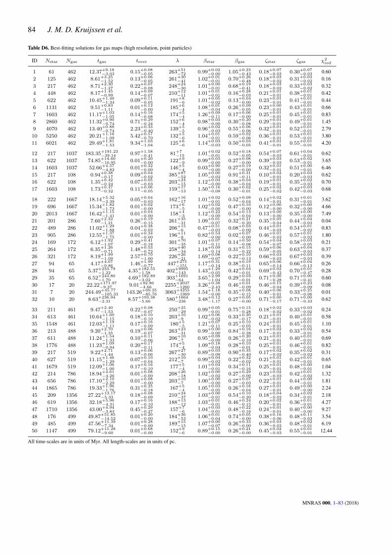
84 J. M. D. Kruijssen et al.
Table D6. Best-fitting solutions for gas maps (high resolution, point particles)
ID Nstar Ngas tgas tover λ βstar βgas ζstar ζgas χ2red
1 61 462 12.37+9.18−3.03 0.15+0.08
−0.05 263+51−72 0.99+0.02
−0.00 1.05+0.23−0.43 0.18+0.07
−0.03 0.30+0.07−0.03 0.60
2 125 462 8.61+3.25−1.52 0.13+0.06
−0.05 261+30−41 1.02+0.01
−0.01 0.70+0.26−0.48 0.18+0.03
−0.02 0.31+0.03−0.02 0.16
3 217 462 8.71+2.30−1.27 0.22+0.07
−0.08 248+24−30 1.01+0.00
−0.01 0.68+0.19−0.41 0.18+0.03
−0.02 0.33+0.03−0.02 0.32
4 448 462 8.17+1.45−0.99 0.14+0.09
−0.07 210+12−11 1.01+0.01
−0.01 0.16+0.28−0.03 0.21+0.01
−0.01 0.38+0.01−0.01 0.42
5 622 462 10.45+1.40−1.34 0.09+0.11
−0.05 191+8−6 1.01+0.05
−0.02 0.13+0.04−0.00 0.23+0.01
−0.01 0.41+0.01−0.01 0.44
6 1131 462 9.51+0.83−1.11 0.01+0.12
−0.00 185+6−4 1.08+0.01
−0.04 0.26+0.09−0.05 0.23+0.00
−0.01 0.43+0.01−0.01 0.66
7 1603 462 11.17+1.03−1.05 0.14+0.16
−0.08 174+5−4 1.26+0.09
−0.11 0.17+0.06−0.00 0.25+0.01
−0.01 0.45+0.01−0.01 0.83
8 2860 462 11.32+0.90−0.74 0.71+0.29
−0.24 152+6−4 0.98+0.03
−0.00 0.30+0.20−0.08 0.29+0.01
−0.01 0.49+0.01−0.01 1.45
9 4070 462 13.40+0.88−0.74 2.23+0.33
−0.40 139+5−5 0.96+0.02
−0.03 0.55+0.06−0.06 0.32+0.01
−0.01 0.52+0.01−0.01 2.79
10 5250 462 20.21+1.16−1.09 5.42+0.57
−0.70 132+5−6 1.04+0.01
−0.01 0.59+0.02−0.06 0.36+0.01
−0.01 0.53+0.01−0.01 3.80
11 6021 462 29.49+1.81−1.53 9.34+1.03
−1.04 125+6−6 1.14+0.03
−0.03 0.50+0.03−0.05 0.41+0.01
−0.01 0.55+0.01−0.01 4.20
12 217 1037 183.35+191.23−39.14 0.97+1.58
−0.41 81+7−15 1.01+0.02
−0.01 0.52+0.18−0.05 0.54+0.07
−0.03 0.61+0.04−0.01 0.62
13 622 1037 74.85+14.60−10.95 0.01+0.20
−0.00 122+9−9 0.99+0.03
−0.00 0.27+0.08−0.00 0.39+0.03
−0.03 0.53+0.02−0.01 3.65
14 1603 1037 52.66+4.57−4.82 0.01+0.32
−0.00 146+5−4 0.03+0.90
−0.00 0.27+0.19−0.00 0.32+0.01
−0.01 0.51+0.00−0.01 6.46
15 217 108 0.94+0.38−0.17 0.09+0.04
−0.02 385+87−52 1.05+0.00
−0.02 0.91+0.31−0.11 0.10+0.02
−0.01 0.20+0.03−0.03 0.62
16 622 108 1.35+0.42−0.24 0.07+0.05
−0.03 203+24−15 1.12+0.04
−0.00 0.38+0.04−0.04 0.19+0.01
−0.01 0.35+0.02−0.03 0.70
17 1603 108 1.73+0.47−0.32 0.11+0.06
−0.05 159+17−13 1.50+0.16
−0.08 0.30+0.02−0.01 0.25+0.02
−0.02 0.42+0.03−0.03 0.68
18 222 1667 18.14+5.32−3.39 0.05+0.04
−0.03 162+16−17 1.01+0.02
−0.01 0.52+0.09−0.04 0.14+0.02
−0.01 0.31+0.01−0.01 3.62
19 696 1667 15.34+1.82−1.73 0.01+0.02
−0.00 173+6−5 1.02+0.02
−0.00 0.47+0.10−0.00 0.12+0.00
−0.00 0.32+0.00−0.00 4.66
20 2013 1667 16.42+1.15−1.41 0.01+0.04
−0.00 158+4−3 1.12+0.22
−0.00 0.54+0.13−0.04 0.13+0.00
−0.00 0.35+0.00−0.00 7.49
21 201 286 7.60+2.32−1.21 0.26+0.19
−0.15 261+35−31 1.09+0.01
−0.07 0.32+0.21−0.20 0.35+0.05
−0.04 0.44+0.04−0.03 0.04
22 489 286 11.02+1.29−1.88 0.04+0.38
−0.02 206+15−6 0.47+0.51
−0.02 0.08+0.03−0.00 0.44+0.01
−0.03 0.54+0.01−0.02 0.83
23 905 286 12.55+1.37−1.75 0.01+0.34
−0.00 196+11−8 0.82+0.54
−0.00 0.02+0.07−0.00 0.46+0.01
−0.02 0.57+0.01−0.02 1.80
24 169 172 6.12+1.92−1.07 0.29+0.41
−0.18 301+70−35 1.01+0.07
−0.11 0.14+0.50−0.08 0.54+0.04
−0.07 0.58+0.03−0.05 0.21
25 264 172 6.35+1.26−0.71 1.48+0.53
−0.72 258+40−34 1.18+0.09
−0.14 0.31+0.15−0.22 0.59+0.06
−0.05 0.63+0.04−0.03 0.37
26 321 172 8.19+1.99−1.09 2.57+0.70
−1.00 226+26−21 1.69+0.08
−0.07 0.22+0.10−0.13 0.66+0.03
−0.03 0.67+0.03−0.03 0.39
27 94 65 4.17+4.07−0.86 1.46+1.99
−0.77 447+275−151 1.17+0.31
−0.14 0.38+0.19−0.11 0.65+0.06
−0.14 0.66+0.04−0.13 0.26
28 94 65 5.37+233.79−1.22 4.35+182.55
−1.58 402+9995−143 1.43+1.29
−0.05 0.42+0.04−0.01 0.69+0.02
−0.42 0.70+0.01−0.47 0.28
29 35 65 6.52+244.80−1.70 4.69+182.89
−3.02 303+1691−64 3.65+2.99
−1.04 0.29+0.03−0.01 0.71+0.00
−0.28 0.71+0.00−0.41 0.60
30 17 20 22.22+171.97−9.37 9.01+92.86
−4.66 2255+2037−1260 3.26+0.38
−2.43 0.46+0.01−0.09 0.46+0.15
−0.04 0.39+0.23−0.09 0.08
31 7 20 244.49+45.77−105.33 143.26+69.35
−85.76 3063+4255−1969 1.54+1.18
−0.00 0.35+0.08−0.15 0.40+0.06
−0.01 0.33+0.25−0.06 0.01
32 10 20 8.63+236.94−2.31 8.57+193.38
−5.60 580+1664−236 3.48+0.12
−1.17 0.27+0.05−0.00 0.71+0.00
−0.17 0.71+0.00−0.33 0.62
33 211 461 9.47+2.40−1.53 0.22+0.08
−0.07 250+25−29 0.99+0.05
−0.01 0.75+0.15−0.28 0.18+0.02
−0.02 0.33+0.03−0.02 0.24
34 613 461 10.64+1.60−1.15 0.18+0.10
−0.10 203+10−9 1.02+0.06
−0.02 0.33+0.20−0.17 0.21+0.01
−0.01 0.40+0.01−0.01 0.58
35 1548 461 12.03+1.19−1.11 0.17+0.16
−0.09 180+5−5 1.21+0.07
−0.11 0.25+0.10−0.05 0.24+0.01
−0.01 0.45+0.01−0.01 1.10
36 213 488 9.20+2.70−1.35 0.19+0.06
−0.07 263+23−31 0.99+0.00
−0.00 0.84+0.16−0.38 0.17+0.02
−0.01 0.33+0.02−0.01 0.54
37 611 488 11.24+1.54−1.33 0.10+0.11
−0.06 206+10−7 0.95+0.09
−0.00 0.26+0.20−0.10 0.21+0.01
−0.01 0.40+0.01−0.01 0.69
38 1776 488 11.23+1.09−0.94 0.20+0.17
−0.11 174+5−4 1.09+0.18
−0.04 0.28+0.10−0.01 0.25+0.01
−0.01 0.46+0.01−0.01 0.82
39 217 519 9.22+2.71−1.44 0.13+0.06
−0.06 267+27−30 0.89+0.03
−0.08 0.90+0.35−0.40 0.17+0.02
−0.02 0.35+0.02−0.02 0.31
40 627 519 11.15+1.46−1.29 0.07+0.10
−0.04 212+10−7 0.99+0.04
−0.02 0.22+0.32−0.02 0.21+0.01
−0.01 0.42+0.01−0.01 0.65
41 1679 519 12.09+1.06−1.00 0.17+0.16
−0.10 177+5−4 1.01+0.04
−0.01 0.34+0.11−0.16 0.25+0.01
−0.01 0.48+0.00−0.01 1.04
42 214 786 18.94+4.61−4.26 0.01+0.08
−0.00 208+26−18 1.02+0.00
−0.02 0.27+0.29−0.00 0.23+0.02
−0.03 0.42+0.01−0.02 1.32
43 656 786 17.10+2.10−2.29 0.01+0.08
−0.00 203+10−7 1.00+0.00
−0.00 0.27+0.07−0.03 0.22+0.01
−0.01 0.44+0.00−0.01 1.81
44 1865 786 19.33+1.96−1.76 0.31+0.25
−0.18 167+5−4 1.05+0.03
−0.05 0.26+0.16−0.04 0.27+0.01
−0.01 0.49+0.00−0.00 2.24
45 209 1356 27.22+13.17−5.33 0.18+0.08
−0.09 210+24−37 1.03+0.00
−0.01 0.54+0.10−0.20 0.18+0.04
−0.02 0.34+0.02−0.01 2.18
46 619 1356 32.18+5.96−4.31 0.17+0.16
−0.10 188+13−12 1.03+0.01
−0.01 0.46+0.24−0.15 0.20+0.02
−0.01 0.36+0.01−0.01 4.27
47 1710 1356 43.00+4.94−3.83 0.45+0.29
−0.27 157+7−6 1.04+0.03
−0.01 0.48+0.22−0.16 0.24+0.01
−0.01 0.40+0.00−0.00 9.27
48 176 499 49.87+51.85−14.52 0.01+0.20
−0.00 184+36−53 1.06+0.01
−0.04 0.74+0.05−0.00 0.38+0.16
−0.06 0.48+0.11−0.03 3.54
49 485 499 47.56+11.39−7.34 0.01+0.28
−0.00 189+15−15 1.07+0.00
−0.07 0.26+0.33−0.00 0.36+0.03
−0.03 0.48+0.02−0.01 6.19
50 1147 499 79.12+11.28−9.60 0.01+0.68
−0.00 152+9−6 0.89+0.15
−0.00 0.26+0.21−0.00 0.45+0.02
−0.03 0.55+0.01−0.01 12.44
All time-scales are in units of Myr. All length-scales are in units of pc.
MNRAS 000, 1–83 (2018)

Cloud-scale star formation across cosmic history 85
Table D7. Best-fitting solutions for gas maps (low resolution, extended emission)
ID Nstar Ngas tgas tover λ βstar βgas ζstar ζgas χ2red
1 15 137 27.21+653.94−9.80 1.01+27.84
−0.30 695+121−171 1.54+0.31
−0.22 1.31+0.18−0.11 0.46+0.08
−0.04 0.42+0.07−0.03 0.38
2 25 137 20.13+625.50−6.50 1.67+55.31
−0.44 878+184−247 1.25+1.79
−0.03 1.06+0.09−0.17 0.38+0.10
−0.05 0.37+0.08−0.04 0.50
3 42 169 12.72+3.99−2.51 1.25+0.51
−0.31 598+107−70 0.66+0.05
−0.02 1.03+0.11−0.09 0.40+0.03
−0.03 0.37+0.03−0.03 0.85
4 74 169 13.85+2.67−2.92 3.64+0.82
−0.87 610+117−101 0.87+0.04
−0.01 0.97+0.03−0.07 0.39+0.04
−0.03 0.38+0.05−0.04 1.25
5 86 169 10.92+2.76−1.35 2.87+1.13
−0.51 377+103−52 0.92+0.09
−0.02 0.83+0.08−0.12 0.52+0.02
−0.06 0.52+0.03−0.07 0.66
6 100 169 11.47+5.06−1.55 4.40+2.57
−0.87 329+112−45 0.99+0.01
−0.05 0.81+0.15−0.10 0.52+0.03
−0.05 0.55+0.03−0.07 0.37
7 108 169 16.14+6.10−2.19 6.40+3.07
−1.29 325+86−43 1.06+0.07
−0.07 0.62+0.09−0.05 0.55+0.02
−0.03 0.56+0.03−0.04 0.20
8 109 169 17.87+4.60−2.96 12.20+3.23
−2.23 339+88−52 0.96+0.10
−0.03 0.71+0.02−0.02 0.54+0.03
−0.03 0.56+0.03−0.05 0.30
9 114 169 21.59+6.21−2.75 18.26+4.69
−2.57 352+120−52 1.04+0.20
−0.08 0.59+0.05−0.02 0.53+0.03
−0.05 0.56+0.03−0.07 0.29
10 108 169 36.08+36.07−5.00 35.98+32.34
−5.82 376+352−68 1.08+0.14
−0.09 1.74+0.00−1.11 0.52+0.03
−0.11 0.55+0.03−0.17 0.90
11 85 169 66.92+37.49−9.73 66.15+30.82
−11.96 397+189−65 0.83+0.11
−0.04 0.68+0.05−0.13 0.51+0.03
−0.07 0.54+0.03−0.11 0.65
12 42 206 598.74+1452.38−210.80 28.35+73.57
−9.67 444+73−52 0.22+0.03
−0.07 1.59+0.02−0.09 0.50+0.03
−0.03 0.53+0.03−0.03 0.70
13 86 206 2608.31+222.74−872.57 301.92+37.24
−102.52 381+57−43 0.39+0.13
−0.10 1.30+0.03−0.03 0.56+0.02
−0.03 0.56+0.02−0.03 0.94
14 108 206 1022.09+1303.32−280.18 143.67+181.92
−43.61 350+56−54 1.09+1.23
−0.52 1.30+0.06−0.02 0.58+0.02
−0.02 0.57+0.03−0.02 0.58
15 42 64 1.22+0.63−0.30 0.20+0.13
−0.12 666+194−143 0.93+0.02
−0.01 0.45+0.24−0.26 0.34+0.05
−0.05 0.29+0.06−0.05 0.46
16 86 64 0.84+0.36−0.18 0.56+0.16
−0.11 274+88−48 1.36+0.08
−0.10 1.28+0.20−0.42 0.56+0.04
−0.05 0.54+0.06−0.07 0.24
17 108 64 1.44+0.76−0.25 1.38+0.31
−0.29 262+98−43 2.08+0.09
−0.01 1.18+0.10−0.42 0.57+0.03
−0.05 0.55+0.05−0.08 0.20
18 42 169 12.72+3.96−2.52 1.25+0.51
−0.31 598+109−70 0.66+0.05
−0.02 1.03+0.11−0.09 0.40+0.03
−0.03 0.37+0.03−0.03 0.85
19 88 198 10.25+2.35−1.05 2.68+0.92
−0.38 346+83−43 0.85+0.00
−0.03 0.75+0.12−0.13 0.47+0.02
−0.03 0.48+0.03−0.04 0.99
20 116 198 20.01+4.68−3.76 8.72+2.55
−2.16 345+65−49 0.77+0.07
−0.02 0.67+0.06−0.06 0.45+0.02
−0.02 0.49+0.03−0.03 0.38
21 42 169 12.72+3.98−2.51 1.25+0.51
−0.31 591+109−66 0.66+0.05
−0.02 1.03+0.11−0.09 0.41+0.03
−0.03 0.38+0.03−0.03 0.85
22 88 198 10.25+2.35−1.05 2.68+0.92
−0.38 348+83−43 0.85+0.00
−0.03 0.75+0.12−0.13 0.46+0.02
−0.03 0.48+0.03−0.04 0.97
23 116 198 20.01+4.69−3.76 8.72+2.55
−2.16 345+66−49 0.77+0.07
−0.02 0.67+0.06−0.05 0.45+0.02
−0.02 0.49+0.03−0.03 0.39
24 40 137 11.86+4.19−2.11 1.49+0.71
−0.32 699+227−120 1.04+0.32
−0.11 1.00+0.18−0.17 0.46+0.05
−0.08 0.43+0.05−0.06 0.33
25 80 137 12.21+3.39−1.85 4.29+1.62
−1.01 519+169−108 1.28+0.06
−0.10 0.90+0.11−0.13 0.54+0.07
−0.07 0.52+0.07−0.07 0.58
26 95 137 17.70+4.29−2.57 8.26+2.96
−1.67 381+116−63 1.11+0.17
−0.08 0.58+0.04−0.06 0.63+0.02
−0.06 0.61+0.03−0.07 0.24
27 35 84 13.81+626.59−3.13 2.59+130.64
−0.71 850+314−206 1.32+1.12
−0.14 0.90+0.27−0.12 0.52+0.08
−0.09 0.51+0.07−0.09 0.26
28 65 84 15.49+6.21−2.89 5.80+3.24
−1.68 597+380−142 1.22+0.28
−0.14 1.04+0.11−0.06 0.61+0.06
−0.11 0.61+0.07−0.12 0.60
29 71 84 17.25+5.06−2.93 9.70+3.54
−2.62 461+213−106 1.46+0.30
−0.17 0.64+0.07−0.06 0.67+0.03
−0.06 0.67+0.04−0.07 0.43
30 30 35 13.03+641.06−4.81 4.27+211.70
−1.55 1324+814−574 1.18+6.36
−0.16 1.04+0.47−0.41 0.54+0.17
−0.13 0.56+0.15−0.12 0.20
31 44 35 21.18+692.71−4.90 12.67+442.59
−5.14 1058+5997−495 1.87+4.25
−0.34 0.69+0.42−0.09 0.62+0.09
−0.33 0.62+0.09−0.34 0.49
32 37 35 25.26+713.28−5.54 16.33+539.97
−9.51 685+7399−328 2.09+6.93
−0.93 0.60+0.10−0.04 0.71+0.00
−0.43 0.71+0.00−0.47 0.71
33 40 172 11.82+4.95−2.08 1.11+0.64
−0.29 568+101−67 0.70+0.07
−0.01 0.85+0.19−0.07 0.43+0.03
−0.03 0.41+0.03−0.04 0.90
34 78 172 9.01+2.41−1.07 3.02+1.15
−0.47 352+126−48 0.79+0.09
−0.02 0.91+0.09−0.04 0.53+0.02
−0.06 0.55+0.03−0.07 0.32
35 98 172 16.50+4.26−2.35 8.45+2.81
−1.71 340+94−50 0.86+0.11
−0.02 0.65+0.04−0.02 0.52+0.03
−0.04 0.57+0.03−0.05 0.11
36 40 153 11.56+4.31−2.07 1.51+0.69
−0.32 634+136−70 0.73+0.06
−0.04 0.96+0.15−0.05 0.43+0.02
−0.03 0.40+0.03−0.04 1.12
37 70 153 9.24+3.57−1.15 3.19+1.73
−0.54 345+129−48 0.76+0.04
−0.02 0.89+0.13−0.09 0.52+0.03
−0.05 0.57+0.02−0.07 0.40
38 84 153 15.90+4.77−2.19 9.75+3.38
−1.84 332+94−48 0.77+0.09
−0.03 0.66+0.04−0.01 0.52+0.03
−0.04 0.58+0.02−0.05 0.10
39 37 139 13.62+4.52−2.76 2.32+0.93
−0.60 642+142−83 0.52+0.05
−0.02 0.84+0.07−0.03 0.46+0.03
−0.03 0.42+0.03−0.04 0.72
40 66 139 9.98+3.24−1.23 4.27+1.93
−0.69 350+147−55 0.57+0.07
−0.03 0.83+0.07−0.13 0.52+0.03
−0.06 0.58+0.02−0.08 0.30
41 76 139 15.25+7.47−2.55 11.30+5.77
−2.22 356+164−57 0.78+0.05
−0.01 0.82+0.17−0.11 0.51+0.03
−0.05 0.59+0.02−0.09 0.14
42 35 90 10.25+6.04−2.36 1.76+1.38
−0.53 804+263−136 0.64+0.10
−0.01 1.05+0.14−0.08 0.48+0.04
−0.06 0.45+0.04−0.08 0.46
43 49 120 9.26+1.82−1.18 4.00+1.20
−0.65 400+133−61 0.64+0.07
−0.01 0.90+0.06−0.12 0.52+0.03
−0.06 0.58+0.02−0.07 0.35
44 61 120 16.49+10.73−2.87 14.10+8.81
−2.63 435+185−66 0.67+0.05
−0.07 1.06+0.40−0.27 0.46+0.02
−0.03 0.57+0.03−0.08 0.37
45 32 78 6.10+2.29−1.13 1.35+0.81
−0.41 849+315−169 0.50+0.17
−0.07 0.72+0.20−0.10 0.47+0.05
−0.06 0.51+0.05−0.08 0.27
46 35 78 7.09+1.93−1.02 3.97+1.38
−0.71 579+236−96 0.75+0.03
−0.01 0.96+0.41−0.06 0.53+0.04
−0.06 0.60+0.03−0.06 0.12
47 34 82 18.08+4.17−3.06 15.56+3.14
−3.06 573+145−98 0.65+0.04
−0.01 1.27+0.51−0.32 0.45+0.04
−0.04 0.57+0.03−0.03 0.18
48 19 33 11.19+675.54−3.34 3.57+290.54
−1.50 940+1310−320 0.37+9.10
−0.06 0.82+0.10−0.08 0.58+0.07
−0.18 0.60+0.06−0.21 0.15
49 20 41 8.70+5.29−1.59 4.86+3.75
−0.91 632+294−127 0.84+0.08
−0.26 0.92+0.07−0.11 0.57+0.03
−0.07 0.64+0.02−0.05 0.18
50 15 41 39.00+32.87−8.42 38.18+23.76
−9.98 776+411−249 0.37+0.06
−0.03 0.73+0.10−0.02 0.44+0.09
−0.04 0.61+0.03−0.08 0.21
All time-scales are in units of Myr. All length-scales are in units of pc.
MNRAS 000, 1–83 (2018)

86 J. M. D. Kruijssen et al.
Table D8. Best-fitting solutions for gas maps (high resolution, extended emission)
ID Nstar Ngas tgas tover λ βstar βgas ζstar ζgas χ2red
1 58 293 6.95+2.13−1.39 0.31+0.11
−0.06 374+73−54 1.13+0.16
−0.14 0.80+0.12−0.10 0.33+0.04
−0.05 0.29+0.03−0.03 0.21
2 109 293 3.93+0.87−0.49 0.27+0.09
−0.09 339+46−55 1.31+0.02
−0.16 0.60+0.13−0.23 0.34+0.04
−0.03 0.33+0.04−0.03 0.38
3 180 293 3.38+0.51−0.40 0.39+0.09
−0.12 295+40−40 1.08+0.09
−0.08 0.57+0.12−0.16 0.37+0.04
−0.03 0.37+0.04−0.03 0.61
4 297 293 3.21+0.42−0.27 0.52+0.12
−0.18 212+24−23 1.01+0.12
−0.12 0.38+0.12−0.16 0.47+0.03
−0.03 0.49+0.03−0.03 0.33
5 353 293 3.64+0.49−0.30 0.74+0.10
−0.15 174+15−14 1.17+0.20
−0.12 0.32+0.11−0.04 0.52+0.02
−0.01 0.54+0.02−0.01 0.37
6 414 293 2.76+0.33−0.18 1.07+0.12
−0.09 137+13−9 1.41+0.03
−0.19 0.46+0.08−0.05 0.58+0.01
−0.02 0.59+0.01−0.02 0.20
7 409 293 3.99+0.48−0.40 1.96+0.15
−0.23 140+12−10 1.43+0.07
−0.01 0.54+0.04−0.05 0.58+0.01
−0.01 0.59+0.01−0.01 0.32
8 351 293 5.84+0.78−0.58 4.11+0.33
−0.40 144+15−12 1.39+0.12
−0.08 0.49+0.06−0.03 0.57+0.02
−0.02 0.59+0.02−0.02 0.29
9 274 293 6.99+1.18−0.42 6.96+0.89
−0.51 136+19−9 1.45+0.01
−0.03 0.46+0.17−0.00 0.60+0.01
−0.02 0.60+0.01−0.02 1.59
10 239 293 14.48+2.90−1.07 14.46+2.38
−1.24 150+25−12 1.26+0.01
−0.04 0.70+0.00−0.22 0.60+0.01
−0.02 0.58+0.02−0.03 0.63
11 170 293 21.31+2.27−1.82 21.31+1.98
−2.05 145+15−13 1.51+0.01
−0.00 0.38+0.12−0.00 0.60+0.01
−0.01 0.59+0.02−0.02 2.99
12 180 371 36.17+11.18−5.75 2.37+0.84
−0.38 218+21−18 0.86+0.02
−0.01 1.03+0.02−0.01 0.49+0.03
−0.03 0.50+0.02−0.02 0.80
13 353 371 33.33+3.81−3.28 4.11+0.64
−0.57 183+11−11 0.88+0.04
−0.01 0.75+0.04−0.08 0.55+0.01
−0.01 0.55+0.01−0.01 0.95
14 409 371 28.50+2.42−1.91 5.75+0.74
−0.78 170+11−11 1.02+0.05
−0.01 0.73+0.02−0.01 0.57+0.01
−0.01 0.58+0.01−0.01 1.11
15 180 94 0.25+0.13−0.05 0.06+0.05
−0.03 223+105−40 1.17+0.23
−0.12 0.61+0.22−0.29 0.41+0.06
−0.10 0.40+0.06−0.12 0.46
16 353 94 0.20+0.12−0.04 0.11+0.03
−0.02 98+34−13 2.90+0.24
−0.05 0.56+0.10−0.22 0.64+0.01
−0.07 0.63+0.02−0.08 0.33
17 409 94 0.39+3.25−0.01 0.39+1.82
−0.01 93+743−8 1.93+0.75
−0.38 0.88+0.16−0.34 0.65+0.01
−0.36 0.63+0.01−0.49 1.17
18 180 293 3.38+0.51−0.40 0.39+0.09
−0.12 295+39−40 1.08+0.09
−0.08 0.57+0.12−0.16 0.37+0.04
−0.03 0.37+0.04−0.03 0.61
19 361 316 3.50+0.33−0.29 0.62+0.07
−0.11 165+12−12 0.95+0.05
−0.05 0.43+0.02−0.08 0.48+0.01
−0.01 0.51+0.01−0.01 0.40
20 467 316 3.49+0.37−0.26 1.70+0.15
−0.09 127+10−7 1.31+0.03
−0.05 0.61+0.03−0.02 0.54+0.01
−0.01 0.57+0.01−0.02 0.29
21 171 251 4.21+0.75−0.57 0.42+0.14
−0.20 320+45−54 1.21+0.14
−0.25 0.56+0.07−0.38 0.43+0.06
−0.03 0.43+0.05−0.03 0.47
22 294 251 4.06+0.66−0.39 0.87+0.28
−0.29 197+23−18 1.30+0.03
−0.11 0.27+0.13−0.14 0.59+0.02
−0.04 0.60+0.01−0.03 0.25
23 298 251 4.19+0.72−0.51 1.95+0.24
−0.25 150+16−12 1.98+0.03
−0.06 0.41+0.02−0.12 0.64+0.01
−0.01 0.65+0.01−0.01 0.43
24 157 159 4.11+0.95−0.67 0.58+0.30
−0.28 349+72−58 1.13+0.16
−0.05 0.47+0.04−0.35 0.55+0.05
−0.06 0.56+0.04−0.05 0.12
25 198 159 3.66+0.57−0.44 2.17+0.45
−0.43 251+53−38 1.28+0.06
−0.03 0.55+0.03−0.09 0.64+0.05
−0.05 0.65+0.04−0.04 0.37
26 151 159 5.17+0.92−0.59 3.96+0.65
−0.53 213+38−25 1.76+0.06
−0.08 0.55+0.05−0.16 0.69+0.02
−0.03 0.69+0.02−0.04 0.52
27 90 63 3.66+3.56−0.71 1.44+2.22
−0.74 476+446−163 1.30+0.21
−0.15 0.43+0.16−0.24 0.63+0.07
−0.17 0.65+0.06−0.16 0.28
28 81 63 4.83+231.65−1.17 4.35+183.22
−1.37 418+8529−141 1.46+1.61
−0.02 0.80+0.08−0.37 0.67+0.03
−0.40 0.69+0.02−0.46 0.21
29 22 63 5.46+246.66−1.25 5.18+194.68
−3.10 300+2109−67 3.43+1.00
−0.97 0.51+0.02−0.22 0.71+0.00
−0.31 0.71+0.00−0.43 0.55
30 17 20 64.46+132.87−28.57 26.60+80.29
−13.42 2212+2111−1248 1.63+1.18
−0.84 0.47+0.01−0.09 0.47+0.16
−0.05 0.39+0.23−0.09 0.07
31 7 20 309.14+0.00−135.03 175.19+56.84
−121.53 3065+7254−1956 1.56+1.18
−0.00 0.34+0.07−0.16 0.41+0.06
−0.01 0.33+0.24−0.08 0.00
32 10 20 7.76+238.08−2.02 7.75+192.65
−5.06 532+1719−210 3.65+0.66
−1.32 0.27+0.05−0.00 0.71+0.00
−0.16 0.71+0.00−0.34 0.65
33 166 281 3.37+0.47−0.42 0.43+0.08
−0.12 311+36−42 1.04+0.03
−0.08 0.65+0.04−0.16 0.37+0.04
−0.02 0.37+0.04−0.02 0.61
34 318 281 3.38+0.40−0.30 0.77+0.16
−0.13 177+19−15 1.30+0.02
−0.03 0.38+0.05−0.11 0.54+0.01
−0.02 0.54+0.02−0.02 0.27
35 329 281 4.06+0.50−0.45 2.23+0.03
−0.28 144+10−12 1.44+0.08
−0.01 0.52+0.04−0.04 0.58+0.01
−0.01 0.59+0.02−0.01 0.13
36 162 254 3.07+0.47−0.33 0.46+0.10
−0.10 333+46−45 1.06+0.06
−0.07 0.62+0.08−0.13 0.38+0.03
−0.03 0.38+0.04−0.03 0.41
37 281 254 2.86+0.35−0.23 0.93+0.17
−0.10 185+21−16 1.34+0.00
−0.05 0.49+0.03−0.06 0.54+0.01
−0.02 0.56+0.01−0.02 0.19
38 259 254 3.76+0.43−0.39 2.52+0.09
−0.20 150+12−13 1.52+0.01
−0.03 0.64+0.02−0.10 0.59+0.01
−0.01 0.60+0.01−0.01 0.12
39 152 235 2.68+0.36−0.33 0.41+0.08
−0.09 326+43−42 1.19+0.09
−0.10 0.64+0.07−0.12 0.41+0.03
−0.02 0.42+0.03−0.02 0.45
40 236 235 2.72+0.36−0.24 1.02+0.20
−0.13 193+26−18 1.39+0.01
−0.03 0.52+0.07−0.04 0.56+0.01
−0.03 0.58+0.01−0.03 0.22
41 196 235 3.18+0.44−0.17 2.90+0.03
−0.05 148+14−11 1.76+0.12
−0.24 0.56+0.05−0.02 0.60+0.01
−0.01 0.62+0.01−0.01 0.16
42 126 164 2.32+0.50−0.27 0.47+0.13
−0.12 357+53−55 1.35+0.06
−0.23 0.52+0.04−0.04 0.48+0.04
−0.03 0.51+0.03−0.03 0.41
43 183 187 2.83+0.26−0.25 1.44+0.14
−0.16 221+31−24 1.07+0.16
−0.03 0.56+0.02−0.04 0.54+0.03
−0.03 0.57+0.03−0.03 0.17
44 139 187 4.11+0.36−0.19 4.10+0.23
−0.26 186+22−14 1.31+0.02
−0.00 0.58+0.08−0.07 0.58+0.01
−0.02 0.61+0.01−0.02 0.45
45 97 121 1.81+0.35−0.23 0.45+0.12
−0.13 365+52−50 1.10+0.03
−0.06 0.42+0.06−0.03 0.52+0.03
−0.03 0.56+0.02−0.02 0.44
46 96 138 2.13+0.29−0.21 1.43+0.20
−0.16 227+34−23 1.39+0.06
−0.02 0.48+0.01−0.02 0.56+0.02
−0.02 0.61+0.02−0.02 0.25
47 58 138 4.37+0.71−0.18 4.37+0.65
−0.24 203+36−18 1.36+0.00
−0.04 0.81+0.00−0.27 0.54+0.01
−0.02 0.63+0.01−0.03 1.16
48 41 45 1.20+0.22−0.15 0.67+0.08
−0.12 440+106−94 1.24+0.32
−0.26 0.50+0.07−0.05 0.57+0.05
−0.05 0.63+0.03−0.03 0.28
49 37 48 3.04+0.61−0.33 2.52+0.53
−0.26 336+79−51 1.42+0.04
−0.11 0.55+0.02−0.07 0.58+0.02
−0.03 0.62+0.02−0.03 0.12
50 23 48 22.36+5.34−5.88 22.01+5.15
−5.56 1456+67−186 2.14+0.06
−0.14 0.20+0.06−0.00 0.44+0.02
−0.01 0.36+0.03−0.01 4.31
All time-scales are in units of Myr. All length-scales are in units of pc.
MNRAS 000, 1–83 (2018)