an overview of the coding standard mpeg-4 audio … · eurasip journal on audio, speech, ... 2dolby...

Hindawi Publishing CorporationEURASIP Journal on Audio, Speech, and Music ProcessingVolume 2009, Article ID 468971, 21 pagesdoi:10.1155/2009/468971

Review Article

An Overview of the Coding Standard MPEG-4 AudioAmendments 1 and 2: HE-AAC, SSC, and HE-AAC v2

A. C. den Brinker,1 J. Breebaart,1 P. Ekstrand,2 J. Engdegard,2 F. Henn,2 K. Kjorling,2

W. Oomen,3 and H. Purnhagen2

1 Philips Research Laboratories, High Tech Campus 36, 5656 AE Eindhoven, The Netherlands2 Dolby Sweden AB, Gavlegatan 12 A, 11330 Stockholm, Sweden3 Philips Applied Technologies Eindhoven, High Tech Campus 5, 5656 AE Eindhoven, The Netherlands

Correspondence should be addressed to A. C. den Brinker, [email protected]

Received 29 September 2008; Accepted 24 February 2009

Recommended by James Kates

In 2003 and 2004, the ISO/IEC MPEG standardization committee added two amendments to their MPEG-4 audio coding standard.These amendments concern parametric coding techniques and encompass Spectral Band Replication (SBR), Sinusoidal Coding(SSC), and Parametric Stereo (PS). In this paper, we will give an overview of the basic ideas behind these techniques and referencesto more detailed information. Furthermore, the results of listening tests as performed during the final stages of the MPEG-4standardization process are presented in order to illustrate the performance of these techniques.

Copyright © 2009 A. C. den Brinker et al. This is an open access article distributed under the Creative Commons AttributionLicense, which permits unrestricted use, distribution, and reproduction in any medium, provided the original work is properlycited.

1. Introduction

The MPEG-2 Audio coding standard was released in 1997and has successfully found its way into the market. Later,MPEG-4 Audio Version 1 and Version 2 were issued inmid 1999 and early 2000, respectively. These versions haveadopted the MPEG-2 AAC coder including several exten-sions to it. In addition several other components like speechcoders (HVXC and CELP) and a Text-To-Speech Interfaceare specified.

In 2001, MPEG identified two areas for improved audiocoding technology and issued a Call for Proposals (CfP, [1]).These two areas were

(i) improved compression efficiency of audio signalsor speech signals by means of bandwidth extensionwhich is forward and backward compatible withexisting MPEG-4 technology;

(ii) improved compression efficiency of high-qualityaudio signals by means of parametric coding.

This started a new cycle in the standardization process,consisting of a competitive phase leading to a selection ofthe reference model, a collaborative phase for improving the

technology and, finally, the definition of a new standard.Close to the finalization of the work on parametric coding,it was demonstrated that the parametric stereo (PS) modulethat was developed in the course of the this work item couldalso be combined with the bandwidth extension technologythereby providing a significant additional boost in codingefficiency. This particular combination was subsequentlyadded to the parametric coding amendment. The work onbandwidth extension and parametric coding reached thefinal stage of Amendment 1 and 2 to MPEG-4 Audio mid2003 and 2004, respectively.

This paper has the intention to outline the ingredients ofthe MPEG-4 Audio Amendments in a comprehensive way.Part of this material is present in the literature but mostlyscattered. Therefore, this paper sets out to give an overview ofthe three components that make up these Amendments withreferences to more detailed information where necessary.

The outline of the paper is as follows. The basictechnology and subjective test results for the bandwidthextension and parametric coding are discussed in Sections 2and 3, respectively. In Section 4, the combination of AAC,SBR and PS is outlined, including subjective test results.Finally, in Section 5, the conclusions are presented.

2 EURASIP Journal on Audio, Speech, and Music Processing

Audio

input

SBRencoder

SBR data

Filteredaudiodata

Coreencoder

Bitmux

Bitstream

SBR data

Bitde

mux

Coredecoder

Audio

dataSBR

decoder

Audio

output

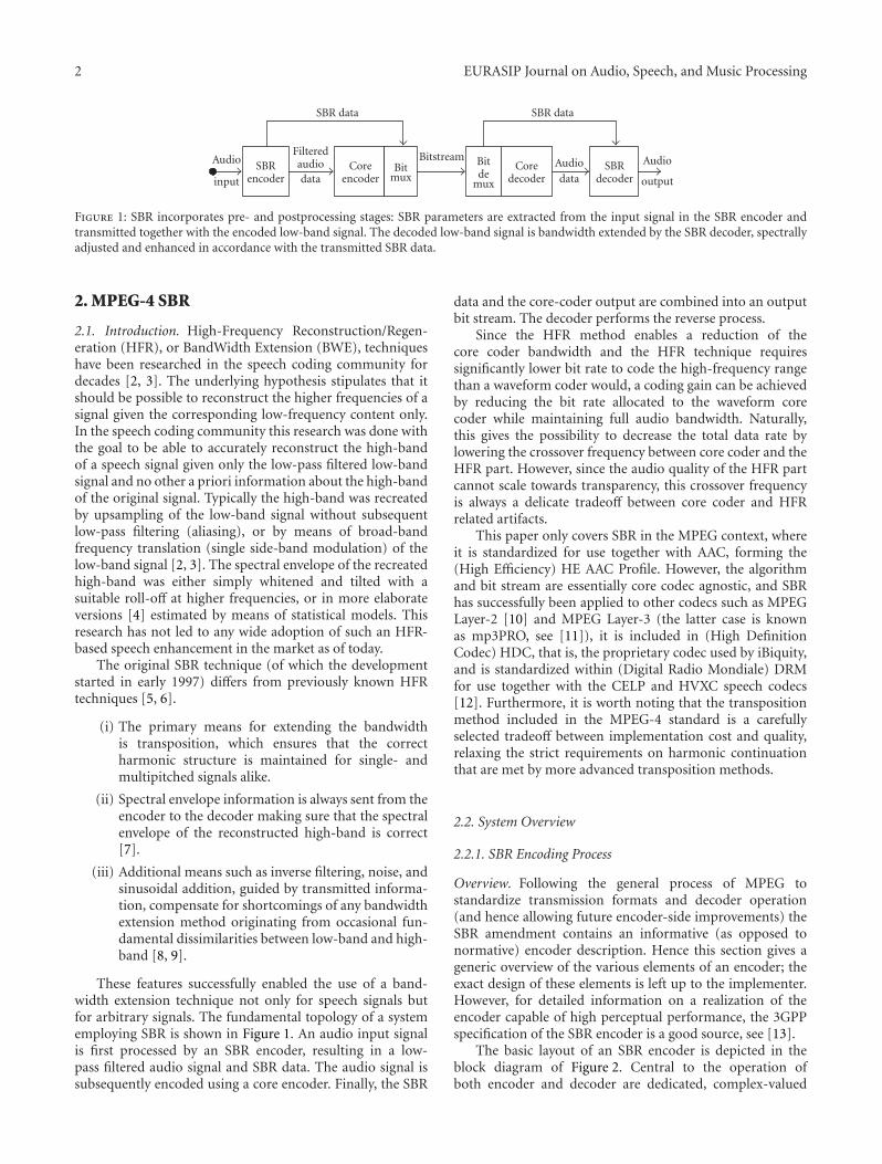
Figure 1: SBR incorporates pre- and postprocessing stages: SBR parameters are extracted from the input signal in the SBR encoder andtransmitted together with the encoded low-band signal. The decoded low-band signal is bandwidth extended by the SBR decoder, spectrallyadjusted and enhanced in accordance with the transmitted SBR data.

2. MPEG-4 SBR

2.1. Introduction. High-Frequency Reconstruction/Regen-eration (HFR), or BandWidth Extension (BWE), techniqueshave been researched in the speech coding community fordecades [2, 3]. The underlying hypothesis stipulates that itshould be possible to reconstruct the higher frequencies of asignal given the corresponding low-frequency content only.In the speech coding community this research was done withthe goal to be able to accurately reconstruct the high-bandof a speech signal given only the low-pass filtered low-bandsignal and no other a priori information about the high-bandof the original signal. Typically the high-band was recreatedby upsampling of the low-band signal without subsequentlow-pass filtering (aliasing), or by means of broad-bandfrequency translation (single side-band modulation) of thelow-band signal [2, 3]. The spectral envelope of the recreatedhigh-band was either simply whitened and tilted with asuitable roll-off at higher frequencies, or in more elaborateversions [4] estimated by means of statistical models. Thisresearch has not led to any wide adoption of such an HFR-based speech enhancement in the market as of today.

The original SBR technique (of which the developmentstarted in early 1997) differs from previously known HFRtechniques [5, 6].

(i) The primary means for extending the bandwidthis transposition, which ensures that the correctharmonic structure is maintained for single- andmultipitched signals alike.

(ii) Spectral envelope information is always sent from theencoder to the decoder making sure that the spectralenvelope of the reconstructed high-band is correct[7].

(iii) Additional means such as inverse filtering, noise, andsinusoidal addition, guided by transmitted informa-tion, compensate for shortcomings of any bandwidthextension method originating from occasional fun-damental dissimilarities between low-band and high-band [8, 9].

These features successfully enabled the use of a band-width extension technique not only for speech signals butfor arbitrary signals. The fundamental topology of a systememploying SBR is shown in Figure 1. An audio input signalis first processed by an SBR encoder, resulting in a low-pass filtered audio signal and SBR data. The audio signal issubsequently encoded using a core encoder. Finally, the SBR

data and the core-coder output are combined into an outputbit stream. The decoder performs the reverse process.

Since the HFR method enables a reduction of thecore coder bandwidth and the HFR technique requiressignificantly lower bit rate to code the high-frequency rangethan a waveform coder would, a coding gain can be achievedby reducing the bit rate allocated to the waveform corecoder while maintaining full audio bandwidth. Naturally,this gives the possibility to decrease the total data rate bylowering the crossover frequency between core coder and theHFR part. However, since the audio quality of the HFR partcannot scale towards transparency, this crossover frequencyis always a delicate tradeoff between core coder and HFRrelated artifacts.

This paper only covers SBR in the MPEG context, whereit is standardized for use together with AAC, forming the(High Efficiency) HE AAC Profile. However, the algorithmand bit stream are essentially core codec agnostic, and SBRhas successfully been applied to other codecs such as MPEGLayer-2 [10] and MPEG Layer-3 (the latter case is knownas mp3PRO, see [11]), it is included in (High DefinitionCodec) HDC, that is, the proprietary codec used by iBiquity,and is standardized within (Digital Radio Mondiale) DRMfor use together with the CELP and HVXC speech codecs[12]. Furthermore, it is worth noting that the transpositionmethod included in the MPEG-4 standard is a carefullyselected tradeoff between implementation cost and quality,relaxing the strict requirements on harmonic continuationthat are met by more advanced transposition methods.

2.2. System Overview

2.2.1. SBR Encoding Process

Overview. Following the general process of MPEG tostandardize transmission formats and decoder operation(and hence allowing future encoder-side improvements) theSBR amendment contains an informative (as opposed tonormative) encoder description. Hence this section gives ageneric overview of the various elements of an encoder; theexact design of these elements is left up to the implementer.However, for detailed information on a realization of theencoder capable of high perceptual performance, the 3GPPspecification of the SBR encoder is a good source, see [13].

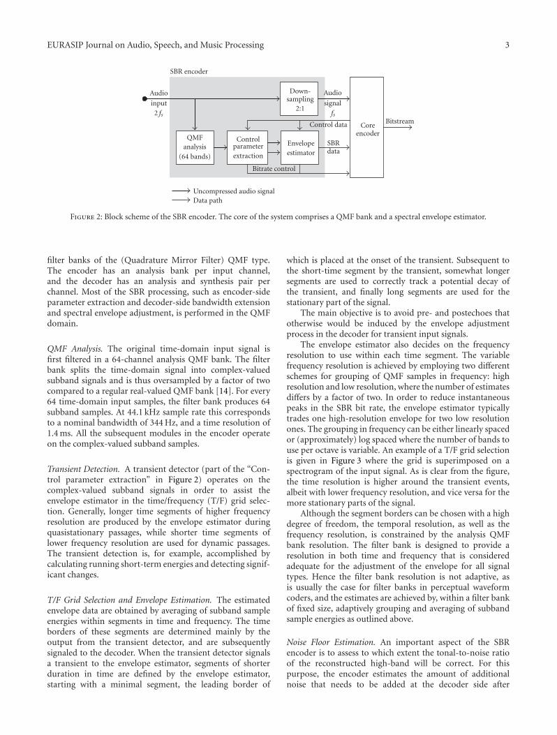
The basic layout of an SBR encoder is depicted in theblock diagram of Figure 2. Central to the operation ofboth encoder and decoder are dedicated, complex-valued

EURASIP Journal on Audio, Speech, and Music Processing 3

SBR encoder

Audio

input2 fs

Down-sampling

2:1

Audio

signal

fs

QMFanalysis

(64 bands)

Controlparameterextraction

Envelopeestimator

Bitrate control

Control data

SBRdata

Coreencoder

Bitstream

Uncompressed audio signalData path

Figure 2: Block scheme of the SBR encoder. The core of the system comprises a QMF bank and a spectral envelope estimator.

filter banks of the (Quadrature Mirror Filter) QMF type.The encoder has an analysis bank per input channel,and the decoder has an analysis and synthesis pair perchannel. Most of the SBR processing, such as encoder-sideparameter extraction and decoder-side bandwidth extensionand spectral envelope adjustment, is performed in the QMFdomain.

QMF Analysis. The original time-domain input signal isfirst filtered in a 64-channel analysis QMF bank. The filterbank splits the time-domain signal into complex-valuedsubband signals and is thus oversampled by a factor of twocompared to a regular real-valued QMF bank [14]. For every64 time-domain input samples, the filter bank produces 64subband samples. At 44.1 kHz sample rate this correspondsto a nominal bandwidth of 344 Hz, and a time resolution of1.4 ms. All the subsequent modules in the encoder operateon the complex-valued subband samples.

Transient Detection. A transient detector (part of the “Con-trol parameter extraction” in Figure 2) operates on thecomplex-valued subband signals in order to assist theenvelope estimator in the time/frequency (T/F) grid selec-tion. Generally, longer time segments of higher frequencyresolution are produced by the envelope estimator duringquasistationary passages, while shorter time segments oflower frequency resolution are used for dynamic passages.The transient detection is, for example, accomplished bycalculating running short-term energies and detecting signif-icant changes.

T/F Grid Selection and Envelope Estimation. The estimatedenvelope data are obtained by averaging of subband sampleenergies within segments in time and frequency. The timeborders of these segments are determined mainly by theoutput from the transient detector, and are subsequentlysignaled to the decoder. When the transient detector signalsa transient to the envelope estimator, segments of shorterduration in time are defined by the envelope estimator,starting with a minimal segment, the leading border of

which is placed at the onset of the transient. Subsequent tothe short-time segment by the transient, somewhat longersegments are used to correctly track a potential decay ofthe transient, and finally long segments are used for thestationary part of the signal.

The main objective is to avoid pre- and postechoes thatotherwise would be induced by the envelope adjustmentprocess in the decoder for transient input signals.

The envelope estimator also decides on the frequencyresolution to use within each time segment. The variablefrequency resolution is achieved by employing two differentschemes for grouping of QMF samples in frequency: highresolution and low resolution, where the number of estimatesdiffers by a factor of two. In order to reduce instantaneouspeaks in the SBR bit rate, the envelope estimator typicallytrades one high-resolution envelope for two low resolutionones. The grouping in frequency can be either linearly spacedor (approximately) log spaced where the number of bands touse per octave is variable. An example of a T/F grid selectionis given in Figure 3 where the grid is superimposed on aspectrogram of the input signal. As is clear from the figure,the time resolution is higher around the transient events,albeit with lower frequency resolution, and vice versa for themore stationary parts of the signal.

Although the segment borders can be chosen with a highdegree of freedom, the temporal resolution, as well as thefrequency resolution, is constrained by the analysis QMFbank resolution. The filter bank is designed to provide aresolution in both time and frequency that is consideredadequate for the adjustment of the envelope for all signaltypes. Hence the filter bank resolution is not adaptive, asis usually the case for filter banks in perceptual waveformcoders, and the estimates are achieved by, within a filter bankof fixed size, adaptively grouping and averaging of subbandsample energies as outlined above.

Noise Floor Estimation. An important aspect of the SBRencoder is to assess to which extent the tonal-to-noise ratioof the reconstructed high-band will be correct. For thispurpose, the encoder estimates the amount of additionalnoise that needs to be added at the decoder side after


regeneration of the high-band. This is done in an analysis-by-synthesis fashion. In Figure 4 such an analysis-by-synthesisprocess is illustrated. In the top panel of the figure a spectrumof the input signal is given. In this particular example theinput signal is a synthetically generated test signal of whichthe tonal (harmonic) structure ends abruptly above 5.5 kHz.The remaining spectrum of the signal consists of noise.In the lower panel of the figure a spectrum is given ofthe high-band given the HF generation method used inthe decoder, without additional correction of tonal-to-noiseproperties. In this case, the tonal structure of the low-bandhas propagated to the high-band (the region from 5.5 kHzto 15 kHz) and hence within the region of 5.5 to 15 kHz,there is a mismatch in signal characteristics between originalinput and reconstructed high-band signal. The transmissionof additional noise information allows correction of suchmismatches. It should be noted that the spectrum in thelower panel illustrates the low-band signal in combinationwith the high-band signal after HF generation without anysubsequent envelope adjustment.

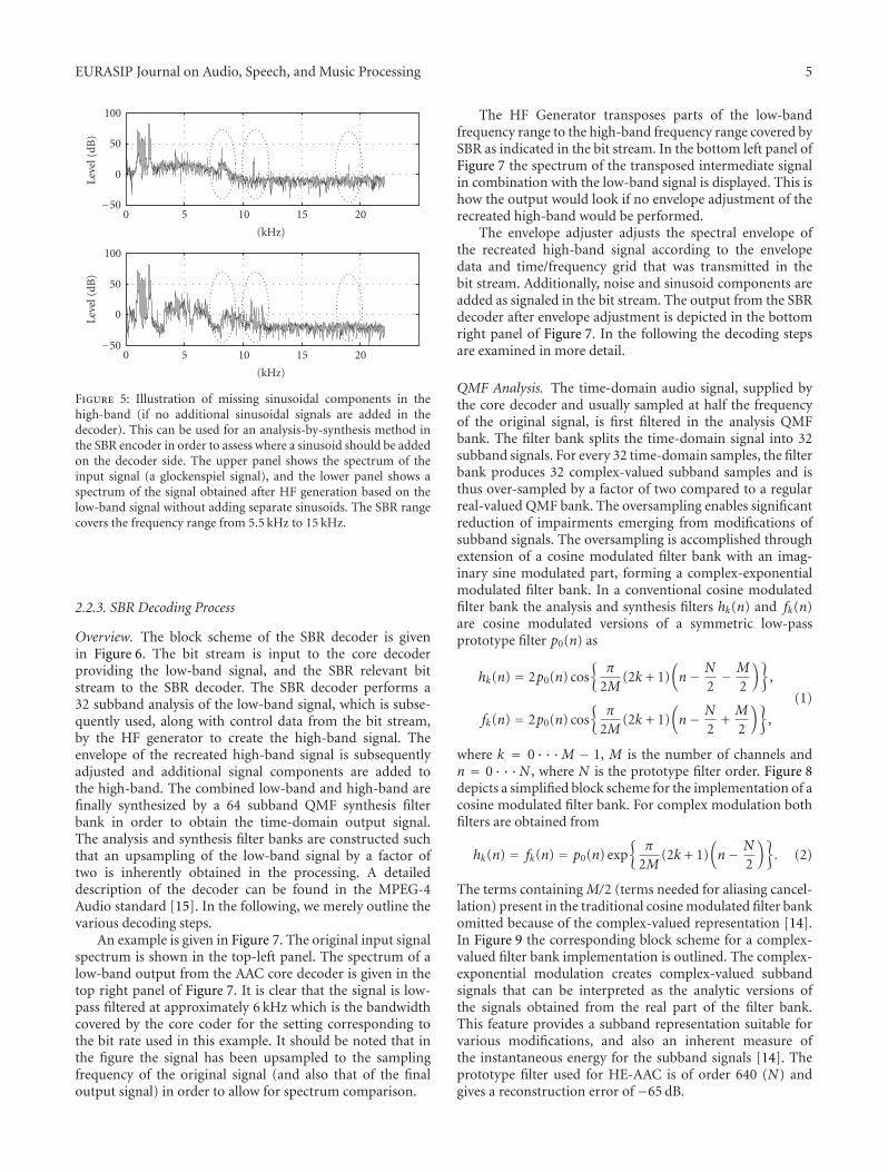
Missing Harmonics Detection. Similarly to the above sit-uation, the encoder also needs to assess whether strongtonal components in the original high-band signal will bemissing after the high-frequency reconstruction. In Figure 5an example is given where three strong tonal componentsare not reconstructed by the high-frequency regenerationbased on the low-band signal. Again an analysis-by-synthesisapproach can be beneficial. For this example a glockenspielsignal is used. In the upper panel of Figure 5 the spectrumfor the input signal is given, where three strong tonalcomponents in the high-band are indicated by circles. In thelower panel of Figure 5 the spectrum of the HF-generatedsignal is given similarly to the example in Figure 4. Clearlythe three strong tonal components will not be properlyregenerated by the HF generator, and therefore need to bereplaced by sinusoids generated separately in the decoder.Information on the (frequency) location of these strong tonalcomponents is transmitted to the decoder, and the missingcomponents are inserted in the high-band signal.

Quantization and Encoding. The SBR envelope data, tonalcomponent data, and noise-floor data are quantized anddifferentially coded in either the time or frequency directionin order to minimize the bit rate. All data is entropy codedusing Huffman tables. Details about SBR data coding aregiven in the next section.

2.2.2. SBR Bit Stream

Overview. To ensure consistent coding of transients regard-less of localization within codec frames, the SBR frames havevariable time boundaries, that is, the exact duration in timecovered by one SBR frame may vary from frame to frame.The bit stream is designed for maximum flexibility suchthat it scales well from the lowest bit rate applications up tomedium and high bit rate use cases, and is easy to adapt for

0.50.40.30.20.10

(s)

0

5

10

15

20

(kH

z)

Figure 3: T/F grid selection example. The white dashed linesillustrate the borders of the time-frequency tiles superimposed onthe spectrogram of the input signal. The leading edge and decayof the transient is encoded with short low frequency resolutionenvelopes, and the quasistationary passages in between transientsare represented by longer high-frequency resolution envelopes.

20151050

(kHz)

−50

0

50

100

Leve

l(dB

)

20151050

(kHz)

−50

0

50

100

Leve

l(dB

)

Figure 4: Illustration of the mismatch in noise level of thereconstructed high-band if no additional noise information istransmitted to the decoder. This can be used for an analysis-by-synthesis method in the SBR encoder in order to assess the amountof noise that should be added on the decoder side. The upperpanel shows the spectrum of the (synthetically generated) inputsignal, and the lower panel shows a spectrum of the signal obtainedafter HF generation based on the low-band signal without noisecorrection. The SBR range covers the frequency range from 5.5 kHzto 15 kHz.

different core codec frame lengths. Furthermore, it is pos-sible to trade bit-error robustness against increased codingefficiency by selecting the degree of interframe dependencies,and the signaling scheme offers error detection capabilities inaddition to a Cyclic Redundancy Check (CRC).


20151050

(kHz)

−50

0

50

100

Leve

l(dB

)

20151050

(kHz)

−50

0

50

100

Leve

l(dB

)

Figure 5: Illustration of missing sinusoidal components in thehigh-band (if no additional sinusoidal signals are added in thedecoder). This can be used for an analysis-by-synthesis method inthe SBR encoder in order to assess where a sinusoid should be addedon the decoder side. The upper panel shows the spectrum of theinput signal (a glockenspiel signal), and the lower panel shows aspectrum of the signal obtained after HF generation based on thelow-band signal without adding separate sinusoids. The SBR rangecovers the frequency range from 5.5 kHz to 15 kHz.

2.2.3. SBR Decoding Process

Overview. The block scheme of the SBR decoder is givenin Figure 6. The bit stream is input to the core decoderproviding the low-band signal, and the SBR relevant bitstream to the SBR decoder. The SBR decoder performs a32 subband analysis of the low-band signal, which is subse-quently used, along with control data from the bit stream,by the HF generator to create the high-band signal. Theenvelope of the recreated high-band signal is subsequentlyadjusted and additional signal components are added tothe high-band. The combined low-band and high-band arefinally synthesized by a 64 subband QMF synthesis filterbank in order to obtain the time-domain output signal.The analysis and synthesis filter banks are constructed suchthat an upsampling of the low-band signal by a factor oftwo is inherently obtained in the processing. A detaileddescription of the decoder can be found in the MPEG-4Audio standard [15]. In the following, we merely outline thevarious decoding steps.

An example is given in Figure 7. The original input signalspectrum is shown in the top-left panel. The spectrum of alow-band output from the AAC core decoder is given in thetop right panel of Figure 7. It is clear that the signal is low-pass filtered at approximately 6 kHz which is the bandwidthcovered by the core coder for the setting corresponding tothe bit rate used in this example. It should be noted that inthe figure the signal has been upsampled to the samplingfrequency of the original signal (and also that of the finaloutput signal) in order to allow for spectrum comparison.

The HF Generator transposes parts of the low-bandfrequency range to the high-band frequency range covered bySBR as indicated in the bit stream. In the bottom left panel ofFigure 7 the spectrum of the transposed intermediate signalin combination with the low-band signal is displayed. This ishow the output would look if no envelope adjustment of therecreated high-band would be performed.

The envelope adjuster adjusts the spectral envelope ofthe recreated high-band signal according to the envelopedata and time/frequency grid that was transmitted in thebit stream. Additionally, noise and sinusoid components areadded as signaled in the bit stream. The output from the SBRdecoder after envelope adjustment is depicted in the bottomright panel of Figure 7. In the following the decoding stepsare examined in more detail.

QMF Analysis. The time-domain audio signal, supplied bythe core decoder and usually sampled at half the frequencyof the original signal, is first filtered in the analysis QMFbank. The filter bank splits the time-domain signal into 32subband signals. For every 32 time-domain samples, the filterbank produces 32 complex-valued subband samples and isthus over-sampled by a factor of two compared to a regularreal-valued QMF bank. The oversampling enables significantreduction of impairments emerging from modifications ofsubband signals. The oversampling is accomplished throughextension of a cosine modulated filter bank with an imag-inary sine modulated part, forming a complex-exponentialmodulated filter bank. In a conventional cosine modulatedfilter bank the analysis and synthesis filters hk(n) and fk(n)are cosine modulated versions of a symmetric low-passprototype filter p0(n) as

hk(n) = 2p0(n) cos{

π

2M(2k + 1)

(n− N

2− M

2

)},

fk(n) = 2p0(n) cos{

π

2M(2k + 1)

(n− N

2+M

2

)},

(1)

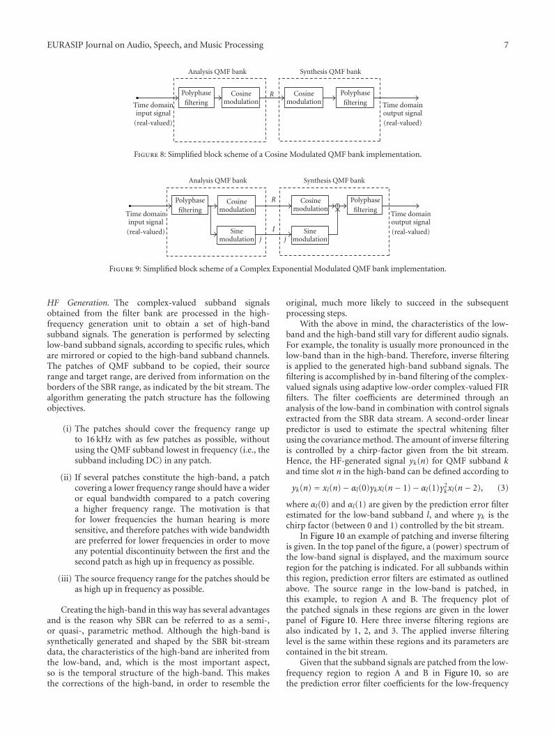
where k = 0 · · ·M − 1, M is the number of channels andn = 0 · · ·N , where N is the prototype filter order. Figure 8depicts a simplified block scheme for the implementation of acosine modulated filter bank. For complex modulation bothfilters are obtained from

hk(n) = fk(n) = p0(n) exp{

π

2M(2k + 1)

(n− N

2

)}. (2)

The terms containing M/2 (terms needed for aliasing cancel-lation) present in the traditional cosine modulated filter bankomitted because of the complex-valued representation [14].In Figure 9 the corresponding block scheme for a complex-valued filter bank implementation is outlined. The complex-exponential modulation creates complex-valued subbandsignals that can be interpreted as the analytic versions ofthe signals obtained from the real part of the filter bank.This feature provides a subband representation suitable forvarious modifications, and also an inherent measure ofthe instantaneous energy for the subband signals [14]. Theprototype filter used for HE-AAC is of order 640 (N) andgives a reconstruction error of −65 dB.


SBR decoder

BitstreamCore

decoder

Audio

signal

fs

SBRdata

QMFanalysis

(32 bands)

HFgenerator

Envelopeadjuster

AdditionalHF

components

QMFsynthesis

(64 bands)

Audio

output2 fs

Uncompressed audio signalData path

Figure 6: Block scheme of the SBR decoder. The received bit stream is input to the core decoder decoding the low-band audio signal,and providing the SBR decoder with the SBR relevant bit stream data. The SBR decoder performs a QMF analysis of the low-band signalwhich is subsequently used for the HF Generation providing a high-band signal. The high-band is envelope adjusted and additional signalcomponents are added. Finally, the output signal is obtained by a QMF synthesis filter bank.

20151050

Frequency (kHz)

−50

0

50

Leve

l(dB

)

Original

20151050

Frequency (kHz)

−50

0

50

Leve

l(dB

)

AAC output

20151050

Frequency (kHz)

−50

0

50

Leve

l(dB

)

HF generation

20151050

Frequency (kHz)

−50

0

50

Leve

l(dB

)

aacPlus output

Figure 7: Spectrum of the signal at different points of processing in the SBR decoder. Top left is the (power) spectrum of the original signal,top right is the spectrum of the low-band signal resulting from the AAC decoder, bottom left is the spectrum of the combined low-band andhigh-band prior to envelope adjustment, bottom right is the spectrum of the output signal.


Analysis QMF bank

Time domaininput signal

(real-valued)

Polyphasefiltering

Cosinemodulation

R

Synthesis QMF bank

Cosinemodulation

Polyphasefiltering Time domain

output signal(real-valued)

Figure 8: Simplified block scheme of a Cosine Modulated QMF bank implementation.

Analysis QMF bank

Time domaininput signal

(real-valued)

Polyphasefiltering

Cosinemodulation

Sinemodulation

R

I

j j

Synthesis QMF bank

Cosinemodulation +

Polyphasefiltering

Sinemodulation

Time domainoutput signal(real-valued)

Figure 9: Simplified block scheme of a Complex Exponential Modulated QMF bank implementation.

HF Generation. The complex-valued subband signalsobtained from the filter bank are processed in the high-frequency generation unit to obtain a set of high-bandsubband signals. The generation is performed by selectinglow-band subband signals, according to specific rules, whichare mirrored or copied to the high-band subband channels.The patches of QMF subband to be copied, their sourcerange and target range, are derived from information on theborders of the SBR range, as indicated by the bit stream. Thealgorithm generating the patch structure has the followingobjectives.

(i) The patches should cover the frequency range upto 16 kHz with as few patches as possible, withoutusing the QMF subband lowest in frequency (i.e., thesubband including DC) in any patch.

(ii) If several patches constitute the high-band, a patchcovering a lower frequency range should have a wideror equal bandwidth compared to a patch coveringa higher frequency range. The motivation is thatfor lower frequencies the human hearing is moresensitive, and therefore patches with wide bandwidthare preferred for lower frequencies in order to moveany potential discontinuity between the first and thesecond patch as high up in frequency as possible.

(iii) The source frequency range for the patches should beas high up in frequency as possible.

Creating the high-band in this way has several advantagesand is the reason why SBR can be referred to as a semi-,or quasi-, parametric method. Although the high-band issynthetically generated and shaped by the SBR bit-streamdata, the characteristics of the high-band are inherited fromthe low-band, and, which is the most important aspect,so is the temporal structure of the high-band. This makesthe corrections of the high-band, in order to resemble the

original, much more likely to succeed in the subsequentprocessing steps.

With the above in mind, the characteristics of the low-band and the high-band still vary for different audio signals.For example, the tonality is usually more pronounced in thelow-band than in the high-band. Therefore, inverse filteringis applied to the generated high-band subband signals. Thefiltering is accomplished by in-band filtering of the complex-valued signals using adaptive low-order complex-valued FIRfilters. The filter coefficients are determined through ananalysis of the low-band in combination with control signalsextracted from the SBR data stream. A second-order linearpredictor is used to estimate the spectral whitening filterusing the covariance method. The amount of inverse filteringis controlled by a chirp-factor given from the bit stream.Hence, the HF-generated signal yk(n) for QMF subband kand time slot n in the high-band can be defined according to

yk(n) = xl(n)− αl(0)γkxl(n− 1)− αl(1)γ2kxl(n− 2), (3)

where αl(0) and αl(1) are given by the prediction error filterestimated for the low-band subband l, and where γk is thechirp factor (between 0 and 1) controlled by the bit stream.

In Figure 10 an example of patching and inverse filteringis given. In the top panel of the figure, a (power) spectrum ofthe low-band signal is displayed, and the maximum sourceregion for the patching is indicated. For all subbands withinthis region, prediction error filters are estimated as outlinedabove. The source range in the low-band is patched, inthis example, to region A and B. The frequency plot ofthe patched signals in these regions are given in the lowerpanel of Figure 10. Here three inverse filtering regions arealso indicated by 1, 2, and 3. The applied inverse filteringlevel is the same within these regions and its parameters arecontained in the bit stream.

Given that the subband signals are patched from the low-frequency region to region A and B in Figure 10, so arethe prediction error filter coefficients for the low-frequency


20151050

Frequency (kHz)

−50

0

50

Leve

l(dB

)

AAC lowband signal

Frequency range used forHF patch and estimation

of filter coefficients

A B

20151050

Frequency (kHz)

−50

0

50

Leve

l(dB

)

HF Generated highband signal

1 2 3

Frequency range of

first HF patch

Frequency range of

second HF patch

Frequency ranges of

inverse filtering bands

Figure 10: Example of high-frequency generation and inversefiltering. The figure shows the frequency spectra of the low-band signal and the subsequent high-band signals. The signalis an excerpt of a classical music piece coded at 24 kbps mono.The frequency range for SBR, as given in the bit stream for theconfiguration used, is 5.5 kHz to 15 kHz. This range is covered bytwo consecutive patches, A and B, where A has a larger frequencyrange. Finally, three inverse filtering regions are given by the bitstream, where the frequency border of the second and third regioncoincide with the patch border.

region. Thus, the suitable prediction error filter coefficientsare available for all subbands within region A and B. Hence,for all the QMF subbands within the region 1 in Figure 10an inverse filtering is done within each subband, giventhe corresponding prediction error filter estimated on thecorresponding low-band subband samples and the chirpfactor signaled in the bit stream for the specific region.

It should be noted that all the processing done in the HFGeneration module is done frame-based on a time segmentindicated by the outer borders of the SBR frame.

The generated high-band signals are subsequently fed tothe envelope adjusting unit.

Envelope Adjustment. The most important, and also thelargest part of the SBR data stream, is the spectrotemporalenvelope representation of the high-band. This enveloperepresentation is used to adjust the energy of the generatedhigh-band subband signals. The envelope adjusting unit firstperforms an energy estimate of the high-band signals. Anaccurate estimate is possible because of the complex-valuedsubband signal representation. The resulting energy samplesare subsequently averaged within segments according tocontrol signals from the data stream. This averaging producesthe estimated envelope samples. Based on the estimatedenvelope and the envelope representation extracted from the

data stream, the energy of the high-band subband samples inthe respective segments are adjusted.

As previously outlined sinusoids present in the originalhigh-band signal that have no corresponding sinusoid inthe generated high-band are synthesized in the decoder, andrandom white noise is added to the high-band signal tocompensate for diverging tonal-to-noise ratios of the high-band and low-band.

A noise floor level Q is used to derive the level of noiseto be added to the recreated high-band signal, it is definedas the energy ratio between the HF-generated (by means ofpatching in the HF generator) signal energy and the noisesignal energy of the final output signal.

Given the calculated gain values, a limiting procedureis applied. This is designed to avoid the need to excessivelyhigh-gain values due to large differences in the transposedsignal energy and the reference energy given by the originalinput signal. The limiter is operative to limit high narrow-band gain values while ensuring that the correct wide-bandenergy is maintained.

QMF Synthesis. The generated high-band signals and thedelay-compensated (resulting from the HF generation pro-cess) low-band signals are finally supplied to the 64-channelsynthesis filter bank, which usually operates at the samplingfrequency of the original signal. The synthesis filter bankis just like the analysis filter bank complex-valued, howeverthe imaginary part of the output signal is discarded. Thus,the filter bank generates a real-valued full bandwidth outputsignal having twice the sampling frequency of the core codersignal.

2.2.4. Other Aspects

Low Power SBR. The SBR tool as outlined in the previoussections is defined in two versions: a High Quality Versionand a Low-Power version. The main difference is that theLow-Power version utilizes real-valued QMF filter banks,while the High Quality version utilizes complex-valued filterbanks. In order to make the SBR Tool work in the real-valueddomain, additional tools are included that strive to minimizethe introduction of aliasing in the SBR processing. Themain feature is an aliasing detection algorithm that identifiesadjacent QMF subbands with strong tonal components inthe overlapping range. The detection is done by studying thereflection coefficient of a first-order in-band linear predictor.By observing the signs of the reflection coefficients foradjacent subbands, the subbands prone to introduce aliasingcan be identified. For the identified subbands restrictions areput on how much the gain adjustment is allowed to varybetween the two subbands.

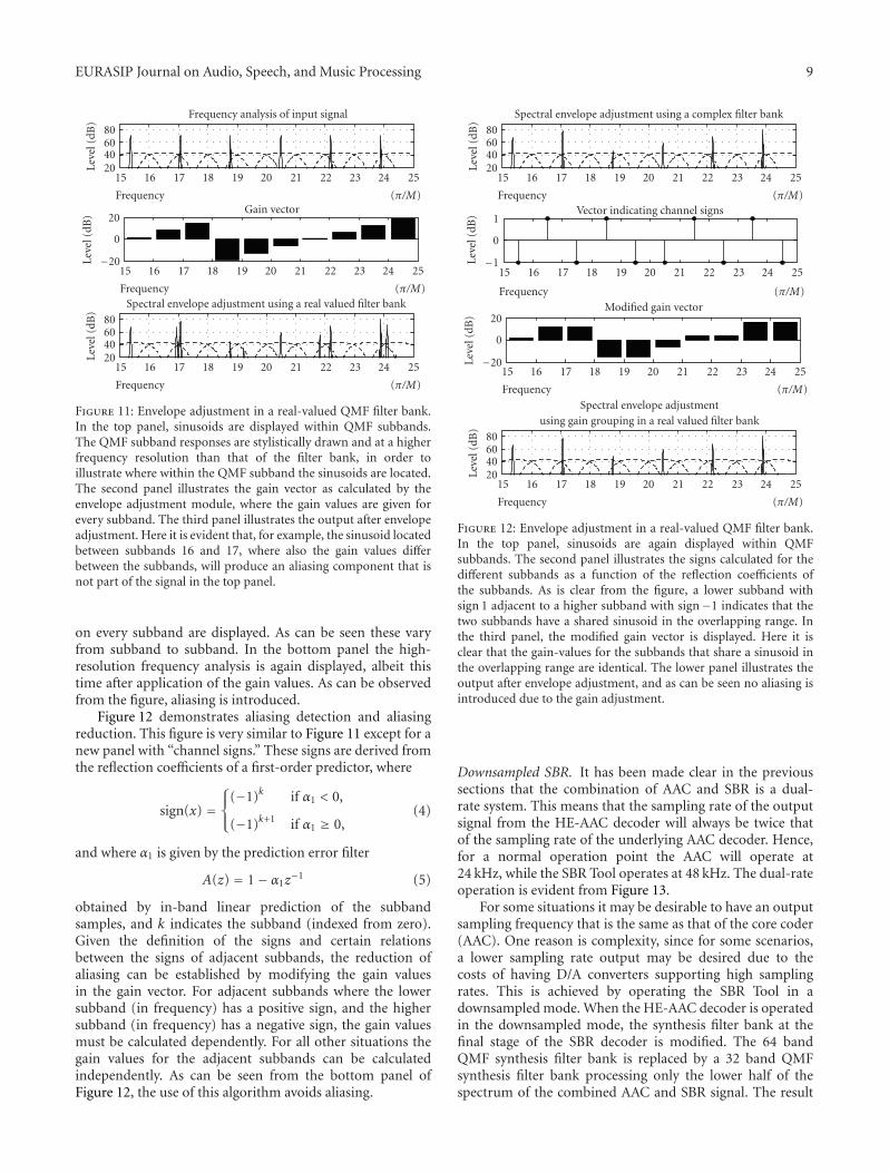
The following text and figures provide an example of low-power SBR. Envelope adjustment in a real-valued QMF filterbank is displayed in Figure 11.

The upper panel of the Figure 11 illustrates a high-resolution frequency analysis of the input signal superim-posed on a stylized visualization of the QMF frequencyresponse. In the middle panel the gain values to be applied


2524232221201918171615

Frequency (π/M)

20406080

Leve

l(dB

)

Frequency analysis of input signal

2524232221201918171615

Frequency (π/M)

−20

0

20

Leve

l(dB

)

Gain vector

2524232221201918171615

Frequency (π/M)

20406080

Leve

l(dB

)

Spectral envelope adjustment using a real valued filter bank

Figure 11: Envelope adjustment in a real-valued QMF filter bank.In the top panel, sinusoids are displayed within QMF subbands.The QMF subband responses are stylistically drawn and at a higherfrequency resolution than that of the filter bank, in order toillustrate where within the QMF subband the sinusoids are located.The second panel illustrates the gain vector as calculated by theenvelope adjustment module, where the gain values are given forevery subband. The third panel illustrates the output after envelopeadjustment. Here it is evident that, for example, the sinusoid locatedbetween subbands 16 and 17, where also the gain values differbetween the subbands, will produce an aliasing component that isnot part of the signal in the top panel.

on every subband are displayed. As can be seen these varyfrom subband to subband. In the bottom panel the high-resolution frequency analysis is again displayed, albeit thistime after application of the gain values. As can be observedfrom the figure, aliasing is introduced.

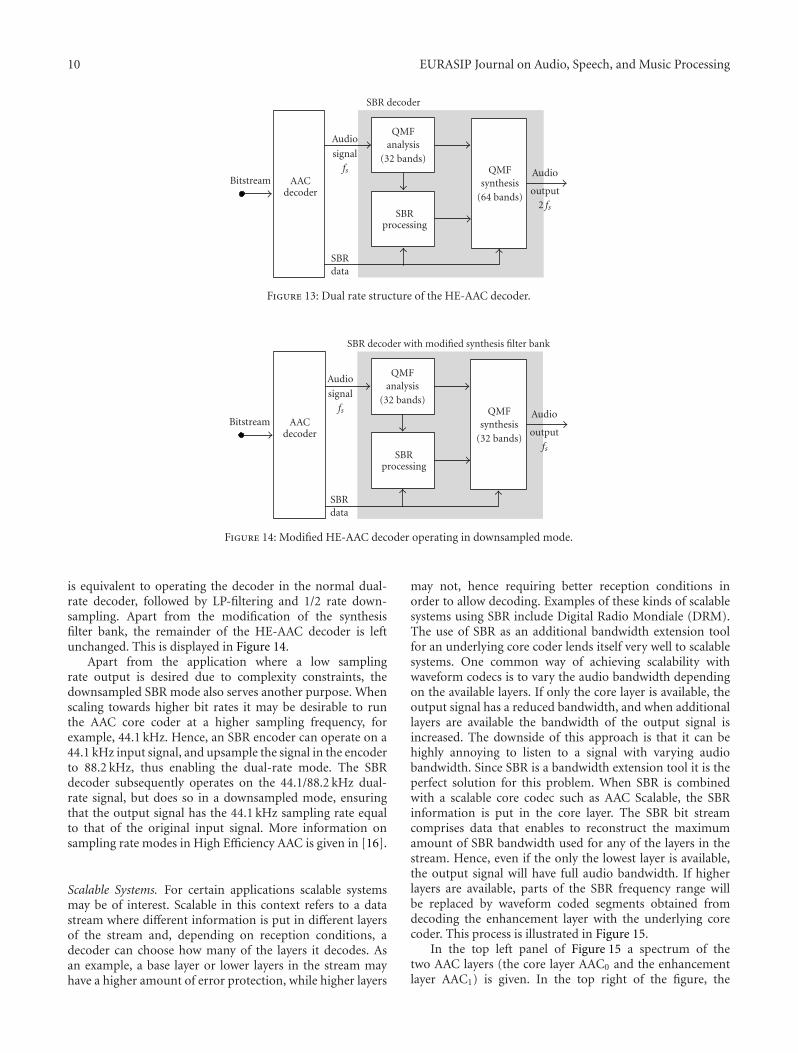
Figure 12 demonstrates aliasing detection and aliasingreduction. This figure is very similar to Figure 11 except for anew panel with “channel signs.” These signs are derived fromthe reflection coefficients of a first-order predictor, where

sign(x) =⎧⎨⎩

(−1)k if α1 < 0,

(−1)k+1 if α1 ≥ 0,(4)

and where α1 is given by the prediction error filter

A(z) = 1− α1z−1 (5)

obtained by in-band linear prediction of the subbandsamples, and k indicates the subband (indexed from zero).Given the definition of the signs and certain relationsbetween the signs of adjacent subbands, the reduction ofaliasing can be established by modifying the gain valuesin the gain vector. For adjacent subbands where the lowersubband (in frequency) has a positive sign, and the highersubband (in frequency) has a negative sign, the gain valuesmust be calculated dependently. For all other situations thegain values for the adjacent subbands can be calculatedindependently. As can be seen from the bottom panel ofFigure 12, the use of this algorithm avoids aliasing.

2524232221201918171615

Frequency (π/M)

20406080

Leve

l(dB

)

Spectral envelope adjustment using a complex filter bank

2524232221201918171615

Frequency (π/M)

−1

0

1

Leve

l(dB

) Vector indicating channel signs

2524232221201918171615

Frequency (π/M)

−20

0

20

Leve

l(dB

)

Modified gain vector

2524232221201918171615

Frequency (π/M)

20406080

Leve

l(dB

)

Spectral envelope adjustmentusing gain grouping in a real valued filter bank

Figure 12: Envelope adjustment in a real-valued QMF filter bank.In the top panel, sinusoids are again displayed within QMFsubbands. The second panel illustrates the signs calculated for thedifferent subbands as a function of the reflection coefficients ofthe subbands. As is clear from the figure, a lower subband withsign 1 adjacent to a higher subband with sign−1 indicates that thetwo subbands have a shared sinusoid in the overlapping range. Inthe third panel, the modified gain vector is displayed. Here it isclear that the gain-values for the subbands that share a sinusoid inthe overlapping range are identical. The lower panel illustrates theoutput after envelope adjustment, and as can be seen no aliasing isintroduced due to the gain adjustment.

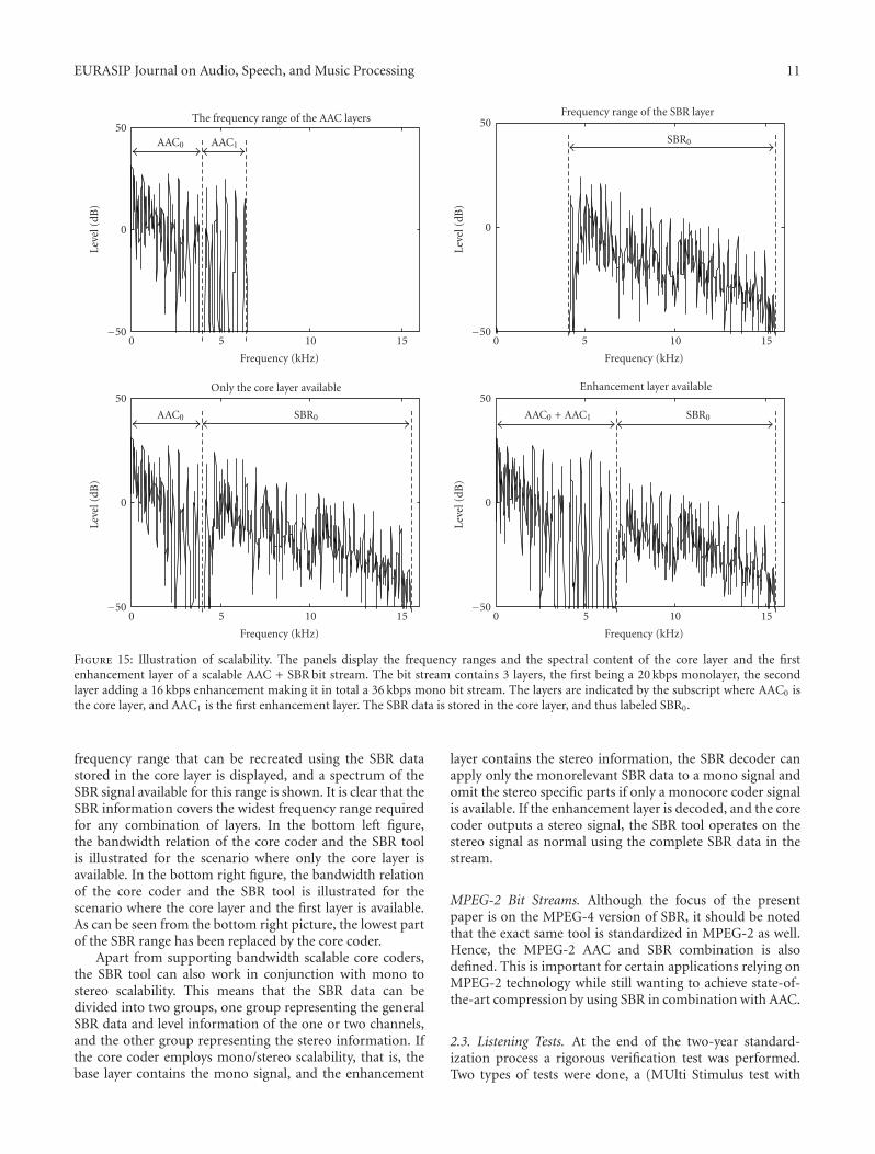
Downsampled SBR. It has been made clear in the previoussections that the combination of AAC and SBR is a dual-rate system. This means that the sampling rate of the outputsignal from the HE-AAC decoder will always be twice thatof the sampling rate of the underlying AAC decoder. Hence,for a normal operation point the AAC will operate at24 kHz, while the SBR Tool operates at 48 kHz. The dual-rateoperation is evident from Figure 13.

For some situations it may be desirable to have an outputsampling frequency that is the same as that of the core coder(AAC). One reason is complexity, since for some scenarios,a lower sampling rate output may be desired due to thecosts of having D/A converters supporting high samplingrates. This is achieved by operating the SBR Tool in adownsampled mode. When the HE-AAC decoder is operatedin the downsampled mode, the synthesis filter bank at thefinal stage of the SBR decoder is modified. The 64 bandQMF synthesis filter bank is replaced by a 32 band QMFsynthesis filter bank processing only the lower half of thespectrum of the combined AAC and SBR signal. The result


SBR decoder

Bitstream AACdecoder

Audio

signal

fs

SBRdata

QMFanalysis

(32 bands)

SBRprocessing

QMFsynthesis

(64 bands)

Audio

output2 fs

Figure 13: Dual rate structure of the HE-AAC decoder.

SBR decoder with modified synthesis filter bank

Bitstream AACdecoder

Audio

signal

fs

SBRdata

QMFanalysis

(32 bands)

SBRprocessing

QMFsynthesis

(32 bands)

Audio

outputfs

Figure 14: Modified HE-AAC decoder operating in downsampled mode.

is equivalent to operating the decoder in the normal dual-rate decoder, followed by LP-filtering and 1/2 rate down-sampling. Apart from the modification of the synthesisfilter bank, the remainder of the HE-AAC decoder is leftunchanged. This is displayed in Figure 14.

Apart from the application where a low samplingrate output is desired due to complexity constraints, thedownsampled SBR mode also serves another purpose. Whenscaling towards higher bit rates it may be desirable to runthe AAC core coder at a higher sampling frequency, forexample, 44.1 kHz. Hence, an SBR encoder can operate on a44.1 kHz input signal, and upsample the signal in the encoderto 88.2 kHz, thus enabling the dual-rate mode. The SBRdecoder subsequently operates on the 44.1/88.2 kHz dual-rate signal, but does so in a downsampled mode, ensuringthat the output signal has the 44.1 kHz sampling rate equalto that of the original input signal. More information onsampling rate modes in High Efficiency AAC is given in [16].

Scalable Systems. For certain applications scalable systemsmay be of interest. Scalable in this context refers to a datastream where different information is put in different layersof the stream and, depending on reception conditions, adecoder can choose how many of the layers it decodes. Asan example, a base layer or lower layers in the stream mayhave a higher amount of error protection, while higher layers

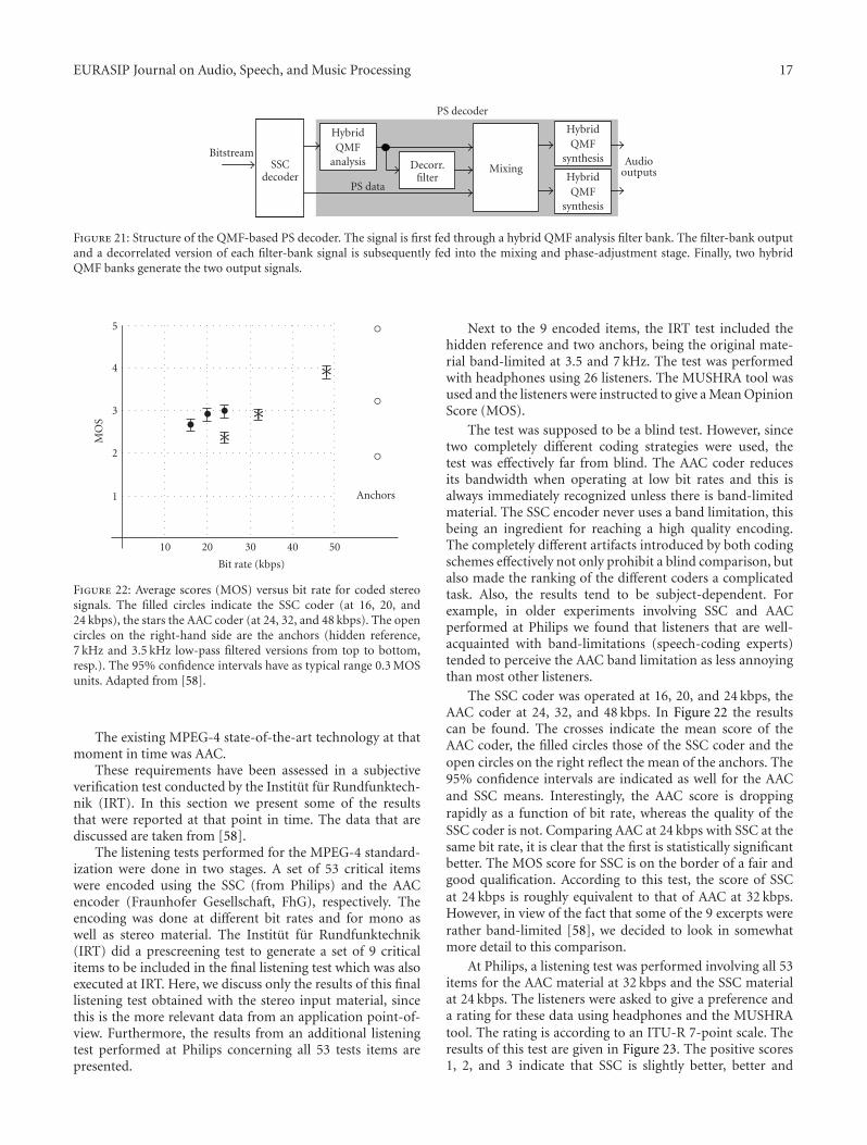
may not, hence requiring better reception conditions inorder to allow decoding. Examples of these kinds of scalablesystems using SBR include Digital Radio Mondiale (DRM).The use of SBR as an additional bandwidth extension toolfor an underlying core coder lends itself very well to scalablesystems. One common way of achieving scalability withwaveform codecs is to vary the audio bandwidth dependingon the available layers. If only the core layer is available, theoutput signal has a reduced bandwidth, and when additionallayers are available the bandwidth of the output signal isincreased. The downside of this approach is that it can behighly annoying to listen to a signal with varying audiobandwidth. Since SBR is a bandwidth extension tool it is theperfect solution for this problem. When SBR is combinedwith a scalable core codec such as AAC Scalable, the SBRinformation is put in the core layer. The SBR bit streamcomprises data that enables to reconstruct the maximumamount of SBR bandwidth used for any of the layers in thestream. Hence, even if the only the lowest layer is available,the output signal will have full audio bandwidth. If higherlayers are available, parts of the SBR frequency range willbe replaced by waveform coded segments obtained fromdecoding the enhancement layer with the underlying corecoder. This process is illustrated in Figure 15.

In the top left panel of Figure 15 a spectrum of thetwo AAC layers (the core layer AAC0 and the enhancementlayer AAC1) is given. In the top right of the figure, the


151050

Frequency (kHz)

−50

0

50

Leve

l(dB

)

The frequency range of the AAC layers

AAC0 AAC1

151050

Frequency (kHz)

−50

0

50

Leve

l(dB

)

Frequency range of the SBR layer

SBR0

151050

Frequency (kHz)

−50

0

50

Leve

l(dB

)

Only the core layer available

AAC0 SBR0

151050

Frequency (kHz)

−50

0

50

Leve

l(dB

)

Enhancement layer available

AAC0 + AAC1 SBR0

Figure 15: Illustration of scalability. The panels display the frequency ranges and the spectral content of the core layer and the firstenhancement layer of a scalable AAC + SBR bit stream. The bit stream contains 3 layers, the first being a 20 kbps monolayer, the secondlayer adding a 16 kbps enhancement making it in total a 36 kbps mono bit stream. The layers are indicated by the subscript where AAC0 isthe core layer, and AAC1 is the first enhancement layer. The SBR data is stored in the core layer, and thus labeled SBR0.

frequency range that can be recreated using the SBR datastored in the core layer is displayed, and a spectrum of theSBR signal available for this range is shown. It is clear that theSBR information covers the widest frequency range requiredfor any combination of layers. In the bottom left figure,the bandwidth relation of the core coder and the SBR toolis illustrated for the scenario where only the core layer isavailable. In the bottom right figure, the bandwidth relationof the core coder and the SBR tool is illustrated for thescenario where the core layer and the first layer is available.As can be seen from the bottom right picture, the lowest partof the SBR range has been replaced by the core coder.

Apart from supporting bandwidth scalable core coders,the SBR tool can also work in conjunction with mono tostereo scalability. This means that the SBR data can bedivided into two groups, one group representing the generalSBR data and level information of the one or two channels,and the other group representing the stereo information. Ifthe core coder employs mono/stereo scalability, that is, thebase layer contains the mono signal, and the enhancement

layer contains the stereo information, the SBR decoder canapply only the monorelevant SBR data to a mono signal andomit the stereo specific parts if only a monocore coder signalis available. If the enhancement layer is decoded, and the corecoder outputs a stereo signal, the SBR tool operates on thestereo signal as normal using the complete SBR data in thestream.

MPEG-2 Bit Streams. Although the focus of the presentpaper is on the MPEG-4 version of SBR, it should be notedthat the exact same tool is standardized in MPEG-2 as well.Hence, the MPEG-2 AAC and SBR combination is alsodefined. This is important for certain applications relying onMPEG-2 technology while still wanting to achieve state-of-the-art compression by using SBR in combination with AAC.

2.3. Listening Tests. At the end of the two-year standard-ization process a rigorous verification test was performed.Two types of tests were done, a (MUlti Stimulus test with


Table 1: Codecs under test.

Coding scheme LabelBit rate Sampling rate Typical audio bandwidth

(mono/stereo) (kHz) (kHz)

MPEG-4 AAC profile AAC 48/60 kbps 48/60 kbps 32 10/13.5

MPEG-4 HE-AAC HE-AAC 32/48 kbps 32/48 kbps 24/48 15.5

Anchors and reference Hidden reference 16-bit PCM stereo 48 24

Anchors and reference Anchor 3.5 kHz 16-bit PCM stereo 48 3.5

Anchors and reference Anchor 7 kHz 16-bit PCM stereo 48 7.0

HE-AAC24 kbps

AAC30 kbps

AAC24 kbps

Anchor3.5 kHz

Anchor7 kHz

Hiddenreference

0

20

40

60

80

10099.8

57.3

25.4

Mean value

45.6 52.5

95% conf.75.2

Figure 16: Listening test results for mono MUSHRA tests. Thescores are the average scores over all items and test-sites (adaptedfrom [19]).

Hidden Reference and Anchor) MUSHRA test [17] and a(Comparative Mean Opinion Score) CMOS test [18]. TheMUSHRA test compared the performance of MPEG-4 HE-AAC with that of MPEG-4 AAC when coding mono andstereo signals at bit rates in the range 24 kbps per channel,while the CMOS test was used to show the difference betweenHigh Quality SBR and Low Power SBR. Two test sets wereselected, one for mono testing, and one for stereo testing.The items were selected from 50 potential candidates by aselection panel identifying ten items considered critical forall of the systems under test.

The codecs under test for the verification tests areoutlined in Table 1. The listening tests were performed atFrance Telecom, T-Systems Nova, Panasonic, NEC, andCoding Technologies.

The listening test results are presented in Figures 16 and17. From the listening tests it is clear that the SBR enhancedAAC technology (High Efficiency AAC Profile) performsbetter than the MPEG-4 AAC Profile when the latter isoperating at a 25% higher bit rate (i.e., 30 versus 24 kbps formono, and 60 versus 48 kbps for stereo).

The SBR technology in combination with AAC asstandardized in MPEG under the name High Efficiency AAC(also known as aacPlus) offers a substantial improvement incompression efficiency compared to previous state-of-the-art codecs. It is the first audio codec to offer full bandwidthaudio at good quality at low bit-rate. This makes it the idealcodec (and enabler) for low bit-rate applications such asDigital Radio Mondiale and streaming to mobile phones.

3. MPEG-4 SSC

3.1. Parametric Mono Coding. Current standardized andproprietary coding schemes are primarily build basedon waveform coding techniques. These coding algorithms

HE-AAC48 kbps

HE-AAC32 kbps

AAC60 kbps

AAC48 kbps

Anchor3.5 kHz

Anchor7 kHz

Hiddenreference

0

20

40

60

80

10097

32.3

13.5

Mean value

37.5

66.4

95% conf.

56.773.2

Figure 17: Listening test results for stereo MUSHRA tests Thescores are the average scores over all items and test-sites (adaptedfrom [19]).

translate the incoming signal to the frequency domain byuse of a subband or transform technique. Furthermore, apsychoacoustic model analyzes the incoming signal as welland determines the number of bits for quantization of eachof the subband or transform signals. For an overview, see[20].

The subband or transform audio coding schemes primar-ily exploit the destination (human ear) model; the psychoa-coustic model tells us where signal distortions (quantization)are allowed such that these are inaudible or least annoying.In speech coding, on the other hand, source models areprimarily used. The incoming signal is matched to thecharacteristics of a source model (the vocal tract model), andthe parameters of this source model are transmitted. In thedecoder, the source model and its parameters are used toreconstruct the signal. For an overview on speech coding,please refer to [21].

The speech coding approach guarantees that the repro-duced signal is in accordance with the model. This impliesthat if the model is an accurate description, the generatedsignal will sound like stemming from a vocal tract and willtherefore sound natural though not necessarily identical tothe incoming signal.

For audio, it is not possible to directly follow an approachlike in speech coding. There are many sources in audio andthese have quite different characteristics. The consequencesof using a too restrictive source models can be devastatingto the sound quality. This is already demonstrated by speechcoders operating at low bit-rates; input signals other thanspeech typically result in a poor quality of the decodedoutput signals.

Nevertheless, a model is used in parametric coding.This is called a signal model to distinguish it from sourcemodels as are used in speech coding. The origin of thesignal model is more based on destination properties


Bitstream BSP

TrS

SiS

NoS

x

Figure 18: Decoder scheme producing the decoded signal x fromthe bit stream. The decoding consists of a bit stream parser (BSP),a transient synthesizer (Trs), a sinusoidal synthesizer (SiS), and anoise synthesizer (NoS).

(i.e., the human hearing system) in the sense that it triesto describe perceptually-relevant acoustic events. Conse-quently, parametric coding is also related to musical synthe-sis. However, the distinction between source and destinationmodels is arguable; for example, many musical instrumentscreate tonal components and biological evolution presum-ably leads to a tight connection between destination andsource characteristics.

The promises that the parametric approach holds aretherefore as follows. First of all, the signal model shouldalways lead to an impression of an agreeable sound even atlow bit rates. Thus a graceful degradation of sound qualitywith bit rate should be feasible. This is a property which isdifficult to attain in conventional audio coding techniques.Secondly, since the idea is to model acoustic events, we maybe able to manipulate these events (like in musical synthesis),a feature clearly not feasible in conventional audio coding.

At various universities, prototype parametric audiocoders have been developed [22–29]. Prior to the parametriccoder described in this paper, there was only one standard-ized parametric audio coder: HILN [30] in MPEG-4 AudioVersion 2 [31].

In the Sinusoidal Coder (SSC) that is described hereand which is standardized in MPEG-4, three objects can bediscerned. The first one comprises tonal components. Theseare modeled by sinusoids. This idea seems to be originatedfrom speech coding [32–34]. The second one is a noiseobject. Also this object is present in speech coders, only theresegments are typically denoted as either voiced or unvoiced,corresponding to noise and periodic excitations. In audio, anearly reference to simultaneous use of sinusoidal and noisecoding is [35].

Both sinusoidal modeling and noise modeling assumethat the signal segment being modeled is stationary. Inview of bit rate and frequency resolution, these segmentsmay not be too short. Consequently, one can find audiosegments that, given the analysis segment length, containclearly instationary events. A famous example forms thecastanets excerpt, which is therefore a critical item for almostany coder. In view of this, it was decided to introduce a thirdobject which is the transients. The coder not only uses aseparate transient object but also adapts the windowing forthe sinusoidal and noise analysis and synthesis on basis ofdetected transients.

3.1.1. SSC Decoder

Overview. The SSC decoder is depicted in Figure 18. Asdescribed in the previous section, the idea is that a monoaudio signal can be described by three basic signal compo-nents: transients, sinusoids, and noise. The information onthese components is contained in the bit stream and thedecoder uses a parser Bit Stream Parser (BSP) to split thisstream. The three basic signal components are decoded usinga transient, sinusoidal, and noise synthesizer (TrS, SiS, andNoS, resp.). Adding these signals gives a decoded mono audiosignal (x).

A detailed description of the decoder can be found in theMPEG-4 document [36]. In the following, we merely outlinethe operations of the different modules.

Transient Synthesis. The bit stream contains transient infor-mation. First of all, transient positions are transmittedtogether with a type parameter. There are two types: a step-like transient and a Meixner transient. In both cases, thetransient position is used to generate adapted overlap-addwindows for the sinusoidal and noise synthesis. Thus thisinformation is shared by the three synthesizers TrS, SiS, andNoS.

In the case of a Meixner window, a Meixner envelopeis created and multiplied by a number of sinusoids thusdefining a transient phenomenon [37–39]. The discrete-timeMeixner envelope is given by

g(n) = (1− ξ2)b/2√

(b)nn!

ξn, (6)

with b > 0, 0 < ξ < 1 and n = 0, 1, . . . . The parametersb and ξ define the rise and decay time of the transientenvelope. In case of a step-like transient, no signal is createdby the transient generator. However, due to the use of theadapted overlap-add windows in the sinusoidal and noisesynthesizers, a transient phenomenon is created in the monosignal x for the step transient as well.

Sinusoidal Synthesis. The sinusoidal data is contained in so-called sinusoidal tracks. From these tracks, information onthe number of sinusoids, their frequencies, amplitudes, andphases is available for each frame. These signals are generatedto produce a waveform per frame. Typically, the frames areoverlap-added using an amplitude-complementary Hanningwindow with 50% overlap. In case of a transient, fade-in orfade-out of these overlap-add windows are shortened andpositioned around the pertinent transient position.

Noise Synthesis. The noise synthesizer consists of a whitenoise generator with unit variance. The bit streams containsdata concerning the temporal envelope per 4 frames. Theenvelope is generated [39] and applied to the noise. Next,this temporally shaped noise is an input to a linear predictionsynthesis filter based on Laguerre filter [40]. The data onthe filter coefficients are contained in the bit stream perframe. The generated noise is overlap added using powercomplimentary windows.


Bitstream

TrD

TrA

TrS

SiA

SiS

NoA

x

r1 −

r2 −

BSF

Figure 19: Encoder scheme producing a bit stream from an audiosignal. It consists of a transient detector (TrD), a transient analyzer(TrA), a sinusoidal analyzer (SiA), a noise analyzer (NoA), and a bitstream formatter (BSF).

3.1.2. SSC Encoder

Overview. The SSC encoder is not standardized by MPEGand as such several designs are possible. We will discuss thestructure of the encoder we developed and different possiblemechanisms within this structure.

The mono encoding scheme (Figure 19) implements theopposite process to the decoder in a cascaded manner. Thecoder analyzes the input signal x and describes it as a sumof three basic components. To this end, it uses a transientdetector (TrD) which detects transients and estimates theirstarting position. This information is fed to the transientanalysis (TrA) which estimates the transient componentparameters and feeds these to a transient synthesizer. In thetransient synthesizer (TrS), the estimated waveform capturedin the transient parameters is generated and subtracted fromthe input signal, thus making a first residual r1.

The first residual is an input to a sinusoidal analyzer(SiA) which also uses the estimated transient positions.This information is exploited in order to prevent measuringover nonstationary data which is done by adaptation ofthe analysis windows. The sinusoidal parameters are fed toa sinusoidal synthesizer (SiS) which generates a waveform.This waveform is subtracted from the first residual signalthus generating a second residual signal r2.

The signal r2 is fed to a noise analyzer (NoA). Thisanalyzer tries to capture the spectral and temporal envelopesof the remaining signal ignoring its specific waveform. Alsoin this analysis module, the transient position estimates areused for window adaptation.

The parameter streams generated by the transient detec-tor and the various analysis stages are fed to a bit stream

formatter (BSF). At this stage, irrelevancy and redundancyof the parameter streams are exploited and the data isquantized. The quantized data is stored in a bit stream.

Though the concept of separation in these three differentobjects is similar to the work presented in [41], there arelarge differences between the approaches. This holds for thedifferent models which are used for the noise and transientcomponents, but also in the sense that [41] subdividesthe input signal in time-frequency tiles where each tile isexclusively modeled by one of the three components.

Transient Analysis. The transient analysis is only performedwhen the transient detector signals the occurrence of asudden change in the input signal. The detector can be buildon basis of detection of changes of energy [42] where thesechanges are defined over the entire frequency range or overdifferent frequency bands. Next to detection of a transient,the detector estimates the start position of the transient.

When the transient detector signals the occurrenceof a transient in a frame, the transient analysis modulebecomes active. On basis of the input signal and the receivedtransient start position, it first determines the character ofthe transient. If the transient phenomenon is shorter than theanalysis frame lengths used in the sinusoidal and noise anal-ysis (typically in the order of tens of milliseconds), a Meixnermodeling stage becomes active. Otherwise, the transient isdesignated as a step transient and no separate modeling isapplied. Instead, the transient position information is usedin the sinusoidal and noise analysis for window adaptation.

For a short transient phenomenon, the Meixner model-ing stage is employed. It determines a time-domain envelopeand a number of sinusoids underneath the envelope. For adetailed description of the time-domain envelope modelingprocess, we refer to [37–39]. This transient is subtractedfrom the input signal in order to ensure that this intra-frametransient is removed as much as possible before enteringthe sinusoidal and noise analysis, since these stages operateunder the assumption that the input signal is quasistationary.

Sinusoidal Analysis. Sinusoidal analysis is a well-knowntechnique for which many algorithms exist. Of these wemention peak-picking, matching pursuit, and psychoacous-tic weighted matching pursuit. Whatever method is used, aset of frequencies, amplitudes, and phases evolves as out-come. Extended models including amplitude and frequencyvariations [43, 44] for more accurate signal modeling havebeen proposed as well but are not used in the SSC coder.

In contrast to the HILN coder, SSC does not useharmonic complexes as an object. Though a harmonic objectcan act as a compaction of the sinusoidal data, it wasdecided not to use for several reasons. Firstly, harmoniccomplexes need to be detected which may involve wrongdetection decisions. Secondly, the linking process becomesmore complicated because linking has to be established notonly between sinusoids and harmonic complexes separatelybut also in between these two. Lastly, the signaling of linksbetween harmonic and individual sinusoids would lead to amuch more complex structure of the bit stream.


The sinusoids from subsequent frames are linked inorder to obtain sinusoidal tracks. Transmission of track datais relatively efficient since the characteristic property of atrack is the slow evolution of the sinusoidal amplitude andfrequency. Only the phase has a more complicated character.In principle, the phase can be constructed from the frequencysince these are related by an integral relation. Thus in order toarrive at low bit rate sinusoidal coders, the phase is typicallynot transmitted. However, phase is an important property:phase relations between different tracks are relevant forthe perception and can be severely distorted when nottransmitting the phase. Therefore, a new phase transmissionmechanism was conceived which transmits the unwrappedphase and thus implicitly the frequency parameter as well[45]. This is slightly more expensive in terms of bits thandiscarding the phase but improves the perceived quality andis much more efficient than separate frequency and phasetransmission.

In order to remain within a predefined bit budget,the estimated sinusoids are typically ordered in importanceand the number of transmitted sinusoids is reduced whennecessary. An overview of methods for doing so can be foundin [46].

Noise Analysis. The noise analysis characterizes the incomingsignal by two properties only: its spectral shape (spectralenvelope) and its temporal envelope (power over time).As such, the analysis consists of two distinct stages. First,the spectral envelope is extracted. The spectral envelope isobtained by using linear prediction based on the Laguerresystems [40]. The use of these filters is motivated by the factthat it allows modeling of spectral details in accordance withtheir relevance on a Bark frequency scale [47].

The resulting spectrally flattened signal is analyzed for itstemporal structure. This structure is analyzed over severalframes simultaneously in order to obtain a good balancebetween required bit rate and modeling capability. Theenvelope modeling is done by linear prediction in thefrequency domain [48, 49].

Since both linear prediction stages yield normalizedenvelopes, a separate gain parameter is determined and fedto the BSF as well.

3.1.3. SSC Bit Stream

Overview. The bit stream formatter receives the data fromthe analyzers and puts them with headers into a bit stream.Details of the bit stream defined are described in [36]. Wewill consider the main data only.

The transient data comprises the transient position,transient type, envelope data, and sinusoids. The transientposition and type are directly encoded. The envelopes arerestricted to a small dictionary. The sinusoids underneaththe envelope are characterized by their amplitude, frequency,and phase. Amplitude and frequency quantization can bedone with different levels of accuracy. The amplitudes areuniformly quantized on a dB scale with at least 1.5 dBaccuracy. The frequencies are uniformly quantized on an

ERB scale [50]. For a 1 kHz frequency the accuracy is at least0.75%. Both amplitude and frequency are Huffman encoded.The phases are encoded using 5 bit uniform quantization.

The sinusoidal data comprises sinusoidal tracks. This canbe divided in start data and track data, that is, everythingafter the start of a sinusoid until and including its death.The start data are sorted according to ascending frequency,quantized uniformly on an ERB scale and differentiallyencoded. The amplitude data is sorted in correspondencewith the frequencies, uniformly quantized on a dB scale anddifferentially encoded using Huffman tables. The accuracy ofboth the amplitudes and frequency quantization can be setto different levels. The start phases are encoded using 5 bits.

The sinusoidal track data consists of unwrapped phasesand amplitudes. The unwrapped phase data along a track is acombination of the originally estimated frequency and phaseper frame and those from the previous frame (as establishedby the linking). This unwrapped phase data is input to a 2-bit ADPCM mechanism [45]. The amplitudes are quantizedon a dB scale and differentially encoded along a track usingHuffman coding.

The noise data consists of three parts: a gain, a spectral,and a temporal envelope. The gain is quantized uniformly ona dB scale and Huffman encoded. The prediction coefficientsdescribing the spectral envelope are mapped onto Log AreaRatios (LARs) and quantized with an accuracy accordingto index number. The prediction coefficients describing thetemporal envelope are mapped to Line Spectral Frequencies(LSFs) and quantized.

Most of the data is updated every 384 samples for44.1 kHz input signal, other data has an update being amultiple of this. The update of 384 samples corresponds toa subframe. Eight consecutive subframes are stored into oneframe of the bit stream.

3.2. Parametric Stereo Coding. Since most audio materialis produced in stereo, an efficient coding tool shouldalso exploit the redundancies and irrelevancies of bothchannels simultaneously. Since it is not straightforward touse standard stereo coding tools like mid/side stereo [51]and intensity stereo [52] in conjunction with parametriccoding, and since the aim also was to develop a general stereocoding tool for low bit rates, the novel Parametric Stereo (PS)tool was developed where the stereo image is coded on thebasis of spatial cues. The PS tool as standardized in MPEGwas developed in 2003 and primarily aimed to enhance theperformance of SSC and HE-AAC at low bit rates.

In the context of SSC, the spatial cues can be consideredto form the fourth object. Here, we treat this issue separatelysince, basically, this coding tool can be used in conjunctionwith any mono coder. Depending on the mono coder, itmay be worthwhile to integrate the PS tool with partsof the mono coder. This has been done with HE-AAC;by sharing infrastructural parts like the time/frequencytransform, a lean implementation is enabled with greatsavings in complexity. Details on the combination of HE-AAC an PS can be found in Section 4, and more theoreticalbackground on the PS tool is available in [53, 54].


Audioinputs

PSencoder

PS data

MonoSSC

encoder

Bitstream MonoSSC

decoder

PS data

PSdecoder

Audiooutputs

Figure 20: Structure of the SSC encoder (left) and decoder (right)extended with PS. The PS encoder generates a down-mix and PSparameters. The resulting down-mix is subsequently encoded usinga mono SSC encoder. The resulting mono bit stream and the PSparameters are combined into a single output bit stream. At thedecoder side, the mono SSC decoder generates a time-domaindown-mix signal, which is converted to stereo by a PS decoder basedon the transmitted PS data.

3.2.1. Stereo Analysis

Overview. The PS encoder proceeds the SSC encoder (seeFigure 20). The PS encoder compares the two input signals(left and right) for corresponding time/frequency tiles. Thefrequency bands are designed to approximate the psychoa-coustically motivated ERB scale, while the length of thesegments is closely matched to known limitations of thebinaural hearing system (see [53, 54]). Essentially, threeparameters are extracted per time/frequency tile, represent-ing the perceptually most important spatial properties.

(i) Interchannel Level Difference (ILD), representing thelevel difference between the channels similarly to the“pan pot” on a mixing console.

(ii) Interchannel Phase Difference (IPD), representingthe phase difference between the channels. In thefrequency domain this feature is mostly interchange-able with an Interchannel Time Difference (ITD).The IPD is augmented by an additional Overall PhaseDifference (OPD), describing the distribution of theleft and right phase adjustment.

(iii) Interchannel Coherence (ICC), representing thecoherence or cross-correlation between the channels.

While the first two parameters are coupled to thedirection of sound sources, the third parameter is moreassociated with a spatial diffuseness (or width) of the source.

Subsequent to parameter extraction, the input signals aredown-mixed to form a mono signal. The down-mix can bemade by trivial means of a summing process, but preferablymore advanced methods incorporating time alignment andenergy preservation techniques are incorporated to avoidpotential phase cancellation (and hence resulting timbrechanges) in the down-mix. The down-mix is subsequentlyencoded using a mono SSC encoder resulting in a monobit stream. The PS data are properly quantized accordingto perceptual criteria [54], while redundancy is removedby means of Huffman coding. Finally, the mono SSC bitstream is combined with the PS data into a joint output bitstream.

3.2.2. Stereo Synthesis

Overview. The SSC decoder extended with a PS decoderis also outlined in Figure 20 and basically comprises thereverse process of the corresponding encoder. The SSCdecoder generates a mono down-mix. Subsequently, the PSdecoder reconstructs stereo output signals based on the PSparameters.

The PS decoder is outlined in more detail in Figure 21.The input signal (a mono decoded signal resulting fromthe SSC decoder) is processed by a hybrid analysis QMFbank. The hybrid QMF analysis bank is the same as usedin HE-AAC (in SBR), extended with a second filter step toincrease the spectral resolution for low frequencies accordingto psychoacoustical requirements (cf. [55]). The resultingsubband signals are subsequently processed by a decorre-lation filter and a mixing stage. The decorrelation filtergenerates a artificial side signal based on the mono down-mix. The design of the decorrelation process is technicallyrelated to artificial reverberators but also includes many PSintegration aspects due to, for example, the dynamics of thecontrol parameters. This is thoroughly discussed in [56]. Thehybrid QMF-domain output signals are obtained as a certainlinear combination of the mono and side signal. This linearcombination, referred to as mixing or rotation, is controlledby the PS parameters (ILDs, IPD/OPDs, ICCs). This processof up-mixing the mono signal, Mk,i with aid from thedecorrelated mono signal, Dk,i, into the final estimate of leftand right signal (Lk,i, Rk,i) is expressed by

⎡⎣Lk,i

Rk,i

⎤⎦ = Hk,i

⎡⎣Mk,i

Dk,i

⎤⎦ (7)

using the up-mix matrix H according to

Hk,i =⎡⎣h11 h12

h21 h22

⎤⎦, (8)

where k and i denote the frequency subband and the QMFtime slot, respectively. The elements in the up-mix matrix,Hk,i are the only up-mix variables actually derived fromthe stereo parameters. Details about the calculation of thesematrix elements can be found in [36, 54, 57]. Finally, twohybrid QMF banks are used to generate the two outputsignals.

3.3. SSC Performance. In order to be included in the MPEG-4 standard, the developed high-quality parametric coderneeded to pass the requirements that were set out at thestart of the standardization process. These requirements weretwofold.

(i) The coder should provide the same quality in themean at a 25% less bit rate compared to the existingMPEG-4 state-of-the-art technology.

(ii) The coder should not provide less quality for anyitem when operating at the same bit rate as existingMPEG-4 state-of-the-art technology.


BitstreamSSC

decoder

HybridQMF

analysis

PS data

Decorr.filter

PS decoder

Mixing

HybridQMF

synthesis

HybridQMF

synthesis

Audiooutputs

Figure 21: Structure of the QMF-based PS decoder. The signal is first fed through a hybrid QMF analysis filter bank. The filter-bank outputand a decorrelated version of each filter-bank signal is subsequently fed into the mixing and phase-adjustment stage. Finally, two hybridQMF banks generate the two output signals.

5040302010

Bit rate (kbps)

1

2

3

4

5

MO

S

Anchors

Figure 22: Average scores (MOS) versus bit rate for coded stereosignals. The filled circles indicate the SSC coder (at 16, 20, and24 kbps), the stars the AAC coder (at 24, 32, and 48 kbps). The opencircles on the right-hand side are the anchors (hidden reference,7 kHz and 3.5 kHz low-pass filtered versions from top to bottom,resp.). The 95% confidence intervals have as typical range 0.3 MOSunits. Adapted from [58].

The existing MPEG-4 state-of-the-art technology at thatmoment in time was AAC.

These requirements have been assessed in a subjectiveverification test conducted by the Institut fur Rundfunktech-nik (IRT). In this section we present some of the resultsthat were reported at that point in time. The data that arediscussed are taken from [58].

The listening tests performed for the MPEG-4 standard-ization were done in two stages. A set of 53 critical itemswere encoded using the SSC (from Philips) and the AACencoder (Fraunhofer Gesellschaft, FhG), respectively. Theencoding was done at different bit rates and for mono aswell as stereo material. The Institut fur Rundfunktechnik(IRT) did a prescreening test to generate a set of 9 criticalitems to be included in the final listening test which was alsoexecuted at IRT. Here, we discuss only the results of this finallistening test obtained with the stereo input material, sincethis is the more relevant data from an application point-of-view. Furthermore, the results from an additional listeningtest performed at Philips concerning all 53 tests items arepresented.

Next to the 9 encoded items, the IRT test included thehidden reference and two anchors, being the original mate-rial band-limited at 3.5 and 7 kHz. The test was performedwith headphones using 26 listeners. The MUSHRA tool wasused and the listeners were instructed to give a Mean OpinionScore (MOS).

The test was supposed to be a blind test. However, sincetwo completely different coding strategies were used, thetest was effectively far from blind. The AAC coder reducesits bandwidth when operating at low bit rates and this isalways immediately recognized unless there is band-limitedmaterial. The SSC encoder never uses a band limitation, thisbeing an ingredient for reaching a high quality encoding.The completely different artifacts introduced by both codingschemes effectively not only prohibit a blind comparison, butalso made the ranking of the different coders a complicatedtask. Also, the results tend to be subject-dependent. Forexample, in older experiments involving SSC and AACperformed at Philips we found that listeners that are well-acquainted with band-limitations (speech-coding experts)tended to perceive the AAC band limitation as less annoyingthan most other listeners.

The SSC coder was operated at 16, 20, and 24 kbps, theAAC coder at 24, 32, and 48 kbps. In Figure 22 the resultscan be found. The crosses indicate the mean score of theAAC coder, the filled circles those of the SSC coder and theopen circles on the right reflect the mean of the anchors. The95% confidence intervals are indicated as well for the AACand SSC means. Interestingly, the AAC score is droppingrapidly as a function of bit rate, whereas the quality of theSSC coder is not. Comparing AAC at 24 kbps with SSC at thesame bit rate, it is clear that the first is statistically significantbetter. The MOS score for SSC is on the border of a fair andgood qualification. According to this test, the score of SSCat 24 kbps is roughly equivalent to that of AAC at 32 kbps.However, in view of the fact that some of the 9 excerpts wererather band-limited [58], we decided to look in somewhatmore detail to this comparison.

At Philips, a listening test was performed involving all 53items for the AAC material at 32 kbps and the SSC materialat 24 kbps. The listeners were asked to give a preference anda rating for these data using headphones and the MUSHRAtool. The rating is according to an ITU-R 7-point scale. Theresults of this test are given in Figure 23. The positive scores1, 2, and 3 indicate that SSC is slightly better, better and


sc02

sc03

sm01

sm02

te01

te02

te03

te04

te05

te06

te07

te08

te09

te10

te11

te12

te13

te14

te15

te16

te17

te18

te19

te20

te21

te22

te23

te24

te25

te26

te27

te28

te29

te30

te31

te32

te33

te34

te35

te36

te37

te38

te39

te40

te41

te42

te43

te44

te45

te46

te47

te48

te49

Mea

n

−3

−2

−1

0

1

2

3

Para

met

ric

24kb

psst

ereo

bett

erth

anA

AC

32kb

ps[C

MO

S]

SSC-24 stereo versus MP4-AAC-32 stereo

Figure 23: Comparative MOS score for 53 items using SSC at 24 kbps and AAC at 32 kbps for stereo signals.

BitstreamAAC

decoder

SBR decoder

QMFanalysis

SBRprocessing

PS decoder

Subfilterbank

Decorr.filter

Mixing

HybridQMF

synthesis

HybridQMF

synthesis

Audiooutputs

Figure 24: Decoder structure of HE-AAC v2.

much better than AAC, respectively. A negative score has theopposite meaning.

From Figure 23 we see that SSC operating at 25% lowerbit rate than AAC (32 kbps) yields a better score for 35 items,a (statistically) equal score for 16 items, and a lower scorefor only 3 items. We note that exactly these latter threeitems have been included in the selected items for the testpresented earlier and, in that sense, the test presented earlieris rather critical for the SSC coder. If we look at the meanpreference over all items, SSC at 24 kbps is rated as slightlybetter than AAC at 32 kbps, this difference being statisticallysignificant.

4. MPEG-4 HE-AAC v2

4.1. Introduction. The combination of MPEG-2/4 AAC withthe SBR bandwidth extension tool, as presented in theSection 2 is also known as aacPlus and was standardized inMPEG-4 as HE-AAC [15].

Since the bandwidth extension enabled by SBR is inprinciple completely orthogonal to the channel extensionprovided by the Parametric Stereo (PS) tool introduced inSection 3.2, it is of interest to combine both tools in order toutilize the coding gain of both tools simultaneously.

4.2. Combining HE-AAC with PS. When the PS tool pre-sented in this paper is combined with HE-AAC, this resultsin a coder that achieves a significantly increased coding effi-ciency for stereo signals at very low bit rates when comparedto HE-AAC operating in normal stereo mode. Figure 24shows a simplified block diagram of the resulting decoder,which is referred to as HE-AAC v2 (or aacPlus v2). Since theSBR tool already operates in the QMF domain, the PS toolcan be included in such a decoder in a computationally veryefficient manner directly prior to the final QMF synthesisfilter bank. Comparing Figures 13 and 24, it is evident thatonly the parametric stereo decoding and synthesis, includingits hybrid filter bank (here denoted “Subfilter”), have tobe added to a mono HE-AAC decoder, plus of course asecond QMF synthesis bank. The computational complexityof such a decoder is approximately the same as that of anHE-AAC decoder operating in normal stereo mode, whereAAC decoding, QMF analysis filtering, and SBR processinghave to be carried out for both channels of a stereo signal[55, 57].

The PS tool allows for flexible configuration of thetime and frequency resolution of the stereo parameters andsupports different quantization accuracies. It is also possibleto omit transmission of selected parameters completely. Allthis, in combination with time or frequency differential


Hid

den

refe

ren

ce

3.5

kHz

LPan

chor

7kH

zLP

anch

or

AA

CP

lus

v1@

24kb

it/s

aacP

lus

v1@

32kb

it/s

aacP

lus

v2@

24kb

it/s

0

20

40

60

80

100

MU

SHR

Asc

ore

MUSHRA test results

Figure 25: MUSHRA listening test results for two sites (black andgray) showing mean grading and 95% confidence interval for HE-AAC at 24 kbps, 32 kbps, and HE-AAC v2 at 24 kbps (from [59]).

parameter coding and Huffman codebooks, makes it possibleto operate this PS system over a large range of bit rates.

When an HE-AAC v2 coder is operated at target bitrate of 24 kbps, the PS parameters require an average sideinformation bit rate of 2 to 2.5 kbps, assuming 20 stereobands for ILD and ICC. For lower target bit rates, the PSfrequency resolution can be decreased to 10 bands, reducingthe PS side information bit rate accordingly. On the otherhand, the PS tool permits to increase time and frequencyresolution and to transmit IPD/OPD parameters, whichimproves the quality of the stereo reconstruction at the costof 10 kbps or more PS side information.

Based on the already existing HE-AAC profile, an HE-AAC v2 profile was defined that, in addition to AAC andSBR, includes the PS tool [60]. In level 2 of the HE-AAC v2 profile, only a “baseline” version of the PS tool isimplemented in order to limit the computational complexity.This baseline version includes a simpler version of the hybridfilter bank and does not implement IPD/OPD synthesis,but is still capable of decoding all possible PS bit streamconfigurations.The HE-AAC v2 decoder implementing level2 of the HE-AAC v2 profile was also standardized in 3GPPas part of Release 6 [61], where it is referred to as “EnhancedaacPlus.”

4.3. Listening Tests. Figure 25 shows subjective results froma listening test comparing HE-AAC using normal stereocoding at 24 and 32 kbps with HE-AAC v2 utilizing the PStool at 24 kbps [59]. Two sites (indicated in black and gray)participated in this test, with 8 and 10 subjects per site,respectively. The 10 items from the MPEG-4 HE-AAC stereoverification test [19] were used as test material and playback

was done using headphones. The test employed MUSHRA[17] methodology and included a hidden reference and low-pass filtered anchors with 3.5 and 7 kHz bandwidth.

At both test sites, it was found that HE-AAC v2 at 24 kbpsachieves an average subjective quality that is equal to HE-AAC v1 stereo at 32 kbps and that is significantly betterthan HE-AAC v1 stereo at 24 kbps. It is of interest to relatethese results to the MPEG-4 verification test [19]. There,it was found that HE-AAC v1 stereo at 32 kbps achieveda subjective quality that was significantly better than AACstereo at 48 kbps and was similar to or slightly worse thanAAC stereo at 64 kbps. This shows that HE-AAC v2 achievesapproximately three times the coding efficiency of AAC forstereo signals. Further MUSHRA tests have shown that HE-AAC v2 achieves a significantly better subjective quality thanHE-AAC v1 stereo also for 18 and 32 kbps.

5. Conclusions

An overview of the technology defined in the Amendments 1and 2 to the 2001 edition of the MPEG-4 Audio standard hasbeen given. The performance of these techniques is discussedon the basis of the delivered audio quality as indicatedby listening tests. These show that the SBR, SSC, and PStechnologies add so far unreached points in the quality/bit-rate plane. In particular for low bit rate applications theparametric coding techniques constitute valuable tools. Thiswas essentially the basis for the acceptance by MPEG-4.

Since the finalization of the standard, the HE-AAC v2codec has gained a wide market acceptance and is currentlyused in several mobile music download services, digital radiobroadcasting systems, and Internet streaming applications.

References

[1] Audio Subgroup, “Call for proposals for new tools for audiocoding,” ISO/IEC JTC1/SC29/WG11 N3794, 2001.

[2] J. Makhoul and M. Berouti, “Predictive and residual coding ofspeech,” The Journal of the Acoustical Society of America, vol.66, no. 6, pp. 1633–1640, 1979.

[3] J. Makhoul and M. Berouti, “High frequency regeneration inspeech coding systems,” in Proceedings of IEEE InternationalConference on Acoustics, Speech, and Signal Processing (ICASSP’79), vol. 4, pp. 428–431, Washington, DC, USA, April 1979.

[4] J. Epps and W. Holmes, “A new technique for widebandenhancement of coded narrowband speech,” in Proceedingsof IEEE Workshop on Speech Coding, pp. 174–176, Porvoo,Finland, June 1999.

[5] L. Liljeryd, P. Ekstrand, F. Henn, and K. Kjorling, “Sourcecoding enhancement using spectral band replication,”EP0940015B1, 2004.

[6] L. Liljeryd, P. Ekstrand, F. Henn, and K. Kjorling, “Improvedspectral translation,” EP1285436B1, 2003.

[7] L. Liljeryd, P. Ekstrand, F. Henn, and K. Kjorling, “Efficientspectral envelope coding using variable time/frequence reso-lution,” EP1216474B1, 2004.

[8] L. Liljeryd, P. Ekstrand, F. Henn, and K. Kjorling, “Enhancingperceptual performance of SBR and related HFR coding meth-ods by adaptive noise-floor addition and noise substitutionlimiting,” EP1157374B1, 2004.


[9] K. Kjorling, P. Ekstrand, F. Henn, and L. Villemoes, “Enhanc-ing perceptual performance of high frequency reconstructioncoding methods by adaptive filtering,” EP1342230B1, 2004.

[10] A. Groschel, M. Schug, M. Beer, and F. Henn, “Enhancingaudio coding efficiency of MPEG Layer-2 with spectral bandreplication for digital radio (DAB) in a backwards compatibleway,” in Proceedings of the 114th Convention of the AudioEngineering Society (AES ’03), Amsterdam, The Netherlands,March 2003, paper number 5850.

[11] T. Ziegler, A. Ehret, P. Ekstrand, and M. Lutzky, “Enhancingmp3 with SBR: features and capabilities of the new mp3PROalgorithm,” in Proceedings of the 112th Convention of the AudioEngineering Society (AES ’02), Munich, Germany, May 2002,paper number 5560.

[12] European Telecommunications Standards Institute, “DigitalRadio Mondiale (DRM); System Specification,” ETSI ES 201980 V2.2.1, October 2005.

[13] European Telecommunications Standards Institute, “Univer-sal Mobile Telecommunications System (UMTS); Generalaudio codec audio processing functions; Enhanced aacPlusgeneral audio codec; Encoder specification; Spectral BandReplication (SBR) part (3GPP TS 26.404 version 6.0.0 Release6),” ETSI TS 126 404 V6.0.0, September 2004.

[14] P. Ekstrand, “Bandwidth extension of audio signals by spectralband replication,” in Proceedings of the 1st IEEE BeneluxWorkshop on Model Based Processing and Coding of Audio(MPCA ’02), Leuven, Belgium, November 2002.

[15] ISO/IEC, “Coding of audio-visual objects—part 3: audio,AMENDMENT 1: bandwidth extension,” ISO/IEC Int. Std.14496-3:2001/Amd.1:2003, 2003.

[16] A. Ehret, K. Kjorling, J. Roden, H. Purnhagen, and H. Horich,“aacPlus, only a low-bitrate codec?” in Proceedings of the 117thConvention of the Audio Engineering Society (AES ’04), SanFrancisco, Calif, USA, October 2004, paper number 6199.

[17] ITU-R Recommend. BS.1534, “Method for the subjectiveassessment of intermediate quality level of coding systems(MUSHRA),” 2001.

[18] ITU-T Recommend. P800, “Methods for subjective determi-nation of transmission quality,” 1996.

[19] ISO/IEC JTC1/SC29/WG11, “Report on the verification testsof MPEG-4 High Efficiency AAC,” ISO/IEC JTC1/SC29/WG11N6009, October 2003.

[20] T. Painter and A. Spanias, “Perceptual coding of digital audio,”Proceedings of the IEEE, vol. 88, no. 4, pp. 451–512, 2000.

[21] A. S. Spanias, “Speech coding: a tutorial review,” Proceedings ofthe IEEE, vol. 82, no. 10, pp. 1541–1582, 1994.

[22] M. Ali, Adaptive signal representation with application in audiocoding, Ph. D. thesis, University of Minnesota, Minneapolis,Minn, USA, 1996.

[23] P. Masri, Computer modelling of sound for transformation andsynthesis of musical signals, Ph. D. thesis, University of Bristol,Bristol, UK, 1996.

[24] M. M. Goodwin, Adaptive signal models: theory, algorithms,and audio applications, Ph.D. thesis, University of California,Berkeley, Calif, USA, 1997.

[25] S. N. Levine, Audio representation for data compression andcompressed domain processing, Ph. D. thesis, Stanford Univer-sity, Stanford, Calif, USA, 1999.

[26] D. V. Anderson, Audio signal enhancement using multi-resolution sinusoidal modeling, Ph. D. thesis, Georgia Instituteof Technology, Atlanta, Ga, USA, 1999.

[27] F. P. Myburg, Design of a scalable parametric audio coder, Ph.D. thesis, Technische Universiteit Eindhoven, Eindhoven, TheNetherlands, 2004.

[28] R. Vafin, Towards flexible audio coding, Ph. D. thesis, KTH(Royal Institute of Technology), Stockholm, Sweden, 2004.

[29] M. G. Christensen, Estimation and modeling problems inparametric audio coding, Ph. D. thesis, Aalborg University,Aalborg, Denmark, 2005.

[30] H. Purnhagen and N. Meine, “HILN-the MPEG-4 parametricaudio coding tools,” in Proceedings of IEEE InternationalSymposium on Circuits and Systems (ISCAS ’00), vol. 3, pp.201–204, Geneva, Switzerland, May 2000.

[31] ISO/IEC, “Coding of audio-visual objects—part 3: audio,AMENDMENT 1: audio extensions (MPEG-4 Audio Version2),” ISO/IEC Int. Std. 14496-3:1999/Amd.1:2000, 2000.

[32] P. Hedelin, “A tone-oriented voice-excited vocoder,” in Pro-ceedings of IEEE International Conference on Acoustics, Speech,and Signal Processing (ICASSP ’81), vol. 1, pp. 205–208,Atlanta, Ga, USA, March 1981.

[33] L. Almeida and J. Tribolet, “Nonstationary spectral modelingof voiced speech,” IEEE Transactions on Acoustics, Speech, andSignal Processing, vol. 31, no. 3, pp. 664–678, 1983.

[34] R. McAulay and T. Quartieri, “Speech analysis/synthesisbased on a sinusoidal representation,” IEEE Transactions onAcoustics, Speech, and Signal Processing, vol. 34, no. 4, pp. 744–754, 1986.

[35] X. Serra and J. Smith III, “Spectral modeling synthesis. Asound analysis/synthesis system based on a deterministic plusstochastic decomposition,” Computer Music Journal, vol. 14,no. 4, pp. 12–24, 1990.

[36] ISO/IEC, “Coding of audio-visual objects. Part3: audio,AMENDMENT 2: parametric coding of high quality audio,”ISO/IEC Int. Std. 14496-3:2001/Amd2:2004, July 2004.

[37] A. C. den Brinker, E. G. P. Schuijers, and A. W. J. Oomen,“Parametric coding for high-quality audio,” in Proceedingsof the 112th Convention of the Audio Engineering Society(AES ’02), Munich, Germany, May 2002, paper number 5554.

[38] E. G. P. Schuijers, A. W. J. Oomen, A. C. den Brinker, andA. J. Gerrits, “Advances in parametric coding for high-qualityaudio,” in Proceedings of the 1st IEEE Benelux Workshop onModel Based Processing and Coding of Audio (MPCA ’02), pp.73–79, Leuven, Belgium, November 2002.

[39] E. G. P. Schuijers, A. C. den Brinker, A. W. J. Oomen, and D.J. Breebaart, “Advances in parametric coding for high-qualityaudio,” in Proceedings of the 114th Convention of the AudioEngineering Society (AES ’03), Amsterdam, The Netherlands,March 2003, paper number 5852.

[40] A. C. den Brinker and F. Riera-Palou, “Pure linear prediction,”in Proceedings of the 115th Convention of the Audio EngineeringSociety (AES ’03), New York, NY, USA, October 2003, papernumber 5924.

[41] S. N. Levine and J. O. Smith III, “A sines+transients+noiseaudio representation for data compression and time/pitchscale modifications,” in Proceedings of the 105th Convention ofthe Audio Engineering Society (AES ’98), San Francisco, Calif,USA, September 1998, paper number 4781.

[42] J. Kliewer and A. Mertens, “Audio subband coding withimproved representation of transient signal segments,” inProceedings of the 9th European Signal Processing Conference(EUSIPCO ’98), S. Theodoridis, I. Pitas, A. Stouraitis, and N.Kalouptsidis, Eds., pp. 2345–2348, Rhodos, Greece, September1998.

[43] E. B. George and M. J. T. Smith, “A new speech codingmodel based on a least-squares sinusoidal representation,”in Proceedings of IEEE International Conference on Acoustics,Speech, and Signal Processing (ICASSP ’87), pp. 1641–1644,Dallas, Tex, USA, April 1987.


[44] M. Goodwin, “Matching pursuit with damped sinusoids,”in Proceedings of IEEE International Conference on Acoustics,Speech, and Signal Processing (ICASSP ’97), vol. 3, pp. 2037–2040, Munich, Germany, April 1997.

[45] A. C. den Brinker, A. J. Gerrits, and R. J. Sluijter, “Phasetransmission in sinusoidal audio and speech coding,” inProceedings of the 115th Convention of the Audio EngineeringSociety (AES ’03), New York, NY, USA, October 2003, papernumber 5983.

[46] H. Purnhagen, N. Meine, and B. Edler, “Sinusoidal codingusing loudness-based selection,” in Proceedings of IEEE Inter-national Conference on Acoustics, Speech, and Signal Processing(ICASSP ’02), vol. 2, pp. 1817–1820, Orlando, Fla, USA, May2002.

[47] J. O. Smith III and J. S. Abel, “Bark and ERB bilineartransforms,” IEEE Transactions on Speech and Audio Processing,vol. 7, no. 6, pp. 697–708, 1999.

[48] J. Herre and J. D. Johnston, “Enhancing the performance ofperceptual audio coders by using temporal noise shaping,” inProceedings of the 101st Convention of the Audio EngineeringSociety (AES ’96), Los Angeles, Calif, USA, November 1996,paper number 4384.

[49] M. Athineos and D. P. W. Ellis, “Autoregressive modeling oftemporal envelopes,” IEEE Transactions on Signal Processing,vol. 55, no. 11, pp. 5237–5245, 2007.

[50] B. C. J. Moore, An Introduction to the Psychology of Hearing,Academic Press, San Diego, Calif, USA, 1997.

[51] J. D. Johnston and A. J. Ferreira, “Sum-difference stereo trans-form coding,” in Proceedings of IEEE International Conferenceon Acoustics, Speech, and Signal Processing (ICASSP ’92), pp.569–572, San Francisco, Calif, USA, March 1992.

[52] J. Herre, K. Brandenburg, and D. Lederer, “Intensity stereocoding,” in Proceedings of the 96th Convention of the AudioEngineering Society (AES ’94), Amsterdam, The Netherlands,February-March 1994, paper number 3799.

[53] J. Breebaart, S. van de Par, A. Kohlrausch, and E. Schuijers,“Parametric coding of stereo audio,” EURASIP Journal onApplied Signal Processing, vol. 2005, no. 9, pp. 1305–1322,2005.

[54] J. Breebaart and C. Faller, Spatial Audio Processing: MPEG Sur-round and Other Applications, John Wiley & Sons, Chichester,2007.

[55] E. Schuijers, J. Breebaart, H. Purnhagen, and J. Engdegard,“Low complexity parametric stereo coding,” in Proceedingsof the 116th Convention of the Audio Engineering Society(AES ’04), Berlin, Germany, May 2004, paper number 6073.

[56] J. Engdegard, H. Purnhagen, J. Roden, and L. Liljeryd, “Syn-thetic ambience in parametric stereo coding,” in Proceedingsof the 116th Convention of the Audio Engineering Society(AES ’04), Berlin, Germany, May 2004.

[57] H. Purnhagen, “Low complexity parametric stereo coding inMPEG-4,” in Proceedings of Digital Audio Effects Workshop(DAFX), Naples, Italy, October 2004.

[58] ISO/IEC JTC1/SC29/WG11, “Report on the verification test ofMPEG-4 parametric coding for high-quality audio,” ISO/IECJTC1/SC29/WG11 N6675, 2004.

[59] H. Purnhagen, J. Engdegard, W. Oomen, and E. Schuijers,“Combining low complexity parametric stereo with HighEfficiency AAC,” ISO/IEC JTC1/SC29/WG11 MPEG2003/M10385, December 2003.

[60] ISO/IEC, “Coding of audio-visual objects—part 3: audio,AMENDMENT 2: audio lossless coding (ALS), new audioprofiles and BSAC extensions,” ISO/IEC Int. Std. 14496-3:2005/Amd.2:2006, 2006.

[61] 3rd Generation Partnership Project, “3GPP TS 26.401 V6.2.0,3rd Generation Partnership Project; Technical SpecificationGroup Services and System Aspects; General audio codecaudio processing functions; Enhanced aacPlus general audiocodec; General description,” March 2005.

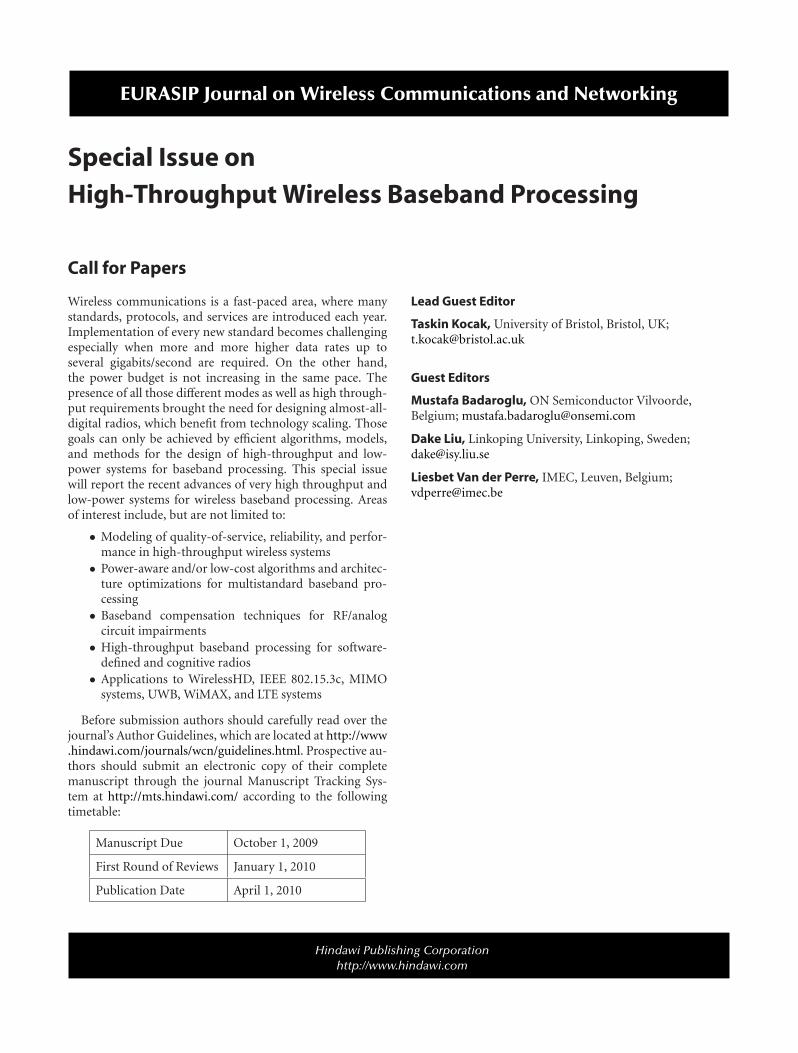
EURASIP Journal on Wireless Communications and Networking

Special Issue on

High-Throughput Wireless Baseband Processing

Call for Papers

Wireless communications is a fast-paced area, where manystandards, protocols, and services are introduced each year.Implementation of every new standard becomes challengingespecially when more and more higher data rates up toseveral gigabits/second are required. On the other hand,the power budget is not increasing in the same pace. Thepresence of all those different modes as well as high through-put requirements brought the need for designing almost-all-digital radios, which benefit from technology scaling. Thosegoals can only be achieved by efficient algorithms, models,and methods for the design of high-throughput and low-power systems for baseband processing. This special issuewill report the recent advances of very high throughput andlow-power systems for wireless baseband processing. Areasof interest include, but are not limited to:

• Modeling of quality-of-service, reliability, and perfor-mance in high-throughput wireless systems

• Power-aware and/or low-cost algorithms and architec-ture optimizations for multistandard baseband pro-cessing

• Baseband compensation techniques for RF/analogcircuit impairments

• High-throughput baseband processing for software-defined and cognitive radios

• Applications to WirelessHD, IEEE 802.15.3c, MIMOsystems, UWB, WiMAX, and LTE systems

Before submission authors should carefully read over thejournal’s Author Guidelines, which are located at http://www.hindawi.com/journals/wcn/guidelines.html. Prospective au-thors should submit an electronic copy of their completemanuscript through the journal Manuscript Tracking Sys-tem at http://mts.hindawi.com/ according to the followingtimetable:

Manuscript Due October 1, 2009

First Round of Reviews January 1, 2010

Publication Date April 1, 2010

Lead Guest Editor

Taskin Kocak, University of Bristol, Bristol, UK;[email protected]

Guest Editors

Mustafa Badaroglu, ON Semiconductor Vilvoorde,Belgium; [email protected]

Dake Liu, Linkoping University, Linkoping, Sweden;[email protected]

Liesbet Van der Perre, IMEC, Leuven, Belgium;[email protected]

Hindawi Publishing Corporationhttp://www.hindawi.com

http://www.hindawi.com/journals/wcn/guidelines.html


http://mts.hindawi.com/

mailto:[email protected]





Special Issue on

Simulators and Experimental Testbeds Design andDevelopment for Wireless Networks

Call for Papers

In the context of wireless networking, performance eval-uation of protocols and distributed applications is gen-erally conducted through simulation or experimentationcampaigns. An efficient and accurate simulation of wirelessnetworks raises various issues which generally need to beaddressed from several research domains simultaneously. Asexamples, we can consider the wireless physical layer mod-eling and simulation, the support of large-scale networks,the simulation of complex RF systems such as MIMO ones,the emulation of wireless nodes or the interconnection ofsimulators, experimental testbeds, and so forth.

The aim of this Special Issue is to bring together academicand industry researchers and practitioners from both thewireless networking and the simulation communities todiscuss current and future trends in simulation or experi-mentation techniques, models, and practices for the futurecommunication system and to foster interdisciplinary col-laborative research in this area. The guest editors seek high-quality papers on aspects of wireless network simulation, andvalue both theoretical and practical research contributions.Topics of interest include, but are not limited to:

• Radio medium modeling and cross-layer simulation

• Scalability, large-scale networks support

• Validation of simulators and simulation results

• Simulators benchmarking and comparisons

• Fluid-flow simulation for assessing QoS in large-scalenetworks

• Support of new emerging technologies (WiMax, 3.5G,Wireless Mesh Networks, 802.11x, etc.) in simulators

• Support of advanced RF systems (Multi-carrier sche-mes, MIMO, smart-antenna) in simulators

• Wireless node simulation or emulation

• Interoperability of simulators, emulators, and experi-ments

• Support of distributed physical layer schemes (dis-tributed signal processing; cooperative schemes)

• Distributed simulation, and scalability of simulators

• Implementation of simulators

• Experimental testbeds for wireless networks

• Methodology for protocol and distributed applicationperformance evaluation

• SDR techniques, cognitive radio approaches, dynamicspectrum access testbeds, and simulators as well asmodeling

• Simulation and testbeds for cooperative communica-tion protocols

Before submission, authors should carefully read over thejournal’s Author Guidelines, which are located at http://www.hindawi.com/journals/wcn/guidelines.html. Prospective au-thors should submit an electronic copy of their completemanuscript through the journal Manuscript Tracking Sys-tem at http://mts.hindawi.com/, according to the followingtimetable:

Manuscript Due June 1, 2009

First Round of Reviews September 1, 2009

Publication Date December 1, 2009

Lead Guest Editor

Faouzi Bader, Centre Tecnológico de Telecomunicacionesde Cataluya (CTTC), PMT, Spain; [email protected]

Guest Editors

Guillame Chelius, Institut National de Recherche enInformatique et en Automatique (INRA), France;[email protected]

Christian Ibars, Centre Tecnológico de Telecomunicacionesde Cataluya (CTTC), PMT, Spain; [email protected]

Mohamed Ibnkahla, Department of Electrical andComputer Engineering, Queen’s University, Canada;[email protected]

Nikos Passas, Department of Informatics andTelecommunications, University of Athens, Greece;[email protected]

Arnd-Ragnar Rhiemeier, Defence Electronics, EADSDeutschland GmbH, Germany;[email protected]












Special Issue on

Interference Management in Wireless CommunicationSystems: Theory and Applications

Call for Papers

Interference is a fundamental nature of wireless commu-nication systems, in which multiple transmissions oftentake place simultaneously over a common communicationmedium. In recent years, there has been a rapidly growinginterest in developing reliable and spectral efficient wirelesscommunication systems. One primary challenge in such adevelopment is how to deal with the interference, whichmay substantially limit the reliability and the throughputof a wireless communication system. In most existingwireless communication systems, interference is dealt withby coordinating users to orthogonalize their transmissionsin time or frequency, or by increasing transmission powerand treating each other’s interference as noise. Over the pasttwenty years, a number of sophisticated receiver designs,for example, multiuser detection, have been proposed forinterference suppression under various settings. Recently,the paradigm has shifted to focus on how to intelligentlyexploit the knowledge and/or the structure of interferenceto achieve improved reliability and throughput of wirelesscommunication systems.

This special issue aims to bring together state-of-the-artresearch contributions and practical implementations thateffectively manage interference in wireless communicationsystems. Original contributions in all areas related to inter-ference management for wireless communication systems aresolicited for this special issue. We are particularly interestedin manuscripts that report the latest development on inter-ference channels or cognitive radio channels from the per-spectives of information theory, signal processing, and cod-ing theory. Topics of interest include, but are not limited to:

• Information theoretic study of interference channelsor cognitive radio channels

• Game theoretical approach to interference manage-ment in wireless networks

• Cooperative wireless communication systems

• Relaying in interference networks• Advanced coding schemes for interference/cognitive

radio channels• Interference channels with confidentiality requirement• Femtocell networks

• Signal processing algorithms for interference mitigation• Receiver designs for interference channels or cognitive

radio channels• MIMO interference channels or MIMO cognitive

radio channels• Base station cooperation for interference mitigation• Network coding for interference channels or cognitive

radio channels• Resource allocation for interference management

Before submission authors should carefully read over thejournal’s Author Guidelines, which are located at http://www.hindawi.com/journals/wcn/guidelines.html. Prospective au-thors should submit an electronic copy of their completemanuscript through the journal Manuscript Tracking Sys-tem at http://mts.hindawi.com/ according to the followingtimetable:

Manuscript Due November 1, 2009

First Round of Reviews February 1, 2010

Publication Date June 1, 2010

Lead Guest Editor

Yan Xin, NEC Laboratories America, Inc., Princeton, NJ08540, USA; [email protected]

Guest Editors

Xiaodong Wang, Electrical Engineering Department,Columbia University, New York, NY 10027, USA;[email protected]

Geert Leus, Faculty of Electrical Engineering, Mathematicsand Computer Science, Delft University of Technology,Mekelweg 4, 2628 CD Delft, The Netherlands;[email protected]

Guosen Yue, NEC Laboratories America, Inc., Princeton,NJ 08540, USA; [email protected]

Jinhua Jiang, Department of Electrical Engineering,Stanford University Stanford, CA 94305, USA;[email protected]










an overview of the coding standard mpeg-4 audio … · eurasip journal on audio, speech, ... 2dolby...

Documents