An Optimizing Code Generator for a Class ofLattice-Boltzmann Computations

A THESIS

SUBMITTED FOR THE DEGREE OF

Master of Science (Engineering)

IN COMPUTER SCIENCE AND ENGINEERING

by

Irshad Muhammed Pananilath

Computer Science and Automation

Indian Institute of Science

BANGALORE – 560 012

JULY 2014

c©Irshad Muhammed Pananilath

JULY 2014

All rights reserved

TO

My Friends & Family

Acknowledgements

Apart from one’s efforts, the success of any project depends largely on the encouragement

and guidelines of many others. I would like to express my sincere appreciation and grat-

itude to my research advisor Prof. Dr. Uday Bondhugula who has been a tremendous

mentor to me. His patience and support has helped me overcome many crisis situations

and finish this dissertation.

I am also indebted to the members of the Multi-core Computing Lab - Aravind, Vinayaka,

Chandan, Roshan, Thejas, Somashekar, Ravi, and Vinay with whom I have interacted

closely during the course of my graduate studies. The many valuable discussions with

them helped me understand my research area better. A special thanks to Vinayaka and

Aravind for the close collaboration and for being there to bounce ideas with.

I have been very fortunate to make some wonderful friendships at IISc. I would always

cherish the beautiful times (the birthday celebrations, outings, treks and adventures) with

my group of friends, lovingly referred to as The Sanga. Anil Das and Remitha require special

mention for their hospitality and encouragement.

The institute and Dept. of CSA has provided all the facilities to make my stay here a

comfortable one. I am thankful to the office staff of CSA for taking care of the adminis-

trative tasks. Ministry of Human Resource Development has supported me throughout the

duration of the course with their scholarship.

I would also like to thank Anand Deshpande, Aniruddha Shet, Bharat Kaul, and Sunil

Sherlekar from Intel for the collaboration and joint work and also for providing us with

a Sandy Bridge system, Xeon Phi co-processor cards, and a license for the Intel Parallel

Studio Suite.

i

ii

Most importantly, none of this would have been possible without the love and patience

of my family. My wife, Munia has been really supportive throughout. I would also like to

extend my heart-felt gratitude to my brother, Dr. Fahad and my parents Dr. P Mohamed

and Dr. C Zeenath for their encouragement throughout this endeavor. I warmly appreciate

the understanding of my extended family.

Publications based on this Thesis

1. V. Bandishti, I. Pananilath, and U. Bondhugula. Tiling Stencil Computations to Maxi-

mize Parallelism, ACM/IEEE International Conference for High Performance Comput-

ing, Networking, Storage and Analysis (Supercomputing’12), Salt Lake City, Utah,

pages 40:1 - 40:11, November 2012.

2. I. Pananilath, A. Acharya, V. Vasista, and U. Bondhugula. An Optimizing Code Gener-

ator for a Class of Lattice-Boltzmann Computations, To be submitted.

iii

Abstract

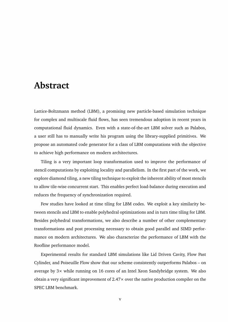
Lattice-Boltzmann method (LBM), a promising new particle-based simulation technique

for complex and multiscale fluid flows, has seen tremendous adoption in recent years in

computational fluid dynamics. Even with a state-of-the-art LBM solver such as Palabos,

a user still has to manually write his program using the library-supplied primitives. We

propose an automated code generator for a class of LBM computations with the objective

to achieve high performance on modern architectures.

Tiling is a very important loop transformation used to improve the performance of

stencil computations by exploiting locality and parallelism. In the first part of the work, we

explore diamond tiling, a new tiling technique to exploit the inherent ability of most stencils

to allow tile-wise concurrent start. This enables perfect load-balance during execution and

reduces the frequency of synchronization required.

Few studies have looked at time tiling for LBM codes. We exploit a key similarity be-

tween stencils and LBM to enable polyhedral optimizations and in turn time tiling for LBM.

Besides polyhedral transformations, we also describe a number of other complementary

transformations and post processing necessary to obtain good parallel and SIMD perfor-

mance on modern architectures. We also characterize the performance of LBM with the

Roofline performance model.

Experimental results for standard LBM simulations like Lid Driven Cavity, Flow Past

Cylinder, and Poiseuille Flow show that our scheme consistently outperforms Palabos – on

average by 3× while running on 16 cores of an Intel Xeon Sandybridge system. We also

obtain a very significant improvement of 2.47× over the native production compiler on the

SPEC LBM benchmark.

v

vi

Contents

Acknowledgements i

Publications based on this Thesis iii

Abstract v

1 Introduction 1

2 Lattice-Boltzmann Method 52.1 Lattice-Boltzmann Equation . . . . . . . . . . . . . . . . . . . . . . . . . . . . . . 62.2 Lattice Arrangements . . . . . . . . . . . . . . . . . . . . . . . . . . . . . . . . . . 62.3 Collision Models . . . . . . . . . . . . . . . . . . . . . . . . . . . . . . . . . . . . . 72.4 Boundary Conditions . . . . . . . . . . . . . . . . . . . . . . . . . . . . . . . . . . 82.5 Implementation Strategies . . . . . . . . . . . . . . . . . . . . . . . . . . . . . . 92.6 Data Layout . . . . . . . . . . . . . . . . . . . . . . . . . . . . . . . . . . . . . . . 11

3 Tiling Stencil Computations 133.1 Polyhedral Model . . . . . . . . . . . . . . . . . . . . . . . . . . . . . . . . . . . . 13

3.1.1 Iteration Spaces . . . . . . . . . . . . . . . . . . . . . . . . . . . . . . . . 143.1.2 Dependences . . . . . . . . . . . . . . . . . . . . . . . . . . . . . . . . . . 143.1.3 Hyperplanes . . . . . . . . . . . . . . . . . . . . . . . . . . . . . . . . . . . 15

3.2 Tiling . . . . . . . . . . . . . . . . . . . . . . . . . . . . . . . . . . . . . . . . . . . 153.2.1 Validity of Tiling . . . . . . . . . . . . . . . . . . . . . . . . . . . . . . . . 163.2.2 Time Tiling . . . . . . . . . . . . . . . . . . . . . . . . . . . . . . . . . . . 17

3.3 Pipelined Vs Concurrent Start . . . . . . . . . . . . . . . . . . . . . . . . . . . . 193.4 Diamond Tiling . . . . . . . . . . . . . . . . . . . . . . . . . . . . . . . . . . . . . 20

4 Our LBM Optimization Framework 234.1 System Overview . . . . . . . . . . . . . . . . . . . . . . . . . . . . . . . . . . . . 234.2 Design Decisions . . . . . . . . . . . . . . . . . . . . . . . . . . . . . . . . . . . . . 244.3 Polyhedral Representation for LBM in a DSL . . . . . . . . . . . . . . . . . . . 264.4 Complementary Optimizations . . . . . . . . . . . . . . . . . . . . . . . . . . . . 27

4.4.1 Simplification of the LBM Kernel . . . . . . . . . . . . . . . . . . . . . . 284.4.2 Eliminating Modulos from the Inner Kernel . . . . . . . . . . . . . . . 284.4.3 Boundary Tile Separation . . . . . . . . . . . . . . . . . . . . . . . . . . 28

vii

viii CONTENTS

4.4.4 Data Alignment . . . . . . . . . . . . . . . . . . . . . . . . . . . . . . . . . 294.4.5 Inlining & Unrolling . . . . . . . . . . . . . . . . . . . . . . . . . . . . . . 304.4.6 Predicated SIMDization . . . . . . . . . . . . . . . . . . . . . . . . . . . . 304.4.7 Memory Optimization . . . . . . . . . . . . . . . . . . . . . . . . . . . . . 304.4.8 Tile Sizes . . . . . . . . . . . . . . . . . . . . . . . . . . . . . . . . . . . . . 31

5 Experimental Evaluation 335.1 Experimental Setup . . . . . . . . . . . . . . . . . . . . . . . . . . . . . . . . . . . 335.2 Benchmarks . . . . . . . . . . . . . . . . . . . . . . . . . . . . . . . . . . . . . . . 33

5.2.1 Lid Driven Cavity . . . . . . . . . . . . . . . . . . . . . . . . . . . . . . . . 345.2.2 SPEC LBM . . . . . . . . . . . . . . . . . . . . . . . . . . . . . . . . . . . . 345.2.3 Poiseuille Flow . . . . . . . . . . . . . . . . . . . . . . . . . . . . . . . . . 355.2.4 Flow Past Cylinder . . . . . . . . . . . . . . . . . . . . . . . . . . . . . . . 355.2.5 MRT – GLBM . . . . . . . . . . . . . . . . . . . . . . . . . . . . . . . . . . 36

5.3 Performance Metrics . . . . . . . . . . . . . . . . . . . . . . . . . . . . . . . . . . 365.4 Performance Modeling with Roofline Model . . . . . . . . . . . . . . . . . . . . 375.5 Performance Analysis . . . . . . . . . . . . . . . . . . . . . . . . . . . . . . . . . . 39

6 Related Work 43

7 Conclusions 49

Bibliography 51

List of Tables

5.1 Architecture details . . . . . . . . . . . . . . . . . . . . . . . . . . . . . . . . . . . 345.2 Problem sizes used for the benchmarks . . . . . . . . . . . . . . . . . . . . . . . 35

ix

List of Figures

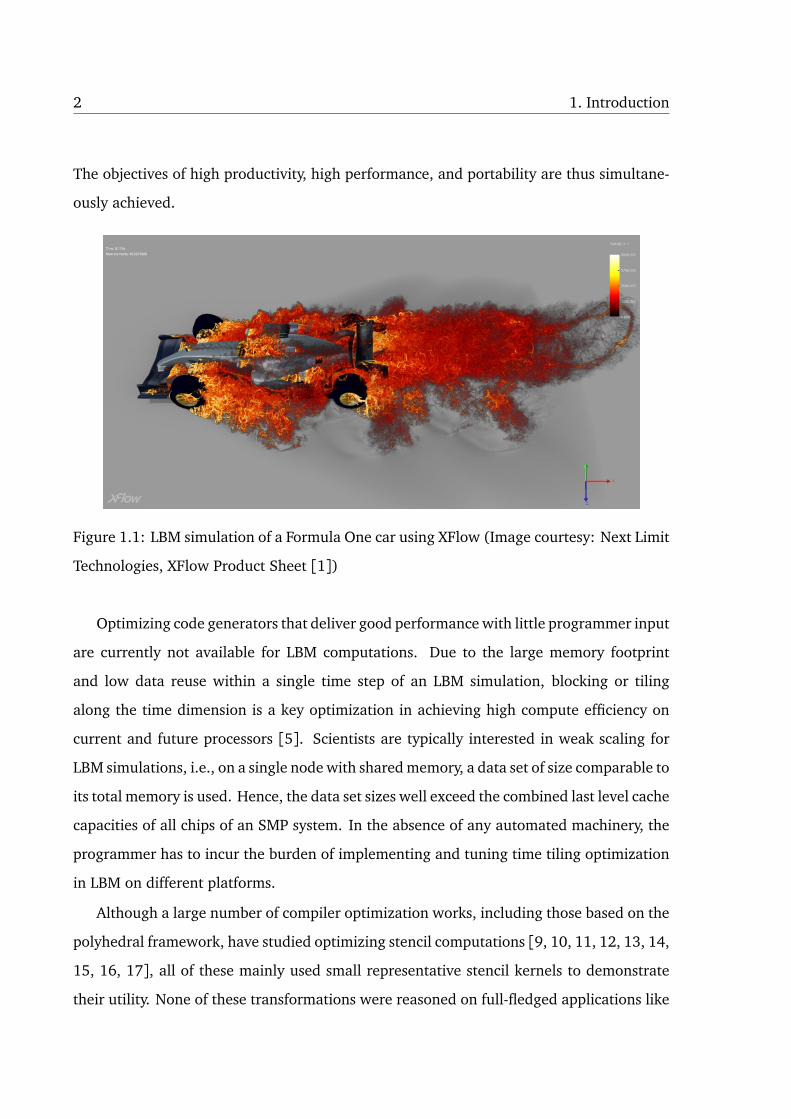
1.1 LBM simulation of a Formula One car using XFlow (Image courtesy: NextLimit Technologies, XFlow Product Sheet [1]) . . . . . . . . . . . . . . . . . . 2

1.2 Lid Driven Cavity & Flow Past Cylinder LBM simulations . . . . . . . . . . . . 3

2.1 D2Q9 (left) & D3Q19 (right) lattice arrangements . . . . . . . . . . . . . . . . 72.2 Unknown PDFs on all 4 boundaries . . . . . . . . . . . . . . . . . . . . . . . . . 82.3 Illustration of Bounce Back BC . . . . . . . . . . . . . . . . . . . . . . . . . . . . 92.4 Typical LBM algorithm . . . . . . . . . . . . . . . . . . . . . . . . . . . . . . . . . 102.5 LBM - Push model for D2Q9 lattice . . . . . . . . . . . . . . . . . . . . . . . . . 102.6 LBM - Pull model for D2Q9 lattice . . . . . . . . . . . . . . . . . . . . . . . . . . 11

3.1 Representation in the polyhedral model . . . . . . . . . . . . . . . . . . . . . . 143.2 Tiling an iteration space . . . . . . . . . . . . . . . . . . . . . . . . . . . . . . . . 163.3 Pipelined start . . . . . . . . . . . . . . . . . . . . . . . . . . . . . . . . . . . . . . 193.4 Concurrent start . . . . . . . . . . . . . . . . . . . . . . . . . . . . . . . . . . . . . 203.5 Tile shape for a 2-d LBM (d2q9 for example); arrows represent hyperplanes. 21

4.1 msLBM overview . . . . . . . . . . . . . . . . . . . . . . . . . . . . . . . . . . . . 234.2 Illustrative 1-d LBM with single grid . . . . . . . . . . . . . . . . . . . . . . . . 254.3 1-d stencil . . . . . . . . . . . . . . . . . . . . . . . . . . . . . . . . . . . . . . . . . 264.4 Illustrative example - Pull scheme on a 1-d LBM . . . . . . . . . . . . . . . . . 274.5 Modulo hoisting example . . . . . . . . . . . . . . . . . . . . . . . . . . . . . . . 294.6 Predicated SIMD example . . . . . . . . . . . . . . . . . . . . . . . . . . . . . . . 30

5.1 Setting for a 2-d LDC simulation . . . . . . . . . . . . . . . . . . . . . . . . . . . 365.2 2-d Poiseuille flow setting . . . . . . . . . . . . . . . . . . . . . . . . . . . . . . . 375.3 Roofline model with ceiling for LBM (logarithmic scales are used on both

axes) . . . . . . . . . . . . . . . . . . . . . . . . . . . . . . . . . . . . . . . . . . . . 385.4 Performance on Intel Xeon (Sandybridge) . . . . . . . . . . . . . . . . . . . . . 405.5 Comparison of MEUPS across benchmarks for mslbm . . . . . . . . . . . . . . 41

6.1 Compressed Grid technique [2] . . . . . . . . . . . . . . . . . . . . . . . . . . . 446.2 2-d blocking (4x4 blocking factor) by Wilke et al. [2] . . . . . . . . . . . . . . 456.3 COLBA - The mapping of virtually decomposed domains to a tree [3, 4] . . 466.4 3.5d blocking [5] . . . . . . . . . . . . . . . . . . . . . . . . . . . . . . . . . . . . 46

xi

Chapter 1

Introduction

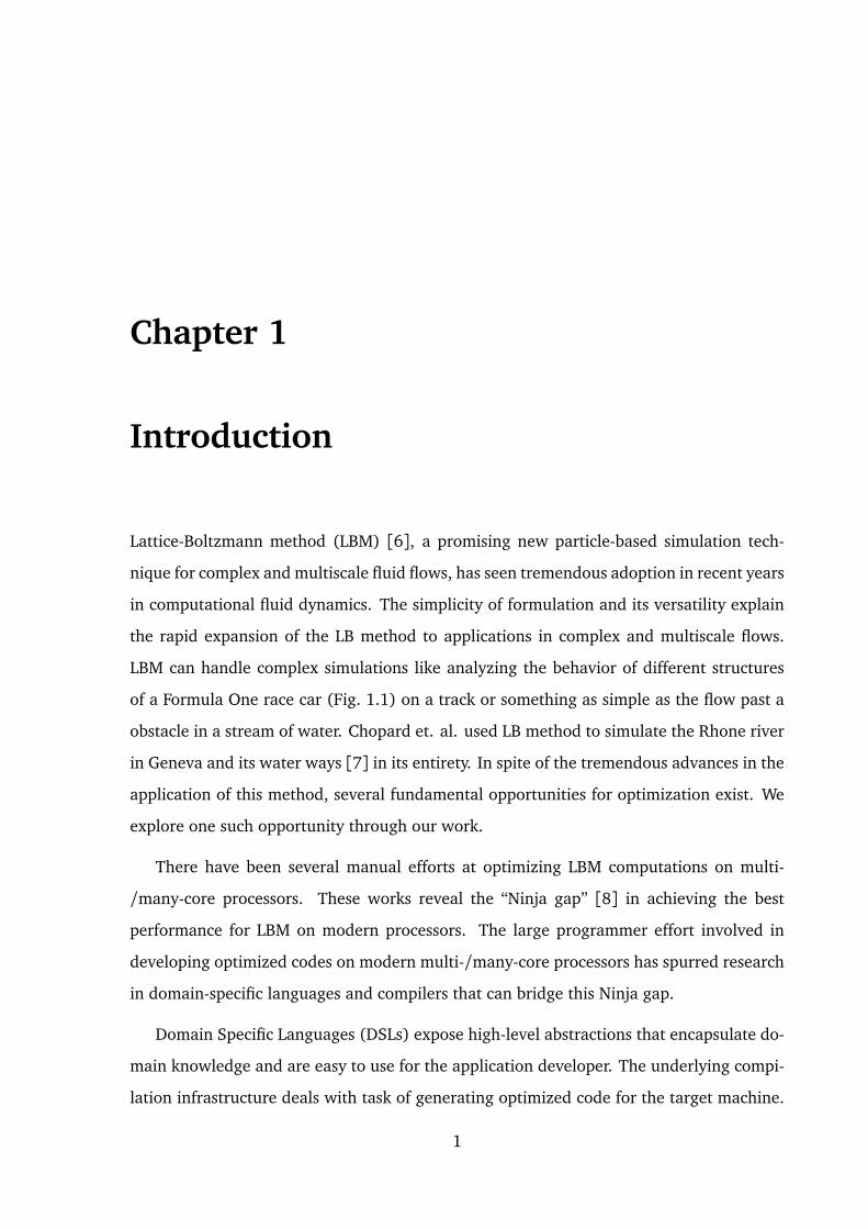
Lattice-Boltzmann method (LBM) [6], a promising new particle-based simulation tech-

nique for complex and multiscale fluid flows, has seen tremendous adoption in recent years

in computational fluid dynamics. The simplicity of formulation and its versatility explain

the rapid expansion of the LB method to applications in complex and multiscale flows.

LBM can handle complex simulations like analyzing the behavior of different structures

of a Formula One race car (Fig. 1.1) on a track or something as simple as the flow past a

obstacle in a stream of water. Chopard et. al. used LB method to simulate the Rhone river

in Geneva and its water ways [7] in its entirety. In spite of the tremendous advances in the

application of this method, several fundamental opportunities for optimization exist. We

explore one such opportunity through our work.

There have been several manual efforts at optimizing LBM computations on multi-

/many-core processors. These works reveal the “Ninja gap” [8] in achieving the best

performance for LBM on modern processors. The large programmer effort involved in

developing optimized codes on modern multi-/many-core processors has spurred research

in domain-specific languages and compilers that can bridge this Ninja gap.

Domain Specific Languages (DSLs) expose high-level abstractions that encapsulate do-

main knowledge and are easy to use for the application developer. The underlying compi-

lation infrastructure deals with task of generating optimized code for the target machine.

1

2 1. Introduction

The objectives of high productivity, high performance, and portability are thus simultane-

ously achieved.

Figure 1.1: LBM simulation of a Formula One car using XFlow (Image courtesy: Next Limit

Technologies, XFlow Product Sheet [1])

Optimizing code generators that deliver good performance with little programmer input

are currently not available for LBM computations. Due to the large memory footprint

and low data reuse within a single time step of an LBM simulation, blocking or tiling

along the time dimension is a key optimization in achieving high compute efficiency on

current and future processors [5]. Scientists are typically interested in weak scaling for

LBM simulations, i.e., on a single node with shared memory, a data set of size comparable to

its total memory is used. Hence, the data set sizes well exceed the combined last level cache

capacities of all chips of an SMP system. In the absence of any automated machinery, the

programmer has to incur the burden of implementing and tuning time tiling optimization

in LBM on different platforms.

Although a large number of compiler optimization works, including those based on the

polyhedral framework, have studied optimizing stencil computations [9, 10, 11, 12, 13, 14,

15, 16, 17], all of these mainly used small representative stencil kernels to demonstrate

their utility. None of these transformations were reasoned on full-fledged applications like

3

LBM. LBM computations exhibit near-neighbor interactions conceptually similar to those

representative stencils, and potentially very different arithmetic intensities and underlying

data structures. On the other hand, recent works that did study optimizing LBM have been

manual efforts [5, 18]. Library-based approaches and LBM solvers like Palabos [19] still

require users to manually write LBM simulations using library-supplied primitives. Though

this improves productivity, obtaining high performance is elusive as our evaluation later

demonstrates.

Through this work, we propose an optimizing code generator for a class of LBM com-

putations focusing on time tiling and polyhedral optimizations to enable time tiling in LBM

where the choice of data structure and compute intensity could potentially affect the ability

to optimize and the resulting gains. We employ diamond tiling [15], a new tiling technique

to exploit the inherent ability of most stencils to allow tile-wise concurrent start. This en-

ables perfect load-balance during execution and reduces the frequency of synchronizations

required in addition to the cache locality and parallelization benefits of tiling.

(a) Lid Driven Cavity (b) Flow Past Cylinder

Figure 1.2: Lid Driven Cavity & Flow Past Cylinder LBM simulations

Our optimization process exploits a key similarity between stencils and LBM to enable

polyhedral compiler optimizations and in turn time blocking for LBM. We demonstrate the

effectiveness of our approach on the SPEC LBM benchmark and LBM simulations like Lid

Driven Cavity [20] (Fig. 1.2a), Flow Past Cylinder [21] (Fig. 1.2b), Poiseuille Flow [22]

on an Intel Xeon SMP based on the Sandybridge microarchitecture. To the best of our

4 1. Introduction

knowledge, this is the first work that enables and integrates automatic polyhedral opti-

mizations for LBM computations. Besides polyhedral transformations, we also describe a

number of other complementary transformations and post processing necessary to obtain

good parallel and SIMD performance.

The class of LBM simulations that we handle are those that do not involve moving

obstacles or periodic data grids. Periodic data grids along with periodic boundary condi-

tions are used to model large (infinite) systems using a small portion. The domain wraps

around along the dimensions that are periodic and the points at both the boundaries be-

come neighbors resulting in cyclic dependences. The techniques and optimizations we

study are also conceptually applicable to other classes of LBM as well, but an additional

non-trivial amount of work is needed to handle those.

The roofline model [23] relates performance of kernels to the architecture’s character-

istics and can often provide insights into bottlenecks and tuning. In particular, one can

determine if an execution is memory bandwidth bound, computation bound, or neither.

We present the roofline analysis for a 2-d (mrt-d2q9) and a 3-d (ldc-d3q27) LBM kernel

and conclude that msLBM obtains further improvement over Palabos in both operational

intensity and peak achievable performance.

Experimental results for standard LBM simulations like Lid Driven Cavity, Flow Past

Cylinder, and Poiseuille Flow show that our scheme consistently outperforms Palabos – on

average by 3× while running on 16 cores of an Intel Xeon Sandybridge system. We also

obtain a very significant improvement of 2.47× over the native production compiler on the

SPEC LBM benchmark.

The rest of this thesis is organized as follows. Chapter 2 provides background on LBM.

Chapter 3 describes the polyhedral framework and our work on improving tiling techniques

for parallelism. Chapter 4 describes the optimization process integrated into our code

generator. Chapter 5 presents experimental results, Chapter 6 outlines the related work

and conclusions are presented in Chapter 7.

Chapter 2

Lattice-Boltzmann Method

In this chapter, we review the basics of the Lattice-Boltzmann method. The Lattice-Boltzmann

method has its origins in the Lattice Gas Automata (LGA) theory and is being increasingly

used for simulation of complex fluid flows [24] in computational fluid dynamics. For the

purposes of optimization, only the nature of dependences and computation need to be

understood by a reader.

Generally, simulations can be performed at multiple scales. On a macroscopic scale,

partial differential equations like the Navier-Stokes equation are used. Since it is very

difficult to solve them analytically, an iterative technique is used where the simulation is

carried out until satisfying results are obtained. The second approach is to simulate small

particles on a microscopic scale and then derive the macroscopic quantities of interest from

them. But there would be simply too much data to handle in order to simulate a problem

that is interesting on a macroscopic scale.

The Lattice-Boltzmann method closes the gap between macro-scale and micro-scale.

The crux of Lattice-Boltzmann method is the construction of simple kinetic models that

capture the essential physics of microscopic processes such that the averaged macroscopic

properties follow the corresponding laws at the macroscopic scale.

5

6 2. Lattice-Boltzmann Method

2.1 Lattice-Boltzmann Equation

The Lattice-Boltzmann equation is a discretized form of the Boltzmann equation with the

quantities time, space and momentum being discretized. In LBM, fluid flows are modeled

as hypothetical particles moving in a discretized lattice domain (space) with different lat-

tice velocities (discretized momentum) over different time steps (discretized time). Eq. 2.1

shows the discretized form of Lattice-Boltzmann equation, where fi is the particle distri-

bution function (PDF) along the i th direction, ∆t is the time increment, Ωi is the collision

operator and n is the number of PDFs based on the lattice used.

fi(x+ ci∆t, t +∆t) = fi(x, t) +Ωi( fi(x, t)), i = 0, . . . n. (2.1)

This equation is usually solved in two steps, the collision step (Eq. 2.2) and the advection

step (Eq. 2.3).

f ∗i (x, t +∆t) = fi(x, t) +Ωi( fi(x, t)) (2.2)

fi(x+ ci∆t, t +∆t) = f ∗i (x, t +∆t) (2.3)

The collision step models the interaction among the particles that arrive at a lattice node.

It is clear from Eqn. 2.2 that the collision step only involves quantities that are local to a

particular node. The advection step, captures the movement of particles to the neighboring

nodes of the lattice along the velocity directions dictated by the lattice arrangement used.

In short, Lattice-Boltzmann equation describes the evolution of a set of particles on a lattice

through collision and advection.

2.2 Lattice Arrangements

The set of allowed velocities in the Lattice-Boltzmann models is restricted by conservation

of mass and momentum, and by rotational symmetry.

2.3. Collision Models 7

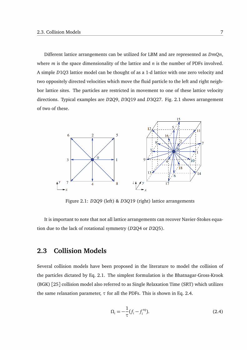
Different lattice arrangements can be utilized for LBM and are represented as DmQn,

where m is the space dimensionality of the lattice and n is the number of PDFs involved.

A simple D1Q3 lattice model can be thought of as a 1-d lattice with one zero velocity and

two oppositely directed velocities which move the fluid particle to the left and right neigh-

bor lattice sites. The particles are restricted in movement to one of these lattice velocity

directions. Typical examples are D2Q9, D3Q19 and D3Q27. Fig. 2.1 shows arrangement

of two of these.

Figure 2.1: D2Q9 (left) & D3Q19 (right) lattice arrangements

It is important to note that not all lattice arrangements can recover Navier-Stokes equa-

tion due to the lack of rotational symmetry (D2Q4 or D2Q5).

2.3 Collision Models

Several collision models have been proposed in the literature to model the collision of

the particles dictated by Eq. 2.1. The simplest formulation is the Bhatnagar-Gross-Krook

(BGK) [25] collision model also referred to as Single Relaxation Time (SRT) which utilizes

the same relaxation parameter, τ for all the PDFs. This is shown in Eq. 2.4.

Ωi = −1τ( fi − f eq

i ). (2.4)

8 2. Lattice-Boltzmann Method

Even though BGK collision model is the most popular choice because of its simplicity,

it suffers from instability issues for low viscosity fluids.

Multiple Relaxation Time (MRT) collision model given in Eq. 2.5, proposed by d’Humières [26],

uses a collision matrix to relax the PDFs towards their local equilibria. It doesn’t suffer from

the afore mentioned stability issues. Substituting S with 1τI, where I is an identity matrix,

recovers the BGK model from MRT.

~Ω= −S( ~f − ~f eq) (2.5)

The choice of collision model affects the arithmetic intensity of the LBM kernel.

2.4 Boundary Conditions

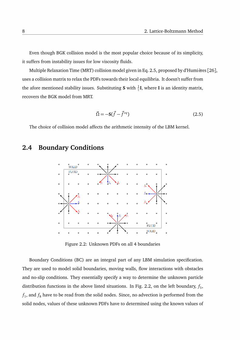
Figure 2.2: Unknown PDFs on all 4 boundaries

Boundary Conditions (BC) are an integral part of any LBM simulation specification.

They are used to model solid boundaries, moving walls, flow interactions with obstacles

and no-slip conditions. They essentially specify a way to determine the unknown particle

distribution functions in the above listed situations. In Fig. 2.2, on the left boundary, f5,

f1, and f8 have to be read from the solid nodes. Since, no advection is performed from the

solid nodes, values of these unknown PDFs have to determined using the known values of

2.5. Implementation Strategies 9

the particular fluid node.

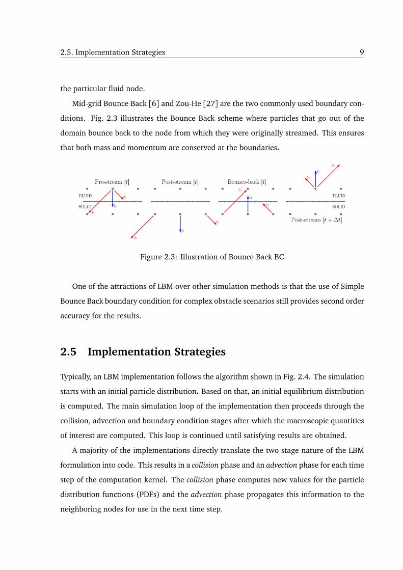
Mid-grid Bounce Back [6] and Zou-He [27] are the two commonly used boundary con-

ditions. Fig. 2.3 illustrates the Bounce Back scheme where particles that go out of the

domain bounce back to the node from which they were originally streamed. This ensures

that both mass and momentum are conserved at the boundaries.

Figure 2.3: Illustration of Bounce Back BC

One of the attractions of LBM over other simulation methods is that the use of Simple

Bounce Back boundary condition for complex obstacle scenarios still provides second order

accuracy for the results.

2.5 Implementation Strategies

Typically, an LBM implementation follows the algorithm shown in Fig. 2.4. The simulation

starts with an initial particle distribution. Based on that, an initial equilibrium distribution

is computed. The main simulation loop of the implementation then proceeds through the

collision, advection and boundary condition stages after which the macroscopic quantities

of interest are computed. This loop is continued until satisfying results are obtained.

A majority of the implementations directly translate the two stage nature of the LBM

formulation into code. This results in a collision phase and an advection phase for each time

step of the computation kernel. The collision phase computes new values for the particle

distribution functions (PDFs) and the advection phase propagates this information to the

neighboring nodes for use in the next time step.

10 2. Lattice-Boltzmann Method

Initialize Collision

Advection

BoundaryConditions

MacroscopicQuantities Result

Figure 2.4: Typical LBM algorithm

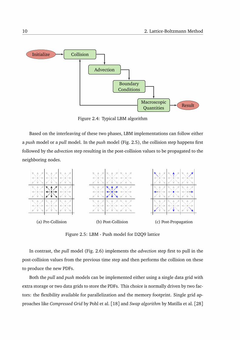
Based on the interleaving of these two phases, LBM implementations can follow either

a push model or a pull model. In the push model (Fig. 2.5), the collision step happens first

followed by the advection step resulting in the post-collision values to be propagated to the

neighboring nodes.

(a) Pre-Collision (b) Post-Collision (c) Post-Propagation

Figure 2.5: LBM - Push model for D2Q9 lattice

In contrast, the pull model (Fig. 2.6) implements the advection step first to pull in the

post-collision values from the previous time step and then performs the collision on these

to produce the new PDFs.

Both the pull and push models can be implemented either using a single data grid with

extra storage or two data grids to store the PDFs. This choice is normally driven by two fac-

tors: the flexibility available for parallelization and the memory footprint. Single grid ap-

proaches like Compressed Grid by Pohl et al. [18] and Swap algorithm by Matilla et al. [28]

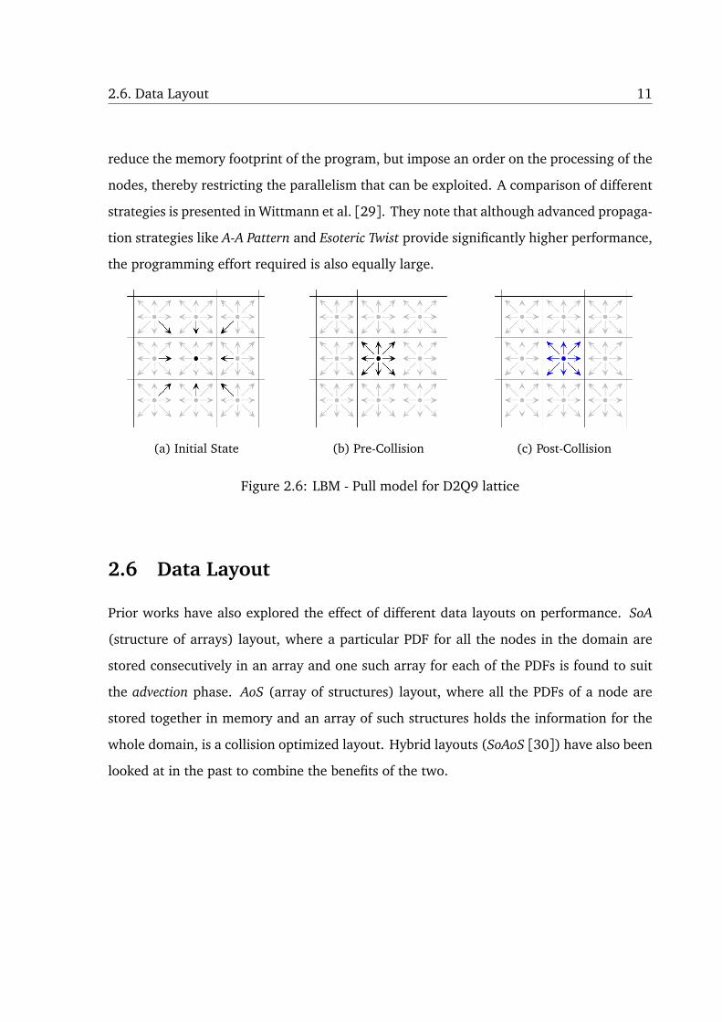
2.6. Data Layout 11

reduce the memory footprint of the program, but impose an order on the processing of the

nodes, thereby restricting the parallelism that can be exploited. A comparison of different

strategies is presented in Wittmann et al. [29]. They note that although advanced propaga-

tion strategies like A-A Pattern and Esoteric Twist provide significantly higher performance,

the programming effort required is also equally large.

(a) Initial State (b) Pre-Collision (c) Post-Collision

Figure 2.6: LBM - Pull model for D2Q9 lattice

2.6 Data Layout

Prior works have also explored the effect of different data layouts on performance. SoA

(structure of arrays) layout, where a particular PDF for all the nodes in the domain are

stored consecutively in an array and one such array for each of the PDFs is found to suit

the advection phase. AoS (array of structures) layout, where all the PDFs of a node are

stored together in memory and an array of such structures holds the information for the

whole domain, is a collision optimized layout. Hybrid layouts (SoAoS [30]) have also been

looked at in the past to combine the benefits of the two.

Chapter 3

Tiling Stencil Computations

In this chapter, we explain the concepts of the polyhedral model and loop tiling as a poly-

hedral transformation. We also also expand on the need for diamond tiling, its benefits

and the necessary and sufficient conditions for performing diamond tiling.

3.1 Polyhedral Model

The Polyhedral Model [31] is a mathematical framework for compiler optimization based

on parametric integer linear programming and linear algebra. It provides a high-level

representation for loop nests and the associated dependences in a program using integer

points in a polyhedra. The dynamic instances of the statements in the program that are

surrounded by loop nests become the integer points inside the polyhedra.

The polyhedral model is applicable to loop nests in which the data access functions and

loop bounds are affine combinations (linear combination with a constant) of the enclosing

loop variables and parameters. Affine transformations can then be used to reason about

complex execution reorderings that can improve locality and parallelism. With several re-

cent advances, the polyhedral model has reached a level of maturity in various aspects - in

particular as a powerful intermediate representation for performing powerful transforma-

tions, and code generation after transformations.

13

14 3. Tiling Stencil Computations

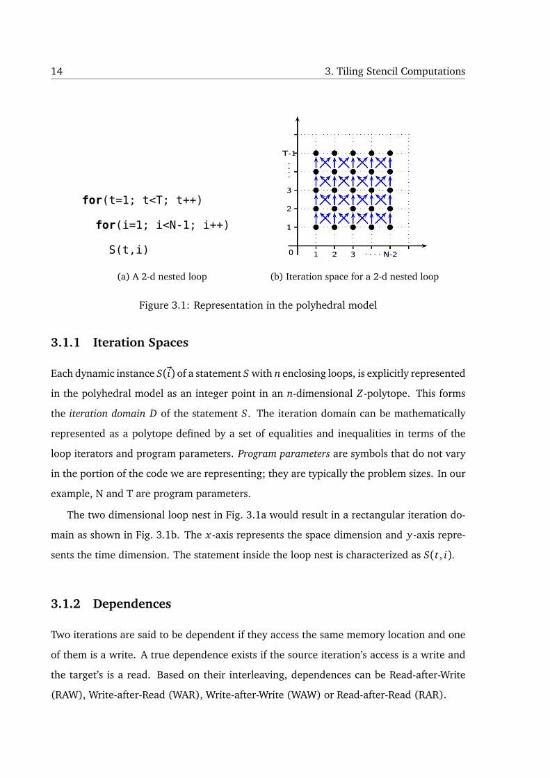
for(t=1; t<T; t++)

for(i=1; i<N-1; i++)

S(t,i)

(a) A 2-d nested loop (b) Iteration space for a 2-d nested loop

Figure 3.1: Representation in the polyhedral model

3.1.1 Iteration Spaces

Each dynamic instance S(~i) of a statement S with n enclosing loops, is explicitly represented

in the polyhedral model as an integer point in an n-dimensional Z-polytope. This forms

the iteration domain D of the statement S. The iteration domain can be mathematically

represented as a polytope defined by a set of equalities and inequalities in terms of the

loop iterators and program parameters. Program parameters are symbols that do not vary

in the portion of the code we are representing; they are typically the problem sizes. In our

example, N and T are program parameters.

The two dimensional loop nest in Fig. 3.1a would result in a rectangular iteration do-

main as shown in Fig. 3.1b. The x-axis represents the space dimension and y-axis repre-

sents the time dimension. The statement inside the loop nest is characterized as S(t, i).

3.1.2 Dependences

Two iterations are said to be dependent if they access the same memory location and one

of them is a write. A true dependence exists if the source iteration’s access is a write and

the target’s is a read. Based on their interleaving, dependences can be Read-after-Write

(RAW), Write-after-Read (WAR), Write-after-Write (WAW) or Read-after-Read (RAR).

3.2. Tiling 15

Dependences are an important concept while studying execution reordering since a

reordering will only be legal if does not violate the dependences, i.e., one is allowed to

change the order in which operations are performed as long as the transformed program

has the same execution order with respect to the dependent iterations. For the iteration

domain shown in Fig. 3.1b, the blue arrows show dependences. Each dynamic instance of

the statement S depends on three values from the previous time iteration.

3.1.3 Hyperplanes

A hyperplane is an n − 1 dimensional affine subspace of an n dimensional space. For

example, any line is a hyperplane in a 2-d space, and any 2-d plane is a hyperplane in 3-d

space.

A hyperplane for a statement Si is of the form:

φSi(~x) = h· ~x + h0 (3.1)

where h0 is the translation or the constant shift component, and ~x is an iteration of Si.

h itself can be viewed as a vector oriented in a direction normal to the hyperplane.

Hyperplanes can be interpreted as schedules, allocations, or partitions based on the

properties they satisfy. Saying that a hyperplane is one of them implies a particular prop-

erty that the new loop will satisfy in the transformed space. Based on the properties the

hyperplanes will satisfy at various levels, certain further transformations like tiling, unroll-

jamming, or marking it parallel, can be performed.

3.2 Tiling

Loop tiling is a key optimization often used to exploit cache locality and extract coarse-

grained parallelism. Tiling for locality requires grouping points in an iteration space into

smaller blocks (tiles) allowing reuse in multiple directions when the block fits in a faster

memory like registers or multiple levels of processor cache. Then execution proceeds tile

16 3. Tiling Stencil Computations

by tile, with each tile being executed atomically. Reuse distances are no longer a function

of the problem size, but a function of the tile size.

Tiling can be performed multiple times, once for each level of the memory hierarchy.

Tiling for coarse-grained parallelism involves partitioning the iteration space into tiles that

may be concurrently executed on different processors/cores with a reduced frequency and

volume of inter-processor communication: a tile is atomically executed on a processor with

communication required only before and after execution.

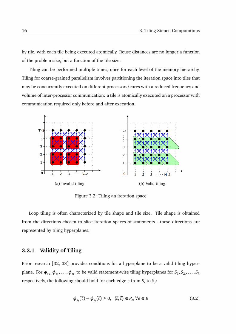
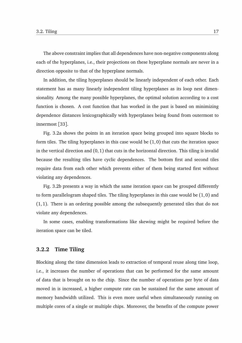
(a) Invalid tiling (b) Valid tiling

Figure 3.2: Tiling an iteration space

Loop tiling is often characterized by tile shape and tile size. Tile shape is obtained

from the directions chosen to slice iteration spaces of statements - these directions are

represented by tiling hyperplanes.

3.2.1 Validity of Tiling

Prior research [32, 33] provides conditions for a hyperplane to be a valid tiling hyper-

plane. For φs1,φs2

, . . . ,φskto be valid statement-wise tiling hyperplanes for S1, S2,, . . . , Sk

respectively, the following should hold for each edge e from Si to S j:

φs j(~t)−φsi

(~s)≥ 0, ⟨~s,~t⟩ ∈ Pe,∀e ∈ E (3.2)

3.2. Tiling 17

The above constraint implies that all dependences have non-negative components along

each of the hyperplanes, i.e., their projections on these hyperplane normals are never in a

direction opposite to that of the hyperplane normals.

In addition, the tiling hyperplanes should be linearly independent of each other. Each

statement has as many linearly independent tiling hyperplanes as its loop nest dimen-

sionality. Among the many possible hyperplanes, the optimal solution according to a cost

function is chosen. A cost function that has worked in the past is based on minimizing

dependence distances lexicographically with hyperplanes being found from outermost to

innermost [33].

Fig. 3.2a shows the points in an iteration space being grouped into square blocks to

form tiles. The tiling hyperplanes in this case would be (1,0) that cuts the iteration space

in the vertical direction and (0,1) that cuts in the horizontal direction. This tiling is invalid

because the resulting tiles have cyclic dependences. The bottom first and second tiles

require data from each other which prevents either of them being started first without

violating any dependences.

Fig. 3.2b presents a way in which the same iteration space can be grouped differently

to form parallelogram shaped tiles. The tiling hyperplanes in this case would be (1,0) and

(1, 1). There is an ordering possible among the subsequently generated tiles that do not

violate any dependences.

In some cases, enabling transformations like skewing might be required before the

iteration space can be tiled.

3.2.2 Time Tiling

Blocking along the time dimension leads to extraction of temporal reuse along time loop,

i.e., it increases the number of operations that can be performed for the same amount

of data that is brought on to the chip. Since the number of operations per byte of data

moved in is increased, a higher compute rate can be sustained for the same amount of

memory bandwidth utilized. This is even more useful when simultaneously running on

multiple cores of a single or multiple chips. Moreover, the benefits of the compute power

18 3. Tiling Stencil Computations

of a single chip via SIMDization are also seen when the data comes from the cache. A

simple calculation shows that the amount of bandwidth needed to keep the SIMD units is

prohibitively high when there is no cache reuse. The space loops of LBM, i.e., loops that

iterate over the data grid have limited (a constant factor) reuse. In particular, consider

d2q9, where there may be about 70-80 operations performed for every nine elements of

the grid. This ratio of operations to off-chip load/stores for the straightforward original

execution order is not sufficient to keep all compute units busy. This will also be supported

by experimental results presented later.

There are several time tiling techniques for stencils in the literature. It is well known

that straightforward rectangular tiling of stencils is not valid [34, 35]. One needs to skew

the space loops typically by a factor of one with respect to the time loop. Hence, the

most natural tiling technique has been to use (hyper-)parallelograms [34, 35, 9, 10]. This

is equivalent to skewing the space loops with respect to the time loop and performing

rectangular tiling. Parallelogram tiling suffers from pipelined startup and drain besides

limiting the amount of parallelism on the wavefront depending on the number of time steps

and time tile size. Another approach is to use overlapping trapezoids [11]. Such an overlap

not only leads to redundant computation, but more importantly makes code generation

very hard to automate – this is no automatic generator for it yet. Yet another approach is

to use a combination of trapezoids and inverted trapezoids as is done by Pochoir [36]with a

recursive cache oblivious technique. Eventhough, manual tiling of the iteration space using

diamond shaped tiles had been tried before by Orozco et al. [37] and Strzodka et al. [38],

the recently proposed automated diamond tiling technique [15] allowed concurrent start

in the tile space while not adding any additional complexity to code generation or any

redundant computation. We describe this in a little more detail in the next section. In depth

explanation of the theoretical formulation for diamond tiling can be found in Bandishti

et al. [15]. With diamond tiling having already been demonstrated as the simpler and

better performing one on modern multicores [15], we choose diamond tiling as the time

tiling scheme for LBM. Hexagonal tiling and hybrid tile shapes [39, 17] have recently been

proposed but their benefits for general purpose multicores are yet to be evaluated.

3.3. Pipelined Vs Concurrent Start 19

3.3 Pipelined Vs Concurrent Start

Performing parallelization and locality optimization together on stencils can often lead to

pipelined start-up, i.e., not all processors are busy during parallelized execution. This is

the case with a number of general compiler techniques from the literature [40, 41, 33].

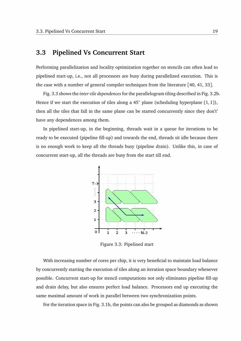
Fig. 3.3 shows the inter-tile dependences for the parallelogram tiling described in Fig. 3.2b.

Hence if we start the execution of tiles along a 45 plane (scheduling hyperplane (1,1)),

then all the tiles that fall in the same plane can be started concurrently since they don’t’

have any dependences among them.

In pipelined start-up, in the beginning, threads wait in a queue for iterations to be

ready to be executed (pipeline fill-up) and towards the end, threads sit idle because there

is no enough work to keep all the threads busy (pipeline drain). Unlike this, in case of

concurrent start-up, all the threads are busy from the start till end.

Figure 3.3: Pipelined start

With increasing number of cores per chip, it is very beneficial to maintain load balance

by concurrently starting the execution of tiles along an iteration space boundary whenever

possible. Concurrent start-up for stencil computations not only eliminates pipeline fill-up

and drain delay, but also ensures perfect load balance. Processors end up executing the

same maximal amount of work in parallel between two synchronization points.

For the iteration space in Fig. 3.1b, the points can also be grouped as diamonds as shown

20 3. Tiling Stencil Computations

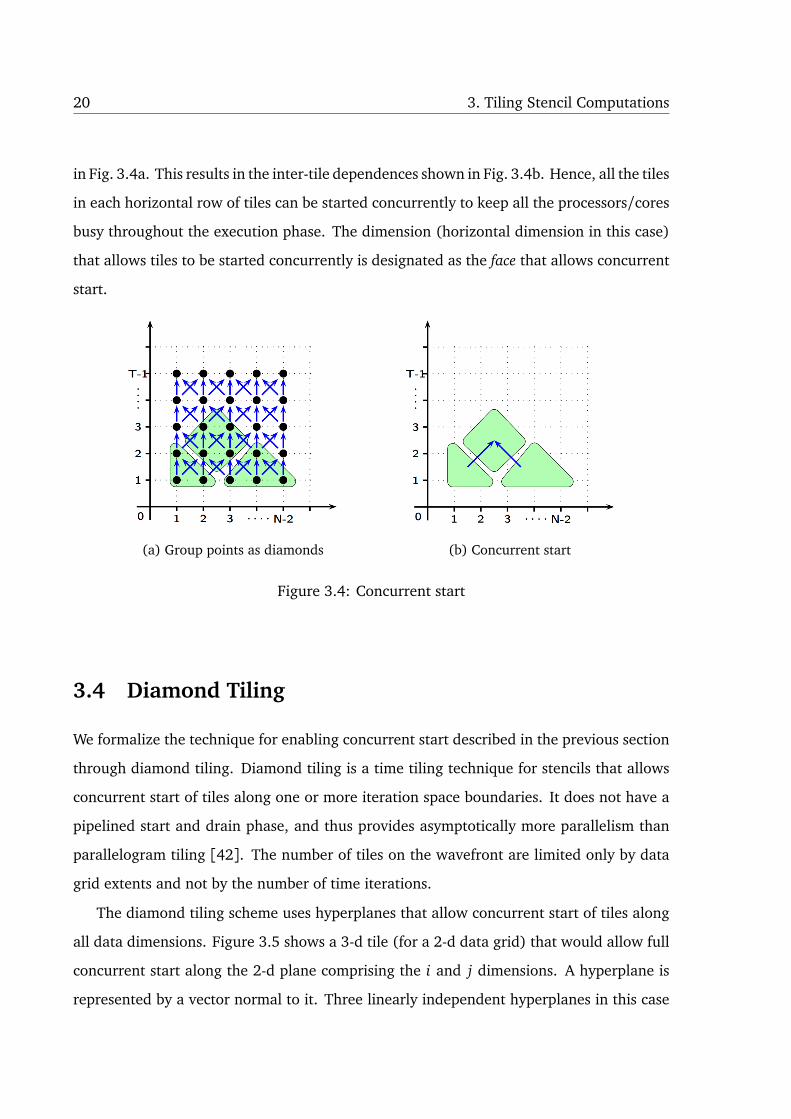
in Fig. 3.4a. This results in the inter-tile dependences shown in Fig. 3.4b. Hence, all the tiles

in each horizontal row of tiles can be started concurrently to keep all the processors/cores

busy throughout the execution phase. The dimension (horizontal dimension in this case)

that allows tiles to be started concurrently is designated as the face that allows concurrent

start.

(a) Group points as diamonds (b) Concurrent start

Figure 3.4: Concurrent start

3.4 Diamond Tiling

We formalize the technique for enabling concurrent start described in the previous section

through diamond tiling. Diamond tiling is a time tiling technique for stencils that allows

concurrent start of tiles along one or more iteration space boundaries. It does not have a

pipelined start and drain phase, and thus provides asymptotically more parallelism than

parallelogram tiling [42]. The number of tiles on the wavefront are limited only by data

grid extents and not by the number of time iterations.

The diamond tiling scheme uses hyperplanes that allow concurrent start of tiles along

all data dimensions. Figure 3.5 shows a 3-d tile (for a 2-d data grid) that would allow full

concurrent start along the 2-d plane comprising the i and j dimensions. A hyperplane is

represented by a vector normal to it. Three linearly independent hyperplanes in this case

3.4. Diamond Tiling 21

Figure 3.5: Tile shape for a 2-d LBM (d2q9 for example); arrows represent hyperplanes.

define a tile shape which is a hyper parallelepiped. The entire iteration space is uniformly

sliced into such hyper-parallelepipeds. The diamond tiling hyperplanes have the property

that the sum of the hyperplanes is a vector in the same direction as the time dimension –

this is also a direction along which there exists point-wise concurrent start in the iteration

space. In Figure 3.5, concurrent start is possible along both the space dimensions. This is

beneficial in cases where there are a large number of cores and they have to be efficiently

utilized. In particular, the i j plane in Figure 3.5 for example, allows point-wise concurrent

start. In practice, concurrent start along only a subset of space dimensions is sufficient to

keep all cores busy – we call this partial concurrent start. It results in simpler code while

providing the desired benefits.

This was a joint work with Vinayaka Bandishti [15, 43] and forms the basis for the

polyhedral optimizations for our LBM optimization framework.

Chapter 4

Our LBM Optimization Framework

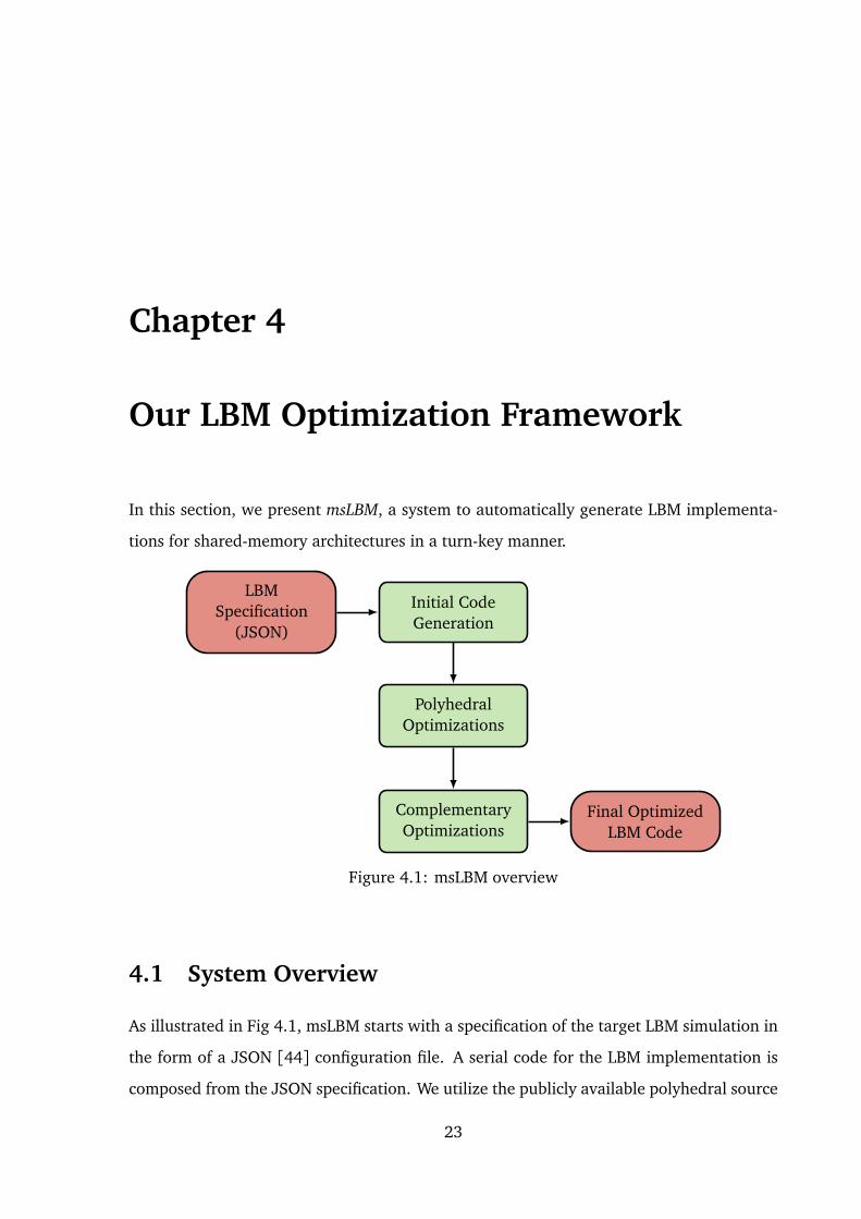
In this section, we present msLBM, a system to automatically generate LBM implementa-

tions for shared-memory architectures in a turn-key manner.

LBMSpecification

(JSON)

Initial CodeGeneration

PolyhedralOptimizations

ComplementaryOptimizations

Final OptimizedLBM Code

Figure 4.1: msLBM overview

4.1 System Overview

As illustrated in Fig 4.1, msLBM starts with a specification of the target LBM simulation in

the form of a JSON [44] configuration file. A serial code for the LBM implementation is

composed from the JSON specification. We utilize the publicly available polyhedral source

23

24 4. Our LBM Optimization Framework

to source optimizer, Pluto [45] for performing locality optimizations on the serial code.

Further complementary optimizations are implemented in Python with the generated serial

code as the input. The post-processed code is further tuned taking into consideration the

target architecture. The JSON notation provides an intuitive and compact way of capturing

the LBM simulation parameters. Parsing the configuration also becomes simpler.

4.2 Design Decisions

Unlike general implementations which employ two passes over the data grid per time step,

once for performing collision and a second time for advection, we chose to work with a

fused version of the LBM kernel. The data required for the collision at a domain node is

retrieved on demand from its neighbors and new PDFs at the current node are calculated

and updated. This results in better cache utilization and necessitates only a single pass

over the grid. Since we no longer have an explicit advection phase, a collision optimized

AoS data layout can be used.

Time tiling: Since the entire data grid has to be accessed once per time step, the band-

width requirement of LBM kernels is very high and they tend to be bottlenecked by the total

memory bandwidth available in the system. This situation worsens with the use of higher

order lattices (D3Q19, D3Q27, etc.). Time tiling is thus a very important optimization as

it improves temporal reuse and prevents computation from becoming memory bandwidth

bound by blocking along the time dimension.

LBM scheme: Although using a single grid to store data for the nodes in the domain

reduces the memory footprint of the implementation, it severely restricts time tiling as it

induces memory-based dependences. Fig. 4.2 illustrates this with a simple 1-d LBM case.

The collision phase for node k in time step t reads the required PDFs from the neighbors

in time step t − 1, computes new PDFs and updates the values in-place. Processing the

next node, k+ 1, for time step t, requires a value of node k from time step t − 1, and this

would be overwritten before its last use. Techniques like Compressed Grid work around this

4.2. Design Decisions 25

space

time

t = 0f1 f2 f3

k-1

t = 1f1 f2 f3

k-1

t = 2f1 f2 f3

k-1

t = 0f1 f2 f3

k

t = 1f1 f2 f3

k

t = 2f1 f2 f3

k

t = 0f1 f2 f3

k+1

t = 1f1 f2 f3

k+1

t = 2f1 f2 f3

k+1

1

Figure 4.2: Illustrative 1-d LBM with single grid

problem by specifying an order and direction for the processing and updates. However, this

creates complications when dealing with advanced boundary conditions [46] and hinders

further optimizations.

Our framework therefore adopts a two-grid, fused, pull scheme with an AoS data layout

for the LBM implementations.

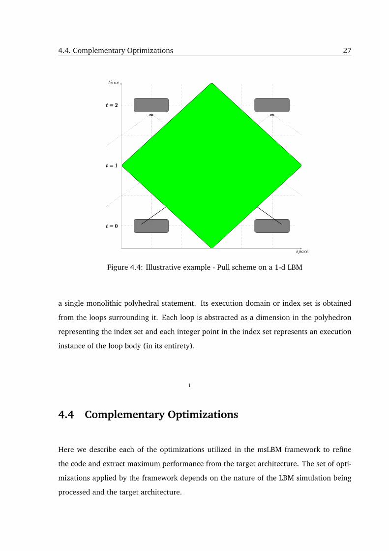
Enabling polyhedral transformations: With this configuration of LBM kernels, it is easy

to notice the similarity to normal stencils as illustrated in Fig. 4.4. The only difference is

that stencils store a single value at each node in the domain whereas LBM stores multiple

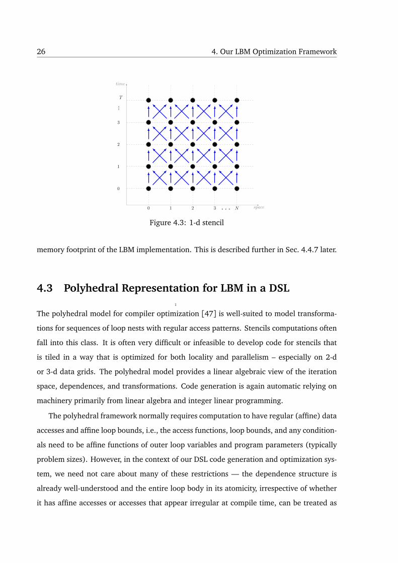
PDFs at each node depending on the lattice used. Notice that if all three points in the

rectangular box in Fig. 4.2 were collapsed to one point, the dependence structure becomes

identical to a 1-d stencil shown in Fig. 4.3. We exploit this inference to enable polyhedral

time tiling and subsequent optimizations on LBM implementations generated. By employ-

ing two grids, both the push and pull schemes become amenable to time tiling.

Per tile storage buffers could be used to perform storage compaction and reduce the

26 4. Our LBM Optimization Framework

space0 1 2 3 . . . N

time

0

1

2

3

...

T

1

Figure 4.3: 1-d stencil

memory footprint of the LBM implementation. This is described further in Sec. 4.4.7 later.

4.3 Polyhedral Representation for LBM in a DSL

The polyhedral model for compiler optimization [47] is well-suited to model transforma-

tions for sequences of loop nests with regular access patterns. Stencils computations often

fall into this class. It is often very difficult or infeasible to develop code for stencils that

is tiled in a way that is optimized for both locality and parallelism – especially on 2-d

or 3-d data grids. The polyhedral model provides a linear algebraic view of the iteration

space, dependences, and transformations. Code generation is again automatic relying on

machinery primarily from linear algebra and integer linear programming.

The polyhedral framework normally requires computation to have regular (affine) data

accesses and affine loop bounds, i.e., the access functions, loop bounds, and any condition-

als need to be affine functions of outer loop variables and program parameters (typically

problem sizes). However, in the context of our DSL code generation and optimization sys-

tem, we need not care about many of these restrictions — the dependence structure is

already well-understood and the entire loop body in its atomicity, irrespective of whether

it has affine accesses or accesses that appear irregular at compile time, can be treated as

4.4. Complementary Optimizations 27

space

time

t = 0f1 f2 f3

t = 1f1 f2 f3

t = 2f1 f2 f3

t = 0f1 f2 f3

t = 1f1 f2 f3

t = 2f1 f2 f3

t = 0f1 f2 f3

t = 1f1 f2 f3

t = 2f1 f2 f3

1

Figure 4.4: Illustrative example - Pull scheme on a 1-d LBM

a single monolithic polyhedral statement. Its execution domain or index set is obtained

from the loops surrounding it. Each loop is abstracted as a dimension in the polyhedron

representing the index set and each integer point in the index set represents an execution

instance of the loop body (in its entirety).

4.4 Complementary Optimizations

Here we describe each of the optimizations utilized in the msLBM framework to refine

the code and extract maximum performance from the target architecture. The set of opti-

mizations applied by the framework depends on the nature of the LBM simulation being

processed and the target architecture.

28 4. Our LBM Optimization Framework

4.4.1 Simplification of the LBM Kernel

We use SymPy [48], a Python library for symbolic mathematics to simplify the LBM kernel.

SymPy enables us to do common sub-expression elimination (CSE) across multiple state-

ments, thereby reducing the number of floating point operations (FP-ops) required for the

LBM kernel. In some cases, we observed that the compiler might not be able to achieve

this even with a relaxed floating point model.

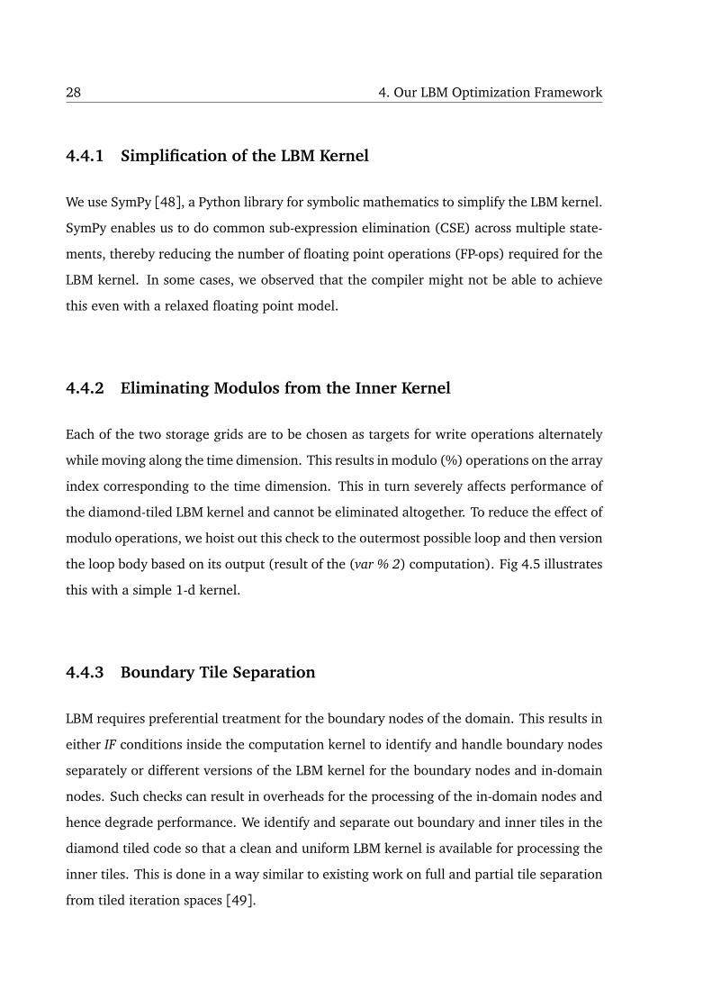
4.4.2 Eliminating Modulos from the Inner Kernel

Each of the two storage grids are to be chosen as targets for write operations alternately

while moving along the time dimension. This results in modulo (%) operations on the array

index corresponding to the time dimension. This in turn severely affects performance of

the diamond-tiled LBM kernel and cannot be eliminated altogether. To reduce the effect of

modulo operations, we hoist out this check to the outermost possible loop and then version

the loop body based on its output (result of the (var % 2) computation). Fig 4.5 illustrates

this with a simple 1-d kernel.

4.4.3 Boundary Tile Separation

LBM requires preferential treatment for the boundary nodes of the domain. This results in

either IF conditions inside the computation kernel to identify and handle boundary nodes

separately or different versions of the LBM kernel for the boundary nodes and in-domain

nodes. Such checks can result in overheads for the processing of the in-domain nodes and

hence degrade performance. We identify and separate out boundary and inner tiles in the

diamond tiled code so that a clean and uniform LBM kernel is available for processing the

inner tiles. This is done in a way similar to existing work on full and partial tile separation

from tiled iteration spaces [49].

4.4. Complementary Optimizations 29

for (t = 0; t < nT; t++)

for (x = 1; x < nX; x++)

A[(t+1)%2][x] =

(1/3)*(A[t%2][x-1] + A[t%2][x]

+ A[t%2][x+1]);

(a) Loop nest with modulo

for (t = 0; t < nT; t++)

if(t % 2 == 0)

for (x = 1; x < nX; x++)

A[1][x] =

(1/3)*(A[0][x-1] + A[0][x] +

A[0][x+1]);

else

for (x = 1; x < nX; x++)

A[0][x] =

(1/3)*(A[1][x-1] + A[1][x] +

A[1][x+1]);

(b) Loop nest with modulo hoisted

Figure 4.5: Modulo hoisting example

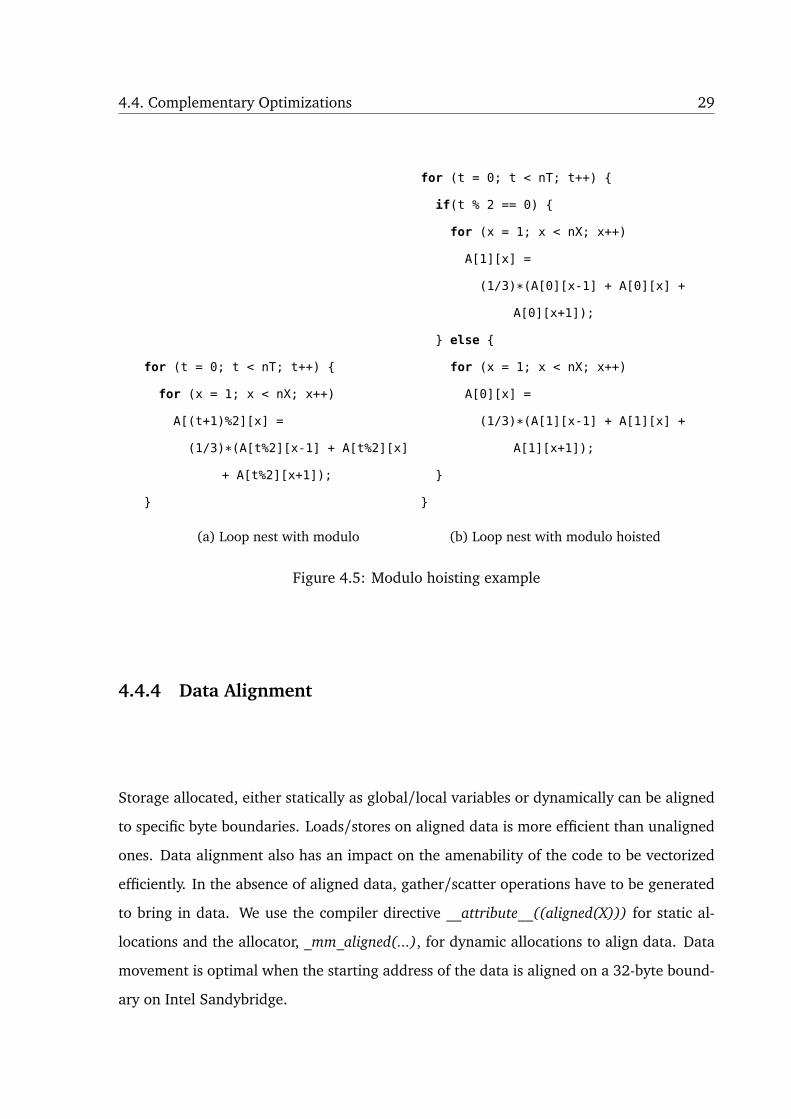
4.4.4 Data Alignment

Storage allocated, either statically as global/local variables or dynamically can be aligned

to specific byte boundaries. Loads/stores on aligned data is more efficient than unaligned

ones. Data alignment also has an impact on the amenability of the code to be vectorized

efficiently. In the absence of aligned data, gather/scatter operations have to be generated

to bring in data. We use the compiler directive __attribute__((aligned(X))) for static al-

locations and the allocator, _mm_aligned(...), for dynamic allocations to align data. Data

movement is optimal when the starting address of the data is aligned on a 32-byte bound-

ary on Intel Sandybridge.

30 4. Our LBM Optimization Framework

4.4.5 Inlining & Unrolling

For most part of the transformations, we treat the LBM kernel as a black box. But this

might prohibit the compiler from performing certain optimizations. Inlining the LBM ker-

nel eliminates overheads associated with function invocations. Unrolling by a suitable

factor provides the compiler opportunities to efficiently schedule instructions to achieve a

high sustained compute performance. Combined with boundary tile separation, the LBM

kernel for the inner tiles can be both inlined and unrolled. We rely on the native compiler’s

(icc) automatic vectorization to perform the rest.

4.4.6 Predicated SIMDization

for(..;..;..)

if(v5<v6)

v1 += v3;

(a) Loop nest with an IF conditional

for(..;..;..)

vcmppi_lt k7 , v5, v6

vaddpi v1k7, v1, v3

(b) Predicated SIMD code for loop body

Figure 4.6: Predicated SIMD example

In the presence of obstacles in the domain, which can be represented either using a

flag for each node or an analytic expression that is evaluated at each node, vectorizing the

code becomes difficult. Predicated SIMD instructions, which allow per lane conditional

flow, can help vectorize such cases. A simple example is shown in Fig 4.6. We structure

our code in a way that makes it easy for the compiler to generate predicated SIMD code.

4.4.7 Memory Optimization

Recall that we chose to use a two grid model since the resulting data dependences allowed

application of time tiling transformations. Domain scientists are often interested in weak

4.4. Complementary Optimizations 31

scaling for LBM. Using a two-grid approach thus allows them to only run half the data set

they could have, given an upper limit on the available main memory. It is however possible

to reduce the memory footprint of the two grid optimized code post-transformation to the

single grid one on a per tile basis, i.e., for sequential execution of a single tile on a core.

This is achieved with a modulo mapping which emulates a rotating buffer. Consider a 1-d

LBM with N data points in all with time loop t and space loop i – this would consume

2 ∗ N lattice elements of storage with two grids and N with a single grid. If a grid or a

portion of the grid (a tile) is executed sequentially, note that the write at location (t, i)

can reuse the location of iteration (t − 1, i − 1) since the last read for data generated at

(t − 1, i − 1) has already happened at (t, i). Hence, only a rotating buffer of size N + 1

lattice elements is needed as opposed to 2 ∗N . Analogously, for 2-d LBMs, the storage can

be reduced from 2∗N 2 elements to N 2+N +1 elements, and for a 3-d stencil, from 2∗N 3

elements to N 3 + N 2 + N + 1. Hence, using a two grid approach and then reducing the

storage requirement is a cleaner way for automatic optimization purposes. Techniques for

analyzing and achieving such mappings exist [50, 51, 52].

4.4.8 Tile Sizes

Although the determination of the right tile sizes, both for locality and parallelism, is critical

for single thread performance and scaling, this is a straightforward problem in a domain-

specific context where the computation and the transformation on it is known and com-

pletely understood. Due to lack of space, we do not discuss this issue further or present a

model for selection of tile sizes.

Chapter 5

Experimental Evaluation

In this chapter, we evaluate our code generator by presenting results on a range of LBM

simulations and benchmarks.

5.1 Experimental Setup

We empirically evaluate performance on an Intel Xeon based on the Sandybridge microar-

chitecture. Its architectural details are presented in Table 5.1. The machine is a dual-socket

system with each socket seating a Xeon E5 2680 processor with a total of 64 GB of non-

ECC RAM. Code generated by our framework is labeled Our (mslbm). mslbm-no-vec is

code we generate but without the post processing transformations that we perform to en-

able vectorization. The difference between the two thus captures the efficiency and benefit

of vectorization. The Intel Sandybridge includes the 256-bit Advanced Vector Extensions

(AVX). All computations used herein employ double-precision floating point arithmetic.

5.2 Benchmarks

For evaluation purposes, we choose a set of benchmarks that represents a wide diversity of

LBM computations in terms of dimensionality, arithmetic to memory operation ratios, par-

ticipating neighbors, and boundary conditions. Each of the benchmarks used is described

33

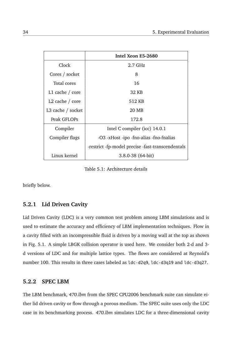
34 5. Experimental Evaluation

Intel Xeon E5-2680

Clock 2.7 GHz

Cores / socket 8

Total cores 16

L1 cache / core 32 KB

L2 cache / core 512 KB

L3 cache / socket 20 MB

Peak GFLOPs 172.8

Compiler Intel C compiler (icc) 14.0.1

Compiler flags -O3 -xHost -ipo -fno-alias -fno-fnalias

-restrict -fp-model precise -fast-transcendentals

Linux kernel 3.8.0-38 (64-bit)

Table 5.1: Architecture details

briefly below.

5.2.1 Lid Driven Cavity

Lid Driven Cavity (LDC) is a very common test problem among LBM simulations and is

used to estimate the accuracy and efficiency of LBM implementation techniques. Flow in

a cavity filled with an incompressible fluid is driven by a moving wall at the top as shown

in Fig. 5.1. A simple LBGK collision operator is used here. We consider both 2-d and 3-

d versions of LDC and for multiple lattice types. The flows are considered at Reynold’s

number 100. This results in three cases labeled as ldc-d2q9, ldc-d3q19 and ldc-d3q27.

5.2.2 SPEC LBM

The LBM benchmark, 470.lbm from the SPEC CPU2006 benchmark suite can simulate ei-

ther lid driven cavity or flow through a porous medium. The SPEC suite uses only the LDC

case in its benchmarking process. 470.lbm simulates LDC for a three-dimensional cavity

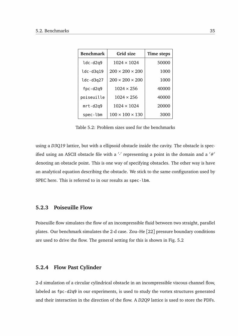
5.2. Benchmarks 35

Benchmark Grid size Time steps

ldc-d2q9 1024× 1024 50000

ldc-d3q19 200× 200× 200 1000

ldc-d3q27 200× 200× 200 1000

fpc-d2q9 1024× 256 40000

poiseuille 1024× 256 40000

mrt-d2q9 1024× 1024 20000

spec-lbm 100× 100× 130 3000

Table 5.2: Problem sizes used for the benchmarks

using a D3Q19 lattice, but with a ellipsoid obstacle inside the cavity. The obstacle is spec-

ified using an ASCII obstacle file with a ′·′ representing a point in the domain and a ′#′

denoting an obstacle point. This is one way of specifying obstacles. The other way is have

an analytical equation describing the obstacle. We stick to the same configuration used by

SPEC here. This is referred to in our results as spec-lbm.

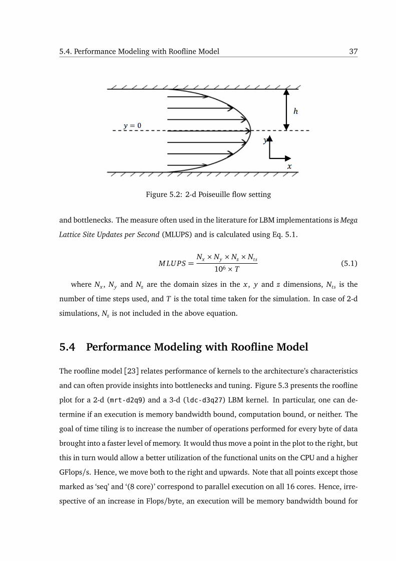
5.2.3 Poiseuille Flow

Poiseuille flow simulates the flow of an incompressible fluid between two straight, parallel

plates. Our benchmark simulates the 2-d case. Zou–He [22] pressure boundary conditions

are used to drive the flow. The general setting for this is shown in Fig. 5.2

5.2.4 Flow Past Cylinder

2-d simulation of a circular cylindrical obstacle in an incompressible viscous channel flow,

labeled as fpc-d2q9 in our experiments, is used to study the vortex structures generated

and their interaction in the direction of the flow. A D2Q9 lattice is used to store the PDFs.

36 5. Experimental Evaluation

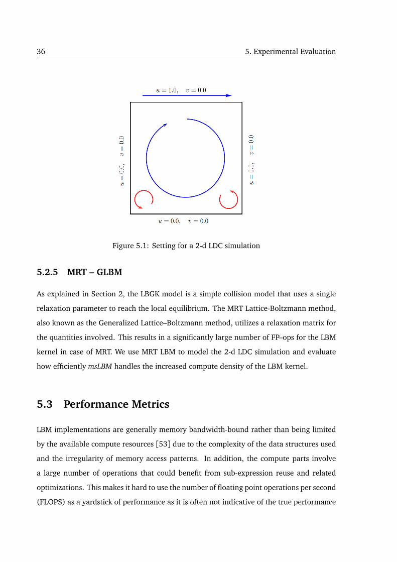
Figure 5.1: Setting for a 2-d LDC simulation

5.2.5 MRT – GLBM

As explained in Section 2, the LBGK model is a simple collision model that uses a single

relaxation parameter to reach the local equilibrium. The MRT Lattice-Boltzmann method,

also known as the Generalized Lattice–Boltzmann method, utilizes a relaxation matrix for

the quantities involved. This results in a significantly large number of FP–ops for the LBM

kernel in case of MRT. We use MRT LBM to model the 2-d LDC simulation and evaluate

how efficiently msLBM handles the increased compute density of the LBM kernel.

5.3 Performance Metrics

LBM implementations are generally memory bandwidth-bound rather than being limited

by the available compute resources [53] due to the complexity of the data structures used

and the irregularity of memory access patterns. In addition, the compute parts involve

a large number of operations that could benefit from sub-expression reuse and related

optimizations. This makes it hard to use the number of floating point operations per second

(FLOPS) as a yardstick of performance as it is often not indicative of the true performance

5.4. Performance Modeling with Roofline Model 37

Figure 5.2: 2-d Poiseuille flow setting

and bottlenecks. The measure often used in the literature for LBM implementations is Mega

Lattice Site Updates per Second (MLUPS) and is calculated using Eq. 5.1.

M LU PS =Nx × Ny × Nz × Nts

106 × T(5.1)

where Nx , Ny and Nz are the domain sizes in the x , y and z dimensions, Nts is the

number of time steps used, and T is the total time taken for the simulation. In case of 2-d

simulations, Nz is not included in the above equation.

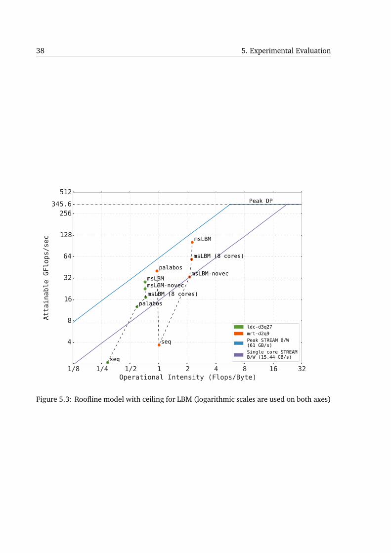
5.4 Performance Modeling with Roofline Model

The roofline model [23] relates performance of kernels to the architecture’s characteristics

and can often provide insights into bottlenecks and tuning. Figure 5.3 presents the roofline

plot for a 2-d (mrt-d2q9) and a 3-d (ldc-d3q27) LBM kernel. In particular, one can de-

termine if an execution is memory bandwidth bound, computation bound, or neither. The

goal of time tiling is to increase the number of operations performed for every byte of data

brought into a faster level of memory. It would thus move a point in the plot to the right, but

this in turn would allow a better utilization of the functional units on the CPU and a higher

GFlops/s. Hence, we move both to the right and upwards. Note that all points except those

marked as ‘seq’ and ‘(8 core)’ correspond to parallel execution on all 16 cores. Hence, irre-

spective of an increase in Flops/byte, an execution will be memory bandwidth bound for

38 5. Experimental Evaluation

1/8 1/4 1/2 1 2 4 8 16 32Operational Intensity (Flops/Byte)

4

8

16

32

64

128

256345.6

512

Atta

inab

le G

Flop

s/se

c

palabos

seq

msLBM-novec

msLBM (8 cores)

msLBM

seq

palabosmsLBM (8 cores)msLBM-novecmsLBM

Peak DP

ldc-d3q27mrt-d2q9Peak STREAM B/W(61 GB/s)Single core STREAMB/W (15.44 GB/s)

Figure 5.3: Roofline model with ceiling for LBM (logarithmic scales are used on both axes)

5.5. Performance Analysis 39

a sufficiently large number of cores. For mrt-d2q9, Palabos provides performance close to

the ceiling possible for an operational intensity of 1.0. Our framework improves the op-

erational intensity of the kernel to 2.26 flops/byte and is able to obtain performance very

close to the maximum possible for that particular operational intensity. With ldc-d3q27,

Palabos improves the operational intensity, but msLBM obtains further improvement over

that in both operational intensity and peak achievable performance.

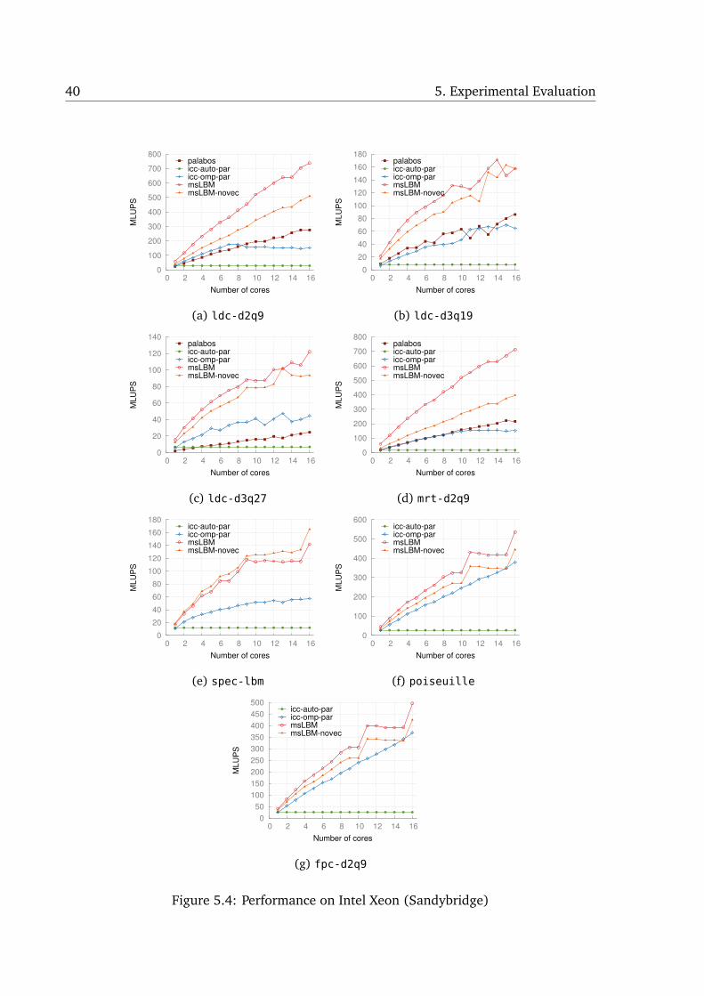
5.5 Performance Analysis

Fig. 5.4 presents results for all benchmarks reporting MLUPS on the y-axis. We observe

that msLBM provides significantly better single thread performance due to better locality

optimization and allows good or better scaling than Palabos. For spec-lbm, poiseuille,

fpc-d2q9 (Fig. 5.4e, 5.4f, 5.4g), we were unable to find a way to express them with Palabos

– hence no results with Palabos are presented in those cases.

As is evident from the graphs, the results we see for icc-auto-par on multiple cores

is just its sequential performance. We observed that icc was unable to parallelize the core

loop nest due to conservatively assumed dependences likely arising from imprecise alias in-

formation. We thus manually parallelized the code in a straightforward way using OpenMP

and this is reported in the graphs as (icc-omp-par). The outermost space loop was marked

parallel. The lower single thread performance for icc-omp-par and poorer scaling con-

firms earlier remarks that the original execution order was memory bandwidth-bound. The

difference between mslbm-no-vec and mslbm quantifies the improvement achieved with

vectorization. We consistently observe a lower vectorization efficiency for the 3-d cases

that in the 2-d ones. Note that the trip counts for the loops in the 3-d case are significantly

lower leading to a larger fraction of partial tiles. Improving vectorization efficiency for the

3-d cases is one of the subjects of our future work.

In most cases, we observe ideal or close to ideal scaling with mslbm. The spec-lbm

data grid as mentioned earlier involves an obstacle which is of size comparable to the data

grid itself. Our code generator currently only supports extraction of a single degree of

40 5. Experimental Evaluation

0

100

200

300

400

500

600

700

800

0 2 4 6 8 10 12 14 16

MLU

PS

Number of cores

palabosicc-auto-paricc-omp-parmsLBMmsLBM-novec

(a) ldc-d2q9

0

20

40

60

80

100

120

140

160

180

0 2 4 6 8 10 12 14 16

MLU

PS

Number of cores

palabosicc-auto-paricc-omp-parmsLBMmsLBM-novec

(b) ldc-d3q19

0

20

40

60

80

100

120

140

0 2 4 6 8 10 12 14 16

MLU

PS

Number of cores

palabosicc-auto-paricc-omp-parmsLBMmsLBM-novec

(c) ldc-d3q27

0

100

200

300

400

500

600

700

800

0 2 4 6 8 10 12 14 16

MLU

PS

Number of cores

palabosicc-auto-paricc-omp-parmsLBMmsLBM-novec

(d) mrt-d2q9

0

20

40

60

80

100

120

140

160

180

0 2 4 6 8 10 12 14 16

MLU

PS

Number of cores

icc-auto-paricc-omp-parmsLBMmsLBM-novec

(e) spec-lbm

0

100

200

300

400

500

600

0 2 4 6 8 10 12 14 16

MLU

PS

Number of cores

icc-auto-paricc-omp-parmsLBMmsLBM-novec

(f) poiseuille

0

50

100

150

200

250

300

350

400

450

500

0 2 4 6 8 10 12 14 16

MLU

PS

Number of cores

icc-auto-paricc-omp-parmsLBMmsLBM-novec

(g) fpc-d2q9

Figure 5.4: Performance on Intel Xeon (Sandybridge)

5.5. Performance Analysis 41

parallelism, and as a result we run out of useful work here. This is purely a limitation of

the current state of implementation and the scaling is expected to be better when multiple

degrees of parallelism are extracted in such cases. The anomalies in performance and

scaling for msLBM in some cases, when close to the maximum number of cores, is due to: (1)

the number of tiles not being perfectly divisible by the number of cores, and (2) difficulty

in reproducing performance for the maximum number of cores due to interference from

certain internal OS kernel processes.

0

1000

2000

3000

4000

5000

6000

7000

0 2 4 6 8 10 12 14 16

ME

UP

S

Number of cores

ldc-d2q9ldc-d3q19ldc-d3q27mrt-d2q9spec-lbmfpc-d2q9poiseuille

Figure 5.5: Comparison of MEUPS across benchmarks for mslbm

Figure 5.5 shows the performance of mslbm generated code for different benchmarks in

a single graph in a way that allows comparison of the performance achieved with different

models. Using MLUPS for the comparison of different LBM implementations having distinct

lattice arrangements is not considered fair. To this end, Million Elementary Updates Per

42 5. Experimental Evaluation

Second (MEUPS), as proposed in [30], is obtained by multiplying the MLUPS value with

n−1, where n is the number of PDFs present in the lattice used. The y-axis in MEUPS thus

makes the comparison meaningful across different configurations.

In case of LDC benchmarks, the accuracy of the solution was verified by comparing the

center-line velocities to the results reported by Ghia et al. [54]. For Poiseuille flows, since

the analytical solution is available, we verified the parabolic velocity profile of our steady

state flow.

We also comment on how our code performs when compared with the results obtained

by Nguyen et al. [5] with the 3.5d tiling and other optimizations they had performed by

hand. Their implementation is not publicly available for a direct comparison, and the

performance reported therein was in MLUPS for SPEC LBM on a 4-core Nehalem core i7

machine running at 3.2 GHz. Since it would not be meaningful or fair to compare perfor-

mance on our Intel Sandybridge against an older microarchitecture, we executed our code

on 4 cores of a 2.6 GHz Westmere Xeon processor that shares the same microarchitecture as

theirs – we obtained a performance of 40 MLUPS. Normalizing the 80 MLUPS performance

of [5] to 2.6 GHz yields 67.5 MLUPS. We have thus achieved 60% of the performance of

a heavily hand-tuned code. We believe that the gap is primarily due to the efficiency of

vectorization and SPEC LBM is particularly a challenging case.

In summary, msLBM achieves a mean (geometric) speedup of 3× over Palabos, and a

mean (geometric) speedup of 2.6× over a native production compiler (icc-omp-par) while

running on 16 cores. In addition, we obtain a speedup of 2.47× over the native production

on SPEC LBM. Our primary objectives have been to improve over the state-of-the-art with

respect to performance while improving programmer productivity, and to present LBM

as a class to demonstrate domain-specific compilation and optimization. A more detailed

modeling of the compute peak and the memory bandwidth peak is out of this work’s scope.

An analysis of how far we are away from the absolute peak and how much of that gap could

be bridged is left for future work. We plan to employ a model such as the roofline model

to study this aspect.

Chapter 6

Related Work

Quite a lot of work has gone into optimizing stencil computations. They can be broadly

divided into two – compiler optimizations [55, 56, 57, 12] and domain specific optimization

techniques [58, 59, 60, 61, 62, 63, 64, 36]. LLVM Polly [65], R-Stream [66], and IBM

XL [67] are some of the production compilers that include polyhedral framework based

stencil optimization techniques. Among the domain specific works, Pochoir [36] stands out.

Being able to infer more information about the domain, it is able to provide much higher

performance when compared to the general transformation frameworks in the production

compilers.

Pochoir [36] is a highly tuned stencil specific compiler and runtime system for multi-

cores. It provides a C++ template library using which a programmer can describe a speci-

fication of a stencil in terms of dimensions, width of the stencil, its shape etc.. Pochoir uses

a cache-oblivious tiling mechanism and a work stealing scheduler to provide load balanced

execution. We outperform Pochoir with the diamond tiling scheme by as much as 2× in

some cases. Strzodka et al. [61] present a technique, cache accurate time skewing (CATS),

for tiling stencils. They claim that tiling in only some dimensions is more beneficial than

tiling all the available dimensions in 3-d cases. The same result is achieved though our

lower dimensional concurrent start technique. Henretty et al. [13] present a data layout

transformation technique to improve vectorization. Since the performance of aligned and

43

44 6. Related Work

unaligned loads on modern architectures is comparable, we did not explore layout trans-

formations for vectorization, but instead relied on Intel compiler’s auto-vectorization after

automatic application of enabling transformations within a tile. This was enough to extract

good SIMD performance from these codes. Krishnamoorthy et al. [57] addressed concur-

rent start when tiling stencil computations. However, the approach worked by starting with

a valid tiling and correcting it to allow concurrent start. This was done via overlapped ex-

ecution of tiles (overlapped tiling) or by splitting a tile into sub-tiles (split tiling).

Figure 6.1: Compressed Grid technique [2]

Several past works [68, 69, 70] have focused on optimizing LBM computations for both

shared memory and distributed memory architectures.

Time blocking is an optimization that can greatly improve performance of LBM com-

putations. The earliest work to look at time blocking for LBM was Wilke et al. [2]. They

manually perform both 1-d blocking and 2-d blocking on the LBM code with a Compressed

Grid (Fig. 6.1). Compressed Grid technique reduces the storage required from two data

grids to one grid and a constant extra space. Iteration order is reversed after each time

step. The data dependencies are lifted by storing the result of each cell update in a shifted

position and enlarging the lattice by one layer of cells in each dimension.

1-d blocking was not found to provide any performance benefits. Fig. 6.2 illustrates 2-d

blocking of a lattice with a 4x4 blocking factor. With 2-d blocking using a blocking factor

of 16x16, they were able to improve the performance. But this imposes an order on the

processing of tiles; diagonally down, towards the left. This severely cripples the available

parallelism. They conclude that manually generating cache optimized time tiled codes for

45

Figure 6.2: 2-d blocking (4x4 blocking factor) by Wilke et al. [2]

LBM is tedious and error prone.

Nitsure et al. [3, 4] proposed a cache oblivious algorithm for LBM, COLBA. It uses

virtual domain decomposition to generate tasks and parallelization is done using Intel’s

Workqueuing Model [71] for OpenMP. The algorithm is recursive and utilizes a time block-

ing factor (TB) when generating tasks. They report that they had found it difficult to work

with the usual OpenMP parallel and parallel for pragmas due to the recursive nature of

the algorithm and also resulted in ‘orphan’ directives that never spawned threads. The

execution is pipelined and suffers from pipeline fill and drain phases.

Fig. 6.3 shows the domain being decomposed and represented as a tree. The nodes

of the tree constitute the tasks for the Intel Taskq model. Tasks 2 and 3 have to wait for

the completion of task 1 to start. This clearly illustrates the pipeline fill and drain phases

in the execution of the program. Since the recursive domain decomposition generates a

queue of tasks to be processed before the threads start executing them in parallel, a locking

mechanism has to be present to prevent the execution of tasks whose dependences have

not yet been fulfilled. To this end, they use a 1-d array of omp lock t variables called the

synchronization table with one lock entry per domain. Before solving its own domain, each

thread checks whether the left and bottom domains are unlocked. If both neighbors have

already been unlocked, then it will first solve and then unlock its own domain, otherwise

46 6. Related Work

it will wait, until both neighbors have been solved.

Figure 6.3: COLBA - The mapping of virtually decomposed domains to a tree [3, 4]

(a) Overlapped computation

(b) Sequential section in the prologue of

each XY-block

Figure 6.4: 3.5d blocking [5]

The 3.5d Blocking technique by Nguyen et al. [5] is a recent effort towards time-tiling

LBM computations. Instead of tiling all the three space dimensions, they tile two of the

outermost space dimensions and execute the third dimension in each tile as a whole. They

call this scheme 2.5d blocking. This along with tiling of the time dimension results in 3.5d

47

blocking scheme. Fig. 6.4a shows their 2.5d blocking of the 3-d space. dim2.5DX and dim2.5D

Y

represent the tile sizes along the two outermost space dimensions. The steps S1 . . . S13

(Fig. 6.4b) are performed in chronological order. The parallel 3.5d blocking algorithm thus

involves some amount of overlapped computation and a sequential section in the prologue

of each XY-block processed by a thread.

A comprehensive framework that can address some of the shortcomings of previous

works and automatically generate code that achieves high performance on different archi-

tectures has been missing and our work is a step in that direction.

Chapter 7

Conclusions

We proposed an optimizing code generator for a class of LBM computations with the objec-

tive to achieve high performance with no user effort involved beyond providing a high-level

specification of the problem. Few studies in the past had looked at time tiling for LBM codes

and had done so manually. We exploited an important similarity between typical represen-

tative stencil kernels and LBM to enable polyhedral loop transformations and in turn time

tiling for LBM. Besides polyhedral transformations, we also describe a number of other

complementary transformations and post processing necessary to obtain good parallel and

SIMD performance.

Experimental results for standard LBM simulations like Lid-Driven Cavity, Flow Past

Cylinder, and Poiseuille Flow showed that our scheme consistently outperformed Palabos

— on average by 3× while running on 16 cores of an Intel Xeon Sandybridge system. Our

system shows a mean (geometric) speedup of 2.6× over native production compiler when

running on 16 cores. We also obtain a very significant improvement of 2.47× over the

native production compiler on the SPEC LBM benchmark.

We also characterized the performance of LBM with the Roofline performance model

and concluded that msLBM obtains further improvement over Palabos in both operational

intensity and peak achievable performance.

Exploring a two dimensional task distribution using dynamic scheduling, especially for

3-d simulations, to improve the overall scalability is another thing that has to be tried.

49

Bibliography

[1] “Xflow.” [Online]. Available at: http://www.accsimia-software.com/wp-content/

uploads/2013/07/XFlow_productsheet-July-2013.pdf

[2] J. Wilke, T. Pohl, M. Kowarschik, and U. Rüde, “Cache performance optimizations

for parallel lattice boltzmann codes,” in Euro-Par 2003 Parallel Processing. Springer,

2003, pp. 441–450.

[3] A. Nitsure, K. Iglberger, U. Rüde, C. Feichtinger, G. Wellein, and G. Hager, “Opti-

mization of cache oblivious lattice boltzmann method in 2d and 3d,” in Frontiers in

Simulation: Simulationstechnique–19th Symposium in Hannover, 2006, pp. 265–270.

[4] S. Donath, K. Iglberger, G. Wellein, T. Zeiser, A. Nitsure, and U. Rude, “Performance

comparison of different parallel lattice boltzmann implementations on multi-core

multi-socket systems,” International Journal of Computational Science and Engineer-

ing, vol. 4, no. 1, pp. 3–11, 2008.

[5] A. D. Nguyen, N. Satish, J. Chhugani, C. Kim, and P. Dubey, “3.5-d blocking optimiza-

tion for stencil computations on modern cpus and gpus.” in Supercomputing (SC),

2010, pp. 1–13.

[6] S. Succi, The lattice Boltzmann equation: for fluid dynamics and beyond. Oxford

university press, 2001.

[7] B. Chopard, M. B. Begacem, A. Parmigiani, and J. Latt, “A lattice boltzmann

simulation of the rhone river,” International Journal of Modern Physics C, p. 1340008,

2013. [Online]. Available at: http://dx.doi.org/10.1142/S0129183113400081

51

52 BIBLIOGRAPHY

[8] N. Satish, C. Kim, J. Chhugani, H. Saito, R. Krishnaiyer, M. Smelyanskiy, M. Girkar,

and P. Dubey, “Can traditional programming bridge the ninja performance gap for

parallel computing applications?” in Proceedings of the 39th Annual International

Symposium on Computer Architecture, 2012, pp. 440–451.

[9] Y. Song and Z. Li, “New tiling techniques to improve cache temporal locality,” in ACM

SIGPLAN PLDI, 1999, pp. 215–228.

[10] D. Wonnacott, “Achieving scalable locality with time skewing,” International Journal

of Parallel Programming, vol. 30, no. 3, pp. 1–221, 2002.

[11] S. Krishnamoorthy, M. Baskaran, U. Bondhugula, J. Ramanujam, A. Rountev, and

P. Sadayappan, “Effective automatic parallelization of stencil computations,” in ACM

Sigplan Notices, vol. 42, no. 6. ACM, 2007, pp. 235–244.

[12] U. Bondhugula, A. Hartono, J. Ramanujam, and P. Sadayappan, “A practical automatic

polyhedral program optimization system,” in ACM SIGPLAN Conference on Program-

ming Language Design and Implementation (PLDI), Jun. 2008.

[13] T. Henretty, K. Stock, L.-N. Pouchet, F. Franchetti, J. Ramanujam, and P. Sadayappan,

“Data layout transformation for stencil computations on short simd architectures,”

in ETAPS International Conference on Compiler Construction (CC’11), Mar. 2011, pp.

225–245.

[14] J. Holewinski, L.-N. Pouchet, and P. Sadayappan, “High-performance code generation

for stencil computations on GPU architectures,” in ICS, 2012, pp. 311–320.

[15] V. Bandishti, I. Pananilath, and U. Bondhugula, “Tiling stencil computations to maxi-

mize parallelism,” in Supercomputing (SC), 2012, pp. 40:1–40:11.

[16] T. Henretty, R. Veras, F. Franchetti, L.-N. Pouchet, J. Ramanujam, and P. Sadayappan,

“A stencil compiler for short-vector simd architectures,” in ACM ICS, 2013.

[17] T. Grosser, A. Cohen, J. Holewinski, P. Sadayappan, and S. Verdoolaege, “Hybrid

hexagonal/classical tiling for gpus,” in CGO, 2014, p. 66.

BIBLIOGRAPHY 53

[18] T. Pohl, M. Kowarschik, J. Wilke, K. Iglberger, and U. Rüde, “Optimization and profil-

ing of the cache performance of parallel lattice boltzmann codes,” Parallel Processing

Letters, vol. 13, no. 04, pp. 549–560, 2003.

[19] “Palabos.” [Online]. Available at: http://www.palabos.org/

[20] S. Hou, Q. Zou, S. Chen, G. Doolen, and A. C. Cogley, “Simulation of cavity flow by

the lattice boltzmann method,” J. Comput. Phys., vol. 118, no. 2, pp. 329–347, May

1995. [Online]. Available at: http://dx.doi.org/10.1006/jcph.1995.1103

[21] D. d’Humières, P. Lallemand, L.-S. Luo et al., “Lattice boltzmann equation on a two-

dimensional rectangular grid,” Journal of Computational Physics, vol. 172, no. 2, pp.

704–717, 2001.

[22] Q. Zou and X. He, “On pressure and velocity boundary conditions for the lattice Boltz-

mann BGK model,” Physics of Fluids (1994-present), vol. 9, no. 6, pp. 1591–1598,

1997.

[23] G. Ofenbeck, R. Steinmann, V. Caparros, D. G. Spampinato, and M. Püschel, “Apply-

ing the roofline model,” in IEEE International Symposium on Performance Analysis of

Systems and Software (ISPASS), 2014.

[24] S. Chen and G. D. Doolen, “Lattice boltzmann method for fluid flows,” Annual review

of fluid mechanics, vol. 30, no. 1, pp. 329–364, 1998.

[25] P. L. Bhatnagar, E. P. Gross, and M. Krook, “A model for collision processes in gases.

i. small amplitude processes in charged and neutral one-component systems,” Phys.

Rev., vol. 94, pp. 511–525, May 1954.

[26] D. d’Humières, “Multiple–relaxation–time lattice boltzmann models in three dimen-

sions,” Philosophical Transactions of the Royal Society of London. Series A: Mathemati-

cal, Physical and Engineering Sciences, vol. 360, no. 1792, pp. 437–451, 2002.

[27] Q. Zou and X. He, “On pressure and velocity flow boundary conditions and bounce-

back for the lattice boltzmann bgk model,” arXiv preprint comp-gas/9611001, 1996.

54 BIBLIOGRAPHY

[28] K. Mattila, J. Hyväluoma, T. Rossi, M. Aspnäs, and J. Westerholm, “An efficient swap

algorithm for the lattice boltzmann method,” Computer Physics Communications, vol.

176, no. 3, pp. 200–210, 2007.

[29] M. Wittmann, T. Zeiser, G. Hager, and G. Wellein, “Comparison of different propa-

gation steps for lattice boltzmann methods,” Computers & Mathematics with Applica-

tions, vol. 65, no. 6, pp. 924–935, 2013.

[30] A. G. Shet, S. H. Sorathiya, S. Krithivasan, A. M. Deshpande, B. Kaul, S. D. Sherlekar,

and S. Ansumali, “Data structure and movement for lattice-based simulations,” Phys.

Rev. E, vol. 88, p. 013314, Jul 2013.

[31] P. Feautrier, “Automatic parallelization in the polytope model,” in The Data Parallel

Programming Model. Springer, 1996, pp. 79–103.

[32] A. Lim and M. S. Lam, “Maximizing parallelism and minimizing synchronization with

affine partitions,” Parallel Computing, vol. 24, no. 3-4, pp. 445–475, 1998.

[33] U. Bondhugula, M. Baskaran, S. Krishnamoorthy, J. Ramanujam, A. Rountev, and

P. Sadayappan, “Automatic transformations for communication-minimized paral-

lelization and locality optimization in the polyhedral model,” in ETAPS CC, Apr. 2008.

[34] M. Wolfe, High Performance Compilers for Parallel Computing, C. Shanklin and L. Or-

tega, Eds. Addison-Wesley Longman Publishing Co., Inc., 1995.

[35] J. Xue, Loop tiling for parallelism. Norwell, MA, USA: Kluwer Academic Publishers,

2000.

[36] Y. Tang, R. A. Chowdhury, B. C. Kuszmaul, C.-K. Luk, and C. E. Leiserson, “The pochoir

stencil compiler,” in SPAA, 2011, pp. 117–128.

[37] D. Orozco and G. Gao, “Diamond tiling: A tiling framework for time-iterated scientific

applications,” CAPSL Technical Memo 091, Tech. Rep., 2009.

BIBLIOGRAPHY 55

[38] R. Strzodka, M. Shaheen, D. Pajak, and H.-P. Seidel, “Cache accurate time skewing

in iterative stencil computations,” in International Conference on Parallel Processing

(ICPP). IEEE, 2011, pp. 571–581.

[39] T. Grosser, A. Cohen, P. H. J. Kelly, J. Ramanujam, P. Sadayappan, and S. Verdoolaege,

“Split tiling for gpus: Automatic parallelization using trapezoidal tiles,” in Proceedings

of the 6th Workshop on General Purpose Processor Using Graphics Processing Units, ser.

GPGPU-6, 2013, pp. 24–31.

[40] A. Lim, G. I. Cheong, and M. S. Lam, “An affine partitioning algorithm to maximize

parallelism and minimize communication,” in ACM ICS, 1999, pp. 228–237.

[41] M. Griebl, P. Feautrier, and A. Größlinger, “Forward communication only placements

and their use for parallel program construction,” in LCPC, 2005, pp. 16–30.

[42] D. Wonnacott and M. Strout, “On the scalability of loop tiling techniques,” in Inter-

national workshop on Polyhedral compilation techniques (IMPACT), 2013.

[43] V. Bandishti, “Tiling Stencil Computations to Maximize Parallelism,” Master’s thesis,

Indian Institute of Science, Bangalore, 2013.

[44] “Introducing json.” [Online]. Available at: http://www.json.org/

[45] “PLUTO: A polyhedral automatic parallelizer and locality optimizer for multicores,”

http://pluto-compiler.sourceforge.net.

[46] C. Körner, T. Pohl, U. Rüde, N. Thürey, and T. Zeiser, “Parallel lattice boltzmann meth-

ods for cfd applications,” in Numerical Solution of Partial Differential Equations on

Parallel Computers. Springer, 2006, pp. 439–466.

[47] C. Bastoul, “Clan: The Chunky Loop Analyzer,” the Clan User guide.

[48] D. Joyner, O. Certík, A. Meurer, and B. E. Granger, “Open source computer algebra

systems: Sympy,” ACM Communications in Computer Algebra, vol. 45, no. 3/4, pp.

225–234, 2012.

56 BIBLIOGRAPHY

[49] L. Renganarayana, D. Kim, S. Rajopadhye, and M. M. Strout, “Parameterized tiled

loops for free,” in ACM SIGPLAN conference on Programming Languages Design and

Implementation, 2007, pp. 405–414.

[50] M. Strout, L. Carter, J. Ferrante, and B. Simon, “Schedule-independent storage map-

ping for loops,” in International conference on Architectural Support for Programming

Languages and Operating Systems, October 3–7, 1998, pp. 24–33.

[51] V. Lefebvre and P. Feautrier, “Automatic storage management for parallel programs,”

Parallel Computing, vol. 24, no. 3-4, pp. 649–671, 1998.

[52] A. Darte, R. Schreiber, and G. Villard, “Lattice-based memory allocation,” IEEE Trans-

actions on Computers, vol. 54, no. 10, pp. 1242–1257, 2005.

[53] S. Williams, A. Waterman, and D. Patterson, “Roofline: an insightful visual perfor-

mance model for multicore architectures,” Communications of the ACM, vol. 52, no. 4,

pp. 65–76, 2009.

[54] U. Ghia, K. N. Ghia, and C. Shin, “High-re solutions for incompressible flow using the

navier-stokes equations and a multigrid method,” Journal of computational physics,

vol. 48, no. 3, pp. 387–411, 1982.

[55] D. Wonnacott, “Using time skewing to eliminate idle time due to memory bandwidth

and network limitations,” in Proceedins of the 14th International Parallel and Dis-

tributed Processing Symposium (IPDPS), 2000, pp. 171 –180.

[56] L. Renganarayanan, M. Harthikote-Matha, R. Dewri, and S. V. Rajopadhye, “Towards

optimal multi-level tiling for stencil computations,” in IPDPS, 2007, pp. 1–10.

[57] S. Krishnamoorthy, M. Baskaran, U. Bondhugula, J. Ramanujam, A. Rountev, and

P. Sadayappan, “Effective Automatic Parallelization of Stencil Computations,” in ACM

SIGPLAN symposium on Programming Languages Design and Implementation, Jul.

2007.

BIBLIOGRAPHY 57

[58] S. Kamil, K. Datta, S. Williams, L. Oliker, J. Shalf, and K. Yellick, “Implicit and ex-

plicit optimization for stencil computations,” in ACM SIGPLAN workshop on Memory

Systems Perofmance and Correctness, 2006.

[59] K. Datta, M. Murphy, V. Volkov, S. Williams, J. Carter, L. Oliker, D. A. Patterson,

J. Shalf, and K. A. Yelick, “Stencil computation optimization and auto-tuning on state-

of-the-art multicore architectures,” in SC, 2008, p. 4.

[60] R. Strzodka, M. Shaheen, D. Pajak, and H.-P. Seidel, “Cache oblivious parallelograms

in iterative stencil computations,” in ICS, 2010, pp. 49–59.

[61] R. Strzodka, M. Shaheen, D. Pajak, and H. P. Seidel, “Cache accurate time skewing in

iterative stencil computations,” in ICPP, 2011, pp. 571–581.

[62] M. Christen, O. Schenk, and H. Burkhart, “Patus: A code generation and autotuning

framework for parallel iterative stencil computations on modern microarchitectures,”

in Parallel Distributed Processing Symposium (IPDPS), 2011 IEEE International, may

2011, pp. 676 –687.

[63] N. Sedaghati, R. Thomas, L.-N. Pouchet, R. Teodorescu, and P. Sadayappan, “StVEC:

A vector instruction extension for high performance stencil computation,” in 20th In-

ternational Conference on Parallel Architecture and Compilation Techniques (PACT’11),

Galveston Island, Texas, Oct. 2011.

[64] J. Treibig, G. Wellein, and G. Hager, “Efficient multicore-aware parallelization strate-

gies for iterative stencil computations,” Journal of Computational Science, vol. 2, no. 2,

pp. 130 – 137, 2011.

[65] T. Grosser, H. Zheng, R. Aloor, A. SimbÃijrger, A. Groçlinger, and L.-N. Pouchet,

“Polly âAS polyhedral optimization in LLVM,” in Proceedings of the First International

Workshop on Polyhedral Compilation Techniques (IMPACT), 2011, 2011.

[66] “RSTREAM - High Level Compiler, Reservoir Labs,” http://www.reservoir.com.

58 BIBLIOGRAPHY

[67] U. Bondhugula, O. Gunluk, S. Dash, and L. Renganarayanan, “A model for fusion

and code motion in an automatic parallelizing compiler,” in Proceedings of the 19th

international conference on Parallel architectures and compilation techniques, ser. PACT

’10. ACM, 2010, pp. 343–352.

[68] F. Massaioli and G. Amati, “Achieving high performance in a LBM code using

OpenMP,” in The Fourth European Workshop on OpenMP, Roma, 2002.

[69] S. Williams, L. Oliker, J. Carter, and J. Shalf, “Extracting ultra-scale lattice boltzmann

performance via hierarchical and distributed auto-tuning,” in Supercomputing (SC).

IEEE, 2011, pp. 1–12.

[70] G. Wellein, P. Lammers, G. Hager, S. Donath, and T. Zeiser, “Towards optimal perfor-

mance for lattice boltzmann applications on terascale computers,” in Parallel Com-

putational Fluid Dynamics: Theory and Applications, Proceedings of the 2005 Interna-

tional Conference on Parallel Computational Fluid Dynamics, May, 2006, pp. 24–27.

[71] E. Su, X. Tian, M. Girkar, G. Haab, S. Shah, and P. Petersen, “Compiler support of

the workqueuing execution model for intel smp architectures,” in Fourth European

Workshop on OpenMP, 2002.