an optimal time–space algorithm for dense stereo matching

ORIGINAL RESEARCH PAPER

An optimal time–space algorithm for dense stereo matching

Gutemberg Guerra-Filho

Received: 20 March 2009 / Accepted: 25 May 2010 / Published online: 25 June 2010

� Springer-Verlag 2010

Abstract The increasing demand for higher resolution

images and higher frame rate videos will always pose a

challenge to computational power when real-time perfor-

mance is required to solve the stereo-matching problem

in 3D reconstruction applications. Therefore, the use of

asymptotic analysis is necessary to measure the time and

space performance of stereo-matching algorithms regard-

less of the size of the input and of the computational power

available. In this paper, we survey several classic stereo-

matching algorithms with regard to time–space complexity.

We also report running time experiments for several

algorithms that are consistent with our complexity analysis.

We present a new dense stereo-matching algorithm based

on a greedy heuristic path computation in disparity space.

A procedure which improves disparity maps in depth dis-

continuity regions is introduced. This procedure works as a

post-processing step for any technique that solves the dense

stereo-matching problem. We prove that our algorithm and

post-processing procedure have optimal O(n) time–space

complexity, where n is the size of a stereo image. Our

algorithm performs only a constant number of computa-

tions per pixel since it avoids a brute force search over the

disparity range. Hence, our algorithm is faster than ‘‘real-

time’’ techniques while producing comparable results when

evaluated with ground-truth benchmarks. The correctness

of our algorithm is demonstrated with experiments in real

and synthetic data.

Keywords Dense stereo matching �Complexity and performance analysis � Disparity map �Optimal linear algorithm � Real-time algorithm

1 Introduction

Given a pair of images in a stereo configuration, a dense

disparity map represents the correspondence between every

pixel in one image to pixels in the other image such that the

matching pixels are the 2D projections of the same point in

3D space. The dense stereo-matching problem consists in

finding a dense disparity map for a pair of rectified stereo

images. An algorithm for the stereo-matching problem has

applications to view synthesis, augmented reality, image-

based rendering, 3D reconstruction, and object detection

for mobile autonomous robots. Many of these applications

require real-time performance and, consequently, an opti-

mal algorithm concerning time–space complexity is

required to satisfy their performance needs.

The increasing demand for higher resolution images at

higher frame rates will always pose a challenge to com-

putational power when real-time performance is required.

Higher resolution images are specially needed to improve

the precision of the reconstructed 3D geometry while

higher frame rates are necessary to capture faster motions

in dynamic scenarios. Instead of relying on computation-

ally powerful machines, it is important to make the best

effort to design efficient algorithms concerning time and

space resources. For this reason, we evaluate several

classic stereo-matching algorithms with a time and space

complexity analysis.

The asymptotic analysis is a valuable tool to investigate

the behavior of stereo-matching methods concerning time

and space requirements. The use of asymptotic analysis to

G. Guerra-Filho (&)

Department of Computer Science and Engineering,

University of Texas at Arlington, 416 Yates St., Room 339,

Nedderman Hall, Arlington, TX 76019-0015, USA

e-mail: [email protected]

123

J Real-Time Image Proc (2012) 7:69–86

DOI 10.1007/s11554-010-0161-x

evaluate stereo algorithms is necessary to measure the time

and space performance of algorithms regardless of the size

of the input and of the computational power available. In

this paper, several classic stereo-matching algorithms are

assessed according to a time and space performance

viewpoint. While a similar survey focuses on correctness

issues [31], we address the resource complexity issue for

the first time. We also report running time experiments for

several algorithms. The experimental results are consistent

with our complexity analysis. This analysis is a resource to

guide and motivate researchers to focus on the time and

space performance issues as well.

We present a new approach to solve the dense stereo-

matching problem. Our complexity analysis shows that our

algorithm is the only optimal algorithm concerning time

complexity. Our approach reduces the matching of a

scanline pair (i.e., a pair of horizontal lines in the respec-

tive stereo images) to a path computation in disparity

space. A path is found by a number of local steps which

assume continuity and deal with occlusions. Each local step

is taken based only on local information, but the current

state of a path represents global computation.

While area-based algorithms [17, 41, 42] search the

whole disparity range, our new approach implements a

local search which computes a heuristic path. Our local

search is greedy and differs from any optimization method

used in stereo matching such as dynamic programming

[4, 6] and graph-cut based algorithms [8, 21, 22, 29].

Therefore, our algorithm falls into a new class of methods

which performs a constant number of computations per

pixel and does not iterate over a disparity range.

We prove that our algorithm has optimal complexity,

since our path framework requires the least amount of

resources necessary to solve the stereo-matching problem.

The algorithm is faster than the so called ‘‘real-time’’

techniques and produces comparable results in terms of

correctness when evaluated with ground-truth benchmarks.

The time performance improvement over real-time solu-

tions is achieved by avoiding a brute force search over the

disparity range at every pixel. Our technique searches the

disparity range only at possible occlusions.

The effectiveness and correctness of our algorithm is

demonstrated with experiments on well-known benchmark

stereo pairs (real and synthetic). The algorithm achieves

good results with regard to overall gross error.

Another contribution of this paper is a post-processing

procedure which improves disparity maps in depth dis-

continuity regions. This routine can also be applied as a

post-processing step to the result of any technique that

solves the dense stereo-matching problem.

The main contributions of this paper are: (1) a com-

plexity analysis of classic dense stereo-matching algo-

rithms, (2) their respective performance analysis with

respect to execution time, (3) a new optimal O(n) stereo-

matching algorithm, and (4) a post-processing step to

improve disparity maps with regard to depth discontinuity.

The rest of this paper is organized as follows: we ana-

lyze the time–space complexity of several classic stereo-

matching approaches in Sect. 2. Our new algorithm and

routine to improve disparity maps are introduced in Sect. 3.

The optimal time and space performance of our method is

shown in Sect. 4. Experimental results are discussed in

Sect. 5. In Sect. 6, we present our conclusions and sug-

gestions for some generalizations.

2 Time–space complexity review

We review several classic dense stereo-matching algo-

rithms from an asymptotic complexity analysis perspective.

The time and space complexity is analyzed for several

approaches including area-based, dynamic programming,

plane sweep, Bayesian, cooperative, graph cut, and layered

methods. Our intention is not to provide a detailed

description of each technique. For a full account of each

algorithm, the reader is referred to the original work.

The input for a dense stereo-matching algorithm is a pair

of rectified stereo images and the output is a disparity map.

Both input and output are represented by matrices with

n = hw elements, where h is the height of an image and w

is the width. Assuming a square image (h = w), the range

of disparity is [0, D], where D is at most the image width

w ¼ffiffiffi

np

:

2.1 Area-based methods

In an area-based method [27], a pixel is assigned the disparity

that corresponds to the pixel with the minimum dissimilarity

cost among all pixels in the scanline of the other image. The

cost for matching pixels in different images is estimated

using evidence from a window of pixels surrounding a pixel.

Most methods use a rectangular window of fixed size.

However, fixed window algorithms do not perform well due

to antagonist requirements for the size of the window. A

window must be large enough to have sufficient evidence of

intensity variation. On the other hand, a window must be

small enough to contain only pixels at approximately equal

disparity. This way, variable window algorithms [19, 24]

were introduced to search the space of possible windows to

find the one with the minimum cost.

To search the space of windows efficiently, a variable

window algorithm [42] uses the integral image technique to

compute an arbitrary rectangular window correlation in

constant time. The pre-processing of an integral image for

all disparity values takes O(Dn) time and requires O(Dn)

space. The algorithm searches for square windows in a

70 J Real-Time Image Proc (2012) 7:69–86

123

range of sizes. Dynamic programming is used to find the

best window for every pixel in O(n) time per disparity.

Hence, the search for a minimum window at all disparities

takes O(Dn) time and space. Finally, the search for the best

disparity takes also O(Dn) time and space. Therefore, the

overall complexity for a variable window approach is

O(Dn) = O(n1.5) time and space.

Instead of a limited number of windows, Veksler [41]

computes the matching cost for a class of ‘‘compact’’

windows. Although the size of this class is exponential in

the maximum window size s, a minimum ratio cycle

algorithm for graphs achieves a O(s1.5) time bound. This

way, the overall time complexity becomes O(s1.5 Dn).

Assuming s is independent of the input size, this method

takes O(Dn) = O(n1.5) time and O(n) space.

Another multiple window approach uses a window con-

figuration that has a small window in the center surrounded

by m partly overlapping windows [17]. The correlation value

is the sum of the center correlation with the best surrounding

correlation windows. Although each window correlation is

computed in constant time with some pre-processing, the

selection of the best windows requires sorting in O(mlog m)

time per pixel and disparity. This way, the algorithm takes

O(m log mDn) time, which becomes O(Dn) since m is

independent of the input size. Therefore, this method takes

O(n1.5) time and requires O(n) space.

2.2 Dynamic programming techniques

A dynamic programming process solves the stereo-

matching problem by finding the best path through a dis-

parity space associated with a pair of scanlines in the two

stereo images, respectively. The disparity space is repre-

sented by a matrix where each cell is associated with the

dissimilarity between a pixel in one scanline and a pixel in

the other scanline. The algorithm iterates through all the

cells in the disparity search space to compute the best path

to each cell. Consequently, takes O(Dw) time and space for

each of the h scanlines [6]. This method also incorporates

ground control points and intensity edges into the matching

process. The winner-takes-all technique finds a candidate

set of points and thresholding further reduces this set in

O(Dw) time and space per scanline. Edge detection is

performed in O(n) time and space for both images. Hence,

this pre-processing takes O(Dn) time and O(n) space

overall. Therefore, the method takes O(Dn) = O(n1.5) time

and O(n) space.

A different path cost function uses occlusion penalty,

match reward, and a dissimilarity measure insensitive to

sampling [4]. Instead of computing the path to each cell,

this approach finds all paths passing through each cell and

going to all possible following cells. For each scanline, a

dual dynamic programming algorithm iterates over all Dw

cells in disparity space computing the best paths to the 2Dpossible following cells. This way, for all h scanlines, the

algorithm runs in Oð2D2hwÞ ¼ OðD2nÞ ¼ Oðn2Þ time and

requires O(n) space.

2.3 Plane sweep algorithms

In a plane sweep approach [10, 47], a plane partitioned into

cells is swept through the viewing volume along a line

perpendicular to the plane. A set of point features from all

images is backprojected onto the sweeping plane for each

position of the plane along the sweeping path. The number

of rays that intersect each cell in the plane is computed by

incrementing cells whose centers fall within some radius of

the backprojected points. After backprojecting and accu-

mulating feature points from all images, cells intersecting a

large number of rays are hypothesized as the locations of

features in the 3D scene. The feature detection step takes

O(n) time. The assumption of an uniform distribution of

features over images leads to the extraction of O(n) fea-

tures. Hence, each sweep step takes O(n) time to back-

project and accumulate all features from all images.

Given a maximum depth error �z and a maximum depth

zfar, the algorithm sweeps the depth range [0, zfar] with

incremental steps at a constant rate �z: Hence, the depth

range is covered with zfar/�z steps. Since the focal length

f ¼ zfar

b�z; where b is a constant ratio between the baseline

length b and the maximum depth zfar (i.e., b = b/zfar), and

w ¼ 2f tan h2; where h is the field of view angle, then

zfar

�z¼

bw2 tanh

2

: Therefore, the number of sweep stepszfar

�zis O(w) and,

consequently, a plane sweep approach takes O(wn) =

O(n1.5) time.

Gallup et al. [13] proposed a method that computes a

depth map with the desired accuracy over the viewing vol-

ume by varying baseline length and image resolution. The

algorithm uses a narrow baseline and coarse resolution in the

near depth range. The baseline length and resolution are

increased proportionally to the depth. Again, the algorithm

sweeps the depth range with zfar/�z steps. At each step k (i.e.,

at depth k�z), the fraction of the width and height required is

k�z/zfar. Therefore, the time complexity of the algorithm is

OX

zfar=�z

k¼1

k�z

zfar

� �

wk�z

zfar

� �

h

� �

!

¼ O�z

zfar

� �2

whX

zfar=�z

k¼1

k2

!

¼ Ozfar

�zwh

� �

:

Since the number of sweep steps is O(w), the variable

baseline and resolution algorithm takes O(w2 h) = O(n1.5).

For a pair of images with fixed baseline, the depth

precision is increased only if the image resolution is

J Real-Time Image Proc (2012) 7:69–86 71

123

increased. In terms of a depth range z, they show the time

complexity of their plane sweeping algorithm to be O(z6)

due to the fact that the disparity range increases with the

image resolution. According to their analysis, disparity

range is a crucial factor of time performance. We propose

an algorithm that eliminates the dependency of the time

complexity on the disparity range and, consequently, we

are able to achieve optimal O(n) time complexity.

The reconstructed volume in a plane sweeping method is

a frustum ranging from the camera to the maximum depth

zfar. If this volume is divided into voxels with side length

�z, the number of voxels in the volume is Ozfar

�z

� �3

:

Therefore, the space required by the reconstructed volume

is O(w3) = O(n1.5) and, consequently, a plane sweep

algorithm requires O(n1.5) space.

2.4 Bayesian approaches

A Bayesian approach [2, 3] extracts depth information

from a stereo pair of images by exploring the content of the

observed images while using prior expectations about the

observed scene. In a Bayesian approach [35], a number of

coupled Markov random functions (MRF) are used to

model occlusion, depth discontinuity, and smooth dispar-

ity. These MRFs, a likelihood function, and a prior function

define a joint posterior probability according to Bayes’

rule. Given a stereo pair of images as observation, the

likelihood for non-occluded areas is based on the matching

cost function of a pixel with some disparity value. Three

coupled MRFs are part of a Markov network and an

approximate inference algorithm may be used to compute

the posterior probability for stereo matching.

The random variables of this Bayesian stereo model are

the disparities for each one of the n pixels in the reference

image of a stereo pair. In the Markov network, each ran-

dom variable corresponds to a hidden node. This way, the

Markov network has n hidden nodes. Each hidden node is

associated with a D 9 D compatibility matrix representing

a robust function between nodes. The hidden nodes are

each connected to an observation node associated with a

vector. Each element in this vector is the matching cost for

all possible D disparities. Therefore, the Markov network

requires O(D2n) space to store hidden nodes and O(Dn)

space to store observation nodes. The overall space

required by the Markov network is O(n2).

An approximate solution for the posterior probability is

found by a Bayesian belief propagation (BP) algorithm.

Belief propagation is an iterative inference algorithm that

propagates messages in the belief network. A max-product

belief propagation algorithm maximizes the joint posterior

of the network. At each iteration, the algorithm updates the

messages from all n hidden nodes at a cost of O(D2) per

node. Hence, the BP algorithm takes time O(kD2n) =

O(kn2), where k is the number of iterations.

Another Bayesian approach is the stochastic diffusion

optimization method [23]. This method has a conditional

probability with a likelihood model, a disparity field model,

and a line field model. The likelihood model is the intensity

error between points matched according to a motion field

relating the two stereo images. The disparity field enforces

the smoothness of the field and the discontinuity on the

depth boundaries. The line field is based on the image

gradient to define the discontinuity of the optical flow. The

likelihood model is computed initially in O(Dn) time and

space. The last two models use the MRF model with their

neighborhood configurations N. This way, they are com-

puted in O(|N| n) time and require O(Dn) space, where N

reflects the interactivity of neighboring fields and N is

sufficient to calculate the probabilistic expectation. Since

|N| is O(D), each state is computed in O(Dn) time. The

potential space is a 3D disparity space which is iteratively

updated by the probabilistic expectation of the neighboring

fields and the computational models. The potential space is

diffused to a stable local state. Hence, the stochastic dif-

fusion takes O(kDn) time and requires O(Dn) space, where

k is the number of iterations. When the potential space

converges, the optimal fields are deterministically esti-

mated by the localized minimal potential condition in

O(Dn) time. Therefore, the overall complexity of the sto-

chastic diffusion approach is O(kDn) = O(kn1.5) for time

and O(Dn) = O(n1.5) for space.

2.5 Cooperative algorithms

A cooperative algorithm [26, 49] diffuses support and

inhibition over a three-dimensional disparity space.

Matching values are stored in the 3D disparity space, where

each element corresponds to a pixel in the reference image

and a disparity relative to another image. Hence, a disparity

array requires O(Dn) = O(n1.5) space. For each element in

the disparity space, an update function of match values

diffuses support among neighboring match values in a 3D

region while inhibition weights down all matches along

similar lines of sight. Initially, the values in the 3D dis-

parity array are computed from images using a similarity

function (e.g., squared differences, normalized correlation).

This initialization requires constant time per disparity

element and, consequently, O(Dn) time for the whole dis-

parity space. The update function computes the amount of

support and inhibition received for all Dn elements in the

disparity space. The amount of local support for a disparity

element is the sum of values within a 3D local support

region of size rcd. For each iteration, the diffusion of

support takes O(rcd Dn) time. The inhibition area for a

disparity element is the set of elements that project to the


123

same pixel in an image. This set is represented by a line of

sight associated with a pair of matching points. Hence, the

inhibition area contains 2D elements in the disparity space.

This way, the computation of the inhibition value for the

whole disparity space takes O(D2n) time. Therefore, the

cooperative approach takes O(Dn ? k(rcd ? D)Dn), where

k is the number of iterations. Assuming rcd is constant, the

time bound becomes O(kD2n) = O(kn2).

A cooperative method may consider only a support region

to aggregate disparity with a non-uniform diffusion process

[30]. The method uses a membrane diffusion model which

only diverges to a certain amount from its initial value. The

diffusion process is iterated and a measure of certainty

decides whether to diffuse each pixel. A Bayesian model

explicitly associates all possible disparities at each pixel with

a scalar value between 0 and 1. Initially, the probability

distribution from each pixel is based on the intensity errors

between matching pixels. An update rule assumes indepen-

dent distribution of adjacent disparity and corresponds to a

smoothed energy. The diffusion computes support values for

all pixels and disparities in O(Dn) time. The certainty mea-

sure is computed in O(D) time for each pixel and the update

step is computed in constant time for each pixel and dis-

parity. This way, each iteration in the non-uniform Bayesian

diffusion method takes O(Dn) time and space. Therefore, the

approach takes O(kDn) = O(kn1.5) time and O(Dn) =

O(n1.5) space, where k is the number of iterations.

2.6 Graph cut methods

A graph cut method reduces the stereo correspondence

problem to a maximum-flow problem in a graph. A

weighted graph with two distinguished vertices, named

terminals, is constructed according to a global energy

function. The energy function models the cost required by

a disparity map to correspond the two images in the stereo

pair. The minimization of the energy function is obtained

by finding a minimum-cut solution for the graph. A cut is a

set of edges such that the terminals are separated in the

induced graph without the edges in the cut. Further, no

proper subset of the cut separates the terminals. The cost of

the cut is the sum of its edge weights. The minimum-cut is

the cut with the smallest cost. In a graph cut approach, the

minimum-cut solution for the constructed graph is trans-

formed into a disparity map that minimizes the energy cost.

In general, each graph cut technique differs by the energy

function used and, consequently, by the corresponding

graph G which models the function. In a multi-view method

[29], the graph represents a 3D mesh corresponding to the

disparity space volume. Hence, the number of vertices in G

is O(Dn). Each vertex is internally six-connected to its

adjacent vertices and, consequently, the number of edges is

also O(Dn).

In a discontinuity preserving graph cut method [8], the

set of vertices corresponds to pixels in the image and to

auxiliary nodes in a fixed neighborhood of the current

partition boundaries. Hence, the number of vertices in G is

O(n) and, since each vertex has a constant number of

edges, the set of edges is also O(n) in size.

In the occlusion handling graph cut method [21, 22], the

vertices in G correspond to possible pixel assignments.

Since each pixel in one image may be assigned to D pixels

in the other, the vertex set V requires O(Dn) space. The

edge set in G represents some fixed-size neighborhood

criteria and also requires O(Dn) space.

A graph cut based algorithm takes O(kDf(V, E)) time,

where k is the number of iterations, f is the time complexity of

graph construction and a maximum flow algorithm, and

(V, E) is the size of the graph G modeling the energy func-

tion. Assuming the energy function is defined by constants

independent of the image size, the number k of iterations is

O(n) [40]. The weights of the edges are each computed in

constant time for all graph models. This way, the graph

construction takes O(n) time and space for the discontinuity

preserving method. For the multi-view method and occlu-

sion handling method, the graph construction takes

O(Dn) time and space. The maximum flow problem is

solved in OðVElog V2

E Þ time and requires O(E) space [15].

Therefore, the discontinuity preserving algorithm takes

OðkDn2log nÞ ¼ Oðn3:5 log nÞ time and requires O(n) space.

The multi-view method and the occlusion handling graph cut

based algorithm takes OðkD3n2 logðDnÞÞ ¼ Oðn4:5 log nÞtime and requires O(Dn) = O(n1.5) space.

2.7 Layered approaches

A layered approach [25] iteratively segments the images into

surfaces and estimates the disparity map for each surface.

Given an energy function satisfying some conditions, the

segmentation is computed by a graph cut approach [8]. The

disparity map for a particular surface is found by a surface

fitting step. The surface fitting minimizes the energy function

using a standard gradient-based numerical method. The

layered algorithm takes O(k0 (fs(n) ? fd(n))) time and

requires O(gs(n) ? gd(n)) space, where k0 is the number of

iterations, fs (gs) is the time (space) required to compute the

surface segmentation using graph cuts, and fd (gd) is the time

(space) required to find the disparity maps using numerical

optimization. A graph cut based algorithm implies that fs(n)

is O(k1n3.5 log n) and gs(n) is O(n1.5). For a quasi-Newton

method, fd(n) is O(k2n2) and gd(n) is O(k2n), where k2 is the

number of iterations until convergence [14]. Therefore, a

layered approach takes O(k0 (k1n3.5 log n ? k2n2)) time and

requires O(n1.5 ? k2n) space.

An energy function that allows affine warpings in

addition to constant displacements also handles slanted


123

surfaces [5]. The energy function is minimized by itera-

tively alternating between segmenting surfaces and fitting

disparities. The approach segments the image into non-

overlapping regions corresponding to different surfaces by

using a graph and finding a local minimum multiway cut of

this graph. The graph G(V, E) contains a vertex for every

pixel in the image and for every possible label (associated

with surfaces): |V| = n ? S, where S is the number of sur-

faces in the scene. In this graph, each pixel vertex is linked

to its neighbors and to each label vertex: |E| = (4 ? S)n. An

approximate solution for a multiway cut is found by a graph

cut approach in O(k1S2 f(V, E)) time and O(Sn) space [7],

where k1 is the number of iterations to find an approximate

minimum multiway cut and f(V, E) is the time complexity

of the maximum flow problem. Since S is initially assumed

to be D, the complexity becomes O(k1n2.5 log n) and O(n1.5)

for time and space, respectively. The affine parameters of

the displacement function for each region are found using a

greedy algorithm [32]. A linear system with 3 unknowns is

minimized by a Newton–Raphson technique in O(n) time

and space per iteration, since the system evaluation com-

putes values for every pixel in all surfaces. Hence, the fitting

step takes O(k2n) time and O(n) space, where k2 is the

number of iterations in the minimization. Therefore, this

approach takes Oðk0ððk1n2:5 log nÞ þ ðk2nÞÞÞ time and

requires O(n1.5) space, where k0 is the number of iterations

of the segment-fit step.

2.8 Recent work

In this section, we review and perform the complexity

analysis of some recent work on stereo matching. Several

recently proposed algorithms are representatives of the

classic approaches discussed above and we avoid redun-

dant analysis since time and space complexity are similar.

Among the recent work, we find a number of area-based

approaches [38, 48], dynamic programming methods [11,

16, 39, 43, 44], and belief propagation approaches [20, 33,

36, 46, 50].

Woodford et al. [45] introduced an optimization strategy

for stereo matching which combines visibility reasoning

(i.e., photoconsistency) and second-order smoothness pri-

ors. Second-order priors penalize large second derivatives

of disparity in an energy function to be minimized

according to the disparity map. The minimization of the

energy function is reduced to a sequence of binary prob-

lems. They use Quadratic Pseudo-Boolean Optimization

[28] to optimize a non-submodular energy function mod-

eling these problems. The optimization requires the con-

struction of an energy graph with O(n) edges. A minimum

cut in this graph is computed to provide an optimal solution

to the binary problems. Therefore, this approach is yet

another instance of a graph cut method that extends stereo

matching to consider second-order smoothness priors with

a complexity similar to other graph cut methods:

Oðkn3:5 log nÞ; where k is the number of iterations updating

the disparity map with the energy optimization.

A semi-global matching method hierarchically com-

putes the pixelwise matching cost based on mutual infor-

mation [18]. The hierarchical calculation of the mutual

information takes O(Dwh) = O(n1.5) time. The aggregation

of matching costs requires O(D) steps at each pixel which

results in a total requirement of O(Dwh) = O(n1.5) time.

The aggregated costs are stored in an array of size

Dwh = O(n1.5). The disparity map is determined by

selecting the disparity that corresponds to the minimum

aggregated cost for each pixel. The disparity computation

and a consistency check require visiting each pixel at each

disparity a constant number of times. Hence, this final step

takes O(Dwh) = O(n1.5) time and, consequently the semi-

global matching method requires O(n1.5) time and space.

2.9 Complexity summary and running time

experiments

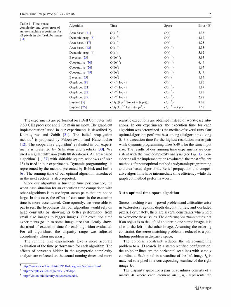
Table 1 summarizes the time–space complexity of several

classic stereo-matching methods. The area-based methods

have the best time performance and usually are referred to as

‘‘real-time’’ algorithms. Hence, area-based and dynamic

programming techniques are considered fast. Bayesian and

cooperative approaches have a good performance, while

graph cut and layered methods require much more resources.

The error column in Table 1 displays the gross error

evaluated for each method using the Tsukuba benchmark

data. These errors were reported in the old version of the

evaluation table in the Middlebury Stereo Vision website.1

The Tsukuba images are real stereo images with ground

truth obtained by manual annotation [31]. The area-based

methods and dynamic programming have reasonable

results in the [2.35%, 5.12%] error range. Bayesian and

Cooperative techniques have some of the best results in the

[1.15%, 6.49%] error range. Graph cut and layered

approaches perform very well concerning errors with

results in the [1.19%, 8.08%] error range.

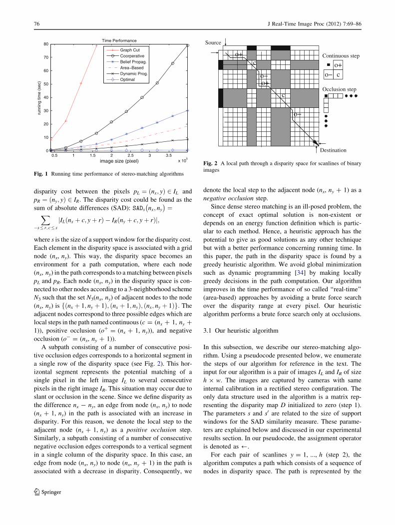
Here, we report the results of our experiments to com-

pare the running (execution) time performance of some

classic stereo-matching paradigms. The time performance

is evaluated by varying the size of the input images. The

input size ranges gradually from 40,000 pixels (i.e.,

200 9 200 image) to approximately 400,000 pixels (i.e.,

632 9 632 image). To obtain a specific dataset with uni-

formly distributed input sizes, the stereo pairs for the

running time experiments were synthetically generated

using a ray tracer.

1 http://vision.middlebury.edu/*schar/stereo/web/results.php.


123

http://vision.middlebury.edu/~schar/stereo/web/results.php

The experiments are performed on a Dell Computer with

2.80 GHz processor and 2 Gb main memory. The graph cut

implementation2 used in our experiments is described by

Kolmogorov and Zabih [21]. The belief propagation

method3 is proposed by Felzenszwalb and Huttenlocher

[12]. The cooperative algorithm4 evaluated in our experi-

ments is presented by Scharstein and Szeliski [30]. We

used a regular diffusion (with 80 iterations). An area-based

algorithm4 [1, 37] with shiftable square windows (of size

15) is used in our experiments. Dynamic programming4 is

represented by the method presented by Bobick and Intille

[6]. The running time of our optimal algorithm introduced

in the next section is also reported.

Since our algorithm is linear in time performance, the

worst-case situation for an execution time comparison with

other algorithms is to use input stereo pairs that are not so

large. In this case, the effect of constants in the execution

time is more accentuated. Consequently, we were able to

put to rest the hypothesis that our algorithm would rely on

huge constants by showing its better performance from

small size images to bigger images. Our execution time

experiments go up to some image size that clearly shows

the trend of execution time for each algorithm evaluated.

For all algorithms, the disparity range was adjusted

accordingly when necessary.

The running time experiments give a more accurate

evaluation of the time performance for each algorithm. The

effects of constants hidden in the asymptotic complexity

analysis are reflected on the actual running times and more

realistic executions are obtained instead of worst-case situ-

ations. In our experiments, the execution time for each

algorithm was determined as the median of several runs. Our

optimal algorithm performs best among all algorithms taking

0.43 s execution time for the highest resolution stereo pair

while dynamic programming takes 8.49 s for the same input

size. The results of our running time experiments are con-

sistent with the time complexity analysis (see Fig. 1). Con-

sidering all the implementations evaluated, the most efficient

methods after our optimal method are dynamic programming

and area-based algorithms. Belief propagation and cooper-

ative algorithms have intermediate time efficiency while the

graph cut method performs worst.

3 An optimal time–space algorithm

Stereo matching is an ill-posed problem and difficulties arise

in textureless regions, depth discontinuities, and occluded

pixels. Fortunately, there are several constraints which help

to overcome these issues. The ordering constraint states that

if an object is to the left of another in one stereo image, it is

also to the left in the other image. Assuming the ordering

constraint, the stereo-matching problem is reduced to a path

finding problem in disparity space.

The epipolar constraint reduces the stereo-matching

problem to a 1D search. In a stereo rectified configuration,

the epipolar lines are the horizontal scanlines with same y

coordinate. Each pixel in a scanline of the left image IL is

matched to a pixel in a corresponding scanline of the right

image IR.

The disparity space for a pair of scanlines consists of a

matrix M where each element M(nx, ny) represents the

Table 1 Time–space

complexity and gross error of

stereo-matching algorithms for

all pixels in the Tsukuba image

[31]

Algorithm Time Space Error (%)

Area-based [41] O(n1.5) O(n) 3.36

Dynamic prog. [6] O(n1.5) O(n) 4.12

Area-based [17] O(n1.5) O(n) 4.25

Area-based [42] O(n1.5) O(n1.5) 2.35

Dynamic prog. [4] O(n2) O(n) 5.12

Bayesian [23] O(kn1.5) O(n1.5) 3.95

Cooperative [30] O(kn1.5) O(n1.5) 6.49

Cooperative [26] O(kn2) O(n1.5) 1.67

Cooperative [49] O(kn2) O(n1.5) 3.49

Bayesian [35] O(kn2) O(n2) 1.15

Graph cut [8] Oðn3:5 log nÞ O(n) 1.86

Graph cut [21] Oðn4:5 log nÞ O(n1.5) 1.19



Layered [5] Oðk0ððk1n2:5 log nÞ þ ðk2nÞÞÞ O(n1.5) 8.08

Layered [25] Oðk0ðk1n3:5 log nþ k2n2ÞÞ O(n1.5 ? k2n) 1.58

2 http://www.cs.ucl.ac.uk/staff/V.Kolmogorov/software.html.3 http://people.cs.uchicago.edu/*pff/bp/.4 http://vision.middlebury.edu/stereo/code/.


123

http://www.cs.ucl.ac.uk/staff/V.Kolmogorov/software.html

http://people.cs.uchicago.edu/~pff/bp/

http://vision.middlebury.edu/stereo/code/

disparity cost between the pixels pL ¼ ðnx; yÞ 2 IL and

pR ¼ ðny; yÞ 2 IR: The disparity cost could be found as the

sum of absolute differences (SAD): SADs nx; ny

� �

¼X

�s� r; c� s

jILðnx þ c; yþ rÞ � IRðny þ c; yþ rÞj;

where s is the size of a support window for the disparity cost.

Each element in the disparity space is associated with a grid

node (nx, ny). This way, the disparity space becomes an

environment for a path computation, where each node

(nx, ny) in the path corresponds to a matching between pixels

pL and pR. Each node (nx, ny) in the disparity space is con-

nected to other nodes according to a 3-neighborhood scheme

N3 such that the set N3(nx, ny) of adjacent nodes to the node

(nx, ny) is fðnx þ 1; ny þ 1Þ; ðnx þ 1; nyÞ; ðnx; ny þ 1Þg: The

adjacent nodes correspond to three possible edges which are

local steps in the path named continuous (c = (nx ? 1, ny ?

1)), positive occlusion (o? = (nx ? 1, ny)), and negative

occlusion (o- = (nx, ny ? 1)).

A subpath consisting of a number of consecutive posi-

tive occlusion edges corresponds to a horizontal segment in

a single row of the disparity space (see Fig. 2). This hor-

izontal segment represents the potential matching of a

single pixel in the left image IL to several consecutive

pixels in the right image IR. This situation may occur due to

slant or occlusion in the scene. Since we define disparity as

the difference nx - ny, an edge from node (nx, ny) to node

(nx ? 1, ny) in the path is associated with an increase in

disparity. For this reason, we denote the local step to the

adjacent node (nx ? 1, ny) as a positive occlusion step.

Similarly, a subpath consisting of a number of consecutive

negative occlusion edges corresponds to a vertical segment

in a single column of the disparity space. In this case, an

edge from node (nx, ny) to node (nx, ny ? 1) in the path is

associated with a decrease in disparity. Consequently, we

denote the local step to the adjacent node (nx, ny ? 1) as a

negative occlusion step.

Since dense stereo matching is an ill-posed problem, the

concept of exact optimal solution is non-existent or

depends on an energy function definition which is partic-

ular to each method. Hence, a heuristic approach has the

potential to give as good solutions as any other technique

but with a better performance concerning running time. In

this paper, the path in the disparity space is found by a

greedy heuristic algorithm. We avoid global minimization

such as dynamic programming [34] by making locally

greedy decisions in the path computation. Our algorithm

improves in the time performance of so called ‘‘real-time’’

(area-based) approaches by avoiding a brute force search

over the disparity range at every pixel. Our heuristic

algorithm performs a brute force search only at occlusions.

3.1 Our heuristic algorithm

In this subsection, we describe our stereo-matching algo-

rithm. Using a pseudocode presented below, we enumerate

the steps of our algorithm for reference in the text. The

input for our algorithm is a pair of images IL and IR of size

h 9 w. The images are captured by cameras with same

internal calibration in a rectified stereo configuration. The

only data structure used in the algorithm is a matrix rep-

resenting the disparity map D initialized to zero (step 1).

The parameters s and s0 are related to the size of support

windows for the SAD similarity measure. These parame-

ters are explained below and discussed in our experimental

results section. In our pseudocode, the assignment operator

is denoted as /.

For each pair of scanlines y = 1, ..., h (step 2), the

algorithm computes a path which consists of a sequence of

nodes in disparity space. The path is represented by the

0.5 1 1.5 2 2.5 3 3.5x 10

5

0

10

20

30

40

50

60

70

80

image size (pixel)

runn

ing

time

(sec

)Time Performance

Graph CutCoorperativeBelief Propag.Area−BasedDynamic Prog.Optimal

Fig. 1 Running time performance of stereo-matching algorithms

o+co−

Continuous step

Occlusion step

Destination

Source

o−

o−o+

co+

c

Fig. 2 A local path through a disparity space for scanlines of binary

images


123

sequence of values the grid node (nx, ny) assumes in the

execution. The source node in the path is obtained by

searching the best match for the first pixel in both scan-

lines: (nx, 1) or (1, ny), where 1� nx; ny�w (steps 2.a–e).

This way, the path starts from either the left or top side of

the disparity space. A local step is performed until either

the bottom or right side of the disparity space is reached

(step 2.h). Hence, the destination node in the path is any

node representing a match for the last pixel in one of the

scanlines: (nx, w) or (w, ny), where 1� nx; ny�w:

Assuming the continuity constraint where the scene is

smooth almost everywhere, the ground truth path in dis-

parity space is connected. Hence, a feasible approach to

compute stereo matching is to perform a local search that

iteratively finds a heuristic path. At each iteration, the local

step is either a continuous step or a potential occlusion step

(positive or negative). The next node in the path is found as

the node with the minimum disparity cost in the 3-neigh-

borhood N3(nx, ny) of the current node (nx, ny). Therefore,

the next node in the path may represent a continuous match

(c = (nx ? 1, ny ? 1)) or a potential occlusion (o? =

(nx ? 1, ny) and o- = (nx, ny ? 1)). A potential occlusion

can be caused by an actual occlusion or a slanted patch

where one pixel in one image corresponds to more than one

pixel in the other image. Since continuity occurs almost

everywhere, a continuous match is preferred over any

potential occlusion. We favor continuous steps by repeating

the evaluation for a next node with a bigger support window

for the SAD disparity cost computation. This next node

evaluation is repeated until the next node with minimum

cost corresponds to a continuous step or the window size

reaches a limit s0 (steps 2.h.i–iii). Therefore, the next node

evaluation searches over a range ds = [1, s0] of correlation

window sizes, where s0 is the maximum size for a correla-

tion window. In this search, we compute the SAD disparity

cost for all the 3-neighbors in N3(nx, ny). If a potential

occlusion (o? or o-) is the neighbor with the minimum cost

for the current window size, the size of the window is

incremented and the next node evaluation continues at the

same current node. A continuous match happens when the

neighbor node with the minimum cost is the continuous

node (c = (nx ? 1, ny ? 1)). If the whole range of window

sizes is explored and a continuous match is not found, then

the best potential occlusion is selected as the local step.

The current number of consecutive potential occlusions

steps, positive and negative, is kept in the variables l? and

l-, respectively (steps 2.f–g and 2.h.iv–vi). These steps are

in the direction of increasing and decreasing disparities.

The only use of these counters, l? and l-, is to keep track

of the number of potential occlusion steps. If these numbers

reach a threshold l, the algorithm detects an actual occlu-

sion (instead of a slant) and performs a global search to find

the next disparity in the path. Hence, a global search in the

disparity range is performed when a certain maximum

number l of positive (negative) potential occlusion steps

are performed consecutively. This maximum number of

potential occlusion steps is related to the amount of dis-

parity difference expected in the scene for an occlusion.

For a current disparity node (nx, ny), a global search caused

by positive occlusion steps selects the node with the min-

imum disparity cost among all nodes (nx0 ny), where

nx0[ nx as the next node in the path (step 2.h.vii). Simi-

larly, a global search caused by negative occlusion steps

finds the node with the minimum disparity cost among all

nodes (nx ny0), where ny

0[ ny (step 2.h.viii). If the local

step is not an occlusion step, a continuous step is taken

(step 2.h.ix).

At each local step, the node (nx, ny) corresponds to a

match between a pixel (nx, y) in the left scanline and a pixel

(ny, y) in the right scanline, where y specifies the horizontal

scanlines in the pair of images. Using the left image as a

reference, the disparity of a pixel (nx, y) is nx - ny (step

2.h.x). The output of our algorithm is the disparity map D.

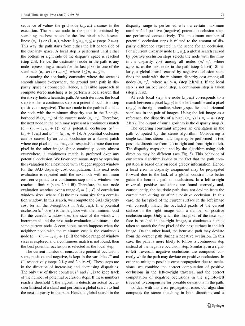
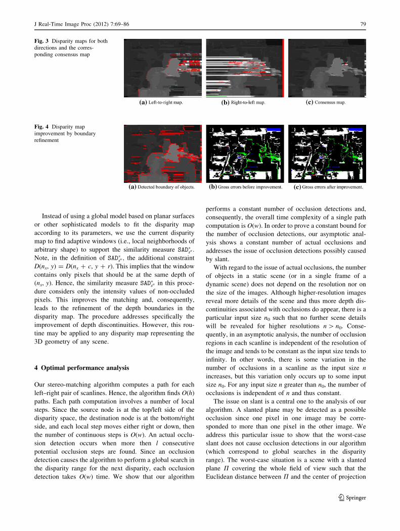
The ordering constraint imposes an orientation in the

path computed by the stereo algorithm. Considering a

single scanline, stereo matching may be performed in two

possible directions: from left to right and from right to left.

The disparity maps obtained by the algorithm using each

direction may be different (see Fig. 3). This behavior of

our stereo algorithm is due to the fact that the path com-

putation is based only on local greedy information. Hence,

a local error in disparity assignment may be propagated

forward due to the lack of a global constraint to better

guide the heuristic path on occlusions. In a left-to-right

traversal, positive occlusions are found correctly and,

consequently, the heuristic path does not deviate from the

correct path during or after a positive occlusion. In this

case, the last pixel of the current surface in the left image

will correctly match the occluded pixels of the current

surface in the right image with a number of positive

occlusion steps. Only when the first pixel of the next sur-

face is reached in the right image, a continuous step is

taken to match the first pixel of the next surface in the left

image. On the other hand, the heuristic path may deviate

from the correct path during a negative occlusion. In this

case, the path is more likely to follow a continuous step

instead of the negative occlusion step. Similarly, in a right-

to-left traversal, negative occlusions are computed cor-

rectly while the path may deviate on positive occlusions. In

order to mitigate possible error propagation due to occlu-

sions, we combine the correct computation of positive

occlusions in the left-to-right traversal and the correct

computation of negative occlusions in the right-to-left

traversal to compensate for possible deviations in the path.

To deal with this error propagation issue, our algorithm

computes the stereo matching in both directions and a


123

consensus routine produces a single map from the two

results. Our consensus routine exploits constraint propa-

gation between adjacent scanlines to find a disparity based

on statistics of a neighborhood region surrounding a par-

ticular pixel. The procedure assigns to each pixel the

median disparity of both neighborhoods in the left-to-right

and right-to-left maps corresponding to the same pixel.

Formally, given the left-to-right disparity map DL2R and the

right-to-left disparity map DR2L, the consensus disparity

map D is obtained such that D(nx, y) is the median of the

disparity set S(nx, y), where Sðnx; yÞ ¼S

�s� r;c� s fDL2R

ðnx þ r; yþ cÞ; DR2Lðnx þ r; yþ cÞg and s is a window size

representing pixel neighborhood.

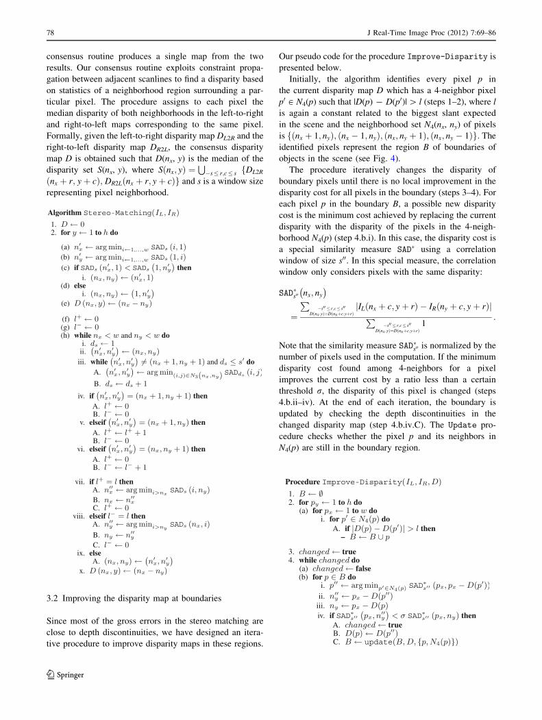
3.2 Improving the disparity map at boundaries

Since most of the gross errors in the stereo matching are

close to depth discontinuities, we have designed an itera-

tive procedure to improve disparity maps in these regions.

Our pseudo code for the procedure Improve-Disparity is

presented below.

Initially, the algorithm identifies every pixel p in

the current disparity map D which has a 4-neighbor pixel

p0 [ N4(p) such that |D(p) - D(p0)| [ l (steps 1–2), where l

is again a constant related to the biggest slant expected

in the scene and the neighborhood set N4(nx, ny) of pixels

is fðnx þ 1; nyÞ; ðnx � 1; nyÞ; ðnx; ny þ 1Þ; ðnx; ny � 1Þg: The

identified pixels represent the region B of boundaries of

objects in the scene (see Fig. 4).

The procedure iteratively changes the disparity of

boundary pixels until there is no local improvement in the

disparity cost for all pixels in the boundary (steps 3–4). For

each pixel p in the boundary B, a possible new disparity

cost is the minimum cost achieved by replacing the current

disparity with the disparity of the pixels in the 4-neigh-

borhood N4(p) (step 4.b.i). In this case, the disparity cost is

a special similarity measure SAD� using a correlation

window of size s00. In this special measure, the correlation

window only considers pixels with the same disparity:

SAD�s00 nx; ny

� �

¼

P

�s00 � r;c� s00Dðnx ;yÞ¼Dðnxþc;yþrÞ

jILðnx þ c; yþ rÞ � IRðny þ c; yþ rÞjP

�s00 � r;c� s00Dðnx ;yÞ¼Dðnxþc;yþrÞ

1:

Note that the similarity measure SAD�s00 is normalized by the

number of pixels used in the computation. If the minimum

disparity cost found among 4-neighbors for a pixel

improves the current cost by a ratio less than a certain

threshold r, the disparity of this pixel is changed (steps

4.b.ii–iv). At the end of each iteration, the boundary is

updated by checking the depth discontinuities in the

changed disparity map (step 4.b.iv.C). The Update pro-

cedure checks whether the pixel p and its neighbors in

N4(p) are still in the boundary region.


123

Instead of using a global model based on planar surfaces

or other sophisticated models to fit the disparity map

according to its parameters, we use the current disparity

map to find adaptive windows (i.e., local neighborhoods of

arbitrary shape) to support the similarity measure SAD�s00 :Note, in the definition of SAD�s00 ; the additional constraint

D(nx, y) = D(nx ? c, y ? r). This implies that the window

contains only pixels that should be at the same depth of

(nx, y). Hence, the similarity measure SAD�s00 in this proce-

dure considers only the intensity values of non-occluded

pixels. This improves the matching and, consequently,

leads to the refinement of the depth boundaries in the

disparity map. The procedure addresses specifically the

improvement of depth discontinuities. However, this rou-

tine may be applied to any disparity map representing the

3D geometry of any scene.

4 Optimal performance analysis

Our stereo-matching algorithm computes a path for each

left–right pair of scanlines. Hence, the algorithm finds O(h)

paths. Each path computation involves a number of local

steps. Since the source node is at the top/left side of the

disparity space, the destination node is at the bottom/right

side, and each local step moves either right or down, then

the number of continuous steps is O(w). An actual occlu-

sion detection occurs when more then l consecutive

potential occlusion steps are found. Since an occlusion

detection causes the algorithm to perform a global search in

the disparity range for the next disparity, each occlusion

detection takes O(w) time. We show that our algorithm

performs a constant number of occlusion detections and,

consequently, the overall time complexity of a single path

computation is O(w). In order to prove a constant bound for

the number of occlusion detections, our asymptotic anal-

ysis shows a constant number of actual occlusions and

addresses the issue of occlusion detections possibly caused

by slant.

With regard to the issue of actual occlusions, the number

of objects in a static scene (or in a single frame of a

dynamic scene) does not depend on the resolution nor on

the size of the images. Although higher-resolution images

reveal more details of the scene and thus more depth dis-

continuities associated with occlusions do appear, there is a

particular input size n0 such that no further scene details

will be revealed for higher resolutions n [ n0. Conse-

quently, in an asymptotic analysis, the number of occlusion

regions in each scanline is independent of the resolution of

the image and tends to be constant as the input size tends to

infinity. In other words, there is some variation in the

number of occlusions in a scanline as the input size n

increases, but this variation only occurs up to some input

size n0. For any input size n greater than n0, the number of

occlusions is independent of n and thus constant.

The issue on slant is a central one to the analysis of our

algorithm. A slanted plane may be detected as a possible

occlusion since one pixel in one image may be corre-

sponded to more than one pixel in the other image. We

address this particular issue to show that the worst-case

slant does not cause occlusion detections in our algorithm

(which correspond to global searches in the disparity

range). The worst-case situation is a scene with a slanted

plane P covering the whole field of view such that the

Euclidean distance between P and the center of projection

Fig. 3 Disparity maps for both

directions and the corres-

ponding consensus map

Fig. 4 Disparity map

improvement by boundary

refinement


123

pL of the left camera in 3D space is a very small �[ 0: In

this case, the slanted plane almost passes through the

camera center. Note that in the degenerate case where the

slanted plane P contains the center of projection pL (i.e.,

� ¼ 0:), the points in the plane will be projected into a

straight line in the left camera. Hence, the pixels in a

particular scanline of the right image correspond to the

same single pixel in the left image. We assume �[ d,

where d is a constant number that bounds the minimum

distance between the plane P and the center of the camera.

As a consequence, the constant d bounds the maximum

slope of the plane P. The constant d allows a big range of

planar slant but avoids planes infinitely close to pL. This

assumption of our algorithm is based on the disparity

gradient limit constraint [9]. This constraint assumes that

disparity does not change too rapidly with space. In other

words, humans are not able to perceive depth when dis-

parity changes abruptly. This is considered in our algorithm

by assuming the constant d which bounds the maximum

slant and, consequently, bounds the maximum change of

disparity: a limited gradient for disparity.

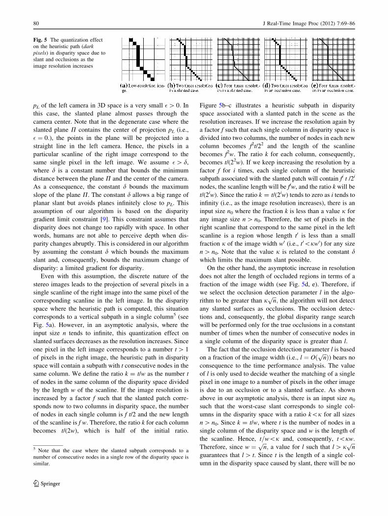
Even with this assumption, the discrete nature of the

stereo images leads to the projection of several pixels in a

single scanline of the right image into the same pixel of the

corresponding scanline in the left image. In the disparity

space where the heuristic path is computed, this situation

corresponds to a vertical subpath in a single column5 (see

Fig. 5a). However, in an asymptotic analysis, where the

input size n tends to infinite, this quantization effect on

slanted surfaces decreases as the resolution increases. Since

one pixel in the left image corresponds to a number t [ 1

of pixels in the right image, the heuristic path in disparity

space will contain a subpath with t consecutive nodes in the

same column. We define the ratio k = t/w as the number t

of nodes in the same column of the disparity space divided

by the length w of the scanline. If the image resolution is

increased by a factor f such that the slanted patch corre-

sponds now to two columns in disparity space, the number

of nodes in each single column is f t/2 and the new length

of the scanline is f w. Therefore, the ratio k for each column

becomes t/(2w), which is half of the initial ratio.

Figure 5b–c illustrates a heuristic subpath in disparity

space associated with a slanted patch in the scene as the

resolution increases. If we increase the resolution again by

a factor f such that each single column in disparity space is

divided into two columns, the number of nodes in each new

column becomes f2t/22 and the length of the scanline

becomes f2w. The ratio k for each column, consequently,

becomes t/(22w). If we keep increasing the resolution by a

factor f for i times, each single column of the heuristic

subpath associated with the slanted patch will contain fi t /2i

nodes, the scanline length will be fiw, and the ratio k will be

t/(2iw). Since the ratio k = t/(2iw) tends to zero as i tends to

infinity (i.e., as the image resolution increases), there is an

input size n0 where the fraction k is less than a value j for

any image size n [ n0. Therefore, the set of pixels in the

right scanline that correspond to the same pixel in the left

scanline is a region whose length t0 is less than a small

fraction j of the image width w0 (i.e., t0\jw0) for any size

n [ n0. Note that the value j is related to the constant dwhich limits the maximum slant possible.

On the other hand, the asymptotic increase in resolution

does not alter the length of occluded regions in terms of a

fraction of the image width (see Fig. 5d, e). Therefore, if

we select the occlusion detection parameter l in the algo-

rithm to be greater than jffiffiffi

np

; the algorithm will not detect

any slanted surfaces as occlusions. The occlusion detec-

tions and, consequently, the global disparity range search

will be performed only for the true occlusions in a constant

number of times when the number of consecutive nodes in

a single column of the disparity space is greater than l.

The fact that the occlusion detection parameter l is based

on a fraction of the image width (i.e., l ¼ Oðffiffiffi

npÞ) bears no

consequence to the time performance analysis. The value

of l is only used to decide weather the matching of a single

pixel in one image to a number of pixels in the other image

is due to an occlusion or to a slanted surface. As shown

above in our asymptotic analysis, there is an input size n0

such that the worst-case slant corresponds to single col-

umns in the disparity space with a ratio k\j for all sizes

n [ n0. Since k = t/w, where t is the number of nodes in a

single column of the disparity space and w is the length of

the scanline. Hence, t=w\j and, consequently, t\jw:

Therefore, since w ¼ffiffiffi

np

; a value for l such that l [ jffiffiffi

np

guarantees that l [ t. Since t is the length of a single col-

umn in the disparity space caused by slant, there will be no

Fig. 5 The quantization effect

on the heuristic path (darkpixels) in disparity space due to

slant and occlusions as the

image resolution increases

5 Note that the case where the slanted subpath corresponds to a

number of consecutive nodes in a single row of the disparity space is

similar.


123

false occlusion detections due to slant. Hence, slant has no

impact in the time complexity of the algorithm, since no

occlusion detections will be caused by slant and, conse-

quently, the number of occlusion detections in our algo-

rithm is still constant (only due to legitimate occlusions).

Overall, a path computation performs O(w) continuous

steps in constant time and a constant number of searches in

the disparity range, each search in O(w) time. Hence, each

path is found in O(w) time and the stereo-matching algo-

rithm takes O(hw) = O(n) time for all h scanlines. An

iteration of the improving disparity procedure updates the

disparity of each boundary pixel in constant time. Since the

number of objects in the scene is constant (i.e., independent

of the size of the image), the number of pixels in the

boundary region is O(h ? w) and, consequently, a disparity

update iteration takes O(n0.5) time. A disparity update

represents a move of the boundary region towards its

correct location. Since the maximum displacement of a

boundary pixel is O(h ? w) pixels, the maximum number

of iterations towards the correct boundary is O(n0.5).

Therefore, the improving stereo algorithm takes O(n) time.

The stereo-matching algorithm requires O(n) space for

the disparity map. The improving stereo procedure keeps

the boundary region in a list of pixels which requires

O(h ? w) space. Other data structures used in the procedure

have the same size as a disparity map. Hence, the improving

stereo procedure also requires linear space. Therefore, our

method is linear in time and space complexity. Since the

linear size of the output (disparity map) is a lower bound for

the stereo-matching problem, our algorithm is optimal

concerning time and space requirements.

5 Experimental results

A heuristic path in disparity space most likely will not be

the best path associated with the true matchings between

pixels in corresponding scanlines. However, no technique

guarantees to find such a best path due to the ill-posed

nature of the stereo-matching problem. Even global tech-

niques such as dynamic programming cannot guarantee

that the ground truth will be found. A global approach only

finds the path with minimum cost according to some

matching cost function modeling the problem. The only

way to evaluate the correctness of a stereo-matching

algorithm is through its implementation and by performing

experiments with ground truth data.

Our stereo-matching algorithm was implemented and

some experimentation was performed initially to obtain

reasonable values for some parameters. The parameters

considered include the maximum size s0 of a correlation

window used to decide on taking a potential positive and

negative occlusion step, the number l of successive

potential occlusions which defines a candidate occlusion,

the size s00 of the window for the special SAD used in the

improving algorithm, and the associated ratio threshold rin the improving stereo routine.

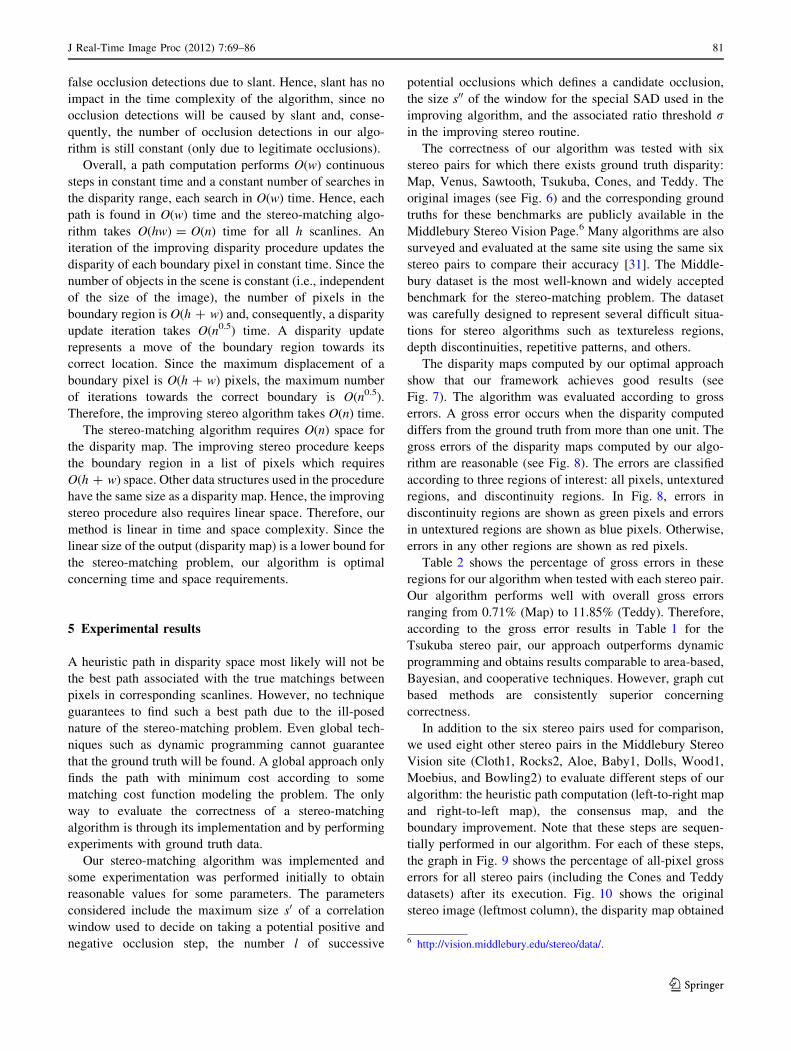
The correctness of our algorithm was tested with six

stereo pairs for which there exists ground truth disparity:

Map, Venus, Sawtooth, Tsukuba, Cones, and Teddy. The

original images (see Fig. 6) and the corresponding ground

truths for these benchmarks are publicly available in the

Middlebury Stereo Vision Page.6 Many algorithms are also

surveyed and evaluated at the same site using the same six

stereo pairs to compare their accuracy [31]. The Middle-

bury dataset is the most well-known and widely accepted

benchmark for the stereo-matching problem. The dataset

was carefully designed to represent several difficult situa-

tions for stereo algorithms such as textureless regions,

depth discontinuities, repetitive patterns, and others.

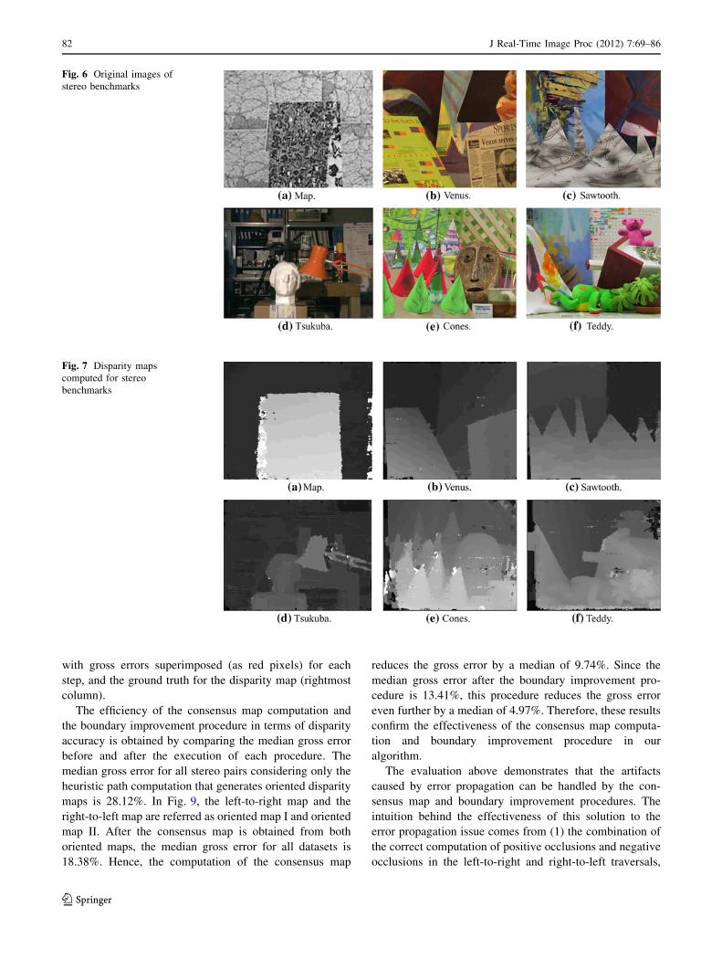
The disparity maps computed by our optimal approach

show that our framework achieves good results (see

Fig. 7). The algorithm was evaluated according to gross

errors. A gross error occurs when the disparity computed

differs from the ground truth from more than one unit. The

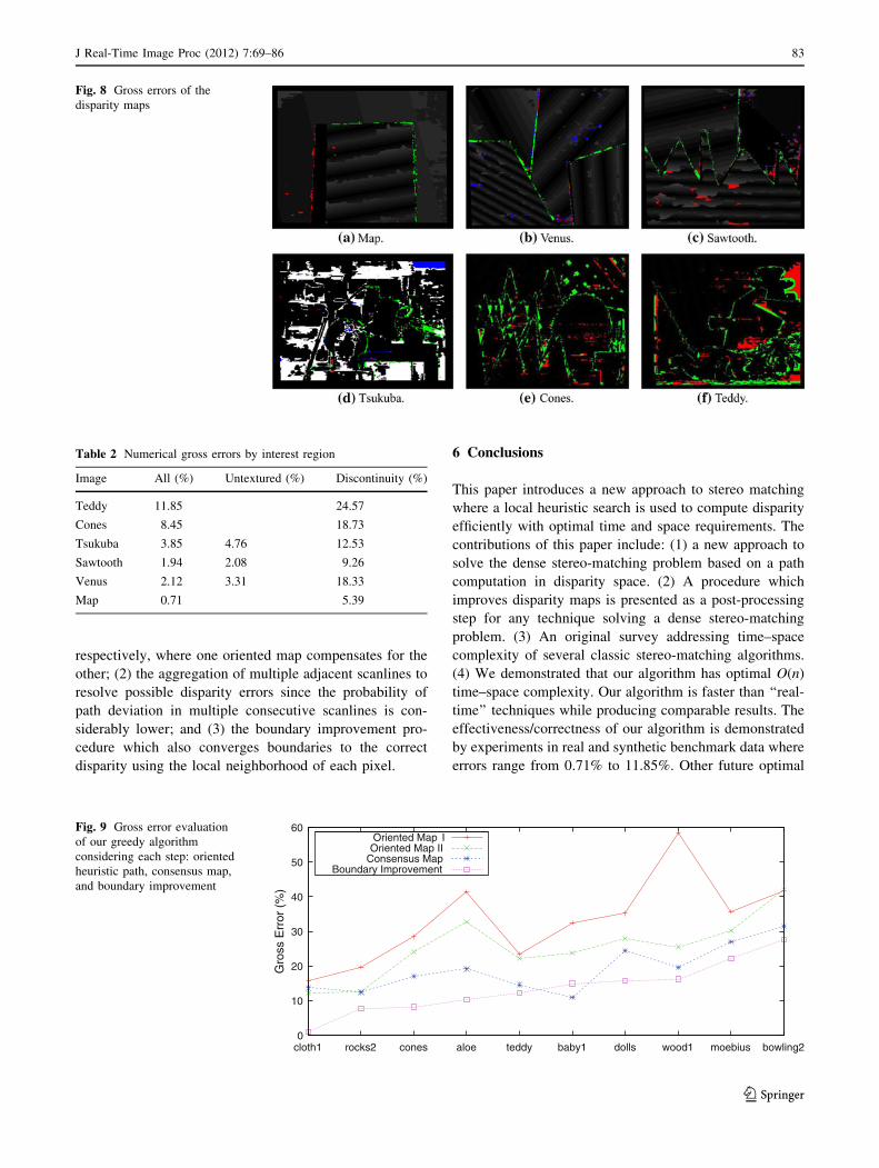
gross errors of the disparity maps computed by our algo-

rithm are reasonable (see Fig. 8). The errors are classified

according to three regions of interest: all pixels, untextured

regions, and discontinuity regions. In Fig. 8, errors in

discontinuity regions are shown as green pixels and errors

in untextured regions are shown as blue pixels. Otherwise,

errors in any other regions are shown as red pixels.

Table 2 shows the percentage of gross errors in these

regions for our algorithm when tested with each stereo pair.

Our algorithm performs well with overall gross errors

ranging from 0.71% (Map) to 11.85% (Teddy). Therefore,

according to the gross error results in Table 1 for the

Tsukuba stereo pair, our approach outperforms dynamic

programming and obtains results comparable to area-based,

Bayesian, and cooperative techniques. However, graph cut

based methods are consistently superior concerning

correctness.

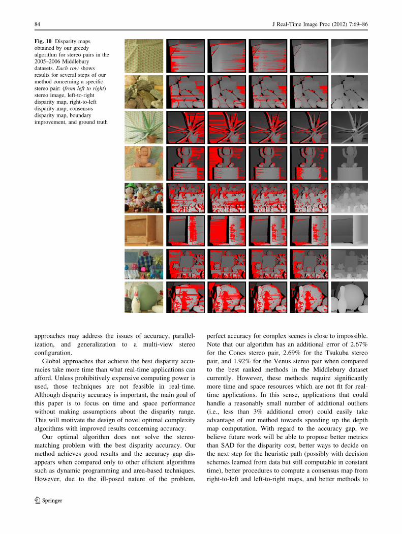
In addition to the six stereo pairs used for comparison,

we used eight other stereo pairs in the Middlebury Stereo

Vision site (Cloth1, Rocks2, Aloe, Baby1, Dolls, Wood1,

Moebius, and Bowling2) to evaluate different steps of our

algorithm: the heuristic path computation (left-to-right map

and right-to-left map), the consensus map, and the

boundary improvement. Note that these steps are sequen-

tially performed in our algorithm. For each of these steps,

the graph in Fig. 9 shows the percentage of all-pixel gross

errors for all stereo pairs (including the Cones and Teddy

datasets) after its execution. Fig. 10 shows the original

stereo image (leftmost column), the disparity map obtained

6 http://vision.middlebury.edu/stereo/data/.


123

http://vision.middlebury.edu/stereo/data/

with gross errors superimposed (as red pixels) for each

step, and the ground truth for the disparity map (rightmost

column).

The efficiency of the consensus map computation and

the boundary improvement procedure in terms of disparity

accuracy is obtained by comparing the median gross error

before and after the execution of each procedure. The

median gross error for all stereo pairs considering only the

heuristic path computation that generates oriented disparity

maps is 28.12%. In Fig. 9, the left-to-right map and the

right-to-left map are referred as oriented map I and oriented

map II. After the consensus map is obtained from both

oriented maps, the median gross error for all datasets is

18.38%. Hence, the computation of the consensus map

reduces the gross error by a median of 9.74%. Since the

median gross error after the boundary improvement pro-

cedure is 13.41%, this procedure reduces the gross error

even further by a median of 4.97%. Therefore, these results

confirm the effectiveness of the consensus map computa-

tion and boundary improvement procedure in our

algorithm.

The evaluation above demonstrates that the artifacts

caused by error propagation can be handled by the con-

sensus map and boundary improvement procedures. The

intuition behind the effectiveness of this solution to the

error propagation issue comes from (1) the combination of

the correct computation of positive occlusions and negative

occlusions in the left-to-right and right-to-left traversals,

Fig. 6 Original images of

stereo benchmarks

Fig. 7 Disparity maps

computed for stereo

benchmarks


123

respectively, where one oriented map compensates for the

other; (2) the aggregation of multiple adjacent scanlines to

resolve possible disparity errors since the probability of

path deviation in multiple consecutive scanlines is con-

siderably lower; and (3) the boundary improvement pro-

cedure which also converges boundaries to the correct

disparity using the local neighborhood of each pixel.

6 Conclusions

This paper introduces a new approach to stereo matching

where a local heuristic search is used to compute disparity

efficiently with optimal time and space requirements. The

contributions of this paper include: (1) a new approach to

solve the dense stereo-matching problem based on a path

computation in disparity space. (2) A procedure which

improves disparity maps is presented as a post-processing

step for any technique solving a dense stereo-matching

problem. (3) An original survey addressing time–space

complexity of several classic stereo-matching algorithms.

(4) We demonstrated that our algorithm has optimal O(n)

time–space complexity. Our algorithm is faster than ‘‘real-

time’’ techniques while producing comparable results. The

effectiveness/correctness of our algorithm is demonstrated

by experiments in real and synthetic benchmark data where

errors range from 0.71% to 11.85%. Other future optimal

Fig. 8 Gross errors of the

disparity maps

Table 2 Numerical gross errors by interest region

Image All (%) Untextured (%) Discontinuity (%)

Teddy 11.85 24.57

Cones 8.45 18.73

Tsukuba 3.85 4.76 12.53

Sawtooth 1.94 2.08 9.26

Venus 2.12 3.31 18.33

Map 0.71 5.39

0

10

20

30

40

50

60

cloth1 rocks2 cones aloe teddy baby1 dolls wood1 moebius bowling2

Gro

ss E

rror

(%

)

Oriented Map IOriented Map II

Consensus MapBoundary Improvement

Fig. 9 Gross error evaluation

of our greedy algorithm

considering each step: oriented

heuristic path, consensus map,

and boundary improvement


123

approaches may address the issues of accuracy, parallel-

ization, and generalization to a multi-view stereo

configuration.

Global approaches that achieve the best disparity accu-

racies take more time than what real-time applications can

afford. Unless prohibitively expensive computing power is

used, those techniques are not feasible in real-time.

Although disparity accuracy is important, the main goal of

this paper is to focus on time and space performance

without making assumptions about the disparity range.

This will motivate the design of novel optimal complexity

algorithms with improved results concerning accuracy.

Our optimal algorithm does not solve the stereo-

matching problem with the best disparity accuracy. Our

method achieves good results and the accuracy gap dis-

appears when compared only to other efficient algorithms

such as dynamic programming and area-based techniques.

However, due to the ill-posed nature of the problem,

perfect accuracy for complex scenes is close to impossible.

Note that our algorithm has an additional error of 2.67%

for the Cones stereo pair, 2.69% for the Tsukuba stereo

pair, and 1.92% for the Venus stereo pair when compared

to the best ranked methods in the Middlebury dataset

currently. However, these methods require significantly

more time and space resources which are not fit for real-

time applications. In this sense, applications that could

handle a reasonably small number of additional outliers

(i.e., less than 3% additional error) could easily take

advantage of our method towards speeding up the depth

map computation. With regard to the accuracy gap, we

believe future work will be able to propose better metrics

than SAD for the disparity cost, better ways to decide on

the next step for the heuristic path (possibly with decision

schemes learned from data but still computable in constant

time), better procedures to compute a consensus map from

right-to-left and left-to-right maps, and better methods to

Fig. 10 Disparity maps

obtained by our greedy

algorithm for stereo pairs in the

2005–2006 Middlebury

datasets. Each row shows

results for several steps of our

method concerning a specific

stereo pair: (from left to right)stereo image, left-to-right

disparity map, right-to-left

disparity map, consensus

disparity map, boundary

improvement, and ground truth


123

handle occlusions and avoid path deviation or error

propagation.

Another relevant issue related to depth maps from stereo

data is that the precision in 3D space deteriorates with

increasing distance from the camera. One possible way to

handle this is to use sub-pixel optimization. However, this

relies on models that may not be true and, hence, result in

poor precision. On the other hand, high-resolution images

retrieve more information from the scene to be used on the

computation of 3D geometry. A real-time algorithm allows

applications to handle high-resolution images. In other

words, in the same time period, a real-time method handles

more pixels. Since precision in 3D space strongly depends

on the resolution of the cameras, a real-time method allows

better precision. Therefore, a significantly bigger number

of more precise inlier disparities compensates for the

additional outliers that resulted from the disparity errors of

our real-time algorithm. In a nutshell, the improved pre-

cision in 3D space that results from a high-resolution dis-

parity map is a significant gain even when contrasted with

the small number of additional disparity errors. In this

sense, the ability to handle super-resolution images in real-

time is of crucial importance. A new ranking based on the

time and space performance of stereo algorithms is needed.

This ranking will have a tremendous impact on the efforts

to improve the precision of reconstructed 3D geometry.

We should state that our survey addressing space–time

complexity focus only on sequential algorithms. We rec-

ognize the relevance of parallel algorithms to real-time

applications. Although parallel algorithms require more

computing resources, they achieve significantly better

processing times. Due to the importance of time efficiency

to real-time applications using stereo matching, we foresee

the need for a survey of parallel stereo-matching algo-

rithms with complexity analysis and uniform experiments

on execution time.

A parallel version of our algorithm is a possible direction

for future work. We also anticipate a generalization of our

technique to multi-view stereo matching. For a regular grid

of cameras, this generalization will be used to further

improve accuracy and boundary artifacts. The algorithm will

have to consider multiple potential occlusions between dif-

ferent pairs of images in the grid. In this case, a local step in

disparity space will involve 2i - 1 possibilities, where i is

the number of stereo images from the camera grid. For a

general configuration of multiple cameras, once the funda-

mental matrices are inferred from a sparse set of features in

all images, our algorithm may be generalized to find dense

matchings between corresponding epipolar lines. Finally,

the use of our algorithm in the motion field computation is

also feasible when the ordering constraint is generalized and

linearization is applied in the 2D disparity space.

References

1. Arnold, R.: Automated stereo perception. PhD thesis, memo

AIM-351 (1983)

2. Belhumeur, P.: A Bayesian approach to binocular stereopsis. Int.

J. Comput. Vis. 19(3), 237–260 (1996)

3. Belhumeur, P., Mumford, D.A.: Bayesian treatment of the stereo

correspondence problem using half-occluded region. In: Pro-

ceedings of the Conference on Computer Vision and Pattern

Recognition, pp. 506–512 (1992)

4. Birchfield, S., Tomasi, C.: Depth discontinuities by pixel-to-pixel

stereo. In: Proceedings of the International Conference on

Computer Vision, pp. 1073–1080 (1998)

5. Birchfield, S., Tomasi, C.: Multiway cut for stereo and motion

with slanted surfaces. In: Proceedings of the International Con-

ference on Computer Vision, pp. 489–495 (1999)

6. Bobick, A., Intille, S.: Large occlusion stereo. Int. J. Comput. Vis.

33(3), 181–200 (1999)

7. Boykov, Y., Veksler, O., Zabih, R.: Markov random fields with

efficient approximations. In: Proceedings of the Conference on

Computer Vision and Pattern Recognition, pp. 648–655 (1998)

8. Boykov, Y., Veksler, O., Zabih, R.: Fast approximate energy

minimization via graph cuts. IEEE Trans. Pattern Anal. Mach.

Intell. 23(11), 1222–1239 (2001)

9. Burt, P., Julesz, B.: A disparity gradient limit for binocular

fusion. Perception 9, 671–682 (1980)

10. Collins, R.: A space-sweep approach to true multi-image

matching. In: Proceedings of the Conference on Computer Vision

and Pattern Recognition, pp. 358–363 (1996)

11. Criminisi, A., Blake, A., Rother, C., Shotton, J., Torr, P.: Efficient

dense stereo with occlusions for new view-synthesis by four-state

dynamic programming. Int. J. Comput. Vis. 71(1), 89–110 (2007)

12. Felzenszwalb, P., Huttenlocher, D.: Efficient belief propagation

for early vision. In: Proceedings of the Conference on Computer

Vision and Pattern Recognition, pp. 261–268 (2004)

13. Gallup, D., Frahm, J.M., Mordohai, P., Pollefeys, M.: Variable

baseline/resolution stereo. In: Proceedings of the Conference on


14. Gill, P., Leonard, M.: Reduced-Hessian quasi-Newton methods for

unconstrained optimization. SIAM J. Optim. 12(1), 209–237

(2001)

15. Goldberg, A., Tarjan, R.: A new approach to the maximum-flow

problem. J. ACM 35(4), 921–940 (1988)

16. Gong, M., Yang, Y.H.: Near real-time reliable stereo matching

using programmable graphics. In: Proceedings of the Conference

on Computer Vision and Pattern Recognition, pp. 924–931 (2005)

17. Hirschmuller, H.: Improvements in real-time correlation-based

stereo vision. In: Proceedings of the Workshop on Stereo and

Multi-Baseline Vision, pp. 141–148 (2001)

18. Hirschmuller, H.: Stereo processing by semi-global matching and

mutual information. IEEE Trans. Pattern Anal. Mach. Intell.

30(2), 328–341 (2008)

19. Kanade, T., Okutomi, M.: A stereo matching algorithm with an

adaptive window: theory and experiment. IEEE Trans. Pattern

Anal. Mach. Intell. 16(9), 920–932 (1994)

20. Klaus, A., Sormann, M., Karner, K.: Segment-based stereo

matching using belief propagation and a self-adapting dissimi-

larity measure. In: Proceedings of the International Conference

on Pattern Recognition, pp. 15–18 (2006)

21. Kolmogorov, V., Zabih, R.: Computing visual correspondence

with occlusions using graph cuts. In: Proceedings of the Inter-

national Conference on Computer Vision, pp. 508–515 (2001)

22. Kolmogorov, V., Zabih, R.: Multi-camera scene reconstruction

via graph cuts. In: Proceedings of the European Conference on

Computer Vision, pp. 82–96 (2002)


123

23. Lee, S., Kanatsugu, Y., Park, J.I.: Hierarchical stochastic diffu-

sion for disparity estimation. In: Proceedings of the Workshop on

Stereo and Multi-Baseline Vision, pp. 111–120 (2001)

24. Levine, M., O’Handley, D., Yagi, G.: Computer determination of

depth maps. Comput. Graph. Image Process. 2, 131–150 (1973)

25. Lin, M., Tomasi, C.: Surfaces with occlusions from layered ste-

reo. In: Proceedings of the Conference on Computer Vision and

Pattern Recognition, pp. 710–717 (2003)

26. Mayer, H.: Analysis of means to improve cooperative disparity

estimation. In: Proceedings of the ISPRS Conference on Photo-

grammetric Image Analysis (2003)

27. Mori, K., Kidode, M., Asada, H.: An iterative prediction and

correction method for automatic stereocomparison Comput.

Graph. Image Process. 2, 393–401 (1973)

28. Rother, C., Kolmogorov, V., Lempitsky, V., Szummer, M.:

Optimizing binary MRFs via extended roof duality. In: Pro-

ceedings of the Conference on Computer Vision and Pattern

Recognition, pp. 1–8 (2007)

29. Roy, S., Cox, I.: A maximum-flow formulation of the N-camera

stereo correspondence problem. In: Proceedings of the Interna-

tional Conference on Computer Vision, pp. 492–499 (1998)

30. Scharstein, D., Szeliski, R.: Stereo matching with non-linear

diffusion. Int. J. Comput. Vis. 28(2), 155–174 (1998)

31. Scharstein, D., Szeliski, R.: A taxonomy and evaluation of dense

two-frame stereo correspondence algorithms. Int. J. Comput. Vis.

47(1-3), 7–42 (2002)

32. Shi, J., Tomasi, C.: Good features to track. In: Proceedings of the

Conference on Computer Vision and Pattern Recognition, pp.

593–600 (1994)

33. Strecha, C., Fransens, R., Gool, L.V.: Combined depth and outlier

estimation in multi-view stereo. In: Proceedings of the Confer-

ence on Computer Vision and Pattern Recognition, pp. 2394–

2401 (2006)

34. Sun, C.: Multi-resolution stereo matching using maximum-sur-

face techniques. In: Proceedings of the Digital Image Computing:

Techniques and Applications, pp. 195–200 (1999)

35. Sun, J., Zheng, N.N., Shum, H.Y.: Stereo matching using belief

propagation. IEEE Trans. Pattern Anal. Mach. Intell. 25(7), 787–

800 (2003)

36. Sun, J., Li, Y., Kang, S., Shum, H.Y.: Symmetric stereo matching

for occlusion handling. In: Proceedings of the Conference on


37. Tao, H., Sawhney, H., Kumar, R.: A global matching framework

for stereo computation. In: Proceedings of the International

Conference on Computer Vision, pp. 532–539 (2001)

38. Tombari, F., Mattoccia, S., Stefano, L.D.: Segmentation-based

adaptive support for accurate stereo correspondence. In: Advan-

ces in Image and Video Technology, Springer, Lecture Notes in

Computer Science, vol. 4872, pp. 427–438 (2007)

39. Torr, P., Criminisi, A.: Dense stereo using pivoted dynamic

programming. Image Vis. Comput. 22(10), 795–806 (2004)

40. Veksler, O.: Efficient graph-based energy minimization methods

in computer vision. PhD thesis, Department of Computer Sci-

ence, Cornell University (1999)

41. Veksler, O.: Stereo correspondence with compact windows via

minimum ratio cycle. IEEE Trans. Pattern Anal. Mach. Intell.

24(12), 1654–1660 (2002)

42. Veksler, O.: Fast variable window for stereo correspondence

using integral images. In: Proceedings of the Conference on


43. Veksler, O.: Stereo correspondence by dynamic programming on

a tree. In: Proceedings of the Conference on Computer Vision and

Pattern Recognition, pp. 384–390 (2005)

44. Wang, L., Liao, M., Gong, M., Yang, R., Nister, D.: High-quality

real-time stereo using adaptive cost aggregation and dynamic

programming. In: Proceedings of the International Symposium on

3D Data Processing, Visualization, and Transmission, pp. 798–

805 (2006)

45. Woodford, O., Torr, P., Reid, I., Fitzgibbon, A.: Global stereo

reconstruction under second order smoothness priors. IEEE

Trans. Pattern Anal. Mach. Intell. 31(12), 2115–2128 (2009)

46. Yang, Q., Wang, L., Yang, R., Stewenius, H., Nister, D.: Stereo

matching with color-weighted correlation, hierarchical belief

propagation, and occlusion handling. IEEE Trans. Pattern Anal.

Mach. Intell. 31(3), 492–504 (2009)

47. Yang, R., Pollefeys, M.: Multi-resolution real-time stereo on

commodity graphics hardware. In: Proceedings of the Conference

on Computer Vision and Pattern Recognition, pp. 211–217

(2003)

48. Yoon, K.J., Kweon, I.: Adaptive support-weight approach for

correspondence search. IEEE Trans. Pattern Anal. Mach. Intell.

28(4), 650–656 (2006)

49. Zitnick, C., Kanade, T.: A cooperative algorithm for stereo

matching and occlusion detection. IEEE Trans. Pattern Anal.

Mach. Intell. 22(7), 675–684 (2000)

50. Zitnick, C., Kang, S.: Stereo for image-based rendering using

image over-segmentation. Int. J. Comput. Vis. 75(1), 49–65

(2007)

Author Biography

Gutemberg Guerra-Filho is an assistant professor in the Computer

Science and Engineering Department at the University of Texas at

Arlington. He received his PhD degree in Computer Science from the

University of Maryland, College Park, in 2007 as a member of the

Computer Vision Laboratory. He has a MSc degree in Computer

Science from the University of Maryland and another from the State

University of Campinas, Brazil, in 2006 and 1998, respectively. His

current research involves the development of sensory-motor lan-

guages for artificial cognitive systems. This linguistic learning

framework has applications in Computer Vision and Graphics,

Humanoid Robotics, Multi-Modal Multimedia, Data Mining, and

Artificial Intelligence. His other research interests are Computational

Geometry, Spatial Databases, and Combinatorial Optimization.


123

an optimal time–space algorithm for dense stereo matching

Documents