an optimal statistical and computational framework for

Submitted to the Annals of StatisticsarXiv: arXiv:2002.11255

AN OPTIMAL STATISTICAL AND COMPUTATIONAL FRAMEWORK FORGENERALIZED TENSOR ESTIMATION

BY RUNGANG HAN1,*, REBECCA WILLETT2, AND ANRU R. ZHANG1,†

1Department of Statistics, University of Wisconsin-Madison, *[email protected]; †[email protected]

2Departments of Statistics and Computer Science, University of Chicago,[email protected]

This paper describes a flexible framework for generalized low-rank ten-sor estimation problems that includes many important instances arising fromapplications in computational imaging, genomics, and network analysis. Theproposed estimator consists of finding a low-rank tensor fit to the data undergeneralized parametric models. To overcome the difficulty of non-convexityin these problems, we introduce a unified approach of projected gradient de-scent that adapts to the underlying low-rank structure. Under mild conditionson the loss function, we establish both an upper bound on statistical error andthe linear rate of computational convergence through a general determinis-tic analysis. Then we further consider a suite of generalized tensor estimationproblems, including sub-Gaussian tensor PCA, tensor regression, and Poissonand binomial tensor PCA. We prove that the proposed algorithm achieves theminimax optimal rate of convergence in estimation error. Finally, we demon-strate the superiority of the proposed framework via extensive experimentson both simulated and real data.

1. Introduction. In recent years, the analysis of tensors or high-order arrays hasemerged as an active topic in statistics, applied mathematics, machine learning, and datascience. Datasets in the form of tensors arise from various scientific applications (Kroonen-berg, 2008), such as collaborative filtering (Bi, Qu and Shen, 2018; Shah and Yu, 2019),neuroimaging analysis (Zhou, Li and Zhu, 2013; Li et al., 2018), hyperspectral imaging (Liand Li, 2010), longitudinal data analysis (Hoff, 2015), and more. In many of these problems,although the tensor of interest is high-dimensional in the sense that the ambient dimension ofthe dataset is substantially greater than the sample size, there is often hidden low-dimensionalstructures in the tensor that can be exploited to facilitate the data analysis. In particular, thelow-rank condition renders convenient decomposable structure and has been proposed andwidely used in the analysis of tensor data (Kroonenberg, 2008; Kolda and Bader, 2009).However, leveraging these hidden low-rank structures in estimation and inference can posegreat statistical and computational challenges in real practice.

1.1. Generalized Tensor Estimation. In this paper, we consider a statistical and opti-mization framework for generalized tensor estimation. Suppose we observe a random sampleD drawn from some distribution parametrized by an unknown low-rank tensor parameterX ∗ ∈Rp1×p2×p3 . A straightforward idea to estimate X ∗ is via optimization:

(1.1) X = arg minX is low-rank

L(X ;D).

Here, L(X ;D) can be taken as the negative log-likelihood function (then X becomes themaximum likelihood estimator (MLE)) or any more general loss function. We can even

MSC2020 subject classifications: Primary 62H12, 62H25; secondary 62C20.Keywords and phrases: generalize tensor estimation, gradient descent, image denoising, low-rank tensor, min-

imax optimality, non-convex optimization.

1

arX

iv:2

002.

1125

5v2

[m

ath.

ST]

4 F

eb 2

021

https://imstat.org/journals-and-publications/annals-of-statistics/

http://arxiv.org/abs/arXiv:2002.11255

mailto:[email protected]



https://mathscinet.ams.org/mathscinet/msc/msc2020.html

2 R. HAN, R. WILLETT, AND A. R. ZHANG

broaden the scope of this framework to a deterministic setting: suppose we observe D that is“associated" with an unknown tensor parameter X ∗ ∈ Rp1×p2×p3 ; to estimate X ∗, we try tominimize the loss function L(X ;D) that is specified by the problem scenario. This generalframework includes many important instances arising in real applications. For example:

• Computational imaging. Photon-limited imaging appears in signal processing (Salmonet al., 2014), material science (Yankovich et al., 2016), astronomy (Timmerman andNowak, 1999; Willett and Nowak, 2007), and often involves arrays with non-negative pho-ton counts contaminated by substantial noise. Data from photon-limited imaging are oftenin the form of tensors (e.g., stacks of spectral images in which each image corresponds to adifferent wavelength of light). How to denoise these images is often crucial for the subse-quent analysis. To this end, Poisson tensor PCA serves as a prototypical model for tensorphoton-limited imaging analysis; see Sections 4.3 and 7.2 for more details.

• Analysis of multilayer network data. In network analysis, one often observes multiple snap-shots of static or dynamic networks (Sewell and Chen, 2015; Lei, Chen and Lynch, 2019;Arroyo et al., 2019; Pensky et al., 2019). How to perform an integrative analysis for thenetwork structure using multilayer network data has become an important problem in prac-tice. By stacking adjacency matrices from multiple snapshots to an adjacency tensor, thehidden community structure of network can be transformed to the low-rankness of adja-cency tensor, and the generalized tensor learning framework can provide a new perspectiveon the analysis of multilayer network data.

• Biological sequencing data analysis. Tensor data also commonly appear in biological se-quencing data analysis (Faust et al., 2012; Flores et al., 2014; Wang, Fischer and Song,2017). The identification of significant triclusters or modules, i.e., coexpressions of differ-ent genes or coexistence of different microbes, often has significant biological meanings(Henriques and Madeira, 2019). From a statistical perspective, these modules often corre-spond to low-rank tensor structure, so the generalized tensor learning framework could benaturally applied.

• Online-click through Prediction. Online click-through data analysis in e-commerce hasbecome an increasingly important tool in building the online recommendation system(McMahan et al., 2013; Sun and Li, 2016; Shan et al., 2016). There are three major en-tities: users, items, and time, and the data can be organized as a tensor, where each entryrepresents the click times of one user on a specific category of items in a time period (e.g.,noon or evening). Then generalized tensor estimation could be applied to study the implicitfeatures of users and items for better prediction of user behaviors.

Additional applications include neuroimaging analysis (Zhou, Li and Zhu, 2013), collabo-rative filtering (Yu et al., 2018), mortality rate analysis (Wilmoth and Shkolnikov, 2006),and more. We also elucidate specific model setups and real data examples in detail later inSections 4 and 7.2, respectively.

The central tasks of generalized tensor estimation problems include two elements. Froma statistical perspective, it is important to investigate how well one can estimate the targettensor parameter X ∗ and the optimal rates of estimation error. From an optimization per-spective, it is crucial to develop a computationally efficient procedure for estimating X ∗ withprovable theoretical guarantees. To estimate the low-rank tensor parameter X ∗, a straight-forward idea is to perform the rank constrained minimization on the loss function L(X ;D)in (1.1). Since the low-rank constraint is highly non-convex, the direct implementation of(1.1) is computationally infeasible in practice. If X ∗ is a sparse vector or low-rank matrix,common substitutions often involve convex regularization methods, such as M-estimatorswith an `1 penalty or matrix nuclear norm penalty for estimating sparse or low-rank structure(Tibshirani, 1996; Fazel, 2002). These methods enjoy great empirical and theoretical success

GENERALIZED TENSOR ESTIMATION 3

for vector/matrix estimators, but it is unclear whether they can achieve good performanceon generalized tensor estimation problems. First, different from the matrix nuclear norm,tensor nuclear norm is generally NP-hard to even approximate (Friedland and Lim, 2018), sothat the tensor nuclear norm regularization approach can be computationally intractable. Sec-ond, other computationally feasible convex regularization methods, such as the overlappednuclear norm minimization (Tomioka et al., 2011; Tomioka and Suzuki, 2013), may be statis-tical sub-optimal based on the theory of simultaneously structured model estimation (Oymaket al., 2015).

In contrast, we focus on a unified non-convex approach for generalized tensor estima-tion problems in this paper. Our central idea is to decompose the low-rank tensor intoX = JS;U1,U2,U3K (see Section 2.1 for explanations of tensor algebra) and reformulatethe original problem to

(S, U1, U2, U3) = arg minS,U1,U2,U3

L(JS;U1,U2,U3K;D) +

a

2

3∑k=1

∥∥∥U>k Uk − b2Irk

∥∥∥2

F

,(1.2)

which can be efficiently solved by (projected) gradient descent on all components. The re-sulting X = JS; U1, U2, U3K naturally admits a low-rank structure. The auxiliary regulariz-ers∥∥U>k Uk − b2Irk

∥∥2

Fin (1.2) can keep Uk from being singular. It is actually easy to check

that (1.1) and (1.2) are exactly equivalent.We provide strong theoretical guarantees for the proposed procedure on generalized tensor

estimation problems. In particular, we establish the linear rate of local convergence for gra-dient descent methods under a general deterministic setting with the Restricted CorrelatedGradient condition (see Section 3.1 for details). An informal statement of the result is givenbelow,

(1.3)∥∥∥X (t) −X ∗

∥∥∥2

F. ξ2 + (1− c)t

∥∥∥X (0) −X ∗∥∥∥2

Ffor all t≥ 1

with high probability. Here, we use ξ2 to characterize the statistical noise and its definitionand interpretation will be given in section 3.2. Then for specific statistical models, includ-ing sub-Gaussian tensor PCA, tensor regression, Poisson tensor PCA, and binomial tensorPCA, based on the general result (1.3), we prove that the proposed algorithm achieves theminimax optimal rate of convergence in estimation error. Specifically for the low-rank tensorregression problem, Table 1 illustrates the advantage of our method through a comparisonwith existing ones.

Finally, we apply the proposed framework to synthetic and real data examples, includ-ing photon-limited 4D-STEM (scanning transmission electron microscopy) imaging data andclick-through e-commerce data. The comparison of performance with existing methods illus-trates the merit of our proposed procedure.

1.2. Related Literature. This work is related to a broad range of literature on tensoranalysis. For example, tensor decomposition/SVD/PCA focuses on the extraction of low-rankstructures from noisy tensor observations (Richard and Montanari, 2014; Anandkumar et al.,2014; Hopkins, Shi and Steurer, 2015; Montanari, Reichman and Zeitouni, 2017; Lesieuret al., 2017; Johndrow, Bhattacharya and Dunson, 2017; Chen, 2019). Correspondingly, anumber of methods have been proposed and analyzed under either deterministic or randomGaussian noise, such as the maximum likelihood estimation (Richard and Montanari, 2014),

1The analysis in Rauhut, Schneider and Stojanac (2017) relies on an assumption that the projection on low-rank tensor manifold can be approximately done by High-Order SVD. It is, however, unclear whether this as-sumption holds in general.


Algorithm Sample complexity∗Estimation Error

Upper BoundRecovery (noiseless)

Our Method p3/2r σ2pr/n Exact

Tucker-Reg.(Zhou, Li and Zhu, 2013)

N.A. N.A. Exact

Nonconvex-PGD.(Chen, Raskutti and Yuan, 2019)

p2r σ2p2r/n Exact

Nuclear Norm Min.(Raskutti et al., 2019)

N.A. σ2pr2/n Exact

Schatten-1 Norm Min.(Tomioka and Suzuki, 2013)

p2r σ2p2r/n Exact

ISLET (Zhang et al., 2019) p3/2r σ2pr/n Inexact

Iterative Hard Thresholding1

(Rauhut, Schneider and Stojanac, 2017)pr σ2 Exact

TABLE 1Comparison of different tensor regression methods when the rank is known. For simplicity, we assume

r1 = r2 = r3 = r, p1 = p2 = p3 = p and σ2‖X ∗‖2F. Here, the sample complexity∗ is the minimal samplesize required to achieve the corresponding estimation error.

(truncated) power iterations (Anandkumar et al., 2014; Sun et al., 2017), higher-order SVD(De Lathauwer, De Moor and Vandewalle, 2000a), higher-order orthogonal iteration (HOOI)(De Lathauwer, De Moor and Vandewalle, 2000b; Zhang and Xia, 2018), STAT-SVD (Zhangand Han, 2018).

Since non-Gaussian-valued tensor data also commonly appear in practice, Signoretto et al.(2011); Chi and Kolda (2012); Hong, Kolda and Duersch (2018) considered the generalizedtensor decomposition and introduced computational efficient algorithms. However, the the-oretical guarantees for these procedures and the statistical performances of the generalizedtensor decomposition still remain open.

Our proposed framework includes the topic of tensor recovery and tensor regression.Various methods, such as the convex regularization (Tomioka and Suzuki, 2013; Raskuttiet al., 2019), alternating minimization (Zhou, Li and Zhu, 2013), hard thresholding iteration(Chen, Raskutti and Yuan, 2019; Rauhut, Schneider and Stojanac, 2017, 2015), importance-sketching (Zhang et al., 2019) were introduced and studied. A more detailed comparison ofthese methods is summarized in Table 1.

In addition, high-order interaction pursuits (Hao, Zhang and Cheng, 2019), tensor com-pletion (Liu et al., 2013; Yuan and Zhang, 2014; Montanari and Sun, 2018; Xia and Yuan,2017; Xia, Yuan and Zhang, 2017; Zhang, 2019; Cai et al., 2019), and tensor block models(Chi et al., 2018; Lei, Chen and Lynch, 2019; Wang and Zeng, 2019) are important topics intensor analysis that have attracted enormous attention recently. Departing from the existingresults, this paper, to the best of our knowledge, is the first to give a unified treatment for abroad range of tensor estimation problems with both statistical optimality and computationalefficiency.

This work is also related to a substantial body of literature on low-rank matrix recovery,where the goal is to estimate a low-rank matrix based on a limited number of observations.Specific examples of this topic include matrix completion (Candès and Recht, 2009; Can-des and Plan, 2010), phase retrieval (Candes, Li and Soltanolkotabi, 2015; Cai, Li and Ma,2016), blind deconvolution (Ahmed, Recht and Romberg, 2013), low-rank matrix trace re-gression (Keshavan, Montanari and Oh, 2010; Koltchinskii, Lounici and Tsybakov, 2011;Chen and Chi, 2018; Fan, Gong and Zhu, 2019), and many others. A common approachfor low-rank matrix recovery is via explicit low-rank factorization: one can decompose the


target p1-by-p2 rank-r matrix X into X = UV>, where U ∈ Rp1×r,V ∈ Rp2×r , then mini-mize the loss function L(UV>) with respect to both U and V (Wen, Yin and Zhang, 2012).Previously, Zhao, Wang and Liu (2015) considered the noiseless setting of trace regressionand proved that under good initialization, the first order alternating optimization on U andV achieves exact recovery. Tu et al. (2016); Park et al. (2018) established the local conver-gence of gradient descent for strongly convex and smooth loss function L. The readers arereferred to a recent survey paper (Chi, Lu and Chen, 2019) on the applications and optimiza-tion landmarks of the non-convex factorized optimization. Despite significant developmentsin low-rank matrix recovery and non-convex optimization, they cannot be directly general-ized to tensor estimation problems for many reasons. First, many basic matrix concepts ormethods cannot be directly generalized to high-order ones (Hillar and Lim, 2013). Naivegeneralization of matrix concepts (e.g., operator norm, singular values, eigenvalues) are pos-sible but often computationally NP-hard. Second, tensors have more complicated algebraicstructure than matrices. As what we will illustrate later, one has to simultaneously handle allarm matrices (i.e., U1, U2, and U3) and the core tensor (i.e., S) with distinct dimensions inthe theoretical error contraction analysis. To this end, we develop new technical tools on ten-sor algebra and perturbation results (e.g., E.2, Lemmas E.3 in the Appendix). More technicalissues of generalized tensor estimation will be addressed in Section 3.3.

The projected gradient schemes, which apply gradient descent on the parameter tensor Xfollowed by the low-rank tensor retraction/projection operators, form another important classof methods in the literature (Rauhut, Schneider and Stojanac, 2015, 2017; Chen, Raskutti andYuan, 2019):

X (t+1) =P(X (t) − η∇L(X (t))

).

Different from the low-rank projection for matrices, the exact low-rank tensor projection(i.e., the best rank-(r1, r2, r3) approximation: P(X ) = arg minT is rank-(r1, r2, r3) ‖T − X‖F)is NP-hard in general (Hillar and Lim, 2013) and less practical. Several inexact but efficientprojection methods were developed and studied to overcome this issue. In particular, Rauhut,Schneider and Stojanac (2015) proposed a polynomial-time computable projected gradientscheme that converges linearly to the true tensor parameter for the noiseless tensor comple-tion problem, given the initialization is sufficiently close to the solution. On the other hand, itis not clear if such schemes with inexact projection operators can achieve optimal statisticalrate in the noisy setting (Chen, Raskutti and Yuan, 2019). In contrast, the proposed methodin this paper is both computationally efficient and statistically optimal in a variety of settingswith provable guarantees.

1.3. Organization of the Paper. The rest of the article is organized as follows. After abrief introduction of the notation and preliminaries in Section 2.1, we introduce the generalproblem formulation in Section 2.2. A deterministic error and local convergence analysis ofthe projected gradient descent algorithm for order-3 tensor estimation is discussed in Sec-tion 3. Then we apply the results on a variety of generalized tensor estimation problems inSection 4, including sub-Gaussian tensor PCA, tensor regression, Poisson tensor PCA, andbinomial tensor PCA. We develop the upper and minimax matching lower bounds in each ofthese scenarios. In Section 5, we propose a data-driven rank selection method with theoret-ical guarantee. The extension to general order-d tensor estimation is discussed in Section 6.Simulation and real data analysis are presented in Section 7. All proofs of technical resultsand more implementation details of algorithms are collected in the supplementary materials.

2. Generalized Tensor Estimation Model.


2.1. Notation and Preliminaries. The following notation and preliminaries are usedthroughout this paper. The lowercase letters, e.g., x, y,u, v, are used to denote scalars orvectors. For any a, b ∈ R, let a ∧ b and a ∨ b be the minimum and maximum of a and b,respectively. We use C,C0,C1, . . . and c, c0, c1, . . . to represent generic large and small pos-itive constants respectively. The actual values of these generic symbols may differ from lineto line.

We use bold uppercase letters A, B to denote matrices. Let Op,r be the collection of allp-by-r matrices with orthonormal columns: Op,r = U ∈ Rp×r : U>U = Ir, where Ir isthe r-by-r identity matrix. For any matrix A ∈Rp1×p2 , let σ1(A)≥ · · · ≥ σp1∧p2(A) . . .≥ 0be its singular values in descending order. We also define SVDr(A) ∈Op,r to be the matrixcomprised of the top r left singular vectors of A. For any matrix A, let Aij ,Ai·, and A·j bethe entry on the ith row and jth column, the ith row, and the jth column of A, respectively.The inner product of two matrices with the same dimension is defined as 〈A,B〉= tr(A>B),where tr(·) is the trace operator. We use ‖A‖= σ1(A) to denote the spectral norm of A, use

‖A‖F =√∑

i,j A2ij =

√∑p1∧p2k=1 σ2

k to denote the Frobenius norm of A, and use ‖A‖∗ =∑p1∧p2k=1 σk to denote the nuclear norm of A. The l2,∞ norm of A is defined as the largest

row-wise l2 norm of A: ‖A‖2,∞ = maxi ‖Ai·‖2. For any matrix A = [a1, . . . , aJ ] ∈ RI×J

and B ∈ RK×L, the Kronecker product is defined as the (IK)-by-(JL) matrix A ⊗ B =[a1 ⊗B · · ·aJ ⊗B].

In addition, we use calligraphic letters, e.g., S,X ,Y , to denote higher-order tensors. Tosimplify the presentation, we mainly focuses on order-3 tensors in this paper while all resultsfor higher-order tensors can be carried out similarly. For tensor S ∈ Rr1×r2×r3 and matrixU1 ∈Rp1×r1 , the mode-1 tensor-matrix product is defined as:

S ×1 U1 ∈Rp1×r2×r3 , (S ×U1)i1i2i3 =

r1∑j=1

Sji2i3(U1)i1j .

For any U2 ∈ Rp2×r2 ,U3 ∈ Rp3×r3 , the tensor-matrix products S ×2 U2 and S ×3 U3 aredefined in a similarly way. Importantly, multiplication along different directions is commu-tative invariant: (S ×k1 Uk1)×k2 Uk2 = (S ×k2 Uk2)×k1 Uk1 for any k1 6= k2. We simplydenote

S ×1 U1 ×2 U2 ×3 U3 = JS;U1,U2,U3K,

as this formula commonly appears in the analysis. We also introduce the matricization oper-ator that transforms tensors to matrices: for X ∈Rp1×p2×p3 , define

M1(X ) ∈Rp1×p2p3 , where [M1(X )]i1,i2+p2(i3−1) =Xi1i2i3 ,



and M−1k : Rpk×(pk+1pk+2) → Rp1×p2×p3 as the inverse operator of Mk where k + 1 and

k + 2 are computed modulo 3. Essentially, Mk “flattens” all but the kth directions of anytensor. The following identity that relates the matrix-tensor product and matricization playsan important role in our analysis:

Mk(S ×1 U1 ×2 U2 ×3 U3) = UkMk(S) (Uk+2 ⊗Uk+1)> , k = 1,2,3.

Here again, k + 1 and k + 2 are computed modulo 3. The inner product of two tensors withthe same dimension is defined as 〈X ,Y〉=

∑ijkXijkYijk. The Frobenius norm of a tensor X

is defined as ‖X‖F =√∑

i,j,kX 2ijk. For any smooth tensor-variate function f : Rp1×p2×p3→


R, let ∇f : Rp1×p2×p3 →Rp1×p2×p3 be the gradient function such that (∇f(X ))ijk = ∂f∂Xijk .

We simply write this as ∇f when there is no confusion. Finally, the readers are also referredto Kolda and Bader (2009) for a comprehensive discussions on tensor algebra. The focus ofthis paper is on the following low-Tucker-rank tensors:

Definition 2.1 (Low Tucker Rank) We say X ∗ ∈ Rp1×p2×p3 is Tucker rank-(r1, r2, r3) ifand only if X ∗ can be decomposed as

X ∗ = S∗ ×1 U∗1 ×2 U∗2 ×3 U∗3 =: JS∗;U∗1,U∗2,U∗3K

for some S∗ ∈Rr1×r2×r3 and U∗k ∈Rpk×rk , k = 1,2,3.

In addition, X ∗ is Tucker rank-(r1, r2, r3) if and only if rank(Mk(X ∗))≤ rk for k = 1,2,3.For convenience of presentation, we denote p = maxp1, p2, p3, r = maxr1, r2, r3, p =minp1, p2, p3, r = minr1, r2, r3, p−k = p1p2p3/pk and r−k = r1r2r3/r−k.

2.2. Generalized Tensor Estimation. Suppose we observe a dataset D associated with anunknown parameter X ∗. Here, X ∗ is a p1-by-p2-by-p3 rank-(r1, r2, r3) tensor and rk pk.For example, D can be a random sample drawn from some distribution parametrized by X ∗or a deterministic perturbation of X ∗. The central goal of this paper is to have an efficientand accurate estimation of X ∗.

Let L(X ;D) be an empirical loss function known a priori, such as the negative log-likelihood function from the generating distribution or more general objective function. Thenthe following rank constrained optimization provides a straightforward way to estimate X ∗:

(2.1) minXL(X ;D) subject to rank(Mk(X ))≤ rk, k = 1,2,3.

As mentioned earlier, this framework includes many instances arising from applications invarious fields. Due to the connection between low Tucker rank and the decomposition dis-cussed in Section (2.1), it is natural to consider the following minimization problem

X = S ×1 U1 ×2 U2 ×3 U3,

(S, U1, U2, U3) = arg minS,U1,U2,U3

L(S ×1 U1 ×2 U2 ×3 U3;D),(2.2)

and consider a gradient-based optimization algorithm to estimate X ∗. Let∇L : Rp1×p2×p3→Rp1×p2×p3 be the gradient of loss function. The following Lemma gives the partial gradientsof L on Uk and S . The proof is provided in the supplementary material (Appendix E.1).

Lemma 2.1 (Partial Gradients of Loss)

∇U1L (JS;U1,U2,U3K) =M1(∇L)(U3 ⊗U2)M1(S)>,

∇U2L(JS;U1,U2,U3K) =M2(∇L)(U1 ⊗U3)M2(S)>,

∇U3L(JS;U1,U2,U3K) =M3(∇L)(U2 ⊗U1)M3(S)>,

∇SL (JS;U1,U2,U3K) =∇L×1 U>1 ×2 U>2 ×3 U>3 .

(2.3)

Here, ∇L is short for ∇L (JS;U1,U2,U3K).

As mentioned earlier, we consider optimizing the following objective function:

F (S,U1,U2,U3) = L (JS;U1,U2,U3K;D) +a

2

3∑k=1

∥∥∥U>k Uk − b2Irk∥∥∥2

F,(2.4)


where a ≥ 0, b > 0 are tuning parameters to be discussed later. By adding regularizers‖U>k Uk − b2Irk‖2F, we can prevent Uk from being singular throughout gradient descent,while do not alter the minimizer. This can be summarized as the following proposition, whoseproof is provided in Appendix E.2.

Proposition 2.1 Suppose (S, U1, U2, U2) = arg minF (S,U1,U2,U3) for F defined in(2.4). Then

X = JS, U1, U2, U2K = arg minX :rank(X )≤(r1,r2,r3)

L(X ;D).

Similar regularizers have been widely used on non-convex low-rank matrix optimization (Tuet al., 2016; Park et al., 2018) and more technical interpretations are provided in Section 3.3.

3. Projected Gradient Descent. In this section, we study the local convergence of theprojected gradient descent under a general deterministic framework.

3.1. Restricted Correlated Gradient Condition. We first introduce the regularity condi-tion on the loss function L and set C.

Definition 3.1 (Restricted Correlated Gradient (RCG)) Let f be a real-valued function.We say f satisfies RCG (α,β,C) condition for α,β > 0 and the set C if

(3.1) 〈∇f(x)−∇f(x∗), x− x∗〉 ≥ α‖x− x∗‖22 + β ‖∇f(x)−∇f(x∗)‖22for any x ∈ C. Here, x∗ is some fixed target parameter.

Our later analysis will be based on the assumption that L satisfies the RCG condition onto-be-specified sets of tensors with x∗ =X ∗ being the true parameter tensor.

Remark 3.1 (Interpretation of the RCG Condition) The RCG condition is similar to the“regularity condition” appearing in recent nonconvex optimization literature (Chen andCandes, 2015; Candes, Li and Soltanolkotabi, 2015; Chi, Lu and Chen, 2019; Yonel andYazici, 2020):

(3.2)⟨∇f(x), x− x#

⟩≥ α

∥∥∥x− x#∥∥∥2

2+ β ‖∇f(x)‖22 ,

where f(·) is the objective function in their context and x# is the minimizer of f(·). TheRCG condition can be seen as a generalization of (3.2): in the deterministic case withoutstatistical noise, the target x∗ usually becomes an exact stationery point of f(·) and (3.1)reduces to (3.2). In addition, it is worthy noting that RCG condition does not require thefunction f to be convex since x∗ is only a fixed target parameter in the requirement (3.2)(also see Figure 1 in Chi, Lu and Chen (2019) for an example).

3.2. Theoretical Analysis. We now consider a general setting that the loss function Lsatisfies the RCG condition in a constrained domain:

(3.3) C =X ∈Rp1×p2×p3 :X = JS;U1,U2,U3K,Uk ∈ Ck,S ∈ CS

,

where the true parameter tensor X ∗ is feasible – that is, X ∗ ∈ C. Here, Ck and CS are someconvex and rotation invariant sets: for any Uk ∈ Ck, S ∈ CS , we have UkRk ∈ Ck andJS;R1,R2,R3K ∈ CS for arbitrary orthogonal matrices Rk ∈ Ork . Some specific problemsof this general setting will be discussed in Section 4.

When L andX ∗ satisfy the condition above, we introduce the projected gradient descent inAlgorithm 1. In addition to the vanilla gradient descent, the proposed Algorithm 1 includes


Algorithm 1 Projected Gradient Descent

Require: Initialization(S(0),U

(0)1 ,U

(0)2 ,U

(0)3

), constraint sets Ck

3k=1, CS , tuning parameters a, b > 0,

step size η.for all t= 0 to T − 1 do

for all k = 1,2,3 doU

(t+1)k = U

(t)k − η

(∇Uk

L(S(t),U(t)1 ,U

(t)2 ,U

(t)3 ) + aU

(t)k (U

(t)>k U

(t)k − b

2I))

U(t+1)k =PCk (U

(t+1)k ), where PCk (·) is the projection onto Ck .

end forS(t+1) = S(t) − η∇SL(S(t),U

(t)1 ,U

(t)2 ,U

(t)3 )

S(t+1) =PCS (S(t+1)), where PCS (·) is the projection onto CS .end forreturn X (T ) = S(T ) ×1 U

(T )1 ×2 U

(T )2 ×3 U

(T )3

multiple projection steps to ensure that X ∗ is in the regularized domain C throughout theiterations.

Suppose the true parameter X ∗ is of Tucker rank-(r1, r2, r3). We also introduce the fol-lowing value to quantify how different the X ∗ is from being a stationary point of L(X ;D):

ξ := supT ∈Rp1×p2×p3 ,‖T ‖F≤1

rank(T )≤(r1,r2,r3)

|〈∇L(X ∗),T 〉| .(3.4)

Intuitively speaking, ξ measures the amplitude of ∇L(X ∗) projected onto the manifold oflow-rank tensors. In many statistical models, ξ essentially characterizes the amplitude ofstatistical noise. Specifically in the noiseless setting, X ∗ is exactly a stationary point ofL, then ∇L(X ∗) = 0, ξ = 0. In various probabilistic settings, a suitable L often satisfiesE∇L(X ∗) = 0; then ξ reflects the reduction of variance of∇L(X ∗) after projection onto thelow-rank tensor manifold. We also define

λ := max‖M1(X ∗)‖ ,‖M2(X ∗)‖ ,‖M3(X ∗)‖ ,

λ := minσr1 (M1(X ∗)) , σr2 (M2(X ∗)) , σr3 (M3(X ∗)) ,

and κ= λ/λ can be regarded as a tensor condition number, as similarly defined for matrices.It is note worthy that the curvature of Tucker rank-(r1, r2, r3) tensor manifold on X ∗ can bebounded by λ−1 (Lubich et al., 2013, Lemma 4.5).

We are now in position to establish a deterministic upper bound on the estimation errorand a linear rate of convergence for the proposed Algorithm 1 when a warm initializationis provided. Specific initialization algorithms for different applications will be discussed inSection 4.

Theorem 3.1 (Local Convergence) Suppose L satisfies RCG(α,β,C) for C defined in(3.3) and b λ

1/4, a = 4αb4

3κ2 in (2.4). Assume X ∗ = JS∗;U∗1,U∗2,U∗3K such thatU∗>k U∗k = b2Irk ,U

∗k ∈ Ck, k = 1,2,3, and S∗ ∈ CS . Suppose the initialization X (0) =

JS(0);U(0)1 ,U

(0)2 ,U

(0)3 K satisfies

∥∥X (0) −X ∗∥∥2

F≤ cαβλ

2

κ2 for some small constant c > 0,

U(0)k U

(0)k = b2Irk ,U

(0)k ∈ Ck, k = 1,2,3 and S(0) ∈ CS . Also, the signal-noise-ratio satis-

fies λ2 ≥ C0κ4

α3β ξ2 for some universal constant C0. Then there exists a constant c > 0 such

that if η = η0βb6 for η0 ≤ c, we have∥∥∥X (t) −X ∗

∥∥∥2

F≤C

(κ4

α2ξ2 + κ2

(1− 2ραβη0

κ2

)t ∥∥∥X (0) −X ∗∥∥∥2

F

).


In addition, the following corollary provides a theoretical guarantee for the estimation loss ofthe proposed Algorithm 1 after a logarithmic number of iterations.

Corollary 3.1 Suppose the conditions of Theorem 3.1 hold and α,β,κ are constants. Thenafter at most T = Ω

(log(∥∥X (0) −X ∗

∥∥F/ξ))

iterations and for a constant C that only relieson α,β,κ > 0, we have ∥∥∥X (T ) −X ∗

∥∥∥2

F≤Cξ2.

Remark 3.2 When ∇L(X ∗) = 0, i.e., there is no statistical noise or perturbation, we haveξ = 0. In this case, Theorem 3.1 and Corollary 3.1 imply that the proposed algorithm con-verges to the true target parameter X ∗ at a linear rate:∥∥∥X (t) −X ∗

∥∥∥2

F≤C

(1− 2ραβη0

κ2

)t ∥∥∥X (0) −X ∗∥∥∥2

F.

When ∇L(X ∗) 6= 0, we have ξ > 0 and X ∗ is not an exact stationary point of the loss func-tion L. Then the estimation error

∥∥X (t) −X ∗∥∥2

Fis naturally not expected to go to zero,

which matches the upper bounds of Theorem 3.1 and Corollary 3.1. In a statistical modelwhere noise or perturbation is in presence, the upper bound on the estimation error can bedetermined by evaluating ξ under the specific random environment and these bounds areoften minimax-optimal. See Section 4 for more detail.

Remark 3.3 If CS and Ck are unbounded domains, then C is the set of all rank-(r1, r2, r3)tensors, PCS , PCk are identity operators, and the proposed Algorithm 1 essentially becomesthe vanilla gradient descent. When CS and Ck are non-trivial convex subsets, the projectionsteps ensure that X (t) = JS(t);U

(t)1 ,U

(t)2 ,U

(t)3 K ∈ C and the RCG condition can be applied

throughout the iterations. In fact, we found that the projection steps can be omitted in manynumerical cases even if L does not satisfy the RCG condition for the full set of low-ranktensors, such as the forthcoming Poisson and binomial tensor PCA. See Sections 4 and 7 formore discussions.

3.3. Proof Sketch of Main Results. We briefly discuss the idea for the proof of Theo-rem 3.1 here. The complete proof is provided in Appendix C. A key step in our analysis isto establish an error contraction inequality to characterize the estimation error of X (t+1)

based on the one of X (t). Since the proposed non-convex gradient descent is performedon S(t),U

(t)1 ,U

(t)2 ,U

(t)3 jointly in lieu of X (t) directly, it becomes technically difficult to

develop a direct link between∥∥X (t+1) −X ∗

∥∥2

Fand

∥∥X (t) −X ∗∥∥2

F. To overcome this dif-

ficulty, a “lifting” scheme was proposed and widely used in the recent literature on low-rank asymmetric matrix optimization (Tu et al., 2016; Zhu et al., 2017; Park et al., 2018):one can factorize any rank-r matrix estimator A(t) and the target matrix parameter A∗ intoA(t) = U(t)(V(t))>,A∗ = U∗(V∗)>, where U(t),V(t) (or U∗,V∗) both have r columnsand share the same singular values. Then, one can stack them into one matrix

W(t) =

[U(t)

V(t)

], W∗ =

[U∗

V∗

].

By establishing the equivalence between minR∈Or∥∥W(t) −W∗R

∥∥2

Fand

∥∥A(t) −A∗∥∥2

F,

and analyzing on minR∈Or∥∥W(t) −W∗R

∥∥2

F, a local convergence of A(t) to A∗ can be

established. However, the “lifting” scheme is not applicable to the tensor problem here sinceU1,U2,U3,S have distinct shapes and cannot be simply stacked together. To overcome


this technical issue in the generalized tensor estimation problems, we propose to assess thefollowing criterion:

E(t) = minRk∈Opk,rkk=1,2,3

3∑

k=1

∥∥∥U(t)k −U∗kRk

∥∥∥2

F+∥∥∥S(t) − JS∗;R>1 ,R>2 ,R>3 K

∥∥∥2

F

.(3.5)

Intuitively, E(t) measures the difference between a pair of tensor components(S∗,U1,U2,U3) and (S(t),U

(t)1 ,U

(t)2 ,U

(t)3 ) under rotation. The introduction of E(t) en-

ables a convenient error contraction analysis as being an additive form of tensor components.In particular, the following lemma exhibits that E(t) is equivalent to the estimation error‖X (t) −X ∗‖2F under regularity conditions.

Lemma 3.1 (An informal version of Lemma E.2)

cE(t) ≤ ‖X (t) −X ∗‖2F +C

3∑k=1

∥∥∥(U(t)k )>U

(t)k −U∗>k U∗k

∥∥∥2

F≤CE(t)

under the regularity conditions to be specified in Lemma E.2.

Note that there is no equivalence between E(t) and∥∥X (t) −X ∗

∥∥2

Funless we force Uk and

U∗k have similar singular structures, and this is the reason why we introduce the regularizerterm in (2.4) to keep U

(t)k from being singular.

Based on Lemma 3.1, the proof of Theorem 3.1 reduces to establishing an error contractioninequality between E(t) and E(t+1):

(3.6) E(t+1) ≤ (1− γ)E(t) +Cξ2

for constants 0< γ < 1 and C > 0. Define the best rotation matrices

(R(t)1 ,R

(t)2 ,R

(t)3 ) = arg min

Rk∈Opk,rkk=1,2,3

3∑

k=1


∥∥∥2

F+∥∥∥S(t) − JS∗;R>1 ,R>2 ,R>3 K

∥∥∥2

F

.

By plugging in the gradient of L(X ) and X = S ×1 U1 ×2 U2 ×3 U3, we can show∥∥∥U(t+1)k −U∗kR

(t+1)k

∥∥∥2

F−∥∥∥U(t)

k −U∗kR(t)k

∥∥∥2

F

≈− 2η⟨X (t) −X (t)

k ,∇L(X (t))⟩− aη

2

∥∥∥U(t)k U

(t)k − b

2Irk

∥∥∥2

F,

(3.7)

∥∥∥S(t+1) − JS∗;R(t+1)>1 ,R

(t+1)>2 ,R

(t+1)>3 K

∥∥∥2

F−∥∥∥S(t) − JS∗;R(t)>

1 ,R(t)>2 ,R

(t)>3 K

∥∥∥2

F

≈− 2η⟨X (t) −X (t)

S ,∇L(X (t))⟩,

(3.8)

where

X (t)k := S(t) ×k (U∗kR

(t)k )×k+1 U

(t)k+1 ×k+2 U

(t)k+2, k = 1,2,3;

and X (t)S =

rS∗;U(t)

1 R(t)>

1 ,U(t)2 R

(t)>2 ,U

(t)3 R

(t)>3

z.

Note E(t+1) −E(t) corresponds to the summation of (3.7) and (3.8), whose right hand sidesare dominated by the inner product between ∇L(X (t)) and 3X (t) −

∑3k=1X

(t)k −X

(t)S . We

develop a new tensor perturbation Lemma to characterize 3X (t) −∑3

k=1X(t)k −X

(t)S .


Lemma 3.2 (An informal version of Lemma E.3) Under regularity conditions to be spec-ified in Lemma E.3, we have

(3.9) X (t) −X ∗ =(X (t) −X (t)

S

)+

3∑k=1

(X (t) −X (t)

k

)+Hε,

where Hε is some low-rank residual tensor with ‖Hε‖2F = o((E(t))2

).

Combining (3.7)(3.8) and Lemma 3.2, we can connect E(t+1) and E(t) as

E(t+1) ≈E(t) − 2η⟨X (t) −X ∗ −Hε,∇L(X (t))

⟩− aη

2

3∑k=1

∥∥∥U(t)>k U


∥∥∥2

F.(3.10)

Then, we introduce another decomposition⟨X (t) −X ∗ −Hε,∇L(X (t))

⟩=⟨X (t) −X ∗,∇L(X (t))−∇L(X ∗)

⟩︸︷︷︸

A1

−⟨Hε,∇L(X (t))−∇L(X ∗)

⟩︸︷︷︸

A2

+⟨X (t) −X ∗ +Hε,∇L(X ∗)

⟩︸︷︷︸

A3

(3.11)

The three terms can be bounded separately:

A1 ≥ α‖X (t) −X ∗‖2F + β∥∥∥∇L(X (t))−∇L(X ∗)

∥∥∥2

F,

|A2| ≤β

2

∥∥∥∇L(X (t))−∇L(X ∗)∥∥∥2

F+

1

2β‖Hε‖2F,

|A3| ≤√E(t) · ξ ≤ cE(t) +Cξ2.

(3.12)

Here the first inequality comes from RCG condition; the second inequality comes fromCauchy-Schwarz inequality and the fact ab ≤ 1

2(a2 + b2); and the last inequality utilizesthe definition of ξ, as well as Lemma 3.2. Combining (3.11) and (3.12), we obtain⟨

X (t) −X ∗ −Hε,∇L(X (t))⟩

+⟨X (t) −X ∗ +Hε,∇L(X ∗)

⟩≥(α‖X (t) −X ∗‖2F + β

∥∥∥∇L(X (t))−∇L(X ∗)∥∥∥2

F

)− β

2

∥∥∥∇L(X (t))−∇L(X ∗)∥∥∥2

F−(cE(t) +Cξ2

).

(3.13)

Then by choosing a suitable step size η and applying (3.10) together with (3.13), one obtains

E(t+1) ≤E(t) + cE(t) +Cξ2 − c2

∥∥∥X (t) −X ∗∥∥∥2

F− c3

3∑k=1

∥∥∥U(t)>k U


∥∥∥2

F.

Applying the equivalence between∥∥X (t) −X ∗

∥∥2

F+ C

∑k ‖(U

(t)k )>U

(t)k −U∗>k U∗k‖2F and

E(t) (Lemma 3.1), we can obtain (3.6) and finish the proof of Theorem 3.1.

4. Applications of Generalized Tensor Estimation. Next, we apply the deterministicresult to a number of generalized tensor estimation problems, including sub-Gaussian tensorPCA, tensor regression, Poisson tensor PCA, and binomial tensor PCA to obtain the esti-mation error bound of (projected) gradient descent. In each case, Algorithm 1 is used withdifferent initialization schemes specified by the problem settings. All the proofs are providedin Appendix D. In addition, the generalized tensor estimation framework covers many otherproblems. A non-exhaustive list is provided in the introduction. See Section 8 for more dis-cussions.


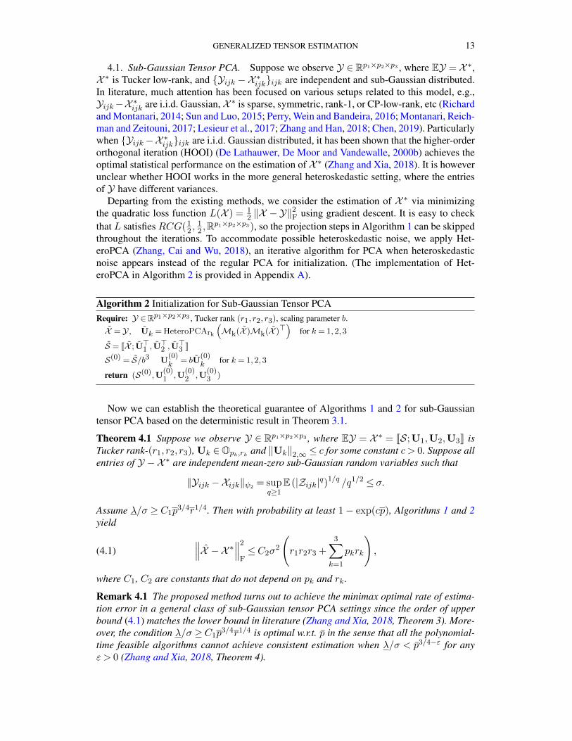
4.1. Sub-Gaussian Tensor PCA. Suppose we observe Y ∈ Rp1×p2×p3 , where EY = X ∗,X ∗ is Tucker low-rank, and Yijk −X ∗ijkijk are independent and sub-Gaussian distributed.In literature, much attention has been focused on various setups related to this model, e.g.,Yijk−X ∗ijk are i.i.d. Gaussian, X ∗ is sparse, symmetric, rank-1, or CP-low-rank, etc (Richardand Montanari, 2014; Sun and Luo, 2015; Perry, Wein and Bandeira, 2016; Montanari, Reich-man and Zeitouni, 2017; Lesieur et al., 2017; Zhang and Han, 2018; Chen, 2019). Particularlywhen Yijk−X ∗ijkijk are i.i.d. Gaussian distributed, it has been shown that the higher-orderorthogonal iteration (HOOI) (De Lathauwer, De Moor and Vandewalle, 2000b) achieves theoptimal statistical performance on the estimation of X ∗ (Zhang and Xia, 2018). It is howeverunclear whether HOOI works in the more general heteroskedastic setting, where the entriesof Y have different variances.

Departing from the existing methods, we consider the estimation of X ∗ via minimizingthe quadratic loss function L(X ) = 1

2 ‖X −Y‖2F using gradient descent. It is easy to check

that L satisfies RCG(12 ,

12 ,R

p1×p2×p3), so the projection steps in Algorithm 1 can be skippedthroughout the iterations. To accommodate possible heteroskedastic noise, we apply Het-eroPCA (Zhang, Cai and Wu, 2018), an iterative algorithm for PCA when heteroskedasticnoise appears instead of the regular PCA for initialization. (The implementation of Het-eroPCA in Algorithm 2 is provided in Appendix A).

Algorithm 2 Initialization for Sub-Gaussian Tensor PCARequire: Y ∈Rp1×p2×p3 , Tucker rank (r1, r2, r3), scaling parameter b.

X = Y, Uk = HeteroPCArk

(Mk(X )Mk(X )>

)for k = 1,2,3

S = JX ; U>1 , U>2 , U

>3 K

S(0) = S/b3 U(0)k = bU

(0)k for k = 1,2,3

return (S(0),U(0)1 ,U

(0)2 ,U

(0)3 )

Now we can establish the theoretical guarantee of Algorithms 1 and 2 for sub-Gaussiantensor PCA based on the deterministic result in Theorem 3.1.

Theorem 4.1 Suppose we observe Y ∈ Rp1×p2×p3 , where EY = X ∗ = JS;U1,U2,U3K isTucker rank-(r1, r2, r3), Uk ∈Opk,rk and ‖Uk‖2,∞ ≤ c for some constant c > 0. Suppose allentries of Y −X ∗ are independent mean-zero sub-Gaussian random variables such that

‖Yijk −Xijk‖ψ2= sup

q≥1E (|Zijk|q)1/q /q1/2 ≤ σ.

Assume λ/σ ≥ C1p3/4r1/4. Then with probability at least 1− exp(cp), Algorithms 1 and 2

yield

(4.1)∥∥∥X − X ∗∥∥∥2

F≤C2σ

2

(r1r2r3 +

3∑k=1

pkrk

),

where C1, C2 are constants that do not depend on pk and rk.

Remark 4.1 The proposed method turns out to achieve the minimax optimal rate of estima-tion error in a general class of sub-Gaussian tensor PCA settings since the order of upperbound (4.1) matches the lower bound in literature (Zhang and Xia, 2018, Theorem 3). More-over, the condition λ/σ ≥C1p

3/4r1/4 is optimal w.r.t. p in the sense that all the polynomial-time feasible algorithms cannot achieve consistent estimation when λ/σ < p3/4−ε for anyε > 0 (Zhang and Xia, 2018, Theorem 4).


4.2. Low-rank Tensor Regression. Motivated by applications of neuroimaging analysis(Zhou, Li and Zhu, 2013; Li and Zhang, 2017; Guhaniyogi, Qamar and Dunson, 2017),spatio-temporal forecasting (Bahadori, Yu and Liu, 2014), high-order interaction pursuit(Hao, Zhang and Cheng, 2019), longitudinal relational data analysis (Hoff, 2015), 3D imag-ing processing (Guo, Kotsia and Patras, 2012), among many others, we consider the low-ranktensor regression next. Suppose we observe a collection of data D = yi,Aini=1 that are as-sociated through the following equation:

(4.2) yi = 〈Ai,X ∗〉+ εi, εiiid∼ N(0, σ2), i= 1, . . . , n.

By exploiting the negative log-likelihood, it is natural to set L to be the squared loss function

L (X ;D) =

n∑i=1

(〈Ai,X〉− yi)2 .

To estimate X ∗, we first perform spectral method (Algorithm 3) to obtain initializer X (0) =

JS(0),U(0)1 ,U

(0)2 ,U

(0)3 K, then perform the gradient descent (Algorithm 1) without the projec-

tion steps to obtain the final estimator X . A key step of Algorithm 3 is HOSVD or HOOI,which are described in detail in Appendix A.

Algorithm 3 Initialization of Low-rank Tensor RegressionRequire: Ai, yi, i= 1, . . . , n, rank (r1, r2, r3), scaling parameter b.X = 1

n∑yiAi

(S, U1, U2, U3) = HOSVD(X)

or (S, U1, U2, U3) = HOOI(X)

U(0)k = bUk , for k = 1,2,3

S(0) = S/b3


(0)2 ,U

(0)3 )

For technical convenience, we assume the covariates Aini=1 are randomly designed thatall entries of Ai are i.i.d. drawn from sub-Gaussian distribution with mean 0 and variance 1.The following theorem gives an estimation error upper bound for Algorithms 1 and 3.

Theorem 4.2 Consider the low-rank tensor regression model (4.2). Suppose σ2 ≤C1 ‖X ∗‖2F, λ ≥ C2, and the sample size n ≥ C3 maxp3/2r, p · r2, r4 for constants

C1,C2,C3 > 0. Then with probability at least 1− exp−c(r1r2r3 +

∑3k=1 pkrk)

, the out-

put of Algorithms 1 and 3 satisfies∥∥∥X − X ∗∥∥∥2

F≤Cσ2

(r1r2r3 +

3∑k=1

pkrk

)/n,

where C1,C2,C3,C are constants depending only on κ and c > 0 is a universal constant.

Theorem 4.2 together with the lower bound in (Zhang et al., 2019, Theorem 5) shows thatthe proposed procedure achieves the minimax optimal rate of estimation error in the class ofall p1-by-p2-by-p3 tensors with rank-(r1, r2, r3) for tensor regression.

Remark 4.2 The assumption on the covariates Aini=1 in Theorem 4.2 ensures that X inAlgorithm 3 is an unbiased estimator of X ∗. Such a setting has been considered as a bench-mark setting in the high-dimensional statistical inference literature (see, e.g., Candes andPlan (2011); Chen, Raskutti and Yuan (2019); Javanmard et al. (2018)). When Aini=1 are


heteroskedastic, the spectral initialization may fail and an alternative idea is the followingunfolded nuclear norm minimization:

(4.3) X ′ = arg minX∈Rp1×p2×p3

3∑k=1

‖Mk(X )‖∗ , s.t. A(X ) = y.

(4.3) is equivalent to a semidefinite programming and can be solved by the interior-pointmethod (Gandy, Recht and Yamada, 2011).

Remark 4.3 There is a significant gap between the required sample size in Theorem 4.2(O(p3/2r)) and the possible sample size lower bound, i.e., the degree of freedom of all rank-rdimension-p tensor (O

(r3 + pr

)). The existing algorithms achieving the sample size lower

bound are often NP-hard to compute and thus intractable in practice. We also note that theexistence of a tractable algorithm for tensor completion that provably works with less thanp3/2−ε measurements would disapprove an open conjecture in theoretical computer scienceon strongly random 3-SAT (Barak and Moitra, 2016, Corollary 16). Since tensor completioncan be seen as a special case of tensor recovery, this suggests that it may be impossible tosubstantially improve the sample complexity required in Theorem 4.2 using a polynomial-time algorithm. Therefore, our procedure can be taken as the first computationally efficientalgorithm to achieve minimax optimal rate of convergence and exact recovery in the noiselesssetting as illustrated in Table 1.

4.3. Poisson Tensor PCA. Tensor data with count values commonly arise from variousscientific applications, such as the photon-limited imaging (Timmerman and Nowak, 1999;Willett and Nowak, 2007; Salmon et al., 2014; Yankovich et al., 2016), online click-throughdata analysis (Shan et al., 2016; Sun and Li, 2016), and metagenomic sequencing (Floreset al., 2014). In this section, we consider the Poisson tensor PCA model: assume we observeY ∈Np1×p2×p3 that satisfies

(4.4) Yijk ∼ Poisson(I exp(X ∗ijk)) independently,

where X ∗ is the low-rank tensor parameter and I > 0 is the intensity parameter. When X ∗ isentry-wise bounded (Assumption 4.1), one can set I as the average intensity of all entries ofY so that I essentially quantifies the signal-to-noise ratio. Rather than estimating I exp(X ∗),we focus on estimating X ∗, the key tensor that captures the salient geometry or structure ofthe data.

Then, the following negative log-likelihood is a natural choice of the loss function forestimating X ∗,

(4.5) L(X ) =

p1∑i=1

p2∑j=1

p3∑k=1

(−YijkXijk + I exp(Xijk)) .

Unfortunately, L(X ) defined in (4.5) satisfies RCG(α,β,C) only for a bounded set C sincethe Poisson likelihood function is not strongly convex and smooth in the unbounded domain.We thus introduce the following assumption on X ∗ to ensure that X ∗ is in a bounded set C.

Assumption 4.1 Suppose X ∗ = JS∗;U∗1,U∗2,U∗3K, where U∗k ∈Opk,rk is a pk-by-rk orthog-onal matrix for k = 1,2,3. There exist some constants µk3k=1,B such that ‖U∗k‖

22,∞ ≤

µkrkpk

for k = 1,2,3 and λ ≤ B√

Π3k=1pk

Π3k=1µkrk

where λ := maxk ‖Mk(S∗)‖. Here, ‖U∗k‖2,∞ =

maxi ‖(U∗k)i·‖2 is the largest row-wise `2 norm of U∗k.


Assumption 4.1 requires that the loading Uk satisfies the incoherence condition, i.e., the am-plitude of the tensor is “balanced” in all parts. Previously, the incoherence condition and itsvariations were commonly used in the matrix estimation literature (Candès and Recht, 2009;Ma and Ma, 2017) and Poisson-type inverse problems (e.g., Poisson sparse regression (Jiang,Raskutti and Willett, 2015, Assumption 2.1), Poisson matrix completion (Cao and Xie, 2015,Equation (10)), compositional matrix estimation (Cao, Zhang and Li, 2019, Equation (7)),Poisson auto-regressive models (Hall, Raskutti and Willett, 2016)). Assumption 4.1 also re-quires an upper bound on the spectral norm of each matricization of the core tensor S∗.Together with the incoherence condition on U∗k, this condition guarantees that X ∗ is entry-wise upper bounded by B. In fact, the entry-wise bounded assumption is also widely used inhigh-dimensional matrix/tensor generalized linear models since it guarantees the local strongconvexity and smoothness of the negative log-likelihood function (Ma and Ma, 2017; Wangand Li, 2018; Xu, Hu and Wang, 2019).

Next, we set (Ck3k=1,CS) as follows:

Ck =

Uk ∈Rpk×rk : ‖Uk‖2,∞ ≤ b

√µkrkpk

,

CS =

S ∈Rr1×r2×r3 : max

k‖Mk(S)‖ ≤ b−3B

√Π3k=1pk

Π3k=1µkrk

.

(4.6)

Specifically for the Poisson tensor PCA, we can prove that if Assumption 4.1 holds, the lossfunction (4.5) satisfiesRCG(α,β,Ck3k=1 ,CS) for constants α,β that only depend on I andB (see the proof of Theorem 4.3 for details). We can also show that the following Algorithm4 provides a sufficiently good initialization with high probability.

Algorithm 4 Initialization for Poisson Tensor PCARequire: Initialization observation tensor Y ∈ Np1×p2×p3 , Tucker rank (r1, r2, r3), scaling parameter b, in-

tensity parameter I .X = log

((Yjkl + 1

2 )/I)

(S, U1, U2, U3) = HOSVD(X)

or (S, U1, U2, U3) = HOOI(X)

U(0)k = bUk , for k = 1,2,3

S(0) = S/b3


(0)2 ,U

(0)3 )

Now we establish the estimation error upper bound for Algorithms 1 and 4.

Theorem 4.3 Suppose Assumption 4.1 holds and I > C1 maxp, λ−2∑3k=1(p−krk +

pkrk), where p−k := p1p2p3/pk. Then with probability at least 1 − c/(p1p2p3), the out-put of Algorithms 1 and 4 yields∥∥∥X − X ∗∥∥∥2

F≤C2I

−1

(r1r2r3 +

3∑k=1

pkrk

).

Here C1,C2 are constants that do not depend on pk or rk.

We further consider the following class of low-rank tensors Fp,r , where the restrictions inFp,r correspond to the conditions in Theorem 4.3:

Fp,r =

X = JS;U1,U2,U3K :Uk ∈Opk,rk , ‖Uk‖22,∞ ≤

µkrkpk

,

maxk‖Mk(S)‖ ≤B

√Π3

k=1pkΠ3

k=1µkrk

.(4.7)


With some technical conditions on tensor rank and the intensity parameter, we can developthe following lower bound in estimation error for Poisson PCA.

Theorem 4.4 (Lower Bound for Poisson tensor PCA) Assume r ≤ C1p1/2, r > C2 and

mink µk ≥ C3 for constants C1,C2,C3 > 1. Suppose one observes Y ∈ Rp1×p2×p3 , whereYjkl ∼ Poisson (I exp(Xjkl)) independently, X ∈ Fp,r , and I ≥ c0. There exists a uniformconstant c that does not depend on pk or rk, such that

infX

supX∈Fp,r

E∥∥∥X − X∥∥∥2

F≥ cI−1

(r1r2r3 +

3∑k=1

pkrk

).

Theorems 4.3 and 4.4 together yield the optimal rate of estimation error for Poisson tensorPCA problem over the class of Fp,r:

infX

supX∈Fp,r

E∥∥∥X − X∥∥∥2

F I−1

(r1r2r3 +

3∑k=1

pkrk

).

4.4. Binomial Tensor PCA. The binomial tensor data commonly arise in the analysis ofproportion when raw counts are available. For example, in the Human Mortality Database(Wilmoth and Shkolnikov, 2006), the number of deaths and the total number of populationare summarized into a three-way tensor, where the x-, y-, z-coordinates are counties, ages,and years, respectively. Given the sufficiently large number of population in each country,one can generally assume that each entry of this data tensor satisfies the binomial distributionindependently.

Suppose we observe a count tensor Y ∈ Np1×p2×p3 and a total population tensor N ∈Np1×p2×p3 such that Yjkl ∼ Binomial(Njkl,P∗jkl) independently. Here, P∗ ∈ [0,1]p1×p2×p3

is a probability tensor linked to an underlying latent parameter X ∗ ∈ Rp1×p2×p3 throughP∗jkl = s(X ∗jkl), where s(x) = 1/(1 + e−x) is the sigmoid function. Our goal is to estimateX ∗. To this end, we consider to minimize the following loss function:

L(X ) =−∑jkl

(PjklXjkl + log (1− σ(Xjkl))

),

where Pjkl := Yjkl/Njkl.We assumeX ∗ satisfies Assumption 4.1 for the same reasons as in Poisson tensor PCA. We

propose to estimate P∗ by applying Algorithm 5 (initialization) and Algorithm 1 (projectedgradient descent) with the following constraint sets:

Ck =

Uk ∈Rpk×rk : ‖Uk‖2,∞ ≤ b

√µkrkpk

,

CS =

S ∈Rr1×r2×r3 : max

k‖Mk(S)‖ ≤ b−3B

√Π3k=1pk

Π3k=1µkrk

.

We have the following theoretical guarantee for the estimator obtained by Algorithms 1and 5 in binomial tensor PCA.

Theorem 4.5 (Upper Bound for Binomial Tensor PCA) Suppose Assumption 4.1 is satis-fied and N = minjklNjkl satisfies N ≥ C1 max

p,λ−2∑

k (p−krk + pkrk)

. Then withprobability at least 1 − c/(p1p2p3), we have the following estimation upper bound for theoutput of Algorithms 1 and 5:∥∥∥X − X ∗∥∥∥2

F≤C2N

−1

(r1r2r3 +

3∑k=1

pkrk

).


Algorithm 5 Initialization for Binomial Tensor PCARequire: Y,N ∈Np1×p2×p3 , Tucker rank (r1, r2, r3), scaling parameter b

Xjkl = log

(Yjkl+1/2

Njkl−Yjkl+1/2

), ∀j, k, l

(S, U1, U2, U3) = HOSVD(X)

or (S, U1, U2, U3) = HOOI(X)

U(0)k = bUk , for k = 1,2,3

S(0) = S/b3


(0)2 ,U

(0)3 )

Here, C1,C2 are some absolute constants that do not depend on pk or rk.

Remark 4.4 We assume N ≥ C1 maxp,λ−2∑

k (p−krk + pkrk)

in Theorem 4.5 as atechnical condition to prove the estimation error upper bound of X . N here essentially char-acterizes the signal-noise ratio of the binomial tensor PCA problem.

Let Fp,r be the class of low-rank tensors defined in (4.7). We can prove the following lowerbound result, which establishes the minimax optimality of the proposed procedure over theclass of Fp,r in binomial tensor PCA.

Theorem 4.6 (Lower Bound for Binomial Tensor PCA) Denote N = minjklNjkl. As-sume r ≤C1p

1/2, r > C2 and mink µk ≥C3 for some constants C1,C2,C3 > 1. Suppose oneobserves Y ∈ Np1×p2×p3 , where Yjkl ∼ Binomial (Njkl, σ(Xjkl)) independently, X ∗ ∈ Fp,r ,and maxjklNjkl ≤ CminjklNjkl. There exists constant c that does not depend on pk or rk,such that

infX

supX∈Fp,r

∥∥∥X − X∥∥∥2

F≥ cN−1

(r1r2r3 +

3∑k=1

pkrk

).

5. Rank Selection. The tensor rank (r1, r2, r3) is required as an input to Algorithm 1and plays a crucial role in the proposed non-convex optimization framework. While variousempirical methods have been proposed for rank selection in specific applications of low-ranktensor estimation (e.g., Yokota, Lee and Cichocki (2016)), there is a paucity of theoreticalguarantees in the literature. In this section, we provide a rank estimation procedure withprovable guarantees. Recall that in each application in Section 4, we first specify the initial-ization X (0) = JS(0);U

(0)1 ,U

(0)2 ,U

(0)3 K based on a spectral algorithm on some preliminary

tensor X (see their definitions in Algorithms 2-5). Since X reflects the target tensor X ∗ andσs(Mk(X ∗)) = 0 for s ≥ rk + 1, we consider the following rank selection method by ex-ploiting the singular values of X :

(5.1) rk = maxr : σr

(Mk(X )

)≥ tk

, k = 1,2,3.

Here, tk > 0 is the thresholding level whose value depends on specific problem settings.Next, we specifically consider the sub-Gaussian tensor PCA and tensor regression.

Proposition 5.1 Suppose rank(X ∗) = (r1, r2, r3), rk = o(pk), pk = o(p−k). Define rk as(5.1) and

(5.2) δk := Medianσ1(Mk(X )), . . . , σpk

(Mk(X )

).

(a) In sub-Gaussian tensor PCA (Section 4.1), we set X = Y, tk = 1.5δk. Suppose λ≥Cpσ.Then, we have rk = rk,∀k ∈ [d] with probability at least 1−Ce−cp.


(b) In low-rank tensor regression (Section 4.2), we set X = 1n

∑ni=1 yiAi, tk = 1.5δk. Sup-

pose n≥ Cκp2r3/2 log r and λ≥ C pσ√n

. Then, rk = rk,∀k ∈ [d] with probability at least1−Ce−cp.

In practice, we can also apply a simple criterion of the cumulative percentage of totalvariation (Jolliffe, 1986, Chapter 6.1.1) originating from principle component analysis:

(5.3) rk = arg min

r :

r∑i=1

σ2i (Mk(X ))

/ pk∑i=1

σ2i (Mk(X ))≥ ρ

Here, ρ ∈ (0,1) is some empirical thresholding level. We will illustrate this principle on realdata analysis in Section 7.2. Under the general deterministic setting, the accurate (or optimal)estimation of tensor rank may be much more challenging and we leave it as future work.

6. Extensions to General Order-d Tensors. While our previous sections mainly focuson order-3 tensor estimation, our results can be generalized to the order-d low-rank tensorestimation with the key ideas outline in this section. First, the constraint set C, RCG conditionand noise quantity ξ can be defined similarly by replacing the order-3 tensor with the generallow-rank order-d tensors; second, the local convergence analysis can be similarly conductedas Theorem 3.1. Define

E(t) := minRk∈Opk,rkk=1,...,d

d∑

k=1


∥∥∥2

F+∥∥∥S(t) − JS∗;R>1 , . . . ,R>d K

∥∥∥2

F

.

We can build the equivalence between E(t) and∥∥∥X (t) −X ∗∥∥∥2

F+a

2

d∑k=1

∥∥∥U(t)>k U

(t)k − b

2Irk

∥∥∥2

F

by setting b λ1/(d+1)and a λ. Then, we can establish the following theoretical guarantee

under a good initialization:

Theorem 6.1 (Informal) Suppose L satisfies RCG(α,β,C) and assume κ,α,β are con-stants. Assume X ∗ = JS∗;U∗1, . . . ,U∗dK and the initialization X (0) = JS(0);U

(0)1 , . . . ,U

(0)d K

satisfy

U∗>k U∗k = U(0)>k U

(0)k = b2Irk , U∗k,U

(0)k ∈ Ck, k = 1, . . . , d; S∗,S(k) ∈ CS .(6.1)

Suppose the initialization error satisfies∥∥X (0) −X ∗

∥∥≤ cdλ2 and the signal-noise-ratio sat-isfies λ2 ≥Cdξ2. Then, by taking step size η ≤ cdb−2d, the output of Algorithm 3.1 satisfies∥∥∥X (t) −X ∗

∥∥∥2

F≤C ′d

(ξ2 +

(1− c′dη

)t ∥∥∥X (0) −X ∗∥∥∥2

F

).

Here, Cd, cd,C ′d, c′d are constants only depending on d.

It is worth mentioning that Theorem 6.1 applies to low-rank matrix estimation (i.e. d = 2):suppose X∗ = U∗1S

∗U∗>2 and X(0) = U(0)1 S(0)U

(0)>2 for Uk,U

(0)k ∈ Rpk×r , S∗,S(0) ∈

Rr×r , we have ∥∥∥X(t) −X∗∥∥∥2

F≤C

(ξ2 + (1− cη)t

∥∥∥X(0) −X∗∥∥∥2

F

).


Application SNR condition Estimation error Lower bound

sub-Gaussian tensor-PCA λ/σ & pd/4r1/(d+1) σ2(pr+ rd

)σ2(pr+ rd

)Tensor regression n& pd/2r n−1σ2

(pr+ rd

)n−1σ2

(pr+ rd

)Poisson tensor-PCA

√Iλ& p(d−1)/2r1/2 I−1

(pr+ rd

)I−1

(pr+ rd

)Binomial tensor-PCA

√Nλ& p(d−1)/2r1/2 N−1

(pr+ rd

)N−1

(pr+ rd

)TABLE 2

Minimax optimal estimation error bounds for order-d low-rank tensor estimation in specific applications(d≥ 2). Here, for simplicity, r1 = r2 = r3 = r, p1 = p2 = p3 = p and r ≤ p1/2.

While this framework is more complicated than necessary since one can always decomposea low-rank matrix as the product of two factor matrices X = U1U

>2 without explicitly intro-

ducing the “core matrix” S ∈Rr×r (see our previous discussions in Section 3.3).Based on Theorem 6.1, we can further extend the minimax optimal bounds for the pro-

posed procedure in each application of Section 4, i.e., Theorems 4.1–4.6 to high-order sce-narios. We summarize the results to Table 2.

7. Numerical Studies.

7.1. Synthetic Data Analysis. In this section, we investigate the numerical performanceof the proposed methods on the problems discussed in Section 4 with simulated data. Weassume the true rank (r1, r2, r3) is known to us and the algorithm only involves two tuningparameters: a and b. According to Theorem 3.1, a proper choice of a and b primarily dependson the unknown value λ. In practice, we propose to use the initial estimate X (0) as an ap-proximation of X ∗, use λ(0) = maxk

∥∥Mk(X (0))∥∥ as a plug-in estimate of λ, then choose

a= λ(0), b= (λ

(0))1/4. We consider the following root mean squared error (RMSE) to assess

the estimation accuracy in all settings:

(7.1) Loss(X ,X ∗) = (p1p2p3)−1/2‖X −X ∗‖F.

Average loss over 100 repetitions are reported in following different scenarios.

Tensor Regression. We investigate the numerical performance of the proposed procedurein low-rank tensor regression discussed in Section 4.2. For all simulation settings, we firstgenerate an r1-by-r2-by-r3 core tensor S with i.i.d. standard Gaussian entries and rescale itas S = S · λ/min3

k=1 σr(Mk(S)

). Here, λ quantifies the signal level and will be specified

later. Then we generate Uk uniformly at random from the Stiefel manifold Opk,rk and calcu-late the true parameter as X ∗ = JS;U1,U2,U3K. The rescaling procedure here ensures thatmink σrk (Mk(X ∗)) ≥ λ. Now, we draw a random sample based on the regression model(4.2).

We aim to compare the proposed method (Algorithms 1 and 3) with the initializationestimator (Algorithm 3 solely), Tucker-Regression method2, and MLE. Since the MLE cor-responds to the global minimum of the rank-constrained optimization (2.2) and is often com-putationally intractable, we instead consider a warm-start gradient descent estimator, i.e.,performing Algorithm 1 starting from the true parameter X ∗. We expect that the output ofthis procedure can well approximate MLE. We implement all four procedures under twosettings: (a) p1 = p2 = p3 = p = 30, r1 = r2 = r3 = r = 5, λ = 2, σ = 1, n varies from300 to 1000; and (b) p varies from 20 to 50, r = 3, λ = 2, σ = 1, n = 1.2p3/2r. The results

2The implementation is based on (Zhou, Li and Zhu, 2013; Zhou, 2017).


FIG 1. Average estimation errors in low-rank tensor regression. The MLE (oracle) is approximated by runninggradient descent with the initialization chosen at X ∗, which would not be useable in practice. Here, r = 3, λ= 2,σ = 1. Left panel: p= 30, n ∈ [300,1000]. Right panel: p ∈ [25,50], n= 1.2p3/2r.

are collected in Figure 1. We see from the left panel that for small sample size (n ≤ 600),the proposed gradient descent method significantly outperforms the Tucker-Regression andinitialization estimator while has larger estimation errors than MLE. When the sample sizeincreases (n ≥ 700), the performance of the proposed gradient descent and Tucker regres-sion algorithms tend to be as good as MLE. Compared to the initialization, gradient descentachieves a great improvement on the estimation accuracy. The right panel of Figure 1 showsthat the gradient descent performs as good as the warm-start gradient descent asymptoticallyand is significantly better than the initialization and Tucker-Regression estimators.

Poisson Tensor PCA. Next, we study the numerical performance of the proposed procedureon Poisson tensor PCA. As mentioned earlier in Section 4.3, we found that the projectionsteps in Algorithm 1 are not essential to the numerical performance, thus we apply Algorithm1 without the projection steps there in all numerical experiments for Poisson tensor PCA.

For each experiment, we first generate a random core tensor S ∈ Rr1×r2×r3 with i.i.d.standard normal entries and random orthogonal matrices Uk uniformly on Stiefel manifoldOpk×rk . Then we calculate X = S ×1 U1×2 U2×3 U3 and rescale it as X ∗ = X ·B/

∥∥X∥∥∞to ensure that each entry of X ∗ is bounded by B. Now, we generate a count tensorY ∈ Np1×p2×p3 : Yjkl ∼ Poisson(I exp(X ∗jkl)) independently, and aim to estimate the low-rank tensor X ∗ based on Y . In addition to the proposed method, we also consider the base-line methods of Poisson-HOSVD and Poisson-HOOI that perform HOSVD and HOOI onlog ((Y + 1/2)/I) (i.e., Algorithm 4).

First, we fix p = 50, r = 5, vary the intensity value I , and study the effect of I to thenumerical performance. As we can see from Figure 2, for low intensity, the gradient methodis significantly better than two baselines (left panel); for high intensity, three methods arecomparable while the Poisson gradient descent is the best (right panel). Next, we study theirperformance for different tensor dimensions and ranks. In the left panel of Figure 3, we setr = 5 and vary p from 30 to 100; in the right panel of Figure 3, we fix p= 50 and vary r from5 to 15. As one can see, our method significantly outperforms the baselines in all settings.All these simulation results illustrate the benefits of applying gradient descent on the Poissonlikelihood function.

Binomial Tensor PCA. We generate X ∗ in the same way as the Poisson tensor PCA settings.Suppose we observe Y ∈Np1×p2×p3 generated from

Yjkl ∼ Binomial(Njkl, s(X ∗jkl)

), independently.


FIG 2. Average estimation error of Poisson tensor PCA. Here p= 50, r = 5, B = 2. Left panel: intensity param-eter I ∈ [.5,2]. Right panel: I ∈ [2,20].

FIG 3. Average estimation error of Poisson tensor PCA with different dimensions and ranks. Here, B = 2, I = 1.Left panel: r = 5, p ∈ [30,300]. Right panel: p= 50, r ∈ [5,15].

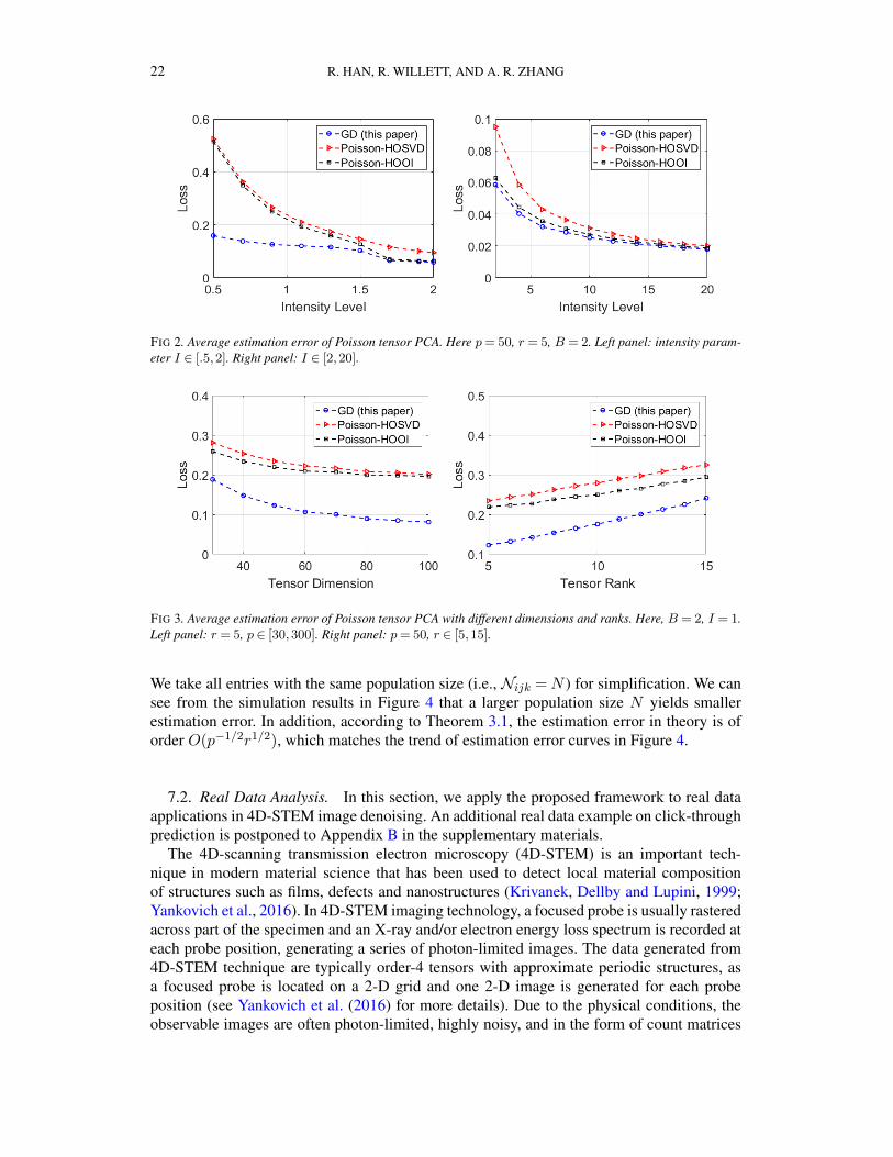
We take all entries with the same population size (i.e., Nijk =N ) for simplification. We cansee from the simulation results in Figure 4 that a larger population size N yields smallerestimation error. In addition, according to Theorem 3.1, the estimation error in theory is oforder O(p−1/2r1/2), which matches the trend of estimation error curves in Figure 4.

7.2. Real Data Analysis. In this section, we apply the proposed framework to real dataapplications in 4D-STEM image denoising. An additional real data example on click-throughprediction is postponed to Appendix B in the supplementary materials.

The 4D-scanning transmission electron microscopy (4D-STEM) is an important tech-nique in modern material science that has been used to detect local material compositionof structures such as films, defects and nanostructures (Krivanek, Dellby and Lupini, 1999;Yankovich et al., 2016). In 4D-STEM imaging technology, a focused probe is usually rasteredacross part of the specimen and an X-ray and/or electron energy loss spectrum is recorded ateach probe position, generating a series of photon-limited images. The data generated from4D-STEM technique are typically order-4 tensors with approximate periodic structures, asa focused probe is located on a 2-D grid and one 2-D image is generated for each probeposition (see Yankovich et al. (2016) for more details). Due to the physical conditions, theobservable images are often photon-limited, highly noisy, and in the form of count matrices


FIG 4. Average estimation error of binomial tensor PCA. Here, B = 2. Left panel: r = 5, p ∈ [30,100]. Rightpanel: p= 50, r ∈ [5 : 15].

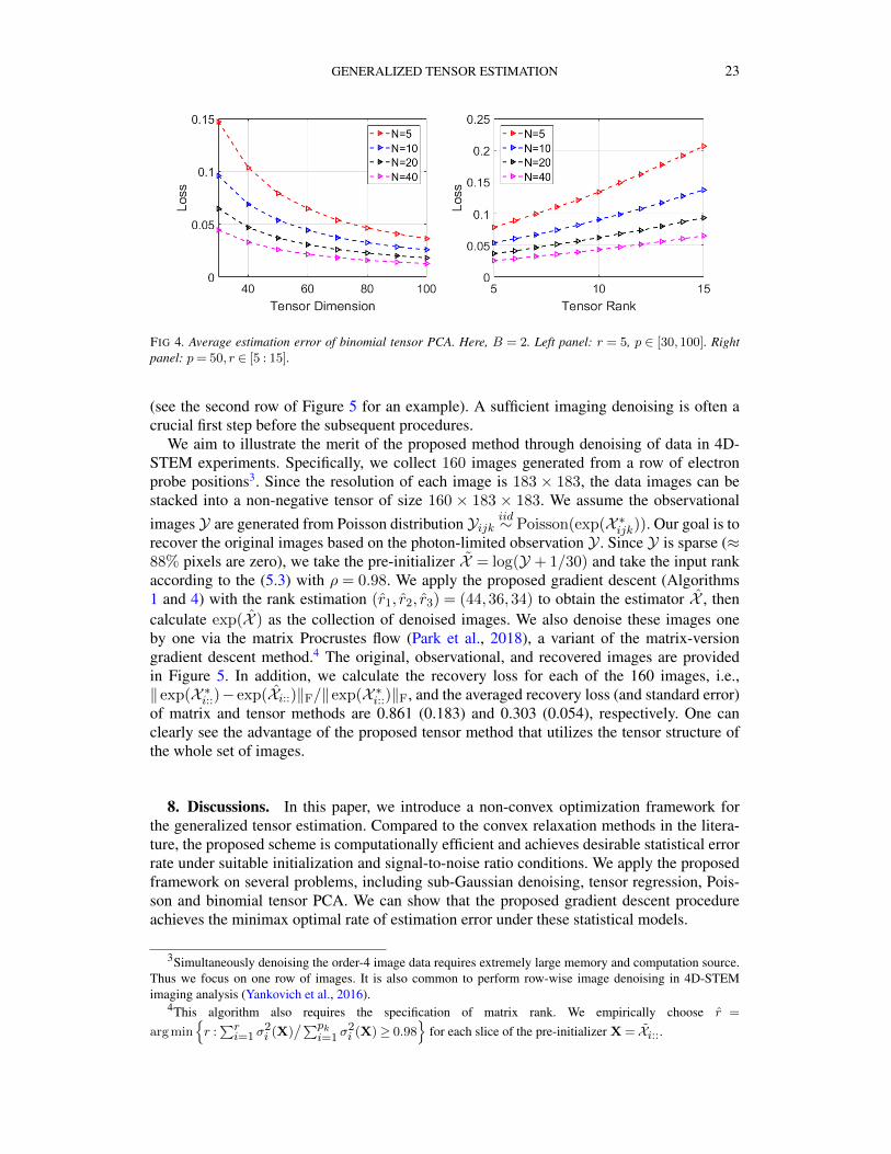
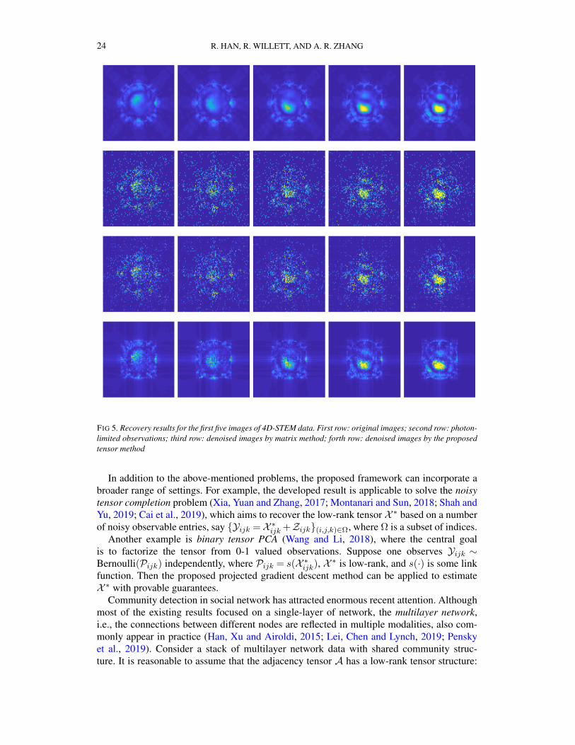
(see the second row of Figure 5 for an example). A sufficient imaging denoising is often acrucial first step before the subsequent procedures.

We aim to illustrate the merit of the proposed method through denoising of data in 4D-STEM experiments. Specifically, we collect 160 images generated from a row of electronprobe positions3. Since the resolution of each image is 183 × 183, the data images can bestacked into a non-negative tensor of size 160 × 183 × 183. We assume the observationalimages Y are generated from Poisson distribution Yijk

iid∼ Poisson(exp(X ∗ijk)). Our goal is torecover the original images based on the photon-limited observation Y . Since Y is sparse (≈88% pixels are zero), we take the pre-initializer X = log(Y + 1/30) and take the input rankaccording to the (5.3) with ρ = 0.98. We apply the proposed gradient descent (Algorithms1 and 4) with the rank estimation (r1, r2, r3) = (44,36,34) to obtain the estimator X , thencalculate exp(X ) as the collection of denoised images. We also denoise these images oneby one via the matrix Procrustes flow (Park et al., 2018), a variant of the matrix-versiongradient descent method.4 The original, observational, and recovered images are providedin Figure 5. In addition, we calculate the recovery loss for each of the 160 images, i.e.,‖ exp(X ∗i::)− exp(Xi::)‖F/‖ exp(X ∗i::)‖F, and the averaged recovery loss (and standard error)of matrix and tensor methods are 0.861 (0.183) and 0.303 (0.054), respectively. One canclearly see the advantage of the proposed tensor method that utilizes the tensor structure ofthe whole set of images.

8. Discussions. In this paper, we introduce a non-convex optimization framework forthe generalized tensor estimation. Compared to the convex relaxation methods in the litera-ture, the proposed scheme is computationally efficient and achieves desirable statistical errorrate under suitable initialization and signal-to-noise ratio conditions. We apply the proposedframework on several problems, including sub-Gaussian denoising, tensor regression, Pois-son and binomial tensor PCA. We can show that the proposed gradient descent procedureachieves the minimax optimal rate of estimation error under these statistical models.

3Simultaneously denoising the order-4 image data requires extremely large memory and computation source.Thus we focus on one row of images. It is also common to perform row-wise image denoising in 4D-STEMimaging analysis (Yankovich et al., 2016).

4This algorithm also requires the specification of matrix rank. We empirically choose r =

arg minr :∑ri=1 σ

2i (X)

/∑pki=1 σ

2i (X)≥ 0.98

for each slice of the pre-initializer X = Xi::.


FIG 5. Recovery results for the first five images of 4D-STEM data. First row: original images; second row: photon-limited observations; third row: denoised images by matrix method; forth row: denoised images by the proposedtensor method

In addition to the above-mentioned problems, the proposed framework can incorporate abroader range of settings. For example, the developed result is applicable to solve the noisytensor completion problem (Xia, Yuan and Zhang, 2017; Montanari and Sun, 2018; Shah andYu, 2019; Cai et al., 2019), which aims to recover the low-rank tensor X ∗ based on a numberof noisy observable entries, say Yijk =X ∗ijk +Zijk(i,j,k)∈Ω, where Ω is a subset of indices.

Another example is binary tensor PCA (Wang and Li, 2018), where the central goalis to factorize the tensor from 0-1 valued observations. Suppose one observes Yijk ∼Bernoulli(Pijk) independently, where Pijk = s(X ∗ijk), X ∗ is low-rank, and s(·) is some linkfunction. Then the proposed projected gradient descent method can be applied to estimateX ∗ with provable guarantees.

Community detection in social network has attracted enormous recent attention. Althoughmost of the existing results focused on a single-layer of network, the multilayer network,i.e., the connections between different nodes are reflected in multiple modalities, also com-monly appear in practice (Han, Xu and Airoldi, 2015; Lei, Chen and Lynch, 2019; Penskyet al., 2019). Consider a stack of multilayer network data with shared community struc-ture. It is reasonable to assume that the adjacency tensor A has a low-rank tensor structure:


A ∼ Bernoulli(X ∗) independently, where X ∗ = JS∗,Z∗,Z∗,T∗K, Z∗ is the latent space ofnodes features (or the indicator matrix for the community that each node belongs to), andT∗ models the trend along the time. Then the community detection for multilayer networksessentially becomes the generalized tensor estimation problem.

In addition to the standard linear regression model discussed in Section 4.2, the proposedframework can be applied to a range of generalized tensor regression problems. Recall thatthe classical generalized linear model focuses on an exponential family, where the response yisatisfies the following density or probability mass function (Nelder and Wedderburn, 1972),

(8.1) p(yi|θi, φ) = exp

yθi − b(θi)a(φ)

+ c(y,φ)

.

Here, a, b, c are prespecified functions determined by the problem; θi and φ > 0 are naturaland dispersion parameters, respectively. For the generalized tensor regression, it is natural torelate the tensor covariate and response (Zhou, Li and Zhu, 2013) via

(8.2) µi = E(yi|X ∗) g(µi) = 〈Ai,X ∗〉,

where g(·) is a link function. To estimate X ∗, we can apply the proposed Algorithm 3 on thenegative log-likelihood function

n∑i=1

yiθi − b(θi)a(φ)

+

n∑i=1

c(yi, φ),

where θi is determined by (8.1) and (8.2).Some other possible applications of the proposed framework include the high-order inter-

action pursuit (Hao, Zhang and Cheng, 2019), generalized regression among multiple modes(Xu, Hu and Wang, 2019), mixed-data-type tensor data analysis (Baker, Tang and Allen,2019), etc. In all these problems, by exploring the log-likelihood of data and the domain Cthat satisfies RCG condition, the proposed projected gradient descent can be applied and thetheoretical guarantees can be developed based on the proposed framework.

Acknowledgement. The authors thank Paul Voyles and Chenyu Zhang for providing the4D-STEM dataset and for helpful discussions. The research of R. H. and A. R. Z. was sup-ported in part by NSF DMS-1811868, NSF CAREER-1944904, and NIH R01-GM131399.The research of R. W. was supported in part by AFOSR FA9550-18-1-0166, DOE DE-AC02-06CH11357, NSF OAC-1934637, and NSF DMS-2023109. The research of R. H.was also supported in part by a RAship from Institute for Mathematics of Data Science atUW-Madison.

REFERENCES

AHMED, A., RECHT, B. and ROMBERG, J. (2013). Blind deconvolution using convex programming. IEEE Trans-actions on Information Theory 60 1711–1732.

ANANDKUMAR, A., HSU, D. and KAKADE, S. M. (2012). A method of moments for mixture models and hiddenMarkov models. In Conference on Learning Theory 33–1.

ANANDKUMAR, A., GE, R., HSU, D., KAKADE, S. M. and TELGARSKY, M. (2014). Tensor decompositionsfor learning latent variable models. The Journal of Machine Learning Research 15 2773–2832.

ARROYO, J., ATHREYA, A., CAPE, J., CHEN, G., PRIEBE, C. E. and VOGELSTEIN, J. T. (2019). Inference formultiple heterogeneous networks with a common invariant subspace. arXiv preprint arXiv:1906.10026.

BAHADORI, M. T., YU, Q. R. and LIU, Y. (2014). Fast multivariate spatio-temporal analysis via low rank tensorlearning. In Advances in neural information processing systems 3491–3499.

BAKER, Y., TANG, T. M. and ALLEN, G. I. (2019). Feature Selection for Data Integration with Mixed Multi-view Data. arXiv preprint arXiv:1903.11232.


BARAK, B. and MOITRA, A. (2016). Noisy tensor completion via the sum-of-squares hierarchy. In Conferenceon Learning Theory 417–445.

BI, X., QU, A. and SHEN, X. (2018). Multilayer tensor factorization with applications to recommender systems.The Annals of Statistics 46 3308–3333.

BIRGÉ, L. (2001). An alternative point of view on Lepski’s method. Lecture Notes-Monograph Series 113–133.BOUCHERON, S., LUGOSI, G. and MASSART, P. (2013). Concentration inequalities: A nonasymptotic theory of

independence. Oxford university press.CAI, T. T., LI, X. and MA, Z. (2016). Optimal rates of convergence for noisy sparse phase retrieval via thresh-

olded Wirtinger flow. The Annals of Statistics 44 2221–2251.CAI, T. T. and ZHANG, A. (2018). Rate-optimal perturbation bounds for singular subspaces with applications to

high-dimensional statistics. The Annals of Statistics 46 60–89.CAI, C., LI, G., POOR, H. V. and CHEN, Y. (2019). Nonconvex Low-Rank Tensor Completion from Noisy Data.

In Advances in Neural Information Processing Systems 1861–1872.CANDES, E. J., LI, X. and SOLTANOLKOTABI, M. (2015). Phase retrieval via Wirtinger flow: Theory and algo-

rithms. IEEE Transactions on Information Theory 61 1985–2007.CANDES, E. J. and PLAN, Y. (2010). Matrix completion with noise. Proceedings of the IEEE 98 925–936.CANDES, E. J. and PLAN, Y. (2011). Tight oracle inequalities for low-rank matrix recovery from a minimal

number of noisy random measurements. IEEE Transactions on Information Theory 57 2342–2359.CANDÈS, E. J. and RECHT, B. (2009). Exact matrix completion via convex optimization. Foundations of Com-

putational mathematics 9 717.CAO, Y. and XIE, Y. (2015). Poisson matrix recovery and completion. IEEE Transactions on Signal Processing

64 1609–1620.CAO, Y., ZHANG, A. and LI, H. (2019). Multi-sample estimation of bacterial composition matrix in metage-

nomics data. Biometrika.CHEN, W.-K. (2019). Phase transition in the spiked random tensor with rademacher prior. The Annals of Statistics

47 2734–2756.CHEN, Y. and CANDES, E. (2015). Solving random quadratic systems of equations is nearly as easy as solving

linear systems. In Advances in Neural Information Processing Systems 739–747.CHEN, Y. and CHI, Y. (2018). Harnessing structures in big data via guaranteed low-rank matrix estimation. arXiv

preprint arXiv:1802.08397.CHEN, H., RASKUTTI, G. and YUAN, M. (2019). Non-convex projected gradient descent for generalized low-

rank tensor regression. The Journal of Machine Learning Research 20 172–208.CHI, E. C. and KOLDA, T. G. (2012). On tensors, sparsity, and nonnegative factorizations. SIAM Journal on

Matrix Analysis and Applications 33 1272–1299.CHI, Y., LU, Y. M. and CHEN, Y. (2019). Nonconvex optimization meets low-rank matrix factorization: An

overview. IEEE Transactions on Signal Processing 67 5239–5269.CHI, E. C., GAINES, B. R., SUN, W. W., ZHOU, H. and YANG, J. (2018). Provable Convex Co-clustering of

Tensors. arXiv:1803.06518 [stat.ME].DE LATHAUWER, L., DE MOOR, B. and VANDEWALLE, J. (2000a). A multilinear singular value decomposition.

SIAM journal on Matrix Analysis and Applications 21 1253–1278.DE LATHAUWER, L., DE MOOR, B. and VANDEWALLE, J. (2000b). On the best rank-1 and rank-(r 1, r 2,..., rn)

approximation of higher-order tensors. SIAM Journal on Matrix Analysis and Applications 21 1324–1342.FAN, J., GONG, W. and ZHU, Z. (2019). Generalized high-dimensional trace regression via nuclear norm regu-

larization. Journal of Econometrics.FAUST, K., SATHIRAPONGSASUTI, J. F., IZARD, J., SEGATA, N., GEVERS, D., RAES, J. and HUTTEN-

HOWER, C. (2012). Microbial co-occurrence relationships in the human microbiome. PLoS computationalbiology 8 e1002606.

FAZEL, M. (2002). Matrix rank minimization with applications.FLORES, G. E., CAPORASO, J. G., HENLEY, J. B., RIDEOUT, J. R., DOMOGALA, D., CHASE, J., LEFF, J. W.,

VÁZQUEZ-BAEZA, Y., GONZALEZ, A., KNIGHT, R. et al. (2014). Temporal variability is a personalizedfeature of the human microbiome. Genome biology 15 531.

FRIEDLAND, S. and LIM, L.-H. (2018). Nuclear norm of higher-order tensors. Mathematics of Computation 871255–1281.

GANDY, S., RECHT, B. and YAMADA, I. (2011). Tensor completion and low-n-rank tensor recovery via convexoptimization. Inverse Problems 27 025010.

GUHANIYOGI, R., QAMAR, S. and DUNSON, D. B. (2017). Bayesian tensor regression. The Journal of MachineLearning Research 18 2733–2763.

GUO, W., KOTSIA, I. and PATRAS, I. (2012). Tensor learning for regression. IEEE Transactions on Image Pro-cessing 21 816–827.


HALL, E. C., RASKUTTI, G. and WILLETT, R. (2016). Inference of high-dimensional autoregressive generalizedlinear models. arXiv preprint arXiv:1605.02693.

HAN, Q., XU, K. and AIROLDI, E. (2015). Consistent estimation of dynamic and multi-layer block models. InInternational Conference on Machine Learning 1511–1520.

HAO, B., ZHANG, A. and CHENG, G. (2019). Sparse and Low-rank Tensor Estimation via Cubic Sketchings.The Annals of Statistics revision under review.

HENRIQUES, R. and MADEIRA, S. C. (2019). Triclustering algorithms for three-dimensional data analysis: Acomprehensive survey. ACM Computing Surveys (CSUR) 51 95.

HILLAR, C. J. and LIM, L.-H. (2013). Most tensor problems are NP-hard. Journal of the ACM (JACM) 60 45.HOFF, P. D. (2015). Multilinear tensor regression for longitudinal relational data. The annals of applied statistics

9 1169.HONG, D., KOLDA, T. G. and DUERSCH, J. A. (2018). Generalized canonical polyadic tensor decomposition.

arXiv preprint arXiv:1808.07452.HOPKINS, S. B., SHI, J. and STEURER, D. (2015). Tensor principal component analysis via sum-of-square

proofs. In Proceedings of The 28th Conference on Learning Theory, COLT 3–6.JAVANMARD, A., MONTANARI, A. et al. (2018). Debiasing the lasso: Optimal sample size for gaussian designs.

The Annals of Statistics 46 2593–2622.JIANG, X., RASKUTTI, G. and WILLETT, R. (2015). Minimax optimal rates for Poisson inverse problems with

physical constraints. IEEE Transactions on Information Theory 61 4458–4474.JOHNDROW, J. E., BHATTACHARYA, A. and DUNSON, D. B. (2017). Tensor decompositions and sparse log-

linear models. The Annals of Statistics 45 1–38.JOLLIFFE, I. T. (1986). Principal components in regression analysis. In Principal component analysis 129–155.

Springer.KESHAVAN, R. H., MONTANARI, A. and OH, S. (2010). Matrix completion from noisy entries. Journal of

Machine Learning Research 11 2057–2078.KOLDA, T. G. and BADER, B. W. (2009). Tensor decompositions and applications. SIAM review 51 455–500.KOLTCHINSKII, V., LOUNICI, K. and TSYBAKOV, A. B. (2011). Nuclear-norm penalization and optimal rates

for noisy low-rank matrix completion. The Annals of Statistics 39 2302–2329.KRIVANEK, O., DELLBY, N. and LUPINI, A. (1999). Towards sub-A electron beams. Ultramicroscopy 78 1–11.KROONENBERG, P. M. (2008). Applied multiway data analysis 702. John Wiley & Sons.LEI, J., CHEN, K. and LYNCH, B. (2019). Consistent community detection in multi-layer network data.

Biometrika.LESIEUR, T., MIOLANE, L., LELARGE, M., KRZAKALA, F. and ZDEBOROVÁ, L. (2017). Statistical and compu-

tational phase transitions in spiked tensor estimation. In 2017 IEEE International Symposium on InformationTheory (ISIT) 511–515. IEEE.

LI, N. and LI, B. (2010). Tensor completion for on-board compression of hyperspectral images. In 2010 IEEEInternational Conference on Image Processing 517–520. IEEE.

LI, L. and ZHANG, X. (2017). Parsimonious tensor response regression. Journal of the American StatisticalAssociation 1–16.

LI, X., XU, D., ZHOU, H. and LI, L. (2018). Tucker tensor regression and neuroimaging analysis. Statistics inBiosciences 10 520–545.

LIU, J., MUSIALSKI, P., WONKA, P. and YE, J. (2013). Tensor completion for estimating missing values invisual data. IEEE Transactions on Pattern Analysis and Machine Intelligence 35 208–220.

LUBICH, C., ROHWEDDER, T., SCHNEIDER, R. and VANDEREYCKEN, B. (2013). Dynamical approximation byhierarchical Tucker and tensor-train tensors. SIAM Journal on Matrix Analysis and Applications 34 470–494.

MA, Z. and MA, Z. (2017). Exploration of Large Networks via Fast and Universal Latent Space Model Fitting.arXiv preprint arXiv:1705.02372.

MCMAHAN, H. B., HOLT, G., SCULLEY, D., YOUNG, M., EBNER, D., GRADY, J., NIE, L., PHILLIPS, T.,DAVYDOV, E., GOLOVIN, D. et al. (2013). Ad click prediction: a view from the trenches. In Proceedings ofthe 19th ACM SIGKDD international conference on Knowledge discovery and data mining 1222–1230. ACM.

MONTANARI, A., REICHMAN, D. and ZEITOUNI, O. (2017). On the Limitation of Spectral Methods: Fromthe Gaussian Hidden Clique Problem to Rank One Perturbations of Gaussian Tensors. IEEE Transactions onInformation Theory 63 1572–1579.

MONTANARI, A. and SUN, N. (2018). Spectral algorithms for tensor completion. Communications on Pure andApplied Mathematics 71 2381–2425.

NELDER, J. A. and WEDDERBURN, R. W. (1972). Generalized linear models. Journal of the Royal StatisticalSociety: Series A (General) 135 370–384.

NESTEROV, Y. (1998). Introductory lectures on convex programming volume i: Basic course. Lecture notes 3 5.OYMAK, S., JALALI, A., FAZEL, M., ELDAR, Y. C. and HASSIBI, B. (2015). Simultaneously structured models

with application to sparse and low-rank matrices. IEEE Transactions on Information Theory 61 2886–2908.


PARK, D., KYRILLIDIS, A., CARAMANIS, C. and SANGHAVI, S. (2018). Finding low-rank solutions via non-convex matrix factorization, efficiently and provably. SIAM Journal on Imaging Sciences 11 2165–2204.

PENSKY, M., ZHANG, T. et al. (2019). Spectral clustering in the dynamic stochastic block model. ElectronicJournal of Statistics 13 678–709.

PERRY, A., WEIN, A. S. and BANDEIRA, A. S. (2016). Statistical limits of spiked tensor models. arXiv preprintarXiv:1612.07728.

RASKUTTI, G., YUAN, M., CHEN, H. et al. (2019). Convex regularization for high-dimensional multiresponsetensor regression. The Annals of Statistics 47 1554–1584.

RAUHUT, H., SCHNEIDER, R. and STOJANAC, V. (2015). Tensor completion in hierarchical tensor representa-tions. In Compressed sensing and its applications 419–450. Springer.

RAUHUT, H., SCHNEIDER, R. and STOJANAC, Z. (2017). Low rank tensor recovery via iterative hard threshold-ing. Linear Algebra and its Applications 523 220–262.

RECHT, B., FAZEL, M. and PARRILO, P. A. (2010). Guaranteed minimum-rank solutions of linear matrix equa-tions via nuclear norm minimization. SIAM review 52 471–501.

RICHARD, E. and MONTANARI, A. (2014). A statistical model for tensor PCA. In Advances in Neural Informa-tion Processing Systems 2897–2905.

SALMON, J., HARMANY, Z., DELEDALLE, C.-A. and WILLETT, R. (2014). Poisson noise reduction with non-local PCA. Journal of mathematical imaging and vision 48 279–294.

SEWELL, D. K. and CHEN, Y. (2015). Latent space models for dynamic networks. Journal of the AmericanStatistical Association 110 1646–1657.

SHAH, D. and YU, C. L. (2019). Iterative Collaborative Filtering for Sparse Noisy Tensor Estimation. arXivpreprint arXiv:1908.01241.

SHAN, L., LIN, L., SUN, C. and WANG, X. (2016). Predicting ad click-through rates via feature-based fullycoupled interaction tensor factorization. Electronic Commerce Research and Applications 16 30–42.

SHI, P., ZHOU, Y. and ZHANG, A. (2018). High-dimensional Log-Error-in-Variable Regression with Applica-tions to Microbial Compositional Data Analysis. arXiv preprint arXiv:1811.11709.

SIGNORETTO, M., VAN DE PLAS, R., DE MOOR, B. and SUYKENS, J. A. (2011). Tensor versus matrix com-pletion: A comparison with application to spectral data. IEEE Signal Processing Letters 18 403–406.

SUN, W. W. and LI, L. (2016). Sparse Low-rank Tensor Response Regression. arXiv preprint arXiv:1609.04523.SUN, R. and LUO, Z.-Q. (2015). Guaranteed matrix completion via nonconvex factorization. In Foundations of

Computer Science (FOCS), 2015 IEEE 56th Annual Symposium on 270–289. IEEE.SUN, W. W., LU, J., LIU, H. and CHENG, G. (2017). Provable sparse tensor decomposition. Journal of the Royal

Statistical Society: Series B (Statistical Methodology) 79 899–916.TIBSHIRANI, R. (1996). Regression shrinkage and selection via the lasso. Journal of the Royal Statistical Society.

Series B (Methodological) 267–288.TIMMERMAN, K. and NOWAK, R. D. (1999). Multiscale modeling and estimation of Poisson processes with

application to photon-limited imaging. IEEE Transactions on Information Theory 45 846–842.TOMIOKA, R. and SUZUKI, T. (2013). Convex tensor decomposition via structured Schatten norm regularization.

In Advances in neural information processing systems 1331–1339.TOMIOKA, R., SUZUKI, T., HAYASHI, K. and KASHIMA, H. (2011). Statistical performance of convex tensor

decomposition. In Advances in Neural Information Processing Systems 972–980.TU, S., BOCZAR, R., SIMCHOWITZ, M., SOLTANOLKOTABI, M. and RECHT, B. (2016). Low-rank Solutions of

Linear Matrix Equations via Procrustes Flow. In International Conference on Machine Learning 964–973.VERSHYNIN, R. (2010). Introduction to the non-asymptotic analysis of random matrices. arXiv preprint

arXiv:1011.3027.WANG, M., FISCHER, J. and SONG, Y. S. (2017). Three-way clustering of multi-tissue multi-individual gene

expression data using constrained tensor decomposition. bioRxiv 229245.WANG, M. and LI, L. (2018). Learning from Binary Multiway Data: Probabilistic Tensor Decomposition and its

Statistical Optimality. arXiv preprint arXiv:1811.05076.WANG, M. and ZENG, Y. (2019). Multiway clustering via tensor block models. In Advances in Neural Informa-

tion Processing Systems 713–723.WEN, Z., YIN, W. and ZHANG, Y. (2012). Solving a low-rank factorization model for matrix completion by a

nonlinear successive over-relaxation algorithm. Mathematical Programming Computation 4 333–361.WILLETT, R. M. and NOWAK, R. D. (2007). Multiscale Poisson intensity and density estimation. IEEE Trans-

actions on Information Theory 53 3171–3187.WILMOTH, J. R. and SHKOLNIKOV, V. (2006). Human mortality database, available at:

http://www.mortality.org.XIA, D. and YUAN, M. (2017). On Polynomial Time Methods for Exact Low Rank Tensor Completion. arXiv

preprint arXiv:1702.06980.


XIA, D., YUAN, M. and ZHANG, C.-H. (2017). Statistically Optimal and Computationally Efficient Low RankTensor Completion from Noisy Entries. arXiv preprint arXiv:1711.04934.

XU, Z., HU, J. and WANG, M. (2019). Generalized tensor regression with covariates on multiple modes. arXivpreprint arXiv:1910.09499.

YANG, Y. and BARRON, A. (1999). Information-theoretic determination of minimax rates of convergence. Annalsof Statistics 1564–1599.

YANKOVICH, A. B., ZHANG, C., OH, A., SLATER, T. J., AZOUGH, F., FREER, R., HAIGH, S. J., WILLETT, R.and VOYLES, P. M. (2016). Non-rigid registration and non-local principle component analysis to improveelectron microscopy spectrum images. Nanotechnology 27 364001.

YOKOTA, T., LEE, N. and CICHOCKI, A. (2016). Robust multilinear tensor rank estimation using higher ordersingular value decomposition and information criteria. IEEE Transactions on Signal Processing 65 1196–1206.

YONEL, B. and YAZICI, B. (2020). A Deterministic Convergence Framework for Exact Non-Convex PhaseRetrieval. arXiv preprint arXiv:2001.02855.

YU, M., WANG, Z., GUPTA, V. and KOLAR, M. (2018). Recovery of simultaneous low rank and two-way sparsecoefficient matrices, a nonconvex approach. arXiv preprint arXiv:1802.06967.

YUAN, M. and ZHANG, C.-H. (2014). On tensor completion via nuclear norm minimization. Foundations ofComputational Mathematics 1–38.

ZHANG, A. (2019). Cross: Efficient low-rank tensor completion. The Annals of Statistics 47 936–964.ZHANG, A., CAI, T. T. and WU, Y. (2018). Heteroskedastic PCA: Algorithm, optimality, and applications. arXiv

preprint arXiv:1810.08316.ZHANG, A. and HAN, R. (2018). Optimal sparse singular value decomposition for high-dimensional high-order

data. Journal of the American Statistical Association to appear.ZHANG, A. and XIA, D. (2018). Tensor SVD: Statistical and Computational Limits. IEEE Transactions on In-

formation Theory 64 7311-7338.ZHANG, A., LUO, Y., RASKUTTI, G. and YUAN, M. (2019). ISLET: Fast and Optimal Low-rank Tensor Re-

gression via Importance Sketching. arXiv preprint arXiv:1911.03804.ZHAO, T., WANG, Z. and LIU, H. (2015). A nonconvex optimization framework for low rank matrix estimation.

In Advances in Neural Information Processing Systems 559–567.ZHOU, H. (2017). Matlab TensorReg Toolbox Version 1.0. Available online at https://hua-

zhou.github.io/TensorReg/.ZHOU, H., LI, L. and ZHU, H. (2013). Tensor regression with applications in neuroimaging data analysis. Journal

of the American Statistical Association 108 540–552.ZHU, Z., LI, Q., TANG, G. and WAKIN, M. B. (2017). The global optimization geometry of nonsymmetric

matrix factorization and sensing. arXiv preprint arXiv:1703.01256.


Supplement to “An Optimal Statistical and ComputationalFramework for Generalized Tensor Estimation"

Rungang Han, Rebecca Willett, and Anru R. Zhang

In this supplement, we provide the implementation details of HeteroPCA, higher-order or-thogonal iteration (HOOI), higher-order SVD (HOSVD), additional real data example, proofsof all the technical results, and the key technical lemmas.

APPENDIX A: IMPLEMENTATION OF ADDITIONAL ALGORITHMS

We collect the implementations of HeteroPCA (Zhang, Cai and Wu, 2018), higher-orderSVD (HOSVD), and higher-order orthogonal iteration (HOOI) (De Lathauwer, De Moor andVandewalle, 2000b; Anandkumar, Hsu and Kakade, 2012) in this section. For any squarematrix A, let ∆(A) be A with all diagonal entries set to zero and D(A) be A with alloff-diagonal entries set to zero.

Algorithm 6 Heteroskedastic PCA (HeteroPCA)Require: symmetric matrix Σ, rank r, max iteration time tmax

Set N(0) = ∆(Σ).for all t= 1, . . . , tmax do

Calculate SVD: N(t) =∑i λiu

(t)i (v

(t)i )>, where λ1 ≥ λ2 ≥ . . .≥ 0.

Let N(t) =∑ri=1 λ

(t)i u

(t)i (v

(t)i )>.

Update diagonal entries N(t+1) =D(N(t)) + ∆(N(t)).end forreturn U =

(u

(tmax)1 , . . . , u

(tmax)r

)

Algorithm 7 Higher-order Singular Value Decomposition (HOSVD)Require: Y ∈Rp1×p2×p3 , Tucker rank (r1, r2, r3)

Uk = SVDrk (Mk(Y)), for k = 1,2,3

S = JY;U>1 ,U>2 ,U

>3 K

return (S,U1,U2,U3)


Algorithm 8 Higher-order Orthogonal Iteration (HOOI)Require: Y ∈Rp1×p2×p3 , Tucker rank (r1, r2, r3), max iteration tmax

Initialize U(0)k = SVDrk (Mk(Y)), for k = 1,2,3

for all t= 1, . . . tmax dofor all k = 1,2,3 do

A(t)k =Mk

(Y ×k+1 U

(t−1)>k+1 ×k+2 U

(t−1)>k+2

)U

(t)k = SVDrk

(A

(t)k

)end fort= t+ 1

end forreturn

(S(tmax),U

(tmax)1 ,U

(tmax)2 ,U

(tmax)3

)

Methods Training Error Testing ErrorHOSVD 4.43(0.18) 5.34(0.24)HOOI 4.31(0.15) 5.33(0.25)Poisson-PCA 4.91(0.17) 5.27(0.22)

TABLE 3Average training and prediction errors of click-through counts. The standard error of prediction errors is

provided in the parentheses. After numerical explorations, we set the Tucker-rank to (5,5,2) in theseexperiments.

APPENDIX B: ADDITIONAL REAL DATA EXAMPLE

We study the prediction of users’ online click-through behavior on Taobao.com, one ofthe most popular online shopping website in China. The data5 are collected from Nov 25 toDec 02, 2017 and arranged into 32 periods as each day is divided into four periods: 00:00 –06:00, 06:00 – 12:00, 12:00 – 18:00, and 18:00 – 24:00. By this means, the dataset is in theform of a count-valued third-order tensor, where the (i, j, k)th entry represents the total countof clicks by the ith user on jth item-category in the kth period along eight days. Due to thehigh-dimensionality of the original dataset (≈ 106 users and ≈ 104 item categories), we onlyfocus on the most active 100 users and the most popular 50 categories.

To investigate the predictive power of the proposed procedure, we consider all(

84

)= 70

even partitions of the eight days: π ∪ πc = 1, . . . ,8, π ∩ π = ∅. For each π, we aggregatethe dataset into two tensors Yπ1 ,Yπ2 ∈N100×50×4, where (Yπ1 )ijk and (Yπ2 )ijk are the sums ofcount clicks made by the ith customer on the jth item-category in the kth daily time intervalon the days of π and πc, respectively. We apply the proposed method (Algorithms 1 and 4 inPoisson tensor PCA), HOSVD (De Lathauwer, De Moor and Vandewalle, 2000b), and HOOI(De Lathauwer, De Moor and Vandewalle, 2000a) respectively on Yπ1 to obtain the tensorestimator Yπ1 . Then, we evaluate both the training error ‖Yπ1 − Yπ1 ‖F/

√100 · 50 · 4 and the

prediction error ‖Yπ2 −Yπ1 ‖F/√

100 · 50 · 4 for each π and provide both the average error andstandard deviation in Table 3. As we can see, although the proposed method yields a largertraining error, there is a significant advantage in the prediction error to the classic Gaussian-likelihood-based methods (HOSVD or HOOI). This data analysis also illustrates the merit ofthe generalized tensor estimation framework for handling non-Gaussian tensor data.

5Available at: https://tianchi.aliyun.com/dataset/dataDetail?dataId=649

https://tianchi.aliyun.com/dataset/dataDetail?dataId=649


APPENDIX C: PROOF OF THEOREM 3.1

In this section, we provide the proof of technical results on error contraction. We dividethe proof into five steps. In Step 1, we introduce the notations and conditions that are used todevelop the theory. Then in Steps 2, 3, 4, we prove the one-step error contraction and providethe convergence analysis. Finally in Step 5, we verify the conditions imposed in Step 1.

Step 1 (Notations and Conditions) To simplify the rest of the proof, we assume b = λ1/4

holds, since the following argument also holds by changing the absolute constants whenwe are under the condition that cλ

1/4 ≤ b≤Cλ1/4for fixed c and C . We first introduce or

rephrase the following list of notations. Let X ∗ be the target low-rank tensor that satisfiesX ∗ = JS∗;U∗1,U∗2,U∗3K such that U∗>k U∗k = b2Irk , U∗k ∈ Ck for k = 1,2,3. For each stept= 0,1, . . . , tmax, we define(N1) Error measurement

E(t) = minRk∈Opk,rkk=1,2,3

3∑

k=1


∥∥∥2

F+∥∥∥S(t) − JS∗;R>1 ,R>2 ,R>3 K

∥∥∥2

F

(R(t)1 ,R

(t)2 ,R

(t)3 ) = arg min

Rk∈Opk,rkk=1,2,3

3∑

k=1


∥∥∥2

F+∥∥∥S(t) − JS∗;R>1 ,R>2 ,R>3 K

∥∥∥2

F

(R(t)1 , R

(t)2 , R

(t)3 ) = arg min

Rk∈Opk,rkk=1,2,3

3∑

k=1


∥∥∥2

F+∥∥∥S(t) − JS∗;R>1 ,R>2 ,R>3 K

∥∥∥2

F

(N2) Dual loadings

V(t)k = (U

(t)k+2 ⊗U

(t)k+1)

(Mk(S(t))

)>, k = 1,2,3(C.1)

(N3) Signal tensors

X (t) = JS(t);U(t)1 ,U

(t)2 ,U

(t)3 K

X (t)S = JS∗;U(t)

1 R(t)>1 ,U

(t)2 R

(t)>2 ,U

(t)3 R

(t)>3 K

X (t)k = S(t) ×k U∗kR

(t)k ×k+1 U

(t)k+1 ×k+2 U

(t)k+2, k = 1,2,3

(C.2)

We also assume the following conditions hold: (They are verified in Step 5)(A1) For any t= 0,1, . . . , tmax, we have∥∥∥U(t)

k

∥∥∥≤ 1.01b,∥∥∥Mk

(S(t)

)∥∥∥≤ 1.01λ

b3, k = 1,2,3.(C.3)

(A2) For c0 = 120000 and any t= 0,1, . . . , tmax, we have

(C.4) E(t) ≤ c0αβ√λ

κ3/2.

Note that by RCG-condition (3.1), one has

α‖X −X ∗‖2F +1

4α‖∇f(X )−∇f(X ∗)‖2F

≥ ‖X −X ∗‖F · ‖∇f(X )− f(X ∗)‖F ≥ α‖X −X ∗‖2F + β‖∇f(X )−∇f(X ∗)‖2F


and thus αβ ≤ 1/4. Therefore, (C.4) further implies

E(t) ≤ c0√λ

4κ3/2.

Step 2 (Descent of E(t)) In this step, we show that under conditions (C.3) and (C.4),

(C.5) E(t+1) ≤E(t) − 2η

(QS,1 +

3∑k=1

Qk,1

)+ η2

(QS,2 +

3∑k=1

Qk,2

),

where

Qk,1 =⟨X (t) −X (t)

k ,∇L(X (t))⟩

+a

4

∥∥∥U(t)>k U

(t)k − b

2Irk

∥∥∥2

F− c0aλ

1/2

16

∥∥∥U(t)k −U∗kR

(t)k

∥∥∥2

F,

Qk,2 = 8λ2b−2

(ξ2 +

∥∥∥∇L(X (t))−∇L(X ∗)∥∥∥2

F

)+

5

2a2b2

∥∥∥U(t)>k U

(t)k − b

2Irk

∥∥∥2

F,

QS,1 =⟨X (t) −X (t)

S ,∇L(X (t))⟩,

QS,2 = 4b6(ξ2 +

∥∥∥∇L(X (t))−∇L(X ∗)∥∥∥2

F

).

(C.6)

By definition of E(t+1), we first have

E(t+1) =

3∑k=1

∥∥∥U(t+1)k −U∗kR

(t+1)k

∥∥∥2

F+∥∥∥S(t+1) − JS∗;R(t+1)>

1 ,R(t+1)>2 ,R

(t+1)>3 K

∥∥∥2

F

(a)

≤3∑

k=1

∥∥∥U(t+1)k −U∗kR

(t+1)k

∥∥∥2

F+∥∥∥S(t+1) − JS∗; R(t+1)>

1 , R(t+1)>2 , R

(t+1)>3 K

∥∥∥2

F

(b)

≤3∑

k=1

∥∥∥U(t+1)k −U∗kR

(t+1)k

∥∥∥2

F+∥∥∥S(t+1) − JS∗; R(t+1)>

1 , R(t+1)>2 , R

(t+1)>3 K

∥∥∥2

F

(c)

≤3∑

k=1

∥∥∥U(t+1)k −U∗kR

(t)k

∥∥∥2

F+∥∥∥S(t+1) − JS∗;R(t)>

1 ,R(t)>2 ,R

(t)>3 K

∥∥∥2

F.

(C.7)

Here, (a) and (c) comes from the definitions of (R(t+1)1 ,R

(t+1)2 ,R

(t+1)3 ) and

(R(t+1)1 , R

(t+1)2 , R

(t+1)3 ), while (b) comes from the projection step U

(t+1)k =

PCk(U(t+1)k ),S(t+1) =PCS (S(t+1)) as Ck and CS are convex and rotation invariant sets.

Now we analyze the error on loadings and core tensor separately. Specifically, we willshow: ∥∥∥U(t+1)

k −U∗kR(t)k

∥∥∥2

F≤∥∥∥U(t)

k −U∗kR(t)k

∥∥∥2

F− 2ηQk,1 + η2Qk,2, k = 1,2,3.(C.8)

∥∥∥S(t+1) −S∗ ×1 R(t)>1 ×2 R

(t)>2 ×3 R

(t)>3

∥∥∥2

F

≤∥∥∥S(t) −S∗ ×1 R

(t)>1 ×2 R

(t)>2 ×3 R

(t)>3

∥∥∥2

F− 2ηQS,1 + η2QS,2.

(C.9)

Then (C.5) can be obtained by combining (C.7), (C.10) and (C.9).


• To show (C.8), we first focus on∥∥∥U(t+1)

1 −U∗1R(t)1

∥∥∥2

F. By plugging in the gradient

(Lemma 2.1), we have the following decomposition.

∥∥∥U(t+1)1 −U∗1R

(t)1

∥∥∥2

F

=∥∥∥U(t)

1 −U∗1R(t)1 − η

(M1(∇L(X (t)))V

(t)1 + aU

(t)1 (U

(t)>1 U

(t)1 − b

2I))∥∥∥2

F

=∥∥∥U(t)

1 −U∗1R(t)1

∥∥∥2

F+ η2

∥∥∥M1(∇L(X (t)))V(t)1 + aU

(t)1 (U

(t)>1 U

(t)1 − b

2I)∥∥∥2

F

− 2η⟨U

(t)1 −U∗1R

(t)1 ,M1(∇L(X (t)))V

(t)1

⟩− 2ηa

⟨U

(t)1 −U∗1R

(t)1 ,U

(t)1 (U

(t)>1 U

(t)1 − b

2I)⟩

(C.10)

We bound the last three terms separately. First, we have∥∥∥M1(∇L(X (t)))V(t)1 + aU

(t)1 (U

(t)>1 U

(t)1 − b

2I)∥∥∥2

F

≤2

(∥∥∥M1(∇L(X (t)))V(t)1

∥∥∥2

F+ a2

∥∥∥U(t)1 (U

(t)>1 U

(t)1 − b

2I)∥∥∥2

F

).

The first term can be bounded as∥∥∥M1(∇L(X (t)))V(t)1

∥∥∥2

F

≤2

(∥∥∥M1(∇L(X ∗))V(t)1

∥∥∥2

F+∥∥∥M1

(∇L(X (t))−∇L(X ∗)

)V

(t)1

∥∥∥2

F

)=2∥∥∥M1 (∇L(X ∗))

(U

(t)3 ⊗U

(t)2

)M1(S(t))>

∥∥∥2

F+ 2

∥∥∥M1

(∇L(X (t))−∇L(X ∗)

)V

(t)1

∥∥∥2

F.

Notice that by the duality of Frobenius norm, we have∥∥∥M1 (∇L(X ∗))(U

(t)3 ⊗U

(t)2

)M1(S(t))>

∥∥∥F

= supW1∈Rp1×r1 ,‖W1‖F≤1

⟨M1 (∇L(X ∗))

(U

(t)3 ⊗U

(t)2

)M1(S(t))>,W1

⟩= sup

W1∈Rp1×r1 ,‖W1‖F≤1

⟨M1 (∇L(X ∗)) ,W1M1(S(t))

(U

(t)3 ⊗U

(t)2

)>⟩= sup

W1∈Rp1×r1 ,‖W1‖F≤1

⟨∇L(X ∗),S(t) ×1 W1 ×2 U

(t)2 ×3 U

(t)3

⟩≤∥∥∥M1(S(t))

∥∥∥ · ∥∥∥U(t)3 ⊗U

(t)2

∥∥∥ · ξ,


then it follows that∥∥∥M1(∇L(X (t)))V(t)1

∥∥∥2

F≤2∥∥∥M1(S(t))

∥∥∥2·∥∥∥U(t)

3 ⊗U(t)2

∥∥∥2· ξ2

+ 2∥∥∥∇L(X (t))−∇L(X ∗)

∥∥∥2

F

∥∥∥U(t)3 ⊗U

(t)2

∥∥∥2 ∥∥∥M1(S(t))∥∥∥2

(C.3)≤ 2 · (1.01b)4 · (1.01λ)2

b6ξ2 + 2 · (1.01b)4 · (1.01λ)2

b6

∥∥∥∇L(X (t))−∇L(X ∗)∥∥∥2

F

≤ 4λ2b−2

(ξ2 +

∥∥∥∇L(X (t))−∇L(X ∗)∥∥∥2

F

).

In addition, ∥∥∥U(t)1

(U

(t)>1 U

(t)1 − b

2Ir1

)∥∥∥2

F≤∥∥∥U(t)

1

∥∥∥2·∥∥∥U(t)>

1 U(t)1 − b

2Ir1

∥∥∥2

F

(C.3)≤ (1.01b)2

∥∥∥U(t)>1 U

(t)1 − b

2Ir1

∥∥∥2

F≤ 5

4b2∥∥∥U(t)>

1 U(t)1 − b

2Ir1

∥∥∥2

F.

Combining the two inequalities above, we have

∥∥∥M1(∇L(X (t)))V(t)1 + aU

(t)1 (U

(t)>1 U

(t)1 − b

2Ir1)∥∥∥2

F

≤8λ2b−2

(ξ2

1 +∥∥∥∇L(X (t))−∇L(X ∗)

∥∥∥2

F

)+

5

2a2b2

∥∥∥U(t)>1 U

(t)1 − b

2Ir1

∥∥∥2

F=Q1,2.

(C.11)

For the third term on the right hand side of (C.10), we have⟨U

(t)1 −U∗1R

(t)1 ,M1

(∇L(X (t))

)V

(t)1

⟩=⟨U

(t)1 V

(t)>1 −U∗1R

(t)1 V

(t)>1 ,M1

(∇L(X (t))

)⟩(C.1)

=⟨X (t) −S(t) ×1 U∗1R

(t)1 ×2 U

(t)2 ×3 U

(t)3 ,∇L(X (t))

⟩(C.2)

=⟨X (t) −X (t)

1 ,∇L(X (t))⟩.

(C.12)

For the last term on the right hand side of (C.10), we have

⟨U

(t)1 −U∗1R

(t)1 ,U

(t)1 (U

(t)>1 U

(t)1 − b

2Ir1)⟩

=⟨U

(t)>1 U

(t)1 −U

(t)>1 U∗1R

(t)1 ,U

(t)>1 U

(t)1 − b

2Ir1

⟩=

1

2

⟨U

(t)>1 U

(t)1 −U∗>1 U∗1,U

(t)>1 U

(t)1 − b

2Ir1

⟩+

1

2

⟨U∗>1 U∗1 − 2U

(t)>1 U∗1R

(t)1 + U

(t)>1 U

(t)1 ,U

(t)>1 U

(t)1 − b

2Ir1

⟩(a)=

1

2

∥∥∥U(t)>1 U

(t)1 − b

2Ir1

∥∥∥2

F+

1

2

⟨U

(t)>1

(U

(t)1 −U∗1R

(t)1

),U

(t)>1 U

(t)1 − b

2Ir1

⟩+

1

2

⟨U∗>1 U∗1 −U

(t)>1 U∗1R

(t)1 ,U

(t)>1 U

(t)1 − b

2Ir1

⟩.

(C.13)


Here, (a) is due to the assumption that U∗>1 U∗1 = b2Ir1 . Since⟨U∗>1 U∗1 −U

(t)>1 U∗1R

(t)1 ,U

(t)>1 U

(t)1 − b

2Ir1

⟩(b)=⟨U∗>1 U∗1 −R

(t)>1 U∗>1 U

(t)1 ,U

(t)>1 U

(t)1 − b

2Ir1

⟩(c)=⟨R

(t)>1 U∗>1 U∗1R

(t)1 −R

(t)>1 U∗>1 U

(t)1 ,U

(t)>1 U

(t)1 − b

2Ir1

⟩=⟨

(U∗1R(t)1 )>

(U∗1R

(t)1 −U

(t)1

),U

(t)>1 U

(t)1 − b

2Ir1

⟩,

where (b) is due to the fact that 〈A,B〉 = 〈A>,B〉 for symmetric matrix B and (c)holds because U∗>1 U∗1 = b2Ir1 and R>1 R1 = Ir1 , we further have

⟨U

(t)1 −U∗1R

(t)1 ,U

(t)1 (U

(t)>1 U

(t)1 − b

2Ir1)⟩

=1

2

∥∥∥U(t)>1 U

(t)1 − b

2Ir1

∥∥∥2

F

+1

2

⟨(U∗1R

(t)1 −U

(t)1

)> (U∗1R

(t)1 −U

(t)1

),U

(t)>1 U

(t)1 − b

2Ir1

⟩≥1

2

∥∥∥U(t)>1 U

(t)1 − b

2Ir1

∥∥∥2

F− 1

2

∥∥∥U∗1R(t)1 −U

(t)1

∥∥∥2

F·∥∥∥U(t)>

1 U(t)1 − b

2Ir1

∥∥∥F

≥1

2

∥∥∥U(t)>1 U

(t)1 − b

2Ir1

∥∥∥2

F−(

1

4

∥∥∥U(t)>1 U

(t)1 − b

2Ir1

∥∥∥2

F+

1

4

∥∥∥U(t)1 −U∗1R

(t)1

∥∥∥4

F

)≥1

4

∥∥∥U(t)>1 U

(t)1 − b

2Ir1

∥∥∥2

F− 1

4E(t)

∥∥∥U(t)1 −U∗1R

(t)1

∥∥∥2

F

≥1

4

∥∥∥U(t)>1 U

(t)1 − b

2Ir1

∥∥∥2

F− c0

16

√λ∥∥∥U(t)

1 −U∗1R(t)1

∥∥∥2

F.

(C.14)

Here, the last inequality of (C.14) comes from the definition of E(t), (C.4), κ≥ 1, and

αβ ≤ 1/4:∥∥∥U(t)

1 −U∗1R(t)1

∥∥∥2

F≤E(t) ≤ c0

αβ√λ

κ3/2 ≤ c04

√λ.

Combining (C.10), (C.11), (C.12), and (C.14), we obtain∥∥∥U(t+1)1 −U∗1R

(t)1

∥∥∥2

F≤∥∥∥U(t)

1 −U∗1R(t)1

∥∥∥2

F− 2ηQ1,1 + η2Q1,2.

Here, Q1,1,Q1,2 are defined in (C.6). Then more generally,∥∥∥U(t+1)k −U∗kR

(t)k

∥∥∥2

F≤∥∥∥U(t)

k −U∗kR(t)k

∥∥∥2

F− 2ηQk,1 + η2Qk,2, k = 1,2,3.

This finishes the proof of (C.8).• Next we prove (C.9). Specifically, we have the following decomposition,∥∥∥S(t+1) − JS∗;R(t)>

1 ,R(t)>2 ,R

(t)>3 K

∥∥∥2

F

=∥∥∥S(t) − JS∗;R(t)>

1 ,R(t)>2 ,R

(t)>3 K− ηJ∇L(X (t));U

(t)>1 ,U

(t)>2 ,U

(t)>3 K

∥∥∥2

F

=∥∥∥S(t) − JS∗;R(t)>

1 ,R(t)>2 ,R

(t)>3 K

∥∥∥2

F+ η2

∥∥∥J∇L(X (t));U(t)>1 ,U

(t)>2 ,U

(t)>3 K

∥∥∥2

F

− 2η⟨S(t) − JS∗;R(t)>

1 ,R(t)>2 ,R

(t)>3 K, J∇L(X (t));U

(t)>1 ,U

(t)>2 ,U

(t)>3 K

⟩.


On the one hand, we have⟨S(t) − JS∗;R(t)>

1 ,R(t)>2 ,R

(t)>3 K, J∇L(X (t));U

(t)>1 ,U

(t)>2 ,U

(t)>3 K

⟩=⟨M1(S(t))−R

(t)>1 M1(S∗)

(R

(t)3 ⊗R

(t)2

),U

(t)>1 M1

(∇L(X (t))

)(U

(t)3 ⊗U

(t)2

)⟩=⟨U

(t)1 M1(S(t))

(U

(t)3 ⊗U

(t)2

)>−U

(t)1 R

(t)>1 M1(S∗)

(R

(t)3 U

(t)>3 ⊗R

(t)2 U

(t)>2

),

M1

(∇L(X (t))

)⟩=⟨X (t) −S∗ ×1 U

(t)1 R

(t)>1 ×2 U

(t)2 R

(t)>2 ×3 U

(t)3 R

(t)>3 ,∇L(X (t))

⟩=⟨X (t) −X (t)

S ,∇L(X (t))⟩

=QS,1.

On the other hand, by noticing that∥∥∥J∇L(X ∗);U(t)>1 ,U

(t)>2 ,U

(t)>3 K

∥∥∥F

= supS∈Rr1×r2×r3‖S‖F≤1

⟨J∇L(X ∗);U(t)>

1 ,U(t)>2 ,U

(t)>3 K,S

⟩

= supS∈Rr1×r2×r3‖S‖

F≤1

⟨∇L(X ∗), JS;U

(t)1 ,U

(t)2 ,U

(t)3 K⟩

≤∥∥∥U(t)

1

∥∥∥ · ∥∥∥U(t)2

∥∥∥ · ∥∥∥U(t)3

∥∥∥ · ξ,we also have ∥∥∥J∇L(X (t));U

(t)>1 ,U

(t)>2 ,U

(t)>3 K

∥∥∥2

F

≤2∥∥∥J∇L(X ∗);U(t)>

1 ,U(t)>2 ,U

(t)>3 K

∥∥∥2

F

+ 2∥∥∥J∇L(X (t))−∇L(X ∗);U(t)>

1 ,U(t)>2 ,U

(t)>3 K

∥∥∥2

F

≤2∥∥∥U(t)

1

∥∥∥2·∥∥∥U(t)

2

∥∥∥2·∥∥∥U(t)

3

∥∥∥2· ξ2+

+ 2∥∥∥U(t)

1

∥∥∥2·∥∥∥U(t)

2

∥∥∥2·∥∥∥U(t)

3

∥∥∥2·∥∥∥∇L(X (t))−∇L(X ∗)

∥∥∥2

F

(C.3)≤ 4b6

(ξ2 +

∥∥∥∇L(X (t))−∇L(X ∗)∥∥∥2

F

)=QS,2.

Therefore, ∥∥∥S(t+1) −S∗ ×1 R(t)>1 ×2 R

(t)>2 ×3 R

(t)>3

∥∥∥2

F

≤∥∥∥S(t) −S∗ ×1 R

(t)>1 ×2 R

(t)>2 ×3 R

(t)>3

∥∥∥2

F− 2ηQS,1 + η2QS,2,

which proves (C.9).


Step 3 In this Step 3, we aim to develop a lower bound forQS,1 +∑3

k=1Qk,1. By definitionsof QS,1 and Qk,1, we have

QS,1 +

3∑k=1

Qk,1

=

⟨4X (t) −X (t)

S −3∑

k=1

X (t)k ,∇L(X (t))

⟩

+ a

3∑k=1

(1

4

∥∥∥U(t)>k U

(t)k − b

2Irk

∥∥∥2

F− c0

16

√λ∥∥∥U(t)

k −U∗kR(t)k

∥∥∥2

F

)=⟨

4X (t) −(

3X (t) +X ∗ −Hε),∇L(X (t))

⟩+ a

3∑k=1

(1

4

∥∥∥U(t)>k U

(t)k − b

2Irk

∥∥∥2

F− c0

16

√λ∥∥∥U(t)

k −U∗kR(t)k

∥∥∥2

F

)=⟨X (t) −X ∗ +Hε,∇L(X (t))

⟩+ a

3∑k=1

(1

4

∥∥∥U(t)>k U

(t)k − b

2Irk

∥∥∥2

F− c0

16

√λ∥∥∥U(t)

k −U∗kR(t)k

∥∥∥2

F

).

(C.15)

Here,Hε is a tensor of small amplitude that is obtained by applying Lemma E.3. By (C.3),the quantities B1,B2,B3 in the context of Lemma E.3 satisfy B1 ≤ 1.01b, B2 ≤ 1.01λ

b3 andB3 ≤E(t). Thus, Lemma E.3 implies

‖Hε‖F ≤B3/23 B2 + 3B1B2B3 + 3B3B

21

≤1.01λb−3(E(t))3/2 + 3(1.01b)2E(t) + 3(1.01b)2E(t)

(C.4)≤(

1.01c1/20 λλ1/4b−3 + 6 · 1.012b2

)E(t)

=(

1.01c1/20 κ1/4 + 6 · 1.012κ1/2

)λ1/2E(t)

≤6.5κ1/2λ1/2E(t).

(C.16)

The first term on the right hand side of (C.15) can be further bounded as⟨X (t) −X ∗ +Hε,∇L(X (t))

⟩=⟨X (t) −X ∗,∇L(X (t))−∇L(X ∗)

⟩+⟨X (t) −X ∗ +Hε,∇L(X ∗)

⟩+⟨Hε,∇L(X (t))−∇L(X ∗)

⟩(e)≥α

∥∥∥X (t) −X ∗∥∥∥2

F+ β

∥∥∥∇L(X (t))−∇L(X ∗)∥∥∥2

F− ‖Hε‖F

∥∥∥∇L(X (t))−∇L(X ∗)∥∥∥

F

−∣∣∣⟨X (t) −X ∗ +Hε,∇L(X ∗)

⟩∣∣∣ .


Here (e) is due to RCG condition and Cauchy-Schwarz inequality. Now we have

‖Hε‖F∥∥∥∇L(X (t))−∇L(X ∗)

∥∥∥F≤ β

2

∥∥∥∇L(X (t))−∇L(X ∗)∥∥∥2

F+

1

2β‖Hε‖2F

(C.16)≤ β

2

∥∥∥∇L(X (t))−∇L(X ∗)∥∥∥2

F+

1

2β

(6.5κ1/2λ1/2E(t)

)2

(C.4)≤ β

2

∥∥∥∇L(X (t))−∇L(X ∗)∥∥∥2

F+ 24c0

αλ3/2

κ1/2E(t),

and ∣∣∣⟨X (t) −X ∗ +Hε,∇L(X ∗)⟩∣∣∣

=

∣∣∣∣∣⟨

4X (t) −X (t)S −

3∑k=1

X (t)k ,∇L(X ∗)

⟩∣∣∣∣∣≤∣∣∣⟨X (t) −X (t)

S ,∇L(X ∗)⟩∣∣∣+ 3∑

k=1

∣∣∣⟨X (t) −X (t)k ,∇L(X ∗)

⟩∣∣∣=∣∣∣⟨rS(t) − JS∗;R(t)>

1 ,R(t)>2 ,R

(t)>3 K;U(t)

1 ,U(t)2 ,U

(t)3

z,∇L(X ∗)

⟩∣∣∣+

3∑k=1

∣∣∣⟨S(t) ×k (U(t)k −U∗kR

(t)k )×k+1 U

(t)k+1 ×k+2 U

(t)k+2,∇L(X ∗)

⟩∣∣∣≤ξ∥∥∥S(t) − JS∗;R(t)>

1 ,R(t)>2 ,R

(t)>3 K

∥∥∥F·∥∥∥U(t)

1

∥∥∥ · ∥∥∥U(t)2

∥∥∥ · ∥∥∥U(t)3

∥∥∥+ ξ ·

3∑k=1

∥∥∥Mk(S(t))∥∥∥ · ∥∥∥U(t)

k −U∗kR(t)k

∥∥∥F·∥∥∥U(t)

k+2 ⊗U(t)k+1

∥∥∥≤

(‖U(t)

1 ‖‖U(t)2 ‖‖U

(t)3 ‖+

3∑k=1

∥∥∥Mk(S(t))∥∥∥‖U(t)

k+2‖‖U(t)k+1‖

)ξ(E(t))1/2

(C.3)≤

(1.013b3 + 3 · 1.013λb−3b2

)ξ(E(t))1/2

≤9

2

(b3 + λb−1

)ξ√E(t) ≤ c1

4

α(b3 + λb−1)2

κ2E(t) +

81κ2

4c1αξ2

=c1αλ3/2

κ1/2E(t) +

81κ2

4c1αξ2.

(C.17)

Here, c1 is some small constant that can be specified as c1 = 1/3000. Then it follows fromthe previous three inequalities that⟨

X (t) −X ∗ +Hε,∇L(X (t))⟩

≥α∥∥∥X (t) −X ∗

∥∥∥2

F+β

2

∥∥∥∇L(X (t))−∇L(X ∗)∥∥∥2

F

− (24c0 + c1)αλ3/2

κ1/2E(t) − 81κ2

4c1αξ2.

(C.18)

Now applying Lemma E.2 with cd = 0.01 and b= λ, we have

E(t) ≤ 480κ2b−6∥∥∥X (t) −X ∗

∥∥∥2

F+ 80b−2

3∑k=1

∥∥∥U(t)>k U

(t)k − b

2Irk

∥∥∥2

F.(C.19)


By setting a= 4αb4

3κ2 = 4αλ3κ and applying (C.15), (C.18) and (C.19), we have

QS,1 +

3∑k=1

Qk,1 ≥ α

(∥∥∥X (t) −X ∗∥∥∥2

F+κ−2b4

6

3∑k=1

∥∥∥U(t)>k U

(t)k − b

2Irk

∥∥∥2

F

)

+β

2

∥∥∥∇L(X (t))−∇L(X ∗)∥∥∥2

F+a

8

3∑k=1

∥∥∥U(t)>k U

(t)k − b

2Irk

∥∥∥2

F

− c012

αλ3/2

κ

3∑k=1


(t)k

∥∥∥2

F− (24c0 + c1)

αλ3/2

κ1/2E(t) − 81κ2

4c1αξ2

(C.19)≥ ακ3/2λ3/2

480κ2E(t) +

β

2

∥∥∥∇L(X (t))−∇L(X ∗)∥∥∥2

F+a

8

3∑k=1

∥∥∥U(t)>k U

(t)k − b

2Irk

∥∥∥2

F

− (24c0 + c1)αλ3/2

κ1/2E(t) − 81κ2

4c1αξ2

≥αλ3/2

κ1/2

(1

480− 24c0 − c1

)E(t) +

β

2

∥∥∥∇L(X (t))−∇L(X ∗)∥∥∥2

F− 81κ2

4c1αξ2

+a

8

3∑k=1

∥∥∥U(t)>k U

(t)k − b

2Irk

∥∥∥2

F.

(C.20)

Finally we can plug in c0 = 120000 and c1 = 1

3000 and establish a lower bound for QS,1 +∑3k=1Qk,1:

QS,1 +

3∑k=1

Qk,1 ≥ ραλ3/2

κ1/2E(t) +

β

2

∥∥∥∇L(X (t))−∇L(X ∗)∥∥∥2

F

+a

8

3∑k=1

∥∥∥U(t)>k U

(t)k − b

2Irk

∥∥∥2

F−C1

κ2

αξ2,

(C.21)

where ρ= 1/2000 and C1 is some universal constant.Step 4 (Convergence Analysis) In this step we combine all results in previous steps to estab-

lish the error bound for E(t) and ‖X (t)−X ∗‖F. By plugging in a= 4αb4

3κ2 to the definitionsof QS,2 and Qk,2 in (C.6), we have

QS,2 +

3∑k=1

Qk,2

≤28b6∥∥∥∇L(X (t))−∇L(X ∗)

∥∥∥2

F+

5α2b10

κ4

3∑k=1

∥∥∥U(t)>k U

(t)k − b

2Irk

∥∥∥2

F+ 28b6ξ2.

(C.22)


Combining (C.7), (C.21), and (C.22) and setting η = η0β/b6, for any positive constant

η0 ≤ 128 , we have:

E(t+1) ≤E(t) − 2ραβη0

κ2E(t) −

(β2

b6η0 −

28β2

b6η2

0

)∥∥∥∇L(X (t))−∇L(X ∗)∥∥∥2

F

−(αβb−2

3κ2η0 −

5α2β2b−2

κ4η2

0

) 3∑k=1

∥∥∥U(t)>k U

(t)k − b

2Irk

∥∥∥2

F

+2C1βb

−6κ2ξ2

αη0 + 282β2b−6ξ2η2

0,

β2

b6η0 −

28β2

b6η2

0 =β2η0

b6(1− 28η0)> 0,

αβb−2

3κ2η0 −

5α2β2b−2

κ4η2

0 =αβη0

κ2b2

(1

3− 5αβ

κ2η0

)(f)> 0.

(f ) is also due to β ≤ 14α and κ≥ 1. Then it follows that

E(t+1) ≤(

1− 2ραβη0

κ2

)E(t) +

2C1βb−6κ2ξ2

αη0 + 28β2b−6ξ2η2

0

≤(

1− 2ραβη0

κ2

)E(t) +

2C1βb−6κ2ξ2

αη0 +

3βb−6ξ2

αη2

0

≤(

1− 2ραβη0

κ2

)E(t) +

(2C1 + 1)βb−6κ2ξ2

αη0

(C.23)

for t= 0,1, . . . , tmax. Now we use induction to show

E(t) ≤ (2C1 + 1)κ4

2ρα2b6ξ2 +

(1− 2ραβη0

κ2

)tE(0).(C.24)

When t = 0, (C.24) clearly holds. We assume it holds at t = t0, then for t = t0 + 1, wehave

E(t0+1)(C.23)≤

(1− 2ραβη0

κ2

)E(t0) +

(2C1 + 1)βb−6κ2ξ2

αη0

(C.24)≤

(1− 2ραβη0

κ2

)t0+1

E(0) +

(1− 2ραβη0

κ2

)(2C1 + 1)κ4

2ρα2b6ξ2

+(2C1 + 1)βb−6κ2ξ2

αη0

=

(1− 2ραβη0

κ2

)t0+1

E(0) +(2C1 + 1)κ4

2ρα2b6ξ2,

thus (C.24) also holds at step t0 + 1. By induction, (C.24) holds for any t= 0,1, . . . , tmax.Then we can apply Lemma E.2 again and obtain∥∥∥X (t) −X ∗

∥∥∥2

F≤ 42b6E(t) ≤ 42(2C1 + 1)κ4

ρα2ξ2 + 42b6

(1− ραβη0

κ2

)tE(0)

≤C

(κ4

α2ξ2 + κ2

(1− 2ραβη0

κ2

)t ∥∥∥X (0) −X ∗∥∥∥2

F

),

where C is some universal constant.


Step 5 In this step, we show that conditions (C.3) and (C.4) hold. We first apply induction on(C.23) to prove (C.4). Since ‖U∗>k U∗k− b2Irk‖2F = 0, by Lemma E.2 and the initializationerror bound, we have

E(0) ≤ 480b−6κ2∥∥∥X (0) −X ∗

∥∥∥2

F≤ c0

αβλ1/2

κ3/2.

Now assume (C.4) holds at step t, then for step t+ 1, we have

E(t+1)(C.23)≤

(1− ραβη0

κ2

)E(t) +

(2C1 + 1)βb−6κ2ξ2

αη0

≤(

1− ραβη0

κ2

)c0αβλ

1/2

κ3/2+

(2C1 + 1)βb−6κ2ξ2

αη0

≤ c0αβλ1/2

κ3/2− η0

(ρc0

α2β2λ1/2

κ7/2− (2C1 + 1)βb−6κ2ξ2

α

).

By the signal-noise-ratio assumption that λ2 ≥ C κ4

α3β ξ2 for some universal big constant

C , we know

ρc0α2β2λ1/2

κ7/2− (2C1 + 1)βb−6κ2ξ2

α≥ 0

and then E(t+1) ≤ c0αβλ1/2

κ3/2 . By induction, (C.4) holds for any t= 0,1, . . . , tmax.

Then we use (C.4) to prove (C.3). Note that in Step t, we have E(t) ≤ c0αβλ1/2

κ3/2 =

c0αβb2

κ2 ≤ c04 b

2, which implies that for any k = 1,2,3,∥∥∥U(t)k

∥∥∥≤ ∥∥∥U∗kR(t)k

∥∥∥+∥∥∥U(t)

k −U∗kR(t)k

∥∥∥= b+


(t)k

∥∥∥F≤ (1 +

√c02

)b≤ 1.01b,

∥∥∥Mk(S(t))∥∥∥≤∥∥∥R(t)>

1 Mk(S∗) (R3 ⊗R2)∥∥∥

+∥∥∥R(t)>

k Mk(S∗)(R

(t)k+1 ⊗R

(t)k+2

)−Mk(S(t))

∥∥∥≤λ/b3 +

∥∥∥S(t) − JS∗;R(t)1 ,R

(t)2 ,R

(t)3 K∥∥∥

F

≤λ/b3 +

√c02b≤ 1.01λ/b3.

Now we have finished the proof of Theorem 3.1.

APPENDIX D: PROOFS OF OTHER THEOREMS

We collect the proofs of all the other theorems in this section.

D.1. Proof of Theorem 4.1. Without loss of generality, we assume σ = 1. Let X ∗ =JS,U1,U2,U3K, where U1,U2,U3 are orthogonal matrices, and let U∗k = bUk for k =

1,2,3 and S∗ = S/b3. Also recall that Uk = SVDrk(Mk(Y)), and U(0)k = bU

(0)k . We would

like to apply Theorem 3.1 to obtain the result. In the context of sub-Gaussian tensor PCA, wehave

∇L(X ∗) =X −Y =:Z,


where all entries of Z are independent mean-zero sub-Gaussian random variables such that

‖Zijk‖ψ2= sup

q≥1E (|Zijk|q)1/q /q1/2 ≤ 1.

We claim that with probability at least 1−C exp(−cp), the following conditions hold:∥∥∥sin Θ(Uk,Uk)∥∥∥≤ √pkλ+

√p1p2p3

λ2 , k = 1,2,3,

ξ = supT ∈Rp1×p2×p3 ,

rank(T )≤(r1,r2,r3),‖T ‖F≤1

〈Z,T 〉 ≤C

(√r1r2r3 +

3∑k=1

√pkrk

).

(D.1)

Here, the first inequality of (D.1) holds with probability at least 1 − C exp(−cp) (p =maxp1, p2, p3) by the proof of (Zhang, Cai and Wu, 2018, Theorem 4); while the sec-ond inequality holds with probability at least 1 − exp(

∑pkrk) by Lemma E.5. Applying

union bound proves the above claim.Now we start to bound

∥∥X (0) −X ∗∥∥

Funder the condition (D.1). By the initialization

procedure, we have

X (0) = Y ×1 PU1×2 PU2

×3 PU3.

Then it follows that∥∥∥X (0) −X ∗∥∥∥

F≤∥∥∥X ∗ −X ∗ ×1 PU1

×2 PU2×3 PU3

∥∥∥F

+∥∥∥Z ×1 PU1

×2 PU2×3 PU3

∥∥∥F.

For the first term, we have∥∥∥X ∗ −X ∗ ×1 PU1×2 PU2

×3 PU3

∥∥∥F

=∥∥∥X ∗ ×1 PU1⊥

+X ∗ ×1 PU1×2 PU2⊥

+X ∗ ×1 PU1×2 PU2

×3 PU3⊥

∥∥∥F

≤∥∥∥X ∗ ×1 PU1⊥

∥∥∥F

+∥∥∥X ∗ ×2 PU2⊥

∥∥∥F

+∥∥∥X ∗ ×3 PU3⊥

∥∥∥F

=

3∑k=1

∥∥∥U>k⊥Mk(X ∗)∥∥∥

F

and for any k = 1,2,3,∥∥∥U>k⊥Mk(X ∗)∥∥∥

F=∥∥∥U>k⊥UkU

>kMk(X ∗)

∥∥∥F

≤∥∥∥Uk⊥Uk

∥∥∥F

∥∥∥U>kMk(X ∗)∥∥∥

=∥∥∥sin Θ(Uk,Uk)

∥∥∥F· ‖Mk(X ∗)‖

(D.1)≤

λ√pkrk +

√p1p2p3rk

λ2 λ.

(D.2)

In the mean time, we also have∥∥∥Z ×1 PU1×2 PU2

×3 PU3

∥∥∥F

= supT ∈Rp1×p2×p3 ,‖T ‖F≤1

⟨Z, JT ; U>1 , U

>2 , U

>3 K⟩

(D.1)≤ C

(√r1r2r3 +

3∑k=1

√pkrk

).

(D.3)


Combining (D.2) and (D.3), we obtain∥∥∥X (0) −X ∗∥∥∥2

F≤C

(κ2 p1p2p3r

λ2 + κ23∑

k=1

pkrk + r1r2r3

),

where r = maxr1, r2, r3.Now we start to apply Theorem 3.1. One can verify that the quadratic loss L(X ) =

12 ‖X −Y‖

2F satisfies RCG(α,β,Rp1×p2×p3) with α = β = 1/2. Given λ ≥ C0p

3/4r1/4 for

some sufficiently large C0 which only depends on κ, we then have∥∥X (0) −X ∗

∥∥2

F≤ cλ2/κ2,

which is the initialization condition required by Theorem 3.1 in the context of sub-Gaussiantensor PCA. Also, by the second inequality in (D.1), we have

λ2 ≥Cξ2,

and the signal-noise-ratio condition in Theorem 3.1 is also satisfied. In conclusion, we seethat, with probability at least 1−C exp(cp), the conditions in Theorem 3.1 are all satisfied,and vanilla gradient descent (Algorithm 1) achieves the following statistical error bound aftersufficient iterations:∥∥∥X (T ) −X ∗

∥∥∥F≤Cξ ≤C

(√r1r2r3 +

3∑k=1

√pkrk

).

Now the proof is finished.

D.2. Proof of Theorem 4.2. By rescaling the overall model by a factor of 1/√n,

we can assume without loss of generality each entry of the design tensor Ai comesfrom i.i.d. N(0,1/n) and the noise εi ∼ N(0, σ2/n). Recall the loss function is L(X ) =12

∑ni=1 (〈Ai,X〉− yi)2. LetA : Rp1×p2×p3→Rn be the linear operator such that [A(X )]i =

〈Ai,X〉 and A∗ be the adjoint operator of A:

A∗(x) =

n∑j=1

xjAj , x ∈Rn.

Then we can rewrite the model as

y =A(X ∗) + ε ∈Rn, ε∼N(0, (σ2/n)In),

and the loss function can be written as L(X ) = 12 ‖A(X )− y‖22.

The proof idea is the same as the proof of Theorem 3.1. However, in tensor regression, wehave an analytical form of the gradient: ∇L(X ) =A∗(A(X )− y), which helps us to buildsome tighter results. To make the proof clear and comparable with the proof of Theorem 3.1,we also separate the proof into several steps.

Step 1 (Notations and Conditions) We follow the same notations as we defined in step 1 inthe proof of Theorem 3.1. Similarly, we assume the following conditions:∥∥∥U(t)

k

∥∥∥≤ 1.01b,∥∥∥Mk(S(t))

∥∥∥≤ 1.01λ

b3, k = 1,2,3(D.4)

(D.5) E(t) ≤ c0λ1/2

κ3/2, t= 1, . . . , tmax

where c0 is some absolute constant we will specify later. Besides, we impose the followinghigh-probability conditions:


(A1)

ξ := supT ∈Rp1×p2×p3 ,

rank(T )≤(r1,r2,r3),‖T ‖F≤1

〈∇L(X ∗),T 〉= supT ∈Rp1×p2×p3 ,

rank(T )≤(r1,r2,r3),‖T ‖F≤1

〈A∗(ε),T 〉 ≤ 2σ

√df

n,

(D.6)

where df := r1r2r3 +∑3

k=1 pkrk.(A2) For any tensor X ∈Rp1×p2×p3 such that rank(X )≤ (3r1,3r2,3r3),

9

10‖X‖F ≤ ‖A(X )‖2 ≤

11

9‖X‖2F ,

‖A∗(A(X ))‖2 ≤4

3

(√p1p2p3

n∨ 1

)‖X‖F .

(D.7)

We will verify the validity of these assumptions at the end of the proof. Also, we assumeb= λ

1/4to simplify the proof.

Step 2 In this step, we exactly follows the proof of (C.5) in Theorem 3.1 and obtain

(D.8) E(t+1) ≤E(t) − 2η

(QS,1 +

3∑k=1

Qk,1

)+ η2

(QS,2 +

3∑k=1

Qk,2

),

where

Qk,1 =⟨X (t) −X (t)

k ,∇L(X (t))⟩

+a

4

∥∥∥U(t)>k U

(t)k − b

2Irk

∥∥∥2

F− c0

4a√λ∥∥∥U(t)

k −U∗kR(t)k

∥∥∥2

F,

Qk,2 = 8λ2b−2

(ξ2 +

∥∥∥∇L(X (t))−∇L(X ∗)∥∥∥2

F

)+

5

2a2b2

∥∥∥U(t)>k U

(t)k − b

2Irk

∥∥∥2

F,

QS,1 =⟨X (t) −X (t)

S ,∇L(X (t))⟩,

QS,2 = 4b6(ξ2 +

∥∥∥∇L(X (t))−∇L(X ∗)∥∥∥2

F

).

Step 3 In this step, we provide a sharper lower bound for QS,1 +∑3

k=1Qk,1:

QS,1 +

3∑k=1

Qk,1

≥ ρλ3/2

κ1/2E(t) +

a

8

3∑k=1

∥∥∥U(t)>k U

(t)k − b

2Irk

∥∥∥2

F+

1

20

∥∥∥X (t) −X ∗∥∥∥2

F−C1κ

2ξ2,

(D.9)

where ρ is some universal small constant and C1 is some universal big constant. First ofall, by the proof of Lemma E.3, we have

4X (t) −X (t)S −

3∑k=1

X (t)k =X (t) −X ∗ +Hε,

where

Hε = JS∗;H1,H2,H3K +

3∑k=1

S∗ ×k UkR>k ×k+1 Hk+1 ×k+2 Hk+2

+

3∑k=1

HS ×k Hk ×k+1 Uk+1R>k+1 ×k+2 Uk+2R

>k+2,

(D.10)


Hk := U∗k −UkR>k , k = 1,2,3,

HS := S∗ − JS;R1,R2,R3K.

Then it follows that⟨4X (t) −X (t)

S −3∑

k=1

X (t)k ,∇L(X (t))

⟩=⟨X (t) −X ∗,∇L(X (t))−∇L(X ∗)

⟩

+⟨Hε,∇L(X (t))−∇L(X ∗)

⟩+

⟨4X (t) −X (t)

S −3∑

k=1

X (t)k ,∇L(X ∗)

⟩.

(D.11)

Since ∇L(X (t))−∇L(X ∗) =A∗A(X (t) −X ∗), we firstly have

⟨X (t) −X ∗,∇L(X (t))−∇L(X ∗)

⟩=⟨X (t) −X ∗,A∗A(X (t) −X ∗)

⟩=⟨A(X (t) −X ∗),A(X (t) −X ∗)

⟩=∥∥∥A(X (t) −X ∗)

∥∥∥2

2

(D.7)≥ 4

5

∥∥∥X (t) −X ∗∥∥∥2

F.

(D.12)

Next we give an upper bound of∣∣⟨Hε,∇L(X (t))−∇L(X ∗)

⟩∣∣. To this end, we need touse the fact that Hε is a summation of rank-(r1, r2, r3) tensors. By Lemma E.7, for anyrank-(r1, r2, r3) tensor X ′ ∈Rp1×p2×p3 , we have∣∣∣⟨X ′,∇L(X (t))−∇L(X ∗)

⟩∣∣∣= ∣∣∣⟨A(X ′),A(X (t) −X ∗)⟩∣∣∣

(D.7)≤

∣∣∣⟨X ′,X (t) −X ∗⟩∣∣∣+ 1

2

∥∥X ′∥∥F

∥∥∥X (t) −X ∗∥∥∥

F≤ 3

2

∥∥X ′∥∥F

∥∥∥X (t) −X ∗∥∥∥

F.

Thus by plugging each component in the right hand side of (D.10) in X ′ and using triangleinequality, we obtain the following upper bound:∣∣∣⟨Hε,∇L(X (t))−∇L(X ∗)

⟩∣∣∣≤ 3

2C∆

∥∥∥X (t) −X ∗∥∥∥

F,

where C∆ is defined as

C∆ := ‖JS∗;H1,H2,H3K‖F +

3∑k=1

∥∥∥S∗ ×k UkR>k ×k+1 Hk+1 ×k+2 Hk+2

∥∥∥F

+

3∑k=1

∥∥∥HS ×k Hk ×k+1 Uk+1R>k+1 ×k+2 Uk+2R

>k+2

∥∥∥F.

By the proof of Lemma E.3, we know that

C∆

(D.4)≤ 1.01λb−3(E(t))3/2 + 3(1.01b)2E(t) + 3 · 1.01λ

b3· (1.01b)E(t)

(D.5)≤

(1.01c

1/20 λλ1/4b−3 + 6 · 1.012b2

)E(t)

≤6.5κ1/2λ1/2E(t).


Note that the above inequality is similar to (C.16) in the proof of Theorem 3.1. Combiningall above, we obtain:∣∣∣⟨Hε,∇L(X (t))−∇L(X ∗)

⟩∣∣∣≤ 3

2C∆

∥∥∥X (t) −X ∗∥∥∥

F

≤10∥∥∥X (t) −X ∗

∥∥∥F·(κ1/2λ1/2E(t)

)≤1

4

∥∥∥X (t) −X ∗∥∥∥2

F+ 100κλ(E(t))2

(D.5)≤ 1

4

∥∥∥X (t) −X ∗∥∥∥2

F+

100c0λ3/2

κ1/2E(t).

(D.13)

In the meantime, by the same argument in (C.17) in the proof of Theorem 3.1, we canshow that

(D.14)

∣∣∣∣∣⟨

4X (t) −X (t)S −

3∑k=1

X (t)k ,∇L(X ∗)

⟩∣∣∣∣∣≤ c1λ3/2

κ1/2E(t) +

81κ2

4c1ξ2,

and c1 is some universal constant which will be specified later. Now combining (D.11),(D.12), (D.13) and (D.14) and specifying a= 2b4

3κ2 (which is similar to (C.20)), we obtainthat

QS,1 +

3∑k=1

Qk,1 ≥1

2

(∥∥∥X (t) −X ∗∥∥∥2

F+

1

6κ−2b4

3∑k=1

∥∥∥U(t)>k U

(t)k − b

2Irk

∥∥∥2

F

)

+a

8

3∑k=1

∥∥∥U(t)>k U

(t)k − b

2Irk

∥∥∥2

F− c0λ

3/2

6κ1/2

3∑k=1


(t)k

∥∥∥2

F

+1

20

∥∥∥X (t) −X ∗∥∥∥2

F− (100c0 + c1)λ3/2

κ1/2E(t) −C1κ

2ξ2

Lemma E.2≥ λ3/2

960κ1/2E(t) +

a

8

3∑k=1

∥∥∥U(t)>k U

(t)k − b

2Irk

∥∥∥2

F+

1

20

∥∥∥X (t) −X ∗∥∥∥2

F

− (100c0 + c2)λ3/2

κ1/2E(t) −C1κ

2ξ2

= ρλ3/2

κ1/2E(t) +

a

8

3∑k=1

∥∥∥U(t)>k U

(t)k − b

2Irk

∥∥∥2

F+

1

20

∥∥∥X (t) −X ∗∥∥∥2

F−C1κ

2ξ2,

Here in the last step, we specify c0 and c1 to be small constants such that ρ := 1960 −

100c0 − c1 > 0, and C1 = 814c1

, which gives (D.9).Step 4 In this step, we provide the error contraction ofE(t). By plugging in a= 2b4

3κ2 , we have

QS,2 +

3∑k=1

Qk,2

≤ 12b6∥∥∥∇L(X (t))−∇L(X ∗)

∥∥∥2

F+

2b10

κ4

3∑k=1

∥∥∥U(t)>k U

(t)k − b

2Irk

∥∥∥2

F+ 12b6ξ2,

and∥∥∥∇L(X (t))−∇L(X ∗)∥∥∥2

F=∥∥∥A∗A(X (t) −X ∗)

∥∥∥2

F

(D.7)≤ 16

9

(p1p2p3

n∨ 1)∥∥∥X (t) −X ∗

∥∥∥2

F.


Now by taking η = η0/b6 in (D.8) and applying (D.9), we have

E(t+1) ≤(

1− 2ρη0

κ2

)E(t) −

(1

10b6η0 −

64

3b6

(p1p2p3

n∨ 1)η2

0

)∥∥∥X (t) −X ∗∥∥∥2

F

−(b−2

12κ2η0 −

2b−2

κ4η2

0

) 3∑k=1

∥∥∥U(t)>k U

(t)k − b

2Irk

∥∥∥2

F+ 2C1b

−6κ2η0ξ2 + 12b−6η2

0ξ2.

(D.15)

Then as long as η0 <3

640

(n

p1p2p3∧ 1)

,

1

10b6η0 −

64

3b6

(p1p2p3

n∨ 1)η2

0 > 0,

b−2

12κ2η0 −

2b−2

κ4η2

0 > 0,

and it follows that

E(t+1) ≤(

1− 2ρη0

κ2

)E(t) + (2C1 + 1)κ2b−6η0ξ

2.(D.16)

By induction (as we proved for (C.24)), we can then show that

E(t) ≤ (2C1 + 1)κ4ξ2

2ρb6+

(1− 2ρη0

κ2

)tE(0)

(D.6)≤ Cκ4σ

2 · dfnb6

+

(1− 2ρη0

κ2

)tE(0).

(D.17)

Applying Lemma E.2, we then have∥∥∥X (t) −X ∗∥∥∥2

F≤ 42b6E(t) ≤Cκ4σ

2 · dfn

+ 42

(1− 2ρη0

κ2

)tE(0).

≤C

(κ4σ

2 · dfn

+

(1− 2ρη0

κ2

)tκ2∥∥∥X (0) −X ∗

∥∥∥2

F

).

Therefore, for sufficiently large T , one can see that we have∥∥X (T ) −X ∗

∥∥2

F≤Cκ4 σ2·df

n .Step 5 Finally, we check the validity of conditions. We first assume the conditions (D.6),

(D.7) hold, and verify (D.4) and (D.5); then we show that (D.6) and (D.7) hold with highprobability. We start from (D.5). By the proof of (Zhang et al., 2019, Theorem 4), weknow as long as

n≥C

(‖X ∗‖2F + σ2

)(p3/2 + κp · r

)λ2 ,

the initialization estimator has the following error bound:∥∥∥X (0) −X ∗∥∥∥2

F≤C ′

df(σ2 + ‖X ∗‖2F)

n≤C ′

df · ‖X ∗‖2Fn

,

for some universal constants C,C ′. Then by Lemma E.2, we have

E(0) ≤ 11κ2b−6∥∥∥X (0) −X ∗

∥∥∥2

F≤ Cκ2df · rλ2

nλ3/2

≤ c0λ1/2

κ3/2.


Here we use the assumption that

n≥Cκ4df · r.

Thus we show that (D.5) holds at t = 0. Now suppose (D.5) holds at t, we show it alsoholds at t+ 1. By (D.16),

E(t+1) ≤(

1− 2ρη0

κ2

)E(t) + (2C1 + 1)κ2b−6η0ξ

2

≤(

1− 2ρη0

κ2

)c0λ1/2

κ3/2+ (2C1 + 1)κ2b−6η0ξ

2

= c0λ1/2

κ3/2−

(2c0ρλ

1/2

κ3.5− (2C1 + 1)κ1/2λ−3/2ξ2

)η0

≤ c0λ1/2

κ3/2.

Here in the last inequality we use the signal-noise-ratio assumption: λ2 ≥ Cκ4 dfσ2

n .Thus (D.5) is verified for any t = 0, . . . , tmax. The verification of (D.4) is the same aswe did for (C.3), and we omitted it here. Now we start to show that (D.6), (D.7) holdwith high probability. Since n≥ Cdf , we know that (D.7) holds with probability at least1−C exp (−c · df) by Lemma E.6.

On the other hand, by definition,

ξ := supS∈Rr1×r2×r3 ,‖S‖F≤1

Wk∈Rp1×r1 ,‖Wk‖≤1,k=1,2,3

〈A∗(ε), JS;W1,W2,W3K〉 .

Notice that for any fixed S,W1,W2,W3, one have

〈A∗(ε), JS;W1,W2,W3K〉= 〈ε,A (JS;W1,W2,W3K)〉 ,

which has normal distribution with mean zero and variance τ2σ2

n when conditional onAini=1 , with τ := ‖A (JS;W1,W2,W3K)‖2. Thus we have

P (〈A∗(ε), JS;W1,W2,W3K〉 ≥ t| Aini=1)≤ e−nt2

2τ2σ2 .

Under the event A := (D.7) holds, τ2 ≤ 32 ‖JS;W1,W2,W3K‖2F ≤

32 , then it follows

that

(D.18) P (〈A∗(ε), JS;W1,W2,W3K〉 ≥ t|A)≤ e−nt2

3σ2 .

Now for k = 1,2,3, we can construct an ε-net

V(1)k , . . . ,V

(Nk)k

of Stiefel Opk,rk with

metric d(V1,V2) =∥∥V1V

>1 −V2V

>2

∥∥, such that

supVk∈Opk,rk

mini≤Nk

d(Vk,V(i)k )≤ ε

and Nk ≤(c0ε

)pk(pk−rk) for some absolute constant c0. Also, we can construct ε-netS(1), . . . ,S(NS) for the core tensors on Br1,r2,r3 , which is the l2 unit ball for Rr1×r2×r3 ,such that

supS∈Br1,r2,r3

mini≤NS

∥∥∥S − S(i)∥∥∥

F≤ ε


and NS ≤(c1ε

)r1r2r3 . Then by the similar ε−net argument in Lemma E.5, we can showthat

P

(ξ > 2

√σ2df

n

∣∣∣∣∣A)≤C exp (−c · df)) ,

and it follows that

P

(ξ < 2

√σ2df

n

)≥ P (A) · P

(N1 >C

√σ2df

n

∣∣∣∣∣A)

≥(

1−Ce−c·df)(

1−Ce−c·df)≥ 1− 2Ce−c·df .

Thus we proved that with probability at least 1− Ce−c·df , (D.7) holds, now the proof isfinished.

D.3. Proof of Theorem 4.3. We first introduce some notations to simplify the proof.Recall for each (j, k, l) ∈ [p1]× [p2]× [p3], Yjkl ∼ Poisson(νjkl), where νjkl := I exp(X ∗jkl).By Assumption 4.1, we have |X ∗jkl| ≤ B. We next define a new random tensor Y ′ such thatY ′jkl = Yjkl1 νjkl10

≤Yjkl≤10νjkl + νjkl1Yjkl 6∈[νjkl

10,10νjkl], and we further define Z := Z1 +

Z2 where

Z1 = log(Y ′ + 1/2

)−E log(Y ′ + 1/2),

Z2 = E log(Y ′ + 1/2)−X ∗ − log I.

The following conditions are introduced for the proof:

(A1)

(D.19) Yjkl = Y ′jkl, ∀(j, k, l) ∈ [p1]× [p2]× [p3]

(A2)

(D.20) ‖Mk(Z1)‖ ≤ 2K0

√eB

I

(√p−k +

√pk), k = 1,2,3

(A3)

(D.21) sup‖Vk‖≤1,k=1,2,3

∥∥∥Z1 ×1 V>1 ×2 V>2 ×3 V>3

∥∥∥F≤C1

√df√I/eB

,

(A4)

(D.22) supT ∈Rp1×p2×p3 ,

rank(T )≤(r1,r2,r3),‖T ‖F≤1

〈Y/I − exp(X ∗),T 〉 ≤C2

√df√I/eB

.

Here K0,C1,C2 are some universal constants and df := r1r2r3 +∑3

k=1 pkrk. We now startthe analysis assuming that the above conditions hold, and we will verify that they hold withhigh probability at last.First of all, by Lemma E.9, if we set I ≥CeB , then for each (j, k, l) ∈ [p1]× [p2]× [p3], wehave ∣∣E log(Y ′jkl + 1/2)−X ∗jkl − log I

∣∣≤ 4ν−1jkl ≤

4eB

I,

∥∥log(Y ′jkl + 1/2)−E log(Y ′jkl + 1/2)∥∥ψ2≤K0ν

−1/2jkl ≤K0

√eB

I,

(D.23)


where K0 is the constant defined in Lemma E.9. Now we have

‖Mk(Z2)‖ ≤ ‖Mk(Z2)‖F

=

√∑jkl

∣∣∣E log(Y ′jkl + 1/2)−X ∗jkl − log I∣∣∣2 (D.23)≤

√p1p2p3

(4eB

I

)2

=4eB√p1p2p3

I,

and then

‖Mk(Z)‖ ≤ ‖Mk(Z1)‖+ ‖Mk(Z2)‖

(D.20)≤ 2K0

√eB

I

(√p−k +

√pk)

+4eB√p1p2p3

I≤C

√eB

I

(√p−k +

√pk),

where the last inequality comes from the assumption that I > CpeB , and p =

maxp1, p2, p3. Since U(0)k is the rk leading singular vectors of Mk(X (0)), and X (0) =

log ((Y + 1/2)/I)(D.19)

= log ((Y ′ + 1/2)/I) =X ∗ +Z , it follows that∥∥∥U(0)>k⊥ Mk(X ∗)

∥∥∥F

Lemma E.4≤ 2

√rk ‖Mk(Z)‖ ≤C

√eB

I

(√p−krk +

√pkrk

).

Here U(0)k⊥ ∈ Opk,pk−rk and is orthogonal to Uk. Now we can obtain the upper bound of∥∥X (0) −X ∗

∥∥2

F. Since∥∥∥X ∗ ×1 PU(0)1×2 PU

(0)2×3 PU

(0)3−X ∗

∥∥∥F

=∥∥∥X ∗ ×1 PU

(0)1⊥

+X ∗ ×1 PU(0)1×2 PU

(0)2⊥

+X ∗ ×1 PU(0)1×2 PU

(0)2×3 PU

(0)3⊥

∥∥∥F

≤3∑

k=1

∥∥∥X ∗ ×k PU(0)k⊥

∥∥∥F

=

3∑k=1

∥∥∥U(0)>k⊥ Mk(X ∗)

∥∥∥F≤C

√eB

I

3∑k=1

(√p−krk +

√pkrk

),

we have∥∥∥X (0) −X ∗∥∥∥

F=∥∥∥X (0) ×1 PU

(0)1×2 PU

(0)2×3 PU

(0)3−X ∗

∥∥∥F

≤∥∥∥Z1 ×1 PU

(0)1×2 PU

(0)2×3 PU

(0)3

∥∥∥F

+∥∥∥Z2 ×1 PU

(0)1×2 PU

(0)2×3 PU

(0)3

∥∥∥F

+∥∥∥X ∗ ×1 PU

(0)1×2 PU

(0)2×3 PU

(0)3−X ∗

∥∥∥F

(D.21)≤ C

√eB

I

(√r1r2r3 +

3∑k=1

√pkrk +

3∑k=1

√p−krk

)+ ‖Z2‖F

≤C√eB

I

(√r1r2r3 +

3∑k=1

√pkrk +

3∑k=1

√p−krk

)+

4eB√p1p2p3

I

≤C√eB

I

3∑k=1

(√pkrk +

√p−krk

),

where the last inequality comes from the assumption that I > eBp.


Now we turn to apply Theorem 3.1. We take the loss function to be the normalized Poissonnegative log-likelihood

L(X ) =1

I

p1∑j=1

p2∑k=1

p3∑l=1

(−YjklXjkl + I exp(Xijk))

with ∇L(X ) = −Y/I + exp(X ∗). In the convex region X ∈ Rp1×p2×p3 : ‖X‖∞ ≤ B,L(X ) is eB-smooth and e−B-strongly convex, and by Lemma E.1, we know L(X ) satisfiesRCG(α,β,C) with α = β = 1

eB+e−B and C is defined according to (3.3) and (4.6). Then aslong as Iλ2 ≥ Cκ2e3B

∑3k=1 (p−krk + pkrk) for some universal constant C , the initializa-

tion condition∥∥X (0) −X ∗

∥∥2

F≤ c0αβκ

−2λ2 in Theorem 3.1 is satisfied. In the meantime,one can calculate that

ξ = supT ∈Rp1×p2×p3 ,

rank(T )≤(r1,r2,r3),‖T ‖F≤1

〈Y/I − exp(X ∗),T 〉(D.22)≤ C

√df√I/eB

.

Then λ2 ≥ Cκ4e5B(r1r2r3 +

∑3k=1 pkrk

)implies the signal-noise-ratio condition λ2 ≥

C κ4

α3β ξ2 in Theorem 3.1, and we can obtain the statistical error rate of gradient descent after

sufficient steps: ∥∥∥X (T ) −X ∗∥∥∥2

F≤C κ

4

α2ξ2 ≤ Cκ4e3B

I· df.

Now it suffices to check (D.19)-(D.22) actually hold with high probability. First of all, let Abe the event that Y ′jkl = Yjkl,∀j, k, l, then we have

P(A) = 1− P(∃(j, k, l),Yjkl 6∈ [

νjkl10

,10νjkl])

≥ 1−∑j,k,l

(P(Yjkl <

νjkl10

) + P(Yjkl > 10νjkl))

(a)

≥ 1− 2∑j,k,l

exp

(−4

5νjkl

)≥ 1− 2

∑jkl

exp

(−2

5Ie−B

)

= 1− 2 exp

(log(p1p2p3)− 2e−B

5I

)(b)

≥ 1− C

p1p2p3.

Here (a) comes from applying Poisson’s tail bound (Lemma E.8) and (b) is true as long asI > CeB log(p1p2p3), thus (D.19) holds with probability at least 1− C

p1p2p3. By Lemma E.9,

log (Mk(Y ′) + 1/2)−E log(Mk(Y ′) + 1/2) has independent sub-Gaussian entries with ψ2

norm bounded by K0eB

I , then by Vershynin (2010), we have

‖Mk(Z1)‖ ≤K0

√eB

I

(√p−k +

√pk + t

)hold with probability at least 1− e−t2 . By setting t=

√pk, we have (D.20) hold with proba-

bility at least 1− e−p. Next, for (D.21), note that

sup‖Vk‖≤1,k=1,2,3

∥∥∥Z1 ×1 V>1 ×2 V>2 ×3 V>3

∥∥∥F

= sup‖Vk‖≤1,k=1,2,3

S∈Rr1×r2×r3 ,‖S‖F≤1

〈Z1, JS;V1,V2,V3K〉 .


Since each entry of Z1 has independent sub-Gaussian entry with ψ2 norm bounded by C0eB

I ,by Lemma E.5, we have:

P

(√eB

Isup

‖Vk‖≤1,k=1,2,3

∥∥∥Z1 ×1 V>1 ×2 V>2 ×3 V>3

∥∥∥F>C1

√df

)≤ 2 exp(−c · df),

which gives (D.21). Finally, by Lemma E.10, we know that (D.22) holds with probabilityat least 1− c/(p1p2p3). Thus, applying union bounds on the above probabilistic events, weknow that (D.19)-(D.22) hold with probability at least 1− c/(p1p2p3) and the proof is fin-ished.

D.4. Proof of Theorem 4.5. The proof is very similar to that of Theorem 4.3. Letg(P;N ) be a mapping from Rp1×p2×p3 to Rp1×p2×p3 , such that

[g(P;N )]jkl = log

(Pjkl + 1/(2Njkl)

1−Pjkl + 1/(2Njkl)

),

then we have X (0)jkl = g(P,N ) with Pjkl = Yjkl/Njkl for any j, k, l. Now we define

P ′jkl = Pjkl1|Pjkl−Pjkl|≤Pjkl/2 +Pjkl1|Pjkl−Pjkl|>Pjkl/2,

where Pjkl := s(X ∗jkl), and further denote Z =Z1 +Z2 with

Z1 = g(P ′;N )−Eg(P ′;N ), Z2 = Eg(P ′;N )−X ∗.

Again, we first impose the following conditions for the deterministic analysis, and then verifythey actually hold with high probability.

(A1)

(D.24) P ′jkl = Pjkl, ∀(j, k, l) ∈ [p1]× [p2]× [p3]

(A2)

(D.25) ‖Mk(Z1)‖ ≤ 2K0

√e2B

N

(√p−k +

√pk), k = 1,2,3

(A3)

(D.26) sup‖Vk‖≤1,k=1,2,3

∥∥∥Z1 ×1 V>1 ×2 V>2 ×3 V>3

∥∥∥F≤C1

√df√

N/e2B,

(A4)

(D.27) supT ∈Rp1×p2×p3 ,

rank(T )≤(r1,r2,r3),‖T ‖F≤1

⟨−P + s(X ∗),T

⟩≤C2

√df√N.

By Lemma E.11, we know that given N >C0Be3B for some universal constant C0,∣∣E[g(P ′;N )]jkl −X ∗jkl∣∣≤C e2B

N,

∥∥g(P ′;N )−Eg(P ′;N )∥∥ψ2≤C

√e2B

N.


Then one can combine this with conditions (D.24), (D.25) and (D.26) to obtain the initializa-tion error by the same proof technique we used in Theorem 4.3:∥∥∥X (0) −X ∗

∥∥∥F≤C

√e2B

N

3∑k=1

(√pkrk +

√p−krk

),

as long as N ≥Cpe3B .Now we start to check the conditions in Theorem 3.1. Notice that the loss function L(X ) =

−∑

jkl (PjklXjkl + log(1− s(Xjkl))) is of 1eB+3 -smoothness and 1

4 -strong convexity, thenby Lemma E.1, we can set

α=1

2(eB + 3)<

14(eB+3)

1eB+3 + 1/4

, β =1

2≤ 1

1eB+3 + 1/4

and L(X ) satisfies RCG(α,β,C) with C defined according to (3.3) and (4.6). In addition, wecan also evaluate the scale of ξ:

ξ := supT ∈Rp1×p2×p3 ,

rank(T )≤(r1,r2,r3),‖T ‖F≤1

⟨−P + s(X ∗),T

⟩ (D.27)≤ C2

√df√N.

Then as we have Nλ2 ≥Cκ2e3B∑3

k=1 (pkrk + p−krk), it follows that∥∥∥X (0) −X ∗∥∥∥2

F≤C e

2B

N

3∑k=1

(pkrk + p−krk)≤cαβλ2

κ2.

Thus the initialization condition is meet. In the meantime, one can also check that the signal-noise-ratio condition λ2 ≥ C κ4

α3β ξ2 is also satisfied when κ and B are treated as constants.

Thus by applying Theorem 3.1, we obtain∥∥X T −X ∗∥∥2

F≤ κ2

α2ξ2 =Cκ2e2B df

N.

Now we are going to show that conditions (D.24)-(D.27) hold with high probability. First ofall,

P(P =P ′

)= 1− P

(∃(j, k, l),Pjkl 6=P ′jkl

)≥ 1−

∑j,k,l

(P(Pjkl ≤

Pjkl2

)+ P

(Pjkl ≥

3

4Pjkl

))

≥ 1− 2∑j,k,l

exp

(−1

2NjklP2

jkl

)≥ 1− 2p1p2p3 exp

(−cNe−2B

)≥ 1− 1

p1p2p3,

where the last but one inequality comes from the assumption that ‖X ∗‖∞ < B and P =s(X ∗), and the last inequality comes from the condition that N ≥ Ce2B log(p), so (D.24)holds with probability at least 1− 1

p1p2p3. We can also prove that (D.25), (D.26), and (D.27)

hold with probability at least 1 − 1/p1p2p3 as we did for the proof of (D.20), (D.21) and(D.22) in Theorem 4.3, and we omitted them here.


D.5. Proof of Theorem 4.4. Since we assume maxk rk ≤mink√pk, it suffices to show

the following inequalities:

(D.28) infX

supX∈Fp,r

E∥∥∥X − X∥∥∥2

F≥ cI−1pkrk, ∀k = 1,2,3

We only need to prove (D.28) for k = 1. First of all, we let V ∈ −1,1bpk2c×rk such that each

entry are i.i.d. Rademacher random variables (i.e., P(Vij = 1) = P(Vij =−1) = 1/2, ∀i, j).Then by Vershynin (2010),

P(√bp1

2c −√r1 − t≤ σr1(V)≤ ‖V‖ ≤

√bp1

2c+√r1 + t

)> 1− e−

t2

2 .

Taking t = c0√r1 for some sufficiently small constant c0, since the above probability is

positive, we know that there exists a V0 ∈ −1,1bp12c×r1 , such that

‖V0‖ ≤√bp1

2c+ (1 + c0)

√r1 ≤

√p1r1,

and

σr1(V0)≥√bp1

2c − (1 + c0)

√r1 ≥

√p1 − 1

2− (1 + c0)C

−1/22 r1

≥√p1 − 1

2− (1 + c0)C1C

−1/22 p

1/21

≥√p1 − 1

2− c0p

1/21 ≥

√p1

3.

Here we obtain the last but one inequality by taking C2 >C21/c

20.

In addition, for i= 1,2, . . . ,N , let U(i) ∈ −1,1dp12e×r1 be the i.i.d. copy of V0, and we

denote

Ω(ij) =

1≤ a≤ dp1

2e,1≤ b≤ r1 : U

(i)ab 6= U

(j)ab

.

Since∣∣Ω(ij)

∣∣∼ Binomial(dp12 er1,

12

), we have

P(dp12 er1

4≤∣∣∣Ω(ij)

∣∣∣≤ 3dp12 er1

4,∀i 6= j

)= 1− P

(∃i 6= j,

∣∣∣Ω(ij)∣∣∣< dp12 er1

4or∣∣∣Ω(ij)

∣∣∣> 3dp12 er1

4,∀i 6= j

)≥ 1−N(N − 1)/2

(P(∣∣∣Ω(ij)

∣∣∣< dp12 er1

4

)+ P

(∣∣∣Ω(ij)∣∣∣> 3dp12 er1

4

))

= 1− N(N − 1)

2P

(∣∣∣∣∣∣∣Ω(ij)

∣∣dp12 er1

− 1

2

∣∣∣∣∣> 1

4

)≥ 1−N(N − 1)e−d

p12er1/32

≥ 1−N(N − 1)e−p1r1/64.

(D.29)


In the meantime, by Vershynin (2010), we also have

P(∥∥∥U(i)

1

∥∥∥≤√dp1

2e+√r1 + t, ∀1≤ i≤N

)= 1− P

(∃i ∈ [N ],

∥∥∥U(i)1

∥∥∥>√dp1

2e+√r1 + t

)≥ 1−Ne−

t2

2 .

Taking t=√p1r1, we see that

(D.30) P(∥∥∥U(i)

1

∥∥∥≤ 2√p1r1, ∀1≤ i≤N

)≥ 1−Ne−p1r1/2.

Combining (D.29) and (D.30), we know that with probability at least 1 − N(N −1)e−p1r1/64 −Ne−p1r1/2,

dp1

2er1 ≤

∥∥∥U(i) −U(j)∥∥∥2

F≤ 3dp1

2er1, 1≤ i < j ≤N,(D.31)

∥∥∥U(i)1

∥∥∥≤ 2√p1r1, 1≤ i≤N.(D.32)

By taking N = ecp1r1 for some small constant c, the probability defined in (D.30) is positiveand thus there exists

U

(i)1 , . . . ,U

(N)1

⊂ −1,1d

p12e×r1 such that (D.31) and (D.32) hold.

Now we let S ∈Rr1×r2×r3 be a fixed core tensor such that

(D.33)B

C√µ1µ2µ3

≤minkσrk (M1(S))≤max

k‖M1(S)‖ ≤ B

3√µ1µ2µ3

for some C > 3, and let Uk ∈Opk,rk be the orthogonal matrix such that ‖Uk‖22,∞ ≤µkrkpk

for

k = 2,3. Let X (i) = δ · JS; U(i)1 ,U2,U3K for some 0< δ < 1 with

U(i)1 =

[U

(i)1

V0

].

Let U(i)1 = U

(i)1 R(i) be the QR-decomposition of U

(i)1 where U

(i)1 ∈Opk,rk is an orthogonal

matrix. Thus we can rewrite X (i) = JδS ×1 R(i); U(i)1 ,U2,U3K. Note that by construction,

σr1

(U

(i)1

)≥ σr1 (V0)≥

√p13 , and we have∥∥∥U(i)

1

∥∥∥2

2,∞= max

i

∥∥∥e>i U(i)1

∥∥∥2

2= max

i

∥∥∥∥e>i U(i)1

(R(i)

)−1∥∥∥∥2

2

≤maxi

∥∥∥e>i U(i)1

∥∥∥2

2

σ2r1

(R(i)

) ≤ µkrkpk

.

Here the last inequality comes from the facts that∥∥∥e>i U

(i)1

∥∥∥2

2= rk for each i and σr1

(R(i)

)=

σr1

(U

(i)1

).


In the meantime, we also have

maxk

∥∥∥Mk(δS ×1 R(i))∥∥∥≤max

k‖Mk(S)‖ ·

∥∥∥R(i)∥∥∥

(D.33)≤ B

3√µ1µ2µ3

∥∥∥U(i)1

∥∥∥≤ B

3√µ1µ2µ3

(∥∥∥U(i)1

∥∥∥+ ‖V0‖)

(D.32)≤ B

√µ1µ2µ3

√p1r1 ≤B

√Π3k=1pk

Π3k=1µkrk

,

where the last inequality comes from the assumption that maxk rk ≤ mink√pk. Thus we

have X (i) ∈ Fp,r for each i ∈ [N ].Now we provide the KL-divergence between Y(i1) ∼ Poisson(I exp(X (i1))) and Y(i2) ∼

Poisson(I exp(X (i2))) for i1 6= i2. For any two Poisson distribution P ∼ Poisson(λ1) andQ∼ Poisson(λ2), the KL-divergence between P and Q is

DKL (P ||Q) = λ1 log

(λ1

λ2

)+ λ2 − λ1.

Thus we have

DKL

(Y(i1)||Y(i2)

)=∑j,k,l

DKL

(Y(i1)jkl ||Y

(i2)jkl

)=I∑j,k,l

(exp(X (i1)

jkl )(X (i1)jkl −X

(i2)jkl

)+ exp(X (i2)

jkl )− exp(X (i1)jkl )

)(a)=I∑j,k,l

1

2exp

(ξ

(i1,i2)jkl

)(X (i1)jkl −X

(i2)jkl

)2

(b)

≤ 1

2IeB

∥∥∥X (i) −X (j)∥∥∥2

F=

1

2IeBδ2

∥∥∥JS; U(i1)1 − U

(i2)2 ,U2,U3K

∥∥∥2

F

≤1

2IeBδ2 ‖M1(S)‖2

∥∥∥U(i1)1 − U

(i2)1

∥∥∥2

F

(D.33)≤ I

δ2B2eB

18µ1µ2µ3

∥∥∥U(i1)1 − U

(i2)1

∥∥∥2

F

(D.31)≤ I

δ2B2eB

12µ1µ2µ3p1r1.

(D.34)

Here (a) is obtained by applying second order Taylor’s expansion on exponential function,and ξ(i1,i2)

jkl is some real number between X (i1)jkl and X (i2)

jkl ; (b) comes from the fact that X (i1)jkl ∨

X (i2)jkl ≤B by construction.Besides, ∀i1 6= i2, we also have∥∥∥X (i1) −X (i2)

∥∥∥2

F= δ2

∥∥∥JS; U(i1)1 − U

(i2)2 ,U2,U3K

∥∥∥2

F

≥ δ2σr1 (M1(S))2∥∥∥U(i1)

1 − U(i2)2

∥∥∥2

F

(D.33)≥ δ2B2

C2µ1µ2µ3

∥∥∥U(i1)1 − U

(i2)2

∥∥∥2

F

(D.31)≥ δ2B2

4C2µ1µ2µ3p1r1.

(D.35)


Then by generalized Fano Lemma (Yang and Barron, 1999),

infX

supX∈X (i)Ni=1

E∥∥∥X − X∥∥∥2

F≥ c δ2B2

µ1µ2µ3p1r1

(1− IB2eBδ2p1r1/(12µ1µ2µ3) + log 2

cp1r1 − 1

).

By setting δ2 = cµ1µ2µ3

100IB2eB , we obtain (D.29).

D.6. Proof of Theorem 4.6. The proof of Theorem 4.6 is similar to that of Theorem 4.4.We construct the same

X (1), . . .X (N)

Ni=1

as we did in the proof of Theorem 4.4. Noticethat for any two binomial distributions P = Binomial(n,p), Q = Binomial(n, q), the KL-divergence between P and Q is

DKL (P ||Q) = log

(p

q

)np+ log

(1− p1− q

)n(1− p).

Now let P1 = Binomial(n, s(x1)) and P2 = Binomial(n, s(x2)), for some −B ≤ x1 ≤ x2 ≤B where s(x) = 1/(1 + e−x), then the KL-divergence of P1 and P2 is

DKL(P1||P2) = n

(log

(1 + e−x2

1 + e−x1

)1

1 + e−x1+ log

(1 + e−x2

1 + e−x1ex2−x1

)e−x1

1 + e−x1

)= n

(log

(1 + e−x2

1 + e−x1

)+

e−x1

1 + e−x1(x2 − x1)

)= n

(log(1 + e−x2

)− log

(1 + e−x1

)+

e−x1

1 + e−x1(x2 − x1)

)(a)=

ne−ξ

(1 + e−ξ)2=

n

2 + eξ + e−ξ≤ n

4.

Here (a) comes from the second order Taylor’s expansion of f(x) = log (1 + e−x). Then weobtain

DKL

(Y(i1)||Y(i2)

)≤ cδ2 max

jklNjklp1r1 ≤ cδ2 min

jklNjklp1r1,

given Y(i)jkl ∼ Binomial(Njkl, s(Xjkl)) independently. By the similar argument in the proof of

Theorem 4.4, we can show

infX

supX∈Fp,r

∥∥∥X − X∥∥∥2

F≥ cN−1

(r1r2r3 +

3∑k=1

pkrk

),

and the proof is finished.

D.7. Proof of Proposition 5.1. Assume σ = 1 without loss of generality. We only provefor k = 1, while the proof for other modes follows in the same way. We prove the two sce-narios separately.

(a) Sub-Gaussian tensor PCA. Let U1 ∈ Op1,r1 be the left singular subspace of M1(X ∗)and U1⊥ ∈Op1,p1−r1 be the orthogonal subspace of U1. Let Z := X −X ∗ and define theevent:

A=

9

10

√p−1 ≤ σp1 (M1(Z))≤ ‖M1(Z)‖ ≤ 11

10

√p−1

.


SinceM1(Z) has independent mean-zero unit-variance sub-Gaussian random variables,by the concentration of singular values of random matrix (Vershynin, 2010, Corollary5.35), we have

P (√p−1 −

√p1 − t≤ σp1 (M1(Z))≤ ‖M1(Z)‖ ≤√p−1 +

√p1 + t)≥ 1−Ce−ct2 .

Since p1 ≤ cp−1, taking t= c√p1 in the above inequality yields that P(A)≥ 1−2e−cp−1 .

Now we provide a lower bound for σp1(M1(X )

)assuming A holds. By definition,

σ2p1

(M1(X )

)= infu∈Rp1‖u‖=1

∥∥∥u>M1(X )∥∥∥2

2

= infu∈Rp1‖u‖=1

(∥∥∥u>U1U>1M1(X )

∥∥∥2

2+∥∥∥u>U1⊥U>1⊥M1(X )

∥∥∥2

2

).

Since ∥∥∥u>U1U>1M1(X )

∥∥∥2

2≥ ‖u>U1‖22 · σ2

r1

(U>1M1(X )

)≥ ‖u>U1‖22 ·

(σr1

(U>1M1(X ∗)

)− ‖M1(Z)‖

)2

≥ ‖u>U1‖22 · (λ− 1.1√p−1)2 ≥ 1

2λ2‖u>U1‖22

and ∥∥∥u>U1⊥U>1⊥M1(X )∥∥∥2

2=∥∥∥u>U1⊥U>1⊥M1(Z)

∥∥∥2

2

≥ ‖u>U1⊥U>1⊥‖ · σ2p1 (M1(Z))≥ 4p−1

5‖u>U1⊥‖22,

we further have

σ2p1

(M1(X )

)≥ infu∈Rp1‖u‖=1

(λ2

2‖u>U>1 ‖+

4p−1

5‖u>U1⊥‖22

)≥ 4p−1

5.(D.36)

Recall δ1 is the median of non-zero singular values ofM1(X ), we then have

δ1 ≥ σp1(M1(X ))≥9√p−1

10.

On the other hand, since r1 = o(p1),

δ1 ≤ σr1+1

(Mk(X )

)≤ ‖Mk(Z)‖ ≤ 11

10

√p−1.

Thus,

σr1+1(M1(X ))≤ 1.5δ1,

σr1(M1(X ))≥ λ−11√p−1

10

≥ 2√p−1 ≥ 1.5δ1.

(D.37)

(D.37) implies r1 = r1 and the proof is finished.


(b) Tensor regression. Following the proof of Theorem 4.2, we assume each entry of Aicomes from i.i.d. N(0,1/n) and ε∼N(0, 1

nIn). Then we have X =∑n

i=1 yiAi =A∗(y).Define Z := X −A∗A(X ∗) =A∗(ε) and define the linear operator A1 : Rp1×p−1→Rn:

(A1(X))i = 〈M1(Ai),X〉 .

Let A∗1 be the adjoint operator of A1. We consider the following events:

A1 :=

9

10

√p−1

n≤ σp1(M1(Z))≤ ‖M1(Z)‖ ≤ 11

10

√p−1

n

,

A2 :=

(1− 1

2κ√r1

)≤ ‖A1(X)‖22‖X‖2F

≤ (1 +1

2κ√r1

) for any rank-2r1 matrix X ∈Rp1×p−1

,

A3 :=

σr1+1 (A∗1A1 (M1(X ∗)))≤ 11

10

√p−1

n‖X ∗‖F

,

A4 :=

σp1−r1 (A∗1A1 (M1(X ∗)))≥ 9

10

√p−1

n‖X ∗‖F

.

We first show that each of the above events hold with probability at least 1−Ce−cp−1 .• A1: Note that conditional on ε, M1(Z) = A∗1(ε) has i.i.d. mean-zero normal entries

with variance ‖ε‖22. Therefore, by random matrix theory, we have

P(σp1(A∗1(ε))≥ ‖ε‖2√

n(√p−1 −

√p1 − t)

∣∣∣ε)≥ 1− 2e−t2/2,

P(‖A∗1(ε))‖ ≤ ‖ε‖2√

n(√p−1 +

√p1 + t)

∣∣∣ε)≥ 1− 2e−t2/2,

(D.38)

In addition, by the concentration of Chi-square random variable (Birgé, 2001, Lemma8.1), we have

P(‖ε‖22 ≥ 1 + 2

√x/n+ 2x/n

)≤ e−x,

P(‖ε‖22 ≤ 1− 2

√x/n

)≤ e−x.

Taking x= cn, we have with probability at least 1− 2 exp(−cp−1) that ‖ε‖2 ≥ 9/10.Now we specify t= c

√p−1 in (D.38) and obtain

P(σp1(A∗1(ε))≥ 4

5

√p−1

n

)≥P(‖ε‖ ≥ 4

5

)· P(σp1(A∗1(ε))≥ 4

5

√p−1

n

∣∣∣‖ε‖ ≥ 1/2

)≥(1− e−cp−1)P

(σp1(A∗1(ε))≥ ‖ε‖ · 8

9

√p−1

n

∣∣∣‖ε‖ ≥ 1/2

)≥(1− e−cp−1)(1− 2e−cp−1)≥ 1−Ce−cp−1 .

(D.39)

Similarly one can prove P(‖A∗1(ε)‖ ≤ 6

5

√p−1

n

)≥ 1−Ce−cp−1 . Thus, we have proved

P(A1)≥ 1−Ce−cp−1 .• A2: By (Recht, Fazel and Parrilo, 2010, Lemma 4.3), when n≥Cκp−1r

3/21 log r1, one

has P(A2)≥ 1− exp(−cp−1r1).


• A3,A4: Since M1(Ai) has i.i.d. Gaussian entries and rank(M1(X ∗)) = r1, we canassume that the last p1 − r1 rows of M1(X ∗) are zeros without loss of generality.Therefore, we can write

M1(X ∗) =

[X1

O

], M1(Ai) =

[Ai1

Ai2

]for X1,Ai1 ∈Rr1×p−1 , Ai2 ∈Rp1−r1×p−1 . Then we have

σr1+1 (A∗1A1 (M1(X ∗))) = σr1+1

(n∑i=1

〈Ai1,X1〉[Ai1

Ai2

])

= infU∈Op1,p1−r1

supu∈U

∥∥∥∥∥u>n∑i=1

〈Ai1,X1〉[Ai1

Ai2

]∥∥∥∥∥2

≤

∥∥∥∥∥n∑i=1

〈Ai1,X1〉Ai2

∥∥∥∥∥(D.40)

and

σp1−r1 (A∗1A1 (M1(X ∗))) = supU∈Op1,r1

infu∈U

∥∥∥∥∥u>n∑i=1

〈Ai1,X1〉[Ai1

Ai2

]∥∥∥∥∥2

≥ supU∈Op1−r1,r1

infu∈U

∥∥∥∥∥u>n∑i=1

〈Ai1,X1〉Ai2

∥∥∥∥∥2

= σp1−r1

(n∑i=1

〈Ai1,X1〉Ai2

).

(D.41)

Recall that Ai1 and Ai2 are independent. Conditional on Ai1,∑n

i=1〈Ai1,X1〉Ai2

is a (p1 − r1)-by-p−1 random matrix with i.i.d. N(0, σ2

)entries where σ2 :=

1n

∑ni=1〈Ai1 ,X1〉2. Therefore, by random matrix theory,

P

(∥∥∥∥∥n∑i=1

〈Ai1,X1〉Ai2

∥∥∥∥∥≤ σ(√p−1 −

√p1 − r1 + t)

∣∣∣∣∣Ai1ni=1

)≤ 1− 2e−t

2/2,

P

(σp1−r1

(n∑i=1

〈Ai1,X1〉Ai2

)≥ σ(√p−1 −

√p1 − r1 − t)

∣∣∣∣∣Ai1ni=1

)≤ 1− 2e−t

2/2.

On the other hand, since n2σ2/‖X1‖2F ∼ χ2n, we have

P(σ2 ≤

‖X1‖2Fn

(1 + 2

√x/n+ 2x/n

))≥ 1− e−x,

P(σ2 ≥

‖X1‖2Fn

(1− 2

√x/n

))≥ 1− e−x.

Combining the concentrations inequalities above and following the same argument as(D.39), we obtain

P

(σp1−r1

(n∑i=1

〈Ai1,X1〉Ai2

)≥ 9

10‖X1‖F

√p−1

n

)≤ 1−Ce−cp−1 ,

P

(∥∥∥∥∥n∑i=1

〈Ai1,X1〉Ai2

∥∥∥∥∥≤ 11

10‖X1‖F

√p−1

n

)≤ 1−Ce−cp−1 .

(D.42)

(D.40),(D.41) and (D.42) together imply that P(A3) ≥ 1 − Ce−cp−1 , P(A4) ≥ 1 −Ce−cp−1 .


By union bound, we know that P (A1 ∩A2 ∩A3 ∩A4)≥ 1−Ce−cp−1 . Now we show thatr1 = r1 under the event A1 ∩A2 ∩A3 ∩A4. On the one hand,

σr1+1

(M1(X )

)= σr1+1 (A∗1A1(M1(X ∗)) +A∗1(ε)))

≤ σr1+1 (A∗1A1(M1(X ∗))) + ‖A∗1(ε)‖A1,A3

≤ 11

10

√p−1

n(‖X ∗‖F + 1)≤ 6

5

√p−1

n‖X ∗‖F.

Here in the last inequality we use the assumption that 1 = σ ≤ c‖X ∗‖F. Meanwhile,

σp1−r1

(M1(X )

)≥ σp1−r1 (A∗1A1 (M1(X ∗)))− ‖A∗1(ε)‖

A1,A3

≥ 9

10

√p−1

n(‖X ∗‖F − 1)≥ 4

5

√p−1

n‖X ∗‖F.

Consequently, the median δ1 satisfies

1.5δ1 ≥ 1.5σp1−r1

(M1(X )

)≥ 6

5

√p−1

n‖X ∗‖F ≥ σr1+1

(M1(X )

).(D.43)

On the other hand,

σr1 (A∗1A1(M1(X ∗))) = infU∈Op1,r1−1

∥∥∥(Ip1 −UU>)A∗1A1(M1(X ∗))∥∥∥

= infU∈Op1,r1−1

supu∈Rp1 ,‖u‖=1v∈Rp−1 ,‖v‖=1

⟨(Ip1 −UU>)A∗1A1(M1(X ∗)), uv>

⟩

= infU∈Op1,r1−1

supu∈Rp1 ,‖u‖=1v∈Rp−1 ,‖v‖=1

⟨A1(M1(X ∗)),A1((Ip1 −UU>)uv>)

⟩Lemma E.7≥ inf

U∈Op1,r1−1

supu∈Rp1 ,‖u‖=1v∈Rp−1 ,‖v‖=1

⟨M1(X ∗), (Ip1 −UU>)uv>

⟩− 1

2κ√r1‖M1(X ∗)‖F

= infU∈Op1,r1−1

∥∥∥(Ip1 −UU>)M1(X ∗)∥∥∥− 1

2κ√r1‖M1(X ∗)‖F

= σr1‖M1(X ∗)‖ − 1

2κ√r1‖M1(X ∗)‖F ≥ λ1 −

1

2κ√r1κ√rλ1 ≥

λ1

2.

Then,

σr1

(M1(X )

)≥ σr1 (A∗1A1(M1(X ∗)))− ‖A∗1(ε)‖

≥ λ1

2−√p−1

n‖X ∗‖F

≥(

1

2κ√r1−√p−1

n

)‖X ∗‖F

≥ 2

√p−1

n‖X ∗‖F ≥ 1.5δ1.

(D.44)

Here the last but two inequality comes from the assumption on n. Now r1 = r1 is impliedby (D.43) and (D.44) and the proof is finished.


APPENDIX E: TECHNICAL LEMMAS

We collect the technical lemmas with their proofs in this sections. They are widely used inthe proof of the major theorems.

E.1. Proof of Lemma 2.1. Let X := JS;U1,U2,U3K, we first calculate the partial gra-dient of L(S,U1,U2,U3) with respect to U1 by chain rule:

∂L

∂U1,ij=

p1∑a=1

p2∑b=1

p3∑c=1

∂L

∂Xabc· ∂Xabc∂U1,ij

=

p1∑a=1

p2∑b=1

p3∑c=1

∂L

∂Xabc·

(Ia=i

r2∑l2=1

r3∑l3=1

Sjl2l3U2,bl2U3,cl3

)

=

p2∑b=1

p3∑c=1

∂L

∂Xibc

(r2∑l2=1

r3∑l3=1

Sjl2l3U2,bl2U3,cl3

),

where the second identity comes from the following fact:

Xabc =

r1∑l1=1

r2∑l2=1

r3∑l3=1

Sl1l2l3U1,al1U2,bl2U3,cl3

In the meantime, one can verify that(M1(∇L(X ))(U3 ⊗U2)M1(S)>

)ij

=

p2∑k1=1

p3∑k2=1

r2∑k3=1

r3∑k4=1

∂L

∂Xik1k2·U2,k1k3U3,k2k4Sjk3k4 ,

which is exactly what we calculated for ∂L∂U1,ij

(by changing the order of summation). Thepartial gradient for U2 and U3 can be similarly calculated. For core tensor S , we have

∂L

∂Sijk=

p1∑a=1

p2∑b=1

p3∑c=1

∂L

∂Xabc· ∂Xabc∂Sijk

=

p1∑a=1

p2∑b=1

p3∑c=1

∂L

∂Xabc·U1,aiU2,bjU3,ck

=(J∇L(X );U>1 ,U

>2 ,U

>3 K)ijk,

which has finished the proof of this lemma.

E.2. Proof of Proposition 2.1. Let(S, U1, U2, U3

)= arg minS,U1,U2,U3

L(JS;U1,U2,U3K;D) +a

2

3∑k=1

∥∥∥U>k Uk − b2Irk∥∥∥2

F.

We claim U>k Uk = b2Irk for k = 1,2,3. Otherwise, consider the QR-decomposition Uk =

UkRk where Uk ∈ Opk,rk and define S = b−3JS;R1,R2,R3K, Uk = bUk. Then clearlyF (S, U1, U2, U3)>F (S, U1, U2, U3) and makes contradiction.

Similarly, For arbitrary rank-(r1, r2, r3) tensor X = JS;U1,U2,U3K, we can redecom-pose it as X = JS∗;U∗1,U∗2,U∗3K such that U∗>k U∗k = b2Irk . Then it follows that

L(X ;D) = F (S, U1, U2, U3)≤ F (S∗,U∗1,U∗2,U∗3) = L(X ;D).

Thus, X = JS; U1, U2, U3K is a rank-constraint minimizer of L(X ;D).


E.3. Lemmas for Main Theory. We collect the technical lemmas that are used to de-velop Theorem 3.1 in this section.

The first lemma builds the relationship between the standard strongly convex and smoothassumption with RCG condition 3.1.

Lemma E.1 Consider a continuously differentiable function f , given a convex domain G,suppose for any x, y ∈G, we have

m

2‖x− y‖2 ≤ f(y)− f(x)− 〈∇f(x), y− x〉 ≤ M

2‖x− y‖2 ,

then

〈∇f(x)−∇f(y), x− y〉 ≥ mM

m+M‖x− y‖2 +

1

m+M‖∇f(x)−∇f(y)‖2 .

Proof of Lemma E.1. See Nesterov (1998). The next lemma establishes the relationship between

∥∥X (t) −X ∗∥∥2

Fand E(t) in the proof

of Theorem 3.1.

Lemma E.2 Suppose X ∗ = JS∗;U∗1,U∗2,U∗3K, U∗>k U∗k = b2Irk , k = 1,2,3,λ = maxk ‖Mk(X ∗)‖, and λ = mink σrk(Mk(X ∗)). Let X = JS;U1,U2,U3Kbe another Tucker low-rank tensor with Uk ∈ Rpk×rk , ‖Uk‖ ≤ (1 + cd)b, andmaxk ‖Mk(S)‖ ≤ (1 + cd)

λb3 for some constant cd > 0. Define

E := minRk∈Opk,rk ,k=1,2,3

(3∑

k=1

‖Uk −U∗kRk‖2F +∥∥∥S − JS∗;R>1 ,R>2 ,R>3

∥∥∥2

F

).

Then we have

E ≤ b−6

(7 +

12b8

λ2 Cd

)‖X −X ∗‖2F + 2b−2Cd

3∑k=1

∥∥∥U>k Uk − b2I∥∥∥2

F,

‖X −X ∗‖2F ≤ 4b6(

1 + (3 + 2cd)2(1 + cd)

4λ2b−8)E,

where Cd := 1 + 7λ2b−8

((1 + cd)

6 + (1 + cd)4(2 + cd)

2).

Proof of Lemma E.2. First, note that

‖JS;R1,R2,R3K−S∗‖F = b−3 ‖JS;U∗1R1,U∗2R2,U

∗3R3K−X ∗‖F .

Then we can decompose JS;U∗1R1,U∗2R2,U

∗3R3K−X ∗ into seven terms,

JS;U1 + U∗1R1 −U1,U2 + U∗2R2 −U2,U3 + U∗3R3 −U3K−X ∗

=(X −X ∗) +

3∑k=1

S ×k (U∗kRk −Uk)×k+1 Uk+1 ×k+2 Uk+2

+

2∑k=1

S ×k (U∗kRk −Uk)×k+1 (U∗k+1Rk+1 −Uk+1)×k+2 Uk+2

+ S ×1 (U∗1R1 −U1)×2 U∗2R2 ×3 (U∗3R3 −U3).


By the Inequality of arithmetic and geometric means, we further have∥∥∥S − JS∗;R>1 ,R>2 ,R>3 K∥∥∥2

F= ‖JS;R1,R2,R3K−S∗‖2F

≤7b−6‖X −X ∗‖2F + 7b−63∑

k=1

(‖Mk(S)‖2 ‖Uk −U∗kRk‖2F ‖Uk+2 ⊗Uk+1‖2

)

+ 7b−62∑

k=1

(‖Mk(S)‖2 ‖Uk −U∗kRk‖2F

∥∥Uk+1 −U∗k+1Rk+1

∥∥2 ‖Uk+2‖2)

+ 7b−6 ‖M2(S)‖2 ‖U∗1R1 −U1‖2F ‖U∗3R3 −U3‖2 ‖U∗2R2‖2

≤7b−6‖X −X ∗‖2F + 7b−6(

(1 + cd)6λ

2b−2 + (1 + cd)

4(2 + cd)2λ

2b−2) 3∑k=1

‖Uk −U∗kRk‖2F .

=7b−6‖X −X ∗‖2F + 7λ2b−8

((1 + cd)

6 + (1 + cd)4(2 + cd)

2) 3∑k=1

‖Uk −U∗kRk‖2F .

Since the above inequality holds for any orthogonal matrices R1,R2,R3, it follows that

E = minRk∈Opk×rk ,k=1,2,3

(3∑

k=1

‖Uk −U∗kRk‖2F +∥∥∥S − S∗ ×1 R>1 ×2 R>2 ×3 R>3

∥∥∥2

F

)

≤ 7b−6 ‖X −X ∗‖2F +Cd

3∑k=1

minRk∈Ork

‖Uk −U∗kRk‖2F ,

(E.1)

where Cd = 1 + 7λ2b−8

((1 + cd)

6 + (1 + cd)4(2 + cd)

2).

Now let Uk = UΣV> be the SVD of Uk, where U ∈ Opk,rk , V ∈ Ork , and Σ =diag(σ1, . . . , σrk) is a diagonal matrix. Then we have

minRk∈Ork

‖Uk −U∗kRk‖2F = minRk∈Ork

∥∥∥Uk − bUV> + bUV> −U∗kRk

∥∥∥2

F

≤2∥∥∥UΣV> − bUV>

∥∥∥2

F+ 2 min

Rk∈Ork

∥∥∥bUV> −U∗kRk

∥∥∥2

F.

=2∥∥∥Σ− bI∥∥∥2

F+ 2 min

Rk∈Ork

∥∥∥bU−U∗kRk

∥∥∥2

F.

(E.2)

On the one hand,∥∥∥Σ− bI∥∥∥2

F= b2

∥∥∥Σ/b− I∥∥∥2

F

=b2rk∑i=1

(σib− 1)2≤ b2

rk∑i=1

(σ2i

b2− 1

)2

= b−2rk∑i=1

(σ2i − b2

)2=b−2

∥∥∥Σ2 − b2I∥∥∥2

F= b−2

∥∥∥VΣ2V> − b2I∥∥∥2

F

=b−2∥∥∥U>k Uk −U∗>k U∗k

∥∥∥2

F= b−2

∥∥∥U>k Uk − b2I∥∥∥2

F.

(E.3)


Here we use the inequality (x−1)2 ≤ (x2−1)2 for any non-negative number x. On the otherhand, since Uk and U∗k/b have orthonormal columns and span the left singular subspaces ofMk(X ) andMk(X ∗) respectively, we have

‖X −X ∗‖2F = ‖Mk(X )−Mk(X ∗)‖2F ≥∥∥∥U>k⊥ (Mk(X )−Mk(X ∗))

∥∥∥2

F

=∥∥∥U>k⊥Mk(X ∗)

∥∥∥2

F=∥∥∥U>k⊥(U∗k/b)(U

∗k/b)

>Mk(X ∗)∥∥∥2

F

≥ σ2rk(Mk(X ∗)) ·

∥∥∥U>k⊥U∗k/b∥∥∥2

F≥ λ2

∥∥∥U>k⊥U∗k/b∥∥∥2

F,

where Uk⊥ ∈ Opk−rk,rk is the perpendicular orthogonal matrix of Uk. Then it follows by(Cai and Zhang, 2018, Lemma 1) that

minRk∈Ork

∥∥∥bUk −U∗kRk

∥∥∥2

F≤ 2b2

∥∥∥U>k⊥(U∗k/b)∥∥∥2

F≤ 2b2

‖X −X ∗‖2Fλ2 .(E.4)

Combing (E.2),(E.3) and (E.4), we have:

minRk∈Ork

‖Uk −U∗kRk‖2F ≤ 2b−2∥∥∥U>k Uk − b2I

∥∥∥2

F+ 4b2

‖X −X ∗‖2Fλ2 .

Then by (E.1), we finally obtain

E ≤ 7b−6 ‖X −X ∗‖2F +Cd

3∑k=1

minRk∈Ork

‖Uk −U∗kRk‖2F

≤ b−6

(7 +

12b8

λ2 Cd

)‖X −X ∗‖2F + 2b−2Cd

3∑k=1

∥∥∥U>k Uk − b2I∥∥∥2

F.

Next, we prove the second inequality. To this end, we now denote

(R1,R2,R3) = arg minRk∈Opk,rkk=1,2,3

3∑

k=1

‖Uk −U∗kRk‖2F +∥∥∥S − JS∗;R>1 ,R>2 ,R>3 K

∥∥∥2

F

.

Let HS = S∗ − JS;R1,R2,R3K and Hk = U∗k −UkR>k . Then, we have

X ∗ = (HS + JS;R1,R2,R3K)×1 (H1 + U1R>1 )×2 (H2 + U2R

>2 )×3 (H3 + U3R

>3 )


and it follows that

‖X −X ∗‖F ≤ ‖HS ×1 U∗1 ×2 U∗2 ×3 U∗3‖F +

3∑k=1

‖S ×k HkRk ×k+1 Uk+1 ×k+2 Uk+2‖F

+

2∑k=1

‖S ×k HkRk ×k+1 Hk+1Rk+1 ×k+2 Uk+2‖F + ‖S ×1 H1R1 ×2 U∗2R2 ×3 H3R3‖F

≤b3 ‖HS‖F +

3∑k=1

‖Mk(S)‖‖Uk+1 ⊗Uk+2‖‖Hk‖F +

2∑k=1

‖Mk(S)‖‖Hk‖F ‖Hk+1‖‖Uk+2‖

+ ‖M3(S)‖‖H1‖‖U∗2‖‖H3‖F

≤b3 ‖HS‖F + (1 + cd)3λb−1

3∑k=1

‖Hk‖F + (1 + cd)2(2 + cd)λb

−13∑

k=1

‖Hk‖F

=b3 ‖HS‖F + (3 + 2cd)(1 + cd)2λb−1

3∑k=1

‖Hk‖F .

Thus,

‖X −X ∗‖2F ≤ 4

(b6 ‖HS‖2F + (3 + 2cd)

2(1 + cd)4λ

2b−2

3∑k=1

‖Hk‖2F

).

Suppose s,u1, u2, u3 are real values and εs, εu1, εu2

, εu3are small perturbations, then by

simple calculation we can see that(E.5)

(s+ εs)(u1 + εu2)(u1 + εu2

)(u3 + εu3) = su1u2u3 + εsu1u2u3 +

3∑k=1

sεukuk+1uk+2 + hε,

where hε is a high-order perturbation term. The following lemma can be seen as a tensorversion of (E.5), which plays a key role in the proof of Theorem 3.1.

Lemma E.3 Suppose X ∗ = JS∗;U∗1,U∗2,U∗3K, X = JS;U1,U2,U3K with S,S∗ ∈Rr1×r2×r3 , Uk,U

∗k ∈Rpk×rk ,Rk ∈Ork , k = 1,2,3. Let

Xk = S ×k U∗kRk ×k+1 Uk+1 ×k+2 Uk+2, Hk = U∗k −UkR>k , k = 1,2,3

XS = JS∗;U1R>1 ,U2R

>2 ,U3R

>3 K, HS = S∗ − JS;R1,R2,R3K.

Then we have the following decomposition of X ∗:

X ∗ =XS +

3∑k=1

(Xk −X ) +Hε, ‖Hε‖F ≤B2B3/23 + 3B1B2B3 + 3B2

1B3.

Here,

B1 := maxk‖Uk‖ ,‖U∗k‖ , B2 := max

k‖Mk(S)‖ ,‖Mk(S∗)‖ ,

B3 := max‖HS‖2F ,‖H1‖2F ,‖H2‖2F ,‖H3‖2F

.

Proof of Lemma E.3. Since S∗ = JS;R1,R2,R3K +HS ,

X ∗ = JS;U∗1R1,U∗2R2,U

∗3R3K + JHS ;U∗1,U

∗2,U

∗3K.(E.6)


For the first term on the right hand side of (E.6), since U∗k = UkR>k + Hk, we have

JS;U∗1R1,U∗2R2,U

∗3R3K = JS;U1 + H1R1,U2 + H2R2,U3 + H3R3K

=X +

3∑k=1

S ×k Uk ×k+1 Uk+1 ×k+2 Hk+2Rk+2 +H(1)ε

=X +

3∑k=1

S ×k Uk ×k+1 Uk+1 ×k+2 (U∗k+2Rk+2 −Uk+2) +H(1)ε

=

3∑k=1

Xk − 2X +H(1)ε ,

where

H(1)ε = JS;H1R1,H2R2,H3R3K +

3∑k=1

S ×k Uk ×k+1 Hk+1Rk+1 ×k+2 Hk+2Rk+2

= JS∗ −HS ;H1,H2,H3K +

3∑k=1

(S∗ −HS)×k UkR>k ×k+1 Hk+1 ×k+2 Hk+2.

For the second term on the right hand side of (E.6), we have

JHS ;U∗1,U∗2,U

∗3K

=(S∗ −S ×1 R1 ×2 R2 ×3 R3)×1 (H1 + U1R>1 )×2 (H2 + U2R

>2 )×3 (H3 + U3R

>3 )

=XS −X +H(2)ε ,

where

H(2)ε =JHS ;H1,H2,H3K +

3∑k=1

HS ×k UkR>k ×k+1 Hk+1 ×k+2 Hk+2

+

3∑k=1


>k+2.

Then it follows that

X ∗ =XS +

3∑k=1

Xk − 3X + (H(1)ε +H(2)

ε ).

Since

Hε =H(1)ε +H(2)

ε =JS∗;H1,H2,H3K +

3∑k=1

S∗ ×k UkR>k ×k+1 Hk+1 ×k+2 Hk+2

+

3∑k=1


>k+2,


we have

‖Hε‖F ≤‖JS∗;H1,H2,H3K‖F +

3∑k=1

∥∥∥S∗ ×k UkR>k ×k+1 Hk+1 ×k+2 Hk+2

∥∥∥F

+

3∑k=1

∥∥∥HS ×k Hk ×k+1 Uk+1R>k+1 ×k+2 Uk+2R

>k+2

∥∥∥F

=∥∥∥H1M1(S∗)(H3 ⊗H2)>

∥∥∥F

+

3∑k=1

∥∥∥UkR>kMk(S∗)(Hk+2 ⊗Hk+1)>

∥∥∥F

+

3∑k=1

∥∥∥HkMk(HS)(Uk+2R>k+2 ⊗Uk+1R

>k+1)>

∥∥∥F

≤‖H1‖F ‖M1(S∗)‖‖H3 ⊗H2‖F +

3∑k=1

∥∥∥UkR>kMk(S∗)

∥∥∥‖Hk+2 ⊗Hk+1‖F

+

3∑k=1

‖HkMk(HS)‖F∥∥∥Uk+2R

>k+2 ⊗Uk+1R

>k+1

∥∥∥≤B3/2

3 B2 + 3B3B1B2 + 3B3B21 .

Therefore, we have finished the proof.

E.4. Other Technical Lemmas. We collect additional technical lemmas in this section.

Lemma E.4 Suppose X,Z ∈Rm×n and Y = X + Z, rank(X ) = r. If the leading r left andright singular vectors of Y are U ∈Om,r and V ∈On,r , then

max∥∥∥U>⊥X

∥∥∥ ,∥∥∥XV⊥

∥∥∥≤ 2‖Z‖, max∥∥∥U>⊥X

∥∥∥F,∥∥∥XV⊥

∥∥∥F

≤min2

√r‖Z‖,2‖Z‖F.

Proof of Lemma E.4. See (Zhang and Han, 2018, Lemma 6).

Lemma E.5 Assume all the entries of Z ∈ Rp1×p2×p3 are independent mean-zero randomvariables with bounded Orlicz-ψ2 norm:

(E.7) ‖Zijk‖ψ2= sup

q≥1E (|Zijk|q)1/q /q1/2 ≤ σ.

Then there exist some universal constants C,c, such that

supT ∈Rp1×p2×p3 ,‖T ‖F≤1,

rank(T )≤(r1,r2,r3)

〈Z,T 〉 ≤Cσ

(r1r2r3 +

3∑k=1

pkrk

)1/2

with probability at least 1− exp(−c∑3

k=1 pkrk

).

Proof of Lemma E.5. First of all, By (Zhang and Xia, 2018, Lemma 7), for any k = 1,2,3,we can construct ε-net

V

(1)k , . . . ,V

(Nk)k

for Vk ∈Rpk×rk : ‖Vk‖ ≤ 1 such that

supVk:‖Vk‖≤1

mini≤Nk

∥∥∥Vk −V(i)k

∥∥∥≤ ε


with Nk ≤(

4+εε

)pkrk . Also, we can construct ε-net S(1), . . . ,S(NS) for S ∈ Rr1×r2×r3 :‖S‖F ≤ 1 such that

supS:‖S‖F≤1

mini≤NS

∥∥∥S − S(i)∥∥∥≤ ε

with NS ≤ ((2 + ε)/ε)r1r2r3 . We use I to denote the index set [NS ]× [N1]× [N2]× [N3].Now suppose we have

(S∗,V∗1,V∗2,V∗3) = arg maxS∈Rr1×r2×r3 ,‖S‖

F≤1

Vl∈Rpl×rl ,‖Vl‖≤1

〈Z, JS;V1,V2,V3K〉 ,(E.8)

and denote

T := 〈Z, JS∗;V∗1,V∗2,V∗3K〉 .Then we can find some index i= (i0, i1, i2, i3) ∈ I , such that∥∥∥S∗ −S(i0)

∥∥∥F≤ ε,

∥∥∥V∗k −V(ik)k

∥∥∥≤ ε, k = 1,2,3

and it follows that for any j, k, l, by taking ε= 1/14, we have

T =⟨Z,

rS(i0);V

(i1)1 ,V

(i2)2 ,V

(i3)3

z⟩+ T −

⟨Z,

rS(i0);V

(i1)1 ,V

(i2)2 ,V

(i3)3

z⟩=⟨Z,

rS(i0);V

(i1)1 ,V

(i2)2 ,V

(i3)3

z⟩+⟨Z, JS∗;V∗1,V∗2,V∗3K−

rS(i0);V

(i1)1 ,V

(i2)2 ,V

(i3)3

z⟩≤⟨Z,

rS(i0);V

(i1)1 ,V

(i2)2 ,V

(i3)3

z⟩+(3ε+ 3ε2 + ε3

)T

≤⟨Z,

rS(i0);V

(i1)1 ,V

(i2)2 ,V

(i3)3

z⟩+ T/2

and T ≤ 2⟨Z, JS(i0);V

(i1)1 ,V

(i2)2 ,V

(i3)3 K

⟩.

Notice that for any fixed S , Vk3k=1 with ‖S‖F ≤ 1 and ‖Vk‖ ≤ 1, we have‖JS;V1,V2,V3K‖F ≤ 1. Since Zjkl are independent sub-Gaussian random variable with‖Zjkl‖ψ2

≤ σ, by Hoeffding-type inequality for sub-Gaussian random variables’ summation(Vershynin, 2010), we have

P(∣∣∣⟨Z, JS(i0);V

(i1)1 ,V

(i2)2 ,V

(i3)3 K

⟩∣∣∣≥ t)≤ exp

(1− ct2

σ2

).

Then it follows by union bound that

P (T ≥ t)≤ P(

maxj0,j1,j2,j3

∣∣∣⟨Z, JS(j0);V(j1)1 ,V

(j2)2 ,V

(j3)3 K

⟩∣∣∣≥ t

2

)≤NSN1N2N3 exp

(1− ct2

4σ2

)

≤ exp

(1− ct2

4σ2+C(ε)

(r1r2r3 +

3∑k=1

pkrk

)).

Now by taking t = Cσ√r1r2r3 +

∑3k=1 pkrk, we have with probability at least 1 −

exp(−c(r1r2r3 +

∑3k=1 pkrk)

),

T ≤Cσ

(r1r2r3 +

3∑k=1

pkrk

)1/2

,


which has finished the proof of this lemma.

Lemma E.6 Suppose Ai are Gaussian ensembles with variance 1/n, i.e., each entry of Aicomes from N(0,1/n) independent. Let A be the affine map such that [A(X )]i = 〈Ai,X〉,and let A∗ be the adjoint operator of A. Assume n > C

(r1r2r3 +

∑3k=1 pkrk

), then we

have for any rank-(r1, r2, r3) tensor X ∈Rp1×p2×p3 ,

9

10‖X‖F ≤ ‖A(X )‖ ≤ 11

9‖X‖F ,(E.9)

‖A∗A(X )‖F ≤6

5

(√p1p2p3

n∨ 1

)‖X‖F(E.10)

hold with probability at least 1−C exp(−c(r1r2r3 +

∑3k=1 pkrk

)).

Proof of Lemma E.6. By (Rauhut, Schneider and Stojanac, 2017, Theorem 2), for any δ, ε ∈(0,1), we have

(1− δ)‖X‖2F ≤ ‖A(X )‖2F ≤ (1 + δ)‖X‖2Ffor arbitrary rank-(r1, r2, r3) tensors X with probability at least 1− ε provided that

n≥Cδ−2 max

(r1r2r3 +

3∑k=1

pkrk), log(ε−1)

.

Setting δ = 1/10 and ε = exp(−C(r1r2r3 +

∑3k=1 pkrk)

), (E.9) is established. To prove

(E.10), we first note that ‖A∗‖ is equivalent to the spectral norm of a (scaled) Gaussianrandom matrix of size n× (p1p2p3). By random matrix theory (Vershynin, 2010, Corollary5.35), we have with probability at least 1− 2 exp(−cp),∥∥√nA∗∥∥≤√p1p2p3 +

√n+

1

11(√p1p2p3 ∨

√n)≤ 12

11(√p1p2p3 ∨

√n),

then (E.10) follows from (E.9) and the fact ‖A∗A(X )‖ ≤ ‖A∗‖‖A(X )‖.

Lemma E.7 Let A be a linear map from Rp1×p2×p3 to Rn such that for any rank-(r1 + r2)tensor X ,

(1− δ)‖X‖2F ≤ ‖A(X )‖2F ≤ (1 + δ)‖X‖2F ,

Then, for all rank-r1 tensor X and rank-r2 tensor Y , we have

|〈A(X ),A(Y)〉 − 〈X ,Y〉| ≤ δ ‖X‖F ‖Y‖F .

Proof of Lemma E.7. Without loss of generality we assume ‖X‖F = ‖Y‖F = 1, then theproof simply follows from the application of the parallelogram identity:

|〈A(X ),A(Y)〉 − 〈X ,Y〉|

=1

4

∣∣∣(‖A(X +Y)‖2F − ‖A(X −Y)‖2F)−(‖X +Y‖2F − ‖X −Y‖

2F

)∣∣∣≤ 1

4

∣∣∣‖A(X +Y)‖2F − ‖X +Y‖2F∣∣∣+ ∣∣∣‖A(X −Y)‖2F − ‖X −Y‖

2F

∣∣∣≤ δ

4

(‖X +Y‖2F + ‖X −Y‖2F

)≤ δ.


Lemma E.8 (Poisson Tail Bound) Suppose W ∼ Poisson(v), then for any x≥ 0,

P (W ≥ v+ x)≤ exp

(−x

2

2vψBenn(x/v)

).

For any 0≤ x≤ v,

P (W ≤ v− x)≤ exp

(−x

2

2vψBenn(−x/v)

)≤ exp

(−x

2

2v

),

where ψBenn(t) = (1+t) log(1+t)−tt2/2 for t >−1, t 6= 0, and ψBenn(0) = 1.

Specifically, for any 0< x< 2v, we have

P(W ≥ v+ x)≤ exp

(−x

2

4v

).

Proof of Lemma E.8. See Boucheron, Lugosi and Massart (2013).

Lemma E.9 (Bias and Subgaussian of Truncated Poisson Distribution) Suppose W ∼Poisson(ν) and W ′ = W1 1

10ν≤W≤10ν + ν1W 6∈[ 1

10ν,10ν], then for any ε > 0, there exists

Cε > 0 that only depends on ε, such that for all ν ≥Cε, we have∣∣∣∣E log(W ′ +1

2)− log ν

∣∣∣∣≤ 4ν−3

2+ε,

and we can also find some absolute constant C,K0 > 0 such that if ν ≥C , then∣∣E(log2(W ′ + 1/2))− log2 ν∣∣≤ 4/ν,∥∥∥∥√ν(log(W ′ +

1

2)−E log(W ′ +

1

2)

)∥∥∥∥ψ2

≤K0.

Proof of Lemma E.9. see (Shi, Zhou and Zhang, 2018, Lemma 1, Lemma 2, Lemma 3).

Lemma E.10 Let Yijk ∼ Poisson(I exp(Xijk)) independently, and each entry of X isbounded with |Xijk| ≤ B. Suppose I ≥ C

(BeB log p∨ 1

), then with probability at least

1− cp , we have

supWl∈Rpl×rl ,‖Wl‖≤1,l=1,2,3S∈Rr1×r2×r3 ,‖S‖

F≤1

〈Z,S×1 W1 ×2 W2 ×3 W3〉 ≤C√df · eBI

.

where Z := Y/I − exp(X ∗), and df := r1r2r3 +∑3

k=1 pkrk.

Proof of Lemma E.10. For each Poisson random variable Yjkl, define

Y ′jkl = Yjkl1Yjkl≤3I exp(Xjkl),

and let Z ′ = Y ′/I−EY ′/I . Notice that when Y = Y ′, we have Z =Z ′+E(Y ′−Y)/I . Nowfor any t > 0, we have

P

supWl∈Rpl×rl ,‖Wl‖≤1S∈Rr1×r2×r3 ,‖S‖

F≤1

|〈Z,S ×1 W1 ×2 W2 ×3 W3〉|> t

≤ P

supWl∈Rpl×rl ,‖Wl‖≤1S∈Rr1×r2×r3 ,‖S‖F≤1

∣∣⟨Z ′ +E(Y ′ −Y)/I,S ×1 W1 ×2 W2 ×3 W3

⟩∣∣> t

+ P

(∃ (j, k, l),Y ′jkl 6= Yjkl

).

(E.11)


We first provide an upper bound for the second probability:

P(∃ (j, k, l),Y ′jkl 6= Yjkl) = P(∪j,k,l

Y ′jkl 6= Yjkl

)≤∑j,k,l

P(Y ′jkl 6= Yjkl

)=∑j,k,l

P (Yjkl > 3I exp(Xjkl))

Lemma E.8≤

∑j,k,l

exp (−I exp(Xjkl))

≤ p1p2p3 exp(−Ie−B

)≤ c/p

(E.12)

Here in the last step we use the assumption that I > CeB log p.Now we study the first probability in (E.11), first of all, we have:∣∣E(Y ′jkl −Yjkl)/I

∣∣= E(Yjkl1Yjkl>3I exp(Xjkl))/I

≤ 1

I

(EY2

jkl

)1/2(P (Yjkl > 3I exp(Xjkl)))1/2

Lemma E.8≤ 1

I

(√2I exp(Xjkl)

)exp

(−1

2I exp(Xjkl)

)

≤√

2 exp

(−1

2Ie−B +B

)≤√

2 exp

(1

2B − 1

2log I

)=

√2eB

I.

(E.13)

Next, we claim that Z ′jkl are independent sub-Gaussian random variables. The following

inequality bulids the tail bound of∣∣∣Z ′jkl∣∣∣:

P(|Z ′jkl|> t

)= P

(Z ′jkl > t

)+ P

(Z ′jkl <−t

)= P

(Y ′jkl −EY ′jkl > It

)+ P

(Y ′jkl −EY ′jkl <−It

)(E.13)≤ P

(Y ′jkl > EYjkl −

√2IeB + It

)+ P

(Y ′jkl < EYjkl − It

)The upper tail probability can be bounded when t takes different values:

• 2√

2I−1eB < t <√

2I−1eB + 2 exp(Xjkl):

P(Y ′jkl > EYjkl −

√2IeB + It

)Lemma E.8≤ exp

(−1

4

I2(t−√

2I−1eB)2

I exp(Xjkl)

)

≤ exp

(−1

4

I(t/2)2

exp(Xjkl)

)≤ exp

(− It2

16eB

).

• t >√

2I−1eB + 2 exp(Xjkl):


√2IeB + It

)= 0.

In conclusion, we have


√2IeB + It

)≤ exp

(− It2

16eB

), ∀t≥ 2

√2I−1eB.


In the meantime, for any t > 0 we have

P(Y ′jkl < EYjkl − It

) Lemma E.8≤ exp

(− I2t2

2I exp(Xjkl)

)≤ exp

(− It

2

2eB

).

Thus

P(|Z ′jkl|> t)≤ 2 exp

(− It2

16eB

), ∀t≥ 2

√2I−1eB.

Now for any q ≥ 1,

E∣∣Z ′jkl∣∣q =

∫ ∞0

P(∣∣Z ′jkl∣∣> x

)qxq−1dx

≤∫ 2√

2I−1eB

0P(∣∣Z ′jkl∣∣> x

)qxq−1dx+

∫ ∞2√

2I−1eB2 exp

(− Ix2

16eB

)qxq−1dx

≤∫ 2√

2I−1eB

0qxq−1dx+

∫ ∞0

2 exp

(− Ix2

16eB

)qxq−1dx

=(

2√

2I−1eB)q

+ 4q

∫ ∞0

e−y

(4eB/2

√y

√I

)q−1eB/2√Iydy

=(

2√

2I−1eB)q

+ 4qqeqB/2I−q/2Γ(q/2)

≤(

2√

2I−1eB)q

+ 4qqeqB/2I−q/2(q

2

)q/2≤

(2√

2I−1eB + 2√

2q1/q

√qeB

I

)q.

Here the last inequality comes from the fact that xq + yq ≤ (x+ y)q for q ≥ 1. Then we canbound the ψ2 norm of Z ′jkl:∥∥Z ′jkl∥∥ψ2

= supq≥1

p−1/2(E|Z ′jkl|q

)1/p ≤ 2√

2 supq≥1

q−1/2

(√I−1eB + q1/q

√qeB

I

)

≤ 2√

2

(√eB

I+ e

1

e

√eB

I

)≤C

√eB

I.

Now by Lemma E.5, we have some universal constant C , such that with probability 1− ec·df ,

(E.14) supWl∈Rpl×rl ,‖Wl‖≤1S∈Rr1×r2×r3 ,‖S‖F≤1

⟨Z ′,S ×1 W1 ×2 W2 ×3 W3

⟩≤C

√df · eBI

.

Combining (E.13) and (E.14), we have(E.15)

P

supWl∈Rpl×rl ,‖Wl‖≤1S∈Rr1×r2×r3 ,‖S‖F≤1

∣∣⟨Z ′ +E(Y ′ −Y)/I, JS;W1,W2,W3K⟩∣∣> (C + 1)

√df · eBI

≤ ec·df ,and the conclusion follows by combining (E.11), (E.12) and (E.15).


Lemma E.11 Suppose Y ∼ Binomial(N,s(x)), where s(x) = 1/(1 + e−x). Let p′ =

p1|p−p|≤ p2 + p1|p−p|> p

2 and X = log(

p′+ 1

2N

1−p′+ 1

2N

)where p = s(x), p = Y/N . Then if

N ≥C|x|e3|x|, for any ε > 0, we have universal constants K0, C , such that

|EX − x| ≤Ce3|x|N−3

2+ε,∥∥∥e−|x|√N (X −EX)

∥∥∥φ2

≤K0.(E.16)

Proof of Lemma E.11: To simplify the proof, we only consider the case where x ≤ 0. Letg(t) = log

(t+ 1

2N

1−t+ 1

2N

), t ∈ [0,1], then we have X = g(p′). We first provide the derivatives of

g(t) up to order 3:

g′(t) =

(t+

1

2N

)−1

+

(1− t+

1

2N

)−1

,

g′′(t) =−(t+

1

2N

)−2

+

(1− t+

1

2N

)−2

,

g′′′(t) = 2

(t+

1

2N

)−3

+ 2

(1− t+

1

2N

)−3

.

(E.17)

Let p := s(x)≤ 12 , by Taylor’s expansion of g(t) at t0 = N+1

N p− 12N , we have

(E.18) g(t) = g(t0) + g′(t0)(t− t0) +1

2g′′(t0)(t− t0)2 +

1

6g′′′(ξ)(ξ − t0)3,

where ξ is some number between t0 and t. Now we let f(t) = g(t)− g(t0)− g′(t0)(t− t0)−12g′′(t0)(t− t0)2, then one can see that as long as − 1

2N ≤ t0 −N− 1

2+ε ≤ t≤ t0 +N−

1

2+ε ≤

1 + 12N (the first and third inequality holds since N > C|x|e3|x| > Cp−3), we have some

universal constant C , such that

|f(t)| ≤ 1

3sup

t:|t−t0|≤N−12+ε

(∣∣∣∣t+1

2N

∣∣∣∣−3

+

∣∣∣∣1− t+1

2N

∣∣∣∣−3)|t− t0|3

≤ 2

3

∣∣∣∣N + 1

Np−N−

1

2+ε

∣∣∣∣−3

N−3/2+3ε ≤Cp−3N−3

2+ε1

(E.19)

with ε1 = 3ε. Here the last inequality comes from the following fact:

N + 1

Np−N−

1

2+ε ≥ N + 1

Np− p

3

2−3ε ≥ cp.

Thus it follows that

E∣∣∣f(p)1t0−N−

12+ε<p<t0−N−

12+ε

∣∣∣≤Cp−3N−3

2+ε1 =C(e|x| + 1)3N−

3

2+ε1 .(E.20)


Then we have

E |f(p)| ≤ E∣∣∣f(p)1t0−N−

12+ε<p<t0−N−

12+ε

∣∣∣+E∣∣∣f(p)1p∈[0,t0−N−

12+ε]∪[t0+N−

12+ε,1]

∣∣∣≤C(e|x| + 1)3N−

3

2+ε1 + sup

t∈[0,1]|g′′′(t)| · P

(|p− t0|>N−

1

2+ε)

≤C(e|x| + 1)3N−3

2+ε1 +

32

3N3P

(|p− p|>N−

1

2+ε −N−1

)≤C(e|x| + 1)3N−

3

2+ε1 +

32

3N3P

(|p− p|> 1

2N−

1

2+ε

)≤C(e|x| + 1)3N−

3

2+ε1 +CN3e−

1

2N2ε ≤Ce3|x|N−

3

2+ε1 ,

(E.21)

where the last but one inequality comes from applying the following concentration inequalityfor Binomial random variable:

(E.22) P (|Y − p| ≥ t)≤ 2 exp(−2Nt2

), ∀t≥ 0.

In the mean time, one can calculate that

Eg(p)−Ef(p) = g(t0) +2p− 1

(N + 1)2p(1− p)

(1

8p(1− p)− 1

2

)= log(

p

1− p) +

2p− 1

(N + 1)2p(1− p)

(1

8p(1− p)− 1

2

).

(E.23)

Combining (E.21) and (E.23), we have

|Eg(p)− x|=∣∣∣∣Eg(p)− log

(p

1− p

)−Ef(p) +Ef(p)

∣∣∣∣≤∣∣∣∣Eg(p)− log

(p

1− p

)−Ef(p)

∣∣∣∣+ |Ef(p)|

≤ 2p− 1

(N + 1)2p(1− p)

(1

8p(1− p)− 1

2

)+Ce3|x|N−

3

2+ε1

≤Ce2|x|N−2 +Ce3|x|N−3

2+ε1

≤Ce3|x|N−3

2+ε1 .


Now we calculate the bias of X = g(p′). First,∣∣Eg(p′)−Eg(p)∣∣= ∣∣∣g(p)P

(|p− p| ≥ p

2

)+Eg(p)1|p−p|≤ p

2 −Eg(p)

∣∣∣≤∣∣∣g(p)P(p≤ p

2)−Eg(p)1p≤ p

2

∣∣∣+ ∣∣∣∣g(p)P(p≥ 3p

2)−Eg(p)1p≥ 3p

2

∣∣∣∣≤max

g(p)P(p≤ p

2),Eg(p)1p≤ p

2

+ max

g(p)P(p≥ 3p

2),Eg(p)1p≥ 3p

2

(a)

≤ max

g(p)e−

1

2Np2 ,

(Eg2(p)

)1/2 (P(p≤ p

2))1/2

+ max

g(p)e−

1

2Np2 ,

(Eg2(p)

)1/2(P(p≥ 3p

2)

)1/2

≤2 maxg(p)e−

1

2Np2 ,

(Eg2(p)

)1/2e−

1

2Np2

(b)

≤ 2 log(2N + 1)e−1

2Np2 ≤ 2 log(2N + 1)e−

1

2N1/3 ≤Ce3|x|N−

3

2+ε1 .

Here, we use Cauchy-Schwarz inequality for (a), and apply the uniform bound g(p) ≤log(2N + 1) for (b). Combining two inequalities above, we obtain∣∣Eg(p′)− x

∣∣≤ ∣∣Eg(p′)−Eg(p)∣∣+ |Eg(p)− x| ≤Ce3|x|N−

3

2+ε1 ,

which gives the first inequality of (E.16).Now we prove the second inequality of (E.16). We denote D = g(p′) − Eg(p′) for conve-nience. By what we have proved, we have |Eg(p′)− x| ≤Ce3|x|N−

3

2+ε1 ≤Ce2|x|N−1, thus

we have

P(|ex√ND|> t

)= P

(ex√ND> t

)+ P

(ex√ND<−t

)= P

(g(p′)< Eg(p′)− te−x√

N

)+ P

(g(p′)> Eg(p′) +

te−x√N

).

Then

P(g(p′)< Eg(p′)− te−x√

N

)≤ P

(g(p′)< x− te−xN−1/2 +Ce−2xN−1

),

P(g(p′)> Eg(p′) +

te−x√N

)≤ P

(g(p′)> x+ te−xN−1/2 −Ce−2xN−1

).

We first investigate the lower tail bound:

P(g(p′)< x− te|x|N−1/2 +Ce2|x|N−1

)= P

(p′ <

1 + 1/N

exp(−x+ te|x|N−1/2 −Ce2|x|N−1

)+ 1− 1

2N

)


When t > 1, since te|x|N−1/2 − Ce2|x|N−1 > 12 te|x|N−1/2 by the assumption on N , we

have

P

(p <

1 + 1/N

exp(−x+ te|x|N−1/2 −Ce2|x|N−1

)+ 1− 1

2N

)

≤ P

(p <

1 + 1/N

exp(−x+ 1

2 te|x|N−1/2

)+ 1− 1

2N

).

When t > 6exN1/2, we have

P

(p′ <

1 + 1/N

exp(−x+ 1

2 te|x|N−1/2

)+ 1− 1

2N

)≤ P

(p′ <

1.1

exp(−x+ 1

2 te|x|N−1/2

)+ 1

)

≤ P(p′ ≤ 1.1

exp(−x+ 3) + 1

)= P

(p′ ≤ 1.1

e3 exp(−x) + 1

)≤ P

(p′ ≤ 1

2(exp(−x) + 1)

)= P

(p′ ≤ p

2

)= 0,

where the last identity comes from the definition of p′. When 1< t < 6exN1/2, we have

P

(p <

1 + 1/N

exp(−x+ 1

2 te|x|N−1/2

)+ 1− 1

2N

)

≤ P

(p <

1 + 1/N

exp(−x+ 1

2 te|x|N−1/2

)+ 1

)

= P

(p− p < 1 + 1/N

exp(−x+ 1

2 te|x|N−1/2

)+ 1− 1

1 + e−x

)

= P

p− p < e−x(

1− e1

2te|x|N−1/2

)+N−1(1 + e−x)(

exp(−x+ 1

2 te|x|N−1/2

)+ 1)

(1 + e−x)

≤ P

p− p < −12

(e

1

2te|x|N−1/2 − 1

)+N−1

exp(−x+ 1

2 te|x|N−1/2

)+ 1

≤ P

(p− p <−1

4

te|x|N−1/2

exp (−x+ 3) + 1+

1

N(e−x + 1)

)≤ P

(p− p <− 1

4e3tN−1/2 +

1

N−1/2(e−x + 1)N−1/2

)≤ P

(p− p <− 1

4e3tN−1/2 + ctN−1/2

)≤ exp

(−ct2

).

Thus we have proved that ∀t > 1, there exists constant c, such that the lower tail bound

P(ex√ND<−t

)≤ e−ct2 .


We can prove the similar result for upper tail bound. Thus, ∀p≥ 1, we have

E|ex√ND|q =

∫ ∞0

P(|ex√ND|> t

)qtq−1dt≤

∫ 1

0qtq−1dt+

∫ ∞1

e−ct2

qtq−1dt

≤∫ 1

0qtq−1dt+

∫ ∞0

e−ct2

qtq−1dt= 1 + c−q

2 qΓ(q

2

)≤1 + qc−

q

2

(q2

) q2 ≤

(1 + q

1

q c−1/2(q

2

)1/2)q,

where we use xq + yq ≤ (x+ y)q for all x, y ≥ 0, q ≥ 1. Then it follows that

supq≥1

q−1

2

(E∣∣∣ex√ND∣∣∣q)1/q

≤ q−1/2

(1 + q

1

q c−1/2(q

2

)1/2)≤ (1 +

e1/ec−1/2

√2

) =:K0,

and we have proved the second inequality of (E.16).

an optimal statistical and computational framework for

Documents