An optical description of finite difference approximations to long waves.

G. Pedersen

July 7, 1995

Abstract

The linear hydrostatic equations and a standard numerical approach is re­ferred. Then, as the main topic, amplification of normally incident harmonic waves in shoaling water is discussed by developing an optical theory for discrete solutions, based on a WBKJ type expansion. The optical approximation is com­pared to full numerical solutions and the WBKJ approach is then applied to a selection of different discretizations, waves of oblique incidence and non-uniform grids.

1 Introduction.

This report is an offspring of the ongoing activity in long wave modeling at the Me­chanics Division, University of Oslo. In the last few years much of the efforts have been devoted to the description of tsunamis from submarine slides and earthquakes. Tsunami modeling involves an array of subtopics that, to some extent, can be stud­ied separately. For some of these, like run-up, flooding, wave breaking etc., the main problems are still associated with the construction of mathematical and computa­tional techniques. Other features of tsunami behaviour may, on the other hand, be represented fairly well with simple and presumably well established techniques. How­ever, experience with case studies, involving systematic grid refinement tests etc., has revealed to the author that there do exist unresolved problems also in connection with the most widely used numerical methods. Surprisingly, also fundamental questions concerning the applicability accuracy of the methods seems to be little appreciated by most researchers in the field.

Some of the problems concerning the performance oflong wave models for tsunami propagation were studied in the report [3]. Although the results were discussed in view of ray theory the outline of the work was mainly experimental in the sense that different equations and grids were tested systematically on a few idealized cases. One key result, that has been confirmed by other tests, is that coarse grids generally lead to an underestimation of the amplification in coastal regions. Still, although the im­portance of some effects like numerical dispersion were pointed out, the explanation was left somewhat open. One question that naturally arise concerns the influence

1

of discretization on quantities like energy densities/fluxes and group velocities, and thereby on amplification of single harmonic modes. However, even though such con­cepts provides an excellent basis for the understanding of physical wave phenomena, their role in connection with numerical solutions is less clear. This is especially true for methods that are not strictly energy conserving. Hence, in the present report we will establish an optical theory for discrete harmonic solutions directly from a WBKJ approach based on the assumption of a slowly varying medium. We address this topic by first presenting a full description of a simple case, including verification through comparison with exact discrete solution. Thereafter we discuss briefly a series of the most relevant extensions.

2 Basic theory.

2.1 Scaling and equations.

Marking dimensional quantities by a star we introduce a coordinate system with horizontal axes oz*, oy* in the undisturbed water level and oz* pointing vertically upwards. Further we assume a bottom at z* = -h* and denote the surface elevation and averaged horizontal particle velocity by and 7J* and V* respectively. Applying the maximum depth, h0 , and a characteristic wavelength, L, as "vertical" and "hor­izontal" lengthscales we are then led to the following definition of non-dimensional variables

z* = L*z, y* = L*y, t* = L*(gh~)-tt, } 1J* = ah~1J, z* = h~z, V* = a(gh~)tv, (l)

where g is the constant of gravity and a is an amplitude measure. Provided a and f3 = (ho/ L) 2 are sufficiently small, the flow is governed by the linear long wave equations:

a1J = -v. (hv) at ' 2.2 Finite difference techniques.

av - = -\71] at (2)

The approximation to a quantity fat a grid-point with coordinates (f3Az, 1 fly, KAt)

where Az, Ay and At are the grid increments, is denoted by Jt~ . To improve the readability of the difference equations we introduce the symmetric difference operator, 8rc :

srcln) = _]:_(f(n) 1 -ln) 1 ) /3,-r Az /3+2,-r /3-2,-r

(3)

and the midpoint average operator -rc by:

(r)(n) = !uCn) 1 + ln) 1 ) {3,-y 2 /3-2,"( /3+2,-y (4)

Difference and average operators with respect to the other coordinates y and t are defined correspondingly. We note that all combinations of these operators are com­mutative. To abbreviate the expressions further we also group terms of identical

2

indices inside square brackets, leaving the super- and subscripts outside the right bracket.

For the set (2) we employ the standard Arakawa C-grid [2] and staggered dif-~ · t' W'th (n) (n+!) d (n+!) · unk th 1erences m 1me. 1 7Ji 3., u. 1 . an v . . +1 as pnmary nowns we may e

' ~+:~.3 ~.3 :1 write:

(5)

We will devote particular attention to the idealized case of plane periodic waves in shoaling water. Provided h = h( z) there exist harmonic waves of the form 17 = R(((z)eiwt) where i is the imaginary unit. Eliminating the velocities from the difference equations (5) and factorizing we arrive at an ordinary difference equation for (

(6)

where w = 1t sin w~t. For constant h we obtain the solution (j = Ae±ikj~:l) where the wavenumber, k, fulfills the dispersion relation:

- 2 . kilz _!. k = -sm(--) = h 2w

ilz 2 (7)

1 This equation leads to the Courant criterion, ilt < h:i ilz, and is also the starting point for the optical approximations outlined below. We notice that the solution of

1 (7) is real only if 1 > ilzw / h:i otherwise we obtain a spatially decaying Nyquist mode corresponding to:

1r • ilzw k = " ± 1 arcosh(-1-)

uz h:i (8)

where arcosh is the inverse of the hyperbolic cosine function.

3 Amplification of harmonic waves, Optics.

3.1 The discrete optical approximation.

Periodic waves may propagate in a slowly varying medium without significant diffrac­tion or loss of identity. There are several mathematical formulations available for such problems among which geometrical optics is the simplest. The basic idea is to assume a dominant harmonic behaviour with a phase function that inherits slowly varying derivatives. When also slow variation of the amplitude is taken into account we advance to the level of physical optics. For long, plane surface waves in a two­dimensional bathymetry physical optics yields the well known Greens law which states

1 that the amplitude is proportional to h- 4. There are several text books surveying this theory, for instance [1).

In this section we invoke the ideas of the optical approach to the difference equa­tion to find closed form asymptotic expressions for the amplification of plane waves in shoaling water.

3

In the present context the approach of geometrical optics is straightforward. We simply obtain a phase function of the form

j

Xi= Xo +I: kP+ta:v p=l

(9)

where kP+! is the solution of (7) substituted the local value for h. As will be demon­strated later the precise definition of this value is of minor importance. In shoaling water k will increase until we reach a critical depth he = i-a:v2w2 beyond which no real wavenumber do exist. At this point there is no available option save total reflection and the direct geometrical approach collapses.

Before going into details we will discuss briefly the premises for applying the WBKJ formulation to (6). In the problem we may recognize three inverse length scales. The rapid scale is given by a typical wavenumber, while f. "" h-1 dh/d:e characterize the slow scale. Finally we have the reciprocal of the grid increment, az. To assure generality with respect to coarse grids we allow a:v to be of the same order as the wavelength. Now we observe that any second order difference or average approximation of a slowly varying quantity will inherit relative errors of order E2 az 2 • Since we are neglecting terms of 0 ( E2 ) in physical optics we may then replace all differences of h etc. by the derivatives. Naturally, this require that an analytic continuation exists for all discrete variables. Concerning the evaluation of kP+t in

(9) we now realize that any second order discrete approximation will do. We start the actual calculations by assuming:

( .- A·eix; = A·E· 3- 3 - 3 3 (10)

where X is as defined in (9) and A,k vary on the slow scale only. Substituting this expression into ( 6) and neglecting higher order terms in f. (second order differences with respect to slow variations etc.) we arrive at:

(11)

To proceed we substitute for E and extract the common factor Ej to obtain the relations:

where Kj = sin( kja:v) / a:v and kj can be determined from the dispersion relation (7). Inserting the above equations into (11) we find that the leading terms cancel due to the local fulfillment of the dispersion relation, as must be expected. In the remaining terms we may, as explained above, replace the differences by derivatives. The resulting differential equation

AhK' + AKh' + 2KhA' = 0 (13)

4

:z: = :z:,.

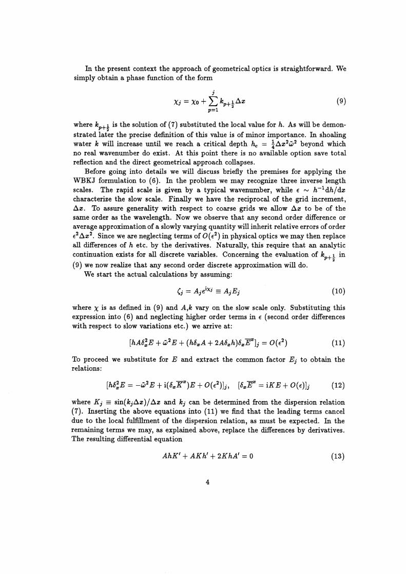
Figlll"e 1: Definition sketch of geometry and wave field.

where the hyphen indicates differentiation with respect to :z:, is easily integrated and the solution for A can be recasted into the very simple form:

(14)

where B is a constant and he is the tlll"ning point depth as defined below (9). We note that (14) is a discrete generalization of Greens law and reproduces the latter in the limit ~:z: --+ 0.

3.2 Verification of the discrete optics.

We employ a simple test bathymetry consisting of a flat bottom, h = hz, for 0 < :z: < :z:z, a shoaling region for :z:z < :z: < :z:,. and a shelf of constant depth h,. for :z:,. < :z: < :Z:b.

In the sloping region h is defined as:

. (7r(:z:-:z:z)) h = hz + ( h,. - hz) sm ( ) 2 :z:,.- :z:z

(15)

We note that h is continuously differentiable everywhere. In the deep region we specify an incident periodic wave of amplitude 1 and frequency w. A definition

5

sketch of the geometry and wave is given in figure 1. To reproduce exactly the steady discrete solution in an infinite domain we invoke a mixed input /radiation condition at ;:c = 0:

(16)

that corresponds to an incident wave of unitary amplitude and the radiation condition

(17)

at ::c = ::cb = N a::c. Naturally, kz and kr fulfill the dispersion relation in the two homogeneous regions respectively. H hr < he (17) must be replaced by

(18)

where kr this time is given by (8). After solving the complex tridiagonal set (6) with the appropriate boundary con­

ditions we extract the amplitude, defined as (a = 1(1, and the amplitude of the reflected wave

Ar = ~~(wcoskza::c)- 1 [iw-r + cos(~kza::c)hft5:~:(]~~ (19)

In figure 2 we have compared the discrete generalization of Greens law, (14), to the exact discrete solution obtained from (6) and the boundary conditions (16), (17). The incident wave has period 8 and hz = 1. For ;:c < ::cz this corresponds to moderately short wave as far as the grid resolution is concerned. For the long slope (::cr- ;:cz = 200) in 2(a) we obtain perfect agreement. In fact, (14) is very good also for the short slope in 2(b) where the the ratio (::cr- ::cz) is as small as 10. However, even if hard to see directly from the figure, the deviations are larger than for the long slope and seem to stem from reflections mainly. The reflection factor Ar is depicted as function of hr in figure 3 for both slope widths. We note that there is no noticeable reflection before hr is very close to he for the long slope.

In figure 4 we have depicted (a for a case with hr < he. We observe the amplitude envelope of a standing wave for h > he and an exponentially decaying tail for h < he.

In this section we have presented a discrete optics for one simple and basic case only. However, a number of extensions are readily available, some of which are presented in the next section.

4 Extensions of the discrete optics.

4.1 Alternative discretizations.

We have employed the scheme of section 3.1 to few other numerical methods than the one given in 2.2. The idea is simply to demonstrate the generality of the results and we find indeed that a stopping depth he exists and that the law (14) is valid for all the discretizations investigated.

6

2.0

1.8

1.6

<

1.4

1.2

1.0

0

num conv.

1.5

1.4

1.3 <

1.2

1.1

1.0

0

num conv.

50

5

100 X

+ + WBKJ • Green

150 200

,/, 1l- -k- -tc- -)If- -)14--M- )C

,•

' I

10 X

' ' ' "' '

I '

+ + WBKJ • Green

15 20

Figure 2: Amplifications of periodic waves incident on a slope. The slope starts at Zz = 5, the grid increment is Lla: = 1 and the incident wave has amplitude 1 and period 27r jw = 8, which imply a stopping depth he = 0.1464. The Upper panel: hr = 0.2, Zr - Zz = 200; Lower panel: hr = 0.3, Xr - a:z = 10. The fully drawn lines are the exact discrete solution, (a, while the '+' marks indicate the discrete WBKJ solution. For comparison we have also depicted the converged ( Lla: --+ 0) discrete solutions with dashed line and Green's law with 'x' marks.

7

1.0

0.8

0.6 <

0.4

0.2

0.0

0.12

I I I I I

\ \

I \ I ', I , , ~~ ~~~~~~~~~ ~----------~~~~~~~------

0.16 0.20 0.24 0.28

Figure 3: Reflection factor A,. for .dz = 1 as function of h,. for z,. - zz = 200 (solid line) and z,.- zz = 10 (dashed) line. The vertical line indicates he= 0.1464.

6

5

4

...J3

2

0

0 10 20 30 40 50 60 70 X

Figure 4: The amplitude (a as function of z for .dz = 1, z,. - a:z = 200, a:z = 5 and a shelf depth h,. = 0.137 that is slightly less than he = 0.1464. The vertical dashes at z = 51.66 indicate the position of h = he. We note that the slightly ragged appearance of the amplitude envelope for h > he is due to the limited resolution.

8

4.1.1 The Crank-Nicholson method.

For the 2-D hydrostatic equations one realization of the technique yields the difference equations:

[ " _ -" (....-a:h -t)](n+~). Vt'TJ- Oz U j 1 [" - " -t] ( n+ ~) VtU - -Oz'TJ . 1 •

J+:a (20)

We note that the method is staggered in space but not in time. The same steps that previously lead to (7) and (6) will reproduce these equations identically, save that w must be redefined according to: w = ~t tan w~t. Therefore the rest of the calculation will repeat; we reproduce (14) but find a larger he.

4.1.2 Finite element methods.

Two relevant finite element formulations will also be briefly discussed. Both methods are based on the same staggered temporal grid as the difference method in section 2.2. The main difference between element and difference methods for the present type of equations is the occurrence of mass matrices with the former. Often the mass matrices are diagonalized and the standard difference methods are virtually reproduced. Hence, in this section we keep consistent mass matrices.

In the first method we start with equations expressed in terms of the velocity potential ¢:

a'TJ = -~ (ha¢)' at az az

a¢ -=-'TJ at

(21)

We note that differentiation of the right equation, with respect to z, and use of the identity a¢j az = u reproduce the equations employed previously. In the residual formulation the right hand side of the continuity equation is integrated by parts and both form and weight functions are chosen to be piecewise linear. The actual form of the assembled equations depends on the integration rule for the term involving h. However, according to the preceding discussions this will not affect the optical description. Anyway, assuming a piecewise linear fit for h and a uniform grid we obtain assembled equations of the form:

[(1 + ~~z2 o;)ot'TJ = -oz(h-moz¢)]jn+~); [(1 + ~~z2 o;)(ot<P + 'TJ) = o]jn+~). (22)

Elimination of ¢nodes and insertion of a single harmonic for 'fJ now yield an equation like (6) with h replaced by h+ ~~z2w2 . We then reproduce the result (14) with the decreased stopping depth he = ~z 2w2 /12.

In the alternative element approach we start from the velocity based equations, represent 'fJ and u as piecewise constant and linear respectively and invoke constant weight functions for the continuity equation while the weight functions for the mo­mentum equations are still linear. The assembled result is1:

[ " - -" (....-a:h )](n+~). Vt'TJ- Oz U j 1 (23)

1 The mixing of linear and internal, constant form functions corresponds to a staggered grid. To reproduce the former enumeration we define element j according to (j - ~ )~:z: < :z: < (j + ! )~:z:.

9

This time it is convenient to eliminate 1J to obtain a single equation for the spatial variation of u. Noting that an identical equation can be obtained from the other formulation, for the spatial variation of 6m</>, we realize that the same expressions for he and the amplitude, A, must apply also in this case.

4.2 Refraction of oblique waves.

So far all optical theory have been exclusively two-dimensional. When generalizing to non-planar motion we must assume that the amplitude factor ( is a function of both z andy and (6) is replaced by

(24)

For single harmonics on constant depth we obtain the dispersion relation

(25)

where l is the y component of the wavenumber and lis defined in analogy with k. A simple generalization of the previous results is obtained when the depth vary in the z direction only. We may then assume (j,p = ei exp(ilpdy) where lis constant. The stopping depth then becomes:

dz2w2

he= -4 + dz2l 2

(26)

From (24) it readily follows that e fulfills an equation like (6) with w2 modified to w2 - hl2 . Repeating the steps that led from (6) to (14) we now obtain a slightly more complicated expression:

( hl2 )-! ( dz 2 _ 2 -2 )-t A= B 1- w2 h- - 4-(w -hi ) (27)

Again we observe that A becomes infinite when h -+ he. For a general depth distribution we have a much more complicated geometrical

optics. We define wave number components according to:

(28)

In addition to the consistency relation

(29)

we also demand fulfillment of the dispersion relation

(30)

10

Due to the slow variation of the wavenumber and depth this will differ from (25) to order €2 and may consequently be replaced by the latter. Likewise, (29) can be replaced by the corresponding differential equation. Provided there exists a unique solution of (28) and {30), or their replacements, substitution into (24) yields:

(31)

where L is defined in analogy with K and r, fare the unit vectors parallel to the principal axes. Equation ( 31) clearly has the form of an energy conservation equation, with a flux in the direction given by K?: + Lf. It is noteworthy that this is also the orientation of the formal group velocity, 2g = ?:8w I 8-;e + f8w I 8y, as can be seen by differentiation of ( 25).

From the dispersion relation we also find an lower bound for the stopping depth

.6.z2 .6.y2w2 h > --:-.,....---::-"---,----::7'

e - 4( .6.z2 + _6.y2) (32)

The above example demonstrates that this criterion generally is too weak. It is must also be expected that he will vary locally according to the topography.

4.3 Non-uniform grids.

The optical results may readily be modified to apply also to gently varying orthogonal grids. For simplicity we confine ourselves to one horizontal dimension and define a transformation ;e = z(O'). Skipping the details we find that (6) may be replaced by

(33)

where the stretch factor 1 = dO" I d;e is assumed to be available at TJ nodes only. However, due to the slow variation of 1 other arrangements will yield the same optical solution. The local dispersion relation now becomes k = w2 l(h1 2 ) where k is defined as the rate of change of the phase function with respect to 0'. A stopping point appear when h = he = w2 .6.0'2 I ( 412). With this definition of he we again reproduce (14) by application of the WBKJ method.

4.4 Local behaviour at the stopping depth.

At the critical depth, h = he, the fast scale variation of the solution of (6) shifts from purely oscillatory to oscillatory with an exponential decay. At such a points, often referred to as a turning point, we may often find a local solution that can be matched asymptotically to the WBKJ solution.

We first note that (7) and (8) imply that k ---+ 7r I .6.-;e as h---+ he from both sides. Hence, the rapid variation does not vanish at the turning point, but the solution of section 3.1 still becomes invalid since K approaches zero at h = he. Instead we seek a local solution through inferring:

{34)

11

where r is a real number defining the critical point and we assume he~ K-Llz(j- r). Substitution into ( 6) then yields:

We then use the relation between he and w, discard higher order terms, and replace differences associated with slow variation by derivatives and obtain:

h D" D' 4s D--K, --- -0 e ,::l;z:2 (36)

where the hyphens denote derivation with respect to s = K-Llz (j - r). A rescaling reveals that the term involving the first derivative may be neglected and we reproduce Airys equation. Requiring that the solution decays as z -+ oo we then find:

(37)

Comparing asymptotic expansions of D as s -+ -oo to leading order behaviour of the WBKJ solution as h -+ h"t we find that an asymptotic match can be performed. However, we omit the tedious details.

5 Concluding remarks.

For difference and element methods there seems to be a well defined stopping depth, he, for a given harmonic wave incident on a coast. In the case of normal incidence

1 we obtain a modified Green's law A"' (h- he)-i where A is the amplitude. Hence, a single harmonic is over-amplified in a numerical model, until the stopping depth is reached and the wave is reflected. Consequently, the underestimation of tsunami heights for coarse grids, as reported in [3], must be explained by numerical dispersion and, to a lesser extent, reflection of the shorter components in the spectrum due to existence of a nonzero he. Moreover, we must expect that a narrow banded swell incident will be over-amplified in shallow water.

Comparing the "discrete Green's law" with exact discrete solutions we obtain excellent agreement. The ideas of a discrete optical theory is readily extended to oblique incidence and non-uniform grids.

The presented work has been carried out under the GITEC (Genesis and Impact of Tsunamis on European Coasts) project that is funded by the European Commission and Norwegian Research Council.

References

[1] Mei, C.C., 1989 The applied dynamics of ocean surface waves. Advanced Series on Ocean Engineering Vol.I, 740 pp. World Scientific, London.

12

[2] Mesinger F., Arakawa A. 1976 Numerical methods used in atmospheric models. GARP, Publ. Ser. WMO 17 64 pp.

[3] Pedersen G. 1995 Grid effects on tsunamis in nearshore regions. University of Oslo, Research Report in Mechanics 1

13