an object description and categorization … · bust to partial occlusion, noise, rotation and...
TRANSCRIPT

AN OBJECT DESCRIPTION
AND CATEGORIZATION METHOD
BASED ON
SHAPE AND APPEARANCE
FEATURES
by
M.Sc. Leonardo Chang Fernandez
A THESIS SUBMITTED IN PARTIAL FULFILLMENT OFTHE REQUIREMENTS FOR THE DEGREE OF
DOCTOR IN COMPUTER SCIENCE
at the
Instituto Nacional de Astrofısica, Optica y ElectronicaTonantzintla, Puebla, Mexico
2015
Advisors:
Dr. Miguel Octavio Arias Estrada, INAOE, MexicoDr. Luis Enrique Sucar Succar, INAOE, MexicoDr. Jose Hernandez Palancar, CENATAV, Cuba
c⃝INAOE 2015The author hereby grants to INAOE permission to
reproduce and to distribute publicly paper and electroniccopies of this thesis document in whole or in part.


A mis padres y hermanaeste minusculo paso
en mi caminoa ser como ustedes.


Agradecimientos
Quiero expresar mis mas sinceros agradecimientos a mis asesores Dr. Luis Enrique Sucar,Dr. Miguel Arias Estrada y Dr. Jose Hernandez Palancar, por todo el apoyo, guıa yconocimiento brindados durante el desarrollo de esta investigacion. Sus ensenanzas hansido fundamentales para el desarrollo de esta tesis doctoral y para el mıo propio comoinvestigador.
A mis sinodales Dra. Angelica Munoz Melendez, Dr. Eduardo Morales Manzanares, Dr.Jesus Antonio Gonzalez Bernal, Dr. Hugo Jair Escalante Balderas y Dr. Gustavo OlagueCaballero por sus certeras observaciones y sugerencias que ayudaron a mejorar la calidadde esta tesis.
Al CENATAV, por formarme como profesional e investigador, por darme un lugar dondesentirme como en casa.
A Shul, por su inagotable energıa en la tarea de convertirnos en mejores investigadores yprofesionales. A Isneri, por su apoyo y ejemplo.
A mis padres, por toda la sabidurıa, educacion, consejos y amor que me han brindado,ustedes son lo maximo.
A mi hermana, por ser mi mejor amiga, mi complice incondicional, mi complemento.
A mi cunado Ariel, por cuidar y amar a mi ser mas querido. Tambien por las construc-ciones de las que me he librado durante este perıodo.
A toda mi familia y amigos, por hacer mi vida muy feliz.
A todos mis companeros del CENATAV, todos han sido parte de esta etapa de mi viday me han ayudado de una forma u otra. En especial a Yoanna, Airel, Heydi, Annette,Noslen, Yenisel, Nelson, Raudel por todo lo que hemos compartido cada dıa.
A mis amigos-hermanos, a Alfre por siempre estar ahı, ya son casi 20 anos bro! Al flaco porser un amigo incondicional y tambien por la parte que compartimos de la investigacion. A
Jasan que aunque lejos y distantes seguimos siendo hermanos. A mis hermanos de Ciego,Andres, Tavo y Migue en quienes gracias a esta tesis encontre excelentes amigos.
A todos aquellos que conocı durante mis dıas en Mexico, hicieron de esto una experienciaexcepcional.
Al INAOE por brindarme un espacio para desarrollar mis estudios, no hubiera preferidootro. A todos los investigadores de la Coordinacion de Ciencias Computacionales, enespecial al Dr. Ariel Carrasco Ochoa, quien siempre nos ha brindado su ayuda y hospi-talidad.
Al CONACYT (a traves de la beca No. 240251) por brindarme los medios materiales yeconomicos para realizar esta investigacion.
A mi Patria y a mi bandera.
Leonardo Chang Fernandez.Tonantzintla, Puebla. 15 de Junio de 2015.

Abstract
Object recognition in images is one of the oldest problems in Computer Vision. Inthis thesis, we focus on the problem of category-level object recognition, based on theuse of shape features as a more generic representation of object classes than appearancefeatures, while the latest are used as second-level features.
In this research work we propose an invariant shape feature extraction, description andmatching method for binary images, named LISF. The proposed method extracts localfeatures from the contour to describe shape and these features are later matched globally.Combining local features with global matching allows us to obtain a trade-off betweendiscriminative power and robustness to noise and occlusion in the contour. The proposedextraction, description and matching methods are invariant to rotation, translation andscale, and present certain robustness to partial occlusion. The conducted experimentsshowed that, for larger occlusion levels, the better was the performance of LISF withrespect to other popular shape description methods, with about 20% higher bull’s eyescore and 25% higher accuracy in classification in images with a 60% occlusion. Also, wepresent a massively parallel implementation in GPU of LISF, which achieves a speed-upof up to 34x.
In order to deal with the intrinsic problems derived from using edges extracted fromreal images, in this thesis we propose a shape descriptor, named OCTAR, that is particu-larly suitable for partial shape matching of open/closed contours extracted from edgemapimages. Based on this descriptor, we also propose a partial shape matching method ro-bust to partial occlusion, noise, rotation and translation. Our approach allows to combineshape and appearance through the evaluation of object detection hypothesis based on itsappearance, providing more distinctiveness. The conducted experiments showed compet-itive results compared to the state of the art, in both binary and gray scale images.
Further, we introduce three properties and their corresponding quantitative evalu-ation measures to assess the ability of a visual word to represent and discriminate anobject class, in the context of the BoW approach. Based on these properties, we pro-pose a methodology for reducing the size of the visual vocabulary, retaining those visualwords that best describe an object class. Reducing the vocabulary will provide a morereliable and compact image representation. This representation is used by the OCTARmethod to evaluate the appearance of object detection hypotheses. Experiments wereperformed using different size vocabularies, different appearance descriptors, differentweighting schemas, and different classifiers, which showed that using our reduced vocab-ulary improves the classification performance with a significant reduction of the imagerepresentation size.
i

Resumen
El reconocimiento de objetos en imagenes es uno de los problemas mas antiguos enel campo de la vision por computadoras. En esta tesis, con el objetivo de lograr mejoresresultados en la categorizacion de objetos, se utilizan caracterısticas de forma como unarepresentacion mas generica de los objetos que la brindada por las caracterısticas deapariencia, las que son usadas como caracterısticas de segundo nivel.
En esta tesis se propone un metodo, denominado LISF, para la extraccion, descripciony comparacion de caracterısticas de forma para imagenes binarias. LISF extrae y describela forma de manera local pero halla correspondencias usando informacion global con elfin de obtener un balance entre el poder discriminativo y la robustez al ruido y oclusionparcial en el contorno. Los experimentos realizados muestran que para mayores nivelesde oclusion en la forma, mejores son los resultados de LISF con respecto a otros metodosdel estado del arte, con mejorıas del 20% en la medida bull’s eye y del 25% de exactituden la clasificacion para una oclusion del 60%. Tambien, se propone una implementacionmasivamente paralela en GPU de LISF, que alcanza una aceleracion de hasta 34x.
Para poder lidiar con los problemas intrınsecos del uso de la informacion de formaobtenida a partir de bordes extraıdos de imagenes reales, como parte de este trabajo sepropone un descriptor de forma, al que denominamos OCTAR, particularmente disenadopara hallar correspondencias parciales entre contornos abiertos o cerrados extraıdos deimagenes de mapas de bordes. Basados en este descriptor, se propuso ademas un metodode comparacion parcial de formas, que es robusto a la oclusion parcial, ruido, rotaciony traslacion. Este metodo permite combinar la forma con la apariencia a partir de laevaluacion de hipotesis de objetos basados en la informacion de apariencia, brindandomayor poder discriminativo. Los experimentos realizados muestran su efectividad tantoen imagenes binarias como en imagenes reales.
Por ultimo, se proponen tres propiedades y sus correspondientes medidas de evaluacioncualitativas para expresar la habilidad de una palabra visual de representar y discriminaruna categorıa de objetos, dentro del enfoque de bolsas de palabras visuales. Basado enestas propiedades, se propone una metodologıa para reducir el tamano de los vocabula-rios visuales, obteniendo vocabularios mas compactos pero que a su vez mejor describeny discriminan a las categorıas de objetos. Esta representacion es usada para evaluar laapariencia en el metodo OCTAR. Los experimentos, que se realizaron usando diferentestamanos de vocabularios, varios descriptores de apariencia, diferentes esquemas de pe-sado y diferentes clasificadores, mostraron que usando nuestros vocabularios reducidos seobtenıan mejores resultados en la categorizacion que usando los vocabularios completos,con una significativa reduccion en el tamano de la representacion de las imagenes.
ii

Contents
1 Introduction 1
1.1 Problem Description . . . . . . . . . . . . . . . . . . . . . . . . . . . . . . 4
1.2 Objectives . . . . . . . . . . . . . . . . . . . . . . . . . . . . . . . . . . . . 6
1.3 Contributions . . . . . . . . . . . . . . . . . . . . . . . . . . . . . . . . . . 7
1.4 Thesis Structure . . . . . . . . . . . . . . . . . . . . . . . . . . . . . . . . . 8
2 Related Work 10
2.1 Object Recognition Evolution . . . . . . . . . . . . . . . . . . . . . . . . . 10
2.2 Shape-based Category-level Object Recognition . . . . . . . . . . . . . . . 13
2.3 Appearance-based Category-level Object Recognition . . . . . . . . . . . . 14
2.4 Shape Feature Descriptors . . . . . . . . . . . . . . . . . . . . . . . . . . . 16
2.5 Triangle Area-based Shape Feature Descriptors . . . . . . . . . . . . . . . 18
2.6 Building More Discriminative and Representative Visual Vocabularies . . . 20
2.7 Summary . . . . . . . . . . . . . . . . . . . . . . . . . . . . . . . . . . . . 22
3 The Invariant Local Shape Features Method 23
3.1 Proposed Local Shape Feature Descriptor . . . . . . . . . . . . . . . . . . . 24
3.1.1 Feature Extraction . . . . . . . . . . . . . . . . . . . . . . . . . . . 24
3.1.2 Feature Description . . . . . . . . . . . . . . . . . . . . . . . . . . . 26
3.1.3 Robustness and Invariability Considerations . . . . . . . . . . . . . 26
3.2 Proposed Feature Matching . . . . . . . . . . . . . . . . . . . . . . . . . . 28
3.2.1 Finding Candidate Matches . . . . . . . . . . . . . . . . . . . . . . 28
3.2.2 Rejecting Casual Matches . . . . . . . . . . . . . . . . . . . . . . . 30
iii

3.3 Efficient LISF Feature Extraction and Matching . . . . . . . . . . . . . . . 32
3.3.1 Implementation of Feature Extraction using CUDA . . . . . . . . . 32
3.3.2 Implementation of Feature Matching using CUDA . . . . . . . . . . 33
3.4 Experimental Results . . . . . . . . . . . . . . . . . . . . . . . . . . . . . . 35
3.4.1 Shape Retrieval and Classification Experiments . . . . . . . . . . . 35
3.4.2 Efficiency Evaluation . . . . . . . . . . . . . . . . . . . . . . . . . . 39
3.5 Summary . . . . . . . . . . . . . . . . . . . . . . . . . . . . . . . . . . . . 41
4 The Open/Closed Contours Triangle Area Representation Method 42
4.1 Proposed Shape Descriptor . . . . . . . . . . . . . . . . . . . . . . . . . . . 44
4.2 Proposed Partial Shape Matching Method . . . . . . . . . . . . . . . . . . 46
4.3 Object Hypotheses Formation and Evaluation . . . . . . . . . . . . . . . . 48
4.3.1 Covering Criterion . . . . . . . . . . . . . . . . . . . . . . . . . . . 50
4.3.2 Object Hypothesis Contour Estimation Criterion . . . . . . . . . . 50
4.3.3 Fitted Object Hypothesis Criterion . . . . . . . . . . . . . . . . . . 51
4.3.4 Appearance-based Evaluation Criterion . . . . . . . . . . . . . . . . 52
4.4 Experimental Results . . . . . . . . . . . . . . . . . . . . . . . . . . . . . . 53
4.4.1 Performance Evaluation on Real Scenes . . . . . . . . . . . . . . . . 53
4.4.2 Performance Evaluation on Occluded Shapes . . . . . . . . . . . . . 56
4.5 Summary . . . . . . . . . . . . . . . . . . . . . . . . . . . . . . . . . . . . 58
5 Improving Visual Vocabularies 59
5.1 Proposed Method . . . . . . . . . . . . . . . . . . . . . . . . . . . . . . . . 61
5.1.1 Inter-class Representativeness Measure . . . . . . . . . . . . . . . . 62
5.1.2 Intra-class Representativeness Measure . . . . . . . . . . . . . . . . 62
5.1.3 Inter-class Distinctiveness Measure . . . . . . . . . . . . . . . . . . 65
5.1.4 On Ranking and Reducing the Size of Visual Vocabularies . . . . . 66
5.2 Experimental Evaluation . . . . . . . . . . . . . . . . . . . . . . . . . . . . 67
5.2.1 Assessing the Validity in a Classic BoW-based Classification Task . 68
5.2.2 Comparison with Other Kinds of Feature Selection Algorithms . . . 76
iv

5.2.3 Computation Time of the Visual Vocabulary Ranking . . . . . . . . 78
5.3 Summary . . . . . . . . . . . . . . . . . . . . . . . . . . . . . . . . . . . . 78
6 Conclusions 79
6.1 Summary and Conclusions . . . . . . . . . . . . . . . . . . . . . . . . . . . 79
6.2 Main Contributions . . . . . . . . . . . . . . . . . . . . . . . . . . . . . . . 80
6.3 Future Work . . . . . . . . . . . . . . . . . . . . . . . . . . . . . . . . . . . 81
6.4 Publications . . . . . . . . . . . . . . . . . . . . . . . . . . . . . . . . . . . 82
References 84
A The Mann-Whitney Test 99
B Acronyms 101
C Notations 103
v

List of Figures
1.1 Object recognition. . . . . . . . . . . . . . . . . . . . . . . . . . . . . . . . 2
2.1 Evolution of object recognition. . . . . . . . . . . . . . . . . . . . . . . . . 11
3.1 Detection of contour fragments in LISF method. . . . . . . . . . . . . . . . 25
3.2 LISF contour fragment descriptor. . . . . . . . . . . . . . . . . . . . . . . . 27
3.3 LISF contour fragment scale and orientation. . . . . . . . . . . . . . . . . . 29
3.4 Casual matches rejection stage of the LISF method. . . . . . . . . . . . . . 31
3.5 Matches between local shape descriptors in two images using LISF method. 32
3.6 Overview of the proposed LISF feature comparison method in GPU. . . . . 34
3.7 Example images and categories from the Shapes99, Shapes216 and the
MPEG-7 datasets. . . . . . . . . . . . . . . . . . . . . . . . . . . . . . . . 35
3.8 Example images from the MPEG-7 dataset with different levels of occlusion
used in the experiments. . . . . . . . . . . . . . . . . . . . . . . . . . . . . 36
3.9 Bull’s eye score comparison between LISF, shape context, Zernike moments
and Legendre moments. . . . . . . . . . . . . . . . . . . . . . . . . . . . . 37
3.10 Top 5 retrieved images by LISF and its similarity score. . . . . . . . . . . . 38
3.11 Classification accuracy comparison between LISF, shape context, Zernike
moments and Legendre moments. . . . . . . . . . . . . . . . . . . . . . . . 39
3.12 Computation time and achieved speed-up by the proposed massively par-
allel implementation of LISF in CUDA. . . . . . . . . . . . . . . . . . . . . 40
4.1 Problems derived from using edgemaps extracted from real images. . . . . 43
4.2 The OCTAR descriptor computation. . . . . . . . . . . . . . . . . . . . . . 45
vi

4.3 The OCTAR descriptor self-containing property. . . . . . . . . . . . . . . . 46
4.4 The OCTAR partial shape matching process. . . . . . . . . . . . . . . . . . 48
4.5 OCTAR spatial relation constraints graph. . . . . . . . . . . . . . . . . . . 49
4.6 Extended OCTAR descriptor for contours spatial configuration. . . . . . . 49
4.7 Example images from the ETHZ Shape Classes dataset. . . . . . . . . . . . 53
4.8 Example edgemap images from the ETHZ Shape Classes dataset. . . . . . 54
4.9 Example image from the Shapes216 dataset with different levels of occlusion. 56
4.10 Bull’s eye score comparison between OCTAR, shape context and IDSC. . . 57
5.1 BoW approach overview. . . . . . . . . . . . . . . . . . . . . . . . . . . . . 60
5.2 Examples of M1 measure values. . . . . . . . . . . . . . . . . . . . . . . . 63
5.3 Examples of M2 measure values. . . . . . . . . . . . . . . . . . . . . . . . 64
5.4 Example of M3 measure for two visual words. . . . . . . . . . . . . . . . . 66
5.5 Mean classification accuracy results for SVM cross-validation on the
Caltech-101 dataset. . . . . . . . . . . . . . . . . . . . . . . . . . . . . . . 71
5.6 Mean classification accuracy results for KNN cross-validation on the
Caltech-101 dataset. . . . . . . . . . . . . . . . . . . . . . . . . . . . . . . 72
5.7 Mean classification accuracy results for SVM cross-validation on the Pascal
VOC 2006 dataset. . . . . . . . . . . . . . . . . . . . . . . . . . . . . . . . 73
5.8 Mean classification accuracy results for KNN cross-validation on the Pascal
VOC 2006 dataset. . . . . . . . . . . . . . . . . . . . . . . . . . . . . . . . 74
5.9 Comparison of classification accuracy results with the state of the art. . . . 77
vii

List of Tables
3.1 Average feature extraction and matching time for two images of the
MPEG7 database, in seconds. . . . . . . . . . . . . . . . . . . . . . . . . . 39
4.1 Comparison of interpolated average precision (AP) on the ETHZ Shape
Classes dataset. . . . . . . . . . . . . . . . . . . . . . . . . . . . . . . . . . 55
4.2 Comparison of classification accuracy on the ETHZ Shape Classes dataset. 55
4.3 OCTAR average feature extraction and matching time comparison. . . . . 57
5.1 Summarized classification accuracy results for the Caltech-101 dataset. . . 75
5.2 Summarized classification accuracy results for the Pascal VOC 2006 dataset. 75
5.3 Computation time of visual vocabulary ranking compared to vocabulary
building. . . . . . . . . . . . . . . . . . . . . . . . . . . . . . . . . . . . . . 75
viii
Chapter 1
Introduction
Object recognition is one of the oldest problems in the field of Computer Vision. However,
it still remains an open problem. Object recognition can be divided into two distinct
groups:
• Specific object recognition: Let us assume the problem of finding John’s car in
an image. In this case, the object we are looking for is a car, but the key here is
that we are not looking for any car, we are looking for an object that has unique
and distinctive features, in this case John’s car. (See Figure 1.1 (a))
• Category-level object recognition: This is a more general problem. Following
the same example, the problem here is to detect every car in the image, see Figure
1.1 (b). In this case, we would have to use training data to create a model of a
car able to generalize the class of cars. Then, with this model, detect all objects
and classify them as a car or not. Hence, it follows that the class of objects we
want to recognize can be as specific (e.g., Toyota cars) or as general (e.g., every
ground transportation) as needed. Taking this into account, the case of specific
object recognition could be seen as the more specific case of category-level object
recognition.
In the present doctoral research, we focus on the problem of category-level object
recognition (also referred to as object categorization, object class recognition, generic
object recognition and classification of objects). More formally, it can be defined as:
1

John’s car
(a)
(b)
Figure 1.1: Object recognition could be seen under two different groups: (a) specificobject recognition and (b) category-level object recognition.
given a number of training images from a category or a class of objects, recognize unseen
instances of that category and assign the appropriate label to them.
In recent years, the field of specific object recognition has made significant progress
with the emergence of local appearance-based features (e.g., SIFT (Lowe, 2004), SURF
(Bay et al., 2008), ORB (Rublee et al., 2011), Harris-Affine (Mikolajczyk and Schmid,
2002)(Mikolajczyk, 2004), Hessian-Affine (Mikolajczyk and Schmid, 2002)(Mikolajczyk,
2004), MSER (Matas, 2004)). Local appearance-based features have proven to be very
2
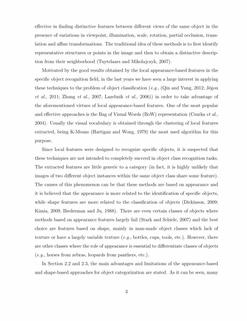
effective in finding distinctive features between different views of the same object in the
presence of variations in viewpoint, illumination, scale, rotation, partial occlusion, trans-
lation and affine transformations. The traditional idea of these methods is to first identify
representative structures or points in the image and then to obtain a distinctive descrip-
tion from their neighborhood (Tuytelaars and Mikolajczyk, 2007).
Motivated by the good results obtained by the local appearance-based features in the
specific object recognition field, in the last years we have seen a large interest in applying
these techniques to the problem of object classification (e.g., (Qin and Yung, 2012; Jegou
et al., 2011; Zhang et al., 2007; Lazebnik et al., 2006)) in order to take advantage of
the aforementioned virtues of local appearance-based features. One of the most popular
and effective approaches is the Bag of Visual Words (BoW) representation (Csurka et al.,
2004). Usually the visual vocabulary is obtained through the clustering of local features
extracted, being K-Means (Hartigan and Wong, 1979) the most used algorithm for this
purpose.
Since local features were designed to recognize specific objects, it is suspected that
these techniques are not intended to completely succeed in object class recognition tasks.
The extracted features are little generic to a category (in fact, it is highly unlikely that
images of two different object instances within the same object class share some feature).
The causes of this phenomenon can be that these methods are based on appearance and
it is believed that the appearance is more related to the identification of specific objects,
while shape features are more related to the classification of objects (Dickinson, 2009;
Kimia, 2009; Biederman and Ju, 1988). There are even certain classes of objects where
methods based on appearance features largely fail (Stark and Schiele, 2007) and the best
choice are features based on shape, mainly in man-made object classes which lack of
texture or have a largely variable texture (e.g., bottles, cups, tools, etc.). However, there
are other classes where the role of appearance is essential to differentiate classes of objects
(e.g., horses from zebras, leopards from panthers, etc.).
In Section 2.2 and 2.3, the main advantages and limitations of the appearance-based
and shape-based approaches for object categorization are stated. As it can be seen, many
3

of the limitations of one of theses approaches are complemented by the other advantages.
In this doctoral research, we propose to combine appearance and shape features by
taking advantage of each of these representations in the classification of objects. With
the combination of both kind of features we expect better classification results than when
using these features separately.
On the other hand, historically, the researchers in this area have been more focused
on obtaining accurate methods leaving aside efficiency. However, the latter has become
an increasingly important issue, mainly motivated by the need to recognize object classes
in real-time applications or other applications where execution time is a critical resource.
An example of this would be the representation of visual information according to
the MPEG-7 standard (Martınez, 2004). The main difference of this standard to its
predecessor MPEG-4 is that it includes labelling of multimedia content through metadata,
including the category to which each object belongs. Another example could be robotics
or video surveillance applications where certain categories of objects have to be found in
a scene in real time (∼ 30 fps).
A technology that has proven to be successful in accelerating several computing tasks
is the use of GPUs (Graphics Processing Units). GPUs are processors initially designed to
perform the calculations involved in the generation of interactive 3D graphics. However,
some of their main characteristics (low price in relation to its computing power, high
parallelism capabilities, floating point operations optimization) have led the scientific
community to extend their use to a wider range of computing tasks, to what has been
called General-Purpose Computing on Graphics Processing Units (GPGPU).
In this dissertation, we also propose a massively parallel GPU implementation in
CUDA, to ensure an acceleration of the recognition of classes of objects in images that
favor their use in applications where time is a critical factor.
4

1.1 Problem Description
During the historical development of object recognition there has been a trend towards
recognizing specific objects, leaving aside the recognition of object classes, so that the
greatest achievements and developments have been reached in the first of these. Having
now attained great progress in recognizing specific objects (emergence of the appearance-
based invariant local features, e.g., SIFT, SURF, ORB, Harris-Affine, Hessian-Affine,
MSER), a boom in applying appearance-based local features techniques to the more gen-
eral problem of object classification has been seen, constituting these schemas the state
of the art in the subject.
From the above, it is suspected that appearance-based local features methods can
not completely succeed, because these methods from their theoretical conception were
designed to recognize specific objects and the features extracted are little generic to a
category. Local appearance features are structures on the objects that are present in
different views of the same object, but in their theoretical basis there is nothing to indicate
that these features are capable of abstracting the appearance of an object class (beyond a
specific object), in fact, it is very unlikely that two images of different objects belonging
to the same class share a local appearance feature.
What we propose in this thesis, and that has become a trend in recent research, is
returning to the use of shape as a more generic representation of objects. Also, by combin-
ing shape features with the progress made in the description of the appearance, we expect
to be able to achieve better results in object categorization. Throughout the evolution of
object recognition, shape features have shown greater ability to represent object categories
than appearance features. Furthermore, studies on how humans identify object categories
have shown that humans rely primarily on shape features, leaving appearance features as
a second-level features (Biederman and Ju, 1988). On the other hand, recent studies on
the use of appearance have shown its importance in object categorization, specifically in
object classes with similar shape (e.g., cougar vs. panther, zebra vs. horse, etc.), hence
the need to combine together shape and appearance.
5
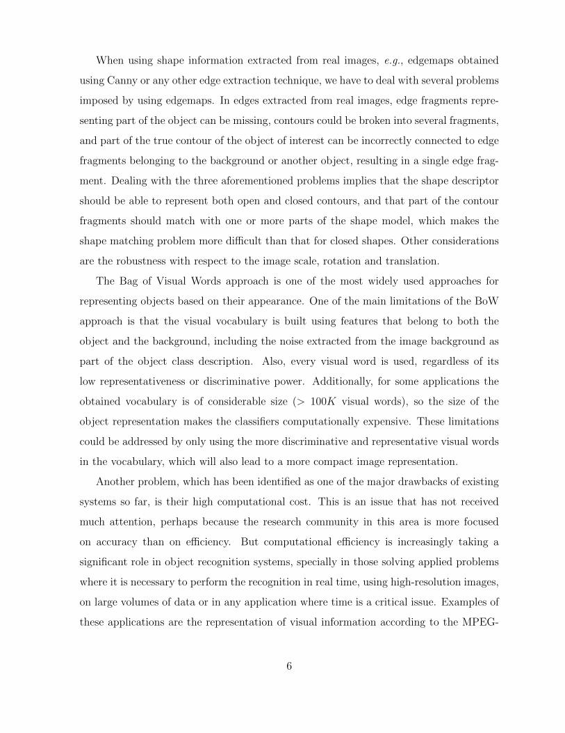
When using shape information extracted from real images, e.g., edgemaps obtained
using Canny or any other edge extraction technique, we have to deal with several problems
imposed by using edgemaps. In edges extracted from real images, edge fragments repre-
senting part of the object can be missing, contours could be broken into several fragments,
and part of the true contour of the object of interest can be incorrectly connected to edge
fragments belonging to the background or another object, resulting in a single edge frag-
ment. Dealing with the three aforementioned problems implies that the shape descriptor
should be able to represent both open and closed contours, and that part of the contour
fragments should match with one or more parts of the shape model, which makes the
shape matching problem more difficult than that for closed shapes. Other considerations
are the robustness with respect to the image scale, rotation and translation.
The Bag of Visual Words approach is one of the most widely used approaches for
representing objects based on their appearance. One of the main limitations of the BoW
approach is that the visual vocabulary is built using features that belong to both the
object and the background, including the noise extracted from the image background as
part of the object class description. Also, every visual word is used, regardless of its
low representativeness or discriminative power. Additionally, for some applications the
obtained vocabulary is of considerable size (> 100K visual words), so the size of the
object representation makes the classifiers computationally expensive. These limitations
could be addressed by only using the more discriminative and representative visual words
in the vocabulary, which will also lead to a more compact image representation.
Another problem, which has been identified as one of the major drawbacks of existing
systems so far, is their high computational cost. This is an issue that has not received
much attention, perhaps because the research community in this area is more focused
on accuracy than on efficiency. But computational efficiency is increasingly taking a
significant role in object recognition systems, specially in those solving applied problems
where it is necessary to perform the recognition in real time, using high-resolution images,
on large volumes of data or in any application where time is a critical issue. Examples of
these applications are the representation of visual information according to the MPEG-
6

7 standard, applications of robotics where the detection of certain object categories is
needed, or video surveillance applications where certain objects must be found to launch
an alarm.
1.2 Objectives
The general objective of this doctoral research is to develop a method for category-level
object recognition in images, based on local shape and appearance features, competitive
against state-of-the-art methods in terms of accuracy, and at the same time more robust
to occlusions.
Our specific objectives are:
1. To propose an invariant shape features extraction, description and matching method
for binary images robust to partial occlusions.
2. To propose a shape descriptor able to deal with the intrinsic problems derived from
using edges extracted from real images.
3. To propose a shape matching method able to deal with the intrinsic problems derived
from using edges extracted from real images and that uses the above descriptor.
4. To propose a method for obtaining a compact, discriminative and representative
appearance BoW-based representation.
5. To propose a method for category-level object recognition that equally favors both
shape and appearance cues, improving the accuracy of reported results.
6. To develop a massively parallel GPU implementation of the most time consuming
parts and exceed by at least 10 times in terms of efficiency the CPU implementation.
1.3 Contributions
The main contribution of this doctoral dissertation is the proposal of a method for
category-level object recognition that favors both shape and appearance cues.
7

We introduce a shape-based object recognition method, named LISF, that is invariant
to rotation, translation and scale, and present robustness to partial occlusion. LISF, for
highly occluded images largely outperformed other popular shape description methods
and retain comparable results for not occluded images. We also propose a massively
parallel implementation in CUDA of the two most time-consuming stages of LISF, i.e.,
the feature extraction and feature matching steps, which achieves speed-ups of up to 32x
and 34x, respectively.
Further, we introduce a shape-based object recognition method, named OCTAR, able
to deal with the intrinsic problems derived from using edges extracted from real images,
i.e., broken and missing edge fragments that represent the target object, edge fragment
wrongly connected to another object or background edges, and background cluttering.
In this method is where the combination of shape and appearance features is performed.
Appearance cues are used as a second-level features. OCTAR, for highly occluded images
largely outperformed other popular shape description methods and retained comparable
results for not occluded images. Also, outperformed other methods in the state of the art
in object detection in real images.
Additionally, we propose three properties and their corresponding quantitative eval-
uation measures to assess the ability of a visual word to represent and discriminate an
object class, in the context of the BoW approach. Also, based on these properties, we
proposed a methodology for reducing the size of the visual vocabulary, retaining those
visual words that best describe an object class. Using our reduced vocabularies the classi-
fication performance is improved with a significant reduction of the image representation
size.
1.4 Thesis Structure
The content of this thesis is organized in six chapters. Chapter 2 points some key issues in
the evolution of the object recognition field that support our proposal. Also, it presents a
critical review of the main approaches in the state of the art of the shape and appearance-
8

based category-level object recognition.
In Chapter 3, we introduce an invariant shape feature extraction, description and
matching method for binary images, named LISF. Also, in this chapter, we propose a
massively parallel implementation in CUDA of the two most time-consuming stages of
LISF, i.e., the feature extraction and feature matching steps. Finally, we present several
experiments to show the robustness of the LISF method to partial occlusion in the shape
and in order to provide an efficiency evaluation of the proposed GPU parallel implemen-
tation.
In Chapter 4, we propose the OCTAR descriptor, a shape descriptor that is particularly
suitable for partial shape matching of open/closed contours extracted from edge map
images, e.g., using Canny or any other edge extraction method from gray or color images.
Based on this descriptor, we also introduce a partial shape matching method robust to
partial occlusion and noise in the extracted contour. In OCTAR we combine shape and
appearance features, specifically by using appearance as a second level feature. Finally,
several experiments to show the advantages of the OCTAR description and matching
method in binary and edge images (extracted from color images) are presented.
In Chapter 5, we introduce three properties and their corresponding qualitative eval-
uation measures to assess the ability of a visual word to represent and discriminate an
object class, in the context of the BoW approach. Also, based on these properties, we
propose a methodology for reducing the size of the visual vocabulary, retaining those vi-
sual words that best describe an object class. Further, we present several experiments in
well-known datasets in order to show that using only the most discriminative and repre-
sentative visual words obtained by our proposed methodology improves the classification
performance.
Finally, Chapter 6 concludes the thesis, and presents our future work, contributions
and the publications obtained as result of this thesis.
9

Chapter 2
Related Work
2.1 Object Recognition Evolution
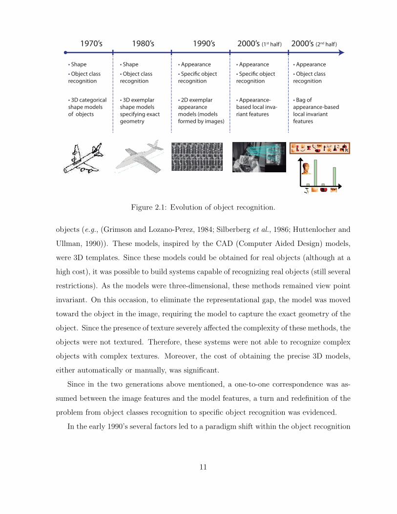
The evolution of object recognition over the past 40 years has followed a very clear path, as
illustrated in Figure 2.1. In the 1970’s, the main research on object recognition focused
on obtaining generic representations of the objects 3D shape. The objects were repre-
sented mostly as construction of volumetric parts, e.g., cylinders (Binford, 1971; Agin
and Binford, 1976; Brooks, 1983), superquadrics (Ferrie et al., 1993; Solina and Bajcsy,
1990; Pentland, 1986; Terzopoulos and Metaxas, 1991), and geons (Biederman, 1985).
The main drawback that these early systems were facing was the representational gap
that existed between the low-level features that could be effectively extracted from the
image and the abstract nature of the model components. Instead of trying to eliminate
this gap by creating more effective mechanisms for abstraction, the trend was to bring
the images closer to the model. Therefore, in order to obtain generic representations of
the objects 3D shape, it was necessary to eliminate the objects surface textures and other
structural details, control the illumination conditions and use more uniform backgrounds.
As a result, the obtained systems were not able to recognize objects in images obtained
in real conditions. However, several basic principles emerged in that decade, such as the
importance of shape, the significance of invariance to viewpoint and the importance of
3D representations, among others.
In the 1980’s, the main trend was to obtain 3D models that represent the exact shape of
10
1970’s 1980’s 1990’s 2000’s (1st half ) 2000’s (2nd half )
• Shape
• Object class
recognition
• 3D categorical
shape models
of objects
• Shape
• Object class
recognition
• 3D exemplar
shape models
specifying exact
geometry
• Appearance
• Speci!c object
recognition
• 2D exemplar
appearance
models (models
formed by images)
• Appearance
• Speci!c object
recognition
• Appearance-
based local inva-
riant features
• Appearance
• Object class
recognition
• Bag of
appearance-based
local invariant
features
Figure 2.1: Evolution of object recognition.
objects (e.g., (Grimson and Lozano-Perez, 1984; Silberberg et al., 1986; Huttenlocher and
Ullman, 1990)). These models, inspired by the CAD (Computer Aided Design) models,
were 3D templates. Since these models could be obtained for real objects (although at a
high cost), it was possible to build systems capable of recognizing real objects (still several
restrictions). As the models were three-dimensional, these methods remained view point
invariant. On this occasion, to eliminate the representational gap, the model was moved
toward the object in the image, requiring the model to capture the exact geometry of the
object. Since the presence of texture severely affected the complexity of these methods, the
objects were not textured. Therefore, these systems were not able to recognize complex
objects with complex textures. Moreover, the cost of obtaining the precise 3D models,
either automatically or manually, was significant.
Since in the two generations above mentioned, a one-to-one correspondence was as-
sumed between the image features and the model features, a turn and redefinition of the
problem from object classes recognition to specific object recognition was evidenced.
In the early 1990’s several factors led to a paradigm shift within the object recognition
11
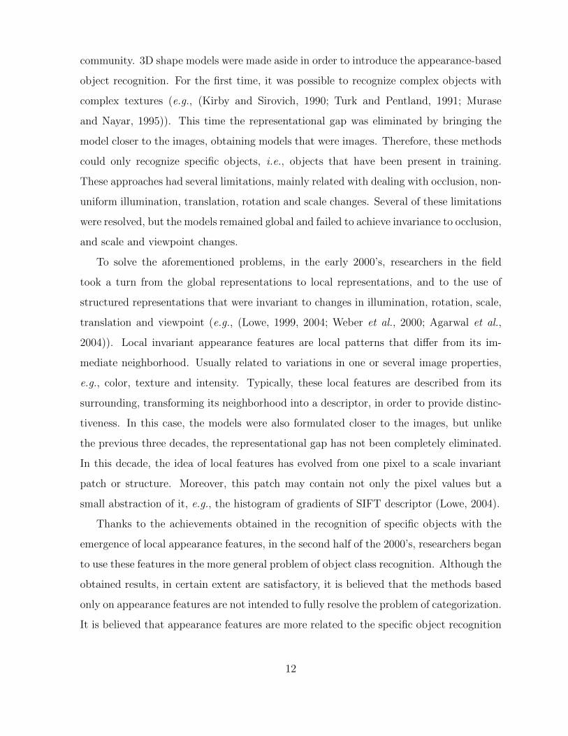
community. 3D shape models were made aside in order to introduce the appearance-based
object recognition. For the first time, it was possible to recognize complex objects with
complex textures (e.g., (Kirby and Sirovich, 1990; Turk and Pentland, 1991; Murase
and Nayar, 1995)). This time the representational gap was eliminated by bringing the
model closer to the images, obtaining models that were images. Therefore, these methods
could only recognize specific objects, i.e., objects that have been present in training.
These approaches had several limitations, mainly related with dealing with occlusion, non-
uniform illumination, translation, rotation and scale changes. Several of these limitations
were resolved, but the models remained global and failed to achieve invariance to occlusion,
and scale and viewpoint changes.
To solve the aforementioned problems, in the early 2000’s, researchers in the field
took a turn from the global representations to local representations, and to the use of
structured representations that were invariant to changes in illumination, rotation, scale,
translation and viewpoint (e.g., (Lowe, 1999, 2004; Weber et al., 2000; Agarwal et al.,
2004)). Local invariant appearance features are local patterns that differ from its im-
mediate neighborhood. Usually related to variations in one or several image properties,
e.g., color, texture and intensity. Typically, these local features are described from its
surrounding, transforming its neighborhood into a descriptor, in order to provide distinc-
tiveness. In this case, the models were also formulated closer to the images, but unlike
the previous three decades, the representational gap has not been completely eliminated.
In this decade, the idea of local features has evolved from one pixel to a scale invariant
patch or structure. Moreover, this patch may contain not only the pixel values but a
small abstraction of it, e.g., the histogram of gradients of SIFT descriptor (Lowe, 2004).
Thanks to the achievements obtained in the recognition of specific objects with the
emergence of local appearance features, in the second half of the 2000’s, researchers began
to use these features in the more general problem of object class recognition. Although the
obtained results, in certain extent are satisfactory, it is believed that the methods based
only on appearance features are not intended to fully resolve the problem of categorization.
It is believed that appearance features are more related to the specific object recognition
12

problem and so shape features with object categorization (Dickinson, 2009; Kimia, 2009;
Biederman and Ju, 1988), as evidenced throughout the evolution of this field when a turn
towards using appearance features, inevitably turned to the recognition of specific objects.
2.2 Shape-based Category-level Object Recognition
Since the beginning of research in the field of object recognition, shape features have
been widely used. The primary motivation was given that shape is the most natural
characteristic that humans use in the process of object categories recognition.
According to (Zhang, 2004), shape recognition methods can be classified in contour-
based methods and region-based methods. This classification is based on whether the fea-
tures are extracted only from the outline of the shape (e.g., (Belongie et al., 2001; Van Ot-
terloo, 1991; Kliot and Rivlin, 1998; Asada and Brady, 1986; Chang et al., 2014b,a)) or
are extracted from the entire region of the shape (e.g., (Blum, 1967; Hu, 1962; Kim and
Kim, 2000; Zhang and Lu, 2002a)), respectively. In addition, the latest are divided into
global approaches and structural approaches. This sub-classification is based on whether
the shape is represented holistically or represented by segments or sections. The afore-
mentioned classification is the most general and most widely used, however, according to
(Zhang, 2004), it can also be classified into groups based on spatial domain and transfor-
mation domain methods.
The vast majority of the shape-based object recognition methods assumed that objects
could be accurately segmented from the image. Since the first researches on this area,
this assumption was justified by the extensive research in the field of image segmentation
that was taking place simultaneously. Today, it is a generalized criterion that the problem
of image segmentation, by itself, still remains as an open problem. The main limitation
and the fundamental reason of why they have not succeeded in real applications lies in
its dependence on an effective segmentation. However, the advances in the area have
identified several key elements in shape representation and have recognized the main
challenges in this area such as dealing with the problems of occlusion, noise, articulation
13

and affine transformations, among others.
The following summarizes the main advantages and limitations we have identified in
the shape-based methods.
Advantages:
• Shape has proven to be effective in describing object categories as a more generic
feature than appearance.
• Within this group there are several global descriptors that are compact and easy to
compute, and that combined could achieve good results in practice. However, re-
stricted to applications where there are few variations between the different views of
the objects. Global region methods compared to contour-based methods, introduce
an improvement in this respect, although not sufficient.
Limitations:
• The main and major drawback of these methods is that they assume that the object
is separated from the background (effective segmentation).
• In real applications it is always necessary to find the right balance between accuracy
and efficiency since the simplest methods are not robust to variations and noise; and
the more robust methods are very complex and have a high computational cost.
• The main drawback of structural approaches is the process of generating the sections
or segments, as their number and characteristics required for each shape is unknown.
Therefore, the success of structural methods depends on the a priori knowledge
about the objects in the database. This element leads to its impractical use in
general applications.
• Another shortcoming of structural approaches is their high computational complex-
ity, specifically in the matching stage. In such methods the computational cost
becomes more noticeable because in order to support partial correspondences be-
tween shapes, finding correspondences between sub-graphs is inevitable.
14

2.3 Appearance-based Category-level Object Recog-
nition
As mentioned in Section 2.1, in the last decade the trend has been to use local appearance
features; thanks to the emergence of methods able to find local structures that will be
present in different views of the image. Moreover, having a description of these structures
largely invariant to translation, rotation, scale, affined deformations, illumination and
viewpoint changes in the image. Examples of local appearance features methods are
SIFT (Lowe, 2004), SURF (Bay et al., 2008), Harris-Affine (Mikolajczyk and Schmid,
2002; Mikolajczyk, 2004), Hessian-Affine (Mikolajczyk and Schmid, 2002; Mikolajczyk,
2004), MSER (Matas, 2004) and ORB (Rublee et al., 2011).
One of the predominant and more popular approaches on using local appearance fea-
ture in the category-level object recognition task is the use of Bags of Visual Words (BoW)
representation (Csurka et al., 2004). The general idea is to discretize the entire space of
features extracted from the images in the training set, aiming to group features that are
visually similar. Therefore, clustering on the feature descriptor space is performed, and
the centroid of each cluster constitutes a visual word. Later, for an unseen image, one of
these visual words is assigned for each feature extracted from the image, and the image
is represented as a histogram of visual word occurrences. Then, several machine learning
and pattern recognition techniques can be used to determine the category of the object
from its BoW-based representation. Examples of these kind of approaches are (Dork and
Schmid, 2005; Mikolajczyk et al., 2005; Zhang et al., 2007; Chang et al., 2010, 2012).
In addition, other studies have tried to learn the spatial relationships between features,
visual words are related using various connectivity structures (a description of several of
these methods is provided in (Carneiro and Lowe, 2006)). The main structures that have
been used are constellation (Fei-fei et al., 2003; Fergus et al., 2003), star (Leibe et al.,
2004, 2007), tree (Felzenszwalb and Huttenlocher, 2005), hierarchy (Bouchard and Triggs,
2005) and sparse flexible model (Carneiro and Lowe, 2006).
The main advantages and limitations we have identified in the appearance-based meth-
15

ods are:
Advantages:
• The main advantages of these methods are their flexibility to different geometries,
deformations and viewpoints.
• A compact description of the image content is provided.
• A vector representation is provided which allows the use of several machine learning
and artificial intelligence algorithms based on this kind of representation.
• They have achieved good recognition results in real scene images.
Limitations:
• Low description power of several object categories, specifically those categories of
untextured objects (e.g., man made objects, bottles, cups, tools, etc.).
• The basic BoW-based representations ignore the object geometry and the spatial
relationships between visual words.
• In the Bag of Words are mixed features that belong to both the object and the
background.
• The optimal method to build the visual vocabulary is unclear (clustering algorithm
used, number of clusters, level of cohesion within each visual word, etc.). Generally,
K-means is used to obtain a single vocabulary of size K, determined empirically.
• These methods are based on appearance features, which is believed are more re-
lated with the identification of specific objects, without taking into account shape
information.
16

2.4 Shape Feature Descriptors
Some recent works, where shape descriptors are extracted using all the pixel information
within a shape region, include Zernike moments (Kim and Kim, 2000), Legendre moments
(Chong et al., 2004), and generic Fourier descriptor (Zhang and Lu, 2002b). The main
limitation of region-based approaches resides in that only global shape characteristics are
captured, without taking into account important shape details. Hence, the discriminative
power of these approaches is limited in applications with large intra-class variations or
with databases of considerable size.
Curvature Scale Space (CSS) (Mokhtarian and Bober, 2003), Multi-scale Convexity
Concavity (MCC) (Adamek and O’Connor, 2004) and multi-scale Fourier-based descriptor
(Direkoglu and Nixon, 2011) are shape descriptors defined in a multi-scale space. In CSS
and MCC, by changing the sizes of Gaussian kernels in contour convolution, several shape
approximations of the shape contour at different scales are obtained. CSS uses the number
of zero-crossing points at these different scale levels. In MCC, a curvature measure based
on the relative displacement of a contour point between every two consecutive scale levels
is proposed. The multi-scale Fourier-based descriptor uses a low-pass Gaussian filter and
a high-pass Gaussian filter, separately, at different scales. The main drawback of multi-
scale space approaches is that determining the optimal parameter of each scale is a very
difficult and application dependent task.
Geometric relationships between sampled contour points have been exploited effec-
tively for shape description. Shape context (SC) (Belongie et al., 2002) finds the vectors
of every sample point to all the other boundary points. The length and orientation of the
vectors are quantized to create a histogram map which is used to represent each point.
To make the histogram more sensitive to nearby points than to points farther away, these
vectors are put into log-polar space. The triangle-area representation (TAR) (Alajlan
et al., 2007) signature is computed from the area of the triangles formed by the points on
the shape boundary. TAR measures the convexity or concavity of each sample contour
point using the signed areas of triangles formed by contour points at different scales. In
17

these approaches, the contour of each object is represented by a fixed number of sample
points and when comparing two shapes, both contours must be represented by the same
fixed number of points. Hence, how these approaches work under occluded or uncom-
pleted contours is not well-defined. Also, most of these kinds of approaches can only deal
with closed contours and/or assume a one-to-one correspondence in the matching step.
In addition to shape representations, in order to improve the performance of shape
matching, researchers have also proposed alternative matching methods designed to get
the most out of their shape representations. In (McNeill and Vijayakumar, 2006), the
authors proposed a hierarchical segment-based matching method that proceeds in a global
to local direction. The locally constrained diffusion process proposed in (Yang et al., 2009)
uses a diffusion process to propagate the beneficial influence that offer other shapes in
the similarity measure of each pair of shapes. Authors in (Bai et al., 2010) replace the
original distances between two shapes with distances induced by geodesic paths in the
shape manifold.
Shape descriptors which only use global or local information will probably fail in
presence of transformations and perturbations of shape contour. Local descriptors are
accurate to represent local shape features, however, are very sensitive to noise. On the
other hand, global descriptors are robust to local deformations, but can not capture the
local details of the shape contour. In order to balance discriminative power and robustness,
in this work we use local features (contour fragments) for shape representation; later, in
the matching step, in a global manner, the structure and spatial relationships between
the extracted local features are taken into account to compute shapes similarity. To
improve matching performance, specific characteristics such as scale and orientation of
the extracted features are used. The extraction, description and matching processes are
invariant to rotation, translation and scale changes. In addition, there is not restriction
about only dealing with closed contours or silhouettes, i.e., the method also extracts
features from open contours.
The shape representation method used in our proposed LISF method to describe the
extracted contour fragments is similar to that of shape context (Belongie et al., 2002).
18
Besides locality, the main difference between these descriptors is that in (Belongie et al.,
2002) the authors obtain a histogram for each point in the contour, while we only use one
histogram for each contour fragment, i.e., our representation is more compact. Unlike our
proposed method, shape context assumes a one-to-one correspondence between points in
the matching step, which makes it more sensitive to occlusion.
2.5 Triangle Area-based Shape Feature Descriptors
Several methods have used the area of triangles formed by contour points as the basis for
shape representations. In (Roh and Kweon, 1998), authors proposed the use of shape fea-
tures based on triangle area using five equally spaced contour points p1(t), p2(t), p3(t), p4(t)
and p5(t) from a closed boundary of N points. For each selection t = 1, 2, ..., N they
defined the shape invariant as indicated in Formula 2.1.
I(t) =A(p5(t)p1(t)p4(t)) · A(p5(t)p2(t)p3(t))
A(p5(t)p1(t)p3(t)) · A(p5(t)p2(t)p4(t)), (2.1)
where A(pa(t)pb(t)pc(t)) is the area of the triangle formed by points pa(t), pb(t) and pc(t).
Finally, the shape signature of a boundary is obtained by plotting the value I(t) versus t
for the different values of t = 1, 2, 3, ..., N.Rube et al. (2005) proposed a method named Multi-scale Triangle-Area Representa-
tion (MTAR). This representation uses the area of the triangles formed by each three
consecutive and equally spaced points on a closed boundary. A MTAR image is obtained
by thresholding the area function at zero and taking the locations of the negative values.
To reduce noise effect, they apply a Dynamic Wavelet Transform to each contour sequence
at various scale levels. At each wavelet scale level a TAR image is computed. In order
to match two MTAR image sets of two shapes, several global features are used to discard
very dissimilar shapes. Then, a similarity measure Ds between each two MTAR images
at certain scale is computed. Ds is based on finding a number of initial correspondences
between two sets of maxima in the MTAR images using only two maxima in each image.
After that, the lowest cost node is extended to include all other maxima and its cost is
considered as Ds.
19

More recently, the triangle-area representation signature (TAR) proposed by (Alajlan
et al., 2007) have shown very good results in shape retrieval. TAR is computed from the
area of the triangles formed by the points on the shape boundary at different scales. For
the matching, the optimal correspondence between the points of two shapes is searched
using a Dynamic Space Warping algorithm. Based on the established correspondence, a
distance is derived, and global features are incorporated in the distance to increase the
discrimination ability and to facilitate the indexing in large shape databases.
The aforementioned approaches can only deal with shapes of closed boundary. Also,
the contour of each object is represented by a fixed number of sample points and no partial
matches of the shape are allowed, hence, how these approaches work under occluded, noisy
or uncompleted contours is not well-defined. In this thesis, in Chapter 4, we propose
a self-containing, triangle area-based shape descriptor able to represent both open and
closed contours. We also propose a partial matching method that takes advantage of the
properties of the proposed descriptor to provide robustness to partial occlusion and noise
in the contour.
2.6 Building More Discriminative and Representa-
tive Visual Vocabularies
Several methods have been proposed in the literature to overcome the limitations of
the BoW approach (Tsai, 2012). These include part generative models and frameworks
that use geometric correspondence (Zhang et al., 2011b; Lu and Ip, 2009), works that
deal with the quantization artifacts introduced while assigning features to visual words
(Jegou et al., 2011; Fernando et al., 2012), techniques that explore different features and
descriptors (Qin and Yung, 2012; Gehler and Nowozin, 2009), among many others. In
this section, we briefly review some recent methods aimed to build more discriminative
and representative visual vocabularies, which are more related to our work.
Kesorn and Poslad (2012) presented a framework to improve the quality of visual words
by constructing visual words from representative keypoints. Also, domain specific non-
20
informative visual words are detected using two main characteristics for non-informative
visual words: high document frequency and a small statistical association with all the
concepts in the collection. In addition, the vector space model of visual words is restruc-
tured with respect to a structural ontology model in order to solve visual synonym and
polysemy problems.
Zhang et al. (2011a) proposed to obtain a visual vocabulary comprised of descriptive
visual words and descriptive visual phrases as the visual correspondences to text words and
phrases. Authors state that a descriptive visual element can be composed by the visual
words and their combinations and that these combinations are effective in representing
certain visual objects or scenes. Therefore, they define visual phrases as frequently co-
occurring visual word pairs.
Lopez-Sastre et al. (2011) presented a method for building a more discriminative visual
vocabulary by taking into account the class labels of images. The authors proposed a
cluster precision criterion based on class labels in order to obtain class representative visual
words through a Reciprocal Nearest Neighbors clustering algorithm. Also, they introduced
an adaptive threshold refinement scheme aimed to increase vocabulary compactness.
Liu (2010) builds a visual vocabulary based on a Gaussian Mixed Model (GMM).
After K-Means clusters are obtained, GMM is then used to model the distribution of each
cluster. Each GMM will be used as a visual word of the visual vocabulary. Also, a soft
assignment schema for the bag of words is proposed based on the soft assignment of image
features to each GMM visual word.
Liu and Shah (2008) exploit mutual information maximization techniques to learn a
compact set of visual words and to determine the size of the codebook. In their proposal
two codebook entries are merged if they have comparable distributions. In addition,
spatio-temporal pyramid matching is used to exploit temporal information in videos.
The most popular visual descriptors are histograms of image measurements. It has
been shown that with histogram features, the Histogram Intersection Kernel (HIK) is
more effective than the Euclidean distance in supervised learning tasks. Based on this
assumption, Wu et al. (2011) proposed a histogram kernel k-means algorithm which uses
21

HIK in an unsupervised manner to improve the generation of visual codebooks.
In (Chandra et al., 2012), in order to use low level features extracted from images
to create higher level features, Chandra et al. proposed a hierarchical feature learning
framework that uses a Naive Bayes clustering algorithm. First, SIFT features over a dense
grid are quantized using K-Means to obtain the first level symbol image. Later, features
from the current level are clustered using a Naive Bayes-based clustering and quantized
to get the symbol image at the next level. Bag of words representations can be computed
using the symbol image at any level of the hierarchy.
Jiu et al. (2012), motivated for obtaining a visual vocabulary highly correlated to the
recognition problem, proposed a supervised method for joint visual vocabulary creation
and class learning, which uses the class labels of the training set to learn the visual words.
In order to achieve that, they proposed two different learning algorithms, one based on
error backpropagation and the other based on cluster label reassignment.
Zhang et al. (2014) proposed a supervised Mutual Information (MI) based feature
selection method. This algorithm uses MI between each dimension of the image descriptor
and the image class label to compute the dimension importance. Finally, using the highest
importance values, they reduce the image representation size. This method achieve higher
accuracy and less computational cost than feature compression methods such as product
quantization (Jegou et al., 2011) and BPBC (Gong et al., 2013).
In Chapter 5, similarly to (Kesorn and Poslad, 2012; Lopez-Sastre et al., 2011; Jiu
et al., 2012), we also use the class labels of images. However, we do not use the class labels
to create a new visual vocabulary but for scoring the set of visual words, according to their
distinctiveness and representativeness for each class. It is important to emphasize that
our proposal does not depend on the algorithm used for building the set of visual words,
the descriptor or the weighting scheme used. The previously mentioned characteristics
make our approach suitable to any visual vocabulary since it does not build a new visual
vocabulary, it rather finds the best visual words of a given visual vocabulary. In fact,
our proposal could directly complement all the above discussed methods, by ranking
their resulting vocabularies according to the distinctiveness and representativeness of the
22

obtained visual words, although is out of the scope of this thesis to explore it.
2.7 Summary
In this Chapter we presented the most closely related work to our doctoral research. First,
some important issues of the evolution of the object recognition field were exposed, in order
to show the role of shape and appearance features. The main advantages and limitations of
both shape and appearance-based methods for object categorization were also presented.
Several relevant shape feature descriptors were discussed in Section 2.4. In Section 2.5
we presented some shape feature descriptors based on the triangle area representation,
which are more related with our proposed shape feature descriptor, OCTAR. Finally,
we reviewed some recent methods aimed to build more discriminative and representative
visual vocabularies, which are related to our proposed methodology for improving the
distinctiveness and representativeness of visual vocabularies.
23

Chapter 3
The Invariant Local Shape FeaturesMethod
Shape descriptors have proven to be useful in many image processing and computer vi-
sion applications (e.g., object detection (Toshev et al., 2011) (Wang et al., 2012), image
retrieval (Shu and Wu, 2011) (Yang et al., 2013), object categorization (Trinh and Kimia,
2011) (Gonzalez-Aguirre et al., 2011), etc.). However, shape representation and descrip-
tion remains as one of the most challenging topics in computer vision. The shape repre-
sentation problem has proven to be hard because shapes are usually more complex than
appearance. Shape representation inherits some of the most important considerations in
computer vision such as the robustness with respect to the image scale, rotation, trans-
lation, occlusion, noise and viewpoint. A good shape description and matching method
should be able to tolerate geometric intra-class variations, but at the same time should
be able to discriminate from objects of different classes.
In this work, we describe object shape locally, but global information is used in the
matching step to obtain a trade-off between discriminative power and robustness. The
proposed approach has been named Invariant Local Shape Features (LISF), as it extracts,
describes, and matches local shape features that are invariant to rotation, translation and
scale. LISF, besides closed contours, extracts and matches features from open contours,
which in conjunction with its local character and its global matching schema, makes it
appropriate for matching occluded or incomplete shape contours. Conducted experiments
showed that while increasing the occlusion level in the shape contour, the difference in
24
terms of bull’s eye score, and accuracy of the classification gets larger in favor of LISF
compared to other state-of-the-art methods.
Another important requirement for a promising shape descriptor is computational effi-
ciency. Several applications demand real time processing or handling large image datasets.
General-Purpose Computing on Graphics Processing Units (GPGPU) is the utilization
of GPUs to perform computation in applications traditionally handled by a CPU, having
obtained considerable speed-ups in many computing tasks. In this chapter, we also pro-
pose a massively parallel implementation in GPUs of the two most time consuming stages
of LISF, namely, the feature extraction and feature matching stages. Our proposed GPU
implementation achieves a speed-up of up to 32x and 34x for the feature extraction and
matching steps, respectively.
3.1 Proposed Local Shape Feature Descriptor
Psychological studies (Biederman and Ju, 1988) (De Winter and Wagemans, 2004) show
that humans are able to recognize objects from fragments of contours and edges. Hence, if
the appropriate contour fragments of an object are selected, they should be representative
of it.
Straight lines are not very discriminative since they are only defined by their length
(which is useless when looking for scale invariance). However, curves provide a richer
description of the object as they are defined, in addition to their length, by their curva-
ture. A line can be seen as a specific case of a curve, i.e., a curve with null curvature.
Furthermore, in the presence of variations such as changes in scale, rotation, translation,
affine transformations, illumination and texture, the curves tend to remain present. In
this thesis we use contour fragments as repetitive and discriminant local features.
3.1.1 Feature Extraction
The detection of high curvature contour fragments is based on the method proposed by
Chetverikov (Chetverikov, 2003). Chetverikov’s method inscribes triangles in a segment
25

of contour points and evaluates the angle of the median vertex which must be smaller
than αmax and bigger than αmin. The sides of the triangle that lie on the median vertex
are required to be larger than dmin and smaller than dmax, as indicated in Formulas 3.1,
3.2 and 3.3.
dmin ≤ ||p − p+|| ≤ dmax, (3.1)
dmin ≤ ||p − p−|| ≤ dmax, (3.2)
αmin ≤ α ≤ αmax, (3.3)
where p, p+ and p− are the triangle points and α is the angle of the median vertex, p, of
the triangle. dmin and dmax define the scale limits, and are set empirically in order to avoid
detecting contour fragments that are known to be too small or too large. αmin and αmax
are the angle limits that determine the minimum and maximum sharpness accepted as
high curvature. In our experiments we set dmin = 10 pixels, dmax = 300 pixels, αmin = 5,
and αmax = 150.
Several triangles can be found over the same point or over adjacent points at the same
curve, hence it is selected the point with the highest curvature. Each selected contour
fragment i is defined by a triangle (p−i , pi, p+i ), where pi is the median vertex and the
points p−i and p+i define the endpoints of the contour fragment. See Figure 3.1 (a).
The Chetverikov’s corners detector has the disadvantage of not being very stable
to noisy contours or highly branched contours, which may cause that false corners are
selected. For example, see Figure 3.1(b). In order to deal with this problem, another
restriction is introduced to the Chetverikov’s method. Each candidate triangle (p−k , pk, p+k )
will grow while the points p−k and p+k do not match any pj point of another corner. Figure
3.1(c) shows how this restriction overcome the false detection in the example in Figure
3.1(b).
Then, each feature ςi extracted from the contour is defined by 〈Pi, Ti〉, where Ti =
(p−i , pi, p+i ) is the triangle inscribed in the contour fragment and Pi = p1, ..., pn, pj ∈ R2
is the set of n points which form the contour fragment ςi, ordered so that the point pj is
adjacent to the point pj−1 and pj+1. Points p1, pn ∈ Pi match with points p−i , p+i ∈ Ti,
26

(a) (b) (c)
Figure 3.1: (best seen in color). Detection of contour fragments. (a) Those contourfragments where it is possible to inscribe a triangle with aperture between αmin and αmax,and adjacent sides with lengths between dmin and dmax are considered as candidate contourfragments. If several triangles are found on the same point or near points, the sharpesttriangle in a neighborhood is selected. (b) Noise can introduce false contour fragments(the contour fragment in orange). (c) To counteract the false contour phenomenon weintroduce another restriction, candidate triangles will grow until another corner is reached.
respectively.
3.1.2 Feature Description
The definition of contour fragment given by the extraction process (specifically the triangle
(p−i , pi, p+i )) provides a compact description of the contour fragment as it gives evidence
of amplitude, orientation and length; however, it has low distinctiveness due to the fact
that different curves can share the same triangle.
In order to give more distinctiveness to the extracted features, we represent each
contour fragment in a polar space of origin pi (see Figure 3.2), where the length r and
the orientation θ of each point are discretized to form a two-dimensional histogram, Hi,
of nr × nθ bins, as expressed in Formula 3.4.
Hi(b) = |w ∈ Pi : (w − pi) ∈ bin(b)| , (3.4)
where b is a given bin of the histogram Hi and w is a point in the contour fragment Pi.
Note that for a sufficiently large number of nr and nθ this is an exact representation
of the contour fragment.
27

p
p- p+
Figure 3.2: (best seen in color). LISF contour fragment descriptor. Every point in thecontour fragment defined by the triangle (p−i , pi, p
+i ) is represented in a polar space of
origin pi. The length r and the orientation θ of each point in the contour fragment arediscretized to form a two-dimensional histogram.
3.1.3 Robustness and Invariability Considerations
In order to have a robust and invariant description method, several properties are met by
the proposed description method:
Locality: the locality property is met directly from the definitions of interest contour
fragment and its descriptor given in Sections 3.1.1 and 3.1.2. A contour fragment and its
descriptor only depend on a point and a set of points in a neighborhood much smaller
than the image area, therefore, in both the extraction and description processes, a change
or variation in a portion of the contour (produced, for example, by noise, partial occlusion
or other deformation of the object), only affects the features extracted in that portion.
Translation invariance: by construction, both the feature extraction and descrip-
tion processes are inherently invariant to translation since they are based on relative
coordinates of the points of interest.
Rotation invariance: the contour fragment extraction process is invariant to rota-
tion by construction. An interest contour fragment is defined by a triangle inscribed in
a contour segment, which only depends on the shape of the contour segment rather than
its orientation. In the description process, it is possible to achieve rotation invariance by
28
rotating each feature coordinate systems until alignment with the bisectrix of the vertex
pi.
Scale invariance: this could be achieved in the extraction process by extracting
contour fragments at different values of dmin and dmax. In the description process it is
achieved by sampling contour fragments (i.e., Pi) to a fixed number M of points or by
normalizing the histograms.
3.2 Proposed Feature Matching
In this section we describe our proposed method for finding correspondences between
LISF features extracted from two images. Let us consider the situation of finding corre-
spondences between NQ features ai, with descriptors Hai , extracted from the query
image and NC features bi, with descriptors Hbi , extracted from the database image.
The simplest criterion to establish a match between two features is to establish a
global threshold over the distance between the descriptors, i.e., each feature ai will match
with those features bj which are at distance D(ai, bj) below a given threshold. Usually,
matches are restricted to nearest neighbors in order to limit multiple false positives. Some
intrinsic disadvantages of this approach limit its use; such as determining the number of
nearest neighbors depends on the specific application and type of features and objects.
The mentioned approach obviates the spatial relations between the parts (local features)
of objects, which is a determining factor. Also, it fails in the case of objects with multiple
occurrences of the structure of interest or objects with repetitive parts (e.g., buildings
with several equal windows). In addition, the large variability of distances between the
descriptors of different features makes the task of finding an appropriate threshold a very
difficult task.
To overcome the previous limitations, we propose an alternative for feature matching
that takes into account the structure and spatial organization of the features. The matches
between the query features and database features are validated by rejecting casual or
wrong matches.
29

3.2.1 Finding Candidate Matches
Let us first define the scale and orientation of a contour fragment (see Figure 3.3).
Let the feature ςi be defined by 〈Pi, Ti〉, its scale sςi is defined as the magnitude of the
vector p+i + p−i , where p+
i and p−i are the vectors with initial point in pi and terminal
points in p+i and p−i (see Figure ), respectively, as expressed in Formula 3.5,
sςi = |p+i + p−i |. (3.5)
The orientation φςi of the feature ςi is given by the direction of vector pi, which we
will call orientation vector of feature ςi, and it is defined as the vector that is just in the
middle of vector p+i and vector p−i , as indicated in Formula 3.6,
pi = p+i + p−i , (3.6)
where p+i and p−i are the unit vectors with same direction and origin that p+
i and p−i ,
respectively.
p
pi
- pi
+
pi
- + pi
+
p
pi
-
pi
+
a) b)
Figure 3.3: (best seen in color). LISF contour fragment a) scale and b) orientation.
We already defined the terms scale and orientation of a feature ςi. In the process
of finding candidate matches, for each feature ai, its K nearest neighbors bKj in the
candidate image are found by comparing their descriptors; in this work we use χ2 distance
30

to compare histograms. Our method tries to find among the K nearest neighbors the best
match (if any), so K can be seen as an accuracy parameter. To provide the method with
rotation invariance the feature descriptors are normalized in terms of orientation. This
normalization is performed by rotating the polar coordinate system of each feature by
a value equal to −φςi (i.e., all features are set to orientation zero) and calculating their
descriptors. The scale and translation invariance in the descriptors is accomplished by
construction (for details see Section 3.1.2).
3.2.2 Rejecting Casual Matches
For each pair 〈ai, bkj 〉, the query image features ai are aligned according to the corre-
spondence 〈ai, bkj 〉:a′i = (ai · s+ t) ·R(θ(ai, b
kj )),
where s = sai/sbKj is the scale ratio between the features ai and bkj , t = pai − pbkj is the
translation vector from point pai to point pbjk , R(θ(ai, b
kj )) is the rotation matrix for a
rotation, around point pai , equal to the direction of the orientation vector of feature ai
with respect to the orientation of bkj , i.e., φai − φbkj .
Once both images are aligned (same scale, rotation and translation) according to
correspondence 〈ai, bkj 〉 (see Figure 3.4 a) and b)), the nearest neighbor bv ∈ bkj of each
feature a′i is found. Then, a vector m defined by (l, ϕ) is calculated; being l the distance
from point pbv of feature bv to a reference point p• in the candidate object (e.g., the object
centroid, the point p of some feature or any other point, but always the same point for
every candidate image), and ϕ the orientation of feature bv with respect to the reference
point p•, i.e., the angle between the orientation vector pbv of feature bv and the vector
p•, the latter defined from point pbv to point p•, as expressed in Formulas 3.7 and 3.8 and
depicted in Figure 3.4 c).
l = ||pbv − p•||, (3.7)
ϕ = arccos
(pbv · p•||pbv || ||p•||
). (3.8)
31

a)
b)
c)
Figure 3.4: (best seen in color). a) A candidate match, b) images alignment according tothe candidate match in a). c)
Once obtained m, the point p, given by the point at a distance l from point pa′i of
feature a′i and orientation ϕ respect to its orientation vector pa′i, is found as indicated in
Formulas 3.9 and 3.10,
px = pxa′i + l · cos(φa′i + ϕ), (3.9)
py = pya′i+ l · sin(φa′i + ϕ). (3.10)
Intuitively, if 〈ai, bkj 〉 is a correct match, most of the points p should be concentrated
32

around the point p•. This idea is what allows us to accept or reject a candidate match
〈ai, bkj 〉. With this aim, we defined a matching measure Ω between features ai and bkj as
a measure of dispersion of points p around point p•, as expressed in Formula 3.11,
Ω =
√∑NQ
i=1 ||pi − p•||2NQ
. (3.11)
Using this measure, Ω, we can determine the best match for each feature ai of the
query image in the candidate image, or reject any weak match having Ω above a given
threshold λΩ. A higher threshold means supporting larger deformations of the shape,
but also more false matches. In Figure 3.5, the matches between features extracted from
silhouettes of two different instances of the same object class are shown, the robustness
to changes in scale, rotation and translation can be appreciated.
Figure 3.5: Matches between local shape descriptors in two images. It can be seen howthese matches were found even in presence of rotation, scale and translation changes.Also, some false matches could be seen, but notice that they are consistent with theresemblance of the rotated shapes.
3.3 Efficient LISF Feature Extraction and Matching
In this section, we present a massively parallel implementation in GPUs of the two most
time-consuming stages of LISF, i.e., the feature extraction and the feature matching steps.
33

3.3.1 Implementation of Feature Extraction using CUDA
As mentioned in Section 3.1.1, in the feature extraction step, for each point pi in the
contour, up to P triangles are evaluated, where P is the contour size. Each one of these
evaluations are independent from each other, so there is a great potential for parallelism.
We present a massively parallel implementation in CUDA of this stage by obtaining in
parallel the candidate triangle of each point pi in the contour.
All the triangles of a point pi are evaluated in a block. The constraints of each triangle
(Formulas 3.1 - 3.3) are evaluated in a thread. Threads in a single block will be executed
on a single multiprocessor, sharing the software data cache, and can synchronize and
share data with threads in the same block. Triangles that fulfill these constrains, i.e.,
candidate triangles, are tiled into the shared memory. Tiling is a common strategy used
in order to increase data reutilization by decreasing global memory accesses, where the
data is partitioned into subsets called tiles, such that each tile fits into the shared memory.
Later, in each block the highest curvature candidate triangle of corresponding point pi is
selected. The final step, i.e., the selection of the shaper triangle in the neighborhood, is
performed in the host. As there are only a few candidate triangles in a neighborhood,
this is a task which is more favored to be performed in the CPU.
3.3.2 Implementation of Feature Matching using CUDA
Finding candidate matches involves NQ×NC chi-squared comparisons of feature descrip-
tors, where NQ and NC are the number of features extracted from the query and the
database images, respectively. Also, rejecting casual matches needs NQ×NC chi-squared
comparisons after alignment. Each chi-squared feature comparison is independent from
the others, therefore, a great potential for parallelism is also present in these stages. We
propose a massively parallel implementation in CUDA for the chi-squared comparison of
NQ ×NC descriptors.
Given the sets of descriptors extracted from the query and the candidate image, i.e.,
Q = q1, q2, ..., qNQ and C = c1, c2, ..., cNC
, respectively, where the size of each de-
34

......
...
...
...
......
NQ descriptors
NC d
esc
rip
tors
q0
c0
c1
c2
c3
c4
c5
cNc-3
cNc-2
cNc-1
q1
q2
q3
q4
q5
qNQ-2
qNQ-1
• Each feature is a bins histogram
( !oats-lenght vector)
• Threads in a block in one iteration
answers to
#BLOCK
threads
itera
tion
s
qi = f0, f1, ..., fnr×nθ
χ2(ci, qj , qj+1, ..., qj+k)
nr×nθ
nr×nθ
Figure 3.6: Overview of the proposed feature comparison method in GPU.
scriptor is given by nr × nθ. To perform NQ × NC chi-squared comparisons each value
in descriptor qi is used NC times. In order to increase data reutilization and decrease
global memory accesses, Q and C are tiled into the shared memory. In each device block
the chi-squared distances between every pair of descriptors a ⊂ Q and b ⊂ C are com-
puted, where |a| NQ and |b| NC . In Figure 3.6 each bold-lined cell represents the
processing performed in a block and each thin-lined cell represents the comparison of a
descriptor a ∈ a with a descriptor b ∈ b, where the different tones of a color represent
separated threads and horizontal items separated iterations. Then, all the comparisons
are obtained in |b| iterations, where in the jth iteration the threads in the block compute
the chi-squared distance of the jth descriptor in b against every descriptor in a.
For values of NQ and NC such that the features and comparison results do not fit in
the device global memory, the data could be partitioned and the kernel launched several
35

times.
3.4 Experimental Results
The performance of the proposed LISF method has been evaluated on three different well-
known datasets. The first dataset is the Kimia Shapes99 dataset (Sebastian et al., 2004),
which includes nine categories and eleven shapes in each category with variations in form,
occlusion, articulation and missing parts. The second dataset is the Kimia Shapes216
dataset (Sebastian et al., 2004). This database consists of 18 categories with 12 shapes
in each category. The third dataset is the MPEG-7 CE-Shape-1 dataset (Latecki et al.,
2000), which consists of 1400 images (70 object categories with 20 instances per category).
In the three datasets, in each image there is only one object, defined by its silhouette,
and at different scales and rotations. Example shapes are shown in Figure 3.7.
a) Shapes99 b) Shapes216 c) MPEG-7
Figure 3.7: Example images and categories from a) the Shapes99 dataset, b) theShapes216 dataset, and c) the MPEG-7 dataset.
3.4.1 Shape Retrieval and Classification Experiments
In order to show the robustness of the LISF method to partial occlusion in the shape, we
generated another 15 datasets by artificially introducing occlusion of different magnitudes
(10%, 20%, 30%, 45% and 60%) to the Shapes99, Shapes216 and MPEG-7 datasets.
Occlusion was added by randomly choosing rectangles that occlude the desired portion
of the shape contour. A sample image from the MPEG-7 dataset at different occlusion
levels is shown in Figure 3.8.
36

0% 10% 45%30%20% 60%
Figure 3.8: Example images from the MPEG-7 dataset with different levels of occlusion(0%, 10%, 20%, 30%, 45% and 60%) used in the experiments.
As a measure to evaluate and compare the performance of the proposed shape matching
schema in a shape retrieval scenario we use the so-called bull’s eye score. Each shape in
the database is compared with every other shape model, and the number of shapes of the
same class that are among the 2Nc most similar is reported, where Nc is the number of
instances per class. The bull’s eye score is the ratio between the total number of shapes
of the same class and the largest possible value.
The results obtained by LISF (nr = 5, nθ = 12, λΩ = 0.9) were compared with those of
the popular shape context descriptor (100 points, nr = 5, nθ = 12) (Belongie et al., 2002),
the Zernike moments (using 47 features) (Khotanzad and Hong, 1988) and the Legendre
moments (using 66 features) (Chong et al., 2004). Rotation invariance can be achieved by
shape context, but it has several drawbacks, as mentioned in (Belongie et al., 2002). In
order to perform a fair comparison between LISF (which is rotation invariant) and shape
context, in our experiments the non-rotation invariant implementation of shape context
is used, and images used by shape context were rotated so that the objects had the same
rotation.
Motivated by efficiency issues, for the MPEG-7 CE-Shape-1 dataset we randomly
selected 10 of the 70 categories and used the 20 samples per class. The bull’s eye score
implies all-against-all comparisons and experiments had to be done across the 18 datasets
for the LISF, shape context, Zernike moments and Legendre moments methods. It is
important to highlight that there is no loss of generality in using a subset of the MPEG-7
37

dataset, since the aim of the experiment is to compare the behavior of the LISF method
against other methods, across increasing levels of occlusion.
As a similarity measure of image a with image b, with local features ai and bjrespectively, we use the ratio between the number of features in ai that found matches
in bj and the total number of features extracted from a.
Figure 3.9 shows the behavior of the bull’s eye score of each method while increasing
partial occlusion in the Shapes99, Shapes216 and MPEG-7 datasets. Bull’s eye score is
computed for each of the 18 datasets independently.
a) b) c)
bullse
ye
scor
e (%
)
30
44
58
72
86
100
partial occlusion (%)0 10 20 30 45 60
30
44
58
72
86
100
partial occlusion (%)0 10 20 30 45 60
30
44
58
72
86
100
partial occlusion (%)0 10 20 30 45 60
LISF Shape context Zernike moments Legendre moments
Shapes99 dataset Shapes216 dataset MPEG-7 dataset
Figure 3.9: (best seen in color). Bull’s eye score comparison between LISF, shape context,Zernike moments and Legendre moments in the a) Shapes99, b) Shapes216 and c) MPEG-7 datasets with different partial occlusions (0%, 10%, 20%, 30%, 45% and 60%).
As expected, the LISF method outperforms the shape context, Zernike moments and
Legendre moments methods. Moreover, while increasing the occlusion level, the difference
in terms of bull’s eye score gets bigger, with about 15 - 20% higher bull’s eye score across
highly occluded images; which shows the advantages of the proposed method over the
other three.
Figure 3.10 shows the top 5 retrieved images and its retrieval score for the beetle-
5 image from the MPEG-7 dataset, with different occlusion levels (0% to 60% partial
occlusion) using the LISF method. The robustness to partial occlusion of the LISF method
can be appreciated. Retrieval score of images that do not belong to the same class as the
query image are depicted in bold italic.
In a second set of experiments, the proposed method is tested and compared to shape
38

0%
10%
20%
30%
45%
60%
Occlusion Query Top 5 retrieved images
0.8651 0.7222 0.6587 0.6349 0.6111
0.7442 0.5481 0.4921 0.4902 0.4902
0.6863 0.6320 0.6316 0.6017 0.5593
0.5941 0.5728 0.5682 0.5492 0.5322
0.5545 0.5192 0.5128 0.5091 0.4909
0.5195 0.5172 0.5057 0.5055 0.4943
Figure 3.10: Top 5 retrieved images and its similarity score obtained by LISF. In eachrow retrieval results for the beetle-5 image in the six MPEG-7 based databases. Retrievalscores in bold italic represent images that do not belong to the same class of the queryimage.
context, Zernike moments and Legendre moments in a classification task also under vary-
ing occlusion conditions. A 1-NN classifier was used, i.e., we assigned to each instance
the class of its nearest neighbor. The same data as in the first set of experiments is used.
In order to measure the classification performance, the accuracy measure was used. Accu-
racy measures the percentage of data that are correctly classified. Figure 3.11 shows the
results of classification under different occlusion magnitudes (0%, 10%, 20%, 30%, 45%
and 60% occlusion).
In this set of experiments, a better performance of the LISF method compared to pre-
39

class
ific
ation acc
ura
cy (%
)
85
90
95
100
partial occlusion (%)0 10 20 30 45 60
85
90
95
100
partial occlusion (%)0 10 20 30 45 60
85
90
95
100
partial occlusion (%)0 10 20 30 45 60
a) b) c)
LISF Shape context Zernike moments Legendre moments
Shapes99 dataset Shapes216 dataset MPEG-7 dataset
Figure 3.11: (best seen in color). Classification accuracy comparison between LISF, shapecontext, Zernike moments and Legendre moments in the a) Shapes99, b) Shape 216, andc) MPEG-7 dataset, with different partial occlusions (0%, 10%, 20%, 30%, 45% and 60%).
vious work can also be appreciated. As in the shape retrieval experiment, while increasing
the occlusion level in the test images, the better is the performance of the proposed method
with respect to shape context, Zernike moments and Legendre moments, with more than
25% higher results in accuracy.
3.4.2 Efficiency Evaluation
The computation time of LISF has been evaluated and compared to other methods. Table
3.1 shows the comparison of LISF computation time against shape context, Legendre
moments, and Zernike moments. The reported times correspond to the average time
needed to describe and match two shapes of the MPEG-7 database over 500 runs. The
LISF CPU, shape context, Legendre and Zernike moments results were obtained on a
single thread of a 2.2 GHz processor and 8GB RAM PC, and the LISF GPU results
were obtained on a NVIDIA GeForce GT 610 GPU with 48 CUDA cores and 1GB of
global memory. As can be seen in Table 3.1, both implementations of LISF are the least
time-consuming compared with shape context, Legendre moments, and Zernike moments.
In order to show the scalability of our proposed massively parallel implementation in
CUDA, we reported the time and achieved speed-up while increasing the contour size and
the number of features to match for the feature extraction and feature matching stages,
respectively. These results were obtained on a NVIDIA GeForce GTX 480 GPU with 480
40
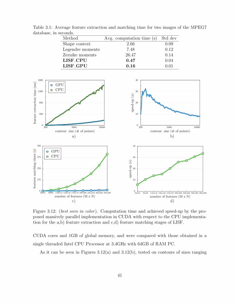
Table 3.1: Average feature extraction and matching time for two images of the MPEG7database, in seconds.
Method Avg. computation time (s) Std devShape context 2.66 0.09Legendre moments 7.48 0.12Zernike moments 26.47 0.14LISF CPU 0.47 0.04LISF GPU 0.16 0.01
featu
re ex
trac
tion tim
e (m
s)
0
400
800
1200
1600
contour size (# of points)200 5000 10000
GPU
CPU
spee
d-u
p (x
)
0
10
20
30
40
contour size (# of points)200 5000 10000
feat
ure
s m
atch
ing
tim
es (s
)
0
125
250
375
500
number of features (M x N)50x50 80x80 110x110 140x140 170x170 200x200 230x230 260x260 290x290
spee
d-u
p (x
)
0
10
20
30
40
number of features (M x N)50x50 80x80 110x110 140x140 170x170 200x200 230x230 260x260 290x290
GPU
CPU
a) b)
c) d)
Figure 3.12: (best seen in color). Computation time and achieved speed-up by the pro-posed massively parallel implementation in CUDA with respect to the CPU implementa-tion for the a,b) feature extraction and c,d) feature matching stages of LISF.
CUDA cores and 1GB of global memory, and were compared with those obtained in a
single threaded Intel CPU Processor at 3.4GHz with 64GB of RAM PC.
As it can be seen in Figures 3.12(a) and 3.12(b), tested on contours of sizes ranging
41
from 200 to 10 000 points, the proposed feature extraction implementation on GPU
achieves up to a 32x speed-up and a 16x average speed-up. The peak in Figure 3.12(b)
represents the point where the used GPU board (approximately at contours of size bigger
than 1000 points), due to its technical specifications, must enqueue the computations that
from the logical programming were determined to be executed in parallel. For the feature
matching step (see Figures 3.12(c) and 3.12(d)), the proposed GPU implementation were
tested comparing from 50 vs. 50 to 290 vs. 290 features. The GPU implementation showed
linear scaling against exponential scaling of the CPU implementation and it obtained a
34x speed-up when comparing 290 vs. 290 LISF features.
3.5 Summary
In this chapter we introduced a method for shape feature extraction, description and
matching, invariant to rotation, translation and scale. The proposed method allows us to
overcome the intrinsic disadvantages of only using local or global features by capturing
both local and global information. The conducted experiments supported the mentioned
contributions, showing larger robustness to partial occlusion than other methods in the
state of the art. It is also more efficient in terms of computational time than the other
techniques. Also, we proposed a massively parallel implementation in CUDA of the two
most time-consuming stages of LISF, i.e., the feature extraction and feature matching
steps, which achieve speed-ups of up to 32x and 34x, respectively. In this chapter we
have presented a shape description and matching method for binary images, in the next
chapter we propose a shape description and matching method for real images (RGB or
grayscale images).
42

Chapter 4
The Open/Closed Contours TriangleArea Representation Method
Shape information have proven to be useful in many image processing and computer
vision applications such as object detection, image retrieval and 3D curve reconstruction.
However, shape representation and matching remains as one of the most challenging topics
in computer vision, partly because of partial occlusion and noise in the shape information
extracted from real images. Figure 4.1 shows a realistic image and the edges extracted
from it using the Pb edge detector (Martin et al., 2004). In edges extracted from real
images, edge fragments that represent part of the object might be missing, e.g., the lower
part of the chair or the left part of the notebook in Figure 4.1 b). Also, contours could
be broken into several fragments. In Figure 4.1 b) we can appreciate that the contours
of the bottle and notebook are broken into several pieces. Furthermore, part of the true
contour of the object of interest can be incorrectly connected to edge fragments belonging
to the background or another object, resulting in a single edge fragment. An example can
be appreciated in Figure 4.1 c), where the bottom of the bottle is connected with edges
from the note and its reflection in the bottle.
Dealing with the three aforementioned problems derived from using edges extracted
from real images implies that the shape descriptor should be able to represent both open
and closed contours, and that part of the contour fragments should match with one or
more parts of the shape model, which makes the shape matching problem more difficult
than that of closed shapes. Other considerations are the robustness with respect to the
43

b) c)a)
Figure 4.1: Problems derived from using edgemaps extracted from real images. a) originalimage, b) edge fragments extracted from a). c) closeup of the bottom part of the bottle.
image scale, rotation and translation.
The LISF method, presented in Chapter 3, is able to deal with partial occlusion, able
to describe open and closed contours, and invariant to scale, rotation and translation
changes. However, LISF cannot perform partial contour matching which is fundamental
when dealing with edgemaps, as above mentioned. Further, LISF description is based
on high curvature contour fragments, ignoring straight line fragments which are in many
cases the primarily structure found in edgemaps obtained from real images.
In this work, we propose a shape descriptor that is particularly suitable for partial
shape matching of open/closed contours extracted from edgemap images, e.g., using
Canny or any other edge extraction method from gray or color images. Our descrip-
tor, named OCTAR (Open/Closed contours Triangle Area Representation), measures the
convexity or concavity of contour segments using the signed areas of triangles formed by
every pair of contour points and their middle point. Based on this descriptor, we also
propose a partial shape matching method robust to partial occlusion and noise in the
extracted contour. The matching method finds for every contour fragment in the query
shape its best match in the shape model. We extend the OCTAR descriptor to represent
44

the spatial configuration of two contour fragments. Individual matches with coherent
spatial configurations with respect to the model are joined to form object hypotheses
in an agglomerative hierarchical process. Later, hypotheses are evaluated based on the
coverage of the model contour, measuring the global shape similarity and its appearance.
4.1 Proposed Shape Descriptor
In order to find partial shape correspondences between contour fragments and a model, a
shape descriptor must be able to represent both open and closed contours, must be self-
contained, and invariant to rotation and translation. In this thesis, we propose a shape
descriptor based on the triangle area representation, that meets these properties. The
proposed descriptor is named OCTAR, from Open/Closed contour Triangle Area Repre-
sentation. The use of triangle areas provides discriminative data about shape features such
as the convexity/concavity at each curve segment. For contour sequences represented in
counter clockwise direction, positive, negative and zero values of OCTAR indicate convex,
concave and straight-line points, respectively.
Given a sequence of N ordered points, P = p1, p2, ..., pN, pi ∈ R2, representing a
contour fragment, for each pair of points 〈pi, pj〉 in P we compute the area of the triangle
formed by these two points and their middle point p∗ ∈ P (see Figure 4.2(a)). The signed
area of the triangle formed by these points is given by Formula 4.1,
TAR(i, j, ∗) =1
2det
xi yi 1x∗ y∗ 1xj yj 1
, (4.1)
where det() is the matrix determinant. If the middle point between 〈pi, pj〉 does not exist,
i.e., (i− j) is odd, p∗ is interpolated from pb(i+j)/2c and pd(i+j)/2e.
To obtain the OCTAR descriptor of contour fragment P , denoted as ΘP , the triangle
area is normalized by the area of the equilateral triangle inscribed in the minimum enclos-
ing circle of the sub-contour pi, ..., pj ⊆ P (it can be proved that this is the maximum
area triangle of all possible triangles inside a circle). In Figure 4.2 (b), the equilateral
normalization triangle is depicted in orange and the minimum enclosing circle of the sub-
45
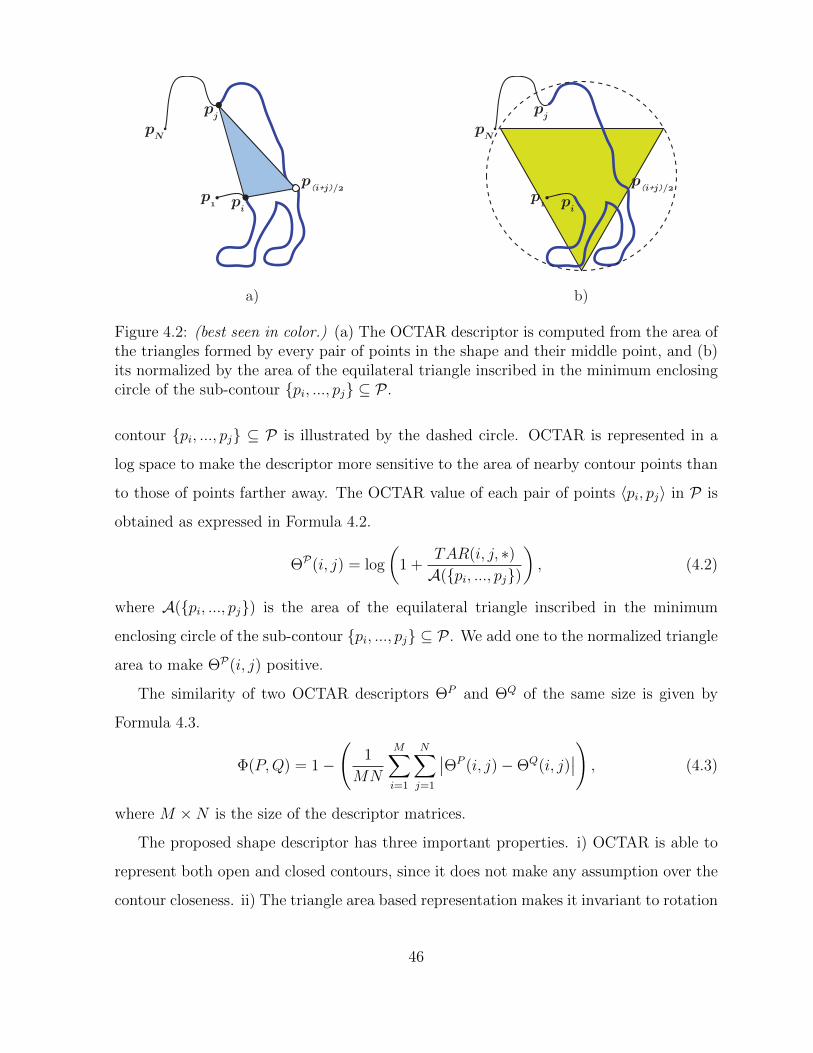
p
pN
pi
pj
p(i+j)/
a) b)
p
pN
pi
pj
p(i+j)/
Figure 4.2: (best seen in color.) (a) The OCTAR descriptor is computed from the area ofthe triangles formed by every pair of points in the shape and their middle point, and (b)its normalized by the area of the equilateral triangle inscribed in the minimum enclosingcircle of the sub-contour pi, ..., pj ⊆ P .
contour pi, ..., pj ⊆ P is illustrated by the dashed circle. OCTAR is represented in a
log space to make the descriptor more sensitive to the area of nearby contour points than
to those of points farther away. The OCTAR value of each pair of points 〈pi, pj〉 in P is
obtained as expressed in Formula 4.2.
ΘP(i, j) = log
(1 +
TAR(i, j, ∗)A(pi, ..., pj)
), (4.2)
where A(pi, ..., pj) is the area of the equilateral triangle inscribed in the minimum
enclosing circle of the sub-contour pi, ..., pj ⊆ P . We add one to the normalized triangle
area to make ΘP(i, j) positive.
The similarity of two OCTAR descriptors ΘP and ΘQ of the same size is given by
Formula 4.3.
Φ(P,Q) = 1−(
1
MN
M∑
i=1
N∑
j=1
∣∣ΘP (i, j)−ΘQ(i, j)∣∣), (4.3)
where M ×N is the size of the descriptor matrices.
The proposed shape descriptor has three important properties. i) OCTAR is able to
represent both open and closed contours, since it does not make any assumption over the
contour closeness. ii) The triangle area based representation makes it invariant to rotation
46

and translation. iii) OCTAR is self-contained as for any C ⊂ P it holds that ΘC ⊂ ΘP ,
this property implicitly allows to retrieve partial matches from the contour description.
Figure 4.3 shows the OCTAR descriptor (Formula 4.2) of two shapes, being the second
shape a subset of the first. As it can be appreciated, the OCTAR descriptor of the second
shape is contained in that of the first shape.
ΘP
PΘC
C
ΘC ⊂ ΘP
⊂P
Figure 4.3: (best seen in color.) The OCTAR descriptor matrices, ΘP and ΘC , of twoshapes, P and C, are shown. The self-containing property of the proposed descriptor canalso be appreciated.
4.2 Proposed Partial Shape Matching Method
Given the set of contour fragments F = f1, f2, ..., fK that represent the query shape
image, where each fragment fk = p1, p2, ..., pNk, pi ∈ R2 is a sequence of Nk points, and
the shape model Q = q1, q2, ..., qM, qi ∈ R2, a sequence of M points; we want to find the
best correspondence between a part fk(a, l) = pa, ..., pa+l−1, fk(a, l) ⊆ fk of a contour
fragment and a part Q(b, l) = qb, ..., qb+l−1,Q(b, l) ⊆ Q of the model, where a and b are
the initial points in fk and Q, respectively, and l is the part length.
Based on the proposed OCTAR descriptor, we introduce a method for finding partial
matches between contour fragments and a model. In order to find partial matches of
arbitrary sizes we have to compare all possible sub-blocks of the descriptor matrices
to find the corresponding sub-blocks with the maximum similarity. With this aim, we
build a 4D tensor T(k, a, b, l) = Φ(fk(a, l),Q(b, l)), where Φ is the similarity measure
47

between descriptor matrices defined in Formula 4.3. To efficiently build T, we use the
integral image optimization to access the partial descriptor differences in constant time,
as suggested in (Riemenschneider et al., 2010). This optimization is possible thanks to
the self-containing property of the OCTAR descriptor.
In order to select the best match between part fk(a, l) ⊆ fk and Q(b, l) ⊆ Q, the
simplest criterion could be to select those fragments with high similarity values in T.
However, given the observation that when very short fragments are involved in a matching,
it is neither discriminative nor reliable, even when having the highest similarity values.
To overcome this limitation, we propose a more robust alternative.
As we want to find which parts of a contour fragment match one or several parts of
the model, we first find which parts of the model are more likely to appear in the contour
fragments. With that aim we suppress the tensor T (k, a, b, l), as indicated in Formula 4.4:
L(k, l, b) =l∑
h=1
Nk∑
a=1
T (k, a, b, h). (4.4)
Given the exhaustive character of T, in a neighborhood of the best matching part
there will be a large amount of strong matches in L. Therefore, we identify the parts of
the model more likely to be involved in a true partial match with one or several parts of
the contour fragment from the shape image as the peaks on L for each length value l,
denoted as Ul = u1, u2, ..., uM, uj ⊆ Q. Figure 4.4 a) represents a contour fragment of
length l from the query image. Its correspondent parts in the swan model are shown in
Figure 4.4 b). The detected peaks in L and their corresponding parts in the model are
shown in Figure 4.4 c).
Once identified the parts of the model that will be involved in a match of length l,
i.e., Ul, we perform the inverse procedure to find which parts of the contour fragment
will match with each identified part in the model. For each part of the model uj ∈ Ul we
suppress the tensor T (k, a, b, l), as indicated in Formula 4.5,
L′(k, l, a) =l∑
h=1
∑
b∈ujT (k, a, b, h), (4.5)
48

a) b) c)
swan model contour
Figure 4.4: (best seen in color). Detection of the parts of the model more likely to beinvolved in a true partial match. In a) a contour fragment of length l from the queryimage, in b) its correspondent parts in the swan model, and in c) the detected peaks inL.
and the peaks in L′ will constitute the matching part of uj in the contour fragment.
Finally, we discard smaller matches contained in another match of larger length value l.
4.3 Object Hypotheses Formation and Evaluation
In presence of partial occlusion and noise, not every contour fragment fk ∈ F has to
be part of the object. Therefore, we have to select among the set of candidate matches
those that really belong to the object. The number of possible combinations of contour
fragments that can be joined to form the object is exponential with respect to the number
of contour fragments. In order to reduce the number of possible combinations, spatial
information is used. Each matched contour fragment is mapped to its corresponding
part in the model and the object centroid estimated. Only matches with neighboring
object centroid estimations can be later joined as an object hypothesis, an example on
the ceazanne image of the EHTZ Shape Classes Dataset in shown in Figure 4.5. Beside
reducing computational time, this step avoids false positives from an early stage.
In order to exploit further the spatial information in an object hypothesis, we extended
the OCTAR shape descriptor, defined in Formula 4.2, such that it could express the spatial
configuration between two contour fragments P = p1, p2, ..., pN and R = r1, r2, ..., rM,where each point pi ∈ P is related with each point rj ∈ R through the area of the triangle
49

Figure 4.5: (best seen in color). Partial matches that according to their spatial relationscan be later joined as an object hypothesis (connected by a yellow edge).
formed by pi, rj, and the first point in R (see Figure 4.6). The spatial configuration
descriptor of two contour fragments P and R is defined as
ΘP,R(pi, rj) = log
(1 +
TAR(pi, rj, r1)
A(pi, rj, r1)
), (4.6)
where TAR(pi, rj, r1) is the signed area (see Formula 4.1) of the triangle formed by the
first point of the contour fragment R and the ith and jth points of the contour fragments
P and R, respectively. A(pi, rj, r1) is the area of the equilateral triangle inscribed in
the minimum enclosing circle of the point set pi, rj, r1.
pi
P R
pi
PR
ΘP,R ΘP ,R
Figure 4.6: (best seen in color). Extended OCTAR descriptor for contours spatial con-figuration. The same two contours under different spatial configurations have differentdescriptor matrices.
In order to form object hypotheses, we use an agglomerative hierarchical approach
in the spatial configuration space. Initially, each match is a hypothesis; later, in each
iteration, the two hypotheses whose contour fragments configuration is more similar to
its corresponding configuration of model parts are joined, restricted to those fragments
with neighboring object centroid estimations.
50

Once the hypotheses hierarchy is obtained, each object hypothesis is evaluated accord-
ing to four criteria. These criteria evaluate in what extent the object model is covered, the
hypothesis global shape similarity with respect to the model, and its appearance. These
hypothesis evaluation criteria are detailed in the following sections.
4.3.1 Covering Criterion
The first criterion is based on the coverage of the model contour by the hypothesis, and
is defined as indicated in Expression 4.7.
ECOV =1
M
M∑
i
wi, (4.7)
where wi takes value of one or zero to indicate whether the ith point of the model contour
has been matched or not, and M is the number of points in the model contour.
4.3.2 Object Hypothesis Contour Estimation Criterion
The second hypothesis evaluation measure assesses the shape similarity in a global man-
ner. An object hypothesis is a set of partial matches, therefore it is expressed as the
correspondence between a subset of contour fragment points in the image and a subset of
points in the model. The idea is to estimate the whole contour of the object hypothesis
in the image based on the existing correspondences.
There is a mapping T : Q → F , such that if p ∈ Q, T (p) ∈ F . The subset of points in
the object hypothesis in the image is denoted as F ∈ F and the corresponding subset of
points in the model is denoted as Q ∈ Q. Usually, in an object hypothesis, there are some
points in the model that have no correspondence in the image, i.e., Q = p ∈ Q|p /∈ Q.For each point p ∈ Q, we estimate its correspondent point in the image based on a
transformation Z, consisting on rotation and translation, which is estimated locally based
on the correspondences between F and Q. Therefore, the whole object hypothesis contour
in the image is expressed as indicated in Formula 4.8.
H(p) =
T (p), if p ∈ QpZp, if p ∈ Q (4.8)
51

We estimate the transformation Zp for each point p ∈ Q, as the rotation and transla-
tion transformation between a neighborhood Vp ∈ Q of point p and their correspondent
points T (Vp) in the image. The neighborhood Vp of point p in Q is defined as the closest
points of p in the contour sequence, i.e., the distance is stablished over the model contour
indexes.
The transformation Zp is computed using the Iterative Closest Point (ICP) algorithm
(Besl and McKay, 1992; Chen and Medioni, 1992). The ICP algorithm aims to find
the transformation between a point cloud and some another reference point cloud, by
minimizing the squared errors between the corresponding points.
Finally, we evaluate each object hypothesis based on the OCTAR similarity score
(Formula 4.3) between the whole object hypothesis contour in the image H and the
model Q:
EZ = Φ(H,Q). (4.9)
4.3.3 Fitted Object Hypothesis Criterion
Evaluating if the estimated object hypothesis contour H is consistent with the edge frag-
ments in the image is also needed. With this purpose, we fit every point p ∈ H to its
nearest point in the edge image F , as expressed in Formula 4.10,
H∗(p) =
p, if p ∈ F
NN(p) ∈ F , if p /∈ F (4.10)
To find the nearest point of p in F we use the kd-tree algorithm. Later, each hypothesis
evaluation is given by the OCTAR similarity between the estimated object contour and
this same contour fitted to the image edges, as indicated in Formula 4.11.
EZ∗ = Φ(H,H∗). (4.11)
52

4.3.4 Appearance-based Evaluation Criterion
As mentioned in Sections 1.1 and 2.3, appearance features may provide distinctive cues
for the object recognition process. In our work, we use appearance information in the
same way as (Biederman and Ju, 1988) suggested. In this work authors argue that
appearance information is used by humans to recognize objects as a second-level feature.
For appearance representation we use a BoW-based representation.
In order to build the visual vocabulary, positive samples for each class are taken from
the ground-truth bounding boxes on the training set. The bounding boxes are resized to a
reference size while keeping its aspect ratio. SIFT descriptors (Lowe, 2004) are computed
over circular patches of radius M , at points on a regular grid with spacing also M pixels.
From the dense features a visual vocabulary is obtained. For more details about the BoW
representation used see Chapter 5, which presents our proposal on how to obtain a more
discriminative, representative and compact BoW representation. Later, from the training
set, we use Support Vector Machine (SVM) to learn a classifier.
For evaluating each object hypothesis, its bounding box is resized to the reference
size, and the SIFT descriptors extracted over circular patches on a grid in the same way
as it was explained above for the case of the training images. The object hypothesis is
represented using the previously obtained vocabulary and then we measure its relevance
to a class, using the confidence of the learned SVM model, denoted as EApp.Finally, we select as final match the hypothesis with the largest linear combination of
ECOV , EZ , EZ∗ and EApp, defined as expressed in Formula 4.12,
M∗ = arg max [αECOV + βEZ + γEZ∗ + δEApp] , (4.12)
where α, β, γ and δ are the weights associated to ECOV , EZ , EZ∗ and EApp, respectively.
In all our experiments we used α = β = γ = δ = 1 to equally favor the four criteria.
53

4.4 Experimental Results
4.4.1 Performance Evaluation on Real Scenes
We present results on the ETHZ Shape Classes Dataset (Ferrari et al., 2006). This dataset
contains images of five diverse shape-based classes: Apple logos, bottles, giraffes, mugs
and swans, and contains a total of 255 images. Example images for each category could
be seen in Figure 4.7. The ETHZ Shape Classes Dataset is highly challenging as there is
considerable intra-class shape variation, the objects appear in a wide range of scales and
many images are severely cluttered, with objects comprising only a fraction of the total
image area. Most images contain a single instance of an object class, while some contain
multiple instances. No image contains instances of different classes. Object ground-truth
bounding boxes and object outlines are included. Also, edgemaps produced by the Pb
edge detector (Martin et al., 2004) are provided. Figure 4.8 shows the edgemaps of the
ETHZ dataset examples images presented in Figure 4.7.
Figure 4.7: (best seen in color.) Example images from the ETHZ Shape Classes dataset.From left to right the Apple logo, bottle, giraffe, mug and swan class.
54

Figure 4.8: (best seen in color.) Example edgemap images from the ETHZ Shape Classesdataset. From left to right the Apple logo, bottle, giraffe, mug and swan class.
For the purpose of object detection evaluation we follow the protocol in (Ferrari et al.,
2010). We use the provided single hand-drawing shape models as the reference shape
model Q for its corresponding class. We use the first half of images in each class for
training the object appearance and the second half for testing. For evaluation, we use the
PASCAL Challenge criterion, i.e., a detection is counted as correct only if the intersection-
over-union ratio with the ground-truth bounding box is greater than 50%, otherwise
detections are counted as false-positives.
Table 4.1 shows the interpolated average precision (AP) in the ETHZ dataset and a
comparison with several state-of-the-art shape-based methods. Our method obtained the
best AP for the Giraffes class, given that Giraffes are highly textured objects we suspect
that the use of appearance cues played an important role. Our AP is comparable with
the other methods in the rest of the classes. Our mean average precision over the five
classes is comparable with the best results. We also present results of our method without
the appearance evaluation criterion (OCTAR - EApp), in order to show the improvement
55
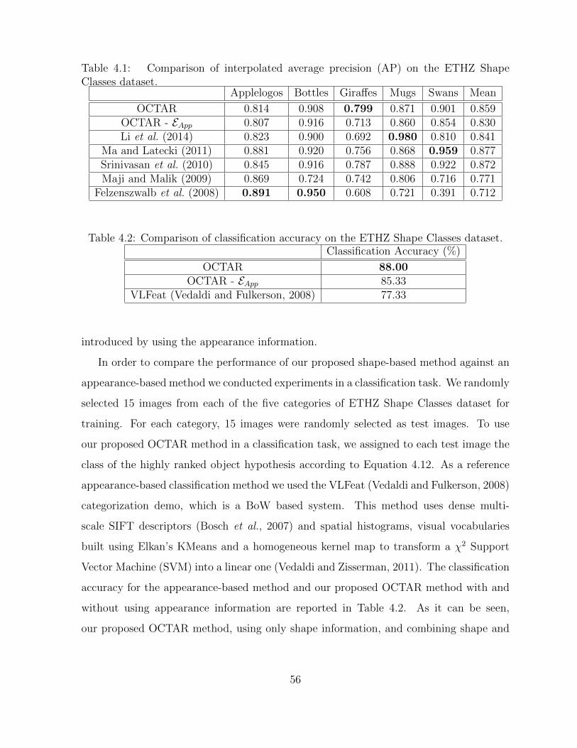
Table 4.1: Comparison of interpolated average precision (AP) on the ETHZ ShapeClasses dataset.
Applelogos Bottles Giraffes Mugs Swans Mean
OCTAR 0.814 0.908 0.799 0.871 0.901 0.859OCTAR - EApp 0.807 0.916 0.713 0.860 0.854 0.830Li et al. (2014) 0.823 0.900 0.692 0.980 0.810 0.841
Ma and Latecki (2011) 0.881 0.920 0.756 0.868 0.959 0.877Srinivasan et al. (2010) 0.845 0.916 0.787 0.888 0.922 0.872Maji and Malik (2009) 0.869 0.724 0.742 0.806 0.716 0.771
Felzenszwalb et al. (2008) 0.891 0.950 0.608 0.721 0.391 0.712
Table 4.2: Comparison of classification accuracy on the ETHZ Shape Classes dataset.Classification Accuracy (%)
OCTAR 88.00OCTAR - EApp 85.33
VLFeat (Vedaldi and Fulkerson, 2008) 77.33
introduced by using the appearance information.
In order to compare the performance of our proposed shape-based method against an
appearance-based method we conducted experiments in a classification task. We randomly
selected 15 images from each of the five categories of ETHZ Shape Classes dataset for
training. For each category, 15 images were randomly selected as test images. To use
our proposed OCTAR method in a classification task, we assigned to each test image the
class of the highly ranked object hypothesis according to Equation 4.12. As a reference
appearance-based classification method we used the VLFeat (Vedaldi and Fulkerson, 2008)
categorization demo, which is a BoW based system. This method uses dense multi-
scale SIFT descriptors (Bosch et al., 2007) and spatial histograms, visual vocabularies
built using Elkan’s KMeans and a homogeneous kernel map to transform a χ2 Support
Vector Machine (SVM) into a linear one (Vedaldi and Zisserman, 2011). The classification
accuracy for the appearance-based method and our proposed OCTAR method with and
without using appearance information are reported in Table 4.2. As it can be seen,
our proposed OCTAR method, using only shape information, and combining shape and
56

appearance, outperformed the appearance-based method in this experiment.
4.4.2 Performance Evaluation on Occluded Shapes
In order to obtain a more clear evaluation of the robustness of the proposed OCTAR
method to partial occlusion and missing edges, we performed a second set of experiments
over artificially occluded shapes. The experiments were conducted on two different well-
known datasets. The first dataset is the Kimia Shapes99 dataset (Sebastian et al., 2004),
which includes 9 categories and 11 shapes in each category with variations in form, occlu-
sion, articulation and missing parts. The second dataset is the Kimia Shapes216 dataset
(Sebastian et al., 2004). The Shapes216 database consists of 18 categories with 12 shapes
in each category. In the two datasets, in each image there is only one object, defined by
its silhouette, and at different scales, rotations and positions.
In order to show the robustness of the proposed method to partial occlusion, we
generated another 14 datasets by artificially introducing occlusion of different magnitudes
(10%, 20%,...,70%) to the Shapes99 and Shapes216 datasets. Occlusion was added by
randomly removing 2 to 5 fragments of the entire contour, whose total length represents
the desired partial occlusion. A sample image from the Shapes216 dataset at different
occlusion levels is shown in Figure 4.9.
0% 10% 20% 30% 40% 50% 60% 70%
Figure 4.9: Example image from the Shapes216 dataset with different levels of occlusion(0%, 10%, 20%, 30%, 45% and 60%) used in the experiments.
As a measure to evaluate and compare the performance of the proposed shape matching
schema in a shape retrieval scenario we use the so-called bull’s eye score. Each shape in
the database is compared with every other shape model, and the number of shapes of the
same class that are among the 2Nc most similar is reported, where Nc is the number of
instances per class. The bull’s eye score is the ratio between the total number of shapes
57

of the same class and the largest possible value. The results obtained by our proposed
method were compared with those of the popular shape context (Belongie et al., 2002)
and IDSC (Ling and Jacobs, 2007) descriptors. Figure 4.10 shows the behavior of the
bull’s eye score of each method.
OCTAR vs.
a) b) c)
Shapes99 dataset
OCTAR
Shape contextIDSC
bullse
ye sc
ore
(%)
20
40
60
80
100
partial occlusion (%)0 10 20 30 40 50 60 70
OCTAR
Shape contextIDSC
bullse
ye sc
ore
(%)
10
32.5
55
77.5
100
partial occlusion (%)0 10 20 30 40 50 60 70
Shapes216 dataset
bullse
ye
scor
e diffe
rence
(%)
-5
10
25
40
55
partial occlusion (%)0 10 20 30 40 50 60 70
SC-Shapes99
IDSC-Shapes216
IDSC-Shapes99
SC-Shapes216
Figure 4.10: (best seen in color). Bull’s eye score comparison between OCTAR, shapecontext and IDSC in the a) Shapes99 and b) Shapes216 datasets with different partialocclusions. In c) the OCTAR improvement compared to shape context and IDSC.
As expected, our proposed method outperformed the shape context and IDSC meth-
ods. Moreover, while increasing the occlusion level, the difference in terms of bull’s eye
score gets bigger, with about 30 - 50% higher bull’s eye score across highly occluded im-
ages (see Figure 4.10(c)); which shows the advantages of OCTAR over the other two, in
particular for highly occluded contours. The computation time of our proposed method
has been also evaluated and compared against other methods. Table 4.3 shows the aver-
age time taken by OCTAR, shape context and IDSC for extracting and matching features
of two shapes. These results were obtained on a single thread of a 2.2 GHz CPU and
8GB RAM PC. As it can be seen, OCTAR is faster than shape context and comparable
to IDSC.
4.5 Summary
As a result of this work, a shape descriptor for open and closed contours, and a partial
shape matching method have been proposed. The proposed descriptor and matching
method allow us to find the best matching parts of a query object with a model in presence
58

Table 4.3: OCTAR average feature extraction and matching time for two images of theMPEG7 database, in milliseconds.
Method Avg. computation time (ms) Std devShape context 1710 40.9IDSC 6 0.1OCTAR (our method) 45 3.2
of partial occlusion and noise. Also, the proposed method is invariant to rotation and
translation. Unlike the LISF method, presented in Chapter 3, the OCTAR method is
able to detect and recognize objects in complex real world images, as it is capable to
deal with the intrinsic problems derived from using edgemaps obtained from real images.
The OCTAR method allowed to evaluate object detection hypotheses according to several
criteria, including the evaluation of the hypothesis appearance. In the next Chapter we
present our proposed appearance-based representation method, which selects the most
discriminative and representative visual words on a BoW-based representation.
59

Chapter 5
Improving Visual Vocabularies
Appearance-based features have proved to play an important role in object recognition.
In our proposed method, OCTAR, presented in Chapter 4, we combined shape and ap-
pearance features for category-level object recognition, specifically by using appearance
as a second level feature. In this Chapter we introduce our BoW-based appearance rep-
resentation, which selects the most representative and discriminative visual words from a
given visual vocabulary.
One of the most widely used approaches for representing images for object catego-
rization is the Bag of Visual Words (BoW) approach (Csurka et al., 2004). BoW-based
methods have obtained remarkable results in recent years and they even obtained the
best results for several classes in the recent PASCAL Visual Object Classes Challenge
on object classification (Everingham et al., 2011). The key idea of BoW approaches is
to discretize the entire space of local features (e.g., SIFT (Lowe, 2004)) extracted from a
training set at interest points or densely sampled in the image. With this aim, clustering
is performed over the set of features extracted from the training set in order to identify
features that are visually equivalent. Each cluster is interpreted as a visual word, and
all clusters form a so-called visual vocabulary. Later, in order to represent an unseen
image, each feature extracted from the image is assigned to a visual word of the visual
vocabulary; from which a histogram of occurrences of each visual word in the image is
obtained, as illustrated in Figure 5.1.
One of the main limitations of the BoW approach is that the visual vocabulary is built
60

1.) Local Feature Extraction
2.) Feature Description
3.) Visual Vocabulary
) Ranking and Filtering
4.) Bag of Words
1. k52. k23. k44. k1
1. k52. k23. k44. k1
5. k66. k3
.
.
.
.
.
.
.
.
.
.
.
.
.
.
.
.
.
.
.
.
.
.
.
.
*
FilteringRanking
k1
k2
k3
k4
k5
k6k1 k2 kK. . .
k1 k2 kK. . .
k1 k2 kK. . .
k1 k2 kK. . .
Figure 5.1: Classical BoW approach overview (steps 1 to 4). First, regions/points ofinterest are automatically detected and local descriptors over those regions/points arecomputed (step 1 and 2). Later in step 3, the descriptors are quantized into visual wordsto form the visual vocabulary. Finally, in step 4, the occurrences in the image of eachspecific word in the vocabulary for constructing the BoW feature are found. In thischapter, we propose to introduce step (∗) in order to use only the most discriminativeand representative visual words from the visual vocabulary in the BoW representation.
using features that belong to both the object and the background. This implies that the
noise extracted from the image background is also considered as part of the object class
description. Also, in the BoW representation, every visual word is used, regardless of
its low representativeness or discriminative power. These elements may limit the quality
of further classification processes. In addition, there is no consensus about which is the
optimal way for building the visual vocabulary, i.e., the clustering algorithm used, the
number of clusters (visual words) that best describe the object classes, etc. When dealing
with relatively small vocabularies, clustering can be executed several times and the best
performing vocabulary can be selected through a validation phase. However, this becomes
intractable for large image collections.
In this chapter, we propose three properties to assess the ability of a visual word
to represent and discriminate an object class in the context of the BoW approach. We
define three measures in order to quantitatively evaluate each of these properties. The
visual words that best represent a class, best generalize over intra-class variability and
best differentiate between object classes will obtain the highest scores for these measures.
A methodology for reducing the size of the visual vocabulary based on these properties is
61

also proposed. Our proposal does not depend on the clustering method used to create the
visual vocabulary, the descriptor used (e.g., SIFT, SURF, etc.) or the weighting scheme
used (e.g., tf, tf-idf, etc.). Therefore, it can be applied to a previously built vocabulary to
improve its representativeness, since it does not build a new visual vocabulary, it rather
finds the best visual words of a given visual vocabulary.
Experiments conducted on the Caltech-101 (Fei-Fei et al., 2007) and Pascal VOC 2006
(Everingham et al., 2006) datasets, in a classification task, demonstrate the improvement
introduced by the proposed method. Tested with different vocabulary sizes, different in-
terest points extraction and description methods, and different weighting schemas, the
classification accuracies achieved using the entire vocabulary were always statistically in-
ferior to those achieved by several of the vocabularies obtained by filtering the baseline
vocabulary, using our proposed vocabulary size reducing methodology. Moreover, the
best results were obtained with as few as the 13.4% and 34.5%, in average, of the baseline
visual words for the Caltech-101 and Pascal VOC 2006 datasets, respectively. Compared
with a state-of-the-art mutual information based method for feature selection our pro-
posal obtains superior classification accuracy results for the highest compression rates
and comparable results for the other filtering sizes.
5.1 Proposed Method
Visual vocabularies are commonly comprised by a lot of noisy visual words due to intra-
class variability and the inclusion of features from the background during the vocabulary
building process, among others. Later, for image representation every visual word is used,
which may lead to an error-prone image representation.
In order to improve image representations, we introduce three properties and their
corresponding quantitative evaluations to assess the ability of a visual word to represent
and discriminate an object class in the context of the BoW approach. We also propose
a methodology, based on these properties, for reducing the size of the visual vocabulary,
discarding those visual words that worst describe an object class (i.e., noisy visual words).
62

Reducing the vocabulary in such a manner will allow to have a more reliable and compact
image representation.
We would like to emphasize that all the measures proposed in this section are used
during the training phase; therefore, we can use all the knowledge about the data that is
available during this phase.
5.1.1 Inter-class Representativeness Measure
A visual word could be comprised of features from different object classes, representing
visual concepts or parts of objects common to those different classes. These common
parts or concepts do not have necessarily to be equally represented inside the visual word
because, even when similar, object classes should also have attributes that differentiate
them. Therefore, we can say that, in order to best represent an object class, a property
that a visual word must satisfy is to have a high representativeness of this class. In
order to measure the representativeness of a class cj in visual word k, theM1 measure is
proposed as expressed in Formula 5.1.
M1(k, cj) =fk,cjnk
, (5.1)
where nk is the total number of features in visual word k and fk,cj represents the number
of features of class cj in visual word k, i.e., the number of visual descriptors of class cj
that belong to the cluster corresponded to visual word k.
Figure 5.2 shows M1 values for two example visual words. In Figure 5.2 a) the circle
class has a very high value ofM1 because most of the features in the visual word belong
to the circle class, being the opposite for the classes square and triangle that are poorly
represented in the visual word. Figure 5.2 b) shows an example visual word where every
class is nearly equally represented, therefore every class has similar M1 values.
5.1.2 Intra-class Representativeness Measure
A visual word could be comprised of features from different objects, many of them prob-
ably belonging to the same object class. Even when different, object instances from the
63
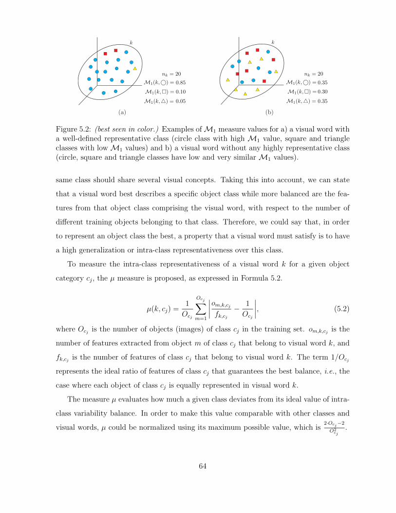
(a) (b)
k k
nk = 20
M1(k, ) =
M1(k, ) =
M1(k, ) =
0.85
0.10
0.05
nk = 20
0.35
0.30
0.35
M1(k, ) =
M1(k, ) =
M1(k, ) =
Figure 5.2: (best seen in color.) Examples ofM1 measure values for a) a visual word witha well-defined representative class (circle class with high M1 value, square and triangleclasses with lowM1 values) and b) a visual word without any highly representative class(circle, square and triangle classes have low and very similar M1 values).
same class should share several visual concepts. Taking this into account, we can state
that a visual word best describes a specific object class while more balanced are the fea-
tures from that object class comprising the visual word, with respect to the number of
different training objects belonging to that class. Therefore, we could say that, in order
to represent an object class the best, a property that a visual word must satisfy is to have
a high generalization or intra-class representativeness over this class.
To measure the intra-class representativeness of a visual word k for a given object
category cj, the µ measure is proposed, as expressed in Formula 5.2.
µ(k, cj) =1
Ocj
Ocj∑
m=1
∣∣∣∣om,k,cjfk,cj
− 1
Ocj
∣∣∣∣, (5.2)
where Ocj is the number of objects (images) of class cj in the training set. om,k,cj is the
number of features extracted from object m of class cj that belong to visual word k, and
fk,cj is the number of features of class cj that belong to visual word k. The term 1/Ocj
represents the ideal ratio of features of class cj that guarantees the best balance, i.e., the
case where each object of class cj is equally represented in visual word k.
The measure µ evaluates how much a given class deviates from its ideal value of intra-
class variability balance. In order to make this value comparable with other classes and
visual words, µ could be normalized using its maximum possible value, which is2·Ocj−2
O2cj
.
64

(a) (b)
k k
O = 4
fk, = 17
M2(k, ) = 0.9559
o‘red’,k, = 5
o‘blue’,k, = 4
o‘yellow’,k, = 4
o‘gray’,k, = 4
O = 4
fk, = 17
M2(k, ) = 0.4853
o‘red’,k, = 1
o‘blue’,k, = 13
o‘yellow’,k, = 1
o‘gray’,k, = 2
Figure 5.3: (best seen in color.) Examples ofM2 measure values for the circle class in a)a visual word where there is a good balance between the number of features of differentimages of the circle class (high M2 value), and in b) the opposite case where only oneimage for the circle class is predominantly represented in the visual word (lowM2 value).In the figure, different fill colors of each feature in the visual word represent featuresextracted from different object images of the same class.
Taking into account that µ takes its maximum value in the worst case of intra-class
representativeness, the measure M2 is defined to take its maximum value in the case of
ideal intra-class variability balance and to be normalized by max(µ(k, cj)):
M2(k, cj) = 1− Ocj
2 · (Ocj − 1)
Ocj∑
m=1
∣∣∣∣om,k,cjsk,cj
− 1
Ocj
∣∣∣∣. (5.3)
Figure 5.3 shows the values ofM2 on two example visual words. In Figure 5.3 a), the
number of features from the different images of the circle class in the visual word is well
balanced, i.e., the visual word generalizes well over intra-class variability for the circle
class, hence this class presents a high M2 value. In contrast, in Figure 5.3 b) only one
image from the circle class is well represented by the visual word. As the visual word
represents a visual characteristic only present in one image, it is not able to well represent
intra-class variability, therefore, the circle class will have a low value ofM2 in this visual
word.
65

5.1.3 Inter-class Distinctiveness Measure
M1 andM2 provide, under different perspectives, a quantitative evaluation of the ability
of a visual word to describe a given class. However, we should not build a vocabulary just
by selecting those visual words that best represent each object class, because this fact
does not directly imply that the more representative words will be able to differentiate
well one class from another, as a visual vocabulary is expected to do. Therefore, we can
state that, in order to be used as part of a visual vocabulary, a desired property of a visual
word is that it should have high values of M1(k, cj) and M2(k, cj) (represents well the
object class), while having low values of M1(k, cjC) and M2(k, cjC) (misrepresents
the rest of the classes), i.e., it must have high discriminative power.
In order to quantify the distinctiveness of a visual word for a given class, the measure
M3 is proposed. M3 expresses how much the object class that is best represented by
visual word k is separated from the other classes in the M1 and M2 rankings.
Let ΘM(K, cj) be the set of values of a given measureM for the set of visual wordsK =
k1, k2, ..., kN and the object class cj, sorted in descending order of the value ofM. Let
Φ(k, cj) be the position of visual word k ∈ K in ΘM(K, cj). Let Pk = mincj∈C(Φ(k, cj))
be the best position of visual word k in the set of all object classes C = c1, c2, ..., cQ.Let ck = arg mincj∈C(Φ(k, cj)) be the object class where k has position Pk. Then, the
inter-class distinctiveness (measureM3), of a given visual word k for a given measureM,
is defined as expressed in Formula 5.4.
M3(k,M) =1
(|C| − 1)(|K| − 1)
C∑
cj 6=ck(Φ(k, cj)− Pk). (5.4)
In Figure 5.4, the M3 measure is calculated for two visual words (i.e., k2 and k5) of
a six visual words and three classes example. Visual word k2 is among the top items of
the representativeness ranking for every class in the example. Despite this, k2 has low
discriminative power because describing well several classes makes harder the process of
differentiate one class from another. In contrast, visual word k5 is highly discriminative
because it describes well only one class.
66

ΘM(K, c1) ΘM(K, c2) ΘM(K, c3)
1. k2 k2 k1
2. k1 k5 k2
3. k3 k4 k4
4. k4 k6 k6
5. k6 k1 k5
6. k5 k3 k3
Ran
kin
g pos
itio
n
Pk2 = 1, ck2 = 1
0.1
M3(k2,M) = 1(|C|−1)(|K|−1)
∑Ccj 6=ck2
(Φ(k2, cj) − Pk2)
M3(k2,M) =
Pk5 = 2, ck5 = 2
0.7
M3(k5,M) = 1(|C|−1)(|K|−1)
∑Ccj 6=ck5
(Φ(k5, cj) − Pk5)
M3(k5,M) =
Figure 5.4: (best seen in color.) Example of M3 measure for two visual words. k2 haslow discriminative power because it represents well several classes, while k5 has highdiscriminative power because it describes well only one class.
5.1.4 On Ranking and Reducing the Size of Visual Vocabularies
The proposed measures provide a quantitative evaluation of the representativeness and
distinctiveness of the visual words in a vocabulary for each class. The visual words that
best represent a class, best generalize over intra-class variability and best differentiate
between object classes, will obtain the highest scores for these measures. In this section,
we present a methodology for ranking and reducing the size of the visual vocabularies,
towards more reliable and compact image representations.
Let ΘM1(K) and ΘM2(K) be the rankings of vocabulary K, using measures
M3(K,M1) and M3(K,M2), respectively. ΘM1(K) and ΘM2(K) provide a ranking
of the vocabulary based on the distinctiveness of visual words according to inter-class and
intra-class variability, respectively.
In order to find a consensus, Θ(K), between both rankings ΘM1(K) and ΘM2(K) a
consensus-based voting method can be used; in our case, we decided to use the Borda
Count algorithm (Emerson, 2013) although any other can be used as well. The Borda
Count algorithm obtains a final ranking from multiple rankings over the same set. Given
|K| visual words, a visual word receives |K| points for a first preference, |K| − 1 points
for a second preference, |K| − 2 for a third, and so on for each ranking independently.
Later, individual values for each visual word are added and a final ranking obtained.
67

From this final ranking a reduced vocabulary can be obtained by selecting the first N
visual words. As pointed in (Liu and Shah, 2008), the size of the vocabulary affects the
performance and there is a vocabulary size which can achieve maximal accuracy, which
depends on the dataset, the number of classes and the data nature, among others. In our
experiments, we explore different vocabulary sizes, over different datasets, different inter-
est points extraction and description methods, different weighting schemas, and different
classifiers.
5.2 Experimental Evaluation
In this chapter we have presented a methodology for improving BoW-based image rep-
resentation by using only the most representative and discriminative visual words in the
vocabulary. As it was stated in previous sections, our proposal does not depend on the
algorithm used for building the set of visual words, the descriptor used nor the weighting
scheme used. Therefore, the proposed methodology could be applied for improving the
accuracy of any of the methods reported in the literature, which are based on a BoW
approach.
The main goal of the experiments we present in this section is to quantitatively evalu-
ate the improvement introduced by our proposal to the BoW-based image representation,
over two standard datasets commonly used in object categorization. The experiments
were focused on: a) to assess the validity of our proposal in a classic BoW-based classifi-
cation task, b) to evaluate the methodology directly with respect to other kinds of feature
selection algorithms in the state of the art, and c) to measure the time our methodology
spent in order to filter the visual vocabulary built for each dataset. All the experiments
were done on a single thread of a 3.6 GHz Intel i7 processor and 64GB RAM PC.
The experiments conducted in order to evaluate our proposal were done in two well-
known datasets: Caltech-101 (Fei-Fei et al., 2007) and Pascal VOC 2006 (Everingham
et al., 2006).
The Caltech-101 dataset (Fei-Fei et al., 2007) consists of 102 object categories. There
68

are about 40 to 800 images per category and most categories have about 50 images. The
Pascal VOC 2006 dataset (Everingham et al., 2006) consists of 10 object categories. In
total, there are 5304 images, split into 50% for training/validation and 50% for test-
ing. The distributions of images and objects by class are approximately equal across the
training/validation and test sets.
5.2.1 Assessing the Validity in a Classic BoW-based Classifica-tion Task
As it was mentioned before, the goal of the first experiment is to assess the validity of our
proposal. With this aim, we evaluate the accuracy in a classic BoW-based classification
task, with and without applying our vocabulary filtering methodology.
In the experiments presented here, we use for image representation the BoW schema
presented in Figure 5.1 with the following specifications:
• Interest points are detected and described using two methods: SIFT (Lowe, 2004)
and SURF (Bay et al., 2008).
• K-means, with four different K values, is used to build the visual vocabularies; these
vocabularies constitute the baseline. For Caltech-101 dataset we used K=10000,
15000, 20000 and 25000, while for Pascal VOC 2006 dataset we used K=200, 1000,
5000 and 10000.
• Each of the baseline vocabularies is ranked using our proposed visual words ranking
methodology.
• Later, nine new vocabularies are obtained by filtering each baseline vocabulary,
leaving the 10%, 20%, ..., 90%, respectively, of the most representative and discrim-
inative visual words based on the obtained ranking.
• Two weighting schemas are used for image representation: tf and tf-idf.
• For both datasets we randomly selected 10 images from all the categories for building
the visual vocabularies. The rest of the images were used as test images; but, as in
69

(Lazebnik et al., 2006), we limited to 50 the number of test images per category.
After that, we tested the obtained visual vocabularies in a classification task, using
SVM (with a linear kernel) and KNN (where K is optimized with respect to the leave-one-
out error) as classifiers. For each visual vocabulary, test images are represented using this
vocabulary and, a 10-fold 10-times cross-validation process is conducted, where nine of
the ten partitions are used for training and the other one for testing the trained classifier.
The mean classification accuracy along the ten iterations is reported.
Figures 5.5 and 5.6 show the mean classification accuracy results over the cross-
validation process using SVM and KNN, respectively, on the Caltech-101 dataset. Figures
5.7 and 5.8 show the same for the Pascal VOC 2006 dataset. In Figures 5.5 to 5.8, sub-
figures (a) and (b) show the results using SIFT descriptor; results for SURF are shown in
subfigures (c) and (d). Results for the two different weighting schemas, i.e., tf and tf-idf,
are shown in subfigures (a) (c), and (b) (d), respectively.
It can be seen that in both datasets, for every configuration, our proposed methodology
allows to obtain reduced vocabularies that outperformed the classical BoW approach
(baseline).
Table 5.1 summarizes the results presented in Figures 5.5 and 5.6 for the Caltech-
101 dataset. The results in Figures 5.7 and 5.8 are summarized in Table 5.2. For every
experiment configuration, Tables 5.1 and 5.2 show the baseline classification accuracy
against the best result obtained by the proposed method with both SVM and KNN
classifiers. The size of the filtered vocabulary in which the best result was obtained is also
showed.
Discussion
The experimental results presented in this section validate the claimed contributions of our
proposed method. As it can be seen in Tables 5.1 and 5.2, the best results obtained with
our proposed method outperform those obtained with the whole vocabularies. For the
experiments conducted in the Caltech-101 dataset, our average best results outperformed
the baseline by a 4.6% and 4.8% in mean classification accuracy using SVM and KNN,
70
respectively. In the Pascal VOC 2006 dataset there was a 3.2% and 7% improvement
for SVM and KNN, respectively. As noticed on Figures 5.5 to 5.8, the trend of the
performance with respect to the filter size is not the same in the two considered datasets.
In the Caltech-101 dataset, for smaller filter sizes higher accuracies, while in the Pascal
VOC 2006 dataset a so well defined trend was not noticed. We suspect that the Pascal
VOC 2006 dataset does not present a definite trend due to its specific characteristics,
i.e., a fewer number of classes, fewer number of training images and smaller sizes initial
vocabularies. Nonetheless, despite not having a definite trend, and as mentioned before,
the reduced vocabularies mostly obtained better classification accuracy than the entire
vocabulary in the Pascal VOC 2006 dataset.
In order to validate the improvement obtained by the proposed method, the statistical
significance of the obtained results was verified. For testing the statistical significance
we used the Mann-Whitney test (Mann and Whitney, 1947), with a 95% of confidence.
Appendix A presents the detailed explanation of this test. An implementation of the test
can be found in (vas, 2013). As a result of the Mann-Whitney test, it has been verified that
the results obtained in both datasets, by the proposed method, are statistically superior
to those obtained by the baseline.
In addition, the best results using the filtered vocabularies were obtained with vocab-
ularies several times smaller than the baseline vocabularies, i.e., 6 and 10 times smaller
in average using SVM and KNN, respectively, for the Caltech-101 datasets, and 2 and
5 times smaller in average for the Pascal VOC 2006 dataset with SVM and KNN, re-
spectively. Furthermore, vocabularies 10 times smaller always obtained better accuracy
results than the baseline vocabularies in the Caltech-101 dataset, and in the 78.1% of
the experiments on the Pascal VOC 2006 dataset. Obtaining smaller vocabularies implies
more compact image representations, that will have a direct impact on the efficiency of
further processing based on these image representations, and less memory usage.
Also, the conducted experiments provide evidence that a large number of visual words
in a vocabulary are noisy or little discriminative. Discarding these visual words allows for
a better and more compact image representation.
71
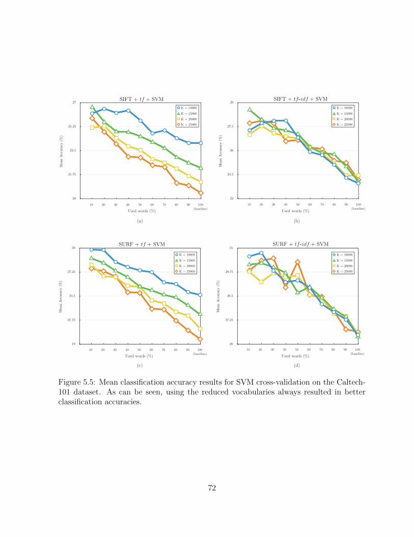
(a) (b)
SIFT + tf + SVM
Mea
n A
ccura
cy (
%)
10 20 30 40 50 60 70 80 90 100(baseline)
SIFT + tf-idf + SVM
Mea
n A
ccura
cy (
%)
10 20 30 40 50 60 70 80 90 100(baseline)
SURF + tf + SVM
Mea
n A
ccura
cy (
%)
10 20 30 40 50 60 70 80 90 100(baseline)
SURF + tf-idf + SVM
Mea
n A
ccura
cy (
%)
10 20 30 40 50 60 70 80 90 100(baseline)
(c) (d)
Used words (%) Used words (%)
Used words (%)Used words (%)
K = 25000
K = 10000
K = 15000
K = 20000
K = 25000
K = 10000
K = 15000
K = 20000
K = 25000
K = 10000
K = 15000
K = 20000
K = 25000
K = 10000
K = 15000
K = 20000
20
21.75
23.5
25.25
27
23
24.5
26
27.5
29
19
21.75
24.5
27.25
30
26
27.25
28.5
29.75
31
Figure 5.5: Mean classification accuracy results for SVM cross-validation on the Caltech-101 dataset. As can be seen, using the reduced vocabularies always resulted in betterclassification accuracies.
72

(a) (b)
SIFT + tf + KNN
Mea
n A
ccura
cy (
%)
10 20 30 40 50 60 70 80 90 100(baseline)
Used words (%)
K = 25000
K = 10000
K = 15000
K = 20000
K = 25000
K = 10000
K = 15000
K = 20000
K = 25000
K = 10000
K = 15000
K = 20000
K = 25000
K = 10000
K = 15000
K = 20000
SIFT + tf-idf + KNN
Mea
n A
ccura
cy (
%)
10 20 30 40 50 60 70 80 90 100(baseline)
SURF + tf + KNN
Mea
n A
ccura
cy (
%)
10 20 30 40 50 60 70 80 90 100(baseline)
SURF + tf-idf + KNN
Mea
n A
ccura
cy (
%)
10 20 30 40 50 60 70 80 90 100(baseline)
(c) (d)
2
3.5
5
6.5
8
2
3.5
5
6.5
8
2
4.25
6.5
8.75
11
2
4.25
6.5
8.75
11
Used words (%)
Used words (%)Used words (%)
Figure 5.6: Mean classification accuracy results for KNN cross-validation on the Caltech-101 dataset. As can be seen, using the reduced vocabularies always resulted in betterclassification accuracies.
73

SIFT + tf-idf + SVM
Mea
n A
ccura
cy (
%)
10 20 30 40 50 60 70 80 90 100(baseline)
SURF + tf + SVM
Mea
n A
ccura
cy (
%)
10 20 30 40 50 60 70 80 90 100(baseline)
(a) (b)
(c) (d)
SURF + tf-idf + SVM
Mea
n A
ccura
cy (
%)
10 20 30 40 50 60 70 80 90 100(baseline)
SIFT + tf + SVM
Mea
n A
ccura
cy (
%)
10 20 30 40 50 60 70 80 90 100(baseline)
Used words (%) Used words (%)
Used words (%)Used words (%)
K = 25000
K = 10000
K = 15000
K = 20000
K = 25000
K = 10000
K = 15000
K = 20000
K = 25000
K = 10000
K = 15000
K = 20000
K = 25000
K = 10000
K = 15000
K = 20000
23
25.5
28
30.5
33
15
19.75
24.5
29.25
34
26
28.5
31
33.5
36
27
29.5
32
34.5
37
Figure 5.7: Mean classification accuracy results for SVM cross-validation on the PascalVOC 2006 dataset. As can be seen, using the reduced vocabularies in most of the casesresulted in better classification accuracies.
74

SIFT + tf-idf + KNN
Mea
n A
ccura
cy (
%)
10 20 30 40 50 60 70 80 90 100(baseline)
SURF + tf + KNN
Mea
n A
ccura
cy (
%)
10 20 30 40 50 60 70 80 90 100(baseline)
(a) (b)
(c) (d)
SURF + tf-idf + KNN
Mea
n A
ccura
cy (
%)
10 20 30 40 50 60 70 80 90 100(baseline)
SIFT + tf + KNN
Mea
n A
ccura
cy (
%)
10 20 30 40 50 60 70 80 90 100(baseline)Used words (%) Used words (%)
Used words (%)Used words (%)
K = 25000
K = 10000
K = 15000
K = 20000
K = 25000
K = 10000
K = 15000
K = 20000
K = 25000
K = 10000
K = 15000
K = 20000
K = 25000
K = 10000
K = 15000
K = 20000
11
14.25
17.5
20.75
24
11
14.75
18.5
22.25
26
7
12.25
17.5
22.75
28
7
12.75
18.5
24.25
30
Figure 5.8: Mean classification accuracy results for KNN cross-validation on the PascalVOC 2006 dataset. As can be seen, using the reduced vocabularies in most of the casesresulted in better classification accuracies.
75

Table 5.1: Summarized classification accuracy results for the Caltech-101 dataset.SVM KNN
DescriptorWeighting
KBase- Best Best filter Base- Best Best filter
schema line result size (%) line result size (%)
SIFT
tf
10000 24.05 26.54 20 3.60 7.86 1015000 22.22 26.66 10 3.06 6.74 1020000 21.22 25.28 20 2.54 5.84 1025000 20.41 25.85 10 2.34 5.30 10
tf-idf
10000 23.96 27.87 40 3.41 7.28 1015000 24.05 28.55 10 2.91 6.29 1020000 24.45 27.53 20 2.60 6.13 1025000 24.18 27.87 20 2.45 5.59 10
SURF
tf
10000 24.63 29.81 10 3.53 10.70 1015000 22.43 28.82 10 3.26 8.77 1020000 20.75 28.08 10 2.80 9.54 1025000 19.56 27.66 10 3.17 8.55 10
tf-idf
10000 26.48 30.74 20 3.42 10.50 1015000 26.39 30.21 20 2.97 8.70 1020000 26.50 29.78 10 2.72 8.69 1025000 26.62 30.47 30 2.57 7.61 10
Average 23.62 28.23 16.8 2.96 7.76 10
Table 5.2: Summarized classification accuracy results for the Pascal VOC 2006 dataset.SVM KNN
DescriptorWeighting
KBase- Best Best filter Base- Best Best filter
schema line result size (%) line result size (%)
SIFT
tf
200 26.17 30.17 70 21.70 22.20 501000 23.83 30.40 10 17.83 23.27 405000 31.27 32.07 30 13.90 19.50 1010000 31.10 31.13 40 11.40 20.00 10
tf-idf
200 15.63 23.90 20 19.87 24.17 301000 28.53 30.87 70 16.13 23.20 405000 26.80 32.57 20 13.23 18.37 2010000 30.13 31.00 50 11.07 19.70 10
SURF
tf
200 32.03 33.07 60 21.40 27.70 301000 26.30 34.17 40 15.33 24.73 105000 33.90 34.63 90 8.80 20.63 1010000 34.03 35.20 90 8.90 17.90 10
tf-idf
200 27.40 31.53 20 22.07 28.47 201000 32.47 34.37 20 16.63 23.00 105000 31.33 36.23 50 8.57 21.03 1010000 35.20 36.13 90 16.57 21.83 30
Average 29.13 32.34 48 15.21 22.23 21.25
Table 5.3: Computation time of visual vocabulary ranking compared to vocabulary build-ing.
Dataset K
Vocabularybuilding
(K-means)computation time (s)
Vocabularyranking
(proposed method)computation time (s)
Caltech-101(188 248trainingfeatures)
10000 4723.452 8.11115000 6711.089 18.62220000 7237.885 33.89025000 9024.024 54.338
Pascal VOC 2006(114 697trainingfeatures)
200 119.274 0.0041000 490.028 0.0195000 1580.407 0.22810000 3803.964 0.986
76

5.2.2 Comparison with Other Kinds of Feature Selection Algo-rithms
The aim of the second experiment is to compare our proposal with respect to other
kind of feature selection algorithm. With this purpose, we compare the accuracy of our
vocabulary filtering methodology with respect to the accuracy of the MI-based method
proposed in (Zhang et al., 2014), in a classification task; the experiment was done over the
Caltech-101 dataset. As it was mentioned in Chapter 2, the MI-based method proposed in
(Zhang et al., 2014) obtains the best results among the feature selection and compression
methods of image representation for object categorization.
In the experiments presented here, we use for image representation a BoW-based
schema with the following specifications:
• PHOW features (dense multi-scale SIFT descriptors) (Bosch et al., 2007).
• Spatial histograms as image descriptors.
• Elkan’s K-means (Elkan, 2003), with five different K values (K= 256, 512, 1024,
2048 and 4096), is used to build the visual vocabularies; these vocabularies constitute
the baseline.
• Each of the baseline vocabularies is ranked using the MI-based method proposed in
(Zhang et al., 2014) and our proposed visual vocabulary ranking methodology.
• Later, nine new vocabularies are obtained by filtering each baseline vocabulary,
leaving the 10%, 20%, ..., 90%, respectively.
• We randomly selected 15 images from each of the 102 categories of Caltech-101
dataset, in order to build the visual vocabularies. For each category, 15 images were
randomly selected as test images.
We tested the obtained visual vocabularies in a classification task, using a homoge-
neous kernel map to transform a χ2 Support Vector Machine (SVM) into a linear one
(Vedaldi and Zisserman, 2011). The classification accuracy is reported in Figure 5.9.
77
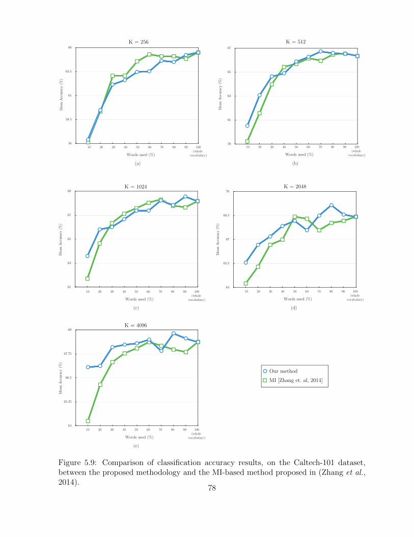
Mea
n A
ccura
cy (
%)
Mea
n A
ccura
cy (
%)
Mea
n A
ccura
cy (
%)
M
ean A
ccura
cy (
%)
Mea
n A
ccura
cy (
%)
K = 256 K = 512
K = 1024
K = 4096
K = 2048
(a) (b)
10 20 30 40 50 60 70 80 90 100(whole
vocabulary)Words used (%)
10 20 30 40 50 60 70 80 90 100(whole
vocabulary)Words used (%)
(c) (d)
10 20 30 40 50 60 70 80 90 100(whole
vocabulary)Words used (%)
(e)
10 20 30 40 50 60 70 80 90 100(whole
vocabulary)Words used (%)
10 20 30 40 50 60 70 80 90 100(whole
vocabulary)Words used (%)
Our method
MI [Zhang et. al, 2014]
56
58.5
61
63.5
66
59
61
63
65
67
61
63
65
67
69
64
65.5
67
68.5
70
64
65.25
66.5
67.75
69
Figure 5.9: Comparison of classification accuracy results, on the Caltech-101 dataset,between the proposed methodology and the MI-based method proposed in (Zhang et al.,2014).
78

As it can be seen in Figure 5.9, for each value of K used in the experiment, our proposal
obtains the best classification accuracy results for the highest compression rates. Besides,
for the other filtering sizes our proposal and the MI-based method attains comparable
results.
5.2.3 Computation Time of the Visual Vocabulary Ranking
The computation time of the visual vocabulary ranking methodology has also been eval-
uated. Table 5.3 shows the time in seconds taken for the ranking method in different size
vocabularies, for the Caltech-101 and the Pascal VOC 2006 dataset. In Table 5.3, the
ranking time is compared with the time needed to build the visual vocabulary.
As can be seen in Table 5.3, the proposed methodology can be used to improve visual
vocabularies without requiring much extra computation time.
5.3 Summary
In this chapter we devised a methodology for reducing the size of visual vocabularies
that allows to obtain more discriminative and representative visual vocabularies for BoW
image representation. The vocabulary reduction is based on three properties and their
corresponding quantitative measures that express the inter-class representativeness, the
intra-class representativeness and inter-class distinctiveness of visual words. The exper-
imental results presented in this chapter showed that, in average, with only 25% of the
ranked vocabulary, statistically superior classification results can be obtained, compared
to the classical BoW representation using the entire vocabularies. Therefore, the proposed
method, in addition to providing accuracy improvements, provides a substantial efficiency
improvement. Also, compared with a mutual information based method our proposal ob-
tained superior results for the highest compression rates and comparable results for the
other filtering sizes. The method proposed in this Chapter provides a discriminative,
representative and compact appearance representation of the object hypotheses formed
by the OCTAR method, presented in Chapter 4.
79

Chapter 6
Conclusions
6.1 Summary and Conclusions
Shape information has shown to be useful in the representation of category-level objects,
even in the presence of partial occlusion, changes in rotation, translation and scale, and
noise in the contour.
As a result of this work, a method for shape feature extraction, description and match-
ing of binary images, invariant to rotation, translation and scale, has been developed. The
proposed method allowed to overcome the intrinsic disadvantages of only using local or
global features by capturing the local structure of shape and later using it holistically for
matching. In the conducted experiments, our method showed larger robustness to partial
occlusion than other methods in the state of the art. Also, the proposal of a massively
parallel implementation in CUDA of the two most time-consuming stages of LISF showed
that significant speed-ups could be achieved, improving the efficiency of the systems.
In order to deal with the intrinsic problems derived from using edges extracted from
real images, it was necessary to propose a shape descriptor that was particularly suitable
for partial shape matching of both open and closed contours extracted from edgemap im-
ages. Furthermore, to propose a partial shape matching method robust to partial occlu-
sion, noise, rotation and translation in the contour was needed. The use of a self-containing
shape descriptor has shown to be essential for obtaining partial matches efficiently. The
contour fragments configuration descriptor had a key role in forming object hypotheses
80

coherently with the model, allowing to analyze the spatial relations and structure between
edge fragments that could be joined to form an object hypothesis.
Appearance information has shown to provide important cues for object recognition.
By combining shape and appearance through the evaluation of the appearance of the
shape-based object detection hypotheses, allowed us to better discriminate object hy-
potheses, particularly in those classes with distinctive texture. Under the BoW approach,
the results presented in this thesis, showed that not every visual word has the same rele-
vance for the object representation. Using information about the class and object labels
of the features in the visual vocabulary allowed us to obtain a more compact, discrimi-
native and representative visual vocabulary, with considerable improvements in accuracy
and efficiency.
6.2 Main Contributions
The main contributions of this thesis are:
a) A shape-based object recognition method, named LISF, that is invariant to rotation,
translation and scale, and present certain robustness to partial occlusion. LISF,
for highly occluded images largely outperformed other popular shape description
methods and retain comparable results for not occluded images.
b) A massively parallel implementation in CUDA of the two most time-consuming
stages of LISF, i.e., the feature extraction and feature matching steps, which
achieves speed-ups of up to 32x and 34x, respectively.
c) A shape-based object recognition method, named OCTAR, able to deal with the
intrinsic problems derived from using edges extracted from real images, i.e., bro-
ken and missing edge fragments that represent the target object, edge fragment
wrongly connected to another object or background edges, and background clutter-
ing. OCTAR, for highly occluded images largely outperformed other popular shape
81

description methods and retained comparable results for not occluded images. Also,
outperformed other methods in the state of the art in object detection in real images.
d) Three properties and their corresponding quantitative evaluation measures to as-
sess the ability of a visual word to represent and discriminate an object class, in
the context of the BoW approach. Also, based on these properties, we proposed
a methodology for reducing the size of the visual vocabulary, retaining those vi-
sual words that best describe an object class. Using our reduced vocabularies the
classification performance is improved with a significant reduction of the image rep-
resentation size.
The combination of these contributions is a step forward on the development of the
field of object recognition, an important and still open problem in Computer Vision.
6.3 Future Work
The results obtained in this thesis did not conclude the studies on shape and appearance-
based category-level object recognition. Based on the obtained results, we propose as
future work:
a) The OCTAR descriptor also provides information of the concavity/convexity of the
contour. This information could be used to generate a binary OCTAR descriptor,
based on its sign (concavity/convexity). The binary OCTAR descriptor could be
used for shape indexing or for discarding not relevant object hypotheses with a
smaller computational cost.
b) To propose a massively parallel implementation in GPU of the OCTAR method,
specifically for the matching and hypotheses building stages.
c) The properties of visual words and their corresponding quantitative measures pro-
posed in Chapter 5 could be further explored in order to propose a weighting schema
82

to improve image representation, to propose a classifier that makes use of such infor-
mation about the attributes and to define a measure that help us to automatically
choose the more adequate filter size.
6.4 Publications
The following publications were generated as result of this doctoral research:
1. Leonardo Chang, Airel Perez-Suarez, Miguel Arias-Estrada, Jose Hernandez-
Palancar, and L. Enrique Sucar. Improving visual vocabularies: a more discrimina-
tive, representative and compact bag of visual words. Submitted to Machine Vision
and Applications journal. May 2014.
2. Leonardo Chang, Miriam M. Duarte, L. Enrique Sucar, and Eduardo F. Morales. A
Bayesian approach for object classification based on clusters of SIFT local features.
Expert Systems with Applications. 39, 2 (February 2012), 1679-1686, 2012.
3. Leonardo Chang, Miguel Arias-Estrada, L. Enrique Sucar, and Jose Hernandez
Palancar. LISF: An invariant local shape features descriptor robust to occlusion.
In ICPRAM 2014 - Proceedings of the 3rd International Conference on Pattern
Recognition Applications and Methods, ESEO, Angers, Loire Valley, France, 6-8
March, 2014, pages 429437, 2014.
4. Leonardo Chang, Miguel Arias-Estrada, Jose Hernandez-Palancar, and L. Enrique
Sucar. Partial shape matching and retrieval under occlusion and noise. In Progress
in Pattern Recognition, Image Analysis, Computer Vision, and Applications - 19th
Iberoamerican Congress, CIARP 2014, Puerto Vallarta, Mexico, November 2-5,
2014. Proceedings, pages 151158, 2014.
5. Leonardo Chang, Miguel Arias-Estrada, Jose Hernandez-Palancar, and L. Enrique
Sucar. An Efficient Shape Feature Extraction, Description and Matching Method
using GPU. In Maria De Marsico, Antoine Tabbone and Ana Fred editors, ICPRAM
2014 - Best Papers, Lecture Notes in Computer Science. Springer. 2014.
83

6. Leonardo Chang, Miguel Arias-Estrada, L. Enrique Sucar, and Jose Hernandez
Palancar. Efficient Extraction and Matching of LISF Features in GPU. Poster
Session of GTC 2014: GPU Technology Conference 2014, San Jose California, USA,
2014.
7. Leonardo Chang, Miguel Arias-Estrada, L. Enrique Sucar, and Jose Hernandez
Palancar. Efficient Local Shape Features Matching using CUDA. Poster Session of
GTC 2013: GPU Technology Conference 2013, San Jose California, USA, 2013.
8. Leonardo Chang, Airel Perez-Suarez, Maximo Rodrıguez-Collada, Jose Hernandez-
Palancar, Miguel Arias-Estrada and L. Enrique Sucar. Assessing the Distinctiveness
and Representativeness of Visual Vocabularies. Submitted to CIARP 2015.
9. Leonardo Chang, Miguel Arias-Estrada, Jose Hernandez-Palancar, and L. Enrique
Sucar. Object Detection through Partial Contour Fragments Matching. Submitted
to CIARP 2015.
84

Bibliography
(2013) Concepts and applications of inferential statistics. URL
http://vassarstats.net/textbook/. URL http://vassarstats.net/textbook/
Adamek T, O’Connor NE (2004) A multiscale representation method for nonrigid shapes
with a single closed contour. IEEE Trans Circuits Syst Video Techn 14(5):742–753,
URL http://dblp.uni-trier.de/db/journals/tcsv/tcsv14.html#AdamekO04
Agarwal S, Awan A, Roth D (2004) Learning to detect objects in images via a sparse, part-
based representation. IEEE Transactions on Pattern Analysis and Machine Intelligence
26(11):1475–1490, URL http://www.ncbi.nlm.nih.gov/pubmed/15521495
Agin GJ, Binford TO (1976) Computer Description of Curved Objects. IEEE Trans-
actions on Computers C-25(4):439–449, DOI 10.1109/TC.1976.1674626, URL http:
//ieeexplore.ieee.org/lpdocs/epic03/wrapper.htm?arnumber=1674626
Alajlan N, Rube IE, Kamel MS, Freeman G (2007) Shape retrieval using triangle-area rep-
resentation and dynamic space warping. Pattern Recognition 40(7):1911 – 1920, DOI
http://dx.doi.org/10.1016/j.patcog.2006.12.005, URL http://www.sciencedirect.
com/science/article/pii/S0031320306005188
Asada H, Brady M (1986) The curvature primal sketch. IEEE Transactions on Pat-
tern Analysis and Machine Intelligence 8(1):2–14, URL http://ieeexplore.ieee.
org/lpdocs/epic03/wrapper.htm?arnumber=4767747
Bai X, Yang X, Latecki LJ, Liu W, Tu Z (2010) Learning context-sensitive shape similarity
by graph transduction. IEEE Trans Pattern Anal Mach Intell 32(5):861–874
85
Bay H, Ess A, Tuytelaars T, Van Gool L (2008) Speeded-Up Robust Features (SURF).
Comput Vis Image Underst 110(3):346–359, DOI http://dx.doi.org/10.1016/j.cviu.
2007.09.014
Belongie S, Malik J, Puzicha J (2001) Matching shapes. In: Proceedings Eighth IEEE
International Conference on Computer Vision ICCV 2001, IEEE, IEEE Comput. Soc,
vol 1, pp 454–461, DOI 10.1109/ICCV.2001.937552, URL http://ieeexplore.ieee.
org/lpdocs/epic03/wrapper.htm?arnumber=937552
Belongie S, Malik J, Puzicha J (2002) Shape matching and object recognition using shape
contexts. IEEE Transactions on Pattern Analysis and Machine Intelligence 24(4):509–
522, DOI 10.1109/34.993558, URL http://ieeexplore.ieee.org/lpdocs/epic03/
wrapper.htm?arnumber=993558
Besl PJ, McKay ND (1992) A method for registration of 3-d shapes. IEEE Trans Pattern
Anal Mach Intell 14(2):239–256, DOI 10.1109/34.121791, URL http://dx.doi.org/
10.1109/34.121791
Biederman I (1985) Human image understanding: Recent research and a the-
ory. Computer Vision Graphics and Image Processing 32(1):29–73, DOI 10.1016/
0734-189x(85)90002-7, URL http://www.sciencedirect.com/science/article/
pii/0734189X85900027
Biederman I, Ju G (1988) Surface versus edge-based determinants of visual recognition.
Cognitive Psychology 20(1):38–64, URL http://www.ncbi.nlm.nih.gov/pubmed/
3338267
Binford TO (1971) Visual Perception by Computer. In: Grasselli A (ed) IEEE Conference
on Systems and Control, IEEE, pp 277–284
Blum H (1967) A transformation for extracting new descriptors of shape. Models for the
perception of speech and visual form 19(5):362–380, URL http://pageperso.lif.
univ-mrs.fr/~edouard.thiel/rech/1967-blum.pdf
86

Bosch A, Zisserman A, Munoz X (2007) Image classification using random forests and
ferns. IEEE 11th International Conference on Computer Vision (2007) 23(1):1–8, URL
http://eprints.pascal-network.org/archive/00003046/
Bouchard G, Triggs W (2005) Hierarchical part-based visual object categorization.
2005 IEEE Computer Society Conference on Computer Vision and Pattern Recog-
nition CVPR05 1:710–715, URL http://eprints.pascal-network.org/archive/
00000801/
Brooks RA (1983) Model-Based 3-D Interpretation of 2-D Images. IEEE Transactions on
Pattern Recognition and Machine Intelligence PAMI-5(2):140–150
Carneiro G, Lowe D (2006) Sparse Flexible Models of Local Features. 9th European
Conference on Computer Vision ECCV 2006 3953:29–43, DOI 10.1007/11744078, URL
http://www.springerlink.com/content/u7l072qn26147501
Chandra S, Kumar S, Jawahar CV (2012) Learning hierarchical bag of words using naive
bayes clustering. In: Asian Conference on Computer Vision, pp 382–395
Chang L, Duarte M, Sucar L, Morales E (2010) Object Class Recognition Using SIFT
and Bayesian Networks. Advances In Soft Computing pp 56—-66, URL http://www.
springerlink.com/index/454413323066V860.pdf
Chang L, Duarte MM, Sucar LE, Morales EF (2012) A bayesian approach for object
classification based on clusters of sift local features. Expert Systems with Applica-
tions 39:1679–1686, DOI http://dx.doi.org/10.1016/j.eswa.2011.06.059, URL http:
//dx.doi.org/10.1016/j.eswa.2011.06.059
Chang L, Arias-Estrada M, Palancar JH, Sucar LE (2014a) Partial shape matching and
retrieval under occlusion and noise. In: Progress in Pattern Recognition, Image Anal-
ysis, Computer Vision, and Applications - 19th Iberoamerican Congress, CIARP 2014,
Puerto Vallarta, Mexico, November 2-5, 2014. Proceedings, pp 151–158, DOI 10.1007/
978-3-319-12568-8 19, URL http://dx.doi.org/10.1007/978-3-319-12568-8_19
87
Chang L, Arias-Estrada MO, Sucar LE, Palancar JH (2014b) Lisf: An invariant local
shape features descriptor robust to occlusion. In: Marsico MD, Tabbone A, Fred ALN
(eds) ICPRAM 2014 - Proceedings of the 3rd International Conference on Pattern
Recognition Applications and Methods, ESEO, Angers, Loire Valley, France, 6-8 March,
2014, SciTePress, pp 429–437, DOI http://dx.doi.org/10.5220/0004825504290437
Chen Y, Medioni G (1992) Object modelling by registration of multiple range images.
Image Vision Comput 10(3):145–155, DOI 10.1016/0262-8856(92)90066-C, URL http:
//dx.doi.org/10.1016/0262-8856(92)90066-C
Chetverikov D (2003) A Simple and Efficient Algorithm for Detection of High Curvature
Points in Planar Curves. Proceedings of the 23rd Workshop of the Austrian Pattern
Recognition Group pp 746–753, DOI 10.1007/978-3-540-45179-2\ 91, URL http://
www.springerlink.com/index/VN2RGLUK251H3XCC.pdf
Chong CW, Raveendran P, Mukundan R (2004) Translation and scale invariants of leg-
endre moments. Pattern Recognition 37(1):119–129
Csurka G, Dance CR, Fan L, Willamowski J, Bray C (2004) Visual categorization with
bags of keypoints. In: Workshop on Statistical Learning in Computer Vision, ECCV,
pp 1–22
De Winter J, Wagemans J (2004) Contour-based object identification and segmentation:
stimuli, norms and data, and software tools. Behavior research methods instruments
computers A journal of the Psychonomic Society Inc 36(4):604–624, URL http://www.
ncbi.nlm.nih.gov/pubmed/15641406
Dickinson SJ (2009) Object Categorization. Computer and Human Vision Perspectives,
Cambridge Books, chap The Evolution of Object Categorization and the Challenge of
Image Abstraction, pp 1–37
Direkoglu C, Nixon M (2011) Shape classification via image-based multiscale description.
Pattern Recognition 44(9):2134–2146, URL http://eprints.soton.ac.uk/272192/
88

Dork G, Schmid C (2005) Object class recognition using discriminative local features.
Tech. rep., IEEE Transactions on Pattern Analysis and Machine Intelligence
Elkan C (2003) Using the triangle inequality to accelerate k-means. In: Fawcett T, Mishra
N (eds) ICML, AAAI Press, pp 147–153
Emerson P (2013) The original borda count and partial voting. Social Choice and Welfare
40(2):353–358
Everingham M, Zisserman A, Williams CKI, Van Gool L (2006) The PASCAL
Visual Object Classes Challenge 2006 (VOC2006) Results. http://www.pascal-
network.org/challenges/VOC/voc2006/results.pdf
Everingham M, Van Gool L, Williams CKI, Winn J, Zisserman A (2011) The PAS-
CAL Visual Object Classes Challenge 2011 (VOC2011) Results. http://www.pascal-
network.org/challenges/VOC/voc2011/workshop/index.html
Fei-fei L, Fergus R, Perona P (2003) A Bayesian approach to unsupervised one-shot
learning of object categories. Proceedings Ninth IEEE International Conference on
Computer Vision 2(Iccv):1134–1141 vol.2, DOI 10.1109/ICCV.2003.1238476, URL
http://ieeexplore.ieee.org/lpdocs/epic03/wrapper.htm?arnumber=1238476
Fei-Fei L, Fergus R, Perona P (2007) Learning generative visual models from few training
examples: An incremental bayesian approach tested on 101 object categories. Comput
Vis Image Underst 106(1):59–70
Felzenszwalb PF, Huttenlocher DP (2005) Pictorial Structures for Object Recogni-
tion. International Journal of Computer Vision 61(1):55–79, DOI 10.1023/B:VISI.
0000042934.15159.49, URL http://www.springerlink.com/openurl.asp?id=doi:
10.1023/B:VISI.0000042934.15159.49
Felzenszwalb PF, McAllester DA, Ramanan D (2008) A discriminatively trained, mul-
tiscale, deformable part model. In: CVPR, IEEE Computer Society, URL http:
//dblp.uni-trier.de/db/conf/cvpr/cvpr2008.html#FelzenszwalbMR08
89

Fergus R, Perona P, Zisserman A (2003) Object class recognition by unsupervised scale-
invariant learning. In: Proceedings of the IEEE Conference on Computer Vision and
Pattern Recognition, Madison, Wisconsin, vol 2, pp 264–271
Fernando B, Fromont , Muselet D, Sebban M (2012) Supervised learning of gaussian
mixture models for visual vocabulary generation. Pattern Recognition 45(2):897–907
Ferrari V, Tuytelaars T, Gool LJV (2006) Object detection by contour segment networks.
In: Leonardis A, Bischof H, Pinz A (eds) ECCV (3), Springer, Lecture Notes in Com-
puter Science, vol 3953, pp 14–28, URL http://dblp.uni-trier.de/db/conf/eccv/
eccv2006-3.html#FerrariTG06
Ferrari V, Jurie F, Schmid C (2010) From images to shape models for object detection. In-
ternational Journal of Computer Vision 87(3):284–303, URL http://dblp.uni-trier.
de/db/journals/ijcv/ijcv87.html#FerrariJS10
Ferrie FP, Lagarde J, Whaite P (1993) Darboux Frames, Snakes, and Super-Quadrics:
Geometry from the Bottom Up. IEEE Transactions on Pattern Analysis and Machine
Intelligence 15(8):771–784, DOI 10.1109/34.236252
Gehler PV, Nowozin S (2009) On feature combination for multiclass object classification.
In: ICCV, IEEE, pp 221–228
Gong Y, Kumar S, Rowley HA, Lazebnik S (2013) Learning binary codes for high-
dimensional data using bilinear projections. In: CVPR 2013
Gonzalez-Aguirre DI, Hoch J, Rhl S, Asfour T, Bayro-Corrochano E, Dillmann R (2011)
Towards shape-based visual object categorization for humanoid robots. In: ICRA,
IEEE, pp 5226–5232, URL http://dblp.uni-trier.de/db/conf/icra/icra2011.
html#Gonzalez-AguirreHRABD11
Grimson WEL, Lozano-Perez T (1984) Model-Based Recognition and Localization from
Sparse Range or Tactile Data. The International Journal of Robotics Research 3(3):3–
90

35, DOI 10.1177/027836498400300301, URL http://ijr.sagepub.com/cgi/doi/10.
1177/027836498400300301
Hartigan JA, Wong MA (1979) A k-means clustering algorithm. JSTOR: Applied Statis-
tics 28(1):100–108
Hu MK (1962) Visual pattern recognition by moment invariants. IRE Transactions
on Information Theory 8(2):179–187, DOI 10.1109/TIT.1962.1057692, URL http:
//ieeexplore.ieee.org/xpls/abs_all.jsp?arnumber=1057692
Huttenlocher DP, Ullman S (1990) Recognizing solid objects by alignment with an im-
age. International Journal of Computer Vision 5(2):195–212, DOI 10.1007/BF00054921,
URL http://www.springerlink.com/index/10.1007/BF00054921
Jegou H, Douze M, Schmid C (2011) Product quantization for nearest neighbor search.
IEEE Pattern Analysis and Machine Intellingence 33(1):117–128
Jiu M, Wolf C, Garcia C, Baskurt A (2012) Supervised learning and codebook optimiza-
tion for bag of words models. Cognitive Computation 4:409–419
Kesorn K, Poslad S (2012) An enhanced bag-of-visual word vector space model to repre-
sent visual content in athletics images. IEEE Transactions on Multimedia 14(1):211–222
Khotanzad A, Hong YH (1988) Rotation invariant pattern recognition using zernike mo-
ments. Pattern Recognition, 1988, 9th International Conference on pp 326–328 vol.1,
DOI 10.1109/ICPR.1988.28233
Kim WY, Kim YS (2000) A region-based shape descriptor using Zernike mo-
ments. Signal Processing Image Communication 16(1-2):95–102, DOI 10.1016/
S0923-5965(00)00019-9, URL http://linkinghub.elsevier.com/retrieve/pii/
S0923596500000199
Kimia BB (2009) Shapes and Shock Graphs: From Segmented Shapes to Shapes Embed-
ded in Images, Cambridge University Press, p 430–450
91
Kirby M, Sirovich L (1990) Application of the Karhunen-Loeve procedure for the char-
acterization of human faces. IEEE Transactions on Pattern Analysis and Machine In-
telligence 12(1):103–108, DOI 10.1109/34.41390, URL http://ieeexplore.ieee.org/
lpdocs/epic03/wrapper.htm?arnumber=41390
Kliot M, Rivlin E (1998) Invariant-Based Shape Retrieval in Pictorial Databases. Com-
puter Vision and Image Understanding 71(2):182–197, DOI 10.1006/cviu.1998.0709,
URL http://linkinghub.elsevier.com/retrieve/pii/S1077314298907093
Latecki LJ, Lakmper R, Eckhardt U (2000) Shape descriptors for non-rigid shapes with a
single closed contour. In: CVPR, IEEE Computer Society, pp 1424–1429, URL http:
//dblp.uni-trier.de/db/conf/cvpr/cvpr2000.html#LateckiLE00
Lazebnik S, Schmid C, Ponce J (2006) Beyond Bags of Features: Spatial Pyramid Match-
ing for Recognizing Natural Scene Categories. 2006 IEEE Computer Society Conference
on Computer Vision and Pattern Recognition Volume 2 CVPR06 2(2169-2178):2169–
2178, URL http://eprints.pascal-network.org/archive/00002929/
Leibe B, Leonardis A, Schiele B (2004) Combined Object Categorization and
Segmentation with an Implicit Shape Model. Work 1(May):1–16, DOI 10.1.1.
5.6272, URL http://citeseerx.ist.psu.edu/viewdoc/download?doi=10.1.1.5.
6272&rep=rep1&type=pdf
Leibe B, Leonardis A, Schiele B (2007) Robust Object Detection with Interleaved Cat-
egorization and Segmentation. International Journal of Computer Vision 77(1-3):259–
289, DOI 10.1007/s11263-007-0095-3, URL http://www.springerlink.com/index/
10.1007/s11263-007-0095-3
Li T, Ye M, Ding J (2014) Discriminative hough context model for object detection.
The Visual Computer 30(1):59–69, URL http://dblp.uni-trier.de/db/journals/
vc/vc30.html#LiYD14
92

Ling H, Jacobs DW (2007) Shape classification using the inner-distance. IEEE TPAMI
29(2):286–299, URL http://dblp.uni-trier.de/db/journals/pami/pami29.html#
LingJ07
Liu G (2010) Improved bags-of-words algorithm for scene recognition. Journal of Compu-
tational Information Systems 6(14):4933 – 4940
Liu J, Shah M (2008) Learning human actions via information maximization. 2013 IEEE
Conference on Computer Vision and Pattern Recognition 0:1–8
Lopez-Sastre R, Tuytelaars T, Acevedo-Rodriguez F, Maldonado-Bascon S (2011) To-
wards a more discriminative and semantic visual vocabulary. Computer Vision and
Image Understanding 115(3):415 – 425, special issue on Feature-Oriented Image and
Video Computing for Extracting Contexts and Semantics
Lowe DG (1999) Object recognition from local scale-invariant features. Proceedings
of the Seventh IEEE International Conference on Computer Vision 2([8):1150–1157
vol.2, DOI 10.1109/ICCV.1999.790410, URL http://ieeexplore.ieee.org/lpdocs/
epic03/wrapper.htm?arnumber=790410
Lowe DG (2004) Distinctive image features from scale-invariant keypoints. Interna-
tional Journal of Computer Vision 60(2):91–110, DOI http://dx.doi.org/10.1023/B:
VISI.0000029664.99615.94
Lu Z, Ip HHS (2009) Image categorization with spatial mismatch kernels. In: CVPR,
IEEE, pp 397–404
Ma T, Latecki LJ (2011) From partial shape matching through local deformation to
robust global shape similarity for object detection. In: CVPR, IEEE, pp 1441–1448,
URL http://dblp.uni-trier.de/db/conf/cvpr/cvpr2011.html#MaL11
Maji S, Malik J (2009) Object detection using a max-margin hough transform. In: CVPR,
IEEE, pp 1038–1045, URL http://dblp.uni-trier.de/db/conf/cvpr/cvpr2009.
html#MajiM09
93

Mann HB, Whitney DR (1947) On a test of whether one of two random variables is
stochastically larger than the other. Annals of Mathematical Statistics 18(1):50–60
Martin DR, Fowlkes CC, Malik J (2004) Learning to detect natural image bound-
aries using local brightness, color, and texture cues. IEEE TPAMI 26(5):530–
49, DOI 10.1109/TPAMI.2004.1273918, URL http://ieeexplore.ieee.org/xpl/
articleDetails.jsp?arnumber=1273918
Martınez JM (2004) MPEG-7 Overview. URL http://www.chiariglione.org/mpeg/standards/mpeg-
7/mpeg-7.htm. URL http://www.chiariglione.org/mpeg/standards/mpeg-7/
mpeg-7.htm
Matas J (2004) Robust wide-baseline stereo from maximally stable extremal regions.
Image and Vision Computing 22(10):761–767, DOI 10.1016/j.imavis.2004.02.006, URL
http://linkinghub.elsevier.com/retrieve/pii/S0262885604000435
McNeill G, Vijayakumar S (2006) Hierarchical procrustes matching for shape retrieval.
In: CVPR (1), IEEE Computer Society, pp 885–894, URL http://dblp.uni-trier.
de/db/conf/cvpr/cvpr2006-1.html#McNeillV06
Mikolajczyk K (2004) Scale & Affine Invariant Interest Point Detectors. Interna-
tional Journal of Computer Vision 60(1):63–86, DOI 10.1023/B:VISI.0000027790.
02288.f2, URL http://www.springerlink.com/openurl.asp?id=doi:10.1023/B:
VISI.0000027790.02288.f2
Mikolajczyk K, Schmid C (2002) An affine invariant interest point detector. Im-
age Rochester NY 1(1):128–142, DOI 10.1007/3-540-47969-4, URL http://www.
springerlink.com/openurl.asp?id=doi:10.1023/B:VISI.0000027790.02288.f2
Mikolajczyk K, Leibe B, Schiele B (2005) Local features for object class recognition.
In: ICCV ’05: Proceedings of the Tenth IEEE International Conference on Computer
Vision, IEEE Computer Society, Washington, DC, USA, pp 1792–1799, DOI http:
//dx.doi.org/10.1109/ICCV.2005.146
94
Mokhtarian F, Bober M (2003) Curvature Scale Space Representation: Theory, Applica-
tions, and MPEG-7 Standardization. Kluwer
Murase H, Nayar SK (1995) Visual learning and recognition of 3-d objects from appear-
ance. International Journal of Computer Vision 14(1):5–24, DOI 10.1007/BF01421486,
URL http://www.springerlink.com/index/10.1007/BF01421486
Pentland AP (1986) Perceptual organization and the representation of natural form.
Artificial Intelligence 28(3):293–331, DOI 10.1016/0004-3702(86)90052-4, URL http:
//linkinghub.elsevier.com/retrieve/pii/0004370286900524
Qin J, Yung NHC (2012) Feature fusion within local region using localized maximum-
margin learning for scene categorization. Pattern Recognition 45(4):1671–1683
Riemenschneider H, Donoser M, Bischof H (2010) Using partial edge contour matches for
efficient object category localization. In: ECCV’10, Springer-Verlag, Berlin, Heidelberg,
pp 29–42, URL http://dl.acm.org/citation.cfm?id=1888150.1888154
Roh KS, Kweon IS (1998) 2-d object recognition using invariant contour descriptor
and projective refinement. Pattern Recognition 31(4):441–455, URL http://dblp.
uni-trier.de/db/journals/pr/pr31.html#RohK98
Rube IE, Alajlan N, Kamel M, Ahmed M, Freeman GH (2005) Robust multiscale triangle-
area representation for 2d shapes. In: ICIP (1), IEEE, pp 545–548, URL http://dblp.
uni-trier.de/db/conf/icip/icip2005-1.html#RubeAKAF05
Rublee E, Rabaud V, Konolige K, Bradski G (2011) ORB: An efficient alternative to
SIFT or SURF. In: International Conference on Computer Vision, Barcelona
Sebastian TB, Klein PN, Kimia BB (2004) Recognition of shapes by editing their shock
graphs. IEEE Transactions on Pattern Analysis and Machine Intelligence 26(5):550–
571, DOI 10.1109/TPAMI.2004.1273924, URL http://dx.doi.org/10.1109/TPAMI.
2004.1273924
95
Shu X, Wu XJ (2011) A novel contour descriptor for 2D shape matching and its ap-
plication to image retrieval. Image and Vision Computing 29(4):286–294, DOI 10.
1016/j.imavis.2010.11.001, URL http://linkinghub.elsevier.com/retrieve/pii/
S0262885610001526
Silberberg TM, Harwood DA, Davis LS (1986) Object recognition using oriented model
points. Comput Vision Graph Image Process 35:47–71, DOI 10.1016/0734-189X(86)
90125-8, URL http://dl.acm.org/citation.cfm?id=16504.16507
Solina F, Bajcsy R (1990) Recovery of Parametric Models from Range Images: The
Case for Superquadrics with Global Deformations. IEEE Transactions on Pattern
Analysis and Machine Intelligence 12(2):131–147, DOI 10.1109/34.44401, URL http:
//ieeexplore.ieee.org/lpdocs/epic03/wrapper.htm?arnumber=44401
Srinivasan P, Zhu Q, Shi J (2010) Many-to-one contour matching for describing and
discriminating object shape. In: The Twenty-Third IEEE Conference on Computer
Vision and Pattern Recognition, CVPR 2010, San Francisco, CA, USA, 13-18 June
2010, pp 1673–1680, DOI 10.1109/CVPR.2010.5539834, URL http://dx.doi.org/
10.1109/CVPR.2010.5539834
Stark M, Schiele B (2007) How Good are Local Features for Classes of Geometric Objects.
IEEE 11th International Conference on Computer Vision (2007) pp 1–8, DOI 10.1109/
ICCV.2007.4408878, URL http://ieeexplore.ieee.org/lpdocs/epic03/wrapper.
htm?arnumber=4408878
Terzopoulos D, Metaxas D (1991) Dynamic 3D Models with Local and Global Deforma-
tions. IEEE Trans Pattern Anal Machine Intell 13(7):703–714
Toshev A, Taskar B, Daniilidis K (2011) Shape-based Object Detection via Bound-
ary Structure Segmentation. International Journal of Computer Vision 99(2):123–
146, DOI 10.1007/s11263-012-0521-z, URL http://www.springerlink.com/content/
u7170160440l086x/
96

Trinh NH, Kimia BB (2011) Skeleton Search: Category-Specific Object Recognition and-
Segmentation Using a Skeletal Shape Model. International Journal of Computer Vision
94(2):215–240, DOI 10.1007/s11263-010-0412-0, URL http://www.springerlink.
com/index/10.1007/s11263-010-0412-0
Tsai CF (2012) Bag-of-words representation in image annotation: A review. ISRN Arti-
ficial Intelligence 2012
Turk M, Pentland A (1991) Eigenfaces for recognition. DOI 10.1162/jocn.1991.3.1.71,
URL http://www.mitpressjournals.org/doi/abs/10.1162/jocn.1991.3.1.71
Tuytelaars T, Mikolajczyk K (2007) Local invariant feature detectors: A survey. Foun-
dations and Trends in Computer Graphics and Vision 3(3):177–280, URL http:
//dblp.uni-trier.de/db/journals/ftcgv/ftcgv3.html
Van Otterloo PJ (1991) A contour-oriented approach to shape analysis. Prentice Hall
International (UK) Ltd., Hertfordshire, UK, UK
Vedaldi A, Fulkerson B (2008) VLFeat: An open and portable library of computer vision
algorithms
Vedaldi A, Zisserman A (2011) Efficient additive kernels via explicit feature maps. Pattern
Analysis and Machine Intellingence 34(3)
Wang X, Bai X, Ma T, Liu W, Latecki LJ (2012) Fan shape model for object de-
tection. In: CVPR, IEEE, pp 151–158, URL http://dblp.uni-trier.de/db/conf/
cvpr/cvpr2012.html#WangBMLL12
Weber M, Welling M, Perona P (2000) Towards Automatic Discovery of Object Cate-
gories. Electrical Engineering 2(1063):101–108, DOI 10.1109/CVPR.2000.854754, URL
http://ieeexplore.ieee.org/xpls/abs_all.jsp?arnumber=854754
Wu J, Tan WC, Rehg JM (2011) Efficient and effective visual codebook generation using
additive kernels. Journal of Machine Learning Research 12:3097–3118
97

Yang X, Kknar-tezel S, Latecki LJ (2009) Locally constrained diffusion process on locally
densified distance spaces with applications to shape retrieval. In: In: Proc. IEEE Conf.
on Computer Vision and Pattern Recognition (CVPR
Yang X, Bai X, Kknar-Tezel S, Latecki L (2013) Densifying distance spaces for shape
and image retrieval. Journal of Mathematical Imaging and Vision 46(1):12–28, DOI
10.1007/s10851-012-0363-x, URL http://dx.doi.org/10.1007/s10851-012-0363-x
Zhang D (2004) Review of shape representation and description techniques. Pattern
Recognition 37(1):1–19, DOI 10.1016/j.patcog.2003.07.008, URL http://linkinghub.
elsevier.com/retrieve/pii/S0031320303002759
Zhang D, Lu G (2002a) Generic Fourier descriptor for shape-based image retrieval. Pro-
ceedings IEEE International Conference on Multimedia and Expo 1(1):425–428, DOI
10.1109/ICME.2002.1035809, URL http://ieeexplore.ieee.org/lpdocs/epic03/
wrapper.htm?arnumber=1035809
Zhang D, Lu G (2002b) Shape based image retrieval using generic fourier descriptors. In:
Signal Processing: Image Communication 17, pp 825–848
Zhang J, Marszaek M, Lazebnik S, Schmid C (2007) Local Features and Kernels for
Classification of Texture and Object Categories: A Comprehensive Study. Interna-
tional Journal of Computer Vision 73(2):213–238, DOI 10.1007/s11263-006-9794-4,
URL http://www.springerlink.com/index/10.1007/s11263-006-9794-4
Zhang S, Tian Q, Hua G, Huang Q, Gao W (2011a) Generating descriptive visual words
and visual phrases for large-scale image applications. IEEE Transactions on Image
Processing 20(9):2664–2677
Zhang S, Tian Q, Hua G, Zhou W, Huang Q, Li H, Gao W (2011b) Modeling spatial
and semantic cues for large-scale near-duplicated image retrieval. Computer Vision and
Image Understanding 115(3):403–414
98

Zhang Y, Wu J, Cai J (2014) Compact representation for image classification: To choose
or to compress? In: CVPR 2014
99

Appendix A
The Mann-Whitney Test
The Mann-Whitney U-test (Mann and Whitney, 1947) is used to test whether two in-
dependent samples of observations are drawn from the same or identical distributions.
Specifically, in Section 5.2.1, the Mann-Whitney test is used to verify that the results
obtained by the proposed method, are statistically superior to those obtained by the
baseline.
This test is based on the idea that the particular pattern exhibited when m number
of X random variables and n number of Y random variables are arranged together in
increasing order of magnitude provides information about the relationship between their
parent populations.
The Mann-Whitney test criterion is based on the magnitude of the Y ’s in relation to
the X’s, i.e., the position of Y ’s in the combined ordered sequence. A sample pattern of
arrangement where most of the Y ’s are greater than most of the X’s or vice versa would
be evidence against random mixing. This would tend to discredit the null hypothesis of
identical distribution.
The test has two important assumptions. First the two samples under consideration
are random, and are independent of each other, as are the observations within each sample.
Second the observations are numeric or ordinal (arranged in ranks). In our application
of the test, the two considered samples were the results of the baseline method, against
the best result obtained by our proposed method. A test for each dataset and each used
classifier was performed (see Tables 5.1 and 5.2).
100
In order to calculate the U statistics, the combined set of data is first arranged in
ascending order with tied scores receiving a rank equal to the average position of those
scores in the ordered sequence.
Let T denote the sum of ranks for the first sample. The Mann-Whitney test statistic
is then calculated using U = n1n2 + n1(n1 + 1)/2 − T , where n1 and n2 are the sizes of
the first and second samples respectively.
We next compare the value of calculated U with the value given in the Tables of
Critical Values for the Mann-Whitney U-test, where the critical values are provided for
given n1 and n2 , and accordingly accept or reject the null hypothesis. Even though the
distribution of U is known, the normal distribution provides a good approximation in case
of large samples.
In order to perform our tests, we used the Mann-Whitney Test implementation pro-
vided in the VassarStats website (vas, 2013).
101

102

Appendix B
Acronyms
SIFT Scale-Invariant Feature TransformSURF Speeded Up Robust FeaturesORB Oriented FAST and Rotated BRIEFMSER Maximally Stable Extremal RegionsGPU Graphics Processing Unit3D Three-dimensionalGPGPU General-Purpose Computing on Graphics Processing UnitsCAD Computer Aided DesignBoW Bag of WordsCSS Curvature Scale SpaceMCC Multi-scale Convexity ConcavitySC Shape ContextTAR Triangle-Area RepresentationMTAR Multi-scale Triangle-Area RepresentationGMM Gaussian Mixed ModelHIK Histogram Intersection KernelLISF Invariant Local Shape FeaturesCUDA Compute Unified Device ArchitectureRGB Red, Green and BlueOCTAR Open/Closed contours Triangle Area RepresentationICP Iterative Closest PointIDSC Inner Distance Shape ContextCPU Central Processing UnitGHz GigaHertzRAM Random-Access MemoryGB GigaBytePC Personal ComputerSVM Support Vector MachineKNN K-Nearest Neighbortf Term frecuencytf − idf Term frequency - inverse document frequencyfps Frames per second
103

Appendix C
Notations
dmin Lower scale limit for the LISF feature extraction methoddmax Upper scale limit for the LISF feature extraction methodαmin Lower sharpness limit for the LISF feature extraction methodαmax Upper sharpness limit for the LISF feature extraction methodHi LISF feature descriptorΩ Matching measure of LISF methodTAR(i, j, k) Signed area of the triangle formed by points i, j, kΘP(i, j) OCTAR descriptor value for points pair (i, j)Φ(P,Q) Similarity measure between two OCTAR descriptors ΘP and ΘQ
ΘP,R OCTAR spatial configuration descriptor of two contour fragments P and RECOV OCTAR covering criterionEZ OCTAR object hypothesis contour estimation criterionEZ∗ OCTAR fitted object hypothesis criterionEApp OCTAR appearance-based evaluation criterionM1(k, cj) Inter-class representativeness measure of class cj in visual word kM2(k, cj) Intra-class Representativeness Measure of class cj in visual word kM3(k,M) Distinctiveness measure of a given visual word k for a given measure M
104