an iterative algorithm for extending learners to a semi-supervised setting

An Iterative Algorithm for Extending Learners

to a Semi-supervised Setting

Mark Culp George Michailidis

October 17, 2007

Abstract

In this paper, we present an iterative self-training algorithm, whose objective is to extend learn-

ers from a supervised setting into a semi-supervised setting. The algorithm is based on using the

predicted values for observations where the response is missing (unlabeled data) and then incorpo-

rates the predictions appropriately at subsequent stages. Convergence properties of the algorithm

are investigated for particular learners, such as linear/logistic regression and linear smoothers with

particular emphasis on kernel smoothers. Further, implementation issues of the algorithm with other

learners such as generalized additive models, tree partitioning methods, partial least squares, etc. are

also addressed. The connection between the proposed algorithm and graph-based semi-supervised

learning methods is also discussed. The algorithm is illustrated on a number of real data sets using a

varying degree of labeled responses.

Keywords: Semi-supervised learning, linear smoothers, convergence, iterative algorithm

1 Introduction and Problem Formulation

In the supervised learning problem, the objective is to construct a rule (learner) based on training data

that would be capable of predicting accurately the response of future observations. Specifically, let

[Y |X] be a n × (p + 1) data matrix, with either a numerical or categorical response variable Y , and

p explanatory variables X . Over the years, several approaches have been proposed in the literature to

address the problem of constructing a learner φ(X, Y ) from the available training data for predicting the

response of any observation. Examples of such learners include various parametric and non-parametric

1

regression techniques for numerical responses and a number of classification algorithms for categorical

ones (see Ripley (1996), Duda et al. (2000), and Hastie et al. (2001)).

In many application areas, it is fairly simple and inexpensive to collect data on the p explanatory

variables. However, it is more challenging and expensive to observe the response Y for a large number

of observations. Such is the case with the pharmacology data set examined in Section 4. In such a setting,

data have been collected for p explanatory variables on n objects (cases), as before. But responses are

available only for a subset of size m of the objects; therefore, the data can be partitioned into two subsets:

the first set, of size m×(p+1) contains labeled data [YL|XL], while the second set of size (n−m)×(p+1)

contains unlabeled data [YU |XU ]. In particular, the response vector YU is missing. This gives rise to a

semi-supervised learning framework. The task at hand is to use the information available in the labeled

data, in conjunction with their relationship to unlabeled data, to better predict the information in XU

and potentially better predict any possible observation x. The problem of semi-supervised learning has

been studied from various perspectives, with emphasis on how the algorithm actually uses the unlabeled

information, and whether the proposed technique is transductive, that is, it can only complete the labeling

of the missing n−m responses, or inductive, in that it can predict the labels of any potential observation

(Krishnapuram et al., 2005). The survey by Zhu (2006) and the book by Chapelle et al. (2006b) provide a

nice overview of the field. Next, we provide a brief discussion highlighting some of the general problems

addressed in the area of semi-supervised learning.

One class of techniques is based on the following self-training idea. The most confident predictions

of unlabeled responses are successively added to the labeled set, and used in subsequent rounds for train-

ing the learner to predict less confident unlabeled observations. This approach tends to work best when

the number of unlabeled observations considered at each round is randomly selected, and the number

of observations added to the set is small relative to the size of the unlabeled data (Blum and Mitchell,

1998). Given the fact that in this context unlabeled (missing) response information is processed, most

such approaches are based on an EM algorithmic implementation, with fairly strong assumptions made

on the densities of the unlabeled data. These techniques have proved successful in a number of applica-

tion areas, including text classification and word sense disambiguation problems (Abney, 2004), image

processing (Baluja, 1999), and face recognition (Nigam et al., 2000). Another technique for extending

supervised borders into semi-supervised learning is the transductive support vector machine (TSVM)

(Vapnik, 1998). The main idea is to optimally push the border determined by a supervised margin-based

procedure away from highly dense regions of labeled and unlabeled data, which should minimize the

generalization error. The main challenge for this problem stems from the fact that the TSVM solution

is NP-hard. As a result, the implementation requires approximations to perform this task, which typi-

2

cally involve solving computationally intensive non-convex loss/penalty optimization problems (Vapnik,

1998; Chapelle et al., 2006a). The authors in Chapelle et al. (2006a) provide compelling quantitative

evidence that the global optimum of TSVM is quite accurate on small data sets.

Graph-based algorithms provide another class of semi-supervised procedures. The main idea is that

the data are represented by a graph, whose vertices are both labeled and unlabeled observations and the

weighted edges represent pairwise similarity between them. Various graph-based algorithmic solutions

for classifying the unlabeled vertices in the graph proposed in the literature include regularized kernels,

harmonic fields, label propagation to name a few (Blum and Chawla, 2001; Zhu and Ghahramani, 2002;

Zhu et al., 2003; Culp and Michailidis, 2007). These procedures are viewed as graph cutting algorithms

stemming from st-minicut (Blum and Chawla, 2001), where the technique cuts edges on the graph to

classify the unlabeled vertices. To extend st-minicut, several of these approaches draw on motivation

from spectral graph theory, electrical circuit design theory, diffusion processes, and harmonic energy

minimization (Blum and Chawla, 2001; Kondor and Lafferty, 2002; Zhu et al., 2003). For example, in

Zhu et al. (2003) the authors present a soft version of st-minicut, where the quadratic harmonic energy

function is optimized with the constraint that the labeled data are forced to agree entirely with the ob-

served true values (i.e. clamping constraint). In addition, for the special case when the graph is fully

connected, the authors provide a connection between harmonic optimization and iterative label propaga-

tion algorithms (Zhu and Ghahramani, 2002; Zhu, 2005).

It is worth pointing out that the theoretical foundations of the usefulness of unlabeled data in semi-

supervised learning are not well established. The best understood setting is when the available data come

from a parametric mixture distribution with two known components, but unknown mixing parameter

(Castelli and Cover, 1996). It is shown that the relative value of labeled and unlabeled data for reducing

the risk of the classifier under consideration is determined by the ratio of the Fisher information matrices

for the mixing parameter. In non-parametric settings, a similar result about the contribution of unlabeled

data has not been established. The “cluster assumption” that posits that two data points are more likely

to have the same label (in a classification setting) if they are close together in a high density region of the

feature space has been suggested as a basis of analysis and underlies many of the approaches proposed

in the literature (e.g. TSVM and graph cutting algorithms). The cluster assumption plays an important

role in graph-based learning, where the problem is treated as inherently transductive. In this setting, the

distance between two labeled vertices depends on the unlabeled vertices between them, which shows

the strong influence exhibited by unlabeled data through the underlying topology of the graph (Culp

and Michailidis, 2007). The paper by Johnson and Zhang (2007) addresses the usefulness of unlabeled

data in graph-based inductive learning, with the emphasis placed on prediction of new unlabeled vertices

3

unavailable during training. Several of these results are consistent with the findings in this work (see

Corollary 1 and the ensuing discussion).

In this work, an iterative algorithm called Fitting the Fits (FTF) is introduced as a general scheme

which can extend supervised learners into the semi-supervised setting. Figure 1 provides a diagram

categorizing the general learners considered in this work in terms of convergence properties and perfor-

mance. The main feature is that kernel smoothers, graph-based smoothers (see below), loess smoothers

(Hastie and Tibshirani, 1990) and generalized additive models with loess smoothing (Hastie and Tib-

shirani, 1990; Hastie, 2006) provide the most gain in performance in the presence of unlabeled data;

smoothing spline techniques (Hastie and Tibshirani, 1990; Hastie et al., 2001) and classification and re-

gression trees (Breiman et al., 1984) show some ability to improve performance with unlabeled data;

finally, linear regression and partial least squares procedures (Wehrens and Mevik, 2006) show little to

no improvement with unlabeled data. Convergence properties of the proposed algorithm are studied

rigorously for a number of these learners. It is shown that associations between labeled and unlabeled

data are necessary for convergence, although the nature of the learner (global parametric model vs local

non-parametric one) plays an important role. This finding is consistent in spirit with the results discussed

in Zhang and Oles (2000).

The proposed procedure has much in common with self-training algorithms previously discussed.

One significant difference is that the FTF algorithm uses all the available data in each round, as opposed

to only the unlabeled cases that have been predicted with high confidence in previous rounds. In addi-

tion to studying the FTF algorithm as a self-training procedure, we also briefly discuss its connection

to graph-based label propagation algorithms. In this case, the algorithm can be viewed as propagating

labels across an adjacency matrix of a weighted graph in a similar manner as that of the label propaga-

tion algorithm discussed in Zhu and Ghahramani (2002). One subtle, but important difference in this

context between the FTF algorithm and label propagation is that the former does not require clamping

the response upon convergence. Hence, the estimates of the originally labeled responses yield residuals

and a complexity measure (degrees of freedom) for the graph setting that can be useful for selecting

various tuning parameters associated with the underlying learner. Interestingly, the relationship between

self-training and graph-based learning to our knowledge has not been fully established.

The paper is organized as follows: The proposed algorithm is introduced in Section 2, where its

properties for specific learners are also established. Operational issues for other learners, together with

applications are presented in Section 3. Some concluding remarks are drawn in Section 4, while the

proofs of the technical results are given in the Appendix.

4

Fitting The Fits with Learners

Unlabeled Data is ...

Glo

bal C

onve

rgen

ce

Not Helpful Helpful

No

Yes Linear Regression

PLS

GAMs (Smoothing Splines)

Kernel SmoothingGraph−based Smoothing

Loess

GAMs (Loess)

CART

Figure 1: The diagram provides a layout of different learners considered in this work for the Fitting TheFits algorithm. The x-axis indicates the degree to which unlabeled data are helpful for this procedure. Thelearners are separated into three regions, in terms of their global convergence property. Specifically, thetop region contains learners for which global convergence is established independent of the initializationand a closed form expression is obtained, the second region indicates that general convergence criteriaare obtained and a closed form solution exists, and the third group contains learners where only localconvergence is established empirically and a close form solution has not been obtained.

2 The Algorithm

Let [Y |X] denote the available data that are partitioned into two sets [YL|XL] and [YU |XU ], with the

response YU missing. Further, let φλ(Y, X) denote the supervised learner of choice, where (Y, X)

correspond to the data that the learner was trained on and λ is a tuning parameter. At each iteration k the

algorithm determines a predicted response Y k = [Y kL Y k

U ]T as follows.

Algorithm 1 Fitting The Fits (FTF)

1: Initialize vectors of size n: Y 0 and Y 1, and set k = 1.2: while ‖ Y k

U − Y k−1U ‖2

2> δ do3: Y k

L = YL (reset the predicted response to the true response)4: Fit Y k+1 = φλ(Y k, X), with φλ being a supervised learner with tuning parameter λ5: end while

The main steps of the algorithm, upon selecting the supervised base learner and initializing the un-

labeled responses, are outlined next: (i) set the labeled response estimates to their true values, and (ii)

predict both the labeled and unlabeled response vectors with the chosen learner. The procedure is re-

peated until the predicted responses in two successive iterations exhibit a change below a prespecified

5

threshold (e.g. δ = 1e − 6 proved sufficient for the examples presented below). The procedure is

summarized as Algorithm 1.

The intent of the algorithm is to extend supervised learners to the semi-supervised setting, while si-

multaneously retaining their main characteristics. For example, if the underlying learner is a generalized

additive model, then one can still examine issues such as variable importance and presence of outliers or

observations’ influence for the converged semi-supervised solution.

The following issues arise regarding this algorithm: (i) what learners are appropriate for the algo-

rithm, (ii) under what conditions the algorithm converges, and (iii) what loss functions are suitable for

fitting the learners. Several learners are investigated in this study and for many of them these issues are

rigorously addressed and resolved.

2.1 Operational Characteristics of the Algorithm for Linear Smoothers

We start by providing a brief description of the supervised learners considered in this work. With a real

valued response YL, one is usually interested in fitting the following model

y = g(x1, . . . , xp) + ε where ε ∼ N(0, Iσ2). (1)

Under a linearity assumption, the model takes the form g(x1, . . . , xp) = XLβ and the goal is to estimate

the parameter vector β from the labeled data. The solution for this problem, under a squared error loss

criterion, is given by βls = (XTL XL)−1XT

L YL (tilde indicates supervised). The procedure orthogonally

projects the response vector onto the space spanned by the XL data with HL = XL(XTL XL)−1XT

L .

Hence, the predicted values are given by YL = XLβls = HLYL for the labeled data and YU = XU βls =

HUYL for the unlabeled data with HU = XU (XTL XL)−1XT

L .

A more flexible model that relaxes the linearity assumption is to use a linear smoother Sλ that may

depend on a tuning parameter λ (i.e. YL = SLλYL) (Buja et al., 1989). For example, in the case of

supervised kernel smoothers the solution Yj of the following optimization problem

mineYi∈IR

∑i∈L

wij(Yi − Yj)2, (2)

is linear in YL with wij = Kλ(xi, xj) for some kernel function that depends on a tuning parame-

ter λ. Notice that the smoother resulting from the above problem is explicitly defined as SL(i, j) =Kλ(xi,xj)P

k∈L Kλ(xi,xk) ≤ 1 for i, j ∈ L which results in YL = SLYL. Also, for unlabeled observations the

6

smoother is given by: SU (i, j) = Kλ(xi,xj)Pk∈L Kλ(xi,xk) for i ∈ U and j ∈ L. In general, to connect (1) with

linear smoothers the framework requires model assumptions and modifications such as regularization

(smoothing splines), locality (kernel or loess smoother) or additivity (additive models) (Buja et al., 1989;

Hastie and Tibshirani, 1990). This leads to both unique estimation of the smoother and the resulting

linear solution, YL = SLYL and YU = SUYL. To estimate the smoothing parameter λ for a linear

smoother, the generalized cross-validation (GCV) index proves useful, since it is a convenient approxi-

mation to leave-one-out cross-validation (Hastie and Tibshirani, 1990; Hastie et al., 2001). Specifically,

it is given by GCV = εTLεL

(1−df/m)2with εL = YL − SLλYL and the effective degrees of freedom given by

df = tr(SL). The minimizer of GCV yields the optimal value of λ.

Remark: In a binary classification setting (Yi ∈ {0, 1}) optimization of a squared error loss function

may not be particularly appropriate. The reason for this is that a symmetric loss is incurred for correctly

classifying an observation as would be for incorrectly classifying it. A more appropriate loss function is

the logistic one given by (L(g, f) = log(1 + exp(−g(y)f) with g(y) = 2y − 1). The model given in (1)

requires a transformation by an appropriate link function, η, e.g.

η(y) = g(x1, . . . , xp) + ε for η(y) = log(

1 − y

y

). (3)

In general the link function function also generalizes to other settings, such as Poisson (η = log(y)) and

Gamma (η = y−1) regression (Duda et al., 2000).

2.1.1 Convergence for Linear Smoothers

We show next that the algorithm converges if the base learner corresponds to a linear smoother. At

iteration k the algorithm fits

⎛⎝ Y k+1

L

Y k+1U

⎞⎠ = φλ

⎛⎝

⎛⎝ YL

Y kU

⎞⎠ ,

⎛⎝ XL

XU

⎞⎠

⎞⎠ =

⎛⎝ SLL SLU

SUL SUU

⎞⎠

⎛⎝ YL

Y kU

⎞⎠ , (4)

Notice that Step 4 of Algorithm 1 can be written as Y k+1 = SY k with Y k = [YL Y kU ]T , where

S =

⎛⎝ SLL SLU

SUL SUU

⎞⎠ is an arbitrary linear smoother based on the entire X data. Some algebra shows

that at the k−th iteration of the algorithm we obtain

Y kU = (I + SUU + S2

UU + · · · + Sk−1UU )SULYL + Sk

UU Y 0U , (5)

7

where Y 0U corresponds to the initialization of the unlabeled response. It is easy to see that if the spectral

radius ρ(SUU ) < 1, then the algorithm converges. This is formalized in the following proposition for a

class of linear smoothers (proof given in the Appendix).

Proposition 1. Let S be a symmetric stochastic matrix (i.e. S1 = 1, S ≥ 0) and SUU be an irreducible

and substochastic matrix. Then, the FTF algorithm converges independent of the initialization, and the

solution is given by

YU = (I − SUU )−1SULYL,

provided SUU is of full rank.

The estimated solution for both the labeled and unlabeled response is given by

⎛⎝ YL

YU

⎞⎠ =

⎛⎝ SLL + SLU (I − SUU )−1SUL

(I − SUU )−1SUL

⎞⎠ YL. (6)

The labeled solution, YL, is linear in YL; therefore, as with the supervised case, we can employ GCV for

estimation of the smoothing parameter. However, in the semi-supervised context the components of GCV

are now given by ε = YL−(SLL+SLU (I−SUU )−1SUL)YL and df = tr(SLL+SLU (I−SUU )−1SUL).

Notice that the unlabeled data influence this estimation procedure.

The main computational issues for fitting linear smoothers using the FTF algorithm are calculating

the inverse in (6) and estimating internal smoother parameter λ (or λ denotes the vector of smoothing

parameters with additive models). The former becomes rather demanding when the size of the unlabeled

data set becomes particularly large. However, in our experience if the underlying smoother matrices are

fairly sparse, then the complexity of the algorithm significantly improves.

2.1.2 Kernel Smoothers with the FTF Procedure

The result in Proposition 1 provides a sufficient condition on the smoother sub-matrix SUU for the algo-

rithm to be globally convergent. However, the structure of the learner φ determines whether this condition

is satisfied or not. In the case where the linear smoother is derived from a kernel, then a more informative

result can be established. The idea behind kernel smoothing is that observations close together in the X

space should exhibit similar responses.

A smoother matrix S obtained from a kernel has the form S = D−1W with Wij = Kλ(xi, xj) for

8

i, j ∈ L ∪ U and D =diag(W × 1|L∪U |) ( here 1r is a vector of ones of length r). The FTF algorithm

with kernel smoothing is then given by (i) Y kL = YL and (ii) Y k+1 = SY k. From this we have that the

closed form solution in (6) for the FTF algorithm with linear smoothers applies to the kernel smoother

case. To show convergence of the algorithm, notice that the kernel matrix W also emits the following

partition with respect to labeled and unlabeled data:

W =

⎛⎝ WLL WLU

WUL WUU

⎞⎠ . (7)

Next, we establish the following proposition (proof given in the Appendix):

Proposition 2. Let S = D−1W where W emits the partition given in (2.3). If WUL1|L| > 0 and WUU

is irreducible, then the FTF algorithm converges independent of its initialization, since ρ(SUU ) < 1.

Notice that the matrix WUL plays a crucial role in assessing whether or not the procedure converges. The

intuition is that the connections between labeled and unlabeled data provide information necessary for

the unlabeled data to be informative.

To compare directly the supervised and the semi-supervised results we provide a simple discussion

illustrating how each solution uses the information in the W matrix differently. The supervised kernel

smoother is given by:

YL = D−1LLWLLYL = SLYL and YU = D−1

ULWULYL = SUYL,

with the diagonal row sum matrices appropriately defined1. It can be seen that the supervised estimate for

the labeled data relies only on the WLL partition of W , while that for the unlabeled data only on the WUL.

However in the semi-supervised case (6) the estimate for the labeled and unlabeled data employs all the

partitions of the W matrix; namely, WLL, WUL, W TUL, and WUU . Further, the semi-supervised kernel

smoother estimate can be equivalently written as a linear operator of the supervised kernel smoother

given by: YU = (I − SUU )−1(I − D−1U DUU )YU and

YL = D−1L DLLYL + (I −D−1

L DLL)W TULDLU (I − SUU )−1(I −D−1

U DUU )YU . This result can be par-

ticularly useful in comparing several aspects of supervised kernel smoothing to semi-supervised kernel

smoothing, such as bias, variance, residual sum of squares, etc. One result of particular interest is the

roles of WUL and W TUL (necessary for SU , DLL, DUU , DUL, and DLU ) in the above decomposition. The

diagonal matrix inequality D−1L DLL < I is satisfied if W T

UL1|U | > 0, and similarly D−1U DUU < I is

1For clarity purposes the row sum matrices are defined next: DLL =diag(WLL × 1|L|), DLU =diag(WLU × 1|U|),DLU =diag(WUL × 1|L|), DUU =diag(WUU × 1|U|), DL = DLL + DLU , and DU = DUU + DUL.

9

●

●

●

●

●

●

●●

0 1 2 3 4 5 6

−1.

0−

0.5

0.0

0.5

1.0

| | || || | || ||| || || | | || |||| | | | || || || || || | || || |||| || | || ||| || || |||| ||| | ||| | | ||| |||| ||| | || || ||| || ||| | || || || | || ||| || || || || | ||| ||| || || || || || | || || || ||| | || ||| | || || |||| || ||| | || | |||| | | || || | ||| || ||| | | ||| | || | || || || | || | ||||| | || || || | | | || || |||| | || || | ||| || | | ||

●

●

●

●

●

●

●●

sin(x)SupervisedSemi−Supervised


Kernel Function Estimation

x (|L|,|U|)=(8,242)

h(x)

X ~ Normal[ ππ ,1.3]U

●

●

●

●

●

●

●●

0 1 2 3 4 5 6

−1.

0−

0.5

0.0

0.5

1.0

| ||| ||| ||||| | | || | ||| |||| || || || || || || || || ||| || ||| | ||| || || || | || || || | | || | || | ||| || || ||| | ||| || || | ||| | || ||| | || ||| | || || || | | | || || || ||| |||| || ||| ||| | ||| |||| || || || ||| | | |||| || | ||| | ||| | | |||| | ||| || ||| | | | |||| | | || ||| || || ||| | ||| || | || || ||| | || | | ||| | || | || ||| || ||

●

●

●

●

●

●

●●




x (|L|,|U|)=(8,242)

h(x)

X ~ Uniform [0,2U ππ]

●

●

●

●

●

●

●●

0 1 2 3 4 5 6

−1.

0−

0.5

0.0

0.5

1.0

||||||||||||||||||||||||||||||||||||||||||||||||||||||||||||||||||||||||||||||||||||||||||||||||||||||||||||||||||||||||||||||||||||||||||||||||||||||||||||||||||||||||||||||||||||||||||||||||||||||||||||||||||||||||||||||||||||||||||||||||||

●

●

●

●

●

●

●●




x (|L|,|U|)=(8,242)

h(x)

X ~ Grid[0,2U ππ ]

Figure 2: The figure provides three examples of semi-supervised kernel smoothing where the unlabeleddata is (left) N(π, 1.3), (middle) U [0, 2π], and (right) a grid from 0 to 2π with step= 2π

|U | . In all instancesthe same 8 labeled observations are used with | U |= 242. The plots also contain the supervised and truefunction.

satisfied whenever WUL × 1|L| > 0 (or FTF converges). As a consequence, the semi-supervised result

is an average of the supervised kernel smoother’s labeled estimate and a matrix corrected version of the

supervised unlabeled estimate. The extent to which the results are similar depends on the information in

WUL and WUU as described by the above inequalities.

We consider next the following simple example to illustrate the FTF procedure with kernel smooth-

ing. The univariate model considered is Y = sin(X) + ε, m = 8 (labeled data size), and n = 250

(total observations). For this example, we considered three possible scenarios of obtaining the unlabeled

242 observations using the same 8 labeled cases. The goal is to illustrate that the semi-supervised kernel

smoother can provide (depending on the unlabeled data) a visually pleasing representation of the func-

tion. In the first scenario, XU ∼ N(π, 1.3), in the second one XU ∼ U [0, 2π], while for the third one

XU corresponds to a uniform design (i.e. an evenly spaced grid) on [0, 2π]. The uniform grid is viewed

as defining a ‘binned’ unlabeled support for kernel smoothing. In figure 2, the three unlabeled examples

are provided. Notice that the unlabeled data provide significant additional smoothing in all three cases.

In the case of Gaussian generation of the XU variable, the smooth is rather close to the true function

near μ = π and the accuracy decreases for the cases farther away from the center of the distribution. An

increase in variance on the unlabeled data generator results in fewer unlabeled observations being located

close to π, but also in more observations outside the boundaries of the labeled data. The chosen value

σ = 1.3 worked fairly well for this example. When the XU data were generated according to the uni-

form distribution, a more accurate smooth was obtained as expected (XL was generated from the same

distribution). Finally, the uniform design yields the most visually pleasing smooth for this synthetic data

10

set, since it appears to capture particularly well the shape of the true underlying function. These results

provide evidence that the semi-supervised approach leads to additional smoothing in non-parametric

function estimation problems.

Local regression techniques (loess) provide an approach to improve upon kernel smoothing by re-

ducing the overall variance of the fit obtained by the latter procedure. We briefly discuss using the FTF

algorithm with loess as the base learner. Specifically, for a response Y k = [YL Y kU ]T , consider the

following problem for determining βk0 (xj) and βk

1 (xj) for the j−th observation:

minβ0(xj),β1(xj)

∑i∈L∪U

Kλ(xi, xj)(Y ki − β0(xj) + β1(xj)xi)2. (8)

The new estimate is Y k+1j = βk

0 (xj) + β1(xj)kxj . To obtain a smoother matrix corresponding to this

solution, we extend the result in Hastie et al. (2001, Chapter 6) to the semi-supervised setting. Define

b(x)T = (1, x) and let B be a | L ∪ U | ×2 matrix with each row given by b(xi)T ; further, define

a sequence of diagonal matrices {W (xj)ii = Kλ(xi, xj)}L∪Uj=1 with i ∈ L ∪ U . From this set-up we

have that Y k+1j = b(xj)T (BT W (xj)B)−1BT W (xj)Y k ≡ ∑

i∈L∪U �i(xj)Y ki . Therefore, the smoother

matrix has elements Sij = �i(xj) with i, j ∈ L ∪ U . One can therefore equivalently write the FTF

algorithm for a loess smoother as (i) Y kL = YL and (ii) Y k+1 = SY k and the closed form solution in

(6) applies. Conditions on the X data so that ρ(SUU ) < 1 (i.e. which would imply global convergence),

comparison to the supervised case, and a generalization to higher order polynomials in X are currently

under investigation.

Next, we study the connection between the self-training FTF algorithm using kernel smoothing and

the work on label propagation algorithms in Zhu and Ghahramani (2002). In this context, FTF is a

method for graph-based semi-supervised learning (Zhu, 2005; Culp and Michailidis, 2007). Let G =

(V,E) denote a graph, with vertex (node) set V corresponding to the observations and E = {eij}, eij ≥0 the set of weighted edges that capture the degree of similarity between observations (nodes). The

graph can be represented in matrix form by its adjacency matrix A = {Aij}; notice it emits a partition

analogous to that in (2.3). Further, suppose that the response is categorical. The goal in semi-supervised

graph-based learning is to assign some category to the unlabeled vertices. The FTF algorithm uses

the smoother S = D−1A, where D is a diagonal matrix whose elements contain the row sums of the

adjacency matrix A. Its steps are: (i) Y kL = YL and (ii) Y k+1 = SY k. The labeled and unlabeled

estimates for this procedure are given in (6). Convergence is established by the following corollary to

Proposition 2.

Corollary 1. Let S = D−1A where A is the graph adjacency matrix and emits the partition given in

11

● ● ● ● ● ●

● ● ● ● ● ●

● ● ● ● ● ●

● ● ● ● ● ●

● ● ● ● ● ●

● ● ● ● ● ●

● ● ● ● ● ●

● ● ● ● ● ●

● ● ● ● ● ●

● ● ● ● ● ●

● ● ● ● ● ●

● ● ● ● ● ●

● ● ● ● ● ●

● ● ● ● ● ●

● ● ● ● ● ●

● ● ● ● ● ●

● ● ● ● ● ●

● ● ● ● ● ●

● ● ● ● ● ●

● ● ● ● ● ●

● ● ● ● ● ●

● ● ● ● ● ●

● ● ● ● ● ●

● ● ● ● ● ●

● ● ● ● ● ● ● ● ● ● ● ● ● ● ● ● ● ● ● ● ● ● ● ● ● ● ● ●

● ● ● ● ● ● ● ● ● ● ● ● ● ● ● ● ● ● ● ● ● ● ● ● ● ● ● ●

● ● ● ● ● ● ● ● ● ● ● ● ● ● ● ● ● ● ● ● ● ● ● ● ● ● ● ●

● ● ● ● ● ● ● ● ● ● ● ● ● ● ● ● ● ● ● ● ● ● ● ● ● ● ● ●

● ● ● ● ● ● ● ● ● ● ● ● ● ● ● ● ● ● ● ● ● ● ● ● ● ● ● ●

● ● ● ● ● ● ● ● ● ● ● ● ● ● ● ● ● ● ● ● ● ● ● ● ● ● ● ●

● ● ● ● ● ● ● ● ● ● ● ● ● ● ● ● ● ● ● ● ● ● ● ● ● ● ● ● ● ● ● ● ● ● ● ● ● ● ● ●

● ● ● ● ● ● ● ● ● ● ● ● ● ● ● ● ● ● ● ● ● ● ● ● ● ● ● ● ● ● ● ● ● ● ● ● ● ● ● ●

● ● ● ● ● ● ● ● ● ● ● ● ● ● ● ● ● ● ● ● ● ● ● ● ● ● ● ● ● ● ● ● ● ● ● ● ● ● ● ●

● ● ● ● ● ● ● ● ● ● ● ● ● ● ● ● ● ● ● ● ● ● ● ● ● ● ● ● ● ● ● ● ● ● ● ● ● ● ● ●

● ● ● ● ● ● ● ● ● ● ● ● ● ● ● ● ● ● ● ● ● ● ● ● ● ● ● ● ● ● ● ● ● ● ● ● ● ● ● ●

● ● ● ● ● ● ● ● ● ● ● ● ● ● ● ● ● ● ● ● ● ● ● ● ● ● ● ● ● ● ● ● ● ● ● ● ● ● ● ●

● ● ● ● ● ● ● ● ● ● ● ● ● ● ● ● ● ● ● ● ● ● ● ● ● ● ● ● ● ● ● ● ● ● ● ● ● ● ● ●

● ● ● ● ● ● ● ● ● ● ● ● ● ● ● ● ● ● ● ● ● ● ● ● ● ● ● ● ● ● ● ● ● ● ● ● ● ● ● ●

● ● ● ● ● ● ● ● ● ● ● ● ● ● ● ● ● ● ● ● ● ● ● ● ● ● ● ● ● ● ● ● ● ● ● ● ● ● ● ●

● ● ● ● ● ● ● ● ● ● ● ● ● ● ● ● ● ● ● ● ● ● ● ● ● ● ● ● ● ● ● ● ● ● ● ● ● ● ● ●

● ● ● ● ● ● ● ● ● ● ● ● ● ● ● ● ● ● ● ● ● ● ● ● ● ● ● ● ● ● ● ● ● ● ● ● ● ● ● ●

● ● ● ● ● ● ● ● ● ● ● ● ● ● ● ● ● ● ● ● ● ● ● ● ● ● ● ● ● ● ● ● ● ● ● ● ● ● ● ●

● ● ● ● ● ● ● ● ● ● ● ● ● ● ● ● ● ● ● ● ● ● ● ● ● ● ● ● ● ● ● ● ● ● ● ● ● ● ● ●

● ● ● ● ● ● ● ● ● ● ● ● ● ● ● ● ● ● ● ● ● ● ● ● ● ● ● ● ● ● ● ● ● ● ● ● ● ● ● ●

● ● ● ● ● ● ● ● ● ● ● ● ● ● ● ● ● ● ● ● ● ● ● ● ● ● ● ● ● ● ● ● ● ● ● ● ● ● ● ●

● ● ● ● ● ● ● ● ● ● ● ● ● ● ● ● ● ● ● ● ● ● ● ● ● ● ● ● ● ● ● ● ● ● ● ● ● ● ● ●

● ● ● ● ● ● ● ● ● ● ● ● ● ● ● ● ● ● ● ● ● ● ● ● ● ● ● ● ● ● ● ● ● ● ● ● ● ● ● ●

● ● ● ● ● ● ● ● ● ● ● ● ● ● ● ● ● ● ● ● ● ● ● ● ● ● ● ● ● ● ● ● ● ● ● ● ● ● ● ●

● ● ● ● ● ● ● ● ● ● ● ● ● ● ● ● ● ● ● ● ● ● ● ● ● ● ● ● ● ● ● ● ● ● ● ● ● ● ● ●

● ● ● ● ● ● ● ● ● ● ● ● ● ● ● ● ● ● ● ● ● ● ● ● ● ● ● ● ● ● ● ● ● ● ● ● ● ● ● ●

● ● ● ● ● ● ● ● ● ● ● ● ● ● ● ● ● ● ● ● ● ● ● ● ● ● ● ● ● ● ● ● ● ● ● ● ● ● ● ●

● ● ● ● ● ● ● ● ● ● ● ● ● ● ● ● ● ● ● ● ● ● ● ● ● ● ● ● ● ● ● ● ● ● ● ● ● ● ● ●

● ● ● ● ● ● ● ● ● ● ● ● ● ● ● ● ● ● ● ● ● ● ● ● ● ● ● ● ● ● ● ● ● ● ● ● ● ● ● ●

● ● ● ● ● ● ● ● ● ● ● ● ● ● ● ● ● ● ● ● ● ● ● ● ● ● ● ● ● ● ● ● ● ● ● ● ● ● ● ●

● ● ● ● ● ● ● ● ● ● ● ● ● ● ● ● ● ● ● ● ● ● ● ● ● ● ● ● ● ● ● ● ● ● ● ● ● ● ● ●

● ● ● ● ● ● ● ● ● ● ● ● ● ● ● ● ● ● ● ● ● ● ● ● ● ● ● ● ● ● ● ● ● ● ● ● ● ● ● ●

● ● ● ● ● ● ● ● ● ● ● ● ● ● ● ● ● ● ● ● ● ● ● ● ● ● ● ● ● ● ● ● ● ● ● ● ● ● ● ●

● ● ● ● ● ● ● ● ● ● ● ● ● ● ● ● ● ● ● ● ● ● ● ● ● ● ● ● ● ● ● ● ● ● ● ● ● ● ● ●

● ● ● ● ● ● ● ● ● ● ● ● ● ● ● ● ● ● ● ● ● ● ● ● ● ● ● ●

● ● ● ● ● ● ● ● ● ● ● ● ● ● ● ● ● ● ● ● ● ● ● ● ● ● ● ●

● ● ● ● ● ● ● ● ● ● ● ● ● ● ● ● ● ● ● ● ● ● ● ● ● ● ● ●

● ● ● ● ● ● ● ● ● ● ● ● ● ● ● ● ● ● ● ● ● ● ● ● ● ● ● ●

● ● ● ● ● ● ● ● ● ● ● ● ● ● ● ● ● ● ● ● ● ● ● ● ● ● ● ●

● ● ● ● ● ● ● ● ● ● ● ● ● ● ● ● ● ● ● ● ● ● ● ● ● ● ● ●

Figure 3: This plot illustrates the FTF algorithm in a graph-based setting. The graph is given by a40 × 40 node lattice, with edges (not shown) connecting them along all cardinal directions. The labeleddata belong to two classes (’gray’ and ’black’) and are positioned in the four corners (see left panel). Theestimates obtained from the FTF algorithm over the entire lattice are shown in the right panel. At eachpoint on the lattice, a prediction (’gray’ or ’black’) is made, where the intensity of the pixel at each pointrepresents the probability that the point has been classified as ‘black’. The more intense the pixel, thelarger the probability that the case is estimated as ‘black’.

(2.3). If AUL1|L| > 0 and AUU is irreducible, then the FTF algorithm converges independent of its

initialization, since ρ(SUU ) < 1.

The condition AUL1|L| > 0 requires that each unlabeled node has at least one edge to a labeled one.

Notice also that this result applies to situations where the graph may not be fully connected, which

generalizes quite nicely the convergence result based on a similar strategy given in Zhu and Ghahra-

mani (2002). This result provides a connection between graph-based learning with label propagation

algorithms and self-training with the FTF procedure introduced in this work.

An illustration of the FTF algorithm in the graph-based setting is shown next. Consider a lattice with

1600 nodes in total, out of which 144 carry 0/1 labels. Each edge is connected to its immediate cardinal

neighbors and the resulting graph with its labeled partition is presented in the left panel of Figure 3. In

the presence of many unlabeled nodes that are not connected to any labeled ones, we have to modify

our strategy in order to make the FTF algorithm applicable. A dissimilarity matrix Δ was obtained,

whose elements δij ≥ 0 correspond to the length of the shortest path from node i to node j. Then, the

heat kernel function Kλ(vi, vj) = exp(‖vi−vj‖1

λ

)was used to turn the dissimilarities to a similarity

weight matrix W , with the parameter λ estimated through GCV. The result in terms of probability class

estimates is shown in the right panel of Figure 3. The probability class estimates reflect the values of the

labeled data in a fairly intuitive way. Observations close to labeled cases have higher probability for that

class, while towards the center the confidence decreases.

Remark: In this example, a dissimilarity matrix based on the shortest path metric had to be calculated

-which can be achieved by a shortest path algorithm similar to Floyd’s (Floyd, 1962)- and subsequently

12

−2 0 2 4 6

−4

−2

02

4

●

●

●

●

●

●

●

●

Semi−SupervisedLinear Regression

x (m,n)=(8,20)

y

k=0

k=1

k=2 ...

k=20

| | ||| |||| || |

ββ ls

^

−2 0 2 4 6

0.0

0.2

0.4

0.6

0.8

1.0

●

●● ●

● ●●

●

Semi−SupervisedLogistic Linear Regression

x (m,n)=(8,20)

y k=0

k=1

k=2

k=20

ββ log

^

| | ||| |||| || |

Figure 4: This plot depicts the semi-supervised linear and logistic regression results obtained from theFTF algorithm (left and right panel, respectively). The horizontal line (k = 0) represents the initializationof the FTF procedure. The various lines shown correspond to the following k values: k = 1 to k = 20.Note that the unlabeled data at the k-th iteration are set to the fitted values obtained in the previousiteration. The data size was set to m = 8 and n = 20. The tics on the bottom of the plot indicate theunlabeled observations.

a kernel had to be used. The first step has O(| L ∪ U |2) complexity, while the second involves the esti-

mation of the smoothing parameter. Nevertheless, once the matrix W is obtained the result of Corollary

2 applies.

Remark: The conditions specified in Proposition 2 and Corollary 1 have practical significance for attain-

ing both computational and performance gains. For example, the condition WUL1|L| > 0 implies that

unlabeled observations that violate it can be safely removed from the data set. In the case where there

are abundant unlabeled data, one could enforce a stronger condition, e.g. WUL1|L| > γ > 0, since it

would ignore unlabeled data not strongly associated with labeled observations.

Remark: For supervised logistic kernel regression, it is well known that optimizing the weighted loss

function with kernel weights analogous to (2) results in an identical estimate as that of (2). Hence,

logistic loss and squared error loss coincide in the case of supervised kernel smoothing. It is easy to show

that this is also the case in the semi-supervised setting, and for this reason logistic kernel smoothing is

not pursued in this work.

13

2.2 The Case of Learners Associated with a Linear Score Function

We investigate next the FTF algorithm in the case when one assumes that the procedure is linear, that is,

η = Xβ + ε for some link function η. We first start by considering linear regression (η = y), where

at iteration k the algorithm fits the following model: Y k = Xβk + ε, with Y k =

⎛⎝ YL

XU βk−1

⎞⎠ and

ε ∼ N(0, σ2I). Linear regression with the FTF procedure reduces to the following steps (i) Y kL =

YL and (ii) Y k+1 = HY k = Xβk, where H = X(XT X)−1XT =

⎛⎝ HLL HLU

HUL HUU

⎞⎠ and βk =

(XT X)−1XT Y k = (XT X)−1(XT

L YL + XTU XU βk−1

). It is also assumed that (XT X)−1 and the

supervised solution βls exist.

Proposition 3. If the XU component of the data is in the space spanned by the XL component, then the

FTF algorithm converges independent of the initialization of Y 0U to the least squares solution βls.

The iterative solution for the coefficient vector βk converges to βls involving only the labeled data,

as illustrated in Figure 4 and verified theoretically in the Appendix. Further, we get the following useful

identities for the labeled and unlabeled data due to the closed form solution (6):

⎛⎝ HL

HU

⎞⎠ YL = Xβls =

⎛⎝ HLL + HLU (I − HUU )−1HUL

(I − HUU )−1HUL

⎞⎠ YL.

Therefore the algebraic solution for the semi-supervised result coincides with the standard linear regres-

sion result in this special case. Notice also that the degrees of freedom are given by, df = tr(HLL +

HLU (I − HUU )−1HUL) = tr(HL) = tr(H) = p + 1 as is the case in linear regression.

A similar result can be established when the model is written in terms of B-splines, since it results

in applying linear regression on basis expansions of the X data (Hastie et al., 2001). Further, the result

can be extended to certain regularized versions in the linear regression setting (e.g. ridge regression,

cubic smoothers, etc.). For example, one of the most common ways of regularizing linear regression is

to incorporate an �2 (ridge) penalty on the coefficient vector at the minimization stage. The next result

establishes the convergence of the algorithm for ridge regression, whose proof follows closely that for

linear regression.

Corollary 2. The FTF algorithm converges independent of the initialization of Y 0U for ridge regression

with fixed parameter λ, where in this case the solution is equivalent to supervised ridge regression.

Notice that the convergent solution for both ridge regression and classical linear regression is rather

14

intuitive, since the assumed functional relationship is linear. Hence, the unlabeled data are not capable

of influencing the solution and we observe the straightforward convergence to standard results.

Next, we study the FTF procedure for logistic regression. Specifically, at each iteration the FTF

procedure optimizes a logistic loss function to fit the following model:

η(Y k) = Xβ + ε.

with response vector Y k = [YL Y kU ]T . In this context, Y 0

U are the unlabeled probability class estimates

resulting from the procedure at iteration k. To optimize this loss function directly for fitting (3), one must

iteratively incorporate Newton-Raphson steps via the local scoring algorithm (Hastie and Tibshirani,

1990; Hastie et al., 2001). In this case, FTF is performing the following steps with initialized unlabeled

response vector Y 0U : (i) Y k

L = YL and (ii) set Y k+1 as the minimizer of∑

i∈L∪U log(1 + e−g(yi)β

T xi

)with g(y) = 2y − 1. The following proposition establishes the convergence of this procedure:

Proposition 4. If the XU component of the data is in the space spanned by the XL component, then

the FTF algorithm converges independent of the initialization of Y 0U to the supervised logistic regression

solution.

Notice that for each regression setting considered, the procedure yields the supervised estimate upon

convergence. This is because of the following two facts. First, the optimization problem results in setting

at the k-th iteration XT (Y k −η−1(Xβk)) = 0. Using the supervised solution βsup and supervised score

XTL (YL − η−1(XLβsup)) = 0, we have that

XT (Y k − η−1(Xβk)) = XTL (η−1(XLβsup) − η−1(XLβk))

+ XTU (η−1(XU βk−1) − η−1(XU βk)) = 0.

Second, a Taylor series expansion of η−1(Xβ) about βsup, together with the condition on the X data

gives βk −→ βsup. Notice that the above discussion applies to the general score algorithm which also

encompasses the Poisson, negative binomial and Gamma cases. This result is fairly intuitive, since the

underlying functional relationship is linear and there is no flexibility for the function estimate to adapt to

the unlabeled data.

15

2.3 The FTF procedure as a Plug-in Semi-supervised Algorithm

In many applications, it is desirable to use other learners than the ones studied previously, such as regres-

sion and classification trees, generalized additive models, partial least squares, etc. Given the nature of

these learners, it is hard to establish convergence results for the algorithm under consideration. We dis-

cuss some implementation issues through a simple example that extends regression trees and supervised

generalized additive models (both under squared error and logistic loss functions) to the semi-supervised

setting.

Consider the following simulated regression example: Y = sin(x1) + ex2 + ε with ε ∼ N(0, 0.1),

x1 ∼ U [0, π], and x2 ∼ N(log(

2x13

), 1) for both the labeled and unlabeled X data. The correlation

between x1 and x2 is 0.64. To fit semi-supervised additive models, a supervised gam initialized with

loess smoothing was used as the base learner. The resulting solution is shown in Figure 5 (left panel) in

the x1 dimension for the case when there are 8 labeled observations and 92 unlabeled observations. The

right plot provides the result for the x2 dimension. The semi-supervised solution is less wiggly than the

supervised one.

For FTF, the tree base learner is iteratively fit to the full data X using the current response, which

results in a semi-supervised tree. For trees, the data is partitioned into regions and the response is

classified or averaged depending on the responses for the other observations in that region. The goal

is to determine the optimal variable and positions within that variable to split (referred to as a split

point) the data into regions. In the supervised case the tree’s split points are chosen midway between

the labeled observations, and an optimization criteria (typically the Gini index (Breiman et al., 1984))

is employed to select the most optimal split point considering all possible split points among all the

variables. The FTF algorithm in this case produces a semi-supervised tree where the unlabeled data can

naturally influence the positions for determining the split points, which allows the optimal split point to

be chosen more informatively between labeled and unlabeled data. Figure 6 shows the results for the

simulated data using both a supervised and semi-supervised tree. In order to obtain a tree of reasonable

size in the supervised case, at least two observations must be contained in each node for a split. When

comparing the supervised and semi-supervised regression trees, one must first note that despite their

different structure, they still provide similar estimates. Therefore, from this result it is unclear whether

the supervised or semi-supervised tree solution is preferable. However, the performance results on real

data given in the next section suggest that the semi-supervised version exhibits a superior performance,

especially in situations involving a small number of labeled cases.

Consider next the following simulated classification example for illustrating the use of generalized

16

●●

●

●●

●

●

1 2 3 4

−5

05

1015 sin((x1)) ++ 2 3x1

SupervisedSemi−Supervised

sin((x1)) ++ 2 3x1SupervisedSemi−Supervised

Simulated Data GAM (Loess d=1)

x1 (|L|,|U|)=(8,92)

y

|| ||| || || | | || | || | || | | |||| ||| || || || |||| || | || ||| || | ||| |||| || || ||| | ||||| ||

●●

●

●●

●

●

●●

●

●

●●

●

●

0 1 2 3−

50

510

1520

25 sin((3 2exp((x2)))) ++ exp((x2))SupervisedSemi−Supervised

sin((3 2exp((x2)))) ++ exp((x2))SupervisedSemi−Supervised

Simulated Data GAM (Loess d=1)

x2 (|L|,|U|)=(8,92)

y| || | | | || | || || ||| ||| | ||| | || | || ||| || || || || || ||| | |||| || ||| | |||| | ||| |||| ||| || || || || | |

●●

●

●

●●

●

●

Figure 5: Illustration of the supervised gam and semi-supervised gam with loess initialization for dimen-sion x1 (left panel) and x2 (right panel).

|x1< 3.772

x2< 1.339

1.6 8.6

23

Simulated Data Rpart (minsplit=2)

Supervised(|L|,|U|)=(8,92)

|x2< 2.958

x1>=2.688

x1< 2.6690.99

1.7 8.6

23

Simulated Data Rpart (minsplit=2)

Semi−Supervised(|L|,|U|)=(8,92)

Figure 6: Illustration of the supervised tree and semi-supervised tree for a simple example.

17

25 30 35

02

46

8

● ●

●

●

●●

●

●

●

●

●

●

●

●

●

●

●

●

●

●

●●

●

●

●

●

● ●

●

●

●

●

●

●

●

●

●

●

●

●

●

●

●

●

●

●

●●

●

●

True BorderSupervisedSemi−Supervised


Binary Simulated DataGAM (Loess d=1)

x1 (|L|,|U|)=(17,33)

x2

25 30 350

12

34

56

FTF Iteration PlotGAM (Loess d=1)

x1 (|L|,|U|)=(17,33)

x2k=1

k=2

k=2

k=60

25 30 35

02

46

8

● ●

●

●

●●

●

●

●

●

●

●

●

●

●

●

●

●

●

●

●●

●

●

●

●

● ●

●

●

●

●

●

●

●

●

●

●

●

●

●

●

●

●

●

●

●●

●

●



Binary Simulated DataGAM (Smoothing Spline)

x1 (|L|,|U|)=(17,33)

x2

25 30 35

01

23

45

6

FTF Iteration PlotGAM (Smoothing Spline)

x1 (|L|,|U|)=(17,33)

x2

k=1k=1

k=1

k=2

k=2

k=60

Figure 7: These plots depict the results for the gam learner under logistic loss. The upper two plotscorrespond to loess smoothing with d = 1, while the bottom two to smoothing splines. The left plotsshow the true function, together with the supervised and semi-supervised classification borders. Thelabeled classes are represented by large white and black circles, while the small black dots indicatethe unlabeled observations. The right plots show the classification border for each iteration of the FTFalgorithm. The goal here is to provide a visual assessment of the stepwise convergence of the procedure.

18

additive models under logistic loss as the base learner. Specifically, at each iteration the FTF procedure

fits the following model:

η(Y k) =p∑

j=1

hk+1j (xj) + ε.

In this example, the data generation mechanism was x1 ∼ U [7π, 13π], x2 ∼ U [0, 2π] and

η = (sin(2x2) + π/2) (1 + cos(x2)) + log (1 + exp(x1/π)) − 12 + ε,

with y = exp(η)1+exp(η) and ε ∼ N(0, 0.1). The unlabeled observations were from the same distribution as

the labeled ones. This example was chosen to provide an interesting classification border that exhibits a

challenge for both the supervised and semi-supervised approaches. A generalized additive model under

logistic loss was fitted to the data, using a loess smoothing for initializing each observation. Figure 7

(upper left panel) shows the classification border for the supervised and semi-supervised result in the

x1 against x2 dimension for n = 50 and m = 17. The supervised border appears to separate perfectly

the labeled data, while the semi-supervised border appears to be slightly more stable and closer to the

true border. The adjacent plot provides the stepwise FTF solution for each iteration k = 1, . . . , 60 with

the unlabeled response initialized to 0. Notice that the procedure is converging to the semi-supervised

border in a fairly remarkable and intuitive way. The corresponding results (lower panel of Figure 6)

are provided for the smoothing spline version of the gam with similar findings. For smoothing spline

version of the additive model it appears that both the supervised and semi-supervised results are quite

competitive indicating that the unlabeled data may not improve the smoothing spline version as much as

with loess, which is consistent with the results in Section 3.

Remark: For the additive model under squared error loss, one could equivalently find a unique smoother

R such that FTF is (i) Y kL = YL (ii) Y k+1 = RY k (i.e. it is a linear smoothing technique) (Hastie

and Tibshirani, 1990). In this case employing (2.3) for obtaining the solution directly is fairly complex

since one would have to first obtain the smoother R, compute (I −RUU )−1, and estimate the smoothing

parameters for each smoother term in the additive model. To speed up computation in this case we

therefore employ the additive model directly at step 2 of FTF, however, here the trade-off is slow and

possibly non-monotone convergence. 2

Remark: In the analysis, generalized additive models and classification trees were used as base learners

for the algorithm, and implemented in the corresponding R gam (Hastie, 2006) and rpart (Therneau and

2Slight fluctuations in the implemented parameter estimation can cause convergence changes at subsequent iterations.

19

Atkinson., 2005) packages (R Development Core Team, 2005). We have empirically noticed that the

convergence of the tree depends on the initialization of Y 0U , and for the results in this section this was set

to 0. Given the greedy construction of regression/classifications trees, this empirical finding is intuitive.

3 Illustration of the Algorithm with Real Data

In this section the proposed algorithm applied to a number of real data sets. In addition, the goal is to

assess the difference between the supervised learner and the semi-supervised version of that learner on

the data.

3.1 The Air Quality Data

This data set consists of 146 measurements of daily air quality in New York from May to September

1973 (Cleveland et al., 1983). These include Solar Radiation (Solar.R), Wind, Temp, Month and Day

and the goal is to predict Ozone levels. This data is of particular illustrative interest in our context, since

generalized additive models are known to work well (Cleveland et al., 1983; Hastie, 2006). In addition,

there is also an unlabeled partition set of size 37, where the response values are missing. For this data

set, it has been previously established that the response needs a transformation and the model of interest

is:

Ozone1/3 ∼ h1(Solar.R) + h2(Wind) + h3(Temp).

To fit this model, we applied the supervised gam to the data using loess smoothing for initialization

purposes. In the semi-supervised case, the FTF procedure was used in plug-in mode with the gam

function as input. The unlabeled responses were initialized to the supervised gam and converged in four

iterations. The results are given in the three plots on the top row of Figure 8. The results show that

the amount of smoothing for all three variables is nearly identical between the supervised and semi-

supervised solutions, with minor differences not visually distinguishable to the naked eye. This result

is rather intuitive since there are already 109 labeled observations in this data and the additional 37

unlabeled observations should not overly influence the smooth.

To illustrate the usefulness of the proposed algorithm in the presence of a larger number of unlabeled

data, we partitioned the labeled data set into 8 labeled cases and concatenated the unlabeled data set with

101 additional testing cases. For the results, refer to the first plot in the second row of Figure 8. The

20

●●

●

●

●

●

●

●

●

●

●

●

●

●

●

●

●

●

●

●

●

●

●

●

●

●

●

●●

●

●

● ●

●

●

●

●

●

●

●●

●

●

●

●

●

●

●

●

●

●

●

●

●

●

●

●

●●

●

●

●

●

●

●

●

●

●

●

●

●

●

●

●

●

●

●

●●

●

●●

●

●●

●

●

●

●●

●●

●

●

●

●

●

●

●

●

●

●●

●

●

●

●

●

●

●●

0 50 100 150 200 250 300

12

34

56

|| | |||| | | ||| |||| | |||| || || | || |||| |||

Air QualityGAM Loess (d=1)

Solar.R

Ozo

ne^(

1/3)


●●

●

●

●

●

●

●

●

●

●

●

●

●

●

●

●

●

●

●

●

●

●

●

●

●

●

●●

●

●

●●

●

●

●

●

●

●

●●

●

●

●

●

●

●

●

●

●

●

●

●

●

●

●

●

●●

●

●

●

●

●

●

●

●

●

●

●

●

●

●

●

●

●

●

● ●

●

●●

●

●●

●

●

●

●●

●●

●

●

●

●

●

●

●

●

●

●●

●

●

●

●

●

●

●●

5 10 15 20

12

34

56

| ||| | ||| || || |||| | | || | | || || || || || || |


Wind

Ozo

ne^(

1/3)


●●

●

●

●

●

●

●

●

●

●

●

●

●

●

●

●

●

●

●

●

●

●

●

●

●

●

●●

●

●

● ●

●

●

●

●

●

●

●●

●

●

●

●

●

●

●

●

●

●

●

●

●

●

●

●

●●

●

●

●

●

●

●

●

●

●

●

●

●

●

●

●

●

●

●

● ●

●

●●

●

●●

●

●

●

●●

●●

●

●

●

●

●

●

●

●

●

●●

●

●

●

●

●

●

●●

60 70 80 90

12

34

56

|| | ||| ||| | ||||||||| || || ||| ||| |||| ||


Temp

Ozo

ne ^

(1/3

)


●

●

●

●

●

●

●

●

50 100 150 200 250

12

34

56

|| ||| | | || ||| || || || |||| | || | |||| || | | || | |||| || | ||| | ||||| || || | || | | |||| | |||| | ||| || | ||| || | || ||| ||| | | ||| ||||| || | || ||| | ||| || || || || || |


Solar.R

Ozo

ne^(

1/3)


●

●

●

●

●

●

●

●

4 6 8 10 12 14

12

34

56

| | ||| || || || ||||| | || || | ||| ||| ||||| ||| |||| | || | | || || || || || | | | |||||| || | ||| | ||| || ||| || | |||| ||| | || |||| || ||| ||| | ||| || | || | || |||| || || | || |


Wind

Ozo

ne^(

1/3)


●

●

●

●

●

●

●

●

70 75 80 85

12

34

56

| | |||| || ||||| | || | |||||| | | ||||| || || | || ||||| || | | ||| | | ||| ||||| | |||||| || |||| | | | |||||| || ||| || || ||| | || ||


Temp

Ozo

ne ^

(1/3

)


●

●

●

●

●

●

●

●

50 100 150 200 250

12

34

56

|| ||| | | || ||| || || || |||| | || | |||| || | | || | |||| || | ||| | ||||| || || | || | | |||| | |||| | ||| || | ||| || | || ||| ||| | | ||| ||||| || | || ||| | ||| || || || || || |

Air QualityGAM (Smoothing Splines)

Solar.R

Ozo

ne^(

1/3)


●

●

●

●

●

●

●

●

4 6 8 10 12 14

12

34

56

| | ||| || || || ||||| | || || | ||| ||| ||||| ||| |||| | || | | || || || || || | | | |||||| || | ||| | ||| || ||| || | |||| ||| | || |||| || ||| ||| | ||| || | || | || |||| || || | || |


Wind

Ozo

ne^(

1/3)


●

●

●

●

●

●

●

●

70 75 80 85

12

34

56

| | |||| || ||||| | || | |||||| | | ||||| || || | || ||||| || | | ||| | | ||| ||||| | |||||| || |||| | | | |||||| || ||| || || ||| | || ||


Temp

Ozo

ne ^

(1/3

)


Figure 8: The plots are organized on a 3× 3 grid. In each plot the function for each dimension in the AirQuality data set is shown against the transformed response for both the supervised and semi-supervisedsolution. The first row of plots consists of the functions in each dimension with m = 109 (labeled size)and n = 146 (full data size) for a supervised and semi-supervised gam with loess smoothing. The secondrow restricts attention to the case when only m = 8 observations are labeled (n = 146). The third rowapplies a gam initialized with smoothing splines for this restricted case.

21

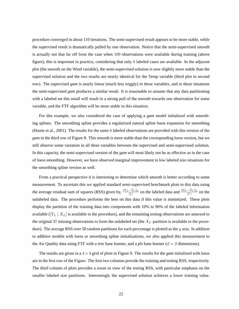
procedure converged in about 110 iterations. The semi-supervised result appears to be more stable, while

the supervised result is dramatically pulled by one observation. Notice that the semi-supervised smooth

is actually not that far off from the case when 109 observations were available during training (above

figure); this is important in practice, considering that only 8 labeled cases are available. In the adjacent

plot (the smooth on the Wind variable), the semi-supervised solution is now slightly more stable than the

supervised solution and the two results are nearly identical for the Temp variable (third plot in second

row). The supervised gam is nearly linear (much less wiggly) in these variables, and in these situations

the semi-supervised gam produces a similar result. It is reasonable to assume that any data partitioning

with a labeled set this small will result in a strong pull of the smooth towards one observation for some

variable, and the FTF algorithm will be more stable in this situation.

For this example, we also considered the case of applying a gam model initialized with smooth-

ing splines. The smoothing spline provides a regularized natural spline basis expansion for smoothing

(Hastie et al., 2001). The results for the same 8 labeled observations are provided with this version of the

gam in the third row of Figure 8. This smooth is more stable than the corresponding loess version, but we

still observe some variation in all three variables between the supervised and semi-supervised solution.

In this capacity, the semi-supervised version of the gam will most likely not be as effective as in the case

of loess smoothing. However, we have observed marginal improvement in low labeled size situations for

the smoothing spline version as well.

From a practical perspective it is interesting to determine which smooth is better according to some

measurement. To ascertain this we applied standard semi-supervised benchmark plots to this data using

the average residual sum of squares (RSS) given by, ‖YL−YL‖2

|L| on the labeled data and ‖YU−YU‖2

|U | on the

unlabeled data. The procedure performs the best on this data if this value is minimized. These plots

display the partition of the training data into components with 10% to 90% of the labeled information

available ([YL | XL] is available to the procedure), and the remaining testing observations are annexed to

the original 37 missing observations to form the unlabeled set (the XU partition is available to the proce-

dure). The average RSS over 50 random partitions for each percentage is plotted as the y axis. In addition

to additive models with loess or smoothing spline initializations, we also applied this measurement to

the Air Quality data using FTF with a tree base learner, and a pls base learner (d = 2 dimensions).

The results are given in a 4×3 grid of plots in Figure 9. The results for the gam initialized with loess

are in the first row of the Figure. The first two columns provide the training and testing RSS, respectively.

The third column of plots provides a zoom in view of the testing RSS, with particular emphasis on the

smaller labeled size partitions. Interestingly the supervised solution achieves a lower training value.

22

20 40 60 80

0.05

0.06

0.07

0.08

●

●

●

●

●

●

●

●●

●


Air Quality DataGAM (Loess d=1)

% Used

Tra

inin

g R

SS

20 40 60 80

0.0

0.5

1.0

1.5

● ● ● ● ● ● ● ● ●

●



% Used

Tes

ting

RS

S

15 20 25 30 35 40

02

46

● ● ● ● ● ● ● ●

●



% Used (Zoom In)

Tes

ting

RS

S

20 40 60 80

0.04

0.05

0.06

0.07

●

●

●

●

●

●

●●

●

●


Air Quality DataGAM (Smoothing Splines)

% Used

Tra

inin

g R

SS

20 40 60 80

0.06

0.08

0.10

0.12

0.14

●● ●

●●

●

●

●

●

●


Air Quality DataGAM (Smoothing Splines)

% Used

Tes

ting

RS

S

5 10 15 20

0.1

0.2

0.3

0.4

●

●

●● ● ● ● ● ● ●

●


Air Quality DataGAM (Smoothing Spline)

% Used (Zoom In)

Tes

ting

RS

S

20 40 60 80

0.05

0.10

0.15

0.20

●●

●●

● ● ● ● ●

●


Air Quality DataRpart

% Used

Tra

inin

g R

SS

20 40 60 80

0.08

0.10

0.12

0.14

0.16

●● ● ●

●●

●

●

●

●



% Used

Tes

ting

RS

S

5 10 15 20

0.07

50.

085

0.09

50.

105

●●

●

● ●

●●

●●

●



% Used (Zoom In)

Tes

ting

RS

S

20 40 60 80

0.05

0.10

0.15

0.20

●

●

●

●

●●

●● ●

●


Air Quality DataPLS

% Used

Tra

inin

g R

SS

20 40 60 80

0.10

0.15

0.20

● ●●

●●

●

●

●

●

●


Air Quality DataPLS

% Used

Tes

ting

RS

S

5 10 15 20

0.06

0.07

0.08

0.09

0.10

0.11

●

● ● ● ● ● ● ● ●

●


Air Quality DataPLS

% Used (Zoom In)

Tes

ting

RS

S

Figure 9: Each plot shows the average (over 50 replications) training/testing RSS as a function of the%Used cases (labeled data). Each row shows a different base learner for FTF; first row uses gam ini-tialized with loess, second row gam initialized with smoothing splines, third row uses a tree learner(implemented via rpart), and the last row the pls learner. The first column of plots provides the averagetraining RSS where the %-Used varied from 10 to 90−%. The second column depicts the correspondingtesting RSS. The third column provides a zoom-in view of the testing RSS, with the %-Used restrictedto a smaller set.

23

However, the semi-supervised solution achieves a significantly lower testing RSS for many values. As

the number of labeled data increases the differences between the two solutions decreases. This result

is consistent with the previous findings seen in Figure 8. Similarly, a gam initialized with smoothing

splines also provides similar improvements (second row of Figure 9); however, the improvement is

not as pronounced as in the loess case (middle column). The semi-supervised result for the tree also

yields improvement in testing performance for extremely low labeled partitions (third row of Figure 9).

The last learner considered for this data was partial least squares 3 in the fourth row of Figure 9. The

results suggest that the semi-supervised version of this approach does not perform well for this data. A

result of this type is consistent with the literature on semi-supervised learning where one has to match

appropriately the technique to the unlabeled data (Zhu, 2006). Overall, this data set provides evidence

that the gam and tree learners lead to improvements in performance when enhanced with unlabeled data.

3.2 Application to Pharmacology Data

The data set consists of 3925 chemical compounds on which an in-house continuous solubility screen

(the concentration to dissolve in a water/solvent mixture) was performed. The covariate information

consisted of 20 attributes that are obtained through computations, which are known to be theoretically

related to a compound’s solubility. For this data set, the value Y = 3 corresponding to 1483 compounds

in the data set indicated the compound was mostly insoluble (since measurements are not possible for

Y < 3) and similarly for the y = 60 (1100 compounds) case. Scientists and statisticians involved in

the analysis of this data set were primarily interested in applying additive models to predict compound

solubility. For this analysis we focused on the regression problem of predicting the observations whose

responses take values in the 3 < y < 60 range.

The data set was partitioned into a training/testing set as before with a varying %Used for training

purposes. This set contained all the compounds with intermediate values 3 < Y < 60. In this example

we fit generalized additive models with loess smoothing, as well as with smoothing splines. Although

the main interest is in additive models, we also provide results for regression trees.

The results are presented in the 2 × 3 grid of plots shown in Figure 10. The first plot in the first

row shows the supervised and semi-supervised gam solutions using loess smoothing. The supervised

version does not perform well in low labeled situations, and is incredible sensitive to the % of data

available for training purposes. The semi-supervised gam is more stable and in general provides lower

values for testing RSS. In the case of smoothing splines (second column of plots), the supervised gam

3The partial least squares learner was implemented with the R pls package (Wehrens and Mevik, 2006).

24

20 40 60 80

1214

1618

2022

24

●● ● ● ● ● ● ● ●

●


Solubility DataGAM (Loess d=1)

% Used

Tes

ting

RS

S

20 40 60 80

12.5

13.0

13.5

14.0

14.5

●

●

●●

●●

●●

●

●


Solubility DataGAM (Smoothing Spline)

% UsedT

estin

g R

SS

20 40 60 80

13.0

13.5

14.0

14.5

●

●

●● ●

●●

●●

●

SupervisedSemi−Supervised●


Solubility DataRpart

% Used

Tes

ting

RS

S

2 4 6 8 10

020

040

060

080

010

00

● ● ● ● ● ● ● ● ● ●

●



Solubility DataGAM (Loess d=1)

% Used (Zoom In)

Tes

ting

RS

S

2 4 6 8 10

1520

2530

●

●

●●

● ●● ● ● ●

●



Solubility DataGAM (Smoothing Spline)

% Used (Zoom In)

Tes

ting

RS

S

2 4 6 8 10

13.5

14.0

14.5

15.0

15.5

16.0

●

●

● ●●

●

●

●●

●



Solubility DataRpart

% Used (Zoom In)T

estin

g R

SS

Figure 10: Each plot shows the average (over 50 replications) testing RSS as a function of %Used cases(labeled data points) for the Solubility data set. The top row shows the result, with the %Used varyingfrom 10 to 90-%. A zoom-in view for very low %Used cases, varying from 1 to 10% of the data used fortraining purposes is shown in the bottom row. The first column shows the supervised and semi-supervisedresult for the gam learner with loess smoothing, the second column for gam with smoothing splines, andthe last column for the tree learner.

is fairly stable and the improvement for training with unlabeled data is less pronounced. Notice that in

the semi-supervised case, both the loess and the smoothing spline versions exhibit similar performance,

whereas in the supervised case these approaches perform very differently. In an extreme setting (1 to

10-% of labeled data) we observe that the semi-supervised version provides a general improvement over

the supervised version for all three procedures (second row of plots). Although the above partitions may

seem extreme, it is actually quite common practice in this field to have such a low percentage of labeled

data available.

In addition to prediction with additive models, there was also interest in a potential followup analysis

using the diagnostic tools commonly associated with this modeling technique (e.g. inference) (Hastie and

Tibshirani, 1990; Hastie et al., 2001). Interestingly, the semi-supervised gam still retains characteristics

associated with additive models, and unlabeled data could potentially influence all diagnostics associated

with it.

25

4 Concluding Remarks

In this paper, an iterative algorithm is introduced for extending supervised learners into the semi-supervised

setting and its global convergence established for the class of linear smoothers and learners that lead to

linear score functions. From the analysis, it can be seen that unlabeled observations can significantly

aid in estimating functions on data in small labeled size problems. We further provide an intuitive ex-

planation for when convergence will occur, based on the quality of the connections between labeled and

unlabeled data. The FTF algorithm can also be applied in plug-in mode, where one wishes to examine

their data using some other learner. This approach is highlighted with the semi-supervised version of a

gam in both a classification and a regression context where significant improvements are observed. The

results in this work are quite useful in many applications that involve complex data scenarios. As noted

in the introduction, the usefulness of unlabeled data is not well understood in semi-supervised learn-

ing. The proposed algorithm may serve as a platform to obtain additional insights into this important

issue. Further, there are a number of interesting theoretical questions about consistency for fixed | L | as

| U |→ ∞, a topic currently under investigation.

Acknowledgments: The authors would like to thank the Editor, Associate Editor and two anonymous

reviewers for their useful and constructive comments.

Appendix: Proofs

Proposition 1. Let S be a symmetric stochastic matrix (i.e. S1 = 1, S ≥ 0) and SUU be an irreducible

and substochastic matrix. Then, the FTF algorithm converges independent of the initialization and the

solution is given by

YU = (I − SUU )−1SULYL,

provided SUU is of full rank.

Proof. In order to have that SUU is substochastic, it suffice to have indices j, such that for every index i

we have SUL(i, j) �= 0.

Let ν be a real vector taking values in IRn−m. It is sufficient to prove the result for positive ν with

norm 1. Define Tn = SUU+S2UU+...+Sn

UUn . Since ‖ SUUν ‖1≤‖ ν ‖1 for every positive vector ν one has

‖ Sn+1UU ν ‖1≤‖ SUUTnν ‖1 for every n > 0. Choose n such that Tnν ≥ δ1 (δ exists by irreducibility of

26

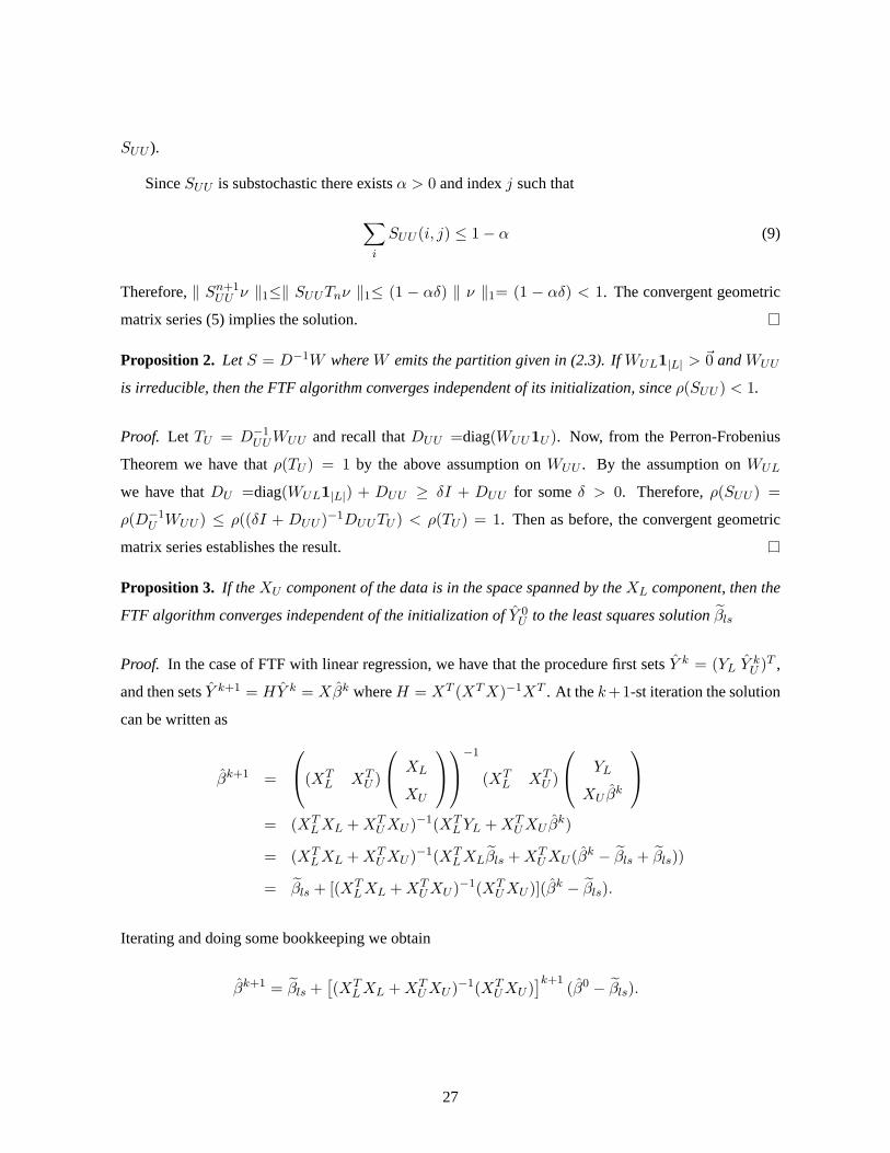
SUU ).

Since SUU is substochastic there exists α > 0 and index j such that

∑i

SUU (i, j) ≤ 1 − α (9)

Therefore, ‖ Sn+1UU ν ‖1≤‖ SUUTnν ‖1≤ (1 − αδ) ‖ ν ‖1= (1 − αδ) < 1. The convergent geometric

matrix series (5) implies the solution.

Proposition 2. Let S = D−1W where W emits the partition given in (2.3). If WUL1|L| > 0 and WUU

is irreducible, then the FTF algorithm converges independent of its initialization, since ρ(SUU ) < 1.

Proof. Let TU = D−1UUWUU and recall that DUU =diag(WUU1U ). Now, from the Perron-Frobenius

Theorem we have that ρ(TU ) = 1 by the above assumption on WUU . By the assumption on WUL

we have that DU =diag(WUL1|L|) + DUU ≥ δI + DUU for some δ > 0. Therefore, ρ(SUU ) =

ρ(D−1U WUU ) ≤ ρ((δI + DUU )−1DUUTU ) < ρ(TU ) = 1. Then as before, the convergent geometric

matrix series establishes the result.

Proposition 3. If the XU component of the data is in the space spanned by the XL component, then the

FTF algorithm converges independent of the initialization of Y 0U to the least squares solution βls

Proof. In the case of FTF with linear regression, we have that the procedure first sets Y k = (YL Y kU )T ,

and then sets Y k+1 = HY k = Xβk where H = XT (XT X)−1XT . At the k+1-st iteration the solution

can be written as

βk+1 =

⎛⎝(XT

L XTU )

⎛⎝ XL

XU

⎞⎠

⎞⎠

−1

(XTL XT

U )

⎛⎝ YL

XU βk

⎞⎠

= (XTL XL + XT

U XU )−1(XTL YL + XT

U XU βk)

= (XTL XL + XT

U XU )−1(XTL XLβls + XT

U XU (βk − βls + βls))

= βls + [(XTL XL + XT

U XU )−1(XTU XU )](βk − βls).

Iterating and doing some bookkeeping we obtain

βk+1 = βls +[(XT

L XL + XTU XU )−1(XT

U XU )]k+1

(β0 − βls).

27

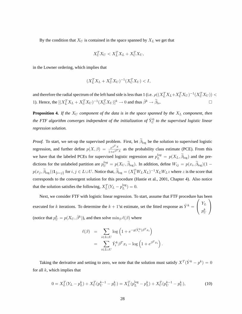
By the condition that XU is contained in the space spanned by XL we get that

XTU XU < XT

L XL + XTU XU ,

in the Lowner ordering, which implies that

(XTL XL + XT

U XU )−1(XTU XU ) < I,

and therefore the radial spectrum of the left hand side is less than 1 (i.e. ρ((XTL XL+XT

U XU )−1(XTU XU )) <

1). Hence, the [(XTL XL + XT

U XU )−1(XTU XU )]k → 0 and thus βk → βls.

Proposition 4. If the XU component of the data is in the space spanned by the XL component, then

the FTF algorithm converges independent of the initialization of Y 0U to the supervised logistic linear

regression solution.

Proof. To start, we set-up the supervised problem. First, let βlog be the solution to supervised logistic

regression, and further define p(X, β) = eβT X

1+eβT Xas the probability class estimate (PCE). From this

we have that the labeled PCEs for supervised logistic regression are plogL = p(XL, βlog) and the pre-

dictions for the unlabeled partition are plogU = p(XU , βlog). In addition, define Wij = p(xi, βlog)(1 −

p(xj , βlog))1{i=j} for i, j ∈ L∪U . Notice that, βlog = (XTL WLXL)−1XLWLz where z is the score that

corresponds to the convergent solution for this procedure (Hastie et al., 2001, Chapter 4). Also notice

that the solution satisfies the following, XTL (YL − plog

L ) = 0.

Next, we consider FTF with logistic linear regression. To start, assume that FTF procedure has been

executed for k iterations. To determine the k + 1’st estimate, set the fitted response as Y k =

⎛⎝ YL

pkU

⎞⎠

(notice that pkU = p(XU , βk)), and then solve minβ �(β) where

�(β) =∑

i∈L∪U

log(1 + e−g(Y k

i )βT xi

)

=∑

i∈L∪U

Y ki βT xi − log

(1 + eβT xi

).

Taking the derivative and setting to zero, we note that the solution must satisfy XT (Y k − pk) = 0

for all k, which implies that

0 = XTL (YL − pk

L) + XTU (pk−1

U − pkU ) = XT

L (plogL − pk

L) + XTU (pk−1

U − pkU ), (10)

28

since XTL (YL − plog

L ) = 0. Consider next, a Taylor expansion of p(X, β) about βlog, given by p(x, β) =

p(x, βlog) + ∂p(x,β)∂β (βlog)(β − βlog) + O(1). From this result, (10) becomes

XTL WLXL(βk − βlog) + XT

U WUXU (βk − βk−1) + O(1) = 0.

Rearranging terms gives

βk = (XT WX)−1(XTL WLXLβlog + XT

U WUXU βk−1) + O(1)

= βlog + [(XT WX)−1(XTU WUXU )](βk − βlog) + O(1)

Applying the same argument as with linear regression (Proposition 3) to obtain that βk+1 = βlog +

[(XT WX)−1(XTU WUXU )]k(β0 − βlog) + O(1). From the condition on XU and that plog ∈ (0, 1)|L∪U |

we have that βk −→ βlog.

References

S. Abney. Understanding the Yarowsky algorithm. Computational Linguistics, 30(3):365–395, 2004.

S. Baluja. Probabilistic modeling for face orientation discrimination: learning from labeled and unlabeled

data. In NIPS, pages 854–860, 1999.

A. Blum and S. Chawla. Learning from labeled and unlabeled data using graph mincuts. In ICML, pages

19–26, 2001.

A. Blum and T. Mitchell. Combining labeled and unlabeled data with co-training. In COLT, pages

92–100, 1998.

L. Breiman, J. Friedman, R. Olshen, and C. Stone. Classification and Regression Trees. Chapman &

Hall, New York, 1984.

A. Buja, T. Hastie, and R. Tibshirani. Linear smoothers and additive models. The Annals of Statistics,

17:543–555, 1989.

V. Castelli and T.M. Cover. The relative value of labeled and unlabeled samples in pattern recognition

with an unknown mixing parameter. IEEE Transactions on Information Theory, 42:2102–2117, 1996.

O. Chapelle, M. Chi, and A. Zien. A continuation method for semisupervised svms. In ICML, 2006a.

29

O. Chapelle, B. Scholkopf, and A. Zien, editors. Semi-Supervised Learning. MIT Press, Cambridge,

MA, 2006b. URL http://www.kyb.tuebingen.mpg.de/ssl-book.

J. Cleveland, W. Kleiner, and P. Turkey. Graphical Methods for Data Analysis. Wadsworth, 1983.

M. Culp and G. Michailidis. Graph based semi-supervised learining. IEEE Transaction on Pattern

Analysis and Machine Intelligence, 2007. To appear.

R. Duda, P. Hart, and D. Stork. Pattern Classification. Wiley, New York, NY, 2000.

R. Floyd. Algorithm 97: Shortest part. In Communications of the ACM, page 345, 1962.

T. Hastie. gam: Generalized Additive Models, 2006. R package version 0.97.

T. Hastie and R. Tibshirani. Generalized Additive Models. Chapman & Hall, CRC, Boca Raton, FL,

1990.

T. Hastie, R. Tibshirani, and J. Friedman. The Elements of Statistical Learning (Data Mining, Inference

and Prediction). Springer, New York, NY, 2001.

R. Johnson and T. Zhang. Graph-based semi-supervised learning and spectral kernel design. IEEE

Transactions on Information Theory, 2007. To appear.

R. Kondor and J. Lafferty. Diffusion kernels on graphs and other discrete input spaces. In ICML, pages

315–322, 2002.

B. Krishnapuram, D. Williams, Y. Xue, A. Hartemink, L. Carin, and M. Figueiredo. On semi-supervised

classification. In NIPS, pages 721–728, 2005.

K. Nigam, A. McCallum, S. Thrun, and T. Mitchell. Text classification from labeled and unlabeled

documents using em. Machine Learning, 39(2-3):103–134, 2000.

R Development Core Team. R: A language and environment for statistical computing. R Foundation

for Statistical Computing, Vienna, Austria, 2005. URL http://www.R-project.org. ISBN

3-900051-07-0.

B. Ripley. Pattern recognition and neural networks. Cambridge University Press, Cambrdige, UK, 1996.

T. Therneau and B. Atkinson. rpart: Recursive Partitioning, 2005. URL S-PLUS 6.x original

at http://mayoresearch.mayo.edu/mayo/research/biostat/splusfunctions.cfm.

R port by B. Ripley.

30

V. Vapnik. Statistical learning theory. Springer, New York, NY, 1998.

R. Wehrens and B. Mevik. pls: Partial Least Squares Regression (PLSR) and Principal Component

Regression (PCR), 2006. URL http://mevik.net/work/software/pls.html. R package

version 1.2-1.

T. Zhang and F. Oles. A probability analysis on the value of unlabeled data for classification problems.

In ICML, pages 1191–1198, 2000.

X. Zhu. Semi-supervised learning with graphs. Technical report, Carnegie Mellon University, Pittsburgh,

PA, 2005.

X. Zhu. Semi-supervised learning literature survey. Technical report, Computer Sciences, University of

Wisconsin-Madison, 2006.

X. Zhu and Z. Ghahramani. Learning from labeled and unabeled data with label propagation. Technical

report, Carnegie Mellon University, Pittsburgh, PA, 2002.

X. Zhu, Z. Ghahramani, and J. Lafferty. Semi-supervised learning using gaussian fields and harmonic

functions. In ICML, pages 912–919, 2003.

31

an iterative algorithm for extending learners to a semi-supervised setting

Documents