an investigation of the presence of atmospheric rivers

An Investigation of the Presence of Atmospheric Rivers over the North Pacificduring Planetary-Scale Wave Life Cycles and Their Role in Arctic Warming

CORY BAGGETT, SUKYOUNG LEE, AND STEVEN FELDSTEIN

Department of Meteorology, The Pennsylvania State University, University Park, Pennsylvania

(Manuscript received 20 January 2016, in final form 8 July 2016)

ABSTRACT

Heretofore, the tropically excited Arctic warming (TEAM) mechanism put forward that localized tropical

convection amplifies planetary-scale waves, which transport sensible and latent heat into theArctic, leading to

an enhancement of downward infrared radiation andArctic surface warming. In this study, an investigation is

made into the previously unexplored contribution of the synoptic-scale waves and their attendant atmo-

spheric rivers to the TEAMmechanism.Reanalysis data are used to conduct a suite of observational analyses,

trajectory calculations, and idealizedmodel simulations. It is shown that localized tropical convection over the

Maritime Continent precedes the peak of the planetary-scale wave life cycle by ;10–14 days. The Rossby

wave source induced by the tropical convection excites a Rossby wave train over the North Pacific that

amplifies the climatological December–March stationary waves. These amplified planetary-scale waves are

baroclinic and transport sensible and latent heat poleward. During the planetary-scale wave life cycle,

synoptic-scale waves are diverted northward over the central North Pacific. The warm conveyor belts asso-

ciated with the synoptic-scale waves channel moisture from the subtropics into atmospheric rivers that ascend

as they move poleward and penetrate into the Arctic near the Bering Strait. At this time, the synoptic-scale

waves undergo cyclonic Rossby wave breaking, which further amplifies the planetary-scale waves. The

planetary-scale wave life cycle ceases as ridging over Alaska retrogrades westward. The ridging blocks ad-

ditional moisture transport into the Arctic. However, sensible and latent heat amounts remain elevated over

the Arctic, which enhances downward infrared radiation and maintains warm surface temperatures.

1. Introduction

In our current climate, the Arctic is experiencing

warming proportionally greater than other regions of

Earth, a phenomenon known as Arctic amplification

(Serreze and Barry 2011). The consequences of a

warming Arctic and its melting sea ice are geopolitical,

biological, and meteorological—such as the opening of

shipping lanes and oil fields to exploration; the disrup-

tion of the habitats and ecosystems of native species;

and a higher frequency of atmospheric blocking and

cold-air outbreaks during winter in the midlatitudes

(Honda et al. 2009; Overland and Wang 2010; Francis

and Vavrus 2012; Liu et al. 2012). Many various mech-

anisms, ranging from atmospheric to oceanic to local

thermodynamic feedbacks, have been proposed to

explain the Arctic amplification that is currently being

observed and predicted by global climate models

(Farrell 1990; Barron et al. 1993; Cai 2006; Langen and

Alexeev 2007; Winton 2006; Sriver and Huber 2007;

Abbot and Tziperman 2008; Kump and Pollard 2008;

Walsh et al. 2008).

Apart from the above processes, an additional atmo-

spheric pathway that can produce Arctic amplification has

been proposed recently. The tropically excited Arctic

warming (TEAM) mechanism hypothesizes that localized

tropical convection near the Maritime Continent can am-

plify planetary-scale wave (PSW) activity, which leads to

enhanced poleward sensible and latent heat transports into

the Arctic. As a result of these transports, downward in-

frared radiation (IR) increases, and Arctic surface warm-

ing ensues (Doyle et al. 2011; Lee et al. 2011a,b; Yoo et al.

2011, 2012a,b; Lee 2012; Kapsch et al. 2013; Ding et al.

2014; Flournoy et al. 2016). It is important to note that the

poleward sensible and latent heat fluxes that occur when

the TEAM mechanism operates act independently of the

flux–gradient relationship of synoptic-scale baroclinic

Corresponding author address: Cory Baggett, Department of

Meteorology, The Pennsylvania State University, 503 Walker

Building, University Park, PA 16802.

E-mail: [email protected]

NOVEMBER 2016 BAGGETT ET AL . 4329

DOI: 10.1175/JAS-D-16-0033.1

� 2016 American Meteorological Society

mailto:[email protected]

waves (Lee 2014; Lee and Yoo 2014; Baggett and Lee

2015, hereafter BL15). In particular, BL15 identified

through composite analysis the existence of a PSW life

cycle (waves with zonal wavenumber k 5 1–3) that

amplifies and decays over a period of ;1–2 weeks and

manifests ;10 days after enhanced convection over the

Maritime Continent. This PSW life cycle is preceded by

an equator-to-pole temperature gradient that is very

close to its climatological value yet is followed by Arctic

warming of significant amplitude and duration. More-

over, BL15 found no evidence of enhanced, or ampli-

fied, synoptic-scale wave (SSW; k $ 4) activity during

the PSW life cycle. These characteristics of the PSW life

cycle make the TEAM mechanism a viable process for

Arctic amplification. However, the mechanism’s in-

dependence from enhanced SSW activity does not pre-

clude the possibility that the propagation of SSWs is

altered, or redirected poleward, via the influence of the

meridionally amplified planetary-scale flow present

during the PSW life cycle—a possibility we plan to ex-

plore in this study.

Recently, Woods et al. (2013) and Liu and Barnes

(2015) investigated extreme moisture intrusions into the

Arctic and their contributions to Arctic amplification.

Reminiscent of the TEAM mechanism, they found that

these intrusions are accompanied by planetary-scale, low-

frequency atmospheric patterns [or ‘‘blocks’’ (e.g.,

Henderson et al. 2016)] that can divert moisture fluxes

northward into the Arctic and thereby enhance down-

ward IR and surface warming. They showed that these

intrusions are intimately connected to SSW activity and

Rossby wave breaking, have a filamentary structure, and

rapidly convey moisture poleward, bearing a pronounced

resemblance to atmospheric rivers (ARs; Newell et al.

1992; Zhu and Newell 1998; Neiman et al. 2008; Ralph

et al. 2004; Ralph and Dettinger 2011; Newman et al.

2012; Krichak et al. 2015; Neff et al. 2014).

Although amyriad of definitions forARs exist, they are

generally characterized by having large values of total

column water (.20kgm22), being longer (.2000km)

than they are wide (,1000km), transporting moisture

poleward rapidly, and being readily identifiable with sat-

ellite imagery. Underscoring the importance of ARs to

the global water cycle and climate,Zhu andNewell (1998)

found that ARs account for a substantial majority of the

total poleward moisture transport in the midlatitudes, a

result supported by more recent studies (e.g., Guan and

Waliser 2015). Also, ARs contribute to extreme pre-

cipitation events across the world (Moore et al. 2012;

Krichak et al. 2015; De Vries et al. 2016) and have been

extensively studied for their impacts along the west coast

of North America (Higgins et al. 2000; Roberge et al.

2009; Smith et al. 2010;Neimanet al. 2011). Newmanet al.

(2012) expounded a more complex view of ARs, finding

that the moisture transport by individual events consists

of mean, low-frequency, and synoptic-scale contributions.

For example, they suggest that low-frequency tropical

forcing over the equatorial Pacific can produce an

anomalous Aleutian low that contributes to the pole-

ward moisture transport by ARs during high-frequency

synoptic-scale events. Using the algorithm created byZhu

and Newell (1998) to identify ARs [described in section

2a(3)], this study plans to explore the characteristics of

ARs entering the Arctic during the PSW life cycle.

Having identified the ARs that enter the Arctic, we

also aim to identify their moisture source regions. Sim-

ilar to prior studies that have investigated the moisture

source regions of extreme precipitation events associ-

ated with midlatitude ARs (Bao et al. 2006; Roberge

et al. 2009; Moore et al. 2012; Krichak et al. 2015; De

Vries et al. 2016), we will employ Lagrangian backward

trajectory analysis to reveal the moisture source regions

of ARs entering the Arctic. The results of these prior

analyses showed that the majority of midlatitude ARs

have moisture source regions over the subtropical and

extratropical oceanic basins as midlatitude troughs

move equatorward (Kiladis and Feldstein 1994; Ralph

et al. 2011) and converge moisture along their trailing

cold fronts. However, source regions along the northern

edge of the tropics could not be ruled out (Bao et al.

2006; Knippertz 2007; Knippertz and Wernli 2010;

Knippertz et al. 2013). Trajectory analysis also revealed

the close association of ARs to the warm conveyor belts

(Carlson 1980) of synoptic-scale cyclones (Eckhardt

et al. 2004). In fact, Bao et al. (2006) proposed that ARs

be renamed as ‘‘moisture conveyor belts.’’ More re-

cently, Dacre et al. (2015) attributed the moisture found

in ARs to local evaporation and convergence within the

warm sectors of cyclones rather than long-range transport.

Given the previously described results, we ask the

following questions. First, do SSWs and their attendant

ARs contribute to the poleward transport of moisture

into the Arctic during the PSW life cycle? Second, does

trajectory analysis reveal that the tropics serve as a

possible source region of moisture for the ARs? Third,

using an idealized model perturbed by tropical convec-

tive heating, can we reproduce the observed PSW life

cycle? Finally, how do the results of the preceding

questions modify our understanding of the TEAM

mechanism? We note here that we constrain much of

our analysis to the North Pacific while recognizing ARs

play an important role over the North Atlantic as well

(Woods et al. 2013; Liu and Barnes 2015). However, the

PSW life cycle we identify develops in response to lo-

calized tropical convection over theMaritime Continent

(Yoo et al. 2012a; BL15), and therefore the Rossby wave

4330 JOURNAL OF THE ATMOSPHER IC SC IENCES VOLUME 73

response will be most notably present in the North Pa-

cific (Sardeshmukh and Hoskins 1988).

We divide this study into two main components: an

observational analysis of reanalysis data and an initial-

value calculation using the dynamical core of a general

circulation model. Section 2 describes the data and

methods used for the observational analysis and the

model calculations, while sections 3 and 4 describe their

respective results. Section 5 concludes the paper with a

summary schematic of the PSW life cycle.

2. Data and methods

a. Observational analysis

1) DATA

For the observational component of this study, we use

daily 0000 UTC data spanning from 1979 to 2014 ob-

tained from the European Centre for Medium-Range

Weather Forecasts (ECMWF) interim reanalysis

(ERA-Interim) project (Dee et al. 2011; ECMWF2009).

We acquire the following data: zonal wind u, meridional

wind y, specific humidity q, mean sea level pressure

(MSLP), total column water (TCW), vertically in-

tegrated eastward water vapor flux Ql, vertically in-

tegrated northward water vapor flux Qu, convective

precipitation Pconv, and potential temperature u on the 2

potential vorticity unit (PVU; 1PVU5 1026Kkg21m2s21)

surface u2PVU.All of the data have a horizontal resolution of

2.58 3 2.58, while u, y, and q have an additional dimension in

the vertical consisting of 23 pressure levels.

2) SELECTION CRITERIA FOR PSW EVENTS

To identify events when the PSWs are amplified, we

integrate over the Northern Hemisphere daily values of

eddy kinetic energy (EKE) associated with k5 1–3. This

integration may be formulated as

EKE51

2

ð(u2

p 1 y2p) dm .

Here, up and yp represent the sum of the contributions of

the PSWs to u and y, respectively, found via Fourier

analysis in the longitudinal direction, and dm is an ele-

ment of atmospheric mass. Because the integrations are

performed daily, growth and decay of EKE on weekly

time scales may be used to infer PSW life cycle events

(BL15). To identify these events, we calculate anomalous

daily values of EKE by subtracting the calendar-day cli-

matology of EKE, which has had its high-frequency

variability removed by retaining only the first two har-

monics of its raw annual cycle. We first choose days

whose anomalous daily value of EKE is greater than one

standard deviation [calculated using December–March

(DJFM) daily values of EKE]. This yields 673 days, many

of which are adjacent in time to each other. Because we

are interested in identifying individual PSW life cycle

events, we next isolate the days with the greatest values of

EKE compared to the 14 calendar days both preceding

and following it. This results in no two days chosen that lie

within 14 days of each other and nets 102 PSWevents.We

perform composite analyses on all 102 events and only

the top one-third (34 events) and find both analyses to be

statistically significant and qualitatively the same. Be-

cause the composite analysis of the 34 events yields

clearer results with larger magnitudes, we choose to

present it. Finally, we note that daily anomalies of other

variables presented in the observational analysis follow

the same procedures used to find anomalous EKE.

3) DEFINITION OF Qr

During these PSW events, we diagnose the location

and direction of flow of the ARs by first objectively

identifying regions of intense moisture transport. We

adopt themathematical definition of anARproposed by

Zhu and Newell (1998) to achieve this goal. First, the

horizontal moisture flux field Qt 5 Qli 1 Qu j is parti-

tioned into the sum of two fieldsQt5Qr1Qb, whereQr

is associated with the fluxes by ARs andQb is associated

with the broad background fluxes. To construct Qr, the

magnitude of the total water vapor flux Qt at each grid

point is tested such that

Qr5

(Q

tif Q

t$Q1 0:3(Q

max2Q)

0 if Qt,Q1 0:3(Q

max2Q)

. (1)

Here, Q and Qmax are respectively the zonal mean and

max value of Qt along a given latitude circle. The

constant 0.3 is used to determine the strength of the

rivers that composeQr. Zhu and Newell (1998) tested a

range of constants from 0.1 to 0.5 and found that 0.3

gave the most reasonable separation between Qr and

Qb based on the cases they tested. In our study, we seek

to develop a qualitative picture of the location and

direction of flow of the ARs during the PSW life cycle

rather than compute their total poleward moisture

transport. To that end, we find that gently varying the

constant does not have a discernible impact on our

results. In fact, despite the somewhat arbitrary nature

of the constant employed in Eq. (1), we find our results

to be entirely consistent with recent studies that de-

veloped detection algorithms that incorporate both

integrated water vapor transport and shape criteria to

examine the anomalous frequency of occurrence of

ARs as a function of tropical convection (Guan and


Waliser 2015; Mundhenk et al. 2016). Finally, we use a

subsample of ERA-Interim data with 0.758 horizontalresolution to calculate Eq. (1) and find no discernible

difference in our results—consistent with the sensitiv-

ity tests performed by Guan and Waliser (2015).

Therefore, for the sake of computational efficiency, we

use the 2.58 horizontal resolution throughout this study.

4) BACKWARD TRAJECTORY ANALYSIS VIA

HYSPLIT

To determine the source regions of the ARs entering

the Arctic, we perform backward trajectory calculations

with the Hybrid Single-Particle Lagrangian Integrated

Trajectory (HYSPLIT; Draxler and Rolph 2015) system

of the National Oceanic and Atmospheric Administra-

tion (NOAA) Air Resources Laboratory (ARL). The

HYSPLIT system calculates the advection of parcels

using the three-dimensional wind field (u, y, and v),

which is interpolated both in time and space along the

trajectory. To perform the trajectory analysis, we em-

ploy ERA-Interim data that we format for use in the

HYSPLIT system. The formatted data have a horizontal

resolution of 2.58 by 2.58, a vertical resolution of 23

pressure levels (fully resolved between the surface and

500 hPa), and a time resolution of 6 h. We initialize

HYSPLIT during the peak intensity of the ARs and

perform backward trajectories on the parcels to de-

termine their source regions. Furthermore, we track the

following meteorological variables along each parcel’s

trajectory: pressure p, potential temperature u, equiva-

lent potential temperature uE, relative humidity, surface

precipitation rate, and surface evaporation rate.

HYSPLIT provides as direct output p, u, and relative

humidity. We acquire surface evaporation and pre-

cipitation rates from ERA-Interim and interpolate to the

parcels’ positions in time and space along their trajecto-

ries. We calculate uE according to Eq. (39) of Bolton

(1980), allowing the latent heat of vaporization to vary

as a function of air temperature. As a sensitivity test, we

also perform the trajectory analysis using the National

Centers for Environmental Prediction (NCEP)–National

Center for Atmospheric Research (NCAR) reanalysis

project (NNRP; Kalnay et al. 1996) data, which

HYSPLIT is configured to run with by default. We find

the qualitative nature of our results to be unchanged.

To choose the ARs during PSW events on which we

perform backward trajectories, we examine individually

the 34 PSWevents and pick theARwith the highest value

of Qr (the magnitude of Qr) at 658N between 1308 and2508Eduring lag days from27 through17 for each event.

This results in 32 ARs, as two of the PSW events have no

Qrwithin the aforementioned ranges. The latitude of 658Nis chosen becauseWoods et al. (2013) and Liu and Barnes

(2015) chose 708 and 608N, respectively, to identify ex-

treme moisture intrusions into the Arctic. The range of

longitudes captures the North Pacific sector. Having

identified the horizontal position and time to start each of

the 32 backward trajectories, we choose a range of starting

elevations between 100 and 10000m. Since our aim is to

determine if the intruding moisture has a tropical source

region, and knowing that parcels tend to rise along isen-

tropic surfaces, it is expected that higher, midtropospheric

elevations are more likely to reveal tropical source re-

gions. Indeed, we find that parcels starting at lower start-

ing elevations tend to intersect the surface quickly along

their backward trajectories, thereby revealing sources of

moisture at higher latitudes (Roberge et al. 2009).

b. Model calculations

To explore the importance of tropical convection in

both exciting the PSW life cycle and inducing poleward

moisture transport, we employ the spectral dynamical

core model from the NOAA Geophysical Fluid Dy-

namics Laboratory (GFDL). Our model is run for

28 days with a horizontal resolution of triangular 42

and a vertical resolution of 28 sigma s levels. The model

incorporates fourth-order horizontal diffusion with a

damping time scale of 0.1 days at its smallest scale.

Vertical diffusion is not included, but we find our results

are insensitive to its absence. The model incorporates

Newtonian cooling and Rayleigh friction, which are

precisely formulated and parameterized according to

Held and Suarez (1994).

The initial background fields for our model calcula-

tions correspond to the climatologicalDJFMvalues of u,

y, ps, q, and temperature T. Each field is derived from

the monthly means of daily means of ERA-Interim data

spanning from 1979 to 2014. Since the GFDL spectral

dynamical core is a dry model, q is utilized only as a

passive tracer qtr in order to study the influence of the

model’s evolving flow field on the redistribution of at-

mospheric water vapor. Therefore, qtr has neither dy-

namical nor thermodynamical effects on the model and

thereby does not influence the density of air, mass fluxes,

latent heat release, or any other processes that are as-

sociated with water vapor. Because the climatological

background flow fields are themselves not in a balanced

state, it is necessary to add a forcing term to the model’s

equations to prevent them from evolving (Franzke et al.

2004; Yoo et al. 2012a). To acquire this forcing term, we

initialize the model with the climatological fields and

integrate the model forward by one time step. With the

introduction of this forcing term, the modeled fields will

only evolve when a perturbation is added to the clima-

tological background fields. The perturbation we apply

to the model experiment (EXP) is the heating rate


h* (K s21) that corresponds to the latent heat release

associated with the composite of tropical convective

precipitation Pconv (m s21) during the PSW life cycle.

To create h*, we adopt the methods of Yoo et al.

(2012a), to which we refer the reader for further

details.

Because EXP uses a DJFM climatological background

flow for its initial state, there are no embedded short-

waves in the initial flow that would amplify into SSWs

through baroclinic instability and reinforce the PSW

anomaly. In fact, for such SSWs to develop, it would re-

quire the forcing in the tropics to propagate into and to

sufficiently stir the midlatitudes. Jin and Hoskins (1995)

showed in a similar model with imposed tropical heating

that it takes about two weeks for SSWs to develop

through baroclinic instability. Also, because there is no

diabatic heat release, any SSWs that develop would have

to do so in the absence of diabatic energization (Willison

et al. 2013). For these reasons, we expect that the agree-

ment between EXP and the observed PSW life cycle will

gradually deteriorate as the stirred wave propagates into

higher latitudes. Therefore, discrepancies between EXP

and PSW would augment the interpretation of the ob-

servational analyses that the SSWs play an important role

in shaping the PSWs and ARs in the extratropics.

3. Observational analysis

We begin our observational analysis with a motiva-

tional figure that displays the climatological values of

sensible and latent heat flux convergence (HFC) as

functions of k and latitude during DJFM (Fig. 1; shad-

ing). There are two distinct dipoles in sensible HFC: one

for PSWswhere k’ 1–3 and one for SSWswhere k’ 5–7

(Fig. 1a). The SSW dipole exhibits a maximum in di-

vergence at ;308N and a maximum in convergence at

;508N, while the PSW dipole resides farther north with

peak values of divergence and convergence at;458 and708N, respectively. With respect to latent HFC, there

again exists an SSW dipole (Fig. 1b). However, com-

pared to its sensible HFC counterpart, it subsumes

higher wavenumbers, reflecting the important contri-

bution by smaller-scale features in moisture transport.

The stark difference in spatial scale between the sensible

and latent heat transports can be interpreted from a

quasigeostrophic (QG) framework where temperature

can be scaled by streamfunction, which is selective to-

ward larger horizontal scales. In contrast, to the extent

that moisture may be regarded as a passive tracer field

embedded in a nonsteady flow, it is expected to undergo

chaotic filamentation (Aref 1984; Ottino 1990) and

thereby project onto smaller horizontal scales.

PSW latent HFC displays peak values of divergence

and convergence at ;108 and ;658N, respectively. Be-

tween these two centers, there appears a secondary cen-

ter of divergence at ;408N adjacent to two regions with

less clear PSW signals. From Fig. 1, it is clear that the

PSWs are instrumental in delivering heat and moisture

into the Arctic, whereas the influence of the SSWs fades

poleward of 608N. To explain this fading influence, it may

be argued that as an SSW with a conserved wavelength

propagates poleward, spherical geometry requires its k to

decrease, mathematically transforming it into a PSW.

However, if spherical geometry accounts for the re-

duction in k, one would expect the dipoles in Fig. 1 to be

FIG. 1. DJFM climatological zonal means of (a) meridional

sensible heat flux (contours; outermost contour and contour

interval are 5 3 106Wm21) and sensible HFC (shading) and

(b) meridional latent heat flux (contours; outermost contour

and contour interval are 1 3 106Wm21) and latent HFC

(shading) as functions of latitude and k. Calculated according to

2= � ðcpg21ÐvkTk dpÞ and 2= � ðLyg

21Ðvkqk dpÞ, respectively,

where vk 5 uki 1 vkj. Two iterations of nine-point local

smoothing were applied before plotting. Derived from ERA-Interim

(1979–2014) data.


tilted from left to right with decreasing latitude. For ex-

ample, if the k 5 2 sensible HFC maximum at 708Nconserved its wavelength, then the sensible HFC mini-

mum near 508N would correspond to k 5 4 or 5. The

absence of tilt for the sensible HFC dipole therefore

implies that the planetary-scale dipoles in Fig. 1 are dis-

tinct from those at the synoptic scale. In addition, using

ray tracing for a simple baroclinic model with a realistic

background flow, Hoskins and Karoly (1981) showed

that, while PSWs can propagate into theArctic, SSWs fail

to reach the Arctic as they undergo reflection equator-

ward of 608N.

In Figs. 2a and 2b, we plot composites of the zonal

means of anomalous SSW and PSW latent HFC during

the PSW life cycle. Although SSW latentHFC shows little

statistical significance, there are some signals worth

mentioning (Fig. 2a). First, near lag day 23, there is a

divergence–convergence dipole straddling ;358N. This

dipole matches the SSW climatology well (Fig. 1b) and

therefore indicates a modest enhancement of SSW ac-

tivity just before the peak of the PSW life cycle. By lag

day 0, this dipole disappears, which suggests that there is a

transfer of energy to larger scales that contributes to the

growth of the PSWs. Near lag day 0 and centered at

;458N, a new dipole with anomalous convergence (di-

vergence) to the south (north) develops and lasts;7 days.

This second dipole appears to fill a gapwith no clear signal

in PSW latentHFCnear lag day 0 at;458N(Fig. 2b). This

gap develops as a PSW divergence–convergence dipole,

which first developed near lag day 27, splits with the di-

vergence (convergence) center propagating southward

(northward). The propagation of these centers may be

explained by the growth in amplitude, and thereby me-

ridional extent, of the PSWs themselves. Furthermore, at

lag day 0, the values of anomalous PSW latent HFC show

overall agreement in sign at all latitudes with the PSW

latent HFC climatology (Fig. 1b), suggesting the PSW life

cycle reinforces the PSW climatology. Finally, Fig. 2c

shows that the anomalous TCWduring the PSW life cycle

may largely be explained in the midlatitudes and the

Arctic by the PSW latent HFC anomalies. The deficit in

TCWover the tropics reflects thatmost PSWevents occur

during La Niña conditions (Lee 2012; BL15). Most re-

markably, the positive TCW anomalies over the Arctic

begin developing near lag day25 and last more than two

weeks, indicating a prolonged period of enhanced

downward IR and surface warming.

We now investigate the presence and characteristics

of ARs over the North Pacific during the PSW life

cycle. Figures 3a and 3f collectively depict climato-

logical values of Qr frequency (the percentage of days

when Qr is nonzero), MSLP, and Qr during DJFM.

There are maxima in Qr frequency along the North

Pacific storm track, the tropical easterlies, and north of

808N because of the influence of spherical geometry on

Eq. (1). The Siberian high and Aleutian low are both

visible in the MSLP field. Encircling the Aleutian low,

along its southern and eastern peripheries, Qr trans-

ports moisture east-northeastward across the North

Pacific into the west coast of North America.

Figures 3g–j depict anomalous values of MSLP and Qr

during the PSW life cycle. Through the peak of the life

cycle, the large-scale MSLP pattern exhibits a

planetary-scale surface ridge centered over the Gulf of

Alaska with a broad surface trough over western

Russia. The ridge retrogrades westward while the

Aleutian low amplifies to the south-southwest of the

ridge. The surface winds induced by the anomalous

MSLP field divert Qr to the north and west, through

the Bering Strait into the Arctic. By lag days12–4, the

center of the anomalous surface ridge resides over the

Bering Strait and blocks any additional flow of mois-

ture into the Arctic. Figures 3b–e depict anomalous

values of Qr frequency during the PSW life cycle.

Throughout the life cycle, there are positive anomalies

ofQr frequency over the Bering Strait. When added to

the climatology, these positive anomalies imply a total

Qr frequency of;25% on any individual lag day during

the PSW life cycle. Through the peak of the life cycle,

positive anomalies develop between Hawaii and the

southern Alaskan coast while negative anomalies

manifest over the west coast of North America.

These anomalies represent a backing of the clima-

tological Qr from a southwesterly to a southerly flow,

resulting in anomalous moisture transport through

the Bering Strait into the Arctic. It is worth noting

that, on lag days 12–4, Qr frequency remains anom-

alously positive over the Arctic despite the transport

of moisture being blocked by the ridge over the Be-

ring Strait. This result coincides well with the

anomalously high TCW that persists following the

peak in the PSW life cycle (Fig. 2c). Finally, the cli-

matologicalQr reestablishes itself over the west coast

of North America, quickly following the peak of the

PSW life cycle.

To gain insight on the vertical structure of the

moisture intrusions into the Arctic during the PSW

life cycle, Fig. 4 displays a composite of the anomalous

values of total northward water vapor flux yq (shad-

ing), superimposed on the DJFM climatological

values of yq (contours). We focus on the fluxes

through 658N over the Pacific sector. Although the

greatest fluxes reside in the lower troposphere, sta-

tistically significant fluxes occur throughout the entire

troposphere near the Bering Strait during negative

lags and the peak of the life cycle. The greatest


anomalous fluxes exist to the west of the largest cli-

matological values and retrograde westward by lag

day 0 (cf. Figs. 4a,d). At positive lags, the fluxes

quickly recede toward climatological values (Fig. 4e).

These fluxes by yq are consistent with the fluxes by Qr

depicted in Fig. 3 and suggest that the anomalous

fluxes by yq are largely driven by the anomalous fluxes

by Qr. In fact, we find (not shown here) that the

FIG. 2. Composites of the zonal means of anomalous (a) shortwave latent HFC, (b) longwave latent HFC, and

(c) TCW during the PSW life cycle (n 5 34 events). Dotted areas indicate statistical significance at the 5% level,

evaluated via a Monte Carlo simulation with 1000 random samples. Derived from ERA-Interim (1979–2014) data.

Model output of the zonal means of anomalous (d) shortwave latent HFC, (e) longwave latent HFC, and (f) hqtriduring EXP. Values in (a), (b), (d), and (e) are calculated according to2= � ðLyg

21Ðvkqk dpÞ, where vk5 uki1 vkj.

In (a) and (d), k $ 4 are used, k 5 1–3 are used for (b) and (e), and qtr is substituted for q in (d) and (e). Two

iterations of nine-point local smoothing were applied before plotting.


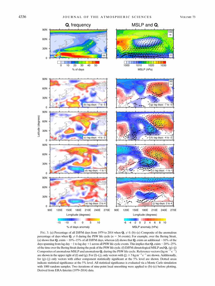
FIG. 3. (a) Percentage of all DJFM days from 1979 to 2014 when Qr 6¼ 0. (b)–(e) Composite of the anomalous

percentage of days when Qr 6¼ 0 during the PSW life cycle (n 5 34 events). For example, over the Bering Strait,

(a) shows thatQr exists;10%–15%of all DJFM days, whereas (d) shows thatQr exists an additional;10%of the

days spanning from lag day21 to lag day11 across all PSW life cycle events. This implies thatQr exists;20%–25%

of the timeover theBeringStrait during thepeakof thePSWlife cycle. (f)DJFMclimatologicalMSLPandQr. (g)–(j)

Composites of anomalousMSLP and anomalousQr during the PSW life cycle. Reference vectors (kgm21 s21)

are shown in the upper right of (f) and (g). For (f)–( j), only vectors withQr$ 5kgm21 s21 are shown.Additionally,

for (g)–( j) only vectors with either component statistically significant at the 5% level are shown. Dotted areas

indicate statistical significance at the 5% level. All statistical significance is evaluated via a Monte Carlo simulation

with 1000 random samples. Two iterations of nine-point local smoothing were applied to (b)–(e) before plotting.

Derived from ERA-Interim (1979–2014) data.


northward transport of moisture by Qr through 658Nbetween 908 and 2708E near the peak of the PSW life

cycle is essentially equal to the transport by Qt,

reaching a value of;0.713 108 kg s21. This transport is

much larger than the DJFM climatological northward

transports of ;0.24 3 108 and 0.30 3 108 kg s21 by Qr

and Qt, respectively. These values are consistent with

previous studies that find ARs account for a sub-

stantial majority of the total poleward moisture

transport in the midlatitudes (Zhu and Newell 1998;

Newman et al. 2012; Guan and Waliser 2015).

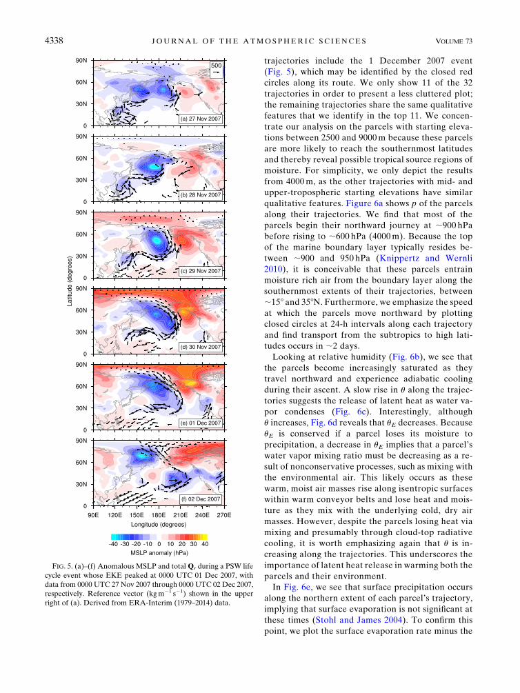
To illustrate more concretely the synoptic-scale

features that are present during the PSW life cycle,

we present a particular PSW event that peaked in

intensity on 01 December 2007. Figures 5a–f depict

anomalous MSLP and total Qr for lag days 24

through 11 during the event’s life cycle. Similar to

the composite (Fig. 3), an anomalous planetary-scale

surface ridge (trough) exists in the eastern (western)

North Pacific throughout the life cycle. This anoma-

lous MSLP pattern steers Qr northward through the

Bering Strait into the Arctic. In contrast to the com-

posite, this event shows distinct minima in MSLP,

corresponding to individual, synoptic-scale cyclones, ro-

tating through the planetary-scale trough (Figs. 5a,b,d).

These cyclones and their attendant cold fronts con-

verge and steer the low-level moisture, formingQr. In

turn, the large-scale flow and downstream blocking

steer the cyclones themselves northward. By lag

day 11 (Fig. 5f), the anomalous surface ridge has di-

minished while retrograding westward, beginning to

block any additional moisture from entering the

Arctic. However, once having entered the Arctic, Qr

is first steered westward (Fig. 5e) and then eastward

(Fig. 5f), which allows for basinwide mixing of the

warm, moisture-laden air with the cold, dry Arctic air

mass. Meanwhile, to the south of the ridge, a series of

three cyclones advances eastward toward the west

coast of North America. Finally, we note that this

event appears to have a tropical connection, with Qr

winding from the Maritime Continent and through

the Bering Strait. However, since Fig. 5 presents an

Eulerian perspective, we cannot say with certainty

that Qr transports moisture from the tropics to the

Arctic. Rather, we must employ a Lagrangian back-

ward trajectory analysis to gain insight on the path-

ways and moisture source regions of parcels entering

the Arctic.

In Fig. 6, we employ HYSPLIT to plot 11 backward

trajectories associated with ARs entering the Arctic

during the PSW life cycle. We choose the 11 with the

greatest values of Qr of the 32 ARs identified by the

algorithm presented in section 2a(4). These 11

FIG. 4. Composite of the anomalous total northward water vapor

flux yq along 658N during the PSW life cycle (shading; n 5 34

events). Black contours depict the climatological yq during DJFM.

The contour interval is 13 1023 m s21 kg kg21. Solid (dashed) lines

represent positive (negative) values; the zero contour is omitted.

Dotted areas indicate statistical significance at the 5% level, eval-

uated via a Monte Carlo simulation with 1000 random samples.

Derived from ERA-Interim (1979–2014) data.


trajectories include the 1 December 2007 event

(Fig. 5), which may be identified by the closed red

circles along its route. We only show 11 of the 32

trajectories in order to present a less cluttered plot;

the remaining trajectories share the same qualitative

features that we identify in the top 11. We concen-

trate our analysis on the parcels with starting eleva-

tions between 2500 and 9000m because these parcels

are more likely to reach the southernmost latitudes

and thereby reveal possible tropical source regions of

moisture. For simplicity, we only depict the results

from 4000m, as the other trajectories with mid- and

upper-tropospheric starting elevations have similar

qualitative features. Figure 6a shows p of the parcels

along their trajectories. We find that most of the

parcels begin their northward journey at ;900 hPa

before rising to ;600 hPa (4000m). Because the top

of the marine boundary layer typically resides be-

tween ;900 and 950 hPa (Knippertz and Wernli

2010), it is conceivable that these parcels entrain

moisture rich air from the boundary layer along the

southernmost extents of their trajectories, between

;158 and 358N. Furthermore, we emphasize the speed

at which the parcels move northward by plotting

closed circles at 24-h intervals along each trajectory

and find transport from the subtropics to high lati-

tudes occurs in ;2 days.

Looking at relative humidity (Fig. 6b), we see that

the parcels become increasingly saturated as they

travel northward and experience adiabatic cooling

during their ascent. A slow rise in u along the trajec-

tories suggests the release of latent heat as water va-

por condenses (Fig. 6c). Interestingly, although

u increases, Fig. 6d reveals that uE decreases. Because

uE is conserved if a parcel loses its moisture to

precipitation, a decrease in uE implies that a parcel’s

water vapor mixing ratio must be decreasing as a re-

sult of nonconservative processes, such as mixing with

the environmental air. This likely occurs as these

warm, moist air masses rise along isentropic surfaces

within warm conveyor belts and lose heat and mois-

ture as they mix with the underlying cold, dry air

masses. However, despite the parcels losing heat via

mixing and presumably through cloud-top radiative

cooling, it is worth emphasizing again that u is in-

creasing along the trajectories. This underscores the

importance of latent heat release in warming both the

parcels and their environment.

In Fig. 6e, we see that surface precipitation occurs

along the northern extent of each parcel’s trajectory,

implying that surface evaporation is not significant at

these times (Stohl and James 2004). To confirm this

point, we plot the surface evaporation rate minus the

FIG. 5. (a)–(f) Anomalous MSLP and totalQr during a PSW life

cycle event whose EKE peaked at 0000 UTC 01 Dec 2007, with

data from 0000 UTC 27 Nov 2007 through 0000 UTC 02 Dec 2007,

respectively. Reference vector (kgm21 s21) shown in the upper

right of (a). Derived from ERA-Interim (1979–2014) data.


surface precipitation rate (Fig. 6f) and find the pre-

ponderance of positive values exists over the sub-

tropics (white gaps in the trajectories indicate

negative values). We conclude that the most probable

moisture source for the parcels entering the Arctic

between 2500 and 9000m is the subtropics, where the

parcels are unsaturated, closest to the marine

boundary layer, and evaporation at the surface ex-

ceeds precipitation. This conclusion agrees with the

results of Gimeno et al. (2015), who identified non-

tropical source regions over the North Pacific as being

important for moisture in the Arctic over the East

Siberian Sea. Despite a probable subtropical moisture

source, we cannot dismiss the likelihood that moisture

derives from higher latitudes (Sodemann and Stohl

2013), particularly for parcels that enter the Arctic at

lower elevations. Moreover, moisture may be hori-

zontally converged into the ARs from neighboring

source regions that experience local evaporation or

from in situ convection, which is not resolved well at

ERA-Interim’s resolution. However, the decline in uEalong the trajectories suggests that the above two

processes, insomuch as they occur, are less important

than the net drying of the parcel through its mixing

with environmental air.

We now connect the results presented in this studywith

those recently presented by Woods et al. (2013) and Liu

and Barnes (2015). These studies showed that extreme

FIG. 6. Shown are 11 selected backward trajectories calculated viaHYSPLIT ofQr intrusions into theArctic during

PSW life cycle events. All trajectories are initialized at 4000m and 658N. Initial longitudes and times correspond to

a given event’s peak Qr. See section 2a(4) for additional selection criteria. Displayed along each trajectory are the

(a) pressure, (b) relative humidity, (c) u, and (d) uE of the tracked parcel. (e) Surface precipitation rate. (f) Surface

evaporation rate minus surface precipitation rate (E minus P). White segments along the trajectories in (f) indicate

negative values ofEminusP. Large black circles correspond to the location where each trajectory is initialized. Small

black circles are placed at 24-h intervals along each trajectory. Each trajectory is only plotted to the southernmost

latitude that it reaches before turning to the north again. The trajectory with red circles corresponds to the PSW life

cycle event that peaks at 0000 UTC 01 Dec 2007. Derived from ERA-Interim (1979–2014) data.


moisture intrusions into theArctic from the North Pacific

basin are associated with downstream blocking and cy-

clonicRossbywave breaking by examining fields of u2PVU.

The u2PVU surface resides very close to the tropopause in

the extratropics and may be used to diagnose Rossby

wave breaking (Franzke et al. 2011; Liu and Barnes

2015). From a potential vorticity perspective (Hoskins

et al. 1985), onewould expect Rossbywave breaking near

the tropopause to influence the MSLP field and thereby

redirect moisture transport. We tie our results to Fig. 4c

of Liu and Barnes (2015) by plotting composites of u2PVU

and anomalous Qr in Fig. 7a. Rather than compositing

these fields on lag day 0 of the PSW life cycle, we per-

form a temporal and spatial shift on each event before

compositing. We center the composite on the day that

corresponds to when the 32 ARs identified in section

2a(4) cross into the Arctic, and shift each event onto a

common longitude. Figure 7a reveals the total u2PVU

field to be nearly identical to that in Liu and Barnes

(2015). Essentially, there is a meridional overturning of

total u2PVUwith the adjacent troughs and ridges tilted in a

northwest-to-southeast fashion, indicative of cyclonic

Rossby wave breaking (Thorncroft et al. 1993; Franzke

et al. 2011). To the west-southwest of the largest positive

u2PVU anomaly, we find that Qr exhibits its largest

northward component. Furthermore, Franzke et al.

(2011) identified the importance of cyclonic Rossby wave

breaking in the building of the positive phase of the

Pacific–North America teleconnection pattern. They

found that cyclonic Rossby wave breaking in the

North Pacific was favored following enhanced

tropical convection in the western Pacific, near the

Maritime Continent. Therefore, the extreme moisture

intrusions found here and in the aforementioned studies

are likely linked to PSW dynamics where tropical

convection plays a central role in amplifying the PSWs.

We test this hypothesis using an idealized model in

section 4.

To conclude our observational analysis, we composite

and display on a skew-T diagram the vertical profiles of T,

dewpoint temperature Td, u, and y (Fig. 8). The composite

is centered in time and longitude in a manner identical to

Fig. 7a. We advise caution in interpreting the lowest levels

of the atmosphere because surface pressures at high lati-

tudes are oftentimes greater than 1000hPa. In fact, ra-

diosonde data from Arctic stations show a very complex

boundary layer, with steep, shallow inversions that lie be-

neath the 1000-hPa surface. For this reason, the planetary

boundary layer may not be accurately represented in

Fig. 8. Nevertheless, we observe several interesting fea-

tures. Beginning on lag day211we see a relatively dry and

cold troposphere with T near 2208C at 1000hPa, un-

derneath an inversion that exists up to 850hPa. The ver-

tical wind profile shows light northeasterlies near the

surface and calm winds aloft. Progressing through lag day

0, the entire troposphere warms and moistens as southerly

winds strengthen aloft and surface winds veer southeast-

erly. Indeed, the vertical wind profile veers with height,

FIG. 7. (a) Composite of total u2PVU and anomalousQr averaged from lag day21 to lag day11 ofQr intrusions

into the Arctic during PSW life cycle events (n 5 32 events). The composite is made after shifting each event in

time and longitude such that each event is centered on its peak Qr at 658N. See the section 2a(4) for additional

selection criteria. Two iterations of nine-point local smoothing were applied before plotting. Derived fromERA-

Interim (1979–2014) data. (b) Model output of total u2PVU and anomalous Qr averaged over model days 13–15

during EXP. Model output anomalous Qr is calculated by applying Eq. (1) to the model output anomalous Qt.

Reference vectors (kg m21 s21) are shown in the upper right of (a) and (b). Only vectors with Qr $ 5 kgm21 s21

and Qr $ 0.5 kgm21 s21 are shown for (a) and (b), respectively. Black contours depict anomalous u2PVU with

contour intervals of 3 and 0.3 K for (a) and (b), respectively. Solid (dashed) lines represent positive (negative)

anomalies; the zero contour is omitted.


indicative ofwarmair advection.Remarkably, on lag day 0,

T has reached 08C at 1000 hPa, while the surface in-

version has completely eroded. Furthermore, the prox-

imity of the T and Td profiles to each other suggests a

cloudy, precipitating atmosphere—a conclusion supported

by Fig. 6e. On lag day 16 (not shown here), we see the

surface inversion begin to reestablish itself, while lower-

tropospheric values of T and Td remain elevated by;28Ccompared to their values seen on lag day 26. This is

consistent with the positive TCW anomalies (Fig. 2c) and

positive 2-m temperatures (Fig. 4a of BL15) observed

following the peak of the PSW life cycle. Furthermore, the

positive T and Td anomalies, seen before and after the

moisture intrusions, contribute to enhanced downward IR

(Doyle et al. 2011;Kapsch et al. 2013; Flournoy et al. 2016).

Insomuch as basinwide mixing of the warm, moisture-

laden air with the cold, dryArctic air occurs (Figs. 2c, 5e–f,

6d), the enhanced downward IR can lead to surface

warming throughout the entire Arctic.

4. Model analysis

In this section, we perform EXP to test the hypoth-

esis that localized tropical convection can lead to the

development of PSWs that transport moisture into the

Arctic. We perturb the model with an h* that corre-

sponds to the composite of the 5-day average of

anomalous Pconv seen during the PSW life cycle,

FIG. 8. Composite skew T ofQr intrusions into the Arctic during PSW life cycle events (n532 events). The composite is made after shifting each event in time and longitude such that

each event is centered on its peak Qr at 658N. See section 2a(4) for additional selection cri-

teria. Four selected lag days are shown: 211, 26, 23, and 0 in black, blue, yellow, and red,

respectively. Solid (dashed) lines represent T (Td). Wind barbs on the right, with half lines

and full lines representing 5 and 10 m s21 intervals, respectively. Derived from ERA-Interim

(1979–2014) data.


centered on lag day212. We set h* to increase linearly

from zero to its full value on day 1, to be stationary for

the next 8 days, and to decrease linearly back to zero on

day 10. We conduct various sensitivity tests by chang-

ing the number of lag days to average, the lag day to

center the average on, and the number of days h* is

stationary. We also try varying h* to correspond with

the observed evolution of Pconv during the PSW life

cycle. We find that a large suite of the tests, whose h* is

predominantly a function of Pconv from approximately

lag day 210 to lag day 214, produce qualitatively

similar results. Thus, we choose to present here only

the model results from the parameterization of h* as

described above.

Figure 9a depicts the composite of the anomalous

300-hPa streamfunction observed from lag day 21 to

lag day11 of the PSW life cycle. We subtract the zonal

mean at each latitude to emphasize the wave structure.

A Rossby wave train is visible, arching northeastward

through the North Pacific before reaching its turn-

ing latitude over North America and returning

equatorward via the Atlantic. The net result of this

wave pattern is to constructively interfere with, and

thereby amplify, the DJFM climatological stationary

waves. Interestingly, the center of the upper-level

ridge over western Alaska resides slightly west of the

surface ridge seen in Fig. 3i, which alludes to the baro-

clinic nature of these PSWs (BL15) and their contri-

bution to poleward eddy heat flux. Moreover, the

upper-level flow shows enhanced southerly flow over

both the North Pacific and North Atlantic, an ideal

pattern for the transport of moisture into the Arctic.

Figure 9b shows EXP’s anomalous (departure from

DJFM climatology) 300-hPa streamfunction pattern,

averaged over model days 13–15, in response to h*

corresponding to the anomalous Pconv shown in Fig. 9c.

The observed and modeled 300-hPa streamfunction

patterns are remarkably similar over the North Pacific,

with pattern correlations between these two quantities

peaking at 0.44 for the entire Northern Hemisphere on

model day 13 and 0.69 for the Northern Hemisphere

between 1208 and 3008E on model day 14. The results

FIG. 9. (a) Composite of anomalous 300-hPa streamfunction averaged from lag day 21 to lag day 11 of the

PSW life cycle (n 5 34 events). (b) Model output of anomalous 300-hPa streamfunction averaged over model

days 13–15 during EXP. Zonal means of the anomalous 300-hPa streamfunction have been removed before

plotting both (a) and (b). In (a) and (b) black contours depict the climatological 300-hPa streamfunction during

DJFM. The contour interval is 15 3 106 m2 s21. Solid (dashed) lines represent negative (positive) values; the

zero contour is omitted. (c) Composite of anomalous Pconv averaged from lag day 214 to lag day 210 during

the PSW life cycle, tapered away from the equator according to a cosine squared weighting function (see

section 2b). The composite (c) is used to determine h* in EXP. Dotted areas in (a) and (c) indicate statistical

significance at the 5% level, evaluated via a Monte Carlo simulation with 1000 random samples. Two iterations

of nine-point local smoothing were applied to (c) before plotting. Derived from ERA-Interim (1979–

2014) data.


of EXP suggest that Pconv drives the development of

the PSWs. Indeed, the positive anomalies of Pconv over

the Maritime Continent are ideally located to produce

upper-level divergence that interacts with the tight

absolute vorticity gradient of the East Asian sub-

tropical jet. This interaction produces a Rossby wave

source that excites a Rossby wave train that propa-

gates northeastward and reaches the Arctic ;10 days

later (Hoskins and Karoly 1981; Sardeshmukh and

Hoskins 1988), a timing consistent with the forcing and

subsequent model response seen in EXP.

We use qtr in EXP to compute the zonal means of the

SSW latent HFC anomaly (Fig. 2d), PSW latent HFC

anomaly (Fig. 2e), and the vertically integrated tracer

anomaly hqtri (Fig. 2f) found over the 28-day model

run. Comparing these figures to their counterparts

observed during the PSW life cycle (Figs. 2a–c), we see

both similarities and differences. With respect to the

SSW latent HFC anomaly, we see themodel bears little

resemblance to the PSW life cycle composite, partic-

ularly over the midlatitudes. Indeed, the model does

not produce anomalies north of the subtropics until

near model day 14. This muted SSW activity is not

entirely unexpected for the reasons enumerated in

section 2b. Figure 7b shows additional evidence for the

absence of SSW activity in the model by revealing that

total u2PVU does not overturn as it does in observa-

tions, suggesting a lack of synoptic-scale cyclonic

Rossby wave breaking. Consequently, the u2PVU

anomalies are only slightly positive over eastern Rus-

sia and the Bering Strait in the model. Furthermore,

anomalous Qr (for a definition of anomalous Qr with

respect to EXP, see the caption to Fig. 7) is only

slightly diverted northwest in the model, with larger

anomalies directed to the west coast of NorthAmerica.

These small anomalies contrast starkly with the warm

and moist intrusion seen in observations (Fig. 7a).

Therefore, to the extent that an upscale energy cascade

amplifies the PSWs during the observed PSW life cycle,

the model’s muted SSW activity may hinder the am-

plification of PSWs.

Returning our attention to Fig. 2, we see that the

PSW latent HFC anomaly in EXP resembles the PSW

life cycle composite, with prominent convergence ex-

isting at high latitudes and divergence in the mid-

latitudes. This may be seen by comparing EXP’s

anomalies after model day 16 (Fig. 2e) with those from

the PSW life cycle between lag days 25 and 12

(Fig. 2b). Consistent with the PSW life cycle, beginning

near model day 20, the convergence–divergence dipole

appears to separate over the remainder of the model

run. However, in contrast to the PSW life cycle, the

values of convergence penetrate the Arctic more

slowly. Figure 2f shows the hqtri anomaly in the model.

Because qtr is a passive tracer, it neither condenses nor

precipitates, which makes it more analogous to TCW

than to TCW vapor in the observed atmosphere. Pos-

itive anomalies of hqtri develop over the high latitudes

several days after the peak values in the PSW latent

HFC are seen, consistent with the observed PSW life

cycle (Figs. 2b,c).

Figure 10a shows the composite of the TCWanomaly

observed for lag days from 21 to 11 of the PSW life

cycle, while Fig. 10b shows EXP’s hqtri anomaly aver-

aged over model days 13–15. Both figures also depict

total Qr stretching east-northeastward from the Mari-

time Continent. Whereas the PSW life cycle shows a

diversion of Qr to the north over the central North

Pacific, the model showsQr impinging on the west coast

of North America without any diversion northwest-

ward, despite the positive hqtri anomalies that exist

along the southern coast of Alaska. In EXP, the

positive hqtri anomalies do not penetrate the highest

latitudes, as seen in the observed TCW anomalies.

Regardless, the model result does show the importance

of tropical convection amplifying the PSWs in such a

manner as to create a large-scale pathway for the

poleward transport of moisture to high latitudes. In

fact, any SSW activity impinging on the positive hqtrianomalies in the subtropics would likely converge

moisture along their attendant frontal zones, channel-

ing moisture northward in a more direct fashion

through the Bering Strait into the Arctic, as actually

observed during the PSW life cycle.

5. Conclusions

In this study we performed both observational and

model analyses to examine the role that SSWs and ARs

play in the poleward transport of moisture into the

Arctic during the PSW life cycle. The schematic in

Fig. 11 summarizes our key findings, presented in order

of occurrence during the PSW life cycle:

1) Localized tropical convection over the Maritime

Continent exists ;10–14 days before the peak of the

PSW life cycle. The importance of this convection in

developing the PSW life cycle is confirmed with an

idealized model by perturbing a climatological DJFM

background flow with heating that corresponds to the

latent heat released by this tropical convection.

2) The upper-level divergent wind produced by the trop-

ical convection interacts with the subtropical jet exiting

Southeast Asia, producing a Rossby wave source.

3) The subsequent Rossby wave train arches north-

eastward over the North Pacific before returning


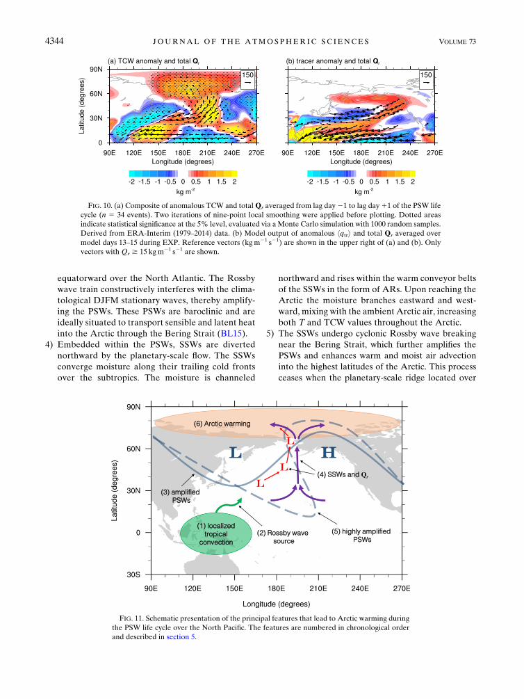
equatorward over the North Atlantic. The Rossby

wave train constructively interferes with the clima-

tological DJFM stationary waves, thereby amplify-

ing the PSWs. These PSWs are baroclinic and are

ideally situated to transport sensible and latent heat

into the Arctic through the Bering Strait (BL15).

4) Embedded within the PSWs, SSWs are diverted

northward by the planetary-scale flow. The SSWs

converge moisture along their trailing cold fronts

over the subtropics. The moisture is channeled

northward and rises within the warm conveyor belts

of the SSWs in the form of ARs. Upon reaching the

Arctic the moisture branches eastward and west-

ward, mixing with the ambient Arctic air, increasing

both T and TCW values throughout the Arctic.

5) The SSWs undergo cyclonic Rossby wave breaking

near the Bering Strait, which further amplifies the

PSWs and enhances warm and moist air advection

into the highest latitudes of the Arctic. This process

ceases when the planetary-scale ridge located over

FIG. 11. Schematic presentation of the principal features that lead to Arctic warming during

the PSW life cycle over the North Pacific. The features are numbered in chronological order

and described in section 5.

FIG. 10. (a) Composite of anomalous TCW and totalQr averaged from lag day21 to lag day11 of the PSW life

cycle (n 5 34 events). Two iterations of nine-point local smoothing were applied before plotting. Dotted areas

indicate statistical significance at the 5% level, evaluated via a Monte Carlo simulation with 1000 random samples.

Derived from ERA-Interim (1979–2014) data. (b) Model output of anomalous hqtri and total Qr averaged over

model days 13–15 during EXP. Reference vectors (kgm21 s21) are shown in the upper right of (a) and (b). Only

vectors with Qr $ 15 kgm21 s21 are shown.


Alaska retrogrades to the west, blocking any addi-

tional transport into the Arctic.

6) TCW values in the Arctic remain elevated following

the peak of the PSW life cycle. This produces

enhanced downward IR that leads to Arctic surface

warming (BL15; Flournoy et al. 2016).

With respect to the idealized model, we found that it

does not reproduce the SSW activity observed in re-

analysis data during the PSW life cycle. The lack of SSW

activity may partly be explained by the absence of dia-

batic heating through latent heat release that would

otherwise amplify the SSWs (Lackmann 2002; Grams

et al. 2011; Willison et al. 2013; Lin 2004). More im-

portantly, the model has an insufficient spinup time for

baroclinic instability to develop SSWs from a climato-

logical initial state and for the resulting SSWs to interact

with the forced PSWs. Nevertheless, the lack of SSW

activity in the model is informative because it is highly

suggestive of the importance of the SSWs in amplifying

the PSWs, which further enhances the transport of heat

and moisture to the highest latitudes—features that are

observed in reanalysis data but not in the model.

For future work, it would be beneficial to initialize the

model with daily fields rather than a climatological initial

state or to employ a fully coupled global climate model.

Presumably, the role of SSWs would be more prominent

in such experiments. Also, it would be interesting to de-

termine if the process described in Fig. 11 operates during

different seasons, such as June–August, when the sub-

tropical jet is less energized (a weakerRossby wave source)

and when low-frequency moisture transport into the Arctic

primarily derives fromcontinental source regions (Newman

et al. 2012). Finally, high-resolution regional models could

be employed to explore the sensitivity to topography of

moisture transport into theArctic.Moisture transport to the

east or west of the Bering Strait may be reduced by pre-

cipitating parcels as they ascend over high topography.

Our study offers additional insight into the TEAM

mechanism by revealing the important role that SSWs and

ARs play in warming theArctic during the PSW life cycle.

Because the PSW life cycle can contribute to Arctic am-

plification independent of the flux–gradient relationship

(BL15), we contend that the TEAMmechanism is a viable

dynamical pathway, amongst others, tomaintain a warmer

Arctic in awarmerworld (Budyko and Izrael 1991;Hoffert

and Covey 1992; Miller et al. 2010; Lee 2014). However, it

remains to be seen how much of the warming we have

observed in the Arctic is due to the TEAM mechanism

versus other processes and if the frequency of occurrence

of the PSW life cycle is dominated by natural variability or

by anthropogenic forcing—important questions that we

plan to address in future work.

Acknowledgments. This study was supported by the

National Science Foundation under Grants AGS-1139970,

AGS-1401220, and AGS-1455577. Valuable comments

from Michael Goss and George Sokolowsky helped to

improve this manuscript. All coding was performed using

the National Center for Atmospheric Research Command

Language (NCL; NCAR Command Language 2015).

REFERENCES

Abbot, D. S., and E. Tziperman, 2008: Sea ice, high-latitude con-

vection, and equable climates.Geophys. Res. Lett., 35, L03702,

doi:10.1029/2007GL032286.

Aref, H., 1984: Stirring by chaotic advection. J. Fluid Mech., 143,

1–21, doi:10.1017/S0022112084001233.

Baggett, C., and S. Lee, 2015: Arctic warming induced by tropically

forced tapping of available potential energy and the role

of the planetary-scale waves. J. Atmos. Sci., 72, 1562–1568,

doi:10.1175/JAS-D-14-0334.1.

Bao, J.-W., S. A. Michelson, P. J. Neiman, F. M. Ralph, and J. M.

Wilczak, 2006: Interpretation of enhanced integrated water

vapor bands associated with extratropical cyclones: Their

formation and connection to tropical moisture. Mon. Wea.

Rev., 134, 1063–1080, doi:10.1175/MWR3123.1.

Barron, E. J., W. H. Peterson, D. Pollard, and S. L. Thompson,

1993: Past climate and the role of ocean heat transport: Model

simulations for the Cretaceous.Paleoceanography, 8, 785–798,

doi:10.1029/93PA02227.

Bolton, D., 1980: The computation of equivalent potential

temperature. Mon. Wea. Rev., 108, 1046–1053, doi:10.1175/

1520-0493(1980)108,1046:TCOEPT.2.0.CO;2.

Budyko, M. I., and Y. A. Izrael, 1991: Anthropogenic Climate

Change. University of Arizona Press, 485 pp.

Cai, M., 2006: Dynamical greenhouse-plus feedback and polar

warming amplification. Part I: A dry radiative–transportive

climate model. Climate Dyn., 26, 661–675, doi:10.1007/

s00382-005-0104-6.

Carlson, T. N., 1980: Airflow through midlatitude cyclones and the

comma cloud pattern. Mon. Wea. Rev., 108, 1498–1509,

doi:10.1175/1520-0493(1980)108,1498:ATMCAT.2.0.CO;2.

Dacre, H. F., P. A. Clark, O. Martinez-Alvarado, M. A. Stringer, and

D.A.Lavers, 2015:Howdoatmospheric rivers form?Bull.Amer.

Meteor. Soc., 96, 1243–1255, doi:10.1175/BAMS-D-14-00031.1.

Dee, D. P., and Coauthors, 2011: The ERA-Interim reanalysis:

Configuration and performance of the data assimilation system.

Quart. J. Roy. Meteor. Soc., 137, 553–597, doi:10.1002/qj.828.De Vries, A. J., S. B. Feldstein, M. Riemer, E. Tyrlis, M. Sprenger,

M. Baumgart, M. Fnais, and J. Lelieveld, 2016: Dynamics of

tropical–extratropical interactions and extreme precipitation

events in Saudi Arabia in autumn, winter and spring. Quart.

J. Roy. Meteor. Soc., 142, 1862–1880, doi:10.1002/qj.2781.

Ding, Q., J. M. Wallace, D. S. Battisti, E. J. Steig, A. J. E. Gallant,

H.-J. Kim, and L. Geng, 2014: Tropical forcing of the recent

rapid Arctic warming in northeastern Canada and Greenland.

Nature, 509, 209–212, doi:10.1038/nature13260.

Doyle, J. G., G. Lesins, C. P. Thackray, C. Perro, G. J. Nott, T. J.

Duck, R. Damoah, and J. R. Drummond, 2011: Water vapor

intrusions into the High Arctic during winter. Geophys. Res.

Lett., 38, L12806, doi:10.1029/2011GL047493.

Draxler, R. R., and G. D. Rolph, 2015: HYSPLIT—Hybrid Single

Particle Lagrangian Integrated TrajectoryModel. NOAA/Air


http://dx.doi.org/10.1029/2007GL032286

http://dx.doi.org/10.1017/S0022112084001233

http://dx.doi.org/10.1175/JAS-D-14-0334.1

http://dx.doi.org/10.1175/MWR3123.1

http://dx.doi.org/10.1029/93PA02227

http://dx.doi.org/10.1175/1520-0493(1980)108<1046:TCOEPT>2.0.CO;2

http://dx.doi.org/10.1175/1520-0493(1980)108<1046:TCOEPT>2.0.CO;2

http://dx.doi.org/10.1007/s00382-005-0104-6

http://dx.doi.org/10.1007/s00382-005-0104-6

http://dx.doi.org/10.1175/1520-0493(1980)108<1498:ATMCAT>2.0.CO;2

http://dx.doi.org/10.1175/BAMS-D-14-00031.1

http://dx.doi.org/10.1002/qj.828


http://dx.doi.org/10.1038/nature13260

http://dx.doi.org/10.1029/2011GL047493

Resources Laboratory, 31 August 2015. [Available online at

http://ready.arl.noaa.gov/HYSPLIT.php.]

Eckhardt, S., A. Stohl, H. Wernli, P. James, C. Forster, and

N. Spichtinger, 2004: A 15-year climatology of warm

conveyor belts. J. Climate, 17, 218–237, doi:10.1175/

1520-0442(2004)017,0218:AYCOWC.2.0.CO;2.

ECMWF, 2009: The ERA-Interim project. European Centre for

Medium-Range Weather Forecasts public datasets, accessed

25 October 2013. [Available online at http://apps.ecmwf.int/

datasets/data/interim-full-daily/levtype5sfc/.]

Farrell, B. F., 1990:Equable climate dynamics. J.Atmos. Sci., 47, 2986–

2995, doi:10.1175/1520-0469(1990)047,2986:ECD.2.0.CO;2.

Flournoy, M., S. B. Feldstein, and S. Lee, 2016: Exploring the

tropically excited Arctic warming mechanism with BSRN

station data: Links between tropical convection and Arctic

downward infrared radiation. J. Atmos. Sci., 73, 1143–1158,

doi:10.1175/JAS-D-14-0271.1.

Francis, J. A., and S. J. Vavrus, 2012: Evidence linking Arctic

amplification to extreme weather in mid-latitudes. Geophys.

Res. Lett., 39, L06801, doi:10.1029/2012GL051000.

Franzke, C., S. Lee, and S. B. Feldstein, 2004: Is the North Atlantic

Oscillation a breaking wave? J. Atmos. Sci., 61, 145–160,

doi:10.1175/1520-0469(2004)061,0145:ITNAOA.2.0.CO;2.

——, S. B. Feldstein, and S. Lee, 2011: Synoptic analysis of the

Pacific–North American teleconnection pattern. Quart.

J. Roy. Meteor. Soc., 137, 329–346, doi:10.1002/qj.768.

Gimeno, L., M. Vázquez, R. Nieto, and R. M. Trigo, 2015:

Atmospheric moisture transport, the bridge between ocean

evaporation and Arctic ice melting. Earth Syst. Dyn., 6, 583–

589, doi:10.5194/esd-6-583-2015.

Grams, C. M., and Coauthors, 2011: The key role of diabatic pro-

cesses in modifying the upper-tropospheric wave guide: A

North Atlantic case-study. Quart. J. Roy. Meteor. Soc., 137,

2174–2193, doi:10.1002/qj.891.

Guan, B., andD. E.Waliser, 2015: Detection of atmospheric rivers:

Evaluation and application of an algorithm for global studies.

J. Geophys. Res. Atmos., 120, 12 514–12 535, doi:10.1002/

2015JD024257.

Held, I. M., and M. J. Suarez, 1994: A proposal for the in-

tercomparison of the dynamical cores of atmospheric general

circulation models. Bull. Amer. Meteor. Soc., 75, 1825–1830,

doi:10.1175/1520-0477(1994)075,1825:APFTIO.2.0.CO;2.

Henderson, S. A., E. D. Maloney, and E. A. Barnes, 2016: The

influence of the Madden–Julian oscillation on Northern

Hemisphere winter blocking. J. Climate, 29, 4597–4616,

doi:10.1175/JCLI-D-15-0502.1.

Higgins, R. W., J.-K. E. Schemm, W. Shi, and A. Leetmaa, 2000:

Extreme precipitation events in the western United States

related to tropical forcing. J. Climate, 13, 793–820, doi:10.1175/

1520-0442(2000)013,0793:EPEITW.2.0.CO;2.

Hoffert, M. I., and C. Covey, 1992: Deriving global climate sensi-

tivity from paleoclimate reconstructions.Nature, 360, 573–576,

doi:10.1038/360573a0.

Honda, M., J. Inoue, and S. Yamane, 2009: Influence of low Arctic

sea-ice minima on anomalously cold Eurasian winters. Geo-

phys. Res. Lett., 36, L08707, doi:10.1029/2008GL037079.

Hoskins, B. J., and D. J. Karoly, 1981: The steady linear response

of a spherical atmosphere to thermal and orographic

forcing. J. Atmos. Sci., 38, 1179–1196, doi:10.1175/

1520-0469(1981)038,1179:TSLROA.2.0.CO;2.

——, M. E. McIntyre, and A. W. Robertson, 1985: On the use and

significance of isentropic potential vorticity maps.Quart. J. Roy.

Meteor. Soc., 111, 877–946, doi:10.1002/qj.49711147002.

Jin, F., and B. J. Hoskins, 1995: The direct response to tropical

heating in a baroclinic atmosphere. J. Atmos. Sci., 52, 307–319,

doi:10.1175/1520-0469(1995)052,0307:TDRTTH.2.0.CO;2.

Kalnay, E., and Coauthors, 1996: The NCEP/NCAR 40-Year Re-

analysis Project. Bull. Amer. Meteor. Soc., 77, 437–471,

doi:10.1175/1520-0477(1996)077,0437:TNYRP.2.0.CO;2.

Kapsch, M.-L., R. G. Graversen, and M. Tjernström, 2013:

Springtime atmospheric energy transport and the control of

Arctic summer sea-ice extent. Nat. Climate Change, 3, 744–

748, doi:10.1038/nclimate1884.

Kiladis, G. N., and S. B. Feldstein, 1994: Rossby wave propagation

into the tropics in two GFDL general circulation models.

Climate Dyn., 9, 245–252, doi:10.1007/BF00208256.

Knippertz, P., 2007: Tropical–extratropical interactions related to

upper-level troughs at low latitudes. Dyn. Atmos. Oceans, 43,

36–62, doi:10.1016/j.dynatmoce.2006.06.003.

——, and H. Wernli, 2010: A Lagrangian climatology of tropical

moisture exports to the Northern Hemispheric extratropics.

J. Climate, 23, 987–1003, doi:10.1175/2009JCLI3333.1.——, ——, and G. Gläser, 2013: A global climatology of tropical

moisture exports. J. Climate, 26, 3031–3045, doi:10.1175/

JCLI-D-12-00401.1.

Krichak, S. O., J. Barkan, J. S. Breitgand, S. Gualdi, and S. B.

Feldstein, 2015: The role of the export of tropical moisture

into midlatitudes for extreme precipitation events in the

Mediterranean region. Theor. Appl. Climatol., 121, 499–515,

doi:10.1007/s00704-014-1244-6.

Kump, L. R., and D. Pollard, 2008: Amplification of Cretaceous

warmth by biological cloud feedbacks. Science, 320, 195,

doi:10.1126/science.1153883.

Lackmann, G. M., 2002: Cold-frontal potential vorticity maxima,

the low-level jet, and moisture transport in extratropical

cyclones. Mon. Wea. Rev., 130, 59–74, doi:10.1175/

1520-0493(2002)130,0059:CFPVMT.2.0.CO;2.

Langen, P. L., and V. A. Alexeev, 2007: Polar amplification as a

preferred response in an idealized aquaplanet GCM. Climate

Dyn., 29, 305–317, doi:10.1007/s00382-006-0221-x.Lee, S., 2012: Testing of the tropically excited Arctic warming

mechanism (TEAM) with traditional El Niño and La Niña.J. Climate, 25, 4015–4022, doi:10.1175/JCLI-D-12-00055.1.

——, 2014: A theory for polar amplification from a general circu-

lation perspective. Asia-Pac. J. Atmos. Sci., 50, 31–43,

doi:10.1007/s13143-014-0024-7.

——, and C. Yoo, 2014: On the causal relationship between pole-

ward heat flux and the equator-to-pole temperature gradient:

A cautionary tale. J. Climate, 27, 6519–6525, doi:10.1175/

JCLI-D-14-00236.1.

——, S. B. Feldstein, D. Pollard, and T. S. White, 2011a: Do

planetary wave dynamics contribute to equable climates?

J. Climate, 24, 2391–2404, doi:10.1175/2011JCLI3825.1.

——, T. Gong, N. Johnson, S. B. Feldstein, and D. Pollard, 2011b:

On the possible link between tropical convection and the

Northern Hemisphere Arctic surface air temperature change

between 1958 and 2001. J. Climate, 24, 4350–4367, doi:10.1175/

2011JCLI4003.1.

Lin, S. J., 2004: A ‘‘vertically Lagrangian’’ finite-volume dynamical

core for global models. Mon. Wea. Rev., 132, 2293–2307,

doi:10.1175/1520-0493(2004)132,2293:AVLFDC.2.0.CO;2.

Liu, C., and E. A. Barnes, 2015: Extreme moisture transport into

the Arctic linked to Rossby wave breaking. J. Geophys. Res.

Atmos., 120, 3774–3788, doi:10.1002/2014JD022796.

Liu, J., J. A. Curry, H. Wang, M. Song, and R. M. Horton, 2012:

Impact of declining Arctic sea ice on winter snowfall. Proc.


http://ready.arl.noaa.gov/HYSPLIT.php

http://dx.doi.org/10.1175/1520-0442(2004)017<0218:AYCOWC>2.0.CO;2

http://dx.doi.org/10.1175/1520-0442(2004)017<0218:AYCOWC>2.0.CO;2

http://apps.ecmwf.int/datasets/data/interim-full-daily/levtype=sfc/

http://apps.ecmwf.int/datasets/data/interim-full-daily/levtype=sfc/

http://dx.doi.org/10.1175/1520-0469(1990)047<2986:ECD>2.0.CO;2


http://dx.doi.org/10.1029/2012GL051000

http://dx.doi.org/10.1175/1520-0469(2004)061<0145:ITNAOA>2.0.CO;2


http://dx.doi.org/10.5194/esd-6-583-2015


http://dx.doi.org/10.1002/2015JD024257

http://dx.doi.org/10.1002/2015JD024257

http://dx.doi.org/10.1175/1520-0477(1994)075<1825:APFTIO>2.0.CO;2

http://dx.doi.org/10.1175/JCLI-D-15-0502.1

http://dx.doi.org/10.1175/1520-0442(2000)013<0793:EPEITW>2.0.CO;2

http://dx.doi.org/10.1175/1520-0442(2000)013<0793:EPEITW>2.0.CO;2

http://dx.doi.org/10.1038/360573a0

http://dx.doi.org/10.1029/2008GL037079

http://dx.doi.org/10.1175/1520-0469(1981)038<1179:TSLROA>2.0.CO;2

http://dx.doi.org/10.1175/1520-0469(1981)038<1179:TSLROA>2.0.CO;2

http://dx.doi.org/10.1002/qj.49711147002

http://dx.doi.org/10.1175/1520-0469(1995)052<0307:TDRTTH>2.0.CO;2

http://dx.doi.org/10.1175/1520-0477(1996)077<0437:TNYRP>2.0.CO;2

http://dx.doi.org/10.1038/nclimate1884

http://dx.doi.org/10.1007/BF00208256

http://dx.doi.org/10.1016/j.dynatmoce.2006.06.003

http://dx.doi.org/10.1175/2009JCLI3333.1



http://dx.doi.org/10.1007/s00704-014-1244-6

http://dx.doi.org/10.1126/science.1153883

http://dx.doi.org/10.1175/1520-0493(2002)130<0059:CFPVMT>2.0.CO;2

http://dx.doi.org/10.1175/1520-0493(2002)130<0059:CFPVMT>2.0.CO;2

http://dx.doi.org/10.1007/s00382-006-0221-x


http://dx.doi.org/10.1007/s13143-014-0024-7






http://dx.doi.org/10.1175/1520-0493(2004)132<2293:AVLFDC>2.0.CO;2

http://dx.doi.org/10.1002/2014JD022796

Natl. Acad. Sci. USA, 109, 4074–4079, doi:10.1073/

pnas.1114910109.

Miller, G. H., R. B. Alley, J. Brigham-Grette, J. J. Fitzpatrick,

L. Polyak, M. C. Serreze, and J. W. C. White, 2010: Arctic

amplification: Can the past constrain the future? Quat. Sci.

Rev., 29, 1779–1790, doi:10.1016/j.quascirev.2010.02.008.

Moore, B. J., P. J. Neiman, F. M. Ralph, and F. E. Barthold,

2012: Physical processes associated with heavy flooding

rainfall in Nashville, Tennessee, and vicinity during 1–2 May

2010: The role of an atmospheric river and mesoscale convec-

tive systems. Mon. Wea. Rev., 140, 358–378, doi:10.1175/

MWR-D-11-00126.1.

Mundhenk, B., E. A. Barnes, and E. Maloney, 2016: All-season

climatology and variability of atmospheric river frequencies

over the North Pacific. J. Climate, 29, 4885–4903, doi:10.1175/JCLI-D-15-0655.1.

NCAR Command Language, 2015: NCL version 6.3.0. UCAR/

NCAR–Computational and Information Systems Laboratory.

[Available online at http://www.ncl.ucar.edu/Download/.]

Neff, W., G. P. Compo, F. M. Ralph, and M. D. Shupe, 2014:

Continental heat anomalies and the extreme melting of the

Greenland ice surface in 2012 and 1889. J. Geophys. Res. At-

mos., 119, 6520–6536, doi:10.1002/2014JD021470.

Neiman, P. J., F. M. Ralph, G. A. Wick, J. Lundquist, and M. D.

Dettinger, 2008: Meteorological characteristics and overland

precipitation impacts of atmospheric rivers affecting the west

coast of North America based on eight years of SSM/I satellite

observations. J. Hydrometeor., 9, 22–47, doi:10.1175/

2007JHM855.1.

——, L. J. Schick, F. M. Ralph, M. Hughes, and G. A. Wick, 2011:

Flooding in western Washington: The connection to atmo-

spheric rivers. J. Hydrometeor., 12, 1337–1358, doi:10.1175/

2011JHM1358.1.

Newell, R. E., N. E. Newell, Y. Zhu, and C. Scott, 1992: Tropo-

spheric rivers?—A pilot study. Geophys. Res. Lett., 19, 2401–

2404, doi:10.1029/92GL02916.

Newman, M., G. N. Kiladis, K. M. Weickmann, F. M. Ralph, and

P. D. Sardeshmukh, 2012: Relative contributions of synoptic

and low-frequency eddies to time-mean atmospheric moisture

transport, including the role of atmospheric rivers. J. Climate,

25, 7341–7361, doi:10.1175/JCLI-D-11-00665.1.

Ottino, J., 1990: Mixing, chaotic advection, and turbulence.

Annu. Rev. Fluid Mech., 22, 207–253, doi:10.1146/

annurev.fl.22.010190.001231.

Overland, J. E., and M. Wang, 2010: Large-scale atmospheric cir-

culation changes are associated with the recent loss of Arctic

sea ice.Tellus, 62A, 1–9, doi:10.1111/j.1600-0870.2009.00421.x.

Ralph, F. M., and M. D. Dettinger, 2011: Storms, floods and the

science of atmospheric rivers. Eos, Trans. Amer. Geophys.

Union, 92, 265–272, doi:10.1029/2011EO320001.

——, P. J. Neiman, and G. A. Wick, 2004: Satellite and CALJET

aircraft observations of atmospheric rivers over the eastern

North Pacific Ocean during the winter of 1997/98. Mon. Wea.

Rev., 132, 1721–1745, doi:10.1175/1520-0493(2004)132,1721:

SACAOO.2.0.CO;2.

——, ——, G. N. Kiladis, K. Weickmann, and D. W. Reynolds,

2011: A multiscale observational case study of a Pacific at-

mospheric river exhibiting tropical–extratropical connections

and a mesoscale frontal wave. Mon. Wea. Rev., 139, 1169–

1189, doi:10.1175/2010MWR3596.1.

Roberge, A., J. R. Gyakum, and E. H. Atallah, 2009: Analysis of

intense poleward water vapor transports into high latitudes of

western North America. Wea. Forecasting, 24, 1732–1747,

doi:10.1175/2009WAF2222198.1.

Sardeshmukh, P. D., and B. J. Hoskins, 1988: The generation of

global rotational flow by steady idealized tropical di-

vergence. J. Atmos. Sci., 45, 1228–1250, doi:10.1175/

1520-0469(1988)045,1228:TGOGRF.2.0.CO;2.

Serreze, M. C., and R. G. Barry, 2011: Processes and impacts of

Arctic amplification: A research synthesis. Global Planet.

Change, 77, 85–96, doi:10.1016/j.gloplacha.2011.03.004.

Smith, B. L., S. E. Yuter, P. J. Neiman, and D. E. Kingsmill, 2010:

Water vapor fluxes and orographic precipitation over Northern

California associatedwith a landfalling atmospheric river.Mon.

Wea. Rev., 138, 74–100, doi:10.1175/2009MWR2939.1.

Sodemann, H., and A. Stohl, 2013: Moisture origin and meridional

transport in atmospheric rivers and their association with

multiple cyclones. Mon. Wea. Rev., 141, 2850–2868,

doi:10.1175/MWR-D-12-00256.1.

Sriver, R. L., and M. Huber, 2007: Observational evidence for an

ocean heat pump induced by tropical cyclones. Nature, 447,

577–580, doi:10.1038/nature05785.

Stohl, A., and P. James, 2004: A Lagrangian analysis of the atmo-

spheric branch of the global water cycle. Part I: Method de-

scription, validation, and demonstration for the August 2002

flooding in central Europe. J. Hydrometeor., 5, 656–678,

doi:10.1175/1525-7541(2004)005,0656:ALAOTA.2.0.CO;2.

Thorncroft, C. D., B. J. Hoskins, and M. E. McIntyre, 1993: Two

paradigms of baroclinic-wave life-cycle behaviour. Quart.

J. Roy. Meteor. Soc., 119, 17–55, doi:10.1002/qj.49711950903.Walsh, J. E., W. L. Chapman, V. Romanovsky, J. H. Christensen,

andM. Stendel, 2008: Global climate model performance over

Alaska and Greenland. J. Climate, 21, 6156–6174, doi:10.1175/

2008JCLI2163.1.

Willison, J., W. A. Robinson, and G. M. Lackmann, 2013: The

importance of resolving mesoscale latent heating in the North

Atlantic storm track. J. Atmos. Sci., 70, 2234–2250,

doi:10.1175/JAS-D-12-0226.1.

Winton, M., 2006: Amplified Arctic climate change: What does

surface albedo feedback have to do with it? Geophys. Res.

Lett., 33, L03701, doi:10.1029/2005GL025244.

Woods, C., R. Caballero, and G. Svensson, 2013: Large-scale cir-

culation associated with moisture intrusions into the Arctic

during winter.Geophys. Res. Lett., 40, 4717–4721, doi:10.1002/

grl.50912.

Yoo, C., S. B. Feldstein, and S. Lee, 2011: The impact of the

Madden–Julian Oscillation trend on the Arctic amplification

of surface air temperature during the 1979–2008 boreal winter.

Geophys. Res. Lett., 38, L24804, doi:10.1029/2011GL049881.

——, S. Lee, and S. B. Feldstein, 2012a:Arctic response to anMJO-

like tropical heating in an idealized GCM. J. Atmos. Sci., 69,

2379–2393, doi:10.1175/JAS-D-11-0261.1.

——, ——, and ——, 2012b: Mechanisms of extratropical sur-

face air temperature change in response to the Madden–

Julian oscillation. J. Climate, 25, 5777–5790, doi:10.1175/

JCLI-D-11-00566.1.

Zhu, Y., and R. E. Newell, 1998: A proposed algorithm for moisture

fluxes from atmospheric rivers. Mon. Wea. Rev., 126, 725–735,

doi:10.1175/1520-0493(1998)126,0725:APAFMF.2.0.CO;2.


http://dx.doi.org/10.1073/pnas.1114910109

http://dx.doi.org/10.1073/pnas.1114910109

http://dx.doi.org/10.1016/j.quascirev.2010.02.008

http://dx.doi.org/10.1175/MWR-D-11-00126.1




http://www.ncl.ucar.edu/Download/

http://dx.doi.org/10.1002/2014JD021470

http://dx.doi.org/10.1175/2007JHM855.1




http://dx.doi.org/10.1029/92GL02916


http://dx.doi.org/10.1146/annurev.fl.22.010190.001231

http://dx.doi.org/10.1146/annurev.fl.22.010190.001231

http://dx.doi.org/10.1111/j.1600-0870.2009.00421.x

http://dx.doi.org/10.1029/2011EO320001

http://dx.doi.org/10.1175/1520-0493(2004)132<1721:SACAOO>2.0.CO;2

http://dx.doi.org/10.1175/1520-0493(2004)132<1721:SACAOO>2.0.CO;2

http://dx.doi.org/10.1175/2010MWR3596.1

http://dx.doi.org/10.1175/2009WAF2222198.1

http://dx.doi.org/10.1175/1520-0469(1988)045<1228:TGOGRF>2.0.CO;2

http://dx.doi.org/10.1175/1520-0469(1988)045<1228:TGOGRF>2.0.CO;2

http://dx.doi.org/10.1016/j.gloplacha.2011.03.004

http://dx.doi.org/10.1175/2009MWR2939.1


http://dx.doi.org/10.1038/nature05785

http://dx.doi.org/10.1175/1525-7541(2004)005<0656:ALAOTA>2.0.CO;2

http://dx.doi.org/10.1002/qj.49711950903




http://dx.doi.org/10.1029/2005GL025244

http://dx.doi.org/10.1002/grl.50912

http://dx.doi.org/10.1002/grl.50912

http://dx.doi.org/10.1029/2011GL049881




http://dx.doi.org/10.1175/1520-0493(1998)126<0725:APAFMF>2.0.CO;2

an investigation of the presence of atmospheric rivers

Documents