an intuitive introduction for understanding and … · an intuitive introduction for understanding...
TRANSCRIPT
An Intuitive Introduction For Understanding and Solving
Stochastic Differential Equations
Chris Rackauckas
June 13, 2014
Abstract
Stochastic differential equations (SDEs) are a generalization of deterministic differentialequations that incorporate a “noise term”. These equations can be useful in many applicationswhere we assume that there are deterministic changes combined with noisy fluctuations. Ito’sCalculus is the mathematics for handling such equations. In this article we introduce stochasticdifferential equations and Ito’s calculus from an intuitive point of view, building the ideas fromrelatable probability theory and only straying into measure-theoretic probability (defining allconcepts along the way) as necessary. All of the proofs are discussed intuitively and rigorously:step by step proofs are provided. . We start by reviewing the relevant probability needed inorder to develop the stochastic processes. We then develop the mathematics of stochastic pro-cesses in order to define the Poisson Counter Process. We then define Brownian Motion, orthe Wiener Process, as a limit of the Poisson Counter Process. By doing the definition in thismanner, we are able to solve for many of the major properties and theorems of the stochasticcalculus without resorting to measure-theoretic approaches. Along the way, examples are givento show how the calculus is actually used to solve problems. After developing Ito’s calculus forsolving SDEs, we briefly discuss how these SDEs can be computationally simulated in case theanalytical solutions are difficult or impossible. After this, we turn to defining some relevantterms in measure-theoretic probability in order to develop ideas such as conditional expectationand martingales. The conclusion to this article is a set of four applications. We show how therules of the stochastic calculus and some basic martingale theory can be applied to solve prob-lems such as option pricing, genetic drift, stochastic control, and stochastic filtering. The endof this article is a cheat sheet that details the fundamental rules for “doing” Ito’s calculus, likeone would find on the cover flap of a calculus book. These are the equations/properties/rulesthat one rules to solve stochastic differential equations that are explained and justified in thearticle but put together for convenience.
Contents
1 Introduction 51.1 Outline . . . . . . . . . . . . . . . . . . . . . . . . . . . . . . . . . . . . . . . . . . . 5
1
2 Probability Review 62.1 Discrete Random Variables . . . . . . . . . . . . . . . . . . . . . . . . . . . . . . . . 6
2.1.1 Example 1: Bernoulli Trial . . . . . . . . . . . . . . . . . . . . . . . . . . . . 62.1.2 Example 2: Binomial Random Variable . . . . . . . . . . . . . . . . . . . . . 7
2.2 Probability Generating Functions. . . . . . . . . . . . . . . . . . . . . . . . . . . . . 82.3 Moment Generating Functions . . . . . . . . . . . . . . . . . . . . . . . . . . . . . . 92.4 Continuous Time Discrete Space Random Variables . . . . . . . . . . . . . . . . . . . 10
2.4.1 The Poisson Distribution . . . . . . . . . . . . . . . . . . . . . . . . . . . . . 112.5 Continuous Random Variables . . . . . . . . . . . . . . . . . . . . . . . . . . . . . . . 12
2.5.1 The Gaussian Distribution . . . . . . . . . . . . . . . . . . . . . . . . . . . . 122.5.2 Generalization: The Multivariate Gaussian Distribution . . . . . . . . . . . . 132.5.3 Gaussian in the Correlation-Free Coordinate System . . . . . . . . . . . . . . 14
2.6 Gaussian Distribution in PDEs . . . . . . . . . . . . . . . . . . . . . . . . . . . . . . 142.7 Independence . . . . . . . . . . . . . . . . . . . . . . . . . . . . . . . . . . . . . . . . 152.8 Conditional Probability . . . . . . . . . . . . . . . . . . . . . . . . . . . . . . . . . . 152.9 Change of Random Variables . . . . . . . . . . . . . . . . . . . . . . . . . . . . . . . 16
2.9.1 Multivariate Changes . . . . . . . . . . . . . . . . . . . . . . . . . . . . . . . 162.10 Empirical Estimation of Densities . . . . . . . . . . . . . . . . . . . . . . . . . . . . . 17
3 Introduction to Stochastic Processes: Jump Processes 173.1 Stochastic Processes . . . . . . . . . . . . . . . . . . . . . . . . . . . . . . . . . . . . 173.2 The Poisson Counter . . . . . . . . . . . . . . . . . . . . . . . . . . . . . . . . . . . . 183.3 Markov Process . . . . . . . . . . . . . . . . . . . . . . . . . . . . . . . . . . . . . . . 183.4 Time Evolution of Poisson Counter . . . . . . . . . . . . . . . . . . . . . . . . . . . . 183.5 Bidirectional Poisson Counter . . . . . . . . . . . . . . . . . . . . . . . . . . . . . . . 193.6 Discrete-Time Discrete-Space Markov Process . . . . . . . . . . . . . . . . . . . . . . 213.7 Continuous-Time Discrete-Space Markov Chain . . . . . . . . . . . . . . . . . . . . . 22
3.7.1 Example: DNA Mutations . . . . . . . . . . . . . . . . . . . . . . . . . . . . . 233.8 The Differential Poisson Counting Process and the Stochastic Integral . . . . . . . . 233.9 Generalized Poisson Counting Processes . . . . . . . . . . . . . . . . . . . . . . . . . 243.10 Important Note: The Defining Feature of Ito’s Calculus . . . . . . . . . . . . . . . . 253.11 Example Counting Process . . . . . . . . . . . . . . . . . . . . . . . . . . . . . . . . 263.12 Ito’s Rules for Poisson Jump Process . . . . . . . . . . . . . . . . . . . . . . . . . . . 26
3.12.1 Example Problem . . . . . . . . . . . . . . . . . . . . . . . . . . . . . . . . . 273.13 Dealing with Expectations of Poisson Counter SDEs . . . . . . . . . . . . . . . . . . 27
3.13.1 Example Calculations . . . . . . . . . . . . . . . . . . . . . . . . . . . . . . . 283.13.2 Another Example Calculation . . . . . . . . . . . . . . . . . . . . . . . . . . . 293.13.3 Important Example: Bidirectional Poisson Counter . . . . . . . . . . . . . . . 29
3.14 Poisson Jump Process Kolmogorov Forward Equation . . . . . . . . . . . . . . . . . 303.14.1 Example Kolmogorov Calculation . . . . . . . . . . . . . . . . . . . . . . . . 32
2
4 Introduction to Stochastic Processes: Brownian Motion 334.1 Brownian Motion / The Wiener Process . . . . . . . . . . . . . . . . . . . . . . . . . 334.2 Understanding the Wiener Process . . . . . . . . . . . . . . . . . . . . . . . . . . . . 334.3 Ito’s Rules for Wiener Processes . . . . . . . . . . . . . . . . . . . . . . . . . . . . . 344.4 A Heuristic Way of Looking at Ito’s Rules . . . . . . . . . . . . . . . . . . . . . . . . 374.5 Wiener Process Calculus Summarized . . . . . . . . . . . . . . . . . . . . . . . . . . 38
4.5.1 Example Problem: Geometric Brownian Motion . . . . . . . . . . . . . . . . 394.6 Kolmogorov Forward Equation Derivation . . . . . . . . . . . . . . . . . . . . . . . . 40
4.6.1 Example Application: Ornstein–Uhlenbeck Process . . . . . . . . . . . . . . . 424.7 Stochastic Stability . . . . . . . . . . . . . . . . . . . . . . . . . . . . . . . . . . . . . 424.8 Fluctuation-Dissipation Theorem . . . . . . . . . . . . . . . . . . . . . . . . . . . . . 43
5 Computational Simulation of SDEs 445.1 The Stochastic Euler Method - Euler-Maruyama Method . . . . . . . . . . . . . . . 445.2 A Quick Look at Accuracy . . . . . . . . . . . . . . . . . . . . . . . . . . . . . . . . 455.3 Milstein’s Method . . . . . . . . . . . . . . . . . . . . . . . . . . . . . . . . . . . . . 465.4 KPS Method . . . . . . . . . . . . . . . . . . . . . . . . . . . . . . . . . . . . . . . . 465.5 Simulation Via Probability Density Functions . . . . . . . . . . . . . . . . . . . . . . 47
6 Measure-Theoretic Probability for SDE Applications 486.1 Probability Spaces and σ-algebras . . . . . . . . . . . . . . . . . . . . . . . . . . . . 48
6.1.1 Example: Uniform Measure . . . . . . . . . . . . . . . . . . . . . . . . . . . . 496.1.2 Coin Toss Example . . . . . . . . . . . . . . . . . . . . . . . . . . . . . . . . . 49
6.2 Random Variables and Expectation . . . . . . . . . . . . . . . . . . . . . . . . . . . . 506.2.1 Example: Coin Toss Experiment . . . . . . . . . . . . . . . . . . . . . . . . . 516.2.2 Example: Uniform Random Variable . . . . . . . . . . . . . . . . . . . . . . . 516.2.3 Expectation of a Random Variable . . . . . . . . . . . . . . . . . . . . . . . . 526.2.4 Properties of Expectations: . . . . . . . . . . . . . . . . . . . . . . . . . . . . 536.2.5 Convergence of Expectation . . . . . . . . . . . . . . . . . . . . . . . . . . . . 536.2.6 Convergence Theorems . . . . . . . . . . . . . . . . . . . . . . . . . . . . . . . 53
6.3 Filtrations, Conditional Expectations, and Martingales . . . . . . . . . . . . . . . . . 546.3.1 Filtration Definitions . . . . . . . . . . . . . . . . . . . . . . . . . . . . . . . . 546.3.2 Independence . . . . . . . . . . . . . . . . . . . . . . . . . . . . . . . . . . . . 556.3.3 Conditional Expectation . . . . . . . . . . . . . . . . . . . . . . . . . . . . . . 556.3.4 Properties of Conditional Expectation . . . . . . . . . . . . . . . . . . . . . . 556.3.5 Example: Infinite Coin-Flipping Experiment . . . . . . . . . . . . . . . . . . 56
6.4 Martingales . . . . . . . . . . . . . . . . . . . . . . . . . . . . . . . . . . . . . . . . . 576.4.1 Example: Infinite Coin-Flipping Experiment Martingale Properties . . . . . . 576.4.2 Example: Brownian Motion . . . . . . . . . . . . . . . . . . . . . . . . . . . . 58
6.5 Martingale SDEs . . . . . . . . . . . . . . . . . . . . . . . . . . . . . . . . . . . . . . 586.5.1 Example: Geometric Brownian Motion . . . . . . . . . . . . . . . . . . . . . . 58
3
6.6 Application of Martingale Theory: First-Passage Time Theory . . . . . . . . . . . . 596.6.1 Kolmogorov Solution to First-Passage Time . . . . . . . . . . . . . . . . . . 596.6.2 Stopping Processes . . . . . . . . . . . . . . . . . . . . . . . . . . . . . . . . . 596.6.3 Reflection Principle . . . . . . . . . . . . . . . . . . . . . . . . . . . . . . . . 60
6.7 Levy Theorem . . . . . . . . . . . . . . . . . . . . . . . . . . . . . . . . . . . . . . . 616.8 Markov Processes and the Backward Kolmogorov Equation . . . . . . . . . . . . . . 61
6.8.1 Markov Processes . . . . . . . . . . . . . . . . . . . . . . . . . . . . . . . . . . 616.8.2 Martingales by Markov Processes . . . . . . . . . . . . . . . . . . . . . . . . 616.8.3 Transition Densities and the Backward Kolmogorov . . . . . . . . . . . . . . 62
6.9 Change of Measure . . . . . . . . . . . . . . . . . . . . . . . . . . . . . . . . . . . . . 636.9.1 Definition of Change of Measure . . . . . . . . . . . . . . . . . . . . . . . . . 636.9.2 Simple Change of Measure Example . . . . . . . . . . . . . . . . . . . . . . . 636.9.3 Radon-Nikodym Derivative Process . . . . . . . . . . . . . . . . . . . . . . . 646.9.4 Girsanov Theorem . . . . . . . . . . . . . . . . . . . . . . . . . . . . . . . . . 64
7 Applications of SDEs 667.1 European Call Options . . . . . . . . . . . . . . . . . . . . . . . . . . . . . . . . . . . 66
7.1.1 Solution Technique: Self-Financing Portfolio . . . . . . . . . . . . . . . . . . 667.1.2 Solution Technique: Conditional Expectation . . . . . . . . . . . . . . . . . . 687.1.3 Justification of µ = r via Girsanov Theorem . . . . . . . . . . . . . . . . . . . 69
7.2 Population Genetics . . . . . . . . . . . . . . . . . . . . . . . . . . . . . . . . . . . . 707.2.1 Definitions from Biology . . . . . . . . . . . . . . . . . . . . . . . . . . . . . . 707.2.2 Introduction to Genetic Drift and the Wright-Fisher Model . . . . . . . . . . 707.2.3 Formalization of the Wright-Fisher Model . . . . . . . . . . . . . . . . . . . . 717.2.4 The Diffusion Generator . . . . . . . . . . . . . . . . . . . . . . . . . . . . . . 727.2.5 SDE Approximation of the Wright-Fisher Model . . . . . . . . . . . . . . . . 737.2.6 Extensions to the Wright-Fisher Model: Selection . . . . . . . . . . . . . . . . 737.2.7 Extensions to the Wright-Fisher Model: Mutation . . . . . . . . . . . . . . . 747.2.8 Hitting Probability (Without Mutation) . . . . . . . . . . . . . . . . . . . . . 747.2.9 Understanding Using Kolmogorov . . . . . . . . . . . . . . . . . . . . . . . . 76
7.3 Stochastic Control . . . . . . . . . . . . . . . . . . . . . . . . . . . . . . . . . . . . . 767.3.1 Deterministic Optimal Control . . . . . . . . . . . . . . . . . . . . . . . . . . 767.3.2 Dynamic Programming . . . . . . . . . . . . . . . . . . . . . . . . . . . . . . 777.3.3 Stochastic Optimal Control . . . . . . . . . . . . . . . . . . . . . . . . . . . . 787.3.4 Example: Linear Stochastic Control . . . . . . . . . . . . . . . . . . . . . . . 79
7.4 Stochastic Filtering . . . . . . . . . . . . . . . . . . . . . . . . . . . . . . . . . . . . . 807.4.1 The Best Estimate: E [Xt|Gt] . . . . . . . . . . . . . . . . . . . . . . . . . . . 807.4.2 Linear Filtering Problem . . . . . . . . . . . . . . . . . . . . . . . . . . . . . 82
7.5 Discussion About the Kalman-Bucy Filter . . . . . . . . . . . . . . . . . . . . . . . . 84
8 Stochastic Calculus Cheat-Sheet 86
4
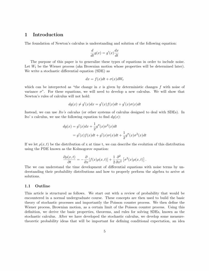
1 Introduction
The foundation of Newton’s calculus is understanding and solution of the following equation:
d
dtg(x) = g′(x)
dx
dt
The purpose of this paper is to generalize these types of equations in order to include noise.Let Wt be the Wiener process (aka Brownian motion whose properties will be determined later).We write a stochastic differential equation (SDE) as
dx = f(x)dt+ σ(x)dWt
which can be interpreted as “the change in x is given by deterministic changes f with noise ofvariance σ”. For these equations, we will need to develop a new calculus. We will show thatNewton’s rules of calculus will not hold:
dg(x) 6= g′(x)dx = g′(x)f(x)dt+ g′(x)σ(x)dt
Instead, we can use Ito’s calculus (or other systems of calculus designed to deal with SDEs). InIto’ s calculus, we use the following equation to find dg(x):
dg(x) = g′(x)dx+1
2g′′(x)σ2(x)dt
= g′(x)f(x)dt+ g′(x)σ(x)dt+1
2g′′(x)σ2(x)dt
If we let ρ(x, t) be the distribution of x at time t, we can describe the evolution of this distributionusing the PDE known as the Kolmogorov equation:
∂ρ(x, t)
∂t= − ∂
∂x[f(x)ρ(x, t)] +
1
2
∂2
∂x2
[σ2(x)ρ(x, t)
].
The we can understand the time development of differential equations with noise terms by un-derstanding their probability distributions and how to properly perform the algebra to arrive atsolutions.
1.1 Outline
This article is structured as follows. We start out with a review of probability that would beencountered in a normal undergraduate course. These concepts are then used to build the basictheory of stochastic processes and importantly the Poisson counter process. We then define theWiener process, Brownian motion, as a certain limit of the Poisson counter process. Using thisdefinition, we derive the basic properties, theorems, and rules for solving SDEs, known as thestochastic calculus. After we have developed the stochastic calculus, we develop some measure-theoretic probability ideas that will be important for defining conditional expectation, an idea
5
central to fucture estimation of stochastic processes and martingales. These properties are thenapplied to systems that may be of interest to the stochastic modeler. The first of which is theEuropean option market where we use our tools to derive the Black-Scholes equation. Next wedabble in some continuous probability models for population genetics. Lastly, we look at stochasticcontrol and filtering problems that are central to engineering and many other disciplines.
2 Probability Review
This chapter is a review of probability concepts from an undergraduate probability course. Theseideas will be useful when doing the calculations for the stochastic calculus. If you feel as thoughyou may need to review some probability before continuing, we recommend Durrett’s ElementaryProbability for Applications, or at a slightly higher level which is more mathematical, Grinsteadand Snell’s Introduction to Probability. Although a full grasp of probability is not required, it isrecommended that you are comfortable with most of the concepts introduced in this chapter.
2.1 Discrete Random Variables
2.1.1 Example 1: Bernoulli Trial
A Bernoulli trial describes the experiment of a single coin toss. There are two possible outcomesin a Bernoulli trial: the coin can land on heads or it can land on tails. We can describe this usingS, the set of all possible outcomes:
S = H,TLet the probability of the coin landing on heads be Pr(H) = p. Then, the probability of the coinlanding on tails is Pr(T ) = 1 − p . LetX be a random variable. This is a “function” that mapsS → R. It describes the values associated with each possible outcome of the experiment. Forexample, let X = 1 if we get heads, and X = 0 if we get tails, then
X(ω) =
1 if ω = H0 if ω = T
We defineE [X] as the mean of X, or the expectation of X. To find E [X], we take all the possiblevalues of X and weight them by the probability of X taking each of these values. So, for theBernoulli trial:
E [X] = Pr(H) · 1 + Pr(T ) · 0= p
We use the probability distribution of X to describe all the probabilities of X taking each of itsvalues. There are only two possible outcomes in the Bernoulli trial and thus we can write theprobability distribution as
P (X = 1) = P (H) = p
P (X = 0) = P (T ) = 1− p.
6
Define V [X] as the variance of X. This is a measure of how much the values of X diverge fromthe expectation of X on average and is defined as
V [X] = σ2x = E
[(X − E [X])2
]= E
[X2]− E [X]2 .
For the Bernoulli Trial, we get that
V [X] = E[(X − p)2
]= Pr(X = 1)(1− p)2 + Pr(X = 0)(0− p)2
= p(1− p)
2.1.2 Example 2: Binomial Random Variable
This describes an experiment where we toss a coin n times. That is, it is a Bernoulli trial repeatedn times. Each toss/repetition is assumed to be independent. The set of all possible outcomesincludes every possible sequence of heads and tails:
S = HH · · ·H,TT · · ·T,HTHTT · · · , ...
or equivalentlyS = H,Tn
We may want to describe the how large the set S is, or the cardinality of the set S, represented by|S|, as the “number of things in S”. For this example:
|S| = 2n
For each particular string of heads and tails, since each coin flip is independent, we can calculatethe probability of obtaining that particular string as
Pr(s ∈ S) = pk(1− p)n−k,where kis the number of heads in s
So for instance, P (HH · · ·H) = pn. Say we want to talk about the probability of getting a certainnumber of heads in this experiment. Then let X be the random variable for the number of heads.We can describe the range(X) as the possible values that X can take: X ∈ 0, 1, 2, ..., n. Note:using “∈” is an abuse of notation since X is actually a function. Recall that the probabilitydistribution of X is
Pr(X = k) =
(n
k
)pk(1− p)n−k
Using this probability distribution, we can calculate the expectation and variance of X. Theexpectation is
E [X] = µx =
n∑k=0
Pr(X = k) · k =
n∑k=0
(n
k
)pk(1− p)n−k · k
= n · p,
7
while the variance is
V [X] = E[(X − p)2
]=
n∑k=0
Pr(X = k)(k − np)2
= n · p(1− p).
This is all solved using the Binomial theorem:
(a+ b)n =∑k
(n
k
)akbn−k.
Note that if Xi is the Bernoulli random variable associated with the ith coin toss, then
X =
n∑i=1
Xi.
Using these indicator variables we can compute the expectation and variance for the Binomial trialmore quickly. In order to do so, we use the following facts
E [aX + bY ] = aE [X] + bE [Y ]
andV [aX + bY ] = a2V [X] + b2V [Y ] if X,Y are independent
to easily compute
E [X] =n∑i=1
E [Xi] =n∑i=1
p = np
and
V [X] =
n∑i=1
V [Xi] =
n∑i=1
p(1− p) = np(1− p)
2.2 Probability Generating Functions.
A probability function G(z) is a power series that can be used to determine the probability distri-bution of a random variable X. We define G(z) as
G(z)def= E
[zX].
For example, the Bernoulli random variable has the generating function
G(z) = E[zX]
= Pr(X = 1)z1 + Pr(X = 0)z0
= pz + (1− p)
8
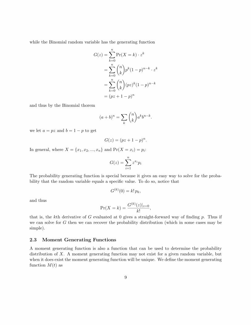
while the Binomial random variable has the generating function
G(z) =
n∑k=0
Pr(X = k) · zk
=
n∑k=0
(n
k
)pk(1− p)n−k · zk
=
n∑k=0
(n
k
)(pz)k(1− p)n−k
= (pz + 1− p)n
and thus by the Binomial thorem
(a+ b)n =∑k
(n
k
)akbn−k.
we let a = pz and b = 1− p to get
G(z) = (pz + 1− p)n.
In general, where X = x1, x2, ..., xn and Pr(X = xi) = pi:
G(z) =n∑i=1
zxipi
The probability generating function is special because it gives an easy way to solve for the proba-bility that the random variable equals a specific value. To do so, notice that
G(k)(0) = k! pk,
and thus
Pr(X = k) =G(k)(z)|z=0
k!,
that is, the kth derivative of G evaluated at 0 gives a straight-forward way of finding p. Thus ifwe can solve for G then we can recover the probability distribution (which in some cases may besimple).
2.3 Moment Generating Functions
A moment generating function is also a function that can be used to determine the probabilitydistribution of X. A moment generating function may not exist for a given random variable, butwhen it does exist the moment generating function will be unique. We define the moment generatingfunction M(t) as
9
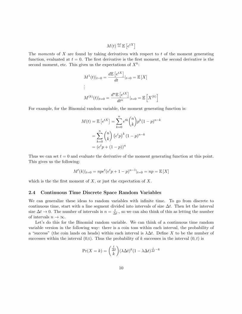
M(t)def= E
[etX]
The moments of X are found by taking derivatives with respect to t of the moment generatingfunction, evaluated at t = 0. The first derivative is the first moment, the second derivative is thesecond moment, etc. This gives us the expectations of Xk:
M1(t)|t=0 =dE[etX]
dt|t=0 = E [X]
...
M (k)(t)|t=0 =dnE
[etX]
dtn|t=0 = E
[X(k)
]For example, for the Binomial random variable, the moment generating function is:
M(t) = E[etX]
=
n∑k=0
etk(n
k
)pk(1− p)n−k
=
n∑k=0
(n
k
)(etp)k
(1− p)n−k
= (etp+ (1− p))n
Thus we can set t = 0 and evaluate the derivative of the moment generating function at this point.This gives us the following:
M ′(k)|t=0 = npet(etp+ 1− p)n−1|t=0 = np = E [X]
which is the the first moment of X, or just the expectation of X.
2.4 Continuous Time Discrete Space Random Variables
We can generalize these ideas to random variables with infinite time. To go from discrete tocontinuous time, start with a line segment divided into intervals of size ∆t. Then let the intervalsize ∆t→ 0. The number of intervals is n = t
∆t ., so we can also think of this as letting the numberof intervals n→∞.
Let’s do this for the Binomial random variable. We can think of a continuous time randomvariable version in the following way: there is a coin toss within each interval, the probability ofa “success” (the coin lands on heads) within each interval is λ∆t. Define X to be the number ofsuccesses within the interval (0,t). Thus the probability of k successes in the interval (0, t) is
Pr(X = k) =
( t∆t
k
)(λ∆t)k(1− λ∆t)
t∆t−k
10
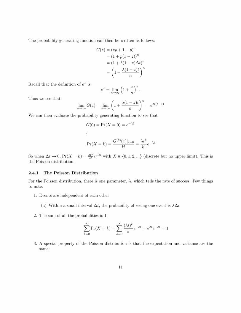
The probability generating function can then be written as follows:
G(z) = (zp+ 1− p)n
= (1 + p(1− z))n
= (1 + λ(1− z)∆t)n
=
(1 +
λ(1− z)tn
)nRecall that the definition of ex is
ex = limn→∞
(1 +
x
n
)n.
Thus we see that
limn→∞
G(z) = limn→∞
(1 +
λ(1− z)tn
)n= eλt(z−1)
We can then evaluate the probability generating function to see that
G(0) = Pr(X = 0) = e−λt
...
Pr(X = k) =G(k)(z)|z=0
k!=λtk
k!e−λt
So when ∆t→ 0, Pr(X = k) = λtk
k! e−λt with X ∈ 0, 1, 2, ... (discrete but no upper limit). This is
the Poisson distribution.
2.4.1 The Poisson Distribution
For the Poisson distribution, there is one parameter, λ, which tells the rate of success. Few thingsto note:
1. Events are independent of each other
(a) Within a small interval ∆t, the probability of seeing one event is λ∆t
2. The sum of all the probabilities is 1:
∞∑k=0
Pr(X = k) =
∞∑k=0
(λt)k
ke−λt = eλte−λt = 1
3. A special property of the Poisson distribution is that the expectation and variance are thesame:
11
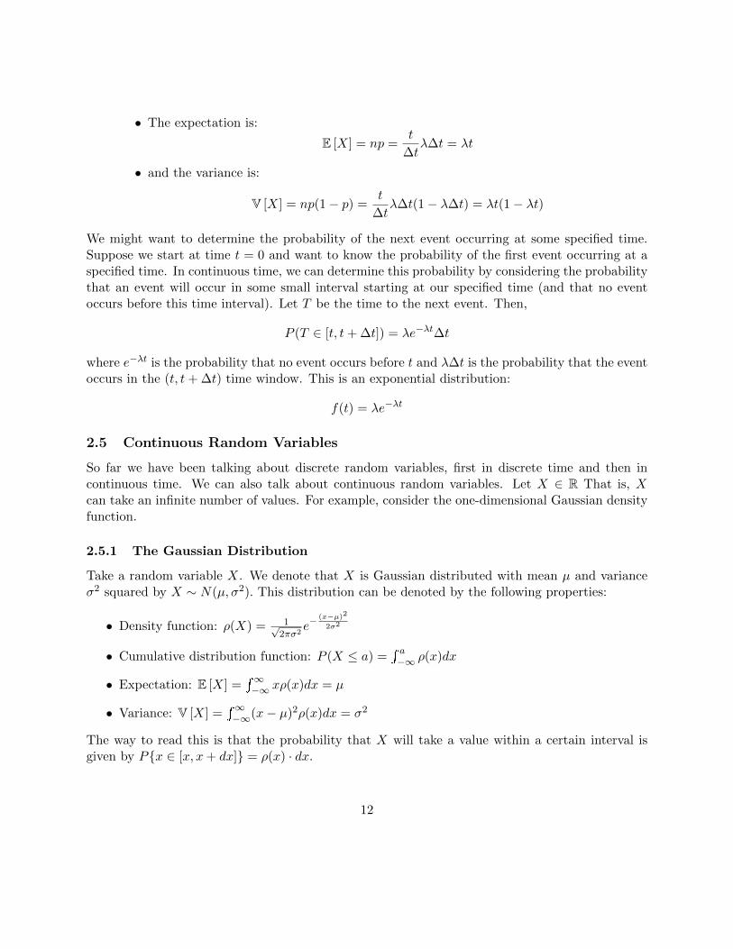
• The expectation is:
E [X] = np =t
∆tλ∆t = λt
• and the variance is:
V [X] = np(1− p) =t
∆tλ∆t(1− λ∆t) = λt(1− λt)
We might want to determine the probability of the next event occurring at some specified time.Suppose we start at time t = 0 and want to know the probability of the first event occurring at aspecified time. In continuous time, we can determine this probability by considering the probabilitythat an event will occur in some small interval starting at our specified time (and that no eventoccurs before this time interval). Let T be the time to the next event. Then,
P (T ∈ [t, t+ ∆t]) = λe−λt∆t
where e−λt is the probability that no event occurs before t and λ∆t is the probability that the eventoccurs in the (t, t+ ∆t) time window. This is an exponential distribution:
f(t) = λe−λt
2.5 Continuous Random Variables
So far we have been talking about discrete random variables, first in discrete time and then incontinuous time. We can also talk about continuous random variables. Let X ∈ R That is, Xcan take an infinite number of values. For example, consider the one-dimensional Gaussian densityfunction.
2.5.1 The Gaussian Distribution
Take a random variable X. We denote that X is Gaussian distributed with mean µ and varianceσ2 squared by X ∼ N(µ, σ2). This distribution can be denoted by the following properties:
• Density function: ρ(X) = 1√2πσ2
e−(x−µ)2
2σ2
• Cumulative distribution function: P (X ≤ a) = a−∞ ρ(x)dx
• Expectation: E [X] =∞−∞ xρ(x)dx = µ
• Variance: V [X] =∞−∞(x− µ)2ρ(x)dx = σ2
The way to read this is that the probability that X will take a value within a certain interval isgiven by Px ∈ [x, x+ dx] = ρ(x) · dx.
12
Recall that the nth moment of X is defined as
E [xp] =
∞−∞
xpρ(x)dx.
If we assume µ = 0, the pth moment function of X can be simplified as
E [xp] =
∞−∞
xpρ(x)dx
=
∞−∞
xp1√
2πσ2e−
x2
2σ2
=1√
2πσ2
∞−∞
xp−1xe−x2
2σ2 dx
To solve this, we use integration by parts. We let u = xp−1 and dv = xe−x2
2σ2 . Thus du =
(p− 1)xp−2 and v = −σ2e−x2
2σ2 . Therefore we see that
E [xp] =σ2
√2πσ2
[(xp−1e−x2
2σ2 )
∣∣∣∣∞−∞
+
∞−∞
e−x2
2σ2 (p− 1)xp−2dx].
Notice that the constant term vanishes at both limits. Thus we get that
E [xp] =σ2(p− 1)√
2πσ2
∞−∞
e−x2
2σ2 xp−2dx
= σ2(p− 1)E[xp−2
]Thus, using the base cases of the mean and the variance, we have a recursive algorithm for
finding all of the further variances. Notice that since we assumed µ = 0, we get that E [xp] = 0 forevery odd p. For every even p, we can solve the recursive equation to get
E [xp] =
(σ2
2
) p2 p!(p
2
)!
= (p− 1)!!σp
where the double factorial a!! means to multiply only the odd numbers from 1 to a.
2.5.2 Generalization: The Multivariate Gaussian Distribution
We now generalize the Gaussian distribution to multiple dimensions. Let X be a vector of n vari-ables. Thus we define X ∼ N(µ,Σ) to be a random variable following the probability distribution
ρ(x) =1√
(2π)n det Σe−
12
(x−µ)TΣ−1(x−µ)
13
where x, µ ∈ Rn and Q ∈ Rn×n. Notice that E [x] = µ and thus µ is a vector of the means whilethe variance is given by Σ:
Σ =
V ar(X1) Cov(X1, X2) . . . Cov(X1, Xn)
Cov(X1, X2). . . Cov(X2, Xn)
.... . .
...Cov(X1,Xn) Cov(X2, Xn) . . . V ar(Xn)
=
σ2X1
σX1X2 . . . σX1Xn
σX1X2
. . . σX2Xn...
. . ....
σX1Xn σX2Xn . . . σ2Xn
and thus, since Σ gives the variance in each component and the covariance between components,it is known as the Variance-Covariance Matrix.
2.5.3 Gaussian in the Correlation-Free Coordinate System
Assume µ = 0. Since Σ is positive definite and symmetric matrix, Σ has a guaranteed eigendecom-position
Σ = UΛUT
where Λ is a diagonal matrix of the eigenvalues and U is a matrix where the ith column is theith eigenvector. Thus we notice that
det(Q) = det(UΛUT ) = det(U)2 det(Λ) = λ1λ2...λn
since det(U) = 1 (each eigenvector is of norm 1). Noting that the eigenvector matrix satisfies theproperty UT = U−1 we can define a new coordinate system y = Ux and substitute to get
ρ(y) =1√
(2π)n det Σe−
12xTUTUΣ−1UUT x =
1√(2π)n det Λ
e−12yTΛy =
n∏i=1
1√(2πλi)
e− y2
i2λi
where λi is the ith eigenvalue. Notice that in the y-coordinate system, each of the components areuncorrelated. Because this is a Gaussian distribution, this implies that each component of y is aGaussian random variance yi ∼ N(0, λi).
2.6 Gaussian Distribution in PDEs
Suppose we have the diffusion equation
∂p(x, t)
∂t=
1
2
∂2p(x, t)
∂x2
p(x, 0) = ψ(x)
The solution to this problem is a Gaussian distribution
p(x, t) =1
2πte−
x2
2t
14
Heret acts like the variance, with σ2 = t. Since Green’s function for this PDE is simply the Gaussiandistribution, the general solution can be written simply as the convolution
p(x, t) =
1
2πte−
(x−y)2
2t p(y, 0)dy.
Suppose we are in n dimensional space and matrices Q = QT are both positive and finite, and thatQi,j are the entries of Q. Thus look at the PDE
∂p(x, t)
∂t=
1
2Σni,j=1qi,j
∂
∂xi
∂
∂xjp(x, t)
=1
2
(∇p(t, x)TQ∇p(x, t)
)The solution to this PDE is a multivariate Gaussian distribution
p(x, t) =1√
det(Q)(2πt)nexp(−xT (2Qt)−1x)
where the covariance matrix, Σ = tQ scales linearly with t. This shows a strong connection betweenthe heat equation (diffusion) and the Gaussian distribution, a relation we will expand upon later.
2.7 Independence
Two events are defined to be independent if the measure of doing both events is their product.Mathematically we say that two events P1 and P2 are independent if
µ(P1 ∩ P2) = µ(P1)µ(P2).
This definition can be generalized to random variables. By definition X and Y are independentrandom variables if ρ(x, y) = ρx(x)ρy(y) which is the same as saying that the joint probabilitydensity is equal to the product of the marginal probability densities
ρx(x) =
∞−∞
ρ(x, y)dy,
and ρy is defined likewise.
2.8 Conditional Probability
The probability of the event P1 given that P2 has occurred is defined as
µ(P1|P2) =µ(P1 ∩ P2)
µ(P2)
An important theorem here is Bayes’s rule. Bayes’ rule can also be referred to as “the flip-floptheorem”. Let’s say we know the probability of P1 given P2. Bayes’ theorem let’s us flip this
15
around and calculate the probability of P2 given P1 (note: these are not necessarily equal! Theprobability of having an umbrella given that it’s raining is not the same as the probability of raininggiven that you have an umbrella!). Mathematically, Bayes’ rule is the equation
µ(P2|P1) =µ(P1|P2)µ(P2)
µ(P1)
Bayes’s rule also works for the probability density functions. For the probability density functionsof random variables X and Y we get that
p(x|y) =p(y|x)p(x)
p(y).
2.9 Change of Random Variables
Suppose we know a random variable Y : P → Rn and we wish to change it via some functionφ : Rn → Rm to the random variable X as X = φ(Y ). How do we calculate ρ(x) from ρ(y)? Noticethat if we define
Range(φ) = x|x = φ(y) for some y
then ρ(x) = 0 if x /∈ Range(φ) (since y will never happen and thus x will never happen). For theother values, we note that using calculus we get
dx
dy= φ′(y)
Suppose x ∈ S. This means that we want to look for the relation such that
Pr (x ∈ (x, x+ dx)) = Pr (y ∈ (y, y + dy))
orp(x)|dx| = ρ(y)|dy|
and thus
ρ(x) = ρ(y)|dydx| = ρ(y)
|φ′(y)|
where y = φ−1(x).
2.9.1 Multivariate Changes
If there are multiple variables, then this generalizes to
ρ(x) =∑
y|φ(y)=x
ρ(y)1
∇φ(y)ρ(φ−1(y))
16
2.10 Empirical Estimation of Densities
Take a probability density ρ with a vector of parameters (θ1, . . . , θm). We write this together asρ(θ1,...,θm)(x). Suppose that given data we wish to find the “best parameter set” that matchesthe data. This would mean we would want to find the parameters such that the probability ofgenerating the data that we see is maximized. Assuming that each of n data points are fromindependent samples, the probability of getting all n data points is the probability of seeing eachindividual data point all multiplied together. Thus the likelihood of seeing a given set of n datapoints is
L(x; θ) =n∏i=1
ρ(θ1,...,θm)(xi)
where we interpret L(x; θ) as the probability of seeing the data set of the vector x given thatwe have chosen the parameters θ. Maximum likelihood estimation simply means that we wish tochoose the parameters θ such that the probability of seeing the data is maximized, and so our bestestimate for the parameter set, θ, is calculated as
θ = maxθL(x; θ).
Sometimes, it’s more useful to use the Log-Likelihood
l(x; θ) =
n∑i=1
ρ(θ1,...,θm)(xi)
since computationally this uses addition of the probabilities instead of the product (which in someways can be easier to manipulate and calculate). It can be proven that an equivalent estimator forθ is
θ = maxθl(x; θ).
3 Introduction to Stochastic Processes: Jump Processes
In this chapter we will develop the ideas of stochastic processes without “high-powered mathemat-ics” (measure theory). We develop the ideas of Markov processes in order to intuitively developthe ideas of a jump process where the probability of jumps are Poisson distributed. We then usethis theory of Poisson jump processes in order to define the Brownian motion and prove its prop-erties. Thus by the end of this chapter we will have intuitively defined the SDE and elaborated itsproperties.
3.1 Stochastic Processes
A stochastic process is the generalization of a random variable to being a changing function in time.Formally, we define a stochastic process as a collection of random variables X(t)t≥0 where X(t)is a random variable for the value of X at the time t. This can also be written equivalently as Xt.
17
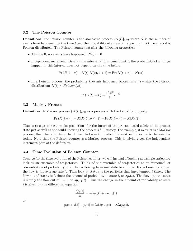
3.2 The Poisson Counter
Definition: The Poisson counter is the stochastic process N(t)t≥0 where N is the number ofevents have happened by the time t and the probability of an event happening in a time interval isPoisson distributed. The Poisson counter satisfies the following properties:
• At time 0, no events have happened: N(0) = 0
• Independent increment: Give a time interval τ form time point t, the probability of k thingshappen in this interval does not depend on the time before:
Pr (N(t+ τ)−N(t)|N(s), s < t) = Pr (N(t+ τ)−N(t))
• In a Poisson process, the probability k events happened before time t satisfies the Poissondistribution: N(t) ∼ Poisson(λt),
Pr(N(t) = k) =(λt)k
k!e−λt
3.3 Markov Process
Definition: A Markov process X(t)t≥0 as a process with the following property:
Pr (X(t+ τ) = X|X(δ), δ ≤ t)) = PrX(t+ τ) = X|X(t))
That is to say: one can make predictions for the future of the process based solely on its presentstate just as well as one could knowing the process’s full history. For example, if weather is a Markovprocess, then the only thing that I need to know to predict the weather tomorrow is the weathertoday. Note that the Poisson counter is a Markov process. This is trivial given the independentincrement part of the definition.
3.4 Time Evolution of Poisson Counter
To solve for the time evolution of the Poisson counter, we will instead of looking at a single trajectorylook at an ensemble of trajectories. Think of the ensemble of trajectories as an “amount” orconcentration of probability fluid that is flowing from one state to another. For a Poisson counter,the flow is the average rate λ. Thus look at state i is the particles that have jumped i times. Theflow out of state i is λ times the amount of probability in state i, or λpi(t). The flow into the stateis simply the flow out of i− 1, or λpi−1(t). Thus the change in the amount of probability at statei is given by the differential equation
dpi(t)
dt= −λpi(t) + λpi−1(t).
orpi(t+ ∆t)− pi(t) = λ∆tpi−1(t)− λ∆tpi(t).
18
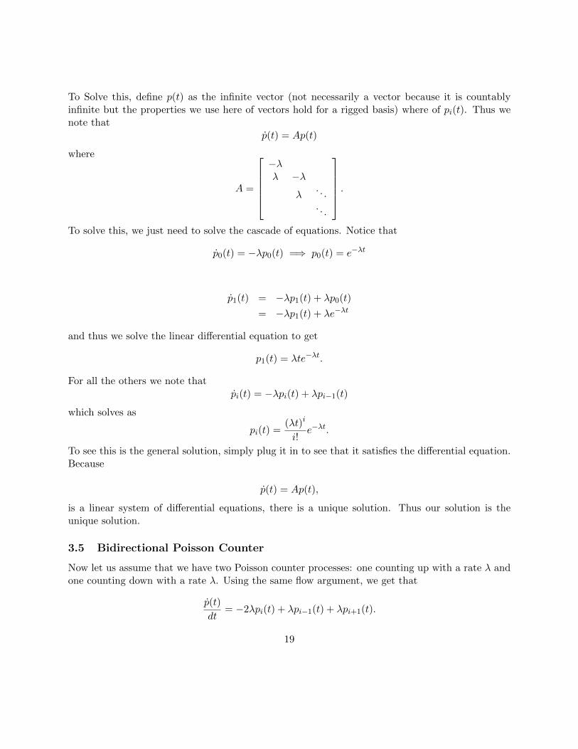
To Solve this, define p(t) as the infinite vector (not necessarily a vector because it is countablyinfinite but the properties we use here of vectors hold for a rigged basis) where of pi(t). Thus wenote that
p(t) = Ap(t)
where
A =
−λλ −λ
λ. . .. . .
.To solve this, we just need to solve the cascade of equations. Notice that
p0(t) = −λp0(t) =⇒ p0(t) = e−λt
p1(t) = −λp1(t) + λp0(t)
= −λp1(t) + λe−λt
and thus we solve the linear differential equation to get
p1(t) = λte−λt.
For all the others we note thatpi(t) = −λpi(t) + λpi−1(t)
which solves as
pi(t) =(λt)i
i!e−λt.
To see this is the general solution, simply plug it in to see that it satisfies the differential equation.Because
p(t) = Ap(t),
is a linear system of differential equations, there is a unique solution. Thus our solution is theunique solution.
3.5 Bidirectional Poisson Counter
Now let us assume that we have two Poisson counter processes: one counting up with a rate λ andone counting down with a rate λ. Using the same flow argument, we get that
p(t)
dt= −2λpi(t) + λpi−1(t) + λpi+1(t).
19
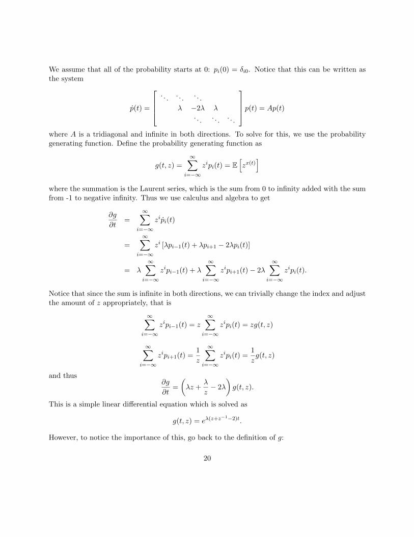
We assume that all of the probability starts at 0: pi(0) = δi0. Notice that this can be written asthe system
p(t) =
. . .
. . .. . .
λ −2λ λ. . .
. . .. . .
p(t) = Ap(t)
where A is a tridiagonal and infinite in both directions. To solve for this, we use the probabilitygenerating function. Define the probability generating function as
g(t, z) =
∞∑i=−∞
zipi(t) = E[zx(t)
]where the summation is the Laurent series, which is the sum from 0 to infinity added with the sumfrom -1 to negative infinity. Thus we use calculus and algebra to get
∂g
∂t=
∞∑i=−∞
zipi(t)
=∞∑
i=−∞zi [λpi−1(t) + λpi+1 − 2λpi(t)]
= λ∞∑
i=−∞zipi−1(t) + λ
∞∑i=−∞
zipi+1(t)− 2λ∞∑
i=−∞zipi(t).
Notice that since the sum is infinite in both directions, we can trivially change the index and adjustthe amount of z appropriately, that is
∞∑i=−∞
zipi−1(t) = z∞∑
i=−∞zipi(t) = zg(t, z)
∞∑i=−∞
zipi+1(t) =1
z
∞∑i=−∞
zipi(t) =1
zg(t, z)
and thus∂g
∂t=
(λz +
λ
z− 2λ
)g(t, z).
This is a simple linear differential equation which is solved as
g(t, z) = eλ(z+z−1−2)t.
However, to notice the importance of this, go back to the definition of g:
20
g(t, z) =∞∑
i=−∞zipi(t).
Notice that, if we look at the nth derivative, only one term, the i = n term, does not have a z. Thusif we take z = 0 (and discard all terms that blow up), we see that this singles out term which isequal to n!pi(t). This leads us to the fundamental property of the probability generating function:
pi(t) =g(k)(t, k)
k!|z=0.
Thus we can show by induction using this formula with our closed form solution of the probabilitygenerating function that
pn(t) = e−2λt∞∑m=0
(2λt)2m
22mm!(n+m)!= e−2λtIn(2λt)
where In(x) is the nth Bessel function.
3.6 Discrete-Time Discrete-Space Markov Process
Definition: a discrete-time stochastic process is a sequence of random variablesX = X1, X2, ..., Xn.Xn is the state of the process X at time n and X0 is the initial state. This process is called adiscrete-time Markov Chain if for all m and all possible states i0, i1, ...i, j ∈ X,
Pr (Xn+1 = j|Xn = in, . . . , X0 = i0) = Pr (Xn+1 = j|Xn = in) = Pij .
This definition means that the probability of transition to another state simply depends on whereyou are right now. This can be represented as a graph where your current state is the node i. Theprobability of transition from state i to state j is simply Pij , the one-step transition probability.Define
−−→P (t) = P (t) =
P1(t)...
Pn(t)
as the vector of state probabilities. The way to interpret this is as though you were running manysimulations, then the ith component of the vector is the percent of the simulations that are currentlyat state i. Since the transition probabilities only depend on the current state, we can write theiteration equation
P (t+ 1) = AP (t)
where
A =
P11 P12 · · · P1n
P21 P22 · · · P2n...
.... . .
...Pn1 Pn2 · · · Pnn
.
21
Notice that this is simply a concise way to write the idea that at every timestep, Pi,j percent ofthe simulations at state i transfer to state j. Notice then that the probabilities of transitioning atany given time will add up to 1 (the probability of not moving is simply Pi,i).
Definition: A Regular Markov Chain as a Markov Chain for which some power n of itstransition matrix A has only positive entries.
3.7 Continuous-Time Discrete-Space Markov Chain
Define a stochastic process in continuous time with discrete finite state space to be a Markov chainif
Pr (Xn+1 = j|Xn = in, ..., X0 = i0) = pij(tn+1 − tn)
where pij is the solution of the forward equation
P ′(t) = P (t)Q
where Q is a transition rate matrix which used to describe the flow of probability juices from statei to the state j. Notice that
P ′(t) = P (t)Q
P ′(t+ h)− P ′(t)h
= P ′(t)Q
P (t+ h) = (I +Qh)P (t)
P (t+ h) = AP (t)
and thus we can think of a continuous-time Markov chain as a discrete-time Markov chain withinfinitely small timesteps and a transition matrix
A = I +Qh
Note that the transition rate matrix Q satisfies the following properties:
1. Transition flow between state i and j qij > 0 when i 6= j;
2. Transition probability from i and i aij = qijh;
3.∑n
j=1 qij = 0, qii = −∑
j 6=i qij
Property 1 is stating that the transition rate matrix is composed only “rates from i” and thus theyare all positive values. Property 2 is restating the relation between Q and A. Property 3 is statingthat the diagonal of Q is composed of the flows into the state i, and thus it will be a negativenumber. One last property to note is that since
P ′(t) = P (t)Q
22
we get thatP (t) = P (0)eQt
where eQt is the matrix exponential (defined by its Taylor Series expansion being the same as thenormal exponential). This means that there exists a unique solution to the time evolution of theprobability densities. This is an interesting fact to note: even though any given trajectory evolvesrandomly, the way a large set of trajectories evolve together behaves deterministically.
3.7.1 Example: DNA Mutations
Look at a many bases of DNA. Each can take four states: A, T,C,G Denote the percent that arein state i at the time t as pi(t). We write our system as the vector
P (t) = (pA(t), pG(t), pC(t), pT (t))T
Define Q by the mutation rates from A to G, C to T, etc (yes, this is a very simplistic model. Chillbra.). We get that the evolution of the probability of being in state i at time t is given by thedifferential equation
P ′(t) = QP (t).
Since we have mathematized this process, we can now use our familiar rules to investigate thesystem. For example, if we were to run this system for a very long time, what percent of the baseswill be A? Since this is simply a differential equation, we find this by simply looking at the steadystate: the P (t) s.t. P ′(t) = 0. Notice that means that we have
0 = QP (t) = λ
since 0 is just a constant. Thus the vector P that satisfies this property is an eigenvector of Q. Thismeans that the eigenvector of Q corresponding to the eigenvalue of 0 gives the long run probabilitiesof being in state i respectively.
3.8 The Differential Poisson Counting Process and the Stochastic Integral
We can intuitively define the differential Poisson Counting Process is the process that describes thechanges of a Poisson CounterNt (or equivalently N(t)). Define the differential stochastic processdNt by its some integral
Nt =
t
0dNt.
To understand dNt, let’s investigate some of its properties. Since Nt ∼ Poisson(λt), we know that
E [Nt] = λt = E[ t
0dNt
].
23
Since E is defined as some kind of a summation or an integral, we assume that dN2t is bounded
which, at least in the normal calculus, lets us swap the ordering of integrations. Thus
λt =
t
0E [dNt] .
Since the expected value makes a constant, we intuit that
λt =
t
0αdt = αt
and thusE [dNt] = λ.
Notice this is simply saying that dNt represents the “flow of probability” that is on average λ.Using a similar argument we also note that the variance of dNt = λ. Thus we can think of theequation the term dNt as a kind of a limit, where
N(t+ dt)−N(t) = dNt
is probability of jumping k times in the increment dt which is given by the probability distribution
P (k jumps in the interval (t, t+ dt)) =(λdt)k
k!e−λdt
Then how do we make sense of the integral? Well, think about writing the integral as a Riemannsum: t
0dNt = lim
∆t→0
n−1∑i=0
(N(ti+1)−N(ti))
where ti = i∆t. One way to understand how this is done is algorithmically/computationally. Let’ssay you wanted to calculate one “stochastic trajectory” (one instantiation) of N(t). What we cando is pick a time interval dt. We can get N(t) by, at each time step dt, sample a value from theprobability distribution
P (k jumps in the interval (t, t+ dt)) =(λdt)k
k!e−λdt
and repeatedly add up the number of jumps such that N(t) is the total number of jumps at timet. This will form our basis for defining and understanding stochastic differential equations.
3.9 Generalized Poisson Counting Processes
We now wish to generalize the counting processes. Define a counting process X(t) as
dX(t) = f(X(t), t)dt+ g(X(t), t)dN(t)
24
where f is some arbitrary function describing deterministic changes in time where g defines the“jumping” properties. The way to interpret this is as a time evolution equation for X. As weincrement in time by ∆t, we add f(X(t), t) to X. If we jump in that interval, we also add g(X(t), t).The probability of jumping in the interval is given by
P (k jumps in the interval (t, t+ dt)) =(λdt)k
k!e−λdt
Another way of thinking about this is to assume that the first jump happens at a time t1. ThenX(t) evolves deterministically until t1 where it jumps by g(X(t), t), that is
limt→t+1
X(t) = g
(limt→t−1
X(t), t
)+ limt→t−1
X(t).
Notice that we calculate the jump using the left-sided limit. This is known as Ito’s calculus andit is interpreted as the jump process “not knowing” any information about the future, and thus itjumps using only previous information.
We describe the solution to the SDE once again using an integral, this time we write it as
X(t) = X(0) +
t
0f(X(t), t)dt+
t
0g(X(t), t)dN(t).
Notice that the first integral is simply a deterministic integral. The second one is a stochasticintegral. It can once again be understood as a Riemann summation, this time
t
0g(X(t), t)dNt = lim
∆t→0
n−1∑i=0
g(X(ti), ti) (N(ti+1)−N(ti)) .
We can understand the stochastic part the same as before simply as the random amount of jumpsthat happen in the interval (t, t + dt). However, now we multiply the number of jumps in theinterval by g(X(ti), ti), meaning “the jumps have changing amounts of power”.
3.10 Important Note: The Defining Feature of Ito’s Calculus
It is important to note that g is evaluated using the X and t before the jump. This is the definingprinciple of the Ito Calculus and corresponds to the “Left-Hand Rule” for Riemann sums. UnlikeNewton’s calculus, the left-handed, right-handed, and midpoint summations do not converge to thesame value in the stochastic calculus. Thus all of these different ways of summing up intervals inorder to solve the integral are completely different calculi. Notably, the summation principle whichuses the midpoints
t
0g(X(t), t)dNt = lim
∆t→0
n−1∑i=0
(g(X(ti+1), ti+1) + g(X(ti), ti)
2
)(N(ti+1)−N(ti)) .
25
is known as the Stratonovich Calculus. You may ask, why choose Ito’s calculus? In some sense, itis an arbitrary choice. However, it can be motivated theoretically by the fact that Ito’s Calculus isthe only stochastic calculus where the stochastic adder g does not “use information of the future”,that is, the jump sizes do not adjust how far they will jump given the future information of knowingwhere it will land. Thus, in some sense, Ito’s Calculus corresponds to the type of calculus we wouldbelieve matches the real-world. Ultimately, because these give different answers, which calculusbest matches the real-world is an empirical question that could be investigated itself.
3.11 Example Counting Process
Define the counting processdXt = Xtdt+XtdNt.
Suppose that the jumps occur at t1 < t2 < . . . . Thus before t1, we evolve deterministically as
dXt = Xtdt
and thus X(t) = et before t1. At t1, we take this value and jump by Xt1 . Thus since immediatelybefore the jump we have a value et1 , immediately after the jump we have et1 + et1 = 2et1 . We onceagain it begins to evolve as
dXt = Xtdt
but now with the initial condition X(t1) = 2et1 . We see that in this interval the linear equationsolves to X(t) = 2et. Now when we jump at t2, we have the value 2et2 and jump by 2et2to get 4et2
directly after the jump. Seeing the pattern, we get that
X(t) =
et, 0 ≤ t ≤ t12et, t1 ≤ t ≤ t2...
...
2net, tn ≤ t ≤ tn+1
3.12 Ito’s Rules for Poisson Jump Process
Given the SDE
dx(t) = f(x(t), t)dt+
n∑i=1
gi(x(t), t)dNi
where x ∈ R, Ni is a Poisson counter with rate λi, f : Rn → Rn, gi : Rn → Rn. Define Y = ψ(X, t)as some random variable whose values are determined as a function of X and t. How do we finddy(t), the time evolution of y? There are two parts: the determinsitic changes and the stochastic
26
jumps. The deterministic changes are found using Newton’s calculus. Notice using Newtoniancalculus that
∆Deterministic =∂ψ
∂t
∂t
∂t+∂ψ
∂x
∂x
∂t=∂ψ
∂t+∂ψ
∂x(dx)deterministic =
∂ψ
∂t+∂ψ
∂xf(x).
The second part are the stochastic changes due to jumping. Notice that if the Poisson counterprocess i jumps in the interval, the jump will change x from x to x + gi. This means that y willchange from ψ(x, t) to ψ(x+gi(x), t). Thus the change in y due to jumping is the difference betweenthe two times the number of jumps, calculated as
∆Jumps =
n∑i=1
[ψ(x+ gi(x))− ψ(x, t)]dNi,
where dNi is the number of jumps in the interval. This approximation is not correct if some processjumps multiple times in the interval, but if the interval is of size dt ([t, t+dt]), then the probabilitythat a Poisson process jumps twice goes to zero as dt→ 0. Thus this approximation is correct forinfinitesimal changes. Putting these terms together we get
dψ(x, t) = ∆Deterministic + ∆Jumps
= dy(t) = dψ(x, t) =∂ψ
∂tdt+
∂ψ
∂xf(x)dt+
m∑i=1
[ψ(x+ gi(x))− ψ(x, t)]dNi.
which is Ito’s Rule for Poisson counter processes.
3.12.1 Example Problem
Let
dx(t) = −x(t)dt+ dN1(t)− dN2(t)
where N1(t) is a Poisson counter with rate λ1 and N2(t) is a Poisson counter with rate λ2. Let ussay we wanted to know the evolution of Y = X2. Thus ψ(X, t) = X2. Using Ito’s Rules, we get
dx2(t) = 2x(−x(t))dt+ ((x+ 1)2 − x2)dN1 + ((x− 1)2 − x2)dN2
= −2x2dt+ (2x+ 1)dN1 + (1− 2x)dN2
3.13 Dealing with Expectations of Poisson Counter SDEs
Take the SDE
dx = f(x, t)dt+
m∑i=1
gi(x, t)dNi
27
where Ni is a Poisson counter with rate λi. Notice that since Ni(t) ∼ Poisson(λt), we get
E [Ni(t)] = λt.
Also notice that because Ni(t) is a Poisson process, the probability Ni(t) will jump in interval(t, t + h) is independent of X(σ) for any σ < t. This mean that, since the current change isindependent of the previous changes, E [g(x(t), t)dNi(t)] = E [g(x(t), t)]E [dNi] = λiE [g(x(t), t)].Thus we get the fact that
E [x(t+ h)− x(t)] = E [f(x, s)h] +m∑i=1
E [g(x(t), t)dNi(t)]
= E [f(x, t)]h+m∑i=1
E [gi(x, t)]λih
E [x(t+ h)− x(t)]
h= E [f(x, t)] +
m∑i=1
λiE [gi(x, t)]
and thus we take the limit as h→ 0 to get
dE [x(t)]
dt= E [f(x, t)] +
m∑i=1
λiE [gi(x, t)] .
3.13.1 Example Calculations
Given SDEdx = −xdt+ dN1 − dN2
we apply Ito’s Rule to getdE [x]
dt= −E [x] + λ1 − λ2.
Notice that this is just an ODE in E [x]. If it makes it easier to comprehend, let Y = E [x] to seethat this is simply
Y ′ = −Y + λ1 − λ2.
which we can solve using our tools from ODEs. Notice the connection here: even though thetrajectory is itself stochastic, its expectations change deterministically. Now we apply Ito’s rulesto get
dx2 = −2x2dt+ (2x+ 1)dN1 + (1− 2x)dN2
and thus we get that the expectation changes as
dE[x2]
dt= −2E
[x2]
+ (2E [x] + 1)λ1 + (1− 2E [x])λ2.
To solve this, we would first need to complete solving the ODE for E [x], then plug that solutioninto this equation to get another ODE, which we solve. However, notice that this has all beenchanged into ODEs, something we know how to solve!
28
3.13.2 Another Example Calculation
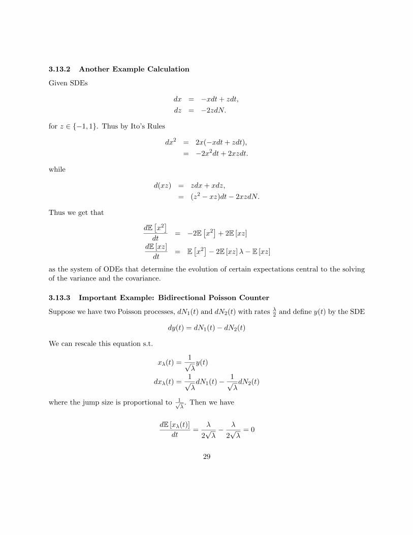
Given SDEs
dx = −xdt+ zdt,
dz = −2zdN.
for z ∈ −1, 1. Thus by Ito’s Rules
dx2 = 2x(−xdt+ zdt),
= −2x2dt+ 2xzdt.
while
d(xz) = zdx+ xdz,
= (z2 − xz)dt− 2xzdN.
Thus we get that
dE[x2]
dt= −2E
[x2]
+ 2E [xz]
dE [xz]
dt= E
[x2]− 2E [xz]λ− E [xz]
as the system of ODEs that determine the evolution of certain expectations central to the solvingof the variance and the covariance.
3.13.3 Important Example: Bidirectional Poisson Counter
Suppose we have two Poisson processes, dN1(t) and dN2(t) with rates λ2 and define y(t) by the SDE
dy(t) = dN1(t)− dN2(t)
We can rescale this equation s.t.
xλ(t) =1√λy(t)
dxλ(t) =1√λdN1(t)− 1√
λdN2(t)
where the jump size is proportional to 1√λ
. Then we have
dE [xλ(t)]
dt=
λ
2√λ− λ
2√λ
= 0
29
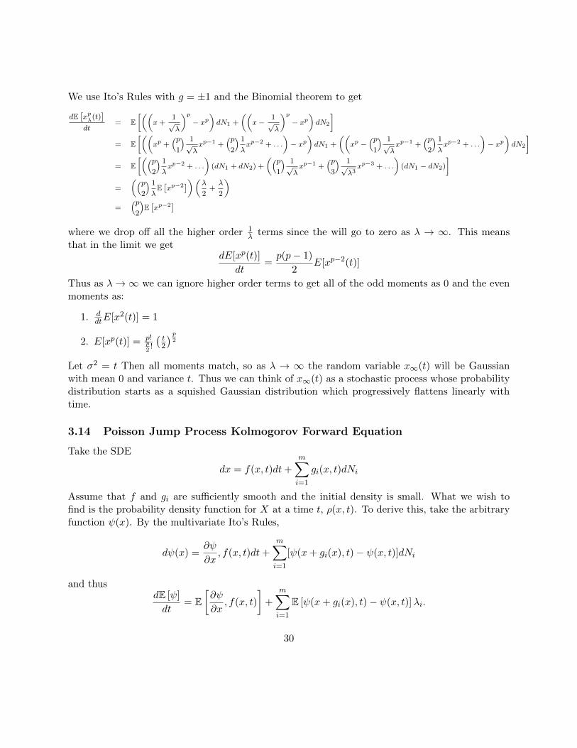
We use Ito’s Rules with g = ±1 and the Binomial theorem to get
dE[xpλ(t)
]dt
= E[((
x+1√λ
)p− xp
)dN1 +
((x−
1√λ
)p− xp
)dN2
]= E
[((xp +
(p1
) 1√λxp−1 +
(p2
) 1
λxp−2 + . . .
)− xp
)dN1 +
((xp −
(p1
) 1√λxp−1 +
(p2
) 1
λxp−2 + . . .
)− xp
)dN2
]= E
[((p2
) 1
λxp−2 + . . .
)(dN1 + dN2) +
((p1
) 1√λxp−1 +
(p3
) 1√λ3xp−3 + . . .
)(dN1 − dN2)
]=
((p2
) 1
λE[xp−2
])(λ2
+λ
2
)=
(p2
)E[xp−2
]where we drop off all the higher order 1
λ terms since the will go to zero as λ → ∞. This meansthat in the limit we get
dE[xp(t)]
dt=p(p− 1)
2E[xp−2(t)]
Thus as λ→∞ we can ignore higher order terms to get all of the odd moments as 0 and the evenmoments as:
1. ddtE[x2(t)] = 1
2. E[xp(t)] = p!p2
!
(t2
) p2
Let σ2 = t Then all moments match, so as λ → ∞ the random variable x∞(t) will be Gaussianwith mean 0 and variance t. Thus we can think of x∞(t) as a stochastic process whose probabilitydistribution starts as a squished Gaussian distribution which progressively flattens linearly withtime.
3.14 Poisson Jump Process Kolmogorov Forward Equation
Take the SDE
dx = f(x, t)dt+m∑i=1
gi(x, t)dNi
Assume that f and gi are sufficiently smooth and the initial density is small. What we wish tofind is the probability density function for X at a time t, ρ(x, t). To derive this, take the arbitraryfunction ψ(x). By the multivariate Ito’s Rules,
dψ(x) =∂ψ
∂x, f(x, t)dt+
m∑i=1
[ψ(x+ gi(x), t)− ψ(x, t)]dNi
and thusdE [ψ]
dt= E
[∂ψ
∂x, f(x, t)
]+
m∑i=1
E [ψ(x+ gi(x), t)− ψ(x, t)]λi.
30
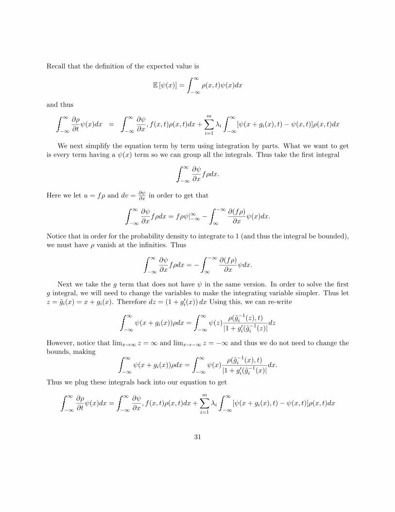
Recall that the definition of the expected value is
E [ψ(x)] =
∞−∞
ρ(x, t)ψ(x)dx
and thus
∞−∞
∂ρ
∂tψ(x)dx =
∞−∞
∂ψ
∂x, f(x, t)ρ(x, t)dx+
m∑i=1
λi
∞−∞
[ψ(x+ gi(x), t)− ψ(x, t)]ρ(x, t)dx
We next simplify the equation term by term using integration by parts. What we want to getis every term having a ψ(x) term so we can group all the integrals. Thus take the first integral
∞−∞
∂ψ
∂xfρdx.
Here we let u = fρ and dv = ∂ψ∂x in order to get that
∞−∞
∂ψ
∂xfρdx = fρψ|∞−∞ −
−∞∞
∂(fρ)
∂xψ(x)dx.
Notice that in order for the probability density to integrate to 1 (and thus the integral be bounded),we must have ρ vanish at the infinities. Thus
∞−∞
∂ψ
∂xfρdx = −
−∞∞
∂(fρ)
∂xψdx.
Next we take the g term that does not have ψ in the same version. In order to solve the firstg integral, we will need to change the variables to make the integrating variable simpler. Thus letz = gi(x) = x+ gi(x). Therefore dz = (1 + g′i(x)) dx Using this, we can re-write
∞−∞
ψ(x+ gi(x))ρdx =
∞−∞
ψ(z)ρ(g−1
i (z), t)
|1 + g′i(g−1i (z)|
dz
However, notice that limx→∞ z =∞ and limx→−∞ z = −∞ and thus we do not need to change thebounds, making ∞
−∞ψ(x+ gi(x))ρdx =
∞−∞
ψ(x)ρ(g−1
i (x), t)
|1 + g′i(g−1i (x)|
dx.
Thus we plug these integrals back into our equation to get
∞−∞
∂ρ
∂tψ(x)dx =
∞−∞
∂ψ
∂x, f(x, t)ρ(x, t)dx+
m∑i=1
λi
∞−∞
[ψ(x+ gi(x), t)− ψ(x, t)]ρ(x, t)dx
31
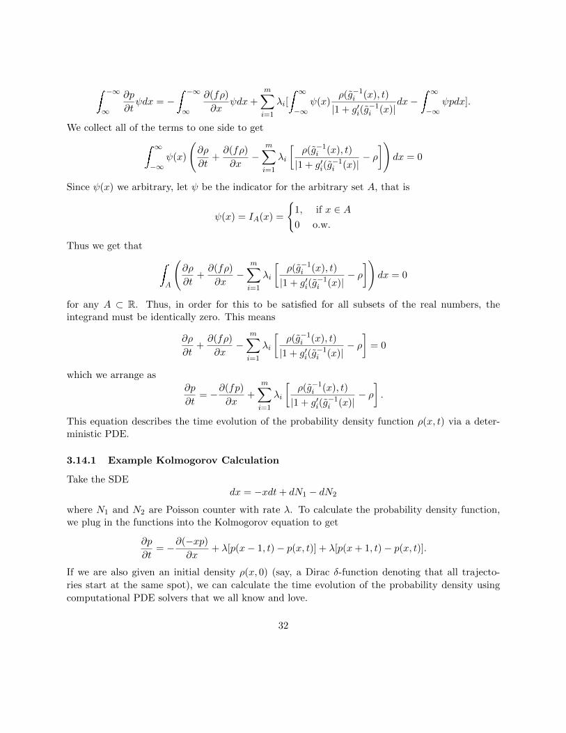
−∞∞
∂p
∂tψdx = −
−∞∞
∂(fρ)
∂xψdx+
m∑i=1
λi[
∞−∞
ψ(x)ρ(g−1
i (x), t)
|1 + g′i(g−1i (x)|
dx− ∞−∞
ψpdx].
We collect all of the terms to one side to get
∞−∞
ψ(x)
(∂ρ
∂t+∂(fρ)
∂x−
m∑i=1
λi
[ρ(g−1
i (x), t)
|1 + g′i(g−1i (x)|
− ρ])
dx = 0
Since ψ(x) we arbitrary, let ψ be the indicator for the arbitrary set A, that is
ψ(x) = IA(x) =
1, if x ∈ A0 o.w.
Thus we get that
A
(∂ρ
∂t+∂(fρ)
∂x−
m∑i=1
λi
[ρ(g−1
i (x), t)
|1 + g′i(g−1i (x)|
− ρ])
dx = 0
for any A ⊂ R. Thus, in order for this to be satisfied for all subsets of the real numbers, theintegrand must be identically zero. This means
∂ρ
∂t+∂(fρ)
∂x−
m∑i=1
λi
[ρ(g−1
i (x), t)
|1 + g′i(g−1i (x)|
− ρ]
= 0
which we arrange as
∂p
∂t= −∂(fp)
∂x+
m∑i=1
λi
[ρ(g−1
i (x), t)
|1 + g′i(g−1i (x)|
− ρ].
This equation describes the time evolution of the probability density function ρ(x, t) via a deter-ministic PDE.
3.14.1 Example Kolmogorov Calculation
Take the SDEdx = −xdt+ dN1 − dN2
where N1 and N2 are Poisson counter with rate λ. To calculate the probability density function,we plug in the functions into the Kolmogorov equation to get
∂p
∂t= −∂(−xp)
∂x+ λ[p(x− 1, t)− p(x, t)] + λ[p(x+ 1, t)− p(x, t)].
If we are also given an initial density ρ(x, 0) (say, a Dirac δ-function denoting that all trajecto-
ries start at the same spot), we can calculate the time evolution of the probability density using
computational PDE solvers that we all know and love.
32
4 Introduction to Stochastic Processes: Brownian Motion
In this chapter we will use the properties of Poisson Counting Processes in order to define Brow-nian Motion and derive a calculus for dealing with stochastic differential equations written withdifferential Wiener/Brownian terms.
4.1 Brownian Motion / The Wiener Process
Now we finally define Brownian Motion. Robert Brown is credited for first describing Brownianmotion. Brown observed pollen particles moving randomly and described the motion. Brownianmotion is also sometimes called a Wiener process because Norbert Wiener was the first person todescribe random motion mathematically. It is most commonly defined more abstractly using limitsof random walks or abstract function space definitions. We will define it using the bidirectionalPoisson counter. Recall that we define this using two Poisson processes, dN1(t) and dN2(t) withrates λ
2 and define y(t) by the SDE
dy(t) = dN1(t)− dN2(t)
We can rescale this equation s.t.
xλ(t) =1√λy(t)
dxλ(t) =1√λdN1(t)− 1√
λdN2(t).
Define the Wiener process, W (t) (or equivalently, Brownian motion B(t)) as the limit as both ofthe rates go to infinity, that is
limλ→∞
Xλ(t)→W (t).
4.2 Understanding the Wiener Process
Like before with the Poisson counter, we wish to understand what exactly dWt is. We defineW (0) = 0. Define dWt by its integral
Wt =
t
0dWt.
We can once again understand the integral by using the Riemann summation
t
0g(X, t)dWt = lim
∆t→0
n−1∑i=1
g(Xti , ti)(dWti+1 − dWti
)where ti = i∆t Notice once again that we are evaluating g using the Left-hand rule as this is thedefining feature of Ito’s Calculus: it does not use information of the future.
33
Recall that this definition is defined by the bidirectional Poisson Counter. Can we then un-derstand the interval as a number of jumps? Since since the rate of jumps is infinitely high, wecan think of this process as making infinitely many infinitely small jumps in every interval of time.Thus we cannot understand the interval as the “number of jumps” because infinitely many willoccur! However, given the proof from 3.13.3, we get that W (t) ∼ N(0, t). Thus we can think of(dWi+1 − dWi) ∼ N(0, dt), that is, the size of the increment is normally distributed. Algorithmi-cally solving the integral by taking a normally distributed random number with variance dt andmultiplying it by g to get the value of g(X, t)dWt over the next interval of time. Using Ito’s Rulesfor Wiener Processes (which we will derive shortly) we can easily prove that
1. E[(W (t)−W (s))2
]= t− s for t > s.
2. E[W (t1)W (t2)] = min(t1, t2).
Notice that this means E[(W (t+ ∆t)−W (t))2] = ∆t and thus in the limit as ∆t → 0, thenE[(W (t+ ∆t)−W (t))2]→ 0 and thus the Wiener process is continuous almost surely (with prob-ability 1). However, it can be proven that it is not differentiable with probability 1! Thus dWt issome kind of abuse of notation because the derivative of Wt does not really exist. However, we canstill use it to understand the solution to an arbitrary SDE
dXt = f(X, t)dt+ g(X, t)dWi
as the integral
Xt = X0 +
t
0f(Xt, t)dt+
t
0g(Xt, t)dWt.
4.3 Ito’s Rules for Wiener Processes
By the definition of the Wiener process, we can write
dWi =1√λ
(dNi − dN−i)
in the limit where λ→∞. We can define the stochastic differential equation (SDE) in terms of theWiener process
dXt = f(X, t)dt+
n∑i=1
gi(x)dWi = f(X, t)dt+
n∑i=1
gi(x)√λ
(dNi − dN−i)
We now define Yt = ψ(x, t). Using Ito’s Rules for Poisson Jump Processes, we get that
dYt = dψ(x, t) =∂ψ
∂tdt+
∂ψ(x, t)
∂xf(x, t)dt+
n∑i=1
(ψ
(x+
gi(x)√λ
)− ψ(x, t)
)dNi +
n∑i=1
(ψ
(x−
gi(x)√λ
)− ψ(x, t)
)dN−i.
34
To simplify this, we expand ψ by λ to get
ψ
(x+
gi(x)√λ
)= ψ(x) + ψ′(x)
gi(x)√λ
+ ψ′′(x)g2i (x)
λ+O(λ−
32 )
ψ
(x− gi(x)√
λ
)= ψ(x)− ψ′(x)
gi(x)√λ
+ ψ′′(x)g2i (x)
λ+O(λ−
32 )
to simplify to (dropping off higher-order terms)
dψ(x) =∂ψ
∂tdt+
∂ψ(x, t)
∂xf(x, t)dt+
n∑i=1
(ψ′(x)
gi(x)√λ
+ ψ′′(x)g2i (x)
λ
)dNi +
n∑i=1
(−ψ′(x)
gi(x)√λ
+ ψ′′(x)g2i (x)
λ
)dN−i,
and thus
dψ(x) =∂ψ
∂tdt+
∂ψ(x, t)
∂xf(x, t)dt+
n∑i=1
ψ′(x)gi(x)√λ
(dNi − dN−i)n∑i=1
ψ′′(x)g2i (x)
(1
λ(dNi + dN−i)
).
Let us take a second to justify dropping off the higher order terms. Recall that the Wienerprocess looks at the limit as λ→∞. In the expansion, the terms dropped off are O(λ−
32 ). Recall
that
E [dNi] =λ
2.
Thus we see that the expected contribution of these higher order terms is
limλ→∞
E[O(λ−
12 )dNi
]= 0.
However, we next note that
V [dNi] = E [dNi] =λ
2.
Thus we get that
limλ→∞
V[O(λ−
12 )dNi
]= 0.
Therefore, since the variance goes to zero, the contribution of these terms are not stochastic. Thusthe higher order terms deterministically make zero contribution (in more rigorous terms, they makeno contribution to the change with probability 1). Therefore, although this at first glace lookedlike an approximation, we were actually justified in only taking the first two terms of the Taylorseries expansion.
Sub-Calculation
To simplify this further, we need to do a small calculation. Define
dzi =1
λ(dNi + dN−i) .
35
Notice thatdE [zi]
dt=
1
λ
(λ
2+λ
2
)= 1
which meansE [zi] = t.
Using Ito’s rules
dz2i =
((zi +
1
λ
)2
− z2i
)(dNi + dN−i)
=
(2ziλ
+1
λ2
)(dNi + dN−i)
and thus
dE[z2i
]dt
=
(2E [zi]
λ+
1
λ2
)(λ
2+λ
2
)=
(2t
λ+
1
λ2
)λ
= 2t+1
λ
to make
E[z2i
]= t2 +
t
λ.
This means that
V [zi] = E[z2i
]− E [zi]
2 = t2 +t
λ− t2 =
t
λ.
Thus look atZ = lim
λ→∞zi.
This means thatE [Z] = t,
andV [Z] = 0.
Notice that since the variance goes to 0, in the limit as λ → ∞, Z is a deterministic process thatis equal to t, and thus dZ = dt.
36
Solution for Ito’s Rules
Return to
dψ(x) = ψ′(x)(f(X, t)dt+
n∑i=1
ψ′(x)gi(x)√λ
(dNi − dN−i)+n∑i=1
ψ′′(x)g2i (x)
(−ψ′(x)gi(x)√
λ+ ψ′′(x)
g2i (x)
λ
)(1
λ(dNi + dN−i)
).
Notice that the last term is simply zi. Thus we take the limit as λ→∞ to get that
dψ(x) = ψ′(x)(f(X, t)dt+
n∑i=1
ψ′(x)gi(x)dWt +
n∑i=1
ψ′′(x)g2i (x)dt
which is Ito’s Rules for an SDE. If x is a vector then we would arrive at
dφ(x) = 〈ψ(x), f(x)〉dt+n∑i=1
〈∇ψ(x), gi(x)〉dWi +1
2
n∑i=1
gi(x)T∇2ψ(x)gi(x)dt
where 〈x, y〉 is the dot product between x and y and ∇2 is the Hessian.
4.4 A Heuristic Way of Looking at Ito’s Rules
Take the SDE
dXt = f(X, t)dt+n∑i=1
gi(X, t)dWi.
DefineYt = ψ(Xt, t).
By the normal rules of calculus, we get
dψ(Xt, t) =∂ψ
∂tdt+
∂ψ
∂Xt(dXt) +
1
2
∂2ψ
∂X2t
(dXt)2
=∂ψ
∂tdt+
∂ψ
∂Xt
(f(X, t)dt+
n∑i=1
gi(X, t)dWi
)+
1
2
∂2ψ
∂X2t
(f(X, t)dt+
n∑i=1
gi(X, t)dWi
)2
=∂ψ
∂tdt+
∂ψ
∂Xt
(f(X, t)dt+
n∑i=1
gi(X, t)dWi
)+
1
2
∂2ψ
∂X2t
(f2(X, t)dt2 + f(X, t)
n∑i=1
gi(X, t)dWidt+
n∑i=1
g2i (X, t)dW 2
i
).
If we letdt× dt = 0
dWi × dt = 0
dWi × dWj =
dt : i = j0 : i 6= j
then this simplifies to
dψ(x, t) =
(∂ψ
∂t+ f(x, t)
∂ψ
∂x+
1
2
n∑i=1
g2i (x, t)
∂2ψ
∂x2
)dt+
∂ψ
∂x
n∑i=1
gi(x, t)dWi
37
which is once again Ito’s Rules. Thus we can think of Ito’s Rules is saying that dt2 is sufficientlysmall, dt and dWi are uncorrelated, and dW 2
i = dt which means that the differential Wiener processsquared is a deterministic process. In fact, we can formalize this idea as the defining property ofBrownian motion. This is captured in Levy Theorem which will be stated in 6.7.
4.5 Wiener Process Calculus Summarized
Take the SDE
dx = f(x, t)dt+n∑i=1
gi(x, t)dWi
where Wi(t) is a standard Brownian motion. We have showed that Ito’s Rules could be interpretedas:
dt× dt = 0
dWi × dt = 0
dWi × dWj =
dt : i = j0 : i 6= j
and thus if y = ψ(x, t), Ito’s rules can be written as
dy =∂ψ
∂tdt+
∂ψ
∂xdx+
1
2
∂2ψ
∂x2(dx)2
where, if we plug in dx, we get
dy = dψ(x, t) =
(∂ψ
∂t+ f(x, t)
∂ψ
∂x+
1
2
n∑i=1
g2i (x, t)
∂2ψ
∂x2
)dt+
∂ψ
∂x
n∑i=1
gi(x, t)dWi
The solution is given by the integral form:
x(t) = x(0) +
t
0f(x(s))ds+
t
0
m∑i=1
gi(x(s))dWi.
Note that we can also generalize Ito’s lemma to the multidimensional X ∈ Rn case:
dψ(X) =
⟨∂ψ
∂X, f(X)
⟩dt+
m∑i=1
⟨∂ψ
∂X, gi(X)
⟩dWi +
1
2
m∑i=1
gi(X)T∇2ψ(X)gi(X)dt
There are many other facts that we will state but not prove. These are proven using Ito’s Rules.They are as follows:
38
1. Product Rule: d(XtYt) = XtdY + YtdX + dXdY .
2. Integration By Parts: t
0 XtdYt = XtYt −X0Y0 − t
0 YtdXt − t
0 dXtdYt.
3. E[(W (t)−W (s))2
]= t− s for t > s.
4. E[W (t1)W (t2)] = min(t1, t2).
5. Independent Increments: E [(Wti −Ws1) (Wt2 −Ws2)] = 0 if [t1, s1] does not overlap [t2, s2].
6. E[ t
0 h(t)dWt
]= E [h(t)dWt] = 0.
7. Ito Isometry: E[( T
0 XtdWt
)]= E
[ T0 X2
t dt]
4.5.1 Example Problem: Geometric Brownian Motion
Look at the example stochastic process
dx = αxdt+ σxdW.
To solve this, we start with our intuition from Newton’s Calculus that this may be an exponentialgrowth process. Thus we check Ito’s equation on the logarithm ψ(x, t) = ln(x) for this process is,
d (lnx) =
(0 + (αx)
(1
x
)− 1
2
(σ2x2
)( 1
x2
))dt+
(1
x
)(σx) dW
d (lnx) =
(α− 1
2σ2
)dt+ σdW.
Thus by taking the integral of both sides we get
ln(x) =
(α− 1
2σ2
)t+ σW (t)
and then expnentiating both sides
x(t) = e(α−12σ2)t+σW (t).
Notice that since the Wiener process W (t) ∼ N(0, t), the log of x is distributed normally asN((α− 1
2σ2)t, σ2t). Thus x(t) is distributed as what is known as the log-normal distribution.
39
4.6 Kolmogorov Forward Equation Derivation
The Kolmogorov Forward Equation, also known to Physicists as the Fokker-Planck Equation, isimportant because it describes the time evolution of the probability density function. Whereas thestochastic differential equation describes how one trajectory of the stochastic processes evolves, theKolmogorov Forward Equation describes how, if you were to be running many different simulationsof the trajectory, the percent of trajectories that are around a given value evolves with time.
We will derive this for the arbitrary drift process:
dx = f(x)dt+
m∑i=1
gi(x)dWi.
Let ψ(x) be an arbitrary time-independent transformation of x. Applying Ito’s lemma for anarbitrary function we get
dψ(x, t) =
(f(x, t)
∂ψ
∂x+
1
2
n∑i=1
g2i (x, t)
∂2ψ
∂x2
)dt+
∂ψ
∂x
n∑i=1
gi(x, t)dWi
Take the expectation of both sides. Because expectation is a linear operator, we can move it insidethe derivative operator to get
d
dtE [ψ(x)] = E
[∂ψ
∂xf(x)
]+
1
2E
[m∑i=1
∂2ψ
∂x2g2i (x)
].
Notice that E [dWi] = 0 and thus the differential Wiener terms dropped out.Recall the definition of expected value is
E[ψ(x)] =
∞−∞
ρ(x, t)ψ(x)dx
where ρ(x, t) is the probability density of equaling x at a time t. Thus we get that the first term as
d
dtE [ψ(x)] =
∞−∞
∂ρ
∂tψ(x)dx
For the others, notice
E[∂ψ
∂xf(x)
]=
∞−∞
ρ(x, t)∂ψ
∂xf(x)dx.
We rearrange terms doing integration by parts. Let u = ρf and dv = ∂ψ∂x . Thus du = ∂(ρf)
∂x andv = ψ. Therefore we get that
E[∂ψ
∂xf(x)
]= [ρfψ]∞−∞ −
∞−∞
∂(ρf)
∂xψ(x)dx.
40
In order for the probability distribution to be bounded (which it must be: it must integrate to 1),
ρ must vanish at both infinities. Thus, assuming bounded expectation, E[∂ψ∂x f(x)
]< ∞, we get
that
E[∂ψ
∂xf(x)
]= −
∞−∞
∂(ρf)
∂xψ(x)dx.
The next term we manipulate similarly,
E[∂ψ2
∂x2g2i (x)
]=
∞−∞
∂2ψ
∂x2g2i (x)ρ(x, t)dx
=
[ρg2∂ψ
∂x
]∞−∞− ∞−∞
∂(g2i (x)ρ(x, t)
)∂x
∂ψ
∂xdx
=
[ρg2∂ψ
∂x
]∞−∞−
[∂(ρg2)
∂xψ
]∞−∞
+1
2
∞−∞
∂2(g2i (x)ρ(x, t)
)∂x2
ψ(x)dx
= 12
∞−∞
∂2(g2i (x)ρ(x, t)
)∂x2
ψ(x)dx
where we note that, at the edges, the derivative of ρ converges to zero since ρ converges to 0 andthus the constant terms vanish. Thus we get that
∞−∞
∂ρ
∂tψ(x)dx = −
∞−∞
∂(ρf)
∂xψ(x)dx+
1
2
∑i
∞−∞
∂(g2i ρ)
∂xψ(x)dx
which we can re-write as
∞−∞
(∂ρ
∂t+∂(ρf)
∂x− 1
2
∑i
∂(g2i ρ)
∂x
)ψ(x)dx = 0.
Since ψ(x) is arbitrary, let ψ(x) = IA(x), the indicator function for the set A:
IA(x) =
1, x ∈ A0 o.w.
Thus we get that A
(∂ρ
∂t+∂(ρf)
∂x− 1
2
∑i
∂(g2i ρ)
∂x
)dx = 0
for any arbitrary A ⊆ R. Notice that this implies that the integrand must be identically zero. Thus
∂ρ
∂t+∂(ρf)
∂x− 1
2
∑i
∂(g2i ρ)
∂x= 0,
41
which we re-arrange as
∂ρ(x, t)
∂t= − ∂
∂x[f(x)ρ(x, t)] +
1
2
m∑i=1
∂2
∂x2
[g2i (x)ρ(x, t)
],
which is the Forward Kolmogorov or the Fokker-Planck equation.
4.6.1 Example Application: Ornstein–Uhlenbeck Process
Consider the stochastic process
dx = −xdt+ dWt,
where Wt is Brownian motion. The Forward Kolmogorov Equation for this SDE is thus
∂ρ
∂t=
∂
∂x(xρ) +
1
2
∂2
∂x2ρ(x, t)
Assume that the initial conditions follow the distribution u to give
ρ(x, 0) = u(x)
and the boundary conditions are absorbing at infinity. To solve this PDE, let y = xet and applyIto’s lemma
dy = xetdt+ etdx = etdW
and notice this follows has the Forward Kolmogorov Equation
∂ρ
∂t=e2t
2
∂2ρ
∂y2.
which is a simple form of the Heat Equation. If ρ(x, 0) = δ(x), the Dirac-δ function, then we know
this solves as a Gaussian with diffusion constant e2t
2 to give us
ρ(y, t) =1√
2πe2tte−
y2
2e2tt .
and thus y ∼ N(0, e2tt). To get the probability density function in terms of x, we would simply dothe pdf transformation as described in 2.9.
4.7 Stochastic Stability
The idea of stochastic stability is that linear stability analysis for deterministic systems generalizesto stochastic systems. To see this, look at the equation
dx = axdt+ dWt.
42
Notice thatdE [x]
dt= aE [x]
and thusE [x] = E [x0] eat
which converges iff a < 0. Also notice that
dx2 = 2xdx+ dt
= 2x(axdt+ dWt) + dt
= (2ax2 + 1)dt+ dWt
and thusdE[x2]
dt= 2aE
[x2]
+ 1
which gives
E[x2]
=
(E[x2
0
]+
1
2a
)e2at
which converges iff a < 0. This isn’t a full proof, but it motivates the idea that if the deterministiccoefficient is less than 0, then, just as in the deterministic case, the system converges and is thusstable.
4.8 Fluctuation-Dissipation Theorem
Take the SDE
dX = f(X, t)dt+ g(X, t)dWt.
If there exists a stable steady state, linearize the system around a steady state
dX = Jf (Xss, t)dt+ g(Xss, t)dWt,
where Jf is the Jacobian of f defined as
Jf =
∂f1
∂x1
∂f1
∂x2. . . ∂f1
∂xn...
...∂fm∂x1
∂fm∂x2
. . . ∂fm∂xn
where ∂fi
∂xjis the partial derivative of the ith component of f by the jth component of x. The
Fluctuation-Dissipation Theorem tells us that the variance-covariance matrix of the variables,
Σ =
V ar(X1) Cov(X1, X2) . . . Cov(X1, Xn)
Cov(X1, X2). . . Cov(X2, Xn)
.... . .
...Cov(X1,Xn) Cov(X2, Xn) . . . V ar(Xn)
=
σ2X1
σX1X2 . . . σX1Xn
σX1X2
. . . σX2Xn...
. . ....
σX1Xn σX2Xn . . . σ2Xn
43
can be found at the steady state using the formula
Jf (Xss, t)Σ(Xss, t) + Σ(Xss, t)JTf (Xss, t) = −g2(Xss, t).
5 Computational Simulation of SDEs
In this chapter we outline basic procedures for the computational simulation of SDEs. For a goodintroduction to computational simulation of SDEs, refer to Higham’s An Algorithmic Introductionto Numerical Simulation of Stochastic Differential Equations. For a more complete reference onhigher-order methods, see Kloeden’s Numerical Solution of SDE Through Computer Experimentsand Iacus’s Simulation and Inference for Stochastic Differential Equations.
5.1 The Stochastic Euler Method - Euler-Maruyama Method
An intuitive way to start the computational simulation of SDEs is to look at a straight-forwardgeneralization of Euler’s method for ODEs to SDEs. First, let us recap Euler’s method for ODEs.Take the ODE
x′(t) = f(x, t).
Writing this out we getdx
dt= f(x, t)
which we can represent asdx = f(x, t)dt.
Euler’s method is to approximate the solution using “discrete-sized dt’s”. Thus we take somefixed small constant ∆t. We say that
x(t+ ∆t)− x(t) = f(x, t)∆t,
and thusx(t+ ∆t) = x(t) + f(x, t)∆t
defines a recursive solution for the value of x at a time t given values of x at previous times. Allthat is left for the approximation is some initial condition needs to be started, such as x(0) = yand thus problem is solved iteratively.
Now we take the stochastic differential equation
dX = f(X, t)dt+ g(X, t)dWt.
Once again, we define some small fixed constant ∆t and write
X(t+ ∆t)−X(t) = f(X, t)∆t+ g(X, t)∆Wt,
X(t+ ∆t) = X(t) + f(X, t)∆t+ g(X, t)∆Wt.
44
Recall from 4.2 that an interval ∆t of the Wiener process is distributed as
∆Wt = (dWt+∆t − dWt) ∼ N(0, dt).
Thus let ηi be a standard normal random variable: ηi ∼ N(0, 1). Notice that ∆Wt = ηi√dt. Thus
we can writeX(t+ ∆t) = X(t) + f(X, t)∆t+
√∆tg(X, t)ηi.
The way to interpret this is that, for each interval i, we sample a standard normal random variableηi, and iterate one step using this equation, then sample another standard normal random variableand iterate again! So this shows the strong connection between Gaussian processes and the Wienerprocess. This method for iteratively solving a stochastic differential equation is known as theEuler-Maruyama Method.
5.2 A Quick Look at Accuracy
Recall that for Euler’s method, when using a time discretization of size ∆t, we have the the accuracyof the solution is O(∆t), that is, each step approximates the change in x well, give or take an amount∆t. This is justified using Taylor series expansions, since
x(t+ ∆t) = x(t) + x′(t)∆t+O(∆t2)
and thus, if x is the real solution and X is the approximation,
x(t+ ∆t)− x(t) = x′(t)∆t+O(∆t2),
X(t+ ∆t)−X(t) = X ′(t)∆t.
We can then write that|x(t)−X(t)| ≤ C∆t
and therefore we are confident that our approximation X converges to the real solution x linearlyby ∆t (we are not confident in our answer for variations as small as ∆t2 because we dropped thoseterms off!).
We may think that this simply generalizes. However, it gets more complicated quite quickly.First of all, how do we define the difference? There are two ways to define the difference. One wayis known as the Strong Convergence. The strong convergence is the expected difference between“the real solution” and the approximation solution, that is if x is the real solution and X is ourapproximation, then the strong convergence is the factor γ defining
E [|x−X|] ≤ C∆tγ .
We can think of a different type of convergence, known as the weak convergence, as
|E [x]− E [X] | ≤ C∆tβ.
45
Notice how different these ideas of convergence are. Weak convergence means that the averagetrajectory we computationally simulate does ∆tβ good, where as strong convergence means thatevery trajectory does ∆tγ good. Thus if we are looking at properties defined by ensembles oftrajectories, then weak convergence is what we are looking at. However, if we want to know howgood a single trajectory is, we have to look at the strong convergence.
Here comes the kicker. For the Euler-Maruyama method, it has a strong convergence of order12 and a weak convergence of order 1. That’s to say it has a slower convergence than the Eulermethod, and the average properties only converge as fast as the Euler method! Thus, in practice,this method is not very practical given its extremely slow convergence.
5.3 Milstein’s Method
To understand how to make the algorithms better, we have to understand what went wrong.Why was the convergence of the stochastic method slower than that of the deterministic method?The answer comes from the Taylor series expansion. Notice that in the stochastic Taylor series(expansion using Ito’s Rules), the second order terms matter for the first-order effects because(dWt)
2 = dt! Thus, accounting for the second order Taylor series term instead write ∂g∂x = gx to
get the method
X(t+ ∆t) = X(t) +
(f(X, t)− 1
2g(X, t)gx(X, t)
)∆t+
√∆tg(X, t)ηi +
∆t
2g(X, t)gx(X, t)η2
i .
Notice that we have added a−12g(X, t)gx(X, t)dt term in order to cancel out the 1
2g(X, t)gx(X, t) (dWt)2
term in the stochastic Taylor series expansion. Notice too that we only sample one random number,but the second order term uses that random number squared. This method is known as Milstein’smethod. As you may have guessed, since it now accounts for all order 1 effects, it has order 1 strongand weak convergence.
5.4 KPS Method
As Milstein’s method is still only as good as the deterministic Euler method, I wish to give one lastmethod for the purpose of simulating SDEs for applications. For most applications, you want youconvergence order greater than 1. The simplest of such methods is the KPS method which as astrong order of convergence of 1.5 and a weak order of convergence 2. The method can be writtenas follows:
46
X(t+ ∆t) = X(t) + f∆t+ g∆Wt +∆t
2ggx
((∆Wt)
2 −∆t)
+ gfx∆Ut +1
2
(ffx +
1
2g2fxx
)∆t2
+
(fgx +
1
2g2gxx
)(∆Wt∆t−∆Ut)
+1
2g (ggx)x
(1
3(∆Wt)
2 −∆t
)∆Wt
where∆Wt =
√∆tηi
and
∆Ut =
t+∆t
t
s
tdWsds
can be written as
∆Ut =1
3∆t3λi
where λi ∼ N(0, 1), a standard normal random variable (that is not ηi!).
5.5 Simulation Via Probability Density Functions
Another method for simulating SDEs is to use the Forward Kolmogorov Equation. Recall that theSDE
dX = f(X, t)dt+ g(X, t)dWt
has a probability distribution function ρ which satisfies the PDE
∂ρ(x, t)
∂t= − ∂
∂x[f(x)ρ(x, t)] +
1
2
m∑i=1
∂2
∂x2
[g2i (x)ρ(x, t)
].
This can thus be a way to solve for the probability density using computational PDE solvers. If wehave an initial condition, X(0) = x0, then this corresponds to the initial condition ρ(x, 0) = δ(x−x0)where δ is the Dirac-δ function. This can be particularly useful for first-passage time problems,where we can set the boundary conditions as absorbing: ρ(a, t) = ρ(b, t) = 0, and thus ρ is thetotal probability distribution of trajectories that have not been absorbed. Likewise, if we wanta boundary condition where we say “trajectories reflect off the point a”, then we simply use acondition ∂ρ
∂x |x=a = 0.However, though this method may be enticing to those who are experienced with computational
PDE solvers, this method is not the holy grail because it cannot simulate trajectories. If you needthe trajectory of a single instantiation of the process, for example, “what does the stock price overtime look like?”, you cannot use this method.
47
6 Measure-Theoretic Probability for SDE Applications
Here we will get down and dirty with some measure-theoretic probability in order to define condi-tional expectations, martingales, and get further into stochastic calculus.
6.1 Probability Spaces and σ-algebras
The idea is that the probability space is simply a set of all of the events, a collection of subsetsof events (where if two events are in a subset, it is the event that both happen), and a measurewhich is a function that gives the number of how probable a collection of subsets are. These arethus define in set-theoretic terms so that they correspond to the normal rules of calculus that youwould expect.
Definition: Let Ω be a nonempty set, and let F be a collection of subsets of Ω. We say F isa σ-algebra if
1. ∅ ∈ F ,
2. A ∈ F ⇒ AC ∈ F ,
3. A1, A2, . . . ∈ F ⇒⋃∞n=1An ∈ F .
Propositions:
1. Ω ∈ F .
2. A1, A2, . . . ∈ F ⇒⋂∞n=1An ∈ F .
To prove proposition 1, notice that since ∅ ∈ F , by property 2 the compliment of the empty set,Ω, must be in F . Proposition two follows by DeMorgan’s Law. By property 3 the union is in F ,and so the union of the compliments are in F by applying property 2 to each component. Thusthe compliment of the union of the complements is in F by property 2. By DeMorgan’s Law,the intersection of the complement of the complements, or simply the intersection, must be in Fproving the proposition.
Definition: Given Ω and F , a probability measure P is a function F → [0, 1] such that:
1. P (Ω) = 1
2. A1, A2, , . . . is a sequence of disjoint subsets in F ⇒ P (⋃∞n=1An) =
∑∞i=1 P (An) (Countable
additivity)
Definition: (Ω,F , P ) is a probability space.Proposition: A1 ⊂ A2 . . . ,⊂ Ai, . . . ∈ F , then P (
⋃∞n=1An) = limn→∞ P (An) and P (
⋂∞n=1An) =
limn→∞ P (An) .These propositions come directly from the properties of measures. See a measure theory text
for more information if you do not know and you’re Curious George. There are many possibilitiesfor what kind of sample space, Ω, we may want to consider:
48
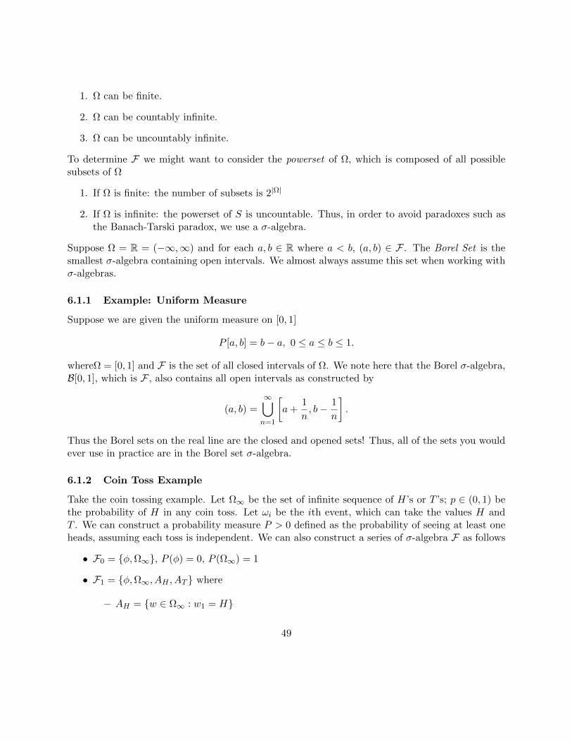
1. Ω can be finite.
2. Ω can be countably infinite.
3. Ω can be uncountably infinite.
To determine F we might want to consider the powerset of Ω, which is composed of all possiblesubsets of Ω
1. If Ω is finite: the number of subsets is 2|Ω|
2. If Ω is infinite: the powerset of S is uncountable. Thus, in order to avoid paradoxes such asthe Banach-Tarski paradox, we use a σ-algebra.
Suppose Ω = R = (−∞,∞) and for each a, b ∈ R where a < b, (a, b) ∈ F . The Borel Set is thesmallest σ-algebra containing open intervals. We almost always assume this set when working withσ-algebras.
6.1.1 Example: Uniform Measure
Suppose we are given the uniform measure on [0, 1]
P [a, b] = b− a, 0 ≤ a ≤ b ≤ 1.
whereΩ = [0, 1] and F is the set of all closed intervals of Ω. We note here that the Borel σ-algebra,B[0, 1], which is F , also contains all open intervals as constructed by
(a, b) =
∞⋃n=1
[a+
1
n, b− 1
n
].
Thus the Borel sets on the real line are the closed and opened sets! Thus, all of the sets you wouldever use in practice are in the Borel set σ-algebra.
6.1.2 Coin Toss Example
Take the coin tossing example. Let Ω∞ be the set of infinite sequence of H’s or T ’s; p ∈ (0, 1) bethe probability of H in any coin toss. Let ωi be the ith event, which can take the values H andT . We can construct a probability measure P > 0 defined as the probability of seeing at least oneheads, assuming each toss is independent. We can also construct a series of σ-algebra F as follows
• F0 = φ,Ω∞, P (φ) = 0, P (Ω∞) = 1
• F1 = φ,Ω∞, AH , AT where
– AH = w ∈ Ω∞ : w1 = H
49
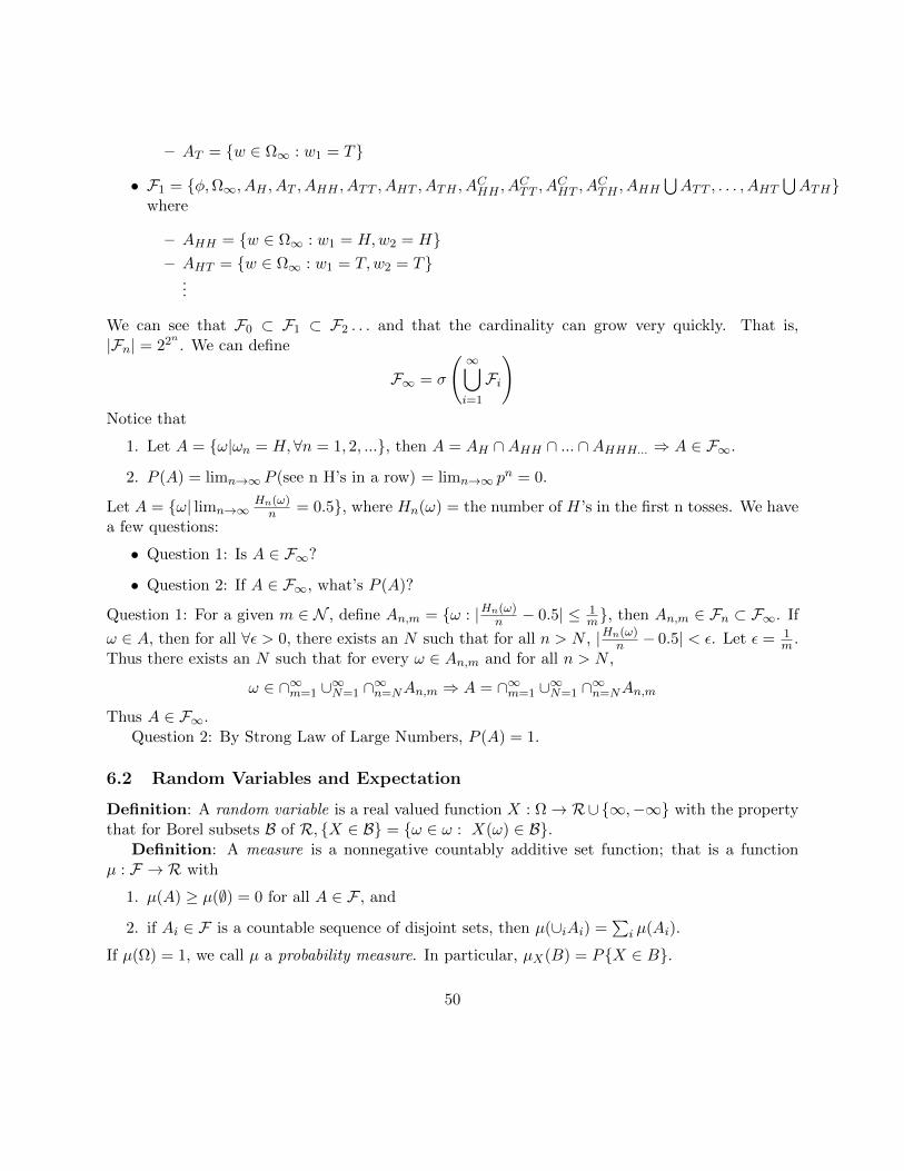
– AT = w ∈ Ω∞ : w1 = T
• F1 = φ,Ω∞, AH , AT , AHH , ATT , AHT , ATH , ACHH , ACTT , ACHT , ACTH , AHH⋃ATT , . . . , AHT
⋃ATH
where
– AHH = w ∈ Ω∞ : w1 = H,w2 = H– AHT = w ∈ Ω∞ : w1 = T,w2 = T
...
We can see that F0 ⊂ F1 ⊂ F2 . . . and that the cardinality can grow very quickly. That is,|Fn| = 22n . We can define
F∞ = σ
( ∞⋃i=1
Fi
)Notice that
1. Let A = ω|ωn = H,∀n = 1, 2, ..., then A = AH ∩AHH ∩ ... ∩AHHH... ⇒ A ∈ F∞.
2. P (A) = limn→∞ P (see n H’s in a row) = limn→∞ pn = 0.
Let A = ω| limn→∞Hn(ω)n = 0.5, where Hn(ω) = the number of H’s in the first n tosses. We have
a few questions:
• Question 1: Is A ∈ F∞?
• Question 2: If A ∈ F∞, what’s P (A)?
Question 1: For a given m ∈ N , define An,m = ω : |Hn(ω)n − 0.5| ≤ 1
m, then An,m ∈ Fn ⊂ F∞. If
ω ∈ A, then for all ∀ε > 0, there exists an N such that for all n > N , |Hn(ω)n − 0.5| < ε. Let ε = 1
m .Thus there exists an N such that for every ω ∈ An,m and for all n > N ,
ω ∈ ∩∞m=1 ∪∞N=1 ∩∞n=NAn,m ⇒ A = ∩∞m=1 ∪∞N=1 ∩∞n=NAn,m
Thus A ∈ F∞.Question 2: By Strong Law of Large Numbers, P (A) = 1.
6.2 Random Variables and Expectation
Definition: A random variable is a real valued function X : Ω→ R∪∞,−∞ with the propertythat for Borel subsets B of R, X ∈ B = ω ∈ ω : X(ω) ∈ B.
Definition: A measure is a nonnegative countably additive set function; that is a functionµ : F → R with
1. µ(A) ≥ µ(∅) = 0 for all A ∈ F , and
2. if Ai ∈ F is a countable sequence of disjoint sets, then µ(∪iAi) =∑
i µ(Ai).
If µ(Ω) = 1, we call µ a probability measure. In particular, µX(B) = PX ∈ B.
50
6.2.1 Example: Coin Toss Experiment
Look once again at the infinite coin toss experiment. Take the probability space of the coin tossexperiment (Ω∞,F∞, p). Assume that we start with 4 dollars, and every time we a head we doubleour money, and if we get a tail we half our money. Let Sn be the random variable that denotes ourvalue after n tosses.
4
2
8
1
4
16
T
H
H
T
H
T
Thus
• S0(ω) = 4, for all ω;
• S1(ω) = 8 if ω1 = H; 2 otherwise;
• ...
• Sn+1(ω) = 2Sn(ω) if ωn+1 = H; 12Sn(ω) otherwise.
6.2.2 Example: Uniform Random Variable
A random variable X uniformly distributed on [0, 1] can be simulated based on the example ofinfinite independent coin toss with p = 0.5. To do so, let Yn(ω) be the indicator that the nth cointoss is a heads, that isYn(ω) = 1 if ωn = H and 0 otherwise. Thus we define the random variable
X =
∞∑n=1
Yn(ω)
2n.
Notice if we look at the base-2 decimal expansion of X, that would be the sequence of heads andtails where a 1 in the ith digit means the ith toss was a heads. Thus we see that the range of X is[0, 1] and every decimal expansion has equal probability of occurring, meaning that X is uniformlydistributed on [0, 1]. Thus we get that the probability of being between a and b is
µX(a, b) = b− a, 0 ≤ a ≤ b ≤ 1.
51
6.2.3 Expectation of a Random Variable
Let (Ω,F , P ) be a probability space, we define
1. If Ω is finite, then E(X) =∑
ω∈ΩX(ω)P (ω).
2. If Ω is countably infinite, then E(X) =∑∞
k=1X(ωk)P (ωk).
3. If Ω is uncountable, then
ΩX(ω)dP (ω), or
ΩXdP .
Intuition on Lebesgue Integration The integration in case 3 is based on Lebesgue Integral.Think of the Lebesgue integral as using a “Reimann sum on the y-axis”, meaning you cut upincrements of the y axis instead of the x. The reason this is done is because it can do better forfunctions defined on weird domains. For example, if we let
f(x) =
1, x is irrational
0, o.w.
we know that almost all of the time x = 1 (since the rationals are a countable set while theirrationals are an uncountable set (a larger infinity)). This is however not computable using theReimann integral. But, using the Lebesgue integral we get
1
0df(x) = 1µ(A)
where µ(A) means the measure (the length) of the set where f(x) = 1. Since there are onlycountably many holes, µ(A) = µ([0, 1]) = 1. Thus
1
0df(x) = 1
which matches our intuition. This may sound scary at first, but if you’re not comfortable with theseintegrals you can understand the following theory by just reminding yourself it’s simply anotherway to integrate that works on weirder sets than the Reimannian integral.
Construction of Expectation/Lebesgue Integral:
1. Let X be a characteristic function, i.e. X(ω) = 1 if ω ∈ A; 0 otherwise for some A ∈ F , thenwe define
ΩXdP = P (A).
2. If X is a simple function, i.e. X(ω) =∑n
k=1 ckXAk(ω) ∀Ak ∈ F , then we define
ΩXdP =∑nk=1 ckP (Ak).
3. If X is nonnegative, then we defineΩXdP = sup
ΩY dP : Y is simple, Y (ω) ≤ X(ω), ∀ω ∈ Ω.
52
4. For any general X, we define
ΩXdP =
ΩX+dP −
ΩX
−dP , where X+ = max0, X andX− = max−X, 0. X is integrable if
Ω |X|dP <∞.
6.2.4 Properties of Expectations:
•AXdP =
Ω IAXdP , where IA is the indicator function on A.
•
Ω(X + Y )dP =
ΩXdP +
Ω Y dP .
•
Ω cXdP = c
ΩXdP .
• If X(ω) ≤ Y (ω) a.s., then
ΩXdP ≤
Ω Y dP .
•A∪BXdP =
AXdP +
BXdP if A ∩B = ∅.
Note that the definition of almost surely (a.s.) will be explained in soon.
6.2.5 Convergence of Expectation
Let’s start with an example. Let Xn ∼ N(0, 1n). Thus the probability density of Xn is
fn(x) =
√n
2πe−
nx2
2
Moreover, E(Xn) = 0 ∀n. Also notice that
∞−∞
fn(x)dx = 1.
Definef(x) = lim
n→∞fn(x).
Notice that this converges point-wise to the function f(x) = 0. Thus
limn→∞
∞−∞
fn(x)dx 6= ∞−∞
f(x)dx.
6.2.6 Convergence Theorems
We will take these theorem without proof. They are based off of famous measure theory theoremsand are useful in proving properties later in this chapter.
For this theorem, we will need a few definitions. Take two random variables X and Y .Definition: Define the idea that X = Y almost surely (a.s). if Pω ∈ Ω : X(ω) = Y (ω) = 1.
Intuitively, this means that X and Y agree on everything except for at most a measure 0 set, butsince no event from a measure 0 set will almost surely occur, they are basically always equivalent.
53
Proposition: Take Xn∞n=1 be a sequence of random variables. If limn→∞Xn(ω) = X(ω) forall ω except on a set of measure 0, then Xn converges a.s. to X.
Proposition: If 0 ≤ X1(ω) ≤ X2(ω) ≤ . . . for all ω except on a set of measure 0, then0 ≤ X1 ≤ X2 ≤ ... a.s.
With these, we can write a few convergence theorems. Note that these results can be directlyobtained from well-known measure-theory theorems. These three theorems are also true for a moregeneral class of functions: measurable functions.
Theorem: Monotone Convergence Theorem. Take Xn∞n=1 be a sequence of random variablesconverging almost surely (a.s.) to a random variable X. Assume 0 ≤ X1 ≤ X2 ≤ ... a.s.. Thus
ΩXdP = lim
n→∞
ΩXndP,
or equivalentlyE(X) = lim
n→∞E(Xn).
Theorem: Dominated Convergence Theorem. Take Xn∞n=1 be a sequence of random vari-ables converging almost surely (a.s.) to a random variable X. Assume that there exists a randomvariable Y s.t. |Xn| ≤ Y a.s. for all n, and E(Y ) <∞, then E(X) = limn→∞E(Xn).
Theorem: Fatou’s Lemma. Take Xn∞n=1 be a sequence of random variables convergingalmost surely (a.s.) to a random variable X. Thus E(X) ≤ lim infn→∞E(Xn).
6.3 Filtrations, Conditional Expectations, and Martingales
6.3.1 Filtration Definitions
For the following definitions, take the probability space (Ω, f, p).Definition: Let Ω 6= ∅. Let T be a fixed positive number. Assume that for all t ∈ [0, T ], there
exists a σ-algebra f(t). Assume that if s < t, f(s) ⊂ f(t). We define the collection of σ-algebrasFT = f(t)0≤t≤T as the filtration at time T . It is understood intuitively as the complete set ofinformation about the stochastic process up to time T .
Now we need to bring random variable definitions up to our measure-theoretic ideas.Definition: Let X be a random variable in (Ω, f, p). The σ-algebra generated by X is the set
σ(X) =X−1(A) : A ∈ f
Definition: Given (Ω, f, p) with a filtration Gt and a random variable X, we call X Gt-
measurable if σ(X) ⊆ Gt.Definition: Let X(t) be a stochastic process of (Ω, f, p) and let Ft be a filtration defined on
t ∈ [0, T ]. X(t) is an adapted stochastic process if for each t ∈ [0, T ], X(t) is Ft-measurable.What these definitions have setup is the idea of “information about a random process”. A
random variableX is Gt-measurable if, given the information of Gt, X is already known. A stochasticprocess is adapted if a filtration Fs gives us all of the information about the stochastic process upto the time s, and thus X(t) is known for all t ∈ [0, s].
54
6.3.2 Independence
Definition: Take two events A,B∈ f . The events A and B are independent if P (A ∩ B) =P (A)P (B).
Definition: Let G,H ⊂ f be two sub-σ-algebras of f . G and H are independent if, for allA ∈ G and B ∈ H, P (A ∩B) = P (A)P (B).
Definition: Take the random variables X and Y of the probability space (Ω, f, p). X and Yare independent if σ(X) and σ(Y )are independent.
These are straight-forward and obvious to make yourself feel better about all this and make itfeel easy.
6.3.3 Conditional Expectation
Definition: Let G be a sub-σ-algebra of f (G ⊂ f). Let X be a random variable that is eithernon-negative or integrable. The conditional expectation of X given G, E[X|G], is a random variablethat satisfies the following properties:
1. E[X|G] is G-measurable.
2. Partial Averaging Property: For all A ∈ G,AE[X|G]dp =
AXdp.
Let us understand what this definition means. We can interpret E[X|G] to be the random variablethat is the “best guess” for the values of X given the information in G. Since the only informationthat we have is the information in G, this means that E[X|G] is G-measurable. Our best guess forthe value of X is the expectation of X. Notice that in measure-theoretic probability, the expectationof E[X|G] for the event A is defined as
A E[X|G]dp. Thus the partial averaging property is simply
saying that we have adapted the random variable E[X|G] such that its expectation for every eventthat has happened in G is the same as the expectation of X, which means that for any thing thathas happened, our best guess is simply what X was!
Definition: Take the random variables X and Y . We define E[X|Y ] = E[X|σ(Y )].This gives us our link back to the traditional definition of conditional expectations using random
variables. Notice that this is how we formally define functions of random variables. Writing theconditional expectation as E[Y |X = xi] = yi, we can think of this as a mapping from xi to yi. Thuswe can measure-theoretically interpret f(Y ) = E[X|Y ].
6.3.4 Properties of Conditional Expectation
1. Theorem: E[X|G] exists and is unique except on a set of measure 0. This is a direct resultof the Radon-Nikodym theorem.
2. E [E[X|G]] = E[X]. Our best estimate of E[X|G] is E[X] if we have no information.
55
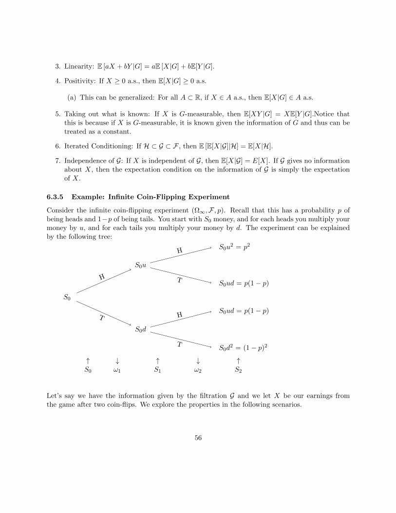
3. Linearity: E [aX + bY |G] = aE [X|G] + bE[Y |G].
4. Positivity: If X ≥ 0 a.s., then E[X|G] ≥ 0 a.s.
(a) This can be generalized: For all A ⊂ R, if X ∈ A a.s., then E[X|G] ∈ A a.s.
5. Taking out what is known: If X is G-measurable, then E[XY |G] = XE[Y |G].Notice thatthis is because if X is G-measurable, it is known given the information of G and thus can betreated as a constant.
6. Iterated Conditioning: If H ⊂ G ⊂ F , then E [E[X|G]|H] = E[X|H].
7. Independence of G: If X is independent of G, then E[X|G] = E[X]. If G gives no informationabout X, then the expectation condition on the information of G is simply the expectationof X.
6.3.5 Example: Infinite Coin-Flipping Experiment
Consider the infinite coin-flipping experiment (Ω∞,F , p). Recall that this has a probability p ofbeing heads and 1−p of being tails. You start with S0 money, and for each heads you multiply yourmoney by u, and for each tails you multiply your money by d. The experiment can be explainedby the following tree:
S0
S0d
S0d2 = (1− p)2T
S0ud = p(1− p)HT
S0u
S0ud = p(1− p)T
S0u2 = p2
H
H
↑ ↓ ↑ ↓ ↑S0 ω1 S1 ω2 S2
Let’s say we have the information given by the filtration G and we let X be our earnings fromthe game after two coin-flips. We explore the properties in the following scenarios.
56
1. G = F0. Recall that F0 = Ω∞, ∅ and thus it literally contains no information. Thus we havethat X is independent of the information in F0. E[X|F0] =E[X]. We can calculate this using thetraditional measures:
E[X] =∑i
xi Pr(X = xi) = S0
(p2u2 + 2p(1− p)ud+ (1− p)2d2
).
2. G = F1. Recall that F1 is the information contained after the first event. Thus we know theresult of the first event, ω1. Thus we can calculate what we would expect X to be given what weknow about the first event. Thus
E[X|F1] =
S0
(pu2 + (1− p)ud
), ω1 = H
S0
(pud+ (1− p)d2
), ω1 = T
.
3. G = F2. Notice that if we have the information of F2, then X is determined (X is G-measurable). Thus
E[X|F2] =
S0u
2, ω1ω2 = HH
S0ud, ω1ω2 = HT or TH
S0d2 ω1ω2 = TT
.
6.4 Martingales
Definition: Take the probability space (Ω,F , p) with the filtration Ft0≤t≤T , and let Mt0≤t≤Tis an adaptive stochastic process w.r.t. Ft. Mt is a martingale if E[Mt|Fs] = Ms for all 0 ≤ s ≤ t.If E[Mt|Fs] ≥ Ms then we call Mt a sub-martingale, while if E[Mt|Fs] ≤ Ms then we call Mt asuper-martingale.
These definitions can be interpreted as follows. If, knowing the value at time s, our best guessfor Mt is that it is the value Ms, then Mt is a martingale. If we assume that it will grow inexpectation in time, it’s a sub-martingale while if we assume that its value will shrink in time, it isa super-martingale.
6.4.1 Example: Infinite Coin-Flipping Experiment Martingale Properties
Looking back at the infinite coin-toss experiment, if Sn is the money we have after event n, then
Sn+1 =
uSn, ωk+1 = H
dSn, ωk+1 = T.
Thus we have that
E[Sn+1|Fn] = puSn + (1− p)dSn = Sn (pu+ (1− p)d) = αSn.
Recalling that Sn is a martingale if we would expect that our value in the future is the same asnow, then
57
1. If α = 1, then Sn is a martingale.
2. If α ≥ 1, then Sn is a sub-martingale.
3. If α ≤ 1, then Sn is a super-martingale.
6.4.2 Example: Brownian Motion
Theorem: A Brownian motion Bt is a martingale.Proof:
E[Bt|Fs] = E[Bt −Bs +Bs|Fs] = E[Bt −Bs|Fs] + E[Bs|Fs] = 0 +Bs = Bs
since on average Bt −Bs = 0.
6.5 Martingale SDEs
Theorem: Take the SDEdXt = a(Xt, t)dt+ b(Xt, t)dWt.
If a(Xt, t) = 0, then Xt is a martingale.Proof: If we take the expectation of the SDE, then we see that
dE[Xt]
dt= a(Xt, t)
and thus if a(Xt, t) = 0, the expectation does not change and thus Xt is a martingale.
6.5.1 Example: Geometric Brownian Motion
Take the stochastic process
Zt = f(Wt, t) = e−θWt− 12θ2t.
Notice using Ito’s Rules that
dZt =∂f
∂tdt+
∂f
∂WtdWt +
1
2
∂2f
∂W 2t
(dWt)2
= −1
2θ2Ztdt− θZtdWt +
1
2θ2Ztdt
= −θZtdWt
since (dWt)2 = dt. Thus since there is no deterministic part, Zt is a martingale. Thus since Z0 = 1,
we get thatE[Zt|Fs] = Zs,
andE[Zt|F0] = 1.
58
6.6 Application of Martingale Theory: First-Passage Time Theory
Take the SDE
dXt = f(Xt, t)dt+
n∑i=1
gi(Xt, t)dWi.
Here we will consider first-passage time problems. These are problems where we start in a setand want to know at what time we he the boundary. Fix x > 0. Let τ = inft ≥ 0 : Xt = xwhich is simply the first time that Xt hits the point x.
6.6.1 Kolmogorov Solution to First-Passage Time
Notice that we can solve for the probability definition using the Forward Kolmogorov Equation
∂ρ(x, t)
∂t= − ∂
∂x[f(x)ρ(x, t)] +
1
2
m∑i=1
∂2
∂x2
[g2i (x)ρ(x, t)
].
Given the problem, we will also have some initial condition ρ(x, 0) = ρ0(x). If we are looking forfirst passage to some point x0, then we put an absorbing condition there ρ(x0, t) = 0. Thus theprobability that you have not hit x0 by the time t is given by the total probability that has notbeen absorbed by the time t, and thus
Pr(t ≥ τ) =
∞−∞
ρ(x, t)dx
to get the cumulative probability distribution
Pr(t ≤ τ) = 1− ∞−∞
ρ(x, t)dx.
Thus the probability density function for τ is simply
fτ (t) =∂
∂t
[ ∞−∞
ρ(x, t)dx
].
This method will always work, though many times the PDE will not have an analytical solution.However, this can always be solved using computational PDE solvers.
6.6.2 Stopping Processes
If Mt is a martingale, then the stopped martingale is defined as
M(t ∧ τ) =
M(t), t ≤ τM(τ), t ≥ τ
59
where M(t ∧ τ) = min(t, τ). This simply the process that we stop once it hits x.Theorem: If Mt is a martingale, then Mt∧τ is a martingale.The proof is straight-forward. Since the stopped martingale does not change after τ , then the
expectation definitely will not change after τ . Since it is a martingale before τ , the expectationdoes not change before τ . Thus Mt∧τ is a martingale.
6.6.3 Reflection Principle
Another useful property is known as the Reflection Principle. Basically, if we look at any Brownianmotion at the time T , there is just as much of a probability of it going up and there is of it goingdown. Thus the trajectory that is reflected after a time τ is just as probable as the non-reflectedpath.
We can formally write the Reflection Principle as
P (τ ≤ t, Bt < x) = P (Bt ≥ x).
This leads to the relation
P (τ ≤ t) = P (τ ≤ t, Bt < x) + P (τ ≤ t, Bt ≥ x)
= 2P (Bt ≥ x)
= 2
∞x
1√2πt
e−u2
2t du.
60
6.7 Levy Theorem
Theorem: Levy Theorem. Take (Ω,F , p). If W (t) is a martingale under p and dW (t)×dW (t) =dt, then W (t) is Brownian Motion.
We state this without proving it since this takes a lot more detailed treatment of Brownianmotion.
6.8 Markov Processes and the Backward Kolmogorov Equation
6.8.1 Markov Processes
Take 0 ≤ t0 < t and let h(y) be a function. Define
Et0,x [h(x(t)] = v(t0, x)
as the expectation of h(x(t)) given that x(t0) = x.Definition: Take the random variable x. If
E0,ζ [h(x(t)|Ft0 ] = Et0,x [h(x(t)] = v(t0, x),
then we say x satisfies the Markov property and is thus a Markov process. Another way of statingthis is that
E [f(Xt)|Fs] = E [f(Xt)|σ(Xs)] ,
orP (xt ∈ A|Fs) = P (xt ∈ A|xs).
Intuitively, this property means that the total information for predicting the future of xt is com-pletely encapsulated by the current state xt.
6.8.2 Martingales by Markov Processes
Take the SDE dXt = a(Xt)dt+ b(Xt)dWt.Theorem: Xt is a Markov Process.Theorem: Given Et0,x [h(x(t)] = v(t0, x), v(x, t)0≤t≤T is a martingale w.r.t. Ft.Proof: Look at E [v(x, t)|Fs] for 0 < s ≤ t. Notice
E [v(x(t), t)|Fs] = E[Et0,x [h(x(t))|Ft] |Fs
]= E [h(x(t))|Fs] = v(x(s), s)
since Fs ⊂ Ft. Thus v is a martingale.
61
6.8.3 Transition Densities and the Backward Kolmogorov
We can use this in the following proof. Notice that
dv =∂v
∂tdt+
∂v
∂xdx+
1
2
∂2v
∂x2(dx)2
=∂v
∂tdt+
∂v
∂x(a(Xt)dt+ b(Xt)dWt) +
1
2
∂2v
∂x2b2(x(t), t)dt
=
(∂v
∂t+ a(Xt)
∂v
∂x+
1
2b2(x(t), t)
∂2v
∂x2
)dt+ b(Xt)
∂v
∂xdWt.
Since v is a martingale, the deterministic part must be zero. Thus we get the equation
∂v
∂t+ a(Xt)
∂v
∂x+
1
2b2(x(t), t)
∂2v
∂x2= 0.
We can solve this using the initial condition v(x, T ) = h(x) to solve for v(x(t), t).Define the transition density function as
ρ(t0, t, x, y)dy = P x(t) ∈ (y, y + dy)|x(t0) = x
which is the probability of transitioning from x to y between t0 and t. Notice that the probabilityof transitioning from h(x) to h(y) from the time t to T is
v(x, t) = Et,x [h(x(T ))] =
∞−∞
ρ(t, T, x, y)h(y)dy.
Now suppose we know h(z) = δ(x− y), meaning that we know that the trajectory ends at y. Thus
v(x, t) =
∞−∞
ρ(t, T, x, y)δ(x− y)dy
= ρ(t, T, x, y).
Thus we plug this into the PDE for v to get
∂ρ
∂t+ a(x(t), t)
∂ρ
∂x+
1
2b2(x(t), t)
∂2ρ
∂x2= 0.
with the terminal condition ρ(T, x) = δ(x− y) where y is the place the trajectory ends. Thus thisequation, the Kolmogorov Backward Equation, tells us that if we know the trajectory ends at y ata time T , what is the probability that it was x and a time t < T . Notice that this is not the sameas the Kolmogorov Forward Equation. This is because diffusion forward does not equal diffusionbackwards. For example, say you place dye in water. It will diffuse to spread out uniformly aroundthe water. However, if we were to play that process in reverse it would look distinctly different.
62
6.9 Change of Measure
The purpose of the change of measure is that is can greatly simplify equations by taking outdeterministic parts and making random variables into martingales. This will be crucial whenunderstanding the solution to the Black-Scholes equation.
6.9.1 Definition of Change of Measure
Take the probability space (Ω,F , p). Let z be a non-negative random variable s.t. E [z] = 1. Definethe new measure p as
p(A) =
Azdp.
Thus for any random variable x in the probability space (Ω,F , p) we get that
E [x] = E [xz]
and if z > 0 a.s. we get
E [x] = E[xz
]where E is the expectation using the measure p.
Definition: p and p are equivalent if they agree on which sets have probability zero.Corollary: They agree on which events will not occur a.s.Theorem: Radon-Nikodym Theorem. Let p and p be equivalent measures on (Ω,F). There
exists a random variable z > 0 a.s. such that p(A) =A zdp where z =
dp
dp. We call
dp
dpthe
Radon-Nikodym derivative.
6.9.2 Simple Change of Measure Example
Take (Ω,F , p) and let X be a standard normal random variable under p. Define y = x+ θ. Noticethat under p, y ∼ N(θ, 1). However, if we define
z(ω) = e−θX(ω)− θ2
2
and define
p(A) =
Azdp,
in this reweighing of the probability space y is standard normal. This is because by definition thepdf of y using the measure p is
f(y) = z(θ)N(x+ θ, 1)
= eθx−θ2/2e−(x+θ)2/2 1√
2π
=1√2πe−x
2/2 ∼ N(0, 1)
63
6.9.3 Radon-Nikodym Derivative Process
Take any random variable X. Using this Radon-Nikodym derivative and a filtration, we can use itto define a unique process with no deterministic part Z, and use this random variable to define ameasure p to transform one stochastic process to another.
Definition: Take(Ω, F, P ) with Ft as a filtration of this space up to t with 0 ≤ t ≤ T where T
is some fixed finish time. Let ζ = dPdP and satisfy the conditions required to be a Radon-Nikodym
derivative. We can define a Radon-Nikodym derivative process (RNDP) Zt as
Zt = E[ζ|Ft].
Notice that
1. Z(t) is a martingale.
2. If we let y be an Ft-meausrable random variable, then
E[y] = E[yZt] = E [yE[ζ|Ft]] = E [E[yζ|Ft]] = E[yζ],
and
E[y|Fs] =E[yZt|Fs]
Zs,
for 0 ≤ s ≤ t ≤ T .
6.9.4 Girsanov Theorem
Using the change of measure determined by the RNDP, we can always construct a Brownian motionfrom an adapted stochastic process. This is known as Girsanov Theorem.
Theorem: Girsanov Theorem. Let Wt be a Brownian motion in (Ω, F, P ) and Ft be afiltration with 0 ≤ t ≤ T . Let θ(t) be an adapted stochastic process on Ft. Define
Z(t) = e− t0 θ(u)dW (u)− 1
2
t0 θ
2(u)du
Wt = Wt +
t
0θ(u)du
dWt = dWt + θ(t)dt
Define the probability measure p using Z as
p(A) =
AZdp.
Then the following statements hold:
1. E [Z] = 1
64
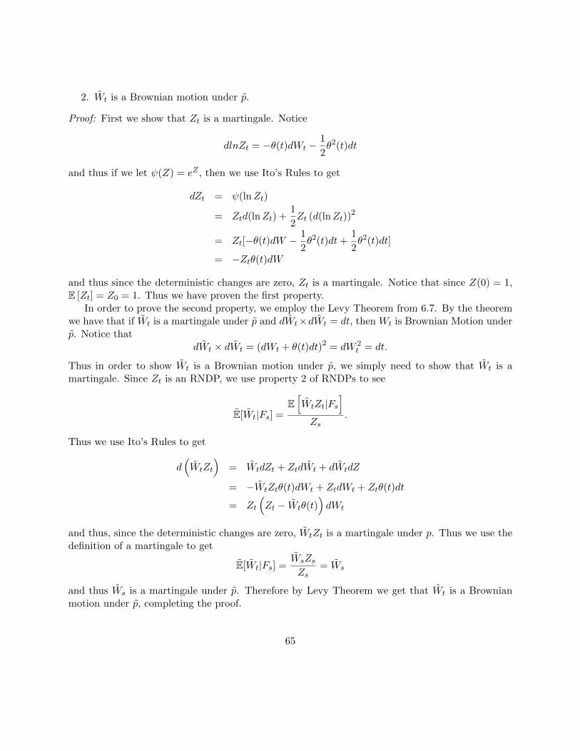
2. Wt is a Brownian motion under p.
Proof: First we show that Zt is a martingale. Notice
dlnZt = −θ(t)dWt −1
2θ2(t)dt
and thus if we let ψ(Z) = eZ , then we use Ito’s Rules to get
dZt = ψ(lnZt)
= Ztd(lnZt) +1
2Zt (d(lnZt))
2
= Zt[−θ(t)dW −1
2θ2(t)dt+
1
2θ2(t)dt]
= −Ztθ(t)dW
and thus since the deterministic changes are zero, Zt is a martingale. Notice that since Z(0) = 1,E [Zt] = Z0 = 1. Thus we have proven the first property.
In order to prove the second property, we employ the Levy Theorem from 6.7. By the theoremwe have that if Wt is a martingale under p and dWt×dWt = dt, then Wt is Brownian Motion underp. Notice that
dWt × dWt = (dWt + θ(t)dt)2 = dW 2t = dt.
Thus in order to show Wt is a Brownian motion under p, we simply need to show that Wt is amartingale. Since Zt is an RNDP, we use property 2 of RNDPs to see
E[Wt|Fs] =E[WtZt|Fs
]Zs
.
Thus we use Ito’s Rules to get
d(WtZt
)= WtdZt + ZtdWt + dWtdZ
= −WtZtθ(t)dWt + ZtdWt + Ztθ(t)dt
= Zt
(Zt − Wtθ(t)
)dWt
and thus, since the deterministic changes are zero, WtZt is a martingale under p. Thus we use thedefinition of a martingale to get
E[Wt|Fs] =WsZsZs
= Ws
and thus Ws is a martingale under p. Therefore by Levy Theorem we get that Wt is a Brownianmotion under p, completing the proof.
65
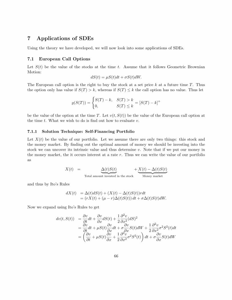
7 Applications of SDEs
Using the theory we have developed, we will now look into some applications of SDEs.
7.1 European Call Options
Let S(t) be the value of the stocks at the time t. Assume that it follows Geometric BrownianMotion:
dS(t) = µS(t)dt+ σS(t)dW.
The European call option is the right to buy the stock at a set price k at a future time T . Thusthe option only has value if S(T ) > k, whereas if S(T ) ≤ k the call option has no value. Thus let
g(S(T )) =
S(T )− k, S(T ) > k
0, S(T ) ≤ k= [S(T )− k]+
be the value of the option at the time T . Let v(t, S(t)) be the value of the European call option atthe time t. What we wish to do is find out how to evaluate v.
7.1.1 Solution Technique: Self-Financing Portfolio
Let X(t) be the value of our portfolio. Let we assume there are only two things: this stock andthe money market. By finding out the optimal amount of money we should be investing into thestock we can uncover its intrinsic value and thus determine v. Note that if we put our money inthe money market, the it occurs interest at a rate r. Thus we can write the value of our portfolioas
X(t) = ∆(t)S(t)︸ ︷︷ ︸Total amount invested in the stock
+X(t)−∆(t)S(t)︸ ︷︷ ︸Money market
and thus by Ito’s Rules
dX(t) = ∆(t)dS(t) + (X(t)−∆(t)S(t))rdt= (rX(t) + (µ− r)∆(t)S(t)) dt+ σ∆(t)S(t)dW.
Now we expand using Ito’s Rules to get
dv(t, S(t)) =∂v
∂tdt+
∂v
∂xdS(t) +
1
2
∂2v
∂x2(dS)2
=∂v
∂tdt+ µS(t)
∂v
∂xdt+ σ
∂v
∂xS(t)dW +
1
2
∂2v
∂x2σ2S2(t)dt
=
(∂v
∂t+ µS(t)
∂v
∂x+
1
2
∂2v
∂x2σ2S2(t)
)dt+ σ
∂v
∂xS(t)dW
66
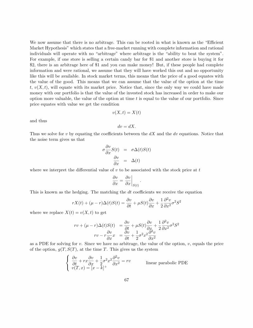
We now assume that there is no arbitrage. This can be rooted in what is known as the “EfficientMarket Hypothesis” which states that a free-market running with complete information and rationalindividuals will operate with no “arbitrage” where arbitrage is the “ability to beat the system”.For example, if one store is selling a certain candy bar for $1 and another store is buying it for$2, there is an arbitrage here of $1 and you can make money! But, if these people had completeinformation and were rational, we assume that they will have worked this out and no opportunitylike this will be available. In stock market terms, this means that the price of a good equates withthe value of the good. This means that we can assume that the value of the option at the timet, v(X, t), will equate with its market price. Notice that, since the only way we could have mademoney with our portfolio is that the value of the invested stock has increased in order to make ouroption more valuable, the value of the option at time t is equal to the value of our portfolio. Sinceprice equates with value we get the condition
v(X, t) = X(t)
and thusdv = dX.
Thus we solve for v by equating the coefficients between the dX and the dv equations. Notice thatthe noise term gives us that
σ∂v
∂xS(t) = σ∆(t)S(t)
∂v
∂x= ∆(t)
where we interpret the differential value of v to be associated with the stock price at t
∂v
∂x=∂v
∂x
∣∣∣∣S(t)
.
This is known as the hedging. The matching the dt coefficients we receive the equation
rX(t) + (µ− r)∆(t)S(t) =∂v
∂t+ µS(t)
∂v
∂x+
1
2
∂2v
∂x2σ2S2
where we replace X(t) = v(X, t) to get
rv + (µ− r)∆(t)S(t) =∂v
∂t+ µS(t)
∂v
∂x+
1
2
∂2v
∂x2σ2S2
rv − r ∂v∂xx =
∂v
∂t+
1
2σ2x2 ∂
2v
∂x2
as a PDE for solving for v. Since we have no arbitrage, the value of the option, v, equals the priceof the option, g(T, S(T ), at the time T . This gives us the system ∂v
∂t+ rx
∂v
∂x+
1
2σ2x2 ∂
2v
∂x2= rv
v(T, x) = [x− k]+linear parabolic PDE
67
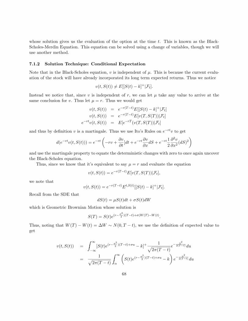
whose solution gives us the evaluation of the option at the time t. This is known as the Black-Scholes-Merdin Equation. This equation can be solved using a change of variables, though we willuse another method.
7.1.2 Solution Technique: Conditional Expectation
Note that in the Black-Scholes equation, v is independent of µ. This is because the current evalu-ation of the stock will have already incorporated its long term expected returns. Thus we notice
v(t, S(t)) 6= E[[S(t)− k]+|Ft].
Instead we notice that, since v is independent of r, we can let µ take any value to arrive at thesame conclusion for v. Thus let µ = r. Thus we would get
v(t, S(t)) = e−r(T−t)E[[S(t)− k]+|Ft]v(t, S(t)) = e−r(T−t)E[v(T, S(T ))|Ft]
e−rtv(t, S(t)) = E[e−rT (v(T, S(T ))|Ft]
and thus by definition v is a martingale. Thus we use Ito’s Rules on e−rtv to get
d(e−rtv(t, S(t))) = e−rt(−rv +
∂v
∂t]dt+ e−rt
∂v
∂xdS + e−rt
1
2
∂2v
∂x2(dS)2
)and use the martingale property to equate the deterministic changes with zero to once again uncoverthe Black-Scholes equation.
Thus, since we know that it’s equivalent to say µ = r and evaluate the equation
v(t, S(t)) = e−r(T−t)E[v(T, S(T ))|Ft],
we note thatv(t, S(t)) = e−r(T−t)Et,S(t)[[S(t)− k]+|Ft].
Recall from the SDE thatdS(t) = µS(t)dt+ σS(t)dW
which is Geometric Brownian Motion whose solution is
S(T ) = S(t)e(r−σ2
2)(T−t)+σ(W (T )−W (t).
Thus, noting that W (T ) −W (t) = ∆W ∼ N(0, T − t), we use the definition of expected value toget
v(t, S(t)) =
∞−∞
[S(t)e(r−σ2
2)(T−t)+σu − k]+
1√2π(T − t)
e− u2
2(T−t)du
=1√
2π(T − t)
∞α
(S(t)e(r−σ
2
2)(T−t)+σu − k
)e− u2
2(T−t)du
68
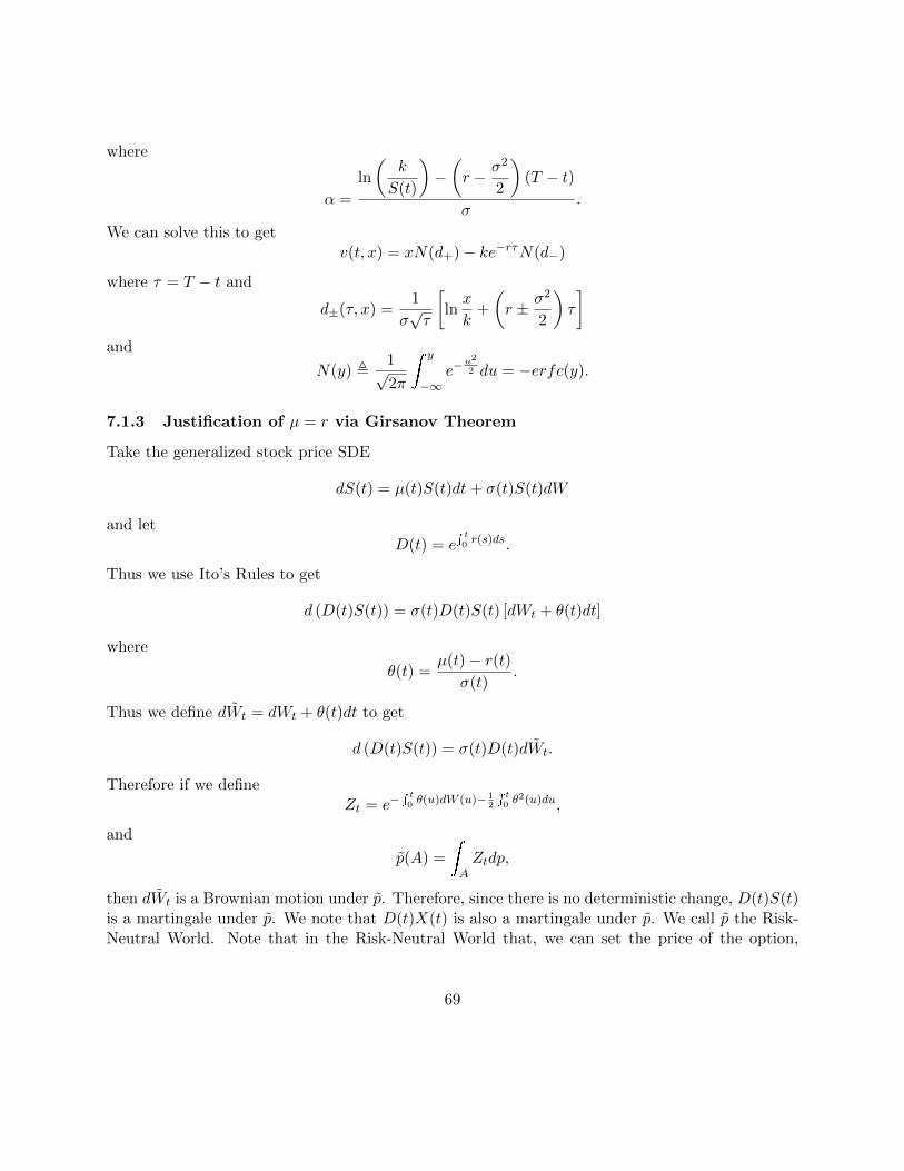
where
α =
ln
(k
S(t)
)−(r − σ2
2
)(T − t)
σ.
We can solve this to getv(t, x) = xN(d+)− ke−rτN(d−)
where τ = T − t and
d±(τ, x) =1
σ√τ
[lnx
k+
(r ± σ2
2
)τ
]and
N(y) ,1√2π
y
−∞e−
u2
2 du = −erfc(y).
7.1.3 Justification of µ = r via Girsanov Theorem
Take the generalized stock price SDE
dS(t) = µ(t)S(t)dt+ σ(t)S(t)dW
and letD(t) = e
t0 r(s)ds.
Thus we use Ito’s Rules to get
d (D(t)S(t)) = σ(t)D(t)S(t) [dWt + θ(t)dt]
where
θ(t) =µ(t)− r(t)
σ(t).
Thus we define dWt = dWt + θ(t)dt to get
d (D(t)S(t)) = σ(t)D(t)dWt.
Therefore if we defineZt = e−
t0 θ(u)dW (u)− 1
2
t0 θ
2(u)du,
and
p(A) =
AZtdp,
then dWt is a Brownian motion under p. Therefore, since there is no deterministic change, D(t)S(t)is a martingale under p. We note that D(t)X(t) is also a martingale under p. We call p the Risk-Neutral World. Note that in the Risk-Neutral World that, we can set the price of the option,
69
discounted by D(t), as the expectation conditioned on the totality of information that we have.Thus for V (S(T ), T ) as the payoff of a derivative for a security for stock S(T ) at time T , we get
D(t)V (S(t), t) = E [D(t)V (S(t), t)|Ft] .
This is an equivalent expression as the conditional expectation from before, saying that we can letµ = r because this is simply a change of measure into the Risk-Neutral World.
7.2 Population Genetics
We consider a new case study involving population genetics under the Wright-Fisher model. TheWright-Fisher model is a discrete stochastic model of genetic variance which was first introduced toformally develop the ideas of genetic drift. We will start by considering the classical Wright-Fishermodel and show how it can be approximated using SDEs. This will give us an intuitive way ofgeneralizing and simulating Wright-Fisher models in a way that is useful for applications. Thistype of analysis is taken from Richard Durrett’s Probability Models for DNA.
7.2.1 Definitions from Biology
First we will introduce some definitions from biology. A gene locus is simply a location on achromosome or a portion of a chromosome. It can represent a gene, a SNP (single base pairpolymorphism) or simply a location. An allele is one of a number of alternative forms of the locus.A dominant allele is usually capitalized. For human and other diploid animals, there are typicallytwo alleles of paternal and maternal origin. A genotype is the genetic makeup of an individual.In this case it will denote the types of alleles an individual individual carries. For example, if theindividual has one dominant allele and one recessive allele, its genotype is Aa. Having the samepair of alleles is called homozygous while having different alleles is called heterozygous. A mutationis a random genetic change. Here we refer to it as the random spontaneous change of one allele toanother. Fitness is the measure of survivability and ability to reproduce of an individual possessinga certain genotype (this is wrong for many philosophical / scientific reasons, but we can take thisas a working definition since this is a major topic worth its own book) . Neutral evolution is thecase where all genotypes of interest have the same fitness. This implies that there is no selectionfrom such genetic variations and all change is inherently random.
7.2.2 Introduction to Genetic Drift and the Wright-Fisher Model
Here we introduce the Wright-Fisher model. Consider a model with the following assumptions:
1. There is a population with finite size N .
2. The size of the population is constant throughout evolution.
3. There are discrete, non-overlapping generations.
70
4. Mating is completely random and is determined by random sampling with replacements. Thismeans any individual can randomly give rise to 0, 1, . . . many offsprings.
From this, the time evolution of the Wright-Fisher model is defined as:
1. At generation 0, there are 2N alleles some A, some a.
2. At generation 1, each A or a allele from generation 0 may result in one, more or zero copiesof that allele.
The following theorem holds:Theorem: Genetic Drift. Because the population size is finite and fixed, due to uneven
passing of alleles by chance, eventually there will be only one allele, A or a, left. This is known asGenetic Drift.
Notice the implication of the theorem. This means that, even in the absence of selection, youcan have alleles fix in the population and thus have a form of evolution occur! We can intuitivelyunderstand this as simply due to first-passage problems.
7.2.3 Formalization of the Wright-Fisher Model
Let us characterize the Wright-Fisher model in probabilistic terms. Let Xn be the total number ofA alleles at generation n. Considering that there are a total of 2N alleles in any given generation,we can define Pn = Xn
2N to be the percentage of alleles that are A. Let X0 be some known initialcondition. Because there are 2N independent alleles that could be passed and the probability ofgenerating an A allele at generating n is Pn−1 (because of sampling with replacement), we can derivethe distribution for Xn using indicator functions. Order the alleles in the population. Let Xn,i be1 if the ith allele is an A and 0 if the ith allele is a 0. Since we are sampling with replacement, thechoice of allele i is independent of the choice of allele j for any i 6= j. Thus each Xn,i ∼ Bern(Pn−1),that is each is a Bernoulli random variable with probability of heads equal to Pn−1. Therefore,since Xn =
∑iXn,i and each Xn,i are independent, Xn is modeled by the result of 2N coin-flips
each with a probability Pn−1 of heads. Thus
Xi ∼ Bin(2N,Pi−1),
which makes
Pr(Xk = k, 0 ≤ k ≤ 2N) =
(2Nk
)P kn−1 (1− Pn−1)2N−k .
Thus we can show thatE [Xn|Xn−1] = 2NPn−1 = Xn−1
which implies Xn is a martingale. Also
V [Xn] = 2NPn−1(1− Pn−1).
71
Notice that we can think of this process as some form of a random walk for Xn with probability ofgoing right as Pn−1. One can rigorous show then that for the 1-dimension random walk of this sort
limn→∞
Pn = 0 or 1
which means that the process will fix to one of the endpoints in a finite time. Since Xn is amartingale, we note that
limn→∞
E [Xn] = X0,
which means
Pr(X∞ = 2N) ∗ (2N) + Pr(X∞ = 0) ∗ 0 = X0
and thus by dividing by 2N we get
Pr(X∞ = 2N) = P0.
7.2.4 The Diffusion Generator
If we assume N is large, then it is reasonable to assume that the gene frequencies Pn will change ina manner that is almost continuous and thus can be approximated by an SDE. Consider an SDEof the form
dXt = a(x)dt+√b(x)dWt
with the initial condition X0 = x. Applying Ito’s rule gives us
df(Xt) =df
dXdXt +
1
2
d2f
dX2(dXt)
2 ,
=df
dXa(x)dt+
df
dX
√b(x)dW +
1
2
d2f
dX2b(x)dt.
Writing fX = ∂f∂X and fXX = ∂2f
∂X2 , we get that
E [f(Xt)]
dt= fXa(x) +
1
2fXXb(x).
Thus we define L to be the operator
Lf =E [f(Xt)]
dt= fXa(x) +
1
2fXXb(x).
L is known as the diffusion generator. If we let f(x) = x then
Lf = a(x) =dE [f(x)]
dt
72
where a(x) defines the infinitesimal mean changes. If we define f(y) = (y − x)2 for a fixed x, then
b(x) =d
dtE[(Xt − x))2
]makes b(x) define the infinitesimal variance. Therefore, we can generally relate discrete stochasticprocesses to continuous stochastic processes by defining the SDE with the proper a and b suchthat the mean and variance match up. This can formally be shown to be the best continuousapproximation to a discrete Markov process using the Kolmogorov Forward Equation.
7.2.5 SDE Approximation of the Wright-Fisher Model
Recall that in the Wright-Fisher Model we have that
V [Xn] = 2NPn−1(1− Pn−1).
Notice too then thatV [Pn] = Pn−1(1− Pn−1).
BecauseE [Xn|Xn−1] = Xn−1
we get thatdE [Xn]
dt= 0.
This means that we define the SDE approximation of the Wright-Fisher model to be the one thatmatches the mean and variances, that is
dXt =√Xt (1−Xt)dWt.
Notice that this approximation converges as N →∞.
7.2.6 Extensions to the Wright-Fisher Model: Selection
Now we extend the Wright-Fisher model to incorporate more of the population dynamics. Forexample, assume that there is selection. Assume that the fitness of A is 1 and that the fitness of ais 1− s for some constant s. We define this using a re-sampling idea. We say that if A is sampled,will accept it with probability 1, while if a is sampled, we will accept it with a probability 1 − s.This means that the probability of choosing A is
Xn−1
Xn−1 + (1−Xn−1)(1− s).
Assuming s is small, the probability of choosing A is
≈ Xn−1
1− (1−Xn−1)s= Xn−1
(1 + (1−Xn−1) s+O(s2)
)73
and thus∆Xn = Xn −Xn−1 ≈ Xn−1(1−Xn−1)s.
Therefore we makedE [Xn]
dt= sXn−1 (1−Xn−1) .
To make this continuous we note
dE [Pn]
dt=
s
2NPn−1 (1− Pn−1) .
= γPn−1 (1− Pn−1)
where γ = s2N . Therefore we make this continuous by matching the diffusion operator as
L = γx(1− x)d
dx+
1
2x(1− x)
d2
dx2
and thus we approximate the Wright-Fisher model with selection as the SDE
dXt = γXt (1−Xt) dt+√Xt (1−Xt)dWt
when N is large.
7.2.7 Extensions to the Wright-Fisher Model: Mutation
Let µ1 = β1
2N be the chance of a allele randomly changing to A allele, and µ2 = β2
2N be the chanceof the reverse mutation. One can derive the differential generator for this process to be
L = (γx(1− x) + β1 (1− x) + β2x)d
dx+
1
2x(1− x)
d2
dx2.
Therefore the best SDE approximation to the Wright-Fisher Model with selection and mutation is
dXt = (γx(1− x) + β1 (1− x) + β2x) dt+√Xt (1−Xt)dWt.
7.2.8 Hitting Probability (Without Mutation)
Let h(t) = Pr(τ ≤ t) where τ = inft X(t) = a. For example, a = 1 would mean that τ is the timefor fixation by A. If there is no selection in the model, then h(t) is a martingale and thus
E [h(t)|Fs] = h(s)
and therefore, in the limit as t→ 0,
74
h(x) =
1
0Pr(Xt = y|X0 = x)h(y)dy
1
0δ(x− y)h(y)dy =
1
0Pr(Xt = y|X0 = x)h(y)dy
0 =
1
0[Pr(Xt = y|X0 = x)− δ(x− y)]h(y)dy.
This, in the limit as t→ 0,
Pr(Xt = y|X0 = x)− δ(x− y)→ ∂ρ
∂t
Recall that from the Kolmogorov Forward Equation that
∂ρ
∂t=∂(aρ)
∂x+
1
2b2∂2ρ
∂x2.
Thus
0 =
1
0
∂ρ
∂th(y)dy
0 =
1
0
[−∂(aρ)
∂x+
1
2b2∂2ρ
∂x2
]h(y)dy
To solve this we use integration by parts to get the PDE
Lh = 0
h(a) = 1
h(b) = 0
where
L = a(x)d
dx+
1
2b(x)
d2
dx.
To solve for the probability density function of the first-passage time, define ψ = dhdx and thus
ψ′ = −a(x)b(x) . Therefore we get
ψ(x) = ψ(0)e−
x0a(y)b(y)
dy
and
h(x) =
x
0ψ(y)dy.
This is expanded in the book by Kimora and Crow.
75
7.2.9 Understanding Using Kolmogorov
Notice that, given the SDE, we can understand the dynamics using the Kolmogorov equation.The fixation time distribution can be calculated by using the forward Kolmogorov with absorbingconditions at 0 and 1, that is ρ(0, t) = ρ(1, t) and thus we can solve for the fixation times usingthe first-passage time distributions as examined in 6.6.1. Also note that when we have mutation,there exists a non-trivial steady state distribution. Using the Kolmogorov equation, we can solvefor this steady state distribution as the distribution π s.t. ∂π
∂t = 0 and thus
0 = − ∂
∂x[a(x)π(x, t)] +
1
2
∂2
∂x2
[b2(x)π(x, t)
].
For the Wright-Fisher model with selection and mutation, we note that this can be solved so that
π(x) = x2β1−1(1− x)2β2−1 = Γ(2β − 1).
Notice that this solution is only valued when β1, β2 > 12 , giving us the necessary and sufficient
conditions for a non-trivial steady state.
7.3 Stochastic Control
The focus of this lecture will be on stochastic control. We begin by looking at optimal control inthe deterministic case.
7.3.1 Deterministic Optimal Control
Suppose you have a deterministic ODE
x = F (x(t), u(t))
where x(t) is the state variable and u(t) is the control variable. We wish to apply optimal controlover a fixed time period [0, T ] such that
V (x(t), t) = minu
T
0C[x(t), u(t)]dt+D[x(T )]
where C is the cost function, D is the terminal cost, and V (x(t), t) is the optimal or minimal cost ata time t. Thus what we are looking to do is, given some cost function C, we are looking to minimizethe total cost. Let’s say for example that we want to keep x at a value c, but sending control signalscosts some amount α. Thus an example could be that C(x(t), u(t)) = (x(t)− c)2 + αu(t). Whatwe want to do is solve for the best u(t).
76
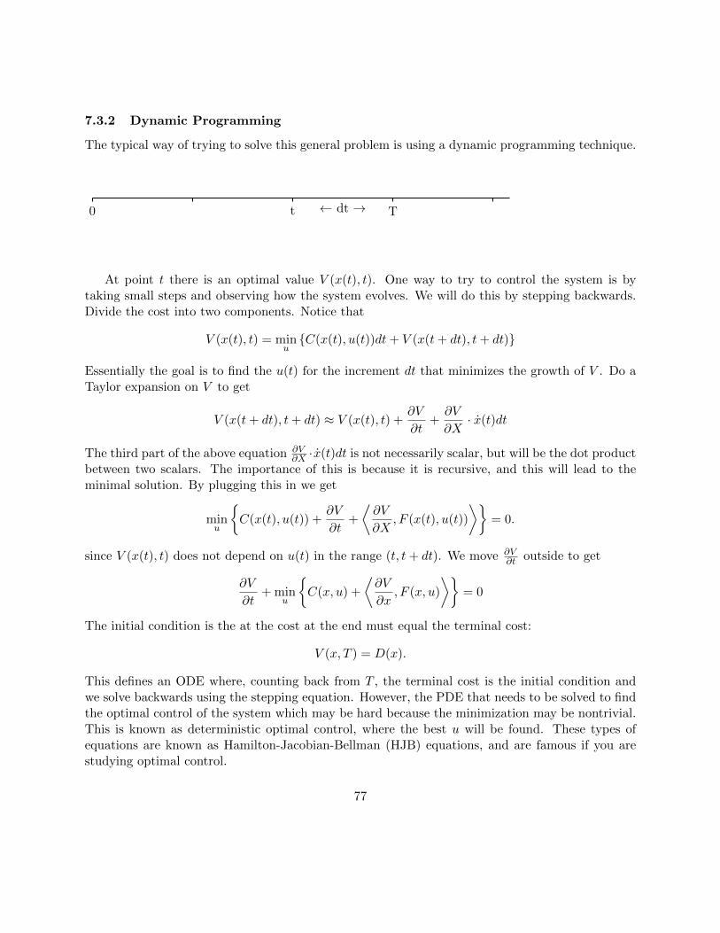
7.3.2 Dynamic Programming
The typical way of trying to solve this general problem is using a dynamic programming technique.
0 t T← dt →
At point t there is an optimal value V (x(t), t). One way to try to control the system is bytaking small steps and observing how the system evolves. We will do this by stepping backwards.Divide the cost into two components. Notice that
V (x(t), t) = minuC(x(t), u(t))dt+ V (x(t+ dt), t+ dt)
Essentially the goal is to find the u(t) for the increment dt that minimizes the growth of V . Do aTaylor expansion on V to get
V (x(t+ dt), t+ dt) ≈ V (x(t), t) +∂V
∂t+∂V
∂X· x(t)dt
The third part of the above equation ∂V∂X ·x(t)dt is not necessarily scalar, but will be the dot product
between two scalars. The importance of this is because it is recursive, and this will lead to theminimal solution. By plugging this in we get
minu
C(x(t), u(t)) +
∂V
∂t+
⟨∂V
∂X,F (x(t), u(t))
⟩= 0.
since V (x(t), t) does not depend on u(t) in the range (t, t+ dt). We move ∂V∂t outside to get
∂V
∂t+ min
u
C(x, u) +
⟨∂V
∂x, F (x, u)
⟩= 0
The initial condition is the at the cost at the end must equal the terminal cost:
V (x, T ) = D(x).
This defines an ODE where, counting back from T , the terminal cost is the initial condition andwe solve backwards using the stepping equation. However, the PDE that needs to be solved to findthe optimal control of the system which may be hard because the minimization may be nontrivial.This is known as deterministic optimal control, where the best u will be found. These types ofequations are known as Hamilton-Jacobian-Bellman (HJB) equations, and are famous if you arestudying optimal control.
77
7.3.3 Stochastic Optimal Control
Now we look at the same problem where the underlying process is the stochastic process
dXt = b(xt, ut)dt+ σ(xt, ut)dWt.
Let Xt ∈ Rn and Wt be an m-dimensional Brownian motion. For this to work, we need σ ∈ Rn×m.Define the value equation as the minimum expected cost, that is
V (x(t), t) = minuE
[ T
tC(X(t), u(t))dt+D[X(T )]
]What type of control is being used? That is the question that needs to be addressed, because thereare many types of controls:
1. Open Loop Control (Deterministic Control).
Suppose u(t, ω) = u(t). This case has no random events and thus it will be deterministiccontrol (open looped control).
2. Open Looped Control (Feedback Control).
Suppose Ut is Mt-adapted, where Mt is the σ-algebra generated by Xs, 0 ≤ s ≤ t . Essentiallyfor this σ-algebra you have all the information about the trajectory from 0 up to a certaintime point, the history must be known.
3. Markov Control
U(t, ω) = u0(t, xt(ω)). Markov control uses less control than the open looped control. It onlyuses what is current, there is nothing beyond that. This is commonly used in programmingapplications because only the last state needs to be saved, leading to iterative solutions thatdo not require much working memory or RAM. An example of where this would be used is acontrol theory about robots. The robot has to decide to walk or stop, and this decision onlydepends on the current state.
These types of controls explain what type of information is allowed to be used. Regardless, wesolve the problem using dynamic programming but this time we use the stochastic Taylor seriesexpansion:
V (x(t+ dt), t+ dt) =∂V
∂t· dt+
∂V
∂x· dX(t) +
1
2(dxt)
T ∂2V
∂x2(dxt)
where ∂2V∂x2 is the Hessian of V . Thus
V (x(t+dt), t+dt) = V (x(t), t)+∂V
∂tdt+
⟨∂V
∂x, b(xt, ut)
⟩dt+
⟨∂V
∂x, σ(xt, ut)dBt
⟩+
1
2
∑i,j
aij∂2V
∂xi∂xj
whereaij = (σσT )ij .
78
After obtaining the expectation we solve as before to get
∂V
∂t+ min
u
C(x, u) + 〈∂V∂x
, b(xt, ut)〉+1
2
∑ij
aij∂2V
∂xi∂xj
= 0
with the same initial (final) condition
V (x, T ) = D(x).
Whether or not the solution exists, or is unique are hard questions. In general the goal is a practicalsolution to the HJB equations. This type of equation does not necessarily have an analyticalsolution. Though caution needs to be exercised as numerical solutions have issues as well. Forexample, how could one find the u that minimize this? Some form of the calculus of variations?There is no clear way of how to do this.
7.3.4 Example: Linear Stochastic Control
SupposedXt = (HtXt +MtUt)dt+ σtdWt
wherex0 = x, t ≥ 0. Ht ∈ Rn/n, Ut ∈ Rk,
σtRn×m, Mt ∈ Rn×k.
This minimizes u over the expectation,
V a(x, 0) = Ex,0 T
0(xTt CtXt + uTt Dtut)dt+XT
T RXT
where Ct are the costs of controlling at t and Dt is the terminal cost. Try to make the u small. Wedenote
ψ(t, x) = minuV u
Using s as the time stand-in variable, we plug the equation into the HJB equation to get
∂ψ
∂s+ min
u
xTCsX + uTPsv +n∑i=1
(Hsx+Ms)i∂ψ
∂xi+
1
2
∑ij
(σsσTs )ij
∂2ψ
∂xi∂xj
= 0
To solve this, try the solutionψ(x, t) = XT
t Stxt + at
where St is positive semi-definite. Thus we get
xT Stx+ at + minu
xTCtx+ V TDtv + vT+ < Htx+Mtv, 2Stx > +∑ij
(σsσTs )ij(St)ij = 0
79
xStx+ at + minu
xT ctx+ V TDtv+ < Htx+Mtvm2S)tx > tr[(σtσ
Tt )St]
= 0
We note that the optimal u isu∗ = −D−1
t MTt Stx.
Plugging in this we solve to
xT (s+ Ct − StMtD−1t MT
t St + 2HTt St)x+ at + tr(σσTS)t = 0.
By matching coefficients, we get the equations
St + Ct − StMtD−1t MT
t St + 2HTt St = 0 ST = R
at = −tr(σσT s)t, aT = 0
The first equation is called a Ricarti equation.
St + StAtSt +BtSt + Ct = 0
These two equations give you St and at such that we arrive at the optimal value.
7.4 Stochastic Filtering
The general problem involves a system of equations
(System) dXt = b(t, xt)dt+ σ(t, xt)dUt
(Observations) dZt = Ct, xt)dt+ γ(t, xt)dVt
Ut : p-dim Brownian motion
Vt : r-dim Brownian motion
where Xt is the state, Zt is the observation, and Ut and Vt are two independent Brownian motions.Assume F , G, C, D are bounded on bounded intervals, Z0 = 0.
In this problem, we seek to estimate the value of the system X at a future time t based on theobservations U up to the present time s < t, that is, conditional on Gt, the σalgebra generated byZs0≤s≤t .
7.4.1 The Best Estimate: E [Xt|Gt]
First you cannot disrespect the intuitive argument. The intuitive argument is that the best predic-tion is to find the value you would expect given all of the information you have. The informationyou have is Gt, and so the best prediction given the totality of information is E [Xt|Gt].
80
More formally, we take that the best estimate based on the observations would be a functionthat only needs to use the information, implying that X() is Gt-measurable. We define the bestestimate as the one that minimizes the Euclidean distance, that is
X() = infY ∈K
E[(Xt − Y )2
]where
Kt :=Y : Ω→ Rn : Y ∈ L2(P ) and Y is Gt-measurable
.
with L2(P ) being the set of L2integrable functions by the measure P .Theorem: Let Gt ⊂ Ft be a sub-σ-algebra and let X ∈ L2(p) be Ft-measurable. Let N =
Y ∈ L2(P ) : Y isGt-measurable
. It follows that
PN (Xt) = E [Xt|Gt]
where PN is the orthogonal projection of X onto N .Proof: To prove that PN (Xt) = E [Xt|Gt], we simply need to show it satisfies the two properties
of the conditional expectation. Notice that it is trivial that PN (Xt) is Gt-measurable since everyX ∈ N is Gt-measurable. Thus we just need to check the Partial Averaging Property. Since PN isan orthogonal projection onto N , we get that X − PN (X) is orthogonal to N . Now take IA ∈ Nas an arbitrary indicator function for A ∈ Gt. This means that we define IA as
IA(ω) =
1, ω ∈ A0, o.w.
.
Since IA ∈ N , X − PN (X) is orthogonal to IA. Thus we from the Hilbert-space dot product that
〈X − PN (X), IA〉 = 0 =
Ω
(X − PN (X)) IAdp =
A
(X − PN (X)) dp
and thus, since IA was arbitrary, for all A ∈ Gt,AXdp =
APN (X)dp.
Thus the partial averaging property is satisfied completed our proof.However, the Hilbert Projection Theorem (from Wikipedia or Rudin) states that there is a
unique Y in the projection space N such that (Xt − Y )2 is minimized, which gives the necessaryand sufficient condition that the vector x − y is orthogonal to N . This means that the vector Ywhich minimizes (Xt − Y )2 is also the projection of Xt onto the space N ! Thus we have that
infY ∈K
E[(Xt − Y )2
]= PN (Xt)
to get the relationXt = E [Xt|G] .
81
7.4.2 Linear Filtering Problem
In order to obtain a solution, we will look at an easier case: the Linear Filtering Problem. Considerthe following 1-dimensional linear system with linear observations:
dXt = F (t)Xtdt+ C(t)dUt; F (t), C(t) ∈ RdZt = G(t)Xtdt+D(t)dVt; G(t), D(t) ∈ R
where Xt is the state, Zt is the observation, and Ut and Vt are two independent Brownian motions.Assume F , G, C, D are bounded on bounded intervals, Z0 = 0, and X0 is normally distributed.
For this problem, we will simply outline the derivation for the Kalman-Bucy Filter and provideintuition for what the derivation means (for the full proof, see Oksendal). The derivation proceedsas follows:
Step 1: Show It’s A Gaussian Process Let L be the closure (the set including its limit points)of the set L2(p) of random variables that are linear combinations of the form
c0 + c1Zs1(ω1) + c2Zs2(ω) + . . .+ ckZsk(ω)
with sj ≤ t and each cj ∈ R. Let PL be the projection from L2(p) onto L. It follows that
Xt = PL(Xt).
We can interpret this step as saying that the best estimate for Xt can be written as a linearcombination of past values of Zt. Notice that since the variance term in the SDE is not dependenton Z and X, the solution will be a Gaussian distribution. Since the sum of Gaussian distributionsis a Gaussian distribution, this implies that X is Gaussian distributed! This gives the grounding forour connection between estimating Xt from Zt by using Brownian motions and Gaussian processes.Because this step is so important, we include a proof.
Theorem: Take X, Zs s ≤ t be random variables in L2(p) and assume that (X,Zs1 , . . . , Zsn) ∈Rn+1 has a normal distribution. For all s1, . . . , sn ≤ t with n ≥ 1, it follows that
PL(X) = E [X|Gt] = PK(X).
Proof: Define X = PL(X) and X = X − X. This means that X ⊥ L. Thus we can concludePL(X) = PK(X) if X must be trivial, that is X = 0. We do this in steps:
1. If (y1, . . . , yk) ∈ Rn is normally distributed, then c1y1 + . . . + ckyk is normally distributed.We leave out the proof that this means that in the limit as k → ∞ this is still normallydistributed. Thus, since (X,Zs1 , . . . , Zsn) is normally distributed, X is normally distributed.
2. Since X ⊥ X and each Zsj ∈ L, X is orthogonal to each Zsj . Thus E[XZsj
]= 0. Since
the Zs’s are jointly Gaussian, non-correlation implies independence. X is independent ofZsi , . . . , Zsn . Thus denoting G as the σ-algebra generated by the Zs, we get X is independentof Gt.
82
3. Take IG to be the indicator function for events ω in the any arbitrary set G ⊂ Gt. SinceX = X − X, we multiply both sides by the indicator and take expectations to get
E[(X − X
)IG]
= E[IGX
].
Since X is independent of G,
E[(X − X
)IG]
= E [IG]E[X]
= E [IG]E[X − X
].
Since the probability of any individual event is measure zero, E [IG] = 0. Thus
E[(X − X
)IG]
= 0
which gives GXdp =
GXdp
for any G ⊂ Gt. Thus the partial averaging property is satisfied, meaning
X = E [X|Gt]
completing the proof.
Step 2: Estimate Using a Gram-Schmidt-Like Procedure To understand this step, recallthe Gram-Schmidt Procedure. What the Gram-Schmidt procedure does is, given a countable setof vectors, it finds a basis set of orthogonal vectors that will span the same space. It does thisby iteration. First, it takes the first vector as the first basis vector. Then it recursively does thefollowing. You take the next vector v, find its projection of this vector onto the current basis spaceby using the dot product (call it vp), and then, knowing that this implies v − vp is orthogonal tothe basis space, we add v − vP as a basis vector.
Here we do a similar procedure. Since there are countably many Zt that are used to span PL,order them. We replace Zt by the innovation process Nt defined as
Nt = Zt − t
0(GX)∧s ds
where(GX)∧s = PL(X,s)(G(s)X(s) = G(s)X(s)
or equivalently
dNt = dZt −G(t)Xtdt
= G(t)(X − X
)dt+D(t)dVt.
83
Note that (GX)∧s basically the “basis set spanned by the t < s” and thus the next set we add to thebasis set is kind of Zt minus that the dot product with that value. Thus this is a type of continuousversion of the Gram-Schmidt procedure. We can prove that the following properties hold:
1. Nt has orthogonal increments: E [(Nt1 −Ns1) (Nt2 −Ns2)] = 0 for every non-overlapping[s1, t1] and [s2, t2]. So each time increment is orthogonal (since time is the basis of thisGram-Schmidt-Like procedure).
2. L(N, t) = L(Z, t). That is simply that N and Z span the same space, as guaranteed by theGram-Schmidt process.
Step 3: Find the Brownian Motion Define dRt = dNtD(t) . Using the non-overlapping inde-
pendence property, we can show that Rt is actually a Brownian motion. Notice trivially thatL(N, t) = L(R, t) and thus the space spanned by this Brownian motion is sufficient for the estima-tion of X. Therefore we get that
X = PL(R,t)(X(t))
= E [Xt] +
t
0
∂
∂sE [XtRs] dRs.
To solve this, simply derive the SDE
dXt =
(F (t)− G2(t)S(t)
D2(t)
)Xtdt+
G(t)S(t)
D2(t)dRt
whereX0 = E [X0]
and S(t) = E[(X − X
)2]
satisfies the Riccardi equation
S′(t) = 2F (t)S(t)− G2(t)
D2(t)S2(t) + C2(t)
S(0) = E[(X0 − E [X0])2
].
This solution is known as the Kalman-Bucy Filter.
7.5 Discussion About the Kalman-Bucy Filter
Notice that the Kalman Filter can be though of as the best way to estimate an unobservableprocess X(t) from observable variables Z(t). In robotics, this could be like estimating the locationyou are currently at given your measurements of how much your wheels have turned (the connection
84
between this and actual location is stochastic because of jittering, skidding, etc.). Notice that inthe linear equation
dXt = F (t)Xtdt+ C(t)dUt; F (t), C(t) ∈ RdZt = G(t)Xtdt+D(t)dVt; G(t), D(t) ∈ R
that, if we do not know the form of the equation, we can think of F , C, G, and D as unobservablesas well. Thus using a multidimensional version of the Kalman filter, we can iteratively estimatethe “constants” too! Thus, if we discretize this problem, we can estimate the future values byestimating G, D, F , and C, and then using these to uncover X. Notice that since these constantsare changing, this type of a linear solution can approximate any non-linear interaction by simplymaking the time-step small enough. Thus even though this is just the “linear approximation”, thelinear approximation can computationally solve the non-linear problem! For a detailed assessmentof how this is done, refer to Hamilton’s Time Series Analysis.
85
8 Stochastic Calculus Cheat-Sheet
Basic Probability Definitions
Binomial Distribution ∼ Bin(n, p)
• Distribution function:P (X = k) =(nk
)pk(1− p)n−k
• Cumulative Distribution: P (X ≤ k) =∑
i≤k P (X = i)
• Expectation: E[X] =n∑i=1
kP (X = k) = np
• Variance: V [X] = E [X − E [X]] = np(1− p)
Poisson Distribution ∼ Poisson(λ)
• Density function: ρ(X) = λe−λt
• Cumulative Distribution: P (X ≤ a) = a−∞ ρ(x)dx
• Expectation: E[X] =∞−∞ xρ(x)dx = λ
• Variance: V[X] =∞−∞(x− E[x])2ρ(x)dx = λ
Gaussian Distribution ∼ N(µ, σ2)
• Density function: ρ(X) = 1√2πσ2
e−(x−µ)2
2σ2
• Cumulative Distribution: P (X ≤ a) = a−∞ ρ(x)dx
• Expectation: E[X] =∞−∞ xρ(x)dx = µ
• Variance: V[X] = E[(X − µ)2] =∞−∞(x− µ)2ρ(x)dx = σ2
Useful Properties
• E[aX + bY ] = aE[X] + bE[Y ]
• E[XY ] = E[X]E[Y ] if X,Y are independent
• V[aX + bY ] = a2V[X] + b2V[Y ] if X,Y are independent
86
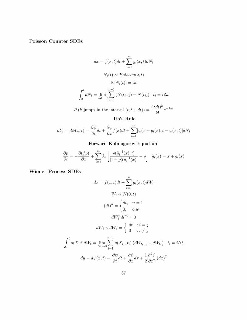
Poisson Counter SDEs
dx = f(x, t)dt+
m∑i=1
gi(x, t)dNi
Ni(t) ∼ Poisson(λit)
E [Ni(t)] = λt
t
0dNt = lim
∆t→0
n−1∑i=0
(N(ti+1)−N(ti)) ti = i∆t
P (k jumps in the interval (t, t+ dt)) =(λdt)k
k!e−λdt
Ito’s Rule
dYt = dψ(x, t) =∂ψ
∂tdt+
∂ψ
∂xf(x)dt+
m∑i=1
[ψ(x+ gi(x), t− ψ(x, t)]dNi
Forward Kolmogorov Equation
∂p
∂t= −∂(fp)
∂x+
m∑i=1
λi
[ρ(g−1
i (x), t)
|1 + g′i(g−1i (x)|
− ρ]
gi(x) = x+ gi(x)
Wiener Process SDEs
dx = f(x, t)dt+n∑i=1
gi(x, t)dWi
Wt ∼ N(0, t)
(dt)n =
dt, n = 1
0, o.w
dWni dt
m = 0
dWi × dWj =
dt : i = j0 : i 6= j
t
0g(X, t)dWt = lim
∆t→0
n−1∑i=1
g(Xti , ti)(dWti+1 − dWti
)ti = i∆t
dy = dψ(x, t) =∂ψ
∂tdt+
∂ψ
∂xdx+
1
2
∂2ψ
∂x2(dx)2
87
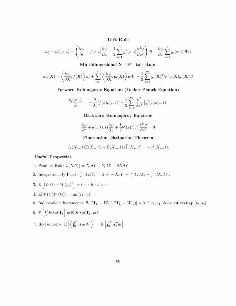
Ito’s Rule
dy = dψ(x, t) =
(∂ψ
∂t+ f(x, t)
∂ψ
∂x+
1
2
n∑i=1
g2i (x, t)
∂2ψ
∂x2
)dt+
∂ψ
∂x
n∑i=1
gi(x, t)dWi
Multidimensional X ∈ Rn Ito’s Rule
dψ(X) =
⟨∂ψ
∂X, f(X)
⟩dt+
m∑i=1
⟨∂ψ
∂X, gi(X)
⟩dWi +
1
2
m∑i=1
gi(X)T∇2ψ(X)gi(X)dt
Forward Kolmogorov Equation (Fokker-Planck Equation)
∂ρ(x, t)
∂t= − ∂
∂x[f(x)ρ(x, t)] +
1
2
m∑i=1
∂2
∂x2
[g2i (x)ρ(x, t)
]Backward Kolmogorov Equation
∂ρ
∂t+ a(x(t), t)
∂ρ
∂x+
1
2b2(x(t), t)
∂2ρ
∂x2= 0
Fluctuation-Dissipation Theorem
Jf (Xss, t)Σ(Xss, t) + Σ(Xss, t)JTf (Xss, t) = −g2(Xss, t).
Useful Properties
1. Product Rule: d(XtYt) = XtdY + YtdX + dXdY .
2. Integration By Parts: t
0 XtdYt = XtYt −X0Y0 − t
0 YtdXt − t
0 dXtdYt.
3. E[(W (t)−W (s))2
]= t− s for t > s.
4. E[W (t1)W (t2)] = min(t1, t2).
5. Independent Increments: E [(Wti −Ws1) (Wt2 −Ws2)] = 0 if [t1, s1] does not overlap [t2, s2].
6. E[ t
0 h(t)dWt
]= E [h(t)dWt] = 0.
7. Ito Isometry: E[( T
0 XtdWt
)]= E
[ T0 X2
t dt]
88
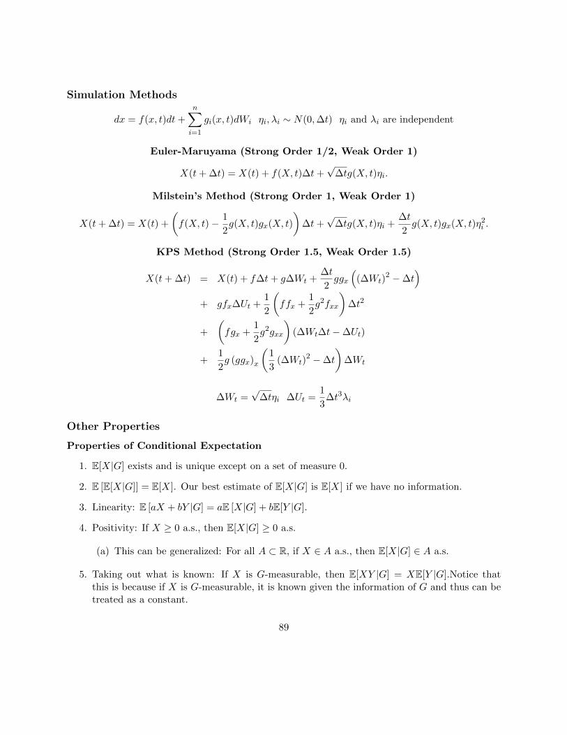
Simulation Methods
dx = f(x, t)dt+n∑i=1
gi(x, t)dWi ηi, λi ∼ N(0,∆t) ηi and λi are independent
Euler-Maruyama (Strong Order 1/2, Weak Order 1)
X(t+ ∆t) = X(t) + f(X, t)∆t+√
∆tg(X, t)ηi.
Milstein’s Method (Strong Order 1, Weak Order 1)
X(t+ ∆t) = X(t) +
(f(X, t)− 1
2g(X, t)gx(X, t)
)∆t+
√∆tg(X, t)ηi +
∆t
2g(X, t)gx(X, t)η2
i .
KPS Method (Strong Order 1.5, Weak Order 1.5)
X(t+ ∆t) = X(t) + f∆t+ g∆Wt +∆t
2ggx
((∆Wt)
2 −∆t)
+ gfx∆Ut +1
2
(ffx +
1
2g2fxx
)∆t2
+
(fgx +
1
2g2gxx
)(∆Wt∆t−∆Ut)
+1
2g (ggx)x
(1
3(∆Wt)
2 −∆t
)∆Wt
∆Wt =√
∆tηi ∆Ut =1
3∆t3λi
Other Properties
Properties of Conditional Expectation
1. E[X|G] exists and is unique except on a set of measure 0.
2. E [E[X|G]] = E[X]. Our best estimate of E[X|G] is E[X] if we have no information.
3. Linearity: E [aX + bY |G] = aE [X|G] + bE[Y |G].
4. Positivity: If X ≥ 0 a.s., then E[X|G] ≥ 0 a.s.
(a) This can be generalized: For all A ⊂ R, if X ∈ A a.s., then E[X|G] ∈ A a.s.
5. Taking out what is known: If X is G-measurable, then E[XY |G] = XE[Y |G].Notice thatthis is because if X is G-measurable, it is known given the information of G and thus can betreated as a constant.
89
6. Iterated Conditioning: If H ⊂ G ⊂ F , then E [E[X|G]|H] = E[X|H].
7. Independence of G: If X is independent of G, then E[X|G] = E[X]. If G gives no informationabout X, then the expectation condition on the information of G is simply the expectationof X.
8. If Mt is a martingale, then E[Mt|Fs] = Ms.
90