Publication 97/2

An Introduction to TurbulenceModels

Lars Davidson, http://www.tfd.chalmers.se/˜lada

Department of Thermo and Fluid DynamicsCHALMERS UNIVERSITY OF TECHNOLOGY

Goteborg, Sweden, September 14, 2017

CONTENTS 2

Contents

Nomenclature 3

1 Turbulence 5

1.1 Introduction . . . . . . . . . . . . . . . . . . . . . . . . . . . . 51.2 Turbulent Scales . . . . . . . . . . . . . . . . . . . . . . . . . . 61.3 Vorticity/Velocity Gradient Interaction . . . . . . . . . . . . . 71.4 Energy spectrum . . . . . . . . . . . . . . . . . . . . . . . . . 9

2 Turbulence Models 12

2.1 Introduction . . . . . . . . . . . . . . . . . . . . . . . . . . . . 122.2 Boussinesq Assumption . . . . . . . . . . . . . . . . . . . . . 152.3 Algebraic Models . . . . . . . . . . . . . . . . . . . . . . . . . 162.4 Equations for Kinetic Energy . . . . . . . . . . . . . . . . . . 16

2.4.1 The Exact k Equation . . . . . . . . . . . . . . . . . . . 162.4.2 The Equation for 1/2(UiUi) . . . . . . . . . . . . . . . 18

2.5 The Modelled k Equation . . . . . . . . . . . . . . . . . . . . 202.6 One Equation Models . . . . . . . . . . . . . . . . . . . . . . . 21

3 Two-Equation Turbulence Models 22

3.1 The Modelled ε Equation . . . . . . . . . . . . . . . . . . . . . 223.2 Wall Functions . . . . . . . . . . . . . . . . . . . . . . . . . . . 223.3 The k − ε Model . . . . . . . . . . . . . . . . . . . . . . . . . . 253.4 The k − ω Model . . . . . . . . . . . . . . . . . . . . . . . . . 263.5 The k − τ Model . . . . . . . . . . . . . . . . . . . . . . . . . . 27

4 Low-Re Number Turbulence Models 28

4.1 Low-Re k − ε Models . . . . . . . . . . . . . . . . . . . . . . . 294.2 The Launder-Sharma Low-Re k − ε Models . . . . . . . . . . 324.3 Boundary Condition for ε and ε . . . . . . . . . . . . . . . . . 334.4 The Two-Layer k − ε Model . . . . . . . . . . . . . . . . . . . 344.5 The low-Re k − ω Model . . . . . . . . . . . . . . . . . . . . . 35

4.5.1 The low-Re k − ω Model of Peng et al. . . . . . . . . . 364.5.2 The low-Re k − ω Model of Bredberg et al. . . . . . . . 36

5 Reynolds Stress Models 38

5.1 Reynolds Stress Models . . . . . . . . . . . . . . . . . . . . . 395.2 Reynolds Stress Models vs. Eddy Viscosity Models . . . . . . 405.3 Curvature Effects . . . . . . . . . . . . . . . . . . . . . . . . . 415.4 Acceleration and Retardation . . . . . . . . . . . . . . . . . . 44

2

Nomenclature 3

Nomenclature

Latin Symbols

c1, c2, cs constants in the Reynolds stress modelc′1, c

′2 constants in the Reynolds stress model

cε1, cε2 constants in the modelled ε equationcω1, cω2 constants in the modelled ω equationcµ constant in turbulence modelE energy (see Eq. 1.8); constant in wall functions (see Eq. 3.4)f damping function in pressure strain tensork turbulent kinetic energy (≡ 1

2uiui)

U instantaneous (or laminar) velocity in x-directionUi instantaneous (or laminar) velocity in xi-directionU time-averaged velocity in x-directionUi time-averaged velocity in xi-directionuv, uw shear stressesu fluctuating velocity in x-direction

u2 normal stress in the x-directionui fluctuating velocity in xi-directionuiuj Reynolds stress tensorV instantaneous (or laminar) velocity in y-directionV time-averaged velocity in y-directionv fluctuating (or laminar) velocity in y-direction

v2 normal stress in the y-directionvw shear stressW instantaneous (or laminar) velocity in z-directionW time-averaged velocity in z-directionw fluctuating velocity in z-direction

w2 normal stress in the z-direction

Greek Symbols

δ boundary layer thickness; half channel heightε dissipationκ wave number; von Karman constant (= 0.41)µ dynamic viscosityµt dynamic turbulent viscosityν kinematic viscosityνt kinematic turbulent viscosityΩi instantaneous (or laminar) vorticity component in xi-direction

3

Nomenclature 4

Ωi time-averaged vorticity component in xi-directionω specific dissipation (∝ ε/k)ωi fluctuating vorticity component in xi-directionσΦ turbulent Prandtl number for variable Φτlam laminar shear stressτtot total shear stressτturb turbulent shear stress

Subscript

C centerlinew wall

4

5

1 Turbulence

1.1 Introduction

Almost all fluid flow which we encounter in daily life is turbulent. Typicalexamples are flow around (as well as in) cars, aeroplanes and buildings.The boundary layers and the wakes around and after bluff bodies such ascars, aeroplanes and buildings are turbulent. Also the flow and combustionin engines, both in piston engines and gas turbines and combustors, arehighly turbulent. Air movements in rooms are also turbulent, at least alongthe walls where wall-jets are formed. Hence, when we compute fluid flowit will most likely be turbulent.

In turbulent flow we usually divide the variables in one time-averagedpart U , which is independent of time (when the mean flow is steady), andone fluctuating part u so that U = U + u.

There is no definition on turbulent flow, but it has a number of charac-teristic features (see Tennekes & Lumley [44]) such as:

I. Irregularity. Turbulent flow is irregular, random and chaotic. Theflow consists of a spectrum of different scales (eddy sizes) where largesteddies are of the order of the flow geometry (i.e. boundary layer thickness,jet width, etc). At the other end of the spectra we have the smallest ed-dies which are by viscous forces (stresses) dissipated into internal energy.Even though turbulence is chaotic it is deterministic and is described bythe Navier-Stokes equations.

II. Diffusivity. In turbulent flow the diffusivity increases. This meansthat the spreading rate of boundary layers, jets, etc. increases as the flowbecomes turbulent. The turbulence increases the exchange of momentumin e.g. boundary layers and reduces or delays thereby separation at bluffbodies such as cylinders, airfoils and cars. The increased diffusivity alsoincreases the resistance (wall friction) in internal flows such as in channelsand pipes.

III. Large Reynolds Numbers. Turbulent flow occurs at high Reynoldsnumber. For example, the transition to turbulent flow in pipes occurs thatReD ≃ 2300, and in boundary layers at Rex ≃ 100000.

IV. Three-Dimensional. Turbulent flow is always three-dimensional.However, when the equations are time averaged we can treat the flow astwo-dimensional.

V. Dissipation. Turbulent flow is dissipative, which means that ki-netic energy in the small (dissipative) eddies are transformed into internalenergy. The small eddies receive the kinetic energy from slightly larger ed-dies. The slightly larger eddies receive their energy from even larger eddiesand so on. The largest eddies extract their energy from the mean flow. Thisprocess of transferred energy from the largest turbulent scales (eddies) tothe smallest is called cascade process.

5

1.2 Turbulent Scales 6

VI. Continuum. Even though we have small turbulent scales in theflow they are much larger than the molecular scale and we can treat theflow as a continuum.

1.2 Turbulent Scales

As mentioned above there are a wide range of scales in turbulent flow (youcan read more about turbulence in [14]). The larger scales are of the order ofthe flow geometry, for example the boundary layer thickness, with lengthscale ℓ and velocity scale U . These scales extract kinetic energy from themean flow which has a time scale comparable to the large scales, i.e.

∂U

∂y= O(T −1) = O(U/ℓ)

The kinetic energy of the large scales is lost to slightly smaller scales withwhich the large scales interact. Through the cascade process the kinetic en-ergy is in this way transferred from the largest scale to smaller scales. Atthe smallest scales the frictional forces (viscous stresses) become too largeand the kinetic energy is transformed (dissipated) into internal energy. Thedissipation is denoted by ε which is energy per unit time and unit mass(ε = [m2/s3]). The dissipation is proportional to the kinematic viscosity νtimes the fluctuating velocity gradient up to the power of two (see Sec-tion 2.4.1). The friction forces exist of course at all scales, but they arelarger the smaller the eddies. Thus it is not quite true that eddies whichreceive their kinetic energy from slightly larger scales give away all of thatthe slightly smaller scales but a small fraction is dissipated. However it isassumed that most of the energy (say 90 %) that goes into the large scalesis finally dissipated at the smallest (dissipative) scales.

The smallest scales where dissipation occurs are called the Kolmogo-rov scales: the velocity scale υ, the length scale η and the time scale τ . Weassume that these scales are determined by viscosity ν and dissipation ε.Since the kinetic energy is destroyed by viscous forces it is natural to as-sume that viscosity plays a part in determining these scales; the larger vis-cosity, the larger scales. The amount of energy that is to be dissipated isε. The more energy that is to be transformed from kinetic energy to inter-nal energy, the larger the velocity gradients must be. Having assumed thatthe dissipative scales are determined by viscosity and dissipation, we canexpress υ, η and τ in ν and ε using dimensional analysis. We write

υ = νa εb

[m/s] = [m2/s] [m2/s3](1.1)

where below each variable its dimensions are given. The dimensions of theleft-hand and the right-hand side must be the same. We get two equations,

6

1.3 Vorticity/Velocity Gradient Interaction 7

one for meters [m]

1 = 2a+ 2b, (1.2)

and one for seconds [s]

−1 = −a− 3b, (1.3)

which gives a = b = 1/4. In the same way we obtain the expressions for ηand τ so that

υ = (νε)1/4 , η =

(ν3

ε

)1/4

, τ =(ν

ε

)1/2(1.4)

1.3 Vorticity/Velocity Gradient Interaction

The interaction between vorticity and velocity gradients is an essential in-gredient to create and maintain turbulence. Disturbances are amplified– the actual process depending on type of flow – and these disturbances,which still are laminar and organized and well defined in terms of phys-ical orientation and frequency are turned into chaotic, three-dimensional,random fluctuations, i.e. turbulent flow by interaction between the vor-ticity vector and the velocity gradients. Two idealized phenomena in thisinteraction process can be identified: vortex stretching and vortex tilting.

In order to gain some insight in vortex shedding we will study an ide-alized, inviscid (viscosity equals to zero) case. The equation for instanta-neous vorticity (Ωi = Ωi + ωi) reads [44, 34, 47]

UjΩi,j = ΩjUi,j + νΩi,jj

Ωi = ǫijkUk,j

(1.5)

where ǫijk is the Levi-Civita tensor (it is +1 if i, j k are in cyclic order, −1 ifi, j k are in anti-cyclic order, and 0 if any two of i, j k are equal), and where(.),j denotes derivation with respect to xj . We see that this equation is notan ordinary convection-diffusion equation but is has an additional term onthe right-hand side which represents amplification and rotation/tilting ofthe vorticity lines. If we write it term-by-term it reads

Ω1U1,1 +Ω2U1,2 +Ω3U1,3 (1.6)

Ω1U2,1 +Ω2U2,2 +Ω3U2,3

Ω1U3,1 +Ω2U3,2 +Ω3U3,3

The diagonal terms in this matrix represent vortex stretching. Imagine a Vortexstretchingslender, cylindrical fluid element which vorticity Ω. We introduce a cylin-

drical coordinate system with the x1-axis as the cylinder axis and x2 as the

7

1.3 Vorticity/Velocity Gradient Interaction 8

Ω1 Ω1

Figure 1.1: Vortex stretching.

radial coordinate (see Fig. 1.1) so that Ω = (Ω1, 0, 0). A positive U1,1 willstretch the cylinder. From the continuity equation

U1,1 +1

r(rU2),2 = 0

we find that the radial derivative of the radial velocity U2 must be negative,i.e. the radius of the cylinder will decrease. We have neglected the viscositysince viscous diffusion at high Reynolds number is much smaller than theturbulent one and since viscous dissipation occurs at small scales (see p. 6).Thus there are no viscous stresses acting on the cylindrical fluid elementsurface which means that the rotation momentum

r2Ω (1.7)

remains constant as the radius of the fluid element decreases (note that alsothe circulation Γ ∝ Ωr2 is constant). Equation 1.7 shows that the vortic-ity increases as the radius decreases. We see that a stretching/compressingwill decrease/increase the radius of a slender fluid element and increase/decreaseits vorticity component aligned with the element. This process will affectthe vorticity components in the other two coordinate directions.

The off-diagonal terms in Eq. 1.6 represent vortex tilting. Again, take a Vortextiltingslender fluid element with its axis aligned with the x2 axis, Fig. 1.2. The ve-

locity gradient U1,2 will tilt the fluid element so that it rotates in clock-wisedirection. The second term Ω2U1,2 in line one in Eq. 1.6 gives a contributionto Ω1.

Vortex stretching and vortex tilting thus qualitatively explains how in-teraction between vorticity and velocity gradient create vorticity in all threecoordinate directions from a disturbance which initially was well definedin one coordinate direction. Once this process has started it continues, be-cause vorticity generated by vortex stretching and vortex tilting interactswith the velocity field and creates further vorticity and so on. The vortic-ity and velocity field becomes chaotic and random: turbulence has beencreated. The turbulence is also maintained by these processes.

From the discussion above we can now understand why turbulence al-ways must be three-dimensional (Item IV on p. 5). If the instantaneousflow is two-dimensional we find that all interaction terms between vortic-ity and velocity gradients in Eq. 1.6 vanish. For example if U3 ≡ 0 and allderivatives with respect to x3 are zero. If U3 ≡ 0 the third line in Eq. 1.6vanishes, and if Ui,3 ≡ 0 the third column in Eq. 1.6 disappears. Finally, the

8

1.4 Energy spectrum 9

Ω2

Ω2

U1(x2)

Figure 1.2: Vortex tilting.

remaining terms in Eq. 1.6 will also be zero since

Ω1 = U3,2 − U2,3 ≡ 0

Ω2 = U1,3 − U3,1 ≡ 0.

The interaction between vorticity and velocity gradients will, on av-erage, create smaller and smaller scales. Whereas the large scales whichinteract with the mean flow have an orientation imposed by the mean flowthe small scales will not remember the structure and orientation of the largescales. Thus the small scales will be isotropic, i.e independent of direction.

1.4 Energy spectrum

The turbulent scales are distributed over a range of scales which extendsfrom the largest scales which interact with the mean flow to the smallestscales where dissipation occurs. In wave number space the energy of ed-dies from κ to κ+ dκ can be expressed as

E(κ)dκ (1.8)

where Eq. 1.8 expresses the contribution from the scales with wave numberbetween κ and κ + dκ to the turbulent kinetic energy k. The dimensionof wave number is one over length; thus we can think of wave numberas proportional to the inverse of an eddy’s radius, i.e κ ∝ 1/r. The totalturbulent kinetic energy is obtained by integrating over the whole wavenumber space i.e.

k =

∫ ∞

0

E(κ)dκ (1.9)

9

1.4 Energy spectrum 10

I

II

III

κ

E(κ)

Figure 1.3: Spectrum for k. I: Range for the large, energy containing eddies.II: the inertial subrange. III: Range for small, isotropic scales.

The kinetic energy is the sum of the kinetic energy of the three fluctuat-ing velocity components, i.e.

k =1

2

(

u2 + v2 + w2

)

=1

2uiui (1.10)

The spectrum of E is shown in Fig. 1.3. We find region I, II and III whichcorrespond to:

I. In the region we have the large eddies which carry most of the energy.These eddies interact with the mean flow and extract energy from themean flow. Their energy is past on to slightly smaller scales. Theeddies’ velocity and length scales are U and ℓ, respectively.

III. Dissipation range. The eddies are small and isotropic and it is herethat the dissipation occurs. The scales of the eddies are described bythe Kolmogorov scales (see Eq. 1.4)

II. Inertial subrange. The existence of this region requires that the Reynoldsnumber is high (fully turbulent flow). The eddies in this region repre-sent the mid-region. This region is a “transport” region in the cascadeprocess. Energy per time unit (ε) is coming from the large eddies atthe lower part of this range and is given off to the dissipation rangeat the higher part. The eddies in this region are independent of boththe large, energy containing eddies and the eddies in the dissipationrange. One can argue that the eddies in this region should be char-acterized by the flow of energy (ε) and the size of the eddies 1/κ.Dimensional reasoning gives

E(κ) = const. ε2

3κ−5

3 (1.11)

This is a very important law (Kolmogorov spectrum law or the −5/3law) which states that, if the flow is fully turbulent (high Reynolds

10

1.4 Energy spectrum 11

number), the energy spectra should exhibit a −5/3-decay. This of-ten used in experiment and Large Eddy Simulations (LES) and DirectNumerical Simulations (DNS) to verify that the flow is fully turbu-lent.

As explained on p. 6 (cascade process) the energy dissipated at the smallscales can be estimated using the large scales U and ℓ. The energy at thelarge scales lose their energy during a time proportional to ℓ/U , which gives

ε = O( U2

ℓ/U

)

= O(U3

ℓ

)

(1.12)

11

12

2 Turbulence Models

2.1 Introduction

You can read more about turbulence models in[14].When the flow is turbulent it is preferable to decompose the instan-

taneous variables (for example velocity components and pressure) into amean value and a fluctuating value, i.e.

Ui = Ui + ui

P = P + p.(2.1)

One reason why we decompose the variables is that when we measure flowquantities we are usually interested in the mean values rather that the timehistories. Another reason is that when we want to solve the Navier-Stokesequation numerically it would require a very fine grid to resolve all tur-bulent scales and it would also require a fine resolution in time (turbulentflow is always unsteady).

The continuity equation and the Navier-Stokes equation read

∂ρ

∂t+ (ρUi),i = 0 (2.2)

∂ρUi

∂t+ (ρUiUj),j = −P,i +

[

µ

(

Ui,j + Uj,i −2

3δijUk,k

)]

,j

(2.3)

where (.),j denotes derivation with respect to xj . Since we are dealing withincompressible flow (i.e low Mach number) the dilatation term on the right-hand side of Eq. 2.3 is neglected so that

∂ρUi

∂t+ (ρUiUj),j = −P,i + [µ(Ui,j + Uj,i)],j . (2.4)

Note that we here use the term “incompressible” in the sense that density isindependent of pressure (∂P/∂ρ = 0) , but it does not mean that density isconstant; it can be dependent on for example temperature or concentration.

Inserting Eq. 2.1 into the continuity equation (2.2) and the Navier-Stokesequation (2.4) and we obtain – after time averaging – the time averaged con-tinuity equation and Navier-Stokes equation

∂ρ

∂t+ (ρUi),i = 0 (2.5)

∂ρUi

∂t+(ρUiUj

)

,j= −P,i +

[µ(Ui,j + Uj,i)− ρuiuj

]

,j. (2.6)

A new term uiuj appears on the right-hand side of Eq. 2.6 which iscalled the Reynolds stress tensor. The tensor is symmetric (for example u1u2 =u2u1). It represents correlations between fluctuating velocities. It is an ad-ditional stress term due to turbulence (fluctuating velocities) and it is un-known. We need a model for uiuj to close the equation system in Eq. 2.6.

12

2.1 Introduction 13

y

τ

τlam

τturbτtot

y+ ≃ 10Figure 2.1: Shear stress near a wall.

This is called the closure problem: the number of unknowns (ten: three veloc- closureproblemity components, pressure, six stresses) is larger than the number of equa-

tions (four: the continuity equation and three components of the Navier-Stokes equations).

For steady, two-dimensional boundary-layer type of flow (i.e. bound-ary layers along a flat plate, channel flow, pipe flow, jet and wake flow, etc.)where

V ≪ U ,∂

∂x≪ ∂

∂y(2.7)

Eq. 2.6 reads

∂ρUU

∂x+

∂ρV U

∂y= −∂P

∂x+

∂

∂y

[

µ∂U

∂y− ρuv

]

︸ ︷︷ ︸

τtot

. (2.8)

x = x1 denotes streamwise coordinate, and y = x2 coordinate normal tothe flow. Often the pressure gradient ∂P /∂x is zero.

To the viscous shear stress µ∂U/∂y on the right-hand side of Eq. 2.8 shearstressappears an additional turbulent one, a turbulent shear stress. The total shear

stress is thus

τtot = µ∂U

∂y− ρuv

In the wall region (the viscous sublayer, the buffert layer and the logarith-mic layer) the total shear stress is approximately constant and equal to thewall shear stress τw, see Fig. 2.1. Note that the total shear stress is constantonly close to the wall; further away from the wall it decreases (in fully de-veloped channel flow it decreases linearly by the distance form the wall).At the wall the turbulent shear stress vanishes as u = v = 0, and the viscousshear stress attains its wall-stress value τw = ρu2∗. As we go away from thewall the viscous stress decreases and turbulent one increases and at y+ ≃ 10they are approximately equal. In the logarithmic layer the viscous stress isnegligible compared to the turbulent stress.

In boundary-layer type of flow the turbulent shear stress and the ve-locity gradient ∂U/∂y have nearly always opposite sign (for a wall jet this

13

2.1 Introduction 14

x

y

v < 0 v > 0

y1

y2

U(y)

Figure 2.2: Sign of the turbulent shear stress −ρuv in a boundary layer.

is not the case close to the wall). To get a physical picture of this let usstudy the flow in a boundary layer, see Fig. 2.2. A fluid particle is movingdownwards (particle drawn with solid line) from y2 to y1 with (the turbu-lent fluctuating) velocity v. At its new location the U velocity is in averagesmaller than at its old, i.e. U(y1) < U(y2). This means that when the par-ticle at y2 (which has streamwise velocity U(y2)) comes down to y1 (wherethe streamwise velocity is U(y1)) is has an excess of streamwise velocitycompared to its new environment at y1. Thus the streamwise fluctuation ispositive, i.e. u > 0 and the correlation between u and v is negative (uv < 0).

If we look at the other particle (dashed line in Fig. 2.2) we reach thesame conclusion. The particle is moving upwards (v > 0), and it is bringinga deficit in U so that u < 0. Thus, again, uv < 0. If we study this flow fora long time and average over time we get uv < 0. If we change the signof the velocity gradient so that ∂U/∂y < 0 we will find that the sign of uvalso changes.

Above we have used physical reasoning to show the the signs of uvand ∂U/∂y are opposite. This can also be found by looking at the produc-tion term in the transport equation of the Reynolds stresses (see Section 5).In cases where the shear stress and the velocity gradient have the samesign (for example, in a wall jet) this means that there are other terms in thetransport equation which are more important than the production term.

There are different levels of approximations involved when closing theequation system in Eq. 2.6.

I. Algebraic models. An algebraic equation is used to compute a tur-bulent viscosity, often called eddy viscosity. The Reynolds stress ten-sor is then computed using an assumption which relates the Reynoldsstress tensor to the velocity gradients and the turbulent viscosity. Thisassumption is called the Boussinesq assumption. Models which arebased on a turbulent (eddy) viscosity are called eddy viscosity mod-

14

2.2 Boussinesq Assumption 15

els.

II. One-equation models. In these models a transport equation is solvedfor a turbulent quantity (usually the turbulent kinetic energy) anda second turbulent quantity (usually a turbulent length scale) is ob-tained from an algebraic expression. The turbulent viscosity is calcu-lated from Boussinesq assumption.

III. Two-equation models. These models fall into the class of eddy vis-cosity models. Two transport equations are derived which describetransport of two scalars, for example the turbulent kinetic energy kand its dissipation ε. The Reynolds stress tensor is then computedusing an assumption which relates the Reynolds stress tensor to thevelocity gradients and an eddy viscosity. The latter is obtained fromthe two transported scalars.

IV. Reynolds stress models. Here a transport equation is derived forthe Reynolds tensor uiuj . One transport equation has to be added fordetermining the length scale of the turbulence. Usually an equationfor the dissipation ε is used.

Above the different types of turbulence models have been listed in in-creasing order of complexity, ability to model the turbulence, and cost interms of computational work (CPU time).

2.2 Boussinesq Assumption

In eddy viscosity turbulence models the Reynolds stresses are linked tothe velocity gradients via the turbulent viscosity: this relation is called theBoussinesq assumption, where the Reynolds stress tensor in the time aver-aged Navier-Stokes equation is replaced by the turbulent viscosity multi-plied by the velocity gradients. To show this we introduce this assumptionfor the diffusion term at the right-hand side of Eq. 2.6 and make an identi-fication

[µ(Ui,j + Uj,i)− ρuiuj

]

,j=[(µ+ µt)(Ui,j + Uj,i)

]

,j

which gives

ρuiuj = −µt(Ui,j + Uj,i). (2.9)

If we in Eq. 2.9 do a contraction (i.e. setting indices i = j) the right-handside gives

uiui ≡ 2k

where k is the turbulent kinetic energy (see Eq. 1.10). On the other handthe continuity equation (Eq. 2.5) gives that the right-hand side of Eq. 2.9

15

2.3 Algebraic Models 16

is equal to zero. In order to make Eq. 2.9 valid upon contraction we add2/3ρδijk to the left-hand side of Eq. 2.9 so that

ρuiuj = −µt(Ui,j + Uj,i) +2

3δijρk. (2.10)

Note that contraction of δij gives

δii = δ11 + δ22 + δ33 = 1 + 1 + 1 = 3

2.3 Algebraic Models

In eddy viscosity models we want an expression for the turbulent viscosityµt = ρνt. The dimension of νt is [m2/s] (same as ν). A turbulent velocity Eddy

viscositymodel

scale multiplied with a turbulent length scale gives the correct dimension,i.e.

νt ∝ Uℓ (2.11)

Above we have used U and ℓ which are characteristic for the large turbulentscales. This is reasonable, because it is these scales which are responsiblefor most of the transport by turbulent diffusion.

In an algebraic turbulence model the velocity gradient is used as a ve-locity scale and some physical length is used as the length scale. In bound-ary layer-type of flow (see Eq. 2.7) we obtain

νt = ℓ2mix

∣∣∣∣

∂U

∂y

∣∣∣∣

(2.12)

where y is the coordinate normal to the wall, and where ℓmix is the mixinglength, and the model is called the mixing length model. It is an old modeland is hardly used any more. One problem with the model is that ℓmix isunknown and must be determined.

More modern algebraic models are the Baldwin-Lomax model [2] andthe Cebeci-Smith [6] model which are frequently used in aerodynamicswhen computing the flow around airfoils, aeroplanes, etc. For a presen-tation and discussion of algebraic turbulence models the interested readeris referred to Wilcox [49].

2.4 Equations for Kinetic Energy

2.4.1 The Exact k Equation

The equation for turbulent kinetic energy k = 1

2uiui is derived from the

Navier-Stokes equation which reads assuming steady, incompressible, con-stant viscosity (cf. Eq. 2.4)

(ρUiUj),j = −P,i + µUi,jj. (2.13)

16

2.4 Equations for Kinetic Energy 17

The time averaged Navier-Stokes equation reads (cf. Eq. 2.6)

(ρUiUj),j = −P,i + µUi,jj − ρ(uiuj),j (2.14)

Subtract Eq. 2.14 from Eq. 2.13, multiply by ui and time average and weobtain

[ρUiUj − ρUiUj

]

,jui =

−[P − P

]

,iui + µ

[Ui − Ui

]

,jjui + ρ(uiuj),jui

(2.15)

The left-hand side can be rewritten as

ρ[(Ui + ui)(Uj + uj)− UiUj

]

,jui = ρ

[Uiuj + uiUj + uiuj

]

,jui. (2.16)

Using the continuity equation (ρuj),j = 0, the first term is rewritten as(ρUiuj

)

,jui = ρuiujUi,j. (2.17)

We obtain the second term (using (ρUj),j = 0) from

(ρUjk

)

,j= Ujρ

[1

2uiui

]

,j

=

1

2ρUj uiui,j + uiui,j = ui

(ρUjui

)

,j

(2.18)

The third term in Eq. 2.16 can be written as (using the same technique as inEq. 2.18)

1

2(ρujuiui),j. (2.19)

The first term on the right-hand side of Eq. 2.15 has the form

−p,iui = −(pui),i (2.20)

The second term on the right-hand side of Eq. 2.15 reads

µui,jjui = µ

(ui,jui),j − ui,jui,j

(2.21)

For the first term we use the same trick as in Eq. 2.18 so that

µ(ui,jui),j = µ1

2(uiui),jj = µk,jj (2.22)

The last term on the right-hand side of Eq. 2.15 is zero. Now we canassemble the transport equation for the turbulent kinetic energy. Equa-tions 2.17, 2.18, 2.20, 2.21,2.22 give

(ρUjk),j︸ ︷︷ ︸

I

= −ρuiujUi,j︸ ︷︷ ︸

II

−[

ujp+1

2ρujuiui − µk,j

]

,j︸ ︷︷ ︸

III

−µui,jui,j︸ ︷︷ ︸

IV

(2.23)

The terms in Eq. 2.23 have the following meaning.

17

2.4 Equations for Kinetic Energy 18

0 5 10 15 200

0.05

0.1

0.15

0.2

0.25

x+2Figure 2.3: Channel flow at Reτ = 2000. Comparison of mean and fluc-tuating dissipation terms. Both terms are normalized by u4τ/ν. DNSdata [22, 21]. Solid line: ν(∂V1/∂x2)

2; dashed line: ε.

I. Convection.

II. Production. The large turbulent scales extract energy from the meanflow. This term (including the minus sign) is almost always positive.

III. The two first terms represent turbulent diffusion by pressure-velocityfluctuations, and velocity fluctuations, respectively. The last term isviscous diffusion.

IV. Dissipation. This term is responsible for transformation of kineticenergy at small scales to internal energy. The term (including theminus sign) is always negative.

In boundary-layer flow the exact k equation read

∂ρUk

∂x+

∂ρV k

∂y= −ρuv

∂U

∂y− ∂

∂y

[

pv +1

2ρvuiui − µ

∂k

∂y

]

− µui,jui,j(2.24)

Note that the dissipation includes all derivatives. This is because the dis-sipation term is at its largest for small, isotropic scales where the usualboundary-layer approximation that ∂ui/∂x ≪ ∂ui/∂y is not valid.

2.4.2 The Equation for 1/2(UiUi)

The equation for 1/2(UiUi) is derived in the same way as that for 1/2u′iu′i.

Assume steady, incompressible flow with constant viscosity and multiplythe time-averaged Navier-Stokes equations (Eq. 2.14) so that

Ui(ρUiUj),j = −UiP,i + µUiUi,jj − Uiρ(uiuj),j. (2.25)

The term on the left-hand side can be rewritten as

(ρUiUiUj),j − ρUiUjUi,j = ρUj(UiUi),j −1

2ρUj(UiUi),j

=1

2ρUj(UiUi),j = (ρUjKK),j

(2.26)

18

2.5 The Modelled k Equation 19

The first term on the right-hand side of Eq. 2.25 can be written as

−UiP,i = −(UiP ),i. (2.27)

The viscous term in Eq. 2.25 is rewritten in the same way as the viscousterm in Section 2.4.1, see Eqs. 2.21 and 2.22, i.e.

µUiUi,jj = µK,jj − µUi,jUi,j. (2.28)

Now we can assemble the transport equation for K by inserting Eqs. 2.26,2.27 and 2.28 into Eq. 2.25

(ρUjK),j = µK,jj − (UiP ),i − µUi,jUi,j − Uiρ(uiuj),j, (2.29)

where K = 1/2(UiUi). The last term is rewritten as

−Uiρ(uiuj),j = −(Uiρuiuj),j + ρ(uiuj)Ui,j. (2.30)

Inserted in Eq. 2.29 gives

(ρUjK),j = µK,jj − (UiP ),i − µUi,jUi,j

− (Uiρuiuj),j + ρuiujUi,j .(2.31)

On the left-hand side we have the usual convective term. On the right-handside we find: transport by viscous diffusion, transport by pressure-velocityinteraction, viscous dissipation, transport by velocity-stress interaction andloss of energy to the fluctuating velocity field, i.e. to k. Note that the lastterm in Eq. 2.31 is the same as the last term in Eq. 2.23 but with oppositesign: here we clearly can see that the main source term in the k equation(the production term) appears as a sink term in the K equation.

In the K equation the dissipation term and the negative productionterm (representing loss of kinetic energy to the k field) read

−µUi,jUi,j + ρuiujUi,j, (2.32)

and in the k equation the production and the dissipation terms read

−ρuiujUi,j − µui,jui,j. (2.33)

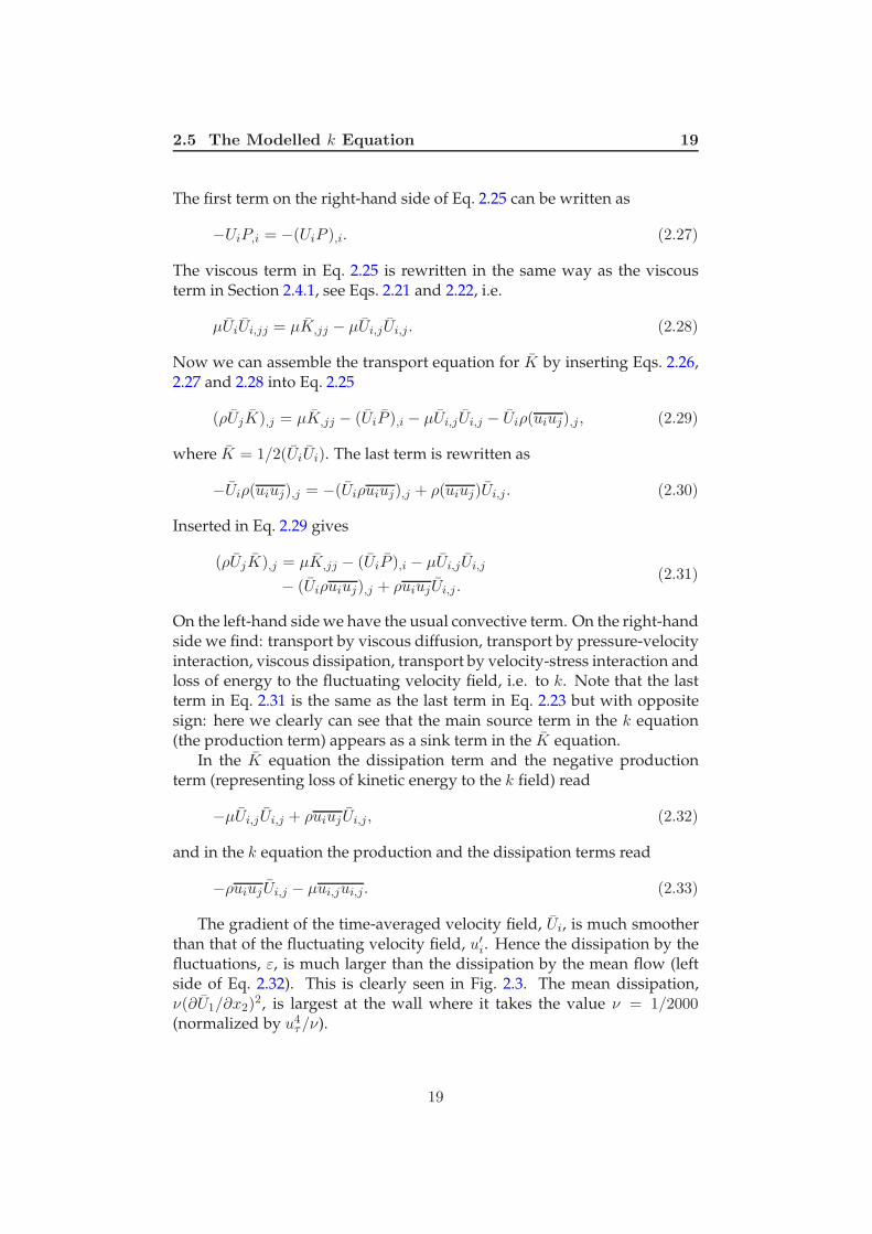
The gradient of the time-averaged velocity field, Ui, is much smootherthan that of the fluctuating velocity field, u′i. Hence the dissipation by thefluctuations, ε, is much larger than the dissipation by the mean flow (leftside of Eq. 2.32). This is clearly seen in Fig. 2.3. The mean dissipation,ν(∂U1/∂x2)

2, is largest at the wall where it takes the value ν = 1/2000(normalized by u4τ/ν).

19

2.5 The Modelled k Equation 20

2.5 The Modelled k Equation

In Eq. 2.23 a number of terms are unknown, namely the production term,the turbulent diffusion term and the dissipation term.

In the production term it is the stress tensor which is unknown. Since productiontermwe have an expression for this which is used in the Navier-Stokes equation

we use the same expression in the production term. Equation 2.10 insertedin the production term (term II) in Eq. 2.23 gives

Pk = −ρuiujUi,j = µt

(Ui,j + Uj,i

)Ui,j −

2

3ρkUi,i (2.34)

Note that the last term in Eq. 2.34 is zero for incompressible flow due tocontinuity.

The triple correlations in term III in Eq. 2.23 is modeled using a gradient turbulentdiffusionterm

law where we assume that k is diffused down the gradient, i.e from region ofhigh k to regions of small k (cf. Fourier’s law for heat flux: heat is diffusedfrom hot to cold regions). We get

1

2ρujuiui = −µt

σkk,j. (2.35)

where σk is the turbulent Prandtl number for k. There is no model for thepressure diffusion term in Eq. 2.23. It is small (see Figs. 4.1 and 4.3) andthus it is simply neglected.

The dissipation term in Eq. 2.23 is basically estimated as in Eq. 1.12. The dissipationtermvelocity scale is now

U =√k (2.36)

so that

ε ≡ νui,jui,j =k

3

2

ℓ(2.37)

The modelled k equation can now be assembled and we get

(ρUjk),j =

[(

µ+µt

σk

)

k,j

]

,j

+ Pk − ρk

3

2

ℓ(2.38)

We have one constant in the turbulent diffusion term and it will be de-termined later. The dissipation term contains another unknown quantity,the turbulent length scale. An additional transport will be derived fromwhich we can compute ℓ. In the k − ε model, where ε is obtained from its

own transport, the dissipation term ρk3

2/ℓ in Eq. 2.38 is simply ρε.For boundary-layer flow Eq. 2.38 has the form

∂ρUk

∂x+

∂ρV k

∂y=

∂

∂y

[(

µ+µt

σk

)∂k

∂y

]

+ µt

(∂U

∂y

)2

− ρk

3

2

ℓ. (2.39)

20

2.6 One Equation Models 21

2.6 One Equation Models

In one equation models a transport equation is often solved for the turbu-lent kinetic energy. The unknown turbulent length scale must be given,and often an algebraic expression is used [4, 51]. This length scale is, forexample, taken as proportional to the thickness of the boundary layer, thewidth of a jet or a wake. The main disadvantage of this type of model isthat it is not applicable to general flows since it is not possible to find ageneral expression for an algebraic length scale.

However, some proposals have been made where the turbulent lengthscale is computed in a more general way [15, 33]. In [33] a transport equa-tion for turbulent viscosity is used.

21

22

3 Two-Equation Turbulence Models

3.1 The Modelled ε Equation

An exact equation for the dissipation can be derived from the Navier-Stokesequation (see, for instance, Wilcox [49]). However, the number of unknownterms is very large and they involve double correlations of fluctuating ve-locities, and gradients of fluctuating velocities and pressure. It is better toderive an ε equation based on physical reasoning. In the exact equation forε the production term includes, as in the k equation, turbulent quantitiesand and velocity gradients. If we choose to include uiuj and Ui,j in theproduction term and only turbulent quantities in the dissipation term, wetake, glancing at the k equation (Eq. 2.38)

Pε = −cε1ε

k

(Ui,j + Uj,i

)Ui,j (3.1)

diss.term = −cε2ρε2

k.

Note that for the production term we have Pε = cε1(ε/k)Pk . Now we canwrite the transport equation for the dissipation as

(ρUjε),j =

[(

µ+µt

σε

)

ε,j

]

,j

+ε

k(cε1Pk − cε2ρε) (3.2)

For boundary-layer flow Eq. 3.2 reads

∂ρUε

∂x+

∂ρV ε

∂y=

∂

∂y

[(

µ+µt

σε

)∂ε

∂y

]

+ cε1ε

kµt

(∂U

∂y

)2

− ρcε2ε2

k(3.3)

3.2 Wall Functions

The natural way to treat wall boundaries is to make the grid sufficiently fineso that the sharp gradients prevailing there are resolved. Often, when com-puting complex three-dimensional flow, that requires too much computerresources. An alternative is to assume that the flow near the wall behaveslike a fully developed turbulent boundary layer and prescribe boundaryconditions employing wall functions. The assumption that the flow nearthe wall has the characteristics of a that in a boundary layer if often nottrue at all. However, given a maximum number of nodes that we can af-ford to use in a computation, it is often preferable to use wall functionswhich allows us to use fine grid in other regions where the gradients of theflow variables are large.

In a fully turbulent boundary layer the production term and the dissi-pation term in the log-law region (30 < y+ < 100) are much larger than the

22

3.2 Wall Functions 23

0 200 400 600 800 1000 1200

−20

−10

0

10

20

Loss

Gain

y+

ProductionDissipationDiffusionConvection

Figure 3.1: Boundary along a flat plate. Energy balance in k equation [46].Reδ ≃ 4400, u∗/U0 ≃ 0.043.

other terms, see Fig. 3.1. The log-law we use can be written as

U

u∗=

1

κln

(Eu∗y

ν

)

(3.4)

E = 9.0 (3.5)

Comparing this with the standard form of the log-law

U

u∗= A ln

(u∗y

ν

)

+B (3.6)

we see that

A =1

κ(3.7)

B =1

κlnE.

In the log-layer we can write the modelled k equation (see Eq. 2.39) as

0 = µt

(∂U

∂y

)2

− ρε. (3.8)

where we have replaced the dissipation term ρk3

2 /ℓ by ρε. In the log-lawregion the shear stress −ρuv is equal to the wall shear stress τw, see Fig. 2.1.The Boussinesq assumption for the shear stress reads (see Eq. 2.10)

τw = −ρuv = µt∂U

∂y(3.9)

Using the definition of the wall shear stress τw = ρu2∗, and inserting Eqs. 3.9,3.15 into Eq. 3.8 we get

cµ =

(u2∗k

)2

(3.10)

23

3.2 Wall Functions 24

From experiments we have that in the log-law region of a boundary layeru2∗/k ≃ 0.3 so that cµ = 0.09. cµ con-

stantWhen we are using wall functions k and ε are not solved at the nodesadjacent to the walls. Instead they are fixed according to the theory pre-sented above. The turbulent kinetic energy is set from Eq. 3.10, i.e. b.c. for k

kP = c−1/2µ u2∗ (3.11)

where the friction velocity u∗ is obtained, iteratively, from the log-law (Eq. 3.4).Index P denotes the first interior node (adjacent to the wall).

The dissipation ε is obtained from observing that production and dis-sipation are in balance (see Eq. 3.8). The dissipation can thus be writtenas b.c. for ε

εP = Pk =u3∗κy

(3.12)

where the velocity gradient in the production term −uv∂U/∂y has beencomputed from the log-law in Eq. 3.4, i.e.

∂U

∂y=

u∗κy

. (3.13)

For the velocity component parallel to the wall the wall shear stress is b.c. forvelocityused as a flux boundary condition (cf. prescribing heat flux in the temper-

ature equation).When the wall is not parallel to any velocity component, it is more con-

venient to prescribe the turbulent viscosity. The wall shear stress τw is ob-tained by calculating the viscosity at the node adjacent to the wall from thelog-law. The viscosity used in momentum equations is prescribed at thenodes adjacent to the wall (index P) as follows. The shear stress at the wallcan be expressed as

τw = µt,P∂U

∂η≈ µt,P

U‖,P

η

where U‖,P denotes the velocity parallel to the wall and η is the normaldistance to the wall. Using the definition of the friction velocity u∗

τw = ρu2∗

we obtain

µt,P

U‖,P

η= ρu2∗ → µt,P =

u∗U‖,P

ρu∗η

Substituting u∗/U‖,P with the log-law (Eq. 3.4) we finally can write

µt,P =ρu∗ηκ

ln(Eη+)

where η+ = u∗η/ν.

24

3.3 The k − ε Model 25

3.3 The k − ε Model

In the k − ε model the modelled transport equations for k and ε (Eqs. 2.38,3.2) are solved. The turbulent length scale is obtained from (see Eq. 1.12,2.37)

ℓ =k3/2

ε. (3.14)

The turbulent viscosity is computed from (see Eqs. 2.11, 2.36, 1.12)

νt = cµk1/2ℓ = cµ

k2

ε. (3.15)

We have five unknown constants cµ, cε1, cε2, σk and σε, which we hopeshould be universal i.e same for all types of flows. Simple flows are chosenwhere the equation can be simplified and where experimental data are usedto determine the constants. The cµ constant was determined above (Sub-section 3.2). The k equation in the logarithmic part of a turbulent boundarylayer was studied where the convection and the diffusion term could beneglected.

In a similar way we can find a value for the cε1 constant . We look at the cε1 con-stantε equation for the logarithmic part of a turbulent boundary layer, where the

convection term is negligible, and utilizing that production and dissipationare in balance Pk = ρε, we can write Eq. 3.3 as

0 =∂

∂y

[µt

σε

∂ε

∂y

]

︸ ︷︷ ︸

Dε

+(cε1 − cε2) ρε2

k(3.16)

The dissipation and production term can be estimated as (see Sub-section 3.2)

ε =k3/2

ℓ(3.17)

Pk = ρu3∗κy

,

which together with Pk = ρε gives

ℓ = κc−3/4µ y. (3.18)

In the logarithmic layer we have that ∂k/∂y = 0, but from Eqs. 3.17, 3.18 wefind that ∂ε/∂y 6= 0. Instead the diffusion term in Eq. 3.16 can be rewrittenusing Eqs. 3.17, 3.18, 3.15 as

Dε =∂

∂y

[

µt

σε

∂

∂y

(

k3/2

κc−3/4µ y

)]

=k2κ2

σεℓ2c1/2µ

(3.19)

25

3.4 The k − ω Model 26

Inserting Eq. 3.19 and Eq. 3.17 into Eq. 3.16 gives

cε1 = cε2 −κ2

c1/2µ σε

(3.20)

The flow behind a turbulence generating grid is a simple flow whichallows us to determine the cε2 constant. Far behind the grid the velocity cε2 con-

stantgradients are very small which means that Pk = 0. Furthermore V = 0 andthe diffusion terms are negligible so that the modelled k and ε equations(Eqs. 2.38, 3.2) read

ρUdk

dx= −ρε (3.21)

ρUdε

dx= −cε2ρ

ε2

k(3.22)

Assuming that the decay of k is exponential k ∝ x−m, Eq. 3.21 gives ε ∝−mx−m−1. Insert this in Eq. 3.21, derivate to find dε/dx and insert it intoEq. 3.22 yields

cε2 =m+ 1

m(3.23)

Experimental data give m = 1.25 ± 0.06 [46], and cε2 = 1.92 is chosen.We have found three relations (Eqs. 3.10, 3.20, 3.23) to determine three

of the five unknown constants. The last two constants, σk and σε, are opti-mized by applying the model to various fundamental flows such as flow inchannel, pipes, jets, wakes, etc. The five constants are given the followingvalues: cµ = 0.09, cε1 = 1.44, cε2 = 1.92, σk = 1.0, σε = 1.31.

3.4 The k − ω Model

The k − ω model is gaining in popularity. The model was proposed byWilcox [48, 49, 39]. In this model the standard k equation is solved, but as alength determining equation ω is used. This quantity is often called specificdissipation from its definition ω ∝ ε/k. The modelled k and ω equation read

(ρUjk),j =

[(

µ+µt

σωk

)

k,j

]

,j

+ Pk − β∗ωk (3.24)

(ρUjω),j =

[(

µ+µt

σω

)

ω,j

]

,j

+ω

k(cω1Pk − cω2ρkω) (3.25)

µt = ρk

ω, ε = β∗ωk.

26

3.5 The k − τ Model 27

The constants are determined as in Sub-section 3.3: β∗ = 0.09, cω1 = 5/9,cω2 = 3/40, σω

k = 2 and σω = 2.When wall functions are used k and ω are prescribed as (cf. Sub-section 3.2):

kwall = (β∗)−1/2u2∗, ωwall = (β∗)−1/2 u∗κy

. (3.26)

In regions of low turbulence when both k and ε go to zero, large numer-ical problems for the k − ε model appear in the ε equation as k becomeszero. The destruction term in the ε equation includes ε2/k, and this causesproblems as k → 0 even if ε also goes to zero; they must both go to zeroat a correct rate to avoid problems, and this is often not the case. On thecontrary, no such problems appear in the ω equation. If k → 0 in the ωequation in Eq. 3.24, the turbulent diffusion term simply goes to zero. Notethat the production term in the ω equation does not include k since

ω

kcω1Pk =

ω

kcω1µt

(∂Ui

∂xj+

∂Uj

∂xi

)∂Ui

∂xj= cω1β

∗

(∂Ui

∂xj+

∂Uj

∂xi

)∂Ui

∂xj.

The standard k − ω model can – contrary to the standard k − ε model –be used as a low-Re number model all the way to the wall (including theviscous sublayer). In that case, the wall boundary condition for k is simplyk = 0 and ω is fixed at the wall-adjacent cells according to Eq. 4.26.

In Ref. [38] the k − ω model was used to predict transitional, recirculat-ing flow.

3.5 The k − τ Model

One of the most recent proposals is the k − τ model of Speziale et al. [42]where the transport equation for the turbulent time scale τ is derived. Theexact equation for τ = k/ε is derived from the exact k and ε equations. Themodelled k and τ equations read

(ρUjk),j =

[(

µ+µt

στk

)

k,j

]

,j

+ Pk − ρk

τ(3.27)

(ρUjτ),j =

[(

µ+µt

στ2

)

τ,j

]

,j

+τ

k

[

(1− cε1)Pk + (cε2 − 1)k

τ

]

(3.28)

+2

k

(

µ+µt

στ1

)

k,jτ,j −2

τ

(

µ+µt

στ2

)

τ,jτ,j

µt = cµρkτ, ε = k/τ

The constants are: cµ, cε1 and cε2 are taken from the k − ε model, and στk =

στ1 = στ2 = 1.36.

27

28

4 Low-Re Number Turbulence Models

In the previous section we discussed wall functions which are used in orderto reduce the number of cells. However, we must be aware that this isan approximation which, if the flow near the boundary is important, canbe rather crude. In many internal flows – where all boundaries are eitherwalls, symmetry planes, inlet or outlets – the boundary layer may not bethat important, as the flow field is often pressure-determined. For externalflows (for example flow around cars, ships, aeroplanes etc.), however, theflow conditions in the boundaries are almost invariably important. Whenwe are predicting heat transfer it is in general no good idea to use wallfunctions, because the heat transfer at the walls are very important for thetemperature field in the whole domain.

When we chose not to use wall functions we thus insert sufficientlymany grid lines near solid boundaries so that the boundary layer can beadequately resolved. However, when the wall is approached the viscouseffects become more important and for y+ < 5 the flow is viscous dom-inating, i.e. the viscous diffusion is much larger that the turbulent one(see Fig. 4.1). Thus, the turbulence models presented so far may not becorrect since fully turbulent conditions have been assumed; this type ofmodels are often referred to as high-Re number models. In this sectionwe will discuss modifications of high-Re number models so that they canbe used all the way down to the wall. These modified models are termedlow Reynolds number models. Please note that “high Reynolds number”and “low Reynolds number” do not refer to the global Reynolds number(for example ReL, Rex, Rex etc.) but here we are talking about the localturbulent Reynolds number Reℓ = Uℓ/ν formed by a turbulent fluctuationand turbulent length scale. This Reynolds number varies throughout thecomputational domain and is proportional to the ratio of the turbulent andphysical viscosity νt/ν, i.e. Reℓ ∝ νt/ν. This ratio is of the order of 100 orlarger in fully turbulent flow and it goes to zero when a wall is approached.

We start by studying how various quantities behave close to the wallwhen y → 0. Taylor expansion of the fluctuating velocities ui (also validfor the mean velocities Ui) gives

u = a0 + a1y + a2y2 . . .

v = b0 + b1y + b2y2 . . .

w = c0 + c1y + c2y2 . . .

(4.1)

where a0 . . . c2 are functions of space and time. At the wall we have no-slip, i.e. u = v = w = 0 which gives a0 = b0 = c0. Furthermore, at the wall∂u/∂x = ∂w/∂z = 0, and the continuity equation gives ∂v/∂y = 0 so that

28

4.1 Low-Re k − ε Models 29

0 5 10 15 20 25 30

−0.2

−0.1

0

0.1

0.2

0.3

Loss

Gain

y+

Pk

ε

Dν

DT +Dp

Figure 4.1: Flow between two parallel plates. Direct numerical simula-tions [24]. Re = UCδ/ν = 7890. u∗/UC = 0.050. Energy balance ink equation. Production Pk, dissipation ε, turbulent diffusion (by velocitytriple correlations and pressure) DT + Dp, and viscous diffusion Dν . Allterms have been scaled with u4∗/ν.

b1 = 0. Equation 4.1 can now be written

u = a1y + a2y2 . . .

v = b2y2 . . .

w = c1y + c2y2 . . .

(4.2)

From Eq. 4.2 we immediately get

u2 = a21y2 . . . = O(y2)

v2 = b22y4 . . . = O(y4)

w2 = c21y2 . . . = O(y2)

uv = a1b2y3 . . . = O(y3)

k = (a21 + c21)y2 . . . = O(y2)

∂U/∂y = a1 . . . = O(y0)

(4.3)

In Fig. 4.2 DNS-data for the fully developed flow in a channel is pre-sented.

4.1 Low-Re k − ε Models

There exist a number of Low-Re number k − ε models [35, 7, 10, 1, 30].When deriving low-Re models it is common to study the behavior of theterms when y → 0 in the exact equations and require that the correspond-ing terms in the modelled equations behave in the same way. Let us study

29

4.1 Low-Re k − ε Models 30

0 20 40 60 80 1000

0.5

1

1.5

2

2.5

3

y+

u′/u∗

v′/u∗

w′/u∗

0 0.2 0.4 0.6 0.8 10

0.02

0.04

0.06

0.08

0.1

0.12

0.14

y/δ

u′/UC

v′/UC

w′/UC

Figure 4.2: Flow between two parallel plates. Direct numerical simula-tions [24]. Re = UCδ/ν = 7890. u∗/UC = 0.050. Fluctuating velocity

components u′i =√

u2i.

the exact k equation near the wall (see Eq. 2.24).

∂ρUk

∂x+

∂ρV k

∂y= −ρuv

∂U

∂y︸ ︷︷ ︸

O(y3)

−∂pv

∂y− ∂

∂y

(1

2ρvuiui

)

︸ ︷︷ ︸

O(y3)

+ µ∂2k

∂y2− µui,jui,j︸ ︷︷ ︸

O(y0)

(4.4)

The pressure diffusion ∂pv/∂y term is usually neglected, partly because itis not measurable, and partly because close to the wall it is not important,see Fig. 4.3 (see also [31]). The modelled equation reads

∂ρUk

∂x+

∂ρV k

∂y= µt

(∂U

∂y

)2

︸ ︷︷ ︸

O(y4)

+∂

∂y

(µt

σk

∂k

∂y

)

︸ ︷︷ ︸

O(y4)

+ µ∂2k

∂y2− ρε︸︷︷︸

O(y0)

(4.5)

When arriving at that the production term is O(y4) we have used

νt = cµρk2

ε=

O(y4)

O(y0)= O(y4) (4.6)

Comparing Eqs. 4.4 and 4.5 we find that the dissipation term in the mod-elled equation behaves in the same way as in the exact equation when

30

4.1 Low-Re k − ε Models 31

0 5 10 15 20 25 30−0.1

−0.05

0

0.05

0.1

0.15

0.2

0.25

Loss

Gain

y+

Dν

DT

Dp

Figure 4.3: Flow between two parallel plates. Direct numerical simula-tions [24]. Re = UCδ/ν = 7890. u∗/UC = 0.050. Energy balance in kequation. Turbulent diffusion by velocity triple correlations DT , Turbulentdiffusion by pressure Dp, and viscous diffusion Dν . All terms have beenscaled with u4∗/ν.

y → 0. However, both the modelled production and the diffusion termare of O(y4) whereas the exact terms are of O(y3). This inconsistency ofthe modelled terms can be removed by replacing the cµ constant by cµfµwhere fµ is a damping function fµ so that fµ = O(y−1) when y → 0 andfµ → 1 when y+ ≥ 50. Please note that the term “damping term” in thiscase is not correct since fµ actually is augmenting µt when y → 0 ratherthan damping. However, it is common to call all low-Re number functionsfor “damping functions”.

Instead of introducing a damping function fµ, we can choose to solvefor a modified dissipation which is denoted ε, see Ref. [28] and Section 4.2.

It is possible to proceed in the same way when deriving damping func-tions for the ε equation [42]. An alternative way is to study the modelled εequation near the wall and keep only the terms which do not tend to zero.From Eq. 3.3 we get

∂ρUε

∂x︸ ︷︷ ︸

O(y1)

+∂ρV ε

∂y︸ ︷︷ ︸

O(y1)

= cε1ε

kPk

︸ ︷︷ ︸

O(y1)

+∂

∂y

(µt

σε

∂ε

∂y

)

︸ ︷︷ ︸

O(y2)

+ µ∂2ε

∂y2︸ ︷︷ ︸

O(y0)

− cε2ρε2

k︸ ︷︷ ︸

O(y−2)

(4.7)

where it has been assumed that the production term Pk has been suitablemodified so that Pk = O(y3). We find that the only term which do notvanish at the wall are the viscous diffusion term and the dissipation term

31

4.2 The Launder-Sharma Low-Re k − ε Models 32

so that close to the wall the dissipation equation reads

0 = µ∂2ε

∂y2− cε2ρ

ε2

k. (4.8)

The equation needs to be modified since the diffusion term cannot balancethe destruction term when y → 0.

4.2 The Launder-Sharma Low-Re k − ε Models

There are at least a dozen different low Re k − ε models presented in theliterature. Most of them can be cast in the form [35] (in boundary-layerform, for convenience)

∂ρUk

∂x+

∂ρV k

∂y=

∂

∂y

[(

µ+µt

σk

)∂k

∂y

]

+ µt

(∂U

∂y

)2

− ρε (4.9)

∂ρU ε

∂x+

∂ρV ε

∂y=

∂

∂y

[(

µ+µt

σε

)∂ε

∂y

]

+ c1εf1ε

kµt

(∂U

∂y

)2

− cε2f2ρε2

k+ E

(4.10)

µt = cµfµρk2

ε(4.11)

ε = ε+D (4.12)

Different models use different damping functions (fµ, f1 and f2) anddifferent extra terms (D and E). Many models solve for ε rather than forε where D is equal to the wall value of ε which gives an easy boundarycondition ε = 0 (see Sub-section 4.3). Other models which solve for ε useno extra source in the k equation, i.e. D = 0.

Below we give some details for one of the most popular low-Re k − εmodels, the Launder-Sharma model [28] which is based on the model of Launder-

SharmaJones & Launder [23]. The model is given by Eqs. 4.9, 4.10, 4.11 and 4.12

32

4.3 Boundary Condition for ε and ε 33

where

fµ = exp

( −3.4

(1 +RT /50)2

)

f1 = 1

f2 = 1− 0.3 exp(−R2

T

)

D = 2µ

(

∂√k

∂y

)2

E = 2µµt

ρ

(∂2U

∂y2

)2

RT =k2

νε

(4.13)

The term E was added to match the experimental peak in k around y+ ≃20 [23]. The f2 term is introduced to mimic the final stage of decay of turbu-lence behind a turbulence generating grid when the exponent in k ∝ x−m

changes from m = 1.25 to m = 2.5.

4.3 Boundary Condition for ε and ε

In many low-Re k − ε models ε is the dependent variable rather than ε.The main reason is that the boundary condition for ε is rather complicated.The largest term in the k equation (see Eq. 4.4) close to the wall, are thedissipation term and the viscous diffusion term which both are of O(y0) sothat

0 = µ∂2k

∂y2− ρε. (4.14)

From this equation we get immediately a boundary condition for ε as

εwall = ν∂2k

∂y2. (4.15)

From Eq. 4.14 we can derive alternative boundary conditions. The exactform of the dissipation term close to the wall reads (see Eq. 2.24)

ε = ν

(∂u

∂y

)2

+

(∂w

∂y

)2

(4.16)

where ∂/∂y ≫ ∂/∂x ≃ ∂/∂z and u ≃ w ≫ v have been assumed. UsingTaylor expansion in Eq. 4.1 gives

ε = ν(

a21 + c21

)

+ . . . (4.17)

33

4.4 The Two-Layer k − ε Model 34

In the same way we get an expression for the turbulent kinetic energy

k =1

2

(

a21 + c21

)

y2 . . . (4.18)

so that

(

∂√k

∂y

)2

=1

2

(

a21 + c21

)

. . . (4.19)

Comparing Eqs. 4.17 and 4.19 we find

εwall = 2ν

(

∂√k

∂y

)2

. (4.20)

In the Sharma-Launder model this is exactly the expression for D in Eqs. 4.12and 4.13, which means that the boundary condition for ε is zero, i.e. ε = 0.

In the model of Chien [8], the following boundary condition is used

εwall = 2νk

y2(4.21)

This is obtained by assuming a1 = c1 in Eqs. 4.17 and 4.18 so that

ε = 2νa21

k = a21y2

(4.22)

which gives Eq. 4.21.

4.4 The Two-Layer k − ε Model

Near the walls the one-equation model by Wolfshtein [51], modified byChen and Patel [7], is used. In this model the standard k equation is solved;the diffusion term in the k-equation is modelled using the eddy viscosityassumption. The turbulent length scales are prescribed as [16, 11]

ℓµ = cℓn [1− exp (−Rn/Aµ)] , ℓε = cℓn [1− exp (−Rn/Aε)]

(n is the normal distance from the wall) so that the dissipation term in thek-equation and the turbulent viscosity are obtained as:

ε =k3/2

ℓε, µt = cµρ

√kℓµ (4.23)

The Reynolds number Rn and the constants are defined as

Rn =

√kn

ν, cµ = 0.09, cℓ = κc−3/4

µ , Aµ = 70, Aε = 2cℓ

34

4.5 The low-Re k − ω Model 35

The one-equation model is used near the walls (for Rn ≤ 250), and thestandard high-Re k − ε in the remaining part of the flow. The matching linecould either be chosen along a pre-selected grid line, or it could be definedas the cell where the damping function

1− exp (−Rn/Aµ)

takes, e.g., the value 0.95. The matching of the one-equation model and thek − ε model does not pose any problems but gives a smooth distribution ofµt and ε across the matching line.

4.5 The low-Re k − ω Model

A model which is being used more and more is the k−ω model of Wilcox [48].The standard k−ω model can actually be used all the way to the wall with-out any modifications [48, 32, 37]. One problem is the boundary conditionfor ω at walls since (see Eq. 3.25)

ω =ε

β∗k= O(y−2) (4.24)

tends to infinity. In Sub-section 4.3 we derived boundary conditions forε by studying the k equation close to the wall. In the same way we canhere use the ω equation (Eq. 3.25) close to the wall to derive a boundarycondition for ω. The largest terms in Eq. 3.25 are the viscous diffusion termand the destruction term, i.e.

0 = µ∂2ω

∂y2− cω2ρω

2. (4.25)

The solution to this equation is

ω =6ν

cω2y2(4.26)

The ω equation is normally not solved close to the wall but for y+ < 2.5,ω is computed from Eq. 4.26, and thus no boundary condition is actuallyneeded. This works well in finite volume methods but when finite elementmethods are used ω is needed at the wall. A slightly different approachmust then be used [17].

Wilcox has also proposed a k − ω model [50] which is modified for vis-cous effects, i.e. a true low-Re model with damping function. He demon-strates that this model can predict transition and claims that it can be usedfor taking the effect of surface roughness into account which later has beenconfirmed [36]. A modification of this model has been proposed in [39].

35

4.5 The low-Re k − ω Model 36

4.5.1 The low-Re k − ω Model of Peng et al.

The k − ω model of Peng et al. reads [39]

∂k

∂t+

∂

∂xj(Ujk) =

∂

∂xj

[(

ν +νtσk

)∂k

∂xj

]

+ Pk − ckfkωk

∂ω

∂t+

∂

∂xj(Ujω) =

∂

∂xj

[(

ν +νtσω

)∂ω

∂xj

]

+ω

k(cω1fωPk − cω2kω) + cω

νtk

(∂k

∂xj

∂ω

∂xj

)

νt = fµk

ω

fk = 1− 0.722 exp

[

−(Rt

10

)4]

fµ = 0.025 +

1− exp

[

−(Rt

10

)3/4]

0.975 +0.001

Rtexp

[

−(

Rt

200

)2]

fω = 1 + 4.3 exp

[

−(Rt

1.5

)1/2]

, fω = 1 + 4.3 exp

[

−(Rt

1.5

)1/2]

ck = 0.09, cω1 = 0.42, cω2 = 0.075

cω = 0.75, σk = 0.8, σω = 1.35

(4.27)

4.5.2 The low-Re k − ω Model of Bredberg et al.

A new k−ω model was recently proposed by Bredberg et al. [5] which reads

∂k

∂t+

∂

∂xj(Ujk) = Pk − Ckkω +

∂

∂xj

[(

ν +νtσk

)∂k

∂xj

]

∂ω

∂t+

∂

∂xj(Ujω) = Cω1

ω

kPk − Cω2ω

2+

Cω

(ν

k+

νtk

) ∂k

∂xj

∂ω

∂xj+

∂

∂xj

[(

ν +νtσω

)∂ω

∂xj

]

(4.28)

The turbulent viscosity is given by

νt = Cµfµk

ω

fµ = 0.09 +

(

0.91 +1

R3t

)[

1− exp

−(Rt

25

)2.75]

(4.29)

36

4.5 The low-Re k − ω Model 37

with the turbulent Reynolds number defined as Rt = k/(ων). The constantsin the model are given as

Ck = 0.09, Cµ = 1, Cω = 1.1, Cω1 = 0.49,

Cω2 = 0.072, σk = 1, σω = 1.8(4.30)

37

38

5 Reynolds Stress Models

In Reynolds Stress Models the Boussinesq assumption (Eq. 2.10) is not usedbut a partial differential equation (transport equation) for the stress tensoris derived from the Navier-Stokes equation. This is done in the same wayas for the k equation (Eq. 2.23).

Take the Navier-Stokes equation for the instantaneous velocity Ui (Eq. 2.4).Subtract the momentum equation for the time averaged velocity Ui ((Eq. 2.6)and multiply by uj . Derive the same equation with indices i and j inter-changed. Add the two equations and time average. The resulting equationreads

(Ukuiuj),k︸ ︷︷ ︸

Cij

= −uiukUj,k − ujukUi,k︸ ︷︷ ︸

Pij

+p

ρ(ui,j + uj,i)

︸ ︷︷ ︸

Φij

−[

uiujuk +pujρ

δik +puiρ

δjk − ν(uiuj),k

]

,k︸ ︷︷ ︸

Dij

− 2νui,kuj,k︸ ︷︷ ︸

εij

(5.1)

where

Pij is the production of uiuj [note that Pii =1

2Pk (Pii = P11 + P22 +

P33)];

Φij is the pressure-strain term, which promotes isotropy of the turbu-lence;

εij is the dissipation (i.e. transformation of mechanical energy intoheat in the small-scale turbulence) of uiuj ;

Cij and Dij are the convection and diffusion, respectively, of uiuj .

Note that if we take the trace of Eq. 5.1 and divide by two we get theequation for the turbulent kinetic energy (Eq. 2.23). When taking the tracethe pressure-strain term vanishes since

Φii = 2p

ρui,i = 0 (5.2)

due to continuity. Thus the pressure-strain term in the Reynolds stressequation does not add or destruct any turbulent kinetic energy it merelyredistributes the energy between the normal components (u2, v2 and w2).Furthermore, it can be shown using physical reasoning [20] that Φij acts toreduce the large normal stress component(s) and distributes this energy tothe other normal component(s).

38

5.1 Reynolds Stress Models 39

5.1 Reynolds Stress Models

We find that there are terms which are unknown in Eq. 5.1, such as thetriple correlations uiujuk, the pressure diffusion (pujδik + +puiδjk)/ρ andthe pressure strain Φij , and the dissipation tensor εij . From Navier-Stokesequation we could derive transport equations for this unknown quantitiesbut this would add further unknowns to the equation system (the closureproblem, see p. 12). Instead we supply models for the unknown terms.

The pressure strain term, which is an important term since its contribu- Φij

tion is significant, is modelled as [27, 18]

Φij = Φij,1 +Φij,2 +Φ′ij,1 +Φ′

ij,2

Φij,1 = −c1ε

k

(

uiuj −2

3δijk

)

Φij,2 = −c2

(

Pij −2

3δijPk

)

Φ′nn,1 = −2c′1

ε

ku2nf

Φ′ss,1 = c′1

ε

ku2nf

f =k

3

2

2.55xnε

(5.3)

The object of the wall correction terms Φ′nn,1 and Φ′

ss,1 is to take the effect ofthe wall into account. Here we have introduced a s− n coordinate system,with s along the wall and n normal to the wall. Near a wall (the term“near” may well extend to y+ = 200) the normal stress normal to the wall isdamped (for a wall located at, for example, x = 0 this mean that the normalstress v2 is damped), and the other two are augmented (see Fig. 4.2).

In the literature there are many proposals for better (and more compli-cated) pressure strain models [43, 26].

The triple correlation in the diffusion term is often modelled as [9] triplecorrela-tionDij =

(

csρukumk

ε(uiuj),k

)

,m

(5.4)

The pressure diffusion term is for two reasons commonly neglected. First, itis not possible to measure this term and before DNS-data (Direct NumericalSimulations) were available it was thus not possible to model this term.Second, from DNS-data is has indeed been found to be small (see Fig. 4.3).

The dissipation tensor εij is assumed to be isotropic, i.e.

εij =2

3δijε. (5.5)

From the definition of εij (see 5.1) we find that the assumption in Eq. 5.5 isequivalent to assuming that for small scales (where dissipation occurs) the

39

5.2 Reynolds Stress Models vs. Eddy Viscosity Models 40

two derivative ui,k and uj,k are not correlated for i 6= j. This is the same asassuming that for small scales ui and uj are not correlated for i 6= j which isa good approximation since the turbulence at these small scale is isotropic,see Section 1.4.

We have given models for all unknown term in Eq. 5.1 and the modelledReynolds equation reads [27, 18]

(Ukuiuj),k = −uiukUj,k − ujukUi,k

+

(

µ(uiuj),k + csρukumk

ε(uiuj),m

)

,k

+Φij −2

3δijρε

(5.6)

where Φij should be taken from Eq. 5.3. For a review on RSMs (ReynoldsStress Models), see [19, 25, 29, 41].

5.2 Reynolds Stress Models vs. Eddy Viscosity Models

Whenever non-isotropic effects are important we should consider using RSMs.Note that in a turbulent boundary layer the turbulence is always non-isotropic,but isotropic eddy viscosity models handle this type of flow excellent as faras mean flow quantities are concerned. Of course a k − ε model give verypoor representation of the normal stresses. Examples where non-isotropiceffects often are important are flows with strong curvature, swirling flows,flows with strong acceleration/retardation. Below we present list some ad-vantages and disadvantages with RSMs and eddy viscosity models.

Advantages with eddy viscosity models:

i) simple due to the use of an isotropic eddy (turbulent) viscosity;ii) stable via stability-promoting second-order gradients in the mean-

flow equations;iii) work reasonably well for a large number of engineering flows.

Disadvantages with eddy viscosity models:

i) isotropic, and thus not good in predicting normal stresses (u2, v2, w2);ii) as a consequence of i) it is unable to account for curvature effects;

iii) as a consequence of i) it is unable to account for irrotational strains.

Advantages with RSMs:

i) the production terms need not to be modelled;ii) thanks to i) it can selectively augment or damp the stresses due to

curvature effects, acceleration/retardation, swirling flow, buoyancyetc.

Disadvantages with RSMs:

40

5.3 Curvature Effects 41

00

AA

BB

U θ (r)r

Figure 5.1: Curved boundary layer flow along r = constant. Uθ =Uθ(r), Ur = 0.

i) complex and difficult to implement;ii) numerically unstable because small stabilizing second-order deriva-

tives in the momentum equations (only laminar diffusion);iii) CPU consuming.

5.3 Curvature Effects

Curvature effects, related either to curvature of the wall or streamline cur-vature, are known to have significant effects on the turbulence [3]. Bothtypes of curvature are present in attached flows on curved surfaces, andin separation regions. The entire Reynolds stress tensor is active in theinteraction process between shear stresses, normal stresses and mean ve-locity strains. When predicting flows where curvature effects are impor-tant, it is thus necessary to use turbulence models that accurately predictall Reynolds stresses, not only the shear stresses. For a discussion of curva-ture effects, see Refs. [12, 13].

When the streamlines in boundary layer type of flow have a convex(concave) curvature, the turbulence is stabilized (destabilized), which damp-ens (augments) the turbulence [3, 40], especially the shear stress and theReynolds stress normal to the wall. Thus convex streamline curvature de-creases the stress levels. It can be shown that it is the exact modelling of theproduction terms in the RSM which allows the RSM to respond correctly tothis effect. The k − ε model, in contrast, is not able to respond to streamlinecurvature.

The ratio of boundary layer thickness δ to curvature radius R is a com-mon parameter for quantifying the curvature effects on the turbulence. Thework reviewed by Bradshaw demonstrates that even such small amountsof convex curvature as δ/R = 0.01 can have a significant effect on the tur-bulence. Thompson and Whitelaw [45] carried out an experimental inves-

41

5.3 Curvature Effects 42

x

ystreamline

Figure 5.2: The streamlines which in flat-plate boundary layers are alongthe x-axis are suddenly deflected upwards (concave curvature) owing to e.g.an approaching separation region.

tigation on a configuration simulating the flow near a trailing edge of anairfoil, where they measured δ/R ≃ 0.03. They reported a 50 percent de-crease of ρv2 (Reynolds stress in the normal direction to the wall) owing tocurvature. The reduction of ρu2 and −ρuv was also substantial. In additionthey reported significant damping of the turbulence in the shear layer inthe outer part of the separation region.

An illustrative model case is curved boundary layer flow. A polar coor-dinate system r− θ (see Fig. 5.1)) with θ locally aligned with the streamlineis introduced. As Uθ = Uθ(r) (with ∂Uθ/∂r > 0 and Ur = 0), the radialinviscid momentum equation degenerates to

ρU2θ

r− ∂p

∂r= 0 (5.7)

Here the variables are instantaneous or laminar. The centrifugal force ex-erts a force in the normal direction (outward) on a fluid following the stream-line, which is balanced by the pressure gradient. If the fluid is displaced bysome disturbance (e.g. turbulent fluctuation) outwards to level A, it en-counters a pressure gradient larger than that to which it was accustomedat r = r0, as (Uθ)A > (Uθ)0, which from Eq. 5.7 gives (∂p/∂r)A > (∂p/∂r)

0.

Hence the fluid is forced back to r = r0. Similarly, if the fluid is displacedinwards to level B, the pressure gradient is smaller here than at r = r0 andcannot keep the fluid at level B. Instead the centrifugal force drives it backto its original level.

It is clear from the model problem above that convex curvature, when∂Uθ/∂r > 0, has a stabilizing effect on (turbulent) fluctuations, at least inthe radial direction. It is discussed below how the Reynolds stress modelresponds to streamline curvature.

Assume that there is a flat-plate boundary layer flow. The ratio of thenormal stresses ρu2 and ρv2 is typically 5. At one x station, the flow isdeflected upwards, see Fig. 5.2. How will this affect the turbulence? Let usstudy the effect of concave streamline curvature. The production terms Pij

owing to rotational strains can be written as

42

5.3 Curvature Effects 43

∂Uθ/∂r > 0 ∂Uθ/∂r < 0

convex curvature stabilizing destabilizing

concave curvature destabilizing stabilizing

Table 5.1: Effect of streamline curvature on turbulence.

RSM, u2 − eq. : P11 = −2ρuv∂U

∂y(5.8)

RSM, uv − eq. : P12 = −ρu2∂V

∂x− ρv2

∂U

∂y(5.9)

RSM, v2 − eq. : P22 = −2ρuv∂V

∂x(5.10)

k − ε : Pk = µt

(∂U

∂y+

∂V

∂x

)2

(5.11)

As long as the streamlines in Fig. 5.2 are parallel to the wall, all pro-duction is a result of ∂U/∂y. However as soon as the streamlines are de-flected, there are more terms resulting from ∂V /∂x. Even if ∂V /∂x is muchsmaller that ∂U/∂y it will still contribute non-negligibly to P12 as ρu2 ismuch larger than ρv2. Thus the magnitude of P12 will increase (P12 is nega-tive) as ∂V /∂x > 0. An increase in the magnitude of P12 will increase −uv,which in turn will increase P11 and P22. This means that ρu2 and ρv2 willbe larger and the magnitude of P12 will be further increased, and so on. Itis seen that there is a positive feedback, which continuously increases theReynolds stresses. It can be said that the turbulence is destabilized owingto concave curvature of the streamlines.

However, the k − ε model is not very sensitive to streamline curvature(neither convex nor concave), as the two rotational strains are multipliedby the same coefficient (the turbulent viscosity).

If the flow (concave curvature) in Fig. 5.2 is a wall jet flow where ∂U/∂y <0, the situation will be reversed: the turbulence will be stabilized. If thestreamline (and the wall) in Fig. 5.2 is deflected downwards, the situationwill be as follows: the turbulence is stabilizing when ∂U/∂y > 0, and desta-bilizing for ∂U/∂y < 0.

The stabilizing or destabilizing effect of streamline curvature is thusdependent on the type of curvature (convex or concave), and whether thereis an increase or decrease in momentum in the tangential direction withradial distance from its origin (i.e. the sign of ∂Uθ/∂r). For convenience,these cases are summarized in Table 5.1.

43

5.4 Acceleration and Retardation 44

x1

x2x1

x2

x

y

Figure 5.3: Stagnation flow.

5.4 Acceleration and Retardation

When the flow accelerates and/or decelerate the irrotational strains (∂U/∂x,∂V /∂y and ∂W/∂z) become important.

In boundary layer flow, the only term which contributes to the pro-duction term in the k equation is −ρuv∂U/∂y (x denotes streamwise direc-tion). Thompson and Whitelaw [45] found that, near the separation pointas well as in the separation zone, the production term −ρ(u2 − v2)∂U/∂xis of equal importance. This was confirmed in prediction of separated flowusing RSM [12, 13].

In pure boundary layer flow the only term which contributes to theproduction term in the k and ε-equations is −ρuv∂U/∂y. Thompson andWhitelaw [45] found that near the separation point, as well as in the sepa-ration zone, the production term −ρ(u2−v2)∂U/∂x is of equal importance.As the exact form of the production terms are used in second-moment clo-sures, the production due to irrotational strains is correctly accounted for.

In the case of stagnation-like flow (see Fig. 5.3), where u2 ≃ v2 the pro-duction due to normal stresses is zero, which is also the results given bysecond-moment closure, whereas k − ε models give a large production. Inorder to illustrate this, let us write the production due to the irrotationalstrains ∂U/∂x and ∂V /∂y for RSM and k − ε:

RSM : 0.5 (P11 + P22) = −ρu2∂U

∂x− ρv2

∂V

∂y

k − ε : Pk = 2µt

(∂U

∂x

)2

+

(∂V

∂y

)2

If u2 ≃ v2 we get P11 + P22 ≃ 0 since ∂U/∂x = −∂V /∂y due to continuity.The production term Pk in k − ε model, however, will be large, since it willbe sum of the two strains.

44

REFERENCES 45

References

[1] Abe, K., Kondoh, T., and Nagano, Y. A new turbulence modelfor predicting fluid flow and heat transfer in separating and reattach-ing flows - 1. Flow field calculations. Int. J. Heat Mass Transfer 37, 1(1994), 139–151.

[2] Baldwin, B. S., and Lomax, H. Thin-layer approximation and al-gebraic model for separated turbulent flows. AIAA 78-257, Huntsville,AL, 1978.

[3] Bradshaw, P. Effects of streamline curvature on turbulent flow.Agardograph progress no. 169, AGARD, 1973.

[4] Bradshaw, P., Ferriss, D. H., and Atwell, N. P. Calculationof boundary-layer development using the turbulent energy equation.Journal of Fluid Mechanics 28 (1967), 593–616.

[5] Bredberg, J., Peng, S.-H., and Davidson, L. An improved k−ωturbulence model applied to recirculating flows. International Journalof Heat and Fluid Flow 23, 6 (2002), 731–743.

[6] Cebeci, T., and Smith, A. M. Analysis of Turbulent Boundary Layers.Academic Press, 1974.

[7] Chen, H. C., and Patel, V. C. Near-wall turbulence models forcomplex flows including separation. AIAA Journal 26 (1988), 641–648.

[8] Chien, K. Predictions of channel and boundary layer flows with alow-reynolds-number turbulence model. AIAA Journal 20 (1982), 33–38.

[9] Daly, B. J., and Harlow, F. H. Transport equation in turbulence.Physics of Fluids 13 (1970), 2634–2649.

[10] Davidson, L. Calculation of the turbulent buoyancy-driven flow ina rectangular cavity using an efficient solver and two different lowreynolds number k − ε turbulence models. Numer. Heat Transfer 18(1990), 129–147.

[11] Davidson, L. Reynolds stress transport modelling ofshock/boundary-layer interaction. 24th AIAA Fluid DynamicsConference, AIAA 93-3099, Orlando, 1993.

[12] Davidson, L. Prediction of the flow around an airfoil using aReynolds stress transport model. Journal of Fluids Engineering 117(1995), 50–57.

45

REFERENCES 46

[13] Davidson, L. Reynolds stress transport modelling of shock-inducedseparated flow. Computers & Fluids 24 (1995), 253–268.

[14] Davidson, L. Fluid mechanics, turbulent flow and turbu-lence modeling. Division of Fluid Dynamics, Dept. of Ap-plied Mechanics, Chalmers University of Technology, Gothen-burg, http://www.tfd.chalmers.se/˜lada/postscript files/solids-and-fluids turbulent-flow turbulence-modelling.pdf, 2014.

[15] Davidson, L., and Olsson, E. Calculation of some parabolic andelliptic flows using a new one-equation turbulence model. In 5th Int.Conf. on Numerical Methods in Laminar and Turbulent Flow (1987), C. Tay-lor, W. G. Habashi, and M. M. Hafez, Eds., Pineridge Press, pp. 411–422.

[16] Davidson, L., and Rizzi, A. Navier-Stokes stall predictions usingan algebraic stress model. J. Spacecraft and Rockets 29 (1992), 794–800.

[17] Emvin, P. The Full Multigrid Method Applied to Turbulent Flow in Ven-tilated Enclosures Using Structured and Unstructured Grids. PhD thesis,Dept. of Thermo and Fluid Dynamics, Chalmers University of Tech-nology, Goteborg, 1997.

[18] Gibson, M. M., and Launder, B. E. Ground effects on pressurefluctuations in the atmospheric boundary layer. Journal of Fluid Me-chanics 86 (1978), 491–511.

[19] Hanjalic, K. Advanced turbulence closure models: A view of cur-rent status and future prospects. Int. J. Heat and Fluid Flow 15 (1994),178–203.

[20] Hinze, J. O. Turbulence, 2nd ed. McGraw-Hill, New York, 1975.

[21] Hoyas, S., and Jimenez, J. http://torroja.dmt.upm.es/ftp/channels/data/statistics/.

[22] Hoyas, S., and Jimenez, J. Scaling of the velocity fluctuations inturbulent channels up to Reτ = 2003. Physics of Fluids A 18, 011702(2006).

[23] Jones, W. P., and Launder, B. E. The prediction of laminarizationwith a two-equation model of turbulence. Int. J. Heat Mass Transfer 15(1972), 301–314.

[24] Kim, J. The collaborative testing of turbulence models (organized byP. Bradshaw et al.). Data Disk No. 4 (also available at Ercoftac’s www-server http://fluindigo.mech.surrey.ac.uk/database),1990.

46

REFERENCES 47

[25] Launder, B. E. Second-moment closure: Present ... and future? Int.J. Heat and Fluid Flow 10 (1989), 282–300.

[26] Launder, B. E., and Li, S.-P. On the elimination of wall-topography parameters from second-moment closures. Physics of Flu-ids A 6 (1994), 999–1006.

[27] Launder, B. E., Reece, G. J., and Rodi, W. Progress in thedevelopment of a Reynolds-stress turbulence closure. Journal of FluidMechanics 68, 3 (1975), 537–566.

[28] Launder, B. E., and Sharma, B. T. Application of the energy dis-sipation model of turbulence to the calculation of flow near a spinningdisc. Lett. Heat and Mass Transfer 1 (1974), 131–138.

[29] Leschziner, M. A. Modelling engineering flows with Reynoldsstress turbulence closure. J. Wind Engng. and Ind. Aerodyn. 35 (1991),21–47.

[30] Lien, F. S., and Leschziner, M. A. Low-Reynolds-number eddy-viscosity modelling based on non-linear stress-strain/vorticity rela-tions. In Engineering Turbulence Modelling and Experiments 3 (1996),W. Rodi and G. Bergeles, Eds., Elsevier, pp. 91–100.

[31] Mansour, N. N., Kim, J., and Moin, P. Reynolds-stress anddissipation-rate budgets in a turbulent channel flow. Journal of FluidMechanics 194 (1988), 15–44.

[32] Menter, F. R. Two-equation eddy-viscosity turbulence models forengineering applications. AIAA Journal 32 (1994), 1598–1605.

[33] Menter, F. R. On the connection between one- and two-equationmodels of turbulence. In Engineering Turbulence Modelling and Experi-ments 3 (1996), W. Rodi and G. Bergeles, Eds., Elsevier, pp. 131–140.

[34] Panton, R. L. Incompressible Flow. John Wiley & Sons, New York,1984.

[35] Patel, V. C., Rodi, W., and Scheuerer, G. Turbulence modelsfor near-wall and low Reynolds number flows: A review. AIAA Journal23 (1985), 1308–1319.

[36] Patel, V. C., and Yoon, J. Application of turbulence models toseparated flows over rough surfaces. Journal of Fluids Engineering 117(1995), 234–241.

47

REFERENCES 48

[37] Peng, S.-H., Davidson, L., and Holmberg, S. Performanceof two-equation turbulence models for numerical simulation of ven-tilation flows. In 5th Int. Conf. on Air Distributions in Rooms,ROOMVENT’96 (Yokohama, Japan, 1996), S. Murakami, Ed., vol. 2,pp. 153–160.

[38] Peng, S.-H., Davidson, L., and Holmberg, S. The two-equationsturbulence k−ω model applied to recirculating ventilation flows. Tech.Rep. 96/13, Dept. of Thermo and Fluid Dynamics, Chalmers Univer-sity of Technology, Gothenburg, 1996.

[39] Peng, S.-H., Davidson, L., and Holmberg, S. A modified low-Reynolds-number k−ω model for recirculating flows. Journal of FluidsEngineering 119 (1997), 867–875.

[40] Rodi, W., and Scheuerer, G. Calculation of curved shear lay-ers with two-equation turbulence models. Physics of Fluids 26 (1983),1422–1435.

[41] So, R. M. C., Lai, Y. G., and Zhang, H. S. Second-order near-wallturbulence closures: a review. AIAA Journal 29 (1991), 1819–1835.

[42] Speziale, C. G., Abid, R., and Anderson, E. C. Critical evalu-ation of two-equation models for near-wall turbulence. AIAA Journal30 (1992), 324–331.

[43] Speziale, C. G., Sarkar, S., and Gatski, T. B. Modelling thepressure-strain correlation of turbulence: an invariant dynamical sys-tem approach. Journal of Fluid Mechanics 227 (1991), 245–272.

[44] Tennekes, H., and Lumley, J. L. A First Course in Turbulence. TheMIT Press, Cambridge, Massachusetts, 1972.

[45] Thompson, B. E., and Whitelaw, J. H. Characteristics of atrailing-edge flow with turbulent boundary-layer separation. Journalof Fluid Mechanics 157 (1985), 305–326.

[46] Townsend, A. A. The Structure of Turbulent Shear Flow, second ed.Cambridge University Press, New York, 1976.

[47] White, F. W. Fluid Mechanics. McGraw-Hill, Inc., New York, 1994.

[48] Wilcox, D. C. Reassessment of the scale-determining equation.AIAA Journal 26, 11 (1988), 1299–1310.

[49] Wilcox, D. C. Turbulence Modeling for CFD. DCW Industries, Inc.,5354 Palm Drive, La Canada, California 91011, 1993.

48

REFERENCES 49

[50] Wilcox, D. C. Simulation of transition with a two-equation turbu-lence model. AIAA Journal 32 (1994), 247–255.

[51] Wolfshtein, M. The velocity and temperature distribution in one-dimensional flow with turbulence augmentation and pressure gradi-ent. Int. J. Mass Heat Transfer 12 (1969), 301–318.

49