an introduction to the event-related potential technique
DESCRIPTION
An Introduction to the Event-Related Potential TechniqueTRANSCRIPT


Contents
Preface ix
Acknowledgments xi
1 An Introduction to Event-Related Potentials and Their Neural
Origins
Goals and Perspective 1
A Bit of History 3
A Simple Example Experiment 7
A Real Experiment 13
Reliability of ERP Waveforms 17
Advantages and Disadvantages of the ERP Technique 21
The Neural Origins of ERPs 27
A Summary of Major ERP Components 34
Suggestions for Further Reading 49
2 The Design and Interpretation of ERP Experiments 51
Waveform Peaks versus Latent ERP Components 51
What Is an ERP Component? 57
Avoiding Ambiguities in Interpreting ERP Components 61
Avoiding Confounds and Misinterpretations 66

Examples from the Literature 75
Suggestions for Further Reading 95
Summary of Rules, Principles, and Strategies 96
3 Basic Principles of ERP Recording 99
The Importance of Clean Data 99
Active and Reference Electrodes 101
Electrical Noise in the Environment 112
Electrodes and Impedance 116
Amplifying, Filtering, and Digitizing the Signal 124
4 Averaging, Artifact Rejection, and Artifact Correction 131
The Averaging Process 131
Artifact Rejection and Correction 151
Suggestions for Further Reading 173
5 Filtering 175
Why Are Filters Necessary? 176
What Everyone Should Know about Filtering 178
Filtering as a Frequency-Domain Procedure 187
Filtering as a Time-Domain Procedure 193
Relationship Between the Time and Frequency Domains 200
Time-Domain Distortions Produced by Filters 204
Recommendations Revisited 223

6 Plotting, Measurement, and Analysis 225
Plotting ERP Data 225
Measuring ERP Amplitudes 229
Measuring ERP Latencies 237
Statistical Analyses 250
Suggestions for Further Reading 264
7 ERP Localization 267
The Big Picture 268
The Forward Solution 269
Equivalent Current Dipoles and the BESA Approach 271
Distributed Source Approaches 281
Can We Really Localize ERPs? 289
Recommendations 294
Suggestions for Further Reading 300
8 Setting Up an ERP Lab 303
The Data Acquisition System 303
The Data Analysis 318
The Stimulus Presentation System 322
Appendix: Basic Principles of Electricity 333
Voltage, Current, and Resistance 333
Ohm's Law 335

Impedance 335
Electricity and Magnetism 336
Notes 339
References 343
Index 357

Acknowledgments
Several people have had a direct or indirect impact on the devel-
opment of this book, and I would like to thank them for their help.
First, I’d like to thank Martha Neuringer of the Oregon Regional
Primate Research Center and Dell Rhodes of Reed College, who
provided my first introduction to ERPs.
Next, I’d like to thank Steve Hillyard and everyone who worked
with me in the Hillyard lab at UCSD. Almost everything in this
book can be attributed to the amazing group of people who worked
in that lab in the late 1980s and early 1990s. In particular, I’d like
to acknowledge Jon Hansen, Marty Woldorff, Ron Mangun, Marta
Kutas, Cyma Van Petten, Steve Hackley, Hajo Heinze, Vince Clark,
Paul Johnston, and Lourdes Anllo-Vento. I’d also like to acknowl-
edge the inspiration provided by Bob Galambos, who taught me,
among other things, that ‘‘you have to get yourself a phenomenon’’
at the beginning of the research enterprise.
I’d also like to acknowledge the important contributions of my
first group of graduate students here at the University of Iowa, par-
ticularly Massimo Girelli, Ed Vogel, and Geoff Woodman. Many of
the ideas in this book became crystallized as I taught them about
ERPs, and they helped refine the ideas as we put them into prac-
tice. They will forever be my A-Team. I’ve also received many
excellent comments and suggestions from my current students,
Joo-seok Hyun, Weiwei Zhang, Jeff Johnson, Po-Han Lin, and
Adam Niese. They suggested a number of additions that new ERP
researchers will find very useful; they also tolerated my absence
from the lab every morning for several months while I completed
the book. My collaborator Max Hopf helped with chapter 7 by

filling some gaps in my knowledge of MEG and source localization
techniques.
I would also like to mention the generous financial support that
has allowed me to pursue ERP research and write this book. In par-
ticular, the McDonnell-Pew Program in Cognitive Neuroscience
supported my first research here at Iowa, as well as much of my
graduate training, and I’ve also received generous support from
the National Institute of Mental Health and the National Science
Foundation. The University of Iowa has provided exceptional fi-
nancial and administrative support, including a leave several years
ago during which I started this book and a subsequent leave during
which I was able to complete it. And above all, the James McKeen
Cattell Fund provided a sabbatical award that was instrumental in
providing me with the time and motivation to complete the book.
Finally, I would like to thank my family for providing emotional
support and pleasant diversions as I worked on this book. Lisa
helped me carve out the time that was needed to finish the book;
Alison kept me from getting too serious; and Carter made sure that
I was awake by 5:30 every morning so that I could get an early start
on writing (and he could watch the Teletubbies).
Acknowledgments xii

Preface
The event-related potential (ERP) technique has been around
for decades, but it still seems to be growing in popularity. In
the 1960s and 1970s, most ERP researchers were trained in
neuroscience-oriented laboratories with a long history of human
and animal electrophysiological research. With the rise of cogni-
tive neuroscience and the decline of computer prices in the 1980s,
however, many people with no previous experience in electro-
physiology began setting up their own ERP labs. This was an im-
portant trend, because these researchers brought considerable
expertise from other areas of science and began applying ERPs to a
broader range of issues. However, they did not benefit from the
decades of experience that had accumulated in the long-standing
electrophysiology laboratories. In addition, many standard ERP
techniques are often taken for granted because they were worked
out in the 1960s and 1970s, so new ERP researchers often do not
learn the reasons why a given method is used (e.g., why we use tin
or silver/silver-chloride electrodes).
I was fortunate to be trained in Steve Hillyard’s lab at University
of California, San Diego, which has a tradition of human electro-
physiological research that goes back to some of the first human
ERP recordings. My goal in writing this book was to summarize
the accumulated body of ERP theory and practice that permeated
the Hillyard lab, along with a few ideas of my own, so that this
information would be widely accessible to beginning and interme-
diate ERP researchers.
The book provides detailed, practical advice about how to
design, conduct, and interpret ERP experiments, along with the
reasons why things should be done in a particular way. I did not

attempt to provide comprehensive coverage of every possible way
of recording and analyzing ERPs, because that would be too much
for a beginning or intermediate researcher to digest. Instead, I’ve
tried to provide a detailed treatment of the most basic techniques.
I also tried to make the book useful for researchers who do not
plan to conduct their own ERP studies, but who want to be able to
understand and evaluate published or submitted ERP experiments.
The book is aimed at cognitive neuroscientists, but it should also
be useful for researchers in related fields, such as affective neuro-
science and experimental psychopathology.
Preface x

1 An Introduction to Event-Related Potentials and Their Neural
Origins
This chapter introduces the event-related potential (ERP) tech-
nique. The first section describes the goals of this book and dis-
cusses the perspective from which I’ve written it. The second
section provides a brief history of the ERP technique. The third
section describes two simple ERP experiments as examples that
introduce some of the basic concepts of ERP experimentation. The
fourth section describes the advantages and disadvantages of the
ERP technique in relation to other techniques. The fifth section
describes the neural and biophysical origins of ERPs and the asso-
ciated event-related magnetic fields. The final section contains a
brief description of the most commonly observed ERP components
in cognitive neuroscience experiments.
Goals and Perspective
This book is intended as a guidebook for people who wish to use
ERPs to answer questions of broad interest in cognitive neuro-
science and related fields. This includes cognitive scientists who
plan to use ERPs to address questions that are essentially about
cognition rather than questions that are essentially about neuro-
science. The book should also be very useful for researchers in
the growing area of affective neuroscience, as well as those in the
area of psychopathology. It also provides a good background for
researchers and students who encounter ERP studies in the litera-
ture and want to be able to understand and evaluate them.
The book was written for people who are just starting to do ERP
research and for people who have been doing it for a few years
and would like to understand more about why things are done in

a particular way. ERP experts may find it useful as a reference (and
they would probably learn something new by reading chapter 5,
which provides a fairly detailed account of filtering that is ap-
proachable for people who don’t happen to have an advanced
degree in electrical engineering).
The book provides practical descriptions of straightforward
methods for recording and analyzing ERPs, along with the theo-
retical background to explain why these are particularly good
methods. The book also provides some advice about how to design
ERP experiments so that they will be truly useful in answering
broadly significant questions (i.e., questions that are important to
people who don’t themselves conduct ERP experiments). Because
the goal of this book is to provide an introduction to ERPs for
people who are not already experts, I have focused on the most
basic techniques and neglected many of the more sophisticated
approaches (although I have tried to at least mention the most
important of them). For a broader treatment, aimed at experts, see
David Regan’s massive treatise (Regan, 1989).
To keep things simple, this book focuses primarily on the techni-
ques used in my own laboratory (and in many of the world’s lead-
ing ERP labs). In most cases, these are techniques that I learned as
a graduate student in Steve Hillyard’s laboratory at University of
California, San Diego, and they reflect a long history of electrophy-
siological recordings dating back to Hallowell Davis’s lab in the
1930s (Davis was the mentor of Bob Galambos, who was the men-
tor of Steve Hillyard; Galambos was actually a subject in the first
sensory ERP experiments, described in the next section). Other
approaches to ERP experimentation may be just as good or even
better, but the techniques described here have stood the test of
time and provide an excellent foundation for more advanced
approaches.
This book reflects my own somewhat idiosyncratic perspective
on the use of ERP recordings in cognitive neuroscience, and there
are two aspects of this perspective that deserve some comment.
First, although much of my own research uses ERP recordings, I
Chapter 1 2

believe that the ERP technique is well suited to answering only a
small subset of the questions that are important to cognitive neuro-
scientists. The key, of course, is figuring out which issues this tech-
nique best addresses. Second, I take a relatively low-tech approach
to ERPs. In the vast majority of cases, I believe that it is better to
use a modest number of electrodes and fairly simple data analysis
techniques instead of a large array of electrodes and complicated
data analysis techniques. This is heresy to many ERP researchers,
but the plain fact is that ERPs are not a functional neuroimaging
technique and cannot be used to definitively localize brain activity
(except under a very narrow set of conditions). I also believe that
too much has been made of brain localization, with many re-
searchers seeming to assume that knowing where a cognitive pro-
cess happens is the same as knowing how it happens. In other
words, there is much more to cognitive neuroscience than func-
tional neuroanatomy, and ERPs can be very useful in elucidating
cognitive mechanisms and their neural substrates even when we
don’t know where the ERPs are generated.
A Bit of History
In 1929, Hans Berger reported a remarkable and controversial set of
experiments in which he showed that one could measure the elec-
trical activity of the human brain by placing an electrode on the
scalp, amplifying the signal, and plotting the changes in voltage
over time (Berger, 1929). This electrical activity is called the elec-
troencephalogram, or EEG. The neurophysiologists of the day were
preoccupied with action potentials, and many of them initially
believed that the relatively slow and rhythmic brain waves Berger
observed were some sort of artifact. After a few years, however,
the respected physiologist Adrian (Adrian & Matthews, 1934) also
observed human EEG activity, and Jasper and Carmichael (1935)
and Gibbs, Davis, and Lennox (1935) confirmed the details of
Berger’s observations. These findings led to the acceptance of the
EEG as a real phenomenon.
An Introduction to Event-Related Potentials and Their Neural Origins 3

Over the ensuing decades, the EEG proved to be very useful in
both scientific and clinical applications. In its raw form, however,
the EEG is a very coarse measure of brain activity, and it is very
difficult to use it to assess the highly specific neural processes that
are the focus of cognitive neuroscience. The drawback of the EEG
is that it represents a mixed up conglomeration of hundreds of
different neural sources of activity, making it difficult to isolate in-
dividual neuro-cognitive processes. However, embedded within
the EEG are the neural responses associated with specific sen-
sory, cognitive, and motor events, and it is possible to extract
these responses from the overall EEG by means of a simple averag-
ing technique (and more sophisticated techniques, as well). These
specific responses are called event-related potentials to denote the
fact that they are electrical potentials associated with specific
events.
As far as I can tell, the first unambiguous sensory ERP recordings
from awake humans were performed in 1935–1936 by Pauline and
Hallowell Davis, and published a few years later (Davis et al., 1939;
Davis, 1939). This was long before computers were available for
recording the EEG, but the researchers were able to see clear ERPs
on single trials during periods in which the EEG was quiescent (the
first published computer-averaged ERP waveform were apparently
published by Galambos and Sheatz in 1962). Not much ERP work
was done in the 1940s due to World War II, but research picked
up again in the 1950s. Most of this research focused on sensory
issues, but some of it addressed the effects of top-down factors on
sensory responses.
The modern era of ERP research began in 1964, when Grey Wal-
ter and his colleagues reported the first cognitive ERP component,
which they called the contingent negative variation or CNV (Wal-
ter et al., 1964). On each trial of this study, subjects were presented
with a warning signal (e.g., a click) followed 500 or 1,000 ms later
by a target stimulus (e.g., a series of flashes). In the absence of a
task, each of these two stimuli elicited the sort of sensory ERP re-
sponse that one would expect for these stimuli. However, if sub-
Chapter 1 4

jects were required to press a button upon detecting the target, a
large negative voltage was observed at frontal electrode sites dur-
ing the period that separated the warning signal and the target.
This negative voltage—the CNV—was clearly not just a sensory
response. Instead, it appeared to reflect the subject’s preparation
for the upcoming target. This exciting new finding led many
researchers to begin exploring cognitive ERP components.
The next major advance was the discovery of the P3 component
by Sutton, Braren, Zubin, and John (1965). They found that when
subjects could not predict whether the next stimulus would be
auditory or visual, the stimulus elicited a large positive P3 compo-
nent that peaked around 300 ms poststimulus; this component was
much smaller when the modality of the stimulus was perfectly pre-
dictable. They described this result in terms of information theory,
which was then a very hot topic in cognitive psychology, and their
paper generated a huge amount of interest. To get a sense of the im-
pact of this study, I ran a quick Medline search and found about
sixteen hundred journal articles that refer to the P300 (or P3) com-
ponent in the title or abstract. This search probably missed at least
half of the articles that talk about the P300 component, so this is
an impressive amount of research. In addition, the Sutton et al.
(1965) paper has been cited almost eight hundred times. There is
no doubt that many millions of dollars have been spent on P300
studies (not to mention the many marks, pounds, yen, etc.).
Over the ensuing fifteen years, a great deal of research focused
on identifying various cognitive ERP components and developing
methods for recording and analyzing ERPs in cognitive experi-
ments. Because people were so excited about being able to record
human brain activity related to cognition, ERP papers in this pe-
riod were regularly published in Science and Nature (much like
the early days of PET and fMRI research). Most of this research
was focused on discovering and understanding ERP components
rather than using them to address questions of broad scientific in-
terest. I like to call this sort of experimentation ERPology, because
it is simply the study of ERPs.
An Introduction to Event-Related Potentials and Their Neural Origins 5

ERPology plays an important role in cognitive neuroscience,
because it is necessary to know quite a bit about specific ERP com-
ponents before one can use them to study issues of broader impor-
tance. Indeed, a great deal of ERPology continues today, resulting
in a refinement of our understanding of the components dis-
covered in previous decades and the discovery of additional
components. However, so much of ERP research in the 1970s was
focused on ERPology that the ERP technique began to have a bad
reputation among many cognitive psychologists and neuroscien-
tists in the late 1970s and early 1980s. As time progressed, how-
ever, an increasing proportion of ERP research was focused on
answering questions of broad scientific interest, and the reputation
of the ERP technique began to improve. ERP research started be-
coming even more popular in the mid 1980s, due in part to the
introduction of inexpensive computers and in part to the general
explosion of research in cognitive neuroscience. When PET and
the fMRI were developed, many ERP researchers thought that ERP
research might die away, but exactly the opposite happened: be-
cause ERPs have a high temporal resolution that hemodynamic
measures lack, most cognitive neuroscientists view the ERP tech-
nique as an important complement to PET and fMRI, and ERP re-
search has flourished rather than withered.
Now that I’ve provided a brief history of the ERP technique,
I’d like to clarify some terminology. ERPs were originally called
evoked potentials (EPs) because they were electrical potentials
that were evoked by stimuli (as opposed to the spontaneous EEG
rhythms). The earliest published use of the term ‘‘event-related po-
tential’’ that I could find was by Herb Vaughan, who in a 1969
chapter wrote,
Since cerebral processes may be related to voluntary movement
and to relatively stimulus-independent psychological processes
(e.g. Sutton et al., 1967; Ritter et al., 1968), the term ‘‘evoked
potentials’’ is no longer sufficiently general to apply to all EEG
phenomena related to sensorymotor processes. Moreover, suffi-
Chapter 1 6
ciently prominent or distinctive psychological events may serve as
time references for averaging, in addition to stimuli and motor
responses. The term ‘‘event related potentials’’ (ERP) is proposed
to designate the general class of potentials that display stable time
relationships to a definable reference event. (Vaughan, 1969, p. 46)
Most research in cognitive neuroscience now uses the term
event-related potential, but you might occasionally encounter
other terms, especially in other fields. Here are a few common
ones:
Evoked response. This means the same thing as evoked potential.
Brainstem evoked response (BER). These are small ERPs elicited
within the first 10 ms of stimulus onset by auditory stimuli such
as clicks. They are frequently used in clinical audiology. They are
also called auditory brainstem responses (ABRs) or brainstem au-
ditory evoked responses (BAERs).
Visual evoked potential (VEP). This term is commonly used
in clinical contexts to describe ERPs elicited by visual stimuli that
are used to assess pathology in the visual system, such as demyeli-
nation caused by multiple sclerosis. A variant on this term is visual
evoked response (VER).
Evoked response potential (ERP). This is apparently an accidental
miscombination of evoked response and event-related potential
(analogous to combining irrespective and regardless into irregard-
less).
A Simple Example Experiment
This section introduces the basics of the ERP technique. Rather
than beginning with an abstract description, I will start by describ-
ing a simple ERP experiment that my lab conducted several years
ago. This experiment was a variant on the classic oddball paradigm
(which is really the same thing as the continuous performance task
that is widely used in psychopathology research). Subjects viewed
sequences consisting of 80 percent Xs and 20 percent Os, and they
An Introduction to Event-Related Potentials and Their Neural Origins 7

0 1000
Filters &Amplifier
Marker Codes
EEG
DigitizationComputer
StimulationComputer
20 µV
–
+
XX XOO X
2000 3000 4000Time in milliseconds
5000 6000 7000 8000 9000
EEG Recorded from the Pz Electrode Site
X
X
X
X
O
O
X
P3
P1
N1
P2
N2
Average of 80 Xs
0 200 400 600 800
EEG SegmentsFollowing Marker Codes
Average of 20 Os
P1
N1
P2
N2
P3
20 µV
–
+
Time in milliseconds
A
B
C

pressed one button for the Xs and another button for the Os. Each
letter was presented on a video monitor for 100 ms, followed by a
1,400-ms blank interstimulus interval. While the subject performed
this task, we recorded the EEG from several electrodes embedded
in an electrode cap. The EEG was amplified by a factor of 20,000
and then converted into digital form for storage on a hard drive.
Whenever a stimulus was presented, the stimulation computer
sent marker codes to the EEG digitization computer, which stored
them along with the EEG data (see figure 1.1A).
During a recording session, we viewed the EEG on the digitiza-
tion computer, but the stimulus-elicited ERP responses were too
small to discern within the much larger EEG. Figure 1.1B shows
the EEG that was recorded at one electrode site (Pz, on the midline
over the parietal lobes) from one of the subjects over a period of
nine seconds. If you look closely, you can see that there is some
consistency in the response to each stimulus, but it is difficult
to see exactly what the responses look like. Note that negative is
plotted upward in this figure (see box 1.1 for a discussion of this
odd convention).
At the end of each session, we performed a simple signal-
averaging procedure to extract the ERPs elicited by the Xs and the
Os (see figure 1.1C). Specifically, we extracted the segment of EEG
surrounding each X and each O and lined up these EEG segments
with respect to the marker codes (which occurred at the onset of
each stimulus). We then simply averaged together the single-trial
waveforms, creating averaged ERP waveforms for the X and the O
at each electrode site. For example, we computed the voltage at 24
ms poststimulus in the averaged X waveform by taking the voltage
H Figure 1.1 Example ERP experiment. The subject views frequent Xs and infrequent Os pre-sented on a computer monitor while the EEG is recorded from a midline parietalelectrode site. This signal is filtered and amplified, making it possible to observethe EEG. The rectangles show an 800-ms time epoch following each stimulus in theEEG. There is a great deal of trial-to-trial variability in the EEG, but a clear P3 wavecan be seen following the infrequent O stimuli. The bottom of the figure shows aver-aged ERPs for the Xs and Os. Note that negative is plotted upward in this figure.
An Introduction to Event-Related Potentials and Their Neural Origins 9

measured 24 ms after each X stimulus and averaging all of these
voltages together. By doing this averaging at each time point fol-
lowing the stimulus, we end up with a highly replicable waveform
for each stimulus type.
The resulting averaged ERP waveforms consist of a sequence of
positive and negative voltage deflections, which are called peaks,
waves, or components. In figure 1.1C, the peaks are labeled P1,
N1, P2, N2, and P3. P and N are traditionally used to indicate
positive-going and negative-going peaks, respectively, and the
number simply indicates a peak’s position within the waveform (it
Box 1.1 Which Way Is Up?
It is a common, although not universal, convention to plot ERP waveformswith negative voltages upward and positive voltages downward. The sole rea-son that I plot negative upward is that this was how things were done when Ijoined Steve Hillyard’s lab at UCSD. I once asked Steve Hillyard’s mentor, BobGalambos, how this convention came about. His answer was that that wassimply that this was how things were done when he joined Hal Davis’s lab atHarvard in the 1930s (see, e.g., Davis et al., 1939; Davis, 1939). Apparently,this was a common convention for the early physiologists. Manny Donchintold me that the early neurophysiologists plotted negative upward, possiblybecause this allows an action potential to be plotted as an upward-goingspike, and this influenced manufacturers of early EEG equipment, such asGrass. Bob Galambos also mentioned that an attempt to get everyone to agreeto a uniform positive-up convention was made in the late 1960s or early1970s, but one prominent researcher (who will remain nameless) refused toswitch from negative-up to positive-up, and the whole attempt failed.At present, some investigators plot negative upward and others plot posi-
tive upward. This is sometimes a source of confusion, especially for peoplewho do not regularly view ERP waveforms, and it would probably be a goodidea for everyone to use the same convention (and we should probably usethe same positive-up convention as the rest of the scientific world). Until thishappens, plots of ERP waveforms should always make it clear which way isup.ERP researchers should not feel too bad about this mixed up polarity prob-
lem. After all, fMRI researchers often reverse left and right when presentingbrain images (due to a convention in neurology).
Chapter 1 10

is also common to give a precise latency, such as P225 for a posi-
tive peak at 225 ms). Box 1.2 further discusses the labeling conven-
tions for ERP components. The sequence of ERP peaks reflects the
flow of information through the brain.
The initial peak (P1) is an obligatory sensory response that is
elicited by visual stimuli no matter what task the subject is
doing (task variations may influence P1 amplitude, but no particu-
lar task is necessary to elicit a P1 wave). In contrast, the P1 wave
is strongly influenced by stimulus parameters, such as luminance.
The early sensory responses are called exogenous components to
indicate their dependence on external rather than internal factors.
The P3 wave, in contrast, depends entirely on the task performed
by the subject and is not directly influenced by the physical prop-
erties of the eliciting stimulus. The P3 wave is therefore termed an
endogenous component to indicate its dependence on internal
rather than external factors.
In the experiment shown in figure 1.1, the infrequent O stimuli
elicited a much larger P3 wave than the frequent X stimuli. This is
exactly what thousands of previous oddball experiments have
Box 1.2 Component Naming Conventions
I much prefer to use names such as N1 and P3 rather than N100 and P300,because a component’s latency may vary considerably across experiments,across conditions within an experiment, or even across electrode sites withina condition. This is particularly true of the P3 wave, which almost alwayspeaks well after 300 ms (the P3 wave had a peak latency of around 300 msin the very first P3 experiment, and the name P300 has persisted despitethe wide range of latencies). Moreover, in language experiments, the P3wave generally follows the N400 wave, making the term P300 especially prob-lematic. Consequently, I prefer to use a component’s ordinal position in thewaveform rather than its latency when naming it. Fortunately, the latency inmilliseconds is often approximately 100 times the ordinal position, so thatP1 ¼ P100, N2 ¼ N200, and P3 ¼ P300. The one obvious exception to thisis the N400 component, which is often the second major negative component.For this reason, I can’t seem to avoid using the time-based name N400.
An Introduction to Event-Related Potentials and Their Neural Origins 11

found. If you’re just beginning to get involved in ERP research, I
would recommend running an oddball experiment like this as
your first experiment. It’s simple to do, and you can compare your
results with a huge number of published experiments.
We conducted the averaging process separately for each elec-
trode site, yielding a separate averaged ERP waveform for each
combination of stimulus type and electrode site. The P3 wave
shown in figure 1.1C was largest at a midline parietal electrode
site but could be seen all over the scalp. The P1 wave, in contrast,
was largest at lateral occipital electrode sites, and was absent over
prefrontal cortex. Each ERP component has a distinctive scalp dis-
tribution that reflects the location of the patch of cortex in which it
was originally generated. As I will discuss later in this chapter and
in chapter 7, it is difficult to determine the location of the neural
generator source simply by examining the distribution of voltage
over the scalp.
Conducting an experiment like this has several steps. First, it is
necessary to attach some sort of electrodes to the subject’s scalp to
pick up the EEG. The EEG must be filtered and amplified so that it
can be stored as a set of discrete voltage measurements on a com-
puter. Various artifacts (e.g., eyeblinks) may contaminate the EEG,
and this problem can be addressed by identifying and removing
trials with artifacts or by subtracting an estimate of the artifactual
activity from the EEG. Once artifacts have been eliminated, averag-
ing of some sort is usually necessary to extract the ERPs from the
overall EEG. Various signal processing techniques (e.g., digital fil-
ters) are then applied to the data to remove noise1 and isolate spe-
cific ERP components. The size and timing of the ERP components
are then measured, and these measures are subjected to statistical
analyses. The following chapters will cover these technical issues
in detail. First, however, I’d like to provide an example of an ex-
periment that was designed to answer a question of broad interest
that could, in principle, be addressed by other methods but which
was well suited for ERPs.
Chapter 1 12

A Real Experiment
Figure 1.2 illustrates an experiment that Massimo Girelli con-
ducted in my laboratory as a part of his dissertation (for details,
see Girelli & Luck, 1997). The goal of this experiment was to deter-
mine whether the same attention systems are used to detect visual
search targets defined by color and by motion. As is widely known,
color and motion are processed largely independently at a variety
of stages within the visual system, and it therefore seemed plausi-
ble that the detection of a color-defined target would involve differ-
ent attention systems than the detection of a motion-defined target.
However, there is also evidence that the same cortical areas may
process both the color and the motion of a discrete object, at least
under some conditions, so it also seemed plausible that the same
A
B
Target = Color Target = Orientation Target = Motion
-3µV
+3µV
0 100
Time (ms)
200 300
-3µV
+3µV
-3µV
+3µV
Contra
N2pc N2pc N2pc
Ipsi
Figure 1.2 Example stimuli and data from Girelli and Luck’s (1997) study. Three types of fea-ture pop-outs were used: color, orientation, and motion. The waveforms show theaverages from lateral occipital electrodes contralateral versus ipsilateral to the loca-tion of the pop-out. An N2pc component (indicated by the shaded region) can beseen as a more negative-going response between approximately 175 and 275 mspoststimulus. Negative is plotted upward. (Reprinted with permission from Luckand Girelli, 1998. > 1998 MIT Press.)
An Introduction to Event-Related Potentials and Their Neural Origins 13

attention systems would be used to detect discrete visual search
targets defined by color or by motion.
Figure 1.2A shows the stimuli that we used to address this issue.
On each trial, an array was presented consisting of eight moving
objects, most of which were green vertical ‘‘distractor’’ bars that
moved downward. On 25 percent of the trials, all of the bars were
distractors; on the remaining trials, one of the bars differed from
the distractors in color (red), orientation (vertical), or direction of
motion (upward). We called these different bars pop-out stimuli,
because they appeared to ‘‘pop out’’ from the otherwise homoge-
neous stimulus arrays. At the beginning of each trial block, the
subjects were instructed that one of the three pop-out stimuli
would be the target for that run, and they were told to press one
button when an array contained the target and to press a different
button for nontarget arrays. For example, when the horizontal bar
was the target, the subjects would press one button when the array
contained a horizontal pop-out and a different button when the ar-
ray contained a color pop-out, a motion pop-out, or no pop-out.
The main question was whether subjects would use the same atten-
tion systems to detect each of the three types of pop-outs.
To answer this question, we needed a way to determine whether
a given attention system was used for a particular type of trial.
To accomplish this, we focused on an attention-related ERP com-
ponent called the N2pc wave, which is typically observed for vi-
sual search arrays containing targets. The N2pc component is a
negative-going deflection in the N2 latency range (200–300 ms
poststimulus) that is primarily observed at posterior scalp sites
contralateral to the position of the target item (N2pc is an abbre-
viation of N2-posterior-contralateral ). Previous experiments had
shown that this component reflects the focusing of attention onto
a potential target item (Luck & Hillyard, 1994a, 1994b), and we
sought to determine whether the attention system reflected by this
component would be present for motion-defined targets as well as
color- and orientation-defined targets (which had been studied pre-
viously). Thus, we assumed that if the same attention-related ERP
Chapter 1 14

component was present for all three types of pop-outs, then the
same attention system must be present in all three cases.
One of the most vexing issues in ERP experiments is the problem
of assessing which ERP component is influenced by a given exper-
imental manipulation. That is, the voltage recorded at any given
time point reflects the sum of many underlying ERP components
that overlap in time (see chapter 2 for an extended discussion of
this issue). If we simply examined the ERP waveforms elicited by
the color, orientation, and motion targets in this experiment, they
might all have an N2 peak, but this peak might not reflect the
N2pc component and might instead reflect some other neural
activity that is unrelated to the focusing of attention. Fortunately,
it is possible to use a trick to isolate the N2pc component (which
is why we focused on this particular component). Specifically, the
N2pc component is larger at electrode sites contralateral to the lo-
cation of the target compared to ipsilateral sites, whereas the vast
majority of ERP components would be equally large at contrala-
teral and ipsilateral sites for these stimuli (because the overall
stimulus array is bilateral). Thus, we can isolate the N2pc compo-
nent by examining the difference in amplitude between the wave-
forms recorded from contralateral and ipsilateral electrode sites.
Figure 1.2B shows the waveforms we recorded at lateral occipital
electrode sites for the three types of pop-out targets, with separate
waveforms for contralateral and ipsilateral recordings. Specifically,
the contralateral waveform is the average of the left hemisphere
electrode site for right visual field targets and the right hemisphere
site for left visual field targets, and the ipsilateral waveform is the
average of the left hemisphere electrode site for left visual field tar-
gets and the right hemisphere site for right visual field targets. The
difference between the contralateral and ipsilateral waveforms is
the N2pc wave (indicated by the shaded area).
The main finding of this experiment was that an N2pc compo-
nent was present for all three types of pop-out targets. The N2pc
was larger for motion pop-outs than for color or orientation pop-
outs, which was consistent with our impression that the motion
An Introduction to Event-Related Potentials and Their Neural Origins 15

pop-outs seemed to attract attention more automatically than
the color and orientation pop-outs. To further demonstrate that the
N2pc recorded for the three types of pop-outs was actually the
same ERP component in all three cases, we examined the scalp dis-
tribution of the N2pc effect (i.e., the variations in N2pc amplitude
across the different electrode sites). The scalp distribution was
highly similar for the three pop-out types, and we therefore con-
cluded that subjects used the same attention system across pop-
out dimensions.
This experiment illustrates three main points. First, the N2pc
effects shown in figure 1.2B are only about 2–3 mV (microvolts,
millionths of a volt) in size. These are tiny effects. But if we use ap-
propriate methods to optimize the signal-to-noise ratio, we can see
these tiny effects very clearly. One of the main goals of this book is
to describe procedures for obtaining the best possible signal-to-
noise ratio (see especially chapters 2–4).
A second important point is that this experiment uses ERP
recordings as tool to address a question that is fundamentally
methodology independent (i.e., it is not an ERPology experiment).
Although the central question of this experiment was not ERP-
specific, it was a question for which ERPs were particularly well
suited. For example, it is not clear how one could use purely be-
havioral methods to determine whether the same attention systems
are used for these different stimuli, because different systems could
have similar effects on behavioral output. Similarly, functional
neuroimaging techniques such as PET and fMRI could be used to
address this issue, but they would not be as revealing as the ERP
data because of their limited temporal resolution. For example, if
a given brain area were found to be active for all three pop-out
types, it would not be clear whether this reflected a relatively early
attention effect (such as the N2pc wave) or some higher level deci-
sion process (analogous to the P3 wave that was observed for all
three pop-out types). Although the ERP data from this experiment
cannot indicate which cortical region was responsible for the
N2pc wave, the fact that nearly identical scalp distributions were
Chapter 1 16

obtained for all three pop-out types indicates that the same cortical
regions were involved, and the additional timing information pro-
vided by the ERP recordings provides further evidence that the
same attention effect was present for all three pop-out types. Note
also that, although it would be useful to know where the N2pc is
generated, this information was not necessary for answering the
main question of the experiment.
A third point this experiment illustrates is that the use of ERPs
to answer cognitive neuroscience questions usually depends on
previous ERPology experiments. If we did not already know that
the N2pc wave is associated with the focusing of attention in visual
search, we would not have been able to conclude that the same at-
tention system was used for all three pop-out types. Consequently,
the conclusions from this experiment are only as strong as the pre-
vious studies showing that the N2pc reflects the focusing of atten-
tion. Moreover, our conclusions are valid only if we have indeed
isolated the same functional ERP component that was observed in
previous N2pc experiments (which is likely in this experiment,
given the N2pc’s distinctive contralateral scalp distribution). The
majority of ERP experiments face these limitations, but it is some-
times possible to design an experiment in a manner that does not
require the identification of a specific ERP component. These
are often the most conclusive ERP experiments, and chapter 2
describes several examples in detail.
Reliability of ERP Waveforms
Figure 1.2 shows what are called grand average ERP waveforms,
which is the term ERP researchers use to refer to waveforms
created by averaging together the averaged waveforms of the indi-
vidual subjects. Almost all published ERP studies show grand
averages, and individual-subject waveforms are presented only
rarely (grand averages were less common in the early days of ERP
research due to a lack of powerful computers). The use of grand
averages masks the variability across subjects, which can be both a
An Introduction to Event-Related Potentials and Their Neural Origins 17
good thing (because the variability makes it difficult to see the sim-
ilarities) and a bad thing (because the grand average may not accu-
rately reflect the pattern of individual results). In either case, it is
worth considering what single-subject ERP waveforms look like.
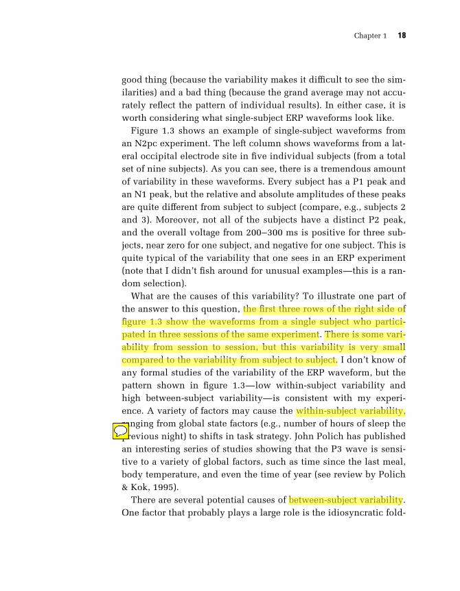
Figure 1.3 shows an example of single-subject waveforms from
an N2pc experiment. The left column shows waveforms from a lat-
eral occipital electrode site in five individual subjects (from a total
set of nine subjects). As you can see, there is a tremendous amount
of variability in these waveforms. Every subject has a P1 peak and
an N1 peak, but the relative and absolute amplitudes of these peaks
are quite different from subject to subject (compare, e.g., subjects 2
and 3). Moreover, not all of the subjects have a distinct P2 peak,
and the overall voltage from 200–300 ms is positive for three sub-
jects, near zero for one subject, and negative for one subject. This is
quite typical of the variability that one sees in an ERP experiment
(note that I didn’t fish around for unusual examples—this is a ran-
dom selection).
What are the causes of this variability? To illustrate one part of
the answer to this question, the first three rows of the right side of
figure 1.3 show the waveforms from a single subject who partici-
pated in three sessions of the same experiment. There is some vari-
ability from session to session, but this variability is very small
compared to the variability from subject to subject. I don’t know of
any formal studies of the variability of the ERP waveform, but the
pattern shown in figure 1.3—low within-subject variability and
high between-subject variability—is consistent with my experi-
ence. A variety of factors may cause the within-subject variability,
ranging from global state factors (e.g., number of hours of sleep the
previous night) to shifts in task strategy. John Polich has published
an interesting series of studies showing that the P3 wave is sensi-
tive to a variety of global factors, such as time since the last meal,
body temperature, and even the time of year (see review by Polich
& Kok, 1995).
There are several potential causes of between-subject variability.
One factor that probably plays a large role is the idiosyncratic fold-
Chapter 1 18

-5µV
+5µV
-100 100 200 300Time Poststimulus (ms)
Subject 6Session 1
Subject 2
Subject 3
Subject 4
Subject 5
Subject 6Session 2
Subject 6Session 3
Average of9 Subjects
Subject 1
Contralateral TargetIpsilateral Target
Figure 1.3 Example of the reliability of averaged ERP waveforms. Data from an N2pc experi-ment are shown for six individual subjects (selected at random from a total set ofnine subjects). Subjects 1–5 participated in a single session, and subject 6 partici-pated in three sessions. The lower right portion of the figure shows the average ofall nine subjects from the experiment. Negative is plotted upward.

ing pattern of the cortex. As I will discuss later in this chapter, the
location and orientation of the cortical generator source of an ERP
component has a huge influence on the size of that component at a
given scalp electrode site. Every individual has a unique pattern of
cortical folding, and the relationship between functional areas and
specific locations on a gyrus or in a sulcus may also vary. Although
I’ve never seen a formal study of the relationship between cortical
folding patterns and individual differences in ERP waveforms, I’ve
always assumed that this is the most significant cause of waveform
variation in healthy young adults (especially in the first 250 ms).
There are certainly other factors that can influence the shape of
the waveforms, including drugs, age, psychopathology, and even
personality. But in experiments that focus on healthy young adults,
these factors probably play a relative small role.
The waveforms in the bottom right portion of figure 1.3 represent
the grand average of the nine subjects in this experiment. A strik-
ing attribute of the grand average waveforms is that the peaks are
smaller than those in most of the single-subject waveforms. This
might seem odd, but it is perfectly understandable. The time point
at which the voltage reaches its peak values for one subject are not
the same as for other subjects, and the peaks in the grand averages
are not at the same time as the peaks for the individual subjects.
Moreover, there are many time points at which the voltage is posi-
tive for some subjects and negative for others. Thus, the grand
average is smaller overall than most of the individual-subject
waveforms. This is a good example of how even simple data pro-
cessing procedures can influence ERP waveforms in ways that
may be unexpected.
There are studies showing that if you average together the pic-
tures of a hundred randomly selected faces, the resulting average
face is quite attractive and looks the same as any other average of
a hundred randomly selected faces from the same population. In
my experience, the same is true for ERP waveforms: Whenever I
run an experiment with a given set of stimuli, the grand average of
ten to fifteen subjects is quite attractive and looks a lot like the
Chapter 1 20

grand average of ten to fifteen different subjects in a similar experi-
ment. Of course the waveform will look different if the stimuli
or task differ substantially between experiments, and occasionally
you will get several subjects with odd-looking waveforms that
make the grand average look a little odd. But usually you will
see a lot of similarity in the grand averages from experiment to
experiment.
Advantages and Disadvantages of the ERP Technique
Comparison with Behavioral Measures
When ERPs were first used to study issues in the domain of cogni-
tive neuroscience, they were primarily used as an alternative to
measurements of the speed and accuracy of motor responses in
paradigms with discrete stimuli and responses. In this context,
ERPs have two distinct advantages. First, an overt response reflects
the output of a large number of individual cognitive processes, and
variations in reaction time (RT) and accuracy are difficult to attri-
bute to variations in a specific cognitive process. ERPs, in contrast,
provide a continuous measure of processing between a stimulus
and a response, making it possible to determine which stage or
stages of processing are affected by a specific experimental manip-
ulation. As an example, consider the Stroop paradigm, in which
subjects must name the color of the ink in which a word is drawn.
Subjects are slower when the word is incompatible with the ink
color than when the ink color and word are the same (e.g., subjects
are slower to say ‘‘green’’ when presented with the word ‘‘red’’
drawn in green ink than when they are presented with the word
‘‘green’’ drawn in green ink). Do these slowed responses reflect
a slowing of perceptual processes or a slowing of response pro-
cesses? It is difficult to answer this question simply by looking
at the behavioral responses, but studies of the P3 wave have
been very useful in addressing this issue. Specifically, it is well
An Introduction to Event-Related Potentials and Their Neural Origins 21

documented that the latency of the P3 wave becomes longer when
perceptual processes are delayed, but several studies have shown
that P3 latency is not delayed on incompatible trials in the Stroop
paradigm, indicating that the delays in RT reflect delays in some
postperceptual stage (see, e.g., Duncan-Johnson & Kopell, 1981).
Thus, ERPs are very useful for determining which stage or stages
of processing are influenced by a given experimental manipulation
(for a detailed set of examples, see Luck, Woodman, & Vogel, 2000).
A second advantage of ERPs over behavioral measures is that
they can provide an online measure of the processing of stimuli
even when there is no behavioral response. For example, much of
my own research involves comparing the processing of attended
versus ignored stimuli, and ERP recordings make it possible to
monitor ‘‘covertly’’ the processing of the ignored stimuli without
requiring subjects to respond to them. Similarly, ERP studies of
language comprehension can assess the processing of a word
embedded in the middle of a sentence at the time the word is pre-
sented rather than relying on a response made at the end of the
sentence. Thus, the ability to covertly monitor the online process-
ing of information is one of the greatest advantages of the ERP tech-
nique. For these reasons, I like to refer to the ERP technique as
‘‘reaction time for the twenty-first century.’’
ERP recordings also have some disadvantages compared to be-
havioral measures. The most obvious disadvantage is that the func-
tional significance of an ERP component is virtually never as clear
as the functional significance of a behavioral response. In most
cases, we do not know the specific biophysical events that underlie
the production of a given ERP response or the consequences of
those events for information processing. In contrast, when a com-
puter records a button-press response, we have a much clearer
understanding of what that signal means. For example, when the
reaction time (RT) in condition A is 30 ms longer than the RT in
condition B, we know that the amount of time required to encode,
process, and act on the stimuli was 30 ms longer in condition A
than in condition B. In contrast, when the peak latency of an ERP
Chapter 1 22

component is 30 ms later in condition A than in condition B,
we can draw no conclusions without relying on a long chain of
assumptions and inferences (see chapter 2 for a discussion of some
problems associated with measuring ERP latencies). Some amount
of inference is always necessary when interpreting physiological
measures of cognition, but some measures are easier to interpret
than others. For example, when we record an action potential, we
have an excellent understanding of the biophysical events that pro-
duced the action potential and the role that action potentials play
in information processing. Thus, the basic signal is more difficult
to interpret in ERP experiments than in behavioral experiments or
in single-unit recordings (but probably no more difficult to inter-
pret than the BOLD [blood oxygen level-dependent] signal in fMRI
experiments).
A second disadvantage of the ERP technique is that ERPs are so
small that it usually requires a large number of trials to measure
them accurately. In most behavioral experiments, a reaction time
difference can be observed with only about twenty to thirty trials
per subject in each condition, whereas ERP effects often require
fifty, a hundred, or even a thousand trials per subject in each con-
dition. I have frequently started designing an ERP experiment and
then given up when I realized that the experiment would require
ten hours of data collection from each subject. Moreover, I rarely
conduct an experiment that requires less than three hours of data
collection from each subject. This places significant limitations on
the types of questions that ERP recordings can realistically answer.
For example, there are some behavioral experiments in which a
given subject can receive only one trial in each condition (e.g., the
inattentional blindness paradigm); experiments of this nature are
not practical with ERP recordings.
Comparison with Other Physiological Measures
Table 1.1 compares the ERP technique (along with its magnetic
counterpart, the event-related magnetic field, or ERMF, technique)
An Introduction to Event-Related Potentials and Their Neural Origins 23
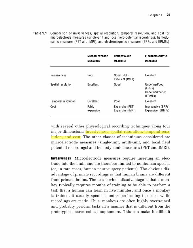
with several other physiological recording techniques along four
major dimensions: invasiveness, spatial resolution, temporal reso-
lution, and cost. The other classes of techniques considered are
microelectrode measures (single-unit, multi-unit, and local field
potential recordings) and hemodynamic measures (PET and fMRI).
Invasiveness Microelectrode measures require inserting an elec-
trode into the brain and are therefore limited to nonhuman species
(or, in rare cases, human neurosurgery patients). The obvious dis-
advantage of primate recordings is that human brains are different
from primate brains. The less obvious disadvantage is that a mon-
key typically requires months of training to be able to perform a
task that a human can learn in five minutes, and once a monkey
is trained, it usually spends months performing the tasks while
recordings are made. Thus, monkeys are often highly overtrained
and probably perform tasks in a manner that is different from the
prototypical naıve college sophomore. This can make it difficult
Table 1.1 Comparison of invasiveness, spatial resolution, temporal resolution, and cost formicroelectrode measures (single-unit and local field-potential recordings), hemody-namic measures (PET and fMRI), and electromagnetic measures (ERPs and ERMFs)
MICROELECTRODE
MEASURES
HEMODYNAMIC
MEASURES
ELECTROMAGNETIC
MEASURES
Invasiveness Poor Good (PET)Excellent (fMRI)
Excellent
Spatial resolution Excellent Good Undefined/poor(ERPs)Undefined/better(ERMFs)
Temporal resolution Excellent Poor Excellent
Cost Fairlyexpensive
Expensive (PET)Expensive (fMRI)
Inexpensive (ERPs)Expensive (ERMFs)
Chapter 1 24

to relate monkey results to the large corpus of human cognitive
experiments. PET experiments are also somewhat problematic
in terms of invasiveness. To avoid exposing subjects to excessive
levels of radiation, each subject can be tested in only a small num-
ber of conditions. In contrast, there is no fundamental restriction
on the amount of ERP or fMRI data that can be collected from a sin-
gle subject.
Spatial and Temporal Resolution Many authors have noted that elec-
tromagnetic measures and hemodynamic measures have comple-
mentary patterns of spatial and temporal resolution, with high
temporal resolution and poor spatial resolution for electromagnetic
measures and poor temporal resolution and high spatial resolution
for hemodynamic measures. ERPs have a temporal resolution of
1 ms or better under optimal conditions, whereas hemodynamic
measures are limited to a resolution of several seconds by the slug-
gish nature of the hemodynamic response. This is over a thousand-
fold difference, and it means that ERPs can easily address some
questions that PET and fMRI cannot hope to address. However,
hemodynamic measures have a spatial resolution in the millimeter
range, which electromagnetic measures cannot match (except, per-
haps, under certain unusual conditions). In fact, as I will discuss in
greater detail later in this chapter and in chapter 7, the spatial res-
olution of the ERP technique is fundamentally undefined, because
there are infinitely many internal ERP generator configurations that
can explain a given pattern of ERP data. Unlike PET and fMRI, it is
not currently possible to specify a margin of error for an ERP local-
ization claim (for the typical case, in which several sources are
simultaneously active). That is, with current techniques, it is im-
possible to know whether a given localization estimate is within
some specific number of millimeters from the actual generator
source. It may someday be possible to definitively localize ERPs,
but at present the spatial resolution of the ERP technique is simply
undefined.
An Introduction to Event-Related Potentials and Their Neural Origins 25

The fact that ERPs are not easily localized has a consequence
that is not often noted. Specifically, the voltage recorded at any
given moment from a single electrode reflects the summed contri-
butions from many different ERP generator sources, each of which
reflects a different neurocognitive process. This makes it extremely
difficult to isolate a single ERP component from the overall ERP
waveform. This is probably the single greatest shortcoming of the
ERP technique, because if you can’t isolate an ERP component
with confidence, it is usually difficult to draw strong conclusions.
Chapter 2 will discuss this issue in greater detail.
Cost ERPs are much less expensive than the other techniques
listed in table 1.1. It is possible to equip a good ERP lab for less
than US $50,000, and the disposable supplies required to test a
single subject are very inexpensive (US $1–3). A graduate student
or an advanced undergraduate can easily carry out the actual
recordings, and the costs related to storing and analyzing the data
are minimal. These costs have dropped a great deal over the past
twenty years, largely due to the decreased cost of computing
equipment. FMRI is fairly expensive, the major costs being person-
nel and amortization of the machine. One session typically costs
US $300–800. PET is exorbitantly expensive, primarily due to the
need for radioactive isotopes with short half-lives and medical
personnel. Single-unit recordings are also fairly expensive due to
the per diem costs of maintaining the monkeys, the cost of the sur-
gical and animal care facilities, and the high level of expertise
required to record electrophysiological data from awake, behaving
monkeys.
Choosing the Right Questions
Given that the ERP technique has both significant advantages and
significant disadvantages, it is extremely important to focus ERP
experiments on questions for which ERPs are well suited. For ex-
ample, ERPs are particularly useful for addressing questions about
Chapter 1 26

which neurocognitive process is influenced by a given manipula-
tion. Conversely, ERPs are poorly suited for asking questions that
require neuroanatomical specificity (except under certain special
conditions; see chapter 7). In addition, it is very helpful to ask
questions that can be addressed with a component that is relatively
easy to isolate (such as the N2pc component and the lateralized
readiness potential) or questions that avoid the problem of identi-
fying a specific ERP component altogether. Unfortunately, there
are no simple rules for determining whether a given question can
be easily answered with ERPs, but chapter 2 discusses a number
of general principles.
The Neural Origins of ERPs
Basic Electrical Concepts
Before reading this section, I would encourage you to read the
appendix, which reviews a few key principles of electricity and
magnetism. You probably learned this material in a physics class
several years ago, but it’s worthwhile to review it again in the con-
text of ERP recordings. You should definitely read it if (a) you’re
not quite sure what the difference between current and voltage is;
or (b) you don’t know Ohm’s law off the top of your head. The
appendix is, I admit, a bit boring. But it’s short and not terribly
complicated.
Electrical Activity in Neurons
To understand the nature of the voltages that can be recorded at the
scalp, it is necessary to understand the voltages that are generated
inside the brain. There are two main types of electrical activity
associated with neurons, action potentials and postsynaptic poten-
tials. Action potentials are discrete voltage spikes that travel from
the beginning of the axon at the cell body to the axon terminals,
An Introduction to Event-Related Potentials and Their Neural Origins 27

where neurotransmitters are released. Postsynaptic potentials are
the voltages that arise when the neurotransmitters bind to recep-
tors on the membrane of the postsynaptic cell, causing ion chan-
nels to open or close and leading to a graded change in the
potential across the cell membrane. If an electrode is lowered into
the intercellular space in a living brain, both types of potentials
can be recorded. It is fairly easy to isolate the action potentials
arising from a single neuron by inserting a microelectrode into
the brain, but it is virtually impossible to completely isolate a sin-
gle neuron’s postsynaptic potentials in an in vivo extracellular
recording. Consequently, in vivo recordings of individual neurons
(‘‘single-unit’’ recordings) measure action potentials rather than
postsynaptic potentials. When recording many neurons simultane-
ously, it is possible to measure either their summed postsynaptic
potentials or their action potentials. Recordings of action potentials
from large populations of neurons are called multi-unit recordings,
and recordings of postsynaptic potentials from large groups of neu-
rons are called local field potential recordings.
In the vast majority of cases, surface electrodes cannot detect
action potentials due to the timing of the action potentials and the
physical arrangement of axons. When an action potential is gener-
ated, current flows rapidly into and then out of the axon at one
point along the axon, and then this same inflow and outflow occur
at the next point along the axon, and so on until the action poten-
tial reaches a terminal. If two neurons send their action potentials
down axons that run parallel to each other, and the action poten-
tials occur at exactly the same time, then the voltages from the two
neurons will summate and the voltage recorded from a nearby
electrode will be approximately twice as large as the voltage
recorded from a single action potential. However, if one neuron
fires slightly after the other, then current at a given spatial location
will be flowing into one axon at the same time that it is flowing out
of the other axon, so they cancel each other and produce a much
smaller signal at the nearby electrode. Because neurons rarely
fire at precisely the same time (i.e., within microseconds of each
Chapter 1 28

other), action potentials in different axons will typically cancel,
and the only way to record the action potentials from a large
number of neurons is to place the electrode near the cell bodies
and to use a very high impedance electrode that is sensitive
only to nearby neurons. As a result, ERPs reflect postsynaptic
potentials rather than action potentials (except under extremely
rare circumstances).
Summation of Postsynaptic Potentials
Whereas the duration of an action potential is only about a
millisecond, postsynaptic potentials typically last tens or even
hundreds of milliseconds. In addition, postsynaptic potentials are
largely confined to the dendrites and cell body and occur essen-
tially instantaneously rather than traveling down the axon at a
fixed rate. Under certain conditions, these factors allow postsynap-
tic potentials to summate rather than cancel, making it possible to
record them at a great distance (i.e., at the scalp).
Very little research has examined the biophysical events that
give rise to scalp ERPs, but figure 1.4 shows the current best guess.
If an excitatory neurotransmitter is released at the apical dendrites
of a cortical pyramidal cell, as shown in figure 1.4A, current will
flow from the extracellular space into the cell, yielding a net nega-
tivity on the outside of the cell in the region of the apical den-
drites. To complete the circuit, current will also flow out of the
cell body and basal dendrites, yielding a net positivity in this area.
Together, the negativity at the apical dendrites and the positivity at
the cell body create a tiny dipole (a dipole is simply a pair of posi-
tive and negative electrical charges separated by a small distance).
The dipole from a single neuron is so small that it would be
impossible to record it from a distant scalp electrode, but under
certain conditions the dipoles from many neurons will summate,
making it possible to measure the resulting voltage at the scalp.
For the summated voltages to be recordable at the scalp, they must
occur at approximately the same time across thousands or millions
An Introduction to Event-Related Potentials and Their Neural Origins 29

Axons fromPresynaptic Cells
Apical Dendrite
Postsynaptic Cell Axon
Basal Dendrites
Cell Body
A
StimulatedRegion
of Cortex
B
EquivalentCurrentDipoleSkull
CortexC
D E
CurrentDipole
MagneticField
Skull
Magnetic FieldLeaving Head
Magnetic FieldEntering Head
Figure 1.4 Principles of ERP generation. (A) Schematic pyramidal cell during neurotransmis-sion. An excitatory neurotransmitter is released from the presynaptic terminals,causing positive ions to flow into the postsynaptic neuron. This creates a net nega-tive extracellular voltage (represented by the ‘‘’’ symbols) in the area of other partsof the neuron, yielding a small dipole. (B) Folded sheet of cortex containing manypyramidal cells. When a region of this sheet is stimulated, the dipoles from the indi-vidual neurons summate. (C) The summated dipoles from the individual neuronscan be approximated by a single equivalent current dipole, shown here as an arrow.The position and orientation of this dipole determine the distribution of positive and
Chapter 1 30

of neurons, and the dipoles from the individual neurons must be
spatially aligned. If the neurons are at random orientations with
respect to each other, then the positivity from one neuron may be
adjacent to the negativity from the next neuron, leading to cancel-
lation. Similarly, if one neuron receives an excitatory neurotrans-
mitter and another receives an inhibitory neurotransmitter, the
dipoles of the neurons will be in opposite directions and will can-
cel. However, if the neurons all have a similar orientation and all
receive the same type of input, their dipoles will summate and
may be measurable at the scalp. This is most likely to occur in cor-
tical pyramidal cells, which are aligned perpendicular to the sur-
face of the cortex, as shown in figure 1.4B.
The summation of the individual dipoles is complicated by the
fact that the cortex is not flat, but instead has many folds. Fortu-
nately, however, physicists have demonstrated that the summation
of many dipoles is essentially equivalent to a single dipole formed
by averaging the orientations of the individual dipoles.2 This aver-
aged dipole is called an equivalent current dipole (ECD). It is im-
portant to note, however, that whenever the individual dipoles are
more than 90 degrees from each other, they will cancel each other
to some extent, with complete cancellation at 180 degrees. For ex-
ample, the Purkinje cells in the cerebellar cortex are beautifully
aligned with each other and oriented perpendicular to the cortical
surface, but the cortical surface is so highly folded that the dipoles
in one small patch of cerebellar cortex will almost always be can-
celled by dipoles in a nearby but oppositely oriented patch, mak-
ing it difficult or impossible to record cerebellar activity from the
scalp.
Figure 1.4 (continued)negative voltages recorded at the surface of the head. (D) Example of a currentdipole with a magnetic field traveling around it. (E) Example of the magnetic fieldgenerated by a dipole that lies just inside the surface of the skull. If the dipole isroughly parallel to the surface, the magnetic field can be recorded as it leaves andenters the head; no field can be recorded if the dipole is oriented radially. Reprintedwith permission from Luck and Girelli 1998. (> 1998 MIT Press.)
An Introduction to Event-Related Potentials and Their Neural Origins 31

Volume Conduction
When a dipole is present in a conductive medium such as
the brain, current is conducted throughout that medium until it
reaches the surface. This is called volume conduction and is illus-
trated in figure 1.4C. The voltage that will be present at any given
point on the surface of the scalp will depend on the position and
orientation of the generator dipole and also on the resistance and
shape of the various components of the head (most notably the
brain, the skull, and the scalp; the eye holes also have an influence,
especially for ERP activity generated in prefrontal cortex).
Electricity does not just run directly between the two poles of
a dipole in a conductive medium, but instead spreads out through
the conductor. Consequently, ERPs spread out as they travel
through the brain. In addition, because electricity tends to follow
the path of least resistance, ERPs tend to spread laterally when
they encounter the high resistance of the skull. Together, these
two factors greatly blur the surface distribution of voltage, and an
ERP generated in one part of the brain can lead to substantial vol-
tages at quite distant parts of the scalp. There are algorithms that
can reduce this blurring, either by estimating the flow of current
or by deblurring the voltage distribution to estimate the voltage
distribution that is present on the brain’s surface (Gevins et al.,
1999; Pernier, Perrin, & Bertrand, 1988). These algorithms can be
very useful, although you should remember that they only elimi-
nate one source of blurring (the skull) and do not indicate the
actual generator location of the ERPs.
Another important point is that electricity travels at nearly the
speed of light. For all practical purposes, the voltages recorded at
the scalp reflect what is happening in the brain at the same mo-
ment in time.
Magnetic Fields
The blurring of voltage caused by the high resistance of the skull
can be largely circumvented by recording magnetic fields instead
Chapter 1 32

of electrical potentials. As figure 1.4D illustrates, an electrical
dipole is always surrounded by a magnetic field, and these fields
summate in the same manner as voltages. Thus, whenever an ERP
is generated, a magnetic field is also generated, running around the
ERP dipole. Moreover, the skull is transparent to magnetism,3 and
the magnetic fields are not blurred by the skull, leading to much
greater spatial resolution than is possible with electrical potentials.
The magnetic equivalent of the EEG is called the magnetoencepha-
logram (MEG), and the magnetic equivalent of an ERP is an event-
related magnetic field (ERMF ).
As figure 1.4E illustrates, a dipole that is perpendicular to the
surface of the scalp will be accompanied by a magnetic field that
leaves the head on one side of the dipole and enters back again on
the other side. If you place a highly sensitive probe called a SQUID
(super-conducting quantum interference device) next to the head,
it is possible to measure the magnetic field as it leaves and reenters
the head. Because magnetic fields are not as smeared out as electri-
cal potentials, they can provide more precise localization. How-
ever, as chapter 7 will discuss, the combination of ERP and ERMF
recordings provides even better localization than ERMF recordings
alone. Unfortunately, magnetic recordings are very expensive be-
cause supercooling is expensive and because an expensive mag-
netically shielded recording chamber is necessary to attenuate the
Earth’s relatively large magnetic field.
ERP Localization
If I tell you the locations and orientations of a set of dipoles in a
volume with a known distribution of conductances, then it would
be possible for you to use a set of equations to compute the distri-
bution of voltage that would be observed for those dipoles. This is
called the forward problem, and it is relatively easy to solve. How-
ever, if I provide you with an observed voltage distribution and ask
you to tell me the locations and orientations of the dipoles, you
will not be able to provide an answer. This is called the inverse
An Introduction to Event-Related Potentials and Their Neural Origins 33
problem, and it is what mathematicians call an ‘‘ill-posed’’ or
‘‘underdetermined’’ problem. This simply means that there is not
just one set of dipoles that can explain a given voltage distribution.
In fact, researchers have known for over 150 years that an infinite
number of different dipole configurations can produce any given
voltage distribution (Helmholtz, 1853) (see also Nunez, 1981; Plon-
sey, 1963). Thus, it is impossible to know with certainty which one
of these configurations is the one that is actually responsible for
producing the observed voltage distribution.
It is possible to use additional constraints to overcome the ill-
posed nature of the inverse problem. However, there is currently
no mathematical technique that is widely accepted as providing a
foolproof means of localizing ERP generator sources. By foolproof,
I mean a technique that can provide a reasonably small and well-
justified margin of error, making it possible to provide a p-value or
likelihood ratio for a statement about the anatomical location of
an ERP effect. For example, I would like to be able to say that the
N2pc component in a particular experiment was generated within
12 mm of the fusiform gyrus and that the probability that this local-
ization is incorrect is less than .05. I am aware of no mathematical
localization technique that allows one to make such statements.
As discussed earlier in this chapter, the main advantages of the
ERP technique are its high temporal resolution, its relatively low
cost, its noninvasiveness, and its ability to provide a covert and
continuous measure of processing. Spatial resolution is simply not
one of the strengths of the ERP technique, and it seems appropriate
to use this technique primarily to address issues that take advan-
tage of its strengths and are not limited by its weaknesses.
Chapter 7 provides more details about ERP localization.
A Summary of Major ERP Components
This section provides a brief description of the ERP components
commonly encountered in cognitive neuroscience research. Some
Chapter 1 34

of these components could justify an entire chapter, but I will
cover just the basics. For more extensive descriptions, see reviews
by Coles and Rugg (1995), Hillyard and Picton (1987), Picton and
Stuss (1980), Naatanen and Picton (1986), and Regan (1989).
Before I start describing the components, however, I’d like to
clarify something that is often confusing to ERP newcomers. Spe-
cifically, ERP components are usually given labels such as P1 and
N1 that refer to their polarity and position within the waveform,
and one must be careful not to assume that these labels are linked
somehow to the nature of the underlying brain activity. Most nota-
bly, sensory components from different modalities that are given
the same label are not usually related in any functional manner:
They just happen to have the same polarity and ordinal position
in the waveform. For example, the auditory P1 and N1 components
bear no particular relationship to the visual P1 and N1 compo-
nents. Some late components such as the P3 wave are largely
modality-independent, but even the P3 wave may have modality-
specific subcomponents (see, e.g., Luck & Hillyard, 1994a). Even
within a single modality, a component labeled N2 in one experi-
ment may not be the same as a component labeled N2 in another
experiment. Some researchers use a bar over the latency of a com-
ponent (e.g., P300) when they are referring to a theoretical entity
rather than simply labeling the observed polarity and latency of a
peak from a particular experiment.
Visual Sensory Responses
C1 The first major visual ERP component is usually called the C1
wave, and it is largest at posterior midline electrode sites. Unlike
most other components, it is not labeled with a P or an N because
its polarity can vary. The C1 wave appears to be generated in area
V1 (primary visual cortex), which in humans is folded into the cal-
carine fissure. The part of area V1 that codes the lower visual field
An Introduction to Event-Related Potentials and Their Neural Origins 35

is on the upper bank of the fissure and the part that codes the
upper visual field is on the lower bank. As a result, the voltage
recorded on the scalp above the calcarine fissure is positive for
stimuli in the lower visual field and negative for stimuli in the up-
per visual field (Clark, Fan, & Hillyard, 1995; Jeffreys & Axford,
1972). The C1 wave is small or positive for stimuli on the horizon-
tal midline, causing it to summate with the P1 wave into a single
wave. Consequently, a distinct C1 wave is usually not observed
unless upper-field stimuli are used to generate a negative C1 wave
(which can be easily distinguished from the positive P1 wave). The
C1 wave typically onsets 40–60 ms poststimulus and peaks 80–100
ms poststimulus, and it is highly sensitive to stimulus parameters,
such as contrast and spatial frequency.
P1 The C1 wave is followed by the P1 wave, which is largest at
lateral occipital electrode sites and typically onsets 60–90 ms post-
stimulus with a peak between 100–130 ms. Note, however, that P1
onset time is difficult to assess accurately due to overlap with the
C1 wave. In addition, P1 latency will vary substantially depending
on stimulus contrast. A few studies have attempted to localize the
P1 wave by means of mathematical modeling procedures, some-
times combined with co-localization with fMRI effects, and these
studies suggest that the early portion of the P1 wave arises from
dorsal extrastriate cortex (in the middle occipital gyrus), whereas a
later portion arises more ventrally from the fusiform gyrus (see Di
Russo et al., 2002). Note, however, that at least thirty distinct vi-
sual areas are activated within the first 100 ms after the onset of a
visual stimulus, and many of these areas presumably contribute to
the voltages recorded in the C1 and P1 latency range. Like the C1
wave, the P1 wave is sensitive to a variations in stimulus parame-
ters, as would be expected given its likely origins in extrastriate vi-
sual cortex. The P1 wave is also sensitive to the direction of spatial
attention (see review by Hillyard, Vogel, & Luck, 1998) and to the
subject’s state of arousal (Vogel & Luck, 2000). Other top-down
variables do not appear to reliably influence the P1 wave.
Chapter 1 36

N1 The P1 wave is followed by the N1 wave. There are several vi-
sual N1 subcomponents. The earliest subcomponent peaks 100–
150 ms poststimulus at anterior electrode sites, and there appear
to be at least two posterior N1 components that typically peak
150–200 ms poststimulus, one arising from parietal cortex and
another arising from lateral occipital cortex. Many studies have
shown that spatial attention influences these components (see
reviews by Hillyard et al., 1998; Mangun, 1995). In addition, the
lateral occipital N1 subcomponent appears to be larger when sub-
jects are performing discrimination tasks than when they are per-
forming detection tasks, which has led to the proposal that this
subcomponent reflects discriminative processing of some sort
(Hopf et al., 2002; Ritter et al., 1979; Vogel & Luck, 2000).
P2 A distinct P2 wave follows the N1 wave at anterior and central
scalp sites. This component is larger for stimuli containing target
features, and this effect is enhanced when the targets are relatively
infrequent (see Luck & Hillyard, 1994a). In this sense, the anterior
P2 wave is similar to the P3 wave. However, the anterior P2 effects
occur only when the target is defined by fairly simple stimulus fea-
tures, whereas P3 effects can occur for arbitrarily complex target
categories. At posterior sites, the P2 wave is often difficult to dis-
tinguish from the overlapping N1, N2, and P3 waves. Conse-
quently, not much is known about the posterior P2 wave.
N170 and Vertex Positive Potential Jeffreys (1989) compared the re-
sponses to faces and non-face stimuli, and he found a difference
between 150 and 200 ms at central midline sites that he named
the vertex positive potential (the electrode site at the very top of
the head is sometimes called the vertex site). Jeffreys noted that
this effect inverted in polarity at more lateral sites, but he did not
have any recordings from electrode sites over inferotemporal cor-
tex. More recent studies from other laboratories that used a broader
range of electrode sites have found that faces elicit a more negative
potential than non-face stimuli at lateral occipital electrode sites,
An Introduction to Event-Related Potentials and Their Neural Origins 37

especially over the right hemisphere, with a peak at approximately
170 ms (Bentin et al., 1996; Rossion et al., 1999). This effect is typ-
ically called the N170 wave. It is likely that the N170 and the ver-
tex positive potential are just the opposite sides of the same dipole
(although this is not a hundred percent certain—see George et al.,
1996; Rossion et al., 1999).
The N170 is later and/or larger for inverted faces than for
upright faces, a hallmark of face specialization. However, an inver-
sion effect is also observed for non-face stimuli when the subjects
have extensive experience viewing these stimuli in an upright
orientations (Rossion et al., 2002). Moreover, other studies have
shown that the vertex positive potential (and presumably the
N170) also occurs for other highly familiar stimuli, such as words
(Schendan, Ganis, & Kutas, 1998). But the face specificity of the
N170 is still a topic of considerable debate (Bentin & Carmel,
2002; Carmel & Bentin, 2002; Rossion, Curran, & Gauthier, 2002).
Auditory Sensory Responses
Very Early Components Under appropriate conditions, it is possible
to observe a sequence of ERP peaks within the first 10 ms of the on-
set of an auditory stimulus. Various sources of evidence indicate
that these peaks arise from various stages along the brainstem audi-
tory pathways, and these peaks are therefore called the brainstem
evoked responses (BERs) or auditory brainstem responses (ABRs).
BERs are extremely useful for assessing auditory pathology, espe-
cially in infants. When my children were born, they were both
given BER screening tests, and it was gratifying to see that a variant
of my main research technique is used for such an important clini-
cal application. The BERs are followed by the midlatency com-
ponents (defined as responses between 10 and 50 ms), which
probably arise at least in part from the medial geniculate nucleus
and the primary auditory cortex. Attention has its first reliable
effects in the midlatency range, but I don’t know of any other top-
Chapter 1 38
down variables that influence auditory activity in this time range.
The midlatency components are followed by the auditory P1 wave
(ca. 50 ms), which is typically largest at frontocentral electrode
sites.
N1 Like the visual N1 wave, the auditory N1 wave has several dis-
tinct subcomponents (see review by Naatanen & Picton, 1987).
These include (1) a frontocentral component that peaks around 75
ms and appears to be generated in the auditory cortex on the dorsal
surface of the temporal lobes, (2) a vertex-maximum potential of
unknown origin that peaks around 100 ms, and (3) a more laterally
distributed component that peaks around 150 ms and appears to be
generated in the superior temporal gyrus. Further fractionation of
the auditory N1 wave is possible (see, e.g., Alcaini et al., 1994).
The N1 wave is sensitive to attention. Although some attention
effects in the N1 latency range reflect the addition of an endoge-
nous component, attention can influence the N1 wave itself (or at
least some N1 subcomponents) (Woldorff et al., 1993).
Mismatch Negativity The mismatch negativity (MMN) is observed
when subjects are exposed to a repetitive train of identical stimuli
with occasional mismatching stimuli (e.g., a sequence with many
800-Hz tones and occasional 1200-Hz tones). The mismatch-
ing stimuli elicit a negative-going wave that is largest at cen-
tral midline scalp sites and typically peaks between 160 and
220 ms. Several other components are sensitive to mismatches
if they are task-relevant, but the MMN is observed even if sub-
jects are not using the stimulus stream for a task (e.g., if they
are reading a book while the stimuli are being presented). How-
ever, the MMN can be eliminated for stimuli presented in one ear
if the subjects focus attention very strongly on a competing se-
quence of stimuli in the other ear (Woldorff, Hackley, & Hillyard,
1991). The MMN is thought to reflect a fairly automatic process
that compares incoming stimuli to a sensory memory trace of pre-
ceding stimuli.
An Introduction to Event-Related Potentials and Their Neural Origins 39

Somatosensory, Olfactory, and Gustatory Responses
The vast majority of cognitive ERP experiments use auditory or vi-
sual stimuli, so I will provide only a brief mention of components
from other modalities. The response to a somatosensory stimulus
begins with one of the rare ERP components (sometimes called
N10) that reflects action potentials rather than postsynaptic poten-
tials, arising from the peripheral nerves. This is followed by a set
of subcortical components (ca. 10–20 ms) and a set of short- and
medium-latency cortical components (ca. 20–100 ms). An N1
wave is then observed at approximately 150 ms, followed by a P2
wave at approximately 200 ms (together, these two peaks are some-
times called the vertex potential ).
It is difficult to record olfactory and gustatory ERP responses,
largely because it is difficult to deliver precisely timed, sudden-
onset stimuli in these modalities (which is necessary when com-
puting averaged ERP waveforms). However, recent studies have
shown that these potentials can be recorded when using appropri-
ate stimulation devices (see, e.g., Ikui, 2002; Wada, 1999).
The N2 Family
The N2 time range has been well studied, and researchers have
identified many clearly different components in this time range
(see extensive discussions in Luck & Hillyard, 1994a; Naatanen &
Picton, 1986). As Naatanen and Picton (1986) describe, a repeti-
tive, nontarget stimulus will elicit an N2 deflection that can be
thought of as the basic N2 (although it doubtless contains several
subcomponents). If other stimuli (often called deviants) are occa-
sionally presented within a repetitive train, a larger amplitude
is observed in the N2 latency range. If these deviants are task-
irrelevant tones, this effect will consist of a mismatch negativity
(visual mismatches do not seem to elicit exactly this sort of auto-
matic mismatch response). If the deviants are task-relevant, then a
somewhat later N2 effect is also observed, called N2b (the mis-
Chapter 1 40
match negativity is sometimes called N2a). This component is
larger for less frequent targets, and it is thought to be a sign of the
stimulus categorization process. Both auditory and visual deviants
will, if task-relevant, elicit an N2b component, but this effect is
largest over central sites for auditory stimuli and over posterior
sites for visual stimuli (Simson, Vaughan, & Ritter, 1977). We do
not really know if the auditory and visual N2b components repre-
sent homologous neural processing functions.
In the visual domain, deviance is often studied spatially rather
than temporally. That is, rather than examining the response to a
deviant item presented within a temporal sequence of homoge-
neous items, one can compare the ERP waveform elicited by a si-
multaneous array of homogeneous items to the ERP waveform
elicited by a simultaneous array that contains several identical
items plus one deviant item. When this is done, one can distin-
guish three N2 components (Luck & Hillyard, 1994a). The first is a
bilateral, anterior response that is present even when the deviant
item is not a target (but it is not as automatic as the MMN because
it is not present unless subjects are looking for deviant targets of
some sort). This is followed by two posterior N2 subcomponents
that are present only if the deviant item is a target (or resembles
the target at first glance). One of these subcomponents is the stan-
dard N2b wave, which is bilateral and probability sensitive. The
second is called N2pc, where the pc is an abbreviation of posterior
contralateral, denoting the fact that this component is observed at
posterior electrode sites contralateral to the location of the target.
The N2pc component is not probability sensitive, and it reflects
the focusing of spatial attention onto the target location (and possi-
bly the suppression of the surrounding nontarget items—see Eimer,
1996; Luck et al., 1997; Luck & Hillyard, 1994b). A contralateral
negativity is also observed during visual working memory tasks,
but it has a more parietally focused scalp distribution and appears
to reflect some aspect of working memory maintenance (Vogel &
Machizawa, 2004).
An Introduction to Event-Related Potentials and Their Neural Origins 41

The P3 Family
There are several distinguishable ERP components in the time
range of the P3 wave. Squires, Squires, and Hillyard (1975) made
the first major distinction, identifying a frontally maximal P3a
component and a parietally maximal P3b component. Both were
elicited by unpredictable, infrequent shifts in tone pitch or in-
tensity, but the P3b component was present only when these
shifts were task-relevant. When ERP researchers (including myself)
refer to the P3 component or the P300 component, they almost al-
ways mean the P3b component (in fact, I will simply use the term
P3 to refer to the P3b component for the rest of this book). Other
studies have shown that an unexpected, unusual, or surprising
task-irrelevant stimulus within an attended stimulus train will elic-
it a frontal P3-like response (e.g., Courchesne, Hillyard, & Galam-
bos, 1975; Polich & Comerchero, 2003; Soltani & Knight, 2000),
but it is not clear whether this response is related to the P3a com-
ponent as Squires, Squires and Hillyard originally described (1975).
For example, Verleger, Jaskowski, and Wauschkuhn (1994) pro-
vided evidence that the P3b component is observed for targets that
are infrequent but are in some sense expected (or ‘‘awaited’’ in the
terms of this paper), whereas the frontal P3 wave is elicited by
stimuli that are truly unexpected or surprising. However, it is not
clear that this frontal P3 is as automatic as the P3a Squires and col-
leagues (1975) observed.
Given the thousands of published P3 experiments, you might
think that we would have a very thorough understanding of the P3
wave. But you’d be wrong! We know a great deal about the effects
of various manipulations on P3 amplitude and latency, but there is
no clear consensus about what neural or cognitive process the P3
wave reflects.4 Donchin (1981) proposed that the P3 wave is some-
how related to a process he called ‘‘context updating’’ (updating
one’s representation of the current environment), but this propo-
sal was not followed by a convincing set of experiments provid-
ing direct support for it. This is probably due to the fact that
we don’t have a good theory of context updating that specifies
Chapter 1 42

how it varies according to multiple experimental manipulations.
If you are interested in the P3 wave, you should probably read
Donchin’s original proposal (Donchin, 1981), Verleger’s exten-
sive critique of the proposal (Verleger, 1988), and the response
of Donchin and Coles to this critique (Donchin & Coles, 1988). In
my own laboratory’s research on attention, we have frequently
assumed that the context-updating proposal is at least approxi-
mately correct, and this has led to a variety of very sensible results
(e.g., Luck, 1998b; Vogel & Luck, 2002; Vogel, Luck, & Shapiro,
1998). But this assumption certainly carries some risk, so you
should be careful in making assumptions about the meaning of the
P3 wave.
Although we do not know exactly what the P3 wave means, we
do know what factors influence its amplitude and latency (for ex-
tensive reviews of the early P3 literature, see Johnson, 1986; Pritch-
ard, 1981; for more recent reviews, see Picton, 1992; Polich, 2004;
Polich & Kok, 1995). The hallmark of the P3 wave is its sensitivity
to target probability: As Duncan-Johnson and Donchin (1977)
described in excruciating detail, P3 amplitude gets larger as target
probability gets smaller. However, it is not just the overall proba-
bility that matters; local probability also matters, because the P3
wave elicited by a target becomes larger when it has been preceded
by more and more nontargets. Moreover, it is the probability of the
task-defined stimulus class that matters, not the probability of the
physical stimulus. For example, if subjects are asked to press a but-
ton when detecting male names embedded in a sequence contain-
ing male and female names, with each individual name occurring
only once, the amplitude of the P3 wave will depend on the rela-
tive proportions of male and female names in the sequence (see
Kutas, McCarthy, & Donchin, 1977). Similarly, if the target is the
letter E, occurring on 10 percent of trials, and the nontargets are
selected at random from the other letters of the alphabet, the target
will elicit a very large P3 wave even though the target letter is
approximately four times more probable than any individual non-
target letter (see Vogel, Luck, & Shapiro, 1998).
An Introduction to Event-Related Potentials and Their Neural Origins 43

P3 amplitude is larger when subjects devote more effort to a task,
leading to the proposal that P3 amplitude can be used as a measure
of resource allocation (see, e.g., Isreal et al., 1980). However, P3
amplitude is smaller when the subject is uncertain of whether a
given stimulus was a target or nontarget. Thus, if a task is made
more difficult, this might increase P3 amplitude by encouraging
subjects to devote more effort to the task, but it might decrease P3
amplitude by making subjects less certain of the category of a given
stimulus. Johnson (1984, 1986) proposed that the variables of
probability (P), uncertainty (U), and resource allocation (R) com-
bine to influence P3 amplitude in the following manner: P3
amplitude ¼ U ðPþ RÞ.Because the P3 wave depends on the probability of the task-
defined category of a stimulus, it is logically necessary that the P3
wave must be generated after the stimulus has been categorized
according to the rules of the task. Consequently, any manipulation
that postpones stimulus categorization (including increasing the
time required for low-level sensory processing or higher-level cate-
gorization) must increase P3 latency. This is logical, and countless
studies have confirmed this prediction. Although P3 latency must
logically depend on the time required to categorize the stimulus, it
is not logically dependent on post-categorization processes; several
studies have shown that P3 latency is not sensitive to the amount
of time required to select and execute a response once a stimulus
has been categorized (see, e.g., Kutas, McCarthy, & Donchin, 1977;
Magliero et al., 1984). For example, if subjects press a left-hand
button when they see the stimulus LEFT and right-hand button
when they see the stimulus RIGHT, P3 latency is no faster or
slower than when they are asked to make a left-hand response for
RIGHT and a right-hand response for LEFT (which is known to in-
crease the time required to perform stimulus-response mapping).
In contrast, if the stimuli are perceptually degraded, then P3 la-
tency is delayed for these stimuli. Thus, one can use P3 latency to
determine if a given experimental manipulation influences the pro-
cesses leading up to stimulus categorization or processes related to
Chapter 1 44

response selection and execution (for an example, see Luck, 1998b;
for contrasting viewpoints, see Leuthold & Sommer, 1998; Ver-
leger, 1997).
Language-Related ERP Components
The best studied language-related component is the N400, first
reported by Kutas and Hillyard (1980) (see also the more recent re-
view by Kutas, 1997). The N400 is negative-going wave that is usu-
ally largest over central and parietal electrode sites, with a slightly
larger amplitude over the right hemisphere than over the left hemi-
sphere. The N400 is typically seen in response to violations of se-
mantic expectancies. For example, if sentences are presented one
word at a time on a video monitor, a large N400 will be elicited by
the last word of the sentence, ‘‘While I was visiting my home town,
I had lunch with several old shirts.’’ Little N400 activity would be
observed if the sentence had ended with ‘‘friends’’ rather than
‘‘shirts.’’ An N400 can also be observed to the second word in a
pair of words, with a large N400 elicited by ‘‘tire . . . sugar’’ and a
small N400 elicited by ‘‘flour . . . sugar.’’ Some N400 activity is pre-
sumably elicited by any content word you read or hear, and rela-
tively infrequent words such as ‘‘monocle’’ elicit larger N400s
than relatively frequent words such as ‘‘milk.’’
Nonlinguistic stimuli can also elicit an N400 (or N400-like activ-
ity), as long as they are meaningful. For example, a line drawing
will elicit an N400 if it is inconsistent with the semantic context
created by a preceding sequence of words or line drawings (Ganis,
Kutas, & Sereno, 1996; Holcomb & McPherson, 1994). However, it
is possible that subjects named the stimuli subvocally, so it is pos-
sible that the N400 component reflects language-specific brain
activity.
Although typically larger at right-hemisphere electrodes than
left-hemisphere electrodes, the N400 appears to be generated pri-
marily in the left temporal lobe. One can explain this apparent dis-
crepancy by assuming that the generator dipole near the base of the
An Introduction to Event-Related Potentials and Their Neural Origins 45

left hemisphere does not point straight upward, but instead points
somewhat medially. Studies of split-brain patients and lesion
patients have shown that the N400 depends on left-hemisphere
activity (Hagoort, Brown, & Swaab, 1996; Kutas, Hillyard, & Gazza-
niga, 1988), and recordings from the cortical surface in neuro-
surgery patients have found clear evidence of N400-like activity in
the left anterior medial temporal lobe (e.g., McCarthy et al., 1995).
Syntactic violations also elicit distinctive ERP components. One
of these is called P600 (see Osterhout & Holcomb, 1992, 1995). For
example, the word ‘‘to’’ elicits a larger P600 in the sentence ‘‘The
broker persuaded to sell the stock’’ than in the sentence ‘‘The bro-
ker hoped to sell the stock.’’ Syntactic violations can also elicit a
left frontal negativity from approximately 300–500 ms, which may
be the same effect observed when wh-questions (e.g., ‘‘What is the
. . .’’) are compared to yes-no questions (e.g., ‘‘Is the . . .’’). Given the
important distinction between syntax and semantics, it should not
be surprising that words that are primarily syntactic in nature elicit
different ERP activity than words with rich semantics. In particu-
lar, function words (e.g., to, with) elicit a component called N280
at left anterior electrode sites, and this component is absent for
content words (e.g., nouns and verbs). In contrast, content words
elicit an N400 that is absent for function words.
Error Detection
In most ERP studies, researchers simply throw out trials with
incorrect behavioral responses. However, by comparing the ERP
waveform elicited on error trials with the ERP waveform elicited
on correct trials, it is possible to learn something about the cause
of the error and the brain’s response following detection of the er-
ror. For example, Gehring et al. (1993) had subjects perform a
speeded response task in which they responded so fast that they
occasionally made errors that were obvious right away (‘‘Oops!
I meant to press the left button!’’). When they compared the
ERPs on correct trials to the ERPs on error trials, they observed a
Chapter 1 46

negative-going deflection at frontal and central electrode sites
beginning just after the time of the response. Gehring et al. called
this deflection the error-related negativity (ERN); it was independ-
ently discovered by Falkenstein et al., (1990), who called it the Ne.
This component is often followed by a positive deflection called
Pe. More recent studies have demonstrated that the ERN can be
elicited by negative feedback following an incorrect response
(Gehring & Willoughby, 2002) or by observing someone else mak-
ing an incorrect response (van Schie et al., 2004).
Most investigators believe that the ERN reflects the activity of
a system that either monitors responses or is sensitive to conflict
between intended and actual responses. Evidence from fMRI and
single-unit recordings suggests that these functions occur in the an-
terior cingulate cortex (Holroyd et al., 2004; Ito et al., 2003), and a
dipole source modeling study showed that the scalp distribution of
the ERN is consistent with a generator source in the anterior cingu-
late (Dehaene, Posner, & Tucker, 1994). However, it is difficult to
localize a broadly distributed component such as the ERN with
much precision on the basis of the observed distribution of voltage.
An intracranial recording study found evidence of an ERN-like re-
sponse in the anterior cingulate, which is more convincing, but
ERN-like responses were also observed at many other cortical sites
in this study. The generator of the ERN is therefore not yet known
with certainty.
Response-Related ERP Components
If subjects are instructed to make a series of occasional manual
responses, with no eliciting stimulus, the responses are preceded
by a slow negative shift at frontal and central electrode sites that
begins up to one second before the actual response. This is called
the bereitschaftspotential (BP) or readiness potential (RP), and it
was independently discovered by Kornhuber and Deecke (1965)
and Vaughn, Costa, and Ritter (1968). The scalp topography of the
readiness potential depends on which effectors will be used to
An Introduction to Event-Related Potentials and Their Neural Origins 47

make the response, with differences between the two sides of the
body and differences within a given side.
The lateralized portion of the readiness potential is called the
lateralized readiness potential (LRP), and it has been widely used
in cognitive studies. As discussed in chapter 2, the LRP is particu-
larly useful because it can be easily isolated from other ERP com-
ponents. That is, because it is lateralized with respect to the hand
making the response, whereas other components are not lateral-
ized, it is easy to tell when a given experimental manipulation has
affected the time or amplitude of the LRP. In contrast, it is difficult
to be certain that a given experimental manipulation has influ-
enced the P3 component rather than some other overlapping com-
ponent, and this is one of the main reasons why it has been so
difficult to determine what cognitive process the P3 component
reflects.
The LRP is generated, at least in part, in motor cortex (Coles,
1989; Miller, Riehle, & Requin, 1992). The most interesting conse-
quence of this is that the LRP preceding a foot movement is oppo-
site in polarity to the LRP preceding a hand movement, reflecting
the fact that the motor cortex representation of the hand is on the
lateral surface of the brain, whereas the representation of the foot
is on the opposed mesial surface. The LRP appears to reflect some
key aspect of response preparation: responses are faster when the
LRP is larger at the moment of stimulus onset, and there is a
threshold level of LRP amplitude beyond which a response will in-
exorably be triggered (Gratton et al., 1988).
The RP and LRP may be present for hundreds of milliseconds
before the response, but other components are more tightly
synchronized to the response. The early view was that a positive-
going deflection is superimposed on the RP beginning 80–90 ms
before the response, followed by a negative-going deflection during
the response and another positive-going deflection after the re-
sponse. However, more recent research has identified many more
movement-related components and subcomponents (see, e.g.,
Nagamine et al., 1994; Shibasaki, 1982).
Chapter 1 48

The contingent negative variation (CNV), described in the brief
history at the beginning of this chapter, should be mentioned again
here because it is partly related to motor preparation. As you will
recall, the CNV is a broad negative deflection between a warning
stimulus and a target stimulus (Walter et al., 1964). When the pe-
riod between the warning and target stimuli is lengthened to sev-
eral seconds, it is possible to see that the CNV actually consists of
a negativity following the warning stimulus, a return to baseline,
and then a negativity preceding the target stimulus (Loveless &
Sanford, 1975; Rohrbaugh, Syndulko, & Lindsley, 1976). The first
negative phase is usually regarded as reflecting processing of
the warning stimulus, and the second negative phase is usually
regarded as reflecting the readiness potential that occurs as the
subject prepares to respond to the target.
Suggestions for Further Reading
The following is a list of journal articles, books, and book chapters
that provide broad and insightful discussions of general ERP
issues.
Coles, M. G. H. (1989). Modern mind-brain reading: Psychophysi-
ology, physiology and cognition. Psychophysiology, 26, 251–
269.
Coles, M. G. H., Smid, H., Scheffers, M. K., & Otten, L. J. (1995).
Mental chronometry and the study of human information
processing. In M. D. Rugg & M. G. H. Coles (Eds.), Electro-
physiology of Mind: Event-Related Brain Potentials and Cogni-
tion. (pp. 86–131). Oxford: Oxford University Press.
Donchin, E. (1979). Event-related brain potentials: A tool in the
study of human information processing. In H. Begleiter (Ed.),
Evoked Brain Potentials and Behavior (pp. 13–88). New York:
Plenum Press.
Donchin, E. (1981). Surprise! . . . Surprise? Psychophysiology, 18,
493–513.
An Introduction to Event-Related Potentials and Their Neural Origins 49

Gaillard, A. W. K. (1988). Problems and paradigms in ERP re-
search. Biological Psychology, 26, 91–109.
Hillyard, S. A., & Picton, T. W. (1987). Electrophysiology of cogni-
tion. In F. Plum (Ed.), Handbook of Physiology: Section 1. The
Nervous System: Volume 5. Higher Functions of the Brain,
Part 2 (pp. 519–584). Bethesda, MD: Waverly Press.
Kutas, M., & Dale, A. (1997). Electrical and magnetic readings of
mental functions. In M. D. Rugg (Ed.), Cognitive Neuroscience.
Studies in Cognition (pp. 197–242). Cambridge, MA: MIT
Press.
Lindsley, D. B. (1969). Average evoked potentials—achievements,
failures and prospects. In E. Donchin & D. B. Lindsley (Eds.),
Average Evoked Potentials: Methods, Results and Evaluations
(pp. 1–43). Washington, D.C.: U.S. Government Printing Office.
Nunez, P. L. (1981). Electric Fields of the Brain. New York: Oxford
University Press.
Picton, T. W., & Stuss, D. T. (1980). The component structure of
the human event-related potentials. In H. H. Kornhuber & L.
Deecke (Eds.), Motivation, Motor and Sensory Processes of the
Brain, Progress in Brain Research (pp. 17–49). North-Holland:
Elsevier.
Sutton, S. (1969). The specification of psychological variables in
average evoked potential experiments. In E. Donchin & D. B.
Lindsley (Eds.), Averaged Evoked Potentials: Methods, Results
and Evaluations (pp. 237–262). Washington, D.C.: U.S. Gov-
ernment Printing Office.
Vaughan, H. G., Jr. (1969). The relationship of brain activity to
scalp recordings of event-related potentials. In E. Donchin &
D. B. Lindsley (Eds.), Average Evoked Potentials: Methods,
Results and Evaluations (pp. 45–75). Washington, D.C.: U.S.
Government Printing Office.
Chapter 1 50

2 The Design and Interpretation of ERP Experiments
This chapter discusses some of the central issues in the design and
interpretation of ERP experiments. Many such issues are unique to
a given research topic (e.g., equating word frequencies in language
experiments), but this chapter will focus on a set of principles that
are common to most cognitive ERP studies.1 Throughout the chap-
ter, I will distill the most significant points into a set of rules and
strategies for designing and analyzing ERP experiments.
It may seem odd to place a chapter on experimental design and
interpretation before the chapters that cover basic issues such as
electrodes and averaging. However, the experimental design is the
most important element of an ERP experiment, and the principles
of experimental design have implications for the more technical
aspects of ERP research.
Waveform Peaks versus Latent ERP Components
The term ERP component refers to one of the most important and
yet most nebulous concepts in ERP research. An ERP waveform
unambiguously consists of a series of peaks and troughs, but these
voltage deflections reflect the sum of several relatively indepen-
dent underlying or latent components. It is extremely difficult to
isolate the latent components so that they can be measured inde-
pendently, and this is the single biggest roadblock to designing
and interpreting ERP experiments. Consequently, one of the keys
to successful ERP research is to distinguish between the observable
peaks of the waveform and the unobservable latent components.
This section describes several of the factors that make it difficult
to assess the latent components, along with a set of ‘‘rules’’ for

avoiding misinterpreting the relationship between the observable
peaks and the underlying components.
Voltage Peaks Are not Special
Panels A–C in figure 2.1 illustrate the relationship between the vis-
ible ERP peaks and the latent ERP components. Panel A shows an
ERP waveform, and panel B shows a set of three latent ERP compo-
nents that, when summed together, equal the ERP waveform in
panel A. When several voltages are present simultaneously in a
conductor such as the brain, the combined effect of the individual
voltages is exactly equal to their sum, so it is quite reasonable to
think about ERP waveforms as an expression of several summed
latent components. In most ERP experiments, the researchers want
to know how an experimental manipulation influences a specific
latent component, but we don’t have direct access to the latent
components and must therefore make inferences about them from
the observed ERP waveforms. This is more difficult than it might
seem, and the first step is to realize that the maximum and mini-
mum voltages (i.e., the peaks) in an observed ERP waveform are
not necessarily a good reflection of the latent components. For ex-
ample, the peak latency of peak 1 in the ERP waveform in panel
A is much earlier than the peak latency of component C1 in
panel B. This leads to our first rule of ERP experimental design
and interpretation:
Rule 1. Peaks and components are not the same thing. There is
nothing special about the point at which the voltage reaches a local
maximum.
In light of this fundamental rule, I am always amazed at how
often researchers use peak amplitude and peak latency to measure
the magnitude and timing of ERP components. These measures
often provide a highly distorted view of the amplitude and timing
of the latent components, and better techniques are available for
quantifying ERP data (see chapter 5).
Chapter 2 52
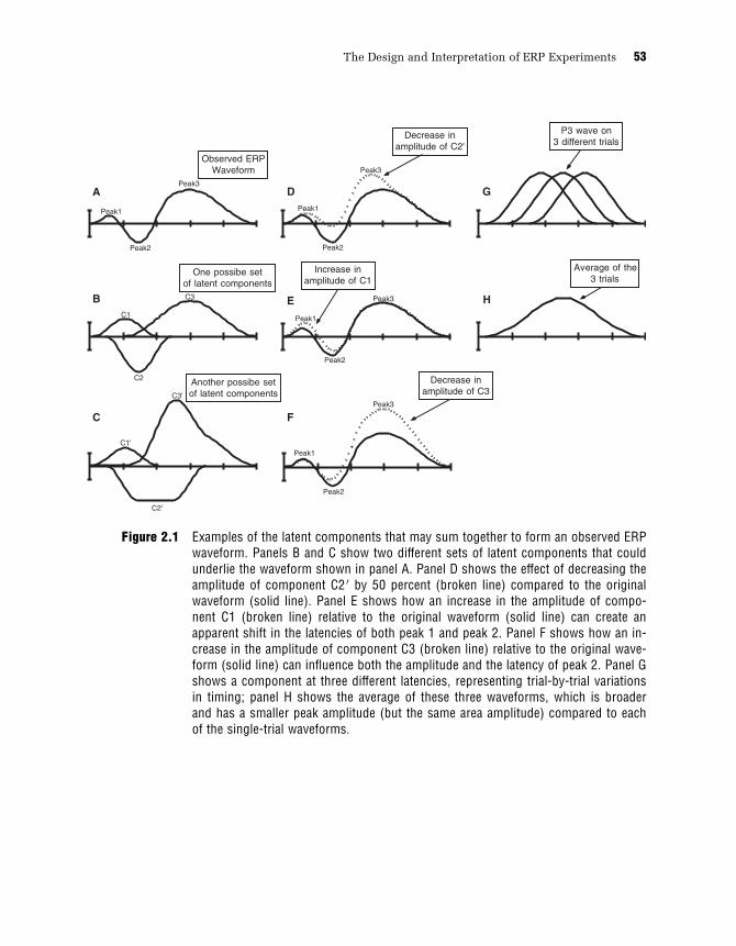
C1
C2
Peak1
Peak1
Peak1
Peak2
Peak2
Peak2
Peak3
Peak3
Peak3
C3
C1'
C2'
C3'
A D
B E
C F
G
H
Peak1
Peak2
Peak3
Decrease inamplitude of C2'
Observed ERPWaveform
One possibe setof latent components
Another possibe setof latent components
P3 wave on3 different trials
Average of the3 trials
Decrease inamplitude of C3
Increase inamplitude of C1
Figure 2.1 Examples of the latent components that may sum together to form an observed ERPwaveform. Panels B and C show two different sets of latent components that couldunderlie the waveform shown in panel A. Panel D shows the effect of decreasing theamplitude of component C2 0 by 50 percent (broken line) compared to the originalwaveform (solid line). Panel E shows how an increase in the amplitude of compo-nent C1 (broken line) relative to the original waveform (solid line) can create anapparent shift in the latencies of both peak 1 and peak 2. Panel F shows how an in-crease in the amplitude of component C3 (broken line) relative to the original wave-form (solid line) can influence both the amplitude and the latency of peak 2. Panel Gshows a component at three different latencies, representing trial-by-trial variationsin timing; panel H shows the average of these three waveforms, which is broaderand has a smaller peak amplitude (but the same area amplitude) compared to eachof the single-trial waveforms.
The Design and Interpretation of ERP Experiments 53
Peak Shapes Are not the Same as Component Shapes
Panel C of figure 2.1 shows another set of latent components that
also sum together to equal the ERP waveform shown in panel A. In
this case, the relatively short duration and hill-like shape of peak 2
in panel A bears little resemblance to the long duration, boxcar-
like component C2 0 in panel C. This leads to our second rule:
Rule 2. It is impossible to estimate the time course or peak
latency of a latent ERP component by looking at a single ERP
waveform—there may be no obvious relationship between the
shape of a local part of the waveform and the underlying
components.
Violations of this rule are especially problematic when compar-
ing two or more ERP waveforms. For example, consider the ERP
waveforms in panel D of figure 2.1. The solid waveform represents
the sum of the three latent components in panel C (which is the
same as the ERP waveform in panel A), and the dashed waveform
shows the effects of decreasing component C2 0 by 50 percent. To
make this a bit more concrete, you can think of these waveforms
as the response to an attended stimulus and an unattended stimu-
lus, respectively, such that ignoring the stimulus leads to a 50 per-
cent decline in the amplitude of component C2 0. Without knowing
the underlying component structure, it would be tempting to con-
clude from the ERP waveforms shown in panel D that the un-
attended stimulus elicits not only a decrease in the amplitude of
component C2 0 but also an increase in the amplitude of component
C1 0 and a decrease in the latency and an increase in the amplitude
of component C3 0. In other words, researchers often interpret an ef-
fect that overlaps with multiple peaks in the ERP waveform as
reflecting changes in multiple underlying components, but this in-
terpretation is often incorrect. Alternatively, you might conclude
from the waveforms in panel D that the attentional manipulation
adds an additional, long-duration component that would not other-
wise be present at all. This would also be an incorrect conclusion,
which leads us to:
Chapter 2 54

Rule 3. It is dangerous to compare an experimental effect (i.e.,
the difference between two ERP waveforms) with the raw ERP
waveforms.
Rule 3 applies to comparisons of scalp distribution as well as
comparisons of timing. That is, it is not usually appropriate to
compare the scalp distribution of an experimental effect with the
scalp distribution of the raw ERP waveform. For example, imagine
you found that words elicited a more negative response in the N1
latency range than nonwords. To determine whether this effect
reflects a change in the amplitude of the exogenous N1 or the addi-
tion of a word-specific neural process, it would be tempting to cal-
culate a word-minus-nonword difference wave and compare the
scalp distribution of this difference wave (in the N1 latency range)
to the scalp distribution of the N1 elicited by nonwords. If the
scalp distributions were found to be different, one might conclude
that the effect represents the addition of endogenous, word-specific
brain activity. But this conclusion would be unwarranted. The
nonword-elicited N1 scalp distribution certainly represents over-
lapping activity from multiple latent components, and a different
scalp distribution would be expected for the word-minus-nonword
difference wave if a subset of these latent components were larger
(or smaller) for words than for nonwords. Moreover, a change in
the latency of one of the latent components would also lead to dif-
ferences in scalp distribution. Thus, if the scalp distribution differs
between two conditions, the only certain conclusion is that the ex-
perimental manipulation does not simply change the amplitude of
all components proportionately.
This raises an important point about the relationship between
amplitude and latency. Although the amplitude and latency of a
latent component are conceptually independent, amplitude and la-
tency often become confounded when measuring ERP waveforms.
This occurs because the latent components overlap in time. Con-
sider, for example, the relatively straightforward correspondence be-
tween the peaks in panel A of figure 2.1 and the latent components
The Design and Interpretation of ERP Experiments 55

in panel B of the figure. Panel E of the figure shows the effects of
increasing the amplitude of the first latent component on the
summed ERP activity. When the amplitude of component A
is increased by 50 percent, this creates an increase in the latency
of both peak 1 and peak 2 in the summed waveform, and it also
causes a decrease in the peak amplitude of peak 2. Panel F illus-
trates the effect of doubling the amplitude of the component C3,
which causes a decrease in the amplitude and the latency of the
second peak. Once again, this shows how the peak voltage in a
given time range is a poor measure of the underlying ERP compo-
nents in that latency range. This leads to our next rule:
Rule 4. Differences in peak amplitude do not necessarily corre-
spond with differences in component size, and differences in peak
latency do not necessarily correspond with changes in component
timing.
Distortions Caused by Averaging
In the vast majority of ERP experiments, the ERP waveforms are
isolated from the EEG by means of signal-averaging procedures. It
is tempting to think of signal-averaging as a process that simply
attenuates the nonspecific EEG, allowing us to see what the single-
trial ERP waveforms look like. However, to the extent that the
single-trial waveform varies from trial to trial, the averaged ERP
may provide a distorted view of the single-trial waveforms, partic-
ularly when component latencies vary from trial to trial. Panels G
and H of figure 2.1 illustrate this distortion. Panel G illustrates
three single-trial ERP waveforms (without any EEG noise), with
significant latency differences across trials, and panel H shows the
average of those three single-trial waveforms. The averaged wave-
form differs from the single-trial waveforms in two significant
ways. First, it is smaller in peak amplitude. Second, it is more
spread out in time. In addition, even though the waveform in panel
H is the average of the waveforms in panel G, the onset time of the
Chapter 2 56
averaged waveform in panel H reflects the onset time of the earliest
single-trial waveform and not the average onset time. This leads to
our next rule:
Rule 5. Never assume that an averaged ERP waveform accurately
represents the individual waveforms that were averaged together.
In particular, the onset and offset times in the averaged waveform
will represent the earliest onsets and latest offsets from the individ-
ual trials or individual subjects that contribute to the average.
Fortunately, it is often possible to measure ERPs in a way
that avoids the distortions created by the signal-averaging process.
For example, the area under the curve in the averaged waveform
shown in panel H is equal to the average of the area under the
single-trial curves in panel G. In most cases, measurements of area
amplitude (or mean amplitude) are superior to measurements of
peak amplitude. Similarly, it is possible to find the time point that
divides the area into two equal halves, and this can be a better
measure of latency than peak measures (for more details, see chap-
ter 6).
It is worth mentioning that a very large number of published ERP
experiments have violated the five rules presented so far. There is
no point in cataloging the cases (especially given that the list would
include some of my own papers). However, violations of these
rules significantly undermine the strength of the conclusions that
one can draw from these experiments. For new students of the
ERP technique, it would be worth reading a large set of ERP papers
and trying to identify both violations of these rules and methods
for avoiding the pitfalls that the rules address.
What Is an ERP Component?
So how can we accurately assess changes in latent components
on the basis of the observed ERP waveforms? Ideally, we would
like to be able to take an averaged ERP waveform and use some
simple mathematical procedure to recover the actual waveforms
The Design and Interpretation of ERP Experiments 57

corresponding to the components that sum together to create the
recorded ERP waveform. We could then measure the amplitude
and the latency of the isolated components, and changes in one
component would not influence our measurement of the other
components. Unfortunately, just as there are infinitely many gener-
ator configurations that could give rise to a given ERP scalp distri-
bution, there are infinitely many possible sets of latent components
that could be summed together to give rise to a given ERP wave-
form. In fact, this is the basis of Fourier analysis: any waveform
can be decomposed into the sum of a set of sine waves. Similarly,
techniques such as principal components analysis (PCA) and inde-
pendent components analysis (ICA) use the correlational structure
of a data set to derive a set of basis components that can be added
together to create the observed waveforms (for more information,
see Donchin & Heffley, 1978; Makeig et al., 1997). Localization
techniques can also be used to compute component waveforms at
the site of each ERP generator source. Unfortunately, none of these
techniques has yet been perfected, as discussed in this section.
All techniques for estimating the latent components are based on
assumptions about what a component is. In the early days of ERP
research, a component was defined primarily on the basis of its po-
larity, latency, and general scalp distribution. For example, the P3a
and P3b components were differentiated on the basis of the earlier
peak latency and more frontal distribution of the P3a component
relative to the P3b component. However, polarity, latency, and
scalp distribution are superficial features that don’t really capture
the essence of a component. For example, the peak latency of the
P3b component may vary by hundreds of milliseconds depending
on the difficulty of the target-nontarget discrimination (Johnson,
1986), and the scalp distribution of the auditory N1 wave depends
on the pitch of the eliciting stimulus in a manner that corresponds
with the tonotopic map of auditory cortex (Bertrand, Perrin, & Per-
nier, 1991). Even polarity may vary: the C1 wave, which is gener-
ated in primary visual cortex, is negative for upper-field stimuli
and positive for lower-field stimuli due to the folding pattern
Chapter 2 58

of this cortical area (Clark, Fan, & Hillyard, 1995). Consequently,
many investigators now define components in terms of a combina-
tion of computational function and neuroanatomical generator site
(see, e.g., Naatanen & Picton, 1987). Consistent with this approach,
my own definition of the term ERP component is:
Scalp-recorded neural activity that is generated in a given
neuroanatomical module when a specific computational operation
is performed.
By this definition, a component may occur at different times
under different conditions, as long as it arises from the same
module and represents the same cognitive function (e.g., the
encoding of an item into working memory in a given brain area
may occur at different delays following the onset of a stimulus be-
cause of differences in the amount of time required to identify the
stimulus and decide that it is worth storing in working memory).
The scalp distribution and polarity of a component may also vary
according to this definition, because the same cognitive function
may occur in different parts of a cortical module under different
conditions (e.g., when a visual stimulus occurs at different loca-
tions and therefore stimulates different portions of a topographi-
cally mapped area of visual cortex). It is logically possible for two
different cortical areas to accomplish exactly the same cognitive
process, but this probably occurs only rarely and would lead to a
very different pattern of voltages, and so this would not usually be
considered a single ERP component.2
Techniques such as PCA and ICA use the correlational struc-
ture of an ERP data set to define a set of components, and these
techniques therefore derive components that are based on func-
tional relationships. Specifically, different time points are grouped
together as part of a single component to the extent they tend to
vary in a correlated manner, as would be expected for time points
that reflect a common cognitive process. The PCA technique, in
particular, is problematic because it does not yield a single, unique
set of underlying components without additional assumptions (see,
The Design and Interpretation of ERP Experiments 59

e.g., Rosler & Manzey, 1981). That is, PCA really just provides a
means of determining the possible set of latent component wave-
shapes, but additional assumptions are necessary to decide on one
set of component waveshapes (and there is typically no way to ver-
ify that the assumptions are correct). The ICA technique appears
to be a much better approach, because it uses both linear and non-
linear relationships to define the components. However, because
ICA is a new technique, it remains to be seen whether it will turn
out to be a generally useful means of identifying latent compo-
nents. In particular, any technique based on identifying correlated
versus independent time points will be limited by that fact that
when two separate cognitive processes covary, they may be cap-
tured as part of a single component even if they occur in very dif-
ferent brain areas and represent different cognitive functions. For
example, if all of the target stimuli in a given experimental para-
digm are transferred into working memory, an ERP component
associated with target detection may always be accompanied by a
component associated with working memory encoding, and this
may lead ICA to group them together as a single component. More-
over, both PCA and ICA fail when latencies vary across conditions.
Thus, correlation-sensitive techniques may sometimes be useful
for identifying latent ERP components, but it remains to be seen
whether these techniques are generally effective under typical ex-
perimental conditions.
Techniques for localizing ERPs can potentially provide measures
of the time course of activity within anatomically defined regions.
In fact, this aspect of ERP localization techniques might turn out
to be just as important as the ability to determine the neuroanatom-
ical locus of an ERP effect. However, as discussed in chapters 1
and 7, there are no general-purpose and foolproof techniques for
definitively localizing ERPs at present, and we may never have
techniques that allow direct and accurate ERP localization. Thus,
this approach to identifying latent ERP components is not gener-
ally practical at the present time.
Chapter 2 60

In addition to mathematical techniques for determining the la-
tent components in an ERP waveform, it is also possible to use the
world’s most powerful pattern analyzer, the human brain. As you
gain expertise with specific components and with ERPs in general,
you will be able to look at a set of ERP data and make a reasonably
good inference about the underlying component structure. This
involves considering how the peaks interact with each other across
time and across electrode locations and coming up with an inter-
pretation that is consistent with the observed waveforms. Kramer
(1985) studied this formally, creating a set of simulated ERP wave-
forms and asking a set of graduate students and research assistants
to make judgments about them. He found that these individuals
did a good job of recovering the underlying component structure
from the waveforms, but that this depended on the observer’s level
of experience. Thus, you should become skilled at determining
the component structure of ERP waveforms over time. This is
an important skill, because you will use your assessment of the la-
tent components to guide your measurement and analysis of the
waveforms.
Avoiding Ambiguities in Interpreting ERP Components
The preceding sections of this chapter are rather depressing, be-
cause it seems like there is no perfectly general means for measur-
ing latent components from observed ERP waveforms. This is a
major problem, because many ERP experiments make predictions
about the effects of some experimental manipulation on a given
component, and the conclusions of these experiments are valid
only if the observed effects really reflect changes in that compo-
nent. For example, the N400 component is widely regarded as a
sensitive index of the degree of mismatch between a word and a
previously established semantic context, and it would be nice to
use this component to determine which of two sets of words sub-
jects perceive as being more incongruous. If two sets of words elicit
The Design and Interpretation of ERP Experiments 61
different ERP waveforms, it is necessary to know whether this ef-
fect reflects a larger N400 for one set or a larger P3 for the other
set; otherwise, it is impossible to determine whether the two sets
of words differ in terms of semantic mismatch or some other vari-
able (i.e., a variable to which the P3 wave is sensitive). Here I will
describe six strategies for minimizing factors that lead to ambigu-
ous relationships between the observed ERP waveforms and the la-
tent components.
Strategy 1. Focus on a Specific Component
The first strategy is to focus a given experiment on only one or
perhaps two ERP components, trying to keep as many other com-
ponents as possible from varying across conditions. If fifteen dif-
ferent components vary, you will have a mess, but variations in a
single component are usually tractable. Of course, sometimes a
‘‘fishing expedition’’ is necessary when using a new paradigm,
but don’t count on obtaining easily interpretable results in such
cases.
Strategy 2. Use Well-Studied Experimental Manipulations
It is usually helpful to examine a well-characterized ERP compo-
nent under conditions that are as similar as possible to conditions
in which that component has previously been studied. For exam-
ple, when Marta Kutas first started recording ERPs in language
paradigms, she focused on the P3 wave and varied factors such as
‘‘surprise value’’ that had previously been shown to influence the
P3 wave in predictable ways. Of course, when she used semantic
mismatch to elicit surprise, she didn’t observe the expected P3
wave but instead discovered the N400 component. However, the
fact that her experiments were so closely related to previous P3
experiments made it easy to determine that the effect she observed
was a new negative-going component and not a reduction in the
amplitude of the P3 wave.
Chapter 2 62

Strategy 3. Focus on Large Components
When possible, it is helpful to study large components such as P3
and N400. When the component of interest is very large compared
to the other components, it will dominate the observed ERP wave-
form, and measurements of the corresponding peak in the ERP
waveform will be relatively insensitive to distortions from the
other components.
Strategy 4. Isolate Components with Difference Waves
It is often possible to isolate the component of interest by creating
difference waves. For example, imagine that you are interested
in assessing the N400 for two different noun types, count nouns
(e.g., cup) and mass nouns (e.g., water). The simple approach to
this might be to present one word per second, with count nouns
and mass nouns randomly intermixed. This would yield two ERP
waveforms, one for count nouns and one for mass nouns, but
it would be difficult to know if any differences observed between
the count noun and mass noun waveforms were due to differ-
ence in N400 amplitude or due to differences in some other ERP
component.
To isolate the N400, you could redesign the experiment so that
each trial contained a sequence of two words, a context word and
a target word, with count noun target word on some trials and a
mass noun target word on others. In addition, the context and tar-
get words would sometimes be semantically related and sometimes
be semantically unrelated. You would then have four types of trial
types:
Count noun, related to context word (e.g., ‘‘plate . . . cup’’)
Mass noun, related to context word (e.g., ‘‘rain . . . water’’)
Count noun, unrelated to context word (e.g., ‘‘sock . . . cup’’)
Mass noun, unrelated to context word (e.g., ‘‘garbage . . . water’’)
You could then isolate the N400 by constructing difference
waves in which the ERP waveform elicited by a given word when
The Design and Interpretation of ERP Experiments 63

it was preceded by a semantically related context word is sub-
tracted from the ERP waveform elicited by that same word when
preceded by a semantically unrelated context word. Separate dif-
ference waves would be constructed for count nouns and mass
nouns (unrelated minus related count nouns and unrelated minus
related mass nouns). Each of these difference waves should be
dominated by a large N400 component, with little or no contri-
bution from other components (because most other components
aren’t sensitive to semantic mismatch). You could then see if the
N400 was larger in the count noun difference wave or in the mass
noun difference wave (I describe a real application of this general
approach at the very end of this chapter—see Vogel, Luck, &
Shapiro, 1998 for details).
Although this approach is quite powerful, it has some limita-
tions. First, difference waves constructed in this manner may con-
tain more than one ERP component. For example, there may be
more than one ERP component that is sensitive to the degree of
semantic mismatch, so an unrelated-minus-related difference wave
might consist of two or three components rather than just one.
However, this is still a vast improvement over the raw ERP wave-
forms, which probably contain at least ten different components.
The second limitation of this approach is that it is sensitive to
interactions between the variable of interest (e.g., count nouns
versus mass nouns) and the factor that is varied to create the dif-
ference waves (e.g., semantically related versus unrelated word
pairs). If, for example, the N400 amplitude is 1 mV larger for count
nouns than for mass nouns, regardless of the degree of semantic
mismatch, then count noun difference waves will be identical
to the mass noun difference waves. Fortunately, when two factors
influence the same ERP component, they are likely to interact mul-
tiplicatively. For example, N400 amplitude might be 20 percent
greater for count nouns than for mass nouns, leading to a larger ab-
solute difference in N400 amplitude when the words are unrelated
to the context word than when they are related. Of course, the
interactions could take a more complex form that would lead to
Chapter 2 64

unexpected results. For example, count nouns could elicit a larger
N400 than mass nouns when the words are unrelated to the con-
text word, but they might elicit a smaller N400 when the words
are related to the context word. Thus, although difference waves
can be very helpful in isolating specific ERP components, care is
necessary when interpreting the results.
I should also mention that the signal-to-noise ratio of a differ-
ence wave will be lower than those of the original ERP wave-
forms. Specifically, if the original waveforms have similar noise
levels, then the noise in the difference wave will be larger by a
factor of the square root of two (i.e., approximately 40 percent
larger).
Strategy 5. Focus on Components That Are Easily Isolated
The previous strategy advocated using difference waves to isolate
ERP components, and one can refine this by focusing on certain
ERP components that are relatively easy to isolate. The best ex-
ample of this is the lateralized readiness potential (LRP), which
reflects movement preparation and is distinguished by its con-
tralateral scalp distribution. Specifically, the LRP in a given hemi-
sphere is more negative when a movement of the contralateral
hand is being prepared than when a movement of the ipsilateral
hand is being prepared, even if the movements are not executed.
In an appropriately designed experiment, only the motor prepara-
tion will lead to lateralized ERP components, making it possible to
form difference waves in which all ERPs are subtracted away ex-
cept for those related to lateralized motor preparation (see Coles,
1989; Coles et al., 1995). Similarly, the N2pc component for a
given hemisphere is more negative when attention is directed to
the contralateral visual field than when it is directed to the ipsi-
lateral field, even when the evoking stimulus is bilateral. Because
most of the sensory and cognitive components are not lateralized
in this manner, the N2pc can be readily isolated (see, e.g., Luck et
al., 1997; Woodman & Luck, 2003).
The Design and Interpretation of ERP Experiments 65

Strategy 6. Component-Independent Experimental Designs
The best strategy is to design experiments in such a manner that it
does not matter which latent ERP component is responsible for the
observed changes in the ERP waveforms. For example, Thorpe and
colleagues (1996) conducted an experiment in which they asked
how quickly the visual system can differentiate between different
classes of objects. To answer this question, they presented subjects
with two classes of photographs, pictures that contained animals
and pictures that did not. They found that the ERPs elicited by
these two classes of pictures were identical until approximately
150 ms, at which point the waveforms diverged. From this experi-
ment, it is possible to infer that the brain can detect the presence of
an animal in a picture by 150 ms, at least for a subset of pictures
(note that the onset latency represents the trials and subjects with
the earliest onsets and not necessarily the average onset time).
This experimental effect occurred in the time range of the N1 com-
ponent, but it may or may not have been a modulation of that com-
ponent. Importantly, the conclusions of this study do not depend
at all on which latent component the experimental manipulation
influenced. Unfortunately, it is rather unusual to be able to answer
a significant question in cognitive neuroscience using ERPs in a
component-independent manner, but one should use this approach
whenever possible. I will provide additional examples later in this
chapter.
Avoiding Confounds and Misinterpretations
The problem of assessing latent components on the basis of
observed ERP waveforms is usually the most difficult aspect of
the design and interpretation of ERP experiments, and this prob-
lem is particularly significant in ERP experiments. There are other
significant experimental design issues that are applicable to a wide
spectrum of techniques, but are particularly salient in ERP experi-
ments; these will be the focus of this section.
Chapter 2 66

The most fundamental principle of experimentation is to make
sure that a given experimental effect has only a single possible
cause. One part of this principle is to avoid confounds, but a
subtler part is to make sure that the experimental manipulation
doesn’t have secondary effects that are ultimately responsible for
the effect of interest. For example, imagine that you observe that
the mass of a beaker of hot water is less than the mass of a beaker
of cold water. This might lead to the erroneous conclusion that hot
water has a lower mass than cool water, even though the actual ex-
planation is that some of the heated water turned to steam, which
escaped through the top of the beaker. To reach the correct con-
clusion, it is necessary to seal the beakers so that water does not
escape. Similarly, it is important to ensure that experimental
manipulations in ERP experiments do not have unintended side
effects that lead to an incorrect conclusion.
To explore the most common problems that occur in ERP experi-
ments, let’s consider a thought experiment that examines the effects
of stimulus discriminability on P3 amplitude. In this experiment,
letters of the alphabet are presented foveally at a rate of one per
second and the subject is required to press a button whenever the
letter Q is presented. A Q is presented on 10 percent of trials and
a randomly selected non-Q letter is presented on the other 90 per-
cent. In addition, the letter Q never occurs twice in succession. In
one set of trial blocks, the stimuli are bright and therefore easy
to discriminate (the bright condition), and in another set of trial
blocks the stimuli are very dim and therefore difficult to discrimi-
nate (the dim condition).
There are several potential problems with this seemingly
straightforward experimental design, mainly due to the fact that
the target letter (Q) differs from the nontarget letters in several
ways. First, the target category occurs on 10 percent of trials
whereas the nontarget category occurs on 90 percent of trials. This
is one of the two intended experimental manipulations (the other
being target discriminability). Second, the target and nontarget
The Design and Interpretation of ERP Experiments 67

letters are different from each other. Not only is the target letter a
different shape from the nontarget letters—and might therefore
elicit a somewhat different ERP waveform—the target letter also
occurs more frequently than any of the individual nontarget letters.
To the extent that the visual system exhibits long-lasting and
shape-specific adaptation to repeated stimuli, it is possible that
the response to the letter Q will become smaller than the response
to the other letters. These physical stimulus differences probably
won’t have a significant effect on the P3 component, but they could
potentially have a substantial effect on earlier components (for a
detailed example, see experiment 4 of Luck & Hillyard, 1994a).
An important principle of ERP experimental design that I
learned from Steve Hillyard is that you should be very careful to
avoid confounding differences in psychological factors with subtle
differences in stimulus factors. In this example experiment, for ex-
ample, the probability difference between the target and nontarget
letters—which is intended to be a psychological manipulation—
is confounded with shape differences and differences in sensory
adaptation. Although such confounds primarily influence sensory
responses, these sensory responses can last for hundreds of milli-
seconds, and you will always have the nagging suspicion that your
P3 or N400 effects reflect a sensory confound rather than your in-
tended psychological manipulation. The solution to this confound
is to make sure that your manipulations of psychological variables
are not accompanied by any changes in the stimuli (including the
sequential context of the stimulus of interest). This is typically ac-
complished by using the same stimulus sequences in two or more
conditions and using verbal or written instructions to manipulate
the subject’s task. A statement that is prominently displayed on a
wall in my laboratory summarizes this:
The Hillyard Principle—Always compare ERPs elicited by the
same physical stimuli, varying only the psychological conditions.
Of course, implementing the Hillyard Principle is not always
possible. For example, you may want to examine the ERPs elicited
Chapter 2 68
by closed-class words (articles, prepositions, etc.) and open-class
words (nouns, verbs, etc.); these are by definition different stimuli.
But you should be very careful that any ERP differences reflect the
psychological differences between the stimuli and not low-level
physical differences (e.g., word length). I can tell you from experi-
ence that every time I have violated the Hillyard Principle, I have
later regretted it and ended up running a new experiment. Box 2.1
provides two examples of confounds that somehow crept into my
own experiments.
A third difference between the target and nontarget letters is that
subjects make a response to the targets and not to the nontargets.
Consequently, any ERP differences between the targets and non-
targets could be contaminated by motor-related ERP activity. A
fourth difference between the targets and the nontargets is that
because the target letter never occurred twice in succession, the
target letter was always preceded by a nontarget letter, whereas
nontarget letters could be preceded by either targets or nontargets.
This is a common practice, because the P3 to the second of two
targets tends to be reduced in amplitude. This is usually a bad
idea, however, because the response to a target is commonly very
long-lasting and extends past the next stimulus and therefore influ-
ences the waveform recorded for the next stimulus. Thus, there
may appear to be differences between the target and nontarget
waveforms in the N1 or P2 latency ranges that actually reflect the
offset of the P3 from the previous trial, which is present only in
the nontarget waveforms under these conditions. This type of
differential overlap occurs in many ERP experiments, and it can
be rather subtle. (For an extensive discussion of this issue, see
Woldorff, 1988.)
A fifth difference between the targets and the nontargets arises
when the data are averaged and a peak amplitude measure is used
to assess the size of the P3 wave. Specifically, because there are
many more nontarget trials than target trials, the signal-to-noise
ratio is much better for the nontarget waveforms. The maximum
amplitude of a noisy waveform will tend to be greater than the
The Design and Interpretation of ERP Experiments 69

Box 2.1 Examples of Subtle Confounds
It may seem simple to avoid physical stimulus confounds, but these con-founds are often subtle. Let me give two examples where I made mistakes ofthis nature. Many years ago, I conducted a series of experiments in which Iexamined the ERPs elicited by visual search arrays consisting of seven ran-domly positioned ‘‘distractor’’ bars of one orientation and one randomly posi-tioned ‘‘pop-out’’ bar of a different orientation. In several experiments, Inoticed that the P1 wave tended to be slightly larger over the hemispherecontralateral to the pop-out item relative to the ipsilateral hemisphere. Ithought this might reflect an automatic capture of attention by the pop-outitem, although this didn’t fit very well with what we knew about the timecourse of attention. Fortunately, Marty Woldorff suggested that this effectmight actually reflect a physical stimulus confound. Specifically, the locationof the pop-out bar on one trial typically contained an opposite-orientation dis-tractor bar on the previous trial, whereas the location of a distractor bar onone trial typically contained a same-orientation distractor bar on the previoustrial. Thus, the response to the pop-out bar might have been larger than theresponse to the distractor bars because the neurons coding the pop-out barwouldn’t have just responded to a stimulus of the same orientation, and thisled to a larger response contralateral to the pop-out bar because theseresponses are usually larger at contralateral than at ipsilateral sites. At first,this seemed unlikely because the screen was blank for an average of 750 msbetween trials. However, when I tested Marty’s hypothesis with an additionalexperiment, it turned out that he was correct (see experiment 4 of Luck &Hillyard, 1994a).I encountered another subtle physical stimulus confound several years later
when Massimo Girelli and I were examining whether the N2pc component ina visual search task differed for pop-out stimuli in the upper visual fieldcompared to the lower visual field. Because this question directly involves aphysical stimulus manipulation, we knew we had to use a trick to avoid directphysical stimulus confounds. The trick was to use two differently coloredpop-out items on each trial, one in the left visual field and one in the rightvisual field, and to ask the subjects to attend to one color (e.g., the red pop-out) on some trial blocks and to attend to the other color (e.g., the green pop-out) on others. Because the N2pc component is lateralized with respect to thedirection of attention, we could then make a difference wave in which thephysical stimulus was held constant (e.g., red pop-out on the left and greenpop-out on the right) and attention was varied (e.g., attend-red versusattend-green). We expected that all of the purely sensory responses would besubtracted away in this difference wave because the physical stimulus wasidentical and only attention was varied. This is a useful trick that we have
Chapter 2 70

maximum amplitude of a clean waveform due purely to probabil-
ity, and a larger peak amplitude for the target waveform could
therefore be caused solely by its poorer signal-to-noise ratio even
if the targets and nontargets elicited equally large responses.
The manipulation of stimulus brightness is also problematic,
because this will influence several factors in addition to stimulus
discriminability. First, the brighter stimuli are, well, brighter than
the dim stimuli, and this may create differences in the early com-
ponents that are not directly related to stimulus discriminability.
Second, the task will be more difficult with the dim stimuli than
with the bright stimuli. This may induce a greater state of arousal
during the dim blocks than during the bright blocks, and it may
also induce strategy differences that lead to a completely different
set of ERP components in the two conditions. A third and related
problem is that reaction times will be longer in the dim condition
than in the bright condition, and any differences in the ERP wave-
forms between these two conditions could be due to differences in
the time course of motor-related ERP activity (which overlaps with
the P3 wave).
Box 2.1 (continued)
used several times, but in this case we failed to implement it correctly. Spe-cifically, the goal of our experiment was to compare the responses to upperversus lower field stimuli, and we therefore subdivided our trials as a functionof the vertical position of the target item. Unfortunately, when the target wasin the upper field, the nontarget pop-out item could be either in the upperfield or the lower field. We had coded the vertical position of the attendedpop-out item but not the vertical position of the unattended pop-out item,and it was therefore impossible to perform subtractions on exactly the samephysical stimuli (e.g., red in upper-left and green in upper-right when red wasattended versus when green was attended). When we performed subtractionsthat were not properly controlled, we obtained a pattern of results thatwas simply weird, and we had to run the experiment a second time with theappropriate codes.
The Design and Interpretation of ERP Experiments 71

There are two main ways to overcome problems such as these.
First, you can avoid many of these problems by designing the ex-
periment differently. Second, it is often possible to demonstrate
that a potential confound is not actually responsible for the experi-
mental effect; this may involve additional analyses of the data or
additional experiments. As an illustration, let us consider several
steps that you could take to address the potential problems in P3
experiment described above:
1. You could use a different letter as the target for each trial block,
so that across the entire set of subjects, all letters are approxi-
mately equally likely to occur as targets or nontargets. This solves
the problem of having different target and nontarget shapes.
2. To avoid differential visual adaptation to the target and nontarget
letters, you could use a set of ten equiprobable letters, with one
serving as the target and the other nine serving as nontargets. Each
letter would therefore appear on 10 percent of trials. If it is abso-
lutely necessary that one physical stimulus occurs more frequently
than another, it is possible to conduct a sequential analysis of the
data to demonstrate that differential adaptation was not present.
Specifically, trials on which a nontarget was preceded by a target
can be compared with trials on which a nontarget was preceded
by a nontarget. If no difference is obtained—or if any observed dif-
ferences are unlike the main experimental effect—then the effects
of stimulus probability are probably negligible.
3. Rather than asking the subjects to respond only to the targets, in-
struct them to make one response for targets and another for non-
targets. Target and nontarget RTs are likely to be different, so some
differential motor activity may still be present for targets versus
nontargets, but this is still far better than having subjects respond
to the targets and not to the nontargets.
4. It would be a simple matter to eliminate the restriction that two tar-
gets cannot occur in immediate succession, thus avoiding the pos-
sibility of differential overlap from the preceding trial. However, if
it is necessary to avoid repeating the targets, it is possible to con-
Chapter 2 72

struct an average of the nontargets that excludes trials preceded
by a target. If this is done, then both the target and the nontarget
waveforms will contain only trials on which the preceding trial
was a nontarget (as in step 2).
5. There are two good ways to avoid the problem that peak ampli-
tudes tend to be larger when the signal-to-noise ratio is lower.
First, as discussed above, the peak of an ERP waveform bears no
special relationship to the corresponding latent component, so this
problem can be solved by measuring the mean amplitude over a
predefined latency range rather than the peak amplitude. As dis-
cussed in chapter 4, mean amplitude has several advantages over
peak amplitude, and one of them is that the measured amplitude
is not biased by the number of trials. Of course, mean amplitude
measures exhibit increased variance as the signal-to-noise ratio
decreases, but the expected value does not vary. If, for some rea-
son, it is necessary to measure peak amplitude rather than mean
amplitude, it is possible to avoid biased amplitude measures by
creating the nontarget average from a randomly selected subset of
the nontarget trials such that the target and nontarget waveforms
reflect the same number of trials.
6. There is no simple way to compare the P3 elicited by bright stimuli
versus dim stimuli without contributions from simple sensory dif-
ferences. However, simple contributions can be ruled out by a con-
trol experiment in which the same stimuli are used but are viewed
during a task that is unlikely to elicit a P3 wave (e.g., counting the
total number of stimuli, regardless of the target-nontarget category).
If the ERP waveforms for the bright and dim stimuli in this condi-
tion differ only in the 50–250 ms latency range, then the P3 differ-
ences observed from 300–600 ms in the main experiment cannot
easily be explained by simple sensory effects and must instead
reflect an interaction between sensory factors (e.g., perceptibility)
and cognitive factors (e.g., whatever is responsible for determining
P3 amplitude).
7. The experiment should also be changed so that the bright and dim
stimuli are randomly intermixed within trial blocks. In this way,
The Design and Interpretation of ERP Experiments 73

the subject’s state at stimulus onset will be exactly the same for the
easy and difficult stimuli. This also tends to reduce the use of dif-
ferent strategies.
8. It is possible to use additional data analyses to test whether the dif-
ferent waveforms observed for the dim and bright conditions are due
to differences in the timing of the concomitant motor potentials
(which is plausible whenever RTs differ between two conditions).
Specifically, if the trials are subdivided into those with fast RTs
and those with slow RTs, it is possible to assess the size and scalp
distribution of the motor potentials. If the difference between trials
with fast and slow RTs is small compared to the main experimental
effect, or if the scalp distribution of the difference is different from
the scalp distribution of the main experimental effect, then this ef-
fect probably cannot be explained by differential motor potentials.
Most of these strategies are applicable in many experimental
contexts, and they reflect a set of general principles that are very
widely applicable. I will summarize these general principles in
some additional rules:
Rule 6. Whenever possible, avoid physical stimulus confounds
by using the same physical stimuli across different psychological
conditions (the Hillyard Principle). This includes ‘‘context’’ con-
founds, such as differences in sequential order.
Rule 7. When physical stimulus confounds cannot be avoided,
conduct control experiments to assess their plausibility. Never as-
sume that a small physical stimulus difference cannot explain an
ERP effect.
Rule 8. Be cautious when comparing averaged ERPs that are
based on different numbers of trials.
Rule 9. Be cautious when the presence or timing of motor
responses differs between conditions.
Rule 10. Whenever possible, experimental conditions should be
varied within trial blocks rather than between trial blocks.
Chapter 2 74

Examples from the Literature
In this section, I will discuss three experiments that used ERPs
to answer a significant question in cognitive neuroscience. In each
case, the experiments were designed in such a manner that the
conclusions did not depend on identifying specific ERP compo-
nents, making the results much stronger than is otherwise possible.
Example 1: Auditory Selective Attention
Background Given that I did my graduate work with Steve Hill-
yard, I was imprinted at an early age on the experimental design
that he and his colleagues developed in 1973 to address the classic
‘‘locus-of-selection’’ question. This question asks whether attention
operates at an early stage of processing, allowing only selected
inputs to be perceived and recognized (the early selection position
of investigators such as Broadbent, 1958; Treisman, 1969), or
whether attention instead operates at a late stage such that all
incoming sensory events receive equal perceptual processing but
only selected stimuli reach decision processes, memory, and be-
havioral output systems (the late selection position of investigators
such as Deutsch & Deutsch, 1963; Norman, 1968).
Two factors have made this a difficult question to address with
traditional behavioral measures. First, it is difficult to assess the
processing of an ignored stimulus without asking the subjects to
respond to it, in which case the stimulus may become attended
rather than ignored. Second, if responses to ignored stimuli are
slower or less accurate than responses to attended stimuli, it is dif-
ficult to determine whether this reflects an impairment in sensory
processes or an impairment of higher level decision, memory, or
response processes. ERPs, in contrast, are particularly well suited
for solving both of these problems. First, ERPs are easily recorded
in the absence of an overt response, making them ideal for moni-
toring the processing of an ignored stimulus. Second, ERPs provide
precise information about the time course of processing, making
The Design and Interpretation of ERP Experiments 75
them ideal for answering questions about the stage of processing at
which an experimental effect occurs. In the case of attention, for
example, it is possible to determine whether the early sensory-
evoked ERP components are suppressed for ignored stimuli rela-
tive to attended stimuli, which would be consistent with the early
selection hypothesis, or whether the early ERP components are
identical for attended and ignored stimuli and only the later ERP
components are sensitive to attention.
Experimental Design Several studies in the 1960s and early 1970s
used this logic to address the locus-of-selection question, but these
experiments had various methodological shortcomings that made
them difficult to interpret. Hillyard, Hink, Schwent, and Picton
(1973) reported an experiment that solved these problems and pro-
vided unambiguous evidence for early selection. Figure 2.2A illus-
trates this experiment. Subjects were instructed to attend to the left
ear in some trial blocks and the right ear in others. A rapid se-
quence of tone pips was then presented, with half of the stimuli
presented in each ear. To make the discrimination between the two
ears very easy, the tones were presented at a different pitch in each
ear. Subjects were instructed to monitor the attended ear and press
a button whenever a slightly higher pitched ‘‘deviant’’ target tone
was detected in that ear, which occurred infrequently and un-
predictably. Higher pitched tones were also presented occasionally
in the ignored ear, but subjects were instructed not to respond to
these ‘‘ignored deviants.’’
In some prior ERP experiments, subjects were required to re-
spond to or count all attended stimuli and withhold responses
to all ignored stimuli (including internal responses such as count-
ing). As a result, any differences in the ERPs evoked by attended
and ignored stimuli could have been due to response-related activ-
ity that was present for the attended ERPs but absent for ignored
ERPs (see rule 9). Hillyard et al. (1973) avoided this problem by
presenting both target and nontarget stimuli in both the attended
and ignored ears and asking the subjects to count the targets in
Chapter 2 76

Time
= Standard = Deviant
= Attend Left
= Attend Right-1.0
0.0
-2.0
-3.0
Left EarTones
Right EarTones
N1
Mea
n A
mpl
itude
(µ
V)
A
B
Figure 2.2 Experimental paradigm (A) and results (B) from the study of Hillyard et al. (1973).Subjects listened to streams of tone pips in the left ear and right ear. Most of thetones were a standard frequency (800 Hz in the left ear and 1500 Hz in the rightear), but occasional deviant tones were presented at a slightly higher frequency(840 Hz left; 1560 Hz right). Subjects were instructed to attend to the left ear forsome trial blocks and to the right ear for others, and counted the number of devianttones in the attended ear. The average N1 amplitude was measured for the standardtones and used as an index of sensory processing. Left ear tones elicited a larger N1wave when attention was directed to the left ear than when attention was directed tothe right ear; conversely, right ear tones elicited a larger N1 wave when attentionwas directed to the right ear than when attention was directed to the left ear. (Repro-duced by permission from Luck, 1998a. > 1998 Psychology Press.)
The Design and Interpretation of ERP Experiments 77

the attended ear. The analyses were focused on the nontargets,
to which subjects made neither an external response such as a
button press nor an internal response such as counting. To ensure
that subjects attended to the nontargets in the attended ear, even
though no response was required for them, targets and nontargets
within an ear were difficult to discriminate from each other (but
easy to discriminate from the stimuli in the other ear). Thus, sub-
jects were motivated to focus attention onto all of the stimuli pre-
sented in one ear and ignore all stimuli within the other ear. The
main experimental question was whether the early sensory ERP
components evoked by a nontarget stimulus presented in the
attended ear would be larger than those evoked by a nontarget
stimulus presented in the ignored ear.
The sensory ERP components are highly sensitive to the physical
characteristics of the evoking stimulus. As a result, one cannot le-
gitimately compare the ERP evoked by an attended tone in the left
ear with an ignored tone in the right ear: any differences between
these ERPs could be due to differences between the two ears that
have nothing to do with attention (see rule 6). The design Hillyard
et al. (1973) employed circumvents this problem by allowing the
ERP elicited by the same physical stimulus to be compared under
different psychological conditions. For example, one can compare
the ERP evoked by a left nontarget during attend-left blocks with
the ERP evoked by the same left nontarget during attend-right
blocks. Because both cases use the same stimulus, any differences
in the ERPs between the attend-left and attend-right conditions
must be due to differences in attentional processing.
In some attention experiments, the investigators compare an
‘‘active’’ condition, in which the subject responds to the stimuli,
with a ‘‘passive’’ condition, in which the subject makes no re-
sponse to the stimuli and perhaps engages in a distracting activity
such as reading a book. Frequently, however, the task in the active
condition is much more demanding than the distraction task in
the passive condition, leading to greater overall arousal during the
active condition. If we compare the ERPs in the two conditions,
Chapter 2 78

any differences might be due to these global arousal differences
rather than selective changes in stimulus processing. This is a vio-
lation of rule 10. To ensure that differences in global arousal would
not interfere with their study, Hillyard et al. (1973) compared ERPs
evoked during equally difficult attend-left and attend-right condi-
tions rather than active and passive conditions.
Results Now that we have discussed the logic behind this study,
let us consider the results. As figure 2.2B shows, the N1 compo-
nent was found to be larger for attended stimuli than for ignored
stimuli.3 Specifically, the N1 elicited by left ear tones was larger
when the left ear was attended than when the right ear was
attended, and the N1 elicited by right ear tones was larger when
the right ear was attended than when the left ear was attended.
These effects began approximately 60–70 ms after stimulus onset
and peaked at approximately 100 ms poststimulus. In this manner,
Hillyard et al. (1973) were able to demonstrate that, at least under
certain conditions, attention can influence the processing of a stim-
ulus within the first 100 milliseconds after stimulus onset, which
is consistent with the early selection hypothesis.
Larger Issues I would like to emphasize three aspects of this study.
First, it was specifically designed to address an existing and signif-
icant question that had previously eluded investigators. This con-
trasts with many ERP experiments in which it seems as if the
authors simply took an interesting cognitive paradigm and ran it
while recording ERPs to ‘‘see what happens.’’ This approach, al-
though sometimes a useful first step, rarely leads to important con-
clusions about cognitive or neural issues. Second, this study does
not rely on identifying specific ERP components (see strategy 6).
The ERPs elicited by the attended and ignored stimuli diverged
around 60 to 70 ms poststimulus, and it is this timing information
that is the crucial result of the study, and not the fact that the effect
occurred in the latency range of the N1 component. In fact, there
has been much controversy about whether attention influences the
The Design and Interpretation of ERP Experiments 79
N1 component per se, but the finding of an effect within 100 ms of
stimulus onset will continue to be important regardless of the out-
come of this dispute.
A third important aspect of this study is that it used ERPs to as-
sess the processing of stimuli for which subjects made no overt
response. This is one of the main advantages of the ERP technique
over behavioral measures, and many of the most significant ERP
experiments have exploited this ability of ERPs to be used for the
‘‘covert monitoring’’ of cognitive processes.
Example 2: Partial Information Transmission
Background Most early models of cognition assumed that simple
cognitive tasks were accomplished by means of a sequence of
relatively independent processing stages. These models were chal-
lenged in the late 1970s by models in which different processes
could occur in parallel, such as McClelland’s (1979) cascade model
and Eriksen and Schultz’s (1979) continuous flow model. At the
most fundamental level, these new models differed from the tradi-
tional models in that they postulated that partial results from one
process could be transmitted to another process, such that the
second process could begin working before the first process was
complete. Traditional discrete-stage models, in contrast, assumed
that a process worked until it achieved its result, which was then
passed on to the next stage. This is a crucial distinction, but it is
very difficult to test without a direct means of observing the pro-
cesses that are thought to overlap. This is exactly the sort of issue
that ERPs can easily address.
By coincidence, two different laboratories conducted similar
ERP studies of this issue at about the same time, and both used
the lateralized readiness potential (LRP) as a means of assessing
whether response systems can become activated before stimulus
identification is complete (Miller & Hackley, 1992; Osman et al.,
1992). Both were excellent studies, but here I will focus on the
Chapter 2 80

one conducted by Miller and Hackley. These investigators tested
the specific hypothesis that subjects will begin to prepare a re-
sponse to a stimulus based on the most salient aspects of the
stimulus, even if they later withheld that response because of addi-
tional information extracted from the stimulus. In other words,
they predicted that motor processing may sometimes begin before
perceptual processing is complete, which would be incompatible
with traditional discrete-stage models of cognition.
Experimental Design To test this hypothesis, they presented subjects
with one of four stimuli on each trial: a large S; a small S; a large T;
or a small T. Subjects responded with one hand for S and with the
other hand for T, but they responded only to one of the two sizes;
they gave no response for the other size (half of the subjects
responded to large stimuli and half to small). Thus, this paradigm
was a hybrid of a go/no-go design (go for one size and no-go for
the other) and a two-alternative forced choice design (one response
for S, a different response for T). The shape difference was very sa-
lient, but the size difference was relatively difficult to discriminate.
Consequently, subjects could begin to prepare a given hand to re-
spond as soon as they discriminated the shape of the letter, and
they could later choose to emit or withhold this response when
they eventually discriminated the size of the letter.
To determine if the subjects prepared a specific hand for re-
sponse on the basis of letter shape, even on trials when they made
no response because the letter was the wrong size, Miller and
Hackley used the LRP component. The LRP component, which
reflects response preparation, is particularly useful for this purpose
because it is lateralized with respect to the responding hand.
Miller and Hackley’s (1992) paper provides a wonderful review of
the LRP literature, and I highly recommend reading it. Here I will
mention two essential aspects of the LRP that were essential for
testing their hypothesis. First, the LRP begins before muscle con-
tractions begin and can occur in the absence of an overt response,
indicating that it reflects response preparation. Second, the LRP is
The Design and Interpretation of ERP Experiments 81
larger over the hemisphere contralateral to the movement being
prepared. Consequently, the presence of an LRP is virtually abso-
lute proof that the brain has begun to differentially prepare one
hand for responding. In other words, there is no way to get a con-
sistently larger response over the hemisphere contralateral to a
given hand unless the brain has begun to prepare a response for
that hand. Thus, Miller and Hackley predicted that an LRP would
be observed contralateral to the hand indicated by the shape of the
letter, even if the size of the letter indicated that no response
should be made (note that EMG recordings were used to ensure
that absolutely no response was made on these trials). When the
size of the letter was finally perceived, the LRP would then be ter-
minated if it indicated that no response should be made.
Before I describe the results, I want to mention a technique to
isolate the LRP component and to ensure that it purely reflects con-
tralateral hand preparation. Imagine that we compare the ERPs
recorded at left and right premotor electrode sites just prior to a
left-hand response. If the voltage were more negative over the right
hemisphere than the left hemisphere, we might conclude that the
brain was preparing the left-hand response, leading to a greater
negativity over the right hemisphere. This conclusion would be
unwarranted, however, because the same result would be obtained
if the right hemisphere yielded a more negative response regard-
less of which hand was being prepared. Similarly, imagine that
we compare the response to left-hand and right-hand responses at
a left premotor electrode site. If the voltage were more negative
prior to left-hand responses than prior to right-hand responses, we
might again conclude the brain was preparing the left-hand re-
sponse. This would again be unwarranted, because the same result
would be obtained if left-hand responses yielded more negative
voltages than right-hand responses over both hemispheres.
To isolate activity that purely reflects lateralized response prepa-
ration, it is necessary to record waveforms corresponding to the
different combinations of left and right hemisphere electrode (Eleft
and Eright) and left and right hand response (Rleft and Rright). There
Chapter 2 82

are four combinations: left hemisphere electrode with left hand
response (EleftRleft), left hemisphere electrode with right hand re-
sponse (EleftRright), right hemisphere electrode with left hand re-
sponse (ErightRleft), and right hemisphere electrode with right hand
response (ErightRright). As discussed by Coles (1989), the LRP can
then be isolated by creating a difference wave according to this
formula:
LRP ¼ ½ðErightRleft EleftRleftÞ þ ðEleftRright ErightRrightÞo 2 ð2:1Þ
This formula computes the average of the contralateral-
minus-ipsilateral difference for left-hand and right-hand responses,
eliminating any overall differences between the left and right
hemispheres (independent of hand) and any overall differences be-
tween the left and right hands (independent of hemisphere). All
that remains is the extent to which the response is generally larger
over the hemisphere contralateral to the hand being prepared, re-
gardless of which hand is being prepared or which hemisphere is
being recorded. This procedure effectively isolates the LRP from
the vast majority of ERP components, which do not show this intri-
cate interaction between hemisphere and hand (see strategy 5).
Results Figure 2.3 shows the results of this study. Panel A shows
the averaged ERP waveforms from the left- and right-hemisphere
electrodes sites for left- and right-hand responses when the stimu-
lus was the appropriate size for a response (‘‘Go Trials’’). The elec-
trode sites used here are labeled C3 0 and C4 0 to indicate premotor
sites just lateral to the standard C3 and C4 sites in the left and
right hemispheres, respectively. The ERP waveform at the left-
hemisphere site was more negative on trials with a right-hand
response than on trials with a left-hand response, and the comple-
mentary pattern was observed at the right-hemisphere site. This ef-
fect began approximately 200 ms poststimulus and continued for at
least 800 ms, which is typical for the LRP component.
Panel B of figure 2.3 shows the responses observed when the size
of the stimulus indicated that no response should be made (‘‘No-Go
The Design and Interpretation of ERP Experiments 83

Trials’’). From approximately 200–400 ms poststimulus, the ERPs
were more negative over the left hemisphere when the shape of
the stimulus was consistent with the right-hand response than
with the left-hand response, and the complementary pattern was
observed at the right-hemisphere site. After 400 ms, however, the
ERP waveform was slightly more negative in both hemispheres for
right-hand responses relative to left-hand responses.
Panel C shows the waveforms for the Go and No-Go trials after
the LRP was isolated by means of equation 2.1. For both Go and
No-Go trials, the LRP began to deviate from baseline at approxi-
AGo Trials
BNo-Go Trials
CLRP Difference Waves
–5µV
–5µV
+5µV
C3'
C4'200
200
Right-Hand Response
No-Go Trials
Left-Hand Response
Go Trials
400
400
600
600
800
800
1000
Figure 2.3 Grand-average ERP waveforms from the study of Miller and Hackley (1992). Thewaveforms in panels A and B reflect trials on which the size of the letter indicatedthat a response should be made (‘‘Go Trials,’’ panel A) or should not be made(‘‘No-Go Trials,’’ panel B). These waveforms were recorded from left central (C3 0)and right central (C4 0) electrode sites. Broken lines reflect trials on which the shapeof the letter indicated a left-hand response, and solid lines reflect trials on which theshape of the letter indicated a right-hand response. Panel C shows LRP differencewaves for the go and no-go trials. Note that a brief LRP deflection was present onno-go trials, even though no response (or EMG activity) was present on these trials.Negative is plotted upward. (Adapted with permission from Miller and Hackley,1992. > 1992 American Psychological Association.)
Chapter 2 84

mately 200 ms. On Go trials, the LRP continued until the end of the
recording epoch. On No-Go trials, in contrast, the LRP returned to
baseline at approximately 400 ms. Thus, the brain began to prepare
the response indicated by the shape of the letter on both Go and
No-Go trials, even though no response was executed on No-Go tri-
als. This provides what I believe to be ironclad evidence that,
at least under some conditions, response systems receive partial
information about a stimulus before the stimulus has been fully
identified.
Larger Issues There are many unjustified conclusions that you
might be tempted to draw from the waveforms shown in figure 2.3.
First, you might suppose that subjects typically began preparing
the response at approximately 200 ms poststimulus, the time point
at which the LRP began to deviate from baseline. However, as dis-
cussed previously in this chapter, the onset of a response in an
averaged ERP waveform reflects the earliest onset times, not the av-
erage onset times (see rule 5). Thus, the 200-ms onset latency of the
LRP in figure 2.3C reflects the fastest trials from the fastest subjects.
Similarly, you might be tempted to assume that the LRP was only
about half as large on No-Go trials as on Go trials. However, it is
possible that the single-trial LRPs were just as large on No-Go trials
as on Go trials, but were present on only 50 percent of trials.
Fortunately, the main conclusions from this experiment do not
depend on any unjustifiable conclusions. In fact, it doesn’t even
matter whether or not the waveforms shown in figure 2.3C reflect
the same LRP component that was observed in previous experi-
ments. The simple fact that the hemispheric distribution of the
voltage was different when the stimulus signaled a contralateral
response rather than an ipsilateral response is sufficient to provide
solid evidence that the brain had begun to determine which re-
sponse was associated with the shape of the letter. So it doesn’t
matter if the effect reflects an ipsilaterally larger P3 component,
a contralaterally larger N400 component, or some new, never-
before-observed component (see strategy 6).
The Design and Interpretation of ERP Experiments 85

I would like to make one additional observation about this ex-
periment: the data in figure 2.3 are extremely clean. In the raw
ERP waveforms (panels A and B), the waveforms are almost com-
pletely noise-free during the prestimulus interval (the noise level
in the prestimulus interval is very useful for assessing the quality
of an ERP waveform). Even in the difference waves (panel C),
which are plotted at a higher magnification, the prestimulus noise
level is very small compared to the size of the LRP effects. Clean
data lead to much greater confidence and much stronger conclu-
sions; even if the p-value of an experimental effect passes the mag-
ical .05 criterion, noisy looking waveforms make a poor impression
and make it difficult to have confidence in the details of the results
(e.g., the onset time of an effect).
The following chapters will provide many hints for recording
clean data, but I want to emphasize one factor here: clean ERP
waveforms require a very large number of trials. For example, I
usually try to have ten to twenty subjects in an experiment, and
for each type of trial in the experiment I collect approximately
sixty trials per subject when I’m examining a large component
(e.g., P3 or N400), about 150 trials per subject for a medium-sized
component (e.g., N2), and about 400 trials per subject for a small
Box 2.2 My Favorite ERP Component
Although I have never conducted an LRP experiment, I think the LRP may bethe single most useful ERP component for addressing a broad spectrum ofcognitive issues at this time. First, the LRP is very easy to isolate from otherERP components by means of difference waves. Second, it has been very wellcharacterized, including its neural generator sources (for a review, see Coles,1989). Third, it is relatively easy to design an experiment in such a way thatyou can isolate the LRP component (all you really need is to have some stim-uli indicate left-hand responses and others indicate right-hand responses,with the assignment of stimuli to hands counterbalanced across trial blocks).Finally, the LRP has been used to provide solid answers to a variety of inter-esting questions (e.g., de Jong et al., 1990; Dehaene et al., 1998; Miller &Hackley, 1992; Osman & Moore, 1993) (see also review by Coles et al., 1995).
Chapter 2 86

component (e.g., P1). This usually requires a session of three to
four hours (including the time required to apply the electrodes
and train the subject to perform the task). The need for large num-
bers of trials in ERP experiments is unfortunate, because it limits
the questions that this technique can realistically answer. How-
ever, there isn’t much point in conducting an experiment that
would be very interesting except that the results are so noisy that
they are difficult to interpret.
Example 3: Dual-Task Performance
Background It is often difficult for a person to perform two tasks at
the same time. For example, it is difficult to discuss the principles
of ERP experimental design while driving a BMW 325xi at high
speeds on a winding road in a snowstorm. Dual-task interference
can also be seen in much simpler tasks, and many researchers
have recently studied dual-task interference in the attentional
blink paradigm (see Shapiro, Arnell, & Raymond, 1997 for a re-
view). In this paradigm, a very rapid stream of approximately
twenty stimuli is presented at fixation on each trial, and the subject
is required to detect two targets (called T1 and T2) from among the
nontarget stimuli. Figure 2.4A illustrates a typical experiment. In
this experiment, T1 and T2 are digits and the nontarget stimuli are
letters. At the end of each trial, subjects report the identities of the
two digits. While subjects are processing T1, they may be unable
to effectively process T2, leading to errors in identifying T2. This
would be expected to occur primarily when T2 is presented shortly
after T1, and to assess the time course of the interference between
T1 and T2, the lag between T1 and T2 is varied.
Figure 2.4B shows the pattern of results that is typically observed
in this paradigm. T2 accuracy is typically severely impaired when
T2 occurs two to four items after T1, but T2 accuracy is quite high
at a lag of one item or at lags of five or more items. In contrast, T1
accuracy is typically quite good at all lags. This pattern of results is
The Design and Interpretation of ERP Experiments 87

called the attentional blink because it is analogous to the impair-
ment in accuracy that would result from a T1-triggered eyeblink.
This is an interesting example of dual-task interference, and it has
generated a great deal of research in recent years. One of the most
significant questions is whether the attentional blink reflects a fail-
ure to perceive T2 (Raymond, Shapiro, & Arnell, 1992) or whether
T2 is perceived but is not stored in a durable form in working
memory (Chun & Potter, 1995; Shapiro, Raymond, & Arnell, 1994).
Potter (1976) demonstrated that stimuli can be identified more
rapidly than they can be stored in working memory, and so it
seemed plausible that both T1 and T2 could be identified even
though only T1 could be stored in memory when T2 occurred
shortly after T1.
0
20
T1-T2 Lag
0 1 2 3 4 5 6 7 8
40
60
80
100
A R V T E F H J V 3 N G 7 P H C X U G H
T1 T2
T2 Accuracy
T1 Accuracy
Time
A
BA
ccur
acy
(% C
orre
ct)
Figure 2.4 Experimental paradigm (A) and idealized results (B) from a typical attentional blinkparadigm (based on the experiments of Chun & Potter, 1995). The stimuli are pre-sented at fixation at a rate of ten per second. T1 and T2 are digits, and the otherstimuli are letters; subjects are required to report the identities of T1 and T2 at theend of the trial. The lag between T1 and T2 is varied, and although T1 accuracy isgenerally found to be independent of lag, T2 accuracy typically drops significantlyat lags 2–4.
Chapter 2 88

To test this hypothesis, Ed Vogel, Kim Shapiro, and I conducted
several experiments in which we examined the P1, N1, P3, and
N400 components in variations on the attentional blink paradigm
(Luck, Vogel, & Shapiro, 1996; Vogel, Luck, & Shapiro, 1998).
Here, I will discuss only the most definitive experiment, in which
we focused on the N400 component. The N400 component is typi-
cally elicited by words that mismatch a previously established se-
mantic context. For example, a large N400 would be elicited by
the last word of the sentence, ‘‘I opened the dishwasher and pulled
out a clean eyebrow,’’ but a small N400 would be elicited if this
same sentence ended with the word ‘‘plate.’’ The N400 can also be
elicited with simple word pairs, such that the second word in PIG-
HAT will elicit a large N400 whereas the second word in COAT-
HAT will elicit a small N400. The N400 component is well suited
for determining whether a word has been identified, because a
semantically mismatching word cannot elicit a larger response un-
less that word has been identified to the point of semantic (or at
least lexical) access. Thus, if a given word elicits a larger N400
when it mismatches the semantic context than when it matches
the semantic context, this can be taken as strong evidence that the
word was identified to a fairly high level. We therefore designed an
experiment to determine whether the N400 component would be
suppressed for words presented during the attentional blink pe-
riod. Many previous experiments have examined the effects of se-
mantic mismatch, so we were confident that we could adapt this
approach to the attentional blink context (see strategy 2).
Experimental Design Figure 2.5A illustrates the stimuli and task
for this experiment. Each trial began with the presentation of a
1,000-ms ‘‘context word’’ that established a semantic context for
that trial. After a 1,000-ms delay, a rapid stream of stimuli was pre-
sented at fixation. Each stimulus was seven characters wide. Dis-
tractor stimuli were seven-letter sequences of randomly-selected
consonants. T1 was a digit that was repeated seven times to form a
seven-character stimulus. T2 was a word, presented in red, that
The Design and Interpretation of ERP Experiments 89

Lag 1
60
50
70
80
90
100
Lag 3 Lag 7
T2
Acc
urac
y (%
Cor
rect
)
AB
DC-5µV
+5µV
200 400 600
Lag 1Lag 3Lag 7
Context Word 1000100083
838383838383
83
Distractor...
.
.
.
.
.
.
.
.
.Distractor
T1DistractorDistractor
T2Distractor
Distractor
Blank
StimulusType
Time(ms)
RelatedTrial
UnrelatedTrial
SHOE
GRSDPKN
SCDPVBF
FDLNLKB
PNVCSZP
WDPTBNF7 7 7 7 7 7 7
DPNMNVZ
VNMCPKL
KDSWPVZ
HDVCBNMGHJDMVT
NMCVPHJ
PICKLE
8 8 8 8 8 8 8
CPNHVGB
.
.
.
.
.
.
.
.
.
.
.
.
Dis
trac
tor
Dis
trac
tor
Dis
trac
tor
Dis
trac
tor
Dis
trac
tor
Dis
trac
tor
Dis
trac
tor
Dis
trac
tor
Dis
trac
tor
Dis
trac
tor
SemanticallyRelatedProbe
SemanticallyUnrelated
Probe
UnrelatedMinus
Related
T1
T2
Figure 2.5 Paradigm and results from the study of Vogel, Luck, & Shapiro (1998). (A) Examplestimuli. (B) Subtraction method used to overcome the overlap problem. (C) Meandiscrimination accuracy for T2 as a function of lag. (D) Grand average ERP differ-ence waveforms from the Cz electrode site, formed by subtracting related-T2 trialsfrom unrelated-T2 trials. Negative is plotted upward.
Chapter 2 90

was either semantically related or semantically unrelated to the
context word that had been presented at the beginning of the trial.
The T2 word was flanked by Xs, if necessary, to ensure that it was
seven characters long. At the end of each trial, the subjects made
two responses, one to indicate whether T1 was an odd digit or an
even digit, and another to indicate whether T2 was semantically
related or unrelated to the context word. Related and unrelated T2
words occurred equally often (as did odd and even T1 digits), and
related words were very highly related to the context word (e.g.,
CAT-DOG). Each T2 word was presented twice for each subject (in
widely separated trial blocks), appearing once as a related word
and once as an unrelated word. This made it possible to be certain
that any differences in the ERPs elicited by related and unrelated
words were due to their semantic relationship with the context
word rather than any peculiarity of the words themselves (see rule
6 and the Hillyard Principle). The lag between T1 and T2 was ei-
ther 1, 3, or 7; this restricted set of lags was necessary so that a suf-
ficient number of trials could be obtained at each lag.
As figure 2.5B illustrates the rapid presentation of stimuli in
the attentional blink paradigm leads to an overlap problem when
recording ERPs. Specifically, the response to a given stimulus lasts
for hundreds of milliseconds, overlapping the responses to several
of the subsequent stimuli. This makes it difficult to isolate the ERP
elicited by T2 from the ERPs elicited by the preceding and subse-
quent stimuli. To overcome this problem, we computed difference
waves (see strategy 4) in which we subtracted the response elicited
by T2 when it was semantically related to the context word from
the response elicited by T2 when it was an unrelated word (see fig-
ure 2.5B). The responses to the other items in the stimulus stream
should be essentially identical on related-T2 and unrelated-T2 tri-
als, and this difference wave therefore provides a relatively pure
measure of the brain’s differential response as a function of the se-
mantic relatedness of T2 relative to the context word. A large dif-
ference between related-T2 and unrelated-T2 trials can therefore
The Design and Interpretation of ERP Experiments 91

be used as evidence that the T2 word was identified sufficiently to
determine its semantic relationship to the context word.
Results Panels C and D of figure 2.5 show the results of this exper-
iment. Accuracy for reporting whether T2 was semantically related
or unrelated to the context word was highly impaired at lag 3 rela-
tive to lags 1 and 7; this is the usual attentional blink pattern. In
contrast, the N400 component elicited by T2 was equally large at
all three lags. Thus, although the subjects could not accurately re-
port whether T2 was related or unrelated to the context word at lag
3, the N400 wave differentiated between related and unrelated tri-
als, indicating that the brain made this discrimination quite accu-
rately. This result indicates that stimuli are fully identified during
the attentional blink, but are not reported accurately because they
are not stored in a durable form in working memory.
This conclusion relies on a hidden assumption, namely that the
N400 component would be significantly smaller if the perceptual
processing of T2 had been impaired at lag 3. This is a problematic
assumption, because it is difficult to know what the relationship is
between the amplitude of an ERP component and the speed or ac-
curacy of a cognitive process. This brings us to another rule:
Rule 11. Never assume that the amplitude and latency of an
ERP component are linearly or even monotonically related to the
quality and timing of a cognitive process. This can be tested, but it
should not be assumed.
To avoid violating this rule, we conducted a control experiment
to determine whether a decrease in the perceptibility of a word
would cause a significant decrease in N400 amplitude. In this ex-
periment, we simply added random visual noise of varying inten-
sity to the words. As the intensity of the noise increased, both
behavioral accuracy and N400 amplitude declined in a roughly lin-
ear manner. Moreover, a change in accuracy that was comparable
to the impaired accuracy observed at lag 3 in the main experiment
led to a large and statistically significant decline in N400 ampli-
Chapter 2 92

tude. Thus, the absence of a decline in N400 amplitude at lag 3 in
the main experiment provides strong evidence that the behavioral
errors at lag 3 reflected an impairment that followed word
identification.
These results also suggest that a great deal of processing can
occur in the absence of awareness, because the brain apparently
identified the T2 word at lag 3 even though subjects could not re-
port the word (although it is possible that subjects were briefly
aware of the T2 word even though they could not report its seman-
tic relationship moments later).
Larger Issues I would like to draw attention to three aspects of
this attentional blink experiment. First, this experiment used ERPs
to monitor a psychological process—word identification—that we
suspected was present but could not be observed in the subjects’
overt behavior. Many ERP experiments are designed to show corre-
spondences between behavioral results and ERPs, but it is often
more interesting to demonstrate an interesting pattern of both sim-
ilarities and differences. I should note that we ran an additional
attentional blink experiment that focused on the P3 wave, and we
found that the P3 wave was completely suppressed at lag 3, consis-
tent with the proposal that the attentional blink reflects an impair-
ment in working memory. In this manner, we were able to show
a theoretically sensible pattern of similarities and differences be-
tween overt behavior and ERPs.
A second notable aspect of this experiment is that we used
the N400 component as an index of word identification even
though the neural/psychological process that generates the N400
component is probably not directly related to word identification.
Because word identification was a necessary antecedent to the
presence of an N400 in this experiment, however, we could use
the N400 as an indirect index of word identification. Similarly, the
P3 wave can be used as an index of ‘‘stimulus evaluation time’’
even though the neural/psychological process that generates the
P3 component is probably unrelated to perception. For example,
The Design and Interpretation of ERP Experiments 93

because improbable stimuli elicit a larger P3 than probable stimuli,
it is possible to isolate the P3 wave by constructing improbable-
minus-probable difference waves. Because the brain cannot pro-
duce a larger P3 for an improbable stimulus until that stimulus has
been identified and categorized, the timing of the P3 wave in an
improbable-minus-probable difference wave can be used as an
indirect index of identification and categorization (see Donchin,
1981; Kutas, McCarthy, & Donchin, 1977; McCarthy & Donchin,
1981; Vogel & Luck, 2002).
If you look at ERP experiments that have had a broad impact
in cognitive psychology or cognitive neuroscience, you will find
that many of them use a given ERP component that is not obvi-
ously related to the topic of the experiment. For example, our
attentional blink experiment used the language-related N400 com-
ponent to examine the role of attention in perceptual versus post-
perceptual processing. Similarly, Dehaene et al. (1998) used the
motor-related LRP component to address the possibility of percep-
tion without awareness. One of my graduate students, Adam Niese,
refers to this as hijacking an ERP component, and it leads to an ad-
ditional strategy of ERP experimental design.
Strategy 7. Hijack Useful Components from Other Domains
It is useful to pay attention to ERP findings from other subareas
of cognitive neuroscience. A component that arises ‘‘downstream’’
from the process of interest may be used to reveal the occurrence
of the process of interest.
A third notable aspect of this experiment is that difference waves
were used to isolate both the activity elicited by a single stimulus
and a specific ERP component elicited by that stimulus (see strat-
egy 4). It is often necessary to present stimuli in such close tempo-
ral proximity that the ERPs elicited by each stimulus will overlap
each other in time, and difference waves can often be used to cir-
cumvent this problem (for additional examples of this approach,
Chapter 2 94

see Luck, 1998b; Luck, Fan, & Hillyard, 1993; Luck & Hillyard,
1995). You must use care, however, because you cannot simply as-
sume that the difference wave provides a pure estimate of the size
of the component of interest. In the attentional blink experiment,
for example, the overall N400 may have been smaller at lag 3 than
at lags 1 and 7, even though the difference in N400 amplitude be-
tween related and unrelated T2 words was the same at all three
lags. In this experiment, the key question was whether the brain
could differentiate between related and unrelated T2 words, and
the size of the overall N400 was immaterial. In fact, it didn’t even
matter whether the activity in the unrelated-minus-related differ-
ence waves was the N400, the P3, or some other component; no
matter what component it was, it demonstrated that the brain
could distinguish between related and unrelated words (see strat-
egy 6). Thus, difference waves can be very useful, but they must
be interpreted carefully.
Suggestions for Further Reading
There are many examples of clever and thoughtful ERP experimen-
tal designs in the literature. The following is a list of a few of my
favorites. I would definitely recommend that new ERP researchers
study these experiments carefully.
Dehaene, S., Naccache, L., Le Clec’H, G., Koechlin, E., Mueller, M.,
Dehaene-Lambertz, G., van de Moortele, P. F., & Le Bihan, D.
(1998). Imaging unconscious semantic priming. Nature, 395,
597–600.
Gehring, W. J., Goss, B., Coles, M. G. H., Meyer, D. E., & Donchin,
E. (1993). A neural system for error-detection and compensa-
tion. Psychological Science, 4, 385–390.
Gratton, G., Coles, M. G. H., Sirevaag, E. J., Eriksen, C. W., & Don-
chin, E. (1988). Pre- and post-stimulus activation of response
channels: A psychophysiological analysis. Journal of Experi-
mental Psychology: Human Perception and Performance, 14,
331–344.
The Design and Interpretation of ERP Experiments 95
Handy, T. C., Solotani, M., & Mangun, G. R. (2001). Perceptual load
and visuocortical processing: Event-related potentials reveal
sensory-level selection. Psychological Science, 12, 213–218.
Magliero, A., Bashore, T. R., Coles, M. G. H., & Donchin, E. (1984).
On the dependence of P300 latency on stimulus evaluation
processes. Psychophysiology, 21, 171–186.
Paller, K. A. (1990). Recall and stem-completion priming have
different electrophysiological correlates and are modified dif-
ferentially by directed forgetting. Journal of Experimental Psy-
chology: Learning, Memory and Cognition, 16, 1021–1032.
Van Petten, C., & Kutas, M. (1987). Ambiguous words in con-
text: An event-related potential analysis of the time course of
meaning activation. Journal of Memory & Language, 26, 188–
208.
van Turennout, M., Hagoort, P., & Brown, C. M. (1998). Brain activ-
ity during speaking: From syntax to phonology in 40 millisec-
onds. Science, 280, 572–574.
Winkler, I., Kishnerenko, E., Horvath, J., Ceponiene, R., Fellman,
V., Huotilainen, M., Naatanen, R., & Sussman, E. (2003). New-
born infants can organize the auditory world. Proceedings of
the National Academy of Sciences, 100, 11812–11815.
Woldorff, M., & Hillyard, S. A. (1991). Modulation of early auditory
processing during selective listening to rapidly presented
tones. Electroencephalography and Clinical Neurophysiology,
79, 170–191.
Summary of Rules, Principles, and Strategies
Rule 1. Peaks and components are not the same thing. There is
nothing special about the point at which the voltage reaches a local
maximum.
Rule 2. It is impossible to estimate the time course or peak
latency of a latent ERP component by looking at a single ERP
waveform—there may be no obvious relationship between the
Chapter 2 96

shape of a local part of the waveform and the underlying
components.
Rule 3. It is dangerous to compare an experimental effect (i.e.,
the difference between two ERP waveforms) with the raw ERP
waveforms.
Rule 4. Differences in peak amplitude do not necessarily corre-
spond with differences in component size, and differences in peak
latency do not necessarily correspond with changes in component
timing.
Rule 5. Never assume that an averaged ERP waveform accurately
represents the individual waveforms that were averaged together.
In particular, the onset and offset times in the averaged waveform
will represent the earliest onsets and latest offsets from the individ-
ual trials or individual subjects that contribute to the average.
Rule 6. Whenever possible, avoid physical stimulus confounds
by using the same physical stimuli across different psychological
conditions (the Hillyard Principle). This includes ‘‘context’’ con-
founds, such as differences in sequential order.
Rule 7. When physical stimulus confounds cannot be avoided,
conduct control experiments to assess their plausibility. Never as-
sume that a small physical stimulus difference cannot explain an
ERP effect.
Rule 8. Be cautious when comparing averaged ERPs that are
based on different numbers of trials.
Rule 9. Be cautious when the presence or timing of motor
responses differs between conditions.
Rule 10. Whenever possible, experimental conditions should be
varied within trial blocks rather than between trial blocks.
Rule 11. Never assume that the amplitude and latency of an ERP
component are linearly or even monotonically related to the qual-
ity and timing of a cognitive process. This can be tested, but it
should not be assumed.
The Hillyard Principle: Always compare ERPs elicited by the
same physical stimuli, varying only the psychological conditions.
The Design and Interpretation of ERP Experiments 97

Strategy 1. Focus on a specific component.
Strategy 2. Use well-studied experimental manipulations.
Strategy 3. Focus on large components.
Strategy 4. Isolate components with difference waves.
Strategy 5. Focus on components that are easily isolated.
Strategy 6. Use component-independent experimental designs.
Strategy 7. Hijack useful components from other domains.
Chapter 2 98

3 Basic Principles of ERP Recording
This chapter describes how to record clean, artifact-free data. As
the ERP technique has matured, there has been a decrease in the
amount of discussion in the literature of basic issues such as
recording clean data. This is only natural, because a number of lab-
oratories have developed excellent techniques over the years, and
these techniques have become a part of the laboratory culture and
are passed along as new researchers are trained. However, as time
passes, the reasons behind the techniques are often lost, and many
new laboratories are using the ERP technique, making it important
to revisit the basic technical issues from time to time.
The Importance of Clean Data
Before I begin discussing these issues, I want to discuss why it is
important for you to spend considerable time and effort making
sure that you are recording the cleanest possible data. The bottom
line is that you want to obtain experimental effects that are replica-
ble and statistically significant, and you are unlikely to obtain sta-
tistically significant results unless you have low levels of noise in
your ERP waveforms. As discussed in chapter 1, the background
EEG obscures the ERPs on individual trials, but the ERPs can be
isolated from the EEG noise by signal averaging. As you average
together more and more trials, the amount of residual EEG noise
in the averages will become progressively smaller, so it is crucial
to include a sufficient number of trials in your ERP averages.
However, increasing the number of trials only works well up to a
point, because the effect of averaging on noise is not a direct, linear
function of the number of trials; instead, the noise decreases as a

function of the square root of the number of trials in the average.
As a result, you can’t cut the noise in half by doubling the number
of trials. In fact, doubling the number of trials decreases the noise
only about 30 percent, and you have to include four times as
many trials to reduce the noise by 50 percent. Chapter 4 will cover
this in more detail.
It should be obvious that you can quadruple the number of trials
only so many times before your experiments become absurdly
long, so increasing the number of trials is only one part of the solu-
tion. The other part is to reduce the noise before it is picked up by
the electrodes. Much of the noise in an ERP recording arises not
from the EEG, but from non-EEG biological signals such as skin
potentials and from electrical noise sources in the environment ac-
cidentally picked up during the EEG recording, and it is possible to
reduce these sources of noise directly. In fact, if you spend a few
days tracking down and eliminating these sources of noise, the
resulting improvement in your averaged ERPs could be equivalent
to the effects of doubling the number of trials for each subject or
the number of subjects in each experiment. This initial effort will
be well rewarded in every experiment you conduct.
In addition to tracking down noise sources and eliminating them
directly, it is possible to reduce noise by using data processing
techniques such as filtering. As chapter 5 will discuss, these tech-
niques are essential in ERP recordings. However, it is important
not to depend too much on post-processing techniques to ‘‘clean
up’’ a set of ERP data, because these techniques are effective only
under limited conditions and because they almost always distort
the data in significant ways. This leads us to an important princi-
ple that I call Hansen’s Axiom:
Hansen’s Axiom: There is no substitute for good data.
The name of this principle derives from Jon Hansen, who was
a scientist and technical guru in Steve Hillyard’s lab at UCSD.
As he put it in the documentation for a set of artifact rejection
procedures:
Chapter 3 100

There is no substitute for good data. It is folly to believe that arti-
fact rejection is going to transform bad data into good data; it can
reject occasional artifactual trials allowing good data to be better.
There is no way that artifact rejection can compensate for a subject
who consistently blinks in response to particular events of interest
or who emits continuous high-amplitude alpha activity. In other
words, data that are consistently noisy or have systematic artifacts
are not likely to be much improved by artifact rejection. (J. C. Han-
sen, unpublished software documentation)
Hansen made this point in the context of artifact rejection, but it
applies broadly to all post-processing procedures that are designed
to clean up the data, ranging from averaging to filtering to indepen-
dent components analysis. Some post-processing procedures are
essential, but they cannot turn bad data into good data. You will
always save time in the long run by eliminating electrical noise
at the source, by encouraging subjects to minimize bioelectric arti-
facts, and by designing experiments to produce large effects.
Active and Reference Electrodes
Voltage as a Potential Between Two Sites
Voltage can be thought of as the potential for current to move from
one place to another, and as a result there is really no such thing as
a voltage at a single point (if this fact is not obvious to you, you
should read appendix 1 before continuing). Consider, for example,
a typical twelve-volt automobile battery that has a positive termi-
nal and a negative terminal. The voltage measurement of twelve
volts represents the potential for current to move from the positive
terminal to the negative terminal, and it doesn’t make sense to talk
about the voltage at one terminal in isolation. For example, you
could touch one terminal without being shocked (assuming you
weren’t touching any other conductors), but if you touch both
Basic Principles of ERP Recording 101
terminals you will definitely receive a shock. Similarly, you can
never record the voltage at a single scalp electrode. Rather, the
EEG is always recorded as a potential for current to pass between
two electrodes.
In household electrical systems, a metal stake driven deep into
the ground beneath the house serves as an important reference
point for electrical devices. The ground literally provides the refer-
ence point, and the term ground is now used metaphorically in
electrical engineering to refer to a common reference point for all
voltages in a system. I will therefore use the term ground in this
general sense, and I will use the term earth to mean a stake driven
into the ground.
If we measured the electrical potential between an electrode on
a subject’s scalp and a stake driven into the ground, the voltage
would reflect any surplus of electrical charges that had built up in
the subject (assuming the subject was not touching a conductor
that was connected to earth), and this static electricity would ob-
scure any neural signals. We could put an electrode somewhere
on the subject’s body that was connected to earth, and this would
cause any static electricity in the subject to discharge into the
earth, eliminating static differences and making it easier to mea-
sure changes in neural signals over time. However, it is dangerous
to directly connect a subject to earth, because the subject might
receive a dangerous shock if touched by an improperly grounded
electrical device (such as a button box used for recording
responses).
It is possible to create a virtual ground in the amplifier’s circuitry
that is isolated from earth and connect this ground to a ground
electrode somewhere on the subject. You could then record the
voltage between a scalp electrode and this ground electrode. How-
ever, voltages recorded in this way would still reflect electrical
activity at both the scalp electrode and the ground electrode, so it
would not provide some sort of absolute measure of electrical
activity at the scalp electrode. Moreover, any environmental elec-
trical noise that the amplifier’s ground circuit picks up would in-
Chapter 3 102

fluence the measured voltage, leading to a great deal of noise in the
recording.
To solve the problem of the ground circuit picking up noise,
EEG amplification systems use differential amplifiers. A differen-
tial amplifier uses three electrodes to record activity: an active
electrode (A) placed at the desired site, a reference electrode (R)
placed elsewhere on the scalp, and a ground electrode (G) placed
at some convenient location on the subject’s head or body. The dif-
ferential amplifier then amplifies the difference between the AG
voltage and the RG voltage (AG minus RG). Ambient electrical
activity picked up by the amplifier’s ground circuit will be the
same for the AG and RG voltages and will therefore be eliminated
by the subtraction.
It should now be clear that an ERP waveform does not just reflect
the electrical properties at the active electrode but instead reflects
the difference between the active and reference sites. There is sim-
ply no such thing as ‘‘the voltage at one electrode site’’ (because
voltage is a potential for charges to move from one place to another).
However, there is one way in which it would be meaningful (if
slightly imprecise) to talk about voltages at individual sites. Specif-
ically, if one could measure the potential for charges to move from
a given point on the scalp to the average of the rest of the surface of
the body, then this would be a reasonable way to talk about the
voltage at a single electrode site. As I will discuss later in this
chapter, points along the body beneath the neck do not matter
very much in terms of electrical activity generated by the brain, so
we could simplify this by referring to the voltage between one site
and the average of the rest of the head. When I later speak of the
absolute voltage at a site, I am referring to the potential between
that site and the average of the entire head. It is important to keep
in mind, however, that absolute voltages are just an idealization;
in practice, one begins by recording the potential between two dis-
crete electrode locations.
Originally, researchers assumed that the active electrode was near
the active tissue, and the reference electrode was at some distant,
Basic Principles of ERP Recording 103

electrically neutral site. As the activity near the active electrode
changed, researchers assumed that this would influence the volt-
age at the active site but not at the reference site. When obtaining
recordings from several active sites, the same reference electrode
is typically used for all of them. For example, you might place
electrodes at active locations over frontal, parietal, and occipital
cortex and use an earlobe electrode as the reference for all of them.
Figure 3.1 illustrates this, showing the distribution of voltage
over the scalp for a single generator dipole (relative to the average
of the entire head). The problem with this terminology is that there
are no electrically neutral sites on the head (i.e., no sites that
are equivalent to the average of the entire scalp), and the voltage
recorded between an active site and a so-called reference site will
reflect activity at both of the sites. In fact, one of the most impor-
tant principles that I hope to convey in this chapter is that an ERP
waveform reflects the difference in activity between two sites, not
the activity at a single site. There are some exceptions, of course,
which I will describe later in the chapter.
Choosing a Reference Site
Many researchers have tried to minimize activity from the refer-
ence electrode by using the most neutral possible reference site,
such as the tip of the nose, the chin, the earlobes, the neck, or
even the big toe. However, although some of these are useful refer-
ence sites, they do not really solve the problem of activity at the
reference site. Consider, for example, the tip of the nose. This
seems like it ought to be a fairly neutral site because it is fairly far
away from the brain. To make the example more extreme, imagine
a head with an extremely long nose, like that of Pinocchio. Pinoc-
chio’s nose is like a long wire attached to his head, and the voltage
will therefore be approximately the same anywhere along this
wirelike nose (see figure 3.1B). It doesn’t really matter, therefore,
whether you place the reference electrode at the tip of the nose or
where the nose joins the head—the voltage is equal at both sites,
Chapter 3 104

EquivalentCurrentDipole
"Active"Electrodes
"Reference"Electrode
"Ground"Electrode
Skulland
Scalp
A
B A
BC
Figure 3.1 Active and reference electrodes. (A) Example of an equivalent current dipole (arrow)inside a spherical head, with the resulting surface voltages (þ and for positiveand negative) on the surface. The recorded voltage will be the difference betweenthe voltage at the active and reference electrodes. (B) Example of the use of a distantreference source. If the active electrode is at point A, it will not matter whether pointB or point C is used as the reference, because the voltage at point C will be the sameas at point B.
Basic Principles of ERP Recording 105

and so the difference between an active site and the reference site
will be the same no matter where along the nose the reference elec-
trode is. Because there is no reason to believe that the place where
the nose joins the head is more neutral than any other part of the
head, the tip of the nose also isn’t more neutral than any other
part of the head. This is not to say that the tip of the nose is an in-
appropriate site for a reference electrode. Rather, my point here is
that there is no such thing as an electrically neutral reference site,
so you must always keep in mind that an ERP waveform reflects
contributions from both the active site and the reference site.
What, then, is the best site to use as a reference? There are three
main factors involved in choosing a reference. First, given that no
site is truly neutral, you might as well choose a site that is conve-
nient and comfortable. The tip of the nose, for example, is a some-
what distracting place for an electrode. Second, you will want to
avoid a reference site that is biased toward one hemisphere. For
example, if you use the left earlobe as the reference, then the volt-
age recorded at left hemisphere electrodes will likely be different
from the voltage recorded at the right hemisphere. You should
avoid this sort of bias. Third, because an ERP waveform for a given
active site will look different depending on the choice of the refer-
ence site, it is usually a good idea to use the same site for all of
your experiments and to use a site that other investigators com-
monly use. This makes it easier to compare ERP waveforms across
experiments and across laboratories.
The most common reference sites in cognitive neuroscience are
the earlobes and the mastoid process (the bony protrusion behind
each ear). They are close enough to each other that the resulting
ERP waveforms should look about the same no matter which you
use. The fact that they are commonly used is actually a good
reason to continue using them, because this facilitates comparing
data across experiments and laboratories. Thus, these sites satisfy
the last of the three criteria described in the preceding paragraph.
They are also convenient to apply and are not distracting, satisfy-
Chapter 3 106

ing the first of the three criteria. In my lab, we use the mastoid
rather than the earlobe because we find that an earclip electrode
becomes uncomfortable after about an hour and because we find
it easier to obtain a good electrical connection from the mastoid
(because the skin is not so tough). However, I have heard that one
gets a better connection from the earlobe in subjects with question-
able personal hygiene. Thus, you should use whichever of these is
most convenient for you.
Both the mastoid and the earlobe fail to satisfy the second crite-
rion, because you must pick one side, leading to an imbalance
between active electrodes over the left and right hemispheres.
The simplest way to avoid this bias is to place electrodes at both
the left mastoid (Lm) and the right mastoid (Rm) and then physi-
cally connect the wires from the Lm and Rm. This is called a
linked mastoids reference, and it is not biased toward either
hemisphere (you can do the same thing with earlobe electrodes).
However, physically linking the wires from Lm and Rm creates a
zero-resistance electrical bridge between the hemispheres, which
distorts the distribution of voltage over the scalp and reduces any
hemispheric asymmetries in the ERPs. To avoid these problems, it
is possible to mathematically combine Lm with Rm by using an av-
erage mastoids reference derivation, which references the active
site to the average of Lm and Rm (Nunez, 1981).
There are several ways to do this, and here I’ll describe how we
do it in my lab. When we record the EEG, we reference all of the
scalp sites to Lm, and we also place an electrode on Rm, refer-
enced again to Lm. After recording and averaging the data, we
then compute the average mastoids derivation for a given site
using the formula a 0 ¼ a ðr=2Þ, where a 0 is the desired averaged
mastoids waveform for site A, a is the original waveform for site A
(with an Lm reference), and r is the original waveform for the Rm
site (with an Lm reference).
Let me explain how this formula works. Remember that the volt-
age at a given electrode site is really the absolute voltage at the
Basic Principles of ERP Recording 107
active site minus the absolute voltage at the reference site. In the
case of an active electrode at site A and an Lm reference, this is
A Lm. Similarly, the voltage recorded at Rm is really Rm Lm.
The average mastoids reference that we want to compute for site
A is the voltage at site A minus the average of the Lm and Rm
voltages, or A ððLmþ RmÞ=2Þ. To compute this from the data
recorded at A and Rm, we just use some simple algebra:
a ¼ A Lm Voltage recorded at site A is
the absolute voltage at A minus
the absolute voltage at Lm.
r ¼ Rm Lm Voltage recorded at Rm is the
absolute voltage at Rm minus
the absolute voltage at Lm.
a 0 ¼ A ðLmþ RmÞ=2 Average reference derivation at
site A is the absolute voltage at
site A minus the average of the
absolute voltages at Lm and Rm.
a 0 ¼ A Lm=2 Rm=2 This is just an algebraic re-
organization of the preceding
equation.
a 0 ¼ A ðLm ðLm=2ÞÞ ðRm=2Þ This works because Lm=2 ¼Lm Lm=2.
a 0 ¼ ðA LmÞ ððRm LmÞ=2Þ This is just an algebraic re-
organization of the preceding
equation.
a 0 ¼ a ðr=2Þ Here we’ve substituted a for
ðA LmÞ and r for ðRm LmÞ.
In other words, you can compute the voltage corresponding to an
average mastoids reference for a given site simply by subtracting
half of the voltage recorded from the other mastoid (the same thing
can be done with earlobe reference electrodes). All things consid-
ered, this is the best reference scheme for the majority of ERP
experiments in the area of cognitive neuroscience.
Chapter 3 108

Alternatives to Traditional Reference Sites
There are two additional methods that researchers commonly use
to deal with the problem of the reference site. First, imagine that
you placed electrodes across the entire surface of the head. By us-
ing the average voltage across all of the electrodes as the reference,
you could obtain the absolute voltage at each electrode site, and
you wouldn’t have to worry about the whole reference electrode is-
sue. The mathematics of this would be trivial: the absolute voltage
at a given site can be obtained by simply subtracting the average of
all of the sites from each individual site, assuming that all sites
were recorded with the same reference electrode. Although this
would be ideal, it isn’t practical for the simple reason that the
neck and face get in the way of putting electrodes over about 40
percent of the head.
Some investigators use the average across all of the electrodes as
the reference even though they don’t have electrodes covering the
entire head, and this can lead to some serious misinterpretations
(see Desmedt, Chalklin, & Tomberg, 1990). Figure 3.2 illustrates
this, showing illustrative waveforms recorded at the Fz, Cz, and Pz
electrode sites. The left panel displays the absolute voltage at each
site, and a positive-going wave can be seen in condition A relative
to condition B at the Fz site. The middle panel shows the voltages
that would be obtained using the average of the three electrodes as
the reference. When the average of all sites is used as a reference,
the average voltage across sites at any given time point is necessar-
ily zero microvolts, so an increase in voltage at one site artificially
induces a decrease in voltage at the other sites (the voltages across
the entire head also sum to zero, but this is due to physics and not
an artificial referencing procedure). As the figure shows, this refer-
encing procedure seriously distorts the waveforms. For example,
the short-duration, positive-going peak at around 400 ms at the Fz
electrode site becomes a long-duration, negative-going peak when
one uses the average reference. This occurs because of the large
P3 wave at Pz in the absolute voltage waveforms; to achieve an
Basic Principles of ERP Recording 109

200 400 600
-5µV
+5µV
Fz
AAbsolute Voltage
800 1000-200
BAverage Reference 1
CAverage Reference 2
Cz
Pz
Figure 3.2 Effects of using the average of all sites as the reference. The left column shows theabsolute voltage recorded at each of three sites (Fz, Cz, and Pz), and the middle col-umn shows the waveforms that are obtained when using the average of these threesites as the reference. The waveforms are highly distorted when using the averagereference. The right column shows the results of using a somewhat larger set ofelectrodes, covering occipital and temporal electrodes as well as frontal, central,and parietal electrodes. Note that this is not a significant problem when sampling alarge proportion of the head’s surface (> 60 percent) with a dense set of electrodes(see Dien, 1998). Negative is plotted upward.
Chapter 3 110

average voltage of zero, a large negative voltage has to be added
onto the Fz site in the average reference waveforms.
The use of an average reference can lead to serious errors in
interpreting ERP data. For example, I have reviewed several manu-
scripts in which an average-electrodes reference was used and the
authors made a great deal out of the finding that an experimental
effect was reversed in polarity at some sites relative to others. But
this is necessarily the case when using the average across sites as
the reference. Thus, it is very dangerous to use the average of all
the electrodes as the reference. However, there may be conditions
under which the average-electrodes reference might be appropri-
ate. Specifically, Dien (1998) has argued that it is possible to obtain
a close approximation of the true average of the entire head by us-
ing a large array of electrodes that covers most of the accessible
part of the head, and the averaged-electrode reference may there-
fore be the best approach when enough electrodes are used (assum-
ing that a consensus can be reached about exactly what set of
electrodes is necessary to reach an adequate approximation of the
true average voltage).
Another approach to this problem is not to rely on voltage mea-
surements, but instead to examine the current flowing out of the
head at each point, which does not depend on measuring a differ-
ence between an active site and a reference site (unlike voltage,
current flow can be legitimately measured at a single point). Spe-
cifically, it is possible to convert the voltages measured in standard
ERP recordings into current density (sometimes called scalp cur-
rent density, SCD, or current source density, CSD). Current density
is computed for a given electrode site on the basis of the distri-
bution of voltage across the scalp. Technically speaking, one cal-
culates the current density at the scalp by taking the second
derivative of the distribution of voltage over the scalp (for a
detailed description, see Pernier, Perrin, & Bertrand, 1988). Be-
cause ERPs are recorded at a finite set of discrete electrodes, the
current density can only be estimated, but given a reasonably
Basic Principles of ERP Recording 111

dense set of electrodes, the estimate can be quite accurate. More-
over, it is not necessary to cover the entire head or even most of
the head. If the electrodes are confined to a circumscribed region
(e.g., the posterior 50 percent of the head), you can compute accu-
rate estimates of current density within that region, although you
shouldn’t place much faith in the estimates at the outermost elec-
trodes. Although current density has several advantages, it has one
important disadvantage: it is insensitive to dipoles that are deep in
the brain and preferentially emphasizes superficial dipoles (this is
because the current from a deep source dissipates widely over the
entire scalp). Consequently, current density provides a less com-
plete picture of brain activity than traditional voltage measures. In
addition, current density is an estimated quantity that is one step
removed from the actual data, and it is therefore usually a good
idea to examine both the voltage waveforms and the current den-
sity waveforms.
Electrical Noise in the Environment
The voltage fluctuations of the scalp EEG are tiny (typically less
than 1/100,000th of a volt), and the EEG must be amplified by a fac-
tor of 10,000–50,000 before it can be accurately measured. There
are many sources of electrical activity in a typical laboratory that
are much larger than the EEG, and these large electrical sources
can produce small voltage fluctuations in the subject, in the elec-
trodes, and in the wires leading from the subject to the amplifier.
These induced voltage changes can be quite considerable when
they are amplified along with the EEG (although once the EEG has
been amplified, the effects of additional induced voltages are usu-
ally insignificant). Although some of the induced electrical noise
can be eliminated by filters and other postprocessing techniques,
it is always best to eliminate noise at the source (this is a corollary
of Hansen’s axiom). In this section, I will describe the major
sources of electrical noise and discuss strategies for minimizing
noise in ERP recordings.
Chapter 3 112

An oscillating voltage in a conductor will induce a small oscil-
lating voltage in nearby conductors, and this is how electrical
noise in the environment shows up in the EEG. There are two
major sources of oscillating voltages in a typical ERP lab, namely
AC line current and video monitors. AC line current consists of
sinusoidal oscillations at either 50 Hz or 60 Hz, depending on
what part of the world you live in, and this can induce 50- or 60-
Hz line noise oscillations in your EEG recordings. Video monitors
may operate at a refresh rate of anywhere between 50 and 120 Hz
(60–75 Hz is typical), but the resulting noise is often spiky rather
than sinusoidal. Noise from the video monitor is especially prob-
lematic because the stimuli are time-locked to the video refresh,
so the noise waveform is the same on every trial and is not reduced
by the averaging process.
There are several things that you can do to decrease these
sources of noise. The most common approach is to use the
amplifier’s filters to attenuate the noise. In most cognitive experi-
ments, the ERPs of interest are composed mostly of frequencies
under about 30 Hz, so you can filter out everything above 30 Hz
(including line noise and video noise) without attenuating the
ERPs very much. In addition, many amplifiers have a line filter
that specifically filters out 50-Hz or 60-Hz noise. However, as chap-
ter 5 will discuss, filters are a form of controlled distortion and
their use should be minimized (line filters are especially bad), so
filtering alone is not the best way to control noise.
In many laboratories, the subject is placed in an electrically
shielded chamber to minimize noise. This can be very effective,
but only if there are no noise sources inside the chamber. For ex-
ample, putting the video monitor inside the chamber creates so
much electrical noise that it is hardly worth having a shielded
chamber (except in environments with other very large sources of
noise). Two approaches are commonly used for solving this prob-
lem. First, you can place the video monitor just outside a window
in the chamber (but the window must be made of specially
treated shielded glass). Second, you can place the monitor inside a
Basic Principles of ERP Recording 113

Faraday cage inside of the recording chamber. Figure 3.3A shows a
design for a Faraday cage that can be built very easily for a rela-
tively small amount of money (US$200–400). This cage consists of
copper screen shielding surrounded by a wooden exterior (with
ventilation holes). A shielded piece of glass is placed at the front
so that the subject can see the front of the monitor. Shielded glass
is available from computer accessory suppliers. There are several
different types, and you should get one that has a ground wire
coming out of it that you can attach to the copper shielding. You
should also get a shielded AC power cord, available at electronics
supply companies. A well-shielded Faraday cage can dramatically
reduce electrical noise in the EEG, and it is well worth the modest
expense.
There may also be other sources of electrical noise inside the
chamber. For example, AC lights can be a problem, so you can re-
place them with DC lights of the type found inside an automobile
or recreational vehicle. Basically, you want to make sure there is
nothing inside the chamber that might create electrical noise, es-
pecially devices powered by AC line voltage. Some of these are ob-
vious, such as lights, but others are not. For example, when I was
putting together my current laboratory, I was surprised to find that
the cables leading from a stereo amplifier outside the chamber to
speakers inside the chamber created significant electrical noise in
the EEG—encasing these wires inside shielded conduits elimi-
nated the noise.
Fortunately, there is a fairly easy way to track down sources of
electrical noise such as this. As figure 3.3B illustrates, you can cre-
ate a simulated head out of three resistors, and by connecting this
to your amplifier and digitization system, you can see how much
noise is present at different locations inside the recording chamber
or room. First, place the simulated head where the subject sits and
connect the fake head to your amplifier and digitization system us-
ing a very high gain (50,000 or 100,000), a fairly high sampling rate
(e.g., 1000 Hz), and wide open filter settings (e.g., 0.01–300 Hz).
You should see clear signs of electrical noise (including a sinusoi-
Chapter 3 114

Wooden Frame,Lined with CopperScreen on Inside
CardboardEnclosure
4.7 KOhmResistors
Active
Ground
To Amplifier:_
Reference
Anti-Glare, Anti-RadiationFilter (with ground wireattached to copper screen)
VentilationHoles
Shielded ACPower Cord
A
B
Figure 3.3 (A) Faraday cage that can be used to reduce electrical noise from a video monitor. Itconsists of a plywood box with ventilation holes, completely lined with copperscreen (copper sheets may be used on surfaces without ventilation holes). The frontof the cage has a glare filter that is covered with a conductive film, which is con-nected to the copper shielding. A power strip is placed inside the cage (not shown);this is connected to a shielded AC power cord. (B) Simple simulated head for use infinding noise sources. It consists of three 4.7 KOhm resistors (or similar values),connected to form a triangle. Each corner of the triangle is connected to wires lead-ing to the active, reference, and ground inputs of the EEG amplifier. The set of resis-tors should be enclosed in a nonconductive substance (such as cardboard) for easeof handling.

dal line-frequency oscillation) on your EEG display. Then, turn off
every electrical device in or near the recording chamber, including
any AC power entering the chamber, such as the power for the fan
and lights. This should yield a much cleaner signal on your EEG
display (i.e., a nearly flat line). If it doesn’t, then you may be pick-
ing up noise outside of the chamber, in which case you should
shield the cables that bring the EEG from the chamber to your digi-
tization system. Once you have obtained a clean signal, you can
turn the electrical devices back on one at a time, noting which
ones create noticeable noise. You may also find it useful to place
the simulated head near wires and devices that are potential
noise sources, which will make it easier to see any noise that they
generate.
To identify and eliminate sources of noise in this manner, it is
helpful to use software that computes an on-line frequency spec-
trum of the data from the simulated head. The frequency spectrum
will show you the amount of activity in various frequency bands,
allowing you to differentiate more easily between line-frequency
noise and other sources of noise. This may also allow you to quan-
tify the noise in your data. Once you have minimized the noise
level, I would recommend making a printout of the frequency spec-
trum and posting it in the lab. You can then check the noise level
every few months and compare it with this printout to see if the
noise level has started to increase (e.g., because the video monitor
has been replaced with one that generates more noise).
Electrodes and Impedance
Now that we have discussed the nature of the voltages that are
present at the scalp, let’s discuss the electrodes that pick up the
voltages and deliver them to an amplifier. Basically, a scalp elec-
trode is just a conductive material attached to a wire. In most
cases, an electrode is a metal disk that forms an electrical connec-
tion with the scalp via a conductive gel. The choice of metal is
fairly important, because some metals corrode quickly and loose
Chapter 3 116

their conductance. In addition, the circuit formed by the skin, the
electrode gel, and the electrode can function as a capacitor that
attenuates the transmission of low frequencies (i.e., slow voltage
changes).
Until the 1980s, most researchers used silver electrodes covered
with a thin coating of silver-chloride (these are typically called Ag/
AgCl electrodes). These electrodes have many nice properties, but
they can be somewhat difficult to maintain. In the 1980s, many
investigators started using electrode caps made by Electro-Cap In-
ternational, which feature tin electrodes that are very easy to main-
tain. In theory, tin electrodes will tend to attenuate low frequencies
more than Ag/AgCl electrodes (Picton, Lins, & Scherg, 1995), but
Polich and Lawson found essentially no difference between these
two electrode types when common ERP paradigms were tested,
even for slow potentials such as the CNV and sustained changes
in eye position (Polich & Lawson, 1985). This may reflect the fact
that the filtering caused by the electrodes is no more severe than
the typical filter settings of an EEG amplifier (Picton, Lins, &
Scherg, 1995). Moreover, using high-impedance amplifiers reduces
the filtering properties of an electrode. On the other hand, the tech-
nology for Ag/AgCl electrodes has improved over the past decade,
and now many investigators have switched back to Ag/AgCl. Ei-
ther tin or Ag/AgCl should be adequate for most purposes, unless
you are recording DC potentials.
Because electricity tends to follow the path of least resistance, it
is important to ensure that the resistance between the electrode
and the scalp is low. Technically speaking, the term resistance
applies only to an impediment to direct current (DC), in which the
voltage does not change over time. When the voltage varies over
time (i.e., alternating current or AC), the current can be impeded
by inductance and capacitance as well as resistance; the overall
impediment to current flow is called impedance (see the appendix
for more details). Thus, it is more proper to use the term imped-
ance rather than resistance in the context of ERP recordings, in
which the voltage fluctuates over time. Impedance is frequently
Basic Principles of ERP Recording 117

Box 3.1 Electrode Naming and Placement Conventions
This section will describe the most common system for placing and namingelectrode sites, which was developed in the late 1950s by the InternationalFederation of Clinical Neurophysiology (Jasper, 1958). This system is calledthe 10/20 system, because it places electrodes at 10 percent and 20 percentpoints along lines of latitude and longitude, as illustrated in the figure. Thefirst step in this system is to define an equator, which passes through thenasion (the depression between the eyes at the top of the nose, labeled Nz),the inion (the bump at the back of the head, labeled Iz), and the left and rightpre-auricular points (depressions just anterior to the middle of the pinnae, la-beled A1 and A2). A longitude line is then drawn between Iz and Nz, and this
Nz
Fpz
Oz
Iz
CzT3A1 A2T4C3
Fp1
O1
C4
Cz
O2
Fz
F7 F8F3 F4
Pz
T6T5P3 P4
Chapter 3 118

denoted by the letter Z and measured in units of Ohms (W) or thou-
sands of Ohms (KW) (e.g., ‘‘the Z for each electrode was less than 5
KW’’).
It is common practice in ERP research to reduce the impedance
of the skin to below 5 KW before attaching the electrodes; in fact,
this practice is so common that I usually neglect to mention it
when I write journal articles (although it is definitely worth men-
tioning). To reduce the impedance, it is necessary to remove the
outer layer of dead skin cells that are primarily responsible for the
naturally high impedance of the skin. There are two main classes
of methods for accomplishing this, and the choice of method
depends on the type of electrode being used. If the electrodes are
Box 3.1 (continued)
line is then divided into equal sections that are each 10 percent of the lengthof the line. Additional latitude lines, concentric with the equator, are thenplaced at these 10 percent points. Most of the electrode sites can then bedefined as points that are some multiple of 10 percent or 20 percent alongthese latitude lines. For example, the F7 electrode is on the left side of the lat-itude line that is 10 percent from the equator, 30 percent of the distancearound the latitude line from the middle. The exceptions to this 10/20 ruleare F3 and F4 (halfway between Fz and F7 or F8) and P3 and P4 (halfway be-tween Pz and T5 or T6).Each electrode name begins with one or two letters to indicate the gen-
eral region of the electrode (Fp ¼ frontal pole; F ¼ frontal; C ¼ central; P ¼parietal; O ¼ occipital; and T ¼ temporal). Each electrode name ends witha number or letter indicating distance from the midline, with odd numbersin the left hemisphere and even numbers in the right hemisphere. Largernumbers indicate greater distances from the midline, with locations on themidline labeled with a ‘‘z’’ for zero (because the number 0 looks too muchlike the letter O).This scheme has been extended to include many more additional electrode
sites (American Encephalographic Society, 1994; Klem et al., 1999), and manyindividual investigators have developed their own naming schemes. You canuse any system you like, as long as it accommodates differences in head sizesand is described in a manner that can be related to the 10/20 system.
Basic Principles of ERP Recording 119
attached to the head individually using some sort of adhesive, you
can first clean the skin at each site with an alcohol pad and then
rub it with an abrasive paste (it is also possible to do this in one
step with alcohol pads that include an abrasive, which I recom-
mend). If you are using an electrode cap, it is not usually possible
to abrade the electrode sites before applying the electrodes.
Instead, you must insert an abrading implement through the hole
in each electrode to abrade the underlying skin. Most laboratories
use a blunt needle or the wooden end of a cotton-tipped swab for
this. In my lab, we use a sharp, sterile needle. This sounds painful,
but it is actually the least painful technique when done properly.
You should not stick the needle into the skin, but instead rub it
gently along the surface of the skin to displace the top layer of
dead skin cells. When done properly, the subject can barely feel
the needle. Of course, it is important to thoroughly disinfect the
electrodes after each subject, but this is true no matter how one
abrades the skin.
Although most investigators know that reducing the impedance
is important for obtaining a clean signal, many do not know the
precise nature of the problems that high impedance can create.
There are really two main types of problems that high impedance
can create: (1) decreased common-mode rejection, and (2) in-
creased skin potentials.
First, let’s consider common mode rejection. As we discussed
near the beginning of this chapter, EEG amplification is accom-
plished by means of differential amplifiers that amplify the differ-
ence between the active-ground voltage and the reference-ground
voltage. This subtracts away any electrical noise that is present in
the ground (as well as any noise that is equal in the active and ref-
erence electrodes) and is essential for obtaining clean EEG record-
ings. Unfortunately, it is not trivial to produce an amplifier that
performs this subtraction perfectly. If one of the two signals in the
subtraction is attenuated slightly, then the subtraction does not
work and the noise will not be completely subtracted away. The
ability of an amplifier to subtract away environmental noise accu-
Chapter 3 120

rately is called common mode rejection, and it is usually measured
in decibels (dB; an exponential scale in which a doubling of power
equals an increase of 3 dB). A good EEG amplifier will have a com-
mon mode rejection of at least 70 dB, and preferably over 100 dB.
For reasons too complex to explain here, common mode rejection
becomes less effective when the impedance is higher, and it can
become extremely bad when the impedance is generally high and
differs considerably among the active, reference, and ground elec-
trodes. Thus, low electrode impedance helps you avoid picking up
environmental noise.
Common mode rejection depends not only on the impedance of
the electrodes, but also on the input impedance of the amplifier.
An amplifier with a very high input impedance can tolerate higher
impedance electrodes while maintaining a good level of common
mode rejection. However, high amplifier impedance cannot solve
the second problem associated with high electrode impedance,
namely skin potentials. There is a tonic electrical potential be-
tween the surface of the skin and the deep layers of the skin, and
this voltage changes whenever the skin’s impedance changes. For
example, when a subject sweats, the skin’s impedance changes
and the voltage at the surface changes. Similarly, if the subject
moves, shifting the electrode to a slightly different position with
a slightly different impedance, the voltage will change. These
changes in voltage are called skin potentials, and because they are
often very large, they can be a major source of low-frequency noise
in ERP recordings. Picton and Hillyard (1972) showed that decreas-
ing the impedance of the skin dramatically reduces skin potentials,
and this provides a second compelling reason for decreasing the
impedance before recording ERPs.
As computers and electronics have become cheaper and more
powerful, ERP researchers have used more and more electrodes in
their recordings. In the 1970s, most laboratories used one to three
active scalp electrodes, but most laboratories now have the capa-
bility to record from at least thirty-two electrodes and many can
record from 128 or even 256 electrodes.
Basic Principles of ERP Recording 121

Some special problems arise when using dense arrays of elec-
trodes, and I will describe the most important ones here. The big-
gest drawback to large arrays of electrodes is the time required to
decrease the impedance at each site. If it takes an average of one
minute to decrease the impedance of each electrode, then a 64-
channel electrode cap will require over an hour. A second problem
is that the electrode gel inside a given electrode may leak out and
cause an electrical bridgewith nearby electrodes, distorting the scalp
distribution of the electrical potentials. Because the whole point of
recording from a dense electrode array is to measure the scalp dis-
tribution more accurately, this is a significant problem. The third
problem is simply that as the number of electrodes increases,
the probability of a bad connection increases and the probability
of the experimenter noticing a bad connection decreases.
The geodesic sensor net Tucker and his colleagues developed
provides a means of recording from many sites while minimizing
some of these problems (Tucker, 1993). The electrodes in this de-
vice are basically just sponge-tipped tubes filled with saline, and
the electrodes are connected to special high-impedance amplifiers
so that no abrasion of the skin is necessary to obtain a reasonable
level of common-mode rejection. Consequently, it is possible to at-
tach 128 electrodes in a matter of minutes. Fast application, high-
impedance recording systems of various types are now available
from several companies. It might appear that these systems solve
the problem of the long amount of time required to abrade a large
number of sites (and they clearly reduce the risk of disease trans-
mission through the electrodes). However, as discussed above,
skin potentials are much larger in high-impedance recordings, and
this can be a very considerable source of noise. Moreover, these
systems do not solve the problem of a greater likelihood of a bad
connection with a larger number of electrodes and the problem of
bridging across electrode sites (although some systems can auto-
matically detect bridging).
These high-impedance systems trade speed of application for a
degradation in signal quality. Is this a worthwhile tradeoff? The
Chapter 3 122

answer to this question depends on how much the signal is
degraded and how important it is to record from a large number of
electrodes (and to apply them quickly). The issue of signal degra-
dation in these systems has not, to my knowledge, been system-
atically explored in papers published by independent sources,
although there are some publications by people associated with
the companies that sell these systems. For example, Tucker’s group
performed a study of the effects of electrode impedance on noise
levels (Ferree et al., 2001), and they found only a modest and
statistically insignificant increase in line-frequency (60-Hz) noise
as impedance increased. However, they are not unbiased, so they
may not have sought out the conditions most likely to produce
high noise levels. Moreover, they eliminated skin potentials by fil-
tering out the low frequencies in the signal, making it impossible to
assess the effects of high impedance on this very significant source
of noise. They argued that 60-Hz noise and skin potentials are not a
problem given modern methods, but that has certainly not been my
experience!
When making decisions about EEG recording systems, you
should keep in mind two important factors. First, as I will discuss
in chapter 4, you can offset a decrease in the signal-to-noise ratio
by including more trials in your averages, but a very large number
of additional trials will be necessary to offset even a modest de-
crease in the signal-to-noise ratio. For example, you would need to
double the number of trials to offset a 30 percent decrease in the
signal-to-noise ratio. Thus, you might be able to save an hour by
using an easy-to-apply electrode system, but you might need to
spend an additional two or three hours collecting data to offset the
resulting reduction in signal-to-noise ratio. Before using a fast pro-
cedure for applying electrodes, you must be very careful to evalu-
ate the hidden costs that these procedures may entail.
A second key factor is that large numbers of electrodes (> 40)
are only occasionally useful in ERP experiments. As discussed in
chapters 1 and 7, it is extremely difficult to localize the neural gen-
erators of an ERP component solely on the basis of the distribution
Basic Principles of ERP Recording 123

of voltage over the head, so large numbers of electrodes are useful
primarily when you will be obtaining some form of converging
evidence (e.g., MEG recordings or fMRI scans). Moreover, in the
few situations in which large numbers of electrodes are useful, it is
also imperative to obtain extremely clean data, which means that
common mode rejection should be maximized and skin potentials
should be minimized. Thus, there are large costs associated with
large electrode arrays, and one should use them only when the
benefits clearly outweigh the costs.
Amplifying, Filtering, and Digitizing the Signal
Once the electrodes have picked up the EEG, it must be amplified
and then converted from a continuous, analog voltage into a dis-
crete, digital form that a computer can store. Fortunately, these
processes are relatively straightforward, although there are a few
important issues to consider, such as selecting an amplifier gain
and choosing a digitization rate. Although the EEG is amplified
before it is digitized, I will discuss the digitization process first be-
cause the settings you will use for your amplifier will make more
sense once we have discussed the digitization process.
Box 3.2 My Personal Perspective on Large Electrode Arrays
I have seen many papers in the last few years in which ERPs were recordedfrom sixty-four or more electrodes even though the main conclusions of thepaper did not necessitate large numbers of electrodes. And in most cases,the data were not very clean. Worse yet, the authors frequently included plotsof the waveforms from each site, but given the large number of sites, eachwaveform was tiny and it was difficult to discern the details of the experimen-tal effects. Because ERPs cannot typically be localized, recording from a largenumber of channels is usually more of a hindrance than a help. Personally, Iwould rather have clean data from ten electrodes than noisy data from a thou-sand electrodes. This brings us again to Hansen’s axiom: There is no substi-tute for good data (and noisy data aren’t improved by having lots ofchannels).
Chapter 3 124

Analog-to-Digital Conversion and High-Pass Filters
A device called an analog-to-digital converter (ADC) converts EEG
voltage fluctuations into numerical representations. In most EEG
digitization systems, the ADC has a resolution of twelve bits. This
means that the ADC can code 212 or 4096 different voltage values
(intermediate values are simply rounded to the nearest whole
number). For example, if the ADC has a range ofG5 V, a voltage of
5 V would be coded as 0, a voltage of þ5 V would be coded as
4096, and the intermediate voltages would be coded as 4096 X
ððV þ 5Þ=10Þ, where V is the voltage level being digitized. Typi-
cally, voltages that fall outside the range of the ADC will be coded
as 0 for negative values and 4096 for positive values, and you’ll
obviously want to avoid exceeding this range. Generally, you will
want to set the gain on your amplifier so that the range of the ADC
is rarely or never exceeded (and, as described in chapter 4, you
will want to discard trials that exceed the ADC range). The fact
that the EEG is digitized with only twelve bits of resolution does
not mean that your data will ultimately be limited to twelve bits of
resolution. When you average together many trials, the resolution
increases greatly, so twelve bits is sufficient for most cases.
There are two settings on a typical EEG amplifier that will affect
whether or not you will exceed the range of the ADC (or the range
of the amplifier itself). The first factor is the gain: as you increase
the gain, you increase the chance that the EEG will exceed the
ADC’s range (you don’t want to set the gain too low, however, be-
cause this will cause a loss of resolution). The second factor is the
setting of the high-pass filter. A high-pass filter is a device that
attenuates low frequencies and passes high frequencies. High-pass
filters are important, because they attenuate the effects of large
gradual shifts in voltage due to skin potentials. Even if you use
low-impedance recordings, some skin potentials will occur, and
these potentials can cause the EEG to drift out of the range of the
ADC and amplifier, causing a ‘‘flat-line’’ signal. The higher you set
the frequency of the high-pass filter, the less drift will occur. How-
ever, as I will discuss further in chapter 5, filters always lead to
Basic Principles of ERP Recording 125

distortion of the ERPs, and the distortion produced by a high-pass
filter almost always becomes worse as you increase the cutoff fre-
quency of the filter. In the 1960s and early 1970s, for example,
most ERP experiments used a cutoff frequency of 0.1 Hz, but
researchers eventually realized that this cutoff frequency led to a
significant reduction in the apparent amplitude of the P3 wave
(Duncan-Johnson & Donchin, 1979). As a result, most investigators
now use a cutoff of 0.01 Hz, and this is what I would recommend
for most experiments. There are, however, some cases in which a
higher cutoff frequency would be appropriate. For example, when
using children or psychiatric/neurological patients as subjects,
voltage drifts are very common, and eliminating these artifacts
may be worth some distortion of the ERP waveforms.
In some cases, it is also desirable to record the EEG without
using a high-pass filter (these are called direct coupled or DC
recordings). Some digitization systems use sixteen-bit ADCs to
avoid the problems associated with the lack of a high-pass filter.
By using a sixteen-bit ADC, it is possible to decrease the gain by a
factor of sixteen, which decreases the likelihood that the EEG will
drift out of the range of the ADC. This reduction in gain is equiva-
lent to losing four ADC bits, but this is compensated for by the ad-
ditional four bits of resolution in the sixteen-bit ADC, yielding the
equivalent of twelve bits of resolution. It is also possible to apply a
digital high-pass filter to the data at the end of the experiment,
which would give you access to both the original unfiltered data
and filtered data. However, although this sounds like it would be
the best of both worlds, it is difficult in practice to limit a digital
filter to very low frequencies. Consequently, it is almost always
best to use an amplifier with analog filters that can filter the very
low frequencies, reserving DC recordings for the relatively rare
cases in which DC data are important for reaching a specific scien-
tific conclusion. I would definitely be wary of buying an amplifica-
tion system that does not include analog high-pass filters; I have
heard several ERP researchers express regret after purchasing DC-
only amplifiers.
Chapter 3 126

Discrete EEG Sampling and Low-Pass Filters
The EEG is converted into a voltage at a sequence of discrete time
points called samples. The sampling period is the amount of time
between consecutive samples (e.g., 5 ms) and the sampling rate
is the number of samples taken per second (e.g., 200 Hz). When
many channels are sampled, they are scanned sequentially rather
than simultaneously, but the digitization process is so fast that
you can think of the channels as being sampled at the same time
(unless you are examining extremely high-frequency components,
such as brainstem evoked responses). How do you decide what
sampling rate to use? To decide, you need to use the Nyquist theo-
rem, which states that all of the information in an analog signal
such as the EEG can be captured digitally as long as the sampling
rate is at least twice as great as the highest frequency in the signal.
This theorem also states that you will not only lose information at
lower sampling rates, but you will also induce artifactual low fre-
quencies in the digitized data (this is called aliasing).
To use the Nyquist theorem, you need to know the frequency
content of the signal that you are recording so that you can set
your sampling rate to be at least twice as great as the highest fre-
quency in the signal. However, the raw EEG signal may contain
noise at arbitrarily high frequencies, so you cannot digitize the
raw EEG without risking aliasing. EEG amplifiers therefore contain
low-pass filters that attenuate high frequencies and pass low fre-
quencies, and your sampling rate will depend primarily on the cut-
off frequency that you select for your low-pass filters. For example,
many investigators set the cutoff frequency at 100 Hz and digitize
at 200 Hz or faster. As I will discuss in chapter 5, a cutoff fre-
quency of 100 Hz does not completely suppress everything above
100 Hz, so you should use a digitization rate of at least three times
the cutoff frequency of the filter. In my laboratory, for example, we
usually filter at 80 Hz and digitize at 250 Hz.
The Nyquist theorem gives us a precise means of determining
the sampling rate given the filter’s cutoff frequency, but how do
you decide on the cutoff frequency? Unfortunately, the answer
Basic Principles of ERP Recording 127

to this question is not so straightforward because, as mentioned
above, filters are guaranteed to distort ERP waveforms. In general,
the higher the frequency of a low-pass filter, the less distortion it
will create. Consequently, you will want to choose a fairly high
cutoff frequency for your low-pass filter. However, you don’t want
your filter frequency to be too high, because this will require a very
high digitization rate, leading to huge data files. The best compro-
mise for most cognitive neuroscience experiments is a low-pass
cutoff frequency between 30 and 100 Hz and a sampling rate be-
tween 100 and 300 Hz. If you are looking at the early sensory
responses, you’ll want to be at the high end of this range (and
even higher if you wish to look at very high-frequency compo-
nents, such as the brainstem evoked responses). If you are looking
only at lower frequency, longer latency components, such as P3
and N400, you can set your cutoff frequency and sampling rate at
the low end of this range. Keep in mind, however, that the lower
your filter frequency and sampling rate, the less temporal precision
you will have.
Amplifier Gain and Calibration
The signal from each electrode is amplified by a separate EEG
channel. The gain (amplification factor) that you will use depends
on the input range of your analog-to-digital converter. If, for exam-
ple, your analog-to-digital converter allows an input range of 5 V
to þ5 V, you will want to set the gain of your amplifier so that its
output is near 5 V or þ5 V when it has the most extreme possible
input values. That is, you will want to use the entire range of the
analog-to-digital converter, or else you will not be taking advantage
of its full resolution. Most systems work best with a gain some-
where between 1,000 and 50,000 (my lab uses 20,000).
Even if you select the same gain setting for all of the channels of
your amplifier, the gains will probably not be exactly the same. It
is therefore necessary to calibrate your system. The best way to do
this is to pass a voltage of a known size through the system and
Chapter 3 128

measure the system’s output. For example, if you create a series of
10 mV voltage pulses and run them into your recording system, it
may tell you that you have a signal of 9.8 mV on one channel and
10.1 mV on another channel. You can then generate a scaling factor
for each channel (computed by dividing the actual value by the
measured value), and multiply all of your data by this scaling fac-
tor. You can do this multiplication on the EEG data or on the aver-
aged ERP waveforms; the result will be the same.
Basic Principles of ERP Recording 129


4 Averaging, Artifact Rejection, and Artifact Correction
Because ERPs are embedded in a larger EEG signal, almost all ERP
studies rely on some sort of averaging procedure to minimize the
EEG noise, and the averaging procedure is typically accompanied
by a process that eliminates trials containing artifacts or followed
by some procedure to correct for artifacts. These procedures ap-
pear to be relatively simple, but there are many important and
complex issues lurking below the surface that one must under-
stand before applying them. This chapter will discuss the underly-
ing issues and provide several practical suggestions for averaging
and for dealing with artifacts.
The Averaging Process
Basics of Signal Averaging
Figure 4.1 illustrates the traditional approach to signal averaging.
First, EEG epochs following a given type of event (usually a stimu-
lus) are extracted from the ongoing EEG. These epochs are aligned
with respect to the time-locking event and then simply averaged
together in a point-by-point manner. The logic behind this pro-
cedure is as follows. The EEG data collected on a single trial is
assumed to consist of an ERP waveform plus random noise. The
ERP waveform is assumed to be identical on each trial, whereas
the noise is assumed to be completely unrelated to the time-
locking event. If you could somehow extract just the ERP wave-
form from the single-trial EEG data, it would look exactly the same
on every trial, and averaging together several trials would yield the

-15 µV -15 µV
+15 µV -200 -200200 200400 400600 600800
Trial 1EEG
Stimulus
Average ofTrial 1 - 1
Average ofTrial 1 - 2
Average ofTrial 1 - 3
Average ofTrial 1 - 4
Average ofTrial 1 - 5
Average ofTrial 1 - 6
Average ofTrial 1 - 7
Average ofTrial 1 - 8
Trial 2EEG
Trial 3EEG
Trial 4EEG
Trial 5EEG
Trial 6EEG
Trial 7EEG
Trial 8EEG
800
Trial 1 EEG
Raw EEG
Individual Trialr Averaged Data
Trial 2 EEG
Stimulus
+15 µV
Chapter 4 132
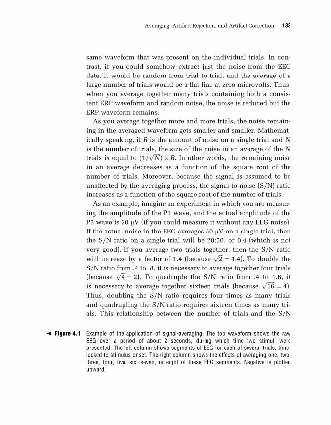
same waveform that was present on the individual trials. In con-
trast, if you could somehow extract just the noise from the EEG
data, it would be random from trial to trial, and the average of a
large number of trials would be a flat line at zero microvolts. Thus,
when you average together many trials containing both a consis-
tent ERP waveform and random noise, the noise is reduced but the
ERP waveform remains.
As you average together more and more trials, the noise remain-
ing in the averaged waveform gets smaller and smaller. Mathemat-
ically speaking, if R is the amount of noise on a single trial and N
is the number of trials, the size of the noise in an average of the N
trials is equal to ð1=ffiffiffiffiffi
Np
Þ R. In other words, the remaining noise
in an average decreases as a function of the square root of the
number of trials. Moreover, because the signal is assumed to be
unaffected by the averaging process, the signal-to-noise (S/N) ratio
increases as a function of the square root of the number of trials.
As an example, imagine an experiment in which you are measur-
ing the amplitude of the P3 wave, and the actual amplitude of the
P3 wave is 20 mV (if you could measure it without any EEG noise).
If the actual noise in the EEG averages 50 mV on a single trial, then
the S/N ratio on a single trial will be 20:50, or 0.4 (which is not
very good). If you average two trials together, then the S/N ratio
will increase by a factor of 1.4 (becauseffiffiffi
2p
¼ 1:4). To double the
S/N ratio from .4 to .8, it is necessary to average together four trials
(becauseffiffiffi
4p
¼ 2). To quadruple the S/N ratio from .4 to 1.6, it
is necessary to average together sixteen trials (becauseffiffiffiffiffiffi
16p
¼ 4).
Thus, doubling the S/N ratio requires four times as many trials
and quadrupling the S/N ratio requires sixteen times as many tri-
als. This relationship between the number of trials and the S/N
H Figure 4.1 Example of the application of signal-averaging. The top waveform shows the rawEEG over a period of about 2 seconds, during which time two stimuli werepresented. The left column shows segments of EEG for each of several trials, time-locked to stimulus onset. The right column shows the effects of averaging one, two,three, four, five, six, seven, or eight of these EEG segments. Negative is plottedupward.
Averaging, Artifact Rejection, and Artifact Correction 133

ratio is rather sobering, because it means that achieving a substan-
tial increase in S/N ratio requires a very large increase in the num-
ber of trials. This leads to a very important principle: It is usually
much easier to improve the quality of your data by decreasing
sources of noise than by increasing the number of trials.
To exemplify these principles, figure 4.1 shows the application
of signal averaging to a P3 oddball experiment. The top portion of
the figure shows the continuous EEG signal, from which the single-
trial EEG segments are taken. The left column shows the EEG seg-
ments for eight different trials in which an infrequent target was
presented. The P3 wave for this subject was quite large, and it can
be seen in every trial as a broad positivity in the 300–700 ms la-
tency range. However, there is also quite a bit of variability in the
exact shape of the P3 wave, and this is at least partly due to ran-
dom EEG fluctuations (the P3 itself may also vary from trial to
trial). The right column in figure 4.1 shows how averaging together
more and more trials minimizes the effects of the random EEG fluc-
tuations. The difference between trial 1 alone and the average of
trials 1 and 2 is quite substantial, whereas the difference between
the average of trials 1–7 and the average of trials 1–8 is small
(even though trial 8 is quite different from the other trials). Note
also that the S/N ratio in the average of trials 1–8 is 2.8 times
greater than the S/N ratio on the individual trials (becauseffiffiffi
8p
¼ 2:8).
The signal-averaging approach is based on several assumptions,
the most obvious of which are that (a) the neural activity related to
the time-locking event is the same on every trial, and (b) only the
EEG noise varies from trial to trial. These assumptions are clearly
unrealistic, but violations are not problematic in most cases. For
example, if the amplitude of the P2 wave varies from trial to trial,
then the P2 wave in the averaged ERP waveform will simply reflect
the average amplitude of the P2 wave. Similarly, one could imag-
ine that a P1 wave is present on some trials, a P2 wave is present
on other trials, and that both components are never present to-
gether on a given single trial. The averaged ERP waveform, how-
Chapter 4 134

ever, would contain both a P1 wave and a P2 wave, which would
incorrectly imply that the two components are part of the same
waveform. However, the conclusions of most ERP experiments do
not depend on the assumption that the different parts of the aver-
aged waveform are actually present together on individual trials,
so this sort of variability is not usually problematic as long as you
always remember that the average is only one possible measure of
central tendency.
The Problem of Latency Variability
Although trial-to-trial variability in ERP amplitude is not usually
problematic, trial-to-trial variability in latency is sometimes a sig-
nificant problem. Figure 4.2A illustrates this, showing four indi-
vidual trials in which a P3-like ERP component occurs at different
latencies. The peak amplitude of the average of these trials is much
smaller than the peak amplitude on the individual trials. This is
particularly problematic when the amount of latency variability
differs across experimental conditions. As figure 4.2B shows, a re-
duction in latency variability causes the peak amplitude of the av-
erage to be larger. Thus, if two experimental conditions or groups
of subjects differ in the amount of latency variability for some ERP
component, they may appear to differ in the amplitude of that com-
ponent even if the single-trial amplitudes are identical, and this
could lead an investigator to incorrectly conclude that there was a
difference in amplitude. Worse yet, latency variability can some-
times make it completely impossible to see a given neural response
in an averaged waveform (see figure 4.2C). For example, imagine a
sinusoidal oscillation that is triggered by a stimulus but varies ran-
domly in phase from trial to trial (which is not just a hypothetical
problem—see Gray et al., 1989). Such a response will average to
zero and will be essentially invisible in an averaged response.
Figure 4.3 shows a real-world example of latency jitter (from
Luck & Hillyard, 1990). In this experiment, we examined the P3
wave during two types of visual search tasks. In one condition
Averaging, Artifact Rejection, and Artifact Correction 135

Trial
1
Trial
2
Trial
3
Trial
4
Average
Average
Average
A
B
C
Trial
1Tr
ial 2
Trial
3
Trial
4
Trial
1
Trial
2
Trial
3
Trial
4
Chapter 4 136

(parallel search), subjects searched for a target with a distinctive
visual feature that ‘‘popped out’’ from the display and could be
detected immediately no matter how many distractor items were
present in the stimulus array. In the other condition (serial search),
the target was defined by the absence of a feature, and we expected
that in this condition the subjects would search one item at a
time until they found the target. In this condition, therefore, we
expected reaction time to increase as the number of items in the
array (the set size) was increased, whereas we expected no effect
of set size in the parallel search condition. This was the pattern of
results that we obtained.
We also predicted that both P3 latency and P3 amplitude would
increase at the larger set sizes in the serial search condition, but
not in the parallel search condition. However, because the order
in which the subjects search the arrays is essentially random, we
also predicted that there would be more trial-to-trial variability in
P3 latency at the larger set sizes in the serial search condition,
which made it difficult to measure P3 amplitude and latency. At
set size 4, for example, the target could be the first, second, third,
or fourth item searched, but at set size 12, the target might be
found anywhere between first item and the twelfth item. Conse-
quently, we predicted that P3 latency would be more variable at
the larger set sizes in the serial search condition (but not in the
parallel search condition, in which the target was detected imme-
diately regardless of the set size).
Figure 4.3B shows the averaged ERP waveforms from this exper-
iment. In the parallel search condition, the P3 wave was relatively
large in amplitude and short in duration, and it did not vary much
H Figure 4.2 Example of the problem of latency variation. Each panel shows four single-trialwaveforms, along with the average waveform. The same waveforms are present inpanels A and B, but there is greater latency variability in panel A than in panel B,leading to a smaller peak amplitude and broader temporal extent for the averagewaveform in panel A. Panel C shows that when the single-trial waveforms are notmonophasic, but instead have both positive and negative subcomponents, latencyvariability may lead to cancellation in the averaged waveform.
Averaging, Artifact Rejection, and Artifact Correction 137

500ms
-3 µV
+3 µV
Stimulus
Target = Target =
Stimulus
Response Response
Parallel Search
StimulusLocked
Averages
Stimuli
Serial Search
ResponseLocked
Averages
Set Size = 4Set Size = 8Set Size = 12
A
B
C
Figure 4.3 Example of an experiment in which significant latency variability was expected forthe P3 wave (Luck & Hillyard, 1990). (A) Sample stimuli from the two conditions ofthe experiment. (B) Stimulus-locked averages. (C) Response-locked averages. Nega-tive is plotted upward.
Chapter 4 138

as a function of set size. In the serial search condition, the P3 had a
smaller peak amplitude but was very broad. If you were to measure
the amplitude and latency at the peak of the P3 wave in the serial
search condition, you might conclude that set size didn’t have
much of an effect on the P3 in either the serial or parallel search
conditions. However, both the amplitude and the latency of the
P3 wave were significantly influenced by set size in the serial
search condition, although these effects were masked by the la-
tency variability.
I will now describe some techniques that you can use to mini-
mize the effects of latency variability.
Area Measures In most cases, you can mitigate the reduction in am-
plitude caused by latency variability simply by using an area am-
plitude measure rather than a peak amplitude measure. The area
under the curve in an average of several trials is always equal to
the average of the areas under the curves in each of the individual
trials, and an area measure will therefore be completely unaffected
by latency variability. In the experiment illustrated in figure 4.3,
for example, the area amplitude was significantly greater at larger
set sizes, even though peak amplitude was slightly smaller at the
larger set sizes. It is also possible to use an area-based measure of
latency rather than a peak-based measure. To do this, you simply
measure the area under the curve and find the time point that
divides this area into equal halves (this is called a 50 percent area
latency measure). When this measure was applied to the data
shown in figure 4.3B, the effects of set size on P3 latency were
found to be almost identical to the effects on reaction time. Chapter
6 will discuss these area-based measures in greater detail.
Area-based measures are almost always superior to peak-based
measures, and insensitivity to latency variability is just one of
several reasons why I prefer area-based measures. There are two
caveats, however. First, the equivalence between the area in the
individual trials and the area in the average is true only when the
Averaging, Artifact Rejection, and Artifact Correction 139

latency range used to measure the area spans the entire latency
range of the component. When there are multiple overlapping ERP
components that vary across conditions, it is sometimes necessary
to use a relatively restricted measurement window, in which case
the area measure is no longer completely insensitive to latency
variability (although it’s still usually better than a peak amplitude
measure). The second caveat is that area measures can misrepre-
sent components that are multiphasic (i.e., components with both
positive and negative portions). As figure 4.2C shows, the negative
and positive portions of a multiphasic waveform may cancel each
other when latency variability is present, and once the data have
been averaged there is no way to recover the information that is
lost due to this cancellation. Thus, area-based measures are useful
for mitigating the effects of latency variability under most condi-
tions, but they are not adequate when there is variability in a mul-
tiphasic waveform or when overlapping components preclude the
use of a wide measurement window.
Response-Locked Averages In some cases, variations in the latency
of an ERP component are correlated with changes in reaction time,
and in these cases latency variability can be corrected by using
response-locked averages rather than stimulus-locked averages. In
a response-locked average, the response rather than the stimulus
is used to align the single-trial EEG segments during the averaging
process. Consider, for example, the visual search experiment illus-
trated in figure 4.3. In the serial search condition, the P3 wave was
‘‘smeared out’’ by latency variability in the stimulus-locked aver-
ages, leading to a low peak amplitude and a broad waveform.
When response-locked averages were computed, however, the P3
wave in this condition was larger and much more narrowly peaked
(see figure 4.3C). In addition, the response-locked averages show
that the P3 wave was actually larger at set size 12 than at set size
4, even though the peak amplitude was larger for set size 4 in the
stimulus-locked averages. Many studies have used response-locked
averages in this manner.
Chapter 4 140

The Woody Filter Technique A third technique for mitigating the
effects of latency variability is the Woody filter technique (Woody,
1967). The basic approach of this technique is to estimate the la-
tency of the component of interest on individual trials and to use
this latency as the time-locking point for averaging. The compo-
nent is identified on single trials by finding the portion of the
single-trial waveform that most closely matches a template of the
ERP component. Of course, the success of this technique depends
on how well the component of interest can be identified on indi-
vidual trials, which in turn depends on the S/N ratio of the indi-
vidual trials and the similarity between the waveshape of the
component and the waveshape of the noise.
The Woody filter technique begins with a best-guess template of
the component of interest (such as a half cycle of a sine wave) and
uses cross-correlations to find the segment of the EEG waveform on
each trial that most closely matches the waveshape of the tem-
plate.1 The EEG epochs are then aligned with respect to the esti-
mated peak of the component and averaged together. The resulting
averaged ERP can then be used as the template for a second itera-
tion of the technique, and additional iterations are performed until
little change is observed from one iteration to the next.
The shortcoming of this technique is that the part of the wave-
form that most closely matches the template on a given trial may
not always be the actual component of interest, resulting in an
averaged waveform that does not accurately reflect the ampli-
tude and latency of the component of interest (see Wastell, 1977).
Moreover, this does not simply add random noise to the averages;
instead, it tends to make the averages from each different experi-
mental condition more similar to the template and therefore more
similar to each other (this is basically just regression toward the
mean). Thus, this technique is useful only when the component of
interest is relatively large and dissimilar to the EEG noise. For ex-
ample, the P1 wave is small and is similar in shape to spontaneous
alpha waves in the EEG, and the template would be more closely
matched by the noise than by the actual single-trial P1 wave on
Averaging, Artifact Rejection, and Artifact Correction 141

many trials. The P3 component, in contrast, is relatively large
and differs in waveshape from common EEG patterns, and the
template-matching procedure is therefore more likely to find the
actual P3 wave on single trials.
However, even when one is examining a large component such
as the P3 wave, Woody filtering works best when the latency vari-
ability is only moderate; when the variability is great, a very wide
window must be searched on the individual trials, leading to more
opportunities for a noise deflection to match the template better
than the component of interest. For example, I tried to apply the
Woody filter technique to the visual search experiment shown in
figure 4.3, but it didn’t work very well. The P3 wave in this experi-
ment could peak anywhere between 400 and 1,400 milliseconds
poststimulus, and given this broad search window, the algorithm
frequently located a portion of the waveform that matched the
search template fairly well but did not correspond to the actual P3
peak. As a result, the averages looked very much like the search
template and were highly similar across conditions.
One should note that the major difficulty with the Woody filter
technique lies in identifying the component of interest on single
trials, and any factors that improve this process will lead to a
more accurate adjustment of the averages. For example, the scalp
distribution of the component could be specified in addition to the
component’s waveshape, which would make it possible to reject
spurious EEG deflections that may have the correct waveshape but
have an incorrect scalp distribution (see Brandeis et al., 1992).
Time-Locked Spectral Averaging The final technique considered here
is a means of extracting oscillatory responses that have random
phase (onset time) with respect to the time-locking event. As dis-
cussed at the beginning of this section, oscillations that vary in
phase will be lost in a conventional average, but one can see these
oscillations using techniques that measure the amplitudes of the
oscillations on single trials and then average these amplitude
measures across trials. The techniques for measuring single-trial
Chapter 4 142

oscillation amplitudes rely on variants of a mathematical proce-
dure called the Fourier transform. As I will discuss more fully in
chapter 5, the Fourier transform converts a waveform into a set of
sine waves of different frequencies, phases, and amplitudes. For
example, if you were to apply the Fourier transform to a 1-second
EEG epoch, you would be able to determine the amount of activity
at 10 Hz, at 15 Hz, at 20 Hz, or almost any frequency. In this man-
ner, you could compute the amplitude at each frequency for a
single trial, and you could then average these amplitude measures
across trials. Moreover, because the amplitude is measured inde-
pendently of the phase, it wouldn’t matter if the phase (i.e., the la-
tency) of the oscillations varied across trials.
Although this is a useful approach, it completely discards the
temporal information of the ERP technique, because the amplitude
measured on a given trial is the amplitude for the entire time
period. Temporal information can be retained, however, by using
moving window techniques, such as those developed by Makeig
(1993) and by Tallon-Baudry and colleagues (1996). These techni-
ques extract a brief window of EEG from the beginning of the trial
(e.g., the first 100 ms of EEG). The Fourier transform is then ap-
plied to this window to provide a quantification of the amplitude
at each frequency during that relatively brief time range. The
window is then moved over slightly (e.g., by 10 ms), and another
Fourier transform is applied. In this manner, it is possible to com-
pute Fourier transforms for every point in the EEG, although the
values at a given time point actually represent the frequencies
over a period of time (e.g., a 100-ms period). The Fourier trans-
forms at a given time point are then averaged across trials just
as the EEG amplitude would be averaged across trials in a con-
ventional average. This is called time-locked spectral averaging
because time-locked averages are computed for spectral (i.e., fre-
quency) information.
Figure 4.4A2 shows an example of this technique, presenting
time-locked spectral averages from the study of Tallon-Baudry et
al. (1996), who were interested in the 40-Hz oscillations elicited
Averaging, Artifact Rejection, and Artifact Correction 143

by visual stimuli. The X-axis in this plot is time, just as in a tradi-
tional ERP average. The Y-axis, however, is frequency, and the
gray-scale level indicates the power that was present at each fre-
quency at each time point. A band of activity between 40 and 50
Hz can be seen at approximately 100 ms poststimulus, and a some-
what weaker band of activity between 30 and 60 Hz can be seen at
approximately 300 ms poststimulus. Activity can also be seen in
the 20-Hz range from about 100 to 200 ms poststimulus.
The crucial aspect of this approach is that these bands of activity
can be seen whether or not the oscillations vary in phase from trial
to trial, whereas random-phase activity is completely lost in a tra-
ditional average. Time-locked spectral averaging thus provides a
very useful technique for examining random-phase oscillations.
However, it is very easy to draw an incorrect conclusion from data
such as those shown in figure 4.4A, namely that the activity really
consists of oscillations. As I will discuss fully in chapter 5, a brief
A) Time X Frequency Activity onSingle Trials
B) Time X Frequency Activity fromAveraged ERPs
100Hz
80
60
40
20
100Hz
80
60
40
20–200 –100 0 100 200 300 400 ms –200 –100 0 100 200 300 400 ms
Figure 4.4 Example of time-locked spectral averaging. In panel A, the frequency transformationwas applied to the individual trials and the transformed data were then averaged.This plot therefore includes activity that was not phase-locked to stimulus onset aswell as phase-locked activity. In panel B, the transformation was applied after thewaveforms had been averaged together. This plot therefore includes only activitythat was phase-locked to the stimulus, because random-phase activity is eliminatedby the ERP averaging process. (Adapted with permission from Tallon-Baudry et al.,1996. > 1996 Society for Neuroscience.)
Chapter 4 144

monophasic ERP deflection contains activity at a variety of fre-
quencies, and the presence of activity in a given frequency band
does not entail the existence of a true oscillation (i.e., an oscilla-
tion with multiple positive and negative deflections). For example,
figure 4.4B shows the time frequency transformation of the tradi-
tional ERP averages from the study of Tallon-Baudry et al. (1996),
and the 40–50 Hz activity at 100 ms poststimulus can be seen in
this plot just as in the single-trial data. In other words, this activity
was a part of the traditional ERP and was not a random-phase os-
cillation. Thus, to draw conclusions about random-phase oscilla-
tions, it is necessary to apply the time frequency transformation
to the averaged ERPs as well as to the single-trial EEG data.
Overlap from Preceding and Subsequent Stimuli
Overlapping ERPs from previous and subsequent stimuli will dis-
tort averaged ERP waveforms in ways that are sometimes subtle
and sometimes obvious, and it is important to understand how
this arises and when it might lead you to misinterpret your data
(for a detailed treatment of this issue, see Woldorff, 1988). Overlap
arises when the response to the previous stimulus has not ended
before the baseline period prior to the current stimulus or when
the subsequent stimulus is presented before the ERP response to
the current stimulus has terminated. This problem is particularly
acute when stimuli are presented rapidly (e.g., 1 second or less
between stimulus onsets). However, ERP waveforms can last for
several seconds, and overlap can significantly distort your data
even at long interstimulus intervals.
Figure 4.5 illustrates the overlap problem for a thought experi-
ment in which a stimulus is presented every 300–500 ms. Panel A
shows the actual waveform elicited by a given stimulus without
any overlap. Note that the prestimulus period is flat and that the
waveform falls to zero at 1000 ms poststimulus. Panel B shows
the waveforms that the same stimulus would have produced if
Averaging, Artifact Rejection, and Artifact Correction 145
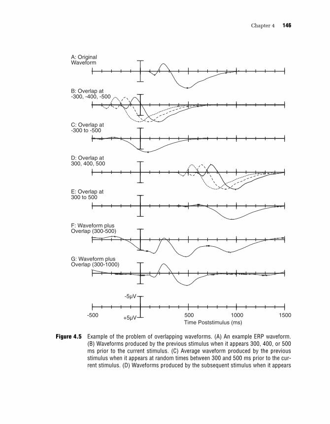
A: OriginalWaveform
-5µV
+5µV-500 500 1000 1500Time Poststimulus (ms)
B: Overlap at-300, -400, -500
C: Overlap at-300 to -500
E: Overlap at300 to 500
D: Overlap at300, 400, 500
F: Waveform plusOverlap (300-500)
G: Waveform plusOverlap (300-1000)
Figure 4.5 Example of the problem of overlapping waveforms. (A) An example ERP waveform.(B) Waveforms produced by the previous stimulus when it appears 300, 400, or 500ms prior to the current stimulus. (C) Average waveform produced by the previousstimulus when it appears at random times between 300 and 500 ms prior to the cur-rent stimulus. (D) Waveforms produced by the subsequent stimulus when it appears
Chapter 4 146

it appeared 300, 400, or 500 ms prior to the current stimulus;
these are just the original waveform shifted to the left by various
amounts. Panel C shows the average of a large number of previous
waveforms, elicited by stimuli happening randomly and equiprob-
ably between 300 and 500 ms prior to the current stimulus. This is
the average overlap from the preceding stimuli. Panel D shows the
responses elicited by the subsequent stimulus at 300, 400, or 500
ms, and panel E shows the overlap that would occur with stimuli
occurring randomly 300–500 ms after the current stimulus.
Note that the jittered timing in this thought experiment leads to a
‘‘smearing’’ of the averaged waveform for the overlapping stimuli.
That is, the relatively sharp positive and negative peaks at the be-
ginning of the original waveform are mostly (but not entirely) elim-
inated in the overlapping waveform. The effect of temporal jitter
between stimuli is equivalent to filtering out the high frequencies
from the original waveform. As the range of time delays between
the stimuli becomes wider and wider, the jitter reduces lower and
lower frequencies from the overlap. However, even with a broad
jitter, some low-frequency overlap will still occur (chapter 5 will
describe a set of mathematical formalizations that you can use to
understand in detail the filtering properties of temporal jitter).
Panel F shows the sum of the original waveform and the overlap-
ping waveforms. This sum is exactly what you would obtain if you
simply averaged together all of the stimuli in this thought experi-
ment. The distortion due to overlap is quite severe. First, the pres-
timulus baseline is completely distorted, and this leads the initial
positive component to seem much larger than it really is (compare
the first positive component in panel G to the original waveform
H Figure 4.5 (continued)300, 400, or 500 ms after the current stimulus. (E) Average waveform produced bythe subsequent stimulus when it appears at random times between 300 and 500 msafter the current stimulus. (F) Sum of the original waveform and the overlappingwaveforms from (C) and (E). (G) Sum of the original waveform and the overlappingwaveforms that would be produced if the interval between stimuli was increased to300–1000 ms. Negative is plotted upward.
Averaging, Artifact Rejection, and Artifact Correction 147

in panel A). Second, the first positive component appears to start
before time zero (which is always a good indication that something
is amiss). Third, there is a late positive peak that is completely
artifactual.
Overlap is particularly problematic when it differs between ex-
perimental conditions. Imagine, for example, that the same target
stimulus is presented in condition A and in condition B, and the
preceding stimulus elicits a large P3 wave in condition A and a
small P3 wave in condition B. This difference in the preceding
stimuli may influence the prestimulus baseline period, and this in
turn will influence the apparent amplitude of the P3 elicited by the
target stimuli on the current trial. Note that this can happen even
if the ERP response to the preceding stimulus has returned to
baseline before the P3 wave on the current trial: if the baseline is
affected, then the whole waveform will be affected. This can also
have a big impact on attempts to localize the generator of an
ERP component, because the scalp distribution of the overlapping
activity in the prestimulus period will be subtracted away from
the scalp distribution of the component that you are trying to local-
ize, distorting the apparent scalp distribution of the component.
There are some steps that you can take to minimize the effects
of overlap. The first and most important step is to think carefully
about exactly what pattern the overlap will take and how it might
differ across conditions (for an example, see Woldorff & Hillyard,
1991). The key is to think about how the task instructions may
change the response to the preceding stimulus across conditions,
even if it is the same physical stimulus. You may even want to sim-
ulate the overlap, which isn’t conceptually difficult (for details, see
Woldorff, 1988). It’s computationally trivial to do this in a pro-
gramming environment such as MATLAB, and it can even be done
fairly easily in Excel.
A second approach is to use the broadest possible range of time
delays between stimuli. Panel G of figure 4.5 shows what happens
if the jitter in our thought experiment is expanded to 300–1000 ms.
There is still some overlap, but it is much smaller.
Chapter 4 148

A third approach is to use high-pass filters to filter out any
remaining overlap. As mentioned earlier in this section, jittering
the interstimulus interval is equivalent to filtering out the high fre-
quencies from the overlap, and the remaining low frequencies can
be filtered offline with a high-pass filter. High-pass filtering can dis-
tort your waveforms in other ways, however, so you must do this
cautiously (see chapter 5 for details).
A fourth approach is to design the experiment in a way that
allows you to directly measure and subtract away the overlap. In
our thought experiment, for example, we could include occasional
trials on which no stimulus was presented and create averaged
waveforms time-locked to the time at which the stimulus would
ordinarily have occurred. These waveforms will contain only the
overlap, and these overlap waveforms can be subtracted from the
averaged waveforms that contained the response to an actual stim-
ulus along with the overlap. This requires some careful thought,
however, because the subject might notice the omission of a stim-
ulus triggering an ERP (see, e.g., Picton, Hillyard, & Galambos,
1974). I have frequently used this approach in my own research
(see, in particular, Luck, 1998b; Vogel, Luck, & Shapiro, 1998).
A fifth approach is to estimate the overlap from the data you
have collected and subtract the estimated overlap from the aver-
aged ERP waveforms. Woldorff (1988) has developed a technique
called the ADJAR (adjacent response) filter that has been used
for this purpose in a number of experiments (e.g., Hopfinger &
Mangun, 1998; Luck et al., 1994; Woldorff & Hillyard, 1991).
Transient and Steady-State ERPs
If stimuli are presented at a constant rate rather than a variable
rate, the overlap from the preceding and subsequent stimuli is fully
present in the averaged ERP waveforms. In fact, the preceding and
subsequent stimuli are perfectly time-locked to the current stimu-
lus, so it makes sense that they would appear in the averaged ERP
waveforms. Most cognitive ERP experiments therefore use some
Averaging, Artifact Rejection, and Artifact Correction 149

jitter in the interstimulus interval unless the interstimulus interval
is fairly long.
It is sometimes possible to make overlap into a virtue. Specifi-
cally, if a series of identical stimuli are presented at a fast, regular
rate (e.g., eight stimuli per second), the system will stop producing
complex transient responses and enter into a steady state, in which
the system resonates at the stimulus rate (and multiples thereof).
Typically, steady state responses will look like two summed sine
waves, one at the stimulation frequency and one at twice the stim-
ulation frequency.
Figure 4.6 shows an example of a steady state response. The up-
per left portion of the figure shows the transient response obtained
when the on-off cycle of a visual stimulus repeats twice per sec-
ond. When the stimulation rate is increased to 6 cycles per second,
it is still possible to see some distinct peaks, but the overall wave-
form now appears to repeat continuously, with no clear beginning
or end. As the stimulation rate is increased to 12 and then 20
0 50 100 150 200 250
C1
P1
N1
0 50 100 150 200 250
0 50 100 150 200 250 0 50 100 150 200 250
Time (ms)
2 Hz 6 Hz
12 Hz 20 Hz
Am
plitu
de (
µV
)
Figure 4.6 Transient response to a stimulus presented at a rate of two on-off cycles per secondand steady-state response to a stimulus presented at 6, 12, or 20 Hz. Positive isplotted upward. (Adapted with permission from Di Russo, Teder-Salejarvi, & Hill-yard, 2003. > 2003 Academic Press.) Thanks to Francesco Di Russo for providingan electronic version of this figure.
Chapter 4 150

cycles per second, the response is predominantly a sine wave at
the stimulation frequency (with a small, hard-to-see component at
twice the stimulation frequency).
This steady-state response can be summarized by four numbers,
the amplitude (size) and phase (temporal shift) of each of the two
sine waves. This is a lot simpler than a complex transient response
with a separate amplitude value at each point in time. As a result,
steady-state ERPs are widely used in the study of sensory systems
and in the diagnosis of sensory disorders.
Steady-state ERPs have a significant shortcoming, however,
which is that they do not provide very precise temporal informa-
tion. For example, if stimuli are presented every 150 ms, the volt-
age measured at 130 ms after the onset of one stimulus consists
of the sum of the response to the current stimulus at 130 ms, the
response to the previous stimulus at 280 ms, the response to the
stimulus before that at 430 ms, and so on. Because steady-state
ERPs lack the high temporal resolution of transient ERPs, they are
used only rarely in cognitive studies (for a review of some recent
cognitive steady-state studies, see Hopfinger, Luck, & Hillyard,
2004).
Artifact Rejection and Correction
Now that we have considered the averaging process, we will move
on to the artifact rejection procedures that typically accompany it.
There are several types of artifacts that can contaminate EEG
recordings, including blinks, eye movements, muscle activity, and
skin potentials. These artifacts can be problematic in two ways.
First, they are typically very large compared to the ERP signals
and may greatly decrease the S/N ratio of the averaged ERP wave-
form. Second, some types of artifacts may be systematic rather than
random, occurring in some conditions more than others and being
at least loosely time-locked to the stimulus so that the averaging
process does not eliminate them. Such artifacts may lead to errone-
ous conclusions about the effects of an experimental manipulation.
Averaging, Artifact Rejection, and Artifact Correction 151

For example, some stimuli may be more likely to elicit blinks than
others, which could lead to differences in amplitude in the aver-
aged ERP waveforms.
There are two main classes of techniques for eliminating the
deleterious effects of artifacts. First, it is possible to detect large
artifacts in the single-trial EEG epochs and simply exclude conta-
minated trials from the averaged ERP waveforms (this is called ar-
tifact rejection). Alternatively, it is sometimes possible to estimate
the influence of the artifacts on the ERPs and use correction proce-
dures to subtract away the estimated contribution of the artifacts
(this is called artifact correction). In this section, I will discuss
both approaches. However, I would first like to make a point that
should be obvious but is often overlooked. Specifically, it is always
better to minimize the occurrence of artifacts rather than to rely
heavily on rejection or correction procedures. This is really just a
special case of Hansen’s Axiom: there is no substitute for good
data. In other words, time spent eliminating artifacts at the source
will be well rewarded. This section will therefore also include
hints for reducing the occurrence of artifacts.
The General Artifact Rejection Process
Before I get into the details of how to detect specific types of arti-
facts, I would like to provide a general framework for conceptualiz-
ing the artifact rejection process.3 Detecting artifacts is, in essence,
a signal detection problem, in which the artifact is treated as the
to-be-detected signal. As an example, imagine that you have lost a
valuable ring on a beach, and you have rented a metal detector to
help you find it. The metal detector has a continuously variable
output that tells you the extent to which there is evidence of
nearby metal, but this output is quite variable due to random fluc-
tuations in the mineral content of the sand. If you started digging
in the sand any time there was a hint of nearby metal, you would
make very slow progress because you would start digging every
few feet. However, if you only started digging when the metal
Chapter 4 152

detector’s output was very high, you might miss the ring altogether
because it is small and doesn’t create a large change in the detec-
tor’s output. Thus, if you dig only when the detector’s output
reaches a very high level, you will probably pass right over the top
of the ring, but if you dig whenever the output exceeds some small
level, you will frequently be digging in vain.
The key aspects of this example are as follows. You are trying to
detect something that is either there or not (the ring) based on a
noisy, continuously variable signal (the metal detector’s output).
You select a threshold value, and if the signal exceeds that value,
you make a response (digging). In this context, we can define four
outcomes for each patch of sand: (1) a hit occurs when the sought-
after object is present, the signal exceeds the threshold, and you re-
spond (i.e., the metal detector’s output exceeds a certain value, you
dig, and you find the ring); (2) a miss occurs when the object is
present, the signal fails to exceed the threshold, and you don’t re-
spond; (3) a false alarm occurs when the object is absent, the signal
exceeds the threshold due to random variation, and you respond;
(4) a correct rejection occurs when the object is absent, the signal
doesn’t exceed the threshold, and you don’t respond. Hits and cor-
rect rejections are both correct responses, and misses and false
alarms are both errors. Importantly, you can increase the number
of hits by choosing a lower threshold (i.e., digging when the metal
detector’s output is fairly low), but this will also lead to an increase
in the number of false alarms. The only way to increase the hit rate
without increasing the false alarm rate is to get a better metal de-
tector with an output that better differentiates between the pres-
ence or absence of small metal objects.
Now imagine that you are trying to detect blinks in a noisy EEG
signal. When a subject blinks, the movement of the eyelids across
the eyeball creates a voltage deflection, and it is possible to assess
the presence or absence of a blink by measuring the size of the
largest voltage deflection within a given segment of EEG (just like
assessing the presence or absence of the ring by examining the
output of the metal detector). If the voltage deflection exceeds a
Averaging, Artifact Rejection, and Artifact Correction 153

certain threshold level, you conclude that the subject blinked and
you discard that trial; if the threshold is not exceeded, you con-
clude that the subject did not blink and you include that trial in
the averaged ERP waveform. If you set a low threshold and reject
any trials that have even a small voltage deflection, you will elimi-
nate all of the trials with blinks, but you will also discard many
blink-free trials, reducing the signal-to-noise ratio of the averaged
ERP waveform. If you set a high threshold and reject only trials
with very large voltage deflections, you will have more trials in
your averages, but some of those trials may contain blinks that
failed to exceed your threshold. Thus, simply changing the thresh-
old cannot increase the rejection of true artifacts without also
increasing the rejection of artifact-free trials. However, just as you
can do a better job of finding a ring in the sand by using a better
metal detector, you can do a better job of rejecting artifacts by us-
ing a better procedure for measuring artifacts.
Choosing an Artifact Measure
Many software systems assess blinks by measuring the maximal
voltage in the EOG signal on a given trial and rejecting trials in
which this maximal voltage exceeds a threshold, such as G75 mV.
However, the peak amplitude in the EOG channel is a very poor
measure of blink artifacts, because variations in the baseline volt-
age can bring the EOG signal far enough away from zero that small
noise deflections will sometimes cause the voltage to exceed the
threshold voltage, causing false alarms. Variations in baseline volt-
age can also bring the EOG signal away from the threshold voltage
so that a true blink no longer exceeds the threshold, leading to
misses.
Figure 4.7 illustrates these problems. Panel A of the figure
shows an EOG recording with a blink that exceeds the 75 mV
threshold and would be correctly rejected. Panel B shows an epoch
in which a blink is clearly present, but because the baseline has
shifted, the 75 mV threshold is not exceeded (a miss). Panel C
Chapter 4 154

shows an epoch in which no blink was present, but a shift in base-
line causes the 75 mV threshold to be exceeded by simple noise (a
false alarm).
An alternative approach is to measure the difference between the
minimum and maximum voltages within an EOG epoch and to
compare this peak-to-peak voltage with some threshold voltage.
This peak-to-peak measure is less distorted by slow changes in
baseline voltage, reducing the impact of this possible source of
misses and false alarms, and increasing the sensitivity of the arti-
fact rejection process. Thus, it is possible to increase the rejec-
tion of trials with artifacts without increasing the rejection of
–75 µV
–75 µV
–75 µV
+75 µV
+75 µV
+75 µV
A
B
C
Figure 4.7 Example of the use of an absolute voltage threshold for artifact rejection. Eachwaveform shows single-trial activity recorded from an EOG electrode under the lefteye, with a right-mastoid reference. In panel A, a blink is present and exceeds thethreshold. In panel B, a blink is again present, but because the voltage had drifteddownward, the threshold is not exceeded. In panel C, no blink is present, butbecause of a downward drift in the signal, the threshold is exceeded. Negative isplotted upward.
Averaging, Artifact Rejection, and Artifact Correction 155

artifact-free trials by choosing a measure that can accurately distin-
guish between trials with and without artifacts. Later in this chap-
ter I’ll offer some suggestions for good measures.
The choice of the most sensitive measure will depend on what
type of artifact you are measuring. For example, although peak-to-
peak amplitude is a sensitive measure of blinks, it is not a very
sensitive measure of the presence of alpha waves, which are fre-
quently no larger than the background EEG activity. A more sensi-
tive measure of alpha waves would be, for example, the amount of
power in the 10-Hz frequency range, which would be high on trials
contaminated by alpha waves and low for uncontaminated trials.
Thus, a good artifact rejection system should allow the use of dif-
ferent measures for different types of artifacts.
It is important to note that a measure such as peak-to-peak am-
plitude is not really a measure of blinking, but is simply a numeric
value that you can calculate from the data and use to differentiate
probabilistically between trials with and without blinks. The arti-
fact rejection process can thus be conceptualized in the general
case as a two-step process, in which a ‘‘function’’ is applied to the
data to compute a specific value and then this value is compared to
the threshold. You can use different functions and different criteria
in different cases, depending on the nature of the artifact that you
are trying to detect.
Some investigators visually inspect the EEG on each trial to de-
termine which trials contain artifacts, but this process is concep-
tually identical to the procedure that I just outlined. The only
difference is that it uses the experimenter’s visual system instead
of a computer algorithm to determine the extent to which an arti-
fact appears to be present and uses an informal, internal threshold
to determine which trials to reject. The advantage of this approach
is that the human visual system can be trained to do an excellent
job of differentiating between real artifacts and normal EEG noise.
However, a well-designed computer algorithm may be just as sen-
sitive, if not more so. And computer algorithms have the advan-
tages of being fast and not being prone to bias. Thus, it is usually
Chapter 4 156

best to use a good automated artifact rejection system rather than
spending hours trying to identify artifacts by eye.
Choosing a Rejection Threshold
Once you have chosen an appropriate measure of an artifact, you
must choose the threshold that will be used to determine whether
to reject an individual trial. One possibility is to pick a threshold
on the basis of experience and use this value for all subjects. For
example, you may decide to reject all trials with a peak-to-peak
EOG amplitude of 50 mV or higher. However, there is often signifi-
cant variability across subjects in the size and shape of the voltage
deflections a given type of artifact produces and in the characteris-
tics of the EEG in which these voltage deflections are embedded, so
a one-size-fits-all approach is therefore not optimal. Instead, it is
usually best to tailor the artifact rejection process for each individ-
ual subject.
There is at least one exception to this rule, however: experiments
that use different subject groups and in which the artifact rejection
process could lead to some sort of bias. For example, it might not
be appropriate to use different artifact rejection criteria for different
subjects in a study that compared schizophrenia patients with nor-
mal controls, because any differences in the resulting averaged ERP
waveforms could reflect a difference in artifact rejection rather
than a real difference in the ERPs. However, using the same criteria
for all subjects could also be problematic in such a study if, for
example, one group had smaller blink amplitudes than another,
resulting in more contamination from artifacts that escaped rejec-
tion. The best compromise in between-subject studies is probably
to set the criteria individually for each subject, but to be blind to
the subject’s condition when the criteria are set. In addition, it
would be worthwhile to determine whether the results are any dif-
ferent when using the same threshold for all subjects compared to
when tailoring the threshold for each subject—if the results are the
same, then the threshold is not causing any bias in the results.
Averaging, Artifact Rejection, and Artifact Correction 157

If the threshold is set individually for each subject, the settings
are usually based on visual inspection of a portion of the raw EEG.
This can be accomplished by the following sequence of steps. First,
select an initial threshold for a given subject as a starting point
(usually on the basis of experience with prior subjects). Then
apply this threshold to a set of individual trials and visually assess
whether trials with real artifacts are not being rejected or if trials
without real artifacts are being rejected. Of course, this requires
that you are able to determine the presence or absence of artifacts
by visual inspection. In most cases, this is fairly straightforward,
and the next section provides some hints. After the initial thresh-
old has been tested on some data, it can be adjusted and retested
until it rejects all of the trials that clearly have artifacts without
rejecting too many artifact-free trials (as assessed visually). Some
types of artifacts also leave a distinctive ‘‘signature’’ in the aver-
aged waveforms, so it is also possible to evaluate whether the
threshold adequately rejected trials with artifacts after you have
averaged the data.
It can also be useful to ask the subject to make some blinks and
eye movements at the beginning of the session so that you can eas-
ily see what that subject’s artifacts look like.
Detecting and Rejecting Specific Types of Artifacts
In this section, I will discuss several common types of artifacts and
provide suggestions for reducing their occurrence and for detecting
and rejecting them when they do occur.
Blinks Within each eye, there is an electrical gradient with posi-
tive at the front of the eye and negative at the back of the eye, and
the voltage deflections recorded near the eye are primarily caused
by the movement of the eyelids across the eyes, which modulates
the conduction of the electrical potentials of the eyes to the sur-
rounding regions. Figure 4.8 shows the typical waveshape of the
eyeblink response at a location below the eyes (labeled VEOG) and
Chapter 4 158

at several locations on the scalp (all are referenced to a mastoid
electrode). The eyeblink response consists primarily of a monopha-
sic deflection of 50–100 mV with a typical duration of 200–400 ms.
Perhaps the most important characteristic of the eyeblink response,
however, is that it is opposite in polarity for sites above versus be-
low the eye (compare, for example, the VEOG and Fz recordings in
figure 4.8). This makes it possible to distinguish between a blink,
which would produce opposite-polarity voltage shifts above versus
below the eye, and a true EEG deflection, which would typically
produce same-polarity voltage shifts above and below the eye. The
-50 µV
200ms
1200ms
400ms
1400ms
600ms
1600ms
800ms
1800ms
1000ms
2000ms
+50 µV
VEOG
Fz
Cz
Pz
BlinkNot aBlink
Figure 4.8 Recordings from a vertical EOG (VEOG) electrode located under the left eye and EEGelectrodes located at Fz, Cz, and Pz, with a right mastoid reference for all record-ings. A blink can be seen at approximately 400 ms, and it appears as a negative de-flection at the VEOG electrode and as a positive deflection at the scalp electrodes.Note that the deflection is quite large at Fz and then becomes smaller at Cz andeven smaller at Pz. The area labeled ‘‘Not a Blink’’ contains moderately large voltagedeflections in all of these channels, but these deflections do not reflect a blinkbecause the polarity is not inverted at the VEOG electrode relative to the scalp elec-trodes. Negative is plotted upward.
Averaging, Artifact Rejection, and Artifact Correction 159

right side of figure 4.8 shows an example of a true EEG deflection,
where similar-polarity deflections appear at the VEOG and Fz sites.
Because of the polarity reversal exhibited by blinks, you should
always be suspicious of an experimental effect that is opposite in
polarity at electrode sites above versus below the eyes. Although
such a pattern is possible for a true ERP effect, it should serve as a
warning signal indicating that the averaged ERP waveforms may be
more contaminated by blinks in one condition than in the other.
Reducing the occurrence of an artifact is always better than
rejecting trials with artifacts, and there are several ways to reduce
the number of blinks. The first is to ask subjects who normally
wear contact lenses—which cause a great deal of blinking—to
wear their glasses instead of their contact lenses. These individuals
tend to blink more than average even when wearing glasses, and it
is therefore useful to keep a supply of eyedrops handy (although
you should offer them only to individuals who normally use eye-
drops, and you should use single-use bottles to avoid infection
risks). Another method for reducing the occurrence of blinks is to
use short trial blocks of 1–2 minutes, thus providing the subjects
with frequent rest breaks for blinking (this also helps to keep the
subjects more alert and focused on the task). The use of such
short trial blocks tends to slow down the progress of a record-
ing session, but I have found that this slowing can be mitigated
by using trial blocks of 5–6 minutes that are subdivided into
‘‘miniblocks’’ of 1–2 minutes, with automatic breaks of 20–30 sec-
onds interposed between the miniblocks and somewhat longer,
experimenter-controlled breaks between the full blocks.
If you see a lot of blinks (or eye movements), it is important to let
the subject know. Don’t be shy about telling subjects that they need
to do a better job of controlling these artifacts. My students tell me
that it took them a long time to become comfortable doing this, but
you really need to do it, even if it makes you uncomfortable at first.
Blinks are relatively easy to detect on single trials, and a peak-to-
peak amplitude measure is usually an adequate artifact rejection
function (a simple voltage threshold, however, is clearly inade-
Chapter 4 160

quate, because a threshold that is sufficiently low to reject all
blinks often leads to a large number of false alarms). The peak-
to-peak amplitude function can sometimes be ‘‘fooled’’ by slow
voltage shifts that cause one end of the epoch to be substantially
different in voltage from the other end, and high-frequency noise
(e.g., muscle activity) can exacerbate this. Both of these problems
can be minimized by a measure that I call a ‘‘step’’ function, which
basically looks for step-like changes in voltage. This function is
similar to performing a cross-correlation between the EEG/EOG
epoch and a function that looks like a step (i.e., a flat low interval
followed by a flat high interval). One first defines the width of the
step, with a typical value of 100 ms. For each point in the epoch,
the mean value of the preceding 100 ms is then subtracted from
the mean value of the subsequent 100 ms (or whatever the desired
step width is). After this has been computed for each point in the
epoch, the largest value is compared with the threshold to deter-
mine whether the trial should be rejected. This computationally
simple procedure is effective for two reasons. First, averaging to-
gether the voltage of a 100-ms interval essentially filters out any
high-frequency activity. Second, computing the difference between
successive 100-ms intervals minimizes the effects of any gradual
changes in voltage, which corresponds with the fact that a blink
produces a relatively sudden voltage change.
Whenever possible, one should obtain recordings from an elec-
trode below the eye and an electrode above the eye, with both elec-
trodes referenced to a common, distant site (e.g., an EOG electrode
located below one of the two eyes and a frontal EEG site, both
referenced to a mastoid electrode). This makes it possible to take
advantage of the inversion of polarity exhibited by blinks for
sites above and below the eyes, which is especially useful when
inspecting the single-trial data during the assessment of the ade-
quacy of the artifact rejection function and the threshold. As dis-
cussed above, this also makes it possible to determine whether the
ERP averages are contaminated by blinks, which leads to an inver-
sion in polarity for sites above versus below the eyes. In addition,
Averaging, Artifact Rejection, and Artifact Correction 161

this montage makes it possible to implement an even more power-
ful artifact rejection function, which I call the ‘‘differential step’’
function. This function is just like the step function, except that
one computes values at each time point for a location below and a
location above the eyes and then subtracts these two values from
each other. The maximum value of this difference is then com-
pared with a threshold to determine whether a given trial should
be rejected. The subtraction process ensures that a large value is
obtained only when the voltage is changing in opposite directions
for the electrodes above and below the eyes. A simpler but nearly
equivalent alternative is to apply the standard step function to a
bipolar recording in which the electrode beneath the eye is the
active site and the electrode above the eye is the reference.
Eye Movements Like blinks, eye movements are a result of the in-
trinsic voltage gradient of the eye, which can be thought of as a
dipole with its positive end pointing toward the front of the eye.
When the eyes are stationary, this dipole creates a constant DC
voltage gradient across the scalp, which the high-pass filter of the
amplifier eliminates. When the eyes move, the voltage gradient
across the scalp changes, becoming more positive at sites that the
eyes have moved toward. For example, a leftward eye movement
causes a positive-going voltage deflection on the left side of the
scalp and a negative-going voltage on the right side of the scalp. It
is easiest to observe these deflections with bipolar recordings, in
which an electrode lateral to one eye is the active site and an elec-
trode lateral to the other eye is the reference site.
Hillyard and Galambos (1970) and Lins et al. (1993a) have sys-
tematically measured the average size of the saccade-produced
deflection. These studies yielded the following findings: (a) the
voltage deflection at a given electrode site is a linear function of
the size of the eye movement, at least over a 15-degree range of
eye movements; (b) a bipolar recording of the voltage between elec-
trodes at locations immediately adjacent to the two eyes will yield
a deflection of approximately 16 mV for each degree of eye move-
Chapter 4 162

ment; and (c) the voltage falls off in a predictable manner as the
distance between the electrode site and the eyes increases (see
tables V and VI of Lins et al., 1993, for a list of the propagation fac-
tors for a variety of standard electrode sites).
Note also that eye movements cause the visual input to shift
across the retina, which creates a visual ERP response (saccadic
suppression mechanisms make us unaware of this motion, but
it does create substantial activity within the visual system). This
saccade-induced ERP depends on the nature of the stimuli that are
visible when the eyes move, just as the ERP elicited by a moving
stimulus varies as a function of the nature of the stimulus. Proce-
dures that attempt to correct for the EOG voltages produced by eye
movements—discussed at the end of this chapter—cannot correct
for these saccade-induced ERP responses.
Unless the subject is viewing moving objects or exhibiting grad-
ual head movements, the vast majority of eye movements will be
saccades, sudden ballistic shifts in eye position. The top three
waveforms of figure 4.9 show examples of eye movement record-
ings. In the absence of noise, a saccade would consist of a sudden
transition from the zero voltage level to a nonzero voltage level,
followed by a gradual return toward zero caused by the amplifier’s
high-pass filter (unless using DC recordings). In most cases, sub-
jects make a saccade in one direction and then another to return to
the fixation point, which would lead to a boxcar-shaped function
in a DC recording and a sloped boxcar-shaped function when using
a high-pass filter. This characteristic shape can be used to distin-
guish small eye movements from normal EEG deflections when
visually inspecting the individual trials.
Because of the approximately linear relationship between the
size of an eye movement and the magnitude of the corresponding
EOG deflection, large eye movements are relatively easy to detect
on single trials, but small eye movements are difficult to detect. If
one uses a simple voltage threshold to detect and reject eye move-
ment artifacts, with a typical threshold of 100 mV, eye movements
as large as 10 degrees can escape detection (e.g., if the voltage
Averaging, Artifact Rejection, and Artifact Correction 163

-50 µV
200ms
1200ms
400ms
1400ms
600ms
1600ms
800ms
1800ms
1000ms
2000ms
+50 µV
Saccades
Blocking
Skin PotentialsAlpha Waves
EMG
EKG
Figure 4.9 EOG and EEG recordings showing several types of artifacts. The saccades wererecorded from a horizontal EOG configuration, with the active electrode adjacent tothe right eye and the reference electrode adjacent to the left eye. The EMG, blocking,and skin potential artifacts were recorded at Cz with a right mastoid reference. TheEKG artifacts were recorded at the left mastoid with a right mastoid reference. Thealpha waves were recorded at O2 with a right mastoid reference. Negative is plottedupward.
Chapter 4 164

starts at 80 mV, a 10-degree eye movement in the appropriate di-
rection will cause a transition to þ80 mV, which would be entirely
within the allowable window of G100 mV). Of course, a 10-degree
eye movement greatly changes the position of the stimulus on the
retina, which can be an important confound, and the resulting volt-
age deflection is quite large relative to the size of a typical ERP
component, even at scalp sites fairly far from the eyes. However,
using a lower threshold will lead to a large number of false alarms,
and a simple threshold function is therefore an inadequate means
of rejecting trials with eye movements. Peak-to-peak amplitude is
somewhat superior to a threshold, but can be fooled by slow shifts
in voltage. The step function described above for detecting blinks
is better yet, because it is sensitive to temporally circumscribed
shifts in voltage. Perhaps the best approach, however, would be to
adapt the algorithms developed by vision researchers in models of
edge detection, which is a conceptually similar problem. To my
knowledge, however, no one has yet applied these algorithms to
the problem of saccade detection.
Using a step function, it is possible to detect eye movements as
small as 1 to 2 degrees on individual trials, but the S/N ratio of
the EOG signal makes it impossible to detect smaller eye move-
ments without an unacceptably large number of false alarms.
However, it is sometimes possible to use averaged EOG waveforms
to demonstrate that a given set of ERPs are uncontaminated by
very small systematic eye movements. Specifically, if different trial
types would be expected to elicit eye movements in different direc-
tions, you can obtain virtually unlimited resolution by averaging
together multiple trials on which the eye movements would be
expected to be similar. For example, if an experiment contains
some targets in the LVF and other targets in the RVF, one can com-
pute separate averaged EOG waveforms for the LVF and RVF tar-
gets and compare these waveforms. Any consistent differential eye
movements will lead to differences in the averaged EOG wave-
forms, and even very small eye movements can be observed due to
the improvement in S/N ratio produced by the averaging process.
Averaging, Artifact Rejection, and Artifact Correction 165

This procedure will not allow individual trials to be rejected, nor
will it be useful for detecting eye movements that are infrequent
or in the same direction for both LVF and RVF targets. However, it
can be useful when combined with the rejection of individual trials
with large eye movements in a two-tiered procedure. The first tier
consists of the rejection of individual trials with large saccades
(> 1 degree) by means of the step function. You can then examine
residual EOG activity in the averaged EOG waveforms, and ex-
clude any subjects with differential EOG activity exceeding some
criterion (e.g., 1.6 mV, corresponding to 0.1 degree) from the final
data set.
Note that the techniques described above are useful for detecting
saccades, but are not usually appropriate for detecting slow shifts
in eye position or for assessing absolute eye position. To assess
these, it is usually necessary to record the EOG using a DC ampli-
fier, although you can use high-pass filtered EOG recordings for
this purpose under some circumstances (Joyce et al., 2002).
Slow Voltage Shifts Slow voltage shifts are usually caused by a
change in the impedance of the skin or the impedance of the elec-
trodes (see skin potentials in figure 4.9). There is a small voltage
between the superficial and deep layers of skin, and this voltage
changes as the impedance changes in accordance with Ohm’s
Law, which states that voltage is proportional to the product of
current and resistance (E ¼ IR; see the appendix). If you increase
the resistance of an electrical current without changing the current
flow, the voltage must necessarily increase; thus, increasing the
resistance actually increases the voltage. Impedance is simply the
AC analog of resistance, so increases in impedance also lead to
increases in resistance. When subjects sweat (even slightly), this
causes a decrease in impedance, and the resulting slow voltage
shifts are called skin potentials. The best way to reduce skin poten-
tials is to reduce the impedance of the skin before applying the
electrodes. Because electricity preferentially follows the path of
least resistance, a change in impedance at one spot on the skin
Chapter 4 166

won’t influence the overall impedance much if there is also a
nearby spot with very low impedance. In general, the greater the
initial impedance, the greater will be the changes in impedance
due to sweating (see Picton & Hillyard, 1972). It is also helpful to
maintain the recording chamber at a cool temperature and low
humidity level. On hot and humid summer days, my lab runs a
fan in the recording chamber between trial blocks.
Voltage shifts can also be caused by slight changes in electrode
position, which are usually the result of movements by the subject.
A change in electrode position will often lead to a change in im-
pedance, thus causing a sustained shift in voltage. You can reduce
this type of artifact by making sure that the subject is comfortable
and does not move very much (a chin rest is helpful for this). If
electrodes are placed at occipital sites, the subject should not place
the back of his or her head against the back of the chair. You can
also greatly reduce slow voltage shifts by using a high-pass filter
during data acquisition, which will cause the voltage to return
gradually toward 0 mV whenever a shift in voltage occurs (see
chapter 5 for details).
It is not usually necessary to reject trials with slow voltage shifts,
as long as they are rare. If the voltage shifts are slow and random,
they shouldn’t distort the averaged ERPs very much. However, a
movement in the electrodes will sometimes cause the voltage to
change suddenly to a new level, and you can detect this by means
of a peak-to-peak amplitude function or a step function applied to
each of the EEG channels (you’ll want to keep the threshold fairly
high to avoid rejecting trials with large ERP deflections, however).
In some cases (e.g., when using very long epochs), you may wish to
reject trials with gradual shifts in voltage, and you can accomplish
this by computing the slope of the EEG across the trial and reject-
ing trials with slopes above some threshold.
Amplifier Saturation Slow voltage shifts may sometimes cause the
amplifier or ADC to saturate, which causes the EEG to be flat for
some period of time (this is also called blocking). If this happens
Averaging, Artifact Rejection, and Artifact Correction 167
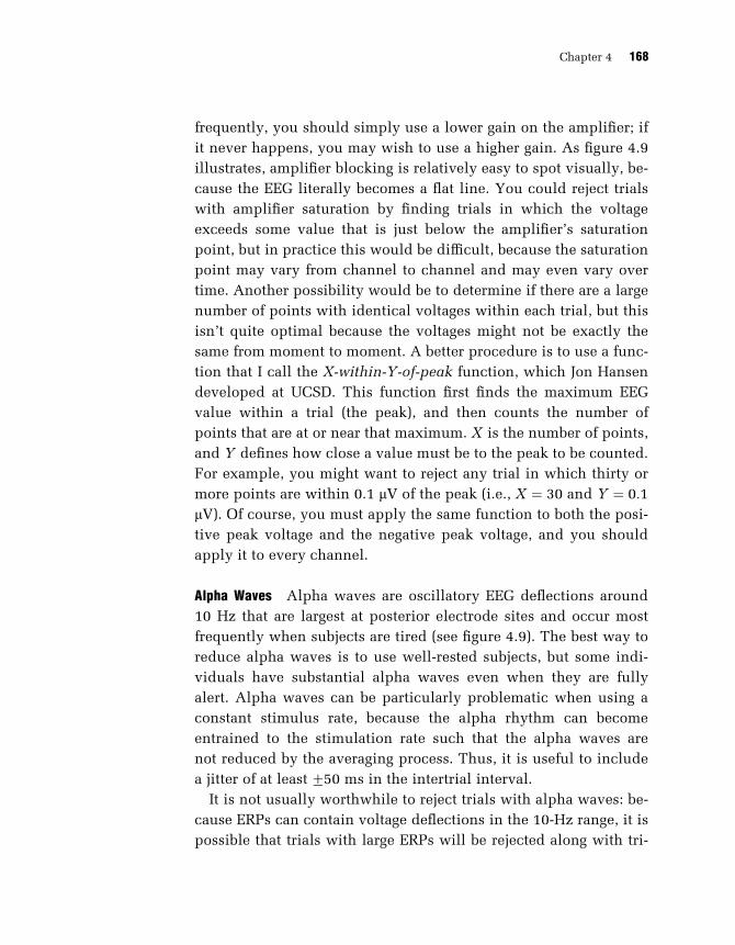
frequently, you should simply use a lower gain on the amplifier; if
it never happens, you may wish to use a higher gain. As figure 4.9
illustrates, amplifier blocking is relatively easy to spot visually, be-
cause the EEG literally becomes a flat line. You could reject trials
with amplifier saturation by finding trials in which the voltage
exceeds some value that is just below the amplifier’s saturation
point, but in practice this would be difficult, because the saturation
point may vary from channel to channel and may even vary over
time. Another possibility would be to determine if there are a large
number of points with identical voltages within each trial, but this
isn’t quite optimal because the voltages might not be exactly the
same from moment to moment. A better procedure is to use a func-
tion that I call the X-within-Y-of-peak function, which Jon Hansen
developed at UCSD. This function first finds the maximum EEG
value within a trial (the peak), and then counts the number of
points that are at or near that maximum. X is the number of points,
and Y defines how close a value must be to the peak to be counted.
For example, you might want to reject any trial in which thirty or
more points are within 0.1 mV of the peak (i.e., X ¼ 30 and Y ¼ 0:1
mV). Of course, you must apply the same function to both the posi-
tive peak voltage and the negative peak voltage, and you should
apply it to every channel.
Alpha Waves Alpha waves are oscillatory EEG deflections around
10 Hz that are largest at posterior electrode sites and occur most
frequently when subjects are tired (see figure 4.9). The best way to
reduce alpha waves is to use well-rested subjects, but some indi-
viduals have substantial alpha waves even when they are fully
alert. Alpha waves can be particularly problematic when using a
constant stimulus rate, because the alpha rhythm can become
entrained to the stimulation rate such that the alpha waves are
not reduced by the averaging process. Thus, it is useful to include
a jitter of at leastG50 ms in the intertrial interval.
It is not usually worthwhile to reject trials with alpha waves: be-
cause ERPs can contain voltage deflections in the 10-Hz range, it is
possible that trials with large ERPs will be rejected along with tri-
Chapter 4 168

als containing alpha artifacts. If it is necessary to reject trials with
alpha, the best procedure is to compute the amplitude at 10 Hz on
each trial and reject trials on which the amplitude exceeds some
threshold value.
Muscle and Heart Activity The voltages created during the contrac-
tion of a muscle are called the electromyogram or EMG (see figure
4.9). These voltages are very high in frequency, and much of the
EMG is usually eliminated by the amplifier’s low-pass filter. You
can also minimize the EMG by asking the subject to relax the
muscles of the neck, jaw, and forehead and by providing a chinrest
or some other device that reduces the load on the neck muscles.4
As discussed above, it is also possible for the subject to recline in
a comfortable chair, but this can cause movements of the posterior
electrodes, resulting in large artifactual voltage shifts. Relaxation of
the muscles below the neck is usually not important, because the
EMG tends not to propagate very far.
It is not usually necessary to reject trials with EMG, assuming
that you have taken appropriate precautions to minimize the EMG.
However, if it is necessary to reject trials with EMG activity, you
can detect EMG in several ways. The best method is to perform a
Fourier transform on each trial and calculate the amount of high-
frequency power (e.g., power above 100 Hz). A simpler method
is to calculate the difference in voltage between every consecutive
pair of points in a given trial and reject the trial if the largest of
these differences exceeds a particular value.
Note that some stimuli will elicit reflexive muscle twitches.
These are particularly problematic because they are time-locked
to the stimulus and are therefore not attenuated by the averaging
process. These also tend to be sudden, high-frequency voltage
changes, but they are usually limited to a very short time period
and are therefore difficult to detect by examining the high-frequency
power across the entire trial. To reject these artifacts, it is best
to look for sudden shifts in voltage during the brief time period
during which they are likely to occur (usually within 100 ms of
stimulus onset).
Averaging, Artifact Rejection, and Artifact Correction 169

The beating of the heart (the EKG) can also be observed in EEG
recordings in some subjects; figure 4.9 shows its distinctive shape.
The EKG is usually picked up by mastoid electrodes, and if a
mastoid is used as a reference, the EKG is seen in inverted form in
all of the electrode sites. The EKG can sometimes be reduced by
slightly shifting the position of the mastoid electrode, but usually
there is nothing that can be done about it. In addition, this artifact
usually occurs approximately once per second during the entire
recording session, so rejecting trials with EKG deflections will usu-
ally lead to the rejection of an unacceptably large proportion of
trials. Fortunately, this artifact is almost never systematic, and it
will simply decrease the overall S/N ratio. In other words, there
isn’t much you can do, and it’s not usually a significant problem,
so don’t worry about it.
The previous paragraph raises an important point. If you see an
artifact or some type of noise equally in all of your EEG channels,
it is probably being picked up by the reference electrode. Most arti-
facts and noise sources will be more prominent at some electrodes
than at others, but any signals picked up by the reference electrode
will appear in inverted form in all electrodes that use that refer-
ence. However, if you are using bipolar recordings for some of
your channels (e.g., for EOG recordings), these recordings will not
have artifacts or noise arising from the main reference electrode.
This can help you identify and eliminate the sources of noise and
artifacts.
Artifact Correction
Artifact rejection is a relatively crude process, because it com-
pletely eliminates a subset of trials from the ERP averages. As Grat-
ton, Coles, and Donchin (1983) discussed, there are three potential
problems associated with rejecting trials with ocular artifacts. First,
in some cases, discarding trials with eye blinks and eye move-
ments might lead to an unrepresentative sample of trials. Second,
there are some groups of subjects (e.g., children and psychiatric
patients) who cannot easily control their blinking and eye move-
Chapter 4 170

ments, making it difficult to obtain a sufficient number of artifact-
free trials. Third, there are some experimental paradigms in which
blinks and eye movements are integral to the tasks, and rejecting
trials with these artifacts would be counterproductive. Under these
conditions, it would be useful to be able to subtract away the vol-
tages due to eye blinks and eye movements rather than rejecting
trials with these artifacts.
Researchers have developed several artifact correction proce-
dures for this purpose (e.g., Berg & Scherg, 1991a, 1994; Gratton,
Coles, & Donchin, 1983; Lins et al., 1993b; Verleger, Gasser, &
Moecks, 1982). When the eyes blink or move, voltages are created
around the eyes that propagate to the scalp electrodes, and the
voltage recorded at a given site will be equal to the value at the
eyes multiplied by a propagation factor, plus any EEG activity
present at that site. The simplest way to correct for eye artifacts is
to calculate the propagation factor between the eyes and each of
the scalp electrodes and subtract a corresponding proportion of
the recorded EOG activity from the ERP waveform at each scalp
site. For example, Lins and colleagues (1993a) found that 47 per-
cent of the voltage present in an EOG recording propagated to the
Fpz electrode, 18 percent to the Fz electrode, and 8 percent to the
Cz electrode. To subtract away the EOG contribution to the aver-
aged ERP waveforms at these electrode sites, it would be possible
to subtract 47 percent of the EOG waveform from the Fpz elec-
trode, 18 percent from the Fz electrode, and 8 percent from the Cz
electrode.
There is a very significant problem with this approach, however.
Specifically, the EOG recording contains brain activity in addi-
tion to true ocular activity and, as a result, the subtraction proce-
dure ends up subtracting away part of the brain’s response as well
as the ocular artifacts. There are additional problems with this
simple-minded subtraction, such as the assumption that the propa-
gation factors will be the same for eye blinks and eye movements (a
problem first addressed by Gratton, Coles, & Donchin, 1983). More
sophisticated versions of this approach address these additional
problems, and can work fairly effectively. For example, one can
Averaging, Artifact Rejection, and Artifact Correction 171

use dipole modeling procedures to isolate the ocular activity (Berg
& Scherg, 1991b), which works fairly well because the approximate
locations of the dipoles are known in advance.
Although these artifact correction techniques can be useful or
even indispensable for certain tasks and certain types of subjects,
they have some significant drawbacks. First, some of these tech-
niques can significantly distort the ERP waveforms and scalp dis-
tributions, making the data difficult to interpret. On the basis of a
detailed comparison of several techniques, Lins et al. (1993b) con-
cluded that source analysis procedures provided the least distor-
tion, and other techniques (such as those of Gratton, Coles, &
Donchin, 1983; Verleger, Gasser, & Moecks, 1982) can yield signifi-
cant distortion. However, even the source analysis procedures may
yield some distortion, especially when non-optimal parameters are
used.
A newer and promising approach is to use independent compo-
nents analysis (ICA). This approach is well justified mathemati-
cally, and recent studies demonstrated that this technique works
very well at removing blinks, eye movements, and even electrical
noise (Jung, Makeig, Humphries et al., 2000; Jung, Makeig, Wester-
field et al., 2000) (see also the similar technique developed by
Joyce, Gorodnitsky, & Kutas, 2004). However, these studies were
conducted by the group who originally developed ICA, so they
may not have been motivated to find conditions under which ICA
performs poorly. In particular, this approach assumes that the
time course of the artifacts is independent of the time course of
the ERP activity, which may not always (or even usually) be a
correct assumption. For example, if detecting a target leads to
both a P3 wave and a blink, the blink and the P3 wave will have
correlated time courses, and this could lead to inaccurate artifact
correction. Until an independent laboratory rigorously tests this
technique, it will be difficult to know whether this sort of situation
leads to significant distortions.
A second problem with artifact correct techniques is that these
techniques may require significant additional effort. For example,
Chapter 4 172

Lins et al. (1993b) recommended that recordings should be ob-
tained from at least seven electrodes near the eyes. In addition,
one must conduct a set of calibration runs for each subject and
carry out extensive signal processing on the data. Thus, it is im-
portant to weigh the time saved by using artifact correction pro-
cedures against the time required to satisfactorily implement these
procedures.
A third problem with these techniques is that they cannot ac-
count for the changes in sensory input caused by blinks and eye
movements. For example, if a subject blinks at the time of a visual
stimulus, then this stimulus may not be seen properly, and this
obviously cannot be accounted for by artifact correction tech-
niques. In addition, as the eyes move, the visual world slides across
the retina, generating a sensory ERP response. Similarly, eye blinks
and eye movements are accompanied by motor ERPs. Artifact cor-
rection procedures do not typically address these factors, which
are especially problematic when task-relevant stimuli trigger the
blinks or eye movements.
Because of these limitations, I would recommend against using
artifact correction procedures unless the nature of the experiment
or subjects makes artifact rejection impossible. When artifact cor-
rection is necessary, I would recommend using one of the newer
and less error-prone techniques, such as ICA or the source localiza-
tion techniques Lins et al. (1993b) discuss. Moreover, I would
strongly recommend against using the simpler techniques that are
often available in commercial ERP analysis packages (such as the
procedure of Gratton et al., 1983). When you use these techniques,
it is difficult to know the extent to which the artifact correction
procedures distort the results.
Suggestions for Further Reading
The following is a list of journal articles and book chapters that
provide useful information about averaging, artifact rejection, and
artifact correction.
Averaging, Artifact Rejection, and Artifact Correction 173
Berg, P., & Scherg, M. (1994). A multiple source approach to the
correction of eye artifacts. Electroencephalography & Clinical
Neurophysiology, 90(3), 229–241.
Gratton, G., Coles, M. G. H., & Donchin, E. (1983). A new method
for off-line removal of ocular artifact. Electroencephalography
and Clinical Neurophysiology, 55, 468–484.
Hillyard, S. A., & Galambos, R. (1970). Eye movement artifact in
the CNV. Electroencephalography and Clinical Neurophysiol-
ogy, 28, 173–182.
Jung, T. P., Makeig, S., Humphries, C., Lee, T. W., McKeown, M. J.,
Iragui, V., & Sejnowski, T. J. (2000). Removing electroencepha-
lographic artifacts by blind source separation. Psychophysiol-
ogy, 37, 163–178.
Jung, T. P., Makeig, S., Westerfield, M., Townsend, J., Courchesne,
E., & Sejnowski, T. J. (2000). Removal of eye activity artifacts
from visual event-related potentials in normal and clinical
subjects. Clinical Neurophysiology, 111, 1745–1758.
Lins, O. G., Picton, T. W., Berg, P., & Scherg, M. (1993). Ocular arti-
facts in EEG and event-related potentials I: Scalp topography.
Brain Topography, 6, 51–63.
Lins, O. G., Picton, T. W., Berg, P., & Scherg, M. (1993). Ocular arti-
facts in recording EEGs and event-related potentials. II: Source
dipoles and source components. Brain Topography, 6, 65–78.
Picton, T. W., Linden, R. D., Hamel, G., & Maru, J. T. (1983).
Aspects of averaging. Seminars in Hearing, 4, 327–341.
Verleger, R., Gasser, T., & Moecks, J. (1982). Correction of EOG
artifacts in event-related potentials of the EEG: Aspects of re-
liability and validity. Psychophysiology, 19(4), 472–480.
Woldorff, M. (1988). Adjacent response overlap during the ERP
averaging process and a technique (Adjar) for its estimation
and removal. Psychophysiology, 25, 490.
Chapter 4 174

5 Filtering
This chapter discusses the application of filters to the EEG during
data acquisition and to ERP waveforms before and after the averag-
ing process. It is absolutely necessary to use filters during data ac-
quisition, and it is very useful to apply filters offline as well, but
filtering can severely distort ERPs in ways that ERP researchers
frequently do not appreciate. For example, filters may change the
onset and duration of an ERP component, may make monophasic
waveforms appear multiphasic, may induce artificial oscillations,
and may interfere with the localization of generator sources. This
chapter will explain how these distortions arise and how they can
be prevented. To avoid complex mathematics, I will simplify the
treatment of filtering somewhat in this chapter, but there are sev-
eral books on filtering that the mathematically inclined reader may
wish to read (e.g., Glaser & Ruchkin, 1976). Note also that the term
filter can refer to any of a large number of data manipulations, but
this chapter will be limited to discussing the class of filters that
ERP researchers typically use to attenuate specific ranges of fre-
quencies, which are known as finite impulse response filters.
ERP waveforms are generally conceptualized and plotted as
time-domain waveforms, with time on the X axis and amplitude
on the Y axis. In contrast, filters are typically described in the
frequency-domain, with frequency on the X axis and amplitude or
power on the Y axis.1 Because ERP researchers are typically more
interested in temporal information rather than frequency informa-
tion and because temporal information may be seriously distorted
by filtering, it is important to understand filtering as a time-domain
operation as well as a frequency-domain operation.2 This chap-
ter therefore describes how filters operate in both the time and

frequency domains, as well as the relationship between these
domains. I will focus primarily on the digital filters that are used
for offline filtering, but the principles discussed here also apply to
the analog filters that are found in amplifiers. My goal in this chap-
ter is to provide an intuitive understanding of how filters work,
and I have therefore minimized the use of equations as much as
possible and limited the equations to simple algebra. If you under-
stand how summations work (i.e., the S symbol), then you know
enough math to understand this chapter.
Even though an advanced math background is not necessary to
understand this chapter, some of the concepts are pretty compli-
cated. As a result, you may not want to spend the time required to
understand exactly how filters work and exactly why they distort
ERP waveforms in particular ways, especially on your first pass
through the book. If so, you can just read the next two sections
(‘‘Why Are Filters Necessary’’ and ‘‘What Everyone Should Know
About Filtering’’). These sections will provide enough information
to keep you from getting into too much trouble with filters, and you
can read the rest of the chapter later.
Why Are Filters Necessary?
The most important message of this chapter is that filters can sub-
stantially distort ERP data. Given that this is true, it is useful to ask
why filters are necessary in the first place. There are two answers
to this question, the first of which is related to the Nyquist Theo-
rem, discussed previously in chapter 3. This theorem states that it
is possible to convert a continuous analog signal (such as the EEG)
into a set of discrete samples without losing any information, as
long as the rate of digitization is at least twice as high as the
highest frequency in the signal being digitized. This is fundamen-
tally important for the data acquisition process, because it means
that we can legitimately store the EEG signal as a set of discrete
samples on a computer. However, this theorem also states that if
the original signal contains frequencies that are more than twice
as high as the digitization rate, these very high frequencies will
Chapter 5 176

appear as artifactual low frequencies in the digitized data (this is
called aliasing). Consequently, EEG amplifiers have filters that one
can use to suppress high frequencies; these filters are generally set
to attenuate frequencies that are higher than a half of the sampling
rate. For example, in a typical cognitive ERP experiment, the digi-
tization rate might be 250 Hz, and it would therefore be necessary
to make sure that everything above 125 Hz is filtered. It would be
tempting to choose a filter cutoff frequency of 125 Hz, but a cutoff
frequency of 125 Hz just means that the power (or amplitude) has
been reduced by 50 percent at 125 Hz, and there will be consider-
able remaining activity above 125 Hz. It is therefore necessary to
select a substantially lower value such as 80 Hz (in practice, the
digitization rate should be at least three times as high as the cutoff
value of the filter).
The second main goal of filtering is the reduction of noise, and
this is considerably more complicated. The basic idea is that the
EEG consists of a signal plus some noise, and some of the noise is
sufficiently different in frequency content from the signal that it
can be suppressed simply by attenuating certain frequencies. For
example, most of the relevant portion of the ERP waveform in a
typical cognitive neuroscience experiment consists of frequencies
between 0.01 Hz and 30 Hz, and contraction of the muscles leads
to an EMG artifact that primarily consists of frequencies above 100
Hz; consequently, the EMG activity can be eliminated by suppress-
ing frequencies above 100 Hz and this will cause very little change
to the ERP waveform. However, as the frequency content of the sig-
nal and the noise become more and more similar, it becomes more
and more difficult to suppress the noise without significantly
distorting the signal. For example, alpha waves can provide a sig-
nificant source of noise, but because they are around 10 Hz, it is
difficult to filter them without significantly distorting the ERP
waveform. Moreover, even when the frequency content of the
noise is very different from that of the signal, the inappropriate
application of a filter can still create significant distortions.
In addition to suppressing high frequencies, filters are also used
in most experiments to attenuate very low frequencies. The most
Filtering 177

common use of such filters is to remove very slow voltage changes
of non-neural origin during the data acquisition process. Specifi-
cally, factors such as sweating (which creates skin potentials) and
drifts in electrode impedance can lead to slow, sustained changes
in the baseline voltage of the EEG signal, and it is usually a good
idea to remove these slow voltage shifts by filtering frequencies
lower than approximately 0.01 Hz. This is especially important
when obtaining recordings from patients or from children, because
head and body movements are one common cause of these sus-
tained shifts in voltage. If these shifts are not eliminated, they may
cause the amplifier to saturate and data to be lost. Even if they do
not cause amplifier saturation, they are very large voltages and
may cause large distortions in the average ERP waveforms. Thus,
it is almost always a good idea to filter the very low frequencies
(< 0.01 Hz).
What Everyone Should Know about Filtering
Any waveform can be decomposed into a set of sine waves of
various frequencies and phases, and the waveform can be recon-
structed by simply summing these sine waves together. Filters are
usually described in terms of their ability to suppress or pass
various different frequencies. The most common types of filters
are: (1) low-pass filters, which attenuate high frequencies and pass
low frequencies; (2) high-pass filters, which attenuate low frequen-
cies and pass high frequencies; (3) bandpass filters, which attenu-
ate both high and low frequencies, passing only an intermediate
range of frequencies; and (4) notch filters, which attenuate some
narrow band of frequencies and pass everything else.
Filters and Amplitude Attenuation
The properties of a filter are usually expressed by its transfer func-
tion, the function that determines how the input of the filter is
‘‘transferred’’ to the output of filter. The transfer function can be
Chapter 5 178

broken down into two components, a frequency response function
that specifies how the filter changes the amplitude of each fre-
quency, and a phase response function that specifies how the filter
changes the phase of each frequency. Figure 5.1A shows an exam-
ple of the frequency response function of a low-pass filter with a
half-amplitude cutoff at 30 Hz, and it also shows how this filter
suppresses 60-Hz noise in an actual ERP waveform. In ERP re-
search, a filter is often described only in terms of its half-amplitude
cutoff, which is the frequency at which the amplitude is cut by 50
percent (sometimes the cutoff frequency is specified in terms of
power rather than amplitude; amplitude reaches 71 percent when
power reaches 50 percent). As figure 5.1A illustrates, however,
there is quite a bit of attenuation at frequencies below the half-
amplitude cutoff, and the attenuation is far from complete for
frequencies quite a bit higher than the half-amplitude cutoff. None-
theless, this filter effectively suppresses the 60-Hz noise in the
waveform while retaining the waveform’s basic shape.
Figure 5.1B shows the frequency response function of a high-
pass filter with a half-amplitude cutoff at approximately 2.5 Hz
and the effect of this filter on an ERP waveform. As you can see,
the large, broad upward deflection (similar to a P3 wave) is greatly
reduced in amplitude by this filter, whereas the initial, higher
frequency deflections (similar to P1 and N1 waves) are not reduced
as much. However, the amplitudes of the earlier components are
influenced somewhat, and small artifactual peaks have been cre-
ated at the beginning and end of the waveform. This leads to the
most important point of this section: filters can significantly distort
ERP waveforms, changing the amplitude and timing of the ERP
components and adding artifactual peaks.
High-pass filters are often described in terms of their time
constants rather than their half-amplitude cutoffs. As figure 5.1C
shows, if the input to a high-pass filter is a constant voltage, the
output of the filter will start at this voltage and then gradually
return toward zero, and the filter’s time constant is a measure of
the rate at which this occurs. The decline in output voltage over
Filtering 179

Half-amplitudecutoff = 30 Hz
0.50
1.00
0.75
0.25
0.000 20 40 60 80 100
A
Frequency (Hz)
Gain
Unfiltered ERPwaveform
Filtered ERPwaveform
0
Frequency (Hz)5 1510
0.50
1.00
0.75
0.25
0.00
Gain
Half-amplitudecutoff = 2.5 Hz
Unfiltered ERPwaveform
Filtered ERPwaveform
B
0.50
1.00
0.75
0.25
0.00
FilterInput(µV)
Time (seconds)
0.50
1.00
0.75
0.25
0.00
FilterOutput(µV) 37%
CTime constant =
3.6 seconds
0Time Poststimulus (ms)
200 400 600
Original waveform, band pass of .01 - 80 Hz
Low-pass filtered,half-amplitude cutoff = ~40 Hz
Low-pass filtered,half-amplitude cutoff = ~10 Hz
Low-pass filtered,half-amplitude cutoff = ~20 Hz
D
0 2 640
Time (seconds)2 4 6
Chapter 5 180

time is exponential, so the value never quite reaches zero. Conse-
quently, the time constant is expressed as the time required for the
filter’s output to reach 1=e (37 percent) of the starting value. As the
half-amplitude cutoff becomes higher, the time constant becomes
shorter. If you know the half-power cutoff frequency of a high-pass
filter ( fc, the frequency at which the filter’s output is reduced by 3
dB), the time constant can be computed as 1=ð2pfcÞ.
Filters and Latency Shift
So far, we have focused on the effects of filters on the amplitude at
each frequency, but it also important to keep in mind that filters
usually influence the phase (time shift) at each frequency as well.
In particular, all analog filters (such as those in EEG amplifiers)
shift the latency of the signal, and most analog filters shift the
latency by different amounts for different frequencies. These shifts
become more pronounced as the cutoff frequency of a low-pass
filter is made lower and the cutoff frequency of a high-pass filter is
made higher. In contrast, most digital filters (filters that are applied
offline) do not cause a phase shift. Thus, it is usually best to do as
little filtering as possible prior to digitizing the data and to do most
of the filtering offline.
How Filters Are Used
Some filtering is essential in amplifying and digitizing the EEG
signal. First, it is necessary to filter out high frequencies with
a low-pass filter before digitizing the data to ensure that the
H Figure 5.1 Basics of filtering. (A) Frequency response function of a low-pass filter with a half-amplitude cutoff at 30 Hz, and application of this filter to an ERP waveform. (B) Fre-quency response function of a high-pass filter with a half-amplitude cutoff at 2.5 Hz,and application of this filter to an ERP waveform. (C) Example of the time constantof a high-pass filter. A constant input to the filter is shown on the left, and thedecaying output of the filter is shown on the right. (D) Noisy ERP waveform low-pass filtered with various half-amplitude cutoffs.
Filtering 181

sampling rate is at least twice as high as the highest frequency in
the signal. Second, it is almost always necessary to filter out very
low frequencies (e.g., <0.01 Hz) so that slow, non-neural electrical
potentials (e.g., skin potentials) do not bring the signal outside of
the operating range of the amplifier and analog-to-digital converter.
ERP researchers also frequently use a line frequency filter, a notch
filter that filters out noise generated by AC electrical devices (usu-
ally 50 Hz or 60 Hz). As I will discuss later in this chapter, how-
ever, notch filters significantly distort the data and should be
avoided if possible. Chapter 3 described some strategies for elimi-
nating electrical noise at the source, but if it is impossible to
reduce line-frequency noise sufficiently, a low-pass filter with a
half-amplitude cutoff at 30 Hz can effectively filter out the noise
without distorting the data as much as a notch filter.
ERP researchers sometimes use low-pass and high-pass filters to
‘‘clean up’’ noisy data. For example, figure 5.1D shows an ERP
waveform that was mildly filtered (.01–80 Hz) prior to amplifica-
tion and the same waveform after it was low-pass filtered offline
with progressively lower cutoff frequencies. As the cutoff fre-
quency decreases, the waveform becomes smoother and generally
nicer looking. From this example, you might think that filtering is
a good thing. However, the most important thing that I would like
to communicate in this chapter is that filtering always distorts the
ERP waveform, and the more heavily the data are filtered, the
worse the distortion will be.
How Filters Can Distort Your Data
The distortions caused by filtering can be summarized by a key
principle that you should commit to memory now and recall every
time the topic of filtering comes up: precision in the time domain is
inversely related to precision in the frequency domain. In other
words, the more tightly you constrain the frequencies in an ERP
waveform (i.e., by filtering out a broad range of frequencies), the
more the ERP waveform will become spread out in time. Figure
Chapter 5 182

5.2A illustrates one type of spreading, showing how low-pass fil-
tering an ERP waveform causes the filtered waveform to start ear-
lier and end later than the unfiltered waveform. Low-pass filters
almost always have this effect of ‘‘smearing out’’ the waveform
and distorting the onset and offset times of the ERP components
and experimental effects. Thus, if you see that an experimental
effect starts at 120 ms in low-pass filtered waveforms, the effect
may have actually started at 150 ms.
B
A
Unfiltered
Filtered
Unfiltered
Filtered
0
Frequency (Hz)10 3020
0.50
1.00
0.75
0.25
0.00
Gain
C
Figure 5.2 Examples of distortions caused by filtering. (A) Effects of low-pass filtering on onsetand offset times of an ERP waveform. (B) Artifactual oscillations caused by a high-pass filter. (C) Frequency response function of the filter used in (B).
Filtering 183

As figure 5.2B illustrates, high-pass filters also cause the ERP
waveform to become spread out in time, but the distortion in
this case consists of a series of up and down sinusoidal deflec-
tions. Thus, not only did this particular filter cause artifactual
activity to begin well before the actual onset of activity, it created
the appearance of oscillations in the waveform. This sort of effect
could also cause an experimental effect in a component of one
polarity to appear as an effect in an earlier component of opposite
polarity (e.g., an increase in N1 amplitude in the original wave-
form might appear as an increase in P1 amplitude in the filtered
waveform). As you can imagine, using this sort of filter might
cause someone to completely misinterpret the results of an ERP
experiment.
High-pass filters do not always create artifactual oscillations.
For example, the high-pass filter shown in figure 5.1B produces a
single opposite-polarity artifactual deflection at each end of the
ERP waveform rather than a multi-peaked oscillation. The long-
lasting and oscillating pattern of distortion the filter shown in
figure 5.2B creates is a consequence of the filter’s frequency re-
sponse function, which is shown in figure 5.1C. Whereas the filter
in figure 5.1B has a relatively gradual transition between suppress-
ing the lowest frequencies and passing higher frequencies, the filter
in figure 5.2B completely blocks a fairly broad set of low frequen-
cies and then suddenly starts passing higher frequencies. That is,
the filter in figure 5.2B has more precision in terms of its frequency
properties than the filter in figure 5.1B, and this brings us back to
the principle that precision in the time and frequency domains are
inversely related. That is, more sudden changes in a filter’s fre-
quency response function lead to broader temporal distortions in
the ERP waveform. Thus, a filter with a really sharp cutoff in its
frequency response function might seem to be ideal, but a sharp
cutoff usually means that the filter will cause more severe distor-
tion of the ERP waveform than a filter with a gentler cutoff. Makers
of commercial ERP systems often tout the sharp cutoffs of their
filters, but such filters are usually a bad idea.
Chapter 5 184

If you want to see how a filter might be distorting your ERP
waveforms, the easiest thing to do is to pass some sort of known,
artificial waveform through the filter and compare the original and
filtered waveforms. For example, many amplifiers contain calibra-
tors that produce a single pulse of a square wave, and you can
record this and filter it with various types of filters.
Recommendations
Now that I’ve discussed why filters are used and how they can dis-
tort your data, I will make some specific recommendations. These
recommendations might not be appropriate for every experiment,
but they should be appropriate for the vast majority of ERP experi-
ments in cognitive neuroscience.
First, keep Hansen’s Axiom in mind: There is no substitute for
clean data (see chapter 3). Some minor filtering is necessary when
first collecting the data, and a modest amount of additional filter-
ing can be helpful under some conditions. However, filters cannot
help you if your data are noisy because of variability across sub-
jects, variability across trials, a small number of trials in your aver-
ages, and so on. Filters may make the data look better under these
conditions, but this will be an illusion that may lead you to draw
incorrect conclusions.
Second, during the amplification and digitization process, you
should do as little filtering as possible. It’s always possible to filter
the data more offline, but you can never really ‘‘unfilter’’ data that
have already been filtered. The low-pass filter should be set at be-
tween one third and one fourth of the sampling rate (and I would
recommend a sampling rate of between 200 and 500 Hz for most
experiments). For experiments with highly cooperative subjects
(e.g., college students), I would recommend using a high-pass filter
of 0.01 Hz. Some amplifiers allow you to do no high-pass filtering
at all (these are called DC recordings), but unless you are looking
at very slow voltage shifts, this will lead to an unacceptable level
of noise due to skin potentials and other slow artifacts.
Filtering 185

If you are recording from less cooperative subjects (e.g., patients
or children), you may need to use a higher high-pass cutoff, such
as 0.05 Hz or even 0.1 Hz. The main problem with such subjects
is that they may move around a lot, which causes changes in the
baseline electrical potential that will slowly resolve over time.
This creates a lot of noise in the data that averaging may not suffi-
ciently attenuate, and it can also lead the amplifiers to saturate. But
if you use a higher high-pass cutoff, be aware that this is distort-
ing your data somewhat and reducing the amplitude of the lower-
frequency components, such as the P3 and N400 waves. Indeed,
Duncan-Johnson and Donchin (1979) showed many years ago that
relatively high cutoff frequencies lead to a substantial reduction in
apparent P3 amplitude.
During amplification, you should avoid using a notch filter (also
called a line-frequency filter) to reduce line-frequency noise. These
filters can cause substantial distortion of the ERP waveform. As
chapter 3 described, there are various precautions you can take to
eliminate line-frequency noise before it enters the EEG, and this is
the best approach. However, you may sometimes be faced with
such a huge level of line-frequency noise that the incoming EEG is
completely obscured, and on such occasions you may need to use a
notch filter to eliminate this noise.
My third recommendation is to keep offline filtering to a mini-
mum. If the averaged ERP waveforms are a little fuzzy looking,
making it difficult to see the experimental effects, it can be helpful
to apply a low-pass filter with a half-amplitude cutoff somewhere
between 20 and 40 Hz. This can dramatically improve the appear-
ance of the ERP waveforms when you plot them, and the temporal
distortion should be minimal (especially if you use a filter with a
relatively gentle cutoff). This sort of filtering will also be helpful if
you are using peak amplitude or peak latency measures, but it is
unnecessary if you are using mean amplitude or fractional area
latency measures (see chapter 6 for more details). In fact, because
filters spread out an ERP waveform, measuring the mean ampli-
tude in a particular latency range from filtered waveforms (e.g.,
Chapter 5 186

200–250 ms poststimulus) is equivalent to measuring the mean
amplitude from a broader range in the original unfiltered wave-
forms (e.g., 175–275 ms). My laboratory typically uses a low-pass
filter with a half-amplitude cutoff at 30 Hz for plotting the data,
but no offline filtering for measuring component amplitudes.
My fourth recommendation is to avoid using high-pass filters
altogether (except during data acquisition, as described above).
High-pass filters are much more likely than low-pass filters to
cause major distortions of your ERP waveforms that might lead
you to draw incorrect conclusions about your data. There are occa-
sions when high-pass filters can be useful, such as when dealing
with overlapping activity from preceding and subsequent stimuli.
However, high-pass filters are sufficiently dangerous that you
should use them only if you really understand exactly what they
are doing. The remainder of this chapter will help provide you
with this understanding.
Filtering as a Frequency-Domain Procedure
The key to understanding filters is to understand the relation-
ship between the time domain and the frequency domain. A time-
domain representation of an ERP is simply a plot of the voltage at
each time point, as figure 5.3A illustrates. A frequency-domain
representation of an ERP is a plot of the amplitude (and phase)
at each frequency, as figure 5.3B illustrates. Time-domain and
frequency-domain representations contain exactly the same infor-
mation, viewed from different perspectives, and it is possible to
transform one type of representation into the other via Fourier
analysis, a technique developed in the 1800s by the mathematician
Joseph Fourier.
The basic principle of Fourier analysis is that any time-domain
waveform can be exactly represented by the sum of a set of sine
waves of different frequencies and phases. In other words, it is pos-
sible to create any waveform (even a momentary spike or a square
wave) by adding together a set of sine waves of varying frequencies
Filtering 187

B
D
E
Unfiltered ERPwaveform
Transformation of Ainto frequency domain
C
Frequency responsefunction of filter
Product offunctions B and C
Transformation of Dinto time domain
A
0.50
1.00
0.75
0.25
0.000 20 40 60 80 100
0.50
1.00
0.75
0.25
0.000 20 40 60 80 100
0.50
1.00
0.75
0.25
0.000 20 40 60 80 100
1000 200 300 400 500
1000 200 300 400 500
Chapter 5 188

and phases. The Fourier transform is a mathematical procedure
that takes a time-domain signal (such as an ERP waveform) as an
input and computes the amplitudes and phases of the sine waves
that would need to be added together to recreate the input wave-
form. As figure 5.3B illustrates, the output of the Fourier transform
is usually shown as a plot of amplitude and phase3 as a function of
frequency. It is also possible to use the inverse Fourier transform to
convert a frequency-domain representation back into the original
time-domain representation, thus obtaining the original voltagetime ERP waveform.
In the context of Fourier analysis, one can conceptualize filtering
as a series of three steps:
1. The time-domain ERP waveform is converted into a frequency-
domain representation.
2. The to-be-filtered frequency range is set to zero in the frequency-
domain representation.
3. The modified frequency-domain representation is converted back
into the time domain.
This completely eliminates one set of frequencies from the ERP
waveform without influencing the other frequencies. As I will dis-
cuss in detail below, a sudden drop-off in the frequency domain
leads to some undesirable consequences, so it is necessary to add
a slight complication to this three-step procedure. Specifically,
H Figure 5.3 Example of the frequency-domain conceptualization of filtering. (A) Unfiltered ERPwaveform, contaminated by substantial noise at 60 Hz. (B) Transformation of (A)into the frequency domain, with a clear peak at 60 Hz. (C) Frequency response func-tion of a filter that can be used to remove the 60-Hz noise from (B) while retainingmost of the signal, which is primarily confined to frequencies below 20 Hz. (D)Product of (B) and (C); for each frequency point, the magnitude in (B) is multipliedby the magnitude in (C). Note that (D) is nearly identical to (B) in the low frequencyrange, but falls to zero at high frequencies. (E) Transformation of (D) back into thetime domain, where it closely resembles the original ERP waveform in (A), exceptfor the absence of the 60-Hz noise. Note that the phase portion of the frequency-domain plots has been omitted here for the sake of simplicity, although the phaseinformation is crucial for transforming between the time and frequency domains.
Filtering 189

rather than setting some range of frequencies to zero and leaving
the other frequencies untouched, it is useful to shift gradually
from no attenuation to complete attenuation. The function that
defines this gradual shift in attenuation as a function of frequency
is called the frequency response function of a filter. More specifi-
cally, the frequency response function contains a scaling factor for
each frequency that represents the extent to which that frequency
will be passed by the filter, with a value of 1 for frequencies that
will be unaffected by the filter, a value of zero for frequencies that
will be completely suppressed, and an intermediate value for fre-
quencies that will be partially attenuated. This function is used in
step two of the filtering process: rather than setting some frequen-
cies to zero, the frequency response function is multiplied by the
frequency-domain representation of the ERP waveform to attenuate
each frequency by a specific amount (i.e., each frequency in the
ERP is multiplied by the corresponding scaling factor in the fre-
quency response function).
Figure 5.3 illustrates this approach to filtering. Panel A shows a
time-domain representation of an unfiltered ERP waveform, which
contains an obvious 60-Hz noise oscillation. Panel B shows the
Fourier transform of this waveform. Note that most of the power is
at low frequencies (< 20 Hz), with a spike at 60 Hz corresponding
to the noise oscillation in the time-domain waveform. Panel C
shows the frequency response function of a filter that passes the
very lowest frequencies and then gradually falls off at higher fre-
quencies. Panel D shows the result of multiplying the frequency-
domain representation of the ERP waveform (i.e., panel B) by the
frequency response function of the filter (i.e., panel C). Note that
the result is very similar to the waveform in panel B, but the spike
at 60 Hz is missing. Panel E shows the result of applying the
inverse Fourier transform to the waveform in panel D, which
converts the frequency-domain representation back into the time
domain. The result is an ERP waveform that is very similar to
the original waveform in panel A, but without the 60-Hz noise
oscillation.
Chapter 5 190

Note that it is possible to use any set of scaling factors for the
frequency response function shown in figure 5.3C. For example,
you could set all of the odd-numbered frequencies to 1 and all of
the even-numbered frequencies to zero, or you could use the
profile of the Rocky Mountains near Banff to determine the scaling
factors. In practice, however, frequency response functions are
usually smoothly descending (low-pass filters), smoothly ascend-
ing (high-pass filters), flat at 1.0 except for a notch (notch filters),
or flat at 0.0 for the lowest and highest frequencies with a single
peak at intermediate frequencies (band-pass filters).
The above discussion has concentrated on the amplitude of each
frequency and has neglected phase. A frequency-domain represen-
tation actually has two parts, one representing the amplitude at
each frequency and the other representing the phase at each fre-
quency. Filters may shift the phases of the frequencies as well as
modulating their amplitudes, and to fully characterize a filter in
the frequency domain, it is necessary to specify its transfer func-
tion, which specifies both the frequency gain and the phase shift
at each frequency. It is usually desirable for the phase portion of
the transfer function to be zero for all frequencies, thereby leaving
the phases from the ERP waveform unchanged. This is usually
possible when digital filters are applied offline, but is impossible
when analog filters are applied online (e.g., when low and high
frequencies are removed from the EEG during data acquisition).
However, certain analog filters have transfer functions in which
the phase portion increases linearly as a function of frequency
(e.g., Bessel filters), which means that all frequencies are shifted
by the same amount of time; the output of such filters can be
shifted back by this amount during the averaging process, thus
eliminating the phase shift produced by the filter.
A Problem with Frequency-Domain Representations
Although it is mathematically convenient to conceptualize filtering
as a frequency-domain procedure, this approach has an important
Filtering 191

shortcoming when applied to transient ERP waveforms. The diffi-
culty stems from the fact that time-domain waveforms are repre-
sented in Fourier analysis as the sum of a set of infinite-duration
sine waves, whereas transient ERP waveforms are finite in dura-
tion. Although the Fourier representation is accurate in the sense
that ERPs can be transformed between the time and frequency
domains with no loss of information, it is inaccurate in the sense
that ERPs actually consist of finite-duration voltage deflections
rather than sets of infinite-duration sine waves. The biologically
unrealistic nature of the frequency-domain representation leads to
a number of problems that I will discuss in this chapter.
At this point, let’s consider a particularly extreme case in which
activity at precisely 5 Hz is filtered from an ERP waveform. Com-
pletely suppressing the 5-Hz component of an ERP waveform
would be equivalent to computing the amplitude and phase in the
5-Hz frequency band and then subtracting a sine wave with this
amplitude and phase from the time-domain ERP waveform. After
subtraction of this infinite-duration sine wave, the resulting wave-
form would contain a 5-Hz oscillation during intervals where the
unfiltered ERP waveform was flat, such as the prestimulus interval.
This is counterintuitive, because filtering out the activity at 5 Hz
actually creates a 5-Hz oscillation in the prestimulus interval.
Moreover, because the response to a stimulus obviously cannot
precede the stimulus in time, this prestimulus oscillation reflects
an impossible state of affairs. Thus, because Fourier analysis repre-
sents transient ERP waveforms as the sum of infinite-duration sine
waves, which is a biologically incorrect representation, the use of
analytical techniques based on frequency-domain representations
may lead to serious distortions.
As discussed earlier in this chapter, an important rule for under-
standing the distortion that filters may produce is that there is an
inverse relationship between the spread of a signal in the time
domain and the spread of the same signal in the frequency domain;
a signal that is tightly localized in time will be broadly localized in
Chapter 5 192
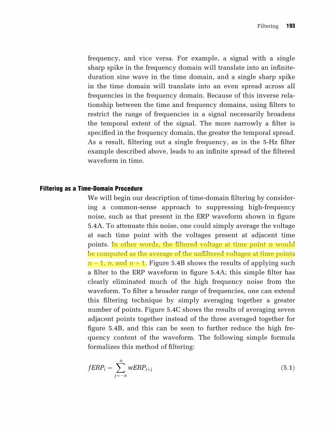
frequency, and vice versa. For example, a signal with a single
sharp spike in the frequency domain will translate into an infinite-
duration sine wave in the time domain, and a single sharp spike
in the time domain will translate into an even spread across all
frequencies in the frequency domain. Because of this inverse rela-
tionship between the time and frequency domains, using filters to
restrict the range of frequencies in a signal necessarily broadens
the temporal extent of the signal. The more narrowly a filter is
specified in the frequency domain, the greater the temporal spread.
As a result, filtering out a single frequency, as in the 5-Hz filter
example described above, leads to an infinite spread of the filtered
waveform in time.
Filtering as a Time-Domain Procedure
We will begin our description of time-domain filtering by consider-
ing a common-sense approach to suppressing high-frequency
noise, such as that present in the ERP waveform shown in figure
5.4A. To attenuate this noise, one could simply average the voltage
at each time point with the voltages present at adjacent time
points. In other words, the filtered voltage at time point n would
be computed as the average of the unfiltered voltages at time points
n 1, n, and nþ 1. Figure 5.4B shows the results of applying such
a filter to the ERP waveform in figure 5.4A; this simple filter has
clearly eliminated much of the high frequency noise from the
waveform. To filter a broader range of frequencies, one can extend
this filtering technique by simply averaging together a greater
number of points. Figure 5.4C shows the results of averaging seven
adjacent points together instead of the three averaged together for
figure 5.4B, and this can be seen to further reduce the high fre-
quency content of the waveform. The following simple formula
formalizes this method of filtering:
fERPi ¼X
n
j¼n
wERPiþj ð5:1Þ
Filtering 193

B
1000 200 300 400
A
1000 200 300 400
C
1000 200 300 400
D
1000 200 300 400
Figure 5.4 Example of filtering an ERP waveform by averaging together the voltages surround-ing each time point. (A) Unfiltered ERP waveform, contaminated by substantial high-frequency noise. (B) Result of filtering the waveform in (A) by averaging the voltageat each time point with the voltages at the immediately adjacent time points. (C) Re-sult of filtering the waveform in (A) by averaging the voltage at each time point withthe voltages at the three time points on either side. (D) High-pass-filtered waveform,constructed by subtracting the filtered waveform in (C) from the unfiltered waveform(A).
Chapter 5 194

where: fERPi is the filtered ERP waveform at time i; ERPi is the
unfiltered ERP waveform at time i; n is the number of points to be
averaged together on each side of the current time point; and
w ¼ 1=ð2nþ 1Þ (which is the weighting value).
This equation states that the filtered voltage at a given time point
is computed by multiplying each of the n voltages on either side of
the current time point and the value at the current time point by
the weighting value w and then adding together these weighted
values. This is equivalent to averaging these 2nþ 1 points (n points
before the current point þ n points after the current point þ the
current point ¼ 2nþ 1).
It is worth spending some time to make sure that you understand
equation 5.1. Once you understand it, you will have understood
the essence of digital filtering.
One can extend this filtering technique in a straightforward
manner to attenuate low frequencies instead high frequencies. The
unfiltered waveform is equal to the sum of its high frequency
components and its low frequency components; as a result, one
can filter out the low frequencies by simply subtracting the low-
pass-filtered waveform from the unfiltered waveform. Figure 5.4D
shows the result of this form of high-pass filtering, which is equal
to the waveform in figure 5.4A minus the waveform in figure 5.4C.
When filtering is accomplished by simply averaging together the
2nþ 1 points surrounding each time point, all of the time points
being averaged together contribute equally to the filtered value at
the current time point, and this reduces the temporal precision of
the filtered waveform. To mitigate this problem, one can use a
weighted average that emphasizes nearby time points more than
distant time points. For example, a three-point filter might use
weights of 0.25 for the two adjacent points and a weight of 0.50 for
the current point (note that our original filter used equal weights of
0.33 for all three time points). In the general case, we can define an
array W that contains 2nþ 1 weights, and recast our filtering for-
mula as:
Filtering 195

fERPi ¼X
n
j¼n
WjERPiþj ð5:2Þ
Our three-point weighting function would then be defined as:
W1 ¼ :25; W0 ¼ :50; Wþ1 ¼ :25
For an equal weighting over 2nþ 1 time points, as in our original
formulation, the weighting function would be:
Wj ¼1
2nþ 1
You can use virtually any conceivable weighting function for
filtering, and the shape of this function will determine the proper-
ties of the filter. As I will describe below, there is a straightforward
relationship between the shape of the weighting function and the
frequency response function of the filter.
In addition to computing the filtered value at a given time point,
it is sometimes useful to consider how the unfiltered value at a
given time point influences the filtered values at surrounding time
points. If we reverse the weighting function in time, the resulting
function represents the effect of the current point on the output of
the filter. This reversed weighting function is equivalent to the
waveform that the filter would produce in response to a momen-
tary voltage spike or impulse; it is therefore known as the impulse
response function of the filter.
Figure 5.5 illustrates the relationship between the weighting
function and the impulse response function. Panel A shows a
weighting function, and panel B shows the corresponding impulse
response function. In addition, panel C shows the output of the
filter if the input is a momentary impulse. Note that the output of
the filter becomes non-zero before the impulse, which is possible
only with an off-line, digital filter. Analog filters that operate in
real time have impulse response functions that are zero before the
time of the impulse.
Chapter 5 196
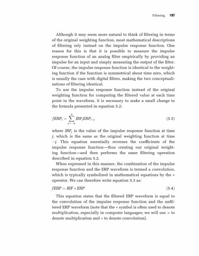
Although it may seem more natural to think of filtering in terms
of the original weighting function, most mathematical descriptions
of filtering rely instead on the impulse response function. One
reason for this is that it is possible to measure the impulse
response function of an analog filter empirically by providing an
impulse for an input and simply measuring the output of the filter.
Of course, the impulse response function is identical to the weight-
ing function if the function is symmetrical about time zero, which
is usually the case with digital filters, making the two conceptuali-
zations of filtering identical.
To use the impulse response function instead of the original
weighting function for computing the filtered value at each time
point in the waveform, it is necessary to make a small change to
the formula presented in equation 5.2:
fERPi ¼X
n
j¼n
IRFjERPij ð5:3Þ
where IRFj is the value of the impulse response function at time
j, which is the same as the original weighting function at time
j. This equation essentially reverses the coefficients of the
impulse response function—thus creating our original weight-
ing function—and then performs the same filtering operation
described in equation 5.2.
When expressed in this manner, the combination of the impulse
response function and the ERP waveform is termed a convolution,
which is typically symbolized in mathematical equations by the operator. We can therefore write equation 5.3 as:
fERP ¼ IRF ERP ð5:4Þ
This equation states that the filtered ERP waveform is equal to
the convolution of the impulse response function and the unfil-
tered ERP waveform (note that the symbol is often used to denote
multiplication, especially in computer languages; we will use to
denote multiplication and to denote convolution).
Filtering 197

Time Point relative to currenttime point
Wei
ght
Weighting function
0 +1-1-2-3-4 +2
Wei
ght
Impulse response function
+2 +3+10-1-2 +4
B
D
A
E
Unfiltered ERPWaveform
Impulse(filter input)
Scaled impulseresponse function
(filter output)
C
Filter Output = Sum of ScaledImpulse Response Functions
Time Point relative to currenttime point
Scaled Copies of ImpulseResponse Function at
Individual Sample Points
Chapter 5 198

The filtering equations listed above are written in a manner that
makes it easy to see how the filtered value at a given time point is
computed from the unfiltered values at surrounding time points. It
is also possible to take a complementary approach and compute
the contribution of a given unfiltered time point to the filtered
waveform. Although less useful computationally, this approach
more readily allows one to visualize the relationship between a
filter’s impulse response function and the filtered ERP waveform.
In this approach, each point in the unfiltered waveform is replaced
by a scaled copy of the impulse response function (scaled by the
amplitude of the unfiltered waveform at the current time point).
These scaled copies of the impulse response function are then
simply added together to compute the filtered ERP waveform.
Figure 5.5 illustrates this approach to filtering. This figure shows
an arbitrary weighting function (panel A), which was designed
solely for the purposes of illustration. The impulse response func-
tion of the filter (panel B) is equal to the weighting function
reflected around time zero. If the input to the filter is a brief im-
pulse, as shown in panel C, then the output of the filter is simply a
copy of the impulse response function scaled by the size of the
impulse (by definition). Panel D shows an unfiltered ERP wave-
form that was sampled at each of the points indicated by open
circles (the lines connecting the circles are interpolations). This
H Figure 5.5 Filtering by convolving an ERP waveform with the filter’s impulse response function.The weighting function of the filter (A) is reversed in time to produce the filter’s im-pulse response function (B). As shown in (C), the impulse response function is theoutput of the filter in response to a brief impulse. ERP waveforms are analogouslyfiltered by treating each sample point as an impulse and replacing each sample pointwith a scaled copy of the impulse response function, as shown in (D) and (E). In(D), the unfiltered ERP waveform is represented by the solid waveform, and eachopen circle represents a sample point; to illustrate the scaling process, this panelalso shows the scaled impulse response functions corresponding to three of thesample points. Note that the function is inverted when the ERP voltage is negative.(E) Shows the result of replacing every point in the ERP waveform with a scaledcopy of the impulse response function; the filtered waveform is equal to the sum ofthese scaled impulse response functions.
Filtering 199

waveform is filtered by replacing each data point with a scaled
copy of the impulse response function (for the sake of simplicity,
panel D shows this for only three data points). Panel E shows all
of the scaled copies of the impulse response function, which are
added together to compute the filtered ERP waveform (not shown).
By conceiving of filtering in this manner, it is possible to visualize
how a filter’s output is related to its impulse response function, as
discussed further below.
It may seem strange that filtering can be achieved by simply
replacing each data point with the impulse response function and
summing. In fact, this is true only for a subset of filters, called finite
impulse response filters. For these filters, the filter’s output does
not feed back into its input, which leads to this simple pattern of
behavior. It is possible to design more sophisticated filters that do
not obey this rule (called infinite impulse response or recursive
filters), but these filters are unnecessarily complex for the needs of
most ERP experiments.
Relationship Between the Time and Frequency Domains
We have now seen how filtering can be accomplished in the
frequency domain and in the time domain. These may seem like
completely different procedures, but there is a fundamental rela-
tionship between the time-domain and frequency-domain ap-
proaches to filtering that allows a straightforward conversion
between a filter’s impulse response function and its transfer func-
tion. This relationship is based on an important mathematical
principle: Multiplication in the frequency domain is equivalent
to convolution in the time domain. As a result of this principle,
convolving an ERP waveform with an impulse response function
in the time domain is equivalent to multiplying the frequency-
domain representation of the ERP waveform with the frequency-
domain representation of the impulse response function.
This implies an important fact about filters, namely that the
Fourier transform of a filter’s impulse response function is equal
Chapter 5 200

to the filter’s transfer function (remember that the transfer function
is the combination of a frequency response function and a phase
response function). It is therefore possible to determine a filter’s
transfer function by simply transforming its impulse response
function into the frequency domain by means of the Fourier trans-
form. Conversely, the inverse Fourier transform of a transfer func-
tion is equal to the impulse response function of the filter. As a
result, one can compute the impulse response function that will
yield a desired transfer function by simply transforming the trans-
fer function into the time domain. Figure 5.6 illustrates this.
It is usually substantially faster to filter via convolutions than
via Fourier transforms, and because the two methods yield iden-
tical results, most digital filters are implemented by means of
Time Domain Representation
UnfilteredERP Waveform
ImpulseResponseFunction
= FilteredERP Waveform
Frequency Domain Representation
Unfiltered ERPFrequencySpectrum
TransferFunction
Filtered ERPFrequencySpectrum
=x
Fou
rier
Tran
sfor
m
Fou
rier
Tran
sfor
m
Fou
rier
Tran
sfor
m
InverseF
ourier Transform
InverseF
ourier Transform
InverseF
ourier T ransform
Figure 5.6 Relationship between filtering in the time and frequency domains, showing: (1) thateach term in the time domain can be converted to a corresponding term in the fre-quency domain by means of the Fourier transform; and (2) that convolution (repre-sented by the operator) in the time domain is equivalent to multiplication(represented by the operator) in the frequency domain.
Filtering 201

B
C
D
1000 200 300 400 500
0 50 100 150
0 50 100 150-100 -50 50 1000
-100 -50 50 1000
A
Time Frequency
Time Frequency
Time
Time
Figure 5.7 Relationship between the time and frequency domains for 60-Hz filtering. (A) Time-and frequency-domain representations of a finite-duration 60-Hz sine wave. (B)Time- and frequency-domain representations of a windowed sine wave (taperedwith a Blackman window). (C) Result of convolving the 60-Hz sine wave in (A) withthe ERP waveform shown in figure 5.1A, which extracts the 60-Hz component of
Chapter 5 202

convolutions. The method usually recommended for constructing
filters is therefore to create the desired transfer function for the fil-
ter and then transform this function into the time domain to create
an impulse response function; this impulse response function can
then be convolved with the ERP waveform to create the filtered
ERP waveform.4 However, although this approach yields very nice
results in the frequency domain, it may lead to significant distor-
tions in the time domain, as I will describe below.
As an example of the relationship between the impulse response
function and the corresponding frequency response function, con-
sider how a filter would be constructed to pass the 60-Hz
frequency band in an ERP waveform and eliminate all other fre-
quencies. The frequency response function of such a filter would
have a magnitude of 1.0 at 60 Hz and a magnitude of 0.0 at all
other frequencies. Transferring this function into the time domain
to derive the impulse response function of the filter would simply
yield a sine wave at 60 Hz, and convolving a 60-Hz sine wave with
an ERP waveform would therefore extract the 60-Hz component
from the waveform.
In practice, filtering everything except the 60-Hz activity would
be complicated by the fact that the impulse response function
must be finite in duration, as figure 5.7 illustrates. Panel A of the
figure shows how a 60-Hz sinusoidal impulse response function of
finite length yields a frequency response function that contains a
peak at 60 Hz but also contains power at a broad set of higher and
lower frequencies. The power at these other frequencies is due to
the sudden transitions at the beginning and end of the impulse
response function, which is unavoidable with a sine wave of finite
duration. As panel B shows, you can mitigate this problem by mul-
tiplying the sinusoidal impulse response function by a windowing
H Figure 5.7 (continued)the waveform. (D) Effect of removing the 60-Hz component shown in (C) from theunfiltered ERP waveform, which effectively eliminates the 60-Hz artifact from thewaveform without attenuating the higher or lower frequencies.
Filtering 203

function to taper the ends of the function. This yields a frequency
response function that, although somewhat broader around 60 Hz,
is smoother and falls to zero sooner than the frequency response
function of the pure sinusoid. Panel C shows the results of con-
volving this windowed sinusoid with the ERP waveform shown in
figure 5.3A, which effectively extracts the 60-Hz component from
the ERP waveform. Panel D of figure 5.7 shows how subtracting
this 60-Hz component from the original waveform provides a
means of eliminating the 60-Hz noise from the waveform. Unlike
the filter used in figure 5.3E to attenuate all high frequencies, this
filter has removed only frequencies around 60 Hz, allowing infor-
mation at both lower and higher frequencies to remain in the
filtered waveform.
Time-Domain Distortions Produced by Filters
In the above examples, we have seen how noise can be attenuated
from ERP waveforms by means of filtering. However, transient ERP
waveforms necessarily contain a broad range of frequencies, and
filtering a restricted range of frequencies from a waveform consist-
ing of both noise and an ERP response will attenuate those fre-
quencies from both the noise and the ERP signal. This will almost
always lead to some distortion of the time-domain ERP wave-
form, and the distortion may range from mild to severe depend-
ing on the nature of the impulse response function and the ERP
waveform.
Distortions Produced by Notch Filters
To illustrate the distortion produced by filtering, figure 5.8 shows
the effects of applying several types of notch filters to an artificial
ERP waveform consisting of one cycle of a 10-Hz sine wave. Panel
A of this figure shows the artificial ERP waveform and its Fourier
transform. Note that although the ERP waveform consists of a por-
tion of a 10-Hz sine wave, it contains a broad range of frequencies
Chapter 5 204

because it is restricted to a narrow time interval (remember, a
narrow distribution over time corresponds to a broad distribution
over frequencies, and vice versa). If we apply a filter to remove
the 10-Hz component, therefore, we will not eliminate the entire
ERP waveform, but only the 10-Hz portion of it. This is illustrated
in figure 5.8B, which shows the impulse response function for a
10-Hz notch filter, the filter’s frequency response function, and
the results of applying this filter to the waveform shown in figure
5.8A.
The impulse response function was created by windowing a
10-Hz sine wave, as in figure 5.7B, and then converting it into a
filter that removes rather than passes power at 10 Hz (see below).
The resulting impulse response function has a positive peak at
time zero, surrounded on both sides by oscillations at@10 Hz that
are 180 degrees out of phase with the artificial ERP waveform;
these opposite-phase oscillations cause power at @10 Hz to be
subtracted away from the original ERP waveform. When applied to
the artificial ERP waveform, the peak amplitude of the waveform is
therefore reduced, but the oscillation in the impulse response func-
tion is carried over into the filtered waveform, where it can be seen
both in the prestimulus interval and in the time period following
the end of the original response. The frequency spectrum of the
filtered ERP waveform has a sharp drop to zero power at 10 Hz,
but the nearby frequencies still have significant power, and these
nearby frequencies are the source of the oscillation that can be
observed in the filtered waveform. Thus, a filter designed to elimi-
nate the 10-Hz component from a waveform can actually produce
an output containing artificial oscillations near 10 Hz that weren’t
present in the input. Although these oscillations are more extreme
than those that a more typical combinations of filters and ERP
waveforms would produce, this example demonstrates that im-
pulse response functions that contain oscillations can induce artifi-
cial oscillations in the filtered ERP waveform. This important fact
is often overlooked when filtering is considered as a frequency-
domain operation rather than a time-domain operation.
Filtering 205
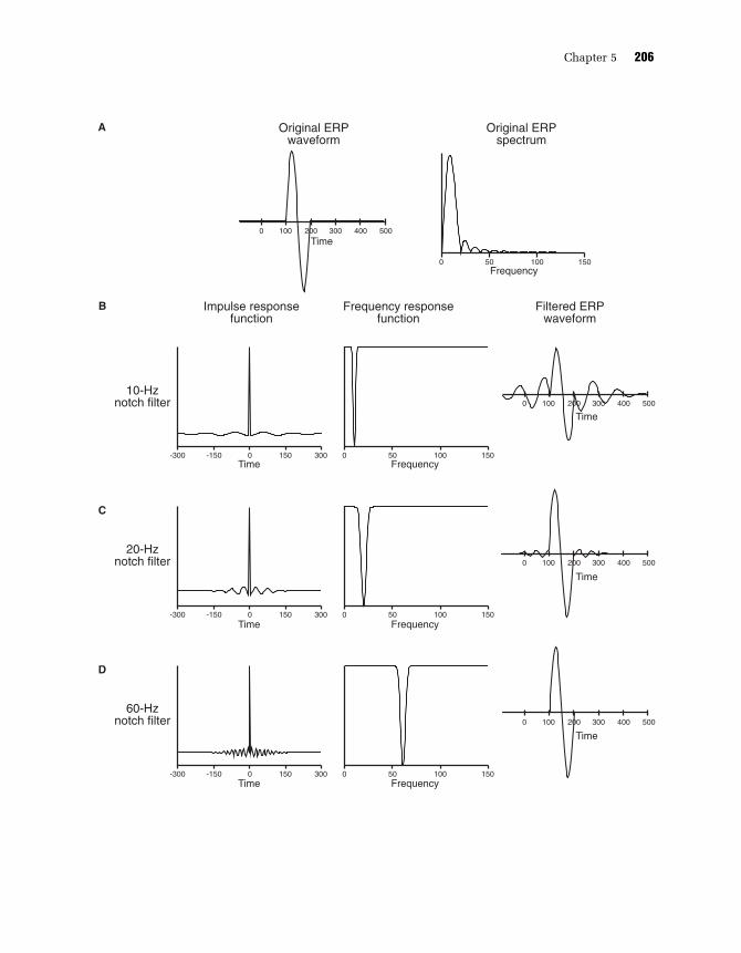
B
A
0 50 100 150-150 150 3000-300
1000 200 300 400 500
0 50 100 150
1000 200 300 400 500
C
D
1000 200 300 400 500
-150 150 3000-300 0 50 100 150
1000 200 300 400 500
-150 150 3000-300 0 50 100 150
Impulse responsefunction
Frequency responsefunction
Filtered ERPwaveform
Original ERPwaveform
Original ERPspectrum
Time
Frequency
Time Frequency
Time
Time Frequency
Time
Time Frequency
Time
60-Hznotch filter
20-Hznotch filter
10-Hznotch filter
Chapter 5 206

The presence of oscillations in the impulse response function is
not alone sufficient to produce large oscillations in the output of
the filter. As figures 5.8C and 5.8D show, notch filters at 20 Hz and
60 Hz produce much smaller oscillations than the 10-Hz notch fil-
ter in the context of this particular artificial ERP waveform. This is
due to the fact that there is much less power at these frequencies in
the spectrum of the unfiltered ERP waveform (see figure 5.8A).
Thus, you must consider both the impulse response function and
the nature of the unfiltered ERP waveform to determine the distor-
tion that a filter will produce.
From these filter-induced distortions, it should be clear that you
must know the shape of the impulse response function to assess
the distortions that a filter might produce. For example, a filter
that is simply labeled ‘‘60-Hz notch filter’’ on an EEG amplifier
will have a very different impulse function from the filter shown
in figure 5.8D, and may lead to much greater distortion of the ERP
waveform than the minimal distortion present in figure 5.8D. Thus,
the common practice of specifying only the half-amplitude or half-
power cutoff of a filter is clearly insufficient; descriptions of filter-
ing should specify the impulse response function in addition to the
cutoff of the filter. For example, when I describe a filter in a journal
article, I write something like this: ‘‘The ERP waveforms were low-
pass filtered offline by convolving them with a Gaussian impulse
response function with a standard deviation of 6 ms and a half-
amplitude cutoff at@30 Hz.’’
Distortions Produced by Low-Pass Filters
In many cases, it is useful to attenuate all frequencies above some
specified point (low-pass filtering). Such filtering is necessary
H Figure 5.8 Examples of temporal distortions produced by notch filters. (A) Shows the originalartificial ERP waveform (one cycle of a 10-Hz sine wave) and its Fourier transform.(B), (C), and (D) show the impulse response and frequency response functions for10-, 20-, and 60-Hz notch filters and also display the result of applying these filtersto the waveform shown in (A).
Filtering 207

during digitization of the raw EEG data, because you must sample
at a rate that is at least twice as high as the highest frequency in the
incoming data. Low-pass filtering is also useful for attenuating the
relatively high-frequency noise caused by muscle activity or by ex-
ternal electrical devices (e.g., line-frequency noise at 50 or 60 Hz).
The cutoff frequency used for a given experiment will depend on
the frequency content of the ERPs being recorded and the fre-
quency content of the noise to be filtered. For example, brainstem
evoked responses contain substantial power at very high frequen-
cies, making a 5-KHz cutoff appropriate, but this makes it difficult
to filter out muscle noise, which falls into the same frequency
range. In contrast, the long-latency ERP components consist
primarily of power under about 30 Hz, making a 30–100 Hz cutoff
appropriate and allowing high-frequency muscle activity to be fil-
tered without much distortion of the underlying ERP waveform.
However, there is almost always some overlap between the fre-
quencies in the ERP waveform and in the noise, and some filter-
induced distortion is therefore inevitable.
This leads us once again to Hansen’s axiom: There is no substi-
tute for good data. Filters necessarily cause distortion, and it is
always better to reduce noise at the source (e.g., through shielding,
low electrode impedance, high common-mode rejection, careful
experimental design, etc.) than to attenuate it with filters. When
you cannot avoid filtering, it is important to choose a filter with an
optimal balance between suppression of noise and distortion of the
ERP waveform. Depending on the nature of the experimental ques-
tion being addressed, some types of distortion may be more prob-
lematic than others, and there are therefore no simple rules for
designing an optimal filter.
Most discussions of filter design emphasize the frequency do-
main and therefore lead to filters such as the windowed ideal filter
shown in figure 5.9A. This particular windowed ideal filter has a
half-amplitude cutoff at 12.5 Hz and is an ‘‘ideal’’ filter because it
perfectly passes all frequencies below approximately 12 Hz and
completely suppresses all frequencies above approximately 13 Hz,
Chapter 5 208

with only a narrow ‘‘transition band’’ in which the attenuation is
incomplete. This filter also produces no phase distortion because
its impulse response function is symmetric around time zero.
Despite the usefulness of these attributes, the sharp transitions
in the frequency response function of this filter require a broad,
oscillating impulse response function, which leads to substantial
distortion in the time domain. This can be seen when this filter is
applied to the artificial ERP waveform from figure 5.8A, yielding
an output containing damped oscillations both before and after the
time range of the original ERP waveform5 (see figure 5.9A, right
column). Importantly, the filtered waveform contains peaks at
around 70 ms and 230 ms that are completely artifactual and are a
consequence of the oscillations in the filter’s impulse response
function. Thus, filters with sharp cutoffs in their frequency re-
sponse functions may lead to large distortions in the apparent
onset and offset of an ERP waveform and to artifactual peaks that
are not present in the original ERP waveform. In other words, a
filter that is ideal in terms of its frequency-domain properties may
be far from ideal in terms of its time-domain properties.
Let us consider briefly how this type of distortion might influ-
ence the interpretation of an ERP experiment. As an example, con-
sider the ERP waveform elicited by a visual stimulus over frontal
cortex, which typically contains an N1 component at about 130
ms but has no prior peaks (the earlier P1 component is typically
absent at frontal sites). If this waveform were filtered with the low-
pass filter shown in figure 5.9A, the filtered waveform would con-
tain an artifactual positive peak preceding the N1 component and
peaking at about 70 ms post-stimulus, and this artifactual peak
might be mistaken for the P1 component. Moreover, if two condi-
tions were compared, one of which produced a larger N1 compo-
nent than the other, these amplitude differences would also be
observed in the artifactual pseudo-P1 component. On the basis of
the filtered response, one might conclude that the experimen-
tal manipulation caused an increase in P1 amplitude at 70 ms
even though there was no real P1 component and the experimental
Filtering 209

B
0 25 50 75-150 150 3000-300
1000 200 300 400 500
C
D
1000 200 300 400 500
-150 150 3000-300 0 25 50 75
1000 200 300 400 500
-150 150 3000-300 0 25 50 75
Impulse responsefunction
A
0 25 50 75
1000 200 300 400 500
-150 150 3000-300
Original
Filtered
Frequency responsefunction
Filtered ERPwaveform
Time Frequency
Time
Time Frequency
Time
Time Frequency
Time
Time Frequency
Time
Win
dow
ed id
eal
filte
rR
unni
ng a
vera
gefil
ter
Gau
ssia
nfil
ter
Sin
gle
pole
caus
al fi
lter
Chapter 5 210

effect did not actually begin until 100 ms. This example under-
scores the necessity of knowing the impulse response function of a
filter to avoid making incorrect conclusions about the time course
of ERP activity.
The bottom three panels of figure 5.9 show several alternative
filters that have approximately the same 12.5-Hz half-amplitude
cutoff frequency as the windowed ideal filter shown in the top
panel, but produce substantially less waveform distortion. The first
of these is a simple running average filter that is equivalent to aver-
aging successive points together (as described in the initial discus-
sion of low-pass filtering). The impulse response function of this
filter extends over a very narrow time range compared to the win-
dowed ideal filter, and therefore causes much less temporal spread
in the filtered ERP waveform. As the right column of figure 5.9B
shows, the output of the running average filter begins slightly be-
fore and ends slightly after the original waveform, but the filter
causes relatively little change in the overall shape of the waveform.
This filter has two shortcomings, however. First, there is substan-
tial attenuation in the 10-Hz frequency band where most of the
power of the original ERP waveform is located, so the filtered
waveform is somewhat smaller than the original. Second, the fre-
quency response function of the filter does not fall monotonically
to zero. Instead, there are side lobes that allow substantial noise
from some high frequencies to remain in the filtered waveform
(this cannot be seen in the examples shown in figure 5.9, which
contain no high-frequency noise). These side lobes can be pre-
dicted from the square shape of the impulse response function:
because the transfer function is the Fourier transform of the im-
pulse response function, the high frequencies required for the
H Figure 5.9 Examples of temporal distortions produced by several types of low-pass filters, eachwith a half-amplitude cutoff of approximately 12.5 Hz. The left and middle columnsshow the impulse and frequency response functions of the filters, respectively. Theright column shows the result of applying each filter to the artificial ERP waveformshown in figure 5.8A.
Filtering 211

sudden onset and offset of the impulse response function lead to
the presence of substantial high frequency power in the frequency
response function.
Figure 5.9C shows a filter with a gaussian impulse response
function that has approximately the same temporal spread as the
running average impulse response function. Like the running aver-
age filter, the gaussian filter produces some smearing in the onset
and offset of the filtered ERP waveform and some attenuation of
the overall waveform. However, the frequency response function
of the gaussian filter falls monotonically to zero, leading to virtu-
ally complete attenuation of frequencies greater than 30 Hz. In
most cases, a gaussian filter provides the best compromise between
the time and frequency domains, with a monotonic and fairly rapid
fall-off in the frequency response function combined with minimal
temporal distortion of the ERP waveform. Typically, a gaussian
filter with a half-amplitude cutoff of 30 Hz will eliminate most
line-frequency and muscle noise while producing very little atten-
uation of the long-latency ERP components and relatively little
latency smearing. In the vast majority of cases, I would recommend
using gaussian impulse response functions for low-pass filtering.
The frequency-domain properties of filters are often described
by a single number, the half-amplitude cutoff frequency. The time-
domain properties of a gaussian filter can also be described with a
single number that reflects the width of the impulse response
function. There are two common ways to do this. First, you can
indicate the standard deviation of the gaussian. Second, you can
indicate how many milliseconds wide the gaussian function is at
half of its maximum value, which is called the full width at half
maximum (FWHM). fMRI experiments commonly use spatial gaus-
sian filters, and FWHM is the usual way of describing the impulse
response function in that context. These values can be intercon-
verted with the filter’s half-amplitude cutoff. The half-amplitude
cutoff in Hz of a gaussian filter with a standard deviation of s milli-
seconds is simply 185:5=s (e.g., a gaussian filter with a standard
deviation of 4 ms would have a half amplitude cutoff of 185:5=4
Chapter 5 212

Hz). The FWHM in milliseconds is equal to 2.355 times the stan-
dard deviation in milliseconds, and the half-amplitude cutoff in
Hz can be computed as 79:62=FWHM.
The windowed ideal, running average, and gaussian filters de-
scribed so far are among the most commonly used low-pass dig-
ital filters for ERP research, and each has certain advantages and
disadvantages. Because of its sharp cutoff, the windowed ideal
function may be appropriate when the ERP waveform and the to-
be-filtered noise contain substantial power in nearby frequency
ranges. However, this filter type leads to substantial distortion in
the time domain, which may lead to incorrect conclusions about
the timing of an ERP component and may even lead to spurious
peaks before the onset or after the offset of the real ERP waveform.
In recordings of long-latency ERP components, the noise is usually
concentrated at substantially higher frequencies than the majority
of the ERP power, making the sharp cutoff of the windowed ideal
filter unnecessary, and a gaussian or running average filter is there-
fore more appropriate. One exception to this occurs when an ERP
waveform is contaminated by alpha-frequency (@ 10 Hz) EEG noise
that interferes with late components such as the P300, which have
their power concentrated at slightly lower frequencies. The best
way to eliminate alpha noise is usually to maintain subject alert-
ness and average together a large number of trials (consistent with
Hansen’s axiom), but this is not always feasible. When necessary, it
is possible to use a windowed ideal filter with a half-amplitude
cutoff frequency of around 8 Hz to attenuate alpha activity, but the
resulting data must be interpreted cautiously because of the time-
domain distortions that such a filter will inevitably produce.
The running average and gaussian filters produce similar pat-
terns of temporal distortion, characterized primarily by the smear-
ing of onset and offset times, but the gaussian filter is usually
preferable because its frequency response function falls to zero at
high frequencies. The running average filter is somewhat easier to
implement, however, which is important in some applications. In
addition, it is sometimes possible to take advantage of the multiple
Filtering 213

zero points in the frequency response function of the running
average filter. If the primary goal of filtering is to attenuate line-
frequency noise, it may be possible to employ a running average
filter where the zero points fall exactly at the line frequency and
its harmonics, producing excellent attenuation of line frequency
noise.
The last class of low-pass filters I will discuss here are called
causal filters and are used in analog filtering devices such as EEG
amplifiers (but can also be implemented digitally). These filters
are labeled causal because they reflect the normal pattern of causa-
tion in which an event at a particular time can influence subse-
quent events but not previous events. More precisely, the impulse
response functions of causal filters have values of zero for times
preceding time zero. Viewed from the opposite temporal perspec-
tive, the output of the filter at a given time point reflects only the
input values at previous time points and not the input values at
subsequent time points. Figure 5.9D shows an example of such a
filter, displaying the impulse response function of a very simple
analog filter. Filters that do not obey the normal pattern of causa-
tion (i.e., because they nonzero values before time zero in their
impulse response functions) are called noncausal filters.
Because their impulse response functions extend only one direc-
tion in time, causal filters produce shifts in peak latency and in off-
set time, which are typically considered negative traits. However,
causal filters may produce relatively little distortion of onset la-
tency, which may provide an advantage over noncausal filters
when onset latency is an important variable (see Woldorff, 1993).
This is not always true of causal filters, however; it depends on a
relatively rapid, monotonically decreasing fall-off from time zero in
the impulse response function, as in the filter shown in figure 5.9D.
The frequency response function of the causal filter shown in
figure 5.9D is suboptimal for most purposes because it falls rela-
tively slowly and never reaches zero. This is not an inherent prop-
erty of causal filters, however. For example, if the gaussian impulse
response function shown in figure 5.9C were simply shifted to the
Chapter 5 214

right so that all values were zero prior to time zero, the resulting
causal filter would have the same frequency response function as
the noncausal gaussian filter, but the output waveform would be
shifted in time by the same amount as the shift in the impulse
response function. Bessel filters, which can be implemented in
analog circuitry, have an impulse response function that approxi-
mates a shifted gaussian and therefore make an excellent choice
for on-line filtering (e.g., during EEG digitization). Bessel filters
also have a linear phase response, which means that all fre-
quencies in the output waveform are shifted by the same amount
of time. This time shift can be computed and the filtered waveform
can be shifted backwards by this amount off-line, thus eliminating
the latency shifts inherent in analog filters. Unfortunately, Bessel
filters are expensive to implement in analog circuitry, so they are
relatively uncommon.
Some Important Properties of Convolution
Before going further, it is useful to discuss some important
mathematical properties of the convolution operation. In particu-
lar, convolution has the same commutative, associative, and dis-
tributive properties as multiplication. The commutative property
states that it doesn’t matter which of two functions comes first in a
convolution formula. More precisely:
A B ¼ B A
The associative property states that multiple consecutive con-
volutions can be performed in any order. More precisely:
A ðB CÞ ¼ ðA BÞ C
The distributive property states that the convolution of some
function A with the sum of two other functions B and C is equal to
A convolved with B plus A convolved with C. More precisely:
A ðBþ CÞ ¼ ðA BÞ þ ðA CÞ
Filtering 215

These mathematical properties of convolution lead to several
important properties of filters. For example, one common question
about filtering is: what happens when you filter a filtered waveform
a second time? If we have two filters with impulse response func-
tions denoted by IRF1 and IRF2 and an ERP waveform denoted by
ERP, we can write the process of filtering twice as:
ðERP IRF1Þ IRF2
Because of the associative property, this is equal to convolving
the two impulse response functions first and then convolving the
result with the ERP waveform:
ERP ðIRF1 IRF2Þ
To take a concrete example, the convolution of two gaussian
functions yields a somewhat wider gaussian, and filtering an ERP
twice with a gaussian filter is therefore equivalent to filtering once
with a wider gaussian.
In addition, because convolution in the time domain is equiva-
lent to multiplication in the frequency domain, the frequency re-
sponse function of the double filtering is equal to the product of
the frequency response functions of the two individual filters. In
the case of two gaussian filters, this would lead to greater attenua-
tion of high frequencies than either filter would produce alone. In
the more common case of the application of both a low-pass filter
and a high-pass filter, the result is a band-pass filter that simply
cuts both the high and low frequencies. However, if both filters
have relatively gradual frequency response functions, the multipli-
cation of these functions may also lead to fairly substantial attenu-
ation of the intermediate frequencies.
Time-Domain Implementation of High-Pass Filters
In the initial discussion of high-pass filters near the beginning of
the chapter, I mentioned that one can accomplish high-pass filter-
ing by creating a low-pass-filtered waveform and subtracting this
Chapter 5 216

from the unfiltered waveform, thus yielding the high frequencies
that are present in the unfiltered waveform and absent in the low-
pass-filtered waveform. This process can be expressed as:
ERPH ¼ ERP ERPL ¼ ERP ðIRFL ERPÞ
where ERPH and ERPL are the high- and low-pass-filtered ERP
waveforms and IRFL is the impulse response function of the
low-pass filter. This convolution-and-subtraction sequence can be
replaced by a single convolution with a high-pass impulse re-
sponse function that can be computed by some simple algebraic
manipulations. First, it is necessary to define a ‘‘unity’’ impulse
response function IRFU that is 1.0 at time zero and 0.0 at all other
points; the convolution of this function with an ERP waveform
would be equal to the ERP waveform (analogous to the multiplica-
tion of a number by 1.0). By using this unity function, we can use
the distributive property to create an impulse response function
IRFH that will accomplish high-pass filtering in a single step:
ERPH ¼ ERP ðIRFL ERPÞ
¼ ðIRFU ERPÞ ðIRFL ERPÞ ½because ERP ¼ IRFU ERP
¼ ðIRFU IRFLÞ ERP ½because of the distributive property
¼ IRFH ERP; where IRFH ¼ IRFU IRFL
Thus, we can create a high-pass impulse response function by
subtracting a low-pass impulse response function from the unity
impulse response function ðIRFU IRFLÞ. The frequency response
function of the resulting high-pass filter is simply the complement
of the frequency response function of the low-pass filter (1.0 minus
the response at each individual frequency point in the low-pass
frequency response function).
Figure 5.10A diagrams the creation of a high-pass impulse
response function from a unity impulse response function and
a gaussian low-pass impulse response function with a half-
amplitude cutoff of 2.5 Hz. The unity impulse response function
(figure 5.10A, left) consists of a single spike of magnitude 1.0 at
Filtering 217

B
0 25 50 75
A
-150 150 3000-300 -150 150 3000-300
Unityimpulse response
function
-150 150 3000-300
1000 200 300 400 500 600 1000 200 300 400 500 600
OriginalERP waveform
C
0 25 50 75
1000 200 300 400 500 600 1000 200 300 400 500 600
D
0 25 50 75
1000 200 300 400 500 600 1000 200 300 400 500 600
Gaussian low-passimpulse response
function
Gaussian high-passimpulse response
function
OriginalERP spectrum
FilteredERP waveform
Time
Frequency
Time Time
Time Time
Frequency
Time Time
Frequency
Time Time
Chapter 5 218

time zero, which is very large compared to the values at individual
time points in the gaussian low-pass impulse response function
(figure 5.10A, middle). The high-pass impulse response function is
created by simply subtracting the low-pass impulse response func-
tion from the unity function, as shown at the right of figure 5.10A.
A related attribute of the class of filters discussed here is that
they are linear, so you can combine filtering with other linear oper-
ations in any order. For example, signal averaging is also a linear
process, and this means that filtering an averaged ERP waveform
yields the same result as filtering the EEG data before averaging.6
Averaged ERP data sets are typically considerably smaller than the
EEG data from which they are derived, and filtering after averaging
is therefore more efficient than filtering the raw EEG and then
averaging.
Distortions Produced by High-Pass Filters
Figure 5.10 shows the application of a gaussian high-pass filter to
two artificial ERP waveforms and one realistic ERP waveform. The
inverted gaussian in the impulse response function is visible in the
filtered ERP waveforms, where it produces overshoots that one can
observe at the beginning and end of the waveforms. These distor-
tions are particularly evident for ERP waveforms that consist pri-
marily of one polarity, such as those in figures 5.10C and 5.10D.
This can be understood by viewing filtering as replacing each sam-
ple in the ERP waveform with a scaled copy of the impulse
response function: when the unfiltered ERP waveform consists of
roughly equivalent positive and negative subcomponents, as in
figure 5.10B, these subcomponents will lead to opposite-polarity
copies of the impulse response function, which will cancel each
H Figure 5.10 Construction and application of a gaussian high-pass filter. (A) A unity impulseresponse function multiplied by a gaussian low-pass impulse response functionyields a gaussian high-pass impulse response function. (B), (C), and (D) show theapplication of this filter to three different ERP waveforms.
Filtering 219

other out to some extent. The amount of cancellation will depend
on the exact shapes of the waveform and the impulse response
function, but in most cases the overshoot will be greater when one
polarity dominates the ERP waveform.
The distortions in figure 5.10 are in some sense similar to the
distortions the gaussian low-pass filter shown in figure 5.9C pro-
duced, but reversed in polarity because the gaussian in the high-
pass impulse response function is inverted (because of the lower
cutoff frequency of the high-pass filter, the distortion in figure 5.10
is also somewhat broader than the distortion in figure 5.9C). Thus,
when an ERP waveform is low-pass filtered, the gaussian impulse
response function produces a spreading of the peaks that is the
same polarity as the peaks, whereas using a high-pass filter
produces opposite-polarity spreading. Although these distortions
are similar in many ways, the distortions the high-pass filter pro-
duces may be more problematic because they may lead to the ap-
pearance of artifactual peaks, such as the peaks at approximately
75 ms and 450 ms in the filtered waveform shown in figure 5.10D.
Figure 5.11 shows the effects of several different types of high-
pass filters (all with half-amplitude cutoffs at approximately 2.5
Hz) on a realistic ERP waveform. Although the impulse response
and frequency response functions of the windowed ideal and gaus-
sian filters (panels A and B) look very similar, the windowed ideal
impulse response function contains damped oscillations just like
those in the windowed ideal low-pass filter in figure 5.9A. The
half-amplitude cutoff frequency of the high-pass filter shown here
is so low, however, that these oscillations fall outside of the plotted
time window; with a higher cutoff frequency, these oscillations
would be more apparent. Thus, windowed ideal high-pass filters
may induce artificial oscillations in the filtered ERP waveform,
whereas gaussian high-pass filters do not. As discussed above and
shown in figure 5.11B, however, gaussian high-pass filters can
produce individual artifactual peaks at the beginning and end of
the filtered waveform, unlike gaussian low-pass filters. For this
reason, you must take extreme caution in interpreting high-pass-
Chapter 5 220

B
0 5 10 15-150 150 3000-300
C
D
-150 150 3000-300 0 5 10 15
-150 150 3000-300 0 5 10 15
A
0 5 10 15-150 150 3000-300
1000 200 300 400 500 600
1000 200 300 400 500 600
1000 200 300 400 500 600
1000 200 300 400 500 600
Impulse responsefunction
Frequency responsefunction
ERP waveforms
Original
Filtered
FrequencyTime
Time
FrequencyTime
Time
FrequencyTime
Time
FrequencyTime
Time
Win
dow
ed id
eal
filte
rG
auss
ian
filte
rS
ingl
e po
leca
usal
filte
rH
alf-
gaus
sian
caus
al fi
lter
Figure 5.11 Application of four different high-pass filters to a sample ERP waveform. All have a50 percent amplitude cutoff near 2.5 Hz.
Filtering 221

filtered waveforms, even when using a gaussian impulse response
function.
Figure 5.11C shows the impulse response and frequency re-
sponse functions of the type of causal filter found in older EEG
amplifiers. Because its impulse response function is zero for all
points before time zero, this filter cannot produce any distortion
before the onset of the unfiltered ERP waveform and thus does not
produce an artifactual peak at the beginning of the filtered ERP
waveform. However, this same attribute of causal filters leads to
distorted peak latencies in the filtered waveform, whereas this
form of distortion is absent for most noncausal filters. These differ-
ent forms of distortion underscore the important principle that all
filters produce distortions, and the choice of which filter to use
will depend upon the goals of the experiment and the types of
distortion that are acceptable. The filter shown in figure 5.11C also
has a relatively gradual roll-off; this can be improved by using the
filter in figure 5.11D, which uses the right half of a gaussian in its
impulse response function. Like the filter in figure 5.11C, this
‘‘half-gaussian’’ filter produces minimal distortion at the beginning
of the filter ERP waveform, but has a somewhat sharper roll-off and
is therefore a better choice in many cases.
In most cases, noncausal high-pass filters tend to take low-
frequency information away from the time zone of the unfiltered
ERP waveform and ‘‘push’’ it forward and backward in time in the
filtered ERP waveform. In contrast, causal high-pass filters of the
type shown in figure 5.11 push the information exclusively to later
time points. Figure 5.12 illustrates this. ERP waveforms typically
consist of small, relatively high-frequency early components fol-
lowed by larger, relatively low-frequency late components, and
this asymmetrical sequence makes the bidirectional distortions
produced by noncausal high-pass filters particularly harmful.
In particular, low frequency information from the large, low-
frequency later components is pushed into the latency range of the
smaller early components, causing substantial distortion of the
early components even though they contain relatively little low-
Chapter 5 222

frequency information. Using a causal filter such as those shown in
panels C and D of figure 5.11, however, will minimize distortion of
the early components because low-frequency information from the
late components will not be pushed backward into the time range
of the early components. Note, however, that this is true only for
filters that have monotonically increasing impulse response func-
tions after time zero; filters that do not possess this property, such
as Bessel filters, may cause distortions similar to those produced
by noncausal filters. In addition, causal filters may produce sub-
stantial latency shifts that may be problematic in some cases.
Recommendations Revisited
I discussed some recommendations about filtering early in this
chapter. Now that you have a deeper understanding of how filters
actually work, you might want to read through those recommenda-
tions again.
Noncausal gaussianhigh-pass filter
Causal half-gaussianhigh-pass filter
LatencyShift
Time100 200 300 400 5000 600 100 200 300 400 5000 600
Low frequencyinformation pushedbackward in time
Low frequencyinformation pushed
forward in time
Low frequencyinformation pushed
forward in time
Time
Figure 5.12 Comparison of a noncausal gaussian high-pass filter and a causal half-gaussianhigh-pass filter. Note that the noncausal filter produces obvious distortions at thebeginning and end of the waveform, whereas the causal filter produces no distortionat the beginning of the waveform. Note also that the causal filter produces a largelatency shift, but the noncausal filter does not.
Filtering 223

My two most important recommendations are as follows.
First, filter the data as little as possible. As you’ve seen, filters
always distort the time-domain properties of ERP waveforms, and
you don’t want to distort your waveforms unnecessarily. My sec-
ond main recommendation is that before you use a filter, think
about exactly how it might distort your data. Often, the best way
to see how a filter will distort your data is to create a simulated,
noise-free waveform and apply the filter to it. This will allow you
to see how the filter distorts component onsets and offsets and
adds spurious components or oscillations to your data. If the
effects of the filter on the simulated data aren’t too bad, then you
can use the filter on your real data with confidence that the filter
will help you rather than hurt you.
Chapter 5 224

6 Plotting, Measurement, and Analysis
The previous chapters have discussed designing experiments, col-
lecting the data, and applying signal processing procedures; this
chapter discusses the final steps in an ERP experiment: plotting the
data, measuring the components, and subjecting these measure-
ments to statistical analyses.
Plotting ERP Data
Although it might seem trivial to plot ERP waveforms, I regularly
read ERP papers in which the waveforms are plotted in a way that
makes it difficult to perceive the key aspects of the waveforms.
Thus, I will begin this chapter with a few recommendations about
plotting ERP data.
The most important thing to keep in mind is that virtually all
ERP papers should include plots of the key ERP waveforms. Given
all of the difficulties involved in isolating specific ERP com-
ponents, it is absolutely necessary to see the waveforms before
accepting the validity of a paper’s conclusions. Remember that
Kramer (1985) showed that ERP experts do a good job of determin-
ing the underlying latent components when they see the observed
ERP waveforms, and presenting the waveforms is essential for
this. In fact, the official publication guidelines of the Society for
Psychophysiological Research (SPR) state that ‘‘the presentation of
averaged ERP waveforms that illustrate the principal phenomena
being reported is mandatory’’ (Picton et al., 2000, p. 139).
The SPR guidelines describe several additional elements of ERP
figures that you should keep in mind. First, it is almost always a
good idea to show the data from multiple electrode sites, spanning

the region of the scalp where the effects of interest were present.
This information plays a key role in allowing experts to deter-
mine the underlying component structure of the waveform. How-
ever, including multiple electrode sites is not as important when
you can isolate components by other means (e.g., by performing
the subtraction procedure that isolates the lateralized readiness
potential).
Second, plots of ERP waveforms should indicate the voltage
scale and the time scale in a way that makes it easy for readers to
assess amplitudes and latencies. The voltage scale should indicate
whether positive or negative is up (and if negative is up, I would
recommend stating this in the figure caption). In addition, the elec-
trode sites should be labeled in the figure (if a single site is shown,
I often indicate the site in the caption).
Figure 6.1 shows an example of a bad way (panel A) and a good
way (panel B) to plot ERP waveforms. The most egregious error in
200 ms
5µV
200-200
–5µV
+5µV 400 600 800
Frequent
Frequent Rare
Rare
Cz
A
B
Figure 6.1 Examples of a poor way to plot ERP waveforms (A) and a good way to plot them (B).Negative is plotted upward.
Chapter 6 226

panel A is that there is no X axis line running through zero micro-
volts to provide an anchor point for the waveforms. It is absolutely
essential to include an X axis line that shows the zero microvolt
point and the time scale for each waveform. Without it, the reader
will find it difficult to determine the amplitude or the latency of
the various points in the waveform. A separate scale marker, such
as that shown in figure 6.1A, is not enough, because it does not
provide a visual reference point. For example, can you tell how
much bigger the first component is in the left waveform than in
the right waveform? And can you see that this component peaks
earlier in the right waveform than in the left waveform?
The second most egregious error in figure 6.1A is that the wave-
forms are not overlapped. This makes it very difficult for the reader
to determine the exact pattern of effects. For example, can you
tell exactly when the difference between the waveforms switches
polarities? All key effects should be shown by overlapping the rel-
evant waveforms. Figure 6.1A also fails to indicate time zero, and
it is impossible to tell which polarity is plotted upward.
Panel B of figure 6.1 solves these problems. It has an X axis run-
ning through the waveforms, which are overlapped. It provides ad-
ditional calibration axis, indicating the latencies (with minor tick
marks as well, showing the intermediate latencies). The voltage
calibration indicates the polarity of the waveform. The two wave-
forms are drawn in easy-to-distinguish line types, and the figure
provides a legend to indicate what condition each line type repre-
sents (this is much better than providing this information in words
in the figure caption or main text). The figure also indicates the
electrode site at which the waveforms were measured.
It is also essential for the plot to show a significant presti-
mulus portion of the waveforms. The prestimulus period allows
the reader to assess the overall noise level of the recordings and
the presence of overlap from the preceding trials. In addition, the
apparent amplitude of the ERP peaks will depend on the baseline
level, and a stable baseline is therefore essential for accurately
characterizing the differences between two or more waveforms.
Plotting, Measurement, and Analysis 227

I almost always provide a 200-ms prestimulus baseline, and I
would recommend this for the vast majority of cognitive ERP
experiments.
You should be careful when selecting the line types for the ERP
waveforms. First, you need to use reasonably thick lines. Figures
are usually reduced by a factor of two or three times for publica-
tion, making lines that were originally moderately thin become so
thin that they are nearly invisible. If someone makes a photocopy
of the journal article, portions of the lines may disappear. Of
course, you don’t want to make the lines so thick that they obscure
the experimental effects. I find that a two-point width works well
in the majority of cases. In addition, when multiple waveforms
overlap, you should make sure that the different lines are easy to
differentiate. The best way to do this is with solid, dashed, and
dotted lines (or with color, if available, but then photocopies will
lose the information). You should avoid using different line thick-
nesses to differentiate the waveforms; this doesn’t work as well,
and the thin lines may disappear once the figure has been reduced
for publication. In general, you should avoid overlapping more
than three waveforms (four if absolutely necessary). With more
overlapping waveforms, the figure starts to look like spaghetti.
How many different electrode sites should you show? This
depends, in part, on the expected audience. If the paper will be
published in an ERP-oriented journal, such as Psychophysiology,
the readers will expect to see waveforms from a broad selection of
electrode sites. If the paper will be published in a journal where
ERP studies are not terribly common, such as Journal of Neuro-
science or JEP: General, you should show only the key sites. If you
have recorded from a large number of electrodes, it is pointless to
include a figure showing the data from all the sites. If a figure con-
tains more than ten to fifteen sites, the individual waveforms will
be so small that they will provide very little information. It is
much better to show a representative sample of the electrode sites
and then use topographic maps to show the distribution of voltage
over the scalp.
Chapter 6 228

Measuring ERP Amplitudes
Most ERP studies concentrate on the amplitudes of one or more
ERP components, and it is important to measure amplitude accu-
rately. As figure 6.2 illustrates, there are two common ways to mea-
sure ERP amplitudes. The most common method is to define a time
window and, for each waveform being measured, find the maxi-
mum amplitude in that time window. This is called a peak ampli-
tude measure. The second most common method is to define a
time window and, for each waveform being measured, calculate
the mean voltage in that time window. This is called a mean am-
plitude measure. It is also possible to calculate the sum of the vol-
tages at each time point within the measurement window (an area
-5 µV
-200 200 400 600+5 µV
P1
N1
P2
P3
N2
Maximum Voltage
Maximum Voltage
MeasurementWindow
Local Peak
Local Peak
Area/Mean
A
B
C
Figure 6.2 (A) ERP waveform with several peaks. (B) ERP waveform, with a measurementwindow from 150–300 ms poststimulus and several measures. (C) Filtered ERPwaveform. Negative is plotted upward.
Plotting, Measurement, and Analysis 229
amplitude measure), but this is really just the mean amplitude
multiplied by the number of points in the measurement window.
For all of these measures, the voltages are typically measured rela-
tive to the average voltage in the prestimulus period. Other tech-
niques are sometimes used, but they are beyond the scope of this
book.
The goal of these techniques is to provide an accurate measure-
ment of the size of the underlying ERP component with minimal
distortion from noise and from other, overlapping components. As
I discussed at the beginning of chapter 2, it is very difficult to mea-
sure the amplitude and latency directly from a raw ERP waveform
without distortion from overlapping components. That chapter
also described several strategies for avoiding this problem (e.g., us-
ing difference waves), but those strategies often rely on the use of
an appropriate measurement approach. And don’t forget rule 1
from chapter 2: Peaks and components are not the same thing.
There is nothing special about the point at which the voltage
reaches a local maximum.
Peak Amplitude
Given that the point at which the voltage reaches a local maximum
is not special, why should you use peak amplitude to measure
the amplitude of an ERP component? In fact, there is no compel-
ling reason to use peak amplitude measures in most ERP experi-
ments (although there might be good reasons to use this measure
in some special cases). Moreover, there are several reasons why
you shouldn’t use peak amplitude in many cases, at least not with-
out some modifications to the basic procedure.
Consider, for example, the ERP waveform shown in panel A of
figure 6.2. To measure the peak of the P2 wave, you might use a
time window of 150–300 ms. As panel B of figure 6.2 shows, the
maximum voltage in this time window occurs at the edge of the
time window (300 ms) due to the onset of the P3 wave. Conse-
quently, the amplitude of the P2 wave would be measured at 300
Chapter 6 230

ms, which is not very near the actual P2 peak. Clearly, this is not a
good way to measure the P2 wave. You could avoid this problem
by using a narrower measurement window, but a fairly wide win-
dow is usually necessary because of variations in peak latency
across electrode sites, experimental conditions, and subjects. A
much better way to avoid this problem is to search the measure-
ment window for the largest point that is surrounded on both sides
by smaller points. I call this measure local peak amplitude, and
I refer to the original method as simple peak amplitude. To
minimize spurious local peaks caused by high-frequency noise,
the local peak should be defined as having a greater voltage than
the average of the three to five points on either side rather than the
one point on either side.1
Local peak amplitude is obviously a better measure than the
simple peak amplitude. Strangely, I have never seen anyone
explicitly describe this way of measuring peaks. It may be that
people use it and just call it peak amplitude (I have done this my-
self), but it would probably be best if everyone used the term local
peak amplitude to make it clear exactly how the peaks were
measured.
Although local peak amplitude is a better measure than the sim-
ple peak amplitude, high-frequency noise can significantly distort
both of these measures. In figure 6.2B, for example, the local peak
is not in the center of the P2 wave, but is shifted to the right be-
cause of a noise deflection. It makes sense that peak amplitude
would tend to be noise-prone, because the voltage at a single time
point is used to measure a component that lasts for hundreds of
milliseconds. Moreover, the peak amplitude measurements will
tend to be larger for noisier data and for wider measurement win-
dows, because both of these factors increase the likelihood that a
really large noise deflection will occur by chance. Consequently, it
is never valid to compare peak amplitudes from averages of differ-
ent numbers of trials or from time windows of different lengths. I
have seen this rule violated in several ERP papers, and it definitely
biases the results.
Plotting, Measurement, and Analysis 231

If, for some reason, you still want to measure peak amplitude,
you can reduce the effects of high-frequency noise by filtering out
the high frequencies before measuring the peak. Panel C of figure
6.2, which shows the waveform in panels B and C after low-pass
filtering, illustrates this. In the filtered waveform, the simple peak
amplitude again provides a distorted measure, but the local peak
provides a reasonably good measure of the amplitude. As dis-
cussed in chapter 5, when high frequencies are filtered out, the
voltage at each point in the filtered waveform reflects a weighted
contribution of the voltages from the nearby time points. Thus, the
peak amplitude in a filtered waveform avoids the problem of using
the voltage at a single time point to represent a component that
lasts hundreds of milliseconds.
Another shortcoming of peak amplitude measures is that they
are essentially nonlinear. For example, if you measure the peak
amplitude of the P2 wave for several subjects and compute the av-
erage of the peak amplitudes, the result will almost always be dif-
ferent from what would you would get by creating a grand average
of the single-subject waveforms and measuring the peak amplitude
of the P2 wave in this grand average. This may cause a discrepancy
between the grand-average waveforms that you present in your
figures and the averaged peak amplitude values that you analyze
statistically. Similarly, when there is variability in the latency of
a component from trial to trial in the raw EEG data, the peak ampli-
tude in the averaged ERP waveform will be smaller than the single-
trial amplitudes (see panels G and H of figure 2.1 in chapter 2). If
latency variability is greater in one condition than in another, the
peak amplitudes will differ between conditions even if there is no
difference between conditions in the single-trial peak amplitudes.
To summarize, peak amplitude measures have four serious
shortcomings: (1) when the maximum voltage in the measurement
window is measured, the rising or falling edge of an overlapping
component at the border of the measurement window may be
measured rather than the desired peak; (2) peak amplitude uses a
Chapter 6 232
single point to represent a component that may last hundreds of
milliseconds, making it sensitive to noise; (3) peak amplitude will
be artificially increased if the noise level is higher (due, for exam-
ple, to a smaller number of trials) or if the measurement interval is
longer; (4) peak amplitude is a nonlinear measure that may not cor-
respond well with grand-average ERP waveforms or with single-
trial peaks.
It might be tempting to argue that peak amplitude is a useful
measure because it takes into account variations in latency among
conditions, electrode sites, and subjects. After all, you wouldn’t
want to measure the amplitude of a component at the same time
point at all electrode sites if the component peaks later at some
sites than at others, would you? This argument is fallacious and
points to a more abstract reason for avoiding peak amplitude mea-
sures. Specifically, peak amplitude measures implicitly encourage
the mistaken view that peaks and components are the same thing
and that there is something special about the point at which the
voltage reaches its maximum value.
For example, the fact that the voltage reaches its maximum value
at different times for different electrode sites is unlikely to reflect
differences in the latency of the underlying component at different
electrode sites. A component, as typically defined, is a single brain
process that influences the recorded voltage simultaneously at all
electrode sites, and it cannot have a different latency at different
sites. As described in chapter 2 (see especially figure 2.1), the tim-
ing of a peak in the observed ERP waveform will vary as a function
of the relative amplitudes of the various overlapping components,
and this is the reason why peak latencies vary across electrode
sites. Indeed, it would be rather strange to measure the same com-
ponent at different times for the different electrode sites. Similarly,
peak latency differences between subjects are just as likely to be
due to differences in the relative amplitudes of the various under-
lying components as differences in the latency of the component
of interest. In contrast, the latency of the underlying component
Plotting, Measurement, and Analysis 233

may indeed vary considerably across different experimental condi-
tions. But in this case, it will be nearly impossible to measure the
component without significant distortion from other overlapping
components, because amplitude and latency measures are often
confounded (see chapter 2). Thus, although peak amplitude mea-
sures might seem less influenced by changes in component timing,
this is really an illusory advantage.
Mean Amplitude
Mean amplitude has several advantages over peak amplitude. First,
you can use a narrower measurement window because it doesn’t
matter if the maximum amplitude falls outside of this window
for some electrode sites or some subjects. In fact, the narrower
the window, the less influence overlapping components will have
on the measurements. As an example, a measurement window of
200–250 ms would be appropriate for measuring the mean ampli-
tude of the P2 component in the waveform shown in figure 6.2,
compared to a window of 150–300 ms that would be appropriate
for a peak amplitude measure.
A second advantage of mean amplitude measures is that they
tend to be less sensitive to high-frequency noise than are peak am-
plitude measures, because a range of time points is used rather
than a single time point. For this reason, you don’t want to make
your measurement windows too narrow (< 40 ms or so), even
though a narrow window is useful for mitigating the effects of over-
lapping components. You should also note that, although filtering
can reduce the effects of high-frequency noise in peak amplitude
measures, there is no advantage to low-pass filtering when measur-
ing mean amplitude. By definition, mean amplitude includes the
voltages from multiple nearby time points, and this is exactly
what low-pass filtering does. In fact, filtering the data before mea-
suring the mean amplitude in a given measurement window is the
same thing as measuring the mean amplitude from an unfiltered
waveform using a wider measurement window.
Chapter 6 234

A third advantage of mean amplitude measures is that they
do not become biased when the noise level increases or when
one uses a longer measurement window. In other words, the
variance may change, but the expected value is independent of
these factors. Consequently, it is legitimate to compare mean am-
plitude measurements from waveforms based on different num-
bers of trials, whereas this is not legitimate for peak amplitude
measurements.
A fourth advantage is that mean amplitude is a linear measure.
That is, if you measure the mean amplitude of a component from
each subject, the mean of these measures will be equal to measur-
ing the mean amplitude of the component from the grand-average
waveform. This makes it possible for you to compare directly
your grand-average waveforms with the means from your statis-
tical analyses. This same principle also applies to the process
of averaging together the single-trial EEG data to form averaged
ERP waveforms. That is, the mean amplitude measured from a
subject’s averaged ERP waveform will be the same as the aver-
age of the mean amplitudes measured from the single-trial EEG
data.
Although mean amplitude has several advantages over peak am-
plitude, it is not a panacea. In particular, mean amplitude is still
quite sensitive to the problem of overlapping components and can
lead to spurious results if the latency of a component varies across
conditions. In addition, there is not always an a priori reason to se-
lect a particular measurement window, and this can encourage
fishing for significant results by trying different windows. There
are some more sophisticated ways of measuring the amplitude of a
component (e.g., dipole source modeling, ICA, PCA, etc.), but these
methods are based on a variety of difficult-to-assess assumptions
and are beyond the scope of this book (for more information on al-
ternative measures, see Coles et al., 1986). Thus, I would generally
recommend using mean amplitude measures in conjunction with
the rules and strategies for avoiding the problem of overlapping
components discussed in chapter 2.
Plotting, Measurement, and Analysis 235

Baselines
Whether you are measuring mean amplitude or peak amplitude, you
will be implicitly or explicitly subtracting a voltage—usually the
average prestimulus voltage—that represents the baseline or zero
point. Any noise in the baseline will therefore add noise to your
measures, so it is important to select an appropriate baseline. When
you are measuring stimulus-locked averages, I would recommend
that you use the average voltage in the 200 ms before stimulus onset
as the baseline. A 100-ms baseline is common, and although it’s
not as good as 200 ms, it’s usually acceptable. If you use less than
100 ms, it is likely that you will be adding noise to your measures.
The prestimulus interval is usually used as the baseline because
it is assumed that the voltage in this period is unaffected by the
stimulus. Although it is true that the time-locking stimulus cannot
influence the prestimulus period, it is important to realize that the
processing does not always begin after the onset of a stimulus. If
the interval between stimuli is relatively short (< 2 s), the late
potentials from the previous stimulus may not have completely
diminished by the time of the time-locking stimulus and may
therefore contribute to the baseline voltage. In addition, regardless
of the length of the interstimulus interval, the prestimulus voltage
may be influenced by preparatory processes (in fact, the effects of
preparatory processes are more visible when the interstimulus in-
terval is long). For these reasons, the prestimulus baseline rarely
provides a perfectly neutral baseline, and in many experiments it
is clear that the voltage slopes upward or downward during the
prestimulus interval because of these factors. This can be a major
problem if the prestimulus activity differs across experimental con-
ditions, because any difference in measured amplitudes between
conditions might reflect prestimulus differences rather than post-
stimulus differences (see chapter 4, and Woldorff, 1988).
Even when the prestimulus activity does not differ across condi-
tions, it is important to recognize that the prestimulus interval is
usually not completely neutral. For example, scalp distributions
can be significantly distorted if significant activity is present in the
Chapter 6 236

prestimulus interval and then fades by the time of the component
being measured. The only real solution is to keep in mind that the
measured voltage reflects the difference between the amplitude in
the measurement window and the amplitude in the prestimulus
period (just as it also reflects the difference between the active and
reference electrodes).
Baselines become much more complicated when using response-
locked averages, because the activity that precedes the response is
often as large as or larger than the activity that follows the re-
sponse. One solution to this problem is to use as the baseline a pe-
riod of time that precedes the response by enough so that it always
precedes the stimulus. Another solution is to use the average volt-
age of the entire averaging epoch as the baseline. As far as I am
aware, there is no single best solution, other than thinking care-
fully about whatever baseline period you use to make sure that it
isn’t distorting your results.
I should also mention that investigators sometimes compute
peak-to-peak amplitudes that consist of the difference in amplitude
between two successive peaks of opposite polarity. For example,
the amplitude of the visual N1 wave is sometimes measured as the
difference in amplitude between the N1 peak and the preceding P1
peak (this could also be done with mean amplitudes, although this
is much less common). This approach is sometimes taken if the
components are assumed to overlap in time such that the earlier
component distorts the amplitude of the later component. This
may be a reasonable approach, as long as you keep in mind exactly
what you are measuring.
Measuring ERP Latencies
Peak Latency
ERP latencies are usually measured with peak latency measures
that find the maximum amplitude within a time window and use
Plotting, Measurement, and Analysis 237
the latency of this peak as a measure of the latency of the underly-
ing component. All of the shortcomings of peak amplitude mea-
sures also have analogs in peak latency measures. First, when the
measurement window includes the rising or falling edge of a larger
component, the maximum voltage will be at the border of the win-
dow (see figure 6.2B). Fortunately, this problem can be solved by
using a local peak latency measure in which a point is not consid-
ered a peak unless the three to five points on each side of it have
smaller values.
A second shortcoming of peak latency measures is that, like peak
amplitude measures, they are highly sensitive to high-frequency
noise. If a peak is rather broad and flat, high-frequency noise may
cause the maximum voltage to be very far away from the middle
of the peak (see the local peak in figure 6.2B). In fact, this is proba-
bly an even more significant problem for peak latency than for
peak amplitude, because a noise-related peak may be far in time
from the true peak but close to the true peak’s amplitude. As in
the case of peak amplitude, you can mitigate this problem to some
extent by filtering out the high frequencies in the waveform (see
the local peak in figure 6.2C).
A third shortcoming is that peak latency, like peak amplitude,
will change systematically as noise levels increase. Specifically, as
the noise increases, the average peak latency will tend to be nearer
to the center of the measurement window. To understand why this
is true, imagine an ERP waveform that is entirely composed of ran-
dom noise. If you measure the peak latency between 200 and 400
ms, the peak latency on any given trial is equally likely to be at
any value in this range, and the average will therefore be at the
center of the range. If there is a signal as well as noise, then the av-
erage will tend to be somewhere between the actual peak and the
center of the range.
A fourth shortcoming of peak latency is that it is nonlinear. In
other words, the peak latency measured from a grand average
will not usually be the same as the average of the peak latencies
that were measured from the single-subject waveforms. Similarly,
Chapter 6 238

the peak latency measured from a single-subject average will
not usually be the same as the average of the single-trial peak
latencies.
A fifth shortcoming is that peak latency measures, like peak am-
plitudemeasures, implicitly encourage themistaken view that peaks
and components are the same thing and that there is something
special about the point at which the voltage reaches its maximum
value. The latency at which the voltage reaches its maximum value
depends greatly on the nature of the overlapping components and
the waveshape of the component of interest, so peak latency bears
no special relationship to the timing of an ERP component.
Although peak latency has many shortcomings, there just aren’t
many good alternatives, and so it is often the best measure. When
measuring peak latency, you should take the following precau-
tions: (1) filter out the high-frequency noise in the waveforms; (2)
use a local peak measure rather than an absolute peak measure; (3)
make sure that the waveforms being compared have similar noise
levels; and (4) keep in mind that peak latency is a coarse and non-
linear measure of a component’s timing.
Fractional Area Latency
Under some conditions, it is possible to avoid some of the short-
comings of peak latency measures by using fractional area latency
measures, which are analogous to mean amplitude measures. Frac-
tional area measures work by computing the area under the ERP
waveform over a given latency range and then finding the time
point that divides that area into a prespecified fraction (this
approach was apparently first used by Hansen & Hillyard, 1980).
Typically the fraction will be a half, in which case this would be
called a 50 percent area latency measure. Figure 6.3A shows an ex-
ample of this. The measurement window in this figure is 300–600
ms, and the area under the curve in this time window is divided
at 432 ms into two regions of equal area. Thus, the 50 percent area
latency is 432 ms.
Plotting, Measurement, and Analysis 239

The latency value estimated in this manner will depend quite
a bit on the measurement window chosen. For example, if the
measurement window for the waveform shown in figure 6.3A was
shortened to 300–500 ms rather than 300–600 ms, an earlier 50
percent area latency value would have been computed. Conse-
quently, this measure is not appropriate for estimating the absolute
latency of a component unless the measurement window includes
the entire component and no other overlapping components are
present. However, peak latency also provides a poor measure of
absolute latency because it is highly distorted by overlapping com-
ponents and is relatively insensitive to changes in waveshape. For-
tunately, in the vast majority of experiments, you don’t really care
50% AreaLatency:M=432SD = 0.0
50% AreaLatency:M=432SD = 1.9
50% AreaLatency:M=432SD = 2.9
Local PeakLatency:M=416SD = 0.0
Local PeakLatency:M=420SD = 15.6
Local PeakLatency:M=420SD = 20.4
MeasurementWindow
200-200
–2µV
+2µV 400 600 800
P1
P2
P3
N1
N2
A
B
C
Figure 6.3 Application of 50 percent area latency and local peak latency measures to a noise-free ERP waveform (A), an ERP waveform with a moderate amount of noise (B),and an ERP waveform with significant noise (C). In each case, measurements wereobtained from 100 waveforms, and the mean (M) and standard deviation (SD)across these 100 measures are shown. Negative is plotted upward.
Chapter 6 240

about the absolute latency of a component and are instead con-
cerned with the relative latencies in two different conditions. Con-
sequently, when you are deciding how to measure the latencies in
an experiment, you should base your decision on the ability of
a measure to accurately characterize the difference in latency be-
tween two conditions. In many cases, the 50 percent area latency
measure can accurately quantify latency differences even when the
measurement window does not contain the entire component and
when there is some overlap from other components.
One advantage of the 50 percent area latency measure is that it is
less sensitive to noise. To demonstrate this, I added random (Gaus-
sian) noise the waveform shown in figure 6.3B and then measured
the 50 percent area latency and the local peak latency of the P3
wave. I did this a hundred times for each of two noise levels, mak-
ing it possible to estimate the variability of the measures. When the
noise level was 0.5 mV, the standard deviation of the peak latency
measure over the hundred measurements was 15.6 ms, whereas
the standard deviation of the 50 percent area latency measure was
only 1.9 ms. This is shown in figure 6.3B, which shows the wave-
form from one trial of the simulation (the basic waveform was the
same on each of the hundred trials, but the random noise differed
from trial to trial). When the noise level was increased to 1.0 mV
(figure 6.3C), the standard deviation of the peak latency measure
was 20.4 ms, whereas the standard deviation of the 50 percent
area latency measure was only 2.9 ms. The variability in peak la-
tency measures can be greatly decreased by filtering the data, and
a fair test of peak latency should be done with filtered data. When
the waveforms were filtered by convolving them with a Gaussian
impulse response function (SD ¼ 30 ms, half-amplitude cutoff at
6 Hz), the standard deviations of the peak latency measures
dropped to 3.3 ms and 6.1 ms for noise levels of 0.5 and 1.0 mV, re-
spectively. Thus, even when the data were filtered, the standard
deviation of the peak latency measure was approximately twice
as large as the standard deviation of the 50 percent area latency
measure.
Plotting, Measurement, and Analysis 241

The 50 percent area latency measure has several other advan-
tages as well. First, it is a sensible way to measure the timing of a
component that doesn’t have a distinct peak or has multiple peaks.
Second, it has the same expected value irrespective of the noise
level of the data. Third, the 50 percent area latency is linear, so
the mean of your measures will correspond well with what you
see in the grand-average waveforms. Finally, 50 percent area la-
tency can be related to reaction time more directly than peak
latency, as described in the next section.
Although the 50 percent area latency measure has several advan-
tages over peak latency, it also has a significant disadvantage. Spe-
cifically, it can produce very distorted results when the latency
range does not encompass most of the ERP component of interest
or when the latency range includes large contributions from multi-
ple ERP components. Unfortunately, this precludes the use of the
50 percent area latency measure in a large proportion of experi-
ments. It is useful primarily for late, large components such as P3
and N400, and primarily when the component of interest can be
isolated by means of a difference wave. In my own research, for ex-
ample, I have used the 50 percent area latency measure in only two
studies (Luck, 1998b; Luck & Hillyard, 1990). However, these were
the two studies in which I was most interested in measuring ERP
latencies and comparing the results with RT. Thus, 50 percent area
latency can be a very useful measure, but it is somewhat limited
and works best in experiments that have been optimized to isolate
a specific ERP component.
I would like to end this section by emphasizing that it is very
difficult to measure ERP latencies. The peak latency measure has
several problems, and although the 50 percent area latency mea-
sure has some advantages over peak latency, it is appropriate only
under a restricted set of conditions. Moreover, the sophisticated
PCA and ICA techniques that have been developed for measuring
ERP amplitudes cannot be used to measure latencies (and gener-
ally assume that latencies are constant). Thus, you must be ex-
tremely careful when interpreting latency measures.
Chapter 6 242

Comparing ERP Latencies with Reaction Times
In many studies, it is useful to compare the size of an ERP latency
effect to the size of a reaction time (RT) effect. This seems straight-
forward, but it is actually quite difficult. The problem is that RT is
usually summarized as the mean across many trials, whereas a peak
in an ERP waveform is more closely related to the peak (i.e., the
mode) of the distribution of single-trial latencies, and 50 percent
area latency is more closely related to the median of this distribu-
tion. In many experiments, RT differences are driven by changes in
the tail of the RT distribution, which influences the mean much
more than the mode or the median. Consequently, ERP latency
effects are commonly smaller than mean RT effects.
To make this clearer, figure 6.4A shows the probability distribu-
tion of RT in two conditions of a hypothetical experiment, which
we’ll call the easy and difficult conditions. Each point represents
the probability of an RT occurring with G15 ms of that time (that
is, the figure is a histogram with a bin width of 30 ms). As is typi-
cal, the RT distributions are skewed, with a right-side tail extend-
ing out to long RTs, and much of the RT difference between the
conditions is due to a change in the probability of relatively long
RTs rather than a pure shift in the RT distribution. Imagine that
the P3 wave in this experiment is precisely time-locked to the re-
sponse, always peaking 150 ms after the RT. Consequently, the P3
wave will occur at different times on different trials, with a proba-
bility distribution that is shaped just like the RT distribution from
the same condition (but shifted rightward by 150 ms). Imagine fur-
ther that the earlier components are time-locked to the stimulus
rather than the response. Figure 6.4B shows the resulting averaged
ERP waveforms for these two conditions.
Because most of the RTs occur within a fairly narrow time
range in the easy condition, most of the single-trial P3s will also
occur within a narrow range, causing the peak of the averaged
ERP waveform to occur approximately 150 ms after the peak of the
RT distribution (overlap from the other components will influence
the precise latency of the peak). Some of the single-trial RTs occur
Plotting, Measurement, and Analysis 243

200 400 600-5µV
+5µV
Reaction Time (ms)
Probabilityof
Reaction Time
165 225 285 345 405 465 525 5850.00
0.10
0.20
0.30
0.40Peak = 195 ms
Mean = 225 ms
Mean = 275 ms
Easy ConditionDifficult Condition
50% area latency = 375 ms
50% area latency = 405 ms
105
Reaction Time (ms)
Probabilityof
Reaction Time
165 225 285 345 405 465 525 5850.000
0.025
0.050
0.075
0.100
105
Peak = 225 ms
50% area latency = 240 ms
50% area latency = 272 ms
B
A
C P
eak
= 3
55 m
s
Pea
k =
385
ms
Figure 6.4 (A) Histogram showing the probability of a response occurring in various time bins(bin width ¼ 30 ms) in an easy condition and a difficult condition of a hypotheticalexperiment. (B) ERP waveforms that would be produced in this hypothetical experi-ment if the early components were insensitive to reaction time and the P3 wave wasperfectly time-locked to the responses. Negative is plotted upward. (C) Responsedensity waveforms showing the probability of a response occurring at any givenmoment in time.
Chapter 6 244

at longer latencies, but they are sufficiently infrequent that they
don’t have much influence on the peak P3 latency in the averaged
waveform.
The mean RT is 50 ms later in the difficult condition than in
the easy condition. However, because much of the RT effect con-
sists of an increase in long RTs, the peak of the RT distribution is
only 30 ms later in condition B than in condition A. Because the
peak of the P3 wave in the averaged ERP waveform is tied closely
to the peak of the RT distribution, peak P3 latency is also 30 ms
later in the difficult condition than in the easy condition. Thus, the
peak latency of the P3 wave changes in a manner that reflects
changes in the peak (mode) of the RT distribution rather than its
mean. Thus, when RT effects consist largely of increases in the tail
of the distribution rather than a shift of the whole distribution,
changes in peak latency will usually be smaller than changes in
mean RT, even if the component and the response are influenced
by the experimental manipulation in exactly the same way. Conse-
quently, you should never compare the magnitude of an ERP peak
latency effect to a mean RT effect unless you know that the RT ef-
fect is simply a rightward shift in the RT distribution (which you
can verify by plotting the distributions, as in figure 5.4A).
How, then, can you compare RT effects to ERP latency effects?
The answer is you must measure them in the same way. One way
to achieve this would be to use a peak latency measure for both
the ERPs and the RTs (using the probability distribution to find
the peak RT). However, the peak of the RT distribution is unlikely
to reflect the RT effects very well, because the effects are often
driven by changes in the longer RTs. In addition, RT distributions
are typically very noisy unless they are computed from thousands
of RTs, so it is difficult to get a stable measure of the peak of the RT
distribution in most experiments. Moreover, the latency of a peak
measured from an ERP waveform is not a particularly good mea-
sure of the timing of the underlying component, as discussed ear-
lier in this chapter.
Plotting, Measurement, and Analysis 245

The 50 percent area latency measure provides the time point that
bisects the area of the waveform, and this is similar to the median
RT, which is the point separating the fastest half of the RTs from
the slowest half. Indeed, I once conducted a study which com-
pared the 50 percent area latency of the P3 wave with median RT,
and the results were quite good (Luck, 1998b). However, 50 per-
cent area latency is not quite analogous to median RT, because me-
dian RT does not take into account the precise values of the RTs
above and below the median. For example, a median RT of 300 ms
would be obtained for an RT distribution in which half of the
values were between 200 and 300 ms and the other half were be-
tween 300 and 400 ms, and the same median RT would be
obtained if half of the RTs were between 290 and 300 ms and the
other half were between 300 and 5,000 ms.
Thus, we need a measure of RT that represents the point that
bisects the area of the RT distribution, just as the 50 percent area
latency measure represents the point that bisects the area under
the ERP waveform. The problem is that RTs are discrete, instanta-
neous events, and this is a problem for area measures. One way
to achieve a curve with a measurable area would be to compute
histograms of RT probability, as in figure 6.4A. However, these
histograms are not really continuous, so they do not provide a per-
fect measure of area. Researchers who conduct single-unit record-
ings have to deal with this same problem, because spikes are also
treated as discrete, instantaneous events. To create a continuous
waveform from a set of spikes, they have developed spike density
waveforms (see, e.g. Szucs, 1998). In these waveforms, each spike
is replaced by a continuous gaussian function, peaking at the time
of the spike, and the gaussians are summed together. The same
thing can be done for reaction times, creating response density
waveforms.
Figure 6.4C shows an example of such a waveform. Each indi-
vidual response that contributed to the histogram in figure 6.4A
was replaced by a Gaussian function with a standard deviation of
approximately 8 ms, and the average across trials was then com-
Chapter 6 246

puted. The 50 percent area latency was then computed, just as it
was for the ERPs. The resulting latencies were 240 ms for the easy
condition and 272 ms for the difficult condition, and the 32-ms dif-
ference between these latencies compares favorably with the 30-ms
effect observed in the 50 percent area latency measures of the ERP
waveform.
I don’t know of anyone who has tried this approach, and I’m sure
it has limitations (I described some of the limitations of the 50 per-
cent area latency measure toward the end of the previous section).
However, this approach to comparing RT effects with ERP latency
effects is certainly better than comparing peak ERP latencies with
mean RTs.
Onset Latency
In many experiments, it is useful to know if the onset time of
an ERP component varies across conditions. Unfortunately, onset
latency is quite difficult to measure. When the onset of the com-
ponent of interest is overlapped by other ERP components, there is
no way to accurately measure the onset time directly from the
waveforms. To measure the onset time, it is necessary to somehow
remove the overlapping components. The most common way to do
this is to form difference waves that isolate the component of in-
terest (such as the difference waves used to extract the lateralized
readiness potential, as described in chapter 2). More sophisticated
approaches, such as dipole source analysis and independent com-
ponents analysis may also be used to isolate an ERP component.
Once a component has been isolated, it is still quite difficult to
measure its onset time. The main reason for this is that the onset
is a point at which the component’s amplitude is, by definition, at
or near zero, and the signal-to-noise ratio is also at or near zero.
Thus, any noise in the waveform will obscure the actual onset
time. Researchers have used several different methods to measure
onset time over the years; I’ll describe a few of the most common
methods.
Plotting, Measurement, and Analysis 247

One simple approach is to plot the waveforms for each subject
on paper and have a naıve individual use a straight-edge to extrap-
olate the waveform to zero mV and then record the latency at that
point. This can be time consuming, and it assumes that the compo-
nent can be accurately characterized as a linearly increasing wave-
form. Despite the fact that this approach is somewhat subjective, it
can work quite well because it takes advantage of the sophisticated
heuristics the human visual system uses. But it is also prone to
bias, so the person who determines the latencies must be blind to
the experimental conditions for each waveform.
Another approach is to use the fractional area latency measure
described previously in this chapter. Instead of searching for the
point that divides the waveform into two regions of equal area, it
is possible to search for the point at which 25 percent of the area
has occurred (see, e.g., Hansen & Hillyard, 1980). This can work
well, but it can be influenced by portions of the component that oc-
cur long after the onset of the component. Imagine that waveforms
A and B have the same onset time, but waveform B grows larger
than waveform A at a long latency. Waveform B will therefore
have a greater overall area than waveform A, and it will take longer
to reach 25 percent of the area for waveform B.
Another approach is to find the time at which the waveform’s
amplitude exceeds the value expected by chance. The variation in
prestimulus voltage can be used to assess the amplitude required
to exceed chance, and the latency for a given waveform is the time
at which this amplitude is first reached (for details, see Miller,
Patterson, & Ulrich, 1998; Osman et al., 1992). Unfortunately, this
method is highly dependent on the noise level, which may vary
considerably across subjects and conditions.
A related approach is to find the time at which two conditions
become significantly different from each other across subjects,
which provides the onset latency of the experimental effect. The
simplest way to achieve this is to perform a t-test of the two condi-
tions at each time point and find the first point at which the corre-
sponding p-value is less than .05. The problem with this is that
Chapter 6 248

many comparisons are being made, making it likely that a spurious
value will be found. One could use an adjustment for multiple
comparisons, but this usually leads to a highly conservative test
that will become significant much later than the actual onset time
of the effect. A compromise approach is to find the first time point
that meets two criteria: (1) the p-value is less than .05, and (2) the
p-values for the subsequent N points are also less than .05 (where
N is usually in the range of 3–10). The idea is that it is unlikely to
have several spurious values in a row, so this approach won’t pick
up spurious values. That is fairly reasonable, but it assumes that
the noise at one time point is independent of the noise at adjacent
time points. This is generally not true, and it is definitely false if
the data have not been low-pass filtered. As discussed in chapter
5, low-pass filtering spreads the voltage out in time, and a noise
blip at one point in time will therefore be spread to nearby time
points. However, if the data have not been extensively low-pass fil-
tered, and N is sufficiently high (e.g., 100 ms), this approach will
probably work well.
Miller, Patterson, and Ulrich (1998) have developed an excellent
approach for measuring the difference in the onset latency of the
lateralized readiness potential between two conditions, and this
approach should also be useful for other components that can be
isolated from the rest of the ERP waveform. In this approach, one
uses the grand-average waveforms from two conditions and finds
the point at which the voltage reaches a particular level (e.g., 50
percent of the peak amplitude of the waveform). The difference be-
tween the two conditions provides an estimate of the difference in
onset times. Because this estimate is based on the point at which a
reasonably large amplitude has been reached in the grand average,
it is relatively insensitive to noise. One can then test the statistical
significance of this estimate by using the jackknife technique to
assess the standard error of the estimate (see Miller, Patterson, &
Ulrich, 1998 for details). This is a well-reasoned technique, and
Miller and colleagues (1998) performed a series of simulations to
demonstrate that it works well under realistic conditions.
Plotting, Measurement, and Analysis 249

Statistical Analyses
Once you have collected ERP waveforms from a sample of subjects
and obtained amplitude and latency measures, it is time to perform
some statistical analyses to see whether your effects are significant.
In the large majority of cognitive ERP experiments, the investiga-
tors are looking for a main effect or an interaction in a completely
crossed factorial design, and ANOVA is therefore the dominant
statistical approach. Consequently, this is the only approach I will
describe. Other approaches are sometimes useful, but they are be-
yond the scope of this book.
Before I begin describing how to use ANOVAs to analyze ERP
data, I would like to make it clear that I consider statistics to be a
necessary evil. We often treat the .05 alpha level as being somehow
magical, with experimental effects that fall below p < .05 as being
‘‘real’’ and effects that fall above p < .05 as being nonexistent.
This is, of course, quite ridiculous. After all, if p ¼ .06, there is
only a 6 percent probability that the effect was due to chance,
which is still rather low. Moreover, the assumptions of ANOVA
are violated by almost every ERP experiment, so the p-values that
we get are only approximations of the actual probability of a type I
error. On the other hand, when examining a set of experimental
effects that are somewhat weak, you need a criterion for deciding
whether to believe them or not, and a p-value is usually better
than nothing.
I have two specific recommendations for avoiding the problems
associated with conventional statistics. First, whenever possible,
try to design your experiments so that the experimental effects are
quite large relative to the noise level and the p-values are very low
(.01 or better). That way, you won’t have to worry about one ‘‘bad’’
subject keeping your p-values from reaching the magical .05 crite-
rion. Moreover, when your effects are large relative to the noise
level, you can have some faith in the details of the results that are
not being analyzed statistically (e.g., the onset and offset times of
the experimental effects). My second suggestion is to use the one
statistic that cannot fail, namely replication (see box 6.1). If you
Chapter 6 250
keep getting the same effect in experiment after experiment, then
it’s a real effect. If you get the effect in only about half of your
experiments, then it’s a weak effect and you should probably figure
out a way to make it stronger so that you can study it more easily.
The Standard Approach
To explain the standard approach to analyzing ERP data with
ANOVAs, I will describe the analyses that we conducted for the
experiment described briefly near the beginning of chapter 1. In
this experiment, we obtained recordings from lateral and midline
electrode sites at frontal, central, and parietal locations (i.e., F3,
Fz, F4, C3, Cz, C4, P3, Pz, and P4). Subjects saw a sequence of Xs
and Os, pressing one button for Xs and another for Os. On some
trial blocks, X occurred frequently (p ¼ .75) and O occurred in-
frequently (p ¼ .25), and on other blocks this was reversed. We
also manipulated the difficulty of the X/O discrimination by
Box 6.1 The Best Statistic
Replication is the best statistic. I learned this when I was a graduate studentin the Hillyard lab, although no one ever said it aloud. I frequently say it aloudto my students. Replication does not depend on assumptions about normal-ity, sphericity, or independence. Replication is not distorted by outliers. Rep-lication is a cornerstone of science. Replication is the best statistic.
A corollary principle—which Steve Hillyard has said aloud—is that themore important a result is, the more important it is to replicate the result be-fore you publish it. There are two reasons for this, the first of which is obvi-ous: you don’t want to make a fool of yourself by making a bold new claimand being wrong. The second and less obvious reason is that if you want peo-ple to give this important new result the attention it deserves, you shouldmake sure that they have no reason to doubt it. Of course, it’s rarely worth-while to run exactly the same experiment twice. But it’s often a good idea torun a follow-up experiment that replicates the result of the first experimentand also extends it (e.g., by assessing its generality or ruling out an alterna-tive explanation).
Plotting, Measurement, and Analysis 251

varying the brightness of the stimuli. The experiment was focused
on the P3 wave, but I will also discuss analyses of the P2 and N2
components.
Before measuring the amplitudes and latencies of these com-
ponents, we first combined the data from the Xs and Os so that we
had one waveform for the improbable stimuli and one for the prob-
able stimuli. We did this for the simple reason that we didn’t care
if there were any differences between Xs and Os per se, and col-
lapsing across them reduced the number of factors in the ANOVAs.
The more factors are used in an ANOVA, the more individual p-
values will be calculated, and the greater is the chance that one of
them will be less than .05 due to chance (this is called an increase
in experimentwise error). By collapsing the data across irrelevant
factors, you can avoid this problem (and avoid having to come up
with an explanation for a weird five-way interaction that is proba-
bly spurious).
Figure 6.5 illustrates the results of this experiment, showing the
ERP waveforms recorded at Fz, Cz, and Pz. From this figure, it is
clear that the P2, N2, and P3 waves were larger for the rare stimuli
than for the frequent stimuli, especially when the stimuli were
bright. Thus, for the amplitude of each component, we would ex-
pect to see a significant main effect of stimulus probability and a
significant probability brightness interaction.
The analysis of P3 amplitude is relatively straightforward. We
measured P3 amplitude as the mean amplitude between 300 and
800 ms at each of the nine electrode sites and entered these data
into a within-subjects ANOVA with four factors: stimulus proba-
bility (frequent vs. rare), stimulus brightness (bright vs. dim),
anterior-posterior electrode position (frontal, central, or parietal),
and left-right electrode position (left hemisphere, midline, or right
hemisphere). We could have used a single factor for the electrode
sites, with nine levels, but it is usually more informative to divide
the electrodes into separate factors representing different spatial
dimensions. Consistent with the waveforms shown in figure 6.5,
this ANOVA yielded a highly significant main effect of stimulus
Chapter 6 252

probability, Fð1; 9Þ ¼ 95:48, p < .001, and a significant interaction
between probability and brightness, Fð1; 9Þ ¼ 11:66, p < .01.
Some investigators perform a separate ANOVA for each elec-
trode site (or each left-midline-right set) rather than performing a
single ANOVA with electrode site as a factor. Although there may
be advantages to this approach, it is likely to increase both the
probability of a type I error (incorrectly rejecting the null hypothe-
sis) and the probability of a type II error (incorrectly accepting the
null hypothesis). Type I errors will be increased because more p-
values must be computed when a separate ANOVA is performed
for each electrode, leading to a greater probability that a spurious
effect will reach the .05 level. Type II errors will be increased
200-200
–5µV
+5µV 400 600 800
Fz
Bright Stimuli
FrequentRare
Dim Stimuli
Cz
Pz
Figure 6.5 Grand-average ERPs for frequent and rare stimuli in the bright and dim conditions.Negative is plotted upward.
Plotting, Measurement, and Analysis 253

because a small effect may fail to reach significance at any individ-
ual site, whereas the presence of this effect at multiple sites may be
enough to make the effect significant when all of the sites contrib-
ute to the analysis.
Even when a single ANOVA includes multiple electrode sites, it
is usually best not to include measurements from electrode sites
spanning the entire scalp. Instead, it is usually best to measure
and analyze an ERP component only at sites where the component
is actually present. Otherwise, the sites where the component is
absent may add noise to the analyses, or the presence of other com-
ponents at those sites may distort the results. In addition, it is
sometimes useful to analyze only the sites at which the component
of interest is large and other components are relatively small so
that they do not distort measurements of the component of interest.
In the present study, for example, we used all nine sites for analyz-
ing the P3 wave, which was much larger than the other compo-
nents, but we restricted the P2 analyses to the frontal sites, where
the P2 effects were large but the N2 and P3 waves were relatively
small. However, when you are trying to draw conclusions about
the scalp distribution of a component, it may be necessary to in-
clude measurements from all of the electrodes.
Box 6.2 provides a few thoughts about how to describe ANOVA
results in a journal article.
Interactions with Electrode Site
It is clear from figure 6.5 that the difference in P3 amplitude be-
tween the rare and frequent stimuli was larger at posterior sites
than at anterior sites. This led to a significant interaction between
stimulus probability and anterior-posterior electrode position,
Fð2; 18Þ ¼ 63:92, p < .001. In addition, the probability effect for
the bright stimuli was somewhat larger than the probability effect
for the dim stimuli at the parietal electrodes, but there wasn’t
much difference at the frontal electrodes. This led to a significant
Chapter 6 254

three-way interaction among probability, brightness, and anterior-
posterior electrode position, Fð2; 18Þ ¼ 35:17, p < .001.
From this interaction, you might be tempted to conclude that dif-
ferent neural generator sites were involved in the responses to the
bright and dim stimuli. However, as McCarthy and Wood (1985)
pointed out, ANOVA interactions involving an electrode position
factor are ambiguous when two conditions have different mean
amplitudes. Figure 6.6 illustrates this, showing the scalp distribu-
tions that one would expect from a single generator source in two
different conditions, A and B. If the magnitude of the generator’s
Box 6.2 The Presentation of Statistics
Inferential statistics such as ANOVAs are used to tell us how much confidencewe can have in our data. As such, they are not data, but are a means of deter-mining whether the data pattern is believable. However, many ERP resultssections are written as if the inferential statistics are the primary results, withvirtually no mention of the descriptive statistics or the ERP waveforms. Forexample, consider this excerpt from a Results section:
ResultsThere was a significant main effect of probability on P3 amplitude,Fð1; 9Þ ¼ 4:57, p < :02. There was also a significant main effect ofelectrode site, Fð11; 99Þ ¼ 3:84, p < :01, and a significant interactionbetween probability and electrode site, Fð11; 99Þ ¼ 2:94, p < :05 . . .
In this example, the reader learns that there is a significant effect of proba-bility on the P3 wave but cannot tell whether the P3 was bigger for the prob-able stimuli or for the improbable stimuli. This is not an unusual example: Ihave seen Results sections like this many times when reviewing journal sub-missions. It is important to remember that inferential statistics should alwaysbe used as support for the waveforms and the means, and the statisticsshould never be given without a description of the actual data. And I am notalone in this view. For example, an editorial in Perception & Psychophysics afew years ago stated that ‘‘the point of Results sections, including the statis-tical analyses included there, is to make the outcome of the experiment clearto the reader. . . . Readers should be directed first to the findings, then to theiranalysis’’ (Macmillan, 1999, p. 2).
Plotting, Measurement, and Analysis 255

activation is 50 percent larger in condition B than in condition A,
the amplitude at each electrode will be 50 percent larger in condi-
tion B than in condition A. This is a multiplicative effect, and not
an additive effect. That is, the voltage increases from 1 mV to 1.5 mV
at Fz and increases from 2 mV to 3 mV at Pz, which is a 0.5 mV in-
crease at Fz and a 1 mV increase at Pz. Condition C in figure 6.6
shows an additive effect. In this condition, the absolute voltage at
each site increases by 1 mV, which is not the pattern that would re-
sult from a change in the amplitude of a single generator source.
Thus, when a single generator source has a larger magnitude in
one condition than in another condition, an interaction between
condition and electrode site will be obtained (as in condition A
versus condition B), whereas a change involving multiple genera-
tor sites may sometimes produce a purely additive effect (as in con-
dition A versus condition C).
0.0
1.0
2.0
3.0
Fz Fz FzCz Cz CzPz Pz PzCondition
ACondition
BCondition
C
Figure 6.6 Examples of additive and multiplicative effects on ERP scalp distributions. ConditionB is the same as condition A, except that the magnitude of the neural generator sitehas increased by 50 percent, thus increasing the voltage at each site by 50 percent.This is a multiplicative change. Condition C is the same as condition A, except thatthe voltage at each site has been increased by 1 mV. This is an additive change andis not what would typically be obtained by increasing the magnitude of the neuralgenerator source.
Chapter 6 256

To determine whether an interaction between an experimental
condition and electrode site really reflects a difference in the in-
ternal generator sources, McCarthy and Wood (1985) proposed
normalizing the data to remove any differences in the overall
amplitudes of the conditions. Specifically, the data are scaled so
that the voltages across the electrode sites range between 0 and 1
in both conditions. To do this, you simply find the electrode sites
with the largest and smallest amplitudes in each condition, and
for each condition compute a new value according to the formula:
New value ¼ ðold valueminimum valueÞ
o ðmaximum valueminimum valueÞ
Once these normalized values have been computed, there will
be no difference in amplitude between the conditions, and the
condition electrode site interaction is no longer distorted by the
multiplicative relationship between the magnitude of the internal
generator and the distribution of voltage across electrodes. Thus,
any significant interaction obtained with the normalized values
must be due to a change in the relative distribution of internal
brain activity.
But there is a problem. Many labs used this procedure for almost
two decades, and then Urbach and Kutas (2002) convincingly dem-
onstrated that it doesn’t work. For a variety of subtle technical rea-
sons, normalization procedures will fail to adjust accurately for the
multiplicative interactions that arise when ANOVAs are conducted
with electrode as a factor. A significant condition electrode site
interaction may be obtained after normalization even if there is no
difference in the relative distribution of internal brain activity, and
a real difference in the relative distribution of internal brain activ-
ity may not yield a significant condition electrode site interac-
tion (even with infinite statistical power). Thus, you should not
use normalization procedures, and there is simply no way to deter-
mine the presence or absence of a change in the relative distribu-
tion of internal brain activity by examining condition electrode
site interactions. It just cannot be done.
Plotting, Measurement, and Analysis 257

There is also another problem with normalization, but it’s
conceptual rather than technical. Many researchers have looked
at condition electrode site interactions to determine whether
or not the same brain areas are active in different experi-
mental conditions. Even if normalization worked correctly, it
would be impossible to make claims of this sort on the basis of
a condition electrode site interaction. The problem is that this
interaction will be significant when exactly the same generators
are active in both conditions as long as they differ in relative mag-
nitude. That is, if areas A and B have amplitudes of six and twelve
units in one condition and eight and nine units in another con-
dition, this will lead to a change in scalp distribution that will
produce a condition electrode site interaction. Moreover, even
if there is no difference in the magnitude of the generators
across conditions, but there is a latency difference in one of the
two generators across conditions, it is likely that the measured
scalp distribution at any given time point will differ across condi-
tions. Thus, you cannot draw strong conclusions about differences
in which generator sources are active on the basis of ANOVA
results.
Violation of ANOVA Assumptions
It is well known that the ANOVA approach assumes that the data
are normally distributed and that the variances of the different con-
ditions are identical. These assumptions are often violated, but
ANOVA is fairly robust when the violations are mild to moderate,
with very little change in the actual probability of a type I error
(Keppel, 1982). Unless the violations of these assumptions are
fairly extreme (e.g., greater than a factor of two), you just don’t
need to worry about them. However, when using within-subjects
ANOVAs, another assumption is necessary, namely homogeneity
of covariance (also called sphericity). This assumption applies
only when there are at least three levels of a factor. For example,
imagine an experiment in which each subject participates in three
Chapter 6 258

conditions, C1, C2, and C3. In most cases, a subject who tends to
have a high value in C1 will also tend to have high values in C2
and C3; in fact, this correlation between the conditions is the es-
sential attribute of a within-subjects ANOVA. The assumption of
homogeneity of covariance is simply the assumption that the de-
gree of correlation between C1 and C2 is equal to the degree of
correlation between C2 and C3 and between C1 and C3. This
assumption does not apply if there are only two levels of a factor,
because there is only one correlation to worry about in this case.
The homogeneity-of-covariance assumption is violated more
often by ERP experiments than by most other types of experiments
because data from nearby electrodes tend to be more correlated
than data from distant electrodes. For example, random EEG noise
at the Fz electrode will spread to Cz more than to Pz, and the cor-
relation between the data at Fz and the data at Cz will be greater
than the correlation between Fz and Pz. In addition, ANOVA is
not very robust when the homogeneity of covariance assumption
is violated. Violations will lead to artificially low p-values, such
that you might get a p-value of less than .05 even when the actual
probability of a type I error is 15 percent. Thus, it is important to
address violations of this assumption.
The most common way to address this is to use the Greenhouse-
Geisser epsilon adjustment (see Jennings & Wood, 1976), which
counteracts the inflation of type I errors produced by heterogeneity
of variance and covariance (which is also called nonsphericity).
For each F-value in an ANOVA that has more than 1 degree of
freedom in the numerator, this procedure adjusts the degrees of
freedom downward—and hence the p-value upward—in a manner
that reflects the degree of nonsphericity for each F-value. Fortu-
nately, most major statistics packages provide this adjustment, and
it is therefore easy to use.
We used the Greenhouse-Geisser adjustment in the statistical
analysis of the P3 amplitude data discussed above. It influenced
only the main effects and interactions involving the electrode fac-
tors, because the other factors had only two levels (i.e., frequent
Plotting, Measurement, and Analysis 259

vs. rare and bright vs. dim). For most of these F-tests, the adjust-
ment didn’t matter very much because the unadjusted effects were
either not significant to begin with or were so highly significant
that a moderate adjustment wasn’t a problem (e.g., an unadjusted
p-value of .00005 turned into an adjusted p-value of .0003). How-
ever, there were a few cases in which a previously significant p-
value was no longer significant. For example, in the analysis of the
normalized ANOVA, the main effect of anterior-posterior electrode
site was significant before the adjustment was applied (Fð2; 18Þ ¼4:37, p ¼ .0284) but was no longer significant after the adjustment
(p ¼ :0586). This may seem like it’s not such a great thing, because
this effect is no longer significant after the adjustment. However,
the original p-value was not accurate, and the adjusted p-value is
closer to the actual probability of a type I error. In addition, when
very large sets of electrodes are used, the adjustments are usually
much larger, and spurious results are quite likely to yield signifi-
cant p-values when no adjustment is used.
In my opinion, it is absolutely necessary to use the Greenhouse-
Geisser adjustment—or something comparable2—whenever there
are more than two levels of a factor in an ANOVA, especially
when one of the factors is electrode site. And this is not just
my opinion, but reflects the consensus of the field. Indeed, the
journal Psychophysiology specifically requires that authors either
use an adjustment procedure or demonstrate that their data do not
violate the sphericity assumption. In addition, most ERP-savvy
reviewers at other journals will require an adjustment procedure.
Even if you could ‘‘get away’’ with not using the adjustment, you
should use it anyway, because without it your p-values may be
highly distorted.
Follow-Up Comparisons
Once you find a significant effect in an ANOVA, it is often neces-
sary to do additional analyses to figure out what the effect means.
For example, if you have three experimental conditions and the
Chapter 6 260

ANOVA indicates a significant difference among them, it is usually
necessary to conduct additional analyses to determine which of
these three conditions differs from the others. Or, if you have a sig-
nificant interaction, you may need to conduct additional analyses
to determine the nature of this interaction. In our P3 experiment,
for example, we found an interaction between stimulus brightness
and stimulus probability, with a larger effect of probability for the
bright stimuli than for the dim stimuli. One could use additional
analyses to ask whether the probability effect was significant only
for the bright stimuli and not for the dim stimuli, or whether the
brightness effect was significant only for the rare stimuli and not
for the frequent stimuli.
The simplest way to answer questions such as these is to run ad-
ditional ANOVAs on subsets of the data. For example, we ran an
ANOVA on the data from the bright stimuli and found a significant
main effect of probability; we also ran an ANOVA on the data from
the dim stimuli and again found a significant main effect of proba-
bility. Thus, we can conclude that probability had a significant
effect for both bright and dim stimuli even though the original
ANOVA indicated that the probability effect was bigger for bright
stimuli than for dim stimuli.
When a subset of the data are analyzed in a new ANOVA, it
is possible to use the corresponding error term from the original
ANOVA (this is called ‘‘using the pooled error term’’). The advan-
tage to using the pooled error term is that it has more degrees of
freedom, leading to greater power. The disadvantage is that any
violations of the homogeneity of variance and covariance assump-
tions will invalidate this approach. Because ERP data almost
always violate these assumptions, I would recommend against
using the pooled error term in most cases.
There are several additional factors that you must consider when
conducting additional analyses of this nature. For example, the
more p-values you compute, the greater is the chance that one of
them will be significant by chance. However, these additional fac-
tors are no different in ERP research than in other areas, and I will
Plotting, Measurement, and Analysis 261

not try to duplicate the discussions of these issues that appear in
standard statistics texts.
Analyzing Multiple Components
In the standard approach to ERP analysis, a separate ANOVA is
conducted for each peak that is measured. It would be possible to
include data from separate peaks, with peak as a within-subjects
ANOVA factor, but this would not be in the univariate ‘‘spirit’’ of
the ANOVA approach. That is, the different components are not
really measurements of the same variable under different condi-
tions. Of course, performing a separate ANOVA for each peak can
lead to a proliferation of p-values, increasing your experimentwise
error, and this can be a substantial problem if you are measuring
many different peaks. As chapter 2 discussed, it is usually best to
focus an experiment on just one or two components rather than
‘‘fishing’’ for effects in a large set of components, and this mini-
mizes the experimentwise error. It is also possible to enter the
data from all of the peaks into a single MANOVA, but multivariate
statistics are beyond the scope of this book (for more information,
see Donchin & Heffley, 1978; Vasey & Thayer, 1987).
When it is necessary to analyze the data from multiple peaks, it
is important to avoid the problem of temporally overlapping com-
ponents as much as possible. For example, the effects of stimulus
probability on the P2, N2, and P3 waves shown in figure 6.5 over-
lap with each other, especially at the central and parietal electrode
sites. In particular, the elimination of the P2 effect at Cz and Pz for
the dim stimuli could be due to an increase in P2 latency, pushing
the P2 wave into the latency range of the N2 wave and leading to
cancellation of the P2 wave by the N2 wave.
When you are faced with data such as these, you really have
three choices. The first is to simply ignore the P2 and N2 waves
and focus on the P3 wave, which is so much larger than the P2
and N2 waves that it is unlikely to be substantially distorted by
them. This is a very reasonable strategy when the experiment was
Chapter 6 262

designed to test a specific hypothesis about a single component
and the other components are irrelevant. A second approach is to
use a more sophisticated approach such as PCA or ICA. This can
also be a reasonable approach, as long as you are careful to con-
sider the assumptions that lie behind these techniques. The third
approach is to use simple measurement and analysis techniques,
but with measurement windows and electrode locations designed
to minimize the effects of overlapping components (however, you
must be cautious about the possibility that the overlapping compo-
nents might still distort the results).
As an example of this third approach, we measured P2 ampli-
tude as the mean voltage between 125 and 275 ms, which spanned
most of the P2 wave for both the bright and dim stimuli. In addi-
tion, to minimize the effects of the overlapping components, we
measured the P2 wave only at the frontal electrode sites, where
the P2 wave was fairly large and the other components were fairly
small. In this analysis, we found a significant main effect of stim-
ulus probability, Fð1; 9Þ ¼ 6:13, p < .05, a significant main effect
of stimulus brightness, Fð1; 9Þ ¼ 22:12, p < .002, and a signifi-
cant probability brightness interaction, Fð1; 9Þ ¼ 5:44, p < .05.
Although we can’t be 100 percent certain that these effects aren’t
distorted somewhat by the overlapping N2 wave and the effects of
stimulus brightness on P2 latency, they correspond well with the
waveforms shown in figure 6.5 and are probably real.
The Bottom Line
In this section, I have discussed the most common approach to per-
forming statistical analyses on ERP data. As I mentioned at the be-
ginning of the section, this approach is not without flaws, but it also
has two important positive attributes. First and foremost, it is a
conventional approach, which means that people can easily under-
stand and evaluate results that are analyzed in this manner. Sec-
ond, even though a rigid .05 criterion is somewhat silly when the
assumptions of ANOVA are violated and when a large number of
Plotting, Measurement, and Analysis 263

p-values are calculated, it is reasonably conservative and allows
everyone to apply a common standard. My ultimate recommen-
dation, then, is to use the standard approach when presenting
results to other investigators, but to rely on high levels of statistical
power, replication, and common sense when deciding for yourself
whether your results are real.
Suggestions for Further Reading
The following is a list of journal articles and book chapters that
provide useful information about ERP measurement and analysis
techniques.
Coles, M. G. H., Gratton, G., Kramer, A. F., & Miller, G. A. (1986).
Principles of signal acquisition and analysis. In M. G. H. Coles,
E. Donchin & S. W. Porges (Eds.), Psychophysiology: Systems,
Processes, and Applications (pp. 183–221). New York: Guil-
ford Press.
Donchin, E., & Heffley, E. F., III. (1978). Multivariate analysis of
event-related potential data: A tutorial review. In D. Otto (Ed.),
Multidisciplinary Perspectives in Event-Related Brain Poten-
tial Research (pp. 555–572). Washington, D.C.: U.S. Govern-
ment Printing Office.
Jennings, J. R., & Wood, C. C. (1976). The e-adjustment procedure
for repeated-measures analyses of variance. Psychophysiology,
13, 277–278.
Picton, T. W., Bentin, S., Berg, P., Donchin, E., Hillyard, S. A.,
Johnson, R., Jr., Miller, G. A., Ritter, W., Ruchkin, D. S., Rugg,
M. P., & Taylor, M. J. (2000). Guidelines for using human
event-related potentials to study cognition: recording stan-
dards and publication criteria. Psychophysiology, 37, 127–152.
Rosler, F., & Manzey, D. (1981). Principal components and
varimax-rotated components in event-related potential re-
search: Some remarks on their interpretation. Biological Psy-
chology, 13, 3–26.
Chapter 6 264

Ruchkin, D. S., & Wood, C. C. (1988). The measurement of event-
related potentials. In T. W. Picton (Ed.), Human Event Related
Potentials (pp. 121–137). Amsterdam: Elsevier.
Squires, K. C., & Donchin, E. (1976). Beyond averaging: The use of
discriminant functions to recognize event related potentials
elicited by single auditory stimuli. Electroencephalography
and Clinical Neurophysiology, 41, 449–459.
Urbach, T. P., & Kutas, M. (2002). The intractability of scaling scalp
distributions to infer neuroelectric sources. Psychophysiology,
39, 791–808.
Vasey, M. W., & Thayer, J. F. (1987). The continuing problem of
false positives in repeated measures ANOVA in psychophysi-
ology: A multivariate solution. Psychophysiology, 24, 479–
486.
Wood, C. C., & McCarthy, G. (1984). Principal component analysis
of event-related potentials: Simulation studies demonstrate
misallocation of variance across components. Electroencepha-
lography and Clinical Neurophysiology, 59, 249–260.
Plotting, Measurement, and Analysis 265

7 ERP Localization
The ultimate goal of cognitive neuroscience is to understand how
the neural circuitry of the brain gives rise to cognitive processes.
This is a challenging enterprise, and one of the central difficulties
is to measure how specific populations of neurons operate during
the performance of various cognitive tasks. The best techniques
for measuring activity in specific populations of neurons are inva-
sive and cannot usually be applied to human subjects, but it is dif-
ficult to study many aspects of cognition in nonhuman subjects.
PET and fMRI provide noninvasive means of localizing changes in
blood flow that are triggered by overall changes in neural activity,
but blood flow changes too slowly to permit the measurement of
most cognitive processes in real time. ERPs provide the requisite
temporal resolution, but they lack the relatively high spatial reso-
lution of PET and fMRI. However, ERPs do provide some spatial
information, and many investigators are now trying to use this spa-
tial information to provide a measurement of the time course of
neural activity in specific brain regions.
The goal of this chapter is to explain how this process of ERP
source localization works in general and to provide a discussion
and critique of the most common source localization techniques.
Before I begin, however, I would like to provide an important ca-
veat: I tend to be extremely skeptical about ERP localization, and
this chapter reflects that skepticism. Many other researchers are
also skeptical about ERP localization (see, e.g., Snyder, 1991), but
I am more skeptical than most. Consequently, you should not as-
sume that my conclusions and advice in this chapter represent
those of the majority of ERP researchers. You should talk to a broad

range of ERP experts before making up your mind about source
localization.
Source localization is very complex, both in terms of the under-
lying mathematics and the implementation of the procedures, and
it would require an entire book to provide a detailed description of
the major techniques. This chapter therefore focuses on providing
a simple description of the two major classes of techniques—
including their strengths and weaknesses—so that you can un-
derstand published research using these techniques and decide
whether to pursue localization yourself.
My main advice in this chapter is that beginning and intermedi-
ate ERP researchers should not attempt to localize the sources of
their ERP data. ERP localization is a very tricky business, and do-
ing it reasonably well requires sophisticated techniques and lots of
experience. Moreover, the techniques currently in wide use are not
completely satisfactory. However, many smart people are working
to improve the techniques, and some promising approaches are on
the horizon. Thus, you may eventually want to do some source
localization, and you will certainly be reading papers that report
localization results. The goal of this chapter is therefore to make
you an informed and critical observer of source localization efforts
rather than a participant in these efforts.
The Big Picture
If you place a single dipole in a conductive sphere, you can use
relatively simple equations to predict the precise distribution of
observable voltage on the surface of the sphere. This is called the
forward problem, and it is relatively easy to solve. Voltages sum-
mate linearly, which means that the forward problem is also easy
to solve for multiple simultaneously active dipoles—the voltage
distributions for the individual dipoles are simply added together
to derive the distribution for the set of dipoles. The forward prob-
lem can also be solved for realistic head shapes.
Chapter 7 268

The problem arises in solving the inverse problem of determin-
ing the positions and orientations of the dipoles on the basis of the
observed distribution of voltage over the scalp. If only one dipole
is present, and there is no noise, then it is possible to solve the in-
verse problem to any desired degree of spatial resolution by com-
paring forward solutions from a model dipole with the observed
scalp distribution and then adjusting the dipole to reduce the dis-
crepancy between the predicted and observed distributions. How-
ever, it is not possible to solve the inverse problem if you don’t
know the number of dipoles (or if the activity is distributed rather
than dipolar) because there is no unique solution to the inverse
problem in this case. In other words, for any given scalp distribu-
tion, there is an infinite number of possible sets of dipoles that
could produce that scalp distribution (Helmholtz, 1853; Plonsey,
1963). Thus, even with perfectly noise-free data, there is no perfect
solution to the inverse problem.
Several investigators have proposed ways around this unique-
ness problem, and their solutions fall into two general categories.
One approach is to use a small number of equivalent current
dipoles, each of which represents the summed activity over a small
cortical region (perhaps 1–2 cm3), and assume that these dipoles
vary only in strength over time; this is the equivalent current
dipole category of source localization methods. The second cate-
gory divides the brain’s volume (or the cortical surface) into a
fairly large number of voxels (perhaps a few thousand), and com-
putes the set of strengths for these voxels that can both explain
the observed distribution of voltage over the scalp and satisfy
additional mathematical constraints; this is the distributed source
category.
The Forward Solution
Early forward solutions assumed that the head was a sphere, which
makes the computations relatively simple. That is, if we assume
ERP Localization 269

that the head is a sphere and that the head’s resistance is homoge-
neous, it is very easy to compute the voltage created at every point
on the scalp by a single dipole or an arbitrarily large set of dipoles.
The skull and scalp have a higher resistance than the brain, but
this is easily accommodated by a model in which skull and scalp
layers cover a homogeneous, spherical brain. Researchers often
use a spherical approximation for computing forward solutions
because it is easy to generate the model and because they can com-
pute the forward solution very rapidly. However, this model is
obviously an oversimplification, and many researchers are now
using more detailed models of the head, such as finite element
models. A finite element model divides the volume of the head
into thousands or even hundreds of thousands of individual cubes.
The resistance within each cube is assumed to be homogeneous
(which is a reasonable approximation given that each cube is very
small), but the resistances are different for each cube. In addition,
the set of cubes that define the head are not constrained to form a
large sphere, but instead take into account the shape of each sub-
ject’s head (as determined by a structural MRI scan).
Once the researcher has divided the head into a set of cubes and
determined the resistances of the individual cubes, simple equa-
tions can determine the surface voltages that a dipole in a known
location would produce. Given the large number of cubes in a real-
istic model of the head, it takes a lot of computer power to do this
sort of modeling, but as computers become faster, this sort of mod-
eling will fall within the means of more and more researchers. The
hard part is to determine the resistances of the individual cubes.
The resistances can’t actually be measured for a living human sub-
ject, but they can be estimated by performing an MRI scan, divid-
ing up the head into regions of different tissue types on the basis
of the MRI scan, and using normative resistance values for each
tissue type (i.e., resistance values that have been determined inva-
sively from cadavers, from nonhuman animals, and possibly from
human neurosurgical patients).
Chapter 7 270

Because finite element models are so computationally intensive,
researchers have developed a less intensive variant, the boundary
element model. This approach takes advantage of the fact that
the brain itself has a relatively constant resistance, and most of the
action is in the boundaries between the brain, the skull, and the
scalp. The model therefore consists of boundary surfaces for these
tissues, with the assumption that the resistance within a tissue is
constant throughout the extent of that tissue. As in finite element
models, the boundaries are estimated from structural MRI scans
and the conductivities of each tissue type are based on normative
values.
Equivalent Current Dipoles and the BESA Approach
The brain electrical source analysis (BESA) technique is the
prototypical example of an equivalent current dipole technique. In
addition, BESA has been the most commonly used method for
localizing ERP sources over the past twenty years, in part because
it is relatively simple and inexpensive (both in terms of computing
resources and money). Thus, this section will focus on the BESA
technique. The interested reader may also want to learn about
the MUSIC (multiple signal characterization) technique, which
provides a more sophisticated approach to computing equivalent
current dipole solutions (see Mosher, Baillet, & Leahy, 1999;
Mosher & Leahy, 1999; Mosher, Lewis, & Leahy, 1992).
BESA is based on the assumption that the spatiotemporal distri-
bution of voltage can be adequately modeled by a relatively small
set of dipoles (< 10), each of which has a fixed location and ori-
entation but varies in magnitude over time (Scherg, Vajsar, & Pic-
ton, 1989; Scherg & von Cramon, 1985). Each dipole has five major
parameters, three indicating its location, and two indicating its
orientation. A magnitude parameter is also necessary, but this pa-
rameter varies over time and is treated differently from the location
and orientation parameters.
ERP Localization 271

The Essence of BESA
The BESA algorithm begins by placing a set of dipoles in an ini-
tial set of locations and orientations, with only the magnitude be-
ing unspecified. The algorithm then calculates a forward solution
scalp distribution for these dipoles, computing a magnitude for
each dipole at each point in time such that the sum of the dipoles
yields a scalp distribution that fits, as closely as possible, the
observed distribution for each point in time.
The scalp distributions from the model are then compared with
the observed scalp distributions at each time point to see how well
they match. The degree of match is quantified as the percentage of
the variance in scalp distribution that is explained by the model;
alternatively, it can be expressed as the percentage of unexplained
variance (called the residual variance). The goal of the algorithm is
to find the set of dipole locations and orientations that yields the
lowest residual variance, providing the best fit between the model
and the data.
This is accomplished in an iterative manner, as shown in figure
7.1. On each iteration, the forward solution is calculated, leading
to a particular degree of residual variance, and then the positions
and orientations of the dipoles are adjusted slightly to try to reduce
the residual variance. This procedure is iterated many times using
a gradient descent algorithm so that the positions and orientations
will be adjusted in a way that tends to decrease the residual vari-
ance with each successive iteration. In the first several iterations,
the residual variance drops rapidly, but after a large number of
iterations, the residual variance stops declining much from one
iteration to the next and the dipole positions and orientations be-
come stable. There are various refinements that one can add, but
this is the essence of the BESA technique.
Figure 7.2 shows an example of a BESA solution (from Di Russo
et al., 2002). The goal of this source localization model was to char-
acterize the generators of the early visual sensory components. The
top of the figure shows the scalp distribution of the ERP response
to a checkerboard stimulus in the upper left visual field in various
Chapter 7 272

time ranges, and the bottom of the figure shows the BESA model
that was obtained. Each dipole is represented by a dot showing its
location and a line showing its orientation; three different views
of the head are shown so that the dipoles can be seen in three
dimensions. Each dipole is also associated with a source wave-
form, which shows how the estimated magnitude for that dipole
varies over time.
The Starting Point
Before initiating this iterative procedure, it is necessary to decide
how many dipoles to use and what their starting positions will
be. These are important decisions, and they will have a very
Current model of dipole locations and orientations
Starting model of dipole locations and orientations
Distribution of voltage computed from current model
Compare with observed distribution of voltage
Calculate residual variance (RV = XX.XX%)
Make small adjustment to model to reduce RV
Figure 7.1 Basic procedure of the BESA technique.
ERP Localization 273
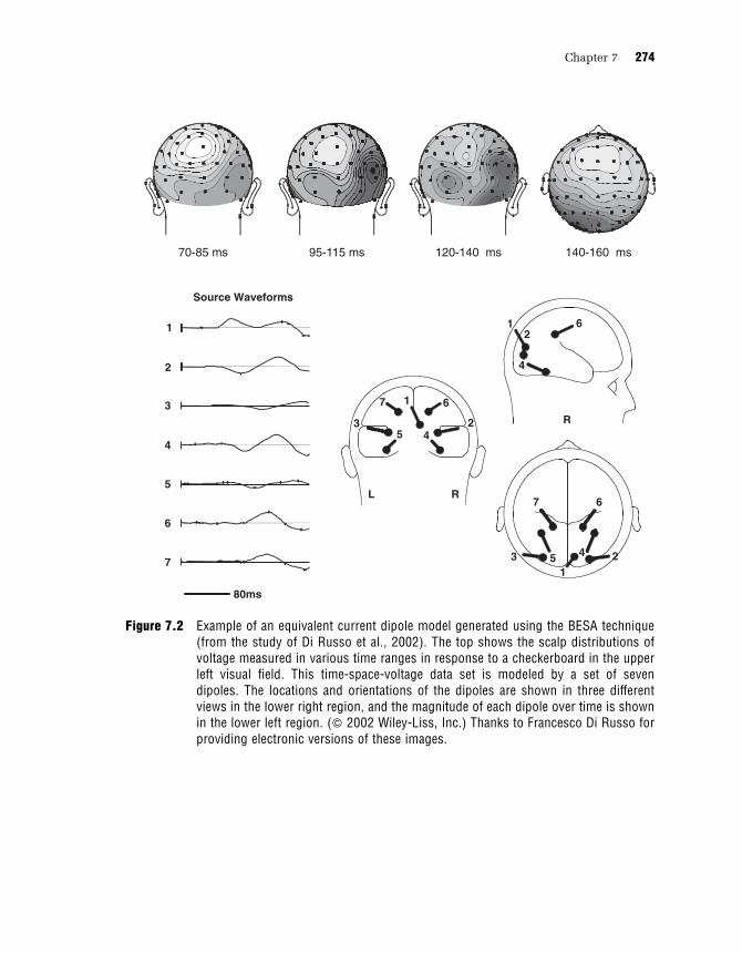
95-115 ms70-85 ms 140-160 ms120-140 ms
Source Waveforms
1
2
3
4
5
6
7
80ms
R
L R
12
4
6
1
2345
7 6
7 6
23 451
Figure 7.2 Example of an equivalent current dipole model generated using the BESA technique(from the study of Di Russo et al., 2002). The top shows the scalp distributions ofvoltage measured in various time ranges in response to a checkerboard in the upperleft visual field. This time-space-voltage data set is modeled by a set of sevendipoles. The locations and orientations of the dipoles are shown in three differentviews in the lower right region, and the magnitude of each dipole over time is shownin the lower left region. (> 2002 Wiley-Liss, Inc.) Thanks to Francesco Di Russo forproviding electronic versions of these images.
Chapter 7 274

substantial impact on the solution the algorithm ultimately
reaches. In fact, the most problematic aspect of the BESA tech-
nique is the fact that the user has a lot of control over the results
(this is called operator dependence); consequently the results may
be biased by the user’s expectations.
You can use several different strategies to select the number
of dipoles. One approach is to use principal components analysis
(PCA) to determine how many underlying spatial distributions of
activity contribute to the observed distribution of voltage over the
scalp. This technique can work well in some cases. However, if
the magnitudes of two dipoles are correlated with each other over
time, they may be lumped together into a single component. Thus,
the number of components identified by PCA can only provide a
lower bound on the number of dipoles.
Another strategy is to start by using one or two dipoles to create
a model of the early part of the waveform, under the assumption
that the response begins in one or two sensory areas. Once a stable
solution is reached for the early part of the waveform, the time
window is increased and new dipoles are added while the original
dipoles are held constant. This procedure is then repeated with a
larger and larger time window. This procedure makes some sense,
but it has some shortcomings. First, at least a dozen visual areas
are activated within 60 ms of the onset of activity in visual cortex
(Schmolesky et al., 1998), so representing the early portion of the
waveform with one or two dipoles is clearly an oversimplification.
Second, some error is likely in any dipole solution, and small
errors in the initial dipoles will lead to larger errors in the next set
of dipoles, and the location estimates will become increasingly in-
accurate as you add more and more dipoles.
A third strategy is to use preexisting knowledge about the brain
to determine the number of dipoles. For example, if you use differ-
ence waves to isolate the lateralized readiness potential, it would
be reasonable to start with the assumption that two dipoles are
present, one in each hemisphere.
ERP Localization 275

There are also several strategies that you can use for determining
the starting positions and orientations of the dipoles, and different
strategies will lead to different results. Unfortunately, most papers
using the BESA technique describe the model produced by one or
two different starting positions. Almost every time I have read a
paper that used the BESA technique, I wished the authors had
provided a detailed description of the results that would have
been obtained with a wide variety of different starting locations. It
would be possible for researchers to do this. Indeed, Aine, Huang,
and their colleagues have developed what they call a multi-start
approach to localization, in which they apply the localization algo-
rithm hundreds or even thousands of times with different starting
parameters (Aine et al., 2000; Huang et al., 1998). It is then possi-
ble to determine which dipole locations occur frequently in the
solutions and are therefore relatively independent of the starting
parameters.
Another strategy is to start with dipoles in locations that are
based on preexisting knowledge about the brain. The locations
could be based on general knowledge (e.g., the location of primary
and secondary auditory areas), or they could be based on specific
results from previous experiments (e.g., activation centers from
a similar fMRI experiment). When using the latter approach, re-
searchers sometimes say that the solution is based on seeded
dipoles, and some studies have explicitly shown that similar
results were obtained with random dipole locations and seeded
dipoles (e.g., Heinze et al., 1994). This is, in some ways, a reason-
able approach. However, it seems likely to lead to a confirmation
bias, increasing the likelihood that the expected results will be
obtained even if they are not correct.
Shortcomings of the BESA Approach
The BESA approach has several shortcomings, but the most signif-
icant problem is that there is no mathematically principled means
Chapter 7 276

of quantifying the accuracy of a solution. Specifically, in the pres-
ence of noise, it is possible for a substantially incorrect solution to
have the same (or lower) residual variance than the correct solu-
tion. Even with minimal noise, it is possible for a substantially in-
correct solution to have a very low residual variance (especially
when using more than a few dipoles). One reason for this is that
each BESA dipole has five free parameters (plus a time-varying
magnitude parameter). Thus, a model with only six dipoles has
thirty free parameters, and a relatively large error in one of these
parameters can easily be offset by small adjustments in the other
parameters, resulting in low residual variance. Even if only one
dipole is present, the BESA solution may be inaccurate due to
noise in the data and errors in the head model. Without some
means of quantifying the likelihood that a solution is correct or
even nearly correct, it’s hard to use a BESA solution to provide
strong support for or against a hypothesis.
The second most significant shortcoming of the BESA technique
is the operator dependence of the technique (as mentioned briefly
in the previous section). In addition to setting the number and ini-
tial positions of the dipoles, a researcher can adjust several other
parameters that control how the algorithm adjusts the positions
and orientations of the dipole while searching for the configuration
with the least residual variance. Moreover, at several points in the
process, the researcher makes subjective decisions about adding or
deleting dipoles from the solution or changing various constraints
on the dipoles. I have seen ERP researchers spend weeks applying
the BESA technique to a set of data, playing around with different
parameter settings until the solution ‘‘looks right.’’ Of course, what
‘‘looks right’’ is often a solution that will confirm the researcher’s
hypothesis (or at least avoid disconfirming it).
Another significant shortcoming of the BESA technique is that
it will produce an incorrect solution if the number of dipoles is
incorrect. It is difficult or impossible to know the number of
dipoles in advance, especially in an experiment of some cognitive
ERP Localization 277

complexity, so this is a significant limitation. Moreover, BESA uses
a discrete dipole to represent activity that may be distributed
across a fairly large region of cortex, and this simplification may
lead to substantial errors.
A Simulation Study
There have been a variety of tests of the accuracy of equivalent cur-
rent dipole localizations, but they have mostly used only one or
two simultaneously active dipoles (see, e.g., Cohen & Cuffin, 1991;
Leahy et al., 1998). These simulations are useful for assessing the
errors that might be likely in very simple sensory experiments, but
they do not provide meaningful information about the errors that
might occur in most cognitive neuroscience experiments.
Miltner et al. (1994) performed the most informative simulation
study in the context of cognitive neuroscience. This study used
BESA’s spherical, three-shell head model to simulate a set of
dipoles and produce corresponding ERP waveforms from thirty-
two electrode sites. From these ERP waveforms, nine participants
attempted to localize the dipoles using BESA. The participants
consisted of ERP researchers with various levels of expertise with
BESA (including three with very high levels of expertise).1 The
participants were told that the data were simulated responses from
left somatosensory stimuli that were presented as the targets in an
oddball task, and they were given the task of trying to localize the
sources. The simulation comprised ten dipoles, each of which was
active over some portion of a 900-ms interval. White noise was
added to the data to simulate the various sources of noise in real
ERP experiments. The simulation included two dipoles in left pri-
mary somatosensory cortex (corresponding to the P100 wave and
an early portion of the N150 wave), a mirror-symmetrical pair of
dipoles in left and right secondary somatosensory cortex, midline
dipoles in prefrontal and central regions, and mirror-symmetrical
pairs of dipoles in medial temporal and dorsolateral prefrontal
regions.
Chapter 7 278

This is a fairly large set of dipoles,2 but the participants’ task
was made easier by at least seven factors: (1) the solution included
several dipoles that were located exactly where they would be
expected (e.g., the primary and secondary somatosensory areas);
(2) three of the dipole pairs were exactly mirror-symmetrical
(which matches a typical BESA strategy of assuming mirror
symmetry at the early stages of the localization process); (3) the
spherical BESA head model was used to create the simulations,
eliminating errors due to an incorrect forward solution; (4) the tem-
poral overlap between the different dipoles was modest (for most
of the dipoles, there was a time range in which only it and one
other dipole or mirror-symmetrical dipole pair were strongly
active); (5) with the exception of the two dipoles in primary soma-
tosensory cortex, the dipoles were located fairly far away from
each other; (6) the white noise that was added was more easily fil-
tered out than typical EEG noise and was apparently uncorrelated
across sites; and (7) the simulation used discrete dipoles rather
than distributed regions of activation.
Despite the fact that the simulation perfectly matched the as-
sumptions of the BESA technique and was highly simplified, none
of the participants reached a solution that included all ten dipoles
in approximately correct positions. The number of dipoles in the
solutions ranged from six to twelve, which means that there were
several cases of missing dipoles and/or spurious dipoles. Only
two of the nine participants were able to distinguish between the
midline prefrontal and midline central dipoles, and the other
seven participants tended to merge them into a single dipole even
though the actual dipoles were approximately 5 cm apart.
Across all dipoles that appeared to be localized by the partici-
pants, the average localization error was approximately 1.4 cm,
which doesn’t sound that bad. However, this was a simplified sim-
ulation based on the BESA head model, and the errors with real
data are likely to be greater. Moreover, there were many cases in
which an individual dipole’s estimated location was 2–5 cm from
the actual dipole’s location, and the mean errors across dipoles for
ERP Localization 279

individual participants were as high as 2 cm. To be fair, however,
I should note that most of the participants provided a reasonably
accurate localization of one of the two primary somatosensory
dipoles, the secondary somatosensory dipoles, the medial temporal
lobe dipoles, and the dorsolateral prefrontal dipoles. But each of
the nine participants had at least one missing dipole, one spurious
dipole, or one mislocalization of more that 2 cm.
From this study, we can draw two main conclusions. First, in
this highly simplified situation, dipoles were often localized with
a reasonable degree of accuracy, with an average error of 1–2 cm
for most of the participants (relative to a 17-cm head diameter).
Thus, when reality does not deviate too far from this simplified sit-
uation, the BESA technique can potentially provide a reasonable
estimate of the locations of most of the dipoles most of the time.
However, some of the simplifications seem quite far from reality,
so it is entirely possible that average errors will be considerably
larger with most real data sets.
The second main conclusion is that any single dipole in a given
multiple-dipole BESA model has a significant chance of being sub-
stantially incorrect, even under optimal conditions. Dipoles may
be mislocalized by several centimeters or completely missed; mul-
tiple dipoles may be merged together, even if they are fairly far
apart; and spurious dipoles may be present in the model that corre-
spond to no real brain activity. Thus, even if the average error is
only 1–2 cm for most dipoles, this simulation suggests that BESA
solutions for moderately complex data sets may typically contain
at least one missing dipole, one spurious dipole, or one 2–5 cm lo-
calization error. And the accuracy of the technique is presumably
even worse for real data sets that deviate from the simplifications
of this simulation.
Although the BESA technique has been widely used over the
past twenty years, most ERP researchers now appreciate its limita-
tions. There is a clear trend away from this technique and toward
more sophisticated equivalent current dipole approaches and dis-
tributed source approaches.
Chapter 7 280

Distributed Source Approaches
General Approach
Instead of using a small number of equivalent current dipoles to
represent the pattern of neural activity, it is possible to divide the
brain up into a small number of voxels and find a pattern of activa-
tion values that will produce the observed pattern of voltage on the
surface of the scalp. For example, you could divide the surface of
the brain into a hundred little cubes. Each cube would contain
three dipoles, one pointing upward, one pointing forward, and
one pointing laterally (a single dipole of an arbitrary orientation
can be simulated by varying the relative strengths of these three
dipoles). You could then find a pattern of dipole strengths that
would yield the observed distribution of voltage on the surface of
the head. This would provide you with an estimate of the distribu-
tion of electrical activity throughout the brain.
The problem with this approach is that even this relatively
coarse parcellation of the brain requires that you compute 300
different dipole strengths. That is, your model has 300 free param-
eters to be estimated. Generally speaking, you need at least as
many independent data points as you have free parameters, and
even if you have voltage measurements from 300 electrodes,
they are contaminated by noise and are not independent of each
other. Consequently, there are many different sets of strengths of
the 300 dipoles that could produce the observed ERP scalp distri-
bution. This is the problem of nonuniqueness. And it would
get even worse if we wanted to divide the brain into even smaller
voxels.
Cortically Constrained Models
Researchers have developed several strategies to avoid the non-
uniqueness problem. One strategy is to reduce the number of
dipoles by assuming that scalp ERPs are generated entirely by
ERP Localization 281

currents generated in the cerebral cortex, flowing perpendicular to
the cortical surface (which is a reasonable assumption in most
cases). Instead of using a set of voxels that fills the entire volume
of the brain, with three dipoles per voxel, this approach uses struc-
tural MRI scans to divide the cortical surface into hundreds or
thousands of small triangles, each with a single dipole oriented
perpendicular to the cortical surface. This cortically constrained
approach dramatically reduces the number of free parameters in
the model (although some error may be introduced by inaccuracies
in the cortical surface reconstruction). The result is a model of the
distribution of electrical activity over the cortical surface.
Figure 7.3 illustrates this approach, with a slice through a car-
toon brain that shows the cortical surface and recording electrodes
for the left hemisphere. The cortical surface has been divided into
a number of small patches, and each patch is treated as a dipolar
current source pointing perpendicular to the cortical surface. This
reduces the number of dipole locations and orientations compared
to dividing the entire volume of the brain into voxels, each of
which contains three dipoles. However, the number of dipoles
needed in a real experiment is still very large (usually in the hun-
dreds or thousands), and there is still no unique pattern of dipole
strengths that can account for the observed distribution of voltage
on the scalp. That is, the use of a cortically constrained model
reduces the number of internal patterns of activity that could ex-
plain the observed distribution of voltage over the scalp, but it
does not bring the number all the way to one (i.e., to a unique
solution).
The non-uniqueness problem in cortically constrained models
can be appreciated by considering sources 15 and 16 in figure 7.3.
These sources are almost perfectly parallel to each other, but they
are inverted in orientation with respect to each other (i.e., the outer
surface of the cortex points downward for source 15 and upward
for source 16). This is a common occurrence given the extensive
foldings of the human cerebral cortex. The non-uniqueness prob-
lem occurs because any increase in the magnitude of source 15
Chapter 7 282

can be cancelled by an increase in the magnitude of source 16,
with no change in the distribution of voltage on the surface.
The Minimum Norm Solution
To get around the nonuniqueness problem (for both whole-brain
and cortically constrained models), Hamalainen and Ilmoniemi
(1984) proposed adding an additional constraint to the system. This
constraint is based on the fact that the cancellation problem—as
S0
S5
E0
E5
E1
E6
E2
E3
E4
S10
Cortex
Skull andScalp
Sources
S15
S16
S20
S25
S29
Figure 7.3 Example of the electrical sources and measurement electrodes used by corticallyconstrained distributed source localization methods. The figure shows a coronalsection through the brain. The cortex is divided into a large number of patches thatare assumed to be the electrical sources (labeled S0–S29 here). Each source ismodeled as a dipole that is centered in the corresponding cortical patch and ori-ented perpendicular to the patch. The voltage corresponding to each source propa-gates through the brain, skull, and scalp to reach the recording electrodes (labeledE0–E6), and the voltages from the different sources simply sum together.
ERP Localization 283
exemplified by sources 15 and 16 in figure 7.3—allows the magni-
tudes of nearby sources to become huge without distorting the dis-
tribution of voltage on the scalp. These huge magnitudes are a
biologically unrealistic consequence of the modeling procedure,
and it therefore makes sense to eliminate solutions that have huge
magnitudes. Thus, Hamalainen and Ilmoniemi (1984) proposed
selecting the one solution that both produces the observed scalp
distribution and has the minimum overall source magnitudes.
This is called the minimum norm solution to the problem of find-
ing a unique distribution of source magnitudes.
One shortcoming of the minimum norm solution is that it is
biased toward sources that are near the surface, because a larger
magnitude is necessary for a deep source to contribute as much
voltage at the scalp as a superficial source. However, this problem
can be solved by using a depth-weighted minimum norm solu-
tion that weights the magnitudes of each source according to its
depth when finding the solution with the minimum overall source
magnitudes.
Other researchers have proposed other types of minimum norm
solutions that reflect different constraints. The most widely used
of these alternatives is the low-resolution electromagnetic tomo-
graphy (LORETA) technique, which assumes that the voltage will
change gradually (across the volume of the brain or across the cor-
tical surface) and selects the distribution of source magnitudes that
is maximally smooth (Pascual-Marqui, 2002; Pascual-Marqui et al.,
2002; Pascual-Marqui, Michel, & Lehmann, 1994). The smoothness
constraint may be reasonable in many cases, but sharp borders
exist between adjacent neuroanatomical areas, and these borders
would sometimes be expected to lead to sudden changes in cortical
current flow. Indeed, if an experimental manipulation is designed
to activate one area (e.g., V3) and not an adjacent area (e.g., V4),
then the goals of the experiment would be incompatible with an
assumption of smoothness. On the other hand, gradual changes in
activity are probably the norm within a neuroanatomical area, so
the smoothness constraint may be appropriate in many cases. Note
Chapter 7 284

also that, because of its smoothness constraint, the LORETA tech-
nique is appropriate only for finding the center of an area of acti-
vation and not for assessing the extent of the activated area. In
contrast, nothing about the original and depth-weighted minimum
norm solutions will prevent sharp borders from being imaged.
It is possible to combine empirical constraints with these mathe-
matical constraints. For example, Dale and Sereno (1993) describe
a framework for using data from functional neuroimaging to pro-
vide an additional source of constraints that can be combined with
the minimum norm solution (see also George et al., 1995; Phillips,
Rugg, & Friston, 2002; Schmidt, George, & Wood, 1999). Like the
LORETA approach, this approach has the advantage of using bio-
logical information to constrain which solution is chosen. How-
ever, it is easy to conceive of situations in which an fMRI effect
would not be accompanied by an ERP effect or vice versa (see
Luck, 1999), so the addition of this sort of neuroimaging-based
constraint may lead to a worse solution rather than a better one. It
may also produce a confirmation bias: when you use fMRI data to
constrain your ERP localization solution, you’re increasing the
likelihood of finding a match between the ERP data and the fMRI
data even if the ERP is not generated at the locus of the fMRI
BOLD signal. A simulation study suggested that the most problem-
atic situation arises when an ERP source is present without a corre-
sponding fMRI source (Liu, Belliveau, & Dale, 1998). This study
also indicated that the resulting distortions are reasonably small if
the source localization algorithm assumes a less-than-perfect corre-
spondence between the ERP and fMRI data. It remains to be seen
whether the use of fMRI data to probabilistically constrain ERP
source localization leads to substantial errors when applied to real
data.
Unlike equivalent source dipole approaches, minimum norm-
based techniques will always find a unique solution to the inverse
problem, and they do it largely automatically. However, a unique
and automatic solution is not necessarily the correct solution. The
correctness of the solution will depend on the correctness of the
ERP Localization 285

assumptions. As Ilmoniemi (1995) discussed, an approach of this
type will provide an optimal solution if its assumptions are valid,
but different sets of assumptions may be valid for different data
sets. For example, if one applies the LORETA technique to the
three-dimensional volume of the brain without first creating a
model of the cortical surface, the smoothness assumption will al-
most certainly be violated when areas that are distant from each
other along the cortical surface abut each other due to the folding
pattern of the cortex. But if the smoothness constraint is applied
along the reconstructed 2-D cortical surface, then this assumes
that subcortical regions do not contribute to the data, which may
be incorrect.
The Added Value of Magnetic Recordings
As described in chapter 1, the EEG is accompanied by a magnetic
signal, the MEG, and event-related electrical potentials (ERPs) are
accompanied by event-related magnetic fields (ERMFs). Because
the skull is transparent to magnetism, it does not blur the MEG sig-
nal, and this leads to improved spatial resolution for MEG record-
ings. Another benefit of MEG is that, because magnetism passes
unimpeded through the head, MEG/ERMF localization does not re-
quire a model of the conductances of the head; it simply requires a
model of the overall shape of the brain. Thus, it can be advanta-
geous to apply localization techniques to ERMFs rather than ERPs.
ERMF localization faces the same non-uniqueness problem as
ERP localization, but combining ERP and ERMF data provides a
new set of constraints that can aid the localization process. The
main reason for this is that the voltage field and the magnetic field
run in different directions, and they therefore provide complemen-
tary information. As figure 7.4A illustrates, the magnetic field runs
in circles around the current dipole. When the current dipole is
oriented in parallel to the skull, the magnetic field exits the skull
on one side of the dipole and reenters the skull on the other side
(figure 7.4B). The strength of the magnetic field varies as a function
Chapter 7 286

A
CurrentDipole
Electrical Potential Magnetic Field
MagneticField
B C
D
Skull
Magnetic FieldLeaving Head
Magnetic FieldEntering Head
Figure 7.4 Relationship between an electrical dipole and its associated magnetic field. An elec-trical dipole has a magnetic field running around it (A), and when the dipole isroughly parallel to the surface of the head, the magnetic field leaves and reentersthe head (B). If the dipole is oriented radially with respect to the head, the magneticfield does not vary across the surface of the head (C). When a dipole runs parallel tothe surface of the head (represented by the arrow in D), there is a broad region ofpositive voltage at the positive end (solid lines) and a broad region of negativevoltage at the negative end (dashed lines), separated by a line of zero voltage (rep-resented by the dotted line). The magnetic field, in contrast, consists of magneticflux leaving the head on one side of the dipole (solid lines) and reentering the headon the other side (dashed lines), separated by a line of no net flux (dotted line).Thanks to Max Hopf for providing the electrical and magnetic distributions shownin (D).
ERP Localization 287

of distance from the dipole, just like the strength of the electrical
field, but the voltage distribution is broader due to the blurring of
the scalp (figure 7.4D). In addition, the magnetic and electrical dis-
tributions are oriented at 90 degrees with respect to each other. As
figure 7.4D shows, the positive and negative electrical potentials
appear at the positive and negative ends of the dipole, and the line
of zero voltage runs perpendicularly through the center of the
dipole. The efflux and influx of the magnetic field, in contrast, oc-
cur on the left and right sides of the dipole, and the zero flux line
runs in parallel with the orientation of the dipole.
MEG fields differ from EEG fields in another key way as well. If
the current dipole is perfectly perpendicular to the skull, as in
figure 7.4C, the magnetic field does not exit and reenter the head,
and it is essentially invisible. As the dipole tilts from perpendicu-
lar toward parallel, a recordable magnetic field begins to appear
again. In contrast, a large and focused voltage will be present di-
rectly over a perpendicular dipole. A dipole near the center of the
head will act much like a perpendicular dipole, generating a rea-
sonably large voltage on the surface of the scalp that is accompa-
nied by a magnetic field that does not exit and reenter the head
and is therefore effectively invisible. Thus, magnetic signals are
largest for superficial dipoles that run parallel to the surface of the
skull, and fall off rapidly as the dipoles become deeper and/or per-
pendicularly oriented, but voltages do not fall off rapidly in this
manner.
The different effects of dipole depth and orientation on electrical
and magnetic signals provide an additional set of constraints on
source localization solutions. In essence, there are many internal
source configurations that can explain a given electrical distribu-
tion, and there are also many internal source configurations that
can explain a given magnetic distribution. But there will be far
fewer configurations than can explain both the electrical distribu-
tion and the magnetic distribution. Consequently, the combination
of magnetic and electrical data is substantially superior to either
type of data alone. The main drawbacks of combining magnetic
Chapter 7 288

and electrical data compared to using magnetic data alone are that
(a) a more complex head model is needed for the electrical data,
and (b) some effort is required to ensure that the electrical and
magnetic data are in exactly the same spatial reference frame.
Can We Really Localize ERPs?
Each of the source localization techniques described in this chap-
ter has shortcomings. Of course, any scientific technique has
limitations and shortcomings, but the shortcomings of source local-
ization techniques are fundamentally different from the shortcom-
ings of other techniques for localization of function. This section
will explore these differences and consider a new approach that
seems more promising.
Source Localization as Model Fitting
To understand the essence of ERP source localization, it is useful
to compare it with a ‘‘true’’ neuroimaging technique, such as PET.
In the most common PET approach, radioactively labeled water
molecules travel through the bloodstream, where their diffusion
properties are straightforward. Consequently, the number of radio-
active molecules in a given volume of the brain can be directly re-
lated to the flow of blood through that part of the brain. When a
labeled water molecule decays, it gives off a positron, which trav-
els a known distance (or distribution of distances) before colliding
with an electron. This collision leads to a pair of annihilation pho-
tons that travel in opposite directions along the same line. When
these high-intensity photons are picked up simultaneously by two
detectors within the ring of detectors around the subject, there is a
high likelihood that they were generated somewhere along the line
between the two detectors, and the decaying isotope is known to
have been within a certain distance from this line. Thus, by com-
bining the known physics of radiation with various probability
distributions, one can directly compute the maximum likelihood
ERP Localization 289
location of the radioactively labeled water molecules and the mar-
gin of error of this location. The story is analogous, although more
complicated, for fMRI.
Because the ERP localization problem is underdetermined, main-
stream ERP localization techniques employ a different approach.
That is, they do not simply compute the maximum likelihood loca-
tion of an ERP source, along with a margin of error, on the basis of
the physics of electricity and magnetism. Instead, ERP localization
techniques generate models of the underlying distribution of elec-
trical activity, and these models are evaluated in terms of their
ability to satisfy various constraints. The most fundamental con-
straint, of course, is that a given model must recreate the observed
distribution of voltage over the surface of the head. However, a cor-
rect model may not fit the data exactly, because noise in the data
distorts the observed distribution. Consequently, any internal con-
figuration that is, say, 95 percent consistent with the observed
scalp distribution might be considered acceptable. Unfortunately,
there will be infinitely many internal configurations that can ex-
plain an observed scalp distribution, especially when only a 95
percent fit is required.
Additional constraints are then added to select one internal con-
figuration from the many that can explain the observed scalp distri-
bution. Each source localization technique embodies a different set
of these additional constraints, and the constraints can be either
mathematical (as in the use of the minimum norm) or empirical
(as in the use of fMRI data to constrain ERP localizations). The
most straightforward empirical constraint is the use of structural
MRI scans to constrain the source locations to the cortical surface.
However, this alone does not lead to a unique solution (and it may
not always be the case that all scalp ERP activity arises from the
cortex). Researchers therefore add other constraints, but there is
usually no way of assessing whether these constraints are correct
and sufficient.
The bottom line is that ERP localization leads to a model of the
internal configuration of electrical activity, not a measurement
Chapter 7 290

of the internal distribution of electrical activity. In contrast, PET
and fMRI provide measurements and not merely models. PET, for
example, provides a measurement of the internal distribution of
radioactively labeled blood. This measurement is derived from
more basic measurements, but that is true of most sophisticated
scientific measurements. And although the PET measurements are
not error-free, this is true of any measurement, and one can specify
the margin of error. It is more difficult to describe exactly what the
BOLD signal reflects in fMRI, but the location of this signal is mea-
sured with a known margin of error. In contrast, one cannot use
surface electrodes to measure the distribution of internal electrical
activity with a known margin of error.
People occasionally ask me how accurately ERPs can be local-
ized, hoping for a quantification of accuracy that they can compare
with the accuracy of PET and fMRI. My response is that the accu-
racy of ERP localization is simply undefined. That is, in the ab-
sence of any constraints beyond the observed scalp distribution,
radically different distributions of internal electrical activity would
produce the observed scalp distribution, and the margin of error is
essentially the diameter of the head.
Once constraints are added, some source localization approaches
could, in principle, quantify the margin of error. For example, it
would be possible to state that the estimated center of a region of
activation is within X millimeters of the actual center of the acti-
vated region. Or it would be possible to state that the amount of
estimated current flow within each patch of cortex is within Y per-
cent of the actual current flow. I’ve never seen anyone do this in
the context of a serious experiment, but it would be an extremely
useful addition to the source localization techniques. However,
the margin of error that could be specified in this manner would
be meaningful only if the constraints of the model were fully ade-
quate and the only sources of error arose from noise in the ERP
data (and perhaps errors in specifying the head model). If the con-
straints were insufficient, or if they reflected incorrect assump-
tions about the underlying neural activity, then the margin of error
ERP Localization 291

would be meaningless. Thus, the source localization techniques
that are currently in widespread use do not, in practice, provide a
meaningful estimate of the margin of error.
Probabilistic Approaches
The commonly used source localization techniques attempt to find
a single pattern of internal electrical activity that best explains the
observed scalp distribution (along with satisfying other implicit or
explicit constraints). When I read a paper that reports source local-
ization models, I always wonder what other distributions would fit
the data as well as, or almost as well as, the reported solution. Are
all reasonable solutions similar to the reported solution? Or are
there other solutions that are quite different from the reported solu-
tion but fit the data and the constraints almost as well? After all,
the presence of noise in the data implies that the correct solution
will not actually fit the data perfectly, so a solution that explains
only 97 percent of the variance may be closer to the correct solu-
tion than a solution that accounts for 100 percent of the variance.
Figure 7.5 shows a simulation presented by Koles (1998) that
illustrates this problem. Koles created a distributed source by using
several nearby dipoles arranged along a curved surface, and fit an
equivalent current dipole to the scalp distribution produced by
this distributed source. He placed model dipoles systematically at
a variety of locations, and measured the residual error for each of
these locations. As the right side of figure 7.5 shows, the error was
lowest near the location of the best equivalent current dipole, but
there wasn’t much difference in error over a fairly wide range of
locations. This is exactly the sort of information that one needs to
know when trying to evaluate a source localization model.
In my view, it is misguided to attempt to find a unique solu-
tion given the uncertainties inherent in ERP localization. A better
approach would be to report the entire range of solutions that fit
the data and constraints to some criterion level (e.g., a fit of 95 per-
cent or better). Moreover, it would be useful to report the range of
Chapter 7 292

solutions obtained as one adds and removes various constraints. If,
for example, one were to find high levels of estimated activity in
a particular region in almost any solution, no matter what con-
straints were used, then this would give us considerable confi-
dence that this region really contributed to the observed ERPs.
A few investigators have explored this general sort of approach.
For example, as described in the section on equivalent source
dipole approaches, Huang, Aine, and their colleagues (1998) have
developed a multi-start approach in which the dipole localization
procedure is run hundreds or thousands of times with different
starting positions. This makes it possible to see which dipole loca-
tions are found frequently, independent of the starting positions or
even the number of dipoles in the model. This approach poten-
tially solves the most significant shortcomings of equivalent source
dipole approaches. In particular, the solutions are largely operator-
independent, and it is possible to assess the likelihood that a given
A B
Skull
x
z
EquivalentSource
-1
0
1
-1
0
10
1
2
-log (J )
xz
Figure 7.5 Example of a distributed electrical source (A) and the amount of error that wouldoccur in estimating this source by a single dipole over a range of positions (B). Al-though a single point of minimum error exists, the amount of error varies little overa fairly wide range. (Adapted from Koles, 1998. > 1998 Elsevier Science IrelandLtd.) Thanks to Zoltan Koles for providing electronic versions of these images.
ERP Localization 293
dipole location occurred because of the starting positions of the
dipoles or because of incorrect assumptions about the number of
dipoles.
Although the multi-start approach addresses these shortcomings,
it still falls short of providing a quantitative description of the
probability that a particular brain area contributed to the observed
ERP data. That is, a dipole may have been found in a given region
in some percentage of the solutions, but the localization approach
does not guarantee that the space of adequate solutions is sampled
completely and evenly. However, Schmidt, George, and Wood
(1999) have developed a distributed source localization technique
based on Bayesian inference that provides a more sophisticated
means of assessing probabilities. This technique is similar to the
multi-start technique insofar as it generates thousands of potential
solutions. However, its basis in Bayes’s theorem allows it to pro-
vide a more complete and quantitative description of the space of
possible solutions. This is the most promising localization tech-
nique that I have seen. Unfortunately, it has not yet been widely
applied to real experiments, and other groups of researchers
have not yet thoroughly explored its limitations. Nonetheless, the
more general principle embodied by this approach and the multi-
start approach—which systematically explore the space of likely
solutions—seems like the best direction for the development of
source localization techniques.
Recommendations
I will end this chapter by providing some recommendations about
whether, when, and how you should use source localization tech-
niques. My basic conclusion is that ERP localization is extremely
difficult, and it should be attempted only by experts and only
when the solution space can be reduced by well-justified con-
straints, such as structural MRI data and the combination of elec-
trical and magnetic data. In addition, the most commonly used
techniques are useful primarily for obtaining converging evidence
rather than providing a conclusive, stand-alone test of a hypothe-
Chapter 7 294

sis, although ongoing developments may someday allow source lo-
calization data to provide definitive results.
Source Localization and Scientific Inference
To assess the value of source localization techniques, it is useful
to put them into the context of general principles of scientific infer-
ence. Perhaps the most commonly cited principle of scientific in-
ference is Popper’s (1959) idea of falsification. A commonly used,
although less commonly cited, extension of this idea is Platt’s
(1964) notion of strong inference, in which the best experiments
are those that differentiate between competing hypotheses, sup-
porting one and falsifying the other.
How do source localization techniques fare when judged by
these standards? Not well. I don’t think anyone really believes that
a single source localization model can conclusively falsify a hy-
pothesis or definitively decide between two competing hypotheses.
There are simply too many uncertainties involved in source local-
ization. On the other hand, it is rare that a single experiment us-
ing any method is 100 percent conclusive, so this standard may be
unrealistic.
A more flexible approach is to apply Bayes’s Theorem to scien-
tific inference. In this context, we can summarize Bayes’s Theorem
by stating that a new result increases the probability that a hypoth-
esis is true to the extent that (a) there is a high probability of that
result being true if the hypothesis is true, and (b) there is a low
probability of that result being true if the hypothesis is false. In
other words, a finding that is consistent with a hypothesis does
not give us much more faith in the hypothesis if the finding is
likely even if the hypothesis is wrong.
In this context, a given source localization model will have value
to the extent that it not only supports a specific hypothesis but is
also unlikely to have been obtained if the hypothesis is false. It’s
the second part of this equation that is especially problematic for
source localization models, at least as researchers typically use
them. As discussed in the previous section, source localization
ERP Localization 295

models provide an estimate of the internal distribution of electrical
activity, but they do not typically quantify the probability that the
estimate is incorrect (which is related to the probability that the
finding would be obtained even if the hypothesis is false). How-
ever, this problem can be overcome, at least in principle. For
example, the probabilistic approaches described in the previous
section are designed to provide information about the range of
possible solutions, making it possible to assess the probability that
activity would appear in a given location in the models even if the
corresponding brain location were not truly active. Thus, although
most source localization methods are not well suited for this kind
of scientific inference, this does not appear to be an intrinsic limi-
tation of the entire source localization enterprise.
Another commonly cited principle of scientific inference is the
idea of converging evidence, which was first developed in the con-
text of perception research (Garner, Hake, & Eriksen, 1956) but is
now widely used in cognitive neuroscience. The basic idea is that
many interesting questions about the mind cannot be answered by
means of any single method, but a clear answer can be obtained
when many methods with different strengths and weaknesses con-
verge on the same conclusion. This is a common use of source
localization models. That is, the researchers understand that the
models are not conclusive evidence that the ERPs are generated in
specific brain regions, but they believe that the models are valuable
insofar as they converge with data from other sources. Box 7.1 pro-
vides an example of this from my own research.
Until source localization techniques routinely provide meaning-
ful, quantitative information about the probability that a given
model is correct, the main role of source localization models will
be to provide converging evidence. However, not all cases of con-
verging evidence are created equal: If a model uses weak methods
to create a given source localization model, then this model will
provide only weak converging evidence. And the value of such
models is questionable, especially given the time and expense
often involved in the modeling process. At present, source local-
Chapter 7 296
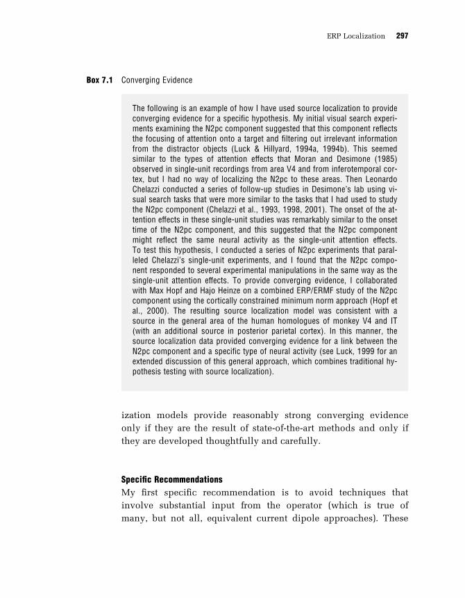
ization models provide reasonably strong converging evidence
only if they are the result of state-of-the-art methods and only if
they are developed thoughtfully and carefully.
Specific Recommendations
My first specific recommendation is to avoid techniques that
involve substantial input from the operator (which is true of
many, but not all, equivalent current dipole approaches). These
Box 7.1 Converging Evidence
The following is an example of how I have used source localization to provideconverging evidence for a specific hypothesis. My initial visual search experi-ments examining the N2pc component suggested that this component reflectsthe focusing of attention onto a target and filtering out irrelevant informationfrom the distractor objects (Luck & Hillyard, 1994a, 1994b). This seemedsimilar to the types of attention effects that Moran and Desimone (1985)observed in single-unit recordings from area V4 and from inferotemporal cor-tex, but I had no way of localizing the N2pc to these areas. Then LeonardoChelazzi conducted a series of follow-up studies in Desimone’s lab using vi-sual search tasks that were more similar to the tasks that I had used to studythe N2pc component (Chelazzi et al., 1993, 1998, 2001). The onset of the at-tention effects in these single-unit studies was remarkably similar to the onsettime of the N2pc component, and this suggested that the N2pc componentmight reflect the same neural activity as the single-unit attention effects.To test this hypothesis, I conducted a series of N2pc experiments that paral-leled Chelazzi’s single-unit experiments, and I found that the N2pc compo-nent responded to several experimental manipulations in the same way as thesingle-unit attention effects. To provide converging evidence, I collaboratedwith Max Hopf and Hajo Heinze on a combined ERP/ERMF study of the N2pccomponent using the cortically constrained minimum norm approach (Hopf etal., 2000). The resulting source localization model was consistent with asource in the general area of the human homologues of monkey V4 and IT(with an additional source in posterior parietal cortex). In this manner, thesource localization data provided converging evidence for a link between theN2pc component and a specific type of neural activity (see Luck, 1999 for anextended discussion of this general approach, which combines traditional hy-pothesis testing with source localization).
ERP Localization 297

techniques are so prone to experimenter bias that they can provide
only the weakest sort of converging evidence. In fact, I would argue
that these models are often worse than no models at all, because
they provide the illusion of strong evidence when in fact the evi-
dence is weak. The one exception to this recommendation is that
these approaches may be adequate when a combination of three
criteria are met: (1) the data are very clean; (2) you can be sure
that only one or perhaps two dipoles are present; and (3) you have
good reason to believe that the electrical activity is relatively fo-
cused rather than being distributed over a large region. Localiza-
tion is fairly easy under such conditions, and validation studies
have shown that localization errors average approximately 1 cm or
less when these criteria are met (see, e.g., Cuffin et al., 1991; Leahy
et al., 1998).
My second specific recommendation is to obtain structural MRI
scans from each subject so that you can create a reasonably ac-
curate head model and use one of the cortically constrained
approaches (which typically involve distributed source solutions
rather than equivalent current dipole solutions). For most experi-
ments in cognitive neuroscience, it is very likely that the activity
is generated exclusively in the cortex with a perpendicular orien-
tation, and this provides a powerful constraint that reduces the
solution space considerably. The most common versions are the
depth-weighted minimum norm and LORETA techniques, de-
scribed previously in this chapter. LORETA is well suited for
situations in which (a) you want to determine the center of each
activated region, (b) you do not care about the spatial extent of the
activated regions, and (c) the activated regions are well separated
from each other. If these conditions are met, LORETA appears to
work quite well (see, e.g., the impressive LORETA/fMRI corre-
spondence obtained by Vitacco et al., 2002). If these conditions
are not met, I would recommend using the depth-weighted mini-
mum norm approach.
My third recommendation is to use difference waves to isolate a
single component (or small set of components; see chapter 2 for
Chapter 7 298

more discussion). The more components are active, the more of
a mess you will have to sort out. Equivalent current dipole ap-
proaches become particularly problematic when more than a few
sources are present, but this can also be a problem for distributed
source approaches.
My fourth recommendation is to record ERMFs in addition to
ERPs. ERMFs have two major advantages over ERPs. First, they are
not blurred and distorted by the high resistance of the skull, lead-
ing to greater resolution and a smaller space of possible solutions
(see, e.g., the simulation results of Leahy et al., 1998). Second, be-
cause biological tissues are transparent to magnetism, it is not nec-
essary to create a model of the conductivities of the brain, skull,
and scalp, and this eliminates one possible source of error. ERMF
recordings do have a couple disadvantages, though. First, they are
very expensive, both in terms of the initial capital investment and
the maintenance costs (particularly the coolant). Second, ERMF
recordings will not be able to detect sources that are deep or per-
pendicular to the surface of the head (note, however, that this
becomes an advantage rather than a disadvantage when ERMFs
are combined with ERPs). In my experience, source localization is
just too uncertain when based on ERPs alone.
The bottom line is that source localization is extremely difficult,
and any serious attempt at localization will require sophisticated
methods and considerable costs (both in terms of time and money).
If you simply record ERPs from a large number of channels and
try to fit a half dozen dipoles to the data with no additional con-
straints, it’s not clear what you will have learned. At best, you will
gain some weak converging evidence. At worst, you will be misled
into believing in a solution that is simply incorrect.
I would like to end by noting that the clear strength of the ERP
technique is its temporal resolution, not its ability to localize brain
function. It is therefore sensible to use this technique primarily to
answer questions that require temporal resolution, leaving ques-
tions about localization of function to other techniques. When a
question requires a combination of temporal and spatial resolution,
ERP Localization 299

a combination of ERPs, ERMFs, structural MRI scans, and fMRI
data may provide reasonably strong evidence, but the commonly
used methods for localizing ERPs/ERMFs do not make it clear
how strong the evidence is. As new techniques are developed—
particularly those based on probabilistic approaches—we may
eventually get to the point where we can have a reasonably high
(and known) level of certainty.
Suggestions for Further Reading
The following is a list of journal articles and book chapters
that provide useful information about ERP and MEG source
localization.
Dale, A. M., & Sereno, M. I. (1993). Improved localization of corti-
cal activity by combining EEG and MEG with MRI cortical sur-
face reconstruction: A linear approach. Journal of Cognitive
Neuroscience, 5, 162–176.
George, J. S., Aine, C. J., Mosher, J. C., Schmidt, D. M., Ranken, D.
M., Schlitt, H. A., Wood, C. C., Lewine, J. D., Sanders, J. A.,
& Belliveau, J. W. (1995). Mapping function in the human
brain with magnetoencephalography, anatomical magnetic res-
onance imaging, and functional magnetic resonance imaging.
Journal of Clinical Neurophysiology, 12, 406–431.
Hamalainen, M. S., Hari, R., Ilmonieni, R. J., Knuutila, J., & Lounas-
maa, O. V. (1993). Magnetoencephalography—theory, instru-
mentation, and applications to noninvasive studies of the
working human brain. Review of Modern Physics, 65, 413–497.
Koles, Z. J. (1998). Trends in EEG source localization. Electroence-
phalography & Clinical Neurophysiology, 106, 127–137.
Luck, S. J. (1999). Direct and indirect integration of event-related
potentials, functional magnetic resonance images, and single-
unit recordings. Human Brain Mapping, 8, 15–120.
Mangun, G. R., Hopfinger, J. B., & Jha, A. P. (2000). Integrating elec-
trophysiology and neuroimaging in the study of human brain
Chapter 7 300

function. In P. Williamson, A. M. Siegel, D. W. Roberts, V. M.
Thandi & M. S. Gazzaniga (Eds.), Advances in Neurology (Vol.
84, pp. 33–50). Philadelphia: Lippincott, Williams, & Wilkins.
Miltner, W., Braun, C., Johnson, R., Jr., Simpson, G. V., & Ruchkin,
D. S. (1994). A test of brain electrical source analysis (BESA):
A simulation study. Electroencephalography & Clinical Neuro-
physiology, 91, 295–310.
Pascual-Marqui, R. D., Esslen, M., Kochi, K., & Lehmann, D. (2002).
Functional imaging with low-resolution brain electromagnetic
tomography (LORETA): a review. Methods & Findings in Ex-
perimental & Clinical Pharmacology, 24 Suppl C, 91–95.
Scherg, M., Vajsar, J., & Picton, T. (1989). A source analysis of the
human auditory evoked potentials. Journal of Cognitive Neuro-
science, 1, 336–355.
Schmidt, D. M., George, J. S., & Wood, C. C. (1999). Bayesian infer-
ence applied to the electromagnetic inverse problem. Human
Brain Mapping, 7, 195–212.
Snyder, A. (1991). Dipole source localization in the study of EP
generators: A critique. Electroencephalography & Clinical Neu-
rophysiology, 80, 321–325.
ERP Localization 301


8 Setting Up an ERP Lab
This chapter describes how to set up an ERP lab, including advice
on selecting equipment and software for stimulus presentation,
data collection, and data analysis. There are certainly many ways
to set up an ERP lab, and some factors will depend on the topic
area of your research. However, the suggestions in this chapter
will provide a good starting point for almost anyone who is setting
up an ERP lab for the first time. Also, many of the suggestions in
this chapter are based on my experience, but there are often other
good ways of achieving the same goals, and it is worth asking a
variety of ERP researchers how they set up their labs. If you al-
ready have access to an ERP lab, you may find some good ideas for
improving the lab in this chapter (see especially box 8.1 later in
this chapter).
The Data Acquisition System
Computers
Figure 8.1 shows a diagram of a generic ERP data acquisition sys-
tem. It is usually desirable to have at least two and possibly three
computers. One computer presents the stimuli, and a second com-
puter records the EEG. These functions are not ordinarily combined
into a single computer, because each requires precise timing, and it
is difficult to coordinate two real-time streams of events in a single
computer. It is also very useful to have a third computer that pro-
vides real-time information about the subject’s performance on the
task. The stimulus presentation computer sometimes provides this

Headbox
Intercom
Intercom
ImpedanceMeter
Calibrator
Amplifier
EEGEEG
AmplifiedEEG
ElectricallyShieldedChamber
EventCodes
EventCodes
ResponseBox
ElectrodeCap
DigitizationStimulusPresentation
BehaviorMonitoring
VideoSplitter
Figure 8.1 Major components of a typical ERP recording system.
Chapter 8 304

function, but in this case performance information is usually sum-
marized at the end of each trial block rather than being displayed
in real time (and a real-time display is definitely better).
The computers will need some means of communicating with
each other in real time so that event codes can be sent to the digiti-
zation computer whenever an event of some sort occurs (e.g., a
stimulus or a response). These event codes are used as the time
locking points for averaging, so the timing must be precise. A con-
sistent delay is not a big problem, because you can shift the
averages in time to compensate for the delay. A variable delay,
however, is usually difficult to compensate for, and it will have
the effect of smearing out the ERP waveforms in time, distorting
the onset and offset times of the components and experimental
effects (just like a low-pass filter).
The stimulus presentation computer’s video output is usually
directed into a video splitter that serves two functions. First, it
splits the video signal so that the experimenter can see what the
subject is seeing (this is essential so that the experimenter can
intelligently monitor the EEG display and detect problems, such
as blinks and eye movements that certain stimuli may trigger). Sec-
ond, it amplifies the video signal so that one can use a relatively
long cable to get the video signal into the recording chamber. It
is important to use a high-quality, shielded video cable from the
splitter into the chamber to minimize electrical noise inside the
chamber and to avoid degradation of the video signal. As discussed
in chapter 3, it’s a good idea to enclose the video monitor in a Far-
aday cage to avoid bringing a large noise signal into the recording
chamber. I provide more information about the video system later
in this chapter, in the section on stimulus presentation.
Seating
In experiments using visual stimuli, the subject is seated at a spe-
cific distance from the video monitor. Even with a Faraday cage,
Setting Up an ERP Lab 305

some electrical noise may be picked up from the monitor, so the
subject should not be too close to it. I would suggest a minimum
distance of 70 cm, and 1–2 m is even better if the chamber is large
enough.
It is very important for the subject to be seated in a comfortable
position. In the early days of ERP recordings, very few electrodes
were used and auditory stimuli were more common than visual
stimuli. A large, padded recliner was the most sensible chair for
such experiments. This kept the subject comfortable, and mini-
mized any need for subjects to use their neck muscles to support
their heads, which in turn minimized EMG noise (see chapter 4).
However, when electrodes are placed over the back of the head, a
recliner doesn’t work as well: the head puts pressure on the elec-
trodes, and any small head movement will cause the electrodes to
move on the scalp, producing a large and sudden voltage shift.
If your experiments will require recording from electrodes on the
back of the head, I would not recommend using a recliner. Instead,
I would recommend a high-quality office chair that provides good
lumbar support and has an easy mechanism for height adjustment.
It is also preferable to use a chair that is on glides rather than
casters so that subjects do not move the chair around inside the
chamber. The position of the chair on the floor should be marked
so that you can correctly reposition the chair if it gets moved. I
would also recommend against using any kind of chin rest or other
head stabilization. Although you might think that this would re-
duce strain on the neck muscles, my experience has been that
chin rests become uncomfortable after 15 minutes or so (and most
ERP experiments require at least an hour of recording time).
Behavioral Responses
Most cognitive ERP experiments use a small set of behavioral re-
sponse alternatives, and only two to four buttons are usually neces-
sary. The most convenient device for responses is usually a small,
Chapter 8 306

lightweight, hand-held device of some sort. My lab uses computer
video game controllers. It is easy to find game controllers that are
very comfortable and lightweight, and they usually offer at least
four response buttons (which is enough for most experiments).
Various custom response devices are also possible, but they are
not usually as easy to hold and use as a game controller. A com-
puter keyboard is not usually very good, because it is too big to
rest on the subject’s lap, and if it’s on the table in front of the sub-
jects, EMG noise is likely to occur as the subjects hold their arms
up to the keyboard. If a keyboard is necessary because of a large
number of response alternatives, the data around the time of the
response may be contaminated by EMG noise, and eye movement
artifacts may be seen if the subject needs to look at the keyboard
to find the right key to press. However, it may be possible to design
the experiment so that the data around the time of the response are
not important. Also, it may be possible to use a keyboard tray to
minimize the need to hold the hands upward and outward to reach
the keyboard.
Devices such as keyboards and game pads are not designed for
real-time electrophysiological recording, and a delay may occur
between the time of the buttonpress and the time that the computer
records the buttonpress. Response times are usually so variable
that this small error will not matter. However, it may be a signifi-
cant problem if you are doing response-locked averaging. In such
cases, you will probably need some sort of custom response device
with known and consistent temporal properties. One way to ensure
precise timing is to use a response device with an analog output
that can be recorded via the ADC along with the EEG.
Electrode-Amplifier-Computer Connections
The EEG is picked up by the electrodes and travels through cables
to the amplifier system. Before they are amplified, the signals are
miniscule, and any electrical noise that the cables pick up will be
Setting Up an ERP Lab 307

relatively large compared to the EEG. Consequently, the cables be-
tween the electrodes and the amplifier system should be kept as
short as is practical. It is now possible to purchase electrodes with
built-in pre-amplifiers, which will increase the size of the EEG sig-
nal relative to any noise picked up by the cables. This is a good
idea conceptually, but I have not tested these electrodes and I don’t
know how well they work in practice.
Many EEG amplifier systems have a headbox that provides a
flexible means of connecting the electrodes to the amplifier. Flexi-
bility is important. For example, you want to be able to select a
common reference electrode for most of the channels (e.g., a mas-
toid or earlobe reference) while allowing other channels to use
a different reference electrode (e.g., eye movements are usually
recorded as the voltage between electrodes on either side of the
eyes). Because the output of the headbox is not amplified, the cable
from the headbox to the amplifier should be relatively short. Opti-
mally this cable should be shielded, especially if the actual ampli-
fier is outside the recording chamber. If the amplifier is inside the
chamber, an unshielded ribbon cable will probably be sufficient (a
ribbon cable keeps the active, reference, and ground signals close
to each other so that they pick up the same noise signals, and this
allows the differential amplifier to subtract away the noise).
If the amplifier is connected to AC power, it is usually best to
place it outside the recording chamber to avoid inducing noise in
the electrodes. If it is battery powered, it can probably be placed
inside the chamber, which is good because only amplified signals
will leave the chamber, where electrical noise is much greater.
Once the signals have been amplified, they are usually much larger
than any induced electrical noise, so you may use longer cables to
connect the amplifier to the digitization computer. However, some
noise may still be picked up at this stage, and some shielding may
be necessary even after the signals have been amplified. In one of
the recording rooms in my lab, we found that shielded cables were
necessary to avoid picking up noise between the amplifier and the
digitization computer.
Chapter 8 308

Recording Chamber
One of the most expensive elements of an ERP lab is the electri-
cally isolated chamber. These chambers are usually designed as
sound-attenuating chambers for hearing testing, broadcasting, or
auditory research, but some manufacturers offer electrical shield-
ing options. I have chambers made by Industrial Acoustics Com-
pany and Acoustic Systems, and they work quite well. In the late
1990s, I paid approximately US $11,000 for a medium-sized cham-
ber (including installation costs).
Is an electrically isolated chamber really necessary? Not always.
If there are not many significant sources of electrical noise nearby,
you might be able to get away with using a low-pass filter with a
half-amplitude cutoff around 30 Hz to get rid of line-frequency
noise. If you are just starting to do ERP research and you are not
sure how many experiments you will be doing, this might be a
reasonable choice. However, if you plan to do ERP research for
several years, the cost of a chamber isn’t really that high, and it’s a
worthwhile investment. Remember that any significant decreases
in signal-to-noise ratio will be very costly in terms of the number
of trials (or subjects) needed to get reliable ERP waveforms (see
chapter 3).
Don’t assume that the chamber effectively eliminates all sources
of electrical noise. Chambers often include AC outlets, fans, and
lights that may cause substantial electrical noise. In fact, the first
chamber I ever used induced so much noise that I was able to get
cleaner recordings outside the chamber than inside. I eventually
found the circuit breaker for the chamber, and turning it off elimi-
nated the noise. You can use the device described in chapter 3 (see
figure 3.3B) to find sources of noise inside the chamber.
Accessories
A few accessories are important in an ERP lab. First, it is usually
necessary to have an impedance meter to test electrode impedan-
ces while attaching the electrodes. Some amplification systems
Setting Up an ERP Lab 309

have this function built into them, which is very useful for de-
termining if impedance problems are occurring once you’ve
started collecting data. Second, some sort of calibrator is neces-
sary for measuring the actual gain of the amplifiers. Many ampli-
fication systems have a built-in calibrator, but you can purchase
an external calibrator if your amplification system does not
have its own calibrator. If possible, the calibrator should be able
to produce square-wave pulses triggered by the stimulus presenta-
tion computer. This will help you to determine if there are any
time delays in your event codes, and it will also make it easy for
you to see exactly what kinds of distortion the amplifier’s filters
produce.
A third important accessory is an intercom system that will
allow you to communicate with the subject during the record-
ings. When purchasing an intercom system, keep in mind that
you don’t want a system that is AC powered, because this will
introduce electrical noise into the recording chamber. I’ve tried
several different types of systems, and my preferred intercom
system consists of a pair of microphones and powered speakers
(which you can purchase at many places, such as Radio Shack).
One microphone is attached to the ceiling of the recording cham-
ber and is connected to a powered speaker outside the chamber.
The other microphone is mounted near the experimenter and is
connected to a powered speaker inside the chamber. The speaker
inside the chamber should be powered by a battery. The advan-
tages of this system over a conventional intercom are that a) it
allows simultaneous two-way communication between the sub-
ject and experimenter (which is more natural than pressing a
button when you want to talk), and b) the fidelity is quite a bit
higher.
Finally, if you will be presenting visual stimuli, I strongly recom-
mend that you enclose the video monitor in a Faraday cage to re-
duce electrical noise, as described in chapter 3 (see figure 3.3A).
Some additional suggestions for recording high-quality data appear
in box 8.1.
Chapter 8 310

Box 8.1 Keeping Subjects Happy
ERP experiments tend to be long and boring, with trial after trial of thesame basic task. To ensure that you are collecting the highest quality datapossible, it is important to keep your subjects happy and relaxed. If they areunmotivated or become bored, they may not pay close attention to their per-formance, weakening your effects. Moreover, bored subjects tend to becometense and uncomfortable, leading to muscle noise and movement artifacts. Bykeeping your subjects happy and relaxed, you will get larger and more consis-tent effects, which will save you lots of time in the long run. Here are foursuggestions for accomplishing this.First, talk to the subject. As you are applying the electrodes, chat with the
subject, asking about school, work, hobbies, family, sports, and so on (butstay away from potentially inflammatory topics such as politics). Make surethat the conversation revolves around the subject rather than yourself. By do-ing this, you will ingratiate yourself to the subject, and the subject will bemore likely to try to please you during the experiment. In addition, when thereare breaks in the experiment, you should continue to converse with the sub-ject to keep the subject alert and interested. Some subjects just want to finishthe experiment as rapidly as possible, and you should respect this. But if thesubject is at all interested in talking, you should do so. This is also a goodtime to provide some positive feedback to the subject about behavioral perfor-mance, blinks, and eye movements, as well as encouraging the subject to im-prove if necessary. If a subject isn’t doing well (e.g., in terms of behavioralaccuracy or artifacts), don’t be shy about telling them that, because poor per-formance and artifact-laden data won’t be of much use to you. You shouldalso make sure that the subject understands exactly what is going to happenand when (especially during the electrode application process). People aremuch more relaxed when they know what to expect.Second, make sure that the blocks of trials are a reasonable length. If the
blocks are too long, the subject’s attention is likely to wane toward the end. Ifind that trial blocks of 5–7 minutes, separated by 1–2 minutes of rest, areoptimal in most experiments. In addition, you will usually ask the subject tosuppress blinks and eye movements during the recordings, and it is difficultto do this for a long period of time. Some experiments consist of brief trialsseparated by an intertrial interval of 1–3 seconds, and this provides a time forsubjects to blink (although the offset of the blink during the intertrial maycontaminate the early portion of the ERP on the next trial). If this is not pos-sible, I would recommend providing short breaks of 15–20 seconds afterevery 1–2 minutes.Third, due to the long duration of a typical ERP experiment, it is helpful
to provide snacks and drinks, usually 30–50 percent of the way through the
Setting Up an ERP Lab 311

Choosing Electrodes, Amplifiers, and Digitization Software
New ERP users occasionally ask for my advice about what elec-
trodes, amplifiers, and software to buy for recording ERPs; this sec-
tion summarizes my usual advice. Given that I haven’t thoroughly
tested all of the commercially available systems, it would be in-
appropriate for me to recommend specific manufacturers. How-
ever, I can provide some general advice about how to go about
selecting data acquisition equipment.
First, however, I’d like to provide a caveat. The suggestions here
are my own opinions, and they may be different from the opinions
Box 8.1 (continued)
session. Drinks including caffeine can be particularly useful in helping sub-jects to maintain alertness (although this may be contraindicated in someexperiments). This helps to keep the subjects awake, alert, and friendly.My fourth recommendation is something that I started doing when I first
set up my own ERP lab, and I don’t know if anyone else does it. Specifically,we play background music in the chamber while the subject is doing the task.In fact, we suggest to the subjects that they bring CDs of their favorite musicwith them (and the musical genres have included classical, pop, rock, metal,rap, country, electronic/ambient, and just about everything else imaginable).Of course, the music produces some distraction from the task, and thesounds will generate ERP activity. However, I believe that the music is lessdistracting than the alternative, which is mind-numbing boredom. And anyERP activity generated by the music will be unrelated to the stimuli and willjust add a small amount of noise to the EEG. I suspect that any additionalEEG noise created by the music is more than balanced by a reduction in otherforms of EEG noise, such as alpha waves. Of course, there are situations inwhich background music is a bad idea. For example, it would be problematicin many studies using auditory stimuli, and it might cause too much distrac-tion in some types of subjects. But if these circumstances don’t apply to you,I would definitely recommend playing background music. I’ve never done adirect comparison of data collected with versus without background music,but I strongly suspect that background music leads to a moderate increase inthe overall quality of the data. If you play music, make sure that you useshielded speakers and that the cables leading from the stereo to the speakersare shielded. Speaker cables are not usually shielded, but you can easily en-case them in some form of shielding, such as Wiremold.
Chapter 8 312

of other researchers (and especially certain equipment manufac-
turers). Consequently, I would recommend seeking advice from a
variety of experienced ERP researchers (but not from the manufac-
turers, who are quite naturally biased).
Electrodes My electrode recommendation is simple: Old-
fashioned, low-tech electrode caps are the best option for the vast
majority of new ERP users. As discussed in chapter 3, some newer
systems allow you to apply a large number of electrodes in a short
amount of time, whereas traditional electrodes require you to
abrade the skin under each electrode, which takes quite a bit of
time when applying large numbers of electrodes (e.g., an hour for
sixty-four electrodes compared to 15 minutes for sixteen elec-
trodes). However, these systems tend to be more expensive than
conventional systems, and the high electrode impedances in these
systems can lead to a substantial increase in low-frequency noise
from skin potentials. Moreover, large numbers of electrodes do
not provide a very significant advantage in most ERP studies,
but they can provide a disadvantage because there are more oppor-
tunities for electrodes to misbehave as the number of electrodes
increases. Consequently, I would recommend standard electrode
caps with between twenty and thirty-two electrodes for most ERP
studies.
Fast-application, high-impedance electrode systems may seem
particularly appealing to researchers who study subjects who do
not easily tolerate being poked and prodded, such as infants and
young children. However, some researchers have been recording
ERPs from such subjects for many years with conventional electro-
des, so it can be done (although it requires good measures of both
ingenuity and patience). Moreover, given that it is difficult to col-
lect a large number of trials from such subjects, their data are far
too noisy to be suitable for source localization procedures, so there
is little or no advantage to having large numbers of electrodes.
Thus, I would recommend using conventional electrodes even for
infants and young children.
Setting Up an ERP Lab 313
Amplifiers When selecting an EEG amplifier, there are a few key
specifications that you should examine and several features that
you may wish to have (depending on your budget). The most im-
portant specifications are the input impedance and the common
mode rejection (see chapter 3 for definitions of these terms). The
input impedance should be at least 100 KW, and the common
mode rejection should be at least 100 dB. The essential features
are (a) the ability to select a common reference for many sites but
separate references for other sites, and (b) a wide range of filter set-
tings. In particular, I would recommend having a low-pass filter
that can be set to half-amplitude cutoffs of 20–40 Hz, 80–120 Hz,
and 300–700 Hz, and a high-pass filter that can be set to cutoffs
of approximately 0.01 Hz (for most recordings) and approximately
0.1 Hz (for use with especially troublesome subjects). In some am-
plifiers, the lowest half-amplitude cutoff is 0.05 Hz, which is five
times higher than the 0.01 Hz that I would recommend; this is right
at the border of what I would consider acceptable. It would also be
worth asking the manufacturer to provide the impulse response
function of the filters so that you can assess the time-domain dis-
tortions that the filters will produce (if they can’t provide the
impulse response functions, then that should be a warning sign
about the manufacturer). I would recommend against DC ampli-
fiers that don’t have a high-pass filter, unless you plan to record
very slow voltage shifts.
Here are some features that are useful, but not absolutely
necessary:
1. Multiple gain settings. It can be useful to increase or decrease the
gain for testing purposes or to match the input range of the analog-
to-digital converter.
2. Impedance checking. It’s convenient to be able to test impedances
without disconnecting the subject from the amplifier. It’s even
better if the system can automatically warn you if a channel’s im-
pedance exceeds some user-defined level.
3. Calibration. It’s useful for the amplifier to have a built-in calibrator.
Chapter 8 314

4. Notch filter. Although notch filters are generally a bad idea, they
are sometimes a necessary evil (see chapter 5).
5. Independent or linked filter settings. You will usually want to use
the same filter settings for every channel, but it’s occasionally use-
ful to have different filter settings for a few of the channels.
6. Computer-controlled settings. If a computer can set the amplifier’s
settings on the basis of a user-defined profile, this will decrease
the probability that another user will unintentionally change the
settings.
Digitization Software Once you have electrodes and an amplifier,
you will need a computer and software for digitizing the EEG. In
some cases, the electrodes will dictate the choice of amplifier, and
the amplifier may have an associated digitization program. Most
digitization programs have the basic features that you will need,
so you should choose whatever seems convenient and will work
with the other components of your system. The essential features
of a digitization program (and associated analog-to-digital con-
verter) are as follows:
7. The analog-to-digital converter must have at least twelve bits of
precision. Many now offer sixteen bits of precision, but given the
poor signal-to-noise ratio of the EEG signal, this is not a very big
advantage. A sixteen-bit converter allows you to use a lower ampli-
fier gain, reducing the probability that the amplifier will saturate.
However, saturation is usually caused by large, slow voltage shifts
that will contaminate your data even if the amplifier does not
saturate.
8. There must be a convenient means of sending event codes to
the system. Some systems merely use one channel of the analog-
to-digital converter to encode a pulse whenever an event occurs,
and the actual nature of the event is stored on another computer
(usually the stimulus presentation computer). This makes averag-
ing the stimuli less convenient, so it is better for the digitization
computer to receive codes indicating the precise nature of each
Setting Up an ERP Lab 315

stimulus. This is usually done with eight-bit digital codes (it is con-
venient to have even more than eight bits for some experiments).
9. The system must allow continuous EEG recording. Many ERP para-
digms involve stimuli that are separated by long periods of time
with no ERP-eliciting events, and it is therefore possible to record
just the EEG segments surrounding the stimuli, pausing during
intertrial intervals. This is called epoch-based recording. However,
you may later wish that you had recorded a longer epoch. For ex-
ample, you may find an effect that is still growing in amplitude at
the end of the epoch, or you may want to evaluate prestimulus
overlap more thoroughly. Epoch-based recording does not allow
this. The alternative (continuous recording) is to record the EEG
continuously and extract whatever epochs are necessary during
the averaging process. All of the data are saved, so it is possible to
re-average the data with a different epoch at a later time. This
requires more storage space, but storage space is so cheap now
that it’s not a problem to record continuously. Thus, you will
want a system that can do continuous recording. The option to
do epoch-based recording may sound attractive, but I would
recommend against epoch-based recording because of the loss of
flexibility.
10. The system must allow a convenient way to view the EEG in
real time as it is being recorded. Real-time monitoring is essen-
tial so that the experimenter can identify problems with the elec-
trodes, high levels of artifacts (especially ocular artifacts and
muscle activity), and subject weariness as indicated by high levels
of alpha activity (weariness can be a significant issue because ERP
experiments usually last several hours). It is essential to be able to
adjust the vertical scale of the signal to match the size of the EEG
signal, and it is also useful to be able to adjust the horizontal
(time) scale. The system should also include some means of seeing
the arrival of event codes. It is very convenient if the event
codes appear in a position that is synchronized to the EEG dis-
play so that you can view the relationship between event codes
and artifacts.
Chapter 8 316

Some additional options that may be useful are as follows:
11. The ability to view the EEG in the frequency-domain as well as the
time domain. This makes it easier to determine the level of vari-
ous noise signals, such as line-frequency electrical noise, and to
notice when alpha levels are getting high (which is often a sign of
drowsiness).
12. The ability to save the data in multiple formats, including text files.
Text files are huge, but they have the advantage of being easy to
convert into other formats.
13. The ability to do channel mapping, in which the amplifier chan-
nels are sampled in an arbitrary, user-controlled order. This makes
it easy to put the data into a useful order, skipping channels that
are not necessary for a given experiment.
14. The ability for the user to define the spatial layout of the EEG dis-
play. This may make it easier to see patterns in the EEG that are in-
dicative of artifacts. Some systems can even display maps of EEG
frequency bands in real time.
15. The ability to do simple on-line averaging. In some experiments,
for example, subjects may tend to make small but systematic eye
movements that are difficult to see on individual trials but can be
easily seen in averaged waveforms. By doing on-line averaging, it
may be possible to identify and correct artifacts such as this during
the recording session rather than throwing out the subject’s data
afterwards.
Basic digitization software is fairly straightforward, so you don’t
need to worry too much about getting software that will work well.
The only tricky aspect of digitizing the EEG is that both the EEG
and the event codes must be acquired in real time, with no tempo-
ral errors. Modern computer operating systems make this difficult,
so I would not recommend that you write your own digitization
software unless you have considerable expertise with real-time
programming.
Once you have purchased a digitization system, it is very impor-
tant that you test it very carefully. The most common problem is
Setting Up an ERP Lab 317

that delays will be introduced between stimuli and the event codes
stored on the digitization computer. In fact, my lab recently found
that one of the most common commercial digitization systems
introduced delays that increased gradually over the course of a
trial block. When we contacted the manufacturer, they told us
that this problem arises when their software is used with a particu-
lar brand of computer, and the problem disappeared when we
switched to a different computer. But we never would have noticed
the problem if we hadn’t tested the system extensively. You cannot
simply assume that your software works correctly.
To test a digitization system, you need to be able to record a ref-
erence signal that is triggered by your stimulus presentation sys-
tem. The easiest way to do this is to use a square-wave calibration
signal with an external trigger input (if your amplifier doesn’t have
such a calibrator, you can buy one). You can trigger the calibrator
with your stimulus presentation software and see if the calibration
pulse occurs at the same time as the event codes in the EEG data
file. The square wave should start at the same time as the event
code, and you should test this over a period of many minutes to
convince yourself that the timing does not drift over time. Depend-
ing on the nature of your system, you may occasionally see an off-
set of one sample period; this can occur occasionally even if the
timing only off by a microsecond or two. But if this happens on
more than 10 percent of event codes, or if the errors are more than
one sample period, you should contact the manufacturer.
The Data Analysis System
My lab uses a terrific package of custom ERP analysis software, but
this software is not available to the general public. Thus, my ad-
vice in this section is based on what I would do if I did not have
access to this system.
I have taken a look at some of the commercial ERP analysis sys-
tems that are available, and I haven’t been favorably impressed by
them. They are full of bells and whistles, but they are expensive
Chapter 8 318

and they don’t seem to do exactly what I need them to do. One rea-
son for this is that scientific research is generally focused on doing
things that have never been done before or that need to be done in
a way that depends on the details of the research domain. This
makes it hard for software companies to write ERP analysis soft-
ware that suits the specific needs of the diverse set of researchers
and can anticipate future needs. They also try to make the software
easy to use, but ease of use is usually inversely related to power
and flexibility.
Instead of buying commercial software, you may want to write
your own ERP analysis software. I’ve done a fair amount of this
over the years, and it’s very time consuming. Flexible data analysis
programs that can be used in many experiments takes a very long
time to write, especially in general-purpose programming lan-
guages such as C, Pascal, and BASIC. Special-purpose programs
written for a single experiment take less time to write, but your re-
search will go slowly if you have to write new programs for the
analysis of every experiment.
Perhaps the best compromise is to write your own software, but
to do it in a development system that is designed for numerical
processing, such as MATLAB. MATLAB is designed for perform-
ing mathematical computations on arrays and matrices of num-
bers, and this is exactly what ERP waveforms are. That is, in a
typical experiment, the averaged data can be described as a
time electrode condition subject matrix of voltage values.
MATLAB contains built-in routines for quickly performing mathe-
matical operations on matrices, and these routines are accessed
from a relatively simple but powerful programming language.
To make data analysis with MATLAB even easier, two groups of
researchers have developed free, public-domain MATLAB libraries
for analyzing EEG/MEG and ERP/ERMF data. One of these pack-
ages is called EEGLAB (Delorme & Makeig, 2004, hhttp://sccn
.ucsd.edu/eeglab/i). This package includes routines for basic
functions, such as artifact rejection and averaging, and it also in-
cludes excellent support for some advanced functions, particularly
Setting Up an ERP Lab 319

frequency-based analyses and independent components analysis.
And it can import EEG data files from a variety of data acquisition
systems. The second package is called BrainStorm (Baillet et al.,
1999, hhttp://neuroimage.usc.edu/brainstorm/i). It focuses pri-
marily on source localization techniques.
Both of these packages provide a graphical user interface, which
is very useful for new users. However, it is also possible to type
written commands, and this makes it possible to generate scripts,
which are extremely valuable for experienced users. Moreover,
once you learn a little bit of MATLAB, you can add your own
functions. I would definitely take this approach if I were setting
up an ERP lab and didn’t have access to my current data analysis
package.
Assuming that these free software packages will not fill 100
percent of your needs, this approach requires that you are (a) rea-
sonably competent at computer programming, (b) willing to spend
a considerable amount of time learning computer programming, or
(c) willing to hire someone else to do some computer program-
ming. If you are a graduate student and you are planning to do
ERP research extensively in graduate school and beyond, it would
be worth learning some programming. If you are already an
advanced researcher and you are planning to augment your re-
search with a modest number of ERP experiments, you probably
won’t have time to learn to program and write the programs you
need.
If you can’t do the programming yourself, and you can’t pay
someone else to do it for you, then you’ll have to buy one of the
commercial ERP analysis systems. I can’t tell you what package to
buy, but I can make a few suggestions about some features that are
important:
16. Easy methods for averaging the data on the basis of sophisticated
criteria, such as sequences of stimuli, correct versus incorrect
responses, and responses with various different reaction times.
Response-locked averages must be possible.
Chapter 8 320

17. A broad set of artifact rejection functions, such as those described
in chapter 4. You should be able to set the parameters on the basis
of visual inspection of the EEG. It is also useful to be able to do ar-
tifact rejection manually on the basis of visual inspection.
18. The ability to filter the raw EEG and the averaged ERP waveforms
with a variety of half-amplitude cutoffs. The impulse response
functions of the filters must be clearly described, and the inclusion
of filters with gaussian impulse response functions is highly desir-
able (see chapter 5).
19. A broad set of component measurement routines should be avail-
able (see chapter 6).
20. The ability to plot topographic maps showing the distribution
of voltage (or current density) over the scalp, preferably using
the spherical spline interpolation algorithm (see Perrin et al.,
1989).
21. It must be easy to perform mathematical operations on the ERP
waveforms, including re-referencing the data and forming differ-
ence waves.
22. The ability to import and export data in different formats, particu-
larly text files, is very useful.
23. The ability to automate processing can be very useful. For exam-
ple, you may find that you need to re-average the data from each
subject in an experiment with a longer time epoch, and you will
save a lot of time and effort if you can automate this process.
24. Convenient statistical analyses are good to have. You can use stan-
dard, general-purpose statistical packages instead, but it is useful
to be able to automate the process of measuring and analyzing the
data, which is difficult with most general-purpose packages.
25. A convenient but flexible means of plotting the ERP waveforms
is essential. You must be able to specify the line types and line col-
ors used for overlapping waveforms, the placement of these sets of
overlapping waveforms, and the formatting of the time and voltage
axes (see the section on plotting at the beginning of chapter 6). In
addition, the system must be able to save the plots in a vector-
based file format that can be imported by standard vector-based
Setting Up an ERP Lab 321

graphics packages (bitmapped outputs are not usually suitable for
creating figures of ERP waveforms for publication).
The Stimulus Presentation System
Timing of Event Codes
In general, the key to good ERP stimulus presentation is precise
timing of the event codes with respect to the stimuli. Modern com-
puter operating systems are not designed to operate in real time,
and programs are often interrupted briefly so that the operating
system can conduct various housekeeping tasks. These interrupts
are not usually noticeable during normal computer usage, but they
can introduce timing errors that are large relative to the time scale
of ERP recordings (as much as 200 ms). Real-time programming
and precise timing was actually easier to achieve with more primi-
tive systems, such as MS-DOS and the Apple II’s operating system.
Consequently, you should not attempt to create your own stimulus
presentation software unless you really know what you are doing
(or have access to software development systems that simplify
real-time control).
In addition, you should not assume that commercially available
stimulus presentation software has the level of precision necessary
for ERP recordings. About 15 years ago, I tested one of the most
popular stimulus presentation programs of the time, and I found
very significant timing problems (it was truly shocking!). Thus,
whatever system you use, you should verify the precision of its
timing (I’ll explain how to do this in the next paragraph). And
keep in mind that precision is the key, not accuracy (as these terms
are technically defined). That is, a constant, known delay between
the stimulus and the event code is fine, because it can be sub-
tracted away by shifting the averaged waveforms by the delay fac-
tor. An unpredictably varying delay is not acceptable, however,
because there is typically no way to compensate for it.
Chapter 8 322
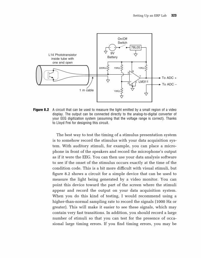
The best way to test the timing of a stimulus presentation system
is to somehow record the stimulus with your data acquisition sys-
tem. With auditory stimuli, for example, you can place a micro-
phone in front of the speakers and record the microphone’s output
as if it were the EEG. You can then use your data analysis software
to see if the onset of the stimulus occurs exactly at the time of the
condition code. This is a bit more difficult with visual stimuli, but
figure 8.2 shows a circuit for a simple device that can be used to
measure the light being generated by a video monitor. You can
point this device toward the part of the screen where the stimuli
appear and record the output on your data acquisition system.
When you do this kind of testing, I would recommend using a
higher-than-normal sampling rate to record the signals (1000 Hz or
greater). This will make it easier to see these signals, which may
contain very fast transitions. In addition, you should record a large
number of stimuli so that you can test for the presence of occa-
sional large timing errors. If you find timing errors, you may be
3–
–
+
+
8
10KΩ
LM311
9VBattery
On/OffSwitch
L14 Phototransistorinside tube withone end open
1 m cable
78L05
To ADC +
To ADC –2 14
7
15KΩ220KΩ 10KΩ
Figure 8.2 A circuit that can be used to measure the light emitted by a small region of a videodisplay. The output can be connected directly to the analog-to-digital converter ofyour EEG digitization system (assuming that the voltage range is correct). Thanksto Lloyd Frei for designing this circuit.
Setting Up an ERP Lab 323

able to eliminate them by disabling any unnecessary hardware and
software systems on the computer. For example, you can make
sure that no other programs or operating system extensions are
running in parallel on the computer, and you can disconnect the
computer from networks, unnecessary hard drives, printers, and
so on.
Stimulus-Related Artifacts
Whatever stimuli you use, you should make sure they will not
cause electrical artifacts that will be picked up by the electrodes
or cause reflexes that will contaminate the data. For example, most
audio headphones operate by passing a current through a coil to
cause the movement of a membrane with respect to a magnet, and
this can induce a current in the electrodes. Thus, shielded head-
phones may be important for auditory ERP studies. In addition,
sudden noises can elicit a muscle twitch called the post-auricular
reflex, which the EEG electrodes can pick up. Somatosensory stim-
ulation is most often produced with small shocks, and these can
also induce artifacts in the electrodes and elicit reflexes.
Stimulus Timing on CRTs
The remainder of this chapter will focus on presenting visual stim-
uli on a computer-controlled cathode-ray tube (CRT) monitor (see
Brainard, Pelli, & Robson, 2002 for a more detailed discussion).
There are three reasons for focusing on visual stimuli. First, visual
stimuli are used much more commonly than stimuli in other modal-
ities. Second, the presentation of visual stimuli on a CRT involves
some subtle timing issues that are particularly important in ERP
experiments. Finally, I just don’t have much experience with stim-
uli in other modalities, so I can’t provide much detailed informa-
tion. You can learn about the details of non-visual stimulation
from the literature or by asking experts.
Chapter 8 324
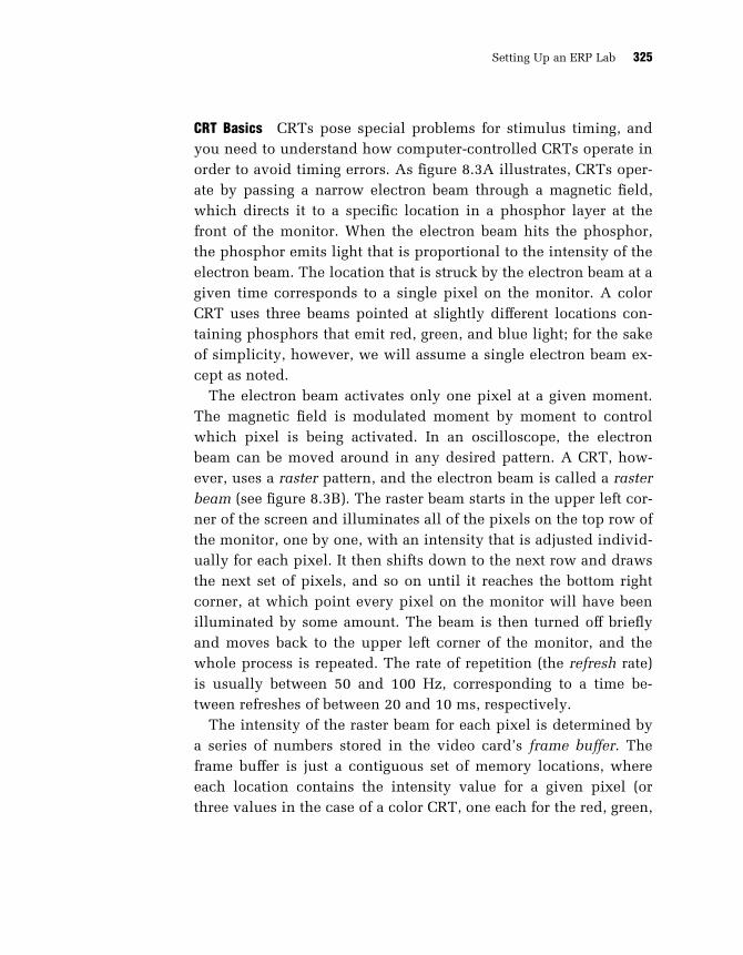
CRT Basics CRTs pose special problems for stimulus timing, and
you need to understand how computer-controlled CRTs operate in
order to avoid timing errors. As figure 8.3A illustrates, CRTs oper-
ate by passing a narrow electron beam through a magnetic field,
which directs it to a specific location in a phosphor layer at the
front of the monitor. When the electron beam hits the phosphor,
the phosphor emits light that is proportional to the intensity of the
electron beam. The location that is struck by the electron beam at a
given time corresponds to a single pixel on the monitor. A color
CRT uses three beams pointed at slightly different locations con-
taining phosphors that emit red, green, and blue light; for the sake
of simplicity, however, we will assume a single electron beam ex-
cept as noted.
The electron beam activates only one pixel at a given moment.
The magnetic field is modulated moment by moment to control
which pixel is being activated. In an oscilloscope, the electron
beam can be moved around in any desired pattern. A CRT, how-
ever, uses a raster pattern, and the electron beam is called a raster
beam (see figure 8.3B). The raster beam starts in the upper left cor-
ner of the screen and illuminates all of the pixels on the top row of
the monitor, one by one, with an intensity that is adjusted individ-
ually for each pixel. It then shifts down to the next row and draws
the next set of pixels, and so on until it reaches the bottom right
corner, at which point every pixel on the monitor will have been
illuminated by some amount. The beam is then turned off briefly
and moves back to the upper left corner of the monitor, and the
whole process is repeated. The rate of repetition (the refresh rate)
is usually between 50 and 100 Hz, corresponding to a time be-
tween refreshes of between 20 and 10 ms, respectively.
The intensity of the raster beam for each pixel is determined by
a series of numbers stored in the video card’s frame buffer. The
frame buffer is just a contiguous set of memory locations, where
each location contains the intensity value for a given pixel (or
three values in the case of a color CRT, one each for the red, green,
Setting Up an ERP Lab 325

Magnets
Phosphor
ElectronBeam
A
B
C
0 50
Time (ms)
Pixel in upperleft corner
Pixel in lowerright cornerP
ixel
Inte
nsity
100 150
Figure 8.3 Operation of a CRT monitor. (A) The electron beam is directed by a magnetic field toa specific location at the front of the monitor, causing a small spot in the phosphorlayer to become illuminated. (B) Raster pattern of the movement of the electronbeam over time. (C) Intensity of the luminance from pixels on two different locationson a CRT monitor.
Chapter 8 326

and blue intensities). When a program draws an image to the mon-
itor, it is really just updating values in the frame buffer. No change
occurs on the monitor until the raster beam reaches the set of pix-
els corresponding to the updated values, at which point the values
are read from the frame buffer and the pixels are activated accord-
ingly. This is a big part of why timing is so tricky for CRTs: the
time at which something actually appears on the screen is deter-
mined by both the contents of the frame buffer, which your pro-
gram directly controls, and the position of the raster beam, which
your program does not directly control.
CRT Timing As illustrated in figure 8.3C, a pixel’s intensity
increases almost instantaneously when the raster beam hits the
phosphor, and then the intensity falls fairly rapidly toward zero
when the raster beam moves away As an example, consider a sce-
nario in which the refresh rate is set at 60 Hz (16.67 ms per re-
fresh), the raster beam starts at the upper left corner at time zero,
and the entire screen is to be turned on at 50 ms, remain visible
for 50 ms, and then be turned off. The top trace in figure 8.3C
shows the intensity of the pixel at the top left corner of the screen
for this scenario. The intensity of the raster beam will be low when
it hits this pixel at times 0, 16.67 ms, and 33.33 ms, and then tran-
sition to high when it hits the pixel at times 50, 66.67, and 83.33
ms, returning again to a low value at 100 ms. The pixel’s illumina-
tion will spike upward at these times and then decay downward in
the intervening periods. We don’t perceive it as flickering, how-
ever, because the retina integrates information over time.1
Less than a microsecond after the pixel in the upper left corner is
illuminated at 50 ms, the next pixel to the right will be illumi-
nated, and then the next one, and so on until the entire top row
has been illuminated (drawing one row of pixels will take approxi-
mately 120 ms with a 640 480 resolution). The pixels in the next
row will then be sequentially illuminated, and then the next row,
and so on until the entire display has been illuminated (which
Setting Up an ERP Lab 327

will take approximately 16 ms with a 60-Hz refresh rate). The bot-
tom trace in figure 8.3C shows the actual illumination that would
be observed for a pixel near the bottom of the display. The illumi-
nation of this pixel is delayed by approximately 16 ms compared
to the pixel in the upper left hand corner of the display. Thus, the
display is not drawn in a single instant, but instead is gradually
painted over a period of many milliseconds.
Timing Errors If your stimulus presentation program draws an ob-
ject at some random time, it may cause a large, visible artifact
known as tearing. This happens when the frame buffer is being
updated in the same set of locations that are currently being drawn
to the display by the raster beam. It is important to avoid this arti-
fact, which can be very distracting.
To avoid tearing and permit precise timing, video cards send a
signal to the computer called a vertical retrace interrupt or video
blanking interrupt just after the raster beam has finished a cycle of
drawing and just before the next cycle is about to begin. In most
cases, the best way to ensure correct timing is to use the following
sequence of events in the stimulus presentation program: (a) wait
for the interrupt signal, (b) send an event code, and (c) draw the
stimuli in a manner that ensures that any changes in the intensity
values stored by the frame buffer occur after the interrupt but be-
fore those values are read by the raster beam.
By following this sequence, you can be sure that your event code
is linked to the position of the electrode beam and therefore to the
moment at which the illumination of the monitor actually changes.
There will be a delay between the event code and the illumination
of a given pixel, and this delay will depend on the location of the
pixel (i.e., it will be larger for lower rows than for higher rows).
However, this delay is constant for a given location, and you can
determine the amount of delay by recording the illumination at a
given location with the device shown in figure 8.2C. A known,
constant delay is a minor annoyance, whereas an unknown, vari-
able delay can be a major problem.
Chapter 8 328

The tricky part of this sequence is the last part, making sure that
you do not change values in the frame buffer after those values
have already been used to control the raster beam on a given raster
cycle. There are two common ways this can occur. First, if you are
drawing a complex stimulus or have a slow computer or software
system, it may take longer than one raster cycle to draw the stimu-
lus. Second, you may not draw from top to bottom, and a portion of
the stimulus display may be drawn to the frame buffer after the
raster beam has already drawn this portion of the display. For ex-
ample, imagine you are conducting a visual search experiment in
which twenty-four squares are drawn at random locations across
the display. If you wait for the vertical retrace interrupt and then
start drawing the squares to the frame buffer in random order, you
may end up drawing a square near the top of the frame buffer 5 ms
after the interrupt. By this point, the raster beam will have already
drawn the top portion of the frame buffer, so you may see tearing
artifacts, and the square will not appear until early in the next
raster cycle.
In most cases, the best way to avoid these problems is to predraw
each stimulus display in an offscreen memory buffer. That is, prior
to each trial of the experiment, you can predraw the stimulus dis-
plays in an area of memory that simulates the frame buffer but is
not actually visible. When it is time to display the stimulus, you
will wait for the vertical retrace interrupt, send an event code, and
then copy the simulated frame buffer into the actual frame buffer.
As long as the copying is done from top to bottom and is faster
than the raster beam, this will guarantee that your timing is per-
fectly precise (although pixels near the bottom of the display will
still be illuminated later than pixels near the top of the display).
Alternatively, some video cards contain multiple frame buffers,
and it is possible to predraw the stimuli in one frame buffer while
another frame buffer is being displayed. The predrawn frame buffer
can then be displayed by telling the video card to switch the
displayed location, which is virtually instantaneous. No copying
from memory into the frame buffer is necessary in this case.
Setting Up an ERP Lab 329

Software Packages Various stimulus presentation programs are
available, and some are designed expressly for use in ERP experi-
ments. Before purchasing a program, you should inquire about the
nature of the video timing. Every vendor will tell you that the tim-
ing is accurate, but you should find out exactly how the program
works. In particular, you should find out whether the program (a)
synchronizes stimulus presentation and event codes to the vertical
retrace interrupt, (b) predraws each display to an offscreen memory
buffer, and (c) might be occasionally interrupted by other programs
or the operating system, which may cause large timing errors.
If you are inclined to write your own visual stimulus presenta-
tion programs, I would highly recommend using MATLAB and a
set of routines called the PsychToolbox. This toolbox was devel-
oped by two highly respected vision researchers, David Brainard
and Dennis Pelli (Brainard, 1997; Pelli, 1997), and they have rigor-
ously tested its timing. MATLAB provides an excellent environ-
ment for the relatively rapid development of new experiments,
and the PsychToolbox makes it easy to implement the sequence of
procedures described here.
CRTs versus LCDs At the time of this writing, CRT monitors are
quickly being displaced by LCD monitors, and this change may ob-
viate much of the information provided so far. Unfortunately, LCD
technology has not stabilized enough for me to provide useful in-
formation about how to achieve precise timing with LCDs.
LCD displays operate by using electrical signals to change the
polarization of display elements, which in turn influences the trans-
mission of light. No raster beam is necessary, so LCDs can poten-
tially make instantaneous changes to pixels in any position on the
screen. However, LCDs are being integrated into computer systems
that were originally designed with CRTs in mind, and information
from the video card’s frame buffer is typically transmitted serially
to the LCD display. Thus, it is still important to consider carefully
the timing of the stimuli with respect to the event codes.
The optical properties of LCDs can also be problematic. In the
context of ERP recordings, the biggest problem is that the trans-
Chapter 8 330

mission of light by LCDs changes relatively slowly. As a result,
stimulus onsets and offsets will be more gradual than on CRTs.
Fortunately, LCD manufacturers are motivated to reduce this prob-
lem because of the growing use of LCDs for television displays,
video games, and other high-speed applications. Thus, LCDs may
soon have better temporal properties.
To examine LCD timing firsthand, I used the circuit shown in fig-
ure 8.2 to measure the output of a high quality LCD monitor, and I
recorded this signal with an ERP digitization system. Rather than
using a digital LCD interface, I connected the LCD display to the
computer’s analog VGA output, which is designed for CRTs. Most
current LCDs have both analog and digital inputs, and the digital
350 400 450
Time after Event Code (ms)
300
200 400 600
Time after Event Code (ms)
0
A
20 40 60
Time after Event Code (ms)
0
B
C
LCD
Lum
inan
ceLC
DLu
min
ance
LCD
Lum
inan
ce
Figure 8.4 Luminance recorded from an LCD monitor in response to a white square presentedon a black background. The same luminance signal is shown on three different timescales.
Setting Up an ERP Lab 331
input will usually have higher fidelity (but may have unknown
timing properties). Figure 8.4 illustrates the output of the LCD at
the location of a white square that was presented on a black back-
ground. The square was supposed to onset at 0 ms (the time of the
event code) and offset at 350 ms (and this is exactly what would
have happened if I had used a CRT monitor).
Figure 8.4A shows the entire time course of the LCD output; the
onset and offset appear on expanded time scales in figures 8.4B
and 8.4C, respectively. The figure illustrates three potential prob-
lems with LCDs. First, the LCD’s output is slightly delayed: The
onset of the luminance change does not begin until approximately
7 ms after the event code, and the luminance does not begin to de-
cline until approximately 357 ms. I suspect that this is caused by
the analog VGA connection; the analog signal must be converted
back into a digital form by the LCD monitor. Second, the onset is
not instantaneous, but instead builds up over a period of approxi-
mately 5 ms. This is probably fast enough for the majority of ERP
experiments, but this particular LCD display was chosen for its
rapid onset time, and other LCD displays ramp up over a substan-
tially longer period. Third, the offset of the display is very gradual,
requiring almost 100 ms to reach the baseline luminance value.
This won’t be a significant problem when stimuli are presented on
a black background. However, if the stimuli are presented on a
white background, the onset of a stimulus will be achieved by a de-
crease in luminance, and the luminance will change in the slow
manner shown in figure 8.4C. This could be quite problematic for
experiments in which precise timing is important.
LCDs do have a very significant advantage over CRTs: They don’t
pump a stream of electrons directly toward the subject’s head. Con-
sequently, LCDs should produce less electrical noise than CRTs,
and a Faraday cage may not be necessary. LCDs may therefore be-
come the best choice for most experiments once the technology
reaches maturity. In the meantime, you may wish to try using LCD
monitors, but you should carefully test the timing of an each dis-
play before using it (different models may have radically different
temporal properties).
Chapter 8 332

Appendix: Basic Principles of Electricity
This appendix describes some important aspects of electricity and
magnetism that arise when considering the neural origins of ERPs
and sources of noise that can arise in ERP recordings.
Electricity is simply the flow of charges through a conductive
medium. In electrical circuits, it is usually electrons that actually
flow. In the nervous system, much of the electricity is due to the
movement of small ions across cell membranes. But the principles
of electricity are the same in both of these situations.
Voltage, Current, and Resistance
The three most fundamental terms in electricity are voltage, cur-
rent, and resistance. Voltage is essentially electrical pressure and
is analogous water pressure. Voltage is also called electrical poten-
tial, because it reflects the potential for electrical current to flow
from one place to another. This can be understood by analogy to
the flow of water through pipes. Consider, for example, a tank of
water at the top of a hill. There is a lot of potential for the water to
flow to the bottom of the hill, but little potential for the water to
float up to the top. Importantly, the potential for water to flow
downhill is present even if no water is flowing at a given moment
(e.g., because a valve is closed). Similarly, there is potential for
electrical current to flow from one terminal of a car battery to the
other even if no current is flowing. Voltage is usually labeled E for
electromotive force.
Current is the number of charged particles (e.g., electrons) that
flow past a given point in a specific amount of time. Current is
measured in amperes, where 1 ampere is equal to 1 coulomb

(6:24 1018) of charges moving past a single point in one second.
Measuring electrical current is analogous to measuring the quan-
tity of water that passes through a given segment of pipe in a fixed
time period (e.g., 10 liters per minute). Current is usually labeled I
for intensity.
Resistance is the ability of a substance to keep charged particles
from passing (it’s the inverse of conductance). Three main factors
contribute to resistance: (1) the composition of the substance, (2)
its length, and (3) its diameter. Due to their molecular properties,
some substances conduct electricity better than others (e.g., copper
is a better conductor than zinc). However, the ability of any sub-
stance to conduct electricity will be reduced if it is very thin. To
use yet another hydraulic example, consider a water filtration sys-
tem in which the water supply for a house passes through a large
tank filled with carbon. If the carbon is tightly packed, water will
not easily flow through the tank, but if the carbon is loosely
packed, water will flow easily. This is analogous to the depen-
dence of electrical resistance on the properties of the substance.
Now imagine water passing through a hose. If the hose is very
long and narrow, a great deal of pressure will be necessary to fill a
bucket in a short amount of time; if the hose is short and wide, the
bucket will fill quickly with only a moderate amount of water pres-
sure. This is analogous to the dependence of electrical resistance
on the length and diameter of the conductor. Resistance is mea-
sured in Ohms (W) and is usually labeled R.
This last analogy also illustrates the relationships among voltage,
current, and resistance. If a thin hose is used, the volume of water
that passes out of the end of the hose will be small relative to what
would be obtained with a wider hose and the same water pressure.
Similarly, if voltage stays the same and the resistance increases,
the current will decrease. However, if a thin hose is used, a large
volume of water can be obtained in a given time period by increas-
ing the water pressure. Similarly, it is possible to maintain a con-
stant current when the resistance is increased by increasing the
voltage.
Appendix: Basic Principles of Electricity 334

Ohm’s Law
These relationships are summarized by Ohm’s law: E ¼ IR (volt-
age is equal to the product of the current and the resistance). This
means that 1 volt of electromotive force is required to pass 1 am-
pere of current through a resistance of 1 ohm. This equation
implies that if the voltage is increased, then this must be accom-
panied by an increase in current, an increase in resistance, or
changes in both current and resistance. In particular, if the voltage
increases and the resistance is constant, then the current must in-
crease in proportion with the voltage. This makes sense, because
an increase in the pressure (voltage) naturally leads to an increase
in current. However, a somewhat less intuitive consequence of
Ohm’s law is that if the resistance increases and the current is
held constant, then the voltage must increase in proportion to the
resistance. This might seem counterintuitive, because you might
expect that an increase in resistance would lead to a decrease in
voltage, but it actually leads to an increase in voltage (assuming
that current remains constant). However, this makes sense if you
think about the hydraulic analogy: If you use a thinner hose but
still have the same amount of water coming out the end, you must
have increased the water pressure.
Another implication of Ohm’s law is that it is possible to have a
very large voltage without any significant current if the resistance
is near infinity, which is very common (as in the case of the termi-
nals of a car battery when they are not connected to anything).
However, the only way to get a significant current without any sig-
nificant voltage is to have a resistance that is near zero, which is
very uncommon (it requires supercooling).
Impedance
There is one other term that I would like to mention in this con-
text, namely impedance. Technically, the term resistance applies
only when the current is constant over time (which is called direct
current or DC), and impedance is the appropriate term to use when
Appendix: Basic Principles of Electricity 335

the current varies over time (alternating current or AC). Because
ERPs vary over time, impedance is generally the most relevant
concept. A different term is necessary because there are certain
factors that contribute to impedance that do not contribute to DC
resistance (specifically, inductance and capacitance). However, for
most practical purposes, impedance is analogous to resistance, so
you don’t need to worry about the differences. Impedance is usu-
ally labeled Z, and most impedance meters measure the impedance
using a small sine-wave voltage oscillating at around 10 Hz.
Electricity and Magnetism
Electricity and magnetism are fundamentally related to each other,
and it is important to understand this relationship to understand
how ERP recordings pick up electrical noise and how MEG/ERMF
recordings are related to EEG/ERP recordings. Current flowing
through a conductor generates a magnetic field that flows around
the conductor. Moreover, if a magnetic field passes through a con-
ductor, it induces an electrical current. Figure A.1 illustrates these
Current flowsthrough conductor #1
Magnetic fieldinduces current flow
in conductor #2
Magnetic fieldgenerated around
conductor #1
Conductor #1
Conductor #2
Figure A.1 Relationship between electricity and magnetism. A current is passed throughconductor #1, and this generates a magnetic field that circles around conductor #1.As this magnetic field passes through conductor #2, it induces a small current inconductor #2.
Appendix: Basic Principles of Electricity 336

two principles, showing what happens when a current passes
through one of two nearby conductors. The flow of current through
one of the conductors generates a magnetic field, which in turn
induces current flow in the other conductor. This is how electrical
noise in the environment can induce electrical activity in an ERP
subject, in the electrodes, or in the wires leading from the elec-
trodes to the amplifier.
Appendix: Basic Principles of Electricity 337


Notes
Chapter 1
1. The concept of noise is fundamental to any data recording technique, but this term is un-
familiar to many beginners. The term noise simply refers to any source of variation in the
data that is unrelated to thing you are trying to record (which is termed the signal). Keep
in mind that one researcher’s noise may be another researcher’s signal. For example, elec-
trical activity generated by the heart (the EKG) may sometimes contaminate ERP record-
ings, and ERP researchers treat it as noise. To a cardiologist, however, the EKG is a signal,
not noise. Noise may be random and unpredictable or it may be nonrandom and predict-
able. As long as it causes the recorded data to differ from the signal, however, it’s still
noise.
2. This assumes that the recording electrode is at a sufficient distance from the activated
cortex, which will always be true in scalp recordings.
3. To be more precise, the high resistance of the skull causes a small amount of volume-
conducted electrical current to flow perpendicular to the skull, and this perpendicular
electrical activity is accompanied by a small magnetic field. In this manner, the high re-
sistance of the skull may indirectly cause a small amount of distortion in magnetic fields.
However, this is a relatively minor effect compared to the distortion of the electrical
activity.
4. You may wonder why all this research has not led to a consensus about the psychological
or neurophysiological processes reflected by the P3 wave. I suspect there are two main
contributing factors. One factor is that the P3 wave is present, at least to some extent, in
almost every condition of almost every experiment. Because the P3 wave is so ubiquitous,
it’s hard to narrow down the general cognitive domain associated with it. A second factor
is that it’s difficult to isolate the P3 wave from other overlapping ERP components.
It seems very likely that many different positive-going ERP components are active over
the broad time range and scalp distribution of the P3 wave, each reflecting a different
cognitive process. Because we don’t have a good means of isolating these different P3
subcomponents, it’s very hard to associate this amalgam of P3 activity with a specific psy-
chological process.
Chapter 2
1. An abbreviated version of this chapter has been published previously (Luck, 2005).
2. This definition has a bit of wiggle room in the definition of a neuroanatomical module.
You could use Brodmann’s areas to define the modules, but you could also use the finer

divisions of modern neuroanatomy (Felleman & Van Essen, 1991) or coarser divisions
such as the dorsal stream or the ventral stream.
3. The results in the figure are summarized in a bar graph, and ERP waveforms are not
shown. Because it is difficult to measure the latent components from the observed ERP
waveforms, it is important to show the ERP waveforms and not just provide measure-
ments of component amplitudes and latencies (see the first section of chapter 6 for more
details). However, at the time of this experiment, computers were quite primitive, and
computing something as straightforward as the average waveform across subjects was
not terribly common. The original journal article describing this experiment did not con-
tain any grand averages, and instead showed examples of the waveforms from a few sub-
jects. The individual-subject waveforms were just too ugly to show here.
Chapter 4
1. Technically speaking, covariance is used rather than correlation, which means that the
matching EEG segment must be large as well as being similar in shape to the template.
2. The data shown in this figure were actually computed using a somewhat different tech-
nique, which used wavelet transforms instead of Fourier transforms. However, the gen-
eral principle is the same.
3. This framework was originally developed by Jon Hansen at UCSD. He also developed sev-
eral of the specific artifact rejection algorithms described later in this chapter.
4. Although a chinrest seems like it ought to reduce muscle tension, my lab has found that
they actually increase muscle noise. But it may be possible to set up a chinrest in a way
that reduces rather than increases muscle noise.
Chapter 5
1. In this context, power is simply amplitude squared.
2. The discussion of filtering presented here applies to transient waveforms from virtually
any source, including event-related magnetic fields. However, these principles are rele-
vant primarily for the transient responses that are elicited by discrete stimuli and not to
the steady-state responses that are elicited by fast, repetitive streams of stimuli presented
at a constant rate.
3. Plots of phase are often difficult to understand, and the Fourier transforms shown in
this chapter will show the amplitude information without the corresponding phase
information.
4. The process is actually somewhat more complex than this due to the fact that both the
ERP waveform and the impulse response function are finite in duration and digitally
sampled.
5. A 12.5-Hz half-amplitude cutoff is much lower than the cutoff frequencies typically
employed for attenuating high frequency noise. However, filter-induced distortions are
more apparent in this context with lower cutoffs, and a 12.5 Hz cutoff was therefore
chosen to make these distortions clearer.
6. Artifact rejection is a nonlinear process, and filtering before artifact rejection and
averaging will not yield the same result as filtering after artifact rejection and averaging
Notes 340

(although the result will be very similar if the specific filter used doesn’t influence the
artifact rejection process very much).
Chapter 6
1. Occasionally, the waveform will not have a local peak within the measurement time
range that exceeds the average of the three to five points on either side. This occurs
when the waveform gradually increases or decreases monotonically through the entire
measurement window. In this case, you can just use the simple peak amplitude or the
amplitude at the midpoint of the latency range. These aren’t perfect solutions, but they’re
better than always using the simple peak amplitude.
2. The Greenhouse-Geisser adjustment tends to be overly conservative, especially at moder-
ate to high levels of non-sphericity. Many statistical packages also include the Hyun-
Feldt adjustment, which is probably somewhat more reasonable and may be useful when
low statistical power is a problem.
Chapter 7
1. A physicist with no knowledge of BESA or ERPs was also tested, but his localizations
were both unrepresentative and far from correct, so I will not include his results in the
discussion here.
2. If two dipoles are assumed to be mirror-symmetrical, only seven parameters are
required to represent the two dipoles, rather than the twelve that would be otherwise
required. That is, six parameters are used to represent one of the two dipoles, as usual,
but the other dipole requires only one additional parameter, representing its magnitude
(which is the only parameter that may differ from the other dipole). Moreover, because
magnitude is treated differently from the other parameters in BESA, the assumption of
mirror symmetry essentially removes all of the major parameters from one of the two
dipoles. Thus, this ten-dipole simulation is equivalent to an unconstrained seven-dipole
simulation.
Chapter 8
1. Because of the integration time of the retina, reducing the duration of a stimulus from 100
ms to some shorter duration leads to the perception of a dimmer stimulus rather than a
shorter stimulus (this is Bloch’s law). In addition, stimuli of approximately 100 ms or
less do not elicit separate onset and offset ERP responses, but longer stimuli do. Con-
sequently, I would recommend a duration of 100 ms for experiments with brief stimuli,
and I would recommend a duration that exceeds the interesting portion of the ERP wave-
form for experiments with long stimuli. This way you will not have offset responses in
the middle of your waveform.
Notes 341


References
Adrian, E. D., & Matthews, B. H. C. (1934). The Berger rhythm: Potential changes from the
occipital lobes in man. Brain, 57, 355–385.
Aine, C., Huang, M., Stephen, J., & Christner, R. (2000). Multistart algorithms for MEG
empirical data analysis reliably characterize locations and time courses of multiple
sources. Neuroimage, 12, 159–172.
Alcaini, M., Giard, M. H., Thevenet, M., & Pernier, J. (1994). Two separate frontal compo-
nents in the N1 wave of the human auditory evoked response. Psychophysiology, 31,
611–615.
American Encephalographic Society. (1994). Guidelines for standard electrode position
nomenclature. Journal of Clinical Neurophysiology, 11, 111–113.
Baillet, S., Mosher, J. C., Leahy, R. M., & Shattuck, D. W. (1999). BrainStorm: A matlab
toolbox for the processing of MEG and EEG signals. Neuroimage, 9, 246.
Bentin, S., Allison, T., Puce, A., Perez, E., & McCarthy, G. (1996). Electrophysiological
studies of face perception in humans. Journal of Cognitive Neuroscience, 8, 551–565.
Bentin, S., & Carmel, D. (2002). Accounts for the N170 face-effect: A reply to Rossion,
Curran, & Gauthier. Cognition, 85, 197–202.
Berg, P., & Scherg, M. (1991a). Dipole modelling of eye activity and its application to the
removal of eye artefacts from the EEG and MEG. Clinical Physics & Physiological
Measurement, 12 Suppl A, 49–54.
Berg, P., & Scherg, M. (1991b). Dipole models of eye movements and blinks. Electroence-
phalography & Clinical Neurophysiology, 79, 36–44.
Berg, P., & Scherg, M. (1994). A multiple source approach to the correction of eye arti-
facts. Electroencephalography & Clinical Neurophysiology, 90, 229–241.
Berger, H. (1929). Ueber das Elektrenkephalogramm des Menschen. Archives fur Psychia-
trie Nervenkrankheiten, 87, 527–570.
Bertrand, O., Perrin, F., & Pernier, J. (1991). Evidence for a tonotopic organization of the
auditory cortex with auditory evoked potentials. Acta Otolaryngologica, 491, 116–
123.
Brainard, D. H. (1997). The psychophysics toolbox. Spatial Vision, 10, 433–436.
Brainard, D. H., Pelli, D. G., & Robson, T. (2002). Display characterization. In J. Hornak
(Ed.), Encyclopedia of Imagine Science and Technology (pp. 172–188). New York:
Wiley.
Brandeis, D., Naylor, H., Halliday, R., Callaway, E., & Yano, L. (1992). Scopolamine
effects on visual information processing, attention, and event-related potential map
latencies. Psychophysiology, 29, 315–336.
Broadbent, D. E. (1958). Perception and Communication. New York: Pergamon.
Carmel, D., & Bentin, S. (2002). Domain specificity versus expertise: Factors influencing
distinct processing of faces. Cognition, 83, 1–29.

Chelazzi, L., Duncan, J., Miller, E. K., & Desimone, R. (1998). Responses of neurons in
inferior temporal cortex during memory-guided visual search. Journal of Neurophysi-
ology, 80, 2918–2940.
Chelazzi, L., Miller, E. K., Duncan, J., & Desimone, R. (1993). A neural basis for visual
search in inferior temporal cortex. Nature, 363, 345–347.
Chelazzi, L., Miller, E. K., Duncan, J., & Desimone, R. (2001). Responses of neurons in ma-
caque area V4 during memory-guided visual search. Cerebral Cortex, 11, 761–772.
Chun, M. M., & Potter, M. C. (1995). A two-stage model for multiple target detection in
rapid serial visual presentation. Journal of Experimental Psychology: Human Percep-
tion and Performance, 21, 109–127.
Clark, V. P., Fan, S., & Hillyard, S. A. (1995). Identification of early visually evoked poten-
tial generators by retinotopic and topographic analyses. Human Brain Mapping, 2,
170–187.
Cohen, D., & Cuffin, B. N. (1991). EEG versus MEG localizaiton accuracy: Theory and
experiment. Brain Topography, 4, 95–103.
Coles, M. G. H. (1989). Modern mind-brain reading: Psychophysiology, physiology and
cognition. Psychophysiology, 26, 251–269.
Coles, M. G. H., Gratton, G., Kramer, A. F., & Miller, G. A. (1986). Principles of signal
acquisition and analysis. In M. G. H. Coles, E. Donchin & S. W. Porges (Eds.), Psycho-
physiology: Systems, Processes, and Applications (pp. 183–221). New York: Guilford
Press.
Coles, M. G. H., & Rugg, M. D. (1995). Event-related potentials: An introduction. In M. D.
Rugg & M. G. H. Coles (Eds.), Electrophysiology of Mind (pp. 1–26). New York:
Oxford University Press.
Coles, M. G. H., Smid, H., Scheffers, M. K., & Otten, L. J. (1995). Mental chronometry and
the study of human information processing. In M. D. Rugg & M. G. H. Coles (Eds.),
Electrophysiology of Mind: Event-Related Brain Potentials and Cognition (pp. 86–
131). Oxford: Oxford University Press.
Courchesne, E., Hillyard, S. A., & Galambos, R. (1975). Stimulus novelty, task relevance
and the visual evoked potential in man. Electroencephalography and Clinical Neuro-
physiology, 39, 131–142.
Cuffin, B. N., Cohen, D., Yunokuchi, K., Maniewski, R., Purcell, C., Cosgrove, G. R., Ives,
J., Kennedy, J., & Schomer, D. (1991). Test of EEG localization accuracy using
implanted sources in the human brain. Annals of Neurology, 29, 132–138.
Dale, A. M., & Sereno, M. I. (1993). Improved localization of cortical activity by combin-
ing EEG and MEG with MRI cortical surface reconstruction: A linear approach. Jour-
nal of Cognitive Neuroscience, 5, 162–176.
Davis, H., Davis, P. A., Loomis, A. L., Harvey, E. N., & Hobart, G. (1939). Electrical reac-
tions of the human brain to auditory stimulation during sleep. Journal of Neurophysi-
ology, 2, 500–514.
Davis, P. A. (1939). Effects of acoustic stimuli on the waking human brain. Journal of
Neurophysiology, 2, 494–499.
de Jong, R., Coles, M. G., Logan, G. D., & Gratton, G. (1990). In search of the point of
no return: The control of response processes. Journal of Experimental Psychology:
Human Perception & Performance, 16, 164–182.
Dehaene, S., Naccache, L., Le Clec, H. G., Koechlin, E., Mueller, M., Dehaene-Lambertz,
G., van de Moortele, P. F., & Le Bihan, D. (1998). Imaging unconscious semantic pri-
ming. Nature, 395, 597–600.
References 344

Dehaene, S., Posner, M. I., & Tucker, D. M. (1994). Localization of a neural system for
error detection and compensation. Psychological Science, 5, 303–305.
Delorme, A., & Makeig, S. (2004). EEGLAB: An open source toolbox for analysis of single-
trial EEG dynamics including independent component analysis. Journal of Neuro-
science Methods, 134, 9–21.
Desmedt, J. E., Chalklin, V., & Tomberg, C. (1990). Emulation of somatosensory evoked
potential (SEP) components with the 3-shell head model and the problem of ‘‘ghost
potential fields’’ when using an average reference in brain mapping. Electroencepha-
lography & Clinical Neurophysiology, 77, 243–258.
Deutsch, J. A., & Deutsch, D. (1963). Attention: Some theoretical considerations. Psycho-
logical Review, 70, 80–90.
Di Russo, F., Martinez, A., Sereno, M. I., Pitzalis, S., & Hillyard, S. A. (2002). Cortical
sources of the early components of the visual evoked potential. Human Brain Map-
ping, 15, 95–111.
Di Russo, F., Teder-Salejarvi, W. A., & Hillyard, S. A. (2003). Steady-state VEP and atten-
tional visual processing. In A. Zani & A. M. Proverbio (Eds.), The Cognitive Electro-
physiology of Mind and Brain (pp. 259–274). San Diego: Academic Press.
Dien, J. (1998). Issues in the application of the average reference: Review, critiques, and
recommendations. Behavior Research Methods, Instruments, & Computers, 30, 34–
43.
Donchin, E. (1981). Surprise! . . . Surprise? Psychophysiology, 18, 493–513.
Donchin, E. (1979). Event-related brain potentials: A tool in the study of human informa-
tion processing. In H. Begleiter (Ed.), Evoked Brain Potentials and Behavior (Vol. 2,
pp. 13–88). New York: Plenum Press.
Donchin, E., & Coles, M. G. H. (1988). Is the P300 component a manifestation of context
updating? Behavioral Brain Science, 11, 357–374.
Donchin, E., & Heffley, E. F., III. (1978). Multivariate analysis of event-related potential
data: A tutorial review. In D. Otto (Ed.), Multidisciplinary Perspectives in Event-
Related Brain Potential Research (pp. 555–572). Washington, D.C.: U.S. Government
Printing Office.
Duncan-Johnson, C., & Donchin, E. (1979). The time constant in P300 recording. Psycho-
physiology, 16, 53–55.
Duncan-Johnson, C. C., & Donchin, E. (1977). On quantifying surprise: The variation
of event-related potentials with subjective probability. Psychophysiology, 14, 456–
467.
Duncan-Johnson, C. C., & Kopell, B. S. (1981). The Stroop effect: Brain potentials localize
the source of interference. Science, 214, 938–940.
Eimer, M. (1996). The N2pc component as an indicator of attentional selectivity. Electro-
encephalography and Clinical Neurophysiology, 99, 225–234.
Eriksen, C. W., & Schultz, D. W. (1979). Information processing in visual search: A con-
tinuous flow conception and experimental results. Perception and Psychophysics,
25, 249–263.
Falkenstein, M., Hohnsbein, J., Joormann, J., & Blanke, L. (1990). Effects of errors in
choice reaction tasks on the ERP under focused and divided attention. In C. H. M.
Brunia, A. W. K. Gaillard & A. Kok (Eds.), Psychophysiological Brain Research (pp.
192–195). Amsterdam: Elsevier.
Felleman, D. J., & Van Essen, D. C. (1991). Distributed hierarchical processing in the pri-
mate cerebral cortex. Cerebral Cortex, 1, 1–47.
References 345

Ferree, T. C., Luu, P., Russell, G. S., & Tucker, D. M. (2001). Scalp electrode impedance,
infection risk, and EEG data quality. Clinical Neurophysiology, 112, 536–544.
Gaillard, A. W. K. (1988). Problems and paradigms in ERP research. Biological Psychol-
ogy, 26, 91–109.
Galambos, R., & Sheatz, G. C. (1962). An electroencephalographic study of classical con-
ditioning. American Journal of Physiology, 203, 173–184.
Ganis, G., Kutas, M., & Sereno, M. I. (1996). The search for ‘‘common sense’’: An electro-
physiological study of the comprehension of words and pictures in reading. Journal
of Cognitive Neuroscience, 8, 89–106.
Garner, W. R., Hake, H. W., & Eriksen, C. W. (1956). Operationism and the concept of per-
ception. Psychology Review, 63, 149–159.
Gehring, W. J., Goss, B., Coles, M. G. H., Meyer, D. E., & Donchin, E. (1993). A neural sys-
tem for error-detection and compensation. Psychological Science, 4, 385–390.
Gehring, W. J., & Willoughby, A. R. (2002). The medial frontal cortex and the rapid pro-
cessing of monetary gains and losses. Science, 295, 2279–2282.
George, J. S., Aine, C. J., Mosher, J. C., Schmidt, D. M., Ranken, D. M., Schlitt, H. A.,
Wood, C. C., Lewine, J. D., Sanders, J. A., & Belliveau, J. W. (1995). Mapping function
in the human brain with magnetoencephalography, anatomical magnetic resonance
imaging, and functional magnetic resonance imaging. Journal of Clinical Neurophysi-
ology, 12, 406–431.
George, N., Evans, J., Fiori, N., Davidoff, J., & Renault, B. (1996). Brain events related to
normal and moderately scrambled faces. Cognitive Brain Research, 4, 65–76.
Gevins, A., Le, J., Leong, H., McEvoy, L. K., & Smith, M. E. (1999). Deblurring. Journal of
Clinical Neurophysiology, 16, 204–213.
Gibbs, F. A., Davis, H., & Lennox, W. G. (1935). The electro-encephalogram in epilepsy
and in conditions of impaired consciousness. Archives of Neurology and Psychiatry,
34, 1133–1148.
Girelli, M., & Luck, S. J. (1997). Are the same attentional mechanisms used to detect
visual search targets defined by color, orientation, and motion? Journal of Cognitive
Neuroscience, 9, 238–253.
Glaser, E. M., & Ruchkin, D. S. (1976). Principles of Neurobiological Signal Analysis. New
York: Academic Press.
Gratton, G., Coles, M. G. H., & Donchin, E. (1983). A new method for off-line removal
of ocular artifacts. Electroencephalography and Clinical Neurophysiology, 55, 468–
484.
Gratton, G., Coles, M. G. H., Sirevaag, E. J., Eriksen, C. W., & Donchin, E. (1988). Pre-
and post-stimulus activation of response channels: A psychophysiological analysis.
Journal of Experimental Psychology: Human Perception and Performance, 14, 331–
344.
Gray, C. M., Konig, P., Engel, A. K., & Singer, W. (1989). Oscillatory responses in cat
visual cortex exhibit inter-columnar synchronization which reflects global stimulus
properties. Nature, 338, 334–337.
Hagoort, P., Brown, C. M., & Swaab, T. Y. (1996). Lexical-semantic event-related potential
effects in patients with left hemisphere lesions and aphasia, and patients with right
hemisphere leions without aphasia. Brain, 119, 627–649.
Hamalainen, M. S., Hari, R., Ilmonieni, R. J., Knuutila, J., & Lounasmaa, O. V. (1993).
Magnetoencephalography—theory, instrumentation, and applications to noninvasive
studies of the working human brain. Review of Modern Physics, 65, 413–497.
References 346

Hamalainen, M. S., & Ilmonieni, R. J. (1984). Interpreting measured magnetic frields of
the brain: Estimates of current distributions. In Technical Report TKK-F-A599. Espoo:
Helsinki University of Techhnology.
Handy, T. C., Solotani, M., & Mangun, G. R. (2001). Perceptual load and visuocortical
processing: Event-related potentials reveal sensory-level selection. Psychological
Science, 12, 213–218.
Hansen, J. C., & Hillyard, S. A. (1980). Endogenous brain potentials associated with selec-
tive auditory attention. Electroencephalography and Clinical Neurophysiology, 49,
277–290.
Heinze, H. J., Mangun, G. R., Burchert, W., Hinrichs, H., Scholz, M., Munte, T. F., Gos, A.,
Scherg, M., Johannes, S., Hundeshagen, H., Gazzaniga, M. S., & Hillyard, S. A. (1994).
Combined spatial and temporal imaging of brain activity during visual selective at-
tention in humans. Nature, 372, 543–546.
Helmholtz, H. (1853). Ueber einige Gesetze der Vertheilung elektrischer Strome in kor-
perlichen Leitern mit Anwendung auf die thierisch-elektrischen Versuche. Annalen
der Physik und Chemie, 89, 211–233, 354–377.
Hillyard, S. A., & Galambos, R. (1970). Eye movement artifact in the CNV. Electroence-
phalography and Clinical Neurophysiology, 28, 173–182.
Hillyard, S. A., Hink, R. F., Schwent, V. L., & Picton, T. W. (1973). Electrical signs of se-
lective attention in the human brain. Science, 182, 177–179.
Hillyard, S. A., & Picton, T. W. (1987). Electrophysiology of cognition. In F. Plum (Ed.),
Handbook of Physiology: Section 1. The Nervous System: Volume 5. Higher Func-
tions of the Brain, Part 2 (pp. 519–584). Bethesda, MD: Waverly Press.
Hillyard, S. A., Vogel, E. K., & Luck, S. J. (1998). Sensory gain control (amplification) as a
mechanism of selective attention: Electrophysiological and neuroimaging evidence.
Philosophical Transactions of the Royal Society: Biological Sciences, 353, 1257–
1270.
Holcomb, P. J., & McPherson, W. B. (1994). Event-related brain potentials reflect semantic
priming in an object decision task. Brain and Cognition, 24, 259–276.
Holroyd, C. B., Niewenhuis, S., Yeung, N., Nystrom, L., Mars, R. B., Coles, M. G. H., &
Cohen, J. D. (2004). Dorsal anterior cingulate cortex shows fMRI response to internal
and external error signals. Nature Neuroscience, 7, 497–498.
Hopf, J.-M., Luck, S. J., Girelli, M., Hagner, T., Mangun, G. R., Scheich, H., & Heinze, H.-J.
(2000). Neural sources of focused attention in visual search. Cerebral Cortex, 10,
1233–1241.
Hopf, J.-M., Vogel, E. K., Woodman, G. F., Heinze, H.-J., & Luck, S. J. (2002). Localizing
visual discrimination processes in time and space. Journal of Neurophysiology, 88,
2088–2095.
Hopfinger, J. B., Luck, S. J., & Hillyard, S. A. (2004). Selective attention: Electrophysio-
logical and neuromagnetic studies. In M. S. Gazzaniga (Ed.), The Cognitive Neuro-
sciences, Volume 3 (pp. 561–574). Cambridge, MA: MIT Press.
Hopfinger, J. B., & Mangun, G. R. (1998). Reflective attention modulates processing of
visual stimuli in human extrastriate cortex. Psychological Science, 9, 441–447.
Huang, M., Aine, C. J., Supek, S., Best, E., Ranken, D., & Flynn, E. R. (1998). Multi-start
downhill simplex method for spatio-temporal source localization in magnetoence-
phalography. Electroencephalography & Clinical Neurophysiology, 108, 32–44.
Ikui, A. (2002). A review of objective measures of gustatory function. Acta Oto-
Laryngologica Supplement, 546, 60–68.
References 347

Ilmoniemi, R. J. (1995). Estimating brain source distributions: Comments on LORETA.
ISBET Newsletter, 6, 12–14.
Isreal, J. B., Chesney, G. L., Wickens, C. D., & Donchin, E. (1980). P300 and tracking diffi-
culty: Evidence for multiple resources in dual-task performance. Psychophysiology,
17, 259–273.
Ito, S., Stuphorn, V., Brown, J. W., & Schall, J. D. (2003). Performance monitoring by
the anterior cingulate cortex during saccade countermanding. Science, 302, 120–
122.
Jasper, H. H. (1958). The ten-twenty electrode system of the International Federation.
Electroencephalography & Clinical Neurophysiology, 10, 371–375.
Jasper, H. H., & Carmichael, L. (1935). Elecrical potentials from the intact human brain.
Science, 81, 51–53.
Jeffreys, D. A. (1989). A face-responsive potential recorded from the human scalp. Exper-
imental Brain Research, 78, 193–202.
Jeffreys, D. A., & Axford, J. G. (1972). Source locations of pattern-specific components of
human visual evoked potentials. I: Components of striate cortical origin. Experimen-
tal Brain Research, 16, 1–21.
Jennings, J. R., & Wood, C. C. (1976). The e-adjustment procedure for repeated-measures
analyses of variance. Psychophysiology, 13, 277–278.
Johnson, R., Jr. (1984). P300: A model of the variables controlling its amplitude. Annals of
the New York Academy of Sciences, 425, 223–229.
Johnson, R., Jr. (1986). A triarchic model of P300 amplitude. Psychophysiology, 23, 367–
384.
Joyce, C. A., Gorodnitsky, I. F., King, J. W., & Kutas, M. (2002). Tracking eye fixations
with electroocular and electroencephalographic recordings. Psychophysiology, 39,
607–618.
Joyce, C. A., Gorodnitsky, I. F., & Kutas, M. (2004). Automatic removal of eye movement
and blink artifacts from EEG data using blind component separation. Psychophysiol-
ogy, 41, 313–325.
Jung, T. P., Makeig, S., Humphries, C., Lee, T. W., McKeown, M. J., Iragui, V., & Sejnow-
ski, T. J. (2000). Removing electroencephalographic artifacts by blind source separa-
tion. Psychophysiology, 37, 163–178.
Jung, T. P., Makeig, S., Westerfield, M., Townsend, J., Courchesne, E., & Sejnowski, T. J.
(2000). Removal of eye activity artifacts from visual event-related potentials in nor-
mal and clinical subjects. Clinical Neurophysiology, 111, 1745–1758.
Keppel, G. (1982). Design and Analysis. Englewood Cliffs, NJ: Prentice-Hall.
Klem, G. H., Luders, H. O., Jasper, H. H., & Elger, C. (1999). The ten-twenty electrode sys-
tem of the International Federation. Electroencephalography & Clinical Neurophysi-
ology, Supplement 52, 3–6.
Koles, Z. J. (1998). Trends in EEG source localization. Electroencephalography & Clinical
Neurophysiology, 106, 127–137.
Kornhuber, H. H., & Deecke, L. (1965). Hirnpotentialanderungen bei Wilkurbewegungen
und passiven Bewegungen des Menschen: Bereitschaftspotential und reafferente
potentials. Pflugers Archives, 284, 1–17.
Kramer, A. F. (1985). The interpretation of the component structure of event-related
brain potentials: An analysis of expert judgments. Psychophysiology, 22, 334–344.
Kutas, M. (1997). Views on how the electrical activity that the brain generates reflects the
functions of different language structures. Psychophysiology, 34, 383–398.
References 348

Kutas, M., & Hillyard, S. A. (1980). Reading senseless sentences: Brain potentials reflect
semantic incongruity. Science, 207, 203–205.
Kutas, M., Hillyard, S. A., & Gazzaniga, M. S. (1988). Processing of semantic anomaly by
right and left hemispheres of commissurotomy patients. Brain, 111, 553–576.
Kutas, M., McCarthy, G., & Donchin, E. (1977). Augmenting mental chronometry: The
P300 as a measure of stimulus evaluation time. Science, 197, 792–795.
Leahy, R. M., Mosher, J. C., Spencer, M. E., Huang, M. X., & Lewine, J. D. (1998). A study
of dipole localizaiton accuracy for MEG and EEG suing a human skull phantom. Elec-
troencephalography & Clinical Neurophysiology, 107, 159–173.
Leuthold, H., & Sommer, W. (1998). Postperceptual effects and P300 latency. Psycho-
physiology, 35, 34–46.
Lindsley, D. B. (1969). Average evoked potentials—achievements, failures and prospects.
In E. Donchin & D. B. Lindsley (Eds.), Average Evoked Potentials: Methods, Results
and Evaluations (pp. 1–43). Washington, D.C.: U.S. Government Printing Office.
Lins, O. G., Picton, T. W., Berg, P., & Scherg, M. (1993a). Ocular artifacts in EEG and
event-related potentials I: Scalp topography. Brain Topography, 6, 51–63.
Lins, O. G., Picton, T. W., Berg, P., & Scherg, M. (1993b). Ocular artifacts in recording
EEGs and event-related potentials. II: Source dipoles and source components. Brain
Topography, 6, 65–78.
Liu, A. K., Belliveau, J. W., & Dale, A. M. (1998). Spatiotemporal imaging of human brain
activity using functional MRI constrained magnetoencephalography data: Monte
Carlo simulations. Proceedings of the National Academy of Sciences of the United
States of America, 95, 8945–8950.
Loveless, N. E., & Sanford, A. J. (1975). The impact of warning signal intensity on reaction
time and components of the contingent negative variation. Biological Psychology, 2,
217–226.
Luck, S. J. (1998a). Neurophysiology of selective attention. In H. Pashler (Ed.), Attention
(pp. 257–295). East Sussex: Psychology Press.
Luck, S. J. (1998b). Sources of dual-task interference: Evidence from human electrophysi-
ology. Psychological Science, 9, 223–227.
Luck, S. J. (1999). Direct and indirect integration of event-related potentials, functional
magnetic resonance images, and single-unit recordings. Human Brain Mapping, 8,
15–120.
Luck, S. J. (2005). Ten simple rules for designing ERP experiments. In T. C. Handy (Ed.),
Event-Related Potentials: A Methods Handbook (pp. 17–32). Cambridge, MA: MIT
Press.
Luck, S. J., Fan, S., & Hillyard, S. A. (1993). Attention-related modulation of sensory-
evoked brain activity in a visual search task. Journal of Cognitive Neuroscience, 5,
188–195.
Luck, S. J., & Girelli, M. (1998). Electrophysiological approaches to the study of selective
attention in the human brain. In R. Parasuraman (Ed.), The Attentive Brain (pp. 71–
94). Cambridge, MA: MIT Press.
Luck, S. J., Girelli, M., McDermott, M. T., & Ford, M. A. (1997). Bridging the gap between
monkey neurophysiology and human perception: An ambiguity resolution theory of
visual selective attention. Cognitive Psychology, 33, 64–87.
Luck, S. J., & Hillyard, S. A. (1990). Electrophysiological evidence for parallel and serial
processing during visual search. Perception & Psychophysics, 48, 603–617.
Luck, S. J., & Hillyard, S. A. (1994a). Electrophysiological correlates of feature analysis
during visual search. Psychophysiology, 31, 291–308.
References 349

Luck, S. J., & Hillyard, S. A. (1994b). Spatial filtering during visual search: Evidence from
human electrophysiology. Journal of Experimental Psychology: Human Perception
and Performance, 20, 1000–1014.
Luck, S. J., & Hillyard, S. A. (1995). The role of attention in feature detection and conjunc-
tion discrimination: An electrophysiological analysis. International Journal of Neuro-
science, 80, 281–297.
Luck, S. J., Hillyard, S. A., Mouloua, M., Woldorff, M. G., Clark, V. P., & Hawkins, H. L.
(1994). Effects of spatial cuing on luminance detectability: Psychophysical and elec-
trophysiological evidence for early selection. Journal of Experimental Psychology:
Human Perception and Performance, 20, 887–904.
Luck, S. J., Vogel, E. K., & Shapiro, K. L. (1996). Word meanings can be accessed but not
reported during the attentional blink. Nature, 382, 616–618.
Luck, S. J., Woodman, G. F., & Vogel, E. K. (2000). Event-related potential studies of atten-
tion. Trends in Cognitive Sciences, 4, 432–440.
Macmillan, N. A. (1999). Editorial. Perception & Psychophysics, 61, 1–2.
Magliero, A., Bashore, T. R., Coles, M. G. H., & Donchin, E. (1984). On the dependence of
P300 latency on stimulus evaluation processes. Psychophysiology, 21, 171–186.
Makeig, S. (1993). Auditory event-related dynamics of the EEG spectrum and effects of
exposure to tones. Electroencephalography and Clinical Neurophysiology, 86, 283–
293.
Makeig, S., Jung, T. P., Bell, A. J., Ghahremani, D., & Sejnowski, T. J. (1997). Blind separa-
tion of auditory event-related brain responses into independent components. Pro-
ceedings of the National Academy of Science, 94, 10979–10984.
Mangun, G. R. (1995). Neural mechanisms of visual selective attention. Psychophysiol-
ogy, 32, 4–18.
McCarthy, G., & Donchin, E. (1981). A metric for thought: A comparison of P300 latency
and reaction time. Science, 211, 77–80.
McCarthy, G., Nobre, A. C., Bentin, S., & Spencer, D. D. (1995). Language-related field
potentials in the anterior-medial temporal lobe: I. Intracranial distribution and neural
generators. Journal of Neuroscience, 15, 1080–1089.
McCarthy, G., & Wood, C. C. (1985). Scalp distributions of event-related potentials: An
ambiguity associated with analysis of variance models. Electroencephalography and
Clinical Neurophysiology, 62, 203–208.
McClelland, J. L. (1979). On the time relations of mental processes: An examination of
systems of processes in cascade. Psychological Review, 86, 287–330.
Miller, J., & Hackley, S. A. (1992). Electrophysiological evidence for temporal overlap
among contingent mental processes. Journal of Experimental Psychology: General,
121, 195–209.
Miller, J., Patterson, T., & Ulrich, R. (1998). Jackknife-based method for measuring LRP
onset latency differences. Psychophysiology, 35, 99–115.
Miller, J., Riehle, A., & Requin, J. (1992). Effects of preliminary perceptual output on
neuronal activity of the primary motor cortex. Journal of Experimental Psychology:
Human Perception and Performance, 18, 1121–1138.
Miltner, W., Braun, C., Johnson, R., Jr., Simpson, G. V., & Ruchkin, D. S. (1994). A test of
brain electrical source analysis (BESA): A simulation study. Electroencephalography
& Clinical Neurophysiology, 91, 295–310.
Moran, J., & Desimone, R. (1985). Selective attention gates visual processing in the extras-
triate cortex. Science, 229, 782–784.
References 350

Mosher, J. C., Baillet, S., & Leahy, R. M. (1999). EEG source localization and imaging
using multiple signal classification approaches. Journal of Clinical Neurophysiology,
16, 225–238.
Mosher, J. C., & Leahy, R. M. (1999). Source localization using recursively applied
and projected (RAP) MUSIC. IEEE Transactions on Signal Processing, 47, 332–
340.
Mosher, J. C., Lewis, P. S., & Leahy, R. M. (1992). Multiple dipole modeling and localiza-
tion from spatio-temporal MEG data. IEEE Transactions on Biomedical Engineering,
39, 541–557.
Naatanen, R., & Picton, T. (1987). The N1 wave of the human electric and magnetic re-
sponse to sound: A review and an analysis of the component structure. Psychophysi-
ology, 24, 375–425.
Naatanen, R., & Picton, T. W. (1986). N2 and automatic versus controlled processes. In W.
C. McCallum, R. Zappoli & F. Denoth (Eds.), Cerebral Psychophysiology: Studies in
Event-Related Potentials (pp. 169–186). Amsterdam: Elsevier.
Nagamine, T., Toro, C., Balish, M., Deuschl, G., Wang, B., Sato, S., Shibasaki, H., &
Hallett, M. (1994). Cortical magnetic and electrical fields associated with voluntary
finger movements. Brain Topography, 6, 175–183.
Norman, D. A. (1968). Toward a theory of memory and attention. Psychological Review,
75, 522–536.
Nunez, P. L. (1981). Electric Fields of the Brain. New York: Oxford University Press.
Osman, A., Bashore, T. R., Coles, M., Donchin, E., & Meyer, D. (1992). On the trans-
mission of partial information: Inferences from movement-related brain potentials.
Journal of Experimental Psychology: Human Perception and Performance, 18, 217–
232.
Osman, A., & Moore, C. M. (1993). The locus of dual-task interference: Psychological
refractory effects on movement-related brain potentials. Journal of Experimental Psy-
chology: Human Perception and Performance, 19, 1292–1312.
Osterhout, L., & Holcomb, P. J. (1992). Event-related brain potentials elicited by syntactic
anomaly. Journal of Memory & Language, 31, 785–806.
Osterhout, L., & Holcomb, P. J. (1995). Event-related potentials and language comprehen-
sion. In M. D. Rugg & M. G. H. Coles (Eds.), Electrophysiology of Mind (pp. 171–215).
New York: Oxford University Press.
Paller, K. A. (1990). Recall and stem-completion priming have different electrophysiolog-
ical correlates and are modified differentially by directed forgetting. Journal of Exper-
imental Psychology: Learning, Memory and Cognition, 16, 1021–1032.
Pascual-Marqui, R. D. (2002). Standardized low-resolution brain electromagnetic tomo-
graphy (sLORETA): Technical details. Methods & Findings in Experimental & Clini-
cal Pharmacology, 24 Suppl D, 5–12.
Pascual-Marqui, R. D., Esslen, M., Kochi, K., & Lehmann, D. (2002). Functional
imaging with low-resolution brain electromagnetic tomography (LORETA): A re-
view. Methods & Findings in Experimental & Clinical Pharmacology, 24 Suppl C,
91–95.
Pascual-Marqui, R. D., Michel, C. M., & Lehmann, D. (1994). Low resolution electromag-
netic tomography: A new method for localizing electrical activity in the brain. Inter-
national Journal of Psychophysiology, 18, 49–65.
Pelli, D. G. (1997). The VideoToolbox software for visual psychophysics: Transforming
numbers into movies. Spatial Vision, 10, 437–442.
References 351

Pernier, J., Perrin, F., & Bertrand, O. (1988). Scalp current density fields: Concept and
properties. Electroencephalography and Clinical Neurophysiology, 69, 385–389.
Perrin, F., Pernier, J., Bertrand, O., & Echallier, J. F. (1989). Spherical splines for scalp
potential and current density mapping. Electroencephalography and Clinical Neuro-
physiology, 72, 184–187.
Phillips, C., Rugg, M. D., & Friston, K. J. (2002). Anatomically informed basis functions
for EEG source localization: Combining functional and anatomical constraints. Neu-
roimage, 16, 678–695.
Picton, T. W. (1992). The P300 wave of the human event-related potential. Journal of
Clinical Neurophysiology, 9, 456–479.
Picton, T. W., Bentin, S., Berg, P., Donchin, E., Hillyard, S. A., Johnson, R., Jr., Miller,
G. A., Ritter, W., Ruchkin, D. S., Rugg, M. P., & Taylor, M. J. (2000). Guidelines for
using human event-related potentials to study cognition: Recording standards and
publication criteria. Psychophysiology, 37, 127–152.
Picton, T. W., & Hillyard, S. A. (1972). Cephalic skin potentials in electroencephalogra-
phy. Electroencephalogray and Clinical Neurophysiology, 33, 419–424.
Picton, T. W., Hillyard, S. A., & Galambos, R. (1974). Cortical evoked responses to
omitted stimuli. In M. N. Livanov (Ed.), Basic Problems in Brain Electrophysiology
(pp. 302–311). Moscow: Nauka.
Picton, T. W., Linden, R. D., Hamel, G., & Maru, J. T. (1983). Aspects of averaging. Semi-
nars in Hearing, 4, 327–341.
Picton, T. W., Lins, O. G., & Scherg, M. (1995). The recording and analysis of event-
related potentials. In F. Boller & J. Grafman (Eds.), Handbook of Neuropsychology,
Vol. 10 (pp. 3–73). New York: Elsevier.
Picton, T. W., & Stuss, D. T. (1980). The component structure of the human event-related
potentials. In H. H. Kornhuber & L. Deecke (Eds.), Motivation, Motor and Sensory
Processes of the Brain (pp. 17–49). North-Holland: Elsevier.
Platt, J. R. (1964). Strong inference. Science, 146, 347–353.
Plonsey, R. (1963). Reciprocity applied to volume conductors and the EEG. IEEE Transac-
tions on Biomedical Engineering, 19, 9–12.
Polich, J. (2004). Clinical application of the P300 event-related brain potential. Physical
Medicine & Rehabilitation Clinics of North America, 15, 133–161.
Polich, J., & Comerchero, M. D. (2003). P3a from visual stimuli: Typicality, task, and
topography. Brain Topography, 15, 141–152.
Polich, J., & Kok, A. (1995). Cognitive and biological determinants of P300: An integrative
review. Biological Psychology, 41, 103–146.
Polich, J., & Lawson, D. (1985). Event-related potentials paradigms using tin electrodes.
American Journal of EEG Technology, 25, 187–192.
Popper, K. (1959). The Logic of Scientific Discovery. London: Hutchinson.
Potter, M. C. (1976). Short-term conceptual memory for pictures. Journal of Experimental
Psychology: Human Learning and Memory, 2, 509–522.
Pritchard, W. S. (1981). Psychophysiology of P300. Psychology Bulletin, 89, 506–540.
Raymond, J. E., Shapiro, K. L., & Arnell, K. M. (1992). Temporary suppression of visual
processing in an RSVP task: An attentional blink? Journal of Experimental Psychol-
ogy: Human Perception and Performance, 18, 849–860.
Regan, D. (1989). Human Brain Electrophysiology: Evoked Potentials and Evoked Mag-
netic Fields in Science and Medicine. New York: Elsevier.
Ritter, W., Simson, R., Vaughan, H. G., & Friedman, D. (1979). A brain event related to the
making of a sensory discrimination. Science, 203, 1358–1361.
References 352

Ritter, W., Vaughan, H. G. Jr., & Costa, L. D. (1968). Orienting and habituation to auditory
stimuli: A study of short term changes in average evoked responses. Electroencepha-
lography and Clinical Neurophysiology, 25, 550–556.
Rohrbaugh, J. W., Syndulko, K., & Lindsley, D. B. (1976). Brain wave components of the
contingent negative variation in humans. Science, 191, 1055–1057.
Rosler, F., & Manzey, D. (1981). Principal components and varimax-rotated components
in event-related potential research: Some remarks on their interpretation. Biological
Psychology, 13, 3–26.
Rossion, B., Curran, T., & Gauthier, I. (2002). A defense of the subordinate-level expertise
account for the N170 component. Cognition, 85, 189–196.
Rossion, B., Delvenne, J. F., Debatisse, D., Goffaux, V., Bruyer, R., Crommelinck, M., &
Guerit, J. M. (1999). Spatio-temporal localization of the face inversion effect: An
event-related potentials study. Biological Psychology, 50, 173–189.
Rossion, B., Gauthier, I., Goffaux, V., Tarr, M. J., & Crommelinck, M. (2002). Expertise
training with novel objects leads to left-lateralized facelike electrophysiological
responses. Psychological Science, 13, 250–257.
Ruchkin, D. S., & Wood, C. C. (1988). The measurement of event-related potentials. In
T. W. Picton (Ed.), Human Event Related Potentials (pp. 121–137). Amsterdam:
Elsevier.
Schendan, H. E., Ganis, G., & Kutas, M. (1998). Neurophysiological evidence for visual
perceptual categorization of words and faces within 150 ms. Psychophysiology, 35,
240–251.
Scherg, M., Vajsar, J., & Picton, T. (1989). A source analysis of the human auditory evoked
potentials. Journal of Cognitive Neuroscience, 1, 336–355.
Scherg, M., & von Cramon, D. (1985). A new interpretation of the generators of BAEP
waves I–V: Results of a spatio-temporal dipole model. Electroencephalography and
Clinical Neurophysiology, 62, 290–299.
Schmidt, D. M., George, J. S., & Wood, C. C. (1999). Bayesian inference applied to the
electromagnetic inverse problem. Human Brain Mapping, 7, 195–212.
Schmolesky, M. T., Wang, Y., Hanes, D. P., Thompson, K. G., Leutgeb, S., Schall, J. D., &
Leventhall, A. G. (1998). Signal timing across the macaque visual system. Journal of
Neurophysiology, 79, 3272–3278.
Shapiro, K. L., Arnell, K. M., & Raymond, J. E. (1997). The attentional blink. Trends in
Cognitive Science, 1, 291–296.
Shapiro, K. L., Raymond, J. E., & Arnell, K. M. (1994). Attention to visual pattern informa-
tion produces the attentional blink in rapid serial visual presentation. Journal of Ex-
perimental Psychology: Human Perception and Performance, 20, 357–371.
Shibasaki, H. (1982). Movement-related cortical potentials. In Evoked Potentials in Clini-
cal Testing (Vol. 3, pp. 471–482). Edinburgh: Churchill Livingstone.
Simson, R., Vaughan, H. G., & Ritter, W. (1977). The scalp topography of potentials in
auditory and visual discrimination tasks. Electroencephalography and Clinical Neu-
rophysiology, 42, 528–535.
Snyder, A. (1991). Dipole source localization in the study of EP generators: A critique.
Electroencephalography & Clinical Neurophysiology, 80, 321–325.
Soltani, M., & Knight, R. T. (2000). Neural origins of the P300. Critical Reviews in Neuro-
biology, 14, 199–224.
Squires, K. C., & Donchin, E. (1976). Beyond averaging: The use of discriminant functions
to recognize event related potentials elicited by single auditory stimuli. Electroence-
phalography and Clinical Neurophysiology, 41, 449–459.
References 353

Squires, N. K., Squires, K. C., & Hillyard, S. A. (1975). Two varieties of long-latency
positive waves evoked by unpredictable auditory stimuli. Electroencephalography
and Clinical Neurophysiology, 38, 387–401.
Sutton, S. (1969). The specification of psychological variables in average evoked potential
experiments. In E. Donchin & D. B. Lindsley (Eds.), Averaged Evoked Potentials:
Methods, Results and Evaluations (pp. 237–262). Washington, D.C.: U.S. Government
Printing Office.
Sutton, S., Braren, M., Zubin, J., & John, E. R. (1965). Evoked potential correlates of stim-
ulus uncertainty. Science, 150, 1187–1188.
Sutton, S., Tueting, P., Zubin, J., & John, E. R. (1967). Information delivery and the sen-
sory evoked potential. Science, 155, 1436–1439.
Szucs, A. (1998). Applications of the spike density function in analysis of neuronal firing
patterns. Journal of Neuroscience Methods, 81, 159–167.
Tallon-Baudry, C., Bertrand, O., Delpuech, C., & Pernier, J. (1996). Stimulus specificity
of phase-locked and non-phase-locked 40 Hz visual responses in humans. Journal of
Neuroscience, 16, 4240–4249.
Thorpe, S., Fize, D., & Marlot, C. (1996). Speed of processing in the human visual system.
Nature, 381, 520–522.
Treisman, A. M. (1969). Strategies and models of selective attention. Psychological Re-
view, 76, 282–299.
Tucker, D. M. (1993). Spatial sampling of head electrical fields: The geodesic sensor net.
Electroencephalography & Clinical Neurophysiology, 87, 154–163.
Urbach, T. P., & Kutas, M. (2002). The intractability of scaling scalp distributions to infer
neuroelectric sources. Psychophysiology, 39, 791–808.
Van Petten, C., & Kutas, M. (1987). Ambiguous words in context: An event-related poten-
tial analysis of the time course of meaning activation. Journal of Memory & Language,
26, 188–208.
van Schie, H. T., Mars, R. B., Coles, M. G., & Bekkering, H. (2004). Modulation of activity
in medial frontal and motor cortices during error observation. Nature Neuroscience,
7, 549–554.
van Turennout, M., Hagoort, P., & Brown, C. M. (1998). Brain activity during speaking:
From syntax to phonology in 40 milliseconds. Science, 280, 572–574.
Vasey, M. W., & Thayer, J. F. (1987). The continuing problem of false positives in re-
peated measures ANOVA in psychophysiology: A multivariate solution. Psycho-
physiology, 24, 479–486.
Vaughan, H. G., Jr. (1969). The relationship of brain activity to scalp recordings of event-
related potentials. In E. Donchin & D. B. Lindsley (Eds.), Average Evoked Potentials:
Methods, Results and Evaluations (pp. 45–75). Washington, D.C.: U.S. Government
Printing Office.
Vaughan, H. G., Jr., Costa, L. D., & Ritter, W. (1968). Topography of the human motor po-
tential. Electroencephalography and Clinical Neurophysiology, 25, 1–10.
Verleger, R. (1988). Event-related potentials and cognition: A critique of the context
updating hypothesis and an alternative interpretation of P3. Behavioral Brain
Science, 11, 343–427.
Verleger, R. (1997). On the utility of P3 latency as an index of mental chronometry. Psy-
chophysiology, 34, 131–156.
Verleger, R., Gasser, T., & Moecks, J. (1982). Correction of EOG artifacts in event-related
potentials of the EEG: Aspects of reliability and validity. Psychophysiology, 19, 472–
480.
References 354

Verleger, R., Jaskowsi, P., & Wauschkuhn, B. (1994). Suspense and surprise: On the rela-
tionship between expectancies and P3. Psychophysiology, 31, 359–369.
Vitacco, D., Brandeis, D., Pascual-Marqui, R., & Martin, E. (2002). Correspondence of
event-related potential tomography and functional magnetic resonance imaging dur-
ing language processing. Human Brain Mapping, 17, 4–12.
Vogel, E. K., & Luck, S. J. (2000). The visual N1 component as an index of a discrimina-
tion process. Psychophysiology, 37, 190–123.
Vogel, E. K., & Luck, S. J. (2002). Delayed working memory consolidation during the
attentional blink. Psychonomic Bulletin & Review, 9, 739–743.
Vogel, E. K., Luck, S. J., & Shapiro, K. L. (1998). Electrophysiological evidence for a post-
perceptual locus of suppression during the attentional blink. Journal of Experimental
Psychology: Human Perception and Performance, 24, 1656–1674.
Vogel, E. K., & Machizawa, M. G. (2004). Neural activity predicts individual differences in
visual working memory capacity. Nature, 428, 748–751.
Wada, M. (1999). Measurement of olfactory threshold using an evoked potential tech-
nique. Rhinology, 37, 25–28.
Walter, W. G., Cooper, R., Aldridge, V. J., McCallum, W. C., & Winter, A. L. (1964). Con-
tingent negative variation: An electric sign of sensorimotor association and expec-
tancy in the human brain. Nature, 203, 380–384.
Wastell, D. G. (1977). Statistical detection of individual evoked responses: An evaluation
of Woody’s adaptive filter. Electroencephalography & Clinical Neurophysiology, 42,
835–839.
Winkler, I., Kishnerenko, E., Horvath, J., Ceponiene, R., Fellman, V., Huotilainen, M.,
Naatanen, R., & Sussman, E. (2003). Newborn infants can organize the auditory
world. Proceedings of the National Academy of Sciences, 100, 11812–11815.
Woldorff, M. (1988). Adjacent response overlap during the ERP averaging process and a
technique (Adjar) for its estimation and removal. Psychophysiology, 25, 490.
Woldorff, M. (1993). Distortion of ERP averages due to overlap from temporally adjacent
ERPs: Analysis and correction. Psychophysiology, 30, 98–119.
Woldorff, M., & Hillyard, S. A. (1991). Modulation of early auditory processing during se-
lective listening to rapidly presented tones. Electroencephalography and Clinical
Neurophysiology, 79, 170–191.
Woldorff, M. G., Gallen, C. C., Hampson, S. A., Hillyard, S. A., Pantev, C., Sobel, D., &
Bloom, F. E. (1993). Modulation of early sensory processing in human auditory
cortex during auditory selective attention. Proceedings of the National Academy of
Science, 90, 8722–8726.
Woldorff, M. G., Hackley, S. A., & Hillyard, S. A. (1991). The effects of channel-selective
attention on the mismatch negativity wave elicited by deviant tones. Psychophysiol-
ogy, 28, 30–42.
Wood, C. C., & McCarthy, G. (1984). Principal component analysis of event-related poten-
tials: Simulation studies demonstrate misallocation of variance across components.
Electroencephalography and Clinical Neurophysiology, 59, 249–260.
Woodman, G. F., & Luck, S. J. (2003). Serial deployment of attention during visual search.
Journal of Experimental Psychology: Human Perception and Performance, 29, 121–
138.
Woody, C. D. (1967). Characterization of an adaptive filter for the analysis of variable la-
tency neuroelectric signals. Medical and Biological Engineering, 5, 539–553.
References 355


Index
Abrasion of skin before electrode
placement, 120
Absolute voltages, 103
AC current, 336
oscillations in, 113
Accessories in ERP lab, 309–310, 311b–
312b
Action potentials, 23, 27–29
Active electrodes, 101–104, 105f
Adjacent response (ADJAR) filters for
overlap, 149
Adrian, E. D., 3
Advantages of ERP technique, 21–22, 34
Ag/AgCl electrodes, 117
Aine, C., 276, 293
Alcaini, M., 39
Aliasing, 127, 177
Alpha waves, 164f, 168–169
measurements of, 156
noise from, 177, 317
as noise source, elimination of, 213
Amperes, 333
Amplifiers
blocking of, 164f, 167–168
calibrator for, 310
and common mode rejection, 120–121
differential, 103
electrode-amplifier-computer connec-
tions, 307–308
filters in, 113
gain setting on, 125, 128
headbox for, 308
high-pass filter setting on, 125–126
input impedance of, 121
recommended types of, 314–315
saturation of, 167–168
Amplitude
area, 139, 229–230
attenuation by filters, 178–181
of frequencies, 187–191
half-amplitude cutoff, 179, 180, 314, 321
and latency variability problem, 135–139
local peak, 231, 341n
mean, 229, 234–235. See also Mean
amplitude
measurements of, 57, 229–237, 229f
in oscillations, 142–143
of P3 component, factors affecting, 43–44
peak, 139, 229, 230–234. See also Peak
amplitude
peak-to-peak, 237. See also Peak-to-peak
amplitude
relation to latency, 52, 53f, 55–56
Analog filters, 176
Analog-to-digital converters (ADC), 125,
315
sixteen-bit, 126
ANOVA, 250–254. See also Statistical
analyses
Anterior cingulate cortex, 47
Area amplitude, 13, 229–230
Area-based measures compared to peak-
based, 139–140
Arnell, K. M., 87, 88
Artifact(s), 12
aliasing, 127, 177
in low-pass filtered waveforms, 209, 210f
oscillations caused by filters, 183f, 184
peaks added by filters, 179
stimulus-related, 324
tearing, 328
Artifact correction, 152, 170–173
problems with, 172–173
Artifact rejection, 101, 151–170, 321, 340n
alpha waves, 164f, 168–169
amplifier saturation or blocking, 164f,
167–168
choice of sensitive measure, 154

Artifact rejection (cont.)
in electrooculograms, 154–155, 155f
eye movements, 162–166
eyeblinks, 158–162
and filtering before or after averaging,
219, 340n–341n
general process, 152–154
muscle and heart activity, 169–170
slow voltage shifts, 166–167
threshold choice, 157–158
for between-subject studies, 157
for individual subjects, 158
Assumptions
ANOVA, violation of, 250, 258–260
averaging, 134–135
Attention
auditory selective, 75–80, 77f, 340n
and locus of selection, 75
and physical stimulus confounds, 70b–
71b
systems in detection of color and motion,
13–17
Attention effects, 297b
Attentional blink paradigm, 87–88, 88f
Auditory brainstem responses, 7
Auditory selective attention, 75–80, 77f,
340n
Auditory sensory responses, 38–39
Auditory stimuli
artifacts from, 324
timing of, 323
Automation of processing, 321
Average across all electrodes as reference,
109–111, 110f
Average mastoids reference deviation,
107–108
Averaging, 131–151
application of, 132f
assumptions in, 134–135
basic procedures in, 9–10, 12, 131–135
of dipole orientations, 31
distortions caused by, 56–57
electrooculogram waveforms in, 165–166
and filtering before or after artifact
rejection, 219
grand averages in, 17–21, 27. See also
Grand averages
and latency variability problem, 135–139,
136f, 138f
area measures in, 139–140
response-locked averages in, 140
time-locked spectral averaging in, 142–
145, 144f
Woody filter technique in, 141–142
and noise in waveforms, 131, 133
on-line, 317
and overlap problem, 145–149, 146f
in transient and steady-state responses,
149–151, 150f
reliability of, 18–20, 19f
residual EEG noise in, 99
response-locked, 138f, 140, 307, 320
baselines in, 237
signal-to-noise ratio in, 133–134
stimulus-locked, 138f, 140
time-locked, for spectral information,
142–145, 144f
of voltages at time points, 192f, 193–195
Axford, J. G., 36
Background music, use of, 312b
Baillet, S., 271, 320
Band-pass filters, 178, 191
Baselines, 236–237
prestimulus, 236
and response-locked averages, 237
Bayes theorem/Bayesian inference, 294,
295
Behavioral response devices, 306–307
Belliveau, J. W., 285
Bentin, S., 38
Bereitschaftspotential, 47
Berg, P., 171, 172
Berger, H., 3
Bertrand, O., 32, 58, 111
BESA. See Brain electrical source
analysis
Bessel filters, 215
Bipolar recordings
artifacts and noise sources in, 170
in eye movements, 162
in eyeblinks, 162
Blink. See Eyeblinks
Bloch’s law, 341n
Blocking, amplifier, 164f, 167–168
Blurring of voltage distribution, 32
BOLD signal, 23
Boundary element model, 271
Index 358

Brain electrical source analysis (BESA),
271–273, 273f. See also Equivalent
current dipole, localization methods
Brainard, D. H., 324, 330
Brainstem evoked responses, 7, 38
auditory, 7, 38
cutoff frequency in, 208
BrainStorm package for data analysis, 320
Brandeis, D., 142
Braren, M., 5
Bright and dim stimuli, comparative
effects of, 71, 73–74, 252, 253f
Broadbent, D. E., 75
Brown, C. M., 46
C1 component, visual, 35–36, 58–59
Cables, noise from, 114, 116, 305, 308,
312b
Calibration of recording system, 128–129
Calibrator for amplifiers, 310, 314
Capacitance, 117, 336
Carmel, D., 38
Carmichael, L., 3
Cathode-ray tube. See CRT monitors
Causal filters
high-pass, 221f, 222–223
low-pass, 210f, 214–215
frequency response function, 210f, 214–
215
impulse response function, 210f, 214
Chair, recliner, 169, 306
Chalklin, V., 109
Channel mapping, 317
Chelazzi, L., 297b
Chin rests, 167, 169, 306, 340n
Chun, M. M., 88
Clark, V. P., 36, 59
Clean data, importance of, 86–87, 99–101,
185
CNV. See Contingent negative variation
Cognitive neuroscience
ERP findings in, 94
reference sites in, 106–108
Cohen, D., 278
Coles, M. G. H., 35, 43, 48, 65, 83, 170,
171, 172, 235
Color-defined targets, detection of, 13–17
Comerchero, M. D., 42
Common mode rejection, 120–121, 314
Communication with subjects in
experiments, 311b
Component-independent experimental
designs, 66–94
avoiding confounds and misinterpreta-
tions in, 66–74
examples of
auditory selective attention, 75–80, 77f
dual-task performance, 87–94, 88f, 90f
partial information transmission, 80–87,
84f
Computers, 303–305
for amplifier settings, 315
in artifact detection, 156–157
digitization software, 315–318. See also
Digitization
electrode-amplifier-computer connec-
tions, 307–308
event codes for, 305
software for. See Software
Conductance, 334
Conduction, volume, 32
Confounds
avoidance of, 66–74
examples of, 70b–71b
Constraints, 281–283, 283f
and minimum norm solution, 283–286
Context updating hypothesis, 42–43
Contingent negative variation, 4–5, 49
Continuous performance task, 7
Continuous recording, 316
Contralateral sites, N2pc component in,
15–17, 41, 65
Converging evidence, 296–297, 297b
Convolution
mathematical properties of, 215–216
and noise affecting latency measures,
241
in time domain, 197–199, 198f, 200, 201–
203, 202f
equivalent to multiplication in
frequency domain, 200–201, 201f, 216
of unity impulse response function, 217
Cortical folding patterns, 20, 31
Cortically constrained distributed source
localization, 281–283, 283f
Costa, L. D., 47
Costs of recording techniques, 24, 26
Courchesne, E., 42
Index 359

CRT monitors, 324–332
basic operation of, 325–327, 326f
compared to LCD monitors, 330–332
timing in, 324, 327–329
errors of, 328–329
Cuffin, B. N., 278, 298
Curran, T., 38
Current, electrical, 333–334
alternating (AC), 336
direct (DC), 335
Current density, 111–112
Current source density (current density),
111–112
Cutoff frequency, 177, 186, 314
for brainstem evoked responses, 208
and digitization rate, 127, 177
half-amplitude, 179, 180f, 314, 321
in gaussian filter, 212–213
in high-pass filters, 125
in low-pass filters, 127–128, 208
and sampling rate, 128
Dale, A. M., 285
Data acquisition system, 303–318, 304f
Data analysis systems, 318–322
suggested features in, 320–322
Davis, H., 2, 4, 10b
Davis, P. A., 4, 10b
DC current, 335
DC recordings, 185
in saccades, 163, 166
Deblurring, 32
Deecke, L., 47
Definition of ERP component, 58–59
Dehaene, S., 47, 86b, 94
de Jong, R., 86b
Delays between stimuli, and overlapping
waveforms, 147, 148
Delorme, A., 319
Desimone, R., 297b
Desmedt, J. E., 109
Deutsch, D., 75
Deutsch, J. A., 75
Dien, J., 111
Difference waves
to isolate components, 63–65, 298–299
and isolation of lateralized readiness
potential, 83
for overlap problems, 91, 94–95, 247
Differential amplifiers, 103
Differential step function in eyeblink
artifact rejection, 162
Digital filters, 176
convolutions in, 201–203, 202f
equation for, 193, 195
impulse response functions in, 196
lack of phase shift with, 181
Digitization, 124–126
event codes in, 305, 315
filters in, 181, 182, 185
rate of, and cutoff frequency of filter, 127,
177
software for, 315–318
testing of, 317–318
Dipoles
equivalent current, 31, 269
forward problem, 268
inverse problem, 33–34, 269
modeling procedures to isolate ocular
activity, 172
neuron, 29
summation of, 31
seeded, 276
Direct coupled (DC) recordings, 126
Di Russo, F., 36, 150f, 272, 274f
Disadvantages of ERP technique, 22–23, 26
Distortions
from averaging, 56–57
from filters, 170, 175, 182–185, 183f,
204–223
Distributed source localization methods,
269, 281–289
added value of magnetic recordings, 286–
289, 287f
cortically constrained models, 281–283,
283f
minimum norm solution, 283–286
Donchin, E., 9b, 42, 43, 44, 58, 94, 170,
171, 172, 262
Double filtering, frequency response
function of, 216
Dual-task performance, study of, 87–94,
88f, 90f
Duncan-Johnson, C. C., 22, 43
Earlobe reference sites, 106–107, 308
Early selection hypothesis, 75–79
Earth as reference point, 102
Index 360

Edge detection algorithms for artifact
detection, 165
EEG. See Electroencephalogram
EEGLAB package for data analysis, 319–
320
Eimer, M., 41
Electrical activity in neurons, 27–32
Electrical noise in environment, 112–116,
305, 306, 308, 309
filtering of, 182
low-pass filters in, 208
Electrical potential, 40, 101–104, 333
Electricity
basic principles of, 333–337
relation to magnetism, 336–337, 336f
Electrocardiogram (EKG) artifacts, 164f,
170
Electrode(s), 116–124
active, 101–104, 105f
caps for, 313
in geodesic sensor net, 122
ground, 102, 103
interactions between condition and
electrode site, 254–258, 256f
large arrays of, 121
perspective on, 123–124, 124b
problems with, 122
placing and naming of sites in 10/20
system, 118b–119b
recommended types of, 313
reference, 103, 104–112, 105f, 308
silver/silver-chloride, 117
tin, 117
Electrode-amplifier-computer connections,
307–308
Electroencephalogram (EEG)
amplifier settings, 125–126
blocking and skin potential artifacts in,
164f, 169
fields compared to MEG fields, 286–288
flat-line signal from slow voltage shifts,
125, 167, 168
historical aspects of, 3–4
residual noise in, 99
Electromotive force, 333
Electromyogram (EMG), 164f, 169, 306
Electrooculogram (EOG)
artifact corrections, 171
artifact rejections, 154–155, 155f, 157
averaged waveforms, 165–166
eyeblink detection, 158–160, 159f
in saccades, 163, 164f
voltages produced by eye movements, 163
EMG. See Electromyogram
Endogenous components, 11
EOG. See Electrooculogram
Epoch-based recording, 316
Equivalent current dipole, 31
localization methods, 269, 271–280, 293–
294
BESA technique in, 271–273, 273f
multi-start approach in, 276, 294
numbers and locations of dipoles in,
273–276
operator dependence of, 275, 277
shortcomings of, 276–278
simulation study of, 278–280, 341n
source waveforms in, 273, 274f
Eriksen, C. W., 80, 296
ERMF. See Event-related magnetic fields
ERPology, 5–6
Error detection, 46–47
Error-related negativity, 47
Event codes, 305, 315
timing of, 322–324
Event-related magnetic fields (ERMFs), 23,
24t, 33, 286, 299
combined with ERP data, 286–289
Event-related potentials (ERPs)
advantages and disadvantages of, 21–23
combined with magnetic data, 286–289
compared to other measures, 23–27, 24t
components of, 34–49, 59–61
definition of, 58–59, 339n–340n
history of, 3–7
origin of term, 4, 6–7
steady-state, 150–151, 150f
transient, 149–150, 150f
Evoked potentials (EPs), 6
Evoked response, 7
brainstem, 7, 38, 208
visual, 7
Exogenous components, 11
Experiment design and interpretation
ambiguities avoided in, 61–66
component-independent designs in, 66
confounds and misinterpretations in, 66–
71
Index 361

Experiment design and interpretation
(cont.)
avoidance of, 72–74
definition of ERP component in, 57–61
examples of, 75–94
focus in, 62
isolation of components in, 63–65
large components in, 63
rules for, 52–57, 74, 92, 96–97
strategies for, 62–66, 94–95, 98
waveform peaks versus latent ERP
components in, 51–57
well-studied components used in, 62
Experimental effect compared to raw ERP
waveforms, 55
Experimentwise error, 252
Eye movements
artifact correction, 170–173
detection and rejection of artifacts, 162–
166
suppressed during recordings, 311b
Eyeblinks, 12
artifact correction, 170–173
assessment with electrooculogram, 154–
155, 155f
attentional blink paradigm, 87–88, 88f
detection and rejection of artifacts, 158–
162
differential step function in, 162
step function in, 161
polarity reversal in, 159–160, 159f, 161
reducing occurrence of, 160
suppressed during recordings, 311b
and voltage deflection levels, 153–154
Face stimuli, N170 wave in, 37–38
Falkenstein, M., 47
Falsification, 295
Fan, S., 36, 59, 94
Faraday cage, 114, 115f, 305, 310
Felleman, D. J., 340n
Ferree, T. C., 123
50-Hz noise, 113
50 percent area latency measure, 139, 239–
242, 240f
compared to median reaction time, 246
disadvantages of, 242
Filter(s)
adjacent response (ADJAR), 149
and amplitude attenuation, 178–181
analog, 176
attenuating low frequencies, 177–178
band-pass, 178
frequency response functions, 191
Bessel, 215
causal
high-pass, 221f, 222–223
low-pass, 210f, 214–215
cutoff frequency of, 177, 186, 314. See
also Cutoff frequency
digital, 176
lack of phase shift with, 181
distortions from, 170, 175, 182–185, 183f,
204–223
with high-pass filters, 219–223
with low-pass filters, 207–215, 210f
with notch filters, 204–207, 206f
frequency-domain, 175
transformed into time domain, 188f, 190
frequency response function, 179, 180f,
188f, 190
gaussian, 210f, 212–214. See also
Gaussian filters
half-gaussian, 21
high-pass, 178, 314
to attenuate low frequencies, 195
avoidance of, 187
causal, 221f, 222–223
cutoff frequency, 125
distortions from, 219–223
in eye movement recordings, 163
frequency response function, 179, 191
gaussian, 218f, 219–220, 221f
linear, 219
noncausal, 222
for overlap problem, 149
reducing slow voltage shifts, 167, 178
settings for, 125–126
time constants, 179, 180f, 181
time-domain implementation of, 216–
219
windowed ideal, 220, 221f
impulse response. See also Impulse
response function
finite, 175, 200
infinite, 200
and latency shift, 181
line-frequency, 113, 182, 186, 208
Index 362

low-pass, 127–128, 178, 314
causal, 210f, 214–215
compared to mean amplitude measures,
234
cutoff frequency, 127–128, 208
distortions from, 207–215, 210f
frequency response function, 179, 191
noncausal, 214
windowed ideal, 208–209, 210f, 213
need for, 176–178
noncausal
high-pass, 222
low-pass, 214
notch, 178, 182, 186, 315
frequency response functions, 191
temporal distortions from, 204–207, 206f
phase response function, 179
recursive, 200
running average, 210f, 211–212, 213–214
settings for, 125–126, 315
suppressing high frequencies, 177
time-domain, 175
distortions from, 204–223
transfer function, 178–179
windowed ideal, 208–209, 210f, 213, 220,
221f
Filtering, 175–224
as frequency-domain procedure, 187–
193, 188f
problem with, 191–193
and peak amplitude measures, 232
recommendations for, 181, 185, 186–187,
223–224
as time-domain procedure, 193–200, 194f
Woody technique, 141–142
Finite element models, 270–271
Finite impulse response filters, 175
Flat-line signal in EEG, in slow voltage
shifts, 125, 167, 168
fMRI
activation centers in, 276
BOLD signal in, 23
compared to ERP source localization,
290–291
compared to event-related potentials, 16
compared to other recording techniques,
24t, 267
correspondence with ERP data, 285
spatial gaussian filters in, 212
Folds, cortical, 20, 31
Foolproof techniques, 34
Forward problem, 33, 268
Forward solution, 269–271
boundary element model in, 271
finite element models in, 270–271
Fourier analysis, 58, 187
transient waveforms represented in, 192
Fourier transform, 143, 189, 200–201,
340n
in detection of EMG activity, 169
inverse, 189, 201, 201f
Fractional area latency, measurement of,
239–242, 240f, 248
Frame buffers in video cards
in CRT monitors, 325, 329
in LCD monitors, 330
Frequencies
amplitude of, 187–191
cutoff. See Cutoff frequency
phases of, 191
Frequency domain, 317
relation to time domain, 182, 184, 187,
200–204, 201f, 202f
and distortion from filters, 192–193
Frequency-domain filters, 175, 187–193,
188f
problem with, 191–193
Frequency response function of filters, 179,
180f, 188f, 190
with causal filters, 214–215
with double filtering, 216
Friston, K. J., 285
Full width at half maximum (FWHM), in
gaussian function, 212–213
Functional magnetic resonance imaging.
See fMRI
FWHM. See Full width at half maximum
Gain settings on amplifiers, 125, 128
Galambos, R., 2, 4, 10b, 42, 149, 162
Ganis, G., 38, 45
Garner, W. R., 296
Gasser, T., 171, 172
Gaussian filters
high-pass, 218f, 219–220, 221f
low-pass, 210f, 212–214
frequency response function, 210f, 212
full width at half maximum value, 212
Index 363

Gaussian filters (cont.)
impulse response function, 210f, 212
temporal distortion from, 213–214
Gaussian impulse response functions, 321
and noise affecting latency measures, 241
Gauthier, I., 38
Gazzaniga, M. S., 46
Gehring, W. J., 46, 47
Generator site changes, effects of, 255–
257
Geodesic sensor net, 122
George, J. S., 285, 294
George, N., 38
Gevins, A., 32
Gibbs, F. A., 3
Girelli, M., 13, 70b
Glaser, E. M., 175
Go/No-Go trials, and lateralized readiness
potential, 81, 84–85
Gorodnitsky, I. F., 172
Grand averages, 17–21, 27
with bright and dim stimuli, 253f
and mean amplitude measures, 235
and peak amplitude measures, 232, 233
Gratton, G., 48, 170, 171, 172, 173
Gray, C. M., 135
Greenhouse-Geisser epsilon adjustment,
259–260, 341n
Ground circuit, 102–103
Ground electrode, 102, 103
Gustatory responses, 40
Hackley, S. A., 39, 80–86
Hagoort, P., 46
Hake, H. W., 296
Half-amplitude cutoff, 179, 180f, 314, 321
in gaussian filter, 212–213
Half-gaussian filters, 221f, 222
Hamalainen, M. S., 283, 284
Hansen, J. C., 100–101, 168, 239, 248,
340n
Hansen’s axiom, 100, 112, 152, 185–187,
208, 213
Headbox, 308
Headphones, shielding of, 324
Heart activity, detection of, 164f, 169
Heffley, E. F., 58, 262
Heinze, H., 276, 297b
Helmholtz, H., 34, 269
Heterogeneity of variance and covariance,
259
High-pass filters. See Filter(s), high-pass
Hijacking ERP components, 94–95
Hillyard, S.
on auditory selective attention, 75–80
on C1 wave, 36, 59
on converging evidence, 297b
on eye movements, 162
on 50 percent area latency, 242
on fractional area latency, 239, 248
on hijacking ERP components, 94
on impedance of skin, 121
laboratory at UCSD, 2, 10b, 100
on language-related components, 45, 46
on latency jitter, 135
on mismatch negativity, 39
on modality-specific P3 wave
subcomponents, 35
on N1 wave, 37
on N2 family, 40, 41
on N2pc component, 14
on overlap patterns, 148, 149
on P3 family, 42
on replication of results, 251b
on slow voltage shifts, 167
on steady-state ERPs, 151
on subtle confounds, 70b
on target letter shapes, 68
on transient responses, 150f
Hillyard principle, 68–69, 74, 97
Holcomb, P. J., 45, 46
Holroyd, C. B., 47
Homogeneity-of-covariance assumption,
258–259
Hopf, J.-M., 37, 287f, 297b
Hopfinger, J. B., 149, 151
Huang, M., 276, 293
Humphries, C., 172
Ideal filters, windowed
high-pass, 220, 221f
low-pass, 208–209, 210f, 213
Ignored stimuli
processing of, 22
responses to, 75–77
Ikui, A., 40
Ilmoniemi, R. J., 283, 284, 286
Impedance, 117–119, 314, 335–336
Index 364

and common mode rejection, 120–121,
314
measurements of, 119
problems from, 120–122
reduction of, 119–120
and signal quality with high-impedance
systems, 122–123
and skin potentials, 121
Impedance meter, 309–310
Impulse response filters
finite, 175, 200
infinite, 200
Impulse response function, 196–200, 198f,
321
of causal filters, 214
convolution in time domain, 197–199,
198f, 200, 201–203, 202f
gaussian, 321
high-pass, 218f, 219–220, 221f
and noise affecting latency measures,
241
high-pass
creation of, 217–219, 218f
gaussian, 218f, 219–220, 221f
unity, 217, 218f
Independent components analysis (ICA),
58, 60, 242, 263
in artifact correction, 172
Inductance, 117
Inference, strong, 295
Interactions with electrode site, 254–258,
256f
Intercom system, 310
Interrupt
vertical retrace, 328
video blanking, 328
Invasiveness of recording techniques, 24–
25, 24t
Inverse Fourier transform, 189, 201, 201f
Inverse problem, 33–34, 269
minimum norm solution in, 285
Ipsilateral waveforms, N2pc component in,
15–17
Isreal, J. B., 44
Ito, S., 47
Jackknife technique to measure onset
latency differences, 249
Jaskowski, P., 42
Jasper, H. H., 3, 118b
Jeffreys, D. A., 36, 37
Jennings, J. R., 259
Jitter, latency. See Latency, variability of
John, E. R., 5
Johnson, R., Jr., 43, 44, 58
Joyce, C. A., 166, 172
Jung, T. P., 172
Keppel, G., 258
Klem G. H., 119b
Knight, R. T., 42
Kok, A., 18, 43
Koles, Z. J., 292
Kopell, B. S., 22
Kornhuber, H. H., 47
Kramer, A. F., 61, 225
Kutas, M, 38, 43, 44, 45, 46, 62, 94, 172,
257
Labeling conventions for ERP components,
10–11, 35
Laboratory setup, 303–332
accessories, 309–310, 311b–312b
amplifier types, 314–315
behavioral response input devices, 306–
307
computers, 303–305
data acquisition system, 303–318, 304f
data analysis system, 318–322
digitization software, 315–318
electrode-amplifier-computer connec-
tions, 307–308
electrode types, 313
recording chamber, 309
seating, 305–306
stimulus presentation system, 322–332
Language comprehension
assessment of, 22
and semantic mismatch
in attentional blink paradigm, 89
difference waves in, 54
Language-related ERP components, 45–
46
and N400 component in word
identification, 89–93
Latency
50% area, 139
fractional area, 239–242, 240f, 248
Index 365

Latency (cont.)
and labeling problems, 35
local peak, 238
measurements of, 57, 237–249
compared to reaction time effects, 243–
247, 244f
onset, 66, 247–249. See also Onset
latency or time
P3 wave, factors affecting, 44–45
peak, 22–23, 52, 237–239
relation to amplitude, 52, 53f, 55–56
shift caused by filters, 181
variability of, 135–139, 136f, 139f
Latent ERP components
assessment of, 51–57
avoiding ambiguities and misinterpreta-
tions in, 61–74
examples of, 53f
Lateralized readiness potential (LRP), 48,
65
isolation with difference waves, 82–83
and partial information transmission, 80–
87
usefulness of, 86b
Lawson, D., 117
LCD monitors, 330–332, 331f
Leahy, R. M., 271, 278, 298, 299
Lehmann, D., 284
Lennox, W. G., 3
Leuthold, H., 45
Lewis, P. S., 271
Lights, electrical noise from, 114
Lindsley, D. B., 49
Line-frequency filters, 113, 180f, 182, 186,
208
Line-frequency noise, 113, 317
Linear filters, high-pass, 219
Lins, O. G., 117, 162, 163, 171, 172, 173
Liu, A. K., 285
Local field potential recordings, 28
Local peak amplitude, 231, 341n
Local peak latency, 238
Localization methods, 34, 60, 267–300
distributed source approaches in, 269,
281–289
equivalent current dipoles and BESA
approach in, 269, 271–280
forward problem and solution in, 268–
271
as model but not measurement of
electrical activity, 289–292
and principles of scientific inference,
295–297
probabilistic approaches in, 292–294
recommendations for, 294–300
reporting range of solutions in, 292–294,
293f
Locus of selection, and attention, 75
LORETA. See Low-resolution
electromagnetic tomography
Loveless, N. E., 49
Low-pass filters, 127–128, 178, 314. See
also Filter(s), low-pass
Low-resolution electromagnetic
tomography (LORETA), 284–285,
298
LRP. See Lateralized readiness potential
Luck, S. J.
on advantages of ERPs, 22
on converging evidence, 297b
on detection of color and motion, 13
on difference waves, 64, 65
on dual-task performance, 89–94
on 50 percent area latency, 242
on latency jitter, 135
on minimum norm solution, 285
on modality-specific P3 wave
subcomponents, 35
on N2 family, 40, 41
on N2pc component, 14
on overlap patterns, 149
on P1 wave, 36
on P2 wave, 37
on P3 family, 43, 45
on reaction times, 246
on steady-state ERPs, 151
on subtle confounds, 70b
on target letter shapes, 68
Machizawa, M. G., 41
Magliero, A., 44
Magnetic fields, 30f, 32–33, 287f
event-related. See Event-related magnetic
fields
Magnetic resonance imaging (MRI), 298
in cortically constrained distributed
source localization, 282
functional. See fMRI
Index 366

Magnetism, relation to electricity, 336–
337, 336f
Magnetoencephalogram (MEG), 33
fields compared to EEG fields, 286–288
Makeig, S., 58, 143, 172, 319
Mangun, G. R., 37, 149
MANOVA, 262
Mastoid reference sites, 106–107, 308
average mastoids reference derivation,
107–108
linked mastoids reference, 107
MATLAB program, 148, 319–320, 330
Matthews, B. H. C., 3
McCarthy, G., 43, 44, 46, 94, 255, 257
McClelland, J. L., 80
McPherson, W. B., 45
Mean amplitude
compared to peak amplitude, 73
measurement of, 229, 234–235
advantages of, 234–235
compared to low-pass filtering, 234
problems with, 235
Measuring ERP amplitudes, 229–237, 229f
area amplitude, 229–230
baselines in, 236–237
mean amplitude, 229, 234–235
peak amplitude, 229, 230–234
peak-to-peak, 237
Measuring ERP latencies, 57, 237–249
compared to reaction time effects, 243–
247, 244f
fractional area latency, 239–242, 240f
onset latency, 247–249
peak latency, 237–239
MEG. See Magnetoencephalogram
Michel, C. M., 284
Microphones, 310
Miller, J., 48, 80–86, 248, 249
Miltner, W., 278
Minimum norm solution in distributed
source localization, 283–286
combined constraints in, 285
depth-weighted, 284, 298
LORETA technique in, 284–285
Mirror symmetry of dipoles in simulation
study of BESA, 278–279, 341n
Mismatch negativity (MMN), 39
Mismatch, semantic
in attentional blink paradigm, 89
difference waves in, 54
Models of electrical activity compared to
measurements, 289–292
Moecks, J., 171, 172
Monitoring, real-time, 316, 317
Moore, C. M., 86b
Moran, J., 297b
Mosher, J. C., 271
Motion-defined targets, detection of, 13–
17
Motor ERPs in eyeblinks and eye
movements, 173
Movement-related components, 48
Moving-window techniques in time-locked
spectral averaging, 143
MRI. See Magnetic resonance imaging
Multiphasic waveforms, latency variability
affecting, 136f, 140
Multiple electrode sites, and ANOVA
results, 254
Multiple peaks, analysis of, 262–263
Multiple signal characterization (MUSIC),
271
Multi-start approach to source localization,
276, 294
Multi-unit recordings, 28
Muscle activity
detection of, 164f, 169
low-pass filtering of noise from, 208
post-auricular reflex in, 324
Music as background in recording, 312
N1 component, 10–11
auditory, 39, 79
modality-specific, 35
visual, 37
N2 component, 10–11, 40–41
basic N2, 40
modality-specific, 35
N2a, 41
N2b, auditory and visual, 40, 41
N2pc, 14, 15–17, 41, 65, 297b
isolation of, 15–17
and physical stimulus confounds, 70b–
71b
N10 component, 40
N170 component, visual (faces), 37–38
N200 component, 11b
N280 component, 46
Index 367

N400 component, 11b
discovery of, 62
in dual-task performance, 89–93
in experimental manipulations, 61–65
in semantic violations, 45–46
and word identification, 93
Naatanen, R., 35, 39, 40, 59
Nagamine, T., 48
Naming components, 10–11
Negative-upward plotting, 9
Negative variation, contingent, 4–5, 48
Neurons, electrical activity in, 27–32
Niese, A., 94
Noise, 12, 339n
affecting peak amplitude measures, 231–
232
from alpha waves, 177, 317
elimination of, 213
in averaged waveforms, 131, 133
and common mode rejection, 120–121
electrode impedance affecting, 123
environmental sources of, 112–116, 305,
306, 308, 309
filtering of, 180f, 182, 208
and 50 percent area latency measure, 241
and importance of clean data, 86–87, 99–
101, 185
in LCD monitors, 332
line-frequency, 317
filtering of, 113, 180f, 182, 186, 208
and onset time, 247
and peak latency measures, 238, 241
reduction with filters, 177
from skin potentials, 121
sources of, 100
Noncausal filters
high-pass, 222
low-pass, 214
Nonlinear measures
peak amplitude, 232, 233
peak latency, 238
Nonsphericity, 259
Non-uniqueness problem in distributed
source localization, 281–283
Normalization of data, 257–258
Norman, D. A., 75
Notch filters, 178, 182, 186, 315
frequency response functions, 191
temporal distortions from, 204–207, 206f
Null hypothesis, acceptance or rejection
of, 253
Number of trials, and signal-to-noise ratio,
123, 133–134
Nunez, P. L., 34, 107
Nyquist theorem, 127, 176
Oddball experiment, 7
signal averaging in, 134
Offline filtering, recommendations for, 181,
185, 186–187
Offset time, filters affecting, 183, 183f
Ohms, 334
in impedance measurements, 119
Ohm’s law, 166, 335
Olfactory responses, 40
On-line averaging, 317
Onset latency or time, 66
differences measured between two
conditions, 249
filters affecting, 183, 183f
of lateralized readiness potential, 85
measurement of, 247–249
Operator dependence of equivalent current
dipole localization, 275, 277
Orientation of dipoles, averaging of, 31
Oscillations
amplitude, measurement of, 142–143
artifactual, caused by filters, 183f, 184
voltage, sources of, 113
Osman, A., 80, 86b, 248
Osterhout, L., 46
Overlap, 145–149, 146f
adjacent response (ADJAR) filters for,
149
in analysis of multiple peaks, 262, 263
area-based measures in, 140
difference waves for, 91, 94–95
and expansion of time between stimuli,
148
high-pass filtering of, 149
isolation of components in, 247
management of, 148–149
in mean amplitude measures, 235
in peak amplitude measures, 232–233
simulation of, 148
subtraction of, 149
Overshoots caused by filters, 218f, 219–
220
Index 368

p-values
and .05 criterion, 250
adjustment in violation of ANOVA
assumptions, 259–260
P1 component, 10–11
visual, 36
modality-specific, 35
P2 component, 10–11
amplitude measurements, 263
visual, 37
P3 component, 10–11, 42–45, 339n
amplitude of, 43–44
in attentional blink context, 93–94
context updating hypothesis of, 42–43
discovery of, 5
elicited by bright and dim stimuli, 73, 252
latency of, 44–45
modality-specific, 35
P3a, 42
P3b, 42
signal averaging in oddball experiment,
134
and stimulus evaluation time, 93–94
and uncertainty, 42–43, 48
P100 component, 11b
P300 component, 11b
P600 component, 46
Partial information transmission, study of,
80–87, 84f
Pascual-Marqui, R. D., 284
Patterson, T., 248, 249
Peak(s), 10–11
artifactual, added by filters, 179
compared to components, 52, 230, 233,
239
multiple, analysis of, 262–263
relation to latent components, 51–57, 53f
shapes of, 53f, 54
X-within-Y-of-peak function, 168
Peak amplitude, 139, 229
compared to mean amplitude, 73
in filtered waveforms, 232
local, 231, 341n
measurement of, 229, 230–234
noise affecting, 231–232
as nonlinear measure, 232, 233
simple, 231, 341n
Peak-based measures compared to area-
based, 139–140
Peak latency, 22–23, 52
local, 238
measurement of, 237–239
noise affecting, 238, 241
as nonlinear measure, 238–239
precautions with, 239
Peak-to-peak amplitude
in electrooculogram, 155–156, 157
measurements of, 237
in saccade detection, 165
in slow voltage shifts, 167
Pelli, D. G., 324, 330
Pernier, J., 32, 58, 111
Perrin, F., 32, 58, 111, 321
PET scans. See Positron-emission
tomography
Phase(s)
of frequencies, 191
plots of, 189, 340n
response function of filters, 179
shift caused by filters, 181
Phillips, C., 285
Physical stimulus confounds
avoidance of, 74
effects of, 67–74, 70b–71b
Picton, T. W.
on auditory selective attention, 76
on brain electrical source analysis, 271
on ERP components, 35, 59
on impedance, 167
on N1 component, 39
on N2 family, 40
on overlap, 149
on P3 family, 43
on plotting ERP data, 225
on skin potentials, 121
on tin electrodes, 117
Pixels, 325
Platt, J. R., 295
Plonsey, R., 34, 269
Plotting ERP data
examples of, 226–227, 226f
line types in, 228
multiple electrode sites in, 225–226,
228
negative upward and positive downward,
9, 10b
recommendations for, 225–229, 321
voltage and time scales in, 226
Index 369

Polarity
and definition of ERP component, 58, 59
reversal in eyeblinks, 159–160, 159f, 161
Polich, J., 18, 42, 43, 117
Pooled error term, use of, 261
Pop-out stimuli, 14
Popper, K., 295
Positive-downward plotting, 9
Positron-emission tomography (PET)
compared to ERP source localization,
289–292
compared to event-related potentials, 16
compared to other recording techniques,
24t, 267
Posner, M. L., 47
Post-auricular reflex, 324
Postsynaptic potentials, 28
summation of, 29–31
Potential(s), 40, 101–104, 333
event-related. See Event-related
potentials (ERPs)
readiness, 47–48
skin, 121
vertex positive, 37–38
Potter, M. C., 88
Prestimulus interval, and baseline voltage,
236
Primary auditory cortex, 38
Primary visual cortex, 35–36
Principal components analysis (PCA), 58,
59–60, 242, 263
Pritchard, W. S., 43
Probabilistic approaches to localization,
292–294
Probability, and P3 amplitude, 44
Psychological confounds, effects of, 68
PsychToolbox, 330
Raster beam, 325, 326f
Raymond, J. E., 87, 88
Reaction time. See also 50 percent area
latency measure
in bright or dim conditions, 71, 74
compared to ERP latencies, 243–247, 244f
differences, 22, 23
Readiness potential, 47–48
lateralized, 48, 65
Real-time control in programming, 322
Real-time monitoring, 316, 317
Recliner, 169, 306
Recording, 99–129
active and reference electrodes in, 101–
112
amplification in, 128–129
continuous, 315
digitization process in, 124–126
direct coupled (DC), 126, 185
in saccades, 163, 166
and electrical noise in environment, 112–
116
electrodes and impedance in, 116–124
epoch-based, 316
filters in
high-pass, 125–126
low-pass, 127–128
importance of clean data in, 86–87, 99–
101, 185
interactions with subjects in, 311b–312b
sampling period in, 127
Recording chamber, 309
Recursive filters, 200
Reference electrodes, 103, 104–112, 105f,
308
artifacts and noise sources in, 170
average across all electrodes, 109–111,
110f
mastoid process sites, 106–107, 308
average deviation, 107–108
linked mastoids reference, 107
site selections, 104–112, 105f
alternatives to, 109–112, 110f
criteria for, 106
Reflexes, stimulus-related, 324
Refresh rate of CRT monitor, 325
Regan, D., 2, 35
Reliability of ERP waveforms, 17–21, 19f
Replication as best statistic, 250–251, 251b
Requin, J., 48
Residual variance, 272
Resistance, 334, 335
of skull, 33, 339n
Resource allocation, and P3 amplitude, 44
Response density waveforms, 246–247
Response devices, types of, 306–307
Response-locked averaging, 138f, 140, 307,
320
baselines in, 237
Response-related ERP components, 47–49
Index 370

Retina, integration time of, 327, 341n
Riehle, A., 48
Ritter, W., 6, 37, 41, 47
Robson, T., 324
Rohrbaugh, J. W., 49
Rossion, B., 38
Ruchkin, D. S., 175
Rugg, M. D., 35, 285
Rules for experimental design, 52–57, 74,
92, 96–97
Running average filters
impulse response function of, 210f, 211–
212, 213
temporal distortion from, 213–214
Saccades
detection and rejection of artifacts, 162–
166
electrooculogram in, 163, 164f
visual ERP responses in, 163
Sampling period, 127
Sampling rate, 127
and cutoff frequency, 128
Sanford, A. J., 49
Saturation, amplifier, 167–168
Scalp current density (SCD), 111
Scalp distribution
in brain electrical source analysis (BESA),
272
and definition of ERP component, 58, 59
distortion of, 236–237
in experimental effects or in raw ERP
waveforms, 55
and inverse problem, 269
topographic maps of, 321
voltage at different neural generator sites
affecting, 254–257, 256f, 258
Scalp ERPs, 29–31, 39f
Schendan, H. E., 38
Scherg, M., 117, 171, 172, 271
Schmidt, D. M., 285, 294
Schmolesky, M. T., 275
Schultz, D. W., 80
Schwent, V. L., 76
Scientific inference, principles of, 295–
4297
Seating arrangements for subjects, 169,
305–306
Seeded dipoles, 276
Selective attention, auditory, 75–80, 77f,
340n
Semantics
affecting ERP components, 45
mismatch in
in attentional blink context, 89
difference waves in, 54
Sensory disorders, steady-state response
in, 151
Sensory responses
auditory, 38–49
evoked by nontarget stimuli, 78
visual, 35–38
in eyeblinks and eye movements, 173
Sereno, M. I., 45, 285
Setting up ERP lab, 303–332. See also
Laboratory setup
Shapes of peaks and components, 53f, 54
Shapiro, K. L., 43, 64, 87, 88, 89–94, 149
Sheatz, G. C., 4
Shibasaki, H., 48
Shielding
of cables, 114, 116, 305, 308, 312b
of headphones, 324
Shifts
latency, 181
phase, 181
slow voltage, 166–167, 178, 182
Shocks
from improper grounding, 101–102
for somatosensory stimulation, 324
Side lobes with running average filter, 211
Signal averaging. See Averaging
Signal-to-noise ratio, 16
in averaging, 133–134
of difference waves, 65
number of trials affecting, 123, 133–134
for target and nontarget waveforms, 69, 71
Silver/silver-chloride electrodes, 117
Simple peak amplitude, 231, 341n
Simson, R., 41
Simulated head, 114–116, 115f
Simulation study of equivalent current
dipole localizations, 278–280, 341n
Single-unit recordings, 28
60-Hz noise, 113
filtering of, 188f, 190, 202f, 203–204
60-Hz notch filters, temporal distortions
from, 204–207, 206f
Index 371

Skin potentials, 121, 164f, 166–167
high-pass filters for, 125, 178, 182
Slow voltage shifts, 166–167, 178, 182
Snyder, A., 267
Software
for data analysis, 318–322
data from simulated head, 116
for digitization, 315–318
testing of, 317–318
for stimulus presentations, 322, 330
Soltani, M., 42
Somatosensory stimulation, 40
artifacts from, 324
Sommer, W., 45
Source analysis procedures in artifact
correction, 172
Source localization. See Localization
methods
Source waveforms, 273, 274f
Spatial layout of EEG display, 317
Spatial resolution of recording techniques,
24t, 25–26
Speakers, powered, 310
Spectral averaging, time-locked, 142–145,
144f
Sphericity, 258
Spike density waveforms, 246
SQUID probe, 33
Squires, K. C., 42
Squires, N. K., 42
Static electricity, 102
Statistical analyses, 250–264, 321
follow-up comparisons, 260–262
interactions between conditions and
electrode sites in, 254–258, 256f
for multiple components, 262–263
normalization of data in, 257–258
results described in, 255b
standard approach in (ANOVA), 251–254
type I errors in, 250, 253
type II errors in, 253–254
violation of ANOVA assumptions, 250,
258–260
Steady-state responses to stimuli, 150–
151, 150f
Step function
in eyeblink artifact rejection, 161, 162
in saccade detection, 165
in slow voltage shifts, 167
Stimulus confounds
avoidance of, 74
effects of, 67–74, 70b–71b
Stimulus evaluation time, P3 wave in, 93–
94
Stimulus-locked averages, 138f, 140
Stimulus presentation system, 322–332
artifacts in, 324
timing of event codes in, 322–324
Strategies for experimental design, 62–66,
94–95, 98
Strong inference, 295
Stroop paradigm, 21–22
Stuss, D. T., 35
Summation of electrical potentials, 29–31
Sutton, S., 5
Swaab, T. Y., 46
Sweating, and skin potentials, 121, 166,
178
Syndulko, K., 49
Syntax affecting ERP components, 46
Szucs, A., 246
Tallon-Baudry, C., 143, 145
Target and nontarget differences, effects of,
67–71
Target probability, and P3 amplitude, 43
Tearing artifact, 328
Teder-Salejarvi, W. A., 150f
Temporal jitter, filtering properties of, 147
Temporal resolution of recording
techniques, 24t, 25–26
10/20 system for placing electrodes, 118b–
119b
Testing of digitization system, 317–318
Text files, 317, 321
Thayer, J. F., 262
Thorpe, S., 66
Time constants of filters, 179, 180f, 181
Time delays between stimuli, and
overlapping waveforms, 147, 148
Time domain, 175, 317
distortions from filters, 192–193, 204–
223, 206f, 210f
in filtering, 193–200, 194f
implementation of high-pass filters,
216–219, 218f
impulse response function in, 196–200,
198f
Index 372

relation to frequency domain, 182, 184,
187, 200–204, 201f, 202f
weighting function in, 195–196
Time-locked spectral averaging, 142–145,
144f
Timing of event codes, 322–324
Tin electrodes, 117
Tomberg, C., 109
Transfer function, 178–179
Transient responses to stimuli, 149–150,
150f
and filtering, 340n
Transient waveforms represented in
Fourier analysis, 192
Transmission of partial information,
responses to, 80–87, 84f
Treisman, A. M., 75
Tucker, D. M., 47, 122, 123
Type I errors, 250, 253
Type II errors, 253–254
Ulrich, R., 248, 249
Uncertainty, and P3 amplitude, 44
Uniqueness problem in source
localization, 269
Unity impulse response function, 217,
218f
Urbach, T. P., 257
Van Essen, D. C., 340n
van Shier, H. T., 47
Variability
between-subject, 17–20
latency, 135–139, 136f, 139f
within-subject, 18
Variance, residual, 272
Vasey, M. W., 262
Vasjar, J., 271
Vaughan, H. G., 6–7, 41, 47
Verleger, R., 42
Vertex positive potential, 37–38, 40
Vertex site, 37
Vertical retrace interrupt, 328
Very early components, auditory, 38–39
Video blanking interrupt, 328
Video cards, frame buffers in
in CRT monitors, 325, 329
in LCD monitors, 330
Video monitors, noise from, 113
Video splitter, 305
Visual cortex, primary, 35–36
Visual evoked potential, 7
Visual evoked response, 7
Visual inspection in artifact detection, 156,
158
Visual sensory responses, 35–38
Visual stimuli presentation
CRT monitors in, 324–332
LCD monitors in, 330–332, 331f
software packages for, 330
timing of, 323, 323f
Vitacco, D., 298
Vogel, E. K., 22, 36, 37, 41, 43, 64, 89–94,
149
Voltage, 333
absolute, 103
between active and reference sites, 101–
104
ADC range for, 125
averaged at time points, 192f, 193–195
baseline, 236
changes with skin potentials, 121
deflection from eyeblinks, 153–154
distribution
in forward problem, 268
in inverse problem, 269
and impedance, 117
and latent components, 52, 56
oscillating, sources of, 113
prestimulus, 236
at single site, 103
slow voltage shifts, 166–167, 178, 182
Volume conduction, 32
von Cramon, D., 271
Wada, M., 40
Walter, W. G., 4, 49
Wastell, D. G., 141
Wauschkuhn, B., 42
Waveforms
distortion by filters, 170, 182–185, 183f
overlapping, 145–149, 146f. See also
Overlap
response density, 246–247
source, 273, 274f
spike density, 246
Weighting function for filtering, 195–196
reversed, 196
Index 373

Westerfield, M., 172
Willoughby, A. R., 47
Windowed ideal filter
high-pass, 220, 221f
low-pass, 208–209, 210f, 213
Woldorff, M. G., 39, 69, 70b, 145, 148, 149,
214, 236
Wood, C. C., 255, 257, 259, 285, 294
Woodman, G. F., 22, 65
Woody, C. D., 141
filter technique, 141–142
Word identification, N400 component in,
89–93
X-within-Y-of-peak function, 168
Zubin, J., 5
Index 374