an introduction to reliability and life distributions · pdf filean introduction to...

1

PEUSS 2011/2012 Reliability and Life distributions

An Introduction to Reliability andLife Distributions

Dr Jane Marshall

Product Excellence using 6 SigmaModule

PEUSS 2011/2012 Reliability and Life distributions Page 2

Objectives of the session

• Probability distribution functions

• Life time distributions

• Fitting Reliability distributions using HazardPlotting

• Interpretation

2


Data types of interest

• Sample data from a population of items

• For example:

– 100 ipods put on test, 12 fail, analyse the times tofailure

– 1000 aircraft engine controllers operating in-service,collect all the times to failure data and analyse

• Not only times but distance or cycles etc.


Histogram

Histogram of hours to failure

0

5

10

15

20

25

30

35

9

236.375

463.75

691.125

918.5

1145

.875

1373

.25

1600

.625

Mor

e

Hours to failure

Fre

qu

en

cy

.00%

20.00%

40.00%

60.00%

80.00%

100.00%

120.00%

Frequency Cumulative %

3


Probability distributionHours to failure

-5

0

5

10

15

20

25

30

35

-500 0 500 1000 1500 2000 2500

Hours to failure

Fre

qu

en

cy

• The area under the curve is equal to 1• The area under the curve between two values is theprobability


• PDF (Probability density function)• The CDF (Cumulative Distribution Function)

– The CDF gives the probability that a unit will fail before time tor alternatively the proportion of units in the population thatwill fail before time t.

• The Survival Function (sometimes known asreliability function)– Complement of the CDF.

• The Hazard Function– Conditional probability of failing in the next small interval

given survival up to time t.

Failure Time distributions

4


Probability density Function:

• PDF - Probability of falling between two values

t2

t1f(t) dtP(t1<t<t2)=

0

0.2

0.4

0.6

0.8

1

1.2

1 1 2 3 3 4 5 5 6 7 7 9

Value

Fre

qu

en

cy

(%)

PD

F,

f(t)


Probability distributions

Probability of failure between 500 and 1000 hours is given by the area

Hours to failure

-0.1

0

0.1

0.2

0.3

0.4

0.5

-500 0 500 1000 1500 2000 2500

hours to failure

Rela

tive

frequency

5


Standard Normal distribution

-2s

95.45%

m+2s

-3s +3s

99.73%

-1s +1s68.27%


Cumulative distribution function

• The CDF known as F(t)

-=

t

dttftF )()(

F(t) gives theprobability that ameasured value will fallbetween - and t

0

0.2

0.4

0.6

0.8

1

1.2

1 1 2 3 3 4 5 5 6 7 7 9

Value

Fre

quency

(%)

1

CD

F,

F(t

)

t

Failure Function, F(t)

6


Cumulative distribution

Cumulative probabilty

-0.2

0

0.2

0.4

0.6

0.8

1

1.2

-500 0 500 1000 1500 2000 2500

hours to failure

cu

mu

lati

ve

pro

ba

bilit

y

The probability of failure before 500 hours is 0.8or 80% will have failed by 500hrs


Survival function

• The survival function or reliability function R(t)

R(t) = 1 - F(t) andF(t) = 1 - R(t)

0

0.2

0.4

0.6

0.8

1

1.2

1 1 2 3 3 4 5 5 6 7 7 9

Value

Fre

qu

en

cy

(%)

R(t

)

t

7


Survival Function

Survival Function

0

0.2

0.4

0.6

0.8

1

-500 0 500 1000 1500 2000 2500

Hours to failure

Pro

ba

bilit

yo

fs

urv

iva

l

The probability of surviving up to 500 hrs is 0.2Or 20% have survived up to 500 hrs


Hazard function

• The Hazard function is defined as probability offailure in next time interval given survival to timet

• h(t) =

• Figure showsincreasing hazardfunction

)(

)(

)(1

)(

tR

tf

tF

tf=

-

Reliability Function R(t)

0

0.2

0.4

0.6

0.8

1

1.2

1 1 2 3 3 4 5 5 6 7 7 9

Value

Fre

qu

en

cy

(%)

1

h(t

)

Hazard Function h(t)

8


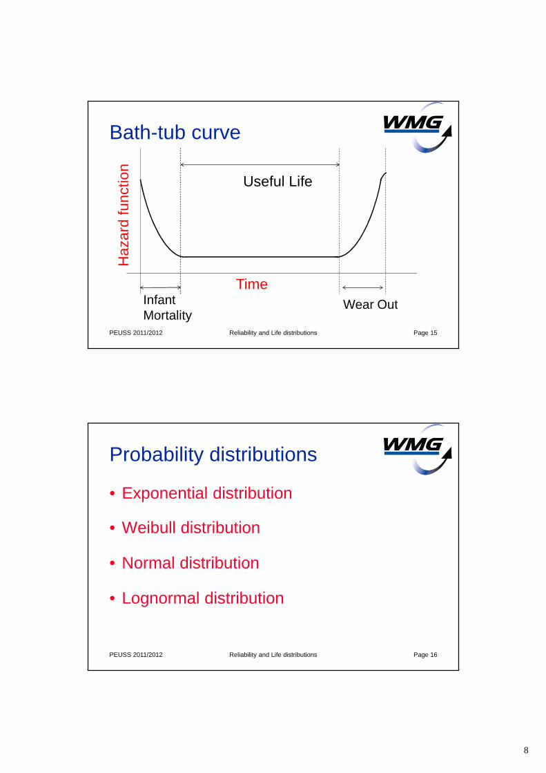
Bath-tub curve

Useful Life

InfantMortality

Wear Out

Ha

za

rdfu

nctio

n

Time


Probability distributions

• Exponential distribution

• Weibull distribution

• Normal distribution

• Lognormal distribution

9


Exponential distribution

• Simplest of all life models

• One parameter,

• PDF, f(t) = e- t

• CDF, F(t) = 1- e- t and R(t) = e- t

• Hazard function, h(t) = i.e. constant

• MTBF = 1/ and failure rate =

• 1/ is the 63rd percentile i.e. time at which 63%of population will have failed


Exponential distribution

0 10 20 30 40 50

0.150

0.155

0.160

Hazard Function

Rate0 10 20 30 40 50

0.0

0.5

1.0

Survival Function

Pro

babili

ty

10


Failure rate - example

• 10 components of a particular type in each PCB

• 5 PCBS in each unit

• 200 units in the field

• Total operating time to date for all units is 10,000 hours

• There have been 30 confirmed failures of this component

• The failure rate is given by:– 30/5*200*10*10,000 = 0.000003 = 3 fpmh (failures per million hours)

• The MTTF is 1/0.000003 = 333,333


Example

• 100 units in the field

• Total operating hours is 30,000

• Number of confirmed failures is 60

• MTBF = 30,000*100/60 = 50,000

• Removal rate includes all units removedregardless of whether they have failed

• Use 200 removals

• MTBR = 15000

11


Weibull distribution

• Most useful lifetime in reliability analysis

• 2 parameter Weibull

– Shape parameter -

– Scale parameter -

• When < 1 decreasing hazard function

• When > 1 increasing hazard function

• When =1 constant hazard function

• is the characteristic life, 63rd percentile



t

t

t

etRliability

etFCDF

ettfPDF

)(:Re

1)(:

)(: 1

12



• h(t) = t-1

• When =1, h(t)= 1/ = therefore =1/

• When >3.5 the distribution approximates to anormal distribution

Three parameter Weibull

• A three parameter distribution can be used iffailures do not start at t=0, but after a finitetime . The parameter, is called the failure-free time or location parameter

PEUSS 2011/2012 Reliability and Life distributions 24

)(

1)(

t

etF

13


Bath-tub curve and the Weibull

Useful Life

InfantMortality

Wear Out

Ha

za

rdfu

nctio

n

Time

<1=1

>1


Normal Distribution

• Not used as often in reliability work

– Can represent severe wear-out mechanism

– Rapidly Increasing hazard function

• e.g.’s, filament bulbs, IC wire bonds

• Location parameter, m , is the mean

• Scale parameter, , is the standard deviation

• Lognormal more versatile, always positive

14


Fitting parametric distributions


Fitting parametric distributions

• Censoring

• Repaired and non repaired

• Probability plotting

• Hazard plotting

15


Censoring structures

• Complete data

• Single censored– Units started together and data analysed before all units have

failed

– Right, interval and left

• Time censored– Censoring time is fixed

• Failure censored– Number of failures is fixed

• Multiply censored– Different running times intermixed with failure times – field data


Complete Data

16


Right Censored data


Interval Censored

17


Left censored


Repaired and non-repaired data

• Non-repaired data when only one failure canoccur and interested in time to failure

• Repaired data when interested in the pattern oftimes between failures

18


Probability plotting


Areas to be covered

• Introduction to probability plotting

• Assumptions

• How to do a Weibull plot

• Estimating the parameters

• Testing assumptions

• Examples

19


What is probability plotting?

• Graphical estimation method

• Based on cumulative distribution function CDF or F(t)

• Probability papers for parametric distributions, e.g.Weibull

• Axis is transformed so that the true CDF plots as astraight line

• If plotted data fits a straight line then the data fits theappropriate distribution

• Parameter estimation


Assumptions

• Data must be independently identicallydistributed (iid)– No causal relationship between data items

– No trend in the time between failures

– All having the same distribution

• Non-repaired items

• Repaired items with no trend in the timebetween failures

• Time to first failure of repaired items

20


Example of test for trend

• Machine H fails at the following running times(hours):

– 15, 42, 74, 117, 168, 233, and 410

• Machine S fails at the following running times(hours):

– 177, 242, 293, 336, 368, 395, and 410


Trend Analysis

machine H running times to failure

0

12

3

4

56

7

8

0 100 200 300 400 500

machine time to failure

ord

er

nu

mb

er

machine S running times to failure

0

12

3

4

56

7

8

0 100 200 300 400 500

machine time to failure

ord

er

nu

mb

er

This system is getting better withtime, the failure times are gettingfurther and further apart

This system is getting worse with time,the failure times are getting closer andcloser together.

In neither case can Weibull analysis be used as there istrend in the data.

21


Making a Weibull plot


Rank the data

• Probability graph papers are based on plots ofthe variable against cumulative probability

• For n< 50 the cumulative percentage probabilityis estimated using median ranks tables

• For n< 100 use benard’s approximation for themedian rank ri

ri = i - 0.3

n+0.4

Where i is the ith order value and n is the sample size

22


Example

Failure number (i) Ranked hrs at failure (ti) Median Rank from tables

Cumulative % Failed at ti - F(t)

1 300 6.7

2 410 16.2

3 500 25.9

4 600 35.5

5 660 45.2

6 750 54.8

7 825 64.5

8 900 74.1

9 1050 83.8

10 1200 93.3


• Plot times on x-axis• Plot CDF on y-axis• Fit line through the data• Draw perpendicular line from

estimation point to thefitted line.

• Read off the estimate of β• η is the value given on

from the intersection line

23


Interpreting the plot

• If the data produced a straight line then:– The data can be modelled by the Weibull distribution.

• If β<1 then data shows a decreasing hazard function– e.g. Infant mortality, weak components, low quality

• If β=1 then data shows a constant hazard function– e.g. useful life of product

• If β>1 then data shows a increasing hazard function– e.g. wear-out, product reaching end of life

• η is the value in time by which 63.2% of all failures willhave occurred and is termed the characteristic life


Bath-tub curve and the Weibull

Useful Life

InfantMortality

Wear Out

Ha

za

rdfu

nctio

n

Time

<1=1

>1

24


Interpreting the plot

• If the data did not produce a straight light then:

– There may be an amount of failure-free time

• This may appear concave when viewed from the bottomright hand corner of the sheet

– There may be more than one failure mode present

• This may appear convex shape or cranked shape (alsoknown as dog-leg shape)

• In this case the data needs to separated into failuresassociated with each failure mode using expert judgementand analysed separately

Example: Poor fit due to 3 monthsoffset


Time in service (Months)

Pe

rce

nt

100.010.01.00.1

99

9080706050403020

10

532

1

0.01

Table of Statistics

Shape 1.87010

Scale 57.6561

Mean 51.1897

Weibull Plot of Time-in-Service

Censoring Column in Censoring - ML Estimates2-Parameter Weibull - 95% CI

Time in service (Months) - Threshold

Pe

rce

nt

10000.00001000.0000100.000010.00001.00000.10000.01000.00100.0001

99

9080706050403020

10

532

1

0.01

Table of Statistics

Shape 0.873095

Scale 297.337

Thres 2.9997

Weibull Plot of Time in service (Months)

Censoring Column in Censoring - ML Estimates

3-Parameter Weibull - 95% CI

The same data plotted with a three-Parameter Weibull distribution shows a goodfit with 3 months offset (location – 2.99 months)

25

Example of two failure modes


Time to failure ( hours)

We

ibu

llC

DF

Mode 2 Beta= 11.9

Mode 1 Beta= 0.75

Adjusted rank for censored data


Rank Time StatusReverse

rank Adjusted rankMedian

rank1 10 Suspension 8 Suspended...

2 30 Failure 7 [7 X 0 +(8+1)]/ (7+1) = 1,125 9,8 %3 45 Suspension 6 Suspended…

4 49 Failure 5 [5 X 1,125 +(8+1)]/ (5+1) = 2,438 25,5 %5 82 Failure 4 [4 X 2,438 +(8+1)]/ (4+1) = 3,750 41,1 %6 90 Failure 3 [3 X 3,750 +(8+1)]/ (3+1) = 5,063 56,7 %7 96 Failure 2 [2 X 5,063 +(8+1)]/ (2+1) = 6,375 72,3 %8 100 Suspension 1 Suspended...

26


Weibull Analysis usingsoftware tools• Number of software packages that can do Weibull

plotting (and other distributions), these include:

– Minitab

– Relex

– WinSMITH

– Reliasoft

• Concentrate on getting good quality data, correctassumptions and correct interpretation from thesoftware


Hazard Plotting

27


Contents

• Assumptions

• Fitting parametric distributions

• Estimating parameters

• Using results for decision making


Assumptions

• Non-repaired items

• Repaired items with no trend in the timebetween failures

• Time to first failure of repaired items

• Individual failure modes from non-repaired items

• Can deal with censored datain particular multiply censored data

28


Hazard Plotting

• Cumulative hazard function

• Relationship allows derivation of cumulativehazard plotting paper

t

0h(t) dtH(t)=

t

0f(t) /1-F(t) dtH(t)=

-ln[1-F(t)]H(t)=


Weibull Hazard Plotting

• h(t) = t-1 and H(t) = t

• If H is the cumulative hazard value then

Log t = 1 log H + log

• Weibull hazard paper is log-log paper

• The slope is 1/ and when H=1, t=

( )

29


Hazard plotting procedure

• Tabulate times in order and rank

• Reverse rank

• For each failure, calculate the hazard interval

– hi = 1/ no of items remaining after previousfailure/censoring (i.e. 1/reverse rank)

• For each failure, calculate the cumulative hazardfunction

– H = h1 +h2 + ………. +

• Plot the cumulative hazard against life value

Hn


Example 1 – vehicle shockabsorbers

Distance (km)6700 F 17520 F6950 175407820 178908790 184509120 F 189609660 189809820 1941011310 20100 F11690 2010011850 2015011880 2032012140 20900 F12200 F 22700 F12870 2349013150 F 26510 F13330 2741013470 27490 F14040 2789014300 F 28100

Distance to failure forShock absorbersF denotes failure

30


Example 1 – vehicle shockabsorbers

Rank Reverserank

Distance(km)

Hazard(1/rank)

Cumulativehazard

1 38 6700 F 1/38 0.02632 37 69503 36 78204 35 87905 34 9120 F 1/34 0.05576 33 96607 32 98208 31 113109 30 1169010 29 1185011 28 1188012 27 1214013 26 12200 F 1/26 0.094214 25 1287015 24 13150 F 1/24 0.135916 23 1333017 22 1347018 21 1404019 20 14300 F 1/20 0.1859

20 19 17520 F 1/19 0.238521 18 1754022 17 1789023 16 1845024 15 1896025 14 1898026 13 1941027 12 20100 F 1/12 0.321828 11 2010029 10 2015030 9 2032031 8 20900 F 1/8 0.446832 7 22700 F 1/7 0.589633 6 2349034 5 26510 F 1/5 0.789635 4 2741036 3 27490 F 1/3 1.122937 2 2789038 1 28100


Example 1

• Plot the data on log 2 cycle paper x log 2 cyclepaper

• Estimate Weibull shape parameter

• Estimate Weibull scale parameter

• Interpret results

31


Example 1

Cumulative hazard plot for shock absorbers on linear

paper

0

5000

10000

15000

20000

25000

30000

0 0.2 0.4 0.6 0.8 1 1.2

Cumulative hazard

dis

tan

ce


Example 1

= 2.6= 28500kmR2 = 0.98

Log cumulative hazard for shock absorbers

1000

10000

100000

0.01 0.1 1 10

log hazard

log

dis

tan

ce

32


Survival plot for vehicle shock absorbers with

Beta =2.6 and Eta=29000km

0

0.2

0.4

0.6

0.8

1

1.2

0 5000 10000 15000 20000 25000 30000 35000 40000

kilometers

Pro

bab

ilit

yo

fsu

rviv

al

Example 1Since looking at one known failure mode use the estimatedparameters to fit to the distribution


Example 2:Hazard plot onlinear paper

Cumulative hazard plot for O ring failures

0

500

1000

1500

2000

0 1 2 3 4 5 6

cumulative hazard

ho

urs

33


Example 2: Hazard plot on logpaper

log cumulative hazard for O ring failures

1

10

100

1000

10000

0.01 0.1 1 10

log cumulative hazard

log

ho

urs

= 1.01= 360hrsR2 = 0.98


Example 2: Interpretation ofresults

• = 1.01 is approximately an exponentialdistribution and constant failure rate

• = 360 hrs = 1/ = Mean Time to Failure

• Calculating the MTTF from the data gives:

– Total hours/number of failures

– 26839/73 = 367 hrs

34


Example 2: Survival function

R(t) - Survival Function for O ring failures

0

0.2

0.4

0.6

0.8

1

1.2

0 500 1000 1500 2000

Hours to failure

Pro

bab

ilit

yo

fsu

rviv

al


Example 2: Failure Distribution

F(t) for O ring failures

0

0.2

0.4

0.6

0.8

1

1.2

0 500 1000 1500 2000

Hours to failure

Pro

bab

ilit

yo

ffa

ilu

re

35


Example 3 : pumps

• Two dominant failuremodes

– Impeller failure (I)

– Motor failure (m)

pump no age at failure failure mode

1 1180 m

2 6320 m

3 1030 i

4 120 m

5 2800 i

6 970 i

7 2150 i

8 700 m

9 640 i

10 1600 i

11 520 m

12 1090 i


Example 3: ignoring failuremodes

log cumulative hazard for all failures

1

10

100

1000

10000

0.01 0.1 1 10

cum hazard

ag

e

36


Example 3: impeller failure

log cumulative hazard plot for impeller failures

1

10

100

1000

10000

0.1 1 10

cumulative hazard

ag

ea

tfa

ilu

re

= 1.95= 1900hrsR2 = 0.93


Example 3: motor failure

log cumulative hazard plot for motor failures

1

10

100

1000

10000

0.01 0.1 1 10

cumulative hazard

ag

ea

tfa

ilu

re

= 0.76= 3647hrsR2 = 0.978

37


Advantages of Cum HazardPlotting

• It is much easier to calculate plotting positionsfor multiply censored data using cum hazardplotting techniques.

• Linear graph paper can be used for exponentialdata and log-log paper can be used for Weibulldata.


Disadvantages of CumHazard Plotting• It is less intuitively clear just what is being plotted.

– Cum percent failed (i.e., probability plots) is meaningful andthe resulting straight-line fit can be used to read off timeswhen desired percents of the population will have failed.

– Percent cumulative hazard increases beyond 100% and isharder to interpret.

• Normal cum hazard plotting techniques require exacttimes of failure and running times.

• With computer software for probability plotting, themain advantage of cum hazard plotting goes away

38


Summary

• Important lifetime distributions

– Failure distribution (CDF), Survival function R(t) andthe hazard function h(t)

• Some parametric distributions

– Exponential, Weibull and Normal

• Weibull probability plotting

• Distribution fitting using hazard plottingtechniques

an introduction to reliability and life distributions · pdf filean introduction to...

Documents