An introduction to relativistic An introduction to relativistic hydrodynamics and magnetohydrodynamics and magneto--hydrodynamicshydrodynamics

José A. FontJosé A. FontDepartamento de Astronomía y Astrofísica Departamento de Astronomía y Astrofísica

Universidad de Valencia (Spain)Universidad de Valencia (Spain)

Talk given at the Aristotle University of Thessaloniki, Dec. 7thTalk given at the Aristotle University of Thessaloniki, Dec. 7th 20052005

OutlineOutline of the of the talktalk

• Introduction & MotivationIntroduction & Motivation

•• General relativistic hydrodynamics equations (3+1)General relativistic hydrodynamics equations (3+1)

•• General relativistic (ideal) magnetoGeneral relativistic (ideal) magneto--hydrodynamics equationshydrodynamics equations

•• Numerical solution (hyperbolic systems of conservation laws)Numerical solution (hyperbolic systems of conservation laws)

••Applications in relativistic astrophysicsApplications in relativistic astrophysics

Further informationFurther information::

J.A. Font,J.A. Font, “Numerical hydrodynamics in general relativity”,“Numerical hydrodynamics in general relativity”, Living Reviews in Relativity Living Reviews in Relativity (2003) ((2003) (www.livingreviews.orgwww.livingreviews.org))

L. Antón, O. Zanotti, J.A. Miralles, J.M. Martí, J.M. Ibáñez, J.L. Antón, O. Zanotti, J.A. Miralles, J.M. Martí, J.M. Ibáñez, J.A. Font, J.A. Pons,A. Font, J.A. Pons,“Numerical 3+1 general relativistic magnetohydrodynamics: a loca“Numerical 3+1 general relativistic magnetohydrodynamics: a local characteristic approach”l characteristic approach”(ApJ in press; astro(ApJ in press; astro--ph/0506063)ph/0506063)

Part 1Part 1Introduction & MotivationIntroduction & Motivation

Introduction & MotivationIntroduction & MotivationThe natural domain of applicability ofThe natural domain of applicability of general relativistic hydrodynamics (GRHD) and general relativistic hydrodynamics (GRHD) and magnetohydrodynamics (GRMHD)magnetohydrodynamics (GRMHD) is in the field ofis in the field of relativistic astrophysics.relativistic astrophysics.General relativityGeneral relativity andand relativistic (magnetorelativistic (magneto--)hydrodynamics)hydrodynamics play a major role in the play a major role in the description ofdescription of gravitational collapsegravitational collapse leading to the formation ofleading to the formation of compact objects (neutron compact objects (neutron stars and black holes): stars and black holes):

• Stellar coreStellar core--collapse supernovae collapse supernovae (Type II/Ib/Ic)(Type II/Ib/Ic)

•• Black hole formation (and accretion)Black hole formation (and accretion)

•• Coalescing compact binaries Coalescing compact binaries (NS/NS, BH/NS, BH/BH)(NS/NS, BH/NS, BH/BH)

•• gammagamma--ray bursts ray bursts

•• jet formation (black hole plus thick disc systems)jet formation (black hole plus thick disc systems)

TimeTime--dependent evolutionsdependent evolutions of fluid flow of fluid flow coupledcoupled to the spacetime geometry (Einstein’s to the spacetime geometry (Einstein’s equations) only possible through accurate, largeequations) only possible through accurate, large--scale scale numerical simulations.numerical simulations.

Some scenarios can be described in the Some scenarios can be described in the testtest--fluid approximationfluid approximation: GRHD/GRMHD : GRHD/GRMHD computations in curved backgrounds (highly mature nowadays, partcomputations in curved backgrounds (highly mature nowadays, particularly GRHD case).icularly GRHD case).

The GRHD/GRMHD equations constitute nonlinear hyperbolic systemsThe GRHD/GRMHD equations constitute nonlinear hyperbolic systems. . Solid mathematical foundations and accurate numerical methodologSolid mathematical foundations and accurate numerical methodology imported from CFD. A y imported from CFD. A “preferred” choice: “preferred” choice: highhigh--resolution shockresolution shock--capturing schemes written in conservation form.capturing schemes written in conservation form.

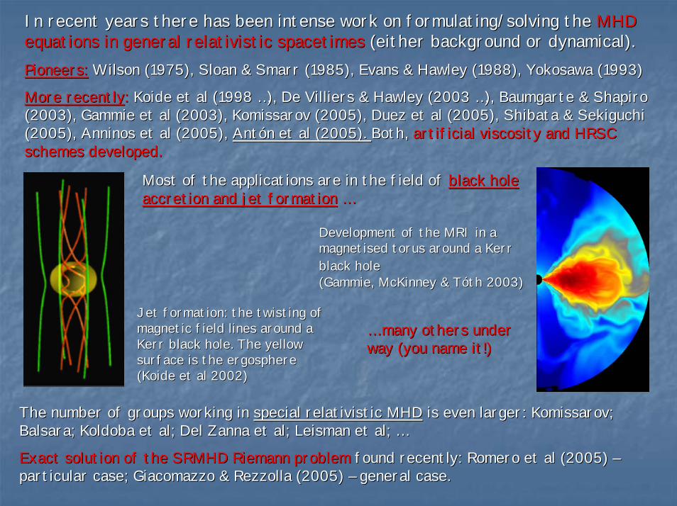
In recent years there has been intense work on formulating/solviIn recent years there has been intense work on formulating/solving the ng the MHD MHD equations in general relativistic spacetimesequations in general relativistic spacetimes (either background or dynamical).(either background or dynamical).Pioneers:Pioneers: Wilson (1975), Sloan & Smarr (1985), Evans & Hawley (1988), YokWilson (1975), Sloan & Smarr (1985), Evans & Hawley (1988), Yokosawa (1993)osawa (1993)

More recentlyMore recently:: Koide et al (1998 …), De Villiers & Hawley (2003 …), Baumgarte Koide et al (1998 …), De Villiers & Hawley (2003 …), Baumgarte & Shapiro & Shapiro (2003), Gammie et al (2003), Komissarov (2005), Duez et al (2005(2003), Gammie et al (2003), Komissarov (2005), Duez et al (2005), Shibata & Sekiguchi ), Shibata & Sekiguchi (2005), Anninos et al (2005), (2005), Anninos et al (2005), Antón et al (2005). Antón et al (2005). Both, Both, artificial viscosity and HRSC artificial viscosity and HRSC schemes developed.schemes developed.

Most of the applications are in the field of Most of the applications are in the field of black hole black hole accretion and jet formationaccretion and jet formation ……

Development of the MRI in a Development of the MRI in a magnetised torus around a Kerr magnetised torus around a Kerr black holeblack hole(Gammie, McKinney & Tóth 2003)(Gammie, McKinney & Tóth 2003)

Jet formation: the twisting of Jet formation: the twisting of magnetic field lines around a magnetic field lines around a Kerr black hole. The yellow Kerr black hole. The yellow surface is the ergosphere surface is the ergosphere (Koide et al 2002) (Koide et al 2002)

…… many others under many others under way (you name it!)way (you name it!)

The number of groups working in The number of groups working in special relativistic MHDspecial relativistic MHD is even larger: Komissarov; is even larger: Komissarov; Balsara; Koldoba et al; Del Zanna et al; Leisman et al; … Balsara; Koldoba et al; Del Zanna et al; Leisman et al; …

Exact solution of the SRMHD Riemann problemExact solution of the SRMHD Riemann problem found recently: Romero et al (2005) found recently: Romero et al (2005) ––particular case; Giacomazzo & Rezzolla (2005) particular case; Giacomazzo & Rezzolla (2005) –– general case.general case.

Part 2Part 2General relativistic hydrodynamics equationsGeneral relativistic hydrodynamics equations

A brief reminder: Classical (Newtonian) hydrodynamicsA brief reminder: Classical (Newtonian) hydrodynamics

Mass conservation (continuity equation)Mass conservation (continuity equation)

Let Let VVtt be a volume which moves with the fluid; its mass is given bybe a volume which moves with the fluid; its mass is given by

From the From the principle of conservation of massprinciple of conservation of mass enclosed within that volumeenclosed within that volume

( ) ( )dVrtVmtVt ,∫= ρ

( ) ( ) 0 , == ∫ dVrtdtdVm

dtd

tVt ρ ( ) 0 =⋅∇+∂∂

⇒ vt

ρρ

CorolaryCorolary:: the variation of the mass enclosed in a fixed volume the variation of the mass enclosed in a fixed volume VVis equal to the flux of mass across the surface at the is equal to the flux of mass across the surface at the boundary of the volume.

∫ ∫∂ Σ⋅=∂∂

−V V

dvdVt

ρρ boundary of the volume.

Momentum balance (Euler’s equation)Momentum balance (Euler’s equation)

““the variation of momentum of a given portion of fluid is equal tthe variation of momentum of a given portion of fluid is equal to the net force o the net force (stresses plus external forces) exerted on it(stresses plus external forces) exerted on it” (” (Newton’s 2nd lawNewton’s 2nd law):):

[ ]∫ ∫ ∫∫ ∂∇−=+Σ−=

t t tt V V VVdVpGdVGdpdVv

dtd ρ

pGapGDt

vD∇−=⇔∇−= ρρ

Energy conservationEnergy conservation

Let E be the Let E be the total energytotal energy of the fluid, sum of its of the fluid, sum of its kinetic energykinetic energy and its and its internal energyinternal energy::

∫ ∫+=+=t tV V

dVdVvEEE 21 2

intK ρερ

Principle of energy conservationPrinciple of energy conservation: “: “the variation in time of the total energy of a portion the variation in time of the total energy of a portion of fluid is equal to the work done per unit time over the systemof fluid is equal to the work done per unit time over the system by the stresses by the stresses (internal forces) and the external forces(internal forces) and the external forces”.”.

∫ ∫ ∫∂⋅+Σ⋅−=⎟

⎠⎞

⎜⎝⎛ +=

t t tV V VdVvGdvpdVv

dtd

dtdE

21 2 ρερ vgvpvv

t⋅=⎥

⎦

⎤⎢⎣

⎡⎟⎠⎞

⎜⎝⎛ ++⋅∇+⎟

⎠⎞

⎜⎝⎛ +

∂∂ ρρερρερ 22

21

21

ρπGg 4 , =∆ΦΦ∇−=is a conservative external force field (e.g. gravitational fieldis a conservative external force field (e.g. gravitational field):):g

The above equations are a The above equations are a nonlinear nonlinear hyperbolic system of conservation lawshyperbolic system of conservation laws::

( ) ( )usxuf

tu

i

i

=∂

∂+

∂∂

( )( )( )⎟⎠⎞

⎜⎝⎛

∂Φ∂

−∂Φ∂

−=

++=

=

ii

j

iijjiii

j

xv

xs

vpepvvvf

evu

ρρ

δρρ

ρρ

,,0

,,

,,

Hyperbolic equations have finite propagation Hyperbolic equations have finite propagation speedspeed: maximum speed of information given by : maximum speed of information given by the largest characteristic curves of the system. the largest characteristic curves of the system.

The The range of influencerange of influence of the solution is of the solution is bounded by the bounded by the eigenvalues of the Jacobian eigenvalues of the Jacobian matrix of the system.

state vectorstate vectormatrix of the system.

flux vectorflux vector

sii

i

cvvufA ±==⇒∂∂

= ±λλ ,0source vectorsource vector

General Relativistic Hydrodynamics equationsGeneral Relativistic Hydrodynamics equationsThe general relativistic hydrodynamics equations are obtained frThe general relativistic hydrodynamics equations are obtained from the om the local conservation local conservation laws of the stresslaws of the stress--energy tensorenergy tensor, , TTµνµν (the Bianchi identities), (the Bianchi identities), and the matter current and the matter current densitydensity JJµµ (the continuity equation):(the continuity equation):

0=∇ µνµT 0=∇ µ

µ J Equations of motionEquations of motion

( ) ( ) µννµµνµννµµν ησζερ uquqhpuuT ++−Θ−++≡ 21

As usual As usual ∇∇µµ stands for the covariant derivative associated with the four dimstands for the covariant derivative associated with the four dimensional ensional spacetime metric spacetime metric ggµνµν. The density current is given by . The density current is given by JJµµ==ρρuuµµ, , uuµµ representing the fluid 4representing the fluid 4--velocity and velocity and ρρ the restthe rest--mass density in a locally inertial reference frame.mass density in a locally inertial reference frame.

The stressThe stress--energy tensor for a energy tensor for a nonnon--perfect fluidperfect fluid is defined as: is defined as:

where where εε is the restis the rest--frame specific internal energy density of the fluid, frame specific internal energy density of the fluid, pp is the pressure, is the pressure, and and hhµνµν is the spatial projection tensor, is the spatial projection tensor, hhµνµν==uuµµuuνν++ggµνµν. In addition, . In addition, ζζ and and ηη are the shear are the shear and bulk viscosity coefficients. The expansion, and bulk viscosity coefficients. The expansion, ΘΘ, describing the divergence or , describing the divergence or convergence of the fluid world lines is defined as convergence of the fluid world lines is defined as ΘΘ==∇∇µµuuνν. The symmetric, trace. The symmetric, trace--free, and free, and spatial shear tensor spatial shear tensor σσµνµν is defined by:is defined by:

Finally Finally qqµµ is the energy flux vector. is the energy flux vector.

( ) µναµνα

ανµα

µνσ hhuhu Θ−∇+∇=31

21

In the following we will In the following we will neglect nonneglect non--adiabatic effectsadiabatic effects, such as viscosity or heat transfer, , such as viscosity or heat transfer, assuming the assuming the stressstress--energy tensorenergy tensor to be that of a to be that of a perfect fluidperfect fluid::

where we have introduced the relativistic specific enthalpy, where we have introduced the relativistic specific enthalpy, hh, defined as:

µννµµν ρ pguhuT +≡, defined as:

ρε ph ++=1

Introducing an explicit Introducing an explicit coordinate chartcoordinate chart the previous conservation equations read:the previous conservation equations read:

µλνµλ

µνµ

µµ ρ

TgTgx

ugx

Γ−=−∂∂

=−∂∂

)(

0)(

where the scalar where the scalar xx00 represents a foliation of the spacetime with hypersurfaces represents a foliation of the spacetime with hypersurfaces (coordinatised by (coordinatised by xxii). Additionally, is the volume element associated with t). Additionally, is the volume element associated with the 4he 4--metric metric ggµνµν, with , with gg=det(=det(ggµνµν), and are the 4), and are the 4--dimensional Christoffel symbols.dimensional Christoffel symbols.

The system formed by the equations of motion and the continuity The system formed by the equations of motion and the continuity equation must be equation must be supplemented with an supplemented with an equation of stateequation of state (EOS)(EOS) relating the pressure to some fundamental relating the pressure to some fundamental thermodynamical quantities, e.g.thermodynamical quantities, e.g.

g−νµλΓ

( )ερ ,pp =•• Ideal fluid EOS:Ideal fluid EOS:

•• Polytropic EOS:Polytropic EOS:

( )ρε1−Γ=p

( )np 11 , +=Γ= Γκρ

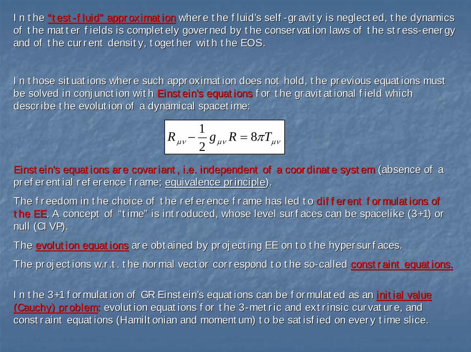
In the In the “test“test--fluid” approximationfluid” approximation where the fluid’s selfwhere the fluid’s self--gravity is neglected, the dynamics gravity is neglected, the dynamics of the matter fields is completely governed by the conservation of the matter fields is completely governed by the conservation laws of the stresslaws of the stress--energy energy and of the current density, together with the EOS.and of the current density, together with the EOS.

In those situations where such approximation does not hold, the In those situations where such approximation does not hold, the previous equations must previous equations must be solved in conjunction with be solved in conjunction with Einstein’s equationsEinstein’s equations for the gravitational field which for the gravitational field which describe the evolution of a dynamical spacetime:describe the evolution of a dynamical spacetime:

µνµνµν πTRgR 821

=−

Einstein’s equations Einstein’s equations are covariant, i.e. independent of a coordinate system are covariant, i.e. independent of a coordinate system (absence of a (absence of a preferential reference frame; preferential reference frame; equivalence principleequivalence principle). ).

The freedom in the choice of the reference frame has led to The freedom in the choice of the reference frame has led to different formulations of different formulations of the EEthe EE. A concept of . A concept of ““timetime”” is introduced, whose level surfaces can be spacelike (3+1) or is introduced, whose level surfaces can be spacelike (3+1) or null (CIVP). null (CIVP).

The The evolution equationsevolution equations are obtained by projecting EE on to the hypersurfaces.are obtained by projecting EE on to the hypersurfaces.

The projections w.r.t. the normal vector correspond to the soThe projections w.r.t. the normal vector correspond to the so--called called constraint equations.constraint equations.

In the 3+1 formulation of GR Einstein’s equations can be formulaIn the 3+1 formulation of GR Einstein’s equations can be formulated as an ted as an initial value initial value (Cauchy) problem(Cauchy) problem:: evolution equations for the 3evolution equations for the 3--metric and extrinsic curvature, and metric and extrinsic curvature, and constraint equations (Hamiltonian and momentum) to be satisfied constraint equations (Hamiltonian and momentum) to be satisfied on every time slice.on every time slice.

Einstein’s equations in the 3+1 formulationEinstein’s equations in the 3+1 formulation ( )ijij K,γ

The most widely used approach to formulate and solve Einstein’s The most widely used approach to formulate and solve Einstein’s equations in Numerical equations in Numerical Relativity is the soRelativity is the so--called called Cauchy or 3+1 formulationCauchy or 3+1 formulation. .

Lichnerowicz (1944); ChoquetLichnerowicz (1944); Choquet--Bruhat (1962); Arnowitt, Deser & Misner (1962); York (1979)Bruhat (1962); Arnowitt, Deser & Misner (1962); York (1979)

Spacetime is foliated with a set of nonSpacetime is foliated with a set of non--intersecting spacelike hypersurfaces intersecting spacelike hypersurfaces ΣΣ. Within . Within each surface distances are measured with the spatial each surface distances are measured with the spatial 33--metricmetric γγijij.. The The extrinsic curvature extrinsic curvature tensortensor KKij ij is also introduced. This tensor describes how the spacelike hipis also introduced. This tensor describes how the spacelike hipersurfaces are ersurfaces are ““embeddedembedded”” in spacetime. in spacetime.

There are There are two kinematical variablestwo kinematical variables which describe the evolution between each which describe the evolution between each hypersurface: the hypersurface: the lapse functionlapse function αα which describes the rate of proper time along a which describes the rate of proper time along a timelike unit vector normal to the hypersurface, and the shift vtimelike unit vector normal to the hypersurface, and the shift vector ector ββii, spacelike vector , spacelike vector which describes the movement of coordinates within the hypersurfwhich describes the movement of coordinates within the hypersurface.ace.

jdxidxijdtidxidtiids γβββα ++−−= 2)( 222

( )0,0,0, ,,1

ααβ

α

βα

µµ −=⎟⎟

⎠

⎞⎜⎜⎝

⎛−=

∂+=∂

nn

ni

ii

t

Metric:Metric:

lklj

kiij nK ∇−≡ γγ

(Numerical) General Relativity: (Numerical) General Relativity: Which portion of spacetime shall we foliate?Which portion of spacetime shall we foliate?

3+1 (Cauchy) formulation3+1 (Cauchy) formulationLichnerowicz (1944); ChoquetLichnerowicz (1944); Choquet--Bruhat (1962); Arnowitt, Deser Bruhat (1962); Arnowitt, Deser & Misner (1962); York (1979)& Misner (1962); York (1979)

Standard choice for most Numerical Relativity groups.Standard choice for most Numerical Relativity groups.

Spatial hypersurfaces have a Spatial hypersurfaces have a finitefinite extension. extension.

( )

( ) 08

016

82

2

0022

=−−∇

=−−+

−∇+∇+∇+−++∇−∇=∂

∇+∇+−=∂

jijiji

ijij

ijm

ijmm

jimijmmm

jimijijjiijt

ijjiijijt

SKK

TKKKR

TKKKKKKKRK

K

πγ

πα

πβββαα

ββαγ (original formulation of the 3+1 equations)(original formulation of the 3+1 equations)

Reformulating these equations to achieve numerical Reformulating these equations to achieve numerical stability is one of the arts of numerical relativity.stability is one of the arts of numerical relativity.

Conformal formulation: Conformal formulation: Spatial hypersurfaces have Spatial hypersurfaces have infiniteinfinite extension extension (Friedrich et al).(Friedrich et al).

Characteristic formulation Characteristic formulation (Winicour (Winicour et al).et al).

Hypersuperfaces are light cones Hypersuperfaces are light cones (incoming/outgoing) with (incoming/outgoing) with infiniteinfiniteextension.extension.

( )

ijijij

mijm

mjimijm

m

mjimijijjiijt

ijjiijijt

SS

KKK

KKKKRK

K

παργγπα

βββ

αα

ββαγ

4218

2

2

−⎟⎠⎞

⎜⎝⎛ −−

∇+∇+∇+

−++∇−∇=∂

∇+∇+−=∂j

jijij

j

ijij

SKK

KKKR

πγ

πρ

8

162

=∇−∇

=−+

Constraint equations:Constraint equations:Evolution equations:Evolution equations:

Definitions:Definitions: Cauchy problem (IVP) for the 3+1 Cauchy problem (IVP) for the 3+1 formulation of Einstein’s equations: formulation of Einstein’s equations:

• Prescribe Prescribe γγijij, , KKijij at at tt=0 subject to =0 subject to the constraint equations. the constraint equations.

•• Specify coordinates via Specify coordinates via αα and and ββ

•• Evolve data using evolution equations Evolve data using evolution equations for for γγijij, , KKijij..

Bianchi identitiesBianchi identities guarantee that if guarantee that if the constraints are satisfied at t=0, the constraints are satisfied at t=0, theythey’’ll be satisfied at t>0; that is, the ll be satisfied at t>0; that is, the evolution equations satisfy the evolution equations satisfy the constraint equations. constraint equations.

( )

PvvhWS

PvvhWTS

vhWnTS

PhWnnT

KK

RR

R

ii

ijjijiij

iii

ijij

ijij

jknnkjnjkini

jk

min

njm

mij

nmn

ninj

nijnij

i

3

21

2

2

2

2

+=

+=⊥≡⊥

=⊥−≡

−=≡

=

=

∂−∂+∂=Γ

ΓΓ−ΓΓ+Γ∂−Γ∂=

∇

ρ

γρ

ρ

ρρ

γ

γ

γγγγ

µννµ

νµν

µ

νµµν

Covariant derivative w.r.t. sopatial metricCovariant derivative w.r.t. sopatial metric

Ricci tensorRicci tensor

Christoffel symbolsChristoffel symbols

Scalar curvatureScalar curvature

Trace of extrinsic curvatureTrace of extrinsic curvature

Matter termsMatter terms

3+1 GR Hydro equations 3+1 GR Hydro equations -- formulationsformulations

Different formulationsDifferent formulations exist depending on:exist depending on:

1.1. The choice of timeThe choice of time--slicingslicing: the level surfaces of : the level surfaces of can be spatial (3+1) or null (characteristic)can be spatial (3+1) or null (characteristic)

2.2. The choice of The choice of physical (primitive) variablesphysical (primitive) variables ((ρρ, , εε, u, ui i …)…)

0xµλν

µλµν

µ

µµ ρ

TgTgx

ugx

Γ−=−∂∂

=−∂∂

)(

0)(

Wilson (1972)Wilson (1972) wrote the system as a set of advection equation within the 3+1 wrote the system as a set of advection equation within the 3+1 formalism. formalism. NonNon--conservative.conservative.

Conservative formulationsConservative formulations wellwell--adapted to numerical methodology are more recent:adapted to numerical methodology are more recent:

•• Martí, Ibáñez & Miralles (1991):Martí, Ibáñez & Miralles (1991): 1+1, general EOS1+1, general EOS

•• Eulderink & Mellema (1995):Eulderink & Mellema (1995): covariant, perfect fluidcovariant, perfect fluid

•• Banyuls et al (1997):Banyuls et al (1997): 3+1, general EOS3+1, general EOS

•• Papadopoulos & Font (2000):Papadopoulos & Font (2000): covariant, general EOScovariant, general EOS

Numerically, the Numerically, the hyperbolic and conservativehyperbolic and conservative nature of the GRHD equations allows to nature of the GRHD equations allows to design a solution procedure based on the design a solution procedure based on the characteristic speeds and fields of the systemcharacteristic speeds and fields of the system, , translating to relativistic hydrodynamics existing tools of CFD.translating to relativistic hydrodynamics existing tools of CFD.

This procedure departs from earlier approachesThis procedure departs from earlier approaches, most notably in avoiding the need for , most notably in avoiding the need for artificial dissipation terms to handle discontinuous solutions aartificial dissipation terms to handle discontinuous solutions as well as implicit schemes as s well as implicit schemes as proposed by Norman & Winkler (1986).proposed by Norman & Winkler (1986).

3+1 GR Hydro equations 3+1 GR Hydro equations –– Eulerian observerEulerian observer

jdxidxijdtidxidtiids γβββα ++−−= 2)( 222

FoliateFoliate thethe spacetimespacetime withwith t=constt=constspatial spatial hypersurfaceshypersurfaces ∑∑tt

LetLet nn be the unit be the unit timeliketimelike44--vectorvector orthogonalorthogonal to to ∑∑tt such such thatthat

)(1n ii

t ∂−∂= βα

Eulerian observer:Eulerian observer: at rest in a given hypersurface, moves from at rest in a given hypersurface, moves from ∑∑ttto to ∑∑t+t+∆∆tt along the normal to the slice:along the normal to the slice:

unnv⋅∂⋅

−≡ i ⎟⎟⎠

⎞⎜⎜⎝

⎛+= i

t

ii

uuv β

α1

Definitions:Definitions: u :u : fluid’s 4fluid’s 4--velocity, velocity, p p :: isotropic pressure, isotropic pressure, ρρ :: restrest--mass mass density density εε : specific internal energy density, : specific internal energy density, e=e=ρρ(( 1+1+εε) ) :: energy densityenergy density

The extension of modern HRSC schemes from classical fluid dynamiThe extension of modern HRSC schemes from classical fluid dynamics to relativistic cs to relativistic hydrodynamics was accomplished in hydrodynamics was accomplished in three stepsthree steps::

1.1. Casting the GRHD equations as a system of conservation laws.Casting the GRHD equations as a system of conservation laws.

2.2. Identifying the suitable vector of unknowns.Identifying the suitable vector of unknowns.

3.3. Building up an approximate Riemann solver (or highBuilding up an approximate Riemann solver (or high--order symmetric scheme).order symmetric scheme).

Replace the Replace the “primitive“primitive variables”variables” inin terms terms of the of the ““conserved conserved variables” :variables” :

( )⎪⎩

⎪⎨

⎧

−≡

≡

≡

→=

phWE

vhWSWD

vw jji

2

2 ,,

ρ

ρ

ρ

ερ ρε ph ++≡ 1

specific enthalpyspecific enthalpy )1/(12

jjvvW −≡

Lorentz factorLorentz factor

)( )()(1 ws

xwfg

twu

g i

i

=⎟⎟⎠

⎞⎜⎜⎝

⎛

∂−∂

+∂

∂−

γ

( )DESDwu j −= ,,)(

⎟⎟⎠

⎞⎜⎜⎝

⎛+⎟⎟

⎠

⎞⎜⎜⎝

⎛−−+⎟⎟

⎠

⎞⎜⎜⎝

⎛−⎟⎟

⎠

⎞⎜⎜⎝

⎛−= i

iii

j

ii

j

iii pvvDEpvSvDwf

αβδ

αβ

αβ ,,)(

FirstFirst--order fluxorder flux--conservative hyperbolic systemconservative hyperbolic system

⎟⎟⎠

⎞⎜⎜⎝

⎛⎟⎠⎞

⎜⎝⎛ Γ−

∂∂

⎟⎟⎠

⎞⎜⎜⎝

⎛Γ−

∂

∂= 00 ln,,0)( µν

µνµ

µδ

δµνµ

νµν αα Tx

Tgxg

Tws jj

fluxesfluxes

sourcessources

Banyuls et al, ApJ, Banyuls et al, ApJ, 476476, 221 , 221 (1997)(1997)

Font et al, PRD, Font et al, PRD, 6161, 044011 , 044011 (2000)(2000)

state vectorstate vector

Recovering special relativistic and Newtonian limitsRecovering special relativistic and Newtonian limits

( )

( ) ( )⎟⎠⎞

⎜⎝⎛ Γ−

∂∂

=⎟⎟⎠

⎞⎜⎜⎝

⎛

∂−−∂

+∂

−−∂−

⎟⎟⎠

⎞⎜⎜⎝

⎛Γ−

∂

∂=⎟

⎟⎠

⎞⎜⎜⎝

⎛

∂+−∂

+∂

∂−

=⎟⎟⎠

⎞⎜⎜⎝

⎛

∂−∂

+∂

∂−

0022

22

ln1

1

01

µνµν

µµ

δδµνµ

νµν

ααρρρργ

δρργ

ρργ

Tx

Tx

vWhWgt

WphWg

gxg

Tx

pvvhWgt

vhWg

xWvg

tW

g

i

i

jj

i

ijjij

i

i General RelativityGeneral Relativity

( )

021

21

0

0

22

=∂

⎟⎠⎞

⎜⎝⎛ ++∂

+∂

⎟⎠⎞

⎜⎝⎛ +∂

=∂+∂

+∂

∂

=∂∂

+∂∂

i

i

i

ijjij

i

i

x

vpv

t

v

xpvv

tv

xv

t

ρρερρε

δρρ

ρρ NewtonNewton

( )

( ) ( ) 0

0

0

22

22

=∂−∂

+∂

−−∂

=∂

+∂+

∂∂

=∂

∂+

∂∂

i

i

i

ijjij

i

i

xvWhW

tWphW

xpvvhW

tvhW

xWv

tW

ρρρρ

δρρ

ρρ MinkowskiMinkowski

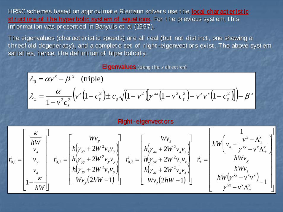
HRSC schemes based on approximate Riemann solvers use the HRSC schemes based on approximate Riemann solvers use the local characteristic local characteristic structure of the hyperbolic system of equationsstructure of the hyperbolic system of equations.. For the previous system, this For the previous system, this information was presented in Banyuls et al (1997). information was presented in Banyuls et al (1997).

The eigenvalues (characteristic speeds) are all real (but not diThe eigenvalues (characteristic speeds) are all real (but not distinct, one showing a stinct, one showing a threefold degeneracy), and a complete set of rightthreefold degeneracy), and a complete set of right--eigenvectors exist. The above system eigenvectors exist. The above system satisfies, hence, the definition of hiperbolicity.satisfies, hence, the definition of hiperbolicity.

EigenvaluesEigenvalues (along the (along the xx direction)direction)

( ) ( ) ( ) ( )[ ]( ) xs

xxs

xxss

x

s

xx

cvvcvvccvcv

v

βγαλ

βαλ

−−−−−±−−

=

−=

±22222

22

0

11111

(triple)

RightRight--eigenvectorseigenvectors

( )( )( )

( )

( )( )( )

( ) ( )⎥⎥⎥⎥⎥⎥⎥⎥

⎦

⎤

⎢⎢⎢⎢⎢⎢⎢⎢

⎣

⎡

−Λ−

−

⎟⎟⎠

⎞⎜⎜⎝

⎛Λ−

Λ−−

=

⎥⎥⎥⎥⎥⎥

⎦

⎤

⎢⎢⎢⎢⎢⎢

⎣

⎡

−+++

=

⎥⎥⎥⎥⎥⎥

⎦

⎤

⎢⎢⎢⎢⎢⎢

⎣

⎡

−+++

=

⎥⎥⎥⎥⎥⎥⎥⎥

⎦

⎤

⎢⎢⎢⎢⎢⎢⎢⎢

⎣

⎡

−

=

±

±

±

±

1

1

12222

12222

1

2

2

2

3,02

2

2

2,01,0

xxxx

xxxxz

y

xxxx

xx

x

z

zzzz

zyyz

zxxz

z

y

yzzy

yyyy

yxxy

y

z

y

x

vvvhW

hWvhWv

vvvhW

r

hWWvvvWhvvWhvvWh

Wv

r

hWWvvvWhvvWhvvWh

Wv

r

hW

vvv

hW

r

γγ

γ

γγγ

γγγ

κ

κ

( ) ( ) ( )[ ]( )222222

0

1111

1(triple)

sxxxx

ssx

s

x

cvvvvvvccvcv

v

−−−−±−−

=

=

±λ

λSpecial relativistic limit Special relativistic limit (along x(along x--direction)direction)

coupling with transversal components of the velocity coupling with transversal components of the velocity (important difference with Newtonian case)(important difference with Newtonian case)

Even in the purely 1D case:Even in the purely 1D case: ( )s

xs

xxx

cvcvvvv

±±

==⇒= ± 1 , 0,0, 0 λλ

For causal EOS the sound cone lies within the light coneFor causal EOS the sound cone lies within the light cone

Recall Newtonian (1D) case:Recall Newtonian (1D) case:

sxx cvv ±== ±λλ ,0

Part 3Part 3General relativistic (ideal) magnetoGeneral relativistic (ideal) magneto--hydrodynamics hydrodynamics

equationsequations

3+1 General Relativistic (Ideal) 3+1 General Relativistic (Ideal) MagnetohydrodynamicsMagnetohydrodynamics equations (1)equations (1)

GRMHD: Dynamics of relativistic, electrically conducting fluids GRMHD: Dynamics of relativistic, electrically conducting fluids in the presence of in the presence of magnetic fields.magnetic fields.

Ideal GRMHDIdeal GRMHD: Absence of viscosity effects and heat conduction in the limit : Absence of viscosity effects and heat conduction in the limit ofof infinite infinite conductivityconductivity (perfect conductor fluid).(perfect conductor fluid).

TheThe stressstress--energy tensorenergy tensor includes the contribution from theincludes the contribution from the perfect fluidperfect fluid and from theand from themagnetic fieldmagnetic field measured by the observer comoving with the fluid.measured by the observer comoving with the fluid.µb

νµµννµλδ

λδµννλ

µλµν

µννµµν

µνµνµν

ρ

bbbguuFFgFFT

pguhuT

TTT

−⎟⎠⎞

⎜⎝⎛ +=−≡

+≡

+≡

2EM

PF

EMPF

21

41

0

=

−=

νµν

δλµνλδµν η

uF

buF

νµµννµµν ρ bbgpuuhT −+= ∗∗

ρ

νν

2

2

2

2bhh

bpp

bbb

+=

+=

=

∗

∗

with the definitions:with the definitions:

Ideal MHD condition: Ideal MHD condition: electric fourelectric four--current current must be finite.must be finite. ( )∞→+= σσρ ν

µνµµ q uFuJ

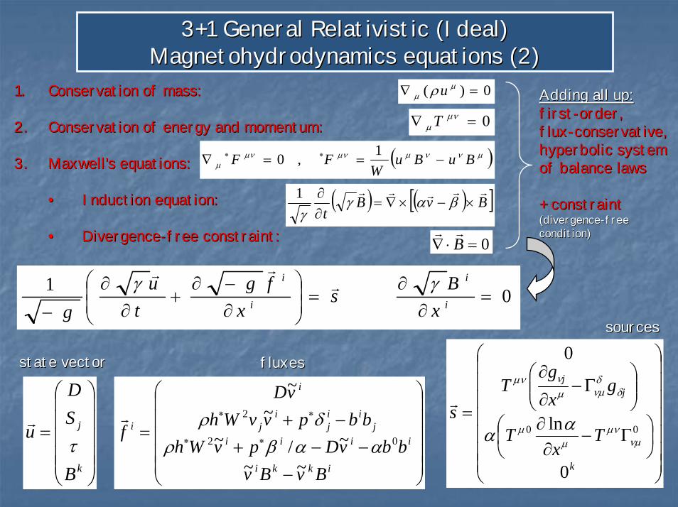
3+1 General Relativistic (Ideal) 3+1 General Relativistic (Ideal) MagnetohydrodynamicsMagnetohydrodynamics equations (2)equations (2)

1.1. Conservation of mass:Conservation of mass:

2.2. Conservation of energy and momentum: Conservation of energy and momentum:

3.3. Maxwell’s equations:Maxwell’s equations:

•• Induction equation:Induction equation:

•• DivergenceDivergence--free constraint:free constraint:

( ) ( )[ ]BvBt

×−×∇=∂∂ βαγ

γ1

0)( =∇ µµ ρu

0=∇ µνµT

( )µννµµνµνµ BuBu

WFF −==∇ ∗∗ 1 , 0

0=⋅∇ B

0 1=

∂∂

=⎟⎟⎠

⎞⎜⎜⎝

⎛

∂−∂

+∂

∂− i

i

i

i

xB

sx

fgt

ug

γγ

⎟⎟⎟⎟⎟

⎠

⎞

⎜⎜⎜⎜⎜

⎝

⎛

=

k

j

B

SD

uτ

⎟⎟⎟⎟⎟

⎠

⎞

⎜⎜⎜⎜⎜

⎝

⎛

−−−+

−+=

∗∗

∗∗

ikki

iiiij

iij

ij

i

i

BvBvbbvDpvWh

bbpvvWhvD

f

~~~/~

~~

02

2

ααβρδρ

⎟⎟⎟⎟⎟⎟⎟

⎠

⎞

⎜⎜⎜⎜⎜⎜⎜

⎝

⎛

⎟⎠⎞

⎜⎝⎛ Γ−

∂∂

⎟⎟⎠

⎞⎜⎜⎝

⎛Γ−

∂

∂

=

k

jj

Tx

T

gxg

Ts

0

ln

0

00νµ

µνµ

µ

δδνµµ

νµν

αα

Adding all up:Adding all up:firstfirst--order, order, fluxflux--conservative, conservative, hyperbolic system hyperbolic system of balance lawsof balance laws

+ constraint+ constraint(divergence(divergence--free free condition)condition)

sourcessources

state vectorstate vector fluxesfluxes

Part 4Part 4Numerical solution Numerical solution

(hyperbolic systems of conservation laws)(hyperbolic systems of conservation laws)

A standard implementation of a HRSC FD schemeA standard implementation of a HRSC FD scheme

⎟⎠⎞⎜

⎝⎛ −

∆∆

−= −++ n

jnj

nj

nj ff

xtuu 2/12/1

1 ˆˆ

⎥⎦

⎤⎢⎣

⎡∆−+= ∑

=nn

nnLiRii Rwfwff ~~~)()(

21ˆ 5

1ωλ

∑=

∆=−5

1

~~)U()U(n

nnLR Rww ω

1. Time update:1. Time update: Conservation form algorithmConservation form algorithm

In practice: 2nd or 3rd order time accurate, In practice: 2nd or 3rd order time accurate, conservative Rungeconservative Runge--Kutta schemes Kutta schemes (Shu & (Shu & Osher 1989; MoL)Osher 1989; MoL)

3. Numerical fluxes:3. Numerical fluxes: Approximate Riemann solvers Approximate Riemann solvers (Roe, HLLE, Marquina). Explicit use of the spectral (Roe, HLLE, Marquina). Explicit use of the spectral information of the systeminformation of the system

2. Cell reconstruction:2. Cell reconstruction: Piecewise constant (Godunov), linear Piecewise constant (Godunov), linear (MUSCL, MC, van Leer), parabolic (PPM, (MUSCL, MC, van Leer), parabolic (PPM, Colella & Woodward 1984Colella & Woodward 1984), ), hyperbolic hyperbolic (Marquina 1992),(Marquina 1992), ENO, etcENO, etc interpolation procedures interpolation procedures of of statestate--vector variables from cell centers to cell interfaces.vector variables from cell centers to cell interfaces.

MUSCL minmod recosnstruction (piecewise linear)MUSCL minmod recosnstruction (piecewise linear)

HRSC schemes for the GR hydrodynamics equationsHRSC schemes for the GR hydrodynamics equationsShock tube testShock tube testRelativistic shock reflectionRelativistic shock reflection

•• Stable and sharp discrete shock Stable and sharp discrete shock profilesprofiles

•• Accurate propagation speed of Accurate propagation speed of discontinuitiesdiscontinuities

•• Accurate resolution of multiple Accurate resolution of multiple nonlinear structures: nonlinear structures: discontinuities, raraefaction discontinuities, raraefaction waves, vortices, etcwaves, vortices, etc

V=0.99999c (W=224)V=0.99999c (W=224)

Wind accretion onto a Kerr black hole (a=0.999M)Wind accretion onto a Kerr black hole (a=0.999M)

Font et al, MNRAS, Font et al, MNRAS, 305Simulation of a extragalactic relativistic jetSimulation of a extragalactic relativistic jet

Scheck et al, MNRAS, Scheck et al, MNRAS, 331331, 615 (2002), 615 (2002) 305, 920 (1999), 920 (1999)

GRMHD equations: shock tube testsGRMHD equations: shock tube tests1D Relativistic Brio1D Relativistic Brio--Wu shock tube test Wu shock tube test (van Putten 1993, Balsara 2001)(van Putten 1993, Balsara 2001)

Dashed line:Dashed line: wave structure in Minkowski spacetime at time t=0.4wave structure in Minkowski spacetime at time t=0.4Open circles:Open circles: nonvanishing lapse function (2), at time t=0.2nonvanishing lapse function (2), at time t=0.2Open squares:Open squares: nonvanishing shift vector (0.4), at time t=0.16

HLL solverHLL solver1600 zones1600 zonesCFL 0.5nonvanishing shift vector (0.4), at time t=0.16 CFL 0.5

Agreement with previous authorsAgreement with previous authors (Balsara 2001) regarding wave locations, maximum (Balsara 2001) regarding wave locations, maximum Lorentz factor achieved, and numerical smearing of the solution.Lorentz factor achieved, and numerical smearing of the solution.

GRMHD equations: code tests in strong gravity (black holes)GRMHD equations: code tests in strong gravity (black holes)Magnetised spherical accretion Magnetised spherical accretion onto a Schwarzschild BHonto a Schwarzschild BHTest difficulty:Test difficulty: keep stationarity of keep stationarity of the solution. Used in the literature the solution. Used in the literature (Gammie et al 2003, De Villiers & Hawley (Gammie et al 2003, De Villiers & Hawley 2003)2003)

densitydensity

internal energyinternal energy

radial velocityradial velocity

radial magnetic radial magnetic fieldfield

2nd order 2nd order convergenceconvergence

densitydensity

azimuthal azimuthal velocityvelocity

radial magnetic radial magnetic fieldfield

azimuthalazimuthalmagnetic fieldmagnetic field

Magnetised equatorial Kerr Magnetised equatorial Kerr accretionaccretion (Takahashi et al 1990, (Takahashi et al 1990, Gammie 1999)Gammie 1999)

Test difficulty:Test difficulty: keep stationarity of keep stationarity of the solution (algebraic complexity the solution (algebraic complexity augmented, Kerr metric)augmented, Kerr metric)

Used in the literature Used in the literature (Gammie et al (Gammie et al 2003, De Villiers & Hawley 2003)2003, De Villiers & Hawley 2003)

Part 5Part 5Applications in relativistic astrophysicsApplications in relativistic astrophysics

Applications of the GRHD/GRMHD equations in relativistic astrophApplications of the GRHD/GRMHD equations in relativistic astrophysicsysics

1.1. Heavy ion collisionsHeavy ion collisions (SR limit):(SR limit): Clare & Strottman 1986,Clare & Strottman 1986, Wilson & Mathews 1989, Rischke et al 1995a,b.Wilson & Mathews 1989, Rischke et al 1995a,b.

2.2. Simulations of relativistic jets (SR limit):Simulations of relativistic jets (SR limit): Martí et al 1994, 1995, 1997, Gómez et al 1995, 1997, 1998, AloyMartí et al 1994, 1995, 1997, Gómez et al 1995, 1997, 1998, Aloy et et al 1999, 2003, Scheck et al 2002, Leismann et al 2005.al 1999, 2003, Scheck et al 2002, Leismann et al 2005.

3.3. GRB models:GRB models: Aloy et al 2000, Zhang, Woosley & MacFadyen 2003, Aloy, Janka & Aloy et al 2000, Zhang, Woosley & MacFadyen 2003, Aloy, Janka & Müller 2004.Müller 2004.

4.4. Gravitational stellar core collapseGravitational stellar core collapse:: Dimmelmeier, Font & Müller 2001, 2002a,b, Dimmelmeier et al 2004Dimmelmeier, Font & Müller 2001, 2002a,b, Dimmelmeier et al 2004, Cerdá, Cerdá--Durán et al 2004, Shibata & Sekiguchi 2004, 2005.Durán et al 2004, Shibata & Sekiguchi 2004, 2005.

5.5. Gravitational collapse and black hole formation:Gravitational collapse and black hole formation: Wilson 1979, Dykema 1980, Nakamura et al 1980, Nakamura Wilson 1979, Dykema 1980, Nakamura et al 1980, Nakamura 1981, Nakamura & Sato 1982, Bardeen & Piran 1983, Evans 1984, 191981, Nakamura & Sato 1982, Bardeen & Piran 1983, Evans 1984, 1986, Stark & Piran 1985, Piran & Stark 1986, 86, Stark & Piran 1985, Piran & Stark 1986, Shibata 2000, Shibata & Shapiro 2002,Shibata 2000, Shibata & Shapiro 2002, Baiotti et al 2005, Zink et al 2005.Baiotti et al 2005, Zink et al 2005.

6.6. Pulsations and instabilities of rotating relativistic starsPulsations and instabilities of rotating relativistic stars:: Shibata, Baumgarte & Shapiro, 2000; Stergioulas & Shibata, Baumgarte & Shapiro, 2000; Stergioulas & Font 2001, Font, Stergioulas & Kokkotas 2000, Font et al 2001, 2Font 2001, Font, Stergioulas & Kokkotas 2000, Font et al 2001, 2002, Stergioulas, Apostolatos & Font 2004, Shibata 002, Stergioulas, Apostolatos & Font 2004, Shibata & Sekiguchi 2003, Dimmelmeier, Stergioulas & Font 2005.& Sekiguchi 2003, Dimmelmeier, Stergioulas & Font 2005.

7.7. Accretion on to black holesAccretion on to black holes:: Font & Ibáñez 1998a,b, Font, Ibáñez & Papadopoulos 1999, Brandt Font & Ibáñez 1998a,b, Font, Ibáñez & Papadopoulos 1999, Brandt et al 1998, et al 1998, Papadopoulos & Font 1998a,b, Nagar et al 2004, Hawley, Smarr & WPapadopoulos & Font 1998a,b, Nagar et al 2004, Hawley, Smarr & Wilson 1984, Petrich et al 1989, Hawley 1991.ilson 1984, Petrich et al 1989, Hawley 1991.

8.8. Disk accretionDisk accretion:: Font & Daigne 2002a,b, Daigne & Font 2004, Zanotti, Rezzolla & FFont & Daigne 2002a,b, Daigne & Font 2004, Zanotti, Rezzolla & Font 2003, Rezzolla, Zanotti & ont 2003, Rezzolla, Zanotti & Font 2003, Zanotti et al 2005.Font 2003, Zanotti et al 2005.

9.9. GRMHD simulations of BH accretion disksGRMHD simulations of BH accretion disks:: Yokosawa 1993, 1995, Igumenshchev & Belodorov 1997, De Villiers Yokosawa 1993, 1995, Igumenshchev & Belodorov 1997, De Villiers & Hawley 2003, Hirose et al 2004. Gammie et al 2003.& Hawley 2003, Hirose et al 2004. Gammie et al 2003.

10.10. Jet formationJet formation:: Koide et al 1998, 2000, 2002, 2003, McKinney & Gammie 2004, KomKoide et al 1998, 2000, 2002, 2003, McKinney & Gammie 2004, Komissarov 2005.issarov 2005.

11.11. Binary neutron star mergersBinary neutron star mergers:: Miller, Suen & Tobias 2001, Shibata, Taniguchi & Uryu 2003, EvanMiller, Suen & Tobias 2001, Shibata, Taniguchi & Uryu 2003, Evans et al 2003, s et al 2003, Miller, Gressman & Suen 2004, Wilson, Mathews & Marronetti 1995,Miller, Gressman & Suen 2004, Wilson, Mathews & Marronetti 1995, 1996, 2000, Nakamura & Oohara 1998, Shibata 1996, 2000, Nakamura & Oohara 1998, Shibata 1999, Shibata & Uryu 2000, 2002.1999, Shibata & Uryu 2000, 2002.

Example: LongExample: Long--term evolution of a relativistic, hot, leptonic (eterm evolution of a relativistic, hot, leptonic (e++/e/e--) ) jet up to 6.3x10jet up to 6.3x1066 yearsyears

Scheck et al. MNRAS, 331, 615Scheck et al. MNRAS, 331, 615--634 (2002)634 (2002)

Example: Nonlinear instabilities in relativistic jetsExample: Nonlinear instabilities in relativistic jets

Perucho et al. ApJ (2004)Perucho et al. ApJ (2004)

2D “slab jet”2D “slab jet” Cartesian Cartesian coordinates. Lorentz factor 5. coordinates. Lorentz factor 5. Periodic boundary conditions. 256 Periodic boundary conditions. 256 zones per beam radius.zones per beam radius.

Initial model perturbed with 4 Initial model perturbed with 4 symmetric perturbations and 4 symmetric perturbations and 4 antisymmetric perturbations.antisymmetric perturbations.

The evolution of the linear phase The evolution of the linear phase agrees with analytic results from agrees with analytic results from perturbation theory.perturbation theory.

Development of nonlinearities Development of nonlinearities visiblevisible (Kelvin(Kelvin--Helmholtz Helmholtz instability). Once they saturate a instability). Once they saturate a quasiquasi--equilibrium (turbulent) state equilibrium (turbulent) state is reached.

Time evolution of the jet mass fractionTime evolution of the jet mass fraction

Initial location of the beamInitial location of the beam

BlackBlack: external medium. : external medium. WhiteWhite: jet: jet

is reached.

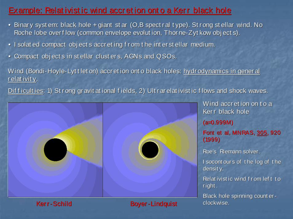
Example: Relativistic wind accretion onto a Kerr black holeExample: Relativistic wind accretion onto a Kerr black hole•• Binary system: black hole + giant star (O,B spectral type). StroBinary system: black hole + giant star (O,B spectral type). Strong stellar wind. No ng stellar wind. No

Roche lobe overflow (common envelope evolution, ThorneRoche lobe overflow (common envelope evolution, Thorne--Zytkow objects).Zytkow objects).

•• Isolated compact objects accreting from the interstellar medium.Isolated compact objects accreting from the interstellar medium.

•• Compact objects in stellar clusters, AGNs and QSOs.Compact objects in stellar clusters, AGNs and QSOs.

Wind (BondiWind (Bondi--HoyleHoyle--Lyttleton) accretion onto black holes: Lyttleton) accretion onto black holes: hydrodynamics in general hydrodynamics in general relativityrelativity..

DifficultiesDifficulties: 1) Strong gravitational fields, 2) Ultrarelativistic flows and: 1) Strong gravitational fields, 2) Ultrarelativistic flows and shock waves.shock waves.

Wind accretion on to a Wind accretion on to a Kerr black holeKerr black hole(a=0.999M)(a=0.999M)

Font et al, MNRAS, Font et al, MNRAS, 305305, 920 , 920 (1999)(1999)

Roe’s Riemann solver. Roe’s Riemann solver.

Isocontours of the log of the Isocontours of the log of the density. density.

Relativistic wind from left to Relativistic wind from left to right. right.

Black hole spinning counterBlack hole spinning counter--clockwise.clockwise.KerrKerr--Schild BoyerSchild Boyer--LindquistLindquist

Example: Relativistic rotating core collapse simulationExample: Relativistic rotating core collapse simulationFor movies of additional models visit:For movies of additional models visit:

www.mpawww.mpa--garching.mpg.de/rel_hydro/axi_core_collapse/movies.shtmlgarching.mpg.de/rel_hydro/axi_core_collapse/movies.shtml

Larger central densities in relativistic modelsLarger central densities in relativistic modelsSimilar gravitational radiation amplitudes (or smaller in the GRSimilar gravitational radiation amplitudes (or smaller in the GR case)case)

GR effects do not improve the chances for detection (at least inGR effects do not improve the chances for detection (at least inaxisymmetry):axisymmetry): Only a Galactic supernova (10 kpc) would be Only a Galactic supernova (10 kpc) would be detectable by the first generation of gravitational wave laser detectable by the first generation of gravitational wave laser interferometers.interferometers.Waveform catalogueWaveform catalogue:: www.mpawww.mpa--garching.mpg.de/rel_hydro/wave_catalogue.shtmlgarching.mpg.de/rel_hydro/wave_catalogue.shtml

Example: nonlinear pulsations of rotating neutron starsExample: nonlinear pulsations of rotating neutron starsDimmelmeierDimmelmeier, , StergioulasStergioulas & Font, MNRAS, submitted (2005)& Font, MNRAS, submitted (2005)

GRHD simulations show the appearance of nonlinear harmonicsGRHD simulations show the appearance of nonlinear harmonics of the linear pulsation of the linear pulsation modes: modes: linear sums and differenceslinear sums and differences of linear mode frequencies.of linear mode frequencies.

l=2 trial eigenfunctionl=2 trial eigenfunctionThe presence of The presence of nonlinear harmonicsnonlinear harmonics makes possible makes possible 33--mode couplingsmode couplings when the star is rotatingwhen the star is rotating, as , as different modes are affected in different ways by different modes are affected in different ways by rotation.rotation.

33--mode couplings could mode couplings could potentiallypotentially lead to resonance lead to resonance effects or (parametric) instabilities: effects or (parametric) instabilities: significant significant amount of energy from one mode could be amount of energy from one mode could be transferedtransfered to other modes. to other modes.

Best case scenarioBest case scenario: : PulsationalPulsational energy from the energy from the quasiquasi--radial mode (stored during core bounce) radial mode (stored during core bounce) transferedtransfered to stronger radiating to stronger radiating nonradialnonradial modes.modes.

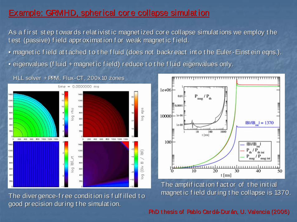
Example: GRMHD, spherical core collapse simulationExample: GRMHD, spherical core collapse simulation

As a first step towards relativistic magnetized core collapse siAs a first step towards relativistic magnetized core collapse simulations we employ the mulations we employ the test (passive) field approximation for weak magnetic field.test (passive) field approximation for weak magnetic field.

•• magnetic field attached to the fluid (does not backreact into tmagnetic field attached to the fluid (does not backreact into the Eulerhe Euler--Einstein eqns.).Einstein eqns.).

•• eigenvalues (fluid + magnetic field) reduce to the fluid eigenveigenvalues (fluid + magnetic field) reduce to the fluid eigenvalues only.alues only.

HLL solver + PPM, FluxHLL solver + PPM, Flux--CT, 200x10 zonesCT, 200x10 zones

The amplification factor of the initial The amplification factor of the initial magnetic field during the collapse is 1370.magnetic field during the collapse is 1370.The divergenceThe divergence--free condition is fulfilled to free condition is fulfilled to

good precision during the simulation.good precision during the simulation.PhD thesis of Pablo CerdáPhD thesis of Pablo Cerdá--Durán, U. Valencia (2006)Durán, U. Valencia (2006)

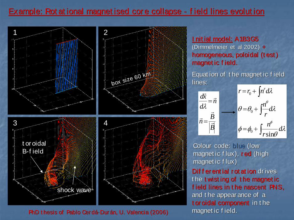
Example: Rotational Example: Rotational magnetisedmagnetised core collapse core collapse -- field lines evolutionfield lines evolution

Initial model:Initial model: A1B3G5A1B3G5(Dimmelmeier et al 2002)(Dimmelmeier et al 2002) + + homogeneous, poloidal (test) homogeneous, poloidal (test) magnetic field.magnetic field.

Equation of the magnetic field Equation of the magnetic field lines:lines:

11

33

22

44 BBn

ndxd

=

= λ

∫

∫

∫

+=

+=

+=

λθ

φφ

λθθ

λ

φ

θ

dr

n

drn

dnrr r

sin0

0

0

shock waveshock wave

toroidal toroidal BB--fieldfield

box size 60 kmbox size 60 km

Colour code: Colour code: blueblue (low (low magnetic flux), magnetic flux), redred (high (high magnetic flux)magnetic flux)Differential rotationDifferential rotation drives drives the the twisting of the magnetic twisting of the magnetic field lines in the nascent PNS, field lines in the nascent PNS, and the appearance of a and the appearance of a toroidal componenttoroidal component in the in the magnetic field.magnetic field.PhD thesis of Pablo CerdáPhD thesis of Pablo Cerdá--Durán, U. Valencia (2006)Durán, U. Valencia (2006)

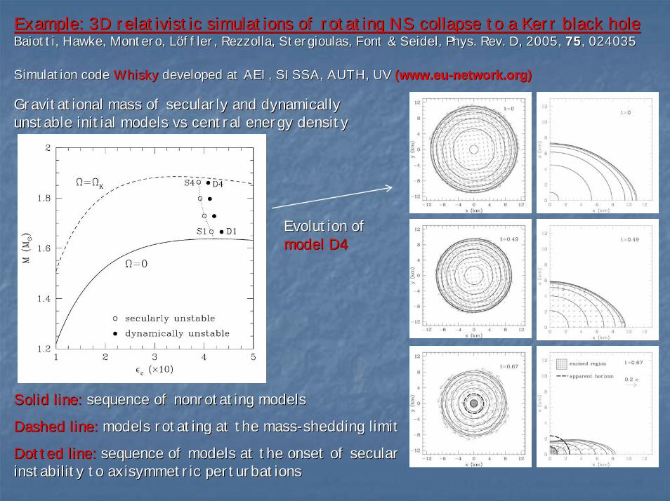
Example: 3D relativistic simulations of rotating NS collapse to Example: 3D relativistic simulations of rotating NS collapse to a Kerr black holea Kerr black holeBaiottiBaiotti, Hawke, Montero, , Hawke, Montero, LöfflerLöffler, , RezzollaRezzolla, , StergioulasStergioulas, Font & Seidel, Phys. Rev. D, 2005, , Font & Seidel, Phys. Rev. D, 2005, 7575, 024035, 024035

Simulation codeSimulation code WhiskyWhisky developed at AEI, SISSA, AUTH, UVdeveloped at AEI, SISSA, AUTH, UV ((www.euwww.eu--network.orgnetwork.org))

Gravitational mass of secularly and dynamically Gravitational mass of secularly and dynamically unstable initial models vs central energy densityunstable initial models vs central energy density

Evolution ofEvolution ofmodel D4model D4

Solid line:Solid line: sequence of nonrotating modelssequence of nonrotating models

Dashed line:Dashed line: models rotating at the massmodels rotating at the mass--shedding limitshedding limit

Dotted line:Dotted line: sequence of models at the onset of secular sequence of models at the onset of secular instability to axisymmetric perturbationsinstability to axisymmetric perturbations

Calculating apparent and event horizonsCalculating apparent and event horizonsGrey surface: Grey surface: event horizonevent horizon. White surface: . White surface: apparent horizonapparent horizon. Circles: . Circles: horizon generatorshorizon generators

Calculations and visualization by P. Calculations and visualization by P. DienerDiener (AEI/LSU)(AEI/LSU)

event horizonevent horizon

apparent horizonapparent horizon

stellar surfacestellar surface

As the collapse proceeds, trapped surfaces form (photons cannot As the collapse proceeds, trapped surfaces form (photons cannot leave). leave).

Most relevant surfaces are the Most relevant surfaces are the apparent horizonapparent horizon (outermost of the trapped surfaces) (outermost of the trapped surfaces) and the and the event horizonevent horizon (global null surface).(global null surface).

AH can be computed at any time (zero expansion of a photon congAH can be computed at any time (zero expansion of a photon congruence). EH requires ruence). EH requires the construction of the whole the construction of the whole spacetimespacetime..

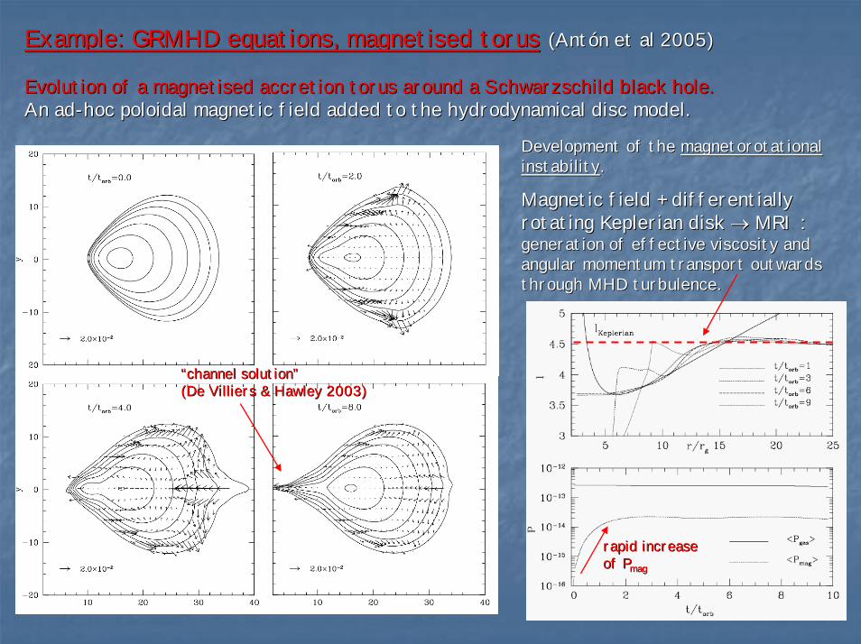
Example: GRMHD equations, Example: GRMHD equations, magnetisedmagnetised torustorus ((AntónAntón et al 2005)et al 2005)

Evolution of a magnetised accretion torus around a SchwarzschildEvolution of a magnetised accretion torus around a Schwarzschild black hole.black hole.An adAn ad--hoc poloidal magnetic field added to the hydrodynamical disc modhoc poloidal magnetic field added to the hydrodynamical disc model.el.

Development of the Development of the magnetorotational magnetorotational instabilityinstability..

Magnetic field + differentially Magnetic field + differentially rotating Keplerian disk rotating Keplerian disk →→ MRI : MRI : generation of effective viscosity and generation of effective viscosity and angular momentum transport outwards angular momentum transport outwards through MHD turbulence.through MHD turbulence.

rapid increase rapid increase of Pof Pmagmag

““channel solution” channel solution” (De Villiers & Hawley 2003)(De Villiers & Hawley 2003)

General Relativistic Magnetohydrodynamic Simulations of AccretioGeneral Relativistic Magnetohydrodynamic Simulations of Accretion Torin ToriSchwarzschild BH, development of the Schwarzschild BH, development of the magnetorotational instabilitymagnetorotational instability..

Magnetic field + differentially rotating Keplerian disk Magnetic field + differentially rotating Keplerian disk →→ MRI :MRI : generation of effective generation of effective viscosity and angular momentum transport outwards through MHD tuviscosity and angular momentum transport outwards through MHD turbulence.rbulence.

For further animations visit:For further animations visit:http://www.astro.virginia.edu/~jd5v/

De Villiers & Hawley (2003)De Villiers & Hawley (2003)http://www.astro.virginia.edu/~jd5v/

Example: Binary neutron star coalescence. Simulations with realiExample: Binary neutron star coalescence. Simulations with realistic EOSstic EOSShibata, Taniguchi & Uryu, 2005, Phys. Rev. D, 71, 084021Shibata, Taniguchi & Uryu, 2005, Phys. Rev. D, 71, 084021

Shibata & Font, 2005, Phys. Rev. D, 72, Shibata & Font, 2005, Phys. Rev. D, 72,

1.4M1.4Msunsun -- 1.4M1.4Msun sun casecase

Prompt formation of a rotating black hole Prompt formation of a rotating black hole 1.25M1.25Msunsun -- 1.35M1.35Msun sun casecase

Formation of a differentially rotating Formation of a differentially rotating hypermassive neutron starhypermassive neutron star

QuasiQuasi--periodic, large amplitude gravitational waves are emitted, with periodic, large amplitude gravitational waves are emitted, with frequencies frequencies between 3between 3--4 kHz during 4 kHz during ~ 100 ms~ 100 ms (after which the NS collapses to a BH). (after which the NS collapses to a BH).

Those waves could be detected by LIGOThose waves could be detected by LIGO--II up to distances of II up to distances of ~ 100 ~ 100 MpcMpc..

Summary of the talkSummary of the talk

• Conservative formulations of the GRHD/GRMHD equationsConservative formulations of the GRHD/GRMHD equations currently available.currently available.

•• HighHigh--resolution shockresolution shock--capturing numerical schemescapturing numerical schemes based on the wave structure of those based on the wave structure of those hyperbolic systems developed in recent years.hyperbolic systems developed in recent years.

•• GRHD simulationsGRHD simulations in relativistic astrophysics in relativistic astrophysics routinely performedroutinely performed nowadays within the nowadays within the soso--called called “test“test--fluid” approximation.fluid” approximation.

•• Important advances also achieved for the Important advances also achieved for the GRMHD caseGRMHD case, but the , but the full development still full development still awaits for a thorough numerical exploration.awaits for a thorough numerical exploration.

•• LongLong--term stable formulations of the full Einstein equationsterm stable formulations of the full Einstein equations (or accurate enough (or accurate enough approximations) have been proposed by several Numerical Relativiapproximations) have been proposed by several Numerical Relativity groups.ty groups.

•• Stable, coupled evolutions (GRHD/GRMHD + Einstein equations) areStable, coupled evolutions (GRHD/GRMHD + Einstein equations) are becoming possible in becoming possible in 3D3D, allowing for the study of interesting relativistic astrophysic, allowing for the study of interesting relativistic astrophysics scenarios (e.g. s scenarios (e.g. gravitational collapse, accretion, binary neutron star mergers).gravitational collapse, accretion, binary neutron star mergers).