an introduction to numpy and scipy -...

© 2012 M. Scott Shell 1/24 last modified 3/22/2012

An introduction to Numpy and Scipy

Table of contents

Table of contents ............................................................................................................................ 1

Overview ......................................................................................................................................... 2

Installation ...................................................................................................................................... 2

Other resources .............................................................................................................................. 2

Importing the NumPy module ........................................................................................................ 2

Arrays .............................................................................................................................................. 3

Other ways to create arrays............................................................................................................ 7

Array mathematics .......................................................................................................................... 8

Array iteration ............................................................................................................................... 10

Basic array operations .................................................................................................................. 11

Comparison operators and value testing ..................................................................................... 12

Array item selection and manipulation ........................................................................................ 14

Vector and matrix mathematics ................................................................................................... 16

Polynomial mathematics .............................................................................................................. 18

Statistics ........................................................................................................................................ 19

Random numbers .......................................................................................................................... 19

Other functions to know about .................................................................................................... 21

Modules available in SciPy ............................................................................................................ 21


Overview

NumPy and SciPy are open-source add-on modules to Python that provide common

mathematical and numerical routines in pre-compiled, fast functions. These are growing into

highly mature packages that provide functionality that meets, or perhaps exceeds, that

associated with common commercial software like MatLab. The NumPy (Numeric Python)

package provides basic routines for manipulating large arrays and matrices of numeric data.

The SciPy (Scientific Python) package extends the functionality of NumPy with a substantial

collection of useful algorithms, like minimization, Fourier transformation, regression, and other

applied mathematical techniques.

Installation

If you installed Python(x,y) on a Windows platform, then you should be ready to go. If not, then

you will have to install these add-ons manually after installing Python, in the order of NumPy

and then SciPy. Installation files are available for both at:

http://www.scipy.org/Download

Follow links on this page to download the official releases, which will be in the form of .exe

install files for Windows and .dmg install files for MacOS.

Other resources

The NumPy and SciPy development community maintains an extensive online documentation

system, including user guides and tutorials, at:

http://docs.scipy.org/doc/

Importing the NumPy module

There are several ways to import NumPy. The standard approach is to use a simple import

statement:

>>> import numpy

However, for large amounts of calls to NumPy functions, it can become tedious to write

numpy.X over and over again. Instead, it is common to import under the briefer name np:

>>> import numpy as np


This statement will allow us to access NumPy objects using np.X instead of numpy.X. It is

also possible to import NumPy directly into the current namespace so that we don't have to use

dot notation at all, but rather simply call the functions as if they were built-in:

>>> from numpy import *

However, this strategy is usually frowned upon in Python programming because it starts to

remove some of the nice organization that modules provide. For the remainder of this tutorial,

we will assume that the import numpy as np has been used.

Arrays

The central feature of NumPy is the array object class. Arrays are similar to lists in Python,

except that every element of an array must be of the same type, typically a numeric type like

float or int. Arrays make operations with large amounts of numeric data very fast and are

generally much more efficient than lists.

An array can be created from a list:

>>> a = np.array([1, 4, 5, 8], float) >>> a array([ 1., 4., 5., 8.]) >>> type(a) <type 'numpy.ndarray'>

Here, the function array takes two arguments: the list to be converted into the array and the

type of each member of the list. Array elements are accessed, sliced, and manipulated just like

lists:

>>> a[:2] array([ 1., 4.]) >>> a[3] 8.0 >>> a[0] = 5. >>> a array([ 5., 4., 5., 8.])

Arrays can be multidimensional. Unlike lists, different axes are accessed using commas inside

bracket notation. Here is an example with a two-dimensional array (e.g., a matrix):

>>> a = np.array([[1, 2, 3], [4, 5, 6]], float) >>> a array([[ 1., 2., 3.], [ 4., 5., 6.]]) >>> a[0,0] 1.0 >>> a[0,1] 2.0


Array slicing works with multiple dimensions in the same way as usual, applying each slice

specification as a filter to a specified dimension. Use of a single ":" in a dimension indicates the

use of everything along that dimension:

>>> a = np.array([[1, 2, 3], [4, 5, 6]], float) >>> a[1,:] array([ 4., 5., 6.]) >>> a[:,2] array([ 3., 6.]) >>> a[-1:,-2:] array([[ 5., 6.]])

The shape property of an array returns a tuple with the size of each array dimension:

>>> a.shape (2, 3)

The dtype property tells you what type of values are stored by the array:

>>> a.dtype dtype('float64')

Here, float64 is a numeric type that NumPy uses to store double-precision (8-byte) real

numbers, similar to the float type in Python.

When used with an array, the len function returns the length of the first axis:

>>> a = np.array([[1, 2, 3], [4, 5, 6]], float) >>> len(a) 2

The in statement can be used to test if values are present in an array:

>>> a = np.array([[1, 2, 3], [4, 5, 6]], float) >>> 2 in a True >>> 0 in a False

Arrays can be reshaped using tuples that specify new dimensions. In the following example, we

turn a ten-element one-dimensional array into a two-dimensional one whose first axis has five

elements and whose second axis has two elements:

>>> a = np.array(range(10), float) >>> a array([ 0., 1., 2., 3., 4., 5., 6., 7., 8., 9.]) >>> a = a.reshape((5, 2)) >>> a array([[ 0., 1.], [ 2., 3.],


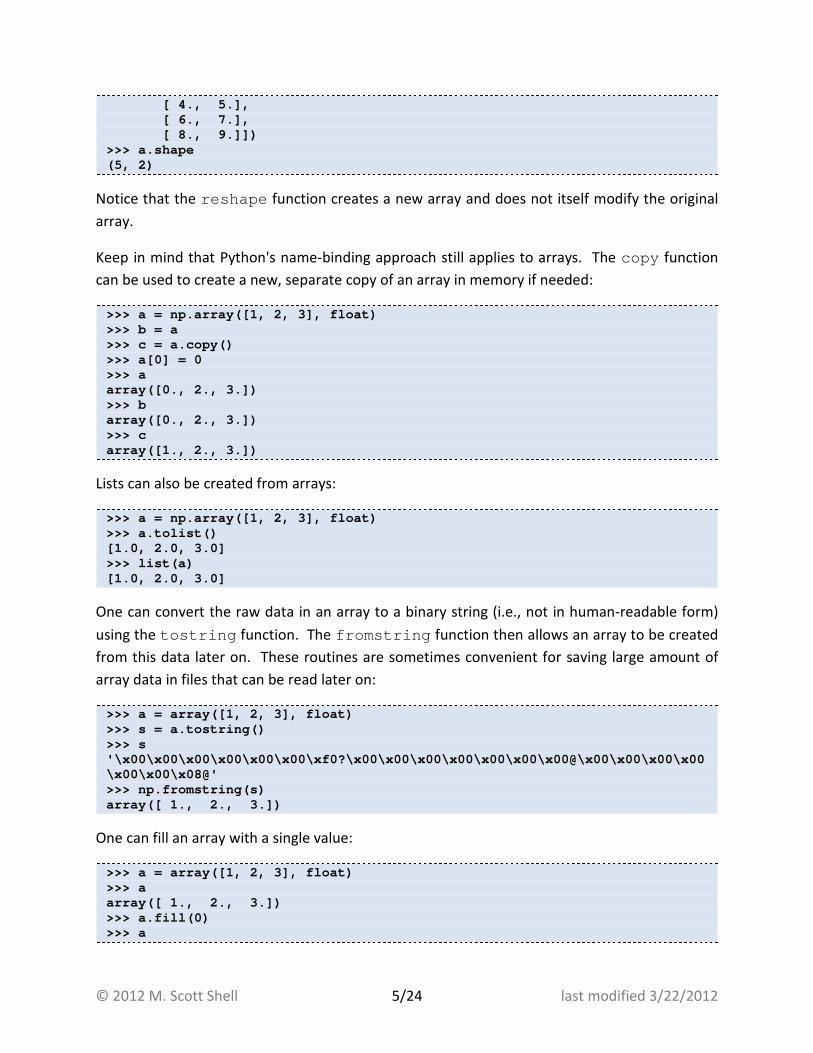
[ 4., 5.], [ 6., 7.], [ 8., 9.]]) >>> a.shape (5, 2)

Notice that the reshape function creates a new array and does not itself modify the original

array.

Keep in mind that Python's name-binding approach still applies to arrays. The copy function

can be used to create a new, separate copy of an array in memory if needed:

>>> a = np.array([1, 2, 3], float) >>> b = a >>> c = a.copy() >>> a[0] = 0 >>> a array([0., 2., 3.]) >>> b array([0., 2., 3.]) >>> c array([1., 2., 3.])

Lists can also be created from arrays:

>>> a = np.array([1, 2, 3], float) >>> a.tolist() [1.0, 2.0, 3.0] >>> list(a) [1.0, 2.0, 3.0]

One can convert the raw data in an array to a binary string (i.e., not in human-readable form)

using the tostring function. The fromstring function then allows an array to be created

from this data later on. These routines are sometimes convenient for saving large amount of

array data in files that can be read later on:

>>> a = array([1, 2, 3], float) >>> s = a.tostring() >>> s '\x00\x00\x00\x00\x00\x00\xf0?\x00\x00\x00\x00\x00\ x00\x00@\x00\x00\x00\x00\x00\x00\x08@' >>> np.fromstring(s) array([ 1., 2., 3.])

One can fill an array with a single value:

>>> a = array([1, 2, 3], float) >>> a array([ 1., 2., 3.]) >>> a.fill(0) >>> a


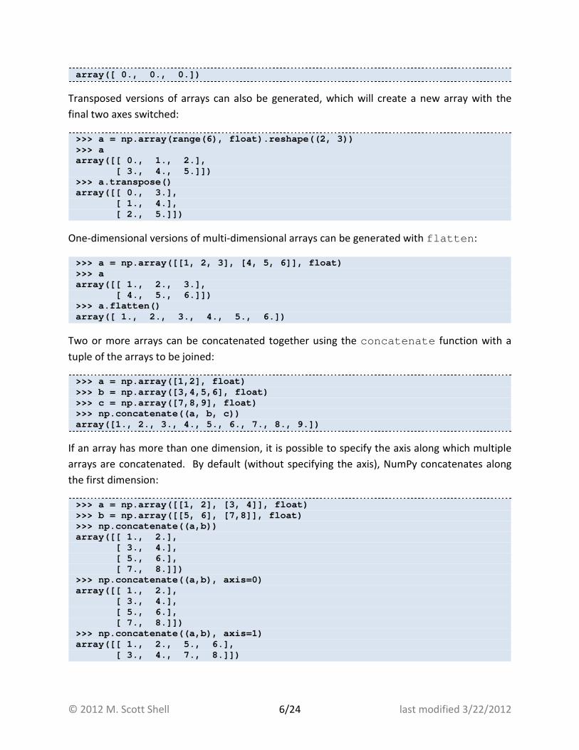
array([ 0., 0., 0.])

Transposed versions of arrays can also be generated, which will create a new array with the

final two axes switched:

>>> a = np.array(range(6), float).reshape((2, 3)) >>> a array([[ 0., 1., 2.], [ 3., 4., 5.]]) >>> a.transpose() array([[ 0., 3.], [ 1., 4.], [ 2., 5.]])

One-dimensional versions of multi-dimensional arrays can be generated with flatten:

>>> a = np.array([[1, 2, 3], [4, 5, 6]], float) >>> a array([[ 1., 2., 3.], [ 4., 5., 6.]]) >>> a.flatten() array([ 1., 2., 3., 4., 5., 6.])

Two or more arrays can be concatenated together using the concatenate function with a

tuple of the arrays to be joined:

>>> a = np.array([1,2], float) >>> b = np.array([3,4,5,6], float) >>> c = np.array([7,8,9], float) >>> np.concatenate((a, b, c)) array([1., 2., 3., 4., 5., 6., 7., 8., 9.])

If an array has more than one dimension, it is possible to specify the axis along which multiple

arrays are concatenated. By default (without specifying the axis), NumPy concatenates along

the first dimension:

>>> a = np.array([[1, 2], [3, 4]], float) >>> b = np.array([[5, 6], [7,8]], float) >>> np.concatenate((a,b)) array([[ 1., 2.], [ 3., 4.], [ 5., 6.], [ 7., 8.]]) >>> np.concatenate((a,b), axis=0) array([[ 1., 2.], [ 3., 4.], [ 5., 6.], [ 7., 8.]]) >>> np.concatenate((a,b), axis=1) array([[ 1., 2., 5., 6.], [ 3., 4., 7., 8.]])


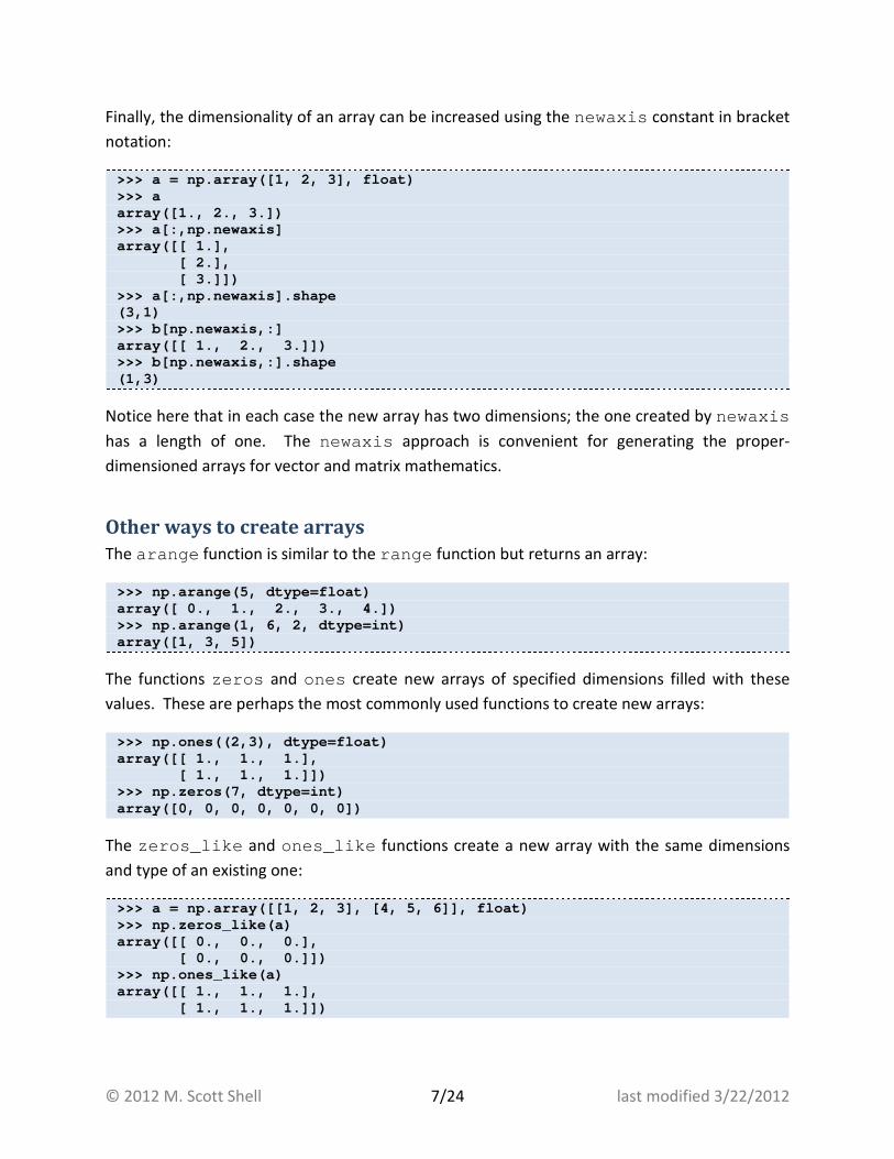
Finally, the dimensionality of an array can be increased using the newaxis constant in bracket

notation:

>>> a = np.array([1, 2, 3], float) >>> a array([1., 2., 3.]) >>> a[:,np.newaxis] array([[ 1.], [ 2.], [ 3.]]) >>> a[:,np.newaxis].shape (3,1) >>> b[np.newaxis,:] array([[ 1., 2., 3.]]) >>> b[np.newaxis,:].shape (1,3)

Notice here that in each case the new array has two dimensions; the one created by newaxis

has a length of one. The newaxis approach is convenient for generating the proper-

dimensioned arrays for vector and matrix mathematics.

Other ways to create arrays

The arange function is similar to the range function but returns an array:

>>> np.arange(5, dtype=float) array([ 0., 1., 2., 3., 4.]) >>> np.arange(1, 6, 2, dtype=int) array([1, 3, 5])

The functions zeros and ones create new arrays of specified dimensions filled with these

values. These are perhaps the most commonly used functions to create new arrays:

>>> np.ones((2,3), dtype=float) array([[ 1., 1., 1.], [ 1., 1., 1.]]) >>> np.zeros(7, dtype=int) array([0, 0, 0, 0, 0, 0, 0])

The zeros_like and ones_like functions create a new array with the same dimensions

and type of an existing one:

>>> a = np.array([[1, 2, 3], [4, 5, 6]], float) >>> np.zeros_like(a) array([[ 0., 0., 0.], [ 0., 0., 0.]]) >>> np.ones_like(a) array([[ 1., 1., 1.], [ 1., 1., 1.]])


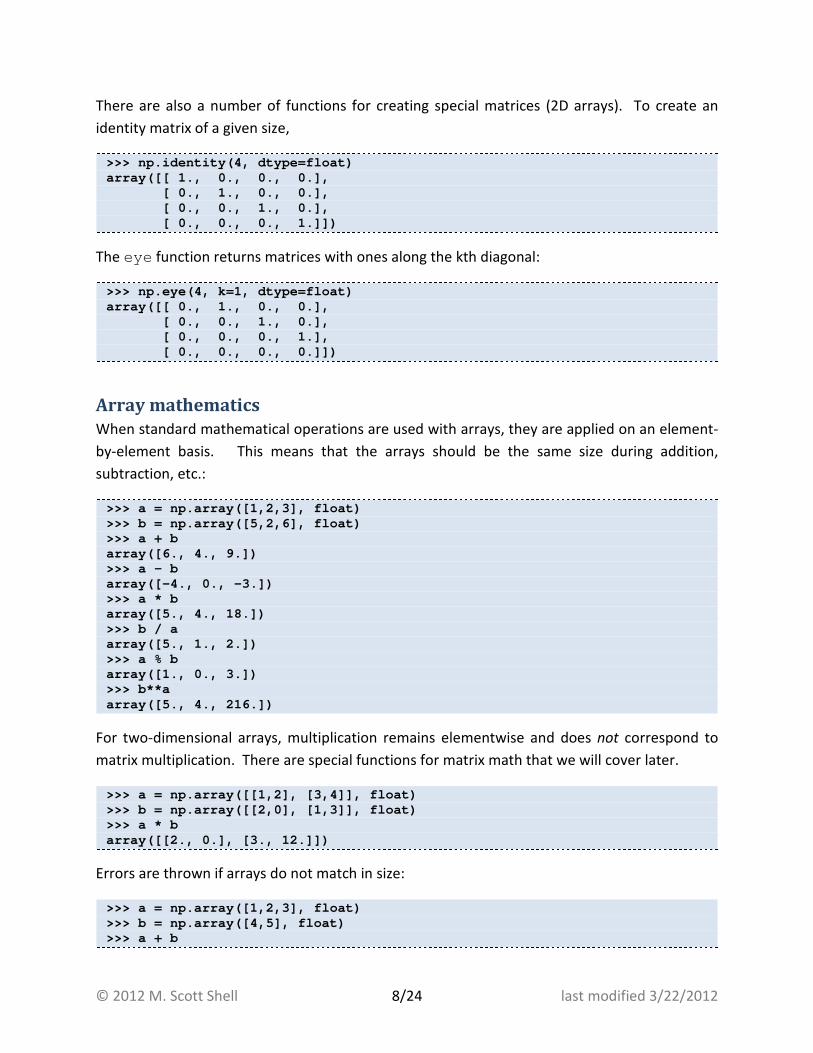
There are also a number of functions for creating special matrices (2D arrays). To create an

identity matrix of a given size,

>>> np.identity(4, dtype=float) array([[ 1., 0., 0., 0.], [ 0., 1., 0., 0.], [ 0., 0., 1., 0.], [ 0., 0., 0., 1.]])

The eye function returns matrices with ones along the kth diagonal:

>>> np.eye(4, k=1, dtype=float) array([[ 0., 1., 0., 0.], [ 0., 0., 1., 0.], [ 0., 0., 0., 1.], [ 0., 0., 0., 0.]])

Array mathematics

When standard mathematical operations are used with arrays, they are applied on an element-

by-element basis. This means that the arrays should be the same size during addition,

subtraction, etc.:

>>> a = np.array([1,2,3], float) >>> b = np.array([5,2,6], float) >>> a + b array([6., 4., 9.]) >>> a – b array([-4., 0., -3.]) >>> a * b array([5., 4., 18.]) >>> b / a array([5., 1., 2.]) >>> a % b array([1., 0., 3.]) >>> b**a array([5., 4., 216.])

For two-dimensional arrays, multiplication remains elementwise and does not correspond to

matrix multiplication. There are special functions for matrix math that we will cover later.

>>> a = np.array([[1,2], [3,4]], float) >>> b = np.array([[2,0], [1,3]], float) >>> a * b array([[2., 0.], [3., 12.]])

Errors are thrown if arrays do not match in size:

>>> a = np.array([1,2,3], float) >>> b = np.array([4,5], float) >>> a + b


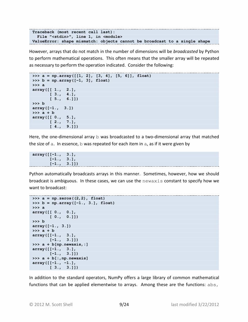
Traceback (most recent call last): File "<stdin>", line 1, in <module> ValueError: shape mismatch: objects cannot be broad cast to a single shape

However, arrays that do not match in the number of dimensions will be broadcasted by Python

to perform mathematical operations. This often means that the smaller array will be repeated

as necessary to perform the operation indicated. Consider the following:

>>> a = np.array([[1, 2], [3, 4], [5, 6]], float) >>> b = np.array([-1, 3], float) >>> a array([[ 1., 2.], [ 3., 4.], [ 5., 6.]]) >>> b array([-1., 3.]) >>> a + b array([[ 0., 5.], [ 2., 7.], [ 4., 9.]])

Here, the one-dimensional array b was broadcasted to a two-dimensional array that matched

the size of a. In essence, b was repeated for each item in a, as if it were given by

array([[-1., 3.], [-1., 3.], [-1., 3.]])

Python automatically broadcasts arrays in this manner. Sometimes, however, how we should

broadcast is ambiguous. In these cases, we can use the newaxis constant to specify how we

want to broadcast:

>>> a = np.zeros((2,2), float) >>> b = np.array([-1., 3.], float) >>> a array([[ 0., 0.], [ 0., 0.]]) >>> b array([-1., 3.]) >>> a + b array([[-1., 3.], [-1., 3.]]) >>> a + b[np.newaxis,:] array([[-1., 3.], [-1., 3.]]) >>> a + b[:,np.newaxis] array([[-1., -1.], [ 3., 3.]])

In addition to the standard operators, NumPy offers a large library of common mathematical

functions that can be applied elementwise to arrays. Among these are the functions: abs,


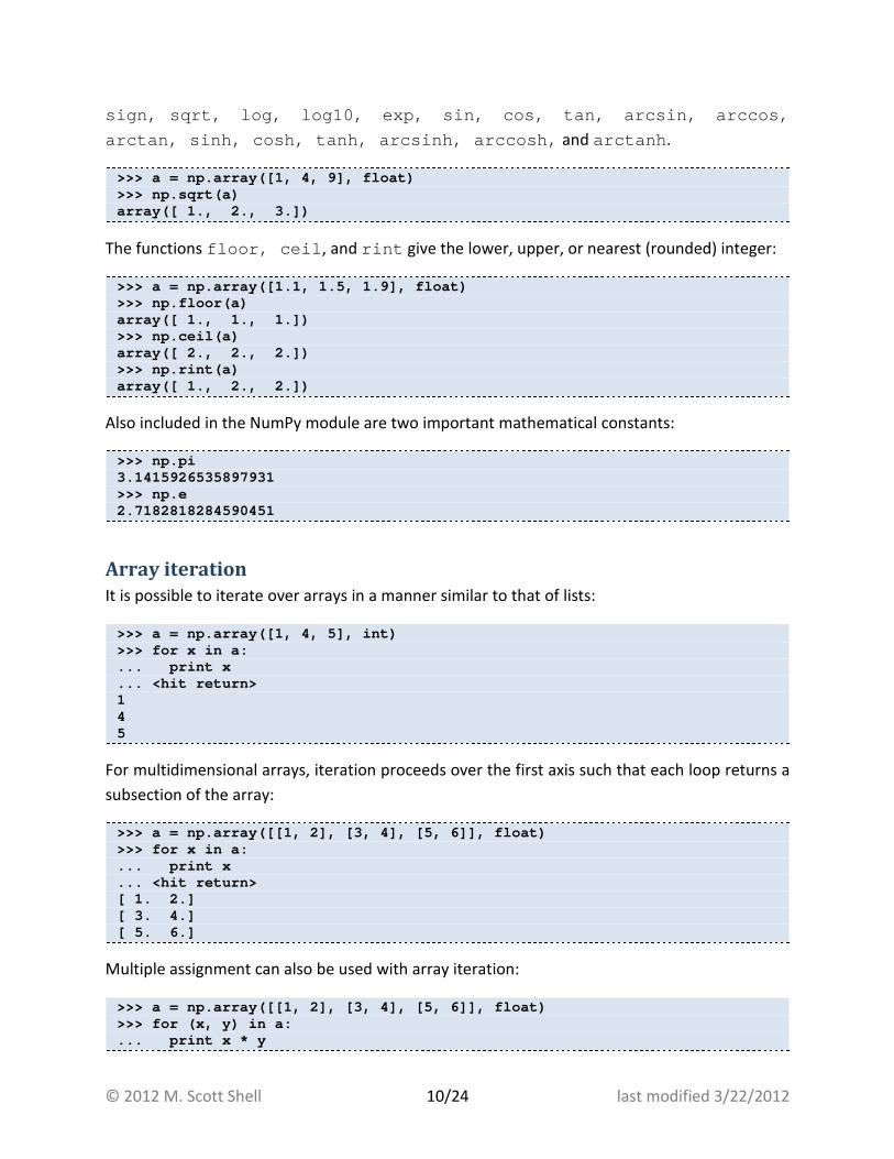
sign, sqrt, log, log10, exp, sin, cos, tan, arcsin, arccos,

arctan, sinh, cosh, tanh, arcsinh, arccosh, and arctanh.

>>> a = np.array([1, 4, 9], float) >>> np.sqrt(a) array([ 1., 2., 3.])

The functions floor, ceil, and rint give the lower, upper, or nearest (rounded) integer:

>>> a = np.array([1.1, 1.5, 1.9], float) >>> np.floor(a) array([ 1., 1., 1.]) >>> np.ceil(a) array([ 2., 2., 2.]) >>> np.rint(a) array([ 1., 2., 2.])

Also included in the NumPy module are two important mathematical constants:

>>> np.pi 3.1415926535897931 >>> np.e 2.7182818284590451

Array iteration

It is possible to iterate over arrays in a manner similar to that of lists:

>>> a = np.array([1, 4, 5], int) >>> for x in a: ... print x ... <hit return> 1 4 5

For multidimensional arrays, iteration proceeds over the first axis such that each loop returns a

subsection of the array:

>>> a = np.array([[1, 2], [3, 4], [5, 6]], float) >>> for x in a: ... print x ... <hit return> [ 1. 2.] [ 3. 4.] [ 5. 6.]

Multiple assignment can also be used with array iteration:

>>> a = np.array([[1, 2], [3, 4], [5, 6]], float) >>> for (x, y) in a: ... print x * y


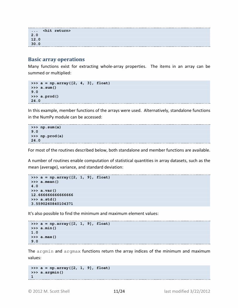
... <hit return> 2.0 12.0 30.0

Basic array operations

Many functions exist for extracting whole-array properties. The items in an array can be

summed or multiplied:

>>> a = np.array([2, 4, 3], float) >>> a.sum() 9.0 >>> a.prod() 24.0

In this example, member functions of the arrays were used. Alternatively, standalone functions

in the NumPy module can be accessed:

>>> np.sum(a) 9.0 >>> np.prod(a) 24.0

For most of the routines described below, both standalone and member functions are available.

A number of routines enable computation of statistical quantities in array datasets, such as the

mean (average), variance, and standard deviation:

>>> a = np.array([2, 1, 9], float) >>> a.mean() 4.0 >>> a.var() 12.666666666666666 >>> a.std() 3.5590260840104371

It's also possible to find the minimum and maximum element values:

>>> a = np.array([2, 1, 9], float) >>> a.min() 1.0 >>> a.max() 9.0

The argmin and argmax functions return the array indices of the minimum and maximum

values:

>>> a = np.array([2, 1, 9], float) >>> a.argmin() 1


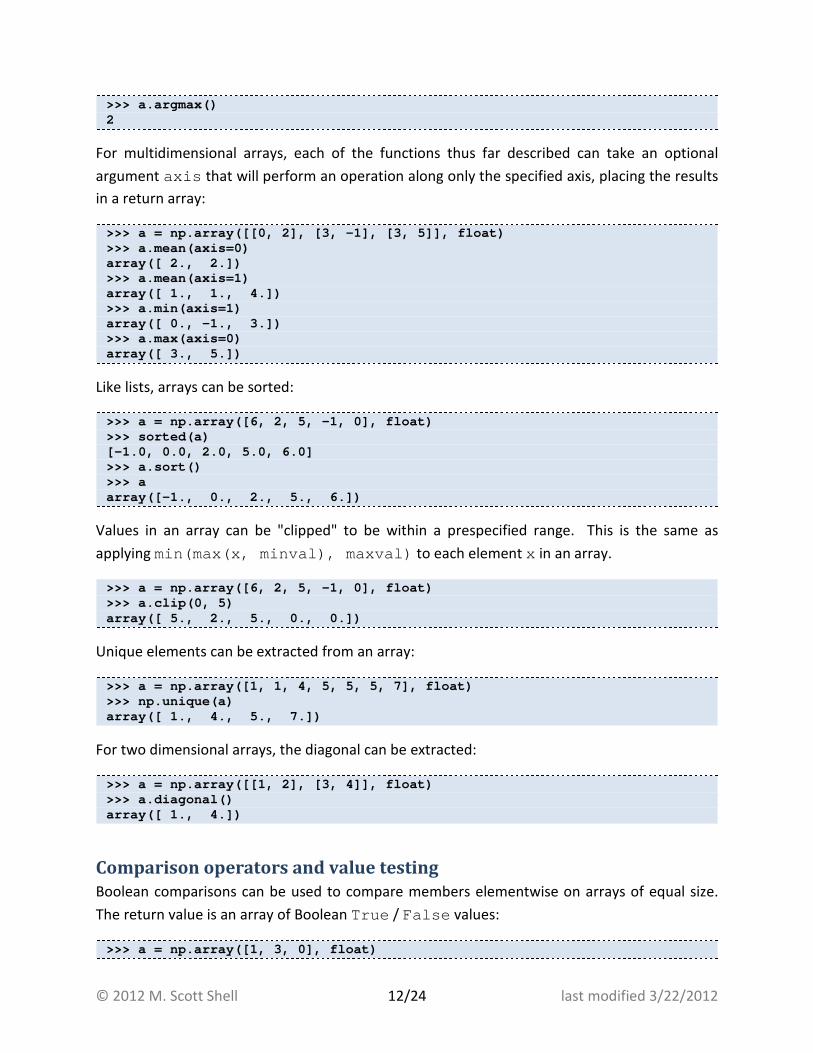
>>> a.argmax() 2

For multidimensional arrays, each of the functions thus far described can take an optional

argument axis that will perform an operation along only the specified axis, placing the results

in a return array:

>>> a = np.array([[0, 2], [3, -1], [3, 5]], float) >>> a.mean(axis=0) array([ 2., 2.]) >>> a.mean(axis=1) array([ 1., 1., 4.]) >>> a.min(axis=1) array([ 0., -1., 3.]) >>> a.max(axis=0) array([ 3., 5.])

Like lists, arrays can be sorted:

>>> a = np.array([6, 2, 5, -1, 0], float) >>> sorted(a) [-1.0, 0.0, 2.0, 5.0, 6.0] >>> a.sort() >>> a array([-1., 0., 2., 5., 6.])

Values in an array can be "clipped" to be within a prespecified range. This is the same as

applying min(max(x, minval), maxval) to each element x in an array.

>>> a = np.array([6, 2, 5, -1, 0], float) >>> a.clip(0, 5) array([ 5., 2., 5., 0., 0.])

Unique elements can be extracted from an array:

>>> a = np.array([1, 1, 4, 5, 5, 5, 7], float) >>> np.unique(a) array([ 1., 4., 5., 7.])

For two dimensional arrays, the diagonal can be extracted:

>>> a = np.array([[1, 2], [3, 4]], float) >>> a.diagonal() array([ 1., 4.])

Comparison operators and value testing

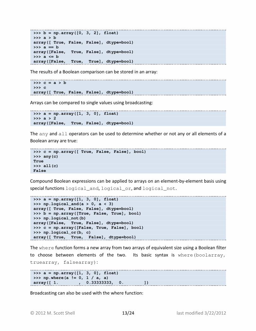
Boolean comparisons can be used to compare members elementwise on arrays of equal size.

The return value is an array of Boolean True / False values:

>>> a = np.array([1, 3, 0], float)


>>> b = np.array([0, 3, 2], float) >>> a > b array([ True, False, False], dtype=bool) >>> a == b array([False, True, False], dtype=bool) >>> a <= b array([False, True, True], dtype=bool)

The results of a Boolean comparison can be stored in an array:

>>> c = a > b >>> c array([ True, False, False], dtype=bool)

Arrays can be compared to single values using broadcasting:

>>> a = np.array([1, 3, 0], float) >>> a > 2 array([False, True, False], dtype=bool)

The any and all operators can be used to determine whether or not any or all elements of a

Boolean array are true:

>>> c = np.array([ True, False, False], bool) >>> any(c) True >>> all(c) False

Compound Boolean expressions can be applied to arrays on an element-by-element basis using

special functions logical_and, logical_or, and logical_not.

>>> a = np.array([1, 3, 0], float) >>> np.logical_and(a > 0, a < 3) array([ True, False, False], dtype=bool) >>> b = np.array([True, False, True], bool) >>> np.logical_not(b) array([False, True, False], dtype=bool) >>> c = np.array([False, True, False], bool) >>> np.logical_or(b, c) array([ True, True, False], dtype=bool)

The where function forms a new array from two arrays of equivalent size using a Boolean filter

to choose between elements of the two. Its basic syntax is where(boolarray,

truearray, falsearray):

>>> a = np.array([1, 3, 0], float) >>> np.where(a != 0, 1 / a, a) array([ 1. , 0.33333333, 0. ])

Broadcasting can also be used with the where function:


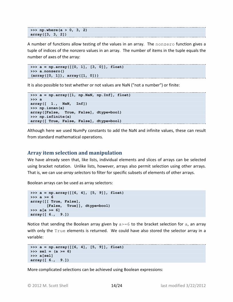
>>> np.where(a > 0, 3, 2) array([3, 3, 2])

A number of functions allow testing of the values in an array. The nonzero function gives a

tuple of indices of the nonzero values in an array. The number of items in the tuple equals the

number of axes of the array:

>>> a = np.array([[0, 1], [3, 0]], float) >>> a.nonzero() (array([0, 1]), array([1, 0]))

It is also possible to test whether or not values are NaN ("not a number") or finite:

>>> a = np.array([1, np.NaN, np.Inf], float) >>> a array([ 1., NaN, Inf]) >>> np.isnan(a) array([False, True, False], dtype=bool) >>> np.isfinite(a) array([ True, False, False], dtype=bool)

Although here we used NumPy constants to add the NaN and infinite values, these can result

from standard mathematical operations.

Array item selection and manipulation

We have already seen that, like lists, individual elements and slices of arrays can be selected

using bracket notation. Unlike lists, however, arrays also permit selection using other arrays.

That is, we can use array selectors to filter for specific subsets of elements of other arrays.

Boolean arrays can be used as array selectors:

>>> a = np.array([[6, 4], [5, 9]], float) >>> a >= 6 array([[ True, False], [False, True]], dtype=bool) >>> a[a >= 6] array([ 6., 9.])

Notice that sending the Boolean array given by a>=6 to the bracket selection for a, an array

with only the True elements is returned. We could have also stored the selector array in a

variable:

>>> a = np.array([[6, 4], [5, 9]], float) >>> sel = (a >= 6) >>> a[sel] array([ 6., 9.])

More complicated selections can be achieved using Boolean expressions:


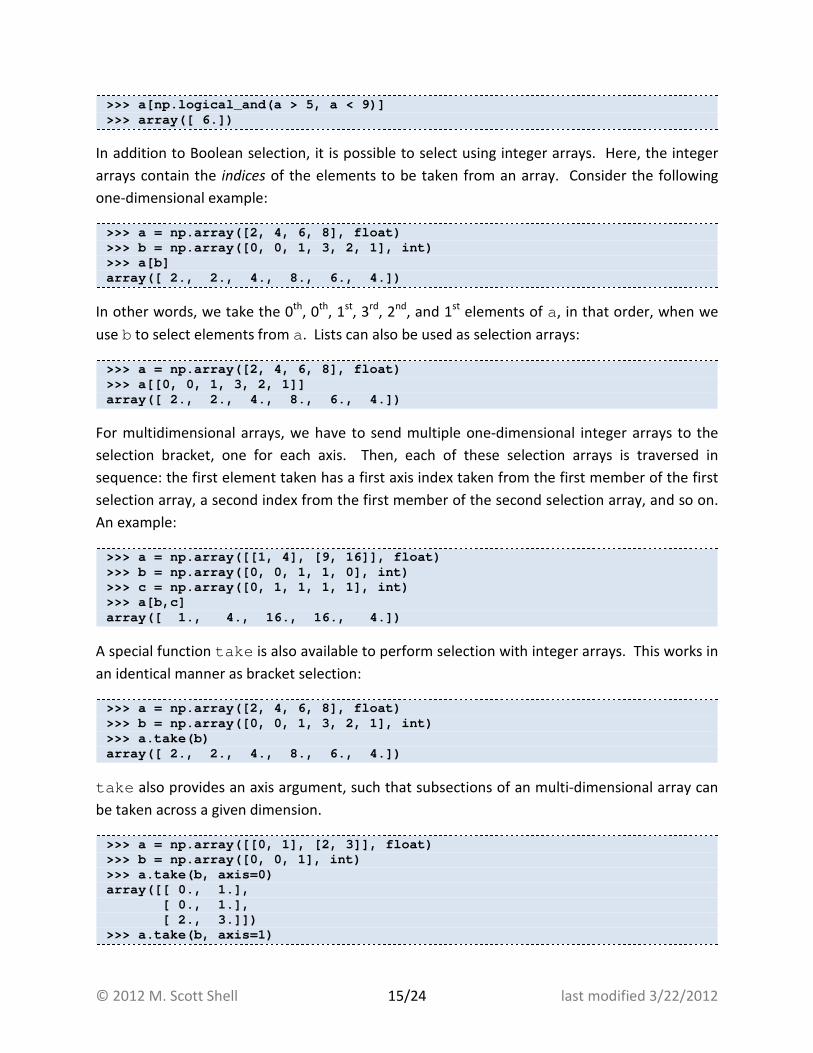
>>> a[np.logical_and(a > 5, a < 9)] >>> array([ 6.])

In addition to Boolean selection, it is possible to select using integer arrays. Here, the integer

arrays contain the indices of the elements to be taken from an array. Consider the following

one-dimensional example:

>>> a = np.array([2, 4, 6, 8], float) >>> b = np.array([0, 0, 1, 3, 2, 1], int) >>> a[b] array([ 2., 2., 4., 8., 6., 4.])

In other words, we take the 0th

, 0th

, 1st

, 3rd

, 2nd

, and 1st

elements of a, in that order, when we

use b to select elements from a. Lists can also be used as selection arrays:

>>> a = np.array([2, 4, 6, 8], float) >>> a[[0, 0, 1, 3, 2, 1]] array([ 2., 2., 4., 8., 6., 4.])

For multidimensional arrays, we have to send multiple one-dimensional integer arrays to the

selection bracket, one for each axis. Then, each of these selection arrays is traversed in

sequence: the first element taken has a first axis index taken from the first member of the first

selection array, a second index from the first member of the second selection array, and so on.

An example:

>>> a = np.array([[1, 4], [9, 16]], float) >>> b = np.array([0, 0, 1, 1, 0], int) >>> c = np.array([0, 1, 1, 1, 1], int) >>> a[b,c] array([ 1., 4., 16., 16., 4.])

A special function take is also available to perform selection with integer arrays. This works in

an identical manner as bracket selection:

>>> a = np.array([2, 4, 6, 8], float) >>> b = np.array([0, 0, 1, 3, 2, 1], int) >>> a.take(b) array([ 2., 2., 4., 8., 6., 4.])

take also provides an axis argument, such that subsections of an multi-dimensional array can

be taken across a given dimension.

>>> a = np.array([[0, 1], [2, 3]], float) >>> b = np.array([0, 0, 1], int) >>> a.take(b, axis=0) array([[ 0., 1.], [ 0., 1.], [ 2., 3.]]) >>> a.take(b, axis=1)


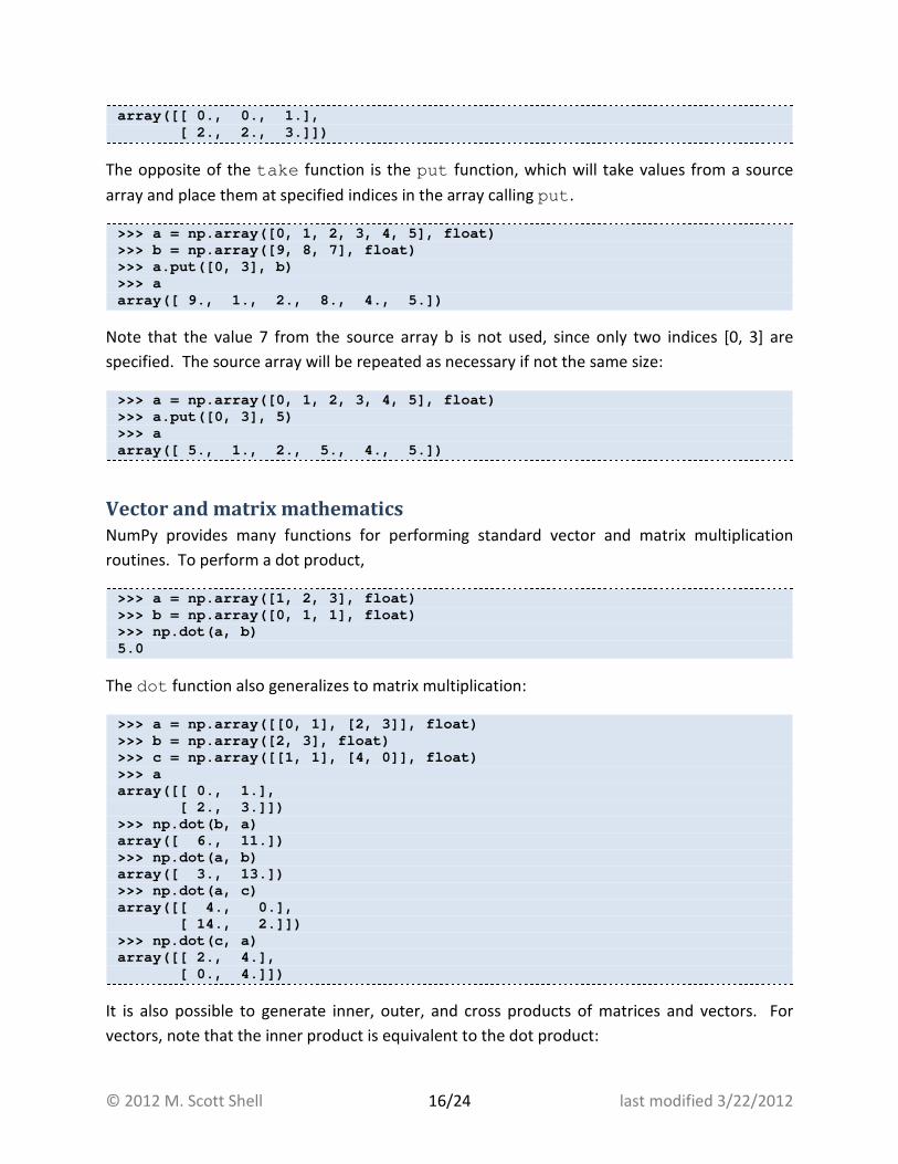
array([[ 0., 0., 1.], [ 2., 2., 3.]])

The opposite of the take function is the put function, which will take values from a source

array and place them at specified indices in the array calling put.

>>> a = np.array([0, 1, 2, 3, 4, 5], float) >>> b = np.array([9, 8, 7], float) >>> a.put([0, 3], b) >>> a array([ 9., 1., 2., 8., 4., 5.])

Note that the value 7 from the source array b is not used, since only two indices [0, 3] are

specified. The source array will be repeated as necessary if not the same size:

>>> a = np.array([0, 1, 2, 3, 4, 5], float) >>> a.put([0, 3], 5) >>> a array([ 5., 1., 2., 5., 4., 5.])

Vector and matrix mathematics

NumPy provides many functions for performing standard vector and matrix multiplication

routines. To perform a dot product,

>>> a = np.array([1, 2, 3], float) >>> b = np.array([0, 1, 1], float) >>> np.dot(a, b) 5.0

The dot function also generalizes to matrix multiplication:

>>> a = np.array([[0, 1], [2, 3]], float) >>> b = np.array([2, 3], float) >>> c = np.array([[1, 1], [4, 0]], float) >>> a array([[ 0., 1.], [ 2., 3.]]) >>> np.dot(b, a) array([ 6., 11.]) >>> np.dot(a, b) array([ 3., 13.]) >>> np.dot(a, c) array([[ 4., 0.], [ 14., 2.]]) >>> np.dot(c, a) array([[ 2., 4.], [ 0., 4.]])

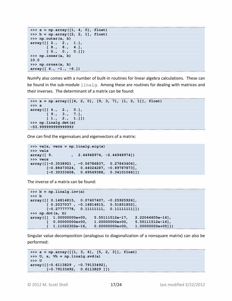
It is also possible to generate inner, outer, and cross products of matrices and vectors. For

vectors, note that the inner product is equivalent to the dot product:


>>> a = np.array([1, 4, 0], float) >>> b = np.array([2, 2, 1], float) >>> np.outer(a, b) array([[ 2., 2., 1.], [ 8., 8., 4.], [ 0., 0., 0.]]) >>> np.inner(a, b) 10.0 >>> np.cross(a, b) array([ 4., -1., -6.])

NumPy also comes with a number of built-in routines for linear algebra calculations. These can

be found in the sub-module linalg. Among these are routines for dealing with matrices and

their inverses. The determinant of a matrix can be found:

>>> a = np.array([[4, 2, 0], [9, 3, 7], [1, 2, 1]], float) >>> a array([[ 4., 2., 0.], [ 9., 3., 7.], [ 1., 2., 1.]]) >>> np.linalg.det(a) -53.999999999999993

One can find the eigenvalues and eigenvectors of a matrix:

>>> vals, vecs = np.linalg.eig(a) >>> vals array([ 9. , 2.44948974, -2.44948974]) >>> vecs array([[-0.3538921 , -0.56786837, 0.27843404], [-0.88473024, 0.44024287, -0.89787873], [-0.30333608, 0.69549388, 0.34101066]])

The inverse of a matrix can be found:

>>> b = np.linalg.inv(a) >>> b array([[ 0.14814815, 0.07407407, -0.25925926], [ 0.2037037 , -0.14814815, 0.51851852], [-0.27777778, 0.11111111, 0.11111111]]) >>> np.dot(a, b) array([[ 1.00000000e+00, 5.55111512e-17, 2.220 44605e-16], [ 0.00000000e+00, 1.00000000e+00, 5.551 11512e-16], [ 1.11022302e-16, 0.00000000e+00, 1.000 00000e+00]])

Singular value decomposition (analogous to diagonalization of a nonsquare matrix) can also be

performed:

>>> a = np.array([[1, 3, 4], [5, 2, 3]], float) >>> U, s, Vh = np.linalg.svd(a) >>> U array([[-0.6113829 , -0.79133492], [-0.79133492, 0.6113829 ]])


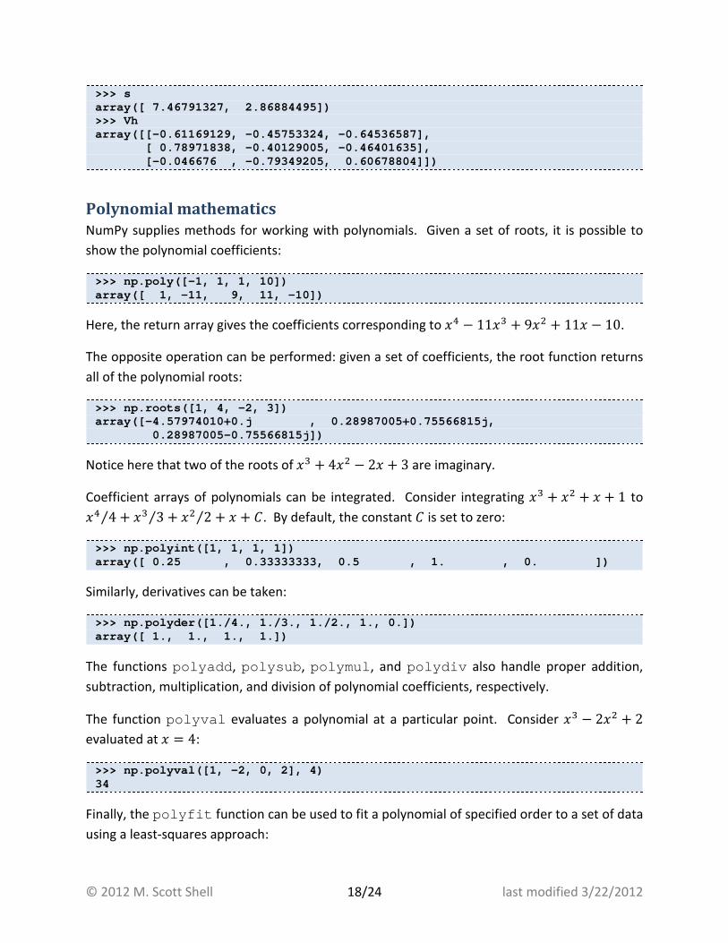
>>> s array([ 7.46791327, 2.86884495]) >>> Vh array([[-0.61169129, -0.45753324, -0.64536587], [ 0.78971838, -0.40129005, -0.46401635], [-0.046676 , -0.79349205, 0.60678804]])

Polynomial mathematics

NumPy supplies methods for working with polynomials. Given a set of roots, it is possible to

show the polynomial coefficients:

>>> np.poly([-1, 1, 1, 10]) array([ 1, -11, 9, 11, -10])

Here, the return array gives the coefficients corresponding to �� − 11�� + 9�� + 11� − 10.

The opposite operation can be performed: given a set of coefficients, the root function returns

all of the polynomial roots:

>>> np.roots([1, 4, -2, 3]) array([-4.57974010+0.j , 0.28987005+0.75566 815j, 0.28987005-0.75566815j])

Notice here that two of the roots of �� + 4�� − 2� + 3 are imaginary.

Coefficient arrays of polynomials can be integrated. Consider integrating �� + �� + � + 1 to

�� 4⁄ + �� 3⁄ + �� 2⁄ + � + �. By default, the constant � is set to zero:

>>> np.polyint([1, 1, 1, 1]) array([ 0.25 , 0.33333333, 0.5 , 1. , 0. ])

Similarly, derivatives can be taken:

>>> np.polyder([1./4., 1./3., 1./2., 1., 0.]) array([ 1., 1., 1., 1.])

The functions polyadd, polysub, polymul, and polydiv also handle proper addition,

subtraction, multiplication, and division of polynomial coefficients, respectively.

The function polyval evaluates a polynomial at a particular point. Consider �� − 2�� + 2

evaluated at � = 4:

>>> np.polyval([1, -2, 0, 2], 4) 34

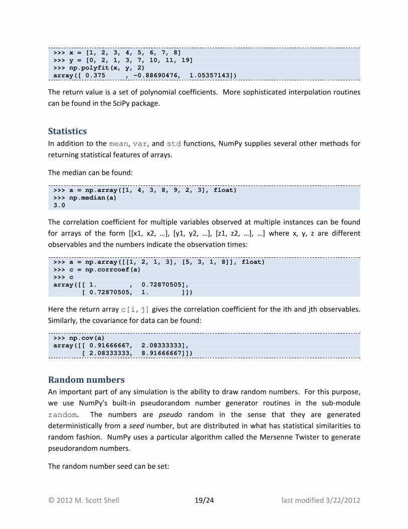
Finally, the polyfit function can be used to fit a polynomial of specified order to a set of data

using a least-squares approach:


>>> x = [1, 2, 3, 4, 5, 6, 7, 8] >>> y = [0, 2, 1, 3, 7, 10, 11, 19] >>> np.polyfit(x, y, 2) array([ 0.375 , -0.88690476, 1.05357143])

The return value is a set of polynomial coefficients. More sophisticated interpolation routines

can be found in the SciPy package.

Statistics

In addition to the mean, var, and std functions, NumPy supplies several other methods for

returning statistical features of arrays.

The median can be found:

>>> a = np.array([1, 4, 3, 8, 9, 2, 3], float) >>> np.median(a) 3.0

The correlation coefficient for multiple variables observed at multiple instances can be found

for arrays of the form [[x1, x2, …], [y1, y2, …], [z1, z2, …], …] where x, y, z are different

observables and the numbers indicate the observation times:

>>> a = np.array([[1, 2, 1, 3], [5, 3, 1, 8]], floa t) >>> c = np.corrcoef(a) >>> c array([[ 1. , 0.72870505], [ 0.72870505, 1. ]])

Here the return array c[i,j] gives the correlation coefficient for the ith and jth observables.

Similarly, the covariance for data can be found:

>>> np.cov(a) array([[ 0.91666667, 2.08333333], [ 2.08333333, 8.91666667]])

Random numbers

An important part of any simulation is the ability to draw random numbers. For this purpose,

we use NumPy's built-in pseudorandom number generator routines in the sub-module

random. The numbers are pseudo random in the sense that they are generated

deterministically from a seed number, but are distributed in what has statistical similarities to

random fashion. NumPy uses a particular algorithm called the Mersenne Twister to generate

pseudorandom numbers.

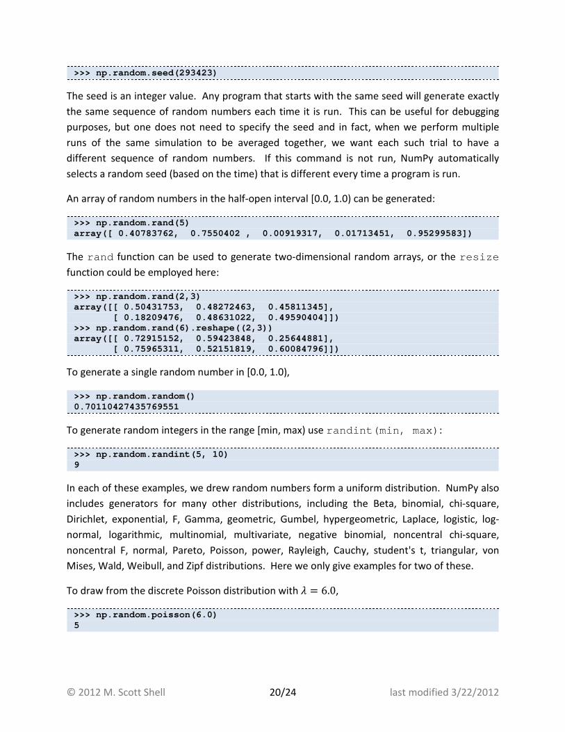
The random number seed can be set:


>>> np.random.seed(293423)

The seed is an integer value. Any program that starts with the same seed will generate exactly

the same sequence of random numbers each time it is run. This can be useful for debugging

purposes, but one does not need to specify the seed and in fact, when we perform multiple

runs of the same simulation to be averaged together, we want each such trial to have a

different sequence of random numbers. If this command is not run, NumPy automatically

selects a random seed (based on the time) that is different every time a program is run.

An array of random numbers in the half-open interval [0.0, 1.0) can be generated:

>>> np.random.rand(5) array([ 0.40783762, 0.7550402 , 0.00919317, 0.01 713451, 0.95299583])

The rand function can be used to generate two-dimensional random arrays, or the resize

function could be employed here:

>>> np.random.rand(2,3) array([[ 0.50431753, 0.48272463, 0.45811345], [ 0.18209476, 0.48631022, 0.49590404]]) >>> np.random.rand(6).reshape((2,3)) array([[ 0.72915152, 0.59423848, 0.25644881], [ 0.75965311, 0.52151819, 0.60084796]])

To generate a single random number in [0.0, 1.0),

>>> np.random.random() 0.70110427435769551

To generate random integers in the range [min, max) use randint(min, max):

>>> np.random.randint(5, 10) 9

In each of these examples, we drew random numbers form a uniform distribution. NumPy also

includes generators for many other distributions, including the Beta, binomial, chi-square,

Dirichlet, exponential, F, Gamma, geometric, Gumbel, hypergeometric, Laplace, logistic, log-

normal, logarithmic, multinomial, multivariate, negative binomial, noncentral chi-square,

noncentral F, normal, Pareto, Poisson, power, Rayleigh, Cauchy, student's t, triangular, von

Mises, Wald, Weibull, and Zipf distributions. Here we only give examples for two of these.

To draw from the discrete Poisson distribution with � = 6.0,

>>> np.random.poisson(6.0) 5


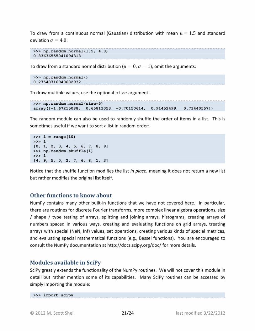
To draw from a continuous normal (Gaussian) distribution with mean � = 1.5 and standard

deviation � = 4.0:

>>> np.random.normal(1.5, 4.0) 0.83636555041094318

To draw from a standard normal distribution (� = 0, � = 1), omit the arguments:

>>> np.random.normal() 0.27548716940682932

To draw multiple values, use the optional size argument:

>>> np.random.normal(size=5) array([-1.67215088, 0.65813053, -0.70150614, 0.91 452499, 0.71440557])

The random module can also be used to randomly shuffle the order of items in a list. This is

sometimes useful if we want to sort a list in random order:

>>> l = range(10) >>> l [0, 1, 2, 3, 4, 5, 6, 7, 8, 9] >>> np.random.shuffle(l) >>> l [4, 9, 5, 0, 2, 7, 6, 8, 1, 3]

Notice that the shuffle function modifies the list in place, meaning it does not return a new list

but rather modifies the original list itself.

Other functions to know about

NumPy contains many other built-in functions that we have not covered here. In particular,

there are routines for discrete Fourier transforms, more complex linear algebra operations, size

/ shape / type testing of arrays, splitting and joining arrays, histograms, creating arrays of

numbers spaced in various ways, creating and evaluating functions on grid arrays, treating

arrays with special (NaN, Inf) values, set operations, creating various kinds of special matrices,

and evaluating special mathematical functions (e.g., Bessel functions). You are encouraged to

consult the NumPy documentation at http://docs.scipy.org/doc/ for more details.

Modules available in SciPy

SciPy greatly extends the functionality of the NumPy routines. We will not cover this module in

detail but rather mention some of its capabilities. Many SciPy routines can be accessed by

simply importing the module:

>>> import scipy


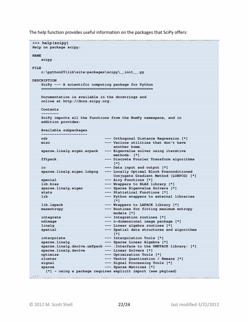
The help function provides useful information on the packages that SciPy offers:

>>> help(scipy) Help on package scipy: NAME scipy FILE c:\python25\lib\site-packages\scipy\__init__.py DESCRIPTION SciPy --- A scientific computing package for Py thon =============================================== ==== Documentation is available in the docstrings an d online at http://docs.scipy.org. Contents -------- SciPy imports all the functions from the NumPy namespace, and in addition provides: Available subpackages --------------------- odr --- Orthogonal Dis tance Regression [*] misc --- Various utilit ies that don't have another home. sparse.linalg.eigen.arpack --- Eigenvalue sol ver using iterative methods. [*] fftpack --- Discrete Fouri er Transform algorithms [*] io --- Data input and output [*] sparse.linalg.eigen.lobpcg --- Locally Optima l Block Preconditioned Conjugate Grad ient Method (LOBPCG) [*] special --- Airy Functions [*] lib.blas --- Wrappers to BL AS library [*] sparse.linalg.eigen --- Sparse Eigenva lue Solvers [*] stats --- Statistical Fu nctions [*] lib --- Python wrapper s to external libraries [*] lib.lapack --- Wrappers to LA PACK library [*] maxentropy --- Routines for f itting maximum entropy models [*] integrate --- Integration ro utines [*] ndimage --- n-dimensional image package [*] linalg --- Linear algebra routines [*] spatial --- Spatial data s tructures and algorithms [*] interpolate --- Interpolation Tools [*] sparse.linalg --- Sparse Linear Algebra [*] sparse.linalg.dsolve.umfpack --- :Interface to the UMFPACK library: [*] sparse.linalg.dsolve --- Linear Solvers [*] optimize --- Optimization T ools [*] cluster --- Vector Quantiz ation / Kmeans [*] signal --- Signal Process ing Tools [*] sparse --- Sparse Matrice s [*] [*] - using a package requires explicit impor t (see pkgload) ...


Notice that a number of sub-modules in SciPy require explicit import, as indicated by the star

notation above:

>>> import scipy >>> import scipy.interpolate

The functions in each module are well-documented in both the internal docstrings and at the

SciPy documentation website. Many of these functions provide instant access to common

numerical algorithms, and are very easy to implement. Thus, SciPy can save tremendous

amounts of time in scientific computing applications since it offers a library of pre-written, pre-

tested routines.

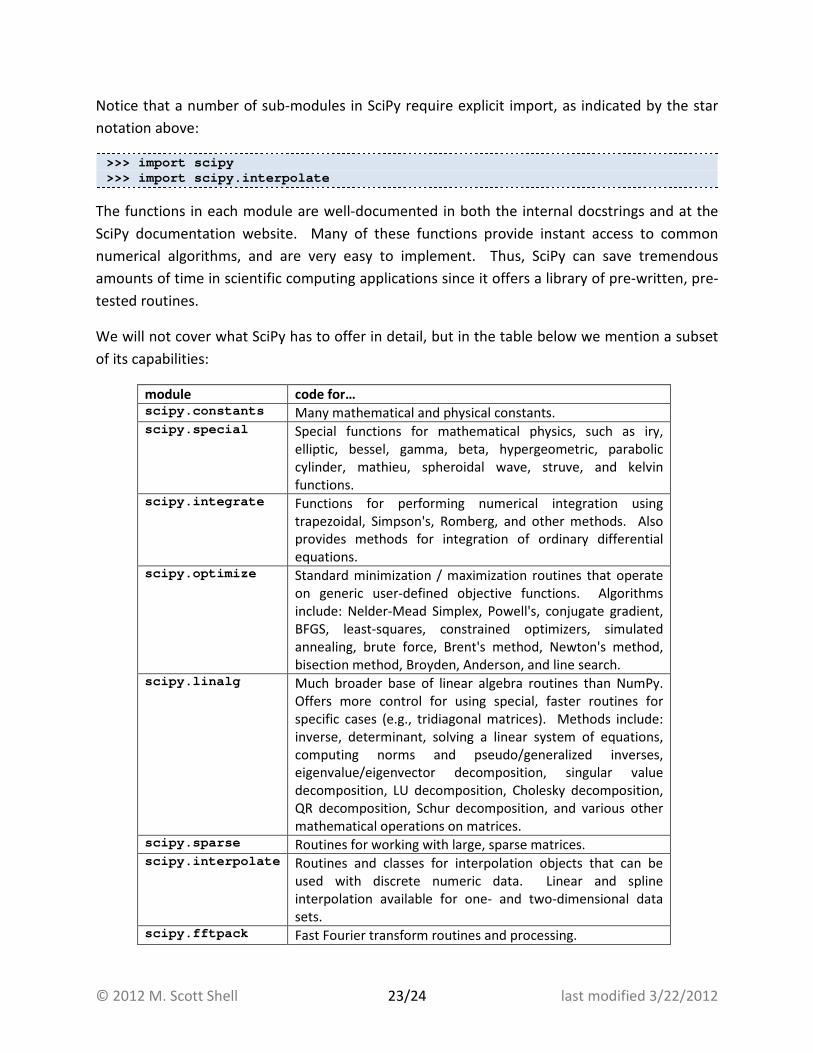
We will not cover what SciPy has to offer in detail, but in the table below we mention a subset

of its capabilities:

module code for…

scipy.constants Many mathematical and physical constants. scipy.special Special functions for mathematical physics, such as iry,

elliptic, bessel, gamma, beta, hypergeometric, parabolic

cylinder, mathieu, spheroidal wave, struve, and kelvin

functions. scipy.integrate Functions for performing numerical integration using

trapezoidal, Simpson's, Romberg, and other methods. Also

provides methods for integration of ordinary differential

equations. scipy.optimize Standard minimization / maximization routines that operate

on generic user-defined objective functions. Algorithms

include: Nelder-Mead Simplex, Powell's, conjugate gradient,

BFGS, least-squares, constrained optimizers, simulated

annealing, brute force, Brent's method, Newton's method,

bisection method, Broyden, Anderson, and line search. scipy.linalg Much broader base of linear algebra routines than NumPy.

Offers more control for using special, faster routines for

specific cases (e.g., tridiagonal matrices). Methods include:

inverse, determinant, solving a linear system of equations,

computing norms and pseudo/generalized inverses,

eigenvalue/eigenvector decomposition, singular value

decomposition, LU decomposition, Cholesky decomposition,

QR decomposition, Schur decomposition, and various other

mathematical operations on matrices. scipy.sparse Routines for working with large, sparse matrices. scipy.interpolate Routines and classes for interpolation objects that can be

used with discrete numeric data. Linear and spline

interpolation available for one- and two-dimensional data

sets. scipy.fftpack Fast Fourier transform routines and processing.


scipy.signal Signal processing routines, such as convolution, correlation,

finite fourier transforms, B-spline smoothing, filtering, etc. scipy.stats Huge library of various statistical distributions and statistical

functions for operating on sets of data.

A large community of developers continually builds new functionality into SciPy. A good rule of

thumb is: if you are thinking about implementing a numerical routine into your code, check the

SciPy documentation website first. Chances are, if it's a common task, someone will have

added it to SciPy.

an introduction to numpy and scipy -...

Documents