an introduction to mesh generation part iv : elliptic meshing

Elliptic Mesh Generation

An introduction to mesh generationPart IV : elliptic meshing

Jean-François Remacle

Department of Civil Engineering,Université catholique de Louvain, Belgium

Jean-François Remacle Mesh Generation


Curvilinear Meshes

Basic conceptA curvilinear mesh is build using a parametric spaceSponge analogyLet us consider the real coordonates (x,y) and a parametric space (u,v).

The transformation x = x(u,v) and y = y(u,v) has to be build.



Curvilinear Meshes

The transformation transforms a cartesian mesh in the parametric space intoa structured mesh in the real space with the following properties:

Two non intersecting lines in the parametric space do not cross in thereal space,The mesh adapts to the boundary of on the real space,The mesh has not to be orthogonal in the real space.



Curvilinear Meshes

The transformation transforms a cartesian mesh in the parametric space intoa structured mesh in the real space with the following properties:

Two non intersecting lines in the parametric space do not cross in thereal space,The mesh adapts to the boundary of on the real space,The mesh has not to be orthogonal in the real space.

The advantage of curvilinear meshes are numerous. They are usually highquality/very regular meshes. Yet, the sponge analogy cannot be appliedeasily to complex domains.



Transfinite Interpolation

Let us consider a simply connected 2D manifold that is bounded by 4curves ~ci(t), i = 1. . . ,4.We consider the four corners ~Pi,j that are the intersections if curves ~ciand ~cj.We look for a transformation that maps the unit square in theparametric space into the domain of interest.We suppose that curves ~c1 and ~c3 will be the mapping of the verticalsegments v = 0 and v = 1.We suppose that curves ~c2 and ~c4 will be the mapping of the horizontalsegments u = 0 and u = 1.




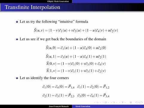
Let us try the following “intuitive” formula

~S(u,v) = (1−v)~c1(u)+v~c3(u)+(1−u)~c4(v)+u~c2(v)

Let us see if we get back the boundaries of the domain

~S(u,0) =~c1(u)+(1−u)~c4(0)+u~c2(0)

~S(u,1) =~c3(u)+(1−u)~c4(1)+u~c2(1)

~S(0,v) = (1−v)~c1(0)+v~c3(0)+~c4(v)

~S(1,v) = (1−v)~c1(1)+v~c3(1)+~c2(v)

Let us identify the four corners

~c1(0) =~c4(0) = ~P1,4 ~c1(1) =~c2(0) = ~P1,2

~c2(1) =~c3(1) = ~P2,3 ~c3(0) =~c4(1) = ~P3,4




Taking into account the corners

~S(u,0) =~c1(u)+(1−u)~P1,4 +u~P1,2 6=~c1(u)

~S(u,1) =~c3(u)+(1−u)~P3,4 +u~P2,3 6=~c3(u)

~S(0,v) = (1−v)~P1,4 +v~P3,4 +~c4(v) 6=~c4(v)

~S(1,v) = (1−v)~P1,2 +v~P2,3 +~c2(v) 6=~c2(v)

Let us try an alternative formula

~S(u,v) = (1−v)~c1(u)+v~c3(u)+(1−u)~c2(v)+u~c4(v)−[(1−u)(1−v)~P1,4 +uv~P2,3 +u(1−v)~P1,2 +(1−u)v~P3,4

].




~S(u,v) = (1−v)~c1(u)+v~c3(u)+(1−u)~c2(v)+u~c4(v)−[(1−u)(1−v)~P1,4 +uv~P2,3 +u(1−v)~P1,2 +(1−u)v~P3,4

].

Taking into account corners

~S(u,0) =~c1(u)+(1−u)~P1,4 +u~P1,2 −(1−u)~P1,4 −u~P1,2 =~c1(u)

~S(u,1) =~c3(u)+(1−u)~P3,4 +u~P2,3 −(1−u)~P3,4 −u~P2,3 =~c3(u)

~S(0,v) = (1−v)~P1,4 +v~P3,4 +~c4(v)−(1−v)~P1,4 −v~P3,4 =~c4(v)

~S(1,v) = (1−v)~P1,2 +v~P2,3 +~c2(v)−(1−v)~P1,2 −v~P2,3 =~c2(v)

This formula is correct, it is called the transfinite interpolation formula.




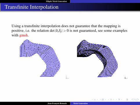
Using a transfinite interpolation does not guarantee that the mapping ispositive, i.e. the relation det |∂iSj| > 0 is not guaranteed, see some exampleswith gmsh.




Transfinite interpolation exists for 3-sides shapes,

~S(u,v) = u~c2(v)+(1−v)~c1(u)+v~c3(v)−[u(1−v)~P1,2 +uv~P2,3

].

Transfinite interpolation exists for 3D shapes.



Elliptic meshes

It is not always simple to devise an explicit formula for the meshmapping,With the transfinite interpolation, mesh lines may cross each others,leading to a wrong meshPDE based mesh have been developped in order to avoid thosedifficultiesTwo kind of approaches are possible, using either an hyperbolic PDE,or using an elliptic PDE. This last approach is now studied.



Elliptic meshes : Thermal Analogy

Let us consider the same 4-sided domain as the one we used fortransfinite meshing,We build mesh lines using a thermal analogy : mesh lines aresuperimposed with the isolines of temperature.Steady state heat equation has to be solved.Two sides of the domain are adiabatical and a constant temperature isimposed on the two other sides.

!

" "

!

©

τ

∇2τ = 0

∇2η = 0

©




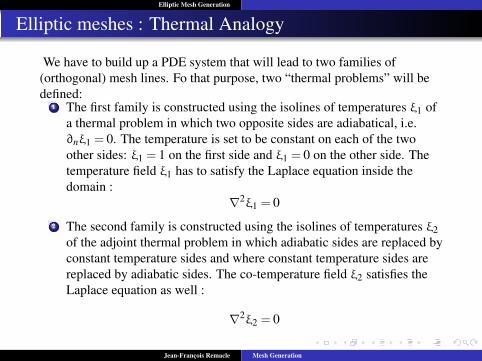
We have to build up a PDE system that will lead to two families of(orthogonal) mesh lines. Fo that purpose, two “thermal problems” will bedefined:

1 The first family is constructed using the isolines of temperatures ξ1 ofa thermal problem in which two opposite sides are adiabatical, i.e.∂nξ1 = 0. The temperature is set to be constant on each of the twoother sides: ξ1 = 1 on the first side and ξ1 = 0 on the other side. Thetemperature field ξ1 has to satisfy the Laplace equation inside thedomain :

∇2ξ1 = 0

2 The second family is constructed using the isolines of temperatures ξ2of the adjoint thermal problem in which adiabatic sides are replaced byconstant temperature sides and where constant temperature sides arereplaced by adiabatic sides. The co-temperature field ξ2 satisfies theLaplace equation as well :

∇2ξ2 = 0




The two families of mesh lines will have the right properties, thanks to theproperties of the solutions of the Laplace equation:

The maximum principle : any solution of the Laplace equation has itsmaximum on the boundaries (no local maxima is allowed),

→ The solution is unique,The solution belongs to H1, it is smooth,

→ Iso-contours cannot intersect,→ Iso-contours stay inside the domain (obvious for a PDE, not for a

general mapping),



Elliptic meshes : Formulation

The resulting “mesh equations” are two boundary value problems. Wehave to find ξ1 and ξ2 solution of

∇2ξi = 0 , i = 1,2.

boundary conditions are

Boundary ξ1 ξ2~c1 ξ1(x,y) = 0 ∂nξ2(x,y) = 0~c2 ∂nξ1(x,y) = 0 ξ2(x,y) = 0~c3 ξ1(x,y) = 1 ∂nξ2(x,y) = 0~c4 ∂nξ1(x,y) = 0 ξ2(x,y) = 1




Problem : the equations have to be solved in the real space.Disappointingly, solving such PDE requires... a mesh !




This issue is addresded by the inversion of variables x and y and ξ1 andξ2,The problem is solved in the space of temperatures ξ1 and ξ2 and theunknowns are the positions of the mesh in the real space x and y,For a pair of temperatures (ξ1,ξ2), we look the point (x,y) in thephysical space where this temperature occurs.Because of the properties of the Laplace operator, the exist such apoint (x,y) for any pair (ξ1,ξ2) for which 0 6 ξ1 6 1 and for which0 6 ξ2 6 1This is equivalent to the following change of variables

x = x1 = x1(ξ1,ξ2) and y = x2 = x2(ξ1,ξ2)




We use the chain derivative rule to compute

∂

∂xj=

2∑j=1

∂

∂ξj

∂ξj

∂xiand

∂2

∂xi∂xk=

2∑j=1

2∑l=1

∂2

∂ξjξl

∂ξl

∂xk

∂ξj

∂xi

In expanded form

∂2

∂x21

=∂2

∂ξ21

(∂ξ1

∂x1

)2+2

∂2

∂ξ1∂ξ2

(∂ξ1

∂x1

∂ξ2

∂x1

)+

∂2

∂ξ22

(∂ξ2

∂x1

)2.

∂2

∂x22

=∂2

∂ξ21

(∂ξ1

∂x2

)2+2

∂2

∂ξ1∂ξ2

(∂ξ1

∂x2

∂ξ2

∂x2

)+

∂2

∂ξ22

(∂ξ2

∂x2

)2.




The Laplace operator is written as

∇2 =∂2

∂ξ21

((∂ξ1

∂x1

)2+

(∂ξ1

∂x2

)2)

+2∂2

∂ξ1∂ξ2

(∂ξ1

∂x1

∂ξ2

∂x1+

∂ξ1

∂x2

∂ξ2

∂x2

)+

+∂2

∂ξ22

((∂ξ2

∂x1

)2+

(∂ξ2

∂x2

)2)

.

Therefore, in 2D, the PDE’s that have to be solved can be written as

α

∂2x1∂ξ2

1∂2x2∂ξ2

1

+2β

∂2x1∂ξ1∂ξ2

∂2x2∂ξ1∂ξ2

+γ

∂2x1∂ξ2

2∂2x2∂ξ2

2

= 0.

with

α =

(∂ξ1

∂x1

)2+

(∂ξ1

∂x2

)2, β =

∂ξ1

∂x1

∂ξ2

∂x1+

∂ξ1

∂x2

∂ξ2

∂x2, γ =

(∂ξ2

∂x1

)2+

(∂ξ2

∂x2

)2




Note that

α = J2

[(∂x1

∂ξ1

)2+

(∂x1

∂ξ2

)2]

=

(∂ξ1

∂x1

)2+

(∂ξ1

∂x2

)2,

β = −J2[

∂x1

∂ξ1

∂x2

∂ξ1+

∂x1

∂ξ2

∂x2

∂ξ2

]=

∂ξ1

∂x1

∂ξ2

∂x1+

∂ξ1

∂x2

∂ξ2

∂x2,

γ = J2

[(∂x2

∂ξ1

)2+

(∂x2

∂ξ2

)2]

=

(∂ξ2

∂x1

)2+

(∂ξ2

∂x2

)2,

withJ = det[∂ξjxi]




The equations that have to be solved for the mesh problem are coupled andnon-linear! They can only be solved using numerical methods. There existsseveral techniques to solve such systems. We are not going to detail all themethods that are available (this is could be the subject of another course).We are going to illustrate some basic principles. Two items will be detailedhere

The numerical discretization of the mesh equations in the parametricspace (ξ1,ξ2),Their resolution.




We assume that the “mesh” in the parametric space is a m×n finitedifference mesh. The mesh is uniform in the sense that the spacings ∆τ and∆η in both directions are constant.

m n τ η

i j

τi = (i − 1)∆τ 1 ≤ i ≤ m

ηj = (j − 1)∆η 1 ≤ j ≤ n

∆τ ∆η

∆τ = (τm − τ1)/(m − 1)

∆η = (ηn − η1)/(n − 1)

(i, j)

fi,j = f(τi, ηj)

©

∂f

∂τ≈ fi+1,j − fi−1,j

2∆τ∂f

∂η≈ fi,j+1 − fi,j−1

2∆η

∂2f

∂τ2≈ fi+1,j − 2fi,j + fi−1,j

∆τ2

∂2f

∂η2≈ fi,j+1 − 2fi,j + fi,j−1

∆η2

∂2f

∂τ∂η≈ fi+1,j+1 − fi+1,j−1 − fi−1,j+1 + fi−1,j−1

4∆τ∆η

L = α∂2

∂η2+ 2β

∂2

∂η∂τ+ γ

∂2

∂τ2

(i, j)x y

α′ [xi+1,j − 2xi,j + xi−1,j ] + γ′ [xi,j+1 − 2xi,j + xi,j−1]

−2β′ [xi+1,j+1 − xi−1,j+1 − xi+1,j−1 + xi−1,j−1] = 0

α′ [yi+1,j − 2yi,j + yi−1,j] + γ′ [yi,j+1 − 2yi,j + yi,j−1]

−2β′ [yi+1,j+1 − yi−1,j+1 − yi+1,j−1 + yi−1,j−1] = 0

©




We recall the mesh equations

α

∂2x1∂ξ2

1∂2x2∂ξ2

1

+2β

∂2x1∂ξ1∂ξ2

∂2x2∂ξ1∂ξ2

+γ

∂2x1∂ξ2

2∂2x2∂ξ2

2

= 0.

Their discrete version can be written, for any vertex (i, j) of the mesh in theparametric space, as

m n τ η

i j

τi = (i − 1)∆τ 1 ≤ i ≤ m

ηj = (j − 1)∆η 1 ≤ j ≤ n

∆τ ∆η

∆τ = (τm − τ1)/(m − 1)

∆η = (ηn − η1)/(n − 1)

(i, j)

fi,j = f(τi, ηj)

©

∂f

∂τ≈ fi+1,j − fi−1,j

2∆τ∂f

∂η≈ fi,j+1 − fi,j−1

2∆η

∂2f

∂τ2≈ fi+1,j − 2fi,j + fi−1,j

∆τ2

∂2f

∂η2≈ fi,j+1 − 2fi,j + fi,j−1

∆η2

∂2f

∂τ∂η≈ fi+1,j+1 − fi+1,j−1 − fi−1,j+1 + fi−1,j−1

4∆τ∆η

L = α∂2

∂η2+ 2β

∂2

∂η∂τ+ γ

∂2

∂τ2

(i, j)x y

α′ [xi+1,j − 2xi,j + xi−1,j ] + γ′ [xi,j+1 − 2xi,j + xi,j−1]

−2β′ [xi+1,j+1 − xi−1,j+1 − xi+1,j−1 + xi−1,j−1] = 0

α′ [yi+1,j − 2yi,j + yi−1,j] + γ′ [yi,j+1 − 2yi,j + yi,j−1]

−2β′ [yi+1,j+1 − yi−1,j+1 − yi+1,j−1 + yi−1,j−1] = 0

©Jean-François Remacle Mesh Generation


Elliptic meshes : Resolution

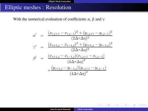
With the numerical evaluation of coefficients α, β and γ

α′ =(xi,j+1 − xi,j−1)2 + (yi,j+1 − yi,j−1)2

(2∆τ∆η)2

γ′ =(xi+1,j − xi−1,j)2 + (yi+1,j − yi−1,j)2

(2∆τ∆η)2

β′ =(xi+1,j − xi−1,j)(xi,j+1 − xi,j−1)

(4∆τ∆η)2

+(yi+1,j − yi−1,j)(yi,j+1 − yi,j−1)

(4∆τ∆η)2

α′ γ′ β′ x

y

©

i i+1

j

j−1

j+1

i−1

valeurs à l’étape n + 1

valeurs à l’étape n

valeur courante

(i, j)

©




Applying the formulation to the m×n nodes of the finite difference mesh,we obtain a coupled system of non linear equations. In fact, α ′, β ′ and γ ′

are all functions of the unknowns, i.e. the position of the nodes in the realspace. Several methods are available for solving such a system. They can beclassified in two categories:

1 direct methods,2 iterative methods.

The choice of the method is essentially based on the following criterionThe CPU time cost and the memory cost,The ability of the method to converge to the solution,The relative ease of programming !




Direct methods are not the choice that is usually made for building ellipticmeshes. Direct methods have the advantage of ensuring the convergence ina finite number of step (yet this not true for non-linear systems). Theirprincipal drawback is their memory signature and their (relative)complexity.Iterative methods have the following advantages:

1 They are usually easier to code,2 They are well adapted to structured grids,

The following “smoothers” are often used for building elliptic meshesPoint Jacobi iteration,Block Jacobi iteration (the block may be a line or a column of nodes),ADI’s, i.e. alternated direction implicit !



Elliptic meshes : Point Jacobi Iteration

We look for the values of the variables x and y, noted x− and y− at node(i, j) verifying x y (i, j) x− y−

α′ [xi+1,j − 2x−i,j + x+

i−1,j

]+ γ′ [xi,j+1 − 2x−

i,j + x+i,j−1

]

−2β′ [xi+1,j+1 − xi−1,j+1 − x+i+1,j−1 + x+

i−1,j−1

]= 0

α′ [yi+1,j − 2y−i,j + y+i−1,j

]+ γ′ [yi,j+1 − 2y−i,j + y+

i,j−1

]

−2β′ [yi+1,j+1 − yi−1,j+1 − y+i+1,j−1 + y+

i−1,j−1

]= 0

x y n x+ y+

n + 1α′ γ′ β′ x y

x y (x− − x) (y− − y)ω

x+ = x + ω(x− − x

)

y+ = y + ω(y− − y

)

x−i,j = xi,j + Cxi, j/ω

y−i,j = yi,j + Cyi, j/ω

Cxi, j = x+i,j − xi,j

Cyi, j = y+i,j − yi,j

©

2(α′ + γ′)ω

Cxi, j = Rxi, j + α′Cxi − 1, j

−β′(Cxi − 1, j − 1 − Cxi + 1, j − 1) + γ′Cxi, j − 12(α′ + γ′)

ωCyi, j = Ryi, j + α′Cyi − 1, j

−β′(Cyi − 1, j − 1 − Cyi + 1, j − 1) + γ′Cyi, j − 1

Rxi, j = α′ [xi+1,j − 2xi,j + xi−1,j] + γ′ [xi,j+1 − 2xi,j + xi,j−1]

−2β′ [xi+1,j+1 − xi−1,j+1 − xi+1,j−1 + xi−1,j−1]

Ryi, j = α′ [yi+1,j − 2yi,j + yi−1,j ] + γ′ [yi,j+1 − 2yi,j + yi,j−1]

−2β′ [yi+1,j+1 − yi−1,j+1 − yi+1,j−1 + yi−1,j−1]

!

" "

#

$

$

"

#

#$

!

!

!!

% %

%

& '

&

'

" "

©

Here, x− and y− are for the values of x and y at the previous sweep and x−

and y− are the values at the present sweep. The linearization of thecoefficients consist in using previous values of x and y in α ′, β ′ and γ ′.



Elliptic meshes : Over relaxation

We know that x and y are updated by doing

x = x+(x− −x) and y = y+(y− −y).

Over relaxing the system consist in doing

x+ = x+ω(x− −x) and y+ = y+ω(y− −y).

with ω > 1. Current values are computed as

x−i,j = xi,j +Cxi, j/ω and y−

i,j = yi,j +Cyi, j/ω.

with the corrections

Cxi, j = x+i,j −xi,j and Cyi, j = y+

i,j −yi,j.



Elliptic meshes : Over relaxation

Replacing in the discrete form of the equations, we obtainx y (i, j) x− y−

α′ [xi+1,j − 2x−i,j + x+

i−1,j

]+ γ′ [xi,j+1 − 2x−

i,j + x+i,j−1

]

−2β′ [xi+1,j+1 − xi−1,j+1 − x+i+1,j−1 + x+

i−1,j−1

]= 0

α′ [yi+1,j − 2y−i,j + y+i−1,j

]+ γ′ [yi,j+1 − 2y−i,j + y+

i,j−1

]

−2β′ [yi+1,j+1 − yi−1,j+1 − y+i+1,j−1 + y+

i−1,j−1

]= 0

x y n x+ y+

n + 1α′ γ′ β′ x y

x y (x− − x) (y− − y)ω

x+ = x + ω(x− − x

)

y+ = y + ω(y− − y

)





©

2(α′ + γ′)ω




−β′(Cyi − 1, j − 1 − Cyi + 1, j − 1) + γ′Cyi, j − 1


−2β′ [xi+1,j+1 − xi−1,j+1 − xi+1,j−1 + xi−1,j−1]


−2β′ [yi+1,j+1 − yi−1,j+1 − yi+1,j−1 + yi−1,j−1]

!

" "

#

$

$

"

#

#$

!

!

!!

% %

%

& '

&

'

" "

©

with the residuals

x y (i, j) x− y−

α′ [xi+1,j − 2x−i,j + x+

i−1,j

]+ γ′ [xi,j+1 − 2x−

i,j + x+i,j−1

]

−2β′ [xi+1,j+1 − xi−1,j+1 − x+i+1,j−1 + x+

i−1,j−1

]= 0

α′ [yi+1,j − 2y−i,j + y+i−1,j

]+ γ′ [yi,j+1 − 2y−i,j + y+

i,j−1

]

−2β′ [yi+1,j+1 − yi−1,j+1 − y+i+1,j−1 + y+

i−1,j−1

]= 0

x y n x+ y+

n + 1α′ γ′ β′ x y

x y (x− − x) (y− − y)ω

x+ = x + ω(x− − x

)

y+ = y + ω(y− − y

)





©

2(α′ + γ′)ω




−β′(Cyi − 1, j − 1 − Cyi + 1, j − 1) + γ′Cyi, j − 1


−2β′ [xi+1,j+1 − xi−1,j+1 − xi+1,j−1 + xi−1,j−1]


−2β′ [yi+1,j+1 − yi−1,j+1 − yi+1,j−1 + yi−1,j−1]

!

" "

#

$

$

"

#

#$

!

!

!!

% %

%

& '

&

'

" "

©



Elliptic meshes : Boundary conditions

We do not want to move the boundary nodes. The way to implement it isvery simple : do not apply any corrections to those nodes

Cxi, j Cyi, j

Cx1, j = Cxm, j = 0

Cy1, j = Cym, j = 0

x y (i, j)

τ η

m n

∆η ∆τ

©

valeurs courantes



j+1

i-1 i i+1

j

j-1

α′ [x−i+1,j − 2x−

i,j + x−i−1,j

]+ γ′ [xi,j+1 − 2x−

i,j + x+i,j−1

]

−2β′ [xi+1,j+1 − xi−1,j+1 − x+i+1,j−1 + x+

i−1,j−1

]= 0

α′ [y−i+1,j − 2y−i,j + y−i−1,j

]+ γ′ [yi,j+1 − 2y−i,j + y+

i,j−1

]

−2β′ [yi+1,j+1 − yi−1,j+1 − y+i+1,j−1 + y+

i−1,j−1

]= 0

©

Those are Dirichlet boundary conditions.



Elliptic meshes : Example

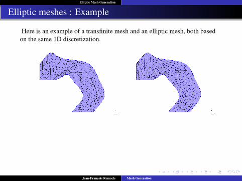
Here is an example of a transfinite mesh and an elliptic mesh, both basedon the same 1D discretization.



Elliptic meshes : Line Jacobi Iteration

Iterative process can be accelerated using a more implicit method. Wecound compute one line at a time

Cxi, j Cyi, j

Cx1, j = Cxm, j = 0

Cy1, j = Cym, j = 0

x y (i, j)

τ η

m n

∆η ∆τ

©

valeurs courantes



j+1

i-1 i i+1

j

j-1

α′ [x−i+1,j − 2x−

i,j + x−i−1,j

]+ γ′ [xi,j+1 − 2x−

i,j + x+i,j−1

]

−2β′ [xi+1,j+1 − xi−1,j+1 − x+i+1,j−1 + x+

i−1,j−1

]= 0

α′ [y−i+1,j − 2y−i,j + y−i−1,j

]+ γ′ [yi,j+1 − 2y−i,j + y+

i,j−1

]

−2β′ [yi+1,j+1 − yi−1,j+1 − y+i+1,j−1 + y+

i−1,j−1

]= 0

©

The resulting system is tridiagonal and ad hoc linear solvers can be used foraccelerating the process.



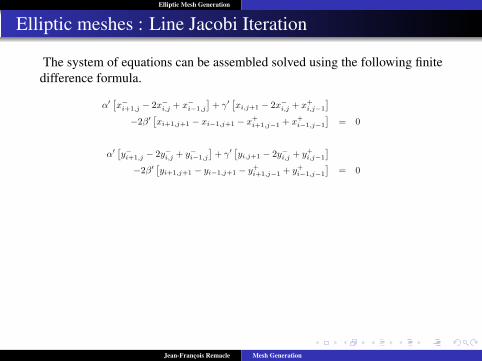
Elliptic meshes : Line Jacobi Iteration

The system of equations can be assembled solved using the following finitedifference formula.

Cxi, j Cyi, j

Cx1, j = Cxm, j = 0

Cy1, j = Cym, j = 0

x y (i, j)

τ η

m n

∆η ∆τ

©

valeurs courantes



j+1

i-1 i i+1

j

j-1

α′ [x−i+1,j − 2x−

i,j + x−i−1,j

]+ γ′ [xi,j+1 − 2x−

i,j + x+i,j−1

]

−2β′ [xi+1,j+1 − xi−1,j+1 − x+i+1,j−1 + x+

i−1,j−1

]= 0

α′ [y−i+1,j − 2y−i,j + y−i−1,j

]+ γ′ [yi,j+1 − 2y−i,j + y+

i,j−1

]

−2β′ [yi+1,j+1 − yi−1,j+1 − y+i+1,j−1 + y+

i−1,j−1

]= 0

©


an introduction to mesh generation part iv : elliptic meshing

Documents