An introduction to mathematical modeling

of signal transduction and gene control networks

Hans G. Othmer

Department of Mathematics

University of Minnesota

Minneapolis, MN

Overview

First Lecture: An introduction to mathematical modeling of signal transduction andgene control networks

• Examples of signal transduction, metabolic and gene control networks

• What is it we want to understand?

• The mathematical description of chemical reactions

• Analytical and computational techniques

Second lecture: Analysis of a model of signal transduction and motor control

• Signal transduction in bacteria

– The basic input-output behavior

– Response to steps and slow ramps

– The gain in the signal transduction pathway

– The bacterial motor

– Monte Carlo results

Third lecture: Analysis of a model for Drosophila melanogastersegment polarity genes

• Background on Drosophila development

• The basic facts about segment polarity genes

• Description of the Boolean representation

• Analysis of wild-type and heat-shock behavior

• Expression patterns in mutants

• A two-step model

Biochemical networks

• Signal transduction networks: The pathways and the molecular components, such as

kinases, G-proteins, sencond messengers, ..., involved in transducing a signal from one

location to another. Frequently used in the context of transduction of extra- into

intracellular signals.

• Metabolic networks: The pathways and the molecular components (metabolites,

enzymes, control factors) involved in the biosynthesis of new components, the conversion

of molecular ‘foodstuffs’ into energy, etc. One of the most important examples is the

glycolytic pathway, which converts sugars into energy-storing molecules such as ATP.

• Gene expression networks:The pathways and components, such as genes, polymerases,

transcription factors, etc., that are involved in gene expression, mRNA translation, etc.

An early view of signal transduction

To understand, next, how external objects that strike

the sense organs can incite [the machine] to move its

members in a thousand different ways: think that

(a) the filaments (I have already often told you that

these come from the innermost part of the brain and

compose the marrow of the nerves) are so arranged

that they can very easily be moved by the objects of

that sense and that

(b) when they are moved, with however little force,

they simultaneously pull the parts of the brain from

which they come, and by this means open the en-

trances to certain pores in the internal surface of the

brain ..

Thus if fire A is near foot B, the particles of this fire

have force enough to displace the area of skin they

touch; and thus pulling the little thread (cc) which

you see attached there, they simultaneously open the

entrance to the pore (de) where this thread termi-

nates; just as, pulling on one end of a cord, one si-

multaneously rings a bell which hangs on the oppo-

site end.

R. Descartes -De Homine

A global view of signal transduction

Lipid-soluble molecules can

pass through the cell mem-

brane, but most signals are

proteins or peptides and these

require more machinery ...

Y

Nucleus

Receptor

Cell

factorSoluble

Ligand

Receptors can transduce signals in a variety of ways

Receptor phosphorylation and G-protein activation: two majortransduction pathways

The G-protein motif

Some of the functions of G proteins

One mode involving phosphorylation: the RTK pathway

Downstream activation via RTKs

A Ras-mediated pathway

The signal transduction pathway in E. coli

+CH3R

ATP ADPP~

flagellarmotor

Z

Y

PY

~

PiB

B~P

Pi

CW-CH3

ATP

WA

MCPs

WA

+ATT

-ATT

MCPs

Metabolic networks

• Metabolism : The cellular process by which organic molecules are synthesized or

degraded, usually via enzyme-catalyzed reactions

• The interconnected components and reactions form a network, called themetabolicnetwork

E B

C

D

AE

P2

P

P

: A B

D

C

3

A

: A

P

P

P

C

4

5

6

E1 :

:

: C

D

: B1

2

3

E2

E3

E4

E5 E1 E6

E6E5

E4

Rather than viewing reactions in isolation, as on the left, we should begin thinking about the

underlying structure of the network, as well as the individual reactions, as on the right!

The glycolytic reactions

Glycolysis: Thelysis or split-

ting of glucose

Stage 2

Stage 1

molecules

Glycolysis

Stage 3Production of NADH

and ATP

Breakdown of complex

Gene control networks, development, and the French flag problem

The map from egg to adult in Drosophila melanogaster

The general structure of the gene network in Drosophila

The details of the segment polarity gene network

The general structure of signal transduction cascades

1. General scheme

Outside

Inside

Signal Transduction

Internal Response

Signal Propagation

External Signal External Signal

Signal Detection

55555555555555555555555555555555555555555555555555555555

55555555555555555555555555555555555555555555555555555555

Amplification of signals

Adaptation to constant signals

A single step change in the signal produces a single response and a return to the basal level of

activity, while a sequence of steps produces a sequence of responses.

Thus the system both adapts AND maintains sensitivity to further changes in the stimulus.

The role of adaptation in the visual system

What is it we want to understand about these networks?

• How do we describe their dynamical behavior? Do we use

1. a continuous state space and deterministic descriptions via ODE’s,

2. a Boolean representation of ON/OFF states and logical functions that determine the

dynamics, or

3. a stochastic description, in which we follow individual molecules.

How do we decide which is the appropriate choice?

• What are the ‘attractors’ in the dynamics? Are they steady states or fixed points, periodic

attractors, or are they more complicated?

• How do we define and then compute measures of amplification, sensitivity and gain?

• How sensitive is the behavior to variations in the parameters? In the structure of the

network itself ? From a dynamical systems point of view this might be viewed as a

question of ‘structural stability’; another way of phrasing this is to ask whether certain

features of the dynamics are robust.

What are the big questions about these networks?

• Why have the networks evolved to their present form? To what extent do the physics and

chemistry influence the structure of the networks? Said otherwise, if one wants to

synthesize Z from A, how many distinct (nontrivial) paths are there? The answer bears

on the inverse problem of inferring the network from expression patterns. Are there

design principles and evolutionary approaches that can help us understand the observed

structure?

• Many signal transduction systems adapt to constant signals but retain the ability to

respond to further changes. What structure in a dynamical system guarantees this

characteristic?

• Can we give a useful precise definition of robustness? How do we determine when

‘parametric robustness’ suffices and when ‘redundancy’ is necessary? Should we expect

robustness at the individual level, or can population-level feedbacks correct

individual-level variances in response to signals?

Two views on complex networks .......

”When the number of factors coming into play in a phenomenological complex is too large,

scientific method in most cases fails. One need only think of the weather, in which case the

prediction even for a few days ahead is impossible. Nevertheless, none doubts that we are

confronted with a causal connection whose causal components are in the main known to us.

Occurrences in this domain are beyond the reach of exact prediction because of the variety of

factors in operation, not because of any lack of order in nature.”

Albert Einstein

”Though signalling pathways are often drawn as simple linear chains of events, they are

rarely that simple. Frequently there is feedback, cross-talk between pathways and enough

branching to make one want to change to a less complicated field of biology.

In order to fully understand these pathways, we need a convenient and powerful model to

complement the experimental research. Though there have been relatively few attempts to

model signalling pathways using computers, it seems likely that this will very soon become a

major area of study.”

J. Michael Bishop, Science 267:1617

The mathematical description of chemical reaction networks

• The stochiometryof a chemical reaction denotes the molar ratios in which molecules

are converted into products in that reaction.

A + 2 B C

1 2 1

BA

11

k k

Rate = kA Rate = kAB2MAK:

Here, and unless specified otherwise later, we consider only mass action kinetics

(MAK ), which means that the rates are monomials in the concentrations, raised to the

power given by the stoichiometry, of the components that react together.

• Thestochiometric matrixν = (νij) provides a mathematical encoding of the

stoichiometry and topology of a reaction network

21P

A

P B

D

C

reactions

1 0 00 1 0 00 0 1 10 0 1 0

−1 −1−1

−1

00

00

P4

P5

P6

P3 −1 = ν reactants

The mathematical description of chemical reaction networks ...

Define the concentration and rate vectors

c =

c1

c2...

cn

P (c) =

P1(c)

P2(c)...

Pn(c)

Then the concentration evolves in time according the differential equation

dc

dt= νP (c)

(1)c(0) = c0

c

c

c

2

1

3

Reaction invariants

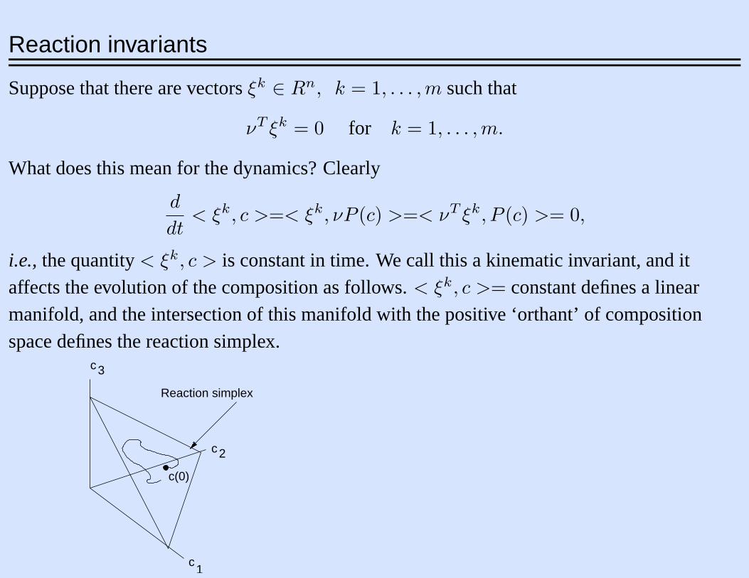
Suppose that there are vectorsξk ∈ Rn, k = 1, . . . ,m such that

νT ξk = 0 for k = 1, . . . ,m.

What does this mean for the dynamics? Clearly

d

dt< ξk, c >=< ξk, νP (c) >=< νT ξk, P (c) >= 0,

i.e., the quantity< ξk, c > is constant in time. We call this a kinematic invariant, and itaffects the evolution of the composition as follows.< ξk, c >= constant defines a linearmanifold, and the intersection of this manifold with the positive ‘orthant’ of compositionspace defines the reaction simplex.

c

c

c3

2

1

Reaction simplex

c(0)

Remark: Note thatνT has a nontrivial

null space if the number of species ex-

ceeds the number of reactions.

Enzyme-catalyzed reactions

LetE denote an enzyme, letS denote the substrate, letES denote the complex formed

whenS binds toE, and letP denote the product

E + S ES E + Pk k1 2

k−1

Herec = (E,S,ES, P )T and

ν =

−1 1 1

−1 1 0

1 −1 −1

0 0 1

The rank ofν is 2 and therefore dimN (νT ) = 2, so there are two kinematic invariants. We

can choose these asξ1 = (1, 0, 1, 0)T andξ2 = (0, 1, 1, 1)T . Thus the reaction simplex is

two-dimensional. How could we have predicted thisa priori?

Exercise: Determine how the reaction invariants reflect the conservation of atomic species in

the reaction

H2 +O−→←− H2O.

A Cartoon Model of Excitation and Adaptation

Excitation

Change

Adaptation

ResponseSignal

dy1

dτ=

S(τ)− (y1 + y2)τE

dy2

dτ=

S(τ)− y2

τA

For example,S(t) could be proportional to the fraction of receptors occupied.

y1 =S0τAτA + τE

(e−τ/τA − e−τ/τE )

y2 = S0(1− e−τ/τA)

1y

y2(a)

1S(τ) = 0 S(τ) = S

1y

y2(b)

S(τ) = 0 S(τ) = S1 S(τ) = S2

If τE << τA, then forτ >> τE, y1 relaxes to

y1 ∼ S0e−τ/τA ≡ S0 − y2(τ) = τAy2.

u ≡ y2 satisfies

du

dt+

1τAu =

1τA

dS

dt

Adaptation, Sensitivity and Gain

dx

dt= f(x, S(t))

Response

R = G(x(t)).

At steady state supposex = X(S); then adaptation requires that

dRdS

=∑ ∂G

∂xi

∂xi∂S

= 〈∇xG(X(S)), (Dxf)−1(X(S), S)DSf(X(S), S)〉 = 0

Definitions of gain and sensitivity

g0 ≡dRdS

=∑ ∂G

∂xi

∂xi∂S

gLS ≡dRd lnS

= Sg0

gLR ≡d lnRdS

=1Rg0 gLL ≡

d lnRd lnS

=S

Rg0

Thus the steady-state gain vanishes in a system that adapts perfectly!

Sensitivity of transient solutions

∂x

∂S= Φ(t, 0)

∂x

∂S(0) +

∫ t

0

Φ(t, τ)DSf(x(τ), S(τ))dτ

g = max[0,∞)

g(t)

Reported bacterial gains range from g =∼ 6 to g =∼ 55

Example

Cartoon model

dy1

dt=

θ(t)− (y1 + y2)τE

dy2

dt=

θ(t)− y2

τA

Step toθ1 at t = 0

y1 =θ1τA

τA + τE(e−t/τA − e−t/τe)

∂y1

∂θ1=

τAτA + τE

(e−t/τA − e−t/τE )

Thus

g0 =y1

θ1gLS = θ1g0 = y1

gLL =θ1

y1g0 ≡ 1 gLR =

g0

Rg0 ≡

1θ1

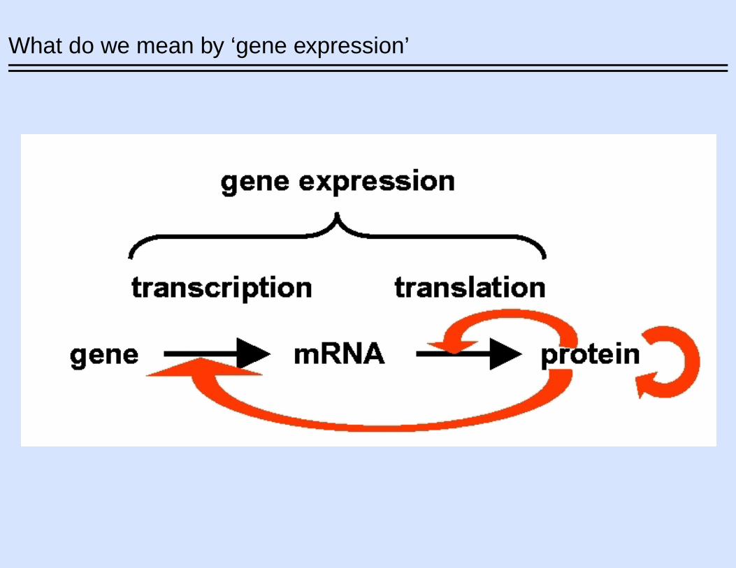
What do we mean by ‘gene expression’

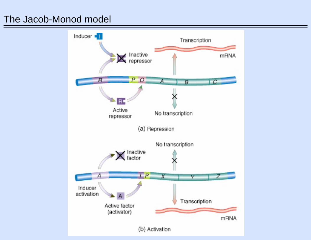
The Jacob-Monod model

The four basic modes of transcription control

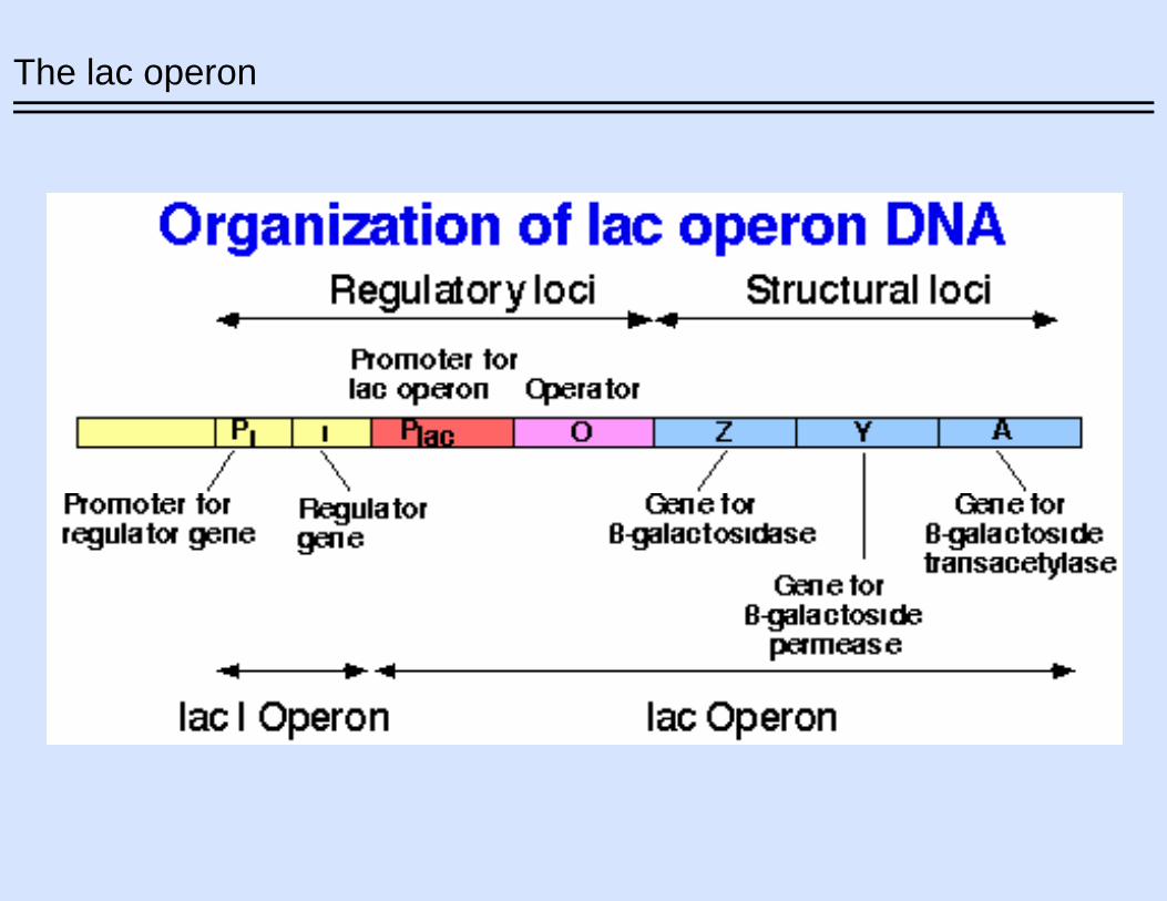
The lac operon

The effect of lactose

Eucaryotic transcription control

The loci of control and modification

Four types of models

• Boolean models

.... in which everything is either ON or OFF and the state space is a finite set

• Mixed models

.... in which some things are either ON or OFF, while others vary continuously

• Deterministic continuous models

.... in which everything varies continuously, the state space is a subset ofRn,

and the dynamics are deterministic

• Stochastic models

.... in which we recognize that ‘reactions ’ occur one molecule at a time

The Boolean approach

One realization of the ‘not if’ or ‘C and (not D)’

A general description of a gene control pathway based on feedback

The governing equations for a ‘continuous’ description

dS1

dt= R(Sn+1)− AN

VNT1(S1, S2)− k1S1

dS2

dt=ANVC

T1(S1, S2)− k2S2

dS3

dt= k2S2 − k3S3

dS4

dt= k3S3 − k4S4

...dSjdt

= kj−1Sj−1 − kjSj , j = 5, . . . , n− 1...dSndt

= kn−1Sn−1 − knSn −ANVC

Tn(Sn, Sn+1)

dSn+1

dt=ANVN

Tn(Sn, Sn+1)− kn+1Sn+1

wherekj = kj + kj for 4 ≤ j ≤ n− 1.

The control functions for inducible and repressible systems

R+ pS RSp, K1 = RSp/R · Sp

R+O OR, K2 = OR/R ·O

R = repressor,O = operator, andS = effector.

Rt = R+RSp = R(1 +K1Sp)

Ot = O +OR = O(1 +K2R)

Fraction of operator regions free of repressor:

f(S) =O

Ot=

1 +KtSp

K +K1Sp(2)

K = 1 +K2Rt > 1

For a repressible system

R+ pSK1� RSp

RSp +OK2� ORSp

In this case

f(S) =1 +K1S

p

1 +K1KSp(3)

Quantitative characterization of some gene control systems

Enzyme Effector p K1 K2Rt

Inducible

β-Galactosidase Isopropylthio- 1.91 2.5× 1010M−2 2.5× 103

galactoside

Histidine-NH3-lyase Imadizole 2.04 1.7× 1010M−2 26

propionate

Urocanase Histidine 2.3 4.3× 1012M−2 102

Mannitiol Ribitol 3.13 — —

dehydrogenase

Repressible

IMP dehydrogenase Guanine 0.91 —

XMP aminase Guanine 0.68 —

Alkaline PO3−4 0.93 2× 103M−1 5× 103

aFrom Yagil and Yagil (1971).