an introduction to lie algebra - scholarworks.lib.csusb.edu
TRANSCRIPT
California State University, San Bernardino California State University, San Bernardino
CSUSB ScholarWorks CSUSB ScholarWorks
Electronic Theses, Projects, and Dissertations Office of Graduate Studies
12-2017
An Introduction to Lie Algebra An Introduction to Lie Algebra
Amanda Renee Talley California State University – San Bernardino
Follow this and additional works at: https://scholarworks.lib.csusb.edu/etd
Part of the Algebra Commons
Recommended Citation Recommended Citation Talley, Amanda Renee, "An Introduction to Lie Algebra" (2017). Electronic Theses, Projects, and Dissertations. 591. https://scholarworks.lib.csusb.edu/etd/591
This Thesis is brought to you for free and open access by the Office of Graduate Studies at CSUSB ScholarWorks. It has been accepted for inclusion in Electronic Theses, Projects, and Dissertations by an authorized administrator of CSUSB ScholarWorks. For more information, please contact [email protected].
An Introduction to Lie Algebra
A Thesis
Presented to the
Faculty of
California State University,
San Bernardino
In Partial Fulfillment
of the Requirements for the Degree
Master of Arts
in
Mathematics
by
Amanda Renee Talley
December 2017

An Introduction to Lie Algebra
A Thesis
Presented to the
Faculty of
California State University,
San Bernardino
by
Amanda Renee Talley
December 2017
Approved by:
Dr. Giovanna Llosent, Committee Chair Date
Dr. Gary Griffing, Committee Member
Dr. Hajrudin Fejzic, Committee Member
Dr. Charles Stanton, Chair, Dr. Corey Dunn
Department of Mathematics Graduate Coordinator,
Department of Mathematics
iii
Abstract
An (associative) algebra is a vector space over a field equipped with an associa-
tive, bilinear multiplication. By use of a new bilinear operation, any associative algebra
morphs into a nonassociative abstract Lie algebra, where the new product in terms of the
given associative product, is the commutator. The crux of this paper is to investigate the
commutator as it pertains to the general linear group and its subalgebras. This forces
us to examine properties of ring theory under the lens of linear algebra, as we determine
subalgebras, ideals, and solvability as decomposed into an extension of abelian ideals, and
nilpotency, as decomposed into the lower central series and eventual zero subspace. The
map sending the Lie algebra L to a derivation of L is called the adjoint representation,
where a given Lie algebra is nilpotent if and only if the adjoint is nilpotent. Our goal is
to prove Engel’s Theorem, which states that if all elements of L are ad-nilpotent, then L
is nilpotent.
iv
Acknowledgements
I would like to thank the members of my Graduate Committee: Dr. Giovanna
Llosent, Dr. Gary Griffing, and Dr. Hajrudin Fejzic for their invaluable guidance and
patience in helping me construct and review this document. I would also like to thank
my husband, Andrew Wood, for his continued resilience and support throughout this
endeavor.

v
Table of Contents
Abstract iii
Acknowledgements iv
List of Figures vi
1 Introduction 1
2 Definitions and First Examples 112.1 The Notion of a Lie Algebra and Linear Lie Algebras . . . . . . . . . . . . 112.2 Classical Lie Algebras . . . . . . . . . . . . . . . . . . . . . . . . . . . . . 132.3 Lie Algebras of Derivations . . . . . . . . . . . . . . . . . . . . . . . . . . 172.4 Abstract Lie Algebras . . . . . . . . . . . . . . . . . . . . . . . . . . . . . 19
3 Ideals and Homomorphisms 233.1 Ideals . . . . . . . . . . . . . . . . . . . . . . . . . . . . . . . . . . . . . . 233.2 Homomorphisms and Representations . . . . . . . . . . . . . . . . . . . . 293.3 Automorphisms . . . . . . . . . . . . . . . . . . . . . . . . . . . . . . . . . 37
4 Solvable and Nilpotent Lie Algebras 424.1 Solvability . . . . . . . . . . . . . . . . . . . . . . . . . . . . . . . . . . . . 424.2 Nilpotency . . . . . . . . . . . . . . . . . . . . . . . . . . . . . . . . . . . . 454.3 Proof of Engel’s Theorem . . . . . . . . . . . . . . . . . . . . . . . . . . . 49
5 Conclusion 53
Bibliography 54
vi
List of Figures
3.1 Table of eigenvalues . . . . . . . . . . . . . . . . . . . . . . . . . . . . . . 273.2 Table of eigenvalues for B2 . . . . . . . . . . . . . . . . . . . . . . . . . . 343.3 Table of eigenvalues for C2 . . . . . . . . . . . . . . . . . . . . . . . . . . . 353.4 Table of eigenvalues for A3 and D3 . . . . . . . . . . . . . . . . . . . . . . 36

1
Chapter 1
Introduction
Abstract Lie algebras are algebraic structures used in the study of Lie groups.
They are vector space endomorphisms of linear transformations that have a new operation
that is neither commutative nor associative, but referred to as the bracket operation, or
commutator. Recall that an associative algebra preserves bilinear multiplication between
elements in a vector space V over a field F , where V ×V → V is defined by (x, y)→ xy for
x, y ∈ V . The bracket operation yields a new bilinear map, over the same vector space,
that turns any associative algebra into a Lie Algebra, where V × V → V is now defined
by [x, y] → (xy − yx). Central to the study of Lie algebras are the classical algebras,
which will be explored throughout this paper to derive isomorphisms, identify simple
algebras, and determine solvability. After examining some natural Lie algebra examples,
we will delve into the derived algebra, which is analogous to the commutator subgroup of
a group, and make use of it to define a sequence of ideals called the derived series, which
is solvable. We will then use a different sequence of ideals called the descending central
series to classify nilpotent algebras. All of this will arm us with the necessary tools to
prove Engel’s Theorem, which states that if all elements of L are ad-nilpotent, then L is
nilpotent. We must first recall some basic group axioms, ring axioms, and vector space
properties as a precursor to the study of Lie algebra.

2
The study of Lie Algebra requires a thorough understanding of linear algebra,
group, and ring theory. The following provides a cursory review of these subjects as
they will appear within the scope of this paper. Unless otherwise stated, our refresher
for group theory was derived from Aigli Papantonopoulou’s text Algebra Pure and
Applied [Aig02].
Definition 1.1. An associative algebra is an algebra A whose associative rule is associa-
tive: x(yz) = (xy)z for all x, y, z ∈ A
Definition 1.2. A nonempty set G equipped with an operation ∗ on it is said to form
a group under that operation if the operation obeys the following laws, called the group
axioms:
• Closure: For any a, b ∈ G, we have a ∗ b ∈ G.
• Associativity: For any a, b, c ∈ G, we have a ∗ (b ∗ c) = (a ∗ b) ∗ c.
• Identity: There exists an element e ∈ G such that for all a ∈ G we have a ∗ e =
e ∗ a = a. Such an element e ∈ G is called an identity in G.
• Inverse: For each a ∈ G there exists an element a−1 ∈ G such that a ∗ a−1 =
a−1 ∗ a = e. Such an element a−1 ∈ G is called an inverse of a in G.
Proposition 1.3. (Basic group properties) For any group G
• The identity element of G is unique.
• For each a ∈ G, the inverse a−1 is unique.
• For any a ∈ G, (a−1)−1 = a
• For any a, b ∈ G, (ab)−1 = b−1a−1
• For any a, b ∈ G, the equations ax = b and ya = b have unique solutions or, in
other words, the left and right cancellation laws hold.
Example 1.0.1. The general linear group, denoted gl(n), consists of the set of invert-
ible n × n matrices. By the above, given that multiplication of invertible n × n matrices
is associative, and each invertible matrix has an inverse and an identity, gl(n) forms a
group under multiplication.
3
Definition 1.4. nonempty subset H of a group G is a subgroup of G if H is a group
under the same operation as G. We use the notation H ⊂ G to mean that H is a subset
of G, and H ≤ G to mean that H is a subgroup of G. For a group G with identity element
e, {e} is a subgroup of G called the trivial subgroup. For any group G, G itself is a
subgroup of G, called the improper subgroup. Any other subgroup of G besides the two
above is called a nontrivial proper subgroup of G.
Definition 1.5. The number of elements in a group G is called the order of G and is
denoted |G|. G is a finite group if |G| is finite. If a ∈ G, the order |a| of a in G is
the least positive integer n such that an = e. If there exists no such integer n, then |a| is
infinite.
Definition 1.6. A map ϕ : G → G′
from a group G to a group G′ is called a homo-
morphism if ϕ(ab) = ϕ(a)ϕ(b) for all a, b ∈ G (in ϕ(ab) the product is being taken in
G, while in ϕ(a)ϕ(b) the product is being taken in G′).
Proposition 1.7. (Basic group homomorphism properties) Let ϕ : G → G′ be a
homomorphism. Then
• ϕ(e) = e′, where e is the identity of G and e′ the identity of G′.
• ϕ(a−1) = (ϕ(a))−1 for any a ∈ G
• ϕ(an) = ϕ(a)n for any n ∈ Z
• If |a| is finite, then |ϕ(a)| divides |a|.
• If H is a subgroup of G, then ϕ(H) = {ϕ(x)|x ∈ H} is a subgroup of G′
• If K is a subgroup of G′, then ϕ−1(K) = {x ∈ G|ϕ(x) ∈ K} is a subgroup of G.
Example 1.0.2. For any group G, the identity map is always a homomorphism, since
if ϕ : G→ G′ is the identity ϕ(x) = x, then ϕ(xy) = xy = ϕ(x)ϕ(y)
Definition 1.8. For the homomorhpism ϕ, the kernel of ϕ is the set {x ∈ G|ϕ(x) = e′},denoted Ker ϕ.
Definition 1.9. Let G be a group, H a subgroup of G, and a ∈ G. Then the set aH =
{aH|h ∈ H} is called a left coset of H in G, and the set Ha = {ha|h ∈ H} is called a
right coset of H in G.
4
Definition 1.10. The group consisting of the cosets of H in G under the operation
(aH)(bH) = (ab)H is called the quotient group of G by H, written G/H.
Definition 1.11. If G is any group, then the center of G, denoted Z(G), consists of the
elements of G that commute with every element of G. In other words,
Z(G) = {x ∈ G|xy = yx ∀y ∈ G} (1.1)
Note that ey = y = ye for all y ∈ G, so e ∈ Z(G), and the center is a nonempty subset of
G. Let a ∈ G. Then the centralizer of a in G, denoted CG(a), is the set of all elements
of G that commute with a. In other words
CG(a) = {y ∈ G|ay = ya} (1.2)
Note that for any a ∈ G we have Z(G) ⊆ CG(a). In other words, the center is contained
in the centralizer of any element [Aig02].
Definition 1.12. Let G be a group and H a subgroup of G. If for all g ∈ G we have
gH = Hg, then we say H is a normal subgroup of G and write H/G. (Recall the normal
subgroup test: A subgroup H of G is normal in G if and only if xHx−1 ⊆ H for all x in
G) .
The following material for group and ring theory was derived from Joseph A.
Gallian’s Contemporary Abstract Algebra [Gal04].
Definition 1.13. An isomorphism from a group G onto itself is called an automor-
phism of G.
Definition 1.14. Let G be a group, and let a ∈ G. The function ϕa defined by ϕa(x) =
axa−1 for all x ∈ G is called the inner automorphism of G induced by a.
Definition 1.15. A set R equipped with two operations, written as addition and multi-
plication, is said to be a ring if the following four ring axioms are satisfied, for any
elements, a, b, and c in R:
• R is an Abelian group under addition.
• Closure: ab ∈ R
5
• Associativity: a(bc) = (ab)c.
• Distributivity: a(b+ c) = ab+ ac and (b+ c)a = ba+ ca.
Definition 1.16. A subring A of a ring R is called a (two-sided) ideal of R if for every
r ∈ R and every a ∈ A both ra and ar are in A.
Theorem 1.17. Ideals are Kernels Every ideal of a ring R is the kernel of a ring
homomorphism of R. In particular, an ideal A is the kernel of the mapping r → r + A
from R to R/A.
Definition 1.18. A unity (or identity) in a ring is a nonzero element that is an identity
under multiplication. A nonzero element of a commutative ring with unity that has a
multiplicative inverse is called a unit of the ring.
Theorem 1.19. First Isomorphism Theorem for Rings Let ϕ be a ring homomor-
phism from R→ S. Then the mapping from R/kerϕ to ϕ(r), given by r + kerϕ→ ϕ(r)
is an isomorphism. In symbols, R/kerϕ ∼= ϕ(r)
Theorem 1.20. Second Isomorphism Theorem for Rings If A is a subring of R
and B an ideal of R, then A∩B is an ideal of A and A/A∩B is isomorphic to (A+B)/B.
(Recall that {A+B = a+ b|a ∈ A, b ∈ B})
Theorem 1.21. Third Isomorphism Theorem for Rings Let A and B be ideals of
a ring R with B ⊆ A. A/B is an ideal of R/B and (R/B)(A/B) is isomorphic to R/A.
Theorem 1.22. Correspondence Theorem Let I be an ideal of a ring R. There exists
a bijection between the set of all ideals J of R such that I ⊂ J and the set of all ideals of
R/I:
{J |I is an ideal of R, I ⊂ J} → {K|K is an ideal of r/I}
J → J/I
Definition 1.23. In a ring R the characteristic of R, denoted char R, is the least
positive integer n such that n · a = 0 for all a ∈ R. If no such n exists, we say char
R = 0.
Definition 1.24. A field is a commutative ring with unity in which every nonzero ele-
ment is a unit.
6
Unless otherwise stated, the material for our vector space review was derived
from Stephen H. Friedberg et al’s, Linear Alebra [FIS03].
Definition 1.25. Let F be a field. A set V equipped with two operations, written as
addition and multiplication, is said to be a vector space over F if
• V is an Abelian group under addition. For all a, b ∈ F and all u, v ∈ V ,
• The product av ∈ V is defined
• a(v + w) = av + aw
• a(bv) = (ab)v
• 1v = v
An element of v ∈ V is called a vector. The identity element of V under addition is
called the zero vector and written 0. An element of a ∈ F is called a scalar, and the
operation of forming av is called scalar multiplication [Aig02].
Definition 1.26. A subset U of a vector space V over a field F is called a subspace of
V if U is a vector space over F with the operations of addition and scalar multiplication
defined on V
Example 1.0.3. If T : V →W is a linear map, the kernel of T and the image (range)
of T defined by
ker(T ) = {x ∈W : T (x) = 0}
im(T ) = {w ∈W : T (x), x ∈W}
are subspaces of V .
Definition 1.27. Let V be a vector space over a field F. A vector space homomorphism
that maps V to itself is called an endomorphism of V
Definition 1.28. Let V and W be vector spaces. We say that V is isomorphic to W if
there exists a linear transformation T : V →W that is invertible. Such a transformation
is called an isomorphism from V to W .
7
Definition 1.29. Let V be a vector space over C. An inner product on V is a function
that assigns, to every ordered pair of vectors x and y in V , a scalar in C, denoted 〈x, y〉,such that for all x, y, z in V and all c in C, the following hold:
1. 〈x+ z, y〉 = 〈x, y〉+ 〈z, y〉
2. 〈cx, y〉 = c 〈x, y〉
3. 〈x, y〉 = 〈y, x〉
4. 〈x, x〉 > 0 if x 6= 0
Definition 1.30. Let V be a vector space over a field F . A function f from the set V ×Vof ordered pairs of vectors to F is called a bilinear form on V if f is linear in each
variable when the other variable is held fixed; that is, f is a bilinear form on V if
1. f(αx1 + x2, y) = αf(x1, y) + f(x2, y)
2. f(x, αy1 + y2) = αf(x, y1) + f(x, y2)
Any nondegenerate bilinear form on V consists of all operators x on V un-
der which the form f is infinitesimally invariant, i.e., that satisfies f(x(v), w) +
f(v, x(w)) = 0. [FIS03]
The kernel of a symmetric bilinear form is given as: kerf = {v : f(v, w) = 0 for all w ∈ V }.That is, for all v ∈W , there exists a w ∈ V such that f(v, w) = 0.
Definition 1.31. An alternating space is defined as the set of all vector spaces V and
alternate bilinear forms such that f : V × V → F where:
1. f(x, y + z) = f(x, y) + f(x, z)
2. f(x+ y, z) = f(x, z) + f(y, z)
3. f(ax, y) = af(x, y) = f(x, ay)
4. f(x, x) = 0 which implies that f(x, y)=-f(y,x)
Definition 1.32. In matrix terms, an n-linear function γ : Mn×n(F ) → F is called
alternating if, for each A ∈ Mn×n(F ), we have γ(A) = 0 whenever two adjacent rows
of A are equal. [FIS03]
8
Theorem 1.33. Let A be an m× n matrix, B and C be n× p matrices and D and E be
q ×m matrices. Then
1. A(B + C) = AB +AC and (D + E)A = DA+ EA
2. α(AB) = (αA)B = (AαB)
3. ImA = A = AIm
4. If V is an n-dimensional vector space with an ordered basis B, then [IV ]B = In
Definition 1.34. Let A,B and C be matrices where C = cij, A = ajk, and B = bkj.
Then by matrix multiplication
C = AB where cij =n∑k=1
aikbkj
The formula for the determinant of A, denoted det(A) or |A|, where A is a n× nmatrix can be expressed as cofactor expansion along the 1st row of A
det(A) =
n∑j=1
(−1)i+jAij · det(Aij)
Where the scalar cij = (−1)i+jdet(Aij) is called the cofactor of the entry of A if row i,
column j.
Example 1.0.4. The Laplace expansion of A where A is a 2× 2 matrix is
det(A) = A11(−1)1+1detA11 +A12(−1)1+2detA12
Definition 1.35. (Adjoint of a Matrix) Let A be an n× n matrix. The matrix B = [bij ]
with bij = cji (for cij as defined in Definition 1.33), for 1 ≤ i, j ≤ n is called the Adjoint
of A, denoted Adj(A).
Definition 1.36. The trace of a matrix is the sum of its diagonal entries.
Definition 1.37. Given an n × n matrix A = {aij}, the transpose of A is the matrix
AT = {bij}, where bij = aji.
Definition 1.38. If the transpose of a matrix is equal to the negative of itself, the matrix
is said to be skew symmetric. This means that for a matrix to be skew symmetric,
At = −A.
9
Definition 1.39. Let F be a field and V,W vector spaces over the field F . A function
T : V →W is said to be a linear transformation from V to W if for all c, d ∈ F , and
all x, y ∈ V we have
T (cx+ yd) = cT (x) + dT (y)
The following are simple properties of linear transformations:
• T (0) = 0
• T (cx+ y) = cT (x) + T (y)
• T (x− y) = T (x)− T (y)
• For x1, x2, ..., xn ∈ V and a1, a2, ..., an ∈ F , we have
T (n∑i=1
aixi) =n∑i=1
aiT (xi)
Example 1.0.5. Consider the map T : Mn×n(F ) → Mn×m(F ) defined by T (A) = At.
We can show that T is a linear transformation. Let A = Aij and B = Bij
(A+B)t = (Aij +Bij)t = (Aij)
t + (Bij)t = At +Bt
T (cAij) = (cAij)t = c(Aij)
t = cAt
Definition 1.40. A basis, β, for a vector space V is a linearly independent subset of V
that generates V . If there exists a finite set that forms a basis for V over a field F , then
the number n of vectors in such a basis {v1...vn} is called the dimension of V over F ,
written dim FV . If there exists no finite basis for V over F , then V is said to be infinite
dimensional over F .
Definition 1.41. Let T = TA : V → V be a linear transformation, where V is a finite-
dimensional vector space over a field F , and let 0 6= v ∈ V be such that TA(v) = λv for
some λ ∈ F . Then v is called an eigenvector of T (and of A), and λ the corresponding
eigenvalue of T (and of A).
Definition 1.42. A is invertible if there exists an n × n matrix B such that AB =
BA = I.
10
Definition 1.43. a matrix M ∈Mn×n(F ) is called orthogonal if MM t = I.
Theorem 1.44. If A is a square matrix of order n > 1, then A(adjA) = (adjA)A =
|A|In. The (i, j)th element of A(adjA) is:
n∑k=1
aikakj =n∑k=1
aijAjk =
|A| ⇔ i = j
0⇔ i 6= j
Therefore A(adjA) is a scalar matrix with diagonal elements all equal to |A|.
⇒ A(AdjA) = I(n)
⇒ (AdjA)A = |A|I(n)
Where |A| represents the determinant of A.[Eve66]
Proposition 1.45. The following equation denotes the inverse of A:
A−1 =AdjA
|A|
Definition 1.46. If A is a square matrix of order n, then the λ matrix [A − λI(n)]
is called the characteristic matrix of A. The determinant |A − λI(n)| is called the
characteristic determinant of A, and the expansion of it is a polynomial of degree n:
f(λ) = (−1)n[λn − p1λn−1 + p2λn−2 + ...( − 1)npn]
[Eve66]
Theorem 1.47. In the characteristic function f(λ) of matrix A, pn = |A| and p1 = trA.
[Eve66]
11
Chapter 2
Definitions and First Examples
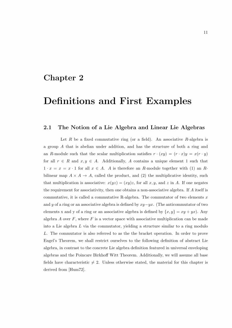
2.1 The Notion of a Lie Algebra and Linear Lie Algebras
Let R be a fixed commutative ring (or a field). An associative R-algebra is
a group A that is abelian under addition, and has the structure of both a ring and
an R-module such that the scalar multiplication satisfies r · (xy) = (r · x)y = x(r · y)
for all r ∈ R and x, y ∈ A. Additionally, A contains a unique element 1 such that
1 · x = x = x · 1 for all x ∈ A. A is therefore an R-module together with (1) an R-
bilinear map A × A → A, called the product, and (2) the multiplicative identity, such
that multiplication is associative: x(yz) = (xy)z, for all x, y, and z in A. If one negates
the requirement for associativity, then one obtains a non-associative algebra. If A itself is
commutative, it is called a commutative R-algebra. The commutator of two elements x
and y of a ring or an associative algebra is defined by xy−yx. (The anticommutator of two
elements x and y of a ring or an associative algebra is defined by {x, y} = xy + yx). Any
algebra A over F , where F is a vector space with associative multiplication can be made
into a Lie algebra L via the commutator, yielding a structure similar to a ring modulo
L. The commutator is also referred to as the the bracket operation. In order to prove
Engel’s Theorem, we shall restrict ourselves to the following definition of abstract Lie
algebra, in contrast to the concrete Lie algebra definition featured in universal enveloping
algebras and the Poincare Birkhoff Witt Theorem. Additionally, we will assume all base
fields have characteristic 6= 2. Unless otherwise stated, the material for this chapter is
derived from [Hum72].

12
Definition 2.1. A vector space L over a field F , is a Lie algebra if there exists a bilinear
multiplication L× L→ L, with an operation, denoted (x, y) 7→ [xy], such that:
1. It is skew symmetric where [x, x] = 0 for all x in L (this is equivalent to
[x, y] = −[y, x] since character F 6= 2).
2. It satisfies the Jacobi identity [x[yz]] + [y[zx]] + [z[xy]] = 0 (x, y, z ∈ L).
Example 2.1.1. Given an n dimensional vector space End (V ), the set of all all linear
maps V 7→ V with associative multiplication (x, y) 7→ xy for all x, y, where xy denotes
functional composition, observe, End (V ) is an associative algebra over F . Let us define
a new operation on End (V ) by (x, y) 7→ xy − yx. If we denote xy − yx by [x, y], then
End (V ) together with the map [·, ·] satisfies Definition 2.1, and is thus a Lie algebra.
Proof. The first two bracket axioms are satisfied immediately. The only thing left to
prove is the Jacobi identity. Given x, y, z ∈ End (V ), we have by use of the bracket
operation:
[x[yz]] + [y[zx]] + [z[xy]] = 0
= x(yz − zy)− (yz − zy)x+ y(zx− xz)− (zx− xz)y + z(xy − yx)− (xy − yx)z
= xyz − xzy − yzx+ zyx+ yzx− yxz − zxy + xzy + zxy − zyx− xyz + yxz
= (xyz − xyz) + (xzy − xzy) + (yzx− yzx) + (zyx− zyx) + (yxz − yxz) = 0
Definition 2.2. The Lie algebra End (V ) with bracket [x, y] = xy − yx, is denoted as
gl(V ), the general linear algebra.
Example 2.1.2. We can show that real vector space R3 is a Lie algebra. Recall the
following cross product properties when a, b and c represent arbitrary vectors and α, β
and γ represent arbitrary scalars:
1. a× b = −(b× a),
2. α× (βb+ γc) = β(a× b) + γ(a× c) and
(αa+ βb)× c = α(a× c) + β(b× c),

13
([MT03])
Note, a× a = −(a× a), by property (1), letting b = a, therefore, a× a = 0. By the above
properties, the cross product is both skew symmetric (property 1) and bilinear (property
2). By vector triple product expansion: x× (y× z) = y(x · z)− z(x · y). To show that the
cross product satisfies the Jacobi identity, we have:
[x[y, z]] + [y[z, x]] + [z[x, y]] = x× (y × z) + y × (z × x) + z × (x× y)
= [y(x · z)− z(x · y)] + [z(y · x)− x(y · z)] + [x(z · y)− y(z · x)]
= 0 {Since the dot product is commutative}
Therefore, by definition 2.1, the real vector space R3 is a Lie algebra
Definition 2.3. A subspace K of L is called a (Lie) subalgebra if [xy] ∈ K whenever
x, y ∈ K.
2.2 Classical Lie Algebras
Classical algebras are finite-dimensional Lie algebras. Each classical algebra Al,
Bl, Cl, and Dl has an associated algebra, represented by symmetric, skew symmetric, and
orthogonal matrices. Let s be an n×n matrix. We shall prove that each classical algebra
representation, equipped with basis and dimension satisfying xs+sxt = 0 (xt =transpose
of x), is a subalgebra of the linear Lie algebra gl(V ). Note: a proper subalgebra maintains
dimension less than that of gl(n).
(Al) The set of all endomorphisms of V having trace zero is denoted by sl(V ), the
special linear algebra. Letting x, y ∈ sl(V ), we can show that sl(V ) is a subalgebra of
gl(V ).
Proof.
tr[x, y] = tr(xy)− tr(yx) = 0 {Since the trace of a matrix preserves bilinearity}
tr([x, [y, z]] + [y, [z, x]] + [z, [x, y]]) = tr[x, 0] + tr[y, 0] + tr[z, 0] = 0
Therefore, both Lie algebra axioms are satisfied, hence by Definition 2.3, sl(V ) is a
subalgebra of gl(V ).

14
The dimension of sl(V ) is found by determining the number of linearly independent
matrices of sl(V ) that yield trace 0. By counting the matrices eij(i 6= j), and adding
them to the matrices hi = eij − ei+1,i+1, we find dim sl(V ) = l + (l + 1)2 − (l + 1)
(Cl) The set of endomorphisms of V having dim V = 2l, that satisfies
f(v, w) = −f(w, v), is denoted as sp(V ), the symplectic algebra. Let s be a
nondegenerate, skew symmetric matrix where s =
0 Il
−Il 0
. Recall that a matrix
A ∈Mn×n(F ) is called skew-symmetric if At = −A. We can show sp(2l, F ) is a
subalgebra of gl(V ) if we partition x as x =
m n
p q
where m,n, p, q ∈ gl(v).
Proof. Given x, y ∈ sp(V ),
f([xy](v), w) + f(v, [xy](w))
=f((xy − yx)v, w) + f(v, (xy − yx)w) {By definition of the bracket operation}
=f(xy(v), w)− f(yx(v), w) + f(v, xy(w))− f(v, yx(w)) {By definition of bilinearity}
=f(x(y(v)), w)− f(y(x(v)), w) + f(v, x(y(w))− f(v, (y(x(w))
=− f(y(v), x(w)) + f(x(v), y(w))− f(x(v), y(w)) + f(y(v), x(w)) {By skew symmetry}
=0
Therefore [x, y] ∈ sp(V ), hence sp(V ) is a subalgebra of gl(V ) when sp(v) is of even
dimension. We show that sp(V ) requires even dimensionality by considering the
determinant of x when n is odd. From sx = −xts,
det(sx) = det(−xts) ⇐⇒ det(s)det(x) = det(−xt)det(s)
⇐⇒ det(x) = det(−xt)
= (−1)ndet(xt)
= (−1)2k−1det(xt)
= −det(xt)
but then det(x) = −det(xt), therefore, det(x) = 0
(Bl) The set of all endomorphisms of V with dimension 2l2 + l satisfying
f(x(v), w) = −f(v, x(w)), such that f is a non-degenerate bilinear form on V with
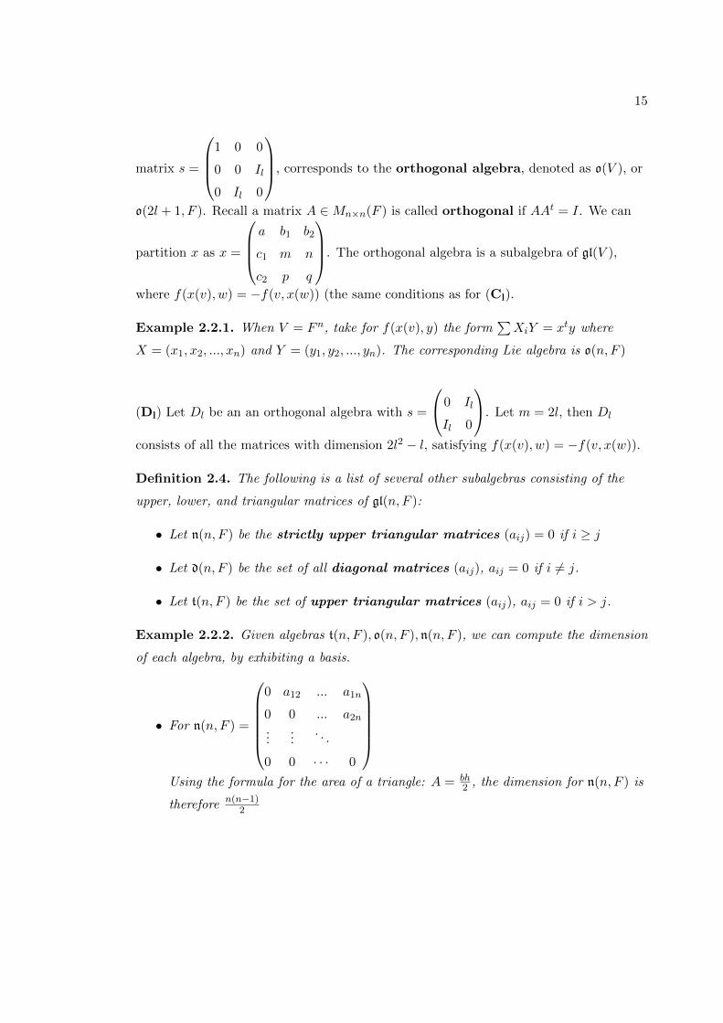
15
matrix s =
1 0 0
0 0 Il
0 Il 0
, corresponds to the orthogonal algebra, denoted as o(V ), or
o(2l + 1, F ). Recall a matrix A ∈Mn×n(F ) is called orthogonal if AAt = I. We can
partition x as x =
a b1 b2
c1 m n
c2 p q
. The orthogonal algebra is a subalgebra of gl(V ),
where f(x(v), w) = −f(v, x(w)) (the same conditions as for (Cl).
Example 2.2.1. When V = Fn, take for f(x(v), y) the form∑XiY = xty where
X = (x1, x2, ..., xn) and Y = (y1, y2, ..., yn). The corresponding Lie algebra is o(n, F )
(Dl) Let Dl be an an orthogonal algebra with s =
0 Il
Il 0
. Let m = 2l, then Dl
consists of all the matrices with dimension 2l2 − l, satisfying f(x(v), w) = −f(v, x(w)).
Definition 2.4. The following is a list of several other subalgebras consisting of the
upper, lower, and triangular matrices of gl(n, F ):
• Let n(n, F ) be the strictly upper triangular matrices (aij) = 0 if i ≥ j
• Let d(n, F ) be the set of all diagonal matrices (aij), aij = 0 if i 6= j.
• Let t(n, F ) be the set of upper triangular matrices (aij), aij = 0 if i > j.
Example 2.2.2. Given algebras t(n, F ), o(n, F ), n(n, F ), we can compute the dimension
of each algebra, by exhibiting a basis.
• For n(n, F ) =
0 a12 ... a1n
0 0 ... a2n...
.... . .
0 0 · · · 0
Using the formula for the area of a triangle: A = bh
2 , the dimension for n(n, F ) is
therefore n(n−1)2
16
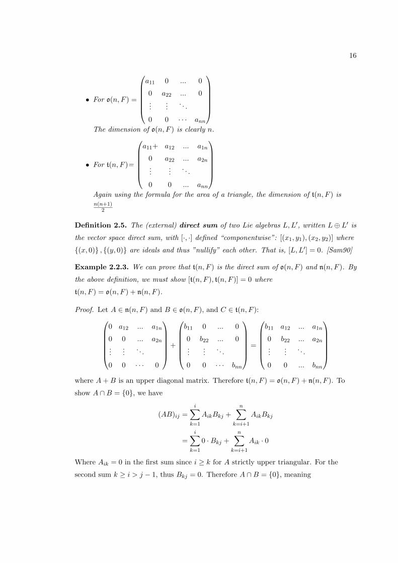
• For o(n, F ) =
a11 0 ... 0
0 a22 ... 0...
.... . .
0 0 · · · ann
The dimension of o(n, F ) is clearly n.
• For t(n, F )=
a11+ a12 ... a1n
0 a22 ... a2n...
.... . .
0 0 ... ann
Again using the formula for the area of a triangle, the dimension of t(n, F ) isn(n+1)
2
Definition 2.5. The (external) direct sum of two Lie algebras L,L′, written L⊕ L′ is
the vector space direct sum, with [·, ·] defined “componentwise”: [(x1, y1), (x2, y2)] where
{(x, 0)} , {(y, 0)} are ideals and thus ”nullify” each other. That is, [L,L′] = 0. [Sam90]
Example 2.2.3. We can prove that t(n, F ) is the direct sum of o(n, F ) and n(n, F ). By
the above definition, we must show [t(n, F ), t(n, F )] = 0 where
t(n, F ) = o(n, F ) + n(n, F ).
Proof. Let A ∈ n(n, F ) and B ∈ o(n, F ), and C ∈ t(n, F ):0 a12 ... a1n
0 0 ... a2n...
.... . .
0 0 · · · 0
+
b11 0 ... 0
0 b22 ... 0...
.... . .
0 0 · · · bnn
=
b11 a12 ... a1n
0 b22 ... a2n...
.... . .
0 0 ... bnn
where A+B is an upper diagonal matrix. Therefore t(n, F ) = o(n, F ) + n(n, F ). To
show A ∩B = {0}, we have
(AB)ij =i∑
k=1
AikBkj +n∑
k=i+1
AikBkj
=
i∑k=1
0 ·Bkj +n∑
k=i+1
Aik · 0
Where Aik = 0 in the first sum since i ≥ k for A strictly upper triangular. For the
second sum k ≥ i > j − 1, thus Bkj = 0. Therefore A ∩B = {0}, meaning
17
AB −BA = [AB] = 0. Therefore [o(n, F ), n(n, F )] ⊆ n(n, F ). We can construct a basis
eij for n(n, F ) such that eij is 1 for the (ij) element, and zero elsewhere. By definition
of the commutator:
[eii, eij ] = eiieij − eijeii = eij
By the above, when i ≥ j, n(n, F ) ⊆ [o(n, F ), n(n, F )], and thus
[o(n, F ), n(n, F )] = n(n, F ). Since o(n, F ) + n(n, F ) = t(n, F ):
[o(n, F ) + n(n, F ), o(n, F ) + n(n, F )] = [o(n, F ), o(n, F )] + [n(n, F ), n(n, F )]
[n(n, F ), o(n, F )] + [o(n, F ), n(n, F )]
= 0 + 0 + [o(n, F ), n(n, F )] ⊆ n(n, F )
Conversely:
n(n, F ) = [o(n, F ), n(n, F )] ⊆ [t(n, F ), t(n, F )]
Therefore [t(n, F ), t(n, F )] = n(n, F ) and thus t(n, F ) = o(n, F ) + n(n, F )
2.3 Lie Algebras of Derivations
The derivative between two functions f and g is a linear operator that satisfies the
Leibniz rule:
1. (fg)′ = f ′g + fg′
2. (αf)′ = αf ′ where α is a scalar.
Given an algebra A over a field F , the derivation of A is the linear map δ such that
δ(f, g) = fδ(g) + δ(f)g for all f, g ∈ A. The set of all derivations of A is denoted by
Der(A). Given δ ∈ Der(A), f, g ∈ A, and α ∈ F . By property 2.,
(αδ)(fg) = αδ(fg) = α(fδ(g) + δ(f)g) = αfδ(g) + αδ(f)g
where the Leibniz rule is satisfied if and only if af = fa where F is a field.
Example 2.3.1. Let x, y ∈ End(V ), and δ, δ′ ∈ Der(V ). By definition of the
commutator, [δ, δ′] = (δδ′ − δ′δ):
18
• Der(V ) is a vector subspace of End(V ):
δ[x, y] = δ(xy − yx) = δ(xy)− δ(yx)
= xδ(y) + δ(x)y − (yδ(x) + δ(y)x)
= δ(y)x− yδ(x) + xδ(y)− δ(y)x
= [δ(x), y] + [x, δ(y)]
• The commutator [δ, δ′] of two derivations δ, δ′ ∈ Der(V ) is again a derivation.
([δ, δ′](x))y + x([δ, δ′](y)) = ((δδ′ − δ′δ)(x))y + x(δδ′ − δ′δ)(y)
= (δδ′(x)− δ′δ(x))y + x(δδ′(y)− δ′δ(y))
= δδ′(x)y − δ′δ(x)y + xδδ′(y)− xδ′δ(y)
= δ(δ′(x)y + xδ′(y))− δ′(δ(x)y + xδ(y))
= δ(δ′(x)y) + δ′(x)δ(y) + δ(x)δ′(y) + xδ(δ′(y))
− δ′(δ(x)y)− δ(x)δ′(y)− δ′(x)δ(y)− xδ′δ(y)
= δ(δ′(x)y + xδ′(y))− δ′(δ(x)y + xδ(y))
= δ(δ′(xy))− δ′(δ(xy))
= [δ, δ′](xy)
Definition 2.6. Given x ∈ L, the map y → [x, y], is an endomorphism of L, denoted
adx, where adx is an inner derivation. Derivations of the form [x[yz]] = [[xy]z] + [y[xz]]
are inner. All others are outer.
Example 2.3.2. By example 2.3.1, the collection of derivations, Der(V ), satisfies skew
symmetry. By definition 2.6, Der(V ) satisfies the Jacobi identity. Therefore Der(V )
defines a Lie algebra.
Definition 2.7. The map L→ DerL sending x to adx is called the adjoint
representation of L.
This is akin to taking the ad homomorphism of g→ gl(g). To show ad is a
homomorphism:
ad([x,y]) = [ad(x), ad(y)] = ad(x)ad(y) − ad(y)ad(x)
19
if and only if:
[[x, y], z] = [x, [y, z]]− [y, [x, z]]
0 = [x, [y, z]] + [y, [z, x]] + [z, [x, y]]
That is, if and only if the Jacobi identity is satisfied, where [[x, y], z] = −[z, [x, y]] and
−[y, [x, z]] = [y, [z, x]] by skew symmetry.
Definition 2.8. A representation is faithful if its kernal is zero, i.e., if
φ(x) = 0⇔ x = 0, where the adjoint operator defines the trivial representation. [Sam90]
2.4 Abstract Lie Algebras
Let L be a finite dimensional vector space over F . Any vector space can be made into a
Lie algebra simply by setting [x, y] = 0 for all vectors x and y in L. The resulting Lie
algebra is called abelian. Recall that a group G under multiplication is said to be
Abelian if G obeys the commutative law or, that is, if for every a, b ∈ G we have
ab = ba [Aig02]. If an associative algebra is abelian and therefore commutative, then
ab = ba⇔ [a, b] = 0, where [a, b] is the associated commutator.
Example 2.4.1. Given L as a Lie algebra, with [xy] = 0 for all x, y ∈ L,
[xy] = (xy − yx) = 0⇔ xy = yx
Therefore L under trivial Lie multiplication, is abelian. Similarly, [yx] = 0.
Definition 2.9. If L is any Lie algebra with basis x1, ..., xn, then the multiplication
table for L is determined by the structural constants, the set of scalars {bijk} such
that [xi, xj ] =∑n
k=1 bijkxk.
Example 2.4.2. By use of the bracket axioms, the following set of structural constants
define an abstract Lie algebra:
1. biik = 0 = bijk + bjik
2.∑
(bijkbklm + bjlkbklm + blikbkjm) = 0
Proof.
20
1. Recall [xx] = 0 for all x ∈ L.
[xi, xi] = 0 =n∑k=1
biikxk
= bii1x1 + bii2x2 + ...+ biinxn = 0.
Then, since xi is a basis, biik = 0 for all k.
2. Given [xi, xj ] =∑n
k=1 bijkxk, notice bijk + bjik = 0 if and only if∑k
(bijk + bjik)xk = 0 :
⇔∑k
bijkxk +∑k
bjikxk = 0⇔ [xixj ] + [xjxi] = 0
But:
[xixj ] = xixj − xjxi
[xjxi] = xjxi − xixj
⇔ [xixj ] + [xjxi] = xixj − xjxi + xjxi − xixj = 0
Definition 2.10. The assorted systems of structural constants of a given Lie algebra
relative to its basis form an orbit (the set of all transformations of one element) under
this action [Sam90].
Example 2.4.3. The orbit of the system cijk = 0 for all i, j, k forms a natural
isomorphism to the abelian algebra [X,Y ] = 0 of dimension n.
Example 2.4.4. Consider a Lie algebra L with basis x1, ...xn. The structural constants
are enumerated as followed: e1 = (1, 0, 0), e2 = (0, 1, 0), and e3 = (0, 0, 1). By use of the
Lie bracket axioms, We have:
[e1, e2] = e3
[e1, e3] = −e2
[e2, e3] = e1

21
Therefore, by definition, the structural constants are:
b121 = 0, b122 = 0, b123 = 1,
b131 = 0, b132 = −1, b133 = 0,
b231 = 1, b232 = 0, b233 = 0
Example 2.4.5. We can use structural constants to show that a three dimensional
vector space with basis (x, y, z) such that [xy] = z, [xz] = y, [yz] = 0 defines a Lie
algebra.
Proof. the structural constants are:
b121 = b122 = 0, b123 = 1,
b131 = b133 = 0, b132 = 1,
b231 = b232 = b233 = 0
Where bijk = bijk − bjik = 0 for all structural constants above (by skew-symmetry). By
the Jacobi identity, we have:
[x[yz]] + [z[xy]] + [y[zx]] = [x, 0] + [z, z] + [y.− y] = 0 + 0 + 0 = 0
Therefore the above basis defines a Lie algebra structure over F .
Definition 2.11. For any field F , in the vector space
Fn = {(b1, b2, b3..., bn)|bi ∈ F for 1 ≤ i ≤ n}
a basis is formed by the vectors
e1 = (1, 0, ..., 0)
e2 = (0, 1, ..., 0)
...
en = (0, 0, ..., 1)
Where {e1, e2, ..., en} is called the standard basis for Fn over F .
Theorem 2.12. Let V and W be finite-dimensional vector spaces (over the same field).
Then V is isomorphic to W if and only if they are of equal dimension.

22
Corollary 2.13. Let V be a vector space over F . Then V is isomorphic to Fn if and
only if dim(V ) = n [FIS03]
Example 2.4.6. By Corollary 2.13, there exists an isomorphism between gl(n) and Fn.

23
Chapter 3
Ideals and Homomorphisms
3.1 Ideals
Lie algebra ideals are intrinsic to much that follow. In group theory, ideals are used to
define the kernel of a group, normal subgroups, and the structure of nilpotent and
solvable groups. In a ring, every kernal is an ideal of a homomorphism, and every
subgroup is normal. By definition of the normal subgroup, if H is a subgroup of G, for
all g ∈ G we have gH = Hg ⇔ [g,H] = 0. Unless otherwise stated, the material for this
chapter is derived from [Hum72].
Definition 3.1. A subspace I of a Lie algebra L is called an ideal of L if x ∈ I, y ∈ Ltogether imply [x, y] ∈ I. The construction of ideals in Lie algebra is analogous to the
construction of normal subgroups in group theory.
By skew-symmetry, all Lie algebra ideals are automatically two sided. That is, if
[x, y] ∈ I, then [y, x] ∈ I. The kernel of a Lie algebra L and L itself are trivial ideals
contained in every Lie algebra.
Example 3.1.1. The set of all inner derivations adx, x ∈ L, is an ideal of Der(L). Let
δ ∈ Der(L). By definition of inner derivations, for all y ∈ L:
[δ, adx](y) = (δ(adx)− (adx)δ)(y) = δ[x, y]− adx(δ(y))
= [δ(x), y] + [x, δ(y)]− [x, δ(y)] {Since δ[x, y] = [δ(x), y] + [x, δ(y)]}
= ad(δ(x)y)
Therefore, by Definition 3.1, adx is an ideal of Der(L).
24
Definition 3.2. The center of a Lie algebra L is the set
Z(L) = {z ∈ L|[x, z] = 0 for all x ∈ L}
The center respresents the collection of elements in L for which the adjoint action ad(z)
yeilds the zero derivation. It can therefore be thought of as the kernel of the adjoint
map from L to Der(L). Clearly, the center is an ideal, therefore Z(L) satisfies skew
symmetry. Given y ∈ L, [z, [x, y]] = −[x, [y, z]]− [y, [z, x]], both [y, z] and [z, x] belong
to Z(L) by definition, therefore, Z(L) satisfies the Jacobi identity. If Z(L) = L, then L
is said to be albelian.
Definition 3.3. The centralizer of a subset X of L is defined to be
CL(X) = {x ∈ L|[x,X] = 0}
By the Jacobi, CL(L) is a subalgebra of L where CL(L) = ZL.
Definition 3.4. Consider the Lie algebra L, having two ideals I and J , the following
are ideals of L:
I + J = {x+ y|x ∈ I, y ∈ J}
[I, J ] ={∑
xiyi|xi ∈ I, yi ∈ J}
Proposition 3.5. Let L be a Lie algebra and let I, J be subsets of L. The subspace
spanned by elements of the form x+ y (x ∈ I, y ∈ J), is denoted I + J , and the subspace
spanned by elements of the form [x, y], (x ∈ I, y ∈ J), is denoted [I, J ]. If I, I1, I2, J,K
are subspaces of L, then
1. [I1 + I2, J ] ⊆ [I1, J ] + [I2, J ]
2. [I, J ] = [J, I]
3. [I, [J,K]] ⊆ [J, [K, I]] + [K, [I, J ]]
[Wan75]
If I is an ideal of L, then the quotient space L/I (whose elements are the linear cosets
L+ I) induces the well defined bracket operation, where [x+ I, y + I] = [x, y] + I for
x, y ∈ L [Sam90].

25
Definition 3.6. By use of the bracket operation [·, ·], the quotient space L/I becomes a
quotient Lie algebra [Sam90].
Definition 3.7. If the Lie algebra L has no ideals except itself and 0, and if moreover
[LL] 6= 0, we call L simple.
Example 3.1.2. Let L be a Lie algebra, and L = sl(n,F ) where char F 6= 2. It can be
shown that L is simple if we take as a standard basis for L the three matrices
x =
0 1
0 0
, y =
0 0
1 0
, h =
1 0
0 −1
We will begin by computing the matrices of adx, adh, and ady.
• adx:
adx(x) = [x, x] = 0 = 0 · x+ 0 · h+ 0 · y
adx(h) = [x, h] = xh− hx =
0 1
0 0
1 0
0 −1
−1 0
0 −1
0 1
0 0
=
0 −1
0 0
−0 1
0 0
=
0 −2
0 0
= −2x = −2 · x+ 0 · y + 0 · h
adx(y) = [x, y] = xy − yx =
0 1
0 0
0 0
1 0
−0 0
1 0
0 1
0 0
=
1 0
0 0
−0 0
0 1
=
1 0
0 −1
= h = 0 · x+ 0 · y + h
Therefore adx =
0 −2 0
0 0 1
0 0 0

26
• ady:
ady(x) = [y, x] = yx− xy =
0 0
1 0
0 1
0 0
−0 1
0 0
0 0
1 0
=
0 0
0 1
−1 0
0 0
=
−1 0
0 1
= −h
ady(y) = [y, y] = 0 = 0 · x+ 0 · h+ 0 · y
ady(h) = [y, h] = yh− hy =
0 0
1 0
1 0
0 −1
−1 0
0 −1
0 0
1 0
=
0 0
1 0
− 0 0
−1 0
=
0 0
2 0
= 2y
Therefore ady =
0 0 0
−1 0 0
0 0 2
• ad h:
adh(x) = [h, x] = hx− xh =
1 0
0 −1
0 1
0 0
−0 1
0 0
1 0
0 −1
=
0 1
0 0
−0 −1
0 0
=
0 2
0 0
= 2x = 2 · x+ 0 · h+ 0 · y
adh(h) = [h, h] = 0 = 0 · x+ 0 · h+ 0 · y
adh(y) = [h, y] = hy − yh =
1 0
0 −1
0 0
1 0
−0 0
1 0
1 0
0 −1
=
0 0
−1 0
−0 0
1 0
=
0 0
−2 0
= −2y = 0 · x+ (−2) · y + 0 · h
Therefore adh =
2 0 0
0 0 0
0 0 −2
Let I 6= 0 be an ideal of L where the eignevectors of x, y, h correspond to the distinct
eigenvalues 2,−2 and 0 respectively (since char F 6= 2). Let ax+ by + ch ∈ I be

27
arbitrary. If adx is applied twice:
adx(ax+ by + ch) = a[x, x] + b[x, y] + c[x, h] = 0 + bh− 2cx
adx(0 + bh− 2cx) = b[x, h]− 2c[x, x] = −2bx
then −2bx ∈ I. If ad y is applied twice:
ady(ax+ by + ch) = a[y, x] + b[y, y] + c[y, h] = −ah+ 0 + 2cy
ady(−ah+ 0 + 2cy) = −a[y, h] + 2c[y, y] = −2ay
then −2ay ∈ I. So if a or b is nonzero, than either y or x is contained in I, thus I = L.
If a and b are both zero, then ch ∈ I where ch 6= 0. Thus, again I = L. Therefore L is
simple. [Hum72]
Example 3.1.3. We can show that sl(3, F ) is simple, unless char F = 3, using the
standard basis h1, h2, eij(i 6= j). If I 6= 0 is an ideal, then I is the direct sum of
eigenspaces for ad h1 or ad h2. We will determine the eigenvalues of by afixing h1 and
h2 to eij, i.e, take the adjoint using diagonal basis matrices. By definition of basis
matrices, for sl(3, F ), h1 = e11 − e22 and h2 = e22 − e33.
adh1(e12) = [h1, e12] = h1e12 − e12h1
= (e11 − e22)e12 − e12(e11 − e22) = e12 − (−e12) = 2e12
Continuing this way, we construct the table below to denote the eigenvalues ad h1, ad h2
acting on eij
[h1, eij ] [h2, eij ]
[h1, e12] = 2e12 [h2, (e12)] = −1e12[h1, e21] = −2e21 [h2, (e21)] = 1e21[h1, e13] = 1e13 [h2, (e13)] = 1e13
[h1, (e31)] = −1e31 [h2(e31)] = −1e31[h1, (e23)] = −1e23 [h2(e23)] = 2e23[h1, (e32)] = 1e32 [h2(e32)] = −2e32
Figure 3.1: Table of eigenvalues
Therefore the eigenvalues are 2, 1,−1,−2 and 0, and since char F 6= 3, the eigenvalues
are distinct. If I is an ideal, then by definition,
adhk(I) = [adhk, I] ⊂ I
28
To show that sl(3, F ) is simple, recall the dimension of sl(l + 1, F ) is
l + (l + 1)2 − (l + 1) = 2 + (2 + 1)2 − (2 + 1) = 8. When dimI = 1, I = Fx, but I is not
an ideal. When dimI = 2, I is spanned by x and y, but I is not an ideal. Continuing
this way, by the linearity of the adjoint operator, it is evident that I 6= 0 is an ideal if
and only if dimI = 8. Therefore sl(3, F ) is simple.
Definition 3.8. The normalizer of a subalgebra K of L, is denoted by NL(K), where
NL(K) = {x ∈ L|[x, k] ⊂ K} is a subalgebra of L. If K = NL(K), we call K
self-normalizing.
In the normalizer, K is the largest ideal of L that absorbs L. If K is an ideal of L, then
NL(K) = L.
Example 3.1.4. We can show that t(n, F ) and o(n, F ) are self-normalizing subalgebras
of gl(n, F ), whereas n(n, F ) has a normalizer t(n, F ). Note: for all upper triangular
matrices, the diagonal entries of the matrix are precisely it’s eigenvalues.
• By definition of the normalizer, we must show
NL(t(n, F )) = {b ∈ gl(n, f)|[b, t(n, f)] ∈ t(n, f)} where NL(t(n, F )) = t(n, f) is a
subalgebra of gl(n, f). By the definition of structural constants, b =∑n
k=1 bijkxk.
[b, ekk] =n∑k=1
bijkxkekk − ekkn∑k=1
bijkxk
=n∑
i,j=1
bijeijekk −n∑
i,j=1
bijekkeij
=n∑
i,j=1
bijδjkeik −n∑
i,j=1
bijδkiekj ∵ eijekl = δjkeil
=
n∑i=1
bikeik −n∑j=1
bkjekj ∈ t(n, F )
Where∑n
i=1 bikeik implies that bik = 0, for i < k and∑n
j=1 bkjekj implies that
bjk = 0 for j < k. Therefore bkl = 0 for k < l as required, and thus b ∈ t(n, f).
• To show that o(n, F ) is self normalizing, we must show:

29
NL(o(n, F )) = {b ∈ gl(n, F )|[b, o(n, F )] ∈ o(n, F )} where NL(o(n, F )) = o(n, f).
[b, ekk] =n∑k=1
bijkxkekk − ekkn∑k=1
bijkxk
=n∑
i,j=1
bijeijekk −n∑
i,j=1
bijekkeij
=
n∑i,j=1
bijδjkeik −n∑
i,j=1
bijδkiekj ∵ eijekl = δjkeil
=
n∑i=1
bikeik −n∑j=1
bkjekj ∈ o(n, F )
Where∑n
i=1 bikeik implies that bik = 0 for i 6= j and∑n
j=1 bkjekj implies that
bkj = 0 for j 6= k. Therefore bkl = 0 for k 6= l as required and thus b ∈ o(n, f)
which makes o(n, f) self normalizing.
• To show that n(n, F ) has a normalizer in t(n, F ), let x ∈ gl(n, F ), x /∈ o(n, F ),
then:
[x, n(n, F )] * n(n, F ) where
n(n, F )t(n, F ) ⊂ n(n, F ) and t(n, F )n(n, F ) ⊂ n(n, F )
Therefore [n(n, F ), t(n, F )] ⊂ n(n, F ). Let b /∈ t(n, F ), so bij 6= 0 when i > j.
[eji, b] =n∑k=1
bijkejixk −n∑k=1
bijkxkeji
=n∑
i,j=1
bijejieij −n∑
i,j=1
bijeijeji
=
n∑i,j=1
bijδiiejj −n∑
i,j=1
bijδjjeii
=∑n
j=1 bijejj −∑n
i=1 bijeii 6= 0 Since its (j, j) entry is bij. Therefore b is not in
the normalizer of t(n, F ).
3.2 Homomorphisms and Representations
Homomorphisms as they appear in ring theory articulate nicely in Lie algebra. Vector
space homomorphisms are linear maps where the group action is abelian under addition
30
and preserves scalar multiplication. Given a Lie algebra L, the next few definitions
allow us to visualize Lie algebra homomorphisms, and generalize the well known
isomorphism theorems to vector spaces modulo I.
Definition 3.9. A linear transformation φ : L→ L′ is called a homomorphism if
φ([x, y]) = [φ(x), φ(y)], for all x, y ∈ L. φ is called a monomorphism if its kernal is
zero, an epimorhpism if its image equals L′, and an isomorphism if φ is both a
monomorphism and epimorphism, that is, if φ is bijective.
Example 3.2.1. Let ϕ be a homomorphism ϕ : L→ L′, such that L,L′ are Lie algebras
over F . We can show that Ker ϕ is an ideal of L. Let x ∈ L and s ∈ L. Now
ϕ[s, x] = [ϕ(s), ϕ(x)] = [ϕ(s), 0] = 0
The adjoint representation of a Lie algebra L is a homomorphism using the map ad:
L→ gl(V ). By definition, ker ad=Z(L). If L is a simple Lie algebra, then Z(L) = 0,
thus by Definition 3.9, adL → gl(L) is a monomorphism, and therefore an invertible
homomorphism, which proves that any simple Lie algebra is isomorphic to a linear Lie
algebra.
Definition 3.10. The special linear group SL(n, F) denotes the kernel of the
homomorphism
det : GL(n, F )→ F x = {x ∈ F |x 6= 0}
where F is a field.
We will now forge a proof of Lie algebra isomorphism theorems analogous to the ring
theory isomorphisms described in the introduction.
Proposition 3.11. Let L and L′ be Lie algebras
1. If ϕ: L→ L′ is a homomorphism of Lie algebras, then L/Kerϕ ∼= Imϕ. If L has
an ideal I, included in Kerϕ, then the map ψ : L/I → L′ defines a unique
homomorphism that makes the following diagram commute (π = canonical map):
L L′
L/I
ϕ
πψ
31
2. Let I and J be ideals of L such that I ⊂ J , then J/I is an ideal of L/I and
(L/I)/(J/I) is naturally isomorphic to L/J .
3. Let I, J be ideals of L, then there exists a natural isomorphism between (I + J)/J
and I/(I ∩ J).
Proof.
1. Let ϕ : L→ L′ be a homomorphism of Lie algebras. Our first goal is to show
given I is any ideal of L included in Kerϕ, there exists a unique homomorphism
ψ : L/I → L′. Let Ik, Il ∈ L/I. To show ψ is a group isomorphism, note that
j = j′l. If j ∈ Il then ϕ(j′l) = ϕ(j′)ϕ(l) = ϕ(l), since ϕ is a homomorphism.
Therefore ψ is well defined. For all j, k ∈ I:
ψ(IkIl) = ψ(Ikl) = ϕ(kl) = ϕ(k)ϕ(l) = ψ(Il)ψ(Ik)
Therefore ψ is a homomorphism. Let kerϕ = I,
ϕ(Il) = 1 ⇐⇒ ϕ(l) = 1 ⇐⇒ l ∈ kerϕ ⇐⇒ l ∈ I ⇐⇒ Il = I
2. Fist note: if i ∈ I ∩ J , then by definition of the intersection, [i, x] ∈ I and
[i, x] ∈ J , so [i, x] ∈ I ∩ J . Therefore, I ∩ J satisfies the definition of an ideal.
Given x+ I ∈ L/I and j + I ∈ J/I, we have:
[x+ I, j + I] = [x, j] + [x, I] + [I, j] + [I, I] = [x, j] + I ∈ J/I
Where [x, j] ∈ L. Therefore, J/I is an ideal of L/I. Additionally, given
x+ I, y + I ∈ L/I, x+ I = y + I mod J/I implies that (x− y) + I ∈ J/I and
therefore x− y = j ∈ J . Thus x and y are equivalent mod J in L.
3. Let i1 + j1, i2 + j2 ∈ I + J . If i1 + j1 = i2 + j2 mod J , then
(i1 − i2) = j2 − j1 = j ∈ J , but i1 − i2 ∈ I. Therefore i1 − i2 ∈ I ∩ J
Example 3.2.2. Since n(n, F ) is in the kernal of t(n, F ), by Proposition 3.11, we can
show t(n, F )/n(n, F ) ∼= o(n, F ). Given x, z ∈ t(n, F ), y ∈ n(n, F ), we have
[(x+ y), (z + y)] = [x, z] + [x, y] + [y, z] + [y, y]
= [x, z] + y {Since y ∈ n(n, F )}
32
Where [x, z] ∈ t(n, F ). Any upper triangular matrix can be diagonalized, therefore
[x, z] ∈ o(n, F ) and thus [x, z] + y ∈ o(n, F ).
(x+ y) + (z + y) = (x+ z) + y
Since the sum of any two upper triangular matrices is also upper triangular,
(x+ z) ∈ t(n, F ), and therefore (x+ z) + y ∈ o(n, F ).
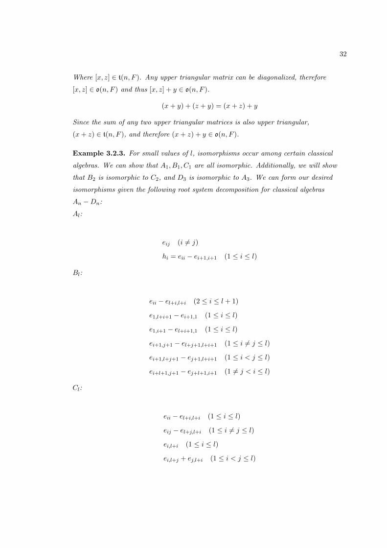
Example 3.2.3. For small values of l, isomorphisms occur among certain classical
algebras. We can show that A1, B1, C1 are all isomorphic. Additionally, we will show
that B2 is isomorphic to C2, and D3 is isomorphic to A3. We can form our desired
isomorphisms given the following root system decomposition for classical algebras
An −Dn:
Al:
eij (i 6= j)
hi = eii − ei+1,i+1 (1 ≤ i ≤ l)
Bl:
eii − el+i,l+i (2 ≤ i ≤ l + 1)
e1,l+i+1 − ei+1,1 (1 ≤ i ≤ l)
e1,i+1 − el+i+1,1 (1 ≤ i ≤ l)
ei+1,j+1 − el+j+1,l+i+1 (1 ≤ i 6= j ≤ l)
ei+1,l+j+1 − ej+1,l+i+1 (1 ≤ i < j ≤ l)
ei+l+1,j+1 − ej+l+1,i+1 (1 6= j < i ≤ l)
Cl:
eii − el+i,l+i (1 ≤ i ≤ l)
eij − el+j,l+i (1 ≤ i 6= j ≤ l)
ei,l+i (1 ≤ i ≤ l)
ei,l+j + ej,l+i (1 ≤ i < j ≤ l)
33
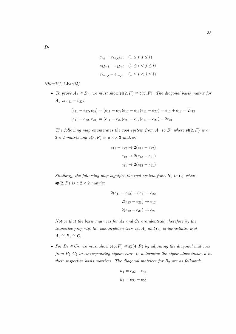
Dl
ei,j − el+j,l+i (1 ≤ i, j ≤ l)
ei,l+j − ej,l+i (1 ≤ i < j ≤ l)
el+i,j − el+j,i (1 ≤ i < j ≤ l)
[Hum72], [Wan75]
• To prove A1∼= B1, we must show sl(2, F ) ∼= o(3, F ). The diagonal basis matrix for
A1 is e11 − e22:
[e11 − e22, e12] = (e11 − e22)e12 − e12(e11 − e22) = e12 + e12 = 2e12
[e11 − e22, e21] = (e11 − e22)e21 − e12(e11 − e21)− 2e21
The following map enumerates the root system from A1 to B1 where sl(2, F ) is a
2× 2 matrix and o(3, F ) is a 3× 3 matrix:
e11 − e22 → 2(e11 − e22)
e12 → 2(e13 − e21)
e21 → 2(e12 − e31)
Similarly, the following map signifies the root system from B1 to C1 where
sp(2, F ) is a 2× 2 matrix:
2(e11 − e22)→ e11 − e22
2(e13 − e21)→ e12
2(e12 − e31)→ e21
Notice that the basis matrices for A1 and C1 are identical, therefore by the
transitive property, the isomorphism between A1 and C1 is immediate. and
A1∼= B1
∼= C1
• For B2∼= C2, we must show o(5, F ) ∼= sp(4, F ) by adjoining the diagonal matrices
from B2, C2 to corresponding eigenvectors to determine the eigenvalues involved in
their respective basis matrices. The diagonal matrices for B2 are as followed:
h1 = e22 − e44
h2 = e33 − e55

34
Denote λ1 = [h1, x] and λ2 = [h2, x], where x is an eigenvector, then eigenvalue
λ = (λ1, λ2). Recall that [hi, x] = −[hi, xt]
[h1, e21 − e14] = h1(e21 − e14)− (e21 − e14)h1
= (e22 − e44)(e21 − e14)− (e21 − e14)(e22 − e44) = e21 − e14 = 1
[h2, e21 − e14] = (e33 − e55)(e21 − e14)− (e21 − e14)(e33 − e55) = 0
[h1, e12 − e41] = e41 − e12 = −1
[h2, e21 − e14] = 0
Therefore, the eigenvalue for eigenvector e21 − e14 is (1, 0) = α, and the eigenvalue
for eigenvector e12 − e41 is (−1, 0) = −α. The remaining eigenvalues are derived
similarly:
λ1 = [h1, x] λ2 = [h2, x] λ = (λ1, λ2)
[h1, e14 − e21] = 1 [h2, e14 − e21] = 0 α = (1, 0)
[h1, e12 − e41] = −1 [h2, e12 − e41] = 0 −α = (−1, 0)
[h1, e32 − e45] = −1 [h2, e32 − e45] = 1 β = (−1, 1)
[h1, e23 − e54] = 1 [h2, e23 − e54] = −1 −β = (1,−1)
[h1, e15 − e31] = 0 [h2, e15 − e31] = 1 α+ β = (1, 0) + (−1, 1) = (0, 1)
[h1, e51 − e13] = 0 [h2, e51 − e13] = −1 −(α+ β) = (−1, 0) + (1,−1) = (0,−1)
[h1, e25 − e34] = 1 [h2, e25 − e34] = 1 2α+ β = 2(1, 0) + (−1, 1) = (1, 1)
[h1, e52 − e43] = −1 [h2, e52 − e43] = −1 −(2α+ β) = −[2(1, 0) + (−1, 1)] = (−1,−1)
Figure 3.2: Table of eigenvalues for B2
The diagonal matrices for C2 are as followed, where l = 2:
h′1 = e11 − e33, h′2 = e22 − e44
Denote λ′1 as the eigenvalue of [h′1, x] and λ′2 as the eigenvalue of [h′2, x] where x is
an eigenvector. Then eigenvalue λ′ = (λ′1, λ′2).

35
λ′1 λ′2 λ′ = (λ′1, λ′2)
[h′1, e21 − e34] = −1 [h′2, e21 − e34] = 1 α′ = (−1, 1)
[h′1, e12 − e43] = 1 [h′2, e12 − e43] = −1 −α′ = (1,−1)
[h′1, e13] = 2 [h′2, e13] = 0 β′ = (2, 0)
[h′1, e31] = −2 [h′2, e31] = 0 −β′ = (−2, 0)
[h′1, e14 + e23] = 1 [h′2, e14 + e23] = 1 α′ + β′ = (−1, 1) + (2, 0) = (1, 1)
[h′1, e41 + e32] = −1 [h′2, e41 + e32] = −1 −(α′ + β′) = −[(−1, 1) + (2, 0)] = (−1,−1)
[h′1, e51 − e13] = 0 [h′2, e51 − e13] = −1 −(α′ + β′) = (−1, 0) + (1,−1) = (0,−1)
[h′1, e24] = 0 [h′2, e24] = 2 2α′ + β′ = 2(−1, 1) + (2, 0) = (0, 2)
[h′1, e42] = 0 [h′2, e42] = −2 −(2α′ + β′) = −[2(−1, 1) + (2, 0)] = (0,−2)
Figure 3.3: Table of eigenvalues for C2
We can construct a linear transformation, where
H ′1 = −1
2h′1 +
1
2h′2 H ′2 =
1
2h1 +
1
2h2
Let the isomorphism between B2 and C2 be defined by the following map:
α(hi) = α′H ′i 1 ≤ i ≤ 2 β(hi) = β′H ′i 1 ≤ i ≤ 2
Therefore, B2∼= C2, where:
e22 − e44 7→ −12(e11 − e33) + 1
2(e22 − e44)e33 − e55 7→ 1
2(e11 − e33) + 12(e22 − e44)
e21 − e14 7→√22 (e21 − e34)
e12 − e41 7→√22 (e12 − e43)
e32 − e45 7→ e13
e23 − e54 7→ e31
e15 − e31 7→√22 (e14 + e23)
e31 − e41 7→√22 (e41 + e32)
e25 − e34 7→ e24
e43 − e52 7→ e42
• For A3∼= D3, we must show sl(4, F ) ∼= o(6, F ). The diagonal matrices for A3 are:
h1 = e11 − e22, h2 = e22 − e33, h3 = e33 − e44
36
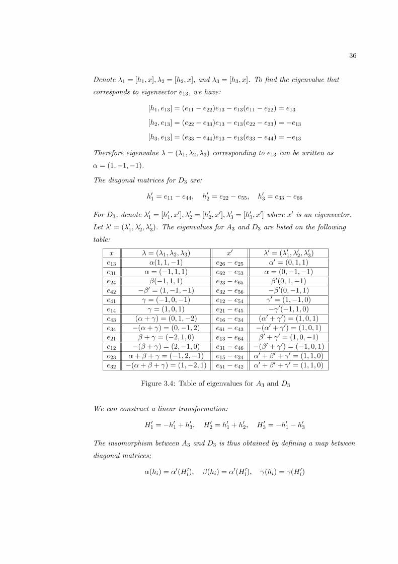
Denote λ1 = [h1, x], λ2 = [h2, x], and λ3 = [h3, x]. To find the eigenvalue that
corresponds to eigenvector e13, we have:
[h1, e13] = (e11 − e22)e13 − e13(e11 − e22) = e13
[h2, e13] = (e22 − e33)e13 − e13(e22 − e33) = −e13
[h3, e13] = (e33 − e44)e13 − e13(e33 − e44) = −e13
Therefore eigenvalue λ = (λ1, λ2, λ3) corresponding to e13 can be written as
α = (1,−1,−1).
The diagonal matrices for D3 are:
h′1 = e11 − e44, h′2 = e22 − e55, h′3 = e33 − e66
For D3, denote λ′1 = [h′1, x′], λ′2 = [h′2, x
′], λ′3 = [h′3, x′] where x′ is an eigenvector.
Let λ′ = (λ′1, λ′2, λ′3). The eigenvalues for A3 and D3 are listed on the following
table:
x λ = (λ1, λ2, λ3) x′ λ′ = (λ′1, λ′2, λ′3)
e13 α(1, 1,−1) e26 − e25 α′ = (0, 1, 1)
e31 α = (−1, 1, 1) e62 − e53 α = (0,−1,−1)
e24 β(−1, 1, 1) e23 − e65 β′(0, 1,−1)
e42 −β′ = (1,−1,−1) e32 − e56 −β′(0,−1, 1)
e41 γ = (−1, 0,−1) e12 − e54 γ′ = (1,−1, 0)
e14 γ = (1, 0, 1) e21 − e45 −γ′(−1, 1, 0)
e43 (α+ γ) = (0, 1,−2) e16 − e34 (α′ + γ′) = (1, 0, 1)
e34 −(α+ γ) = (0,−1, 2) e61 − e43 −(α′ + γ′) = (1, 0, 1)
e21 β + γ = (−2, 1, 0) e13 − e64 β′ + γ′ = (1, 0,−1)
e12 −(β + γ) = (2,−1, 0) e31 − e46 −(β′ + γ′) = (−1, 0, 1)
e23 α+ β + γ = (−1, 2,−1) e15 − e24 α′ + β′ + γ′ = (1, 1, 0)
e32 −(α+ β + γ) = (1,−2, 1) e51 − e42 α′ + β′ + γ′ = (1, 1, 0)
Figure 3.4: Table of eigenvalues for A3 and D3
We can construct a linear transformation:
H ′1 = −h′1 + h′3, H ′2 = h′1 + h′2, H ′3 = −h′1 − h′3
The insomorphism between A3 and D3 is thus obtained by defining a map between
diagonal matrices;
α(hi) = α′(H ′i), β(hi) = α′(H ′i), γ(hi) = γ(H ′i)

37
Therefore A3∼= D3, where:
e11 − e22 7→ −(e11 − e44) + (e33 − e66)e22 − e33 7→ (e11 − e44) + (e22 − e55)e33 − e44 7→ −(e11 − e44)− (e33 − e66)e13 7→ e26 − e25e31 7→ e62 − e53e24 7→ e23 − e65e42 7→ e32 − e56e41 7→ e12 − e54e14 7→ e21 − e45e43 7→ e16 − e34e34 7→ e61 − e43e21 7→ e13 − e64e12 7→ e31 − e46e23 7→ e15 − e24e32 7→ e51 − e42
3.3 Automorphisms
The set of inner automorphisms of a ring, or associative algebra A, is given by the
conjugation element, using right conjugation, such that:
ϕa : A→ A
ϕa(x) = a−1xa
Given x, y ∈ A:
ϕa(xy) = a−1(xy)a = a−1xaa−1ya = (a−1xa)(a−1ya) = ϕa(x)ϕa(y)
Where, ϕa is an (invertible) homomorphism that contains ϕ−1a . Therefore ϕa constitutes
an isomorphism onto itself. Since the composition of conjugation is associative, a−1xa is
often denoted as xa.
Definition 3.12. An automorphism of L is an isomorphism of L onto itself. Aut L
denotes the group of all such.

38
Example 3.3.1. Consider L ⊆ gl(V ), and g ∈ gl(V ) where g is an invertible
endomorphism. Define a mapping φ : L→ L′ where xLx−1 = L, then x→ gxg−1, where
φ is an automophism of L. The same can be said for sl(V ) since the trace of a matrix is
invariant under a change of basis.
Example 3.3.2. Let L be a Lie algebra such that L = sl(n, F ), g ∈ GL(n, F ). The map
ϕ : L→ L defined by x→ −gxtg−1(xt = the transpose of x) belongs to Aut L. When
n = 2, g = the identity matrix, we can prove that Aut L is inner.
tr(−gxtg−1) = tr(−gg−1xt) = tr(−xt) = −tr(x) {Since g = the identity matrix}
⇒tr(x) = 0⇔ tr(−gxtg−1) = 0
Therefore, the map is a linear automorphism of sl(n, F ). If we apply the transpose to
the commutator, for x, y ∈ L, we have:
[x, y]t = (xy − yx)t = (xy)t − (yx)t
= ytxt − xtyt = [ytxt]
Therefore:
ϕ[x, y] = −g[x, y]tg−1 = −g[yt, xt]g−1 {By properties of the transpose}
= g(ytxt − xtyt)g−1 = gytxtg−1 − gxtytg−1
= [gytg−1, gxtg−1] = gytg−1gxtg−1 − gxtg−1gytg−1
= [ϕ(x), ϕ(y)]
Therefore, ϕ is a homomorphism. Thus Aut L is inner.
Example 3.3.3. An automorphism of the form exp(adx), with adx nilpotent, i.e.,
(adx)k = 0 for some k > 1, is called inner.
To derive the power series expansion for exp(adx), we begin by constructing the Taylor
series expansion using the differential operator for matrix A. Given an invertible matrix
A, the solution to x′ = A~x might be x′(t) = λveλt. Multiplying by A, we have:
Ax(t) = Aveλt
where Ax(t) = x′(t)⇔ λv = Av
39
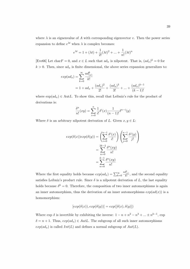
where λ is an eignenvalue of A with corresponding eigenvector v. Then the power series
expansion to define eλt when λ is complex becomes:
eλt = 1 + (λt) +1
2!(λt)2 + ...+
1
n!(λt)n
[Eve66] Let charF = 0, and x ∈ L such that adx is nilpotent. That is, (adx)k = 0 for
k > 0. Then, since adx is finite dimensional, the above series expansion generalizes to:
exp(adx) =∞∑k=0
adk(x)
k!
= 1 + adx +(adx)2
2!+
(adx)3
3!+ ...+
(adx)k−1
(k − 1)!
where exp(adx) ∈ AutL. To show this, recall that Leibniz’s rule for the product of
derivations is:
δn
n!(xy) =
n∑i=0
1
i!δi(x)
1
(n− 1)!δn−i(y)
Where δ is an arbitrary nilpotent derivation of L. Given x, y ∈ L:
exp(δ(x))exp(δ(y)) =
(n−1∑i=0
δi(x)
i!
)n−1∑j=0
δj(y)
j!
=
2k−2∑n=0
δn(xy)
n!
=k−1∑n=0
δn(xy)
n!
Where the first equality holds because exp(adx) =∑∞
k=0
adk(x)
k! , and the second equality
satisfies Leibniz’s product rule. Since δ is a nilpotent derivation of L, the last equality
holds because δk = 0. Therefore, the composition of two inner automorphisms is again
an inner automorphism, thus the derivation of an inner automorphisms exp(ad(x)) is a
homomorphism:
[exp(δ(x)), exp(δ(y))] = exp([δ(x), δ(y)])
Where exp δ is invertible by exhibiting the inverse: 1− n+ n2 − n3 + ...± nk−1, exp
δ = n+ 1. Thus, exp(adx) ∈ AutL. The subgroup of all such inner automorphisms
exp(adx) is called Int(L) and defines a normal subgroup of Aut(L).
40
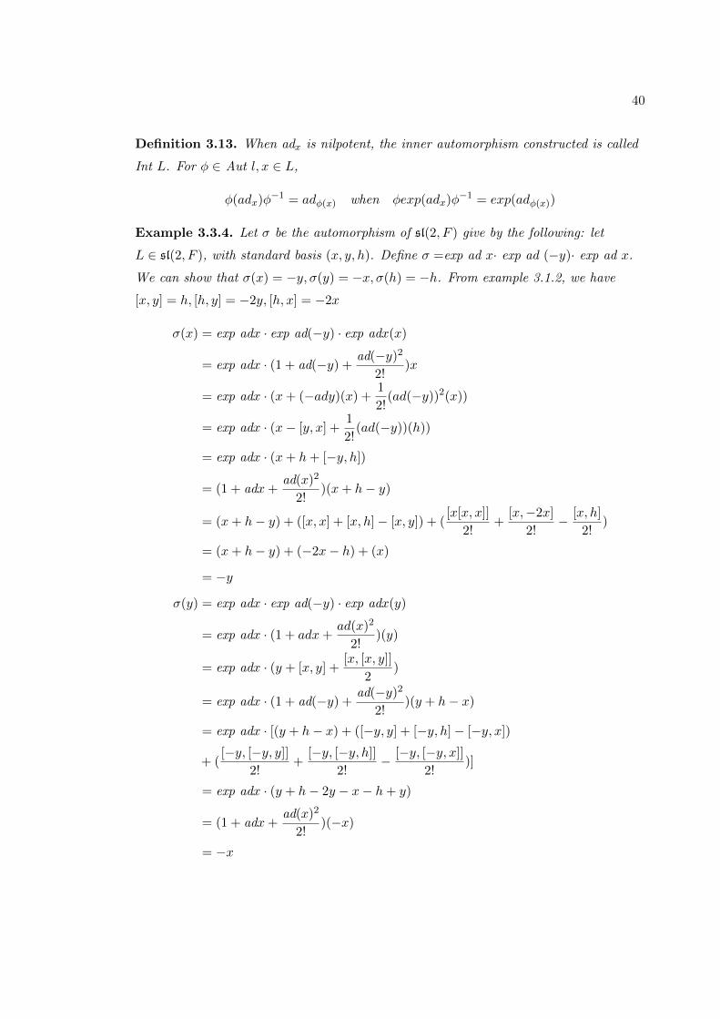
Definition 3.13. When adx is nilpotent, the inner automorphism constructed is called
Int L. For φ ∈ Aut l, x ∈ L,
φ(adx)φ−1 = adφ(x) when φexp(adx)φ−1 = exp(adφ(x))
Example 3.3.4. Let σ be the automorphism of sl(2, F ) give by the following: let
L ∈ sl(2, F ), with standard basis (x, y, h). Define σ =exp ad x· exp ad (−y)· exp ad x.
We can show that σ(x) = −y, σ(y) = −x, σ(h) = −h. From example 3.1.2, we have
[x, y] = h, [h, y] = −2y, [h, x] = −2x
σ(x) = exp adx · exp ad(−y) · exp adx(x)
= exp adx · (1 + ad(−y) +ad(−y)2
2!)x
= exp adx · (x+ (−ady)(x) +1
2!(ad(−y))2(x))
= exp adx · (x− [y, x] +1
2!(ad(−y))(h))
= exp adx · (x+ h+ [−y, h])
= (1 + adx+ad(x)2
2!)(x+ h− y)
= (x+ h− y) + ([x, x] + [x, h]− [x, y]) + ([x[x, x]]
2!+
[x,−2x]
2!− [x, h]
2!)
= (x+ h− y) + (−2x− h) + (x)
= −y
σ(y) = exp adx · exp ad(−y) · exp adx(y)
= exp adx · (1 + adx+ad(x)2
2!)(y)
= exp adx · (y + [x, y] +[x, [x, y]]
2)
= exp adx · (1 + ad(−y) +ad(−y)2
2!)(y + h− x)
= exp adx · [(y + h− x) + ([−y, y] + [−y, h]− [−y, x])
+ ([−y, [−y, y]]
2!+
[−y, [−y, h]]
2!− [−y, [−y, x]]
2!)]
= exp adx · (y + h− 2y − x− h+ y)
= (1 + adx+ad(x)2
2!)(−x)
= −x
41
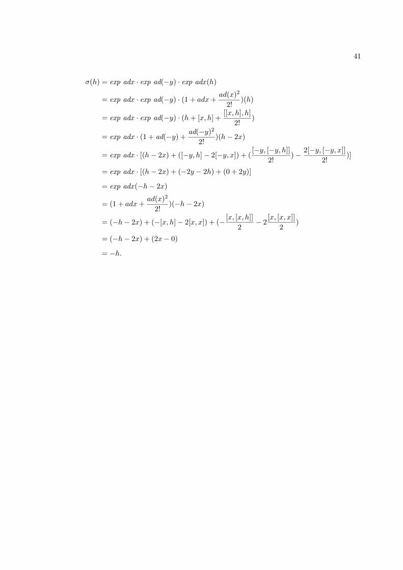
σ(h) = exp adx · exp ad(−y) · exp adx(h)
= exp adx · exp ad(−y) · (1 + adx+ad(x)2
2!)(h)
= exp adx · exp ad(−y) · (h+ [x, h] +[[x, h], h]
2!)
= exp adx · (1 + ad(−y) +ad(−y)2
2!)(h− 2x)
= exp adx · [(h− 2x) + ([−y, h]− 2[−y, x]) + ([−y, [−y, h]]
2!)− 2[−y, [−y, x]]
2!)]
= exp adx · [(h− 2x) + (−2y − 2h) + (0 + 2y)]
= exp adx(−h− 2x)
= (1 + adx+ad(x)2
2!)(−h− 2x)
= (−h− 2x) + (−[x, h]− 2[x, x]) + (− [x, [x, h]]
2− 2
[x, [x, x]]
2)
= (−h− 2x) + (2x− 0)
= −h.
42
Chapter 4
Solvable and Nilpotent Lie
Algebras
4.1 Solvability
In this section, we will decompose L into a collection of subalgebras. Given L as the
direct sum of ideals, the derivation of Li for i = 1, 2...n, consists of a mapping such that
the commutator [Li, Li] is zero.
Definition 4.1. The derived series of a Lie algebra L is a sequence of ideals of L where
L0 = L,L1 = [LL], L2 = [L1L1], ..., Li = [Li−1Li−1].
Given a Lie algebra L, and an ideal I, we have:
[L, I1] = [L, [I, I]] ⊆ [I, [I, L]] + [I, [L, I]] ⊆ [I, I] + [I, I] = I1 [Wan75]
Therefore, if I is an ideal of L, then so is I1. Unless otherwise stated, the material for
this chapter is derived from [Hum72].
Example 4.1.1. Given I is an ideal of L, we can show In+1 is an ideal of L using
induction.
Proof. Since I is an ideal of L, I0 = I is also an ideal of L, as is I1 by the above.
Assume In is an ideal of L. Let x ∈ L, y, z ∈ In.

43
[x[yz]] = −[y[zx]]− [z[xy]] {By the Jacobi identity}
∈ [y, In] + [z, In] {Since [z, x], [x, y] ∈ In}
∈ [In, In] + [In, In] {Since y, z ∈ In}
∈ In+1 + In+1
∈ In+1
Therefore In+1 is an ideal, making each member of the derived series of I an ideal of
L.
Definition 4.2. A group G is said to be solvable if it has a subnormal series
G = G0 ≥ G1 ≥ G2 ≥ ... ≥ Gn = e (4.1)
in which the factors Gi/Gi+1 are all Abelian for all i, 0 ≤ i ≤ n− 1.
By subnormal, we mean that for each i, 0 ≤ i ≤ n− 1, Gi is normal in Gi+1. Given a
Lie algebra L, and series length n > 0 we say that L is solvable if L(n) = 0, that is, a Lie
algebra is solvable if its derived series terminates in the zero subalgebra. The derived
subalgebra of a finite dimensional solvable Lie algebra over a field of characteristic 0 is
nilpotent, thus making abelian algebras solvable and conversely simple algebras
nonsolvable.
Lemma 4.3. Let 0→ J → L→ I → 0 be an exact sequence of Lie algebras. Then L is
solvable if and only if both J and I are solvable. [Sam90]
Proposition 4.4.
1. If L is a solvable Lie algebra, then so are all of the subalgebras and homomorphic
images of L.
2. If I is a solvable ideal of L such that the quotient L/I is solvable, then L itself is
solvable.
3. If I, J are solvable ideals of L, where L is a solvable Lie algebrra, then I + J is
solvable.

44
Proof.
1. Let K be a subalgebra of L, then by definition, K(i) ⊂ L(i), therefore K(i) is
solvable for all i. If we define a map ϕ : L→M where ϕ is an epimorphism, then
by induction, we can show ϕ(L(i)) = M (i).
2. Let (L/I)(n) = 0. By construction of the canonical homomorphism π : L→ LI , we
have that π(L(n)) = 0 by part 1. or L(n) ⊂ I = kerπ. If I(m) = 0, then
(L(i))(i) = L(i+j) ⇒ L(n+m) = 0 (since L(n) ⊂ I).
3. By Proposition 3.11 (part 3.): if I, J are ideals of L, then from the sequence
0→ I → I + J → I+JJ → 0, there exists a natural isomorphism between the third
term (I + J)/J and I/(I ∩ J). Now (I + J)/J is solvable by the Lemma 4.3, since
the homomorphic image of I is solvable. Therefore I/(I ∩ J) is solvable by part 2.
As a consequence of Proposition 4.4, if L is solvable, then L possesses a unique maximal
solvable ideal, called the radical of L, or Rad L. When L is semisimple, Rad L = 0.
Recall, L is simple if it contains no non trivial ideals (i.e., only contains the trivial ideals,
0 and L itself), that is, if Rad L = 0. Therefore, every simple algebra is semisimple.
Example 4.1.2. L is solvable if and only if there exists a chain of subalgebras
L = L0 ⊃ L1 ⊃ ... ⊃ Lk = 0 such that:
• Li+1 is an ideal of Li.
• Each quotient LiLi+1
is abelian.
Proof.
⇒
• Since L is solvable, there exists a sequence of ideals of L such that
L ⊇ L(1) ⊇ ... ⊇ L(i) = 0 for some i. By definition, each ideal forms a subalgebra
of L. By Proposition 4.4, L(i+1) ⊆ L(i) where L(i+1) and L(i) are ideals of L.
• Since L(i+1) is an ideal of L(i) ⊆ L, L(i+1) is an ideal of L. Since L is solvable,
then by definition of the subnormal series, we can show each quotient L(i)
L(i+1) is
45
abelian. By definition of the derived series, L(i+1) = [L(i), L(i)]. Let [x, y] ∈ L(i+1),
with x, y ∈ L(i):
[x+ L(i+1), y + L(i+1)] = [x, y] + [x, L(i+1)] + [L(i+1), y] + [L(i+1), L(i+1)]
= [x, y] + L(i+1)
Therefore L(i)
L(i+1) is abelian.
⇐ Given L(k−1)
L(k) is abelian and L = L0 ⊃ L1 ⊃ ... ⊃ Lk = 0, then the derived series for L
terminates in the zero subalgebra. Therefore, by defintion, Lk is solvable, making L(k−1)
L(k)
solvable, and thus Lk−1 is solvable by Proposition 4.4. Similarly,Lk−2
Lk−1is solvable, and
thus Lk−2 is solvable. Continuing this way, L0L1
is abelian and thus L1 is solvable.
Therefore L0 = L is solvable.
Example 4.1.3. We can show that L is solvable if and only if adL is solvable.
Proof.
⇒ Let L(n) = 0. By induction, when n = 0, L(0) = L, and adL(0) = adL = (adL)(0).
Therefore adL is solvable for n = 0. Assume adL(n) = (adL)(n),
adL(n+1) = ad[L(n), L(n)] {By definition of the derived series}
= [(adL)(n), (adL)(n)]{
Since ad[xy] = [adx, ady]}
= (adL)(n+1){
Since Ln+1 = [Ln, Ln]}
Therefore adL is solvable.
⇐ Since adL is solvable, (adL)(n) = ad(n)L = 0, by the induction above. Therefore
L(n) ⊆ Z(L). Therefore LZ(L) is solvable and thus L is solvable.
4.2 Nilpotency
In this section, we shall explore the descending central series, defined as a recursive
sequence of subalgebras that ends in the zero subspace. We shall rewrite this series
using the quotient space to determine the effect of having a nilpotent algebra as it
relates to it’s subalgebras and their homomorphic images.

46
Definition 4.5. The descending central series is a sequence of ideals of L defined
as L0 = L,L1 = [LL], L2 = [LL1], ..., Li = [LLi−1]. We call L nilpotent if for some
n > 0, Ln = 0.
Thus Li is spanned by long brackets [X1[X2[...XI+1]...] (which we abbreviate to
[X1X2...Xi+1]) [Sam90]. Notice that Ln = 0 makes any abelian algebra nilpotent.
Therefore nilpotent implies solvable since L(i) ⊂ Li for all i. However solvable does not
imply nilpotent.
Example 4.2.1. The algebra n(n, F ) of strictly upper triangular matrices is nilpotent.
A matrix is strictly upper triangular if and only if i > j − k. So Given Bkij = 0, implies
Bk = 0 for k ≥ m if B is an m×m matrix. Using induction, we have B1 = 0 for
i.j − 1. Assume Bkij = 0 for i, j − (k − 1):
Bkij = BBk−1
j =
i∑r=1
BirBk−1rj +
m∑r=i+1
BirBk−1rj
=
i∑r=1
0 ·Bk−1rj +
m∑r=i+1
Bir · 0 = 0
Note that the first term goes to zero, since r ≤ i where Bir is strictly triangular. The
second term goes to zero since r ≥ i+ 1 > (j − k) + 1 = j − (k − 1). Therefore, by the
induction step, Bkij = 0.
We can show a similar result for lower triangular matrices using the following indices:
m ≥ j.i ≥ 1 Cij = Dij = 0
m ≥ i ≥ 1 Cii = Dii = 0
Which would prove that (CD)ij = 0 [Eve66]
Proposition 4.6.
1. If L is a nilpotent Lie algebra, then all the subalgebras and homomorphic images
of L are nilpotent.
2. If L is a Lie algebra such that L/Z(L) is nilpotent, then L is nilpotent.
3. If L 6= 0 is a nilpotent Lie algebra, then Z(L) 6= 0
Proof.
47
1. Let K be a subalgebra, then by definition Ki ⊂ Li. Similarly, if ϕ : L→M is an
epimorphism, we can show, by induction on i, that ϕ(Li) = M i
2. Let Ln ⊂ Z(L), then
Ln+1 = [L,Ln] {By definition of the descending central series}
= [L,Z(L)] = 0 {By definition of the center}
3. If L is nilpotent, Ln = {0}, and Ln−1 6= {0}. By definition of the descending
central series, Ln−1 = [L,Ln], which implies that Ln−1 ⊆ Z(L). Therefore
Z(L) 6= 0.
Example 4.2.2. Let I be an ideal of L. Then each member of the descending central
series of I is also an ideal of L.
Proof. Since I is an ideal of L, I0 = I is also an ideal of L. Assume In = [I, In−1] is an
ideal of L. Let x ∈ L, y ∈ I, z ∈ In.
[x[yz]] = −[y[zx]]− [z[xy]] {By the Jacobi identity}
∈ [y, In] + [z, I] {Since [z, x] ∈ In, [x, y] ∈ I}
∈ [I, In] + [In, I] {Since y ∈ I, z ∈ In}
= In+1 + In+1
= In+1
Therefore In+1 is an ideal, then each member of the descending central series of I is an
ideal of L.
Example 4.2.3. We can show that L is nilpotent if and only if adL is nilpotent.
Proof. Using induction, let n = 0, then L0 = L. Therefore adL0 = (adL)0 = adL. Let
adLn = (adL)n. Then
adLn+1 = [adL, adLn ] {By definition of the descending central series}
= [adL, (adL)n] {Since adLn = (adL)n}
= (adL)n+1

48
⇒ Let Ln = 0 for some n. By the above induction, adLn = (adL)n = 0 and thus adL is
nilpotent.
⇐ Given adL is nilpotent, (adL)n = 0. Since (adL)n = adLn = 0, Ln = 0, therefore L is
nilpotent.
Example 4.2.4. The sum of two nilpotent ideals of a Lie algebra L is again a nilpotent
ideal. Therefore, L possesses a unique maximal nilpotent ideal.
Proof. Let I, J be nilpotent ideals of L. By definition, Im, Jn = 0 for some m,n. Let
n ≥ m. Let x ∈ I, y ∈ J , then:
[x+ y, x+ y] = [x, x] + [x, y] + [y, x] + [y, y]
⊆ [I, I] + [I, J ] + [J, I] + [J, J ]
= [I, I] + [J, J ] + [I, J ]
⊆ [I, I] + [J, J ] + I ∩ J = [I + J, I + J ] [Sam90]
Assume by induction, (I + J)k ⊆ In + Jm + I ∩ J . Our aim is to show the there exists a
k such that (I + J)k = 0 where (I + J)k = [I + J, (I + J)k−1], by definition of the
descending central series. Let k = n+m, by the use of binomial expansion:
(I + J)k = (I + J)n+m = In+m + In+m−1J + ...+ IJn+m−1 + Jn+m
= 0 + In+m−1J + ...+ IJn+m−1 + 0 {Since In, Jm = 0} .
⊆ Ik ∩ J + J ∩ Ik
where (I + J)k = (I + J)n+m = 0. Thus I + J is a nilpotent ideal.
Example 4.2.5. Let charF = 2. We can prove that L = sl(2, F ) is nilpotent. Recall the
standard basis for L:
x =
1 0
0 −1
, y =
0 1
0 0
, z =
0 0
1 0
[x, z] = [(e11 − e22), e21] = (e11 − e22)(e21)− (e21)(e11 − e22) = −e21 − e21 = −2e21 = −2z
[x, y] = [(e11 − e22), e12] = (e11 − e22)(e12)− (e12)(e11 − e22) = e12 − (−e12) = 2e12 = 2y
[y, z] = [e12, e21] = e12e21 − e21e12 = e11 − e22 = x

49
Therefore, by definition of the lower central series,
L1 = [sl(2, F ), sl(2, F )] =
0 −2y 2z
2y 0 −x−2z x 0
Recall [x, x] = 0. Since charF = 2, then [x, z] = 0 = [x, y], and
[sl(2, F ), sl(2, F )] =
0 0 0
0 0 −x0 x 0
= Fx. Therefore by the Jacobi relation,
L2 = [sl(2, F ), [sl(2, F ), sl(2, F )]] = [sl(2, F ), Fx] = 0.
4.3 Proof of Engel’s Theorem
The purpose of Engel’s Theorem is to connect the property of Lie algebra nilpotence to
operators on a vector space. A Lie algebra is nilpotent if for a sufficiently long sequence
{xi} of elements of L, the nested adjoint ad(xn)[...ad(x2)[ad(x1)[y]]] is zero for all y ∈ L.
That is, applying the adjoint sufficiently many times will kill any element belonging to
L, rending each x ∈ L ad-nilpotent. Engel’s theorem states the converse as true. In
preparation for Engel’s theorem, we must first observe the following lemma, then prove
Theorem 4.8.
Lemma 4.7. Let A be a nilpotent operator on a vector space V , then
1. There exists a non-zero v ∈ V such that Av = 0.
2. adA is a nilpotent operator on gl(v).
Theorem 4.8. Let L be a subalgebra of gl(v), with V finite dimensional. If L consists
of nilpotent endomorphisms and V 6= 0, then there exists a nonzero v ∈ V for which
L.v = 0.
Proof. Using induction on dimL. If dim L = 0, then clearly L.v = 0 and the theorem is
true. If dim L = 1, then recall that a single nilpotent linear transformation contains at
least one eigenvector corresponding to eigenvalue 0, thus the theorem is true and
L.v = 0.
50
Given L is a nilpotent Lie algebra, L(n) = 0 for all x1, ..., xn, x ∈ L. Let adx ∈ gl(L)
with x ∈ L ad-nilpotent, then:
[x1, [x2,[...[xn,x]...] = 0
⇔ (adx1)(adx2)...(adxn)(x) = 0
⇔ (adL)n = 0
[GG78]
Suppose K 6= L is any nontrivial subalgebra of L. Consider the vector spaces of K and
L. Since K is a subalgebra of a nilpotent endomorphism, adk(l +K) = adk(l) +K is a
well defined map where, for k′ ∈ K:
adk(l + k′ +K) = adk(l) + adk(k′) +K
= adk(l) +K
Thus adk induces a nilpotent linear transformation on the quotient subspace L/K.
Since K is a subalgebra of L, dimK < dimL. From the induction assumption and
Lemma 4.7, it follows that there exists some non-zero vector x+ k 6= k in L/K such that
x+ k is killed by the image in gl(L/K). By definition, NL(K) = {x ∈ L|[x, k] ⊂ K},therefore K is properly in the normalizer of K in L since for x ∈ L, y ∈ K, [x, y] ⊂ Kwhere x /∈ K. Let K be a maximal proper subalgebra of L, then every x ∈ L has
[x, k] ∈ K for all k ∈ K, which makes NL(K) an ideal of L. Consider the dimension of
L/K. If dimL/K > 1, then there exists a 1 dimensional subalgebra Fv/K ⊆ L/K. By
the correspondance theorem, K ⊆ Fv ⊆ L, but L is not one dimensional. Therefore, K
has codimension 1, which makes L/K one dimensional. Since L/K is 1-dimensional,
Span{l ∈ L} = F (z + L)K for some nilpotent endomorphism z ∈ L. For each l ∈ L,
l +K = αz +K, k ∈ K. Therefore αz ∈ K, and thus l = αz + k for z ∈ l − k.
By induction, W = {v ∈ V |k.v = 0} 6= 0. By the above, K is an ideal of L. If
x ∈ L, y ∈ K,w ∈ V , then since yx− xy = −[x, y] in End (V ), we have:
51
(yx) · w − (xy) · w = −[x, y] · w
(yx) · w = (xy) · w − [x, y] · w
= x(y(w))− 0 · w {since [x, y] is an ideal of K}
= x · 0 {since (y(w)) = 0, y ∈ K}
= 0
Since z is a nilpotent endomorphism in L, L stabilizes W , therefore, z : W →W is
nilpotent. For zn = 0 (zn−1 6= 0), there exists a u ∈ V such that zn−1u 6= 0. Let
v0 = zn−1u ∈W . Then zv0 = zn = 0, Thus, there exists an eigenvector v0 ∈W (v 6= 0)
for which K(vo) = 0. Therefore, L.v = 0 since L = K + Fz.
Theorem 4.9. Engel I Let V be a vector space; let L be a sub Lie algebra of the
general linear Lie algebra gl(V ), consisting entirely of nilpotent operators. Then L is a
nilpotent Lie algebra.
Proof. By Theorem 4.8, if we apply the dual representation (inverse transpose) of L on
V t; the operators are nilpotent. Let λ 6= 0 be a function on V that is anulled by L, then
the space (L · v) spanned by all Xv with X ∈ L, is a proper subspace of V , and in fact,
is in the kernal of λ where λ(Xv) = Xtλ(v) = 0. Recall (L · v) is invariant under L, so
we can iterate the argument. Let m = dimV , then the abbreviated iteration
X1 ·X2...Xm, vanishes, since for every Xi, the dimension of V is decreased by at least 1
where any long bracket [X1X2...Xk] expands by the bracket operation into a sum of
products of kX’s. [Sam90]
Theorem 4.10. Engel II If all elements of L are ad-nilpotent, then L is nilpotent.
Proof. Given a Lie algebra of L having only ad-nilpotent elements, since the adoint is a
linear transformation, adL ⊂ gl(L), which satisfies the hypothesis of Theorem 4.8 when
L 6= 0. Thus there exists an x ∈ L such that [L, x] = 0, which implies that the center of
L is nonzero. Therefore L/Z(L) consists of ad-nilpotent elements, where dim
adL/Z(L) < dimL. Using an induction argument on the dimension of L, similar to
Theorem 4.8, it follows that L/Z(L) is nilpotent. Therefore, by Proposition 4.6 (part
2.), if L/Z(L) is nilpotent, then so is L.
52
Corollary 4.11. Let L be nilpotent, and K be an ideal of L. Then if
k 6= 0, k ∩ Z(L) 6= 0
Proof. Since K is an ideal of L, L induces a linear transfomation on K via the adjoint
representation, therefore there exists x ∈ K(k 6= 0). Therefore [L, x] = 0 by definition of
nilpotency, and thus x ∈ K ∩ Z(L) as desired.

53
Chapter 5
Conclusion
Now that we have covered the basics, we can further explore the root system of the
classical Lie algebras. The full set of roots of a Lie algebra L can be generated from the
set of simple roots and their associated Weyl reflections. If we further explore nilpotent
subalgebras of a Lie algebra that are self-normalising, we invariably must investigate
cartan subalgebras and the killing form.
Differentiating a Lie group action yeids a Lie algebra action. A Lie algebra is a
linearization of a Lie group action, and allows one a doorway to study Lie groups. The
foundation of Lie theory is the exponential map relating Lie algebras to Lie groups,
known as the Lie group-Lie algebra correspondence. We briefly touched on this map
earlier in section 3.3, dealing with Lie algebra automorphisms.
The question arises: what real world applications do Lie algebras possess? Classical
Lie algebra representations have applications in physics. They can be used to study
fluid dynamics. Symmetries in physics take on the structure of mathematical groups,
where continuous groups represent Lie groups. Collisions of vector bosons in quantum
field theory is tied to Lie algebra, specifically gauge theory, and as such, becomes a
mechanism to interpolate physical interactions. The algebra can be promoted to a
group and interpreted as a symmetry (gauge symmetry). Lie algebras are thus integral
to describing theories of nature.

54
Bibliography
[Aig02] Papantonopoulou Aigli. Algebra Pure and Applied. Prentice Hall, New Jersey,
2002.
[Eve66] Howard Eves. Elementary Matrix Theory. Dover Publications, Inc, New York,
1966.
[FIS03] Stephen H. Friedberg, Arnold J. Insel, and Lawrence E. Spence. Linear
Algebra. Pearson Education, Inc, New Jersey, 2003.
[Gal04] Joseph A. Gallian. Contemporary Abstract Algebra. Cengage Learning, New
York, 2004.
[GG78] Morikuni Goto and Frank D. Grosshans. Semisimple Lie Algebras. Marcel
Dekker, Inc, New York, NY, 1978.
[Hum72] James E. Humphreys. Introduction to Lie Algebras and Representation
Theory. Springer-Verlag, New York, 1972.
[MT03] Jerrold E. Marsden and Anthony J. Tromba. Vector Calculus. Wiley, New
York, NY, 2003.
[Sam90] Hans Samelson. Notes on Lie Algebras. Springer-Verlag, New York, 1990.
[Wan75] Zhe-Xian Wan. Lie Algebra. Pergamon Press, Oxford, 1975.