an introduction to graphing utilities - cengage€¦ · appendix a an introduction to graphing...
TRANSCRIPT

APPENDIX A An Introduction to Graphing Utilities A1
Graphing utilities such as graphing calculators and computers with graphing software are very valuable tools for visualizing mathematical principles,verifying solutions to equations, exploring mathematical ideas, and developingmathematical models. Although graphing utilities are extremely helpful in learning mathematics, their use does not mean that learning algebra is any lessimportant. In fact, the combination of knowledge of mathematics and the use ofgraphing utilities enables you to explore mathematics more easily and to a greaterdepth. If you are using a graphing utility in this course, it is up to you to learn its capabilities and to practice using this tool to enhance your mathematical learning.
In this text, there are many opportunities to use a graphing utility, some ofwhich are described below.
In this appendix, the features of graphing utilities are discussed from a generic perspective. To learn how to use the features of a specific graphing utility, consult your user’s manual or the website for this text, found atcollege.hmco.com/info/larsonapplied, where you will find specific keystrokes formost graphing utilities. Your college library may also have a video on how to useyour graphing utility.
The Equation Editor
Many graphing utilities are designed to act as “function graphers.” In this course,functions and their graphs are studied in detail. A function can be thought of as arule that describes the relationship between two variables. These rules are frequently written in terms of x and y. For example, the equation represents y as a function of x.
Many graphing utilities have an equation editor that requires that an equationbe written in “ ” form in order to be entered, as shown in Figure A.1. (You should note that your equation editor screen may not look like the screen shownin Figure A.1.)
y �
y � 3x � 5
A An Introduction to Graphing Utilities
Uses of a Graphing Utility
A graphing utility can be used to
• check or validate answers to problems obtained using algebraic methods.
• discover and explore algebraic properties, rules, and concepts.
• graph functions and approximate solutions of equations involving functions.
• efficiently perform complicated mathematical procedures such as thosefound in many real-life applications.
• find mathematical models for sets of data.
FIGURE A.1
1053715_App_A.qxp 11/5/08 1:29 PM Page A1
A2 APPENDIX A An Introduction to Graphing Utilities
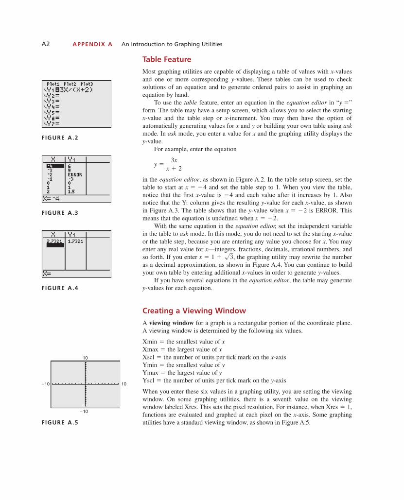
Table Feature
Most graphing utilities are capable of displaying a table of values with x-valuesand one or more corresponding y-values. These tables can be used to check solutions of an equation and to generate ordered pairs to assist in graphing anequation by hand.
To use the table feature, enter an equation in the equation editor in “ ”form. The table may have a setup screen, which allows you to select the startingx-value and the table step or x-increment. You may then have the option of automatically generating values for x and y or building your own table using askmode. In ask mode, you enter a value for x and the graphing utility displays they-value.
For example, enter the equation
in the equation editor, as shown in Figure A.2. In the table setup screen, set thetable to start at and set the table step to 1. When you view the table,notice that the first x-value is and each value after it increases by 1. Alsonotice that the column gives the resulting y-value for each x-value, as shownin Figure A.3. The table shows that the y-value when is ERROR. Thismeans that the equation is undefined when
With the same equation in the equation editor, set the independent variablein the table to ask mode. In this mode, you do not need to set the starting x-valueor the table step, because you are entering any value you choose for x. You mayenter any real value for x—integers, fractions, decimals, irrational numbers, andso forth. If you enter the graphing utility may rewrite the numberas a decimal approximation, as shown in Figure A.4. You can continue to buildyour own table by entering additional x-values in order to generate y-values.
If you have several equations in the equation editor, the table may generate y-values for each equation.
Creating a Viewing Window
A viewing window for a graph is a rectangular portion of the coordinate plane.A viewing window is determined by the following six values.
Xmin the smallest value of xXmax the largest value of xXscl the number of units per tick mark on the x-axisYmin the smallest value of Ymax the largest value of Yscl the number of units per tick mark on the y-axis
When you enter these six values in a graphing utility, you are setting the viewingwindow. On some graphing utilities, there is a seventh value on the viewing window labeled Xres. This sets the pixel resolution. For instance, when Xres 1,functions are evaluated and graphed at each pixel on the x-axis. Some graphingutilities have a standard viewing window, as shown in Figure A.5.
�
�y�y�
���
x � 1 � �3,
x � �2.x � �2
Y1
�4x � �4
y �3x
x � 2
y �
FIGURE A.2
FIGURE A.3
FIGURE A.4
10−10
−10
10
FIGURE A.5
1053715_App_A.qxp 11/5/08 1:29 PM Page A2

By choosing different viewing windows for a graph, it is possible to obtainvery different impressions of the graph’s shape. For instance, Figure A.6 showsfour different viewing windows for the graph of
Of these, the view shown in part (a) is the most complete.
(a) (b)
(c) (d)
FIGURE A.6
On most graphing utilities, the display screen is two-thirds as high as it iswide. On such screens, you can obtain a graph with a true geometric perspectiveby using a square setting—one in which
One such setting is shown in Figure A.7. Notice that the x and y tick marks areequally spaced on a square setting, but not on a standard setting.
To see how the viewing window affects the geometric perspective, graph thesemicircles using a standard viewing window. Then graph and using a square viewing window. Note the differencein the shapes of the circles.
Zoom and Trace Features
When you graph an equation, you can move from point to point along its graphusing the trace feature. As you trace the graph, the coordinates of each point aredisplayed, as shown in Figure A.8. The trace feature combined with the zoomfeature enables you to obtain better and better approximations of desired pointson a graph.
For instance, you can use the zoom feature of a graphing utility to approx-imate the x-intercept(s) of a graph. Suppose you want to approximate the
y2y1
y1 � �9 � x2 and y2 � ��9 � x2
Ymax � YminXmax � Xmin
�23
.
11
−2
−1 10
y = 0.1x4 − x3 + 2x22
−8
6−4
y = 0.1x4 − x3 + 2x2
10
10−5
−10
y = 0.1x4 − x3 + 2x28
−16
−8 16
y = 0.1x4 − x3 + 2x2
y � 0.1x 4 � x3 � 2x2.
−4
6−6
4
FIGURE A.7
−6 6
4
−4
FIGURE A.8
APPENDIX A An Introduction to Graphing Utilities A3
1053715_App_A.qxp 11/5/08 1:29 PM Page A3
A4 APPENDIX A An Introduction to Graphing Utilities
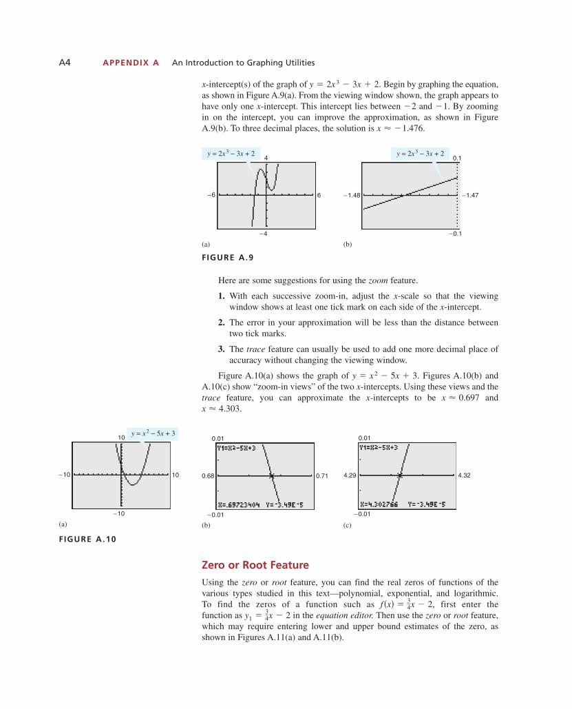
x-intercept(s) of the graph of Begin by graphing the equation,as shown in Figure A.9(a). From the viewing window shown, the graph appears tohave only one x-intercept. This intercept lies between and By zoomingin on the intercept, you can improve the approximation, as shown in FigureA.9(b). To three decimal places, the solution is
(a) (b)
FIGURE A.9
Here are some suggestions for using the zoom feature.
1. With each successive zoom-in, adjust the x-scale so that the viewing window shows at least one tick mark on each side of the x-intercept.
2. The error in your approximation will be less than the distance betweentwo tick marks.
3. The trace feature can usually be used to add one more decimal place ofaccuracy without changing the viewing window.
Figure A.10(a) shows the graph of Figures A.10(b) andA.10(c) show “zoom-in views” of the two x-intercepts. Using these views and thetrace feature, you can approximate the x-intercepts to be and
(b) (c)
Zero or Root Feature
Using the zero or root feature, you can find the real zeros of functions of the various types studied in this text—polynomial, exponential, and logarithmic. To find the zeros of a function such as first enter the function as in the equation editor. Then use the zero or root feature,which may require entering lower and upper bound estimates of the zero, asshown in Figures A.11(a) and A.11(b).
y1 �34x � 2
f�x� �34x � 2,
−0.01
4.29 4.32
0.01
−0.01
0.68 0.71
0.01
x � 4.303.x � 0.697
y � x2 � 5x � 3.
0.1
−0.1
−1.48 −1.47
y = 2x3 − 3x + 24
6
−4
−6
y = 2x3 − 3x + 2
x � �1.476.
�1.�2
y � 2x3 � 3x � 2.
10
10
−10
−10
y = x2 − 5x + 3
(a)
FIGURE A.10
1053715_App_A.qxp 11/5/08 1:29 PM Page A4

In Figure A.11(c), you can see that the zero is
Intersect Feature
To find the point(s) of intersection of two graphs, you can use the intersectfeature. For instance, to find the point(s) of intersection of the graphs of
and
enter these two functions in the equation editor and use the intersect feature, asshown in Figure A.12.
(a) (b)
(c) (d)
FIGURE A.12
From Figure A.12(d), you can see that the point of intersection is ��1, 3�.
6
4−8
−2
y1 = −x + 2
y2 = x + 4
6
4−8
−2
y1 = −x + 2
y2 = x + 4
6
4−8
−2
y1 = −x + 2
y2 = x + 4
6
4−8
−2
y1 = −x + 2
y2 = x + 4
y2 � x � 4y1 � �x � 2
x � 2.6666667 � 223.
10−10
−10
10
(a)
FIGURE A.11
10
−10
−10
10
(b)
10
10
−10
−10
f (x) = 34 x − 2
(c)
APPENDIX A An Introduction to Graphing Utilities A5
1053715_App_A.qxp 11/5/08 1:29 PM Page A5
A6 APPENDIX A An Introduction to Graphing Utilities
Regression Feature
Throughout the text, you are asked to use the regression feature of a graphing utility to find models for sets of data. Most graphing utilities have built-in regression programs for the following.
Regression Form of Model
Linear or
Quadratic
Cubic
Quartic
Logarithmic
Exponential
Power
Logistic
Sine
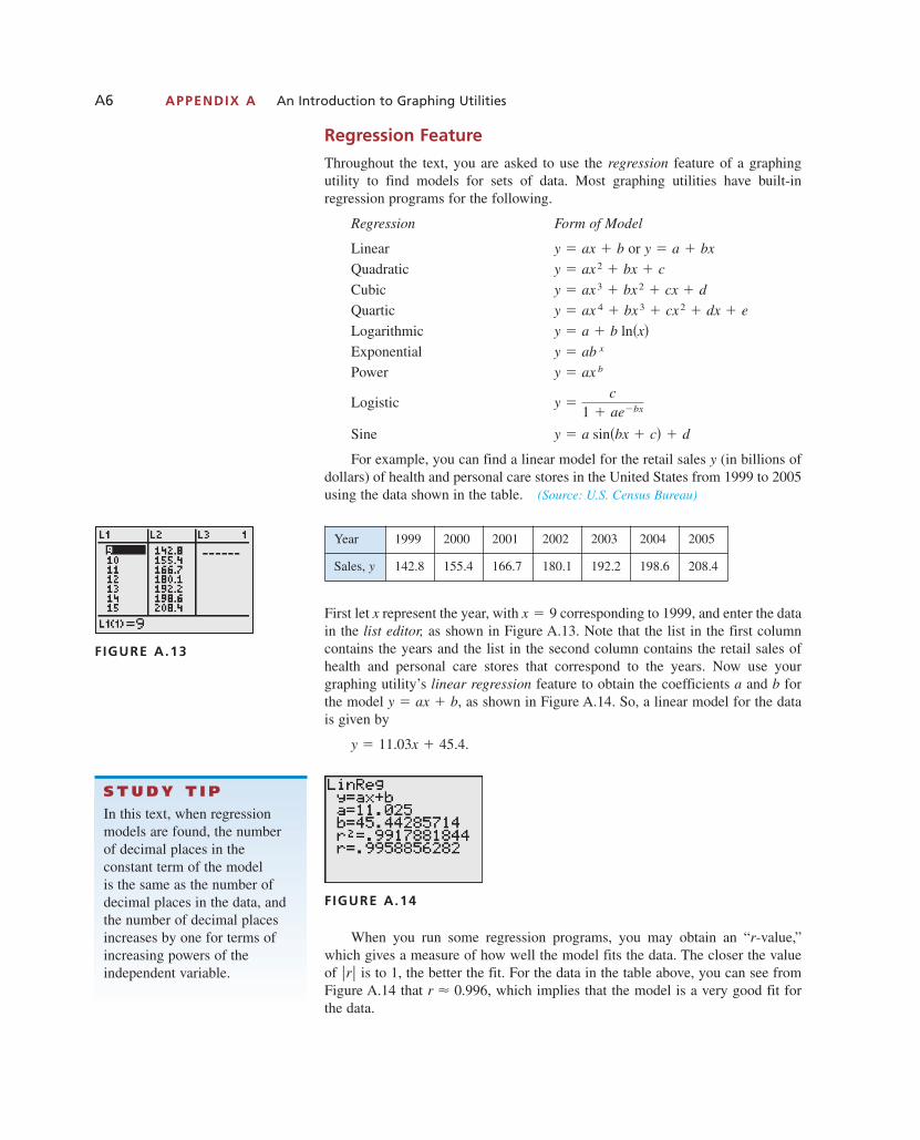
For example, you can find a linear model for the retail sales (in billions ofdollars) of health and personal care stores in the United States from 1999 to 2005using the data shown in the table. (Source: U.S. Census Bureau)
First let represent the year, with corresponding to 1999, and enter the datain the list editor, as shown in Figure A.13. Note that the list in the first columncontains the years and the list in the second column contains the retail sales ofhealth and personal care stores that correspond to the years. Now use your graphing utility’s linear regression feature to obtain the coefficients and forthe model as shown in Figure A.14. So, a linear model for the datais given by
FIGURE A.14
When you run some regression programs, you may obtain an “r-value,”which gives a measure of how well the model fits the data. The closer the valueof is to 1, the better the fit. For the data in the table above, you can see fromFigure A.14 that which implies that the model is a very good fit forthe data.
r � 0.996,�r�
y � 11.03x � 45.4.
y � ax � b,ba
x � 9x
y
y � a sin�bx � c� � d
y �c
1 � ae�bx
y � ax b
y � ab x
y � a � b ln�x�y � ax 4 � bx3 � cx2 � dx � e
y � ax3 � bx2 � cx � d
y � ax2 � bx � c
y � a � bxy � ax � b
S T U D Y T I PIn this text, when regressionmodels are found, the number of decimal places in the constant term of the model is the same as the number ofdecimal places in the data, andthe number of decimal placesincreases by one for terms ofincreasing powers of the independent variable.
FIGURE A.13
Year 1999 2000 2001 2002 2003 2004 2005
Sales, y 142.8 155.4 166.7 180.1 192.2 198.6 208.4
1053715_App_A.qxp 11/5/08 1:29 PM Page A6
Maximum and Minimum Features
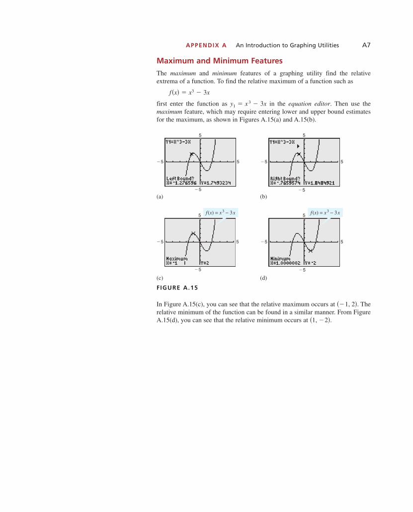
The maximum and minimum features of a graphing utility find the relativeextrema of a function. To find the relative maximum of a function such as
first enter the function as in the equation editor. Then use themaximum feature, which may require entering lower and upper bound estimatesfor the maximum, as shown in Figures A.15(a) and A.15(b).
(a) (b)
(c) (d)
FIGURE A.15
In Figure A.15(c), you can see that the relative maximum occurs at Therelative minimum of the function can be found in a similar manner. From FigureA.15(d), you can see that the relative minimum occurs at �1, �2�.
��1, 2�.
5
5
�5
�5
f (x) = x3 − 3x
5
5
�5
�5
f (x) = x3 − 3x
5�5
�5
5
5�5
�5
5
y1 � x3 � 3x
f�x� � x3 � 3x
APPENDIX A An Introduction to Graphing Utilities A7
1053715_App_A.qxp 11/5/08 1:29 PM Page A7

A8 APPENDIX B Conic Sections
B.1 Conic Sections■ Recognize the four basic conics: circles, parabolas, ellipses, and hyperbolas.
■ Recognize, graph, and write equations of parabolas (vertex at origin).
■ Recognize, graph, and write equations of ellipses (center at origin).
■ Recognize, graph, and write equations of hyperbolas (center at origin).
B Conic Sections
Introduction to Conic Sections
Conic sections were discovered during the classical Greek period, which lastedfrom 600 to 300 B.C. By the beginning of the Alexandrian period, enough wasknown of conics for Apollonius (262–190 B.C.) to produce an eight-volume workon the subject.
This early Greek study was largely concerned with the geometric properties ofconics. It was not until the early seventeenth century that the broad applicability ofconics became apparent.
A conic section (or simply conic) can be described as the intersection of aplane and a double-napped cone. Notice in Figure B.1 that in the formation of thefour basic conics, the intersecting plane does not pass through the vertex of thecone. When the plane does pass through the vertex, the resulting figure is adegenerate conic, as shown in Figure B.2.
There are several ways to approach the study of conics. You could begin by defining conics in terms of the intersections of planes and cones, as the Greeksdid, or you could define them algebraically, in terms of the general second-degreeequation
However, you will study a third approach in which each of the conics is definedas a locus, or collection, of points satisfying a certain geometric property. Forexample, in Section 2.1 you saw how the definition of a circle as the collectionof all points that are equidistant from a fixed point led easily to thestandard equation of a circle, �x � h�2 � �y � k�2 � r 2.
�h, k��x, y�
Ax 2 � Bxy � Cy2 � Dx � Ey � F � 0.
FIGURE B.1 Conic Sections FIGURE B.2 Degenerate Conics
1053715_App_B01.qxp 11/5/08 1:20 PM Page A8

APPENDIX B.1 Conic Sections A9
You will restrict your study of conics in this section to parabolas withvertices at the origin and ellipses and hyperbolas with centers at the origin. In thefollowing section, you will look at the more general cases.
Parabolas
In Section 3.1 you determined that the graph of the quadratic function given by
is a parabola that opens upward or downward. The following definition of aparabola is more general in the sense that it is independent of the orientation ofthe parabola.
Using this definition, you can derive the following standard form of the equation of a parabola.
f�x� � ax2 � bx � c
Definition of a Parabola
A parabola is the set of all points in a plane that are equidistant from afixed line called the directrix and a fixed point called the focus (not on theline). The midpoint between the focus and the directrix is called the vertex,and the line passing through the focus and the vertex is called the axis of the parabola.
x
y
(x, y)
Directrix
Axis
Focus
Vertex
d2
d2d1
d1
�x, y�
Standard Equation of a Parabola (Vertex at Origin)
The standard form of the equation of a parabola with vertex at anddirectrix is given by
Vertical axis
For directrix the equation is given by
Horizontal axis
The focus is on the axis units (directed distance) from the vertex. SeeFigure B.3.
p
y2 � 4px, p � 0.
x � �p,
x2 � 4py, p � 0.
y � �p�0, 0�
S T U D Y T I PNote that the term parabolais a technical term used in mathematics and does not simplyrefer to any U-shaped curve.
Focus (0, p)
x
p
p
y
(x, y)
Axis
x2 = 4py, p ≠ 0
Vertex (0, 0)
Directrix: y = −p
Parabola with vertical axis
x
y
(x, y)
Focus (p, 0)
p p
Vertex(0, 0)
Axis
y2 = 4px, p ≠ 0
Dir
ectr
ix: x
= −
p
Parabola with horizontal axis
FIGURE B.3
1053715_App_B01.qxp 11/5/08 1:20 PM Page A9
A10 APPENDIX B Conic Sections
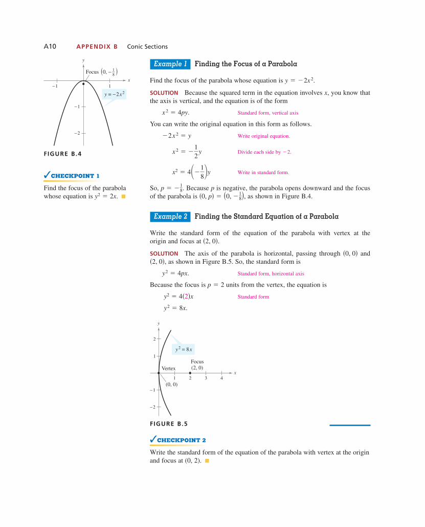
Example 1 Finding the Focus of a Parabola
Find the focus of the parabola whose equation is
SOLUTION Because the squared term in the equation involves you know thatthe axis is vertical, and the equation is of the form
Standard form, vertical axis
You can write the original equation in this form as follows.
Write original equation.
Divide each side by
Write in standard form.
So, Because is negative, the parabola opens downward and the focusof the parabola is as shown in Figure B.4.
Example 2 Finding the Standard Equation of a Parabola
Write the standard form of the equation of the parabola with vertex at theorigin and focus at
SOLUTION The axis of the parabola is horizontal, passing through andas shown in Figure B.5. So, the standard form is
Standard form, horizontal axis
Because the focus is units from the vertex, the equation is
Standard form
FIGURE B.5
✓CHECKPOINT 2
Write the standard form of the equation of the parabola with vertex at the originand focus at (0, 2). ■
x(2, 0)
1
2
y
(0, 0)1 2 3 4
−1
−2
FocusVertex
y2 = 8x
y2 � 8x.
y2 � 4�2�x
p � 2
y2 � 4px.
�2, 0�,�0, 0�
�2, 0�.
�0, p� � �0, �18�,
pp � �18.
x2 � 4��18�y
�2. x2 � �12
y
�2x2 � y
x2 � 4py.
x,
y � �2x2.x1
−
y
Focus 0, 18( (
−1
−1
−2
y = −2x2
FIGURE B.4
✓CHECKPOINT 1
Find the focus of the parabolawhose equation is ■y2 � 2x.
1053715_App_B01.qxp 11/5/08 1:20 PM Page A10
APPENDIX B.1 Conic Sections A11
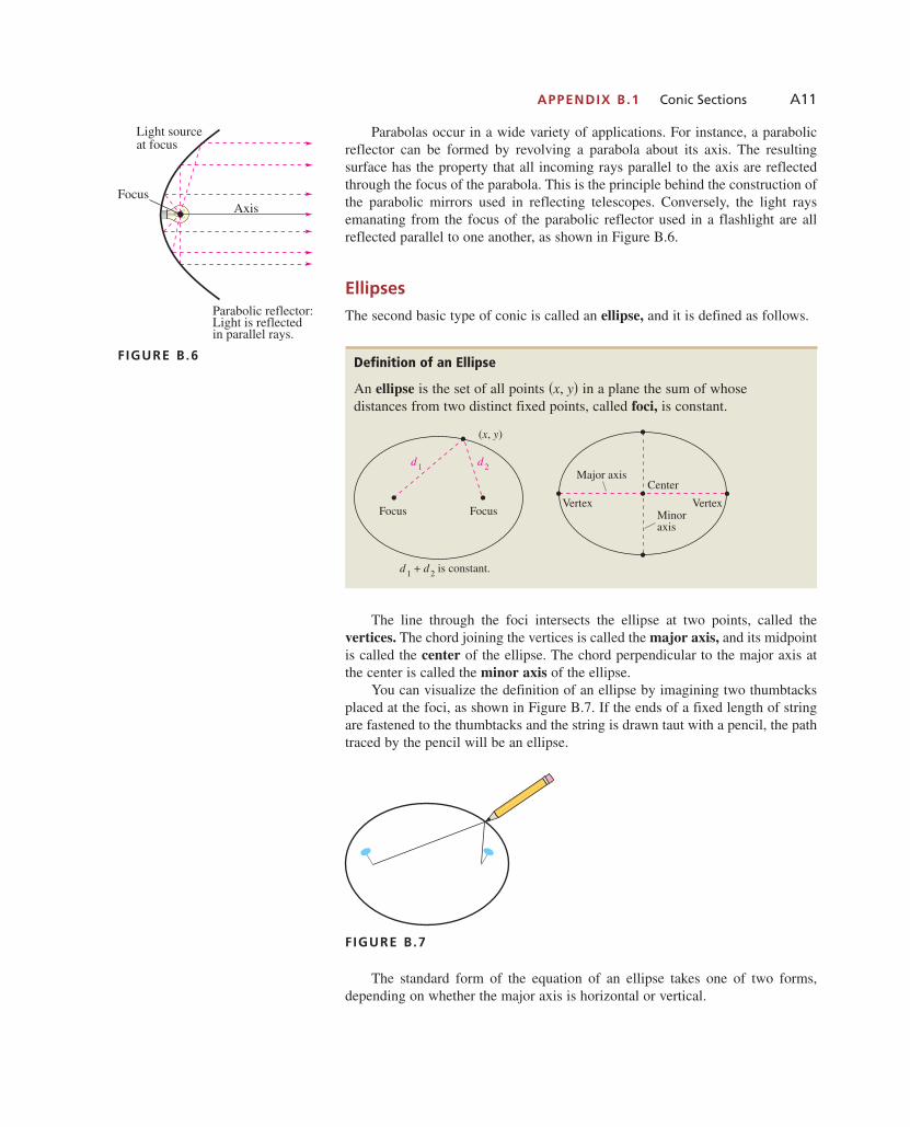
Parabolas occur in a wide variety of applications. For instance, a parabolicreflector can be formed by revolving a parabola about its axis. The resultingsurface has the property that all incoming rays parallel to the axis are reflectedthrough the focus of the parabola. This is the principle behind the construction ofthe parabolic mirrors used in reflecting telescopes. Conversely, the light raysemanating from the focus of the parabolic reflector used in a flashlight are allreflected parallel to one another, as shown in Figure B.6.
Ellipses
The second basic type of conic is called an ellipse, and it is defined as follows.
The line through the foci intersects the ellipse at two points, called thevertices. The chord joining the vertices is called the major axis, and its midpointis called the center of the ellipse. The chord perpendicular to the major axis atthe center is called the minor axis of the ellipse.
You can visualize the definition of an ellipse by imagining two thumbtacksplaced at the foci, as shown in Figure B.7. If the ends of a fixed length of stringare fastened to the thumbtacks and the string is drawn taut with a pencil, the pathtraced by the pencil will be an ellipse.
FIGURE B.7
The standard form of the equation of an ellipse takes one of two forms,depending on whether the major axis is horizontal or vertical.
Definition of an Ellipse
An ellipse is the set of all points in a plane the sum of whose distances from two distinct fixed points, called foci, is constant.
Center
VertexVertex
Major axis
Minoraxis
Focus Focus
d1 + d2 is constant.
d1 d2
(x, y)
�x, y�
Axis
Light sourceat focus
Focus
Parabolic reflector:Light is reflectedin parallel rays.
FIGURE B.6
1053715_App_B01.qxp 11/5/08 1:20 PM Page A11

A12 APPENDIX B Conic Sections
Example 3 Finding the Standard Equation of an Ellipse
Find the standard form of the equation of the ellipse that has a major axis oflength 6 and foci at and as shown in Figure B.8.
SOLUTION Because the foci occur at and the center of the ellipseis and the major axis is horizontal. So, the ellipse has an equation of the form
Standard form, horizontal major axis
Because the length of the major axis is 6, you have which implies thatMoreover, the distance from the center to either focus is Finally,
you have
Substituting and yields the following equation in standardform.
Standard form
This equation simplifies to x 2
9�
y2
5� 1.
x2
32 �y2
��5�2 � 1
b 2 � ��5�2a2 � 32
b2 � a2 � c2 � 32 � 22 � 9 � 4 � 5.
c � 2.a � 3.2a � 6,
x2
a2 �y2
b2 � 1.
�0, 0�,�2, 0�,��2, 0�
�2, 0�,��2, 0�
Standard Equation of an Ellipse (Center at Origin)
The standard form of the equation of an ellipse with the center at the origin and major and minor axes of lengths 2a and 2b (where ) is
or
Major axis is horizontal. Major axis is vertical.Minor axis is vertical. Minor axis is horizontal.
The vertices and foci lie on the major axis, and units, respectively, fromthe center. Moreover, and are related by the equation
c2 � a2 � b2.
cb,a,ca
x
(0, −c)
y
Vertex
Vertex
(−b, 0)
(b, 0)
(0, −a)
(0, c)
(0, a)x2
b2
y2
a2+ = 1
x
(0, )−b
y
Vertex
Vertex
(−c, 0)
(−a, 0)
(c, 0) (a, 0)
(0, b)
x2
a2
y2
b2+ = 1
x2
b2 �y2
a2 � 1.x2
a2 �y2
b2 � 1
0 < b < a
x
1
3
(2, 0)(−2, 0)
y
−1
−1−2
−3
1 2
x2
a2
y2
b2+ = 1
FIGURE B.8
✓CHECKPOINT 3
Find the standard form of the equation of the ellipse that has amajor axis of length 8 and foci at
and ■�0, 3�.�0, �3�
1053715_App_B01.qxp 11/5/08 1:20 PM Page A12

APPENDIX B.1 Conic Sections A13
Example 4 Sketching an Ellipse
Sketch the ellipse given by and identify the vertices.
SOLUTION Begin by writing the equation in standard form.
Write original equation.
Divide each side by 36.
Write in standard form.
Simplify.
Because the denominator of the -term is larger than the denominator of the -term, you can conclude that the major axis is vertical. Moreover, because the vertices are and Finally, because the endpoints of theminor axis are and as shown in Figure B.9.
FIGURE B.9
Note that from the standard form of the equation, you can sketch the ellipseby locating the endpoints of the two axes. Because is the denominator of the
-term, move three units to the right and left of the center to locate the endpointsof the horizontal axis. Similarly, because is the denominator of the -term,move six units upward and downward from the center to locate the endpoints ofthe vertical axis.
✓CHECKPOINT 4
Sketch the ellipse given by and identify the vertices. ■
Hyperbolas
The definition of a hyperbola is similar to that of an ellipse. The distinction isthat, for an ellipse, the sum of the distances between the foci and a point on theellipse is constant, whereas for a hyperbola, the difference of the distancesbetween the foci and a point on the hyperbola is constant.
x2 � 4y2 � 64,
y262x2
32
x
2
4
(3, 0)(−3, 0)
(0, 6)
(0, −6)
y
−2
−2
−4
−4−6 2 4 6
x2
32
y2
62+ = 1
�3, 0�,��3, 0�b � 3,�0, 6�.�0, �6�
a � 6,x2y2
x 2
9�
y2
36� 1
x2
32 �y2
62 � 1
4x2
36�
y2
36�
3636
4x2 � y2 � 36
4x2 � y2 � 36,
S T U D Y T I PThe endpoints of the minor axisof an ellipse are commonlyreferred to as the co-vertices.In Figure B.9, the co-verticesare and �3, 0�.��3, 0�
1053715_App_B01.qxp 11/5/08 1:20 PM Page A13
A14 APPENDIX B Conic Sections
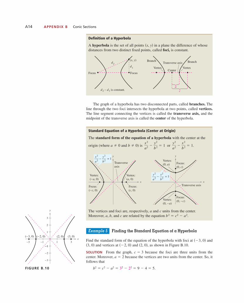
The graph of a hyperbola has two disconnected parts, called branches. Theline through the two foci intersects the hyperbola at two points, called vertices.The line segment connecting the vertices is called the transverse axis, and themidpoint of the transverse axis is called the center of the hyperbola.
Example 5 Finding the Standard Equation of a Hyperbola
Find the standard form of the equation of the hyperbola with foci at andand vertices at and as shown in Figure B.10.
SOLUTION From the graph, because the foci are three units from the center. Moreover, because the vertices are two units from the center. So, itfollows that
b2 � c2 � a2 � 32 � 22 � 9 � 4 � 5.
a � 2c � 3
�2, 0�,��2, 0��3, 0���3, 0�
Standard Equation of a Hyperbola (Center at Origin)
The standard form of the equation of a hyperbola with the center at the
origin (where and ) is or
The vertices and foci are, respectively, a and c units from the center.Moreover, and are related by the equation b2 � c2 � a2.ca, b,
x
Focus:(0, c)
Focus:(0, −c)
Vertex:(0, a)
Vertex:(0, −a)
Transverse axis
y
y2
a2
x2
b2− = 1
x
y
Vertex:(−a, 0)
Vertex:(a, 0)
Focus:(−c, 0)
Focus:(c, 0)
Transverseaxis
x2
a2
y2
b2− = 1
y2
a2 �x2
b2 � 1.x2
a2 �y2
b2 � 1b � 0a � 0
−13 1− 3
1
2
3
−1
x(2, 0) (3, 0)
y
(−3, 0) (−2, 0)
−1
−2
−3
FIGURE B.10
Definition of a Hyperbola
A hyperbola is the set of all points in a plane the difference of whosedistances from two distinct fixed points, called foci, is constant.
ac
Branch Branch
Center
Transverse axis
Vertex Vertex
Focus Focus
(x, y)
d2 − d1 is constant.
d1
d2
�x, y�
1053715_App_B01.qxp 11/5/08 1:20 PM Page A14
APPENDIX B.1 Conic Sections A15
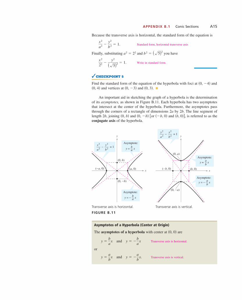
Because the transverse axis is horizontal, the standard form of the equation is
Standard form, horizontal transverse axis
Finally, substituting and you have
Write in standard form.
✓CHECKPOINT 5
Find the standard form of the equation of the hyperbola with foci at andand vertices at and ■
An important aid in sketching the graph of a hyperbola is the determinationof its asymptotes, as shown in Figure B.11. Each hyperbola has two asymptotesthat intersect at the center of the hyperbola. Furthermore, the asymptotes passthrough the corners of a rectangle of dimensions 2a by 2b. The line segment oflength 2b, joining and or and is referred to as theconjugate axis of the hyperbola.
Transverse axis is horizontal. Transverse axis is vertical.
FIGURE B.11
x
y
(−b, 0)
(0, a)
(b, 0)
(0, −a)
Asymptote:
Asymptote:
y = xab
y = − xab
y2
a2
x2
b2− = 1
x
y
(0, −b)
(0, b)
(a, 0)(−a, 0)
x2
a2
y2
b2− = 1
Asymptote:bay = x
Asymptote:bay = − x
�b, 0��,��b, 0���0, �b��0, b�
�0, 3�.�0, �3��0, 4��0, �4�
x2
22 �y2
��5�2 � 1.
b2 � ��5�2a2 � 22
x2
a2 �y2
b2 � 1.
Asymptotes of a Hyperbola (Center at Origin)
The asymptotes of a hyperbola with center at are
and Transverse axis is horizontal.
or
and Transverse axis is vertical.y � �ab
x.y �ab
x
y � �ba
xy �ba
x
�0, 0�
1053715_App_B01.qxp 11/5/08 1:20 PM Page A15

A16 APPENDIX B Conic Sections
Example 6 Sketching a Hyperbola
Sketch the hyperbola whose equation is
SOLUTION
Write original equation.
Divide each side by 16.
Write in standard form.
Because the -term is positive, you can conclude that the transverse axis is horizontal and the vertices occur at and Moreover, the endpointsof the conjugate axis occur at and and you can sketch the rectangle shown in Figure B.12. Finally, by drawing the asymptotes through thecorners of this rectangle, you can complete the sketch shown in Figure B.13.
FIGURE B.12 FIGURE B.13
Example 7 Finding the Standard Equation of a Hyperbola
Find the standard form of the equation of the hyperbola that has vertices at and and asymptotes and as shown in Figure B.14.
SOLUTION Because the transverse axis is vertical, the asymptotes are of the form
and Transverse axis is vertical.
Using the fact that and you can determine that
Because you can determine that Finally, you can conclude that thehyperbola has the following equation.
Write in standard form.
✓CHECKPOINT 7
Find the standard form of the equation of the hyperbola that has vertices atand and asymptotes and ■y � x.y � �x�5, 0���5, 0�
y2
32 �x2
�32�2 � 1
b �32.a � 3,
ab � 2.y � �2x,y � 2x
y � �ab
x. y �ab
x
y � 2x,y � �2x�0, 3��0, �3�
6
x
y
4 6−4−6
−6
x2
22
y2
42− = 1
6
x
(0, 4)
(0, −4)
(2, 0)(−2, 0)
y
−6
−6 −4 4 6
�0, 4�,�0, �4��2, 0�.��2, 0�
x2
x2
22 �y2
42 � 1
4x2
16�
y2
16�
1616
4x2 � y2 � 16
4x2 � y2 � 16.
✓CHECKPOINT 6
Sketch the hyperbola whose equation is ■9y2 � x2 � 9.
x2 4
2
4
(0, 3)
y
y = −2x
y = 2x
(0, −3)−2
−4
−2−4
FIGURE B.14
1053715_App_B01.qxp 11/5/08 1:20 PM Page A16
APPENDIX B.1 Conic Sections A17
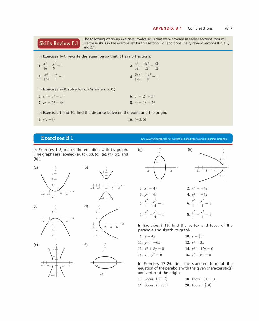
In Exercises 1–8, match the equation with its graph.[The graphs are labeled (a), (b), (c), (d), (e), (f ), (g), and(h).]
(a) (b)
(c) (d)
(e) (f )
(g) (h)
1. 2.
3. 4.
5. 6.
7. 8.
In Exercises 9–16, find the vertex and focus of theparabola and sketch its graph.
9. 10.
11. 12.
13. 14.
15. 16.
In Exercises 17–26, find the standard form of the equation of the parabola with the given characteristic(s)and vertex at the origin.
17. Focus: 18. Focus:
19. Focus: 20. Focus: �52, 0���2, 0�
�0, �2��0, �32�
y2 � 8x � 0x � y2 � 0
x2 � 12y � 0x2 � 8y � 0
y2 � 3xy2 � �6x
y �12x2y � 4x2
y2
4�
x2
1� 1
x2
1�
y2
4� 1
x2
4�
y2
1� 1
x2
1�
y2
4� 1
y2 � �4xy2 � 4x
x2 � �4yx2 � 4y
x
4
y
−12 −8 −4
−4
x
1
2
y
−2
x1
2
y
−1
−2
x2
2
4
4
y
−2−4
−4
x
2
4
y
−2−2
−4
2 64
x
2
4
y
−2
−4
−4
−6
x
4
y
2 4−2−4
−4
x
6
4
2
y
−2−2−4 2 4
Exercises B.1 See www.CalcChat.com for worked-out solutions to odd-numbered exercises.
The following warm-up exercises involve skills that were covered in earlier sections. You willuse these skills in the exercise set for this section. For additional help, review Sections 0.7, 1.3,and 2.1.
In Exercises 1–4, rewrite the equation so that it has no fractions.
1. 2.
3. 4.
In Exercises 5–8, solve for (Assume )
5. 6.
7. 8.
In Exercises 9 and 10, find the distance between the point and the origin.
9. 10. ��2, 0��0, �4�
c2 � 12 � 22c2 � 22 � 42
c2 � 22 � 32c2 � 32 � 12
c > 0.c.
3x2
19�
4y2
9� 1
x2
14�
y2
4� 1
x2
32�
4y2
32�
3232
x2
16�
y2
9� 1
Skills Review B.1
1053715_App_B01.qxp 11/5/08 1:20 PM Page A17

A18 APPENDIX B Conic Sections
21. Directrix:
22. Directrix:
23. Directrix:
24. Directrix:
25. Passes through the point horizontal axis
26. Passes through the point vertical axis
In Exercises 27–34, find the center and vertices of theellipse and sketch its graph.
27. 28.
29. 30.
31. 32.
33. 34.
In Exercises 35–42, find the standard form of theequation of the ellipse with the given characteristicsand center at the origin.
35. Vertices: minor axis of length 2
36. Vertices: minor axis of length 3
37. Vertices: foci:
38. Vertices: foci:
39. Foci: major axis of length 12
40. Foci: major axis of length 8
41. Vertices: passes through the point
42. Major axis vertical; passes through the points and
In Exercises 43–50, find the center and vertices of thehyperbola and sketch its graph.
43. 44.
45. 46.
47. 48.
49. 50.
In Exercises 51–58, find the standard form of the equation of the hyperbola with the given characteristicsand center at the origin.
51. Vertices: foci:
52. Vertices: foci:
53. Vertices: asymptotes:
54. Vertices: asymptotes:
55. Foci: asymptotes:
56. Foci: asymptotes:
57. Vertices: passes through the point
58. Vertices: passes through the point
59. Satellite Antenna The receiver in a parabolictelevision dish antenna is 3 feet from the vertex and islocated at the focus (see figure). Write an equation for across section of the reflector. (Assume that the dish isdirected upward and the vertex is at the origin.)
60. Suspension Bridge Each cable of the Golden GateBridge is suspended (in the shape of a parabola) betweentwo towers that are 1280 meters apart. The top of eachtower is 152 meters above the roadway (see figure). Thecables touch the roadway at the midpoint between the towers.Write an equation for the parabolic shape of each cable.
61. Architecture A fireplace arch is to be constructed in theshape of a semiellipse. The opening is to have a height of 2feet at the center and a width of 5 feet along the base (seefigure). The contractor draws the outline of the ellipse bythe method shown in Figure B.7. Where should the tacks beplaced, and what should be the length of the piece of string?
1
3
x
y
−1−2−3 1 2 3
xRoadway
(640, 152)(−640, 152)
y
Cable
x
3 ftReceiver
y
�3, �3��±2, 0�;��2, 5��0, ±3�;
y � ± 34 x�±10, 0�;
y � ±12x�0, ±4�;
y � ±3x�0, ±3�;y � ±3x�±1, 0�;
�±5, 0��±3, 0�;�0, ±4��0, ±2�;
3y2 � 5x2 � 152x2 � 3y2 � 6
x2
36�
y2
4� 1
y2
25�
x2
144� 1
y2
9�
x2
1� 1
y2
1�
x2
4� 1
x2
9�
y2
16� 1x2 � y2 � 1
�2, 0��0, 4�
�4, 2��0, ±5�;�±2, 0�;�±5, 0�;
�0, ±4��0, ±10�;�±2, 0��±5, 0�;
�±2, 0�;�0, ±2�;
x2 � 4y2 � 45x2 � 3y2 � 15
x2
28�
y2
64� 1
x2
9�
y2
5� 1
x2
4�
y2
14
� 1x2
259
�y2
169
� 1
x2
144�
y2
169� 1
x2
25�
y2
16� 1
��2, �2�;�4, 6�;
x � �2
x � 3
y � 2
y � �1
1053715_App_B01.qxp 11/5/08 1:20 PM Page A18

APPENDIX B.1 Conic Sections A19
62. Mountain Tunnel A semielliptical arch over a tunnelfor a road through a mountain has a major axis of 100 feet,and its height at the center is 30 feet (see figure). Determinethe height of the arch 5 feet from the edge of the tunnel.
63. Sketch a graph of the ellipse that consists of all points such that the sum of the distances between and twofixed points is 15 units and the foci are located at the centers of the two sets of concentric circles, as shown in the figure.
64. Think About It A line segment through a focus of anellipse with endpoints on the ellipse and perpendicular toits major axis is called a latus rectum of the ellipse.Therefore, an ellipse has two latera recta. Knowing thelength of the latera recta is helpful in sketching an ellipsebecause this information yields other points on the curve(see figure). Show that the length of each latus rectum is
In Exercises 65–68, sketch the ellipse using the laterarecta (see Exercise 64).
65.
66.
67.
68.
69. Navigation Long-range navigation for aircraft andships is accomplished by synchronized pulses transmittedby widely separated transmitting stations. These pulsestravel at the speed of light (186,000 miles per second). Thedifference in the times of arrival of these pulses at an aircraft or ship is constant on a hyperbola having the trans-mitting stations as foci. Assume that two stations 300 milesapart are positioned on a rectangular coordinate system atpoints with coordinates and and that aship is traveling on a path with coordinates (see figure). Find the -coordinate of the position of the ship ifthe time difference between the pulses from the transmit-ting stations is 1000 microseconds (0.001 second).
70. Hyperbolic Mirror A hyperbolic mirror (used in sometelescopes) has the property that a light ray directed at onefocus will be reflected to the other focus (see figure). Thefocus of the hyperbolic mirror has coordinates Findthe vertex of the mirror if its mount at the top edge of themirror has coordinates
(12, 0)
(12, 12)
x
y
(−12, 0)
�12, 12�.
�12, 0�.
75 150
150
x
y
−150
x�x, 75�
�150, 0���150, 0�
5x2 � 3y2 � 15
9x2 � 4y2 � 36
x2
9�
y2
16� 1
x2
4�
y2
1� 1
x
Latera recta
y
F2F1
2b2a.
�x, y��x, y�
x30 ft
100 ft45 ft
y
1053715_App_B01.qxp 11/5/08 1:20 PM Page A19

A20 APPENDIX B Conic Sections
B.2 Conic Sections and Translations■ Recognize equations of conics that have been shifted vertically or
horizontally in the plane.
■ Write and graph equations of conics that have been shifted verticallyor horizontally in the plane.
Vertical and Horizontal Shifts of Conics
In Section B.1, you studied conic sections whose graphs were in standardposition. In this section, you will study the equations of conic sections that havebeen shifted vertically or horizontally in the plane. The following summary liststhe standard forms of the equations of the four basic conics.
Standard Forms of Equations of Conics
Circle: Center Radius
Parabola: VertexDirected distance from vertex to focus
x
y
Vertex:(h, k)
Focus:(h + p, k)
(y − k)2 = 4p (x − h)
p > 0
x
y
Focus:(h, k + p)
Vertex:(h, k)
p > 0
(x − h)2 = 4p (y − k)
� p� �h, k�
x
(h, k)r
(x − h)2 + (y − k)2 = r2y
� r� �h, k�;
1053715_App_B02.qxp 11/5/08 1:20 PM Page A20

APPENDIX B.2 Conic Sections and Translations A21
Example 1 Equations of Conic Sections
Describe the translation of the graph of each conic.
a. b.
c. d.
SOLUTION
a. The graph of is a circle whose center is the pointand whose radius is 3, as shown in Figure B.15(a) on the following
page. Note that the graph of the circle has been shifted one unit to the right andtwo units downward from standard position.
b. The graph of is a parabola whose vertex is the pointThe axis of the parabola is vertical. The focus is one unit above or below
the vertex. Moreover, because it follows that the focus lies below thevertex, as shown in Figure B.15(b). Note that the graph of the parabola has beenshifted two units to the right and three units upward from standard position.
p � �1,�2, 3�.
�x � 2�2 � 4��1��y � 3�
�1, �2��x � 1�2 � �y � 2�2 � 32
�x � 2�2
32 ��y � 1�2
22 � 1�x � 3�2
12 ��y � 2�2
32 � 1
�x � 2�2 � 4��1��y � 3��x � 1�2 � �y � 2�2 � 32
Standard Forms of Equations of Conics (continued)
Ellipse: CenterMajor axis length Minor axis length
Hyperbola: CenterTransverse axis length Conjugate axis length
x
y
(h, k)2a
2b
(y − k )2
a2
(x − h )2
b2− = 1
x
y
(h, k)
2a
2b
(x − h)2
a2
(y − k )2
b2− = 1
� 2b� 2a;� �h, k�
x
y (x − h)2
b2
(y − k)2
a2+ = 1
(h, k)2a
2bx
y
2a
2b(h, k)
(x − h)2
a2
(y − k)2
b2+ = 1
� 2b� 2a;� �h, k�
1053715_App_B02.qxp 11/5/08 1:20 PM Page A21

A22 APPENDIX B Conic Sections
c. The graph of
is a hyperbola whose center is the point The transverse axis is horizontal with a length of The conjugate axis is vertical with alength of as shown in Figure B.15(c). Note that the graph of thehyperbola has been shifted three units to the right and two units upward fromstandard position.
d. The graph of
is an ellipse whose center is the point The major axis of the ellipse ishorizontal with a length of The minor axis of the ellipse is verticalwith a length of as shown in Figure B.15(d). Note that the graph ofthe ellipse has been shifted two units to the right and one unit upward fromstandard position.
(a) (b)
(c) (d)
FIGURE B.15
Writing Equations of Conics in Standard Form
To write the equation of a conic in standard form, complete the square, as demonstrated in Examples 2, 3, and 4.
x
4
(2, 1)
3
2
y
+(x − 2)2
32
(y − 1)2
22= 1
−1−1
−2
1 3 5x
(3, 2)3
1
y
6 8 10
2
4
6
8−
(x − 3)2
12
(y − 2)2
32= 1
x
(2, 3)
(2, 2)
31 4 5
1
2
3
4
y
−1−1
−2
p = −1
(x − 2)2 = 4(−1)(y − 3)
(1, −2)
x
3
y
−1
−2
−3
−4
−2−3 1 2 3 4 5
−5
−6
1
2(x − 1)2 + (y + 2)2 = 32
2�2� � 4,2�3� � 6.
�2, 1).
�x � 2�2
32 ��y � 1�2
22 � 1
2�3� � 6,2�1� � 2.
�3, 2�.
�x � 3�2
12 ��y � 2�2
32 � 1
✓CHECKPOINT 1
Describe the translation of thegraph of
■�x � 4�2 � �y � 3�2 � 52.
1053715_App_B02.qxp 11/5/08 1:20 PM Page A22
APPENDIX B.2 Conic Sections and Translations A23
1
2
x
(1, 1)
(1, 0)
y
(x − 1)2 = 4(−1)(y − 1)
−1
−2
−2
−3
−4
1 2 3 4
FIGURE B.16
x
1
2
3
4
y
−1
−1
−2−3−4−5
(−3, 0)
(−3, 1)
(−1, 1)
(−5, 1)(−3, 2)
(x + 3)2
22
(y − 1)2
12+ = 1
FIGURE B.17
✓CHECKPOINT 2
Find the vertex and focus of theparabola given by
■x2 � 2x � 4y � 5 � 0.
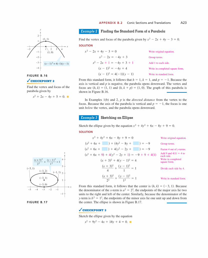
Example 2 Finding the Standard Form of a Parabola
Find the vertex and focus of the parabola given by
SOLUTION
Write original equation.
Group terms.
Add 1 to each side.
Write in completed square form.
Write in standard form.
From this standard form, it follows that and Because theaxis is vertical and p is negative, the parabola opens downward. The vertex andfocus are and The graph of this parabola isshown in Figure B.16.
In Examples 1(b) and 2, p is the directed distance from the vertex to thefocus. Because the axis of the parabola is vertical and the focus is oneunit below the vertex, and the parabola opens downward.
Example 3 Sketching an Ellipse
Sketch the ellipse given by the equation
SOLUTION
Write original equation.
Group terms.
Factor 4 out of y-terms.
Divide each side by 4.
Write in standard form.
From this standard form, it follows that the center is Becausethe denominator of the x-term is the endpoints of the major axis lie twounits to the right and left of the center. Similarly, because the denominator of they-term is the endpoints of the minor axis lie one unit up and down fromthe center. The ellipse is shown in Figure B.17.
✓CHECKPOINT 3
Sketch the ellipse given by the equation
■x2 � 9y2 � 4x � 18y � 4 � 0.
b2 � 12,
a2 � 22,�h, k� � ��3, 1�.
�x � 3�2
22 ��y � 1�2
12 � 1
�x � 3�2
4�
�y � 1�2
1� 1
�x � 3�2 � 4�y � 1�2 � 4
�x2 � 6x � 9� � 4�y2 � 2y � 1� � �9 � 9 � 4�1�
�x2 � 6x � �� � 4�y2 � 2y � �� � �9
�x2 � 6x � �� � �4y2 � 8y � �� � �9
x2 � 4y2 � 6x � 8y � 9 � 0
x2 � 4y2 � 6x � 8y � 9 � 0.
p � �1,
�h, k � p� � �1, 0�.�h, k� � �1, 1�
p � �1.k � 1,h � 1,
�x � 1�2 � 4��1��y � 1�
�x � 1�2 � �4y � 4
x2 � 2x � 1 � �4y � 3 � 1
x2 � 2x � �4y � 3
x2 � 2x � 4y � 3 � 0
x2 � 2x � 4y � 3 � 0.
Add 9 and toeach side.
4�1� � 4
Write in completedsquare form.
1053715_App_B02.qxp 11/5/08 1:20 PM Page A23
A24 APPENDIX B Conic Sections
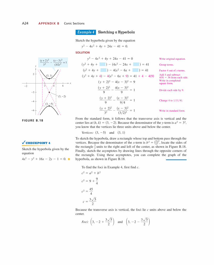
Example 4 Sketching a Hyperbola
Sketch the hyperbola given by the equation
SOLUTION
Write original equation.
Group terms.
Factor 4 out of x-terms.
Divide each side by 9.
Change 4 to
Write in standard form.
From the standard form, it follows that the transverse axis is vertical and the center lies at Because the denominator of the y-term is you know that the vertices lie three units above and below the center.
Vertices: and
To sketch the hyperbola, draw a rectangle whose top and bottom pass through thevertices. Because the denominator of the x-term is locate the sides ofthe rectangle units to the right and left of the center, as shown in Figure B.18.Finally, sketch the asymptotes by drawing lines through the opposite corners ofthe rectangle. Using these asymptotes, you can complete the graph of the hyperbola, as shown in Figure B.18.
To find the foci in Example 4, first find c.
Because the transverse axis is vertical, the foci lie c units above and below thecenter.
Foci: and �3, �2 �3�5
2 ��3, �2 �3�5
2 �
c �3�5
2
c2 �454
c2 � 9 �94
c2 � a2 � b2
32
b2 � �32�2
,
�3, 1��3, �5�
a2 � 32,�h, k� � �3, �2�.
�y � 2�2
32 ��x � 3�2
�3�2�2 � 1
1��1�4�. �y � 2�2
9�
�x � 3�2
9�4� 1
�y � 2�2
9�
4�x � 3�2
9� 1
�y � 2�2 � 4�x � 3�2 � 9
�y2 � 4y � 4� � 4�x2 � 6x � 9� � 41 � 4 � 4�9�
�y2 � 4y � �� � 4�x2 � 6x � �� � 41
�y2 � 4y � �� � �4x2 � 24x � �� � 41
y2 � 4x2 � 4y � 24x � 41 � 0
y2 � 4x2 � 4y � 24x � 41 � 0.
Add 4 and subtractfrom each side.4�9� � 36
Write in completedsquare form.x
y
2 (3, 1)
(y + 2)2
32
(x − 3)2
(3/2)2− = 1
2 4 6
(3, −2)
(3, −5)
−2
−2
−4
−6
FIGURE B.18
✓CHECKPOINT 4
Sketch the hyperbola given by theequation
■4x2 � y2 � 16x � 2y � 1 � 0.
1053715_App_B02.qxp 11/5/08 1:20 PM Page A24

APPENDIX B.2 Conic Sections and Translations A25
Example 5 Writing the Equation of an Ellipse
Write the standard form of the equation of the ellipse whose vertices are and The length of the minor axis of the ellipse is 4, as shown
in Figure B.19.
SOLUTION The center of the ellipse lies at the midpoint of its vertices. So, thecenter is
Center
Because the vertices lie on a vertical line and are six units apart, it follows thatthe major axis is vertical and has a length of So, Moreover,because the minor axis has a length of 4, it follows that which impliesthat Therefore, you can conclude that the standard form of the equation ofthe ellipse is as follows.
Major axis is vertical.
Write in standard form.
✓CHECKPOINT 5
Write the standard form of the equation of the ellipse whose vertices areand The length of the minor axis of the ellipse is 3. ■
An interesting application of conic sections involves the orbits of comets inour solar system. Of the 610 comets identified prior to 1970, 245 have ellipticalorbits, 295 have parabolic orbits, and 70 have hyperbolic orbits. For example,Halley’s comet has an elliptical orbit, and reappearance of this comet can bepredicted every 76 years. The center of the sun is a focus of each of these orbits,and each orbit has a vertex at the point where the comet is closest to the sun, asshown in Figure B.20.
If p is the distance between the vertex and the focus (in meters), and v is thespeed of the comet at the vertex (in meters per second), then the type of orbit isdetermined as follows.
1. Ellipse:
2. Parabola:
3. Hyperbola:
In each of these equations, kilograms (the mass of the sun)and cubic meter per kilogram-second squared (the universalgravitational constant).
G � 6.67 � 10�11M � 1.989 � 1030
v > �2GMp
v ��2GMp
v < �2GMp
�4, 4�.��1, 4�
�x � 2�2
22 ��y � 1�2
32 � 1
�x � h�2
b2 ��y � k�2
a2 � 1
b � 2.2b � 4,
a � 3.2a � 6.
�h, k� � �2 � 22
, 4 � ��2�
2 � � �2, 1�.
�2, 4�.�2, �2�
x
1
2
3
4
4
(2, 4)
y
1 2 3 4 5−1
−1
−2(2, −2)
FIGURE B.19
p
Hyperbolic orbit
Vertex
Sun (Focus)
Elliptical orbit
Parabolic orbit
FIGURE B.20
1053715_App_B02.qxp 11/5/08 1:20 PM Page A25

A26 APPENDIX B Conic Sections
In Exercises 1–6, describe the translation of the graphof the conic from the standard position.
1. 2.
3. 4.
5. 6.
In Exercises 7–16, find the vertex, focus, and directrixof the parabola. Then sketch its graph.
7.
8.
9. 10.
11. 12.
13.
14.
15.
16.
In Exercises 17–24, find the standard form of the equation of the parabola with the given characteristics.
17. Vertex: focus:
18. Vertex: focus:
19. Vertex: directrix:
20. Vertex: directrix:
21. Focus: directrix:
22. Focus: directrix:
23. Vertex: passes through and
24. Vertex: passes through and
In Exercises 25–32, find the center, foci, and vertices ofthe ellipse. Then sketch its graph.
25.�x � 1�2
9�
�y � 5�2
25� 1
�4, 0��0, 0��2, 4�;�2, 0���2, 0��0, 4�;
y � 4�0, 0�;x � �2�2, 2�;
x � 1��2, 1�;y � 2�0, 4�;
��1, 0���1, 2�;�1, 2��3, 2�;
x2 � 2x � 8y � 9 � 0
y2 � 6y � 8x � 25 � 0
y2 � x � y � 0
4x � y2 � 2y � 33 � 0
y � �16 �x2 � 4x � 2�y �
14 �x2 � 2x � 5�
�x �12�2
� 4�y � 3��y �12�2
� 2�x � 5��x � 3� � �y � 2�2 � 0
�x � 1�2 � 8�y � 2� � 0
−2−6 2−2
−4
−6
−8
2
x
y
(x + 2)2
4
(y + 3)2
9− = 1
1 2 3 5−1−2−3
−6
2
x
y
(x − 1)2
9
(y + 2)2
16+ = 1
x
y
1 2 3 4 6
−3−4
1234
(x − 2)2
9
(y + 1)2
4+ = 1
−2 2 4 6−2
−4
−6
x
y
(y + 3)2
4− (x − 1)2 = 1
x
y
−4 4 8 12−4
−8
8
(y − 1)2 = 4(2)(x + 2)
x
y
−4 1−1
1
2
3
4
5
(x + 2)2 + (y − 1)2 = 4
The following warm-up exercises involve skills that were covered in earlier sections. You will usethese skills in the exercise set for this section. For additional help, review Section B.1.
In Exercises 1–12, identify the conic represented by the equation.
1. 2. 3.
4. 5. 6.
7. 8. 9.
10. 11. 12.x2
9�4�
y2
4� 13y2 � 3x2 � 48
9x2
16�
y2
4� 1
3x � y2 � 0x2 � 6y � 0y2
4�
x2
2� 1
4x2 � 4y2 � 25x2
4�
y2
16� 1
x2
9�
y2
4� 1
2x � y2 � 0x2
9�
y2
1� 1
x2
4�
y2
4� 1
Skills Review B.2
Exercises B.2 See www.CalcChat.com for worked-out solutions to odd-numbered exercises.
1053715_App_B02.qxp 11/5/08 1:20 PM Page A26
APPENDIX B.2 Conic Sections and Translations A27
26.
27.
28.
29.
30.
31.
32.
In Exercises 33–42, find the standard form of theequation of the ellipse with the given characteristics.
33. Vertices: minor axis of length 2
34. Vertices: minor axis of length 6
35. Foci: major axis of length 8
36. Foci: major axis of length 16
37. Center: vertex:minor axis of length 2
38. Center: vertex:minor axis of length 6
39. Center: foci:
40. Center: vertices:
41. Vertices: endpoints of minor axis:
42. Vertices: endpoints of minor axis:
In Exercises 43–52, find the center, vertices, and foci ofthe hyperbola. Then sketch its graph, using asymptotesas a sketching aid.
43.
44.
45.
46.
47.
48.
49.
50.
51.
52.
In Exercises 53–60, find the standard form of the equation of the hyperbola with the given characteristics.
53. Vertices: foci:
54. Vertices: foci:
55. Vertices: foci:
56. Vertices: foci:
57. Vertices: passes through
58. Vertices: passes through
59. Vertices:asymptotes:
60. Vertices:asymptotes:
In Exercises 61–68, identify the conic by writing theequation in standard form. Then sketch its graph.
61.
62.
63.
64.
65.
66.
67.
68.
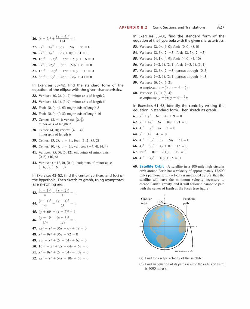
69. Satellite Orbit A satellite in a 100-mile-high circularorbit around Earth has a velocity of approximately 17,500miles per hour. If this velocity is multiplied by then thesatellite will have the minimum velocity necessary toescape Earth’s gravity, and it will follow a parabolic pathwith the center of Earth as the focus (see figure).
(a) Find the escape velocity of the satellite.
(b) Find an equation of its path (assume the radius of Earthis 4000 miles).
x
Circularorbit
Parabolicpath4100
Not drawn to scale
y
�2,
4x2 � 4y2 � 16y � 15 � 0
25x2 � 10x � 200y � 119 � 0
4y2 � 2x2 � 4y � 8x � 15 � 0
4x2 � 3y2 � 8x � 24y � 51 � 0
y2 � 4y � 4x � 0
4x2 � y2 � 4x � 3 � 0
x2 � 4y2 � 6x � 16y � 21 � 0
x2 � y2 � 6x � 4y � 9 � 0
y � 4 �23 xy �
23x,
�3, 0�, �3, 4�;y � 4 �
23 xy �
23x ,
�0, 2�, �6, 2�;�4, 3���2, 1�, �2, 1�;�0, 5��2, 3�, �2, �3�;
��3, 1�, �3, 1���2, 1�, �2, 1�;�4, 0�, �4, 10��4, 1�, �4, 9�;
�2, 5�, �2, �5��2, 3�, �2, �3�;�0, 0�, �8, 0��2, 0�, �6, 0�;
9x2 � y2 � 54x � 10y � 55 � 0
x2 � 9y2 � 2x � 54y � 107 � 0
16y2 � x2 � 2x � 64y � 63 � 0
9y2 � x2 � 2x � 54y � 62 � 0
x2 � 9y2 � 36y � 72 � 0
9x2 � y2 � 36x � 6y � 18 � 0
�y � 1�2
1�4�
�x � 3�2
1�9� 1
�y � 6�2 � �x � 2�2 � 1
�x � 1�2
144�
�y � 4�2
25� 1
�x � 1�2
4�
�y � 2�2
1� 1
��6, 3�, ��6, �3���12, 0�, �0, 0�;
�0, 6�, �10, 6��5, 0�, �5, 12�;
��4, 4�, �4, 4��0, 4�; a � 2c;
�1, 2�, �5, 2��3, 2�; a � 3c;
�4, �4�;�4, 0�;
�2, 12�;�2, �1�;�0, 0�, �0, 8�;�0, 0�, �4, 0�;
�3, 1�, �3, 9�;�0, 2�, �4, 2�;
36x2 � 9y2 � 48x � 36y � 43 � 0
12x2 � 20y2 � 12x � 40y � 37 � 0
9x2 � 25y2 � 36x � 50y � 61 � 0
16x2 � 25y2 � 32x � 50y � 16 � 0
9x2 � 4y2 � 36x � 8y � 31 � 0
9x2 � 4y2 � 36x � 24y � 36 � 0
�x � 2�2 ��y � 4�2
1�4� 1
1053715_App_B02.qxp 11/5/08 1:20 PM Page A27
A28 APPENDIX B Conic Sections
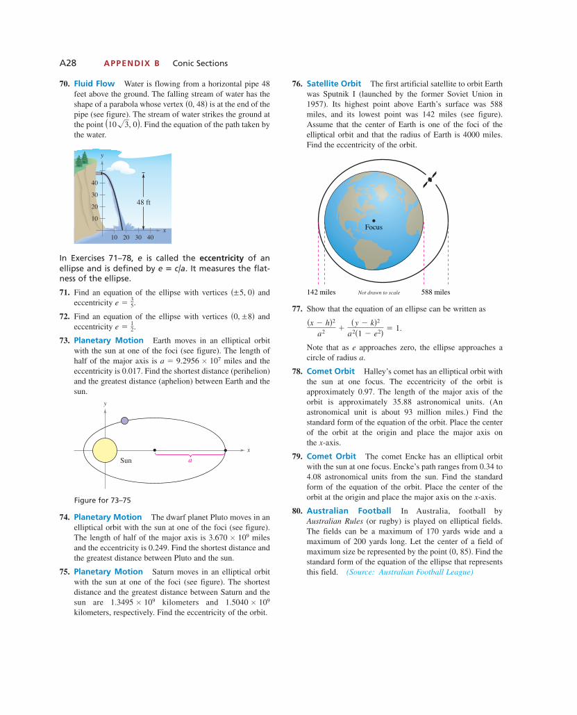
70. Fluid Flow Water is flowing from a horizontal pipe 48feet above the ground. The falling stream of water has theshape of a parabola whose vertex is at the end of thepipe (see figure). The stream of water strikes the ground atthe point Find the equation of the path taken bythe water.
In Exercises 71–78, is called the eccentricity of anellipse and is defined by It measures the flat-ness of the ellipse.
71. Find an equation of the ellipse with vertices andeccentricity
72. Find an equation of the ellipse with vertices andeccentricity
73. Planetary Motion Earth moves in an elliptical orbitwith the sun at one of the foci (see figure). The length ofhalf of the major axis is miles and theeccentricity is 0.017. Find the shortest distance (perihelion)and the greatest distance (aphelion) between Earth and thesun.
Figure for 73–75
74. Planetary Motion The dwarf planet Pluto moves in anelliptical orbit with the sun at one of the foci (see figure).The length of half of the major axis is milesand the eccentricity is 0.249. Find the shortest distance andthe greatest distance between Pluto and the sun.
75. Planetary Motion Saturn moves in an elliptical orbitwith the sun at one of the foci (see figure). The shortest distance and the greatest distance between Saturn and thesun are kilometers and kilometers, respectively. Find the eccentricity of the orbit.
76. Satellite Orbit The first artificial satellite to orbit Earthwas Sputnik I (launched by the former Soviet Union in1957). Its highest point above Earth’s surface was 588miles, and its lowest point was 142 miles (see figure).Assume that the center of Earth is one of the foci of the elliptical orbit and that the radius of Earth is 4000 miles.Find the eccentricity of the orbit.
77. Show that the equation of an ellipse can be written as
Note that as approaches zero, the ellipse approaches a circle of radius a.
78. Comet Orbit Halley’s comet has an elliptical orbit withthe sun at one focus. The eccentricity of the orbit is approximately 0.97. The length of the major axis of theorbit is approximately 35.88 astronomical units. (An astronomical unit is about 93 million miles.) Find the standard form of the equation of the orbit. Place the centerof the orbit at the origin and place the major axis on the x-axis.
79. Comet Orbit The comet Encke has an elliptical orbitwith the sun at one focus. Encke’s path ranges from 0.34 to4.08 astronomical units from the sun. Find the standardform of the equation of the orbit. Place the center of theorbit at the origin and place the major axis on the x-axis.
80. Australian Football In Australia, football byAustralian Rules (or rugby) is played on elliptical fields.The fields can be a maximum of 170 yards wide and a maximum of 200 yards long. Let the center of a field ofmaximum size be represented by the point Find thestandard form of the equation of the ellipse that representsthis field. (Source: Australian Football League)
�0, 85�.
e
�x � h�2
a2 ��y � k�2
a2�1 � e2� � 1.
142 miles 588 miles
Focus
Not drawn to scale
1.5040 � 1091.3495 � 109
3.670 � 109
x
aSun
y
a � 9.2956 � 107
e �12.
�0, ±8�e �
35.
�±5, 0�
e � c/a.e
x
48 ft
40
30
20
10
10 20 30 40
y
�10�3, 0�.
�0, 48�
1053715_App_B02.qxp 11/5/08 1:20 PM Page A28

SECTION C.1 Representing Data and Linear Modeling A29
Stem-and-Leaf Plots
Statistics is the branch of mathematics that studies techniques for collecting,organizing, and interpreting data. In this section, you will study several ways toorganize and interpret data.
One type of plot that can be used to organize sets of numbers by hand is astem-and-leaf plot. A set of test scores and the corresponding stem-and-leaf plotare shown below.
Test Scores
93, 70, 76, 58, 86, 93, 82, 78, 83, 86,
64, 78, 76, 66, 83, 83, 96, 74, 69, 76,
64, 74, 79, 76, 88, 76, 81, 82, 74, 70
Note from the key in the stem-and-leaf plot that the leaves represent the unitsdigits of the numbers and the stems represent the tens digits. Stem-and-leaf plotscan also be used to compare two sets of data, as shown in the following example.
Example 1 Comparing Two Sets of Data
Use a stem-and-leaf plot to compare the test scores given above with the follow-ing test scores. Which set of test scores is better?
90, 81, 70, 62, 64, 73, 81, 92, 73, 81, 92, 93, 83, 75, 76,83, 94, 96, 86, 77, 77, 86, 96, 86, 77, 86, 87, 87, 79, 88
SOLUTION Begin by ordering the second set of scores.
62, 64, 70, 73, 73, 75, 76, 77, 77, 77, 79, 81, 81, 81, 83,83, 86, 86, 86, 86, 87, 87, 88, 90, 92, 92, 93, 94, 96, 96
C.1 Representing Data and LinearModeling
■ Stem-and-Leaf Plots
■ Histograms and Frequency Distributions
■ Scatter Plots
■ Fitting a Line to Data
C Further Concepts in Statistics
Stems Leaves
5 8 Key:6 4 4 6 9
7 0 0 4 4 4 6 6 6 6 6 8 8 9
8 1 2 2 3 3 3 6 6 8
9 3 3 6
5�8 � 58
1053715_App_C_1.qxp 11/5/08 1:21 PM Page A29

Now that the data have been ordered, you can construct a double stem-and-leafplot by letting the leaves to the right of the stems represent the units digits for thefirst group of test scores and letting the leaves to the left of the stems representthe units digits for the second group of test scores.
Leaves (2nd Group) Stems Leaves (1st Group)
5 8
4 2 6 4 4 6 9
9 7 7 7 6 5 3 3 0 7 0 0 4 4 4 6 6 6 6 6 8 8 9
8 7 7 6 6 6 6 3 3 1 1 1 8 1 2 2 3 3 3 6 6 8
6 6 4 3 2 2 0 9 3 3 6
By comparing the two sets of leaves, you can see that the second group of testscores is better than the first group.
Example 2 Using a Stem-and-Leaf Plot
The table below shows the percent of the population of each state and the Districtof Columbia that was at least 65 years old in July 2005. Use a stem-and-leaf plotto organize the data. (Source: U.S. Census Bureau)
SOLUTION Begin by ordering the numbers, as shown below.
6.6, 8.8, 9.6, 9.9, 10.0, 10.7, 11.3, 11.4, 11.5, 11.5, 11.5,11.8, 12.0, 12.1, 12.1, 12.2, 12.2, 12.2, 12.3, 12.4, 12.4, 12.5,12.6, 12.6, 12.6, 12.8, 12.9, 13.0, 13.0, 13.0, 13.1, 13.2, 13.2,13.3, 13.3, 13.3, 13.3, 13.3, 13.3, 13.5, 13.7, 13.8, 13.8, 13.9,14.2, 14.6, 14.7, 14.7, 15.2, 15.3, 16.8
Next construct a stem-and-leaf plot using the leaves to represent the digits to theright of the decimal points.
A30 APPENDIX C Further Concepts in Statistics
AL 13.3 AK 6.6 AZ 12.8 AR 13.8 CA 10.7CO 10.0 CT 13.5 DE 13.3 DC 12.2 FL 16.8GA 9.6 HI 13.7 ID 11.5 IL 12.0 IN 12.4IA 14.7 KS 13.0 KY 12.6 LA 11.8 ME 14.6MD 11.5 MA 13.3 MI 12.4 MN 12.1 MS 12.3MO 13.3 MT 13.8 NE 13.3 NV 11.3 NH 12.5NJ 13.0 NM 12.2 NY 13.1 NC 12.1 ND 14.7OH 13.3 OK 13.2 OR 12.9 PA 15.2 RI 13.9SC 12.6 SD 14.2 TN 12.6 TX 9.9 UT 8.8VT 13.2 VA 11.4 WA 11.5 WV 15.3 WI 13.0WY 12.2
1053715_App_C_1.qxp 11/5/08 1:21 PM Page A30
Stems Leaves
6 6 Key: Alaska has the lowest percent.
7
8 8
9 6 9
10 0 7
11 3 4 5 5 5 8
12 0 1 1 2 2 2 3 4 4 5 6 6 6 8 9
13 0 0 0 1 2 2 3 3 3 3 3 3 5 7 8 8 9
14 2 6 7 7
15 2 3
16 8 Florida has the highest percent.
Histograms and Frequency Distributions
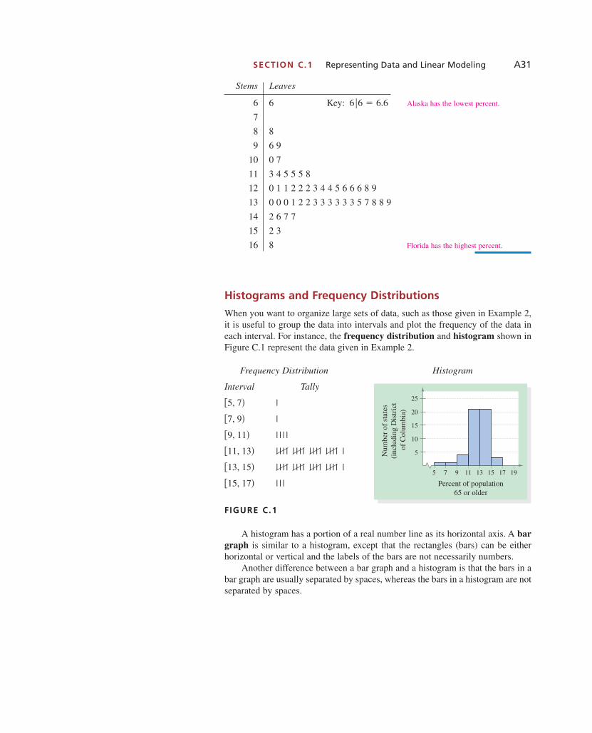
When you want to organize large sets of data, such as those given in Example 2,it is useful to group the data into intervals and plot the frequency of the data ineach interval. For instance, the frequency distribution and histogram shown inFigure C.1 represent the data given in Example 2.
Frequency Distribution Histogram
Interval Tally
FIGURE C.1
A histogram has a portion of a real number line as its horizontal axis. A bargraph is similar to a histogram, except that the rectangles (bars) can be eitherhorizontal or vertical and the labels of the bars are not necessarily numbers.
Another difference between a bar graph and a histogram is that the bars in abar graph are usually separated by spaces, whereas the bars in a histogram are notseparated by spaces.
| | |�15, 17�
|| | | || | | || | | || | | |�13, 15�
|| | | || | | || | | || | | |�11, 13�
| | | |�9, 11�
|�7, 9�
|�5, 7�
6�6 � 6.6
SECTION C.1 Representing Data and Linear Modeling A31
5 7 9 11 13 15 17 19
25
20
15
10
5
Percent of population65 or older
Num
ber
of s
tate
s (i
nclu
ding
Dis
tric
t of
Col
umbi
a)
1053715_App_C_1.qxp 11/5/08 1:21 PM Page A31
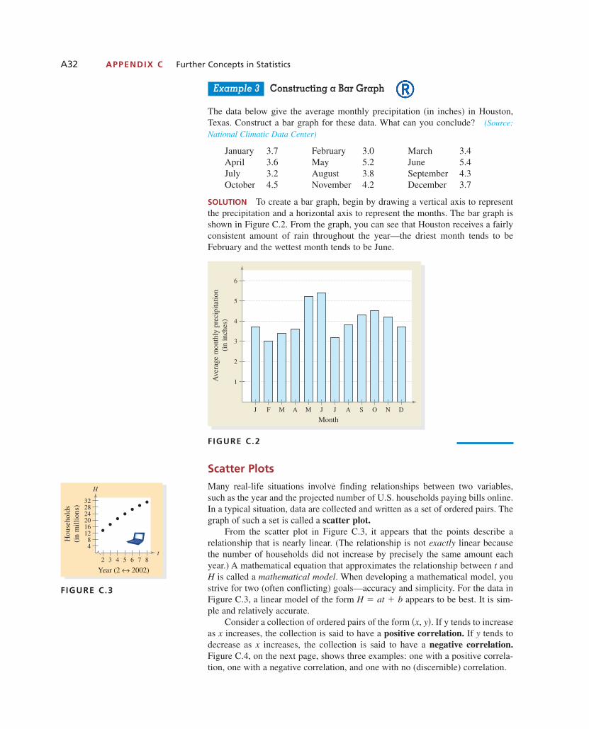
Example 3 Constructing a Bar Graph
The data below give the average monthly precipitation (in inches) in Houston,Texas. Construct a bar graph for these data. What can you conclude? (Source:National Climatic Data Center)
January 3.7 February 3.0 March 3.4April 3.6 May 5.2 June 5.4July 3.2 August 3.8 September 4.3October 4.5 November 4.2 December 3.7
SOLUTION To create a bar graph, begin by drawing a vertical axis to representthe precipitation and a horizontal axis to represent the months. The bar graph isshown in Figure C.2. From the graph, you can see that Houston receives a fairlyconsistent amount of rain throughout the year—the driest month tends to beFebruary and the wettest month tends to be June.
FIGURE C.2
Scatter Plots
Many real-life situations involve finding relationships between two variables,such as the year and the projected number of U.S. households paying bills online.In a typical situation, data are collected and written as a set of ordered pairs. Thegraph of such a set is called a scatter plot.
From the scatter plot in Figure C.3, it appears that the points describe arelationship that is nearly linear. (The relationship is not exactly linear becausethe number of households did not increase by precisely the same amount eachyear.) A mathematical equation that approximates the relationship between andH is called a mathematical model. When developing a mathematical model, youstrive for two (often conflicting) goals—accuracy and simplicity. For the data inFigure C.3, a linear model of the form appears to be best. It is sim-ple and relatively accurate.
Consider a collection of ordered pairs of the form If y tends to increaseas x increases, the collection is said to have a positive correlation. If tends todecrease as x increases, the collection is said to have a negative correlation.Figure C.4, on the next page, shows three examples: one with a positive correla-tion, one with a negative correlation, and one with no (discernible) correlation.
y�x, y�.
H � at � b
t
J F M A M J J A S O N D
1
2
3
4
5
6
Month
Ave
rage
mon
thly
pre
cipi
tatio
n(i
n in
ches
)
A32 APPENDIX C Further Concepts in Statistics
2 3 4 5 6 7 8
48
121620242832
Year (2 ↔ 2002)
Hou
seho
lds
(in
mill
ions
)
t
H
FIGURE C.3
1053715_App_C_1.qxp 11/5/08 1:21 PM Page A32

Positive Correlation Negative Correlation No Correlation
FIGURE C.4
Fitting a Line to Data
Finding a linear model that represents the relationship described by a scatter plotis called fitting a line to data. You can do this graphically by simply sketchingthe line that appears to fit the points, finding two points on the line, and then find-ing the equation of the line that passes through the two points.
Example 4 Fitting a Line to Data
Find a linear model that relates the year with the projected number of U.S. house-holds H (in millions) that will pay bills online for the years 2002 through 2008.(Source: Forrester Research)
SOLUTION Let t represent the year, with corresponding to 2002. Afterplotting the data from the table, draw the line that you think best represents thedata, as shown in Figure C.5. Two points that lie on this line are and
Using the point-slope form, you can find the equation of the line to be
Linear model
FIGURE C.5
2 3 4 5 6 7 8
4
8
12
16
20
24
28
32
Year (2 ↔ 2002)
Hou
seho
lds
(in
mill
ions
)
t
H
H = 3t � 8.9
H � 3�t � 4� � 20.9 � 3t � 8.9.
�5, 23.9�.�4, 20.9�
t � 2
xx x
y y y
SECTION C.1 Representing Data and Linear Modeling A33
S T U D Y T I PThe model in Example 4 isbased on the two data pointschosen. If different points arechosen, the model may changesomewhat. For instance, if you choose and
the new model isH � 2.25t � 13.2.�8, 31.2�,
�6, 26.7�
Year 2002 2003 2004 2005 2006 2007 2008
Households, H 13.7 17.4 20.9 23.9 26.7 29.1 31.2
1053715_App_C_1.qxp 11/5/08 1:21 PM Page A33
Once you have found a model, you can measure how well the model fits thedata by comparing the actual values with the values given by the model, as shownin the following table.
The sum of the squares of the differences between the actual values and themodel values is the sum of the squared differences. The model that has the leastsum is called the least squares regression line for the data. For the model inExample 4, the sum of the squared differences is 5.26. The least squares regres-sion line for the data is
Best-fitting linear model
Its sum of squared differences is approximately 2.31.
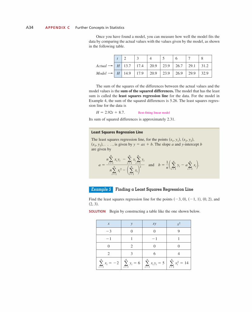
Example 5 Finding a Least Squares Regression Line
Find the least squares regression line for the points and
SOLUTION Begin by constructing a table like the one shown below.
�2, 3�.�0, 2�,��1, 1�,��3, 0�,
H � 2.92t � 8.7.
A34 APPENDIX C Further Concepts in Statistics
t 2 3 4 5 6 7 8
H 13.7 17.4 20.9 23.9 26.7 29.1 31.2
H 14.9 17.9 20.9 23.9 26.9 29.9 32.9
x y xy x2
�3 0 0 9
�1 1 �1 1
0 2 0 0
2 3 6 4
�n
i�1 xi � �2 �
n
i�1 yi � 6 �
n
i�1 xi yi � 5 �
n
i�1 x2
i � 14
Actual
Model
Least Squares Regression Line
The least squares regression line, for the points is given by The slope and intercept
are given by
and b �1n � �
n
i�1 yi � a�
n
i�1 xi�.a �
n�n
i�1 xi yi � �
n
i�1 xi �
n
i�1 yi
n�n
i�1 x 2
i � ��n
i�1 xi�2
by-ay � ax � b.�x3, y3�, . . . ,�x2, y2�,�x1, y1�,
1053715_App_C_1.qxp 11/5/08 1:21 PM Page A34
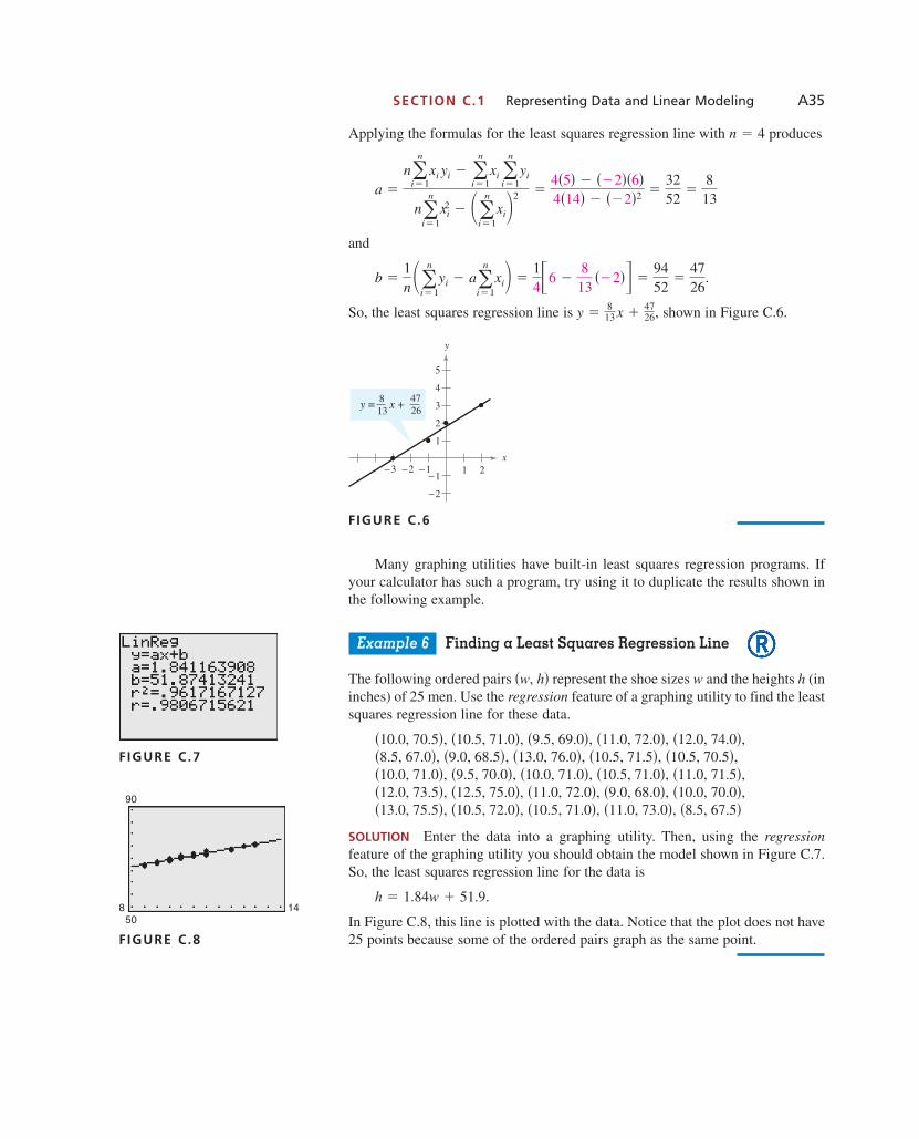
Applying the formulas for the least squares regression line with produces
and
So, the least squares regression line is shown in Figure C.6.
FIGURE C.6
Many graphing utilities have built-in least squares regression programs. Ifyour calculator has such a program, try using it to duplicate the results shown inthe following example.
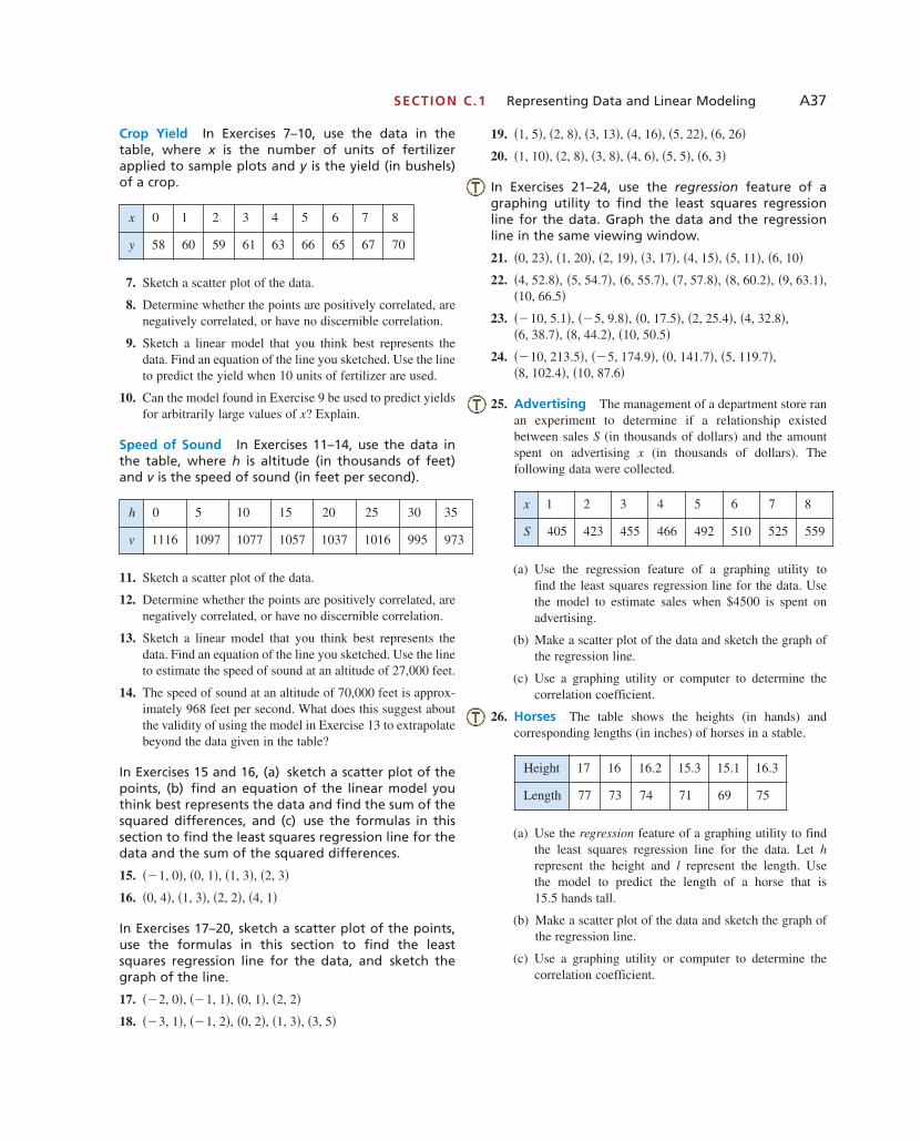
Example 6 Finding a Least Squares Regression Line
The following ordered pairs represent the shoe sizes w and the heights h (ininches) of 25 men. Use the regression feature of a graphing utility to find the leastsquares regression line for these data.
,
SOLUTION Enter the data into a graphing utility. Then, using the regressionfeature of the graphing utility you should obtain the model shown in Figure C.7.So, the least squares regression line for the data is
In Figure C.8, this line is plotted with the data. Notice that the plot does not have25 points because some of the ordered pairs graph as the same point.
h � 1.84w � 51.9.
�8.5, 67.5��11.0, 73.0�,�10.5, 71.0�,�10.5, 72.0�,�13.0, 75.5�,�10.0, 70.0�,�9.0, 68.0�,�11.0, 72.0�,�12.5, 75.0�,�12.0, 73.5�,�11.0, 71.5�,�10.5, 71.0�,�10.0, 71.0�,�9.5, 70.0�,�10.0, 71.0�,
�10.5, 70.5�,�10.5, 71.5�,�13.0, 76.0�,�9.0, 68.5��8.5, 67.0�,�12.0, 74.0�,�11.0, 72.0�,�9.5, 69.0�,�10.5, 71.0�,�10.0, 70.5�,
�w, h�
y
x
y = x + 813
4726
−1−2−3 1 2−1
−2
1
2
3
4
5
y �813 x �
4726,
b �1n ��
n
i�1yi � a�
n
i�1xi� �
146 �
813
��2� �9452
�4726
.
a �
n�n
i�1xi yi � �
n
i�1xi �
n
i�1yi
n�n
i�1xi2 � ��
n
i�1xi�
2 �4�5� � ��2��6�4�14� � ��2�2 �
3252
�813
n � 4
SECTION C.1 Representing Data and Linear Modeling A35
FIGURE C.7
8 1450
90
FIGURE C.8
1053715_App_C_1.qxp 11/5/08 1:21 PM Page A35

If you use the regression feature of a graphing utility or a computer programto duplicate the results of Example 6, you will notice that the program may alsooutput an value. For instance, the value from Example 6 was Thisnumber is called the correlation coefficient of the data and gives a measure ofhow well the model fits the data. Correlation coefficients vary between and1. Basically, the closer is to 1, the better the points can be described by a line.Three examples are shown in Figure C.9.
FIGURE C.9
900
900
900
1818 18
r = 0.981 r = 0.190r = −0.866
�r��1
r � 0.981.r-r-
A36 APPENDIX C Further Concepts in Statistics
Exam Scores In Exercises 1 and 2, use the followingscores from a math class with 30 students. The scoresare given for two 100-point exams.
Exam #1: 77, 100, 77, 70, 83, 89, 87, 85, 81, 84, 81, 78,89, 78, 88, 85, 90, 92, 75, 81, 85, 100, 98, 81, 78, 75, 85,89, 82, 75
Exam #2: 76, 78, 73, 59, 70, 81, 71, 66, 66, 73, 68, 67,63, 67, 77, 84, 87, 71, 78, 78, 90, 80, 77, 70, 80, 64, 74,68, 68, 68
1. Construct a stem-and-leaf plot for Exam #1.
2. Construct a double stem-and-leaf plot to compare the scoresfor Exam #1 and Exam #2. Which set of test scores is better?
3. Cancer The table shows the estimated numbers of newcancer cases (in thousands) in the 50 states in 2006. Use astem-and-leaf plot to organize the data. (Source: AmericanCancer Society, Inc.)
4. Snowfall The data give the seasonal snowfalls (in inches) for Lincoln, Nebraska for the years 1970 through2006 (the amounts are listed in order by year). How wouldyou organize these data? Explain your reasoning. (Source:National Weather Service)
49.0, 21.6, 29.2, 33.6, 42.1, 21.1, 21.8, 31.0, 34.4, 23.3,13.0, 32.3, 38.0, 47.5, 21.5, 18.9, 15.7, 13.0, 19.1, 18.7,25.8, 23.8, 32.1, 21.3, 21.7, 30.7, 29.0, 44.6, 24.4, 11.7,37.9, 29.5, 31.7, 35.9, 16.3, 19.5
5. Bus Fares The data below give the base prices of bus farein selected U.S. cities. Construct a bar graph for these data.(Source: American Public Transportation Association)
Seattle $1.25 Atlanta $1.75
Houston $1.00 Dallas $1.25
New York $2.00 Denver $1.15
Los Angeles $1.35 Chicago $1.50
6. Melanoma The data below give the places of origin andthe estimated numbers of new melanoma cases in 2006.Construct a bar graph for these data. (Source: AmericanCancer Society, Inc.)
California 6290 Florida 4870
Michigan 1890 New York 3380
Texas 3930 Washington 1490
Exercises C.1
AL 24 AK 2 AZ 26 AR 15 CA 139CO 17 CT 17 DE 4 FL 99 GA 37HI 6 ID 6 IL 60 IN 33 IA 16KS 13 KY 24 LA 24 ME 8 MD 26MA 33 MI 48 MN 24 MS 15 MO 31MT 5 NE 9 NV 12 NH 7 NJ 44NM 8 NY 88 NC 41 ND 3 OH 61OK 19 OR 18 PA 74 RI 6 SC 23SD 4 TN 32 TX 86 UT 7 VT 3VA 35 WA 28 WV 11 WI 26 WY 3
1053715_App_C_1.qxp 11/5/08 1:21 PM Page A36
SECTION C.1 Representing Data and Linear Modeling A37
Crop Yield In Exercises 7–10, use the data in thetable, where x is the number of units of fertilizerapplied to sample plots and y is the yield (in bushels)of a crop.
7. Sketch a scatter plot of the data.
8. Determine whether the points are positively correlated, arenegatively correlated, or have no discernible correlation.
9. Sketch a linear model that you think best represents thedata. Find an equation of the line you sketched. Use the lineto predict the yield when 10 units of fertilizer are used.
10. Can the model found in Exercise 9 be used to predict yieldsfor arbitrarily large values of x? Explain.
Speed of Sound In Exercises 11–14, use the data inthe table, where h is altitude (in thousands of feet)and v is the speed of sound (in feet per second).
11. Sketch a scatter plot of the data.
12. Determine whether the points are positively correlated, arenegatively correlated, or have no discernible correlation.
13. Sketch a linear model that you think best represents thedata. Find an equation of the line you sketched. Use the lineto estimate the speed of sound at an altitude of 27,000 feet.
14. The speed of sound at an altitude of 70,000 feet is approx-imately 968 feet per second. What does this suggest aboutthe validity of using the model in Exercise 13 to extrapolatebeyond the data given in the table?
In Exercises 15 and 16, (a) sketch a scatter plot of thepoints, (b) find an equation of the linear model youthink best represents the data and find the sum of thesquared differences, and (c) use the formulas in thissection to find the least squares regression line for thedata and the sum of the squared differences.
15.
16.
In Exercises 17–20, sketch a scatter plot of the points,use the formulas in this section to find the leastsquares regression line for the data, and sketch thegraph of the line.
17.
18.
19.
20.
In Exercises 21–24, use the regression feature of agraphing utility to find the least squares regressionline for the data. Graph the data and the regressionline in the same viewing window.
21.
22.
23.
24.
25. Advertising The management of a department store ranan experiment to determine if a relationship existedbetween sales S (in thousands of dollars) and the amountspent on advertising x (in thousands of dollars). The following data were collected.
(a) Use the regression feature of a graphing utility to find the least squares regression line for the data. Usethe model to estimate sales when $4500 is spent on advertising.
(b) Make a scatter plot of the data and sketch the graph ofthe regression line.
(c) Use a graphing utility or computer to determine thecorrelation coefficient.
26. Horses The table shows the heights (in hands) and corresponding lengths (in inches) of horses in a stable.
(a) Use the regression feature of a graphing utility to findthe least squares regression line for the data. Let hrepresent the height and l represent the length. Use the model to predict the length of a horse that is 15.5 hands tall.
(b) Make a scatter plot of the data and sketch the graph ofthe regression line.
(c) Use a graphing utility or computer to determine thecorrelation coefficient.
�10, 87.6��8, 102.4�,�5, 119.7�,�0, 141.7�,��5, 174.9�,��10, 213.5�,
�10, 50.5��8, 44.2�,�6, 38.7�,�4, 32.8�,�2, 25.4�,�0, 17.5�,��5, 9.8�,��10, 5.1�,
�10, 66.5��9, 63.1�,�8, 60.2�,�7, 57.8�,�6, 55.7�,�5, 54.7�,�4, 52.8�,
�6, 10��5, 11�,�4, 15�,�3, 17�,�2, 19�,�1, 20�,�0, 23�,
�1, 10�, �2, 8�, �3, 8�, �4, 6�, �5, 5�, �6, 3��1, 5�, �2, 8�, �3, 13�, �4, 16�, �5, 22�, �6, 26�
��3, 1�, ��1, 2�, �0, 2�, �1, 3�, �3, 5���2, 0�, ��1, 1�, �0, 1�, �2, 2�
�0, 4�, �1, 3�, �2, 2�, �4, 1���1, 0�, �0, 1�, �1, 3�, �2, 3�
x 0 1 2 3 4 5 6 7 8
y 58 60 59 61 63 66 65 67 70
x 1 2 3 4 5 6 7 8
S 405 423 455 466 492 510 525 559
h 0 5 10 15 20 25 30 35
v 1116 1097 1077 1057 1037 1016 995 973
Height 17 16 16.2 15.3 15.1 16.3
Length 77 73 74 71 69 75
1053715_App_C_1.qxp 11/5/08 1:21 PM Page A37
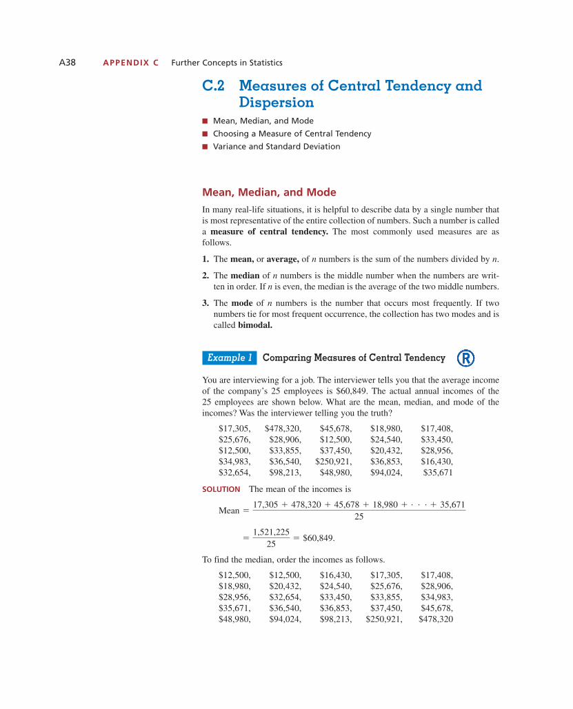
A38 APPENDIX C Further Concepts in Statistics
Mean, Median, and Mode
In many real-life situations, it is helpful to describe data by a single number thatis most representative of the entire collection of numbers. Such a number is calleda measure of central tendency. The most commonly used measures are as follows.
1. The mean, or average, of n numbers is the sum of the numbers divided by n.
2. The median of n numbers is the middle number when the numbers are writ-ten in order. If n is even, the median is the average of the two middle numbers.
3. The mode of n numbers is the number that occurs most frequently. If twonumbers tie for most frequent occurrence, the collection has two modes and iscalled bimodal.
Example 1 Comparing Measures of Central Tendency
You are interviewing for a job. The interviewer tells you that the average incomeof the company’s 25 employees is $60,849. The actual annual incomes of the 25 employees are shown below. What are the mean, median, and mode of theincomes? Was the interviewer telling you the truth?
$17,305, $478,320, $45,678, $18,980, $17,408,$25,676, $28,906, $12,500, $24,540, $33,450,$12,500, $33,855, $37,450, $20,432, $28,956,$34,983, $36,540, $250,921, $36,853, $16,430,$32,654, $98,213, $48,980, $94,024, $35,671
SOLUTION The mean of the incomes is
To find the median, order the incomes as follows.
$12,500, $12,500, $16,430, $17,305, $17,408,$18,980, $20,432, $24,540, $25,676, $28,906,$28,956, $32,654, $33,450, $33,855, $34,983,$35,671, $36,540, $36,853, $37,450, $45,678,$48,980, $94,024, $98,213, $250,921, $478,320
�1,521,225
25� $60,849.
Mean �17,305 � 478,320 � 45,678 � 18,980 � . . . � 35,671
25
C.2 Measures of Central Tendency andDispersion
■ Mean, Median, and Mode
■ Choosing a Measure of Central Tendency
■ Variance and Standard Deviation
1053715_App_C_2.qxp 11/5/08 1:21 PM Page A38

SECTION C.2 Measures of Central Tendency and Dispersion A39
From this list, you can see the median income is $33,450. You can also see that$12,500 is the only income that occurs more than once. So, the mode is $12,500.Technically, the interviewer was telling the truth because the average is (general-ly) defined to be the mean. However, of the three measures of central tendency
Mean: $60,849 Median: $33,450 Mode: $12,500
it seems clear that the median is most representative. The mean is inflated by thetwo highest salaries.
Choosing a Measure of Central Tendency
Which of the three measures of central tendency is the most representative? Theanswer is that it depends on the distribution of the data and the way in which youplan to use the data.
For instance, in Example 1, the mean salary of $60,849 does not seem veryrepresentative to a potential employee. To a city income tax collector who wantsto estimate 1% of the total income of the 25 employees, however, the mean isprecisely the right measure.
Example 2 Choosing a Measure of Central Tendency
Which measure of central tendency is the most representative of the data shownin each frequency distribution?
a.
b.
c.
SOLUTION
a. For these data, the mean is about 4.23, the median is 3, and the mode is 2. Of these, the mode is probably the most representative measure.
b. For these data, the mean and median are each 5 and the modes are 1 and 9(the distribution is bimodal). Of these, the mean or median is the mostrepresentative measure.
c. For these data, the mean is most 4.59, the median is 5, and the mode is 1. Of these, the mean or median is the most representative measure.
Number 1 2 3 4 5 6 7 8 9
Frequency 6 1 2 3 5 5 4 3 0
Number 1 2 3 4 5 6 7 8 9
Frequency 9 8 7 6 5 6 7 8 9
Number 1 2 3 4 5 6 7 8 9
Frequency 7 20 15 11 8 3 2 0 15
1053715_App_C_2.qxp 11/5/08 1:21 PM Page A39
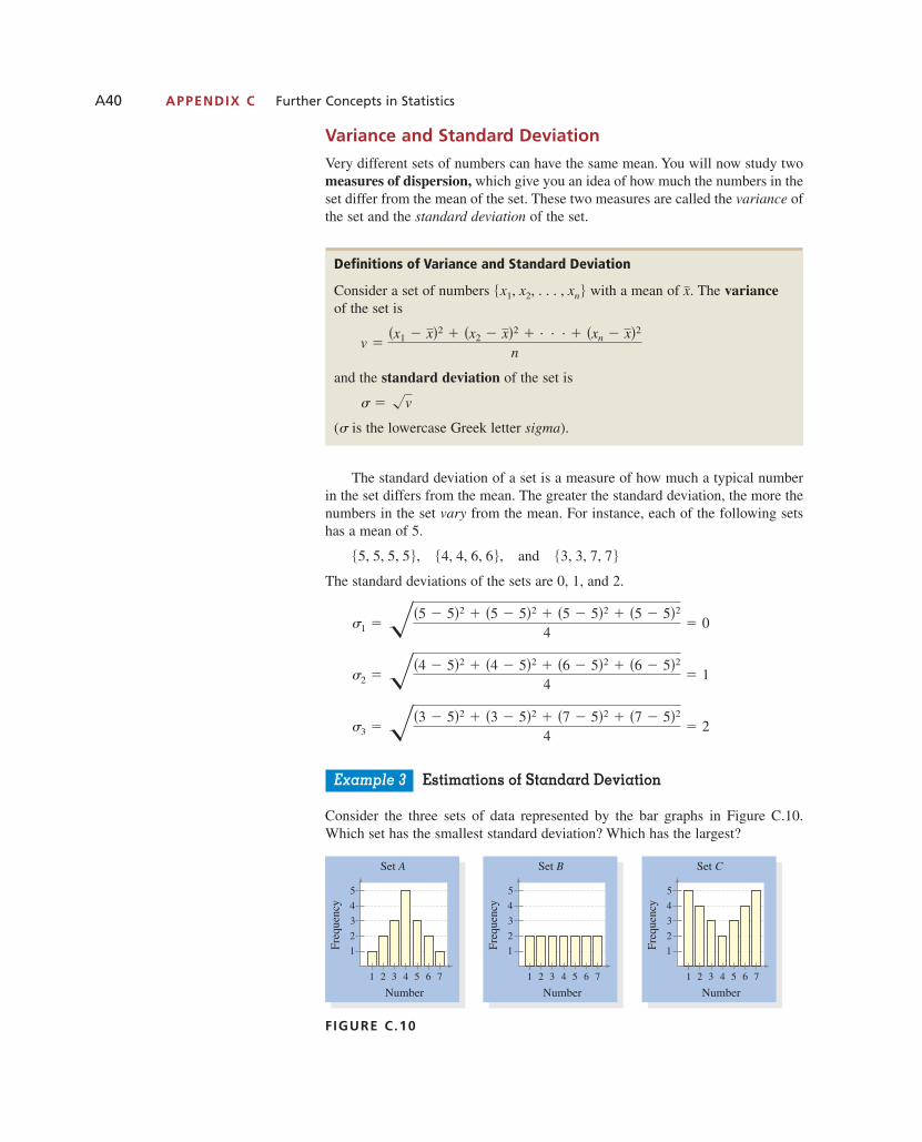
A40 APPENDIX C Further Concepts in Statistics
Variance and Standard Deviation
Very different sets of numbers can have the same mean. You will now study twomeasures of dispersion, which give you an idea of how much the numbers in theset differ from the mean of the set. These two measures are called the variance ofthe set and the standard deviation of the set.
The standard deviation of a set is a measure of how much a typical numberin the set differs from the mean. The greater the standard deviation, the more thenumbers in the set vary from the mean. For instance, each of the following setshas a mean of 5.
and
The standard deviations of the sets are 0, 1, and 2.
Example 3 Estimations of Standard Deviation
Consider the three sets of data represented by the bar graphs in Figure C.10.Which set has the smallest standard deviation? Which has the largest?
FIGURE C.10
4
5
3
2
1Freq
uenc
y
Number
1 2 3 4 5 6 7
Set A
4
5
3
2
1Freq
uenc
y
Number
1 2 3 4 5 6 7
Set B
4
5
3
2
1Freq
uenc
y
Number
1 2 3 4 5 6 7
Set C
�3 ���3 � 5�2 � �3 � 5�2 � �7 � 5�2 � �7 � 5�2
4 � 2
�2 ���4 � 5�2 � �4 � 5�2 � �6 � 5�2 � �6 � 5�2
4 � 1
�1 ���5 � 5�2 � �5 � 5�2 � �5 � 5�2 � �5 � 5�2
4 � 0
�3, 3, 7, 7��4, 4, 6, 6�,�5, 5, 5, 5�,
Definitions of Variance and Standard Deviation
Consider a set of numbers with a mean of The varianceof the set is
and the standard deviation of the set is
( is the lowercase Greek letter sigma).�
� � �v
v ��x1 � x�2 � �x2 � x�2 � . . . � �xn � x�2
n
x.�x1, x2, . . . , xn�
1053715_App_C_2.qxp 11/5/08 1:21 PM Page A40

SOLUTION Of the three sets, the numbers in set A are grouped most closely tothe center and the numbers in set C are the most dispersed. So, set A has thesmallest standard deviation and set C has the largest standard deviation.
Example 4 Finding Standard Deviation
Find the standard deviation of each set shown in Example 3.
SOLUTION Because of the symmetry of each bar graph, you can conclude thateach has a mean of The standard deviation of set A is
The standard deviation of set B is
The standard deviation of set C is
These values confirm the results of Example 3. That is, set A has the smalleststandard deviation and set C has the largest.
The following alternative formula provides a more efficient way to computethe standard deviation.
Because of lengthy computations, this formula is difficult to verify. Con-ceptually, however, the process is straightforward. It consists of showing that the expressions
and
are equivalent. Try verifying this equivalence for the set withx � �x1 � x2 � x3��3.
�x1, x2, x3�
�x12 � x2
2 � . . . � xn2
n� x2
��x1 � x�2 � �x2 � x�2 � . . . � �xn � x�2
n
� 2.22.
� ��5��3�2 � 4��2�2 � 3��1�2 � 2�0�2 � 3�1�2 � 4�2�2 � 5�3�2
26
� 2.
� ��2��3�2 � 2��2�2 � 2��1�2 � 2�0�2 � 2�1�2 � 2�2�2 � 2�3�2
14
� 1.53.
� ��(�3�2 � 2��2�2 � 3��1�2 � 5�0�2 � 3�1�2 � 2�2�2 � �3�2
17
x � 4.
SECTION C.2 Measures of Central Tendency and Dispersion A41
Alternative Formula for Standard Deviation
The standard deviation of is
� ��x12 � x2
2 � . . . � xn2
n� x2.
�x1, x2, . . . , xn�
1053715_App_C_2.qxp 11/5/08 1:21 PM Page A41

Example 5 Using the Alternative Formula
Use the alternative formula for standard deviation to find the standard deviationof the following set of numbers.
5, 6, 6, 7, 7, 8, 8, 8, 9, 10
SOLUTION Begin by finding the mean of the set, which is 7.4. So, the standarddeviation is
You can use the statistical features of a graphing utility to check this result.
A well-known theorem in statistics, called Chebychev’s Theorem, states thatat least
of the numbers in a distribution must lie within k standard deviations of the mean.So, 75% of the numbers in a collection must lie within two standard deviations of the mean, and at least 88.9% of the numbers must lie within three standarddeviations of the mean. For most distributions, these percentages are low. Forinstance, in all three distributions shown in Example 3, 100% of the numbers liewithin two standard deviations of the mean.
Example 6 Describing a Distribution
The table shows the numbers of nurses (per 100,000 people) in each state and theDistrict of Columbia. Find the mean and standard deviation of the data. Whatpercent of the numbers lie within two standard deviations of the mean? (Source:U.S. Department of Health and Human Services)
1 �1k2
� 1.43.
� �2.04
��56810
� 54.76
� ��52 � 2�62� � 2�72� � 3�82� � 92 � 102
10� �7.4�2
A42 APPENDIX C Further Concepts in Statistics
AL 796 AK 801 AZ 671 AR 727 CA 545CO 773 CT 982 DE 921 DC 1520 FL 805GA 709 HI 707 ID 642 IL 842 IN 815IA 1020 KS 908 KY 842 LA 798 ME 1039MD 814 MA 1191 MI 837 MN 943 MS 761MO 938 MT 841 NE 920 NV 533 NH 878NJ 878 NM 627 NY 866 NC 877 ND 995OH 908 OK 652 OR 751 PA 1089 RI 1062SC 688 SD 1100 TN 848 TX 609 UT 601VT 951 VA 776 WA 763 WV 860 WI 915WY 759
1053715_App_C_2.qxp 11/5/08 1:21 PM Page A42

SOLUTION Begin by entering the numbers into a graphing utility that has a standard deviation program. After running the program, you should obtain
and
The interval that contains all numbers that lie within two standard deviations ofthe mean is
or
From the table, you can see that all but two of the numbers (96%) lie in thisinterval—all but the numbers that correspond to the number of nurses (per100,000 people) in Washington, DC and Massachusetts.
501.7, 1187.3.844.5 � 2�171.4�, 844.5 � 2�171.4�
� � 171.4.x � 844.5
SECTION C.2 Measures of Central Tendency and Dispersion A43
In Exercises 1–6, find the mean, median, and mode ofthe set of measurements.
1. 5, 12, 7, 14, 8, 9, 7
2. 30, 37, 32, 39, 33, 34, 32
3. 5, 12, 7, 24, 8, 9, 7
4. 20, 37, 32, 39, 33, 34, 32
5. 5, 12, 7, 14, 9, 7
6. 30, 37, 32, 39, 34, 32
7. Reasoning Compare your answers for Exercises 1 and 3with those for Exercises 2 and 4. Which of the measures ofcentral tendency is sensitive to extreme measurements?Explain your reasoning.
8. Reasoning
(a) Add 6 to each measurement in Exercise 1 and calculatethe mean, median, and mode of the revised measure-ments. How are the measures of central tendencychanged?
(b) If a constant k is added to each measurement in a set of data, how will the measures of central tendencychange?
9. Electric Bills A person had the following monthly bills forelectricity. What are the mean and median of the collectionof bills?
January $67.92 February $59.84
March $52.00 April $52.50
May $57.99 June $65.35
July $81.76 August $74.98
September $87.82 October $83.18
November $65.35 December $57.00
10. Car Rental A car rental company kept the followingrecord of the numbers of miles a rental car was driven.What are the mean, median, and mode of these data?
Monday 410 Tuesday 260
Wednesday 320 Thursday 320
Friday 460 Saturday 150
11. Six-Child Families A study was done on families havingsix children. The table shows the numbers of families in thestudy with the indicated number of girls. Determine themean, median, and mode of this set of data.
12. Baseball A baseball fan examined the records of afavorite baseball player’s performance during his last 50games. The numbers of games in which the player had 0, 1,2, 3, and 4 hits are recorded in the table.
(a) Determine the average number of hits per game.
(b) Determine the player’s batting average if he had 200 atbats during the 50-game series.
13. Think About It Construct a collection of numbers thathas the following properties. If this is not possible, explainwhy it is not.
Mean � 6, median � 4, mode � 4
Exercises C.2
Number of girls 0 1 2 3 4 5 6
Frequency 1 24 45 54 50 19 7
Number of hits 0 1 2 3 4
Frequency 14 26 7 2 1
1053715_App_C_2.qxp 11/5/08 1:21 PM Page A43

14. Think About It Construct a collection of numbers thathas the following properties. If this is not possible, explainwhy it is not.
15. Test Scores A philosophy professor records the follow-ing scores for a 100-point exam.
99, 64, 80, 77, 59, 72, 87, 79, 92, 88, 90, 42, 20, 89, 42,100, 98, 84, 78, 91
Which measure of central tendency best describes thesetest scores?
16. Shoe Sales A salesman sold eight pairs of men’s dressshoes. The sizes of the eight pairs were as follows: 8,12, 10, 11 and Which measure (or measures)of central tendency best describes the typical shoe size forthese data?
In Exercises 17–24, find the mean ( ), variance (v), andstandard deviation ( ) of the data set.
17. 4, 10, 8, 2
18. 3, 15, 6, 9, 2
19. 0, 1, 1, 2, 2, 2, 3, 3, 4
20. 2, 2, 2, 2, 2, 2
21. 1, 2, 3, 4, 5, 6, 7
22. 1, 1, 1, 5, 5, 5
23. 49, 62, 40, 29, 32, 70
24. 1.5, 0.4, 2.1, 0.7, 0.8
In Exercises 25–30, use the alternative formula to findthe standard deviation of the data set.
25. 2, 4, 6, 6, 13, 5
26. 10, 25, 50, 26, 15, 33, 29, 4
27. 246, 336, 473, 167, 219, 359
28. 6.0, 9.1, 4.4, 8.7, 10.4
29. 8.1, 6.9, 3.7, 4.2, 6.1
30. 9.0, 7.5, 3.3, 7.4, 6.0
31. Reasoning Without calculating the standard deviation,explain why the set has a standard deviationof 8.
32. Reasoning If the standard deviation of a set of numbersis 0, what does this imply about the set?
33. Test Scores An instructor adds five points to each student’s exam score. Will this change the mean or standarddeviation of the exam scores? Explain.
34. Think About It Consider the four sets of data representedby the histograms. Order the sets from the smallest to thelargest variance.
35. Test Scores The scores of a mathematics exam given to600 science and engineering students at a college had amean and standard deviation of 235 and 28, respectively.Use Chebychev’s Theorem to determine the intervals con-
taining at least and at least of the scores. How would theintervals change if the standard deviation were 16?
36. Price of Gold The data represent the average prices ofgold (in dollars per ounce) for the years 1987 to 2006. Usea graphing utility or computer to find the mean, variance,and standard deviation of the data. What percent of the datalie within two standard deviations of the mean? (Source:Kitco.com)
446, 437, 381, 384, 362,344, 360, 384, 384, 388,331, 294, 279, 279, 271,310, 363, 410, 445, 603
37. Price of Silver The data represent the average prices ofsilver (in dollars per ounce) for the years 1987 to 2006. Usea graphing utility or computer to find the mean, variance,and standard deviation of the data. What percent of the datalie within one standard deviation of the mean? (Source:Kitco.com)
6.79, 6.11, 5.54, 4.07, 3.91,3.71, 4.97, 4.77, 5.15, 4.73,5.95, 5.55, 5.22, 4.95, 4.37,4.60, 4.88, 6.67, 7.32, 11.55
89
34
1 2 3 4
2
4
6
8
Number
Freq
uenc
y
Set D
1 2 3 4
2
4
6
8
NumberFr
eque
ncy
Set C
1 2 3 4
2
4
6
8
Number
Freq
uenc
y
Set B
1 2 3 4
2
4
6
8
Number
Freq
uenc
y
Set A
�4, 4, 20, 20�
�x
1012.91
2,1012,
1012,
Mean � 6, median � 6, mode � 4
A44 APPENDIX C Further Concepts in Statistics
1053715_App_C_2.qxp 11/5/08 1:21 PM Page A44

APPENDIX D Alternative Introduction to the Fundamental Theorem of Calculus A45
■ Approximate the areas of regions using Riemann sums.
■ Evaluate definite integrals.
In this appendix, a summation process is used to provide an alternativedevelopment of the definite integral. It is intended that this supplement followSection 11.3 in the text. If used, this appendix should replace the materialpreceding Example 2 in Section 11.4. Example 1 below shows how the area of aregion in the plane can be approximated by the use of rectangles.
Example 1 Using Rectangles to Approximate the Area of a Region
Use the four rectangles indicated in Figure D.1 to approximate the area of theregion lying between the graph of
and the x-axis, between and
SOLUTION You can find the heights of the rectangles by evaluating the functionf at each of the midpoints of the subintervals
Because the width of each rectangle is 1, the sum of the areas of the fourrectangles is
So, you can approximate the area of the region to be 10.5 square units.
� 10.5.
�848
�18
�98
�258
�498
S � �1� f �12� � �1� f �3
2� � �1� f �52� � �1� f �7
2�
�0, 1�, �1, 2�, �2, 3�, �3, 4�.
x � 4.x � 0
f�x� �x2
2
S T U D Y T I PThe approximation technique used in Example 1 is called the MidpointRule. The Midpoint Rule is discussed further in Section 11.6.
8
6
4
2
x
y
1 2 3 4
f (x) = x2
2
FIGURE D.1
widthheight
width width widthheight height height
D Alternative Introduction to theFundamental Theorem of Calculus
1053715_App_D.qxp 11/5/08 1:22 PM Page A45

A46 APPENDIX D Alternative Introduction to the Fundamental Theorem of Calculus
The procedure shown in Example 1 can be generalized. Let f be a continuousfunction defined on the closed interval To begin, partition the interval inton subintervals, each of width as shown.
In each subinterval choose an arbitrary point and form the sum
This type of summation is called a Riemann sum, and is often written using sum-mation notation as shown below.
For the Riemann sum in Example 1, the interval is the number of subintervals is the width of each subinterval is and the point in each subinterval is its midpoint. So, you can write the approximation inExample 1 as
Example 2 Using a Riemann Sum to Approximate Area
Use a Riemann sum to approximate the area of the region bounded by the graphof and the x-axis, for In the Riemann sum, let
and choose to be the left endpoint of each subinterval.
SOLUTION Subdivide the interval into six subintervals, each of width
as shown in Figure D.2. Because is the left endpoint of each subinterval, theRiemann sum is given by
�3527
square units .
� �0 �59
�89
� 1 �89
�59�
13�
� �f �0� � f �13� � f �2
3� � f �1� � f �43� � f �5
3��13�
S � n
i�1 f�ci� �x
ci
�13
�x �2 � 0
6
�0, 2�
cin � 60 ≤ x ≤ 2.f�x� � �x2 � 2x
�848
.
�18
�98
�258
�498
� 4
i�1 f �ci��1�
S � n
i�1 f(ci� �x
ci�x � 1,n � 4,�a, b� � �0, 4�,
xi�1 ≤ ci ≤ xiS � n
i�1 f�ci� �x,
S � f�c1� �x � f�c2� �x � . . . � f�cn�1� �x � f�cn� �x.
ci�xi�1, xi�,
a � x0 < x1 < x2 < . . . < xn�1 < xn � b
�x � �b � a��n,�a, b�.
x1
1
2
y
13
23
43
53
f (x) = −x2 + 2x
FIGURE D.2
1053715_App_D.qxp 11/5/08 1:22 PM Page A46
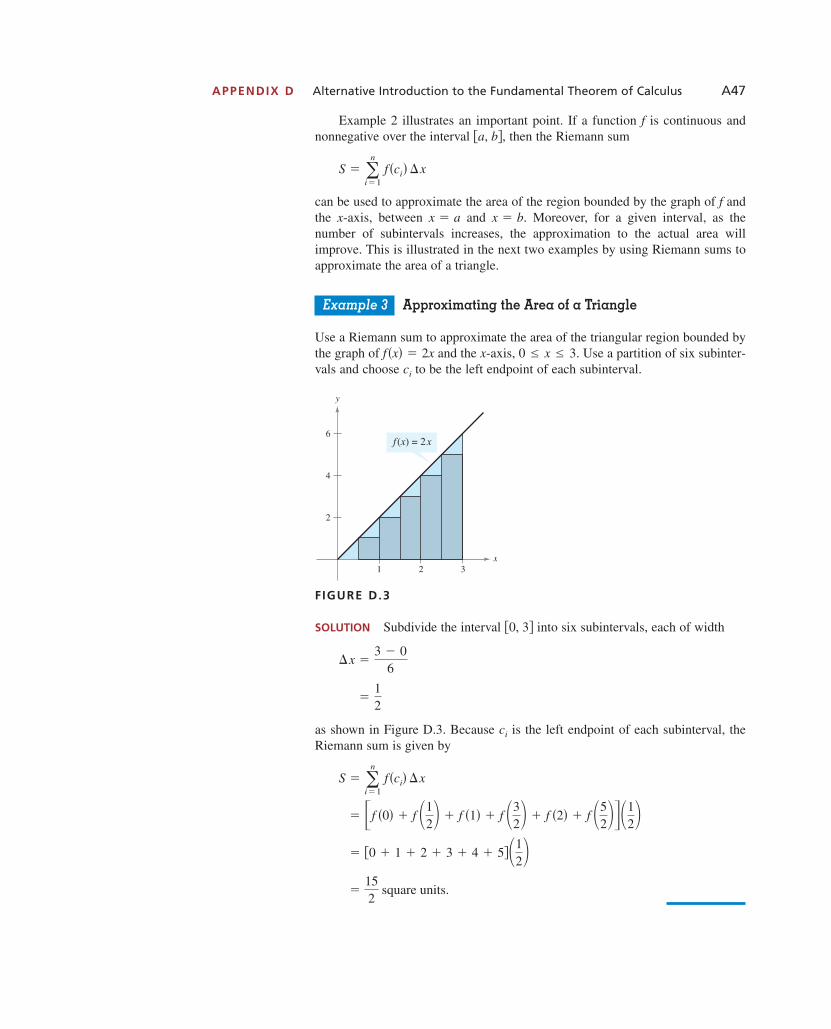
Example 2 illustrates an important point. If a function f is continuous andnonnegative over the interval then the Riemann sum
can be used to approximate the area of the region bounded by the graph of f andthe x-axis, between and Moreover, for a given interval, as the number of subintervals increases, the approximation to the actual area willimprove. This is illustrated in the next two examples by using Riemann sums toapproximate the area of a triangle.
Example 3 Approximating the Area of a Triangle
Use a Riemann sum to approximate the area of the triangular region bounded bythe graph of and the x-axis, Use a partition of six subinter-vals and choose to be the left endpoint of each subinterval.
FIGURE D.3
SOLUTION Subdivide the interval into six subintervals, each of width
as shown in Figure D.3. Because is the left endpoint of each subinterval, theRiemann sum is given by
�152
square units.
� �0 � 1 � 2 � 3 � 4 � 5��12�
� �f �0� � f �12� � f �1� � f �3
2� � f �2� � f �52��
12�
S � n
i�1 f�ci� �x
ci
�12
�x �3 � 0
6
�0, 3�
x
6
4
2
y
1 2 3
f (x) = 2x
ci
0 ≤ x ≤ 3.f�x� � 2x
x � b.x � a
S � n
i�1 f�ci� �x
�a, b�,
APPENDIX D Alternative Introduction to the Fundamental Theorem of Calculus A47
1053715_App_D.qxp 11/5/08 1:22 PM Page A47

A48 APPENDIX D Alternative Introduction to the Fundamental Theorem of Calculus
The approximations in Examples 2 and 3 are called left Riemann sums,because was chosen to be the left endpoint of each subinterval. If the right endpoints had been used in Example 3, the right Riemann sum would have been
Note that the exact area of the triangular region in Example 3 is
So, the left Riemann sum gives an approximation that is less than the actual area,and the right Riemann sum gives an approximation that is greater than the actualarea.
In Example 4, you will see that the approximation improves as the numberof subintervals increases.
Example 4 Increasing the Number of Subintervals
Let Use a computer to determine the left and rightRiemann sums for and subintervals.
SOLUTION A basic computer program for this problem is as shown.
10 INPUT; N
20 DELTA=3/N
30 LSUM=0: RSUM=0
40 FOR I=1 TO N
50 LC=(I-1)*DELTA: RC=I*DELTA
60 LSUM=LSUM+2*LC*DELTA: RSUM=RSUM+2*RC*DELTA
70 NEXT
80 PRINT “LEFT RIEMANN SUM:”; LSUM
90 PRINT “RIGHT RIEMANN SUM:”; RSUM
100 END
Running this program for and gave the results shownin the table.
From the results of Example 4, it appears that the Riemann sums are approach-ing the limit 9 as n approaches infinity. It is this observation that motivates thedefinition of a definite integral. In this definition, consider the partition of into n subintervals of equal width as shown.
Moreover, consider to be an arbitrary point in the ith subinterval Tosay that the number of subintervals n approaches infinity is equivalent to sayingthat the width, of the subintervals approaches zero.�x,
�xi�1, xi�.ci
a � x0 < x1 < x2 < . . . < xn�1 < xn � b
�x � �b � a��n,�a, b�
n � 1000n � 10, n � 100,
n � 1000n � 100,n � 10,0 ≤ x ≤ 3.f�x� � 2x,
Area �12
�base��height� �12
�3��6� � 9 square units.
212 .
ciMost graphing utilities are able to sum the first
terms of a sequence. Tryusing a graphing utility to verify the right Riemann sum in Example 3.
n
T E C H N O L O G Y
n Left Riemann sum Right Riemann sum
10 8.100 9.900
100 8.910 9.090
1000 8.991 9.009
1053715_App_D.qxp 11/5/08 1:22 PM Page A48
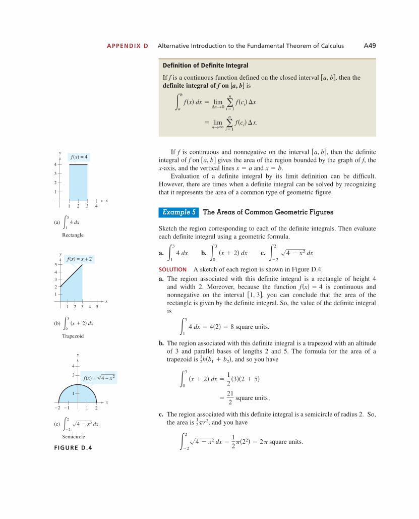
If f is continuous and nonnegative on the interval then the definiteintegral of f on gives the area of the region bounded by the graph of f, the x-axis, and the vertical lines and
Evaluation of a definite integral by its limit definition can be difficult.However, there are times when a definite integral can be solved by recognizingthat it represents the area of a common type of geometric figure.
Example 5 The Areas of Common Geometric Figures
Sketch the region corresponding to each of the definite integrals. Then evaluateeach definite integral using a geometric formula.
a. b. c.
SOLUTION A sketch of each region is shown in Figure D.4.
a. The region associated with this definite integral is a rectangle of height 4 and width 2. Moreover, because the function is continuous and nonnegative on the interval you can conclude that the area of therectangle is given by the definite integral. So, the value of the definite integralis
b. The region associated with this definite integral is a trapezoid with an altitudeof 3 and parallel bases of lengths 2 and 5. The formula for the area of atrapezoid is and so you have
c. The region associated with this definite integral is a semicircle of radius 2. So,the area is and you have
�2
�2
4 � x2 dx �12
��22� � 2� square units.
12�r2,
�212
square units .
�3
0 �x � 2� dx �
12
�3��2 � 5�
12h�b1 � b2�,
�3
1 4 dx � 4�2� � 8 square units.
�1, 3�,f�x� � 4
�2
�2 4 � x2 dx�3
0 �x � 2� dx�3
1 4 dx
x � b.x � a�a, b�
�a, b�,
Definition of Definite Integral
If is a continuous function defined on the closed interval then thedefinite integral of on is
� limn→�
n
i�1 f�ci� �x.
�b
a
f �x� dx � lim�x→0
n
i�1 f�ci� �x
[a, b]f�a, b�,f
x
4
3
2
1
y
1 2 3 4
f (x) = 4
(a)
Rectangle
�3
1 4 dx
x
4
3
5
2
1
y
1 2 3 4 5
f (x) = x + 2
(b)
Trapezoid
�3
0 �x � 2� dx
x
4
3
1
y
−1−2 1 2
f (x) = 4 − x2
(c)
Semicircle
FIGURE D.4
�2
�2 4 � x2 dx
APPENDIX D Alternative Introduction to the Fundamental Theorem of Calculus A49
1053715_App_D.qxp 11/5/08 1:22 PM Page A49

A50 APPENDIX D Alternative Introduction to the Fundamental Theorem of Calculus
For some simple functions, it is possible to evaluate definite integrals by theRiemann sum definition. In the next example, you will use the fact that the sumof the first n integers is given by the formula
See Exercise 29.
to compute the area of the triangular region in Examples 3 and 4.
Example 6 Evaluating a Definite Integral by Its Definition
Evaluate
SOLUTION Let and choose to be the right endpointof each subinterval, Then you have
This limit can be evaluated in the same way that you calculated horizontal asymp-totes in Section 9.3. In particular, as n approaches infinity, you see that approaches 0, and the limit above is 9. So, you can conclude that
From Example 6, you can see that it can be difficult to evaluate the definiteintegral of even a simple function by using Riemann sums. A computer can helpin calculating these sums for large values of n, but this procedure would only givean approximation of the definite integral. Fortunately, the FundamentalTheorem of Calculus provides a technique for evaluating definite integrals usingantiderivatives, and for this reason it is often thought to be the most important theorem in calculus. In the remainder of this appendix, you will see how derivatives and integrals are related via the Fundamental Theorem of Calculus.
To simplify the discussion, assume that f is a continuous nonnegative function defined on the interval Let be the area of the region under thegraph of f from a to x, as indicated in Figure D.5. The area under the shadedregion in Figure D.6 is A�x � �x� � A�x�.
A�x��a, b�.
�3
0 2x dx � 9.
9�n
� limn→�
�9 �9n�.
� limn→�
�18n2��n�n � 1�
2 � � lim
n→� 18n2
n
i�1 i
� limn→�
n
i�1 2�i
3n��
3n�
�3
0 2x dx � lim
�x→0
n
i�1 f�ci��x
ci � 3i�n.ci�x � �b � a��n � 3�n,
�3
0 2x dx.
1 � 2 � . . . � n � n
i�1i �
n�n � 1�2
t
y
a x
y = f(t)
FIGURE D.5
t
y
a x
y = f (t)
x + Δx
FIGURE D.6
1053715_App_D.qxp 11/5/08 1:22 PM Page A50

PROOF From the discussion above, you know that
and in particular
and
If F is any antiderivative of f, then you know that F differs from A by a constant.That is, So
You are now ready to continue Section 11.4, on page 836, just after the statement of the Fundamental Theorem of Calculus.
� F�b� � F�a�. � �F�b� � C� � �F�a� � C�
�b
a
f�x� dx � A�b� � A�a�
A�x� � F�x� � C.
A�b� � �b
a
f�x� dx.
A�a� � �a
a
f�x� dx � 0
�x
a
f�x� dx � A�x�
If is small, then this area is approximated by the area of the rectangle of heightand width So, you have
Dividing by produces
By taking the limit as approaches 0, you can see that
and you can establish the fact that the area function is an antiderivative of f.Although it was assumed that f is continuous and nonnegative, this developmentis valid if the function f is simply continuous on the closed interval Thisresult is used in the proof of the Fundamental Theorem of Calculus.
�a, b�.
A�x�
� A��x�
f�x� � lim�x→0
A�x � �x� � A�x�
�x
�x
f�x� �A�x � �x� � A�x�
�x.
�x
A�x � �x� � A�x� � f�x� �x.
�x.f�x��x
Fundamental Theorem of Calculus
If is a continuous function on the closed interval then
where is any function such that F��x� � f �x�.F
�b
a
f�x�dx � F�b� � F�a�
�a, b�,f
APPENDIX D Alternative Introduction to the Fundamental Theorem of Calculus A51
1053715_App_D.qxp 11/5/08 1:22 PM Page A51
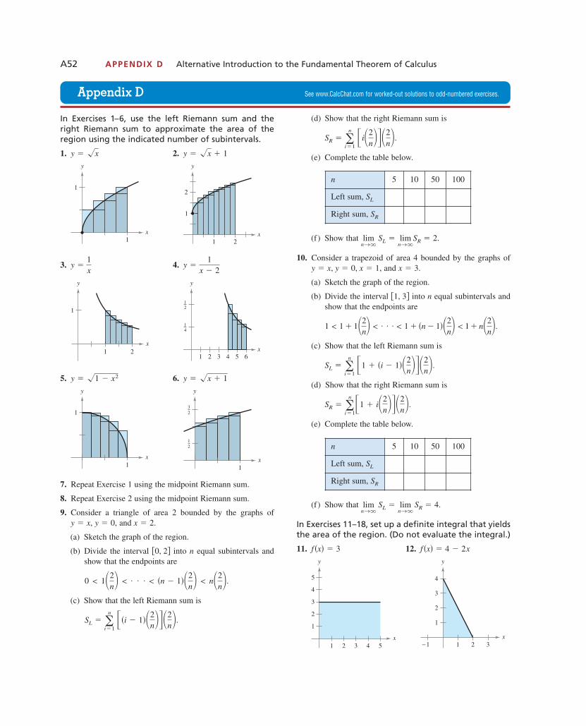
In Exercises 1–6, use the left Riemann sum and theright Riemann sum to approximate the area of theregion using the indicated number of subintervals.
1. 2.
3. 4.
5. 6.
7. Repeat Exercise 1 using the midpoint Riemann sum.
8. Repeat Exercise 2 using the midpoint Riemann sum.
9. Consider a triangle of area 2 bounded by the graphs ofand
(a) Sketch the graph of the region.
(b) Divide the interval into n equal subintervals andshow that the endpoints are
(c) Show that the left Riemann sum is
(d) Show that the right Riemann sum is
(e) Complete the table below.
(f) Show that
10. Consider a trapezoid of area 4 bounded by the graphs ofand
(a) Sketch the graph of the region.
(b) Divide the interval into n equal subintervals andshow that the endpoints are
(c) Show that the left Riemann sum is
(d) Show that the right Riemann sum is
(e) Complete the table below.
(f) Show that
In Exercises 11–18, set up a definite integral that yieldsthe area of the region. (Do not evaluate the integral.)
11. 12.
x
4
3
2
1
y
1 2 3−1x
5
4
3
2
1
y
1 2 3 4 5
f �x� � 4 � 2xf �x� � 3
limn→�
SL � limn→�
SR � 4.
SR � n
i�1�1 � i�2
n��2n�.
SL � n
i�1 �1 � �i � 1��2
n��2n�.
1 < 1 � 1�2n� < . . . < 1 � �n � 1��2
n� < 1 � n�2n�.
�1, 3�
x � 3.y � x, y � 0, x � 1,
limn→�
SL � limn→�
SR � 2.
SR � n
i�1 �i�2
n��2n�.
SL � n
i�1 ��i � 1��2
n��2n�.
0 < 1�2n� < . . . < �n � 1��2
n� < n�2n�.
�0, 2�
x � 2.y � 0,y � x,
x1
y
12
32
x
1
1
y
y � x � 1y � 1 � x2
x
y
12
14
1 2 3 4 5 6
x
1
y
1 2
y �1
x � 2y �
1x
x
1
2
y
1 2
x
1
1
y
y � x � 1y � x
A52 APPENDIX D Alternative Introduction to the Fundamental Theorem of Calculus
Appendix D See www.CalcChat.com for worked-out solutions to odd-numbered exercises.
n 5 10 50 100
Left sum, SL
Right sum, SR
n 5 10 50 100
Left sum, SL
Right sum, SR
1053715_App_D.qxp 11/5/08 1:22 PM Page A52
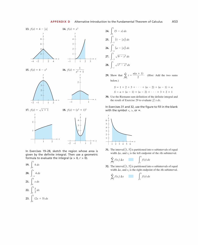
APPENDIX D Alternative Introduction to the Fundamental Theorem of Calculus A53
13. 14.
15. 16.
17. 18.
In Exercises 19–28, sketch the region whose area isgiven by the definite integral. Then use a geometricformula to evaluate the integral
19.
20.
21.
22.
23.
24.
25.
26.
27.
28.
29. Show that (Hint: Add the two sums
below.)
30. Use the Riemann sum definition of the definite integral andthe result of Exercise 29 to evaluate
In Exercises 31 and 32, use the figure to fill in the blankwith the symbol or
31. The interval is partitioned into n subintervals of equalwidth and is the left endpoint of the ith subinterval.
32. The interval is partitioned into n subintervals of equalwidth and is the right endpoint of the ith subinterval.
�5
1 f �x� dx�
n
i�1 f �xi� �x
xi�x,�1, 5�
�5
1 f �x� dx�
n
i�1 f �xi� �x
xi�x,�1, 5�
x1 2 3 4 5 6
6
5
4
3
2
1
y
�.>,<,
�21 x dx.
S � n � �n � 1� � �n � 2� � . . . � 3 � 2 � 1
S � 1 � 2 � 3 � . . . � �n � 2� � �n � 1� � n
n
i�1 i �
n�n � 1�2
.
�r
�r
r2 � x2 dx
�3
�3 9 � x2 dx
�a
�a
�a � �x�� dx
�1
�1 �1 � �x�� dx
�5
0 �5 � x� dx
�2
0 �2x � 5� dx
�4
0 x2
dx
�4
0 x dx
�a
�a
4 dx
�3
0 4 dx
�a > 0, r > 0�.
x
4
3
2
−1−2 1 2
y
x
2
1
1 2
y
f �x� � �x2 � 1�2f �x� � x � 1
x
2
y
−1 1x
3
2
1
y
1 2−1−2
f �x� �1
x2 � 1f �x� � 4 � x2
x
4
3
2
1
y
−1 1 2 3x
8
6
4
2
y
2 4−2−4
f �x� � x2f �x� � 4 � �x�
1053715_App_D.qxp 11/5/08 1:22 PM Page A53

A54 APPENDIX E Formulas
E.1 Differentiation and Integration FormulasUse differentiation and integration tables to supplement differentiation and integration techniques.
E Formulas
Differentiation Formulas
1. 2. 3.
4. 5. 6.
7. 8. 9.
10. 11. 12.
13. 14. 15.
Integration Formulas
Forms Involving
1.
2.
Forms Involving
3.
4.
5.
6.
7. � u2
�a � bu�2 du �1b3 �bu �
a2
a � bu� 2a ln�a � bu�� � C
� u2
a � bu du �
1b3 ��
bu2
�2a � bu� � a2 ln�a � bu� � C
n � 1, 2� u
�a � bu�n du �1b2 � �1
�n � 2��a � bu�n�2 �a
�n � 1��a � bu�n�1 � C,
� u
�a � bu�2 du �1b2 � a
a � bu� ln�a � bu�� � C
� u
a � bu du �
1b2�bu � a ln�a � bu�� � C
a 1 bu
� 1u
du � ln �u� � C
n � �1� un du �un�1
n � 1� C,
un
ddx
csc u� � ��csc u cot u�u�ddx
sec u� � �sec u tan u�u�ddx
cot u� � ��csc2 u�u�
ddx
tan u� � �sec2 u�u�ddx
cos u� � ��sin u�u�ddx
sin u� � �cos u�u�
ddx
eu� � euu�ddx
ln u� �u�
uddx
x� � 1
ddx
un� � nun�1u�ddx
c� � 0ddx�
uv �
vu� � uv�
v2
ddx
uv� � uv� � vu�ddx
u ± v� � u� ± v�ddx
cu� � cu�
1053715_App_E.1_E.2.qxp 11/5/08 1:31 PM Page A54
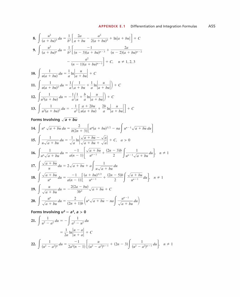
8.
9.
10.
11.
12.
13.
Forms Involving
14.
15.
16.
17.
18.
19.
20.
Forms Involving
21.
22. n � 1� 1
�u2 � a2�n du ��1
2a2�n � 1� �u
�u2 � a2�n�1 � �2n � 3�� 1
�u2 � a2�n�1 du,
�12a
ln�u � au � a� � C
� 1
u2 � a2 du � �� 1
a2 � u2 du
a > 0u2 � a2,
� un
�a � bu du �
2�2n � 1�b �un�a � bu � na�
un�1
�a � bu du�
� u
�a � bu du � �
2�2a � bu�3b2
�a � bu � C
n � 1� �a � bu
un du ��1
a�n � 1� ��a � bu�3 2
un�1 ��2n � 5�b
2 � �a � bu
un�1 du,
� �a � bu
u du � 2�a � bu � a�
1
u�a � bu du
n � 1� 1
un�a � bu du �
�1a�n � 1� ��a � bu
un�1 ��2n � 3�b
2 � 1
un�1�a � bu du,
a > 0� 1
u�a � bu du �
1�a
ln��a � bu � �a�a � bu � �a� � C,
� un �a � bu du �2
b�2n � 3� �un�a � bu�3 2 � na� un�1�a � bu du�a 1 bu
� 1
u2�a � bu�2 du � �1a2 � a � 2bu
u�a � bu� �2ba
ln� ua � bu� � C
� 1u2�a � bu� du � �
1a �
1u
�ba
ln� ua � bu�� � C
� 1
u�a � bu�2 du �1a �
1a � bu
�1a
ln� ua � bu�� � C
� 1
u�a � bu� du �1a
ln� ua � bu� � C
n � 1, 2, 3�a2
�n � 1��a � bu�n�1 � C,
� u2
�a � bu�n du �1b3 � �1
�n � 3��a � bu�n�3 �2a
�n � 2��a � bu�n�2
� u2
�a � bu�3 du �1b3 � 2a
a � bu�
a2
2�a � bu�2 � ln�a � bu� � C
APPENDIX E.1 Differentiation and Integration Formulas A55
1053715_App_E.1_E.2.qxp 11/5/08 1:31 PM Page A55
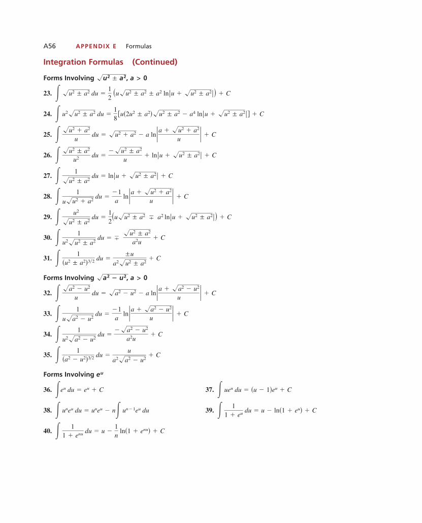
Integration Formulas (Continued)
Forms Involving
23.
24.
25.
26.
27.
28.
29.
30.
31.
Forms Involving
32.
33.
34.
35.
Forms Involving
36. 37.
38. 39.
40. � 1
1 � enu du � u �1n
ln�1 � enu� � C
� 1
1 � eu du � u � ln�1 � eu� � C� uneu du � uneu � n� un�1eu du
� ueu du � �u � 1�eu � C�eu du � eu � C
eu
� 1
�a2 � u2�3 2 du �u
a2�a2 � u2� C
� 1
u2�a2 � u2 du �
��a2 � u2
a2u� C
� 1
u�a2 � u2 du �
�1a
ln�a � �a2 � u2
u � � C
� �a2 � u2
u du � �a2 � u2 � a ln�a � �a2 � u2
u � � C
a > 0�a2 � u2,
� 1
�u2 ± a2�3 2 du �±u
a2�u2 ± a2� C
� 1
u2�u2 ± a2 du � �
�u2 ± a2
a2u� C
� u2
�u2 ± a2 du �
12
�u�u2 ± a2 � a2 ln�u � �u2 ± a2�� � C
� 1
u�u2 � a2 du �
�1a
ln�a � �u2 � a2
u � � C
� 1
�u2 ± a2 du � ln�u � �u2 ± a2� � C
� �u2 ± a2
u2 du ���u2 ± a2
u� ln�u � �u2 ± a2� � C
� �u2 � a2
u du � �u2 � a2 � a ln�a � �u2 � a2
u � � C
� u2�u2 ± a2 du �18
u�2u2 ± a2��u2 ± a2 � a4 ln�u � �u2 ± a2�� � C
� �u2 ± a2 du �12
�u�u2 ± a2 ± a2 ln�u � �u2 ± a2�� � C
a > 0�u2 ± a2,
A56 APPENDIX E Formulas
1053715_App_E.1_E.2.qxp 11/5/08 1:31 PM Page A56

Forms Involving In u
41. 42.
43.
44. 45.
Forms Involving sin u or cos u
46. 47.
48. 49.
50.
51.
52. 53.
54. 55.
56. 57.
58.
Forms Involving tan u, cot u, sec u, or csc u
59. 60.
61. 62.
63. 64.
65. 66.
67.
68.
69. n � 1� secn u du �secn�2 u tan u
n � 1�
n � 2n � 1
� secn�2 u du,
n � 1� cotn u du � �cotn�1 un � 1
� � cotn�2 u du,
n � 1� tann u du �tann�1 un � 1
� � tann�2 u du,
� csc2 u du � �cot u � C� sec2 u du � tan u � C
� cot2 u du � �u � cot u � C� tan2 u du � �u � tan u � C
� csc u du � ln�csc u � cot u� � C� sec u du � ln�sec u � tan u� � C
� cot u du � ln�sin u� � C� tan u du � �ln�cos u� � C
� 1
sin u cos u du � ln�tan u� � C
� 1
1 ± cos u du � �cot u ± csc u � C�
11 ± sin u
du � tan u � sec u � C
� un cos u du � un sin u � n� un�1 sin u du� un sin u du � �un cos u � n� un�1 cos u du
� u cos u du � cos u � u sin u � C� u sin u du � sin u � u cos u � C
� cosn u du �cosn�1 u sin u
n�
n � 1n
� cosn�2 u du
� sinn u du � �sinn�1 u cos u
n�
n � 1n
� sinn�2 u du
� cos2 u du �12
�u � sin u cos u� � C� sin2 u du �12
�u � sin u cos u� � C
� cos u du � sin u � C� sin u du � �cos u � C
� �ln u�n du � u�ln u�n � n � �ln u�n�1 du� �ln u�2 du � u2 � 2 ln u � �ln u�2� � C
n � �1� un ln u du �un�1
�n � 1�2 �1 � �n � 1� ln u� � C,
�u ln u du �u2
4 ��1 � 2 ln u� � C� ln u du � u��1 � ln u� � C
APPENDIX E.1 Differentiation and Integration Formulas A57
1053715_App_E.1_E.2.qxp 11/5/08 1:31 PM Page A57

A58 APPENDIX E Formulas
70.
71.
72.
73.
74. � 1
1 ± csc u du � u � tan u ± sec u � C
� 1
1 ± sec u du � u � cot u � csc u � C
� 1
1 ± cot u du �
12
�u � ln�sin u ± cos u�� � C
� 1
1 ± tan u du �
12
�u ± ln�cos u ± sin u�� � C
n � 1� cscn u du � �cscn�2 u cot u
n � 1�
n � 2n � 1
� cscn�2 u du,
Formulas from Business
Basic Terms
number of units produced (or sold)
price per unit
total revenue from selling x units
total cost of producing x units
average cost per unit
total profit from selling x units
Basic Equations
Typical Graphs of Supply and Demand Curves
Supply curves increase as price increases and demand curves decrease as price increases. The equilibrium point occurs when the supply and demand curves intersect.
x
Demand
Equilibrium point(x0, p0)
Supply
x0
p0
Equilibrium quantity
Equilibriumprice
p
P � R � CC �Cx
R � xp
P �
C �
C �
R �
p �
x �
E.2 Formulas from Business and FinanceSummary of business and finance formulas
1053715_App_E.1_E.2.qxp 11/5/08 1:31 PM Page A58
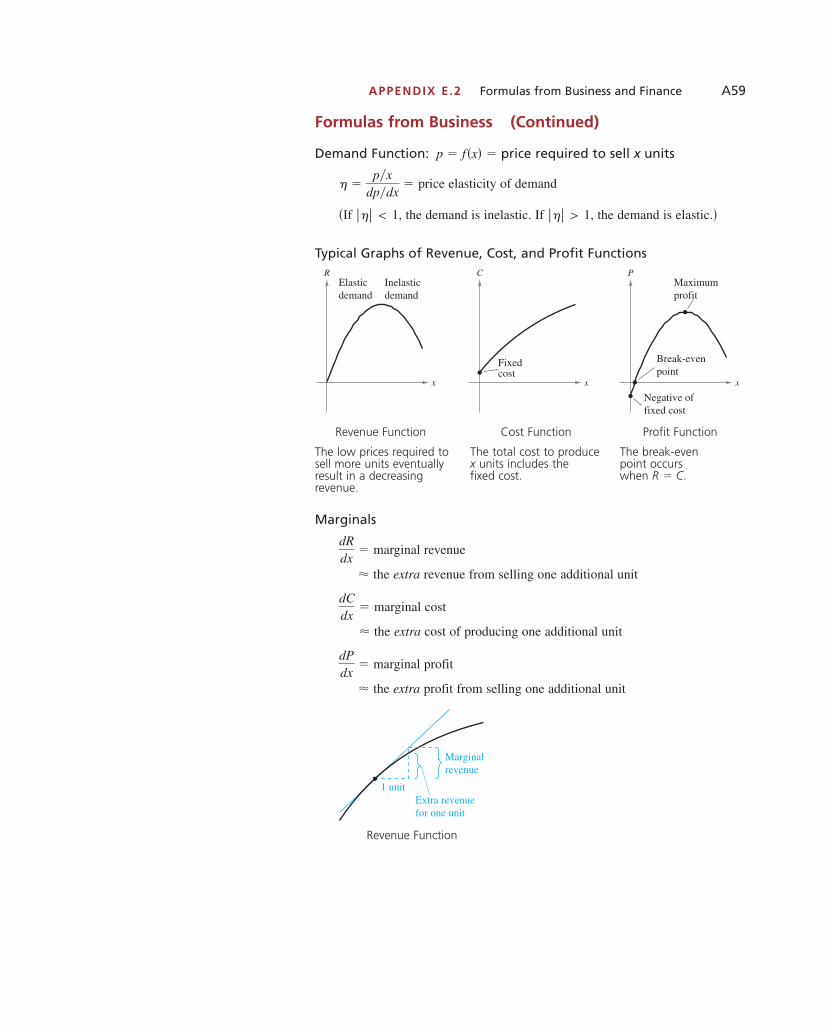
APPENDIX E.2 Formulas from Business and Finance A59
Formulas from Business (Continued)
Demand Function: price required to sell x units
price elasticity of demand
If the demand is inelastic. If the demand is elastic.
Typical Graphs of Revenue, Cost, and Profit Functions
Marginals
marginal revenue
the extra revenue from selling one additional unit
marginal cost
the extra cost of producing one additional unit
marginal profit
the extra profit from selling one additional unit
Revenue Function
1 unitExtra revenuefor one unit
Marginalrevenue
�
dPdx
�
�
dCdx
�
�
dRdx
�
Maximumprofit
x
Negative offixed cost
Break-evenpoint
P
x
Fixedcost
CInelasticdemand
x
Elasticdemand
R
���� > 1,��� < 1,�
� �p x
dp dx�
p � f�x� �
Revenue Function Cost Function Profit Function
The low prices required tosell more units eventuallyresult in a decreasing revenue.
The total cost to producex units includes the fixed cost.
The break-even point occurs when R � C.
1053715_App_E.1_E.2.qxp 11/5/08 1:31 PM Page A59
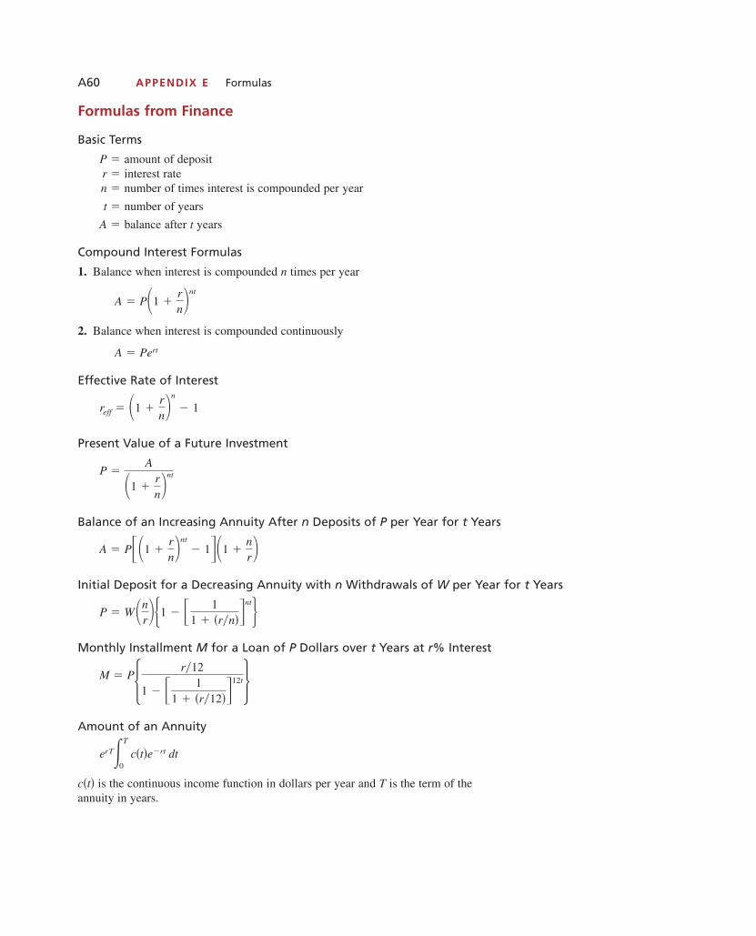
A60 APPENDIX E Formulas
Formulas from Finance
Basic Terms
amount of depositinterest ratenumber of times interest is compounded per year
number of years
balance after t years
Compound Interest Formulas
1. Balance when interest is compounded n times per year
2. Balance when interest is compounded continuously
Effective Rate of Interest
Present Value of a Future Investment
Balance of an Increasing Annuity After n Deposits of P per Year for t Years
Initial Deposit for a Decreasing Annuity with n Withdrawals of W per Year for t Years
Monthly Installment M for a Loan of P Dollars over t Years at r% Interest
Amount of an Annuity
is the continuous income function in dollars per year and T is the term of theannuity in years.c�t�
erT�T
0 c�t�e�rt dt
M � P� r 12
1 � � 11 � �r 12�
12t�
P � W�nr��1 � � 1
1 � �r n�nt�
A � P��1 �rn�
nt
� 1�1 �nr�
P �A
�1 �rn�
nt
reff � �1 �rn�
n
� 1
A � Pert
A � P�1 �rn�
nt
A �
t �
n � r � P �
1053715_App_E.1_E.2.qxp 11/5/08 1:31 PM Page A60
APPENDIX F.1 Solutions of Differential Equations A61
F.1 Solutions of Differential EquationsFind general solutions of differential equations. • Find particular solutions of differential equations.
F Differential Equations
General Solution of a Differential Equation
A differential equation is an equation involving a differentiable function andone or more of its derivatives. For instance,
Differential equation
is a differential equation. A function is a solution of a differential equation if the equation is satisfied when y and its derivatives are replaced by and its derivatives. For instance,
Solution of differential equation
is a solution of the differential equation shown above. To see this, substitute for yand in the original equation.
Substitute for y and
In the same way, you can show that and arealso solutions of the differential equation. In fact, each function given by
General solution
where C is a real number, is a solution of the equation. This family of solutionsis called the general solution of the differential equation.
Example 1 Checking Solutions
Show that
a. and b.
are solutions of the differential equation
SOLUTION
a. Because and it follows that
So, is a solution.
b. Because and it follows that
So, is also a solution.y � Ce�x
� 0.
y� � y � Ce�x � Ce�x
y� � Ce�x,y� � �Ce�x
y � Cex
� 0.
y� � y � Ce x � Ce x
y� � Cex,y� � Cex
y� � y � 0.
y � Ce�xy � Cex
y � Ce�2x
y �12e�2xy � 2e�2x, y � �3e�2x,
� 0
y�. y� � 2y � �2e�2x � 2�e�2x�
y� � �2e�2x
y � e�2x
f�x�y � f�x�
y� � 2y � 0
1053715_App_F01.qxp 11/5/08 1:23 PM Page A61

A62 APPENDIX F Differential Equations
Particular Solutions and Initial Conditions
A particular solution of a differential equation is any solution that is obtainedby assigning specific values to the constants in the general equation.*
Geometrically, the general solution of a differential equation is a family ofgraphs called solution curves. For instance, the general solution of the differen-tial equation is
General solution
Figure F.1 shows several solution curves of this differential equation.Particular solutions of a differential equation are obtained from initial
conditions placed on the unknown function and its derivatives. For instance,in Figure F.1, suppose you want to find the particular solution whose graph passes through the point This initial condition can be written as
when Initial condition
Substituting these values into the general solution produces whichimplies that So, the particular solution is
Particular solution
Example 2 Finding a Particular Solution
Verify that
General solution
is a solution of the differential equation for any value of C. Thenfind the particular solution determined by the initial condition
when Initial condition
SOLUTION The derivative of is Substituting into thedifferential equation produces
So, is a solution for any value of C. To find the particular solution,substitute and into the general solution to obtain
or
This implies that the particular solution is
Particular solutiony � �227
x3.
C � �227
.2 � C��3�3
y � 2x � �3y � Cx3
� 0.
xy� � 3y � x�3Cx2� � 3�Cx3�
y� � 3Cx2.y � Cx3
x � �3.y � 2
xy� � 3y � 0
y � Cx3
y � 3x2.
C � 3.3 � C�1�2,
x � 1.y � 3
�1, 3�.
y � Cx2.
xy� � 2y � 0
*Some differential equations have solutions other than those given by their general solutions. Theseare called singular solutions. In this brief discussion of differential equations, singular solutions willnot be discussed.
−3
−2
3
2
1
32−2−3
y
x
y = Cx2
(1, 3)
FIGURE F.1
1053715_App_F01.qxp 11/5/08 1:23 PM Page A62
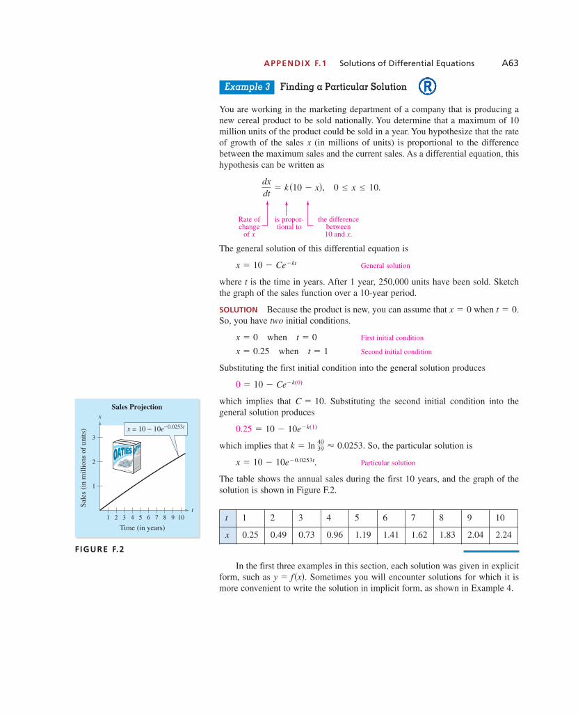
Example 3 Finding a Particular Solution
You are working in the marketing department of a company that is producing anew cereal product to be sold nationally. You determine that a maximum of 10million units of the product could be sold in a year. You hypothesize that the rateof growth of the sales x (in millions of units) is proportional to the differencebetween the maximum sales and the current sales. As a differential equation, thishypothesis can be written as
The general solution of this differential equation is
General solution
where t is the time in years. After 1 year, 250,000 units have been sold. Sketchthe graph of the sales function over a 10-year period.
SOLUTION Because the product is new, you can assume that when So, you have two initial conditions.
when First initial condition
when Second initial condition
Substituting the first initial condition into the general solution produces
which implies that Substituting the second initial condition into the general solution produces
which implies that So, the particular solution is
Particular solution
The table shows the annual sales during the first 10 years, and the graph of thesolution is shown in Figure F.2.
In the first three examples in this section, each solution was given in explicitform, such as Sometimes you will encounter solutions for which it ismore convenient to write the solution in implicit form, as shown in Example 4.
y � f�x�.
x � 10 � 10e�0.0253t.
k � ln 4039 � 0.0253.
0.25 � 10 � 10e�k(1)
C � 10.
0 � 10 � Ce�k(0)
t � 1x � 0.25
t � 0x � 0
t � 0.x � 0
x � 10 � Ce�kt
0 ≤ x ≤ 10.dxdt
� k�10 � x�,
Rate ofchange
of x
is propor-tional to
the differencebetween 10 and x.
3
2
1
x
t
x = 10 − 10e−0.0253t
Sales Projection
Time (in years)
Sale
s (i
n m
illio
ns o
f un
its)
1 2 3 4 5 6 7 8 9 10
FIGURE F.2
t 1 2 3 4 5 6 7 8 9 10
x 0.25 0.49 0.73 0.96 1.19 1.41 1.62 1.83 2.04 2.24
APPENDIX F.1 Solutions of Differential Equations A63
1053715_App_F01.qxp 11/5/08 1:23 PM Page A63

A64 APPENDIX F Differential Equations
Example 4 Sketching Graphs of Solutions
Verify that
General solution
is a solution of the differential equation
Then sketch the particular solutions represented by and
SOLUTION To verify the given solution, differentiate each side with respect to x.
Given general solution
Differentiate with respect to x.
Divide each side by 2.
Because the third equation is the given differential equation, you can concludethat
is a solution. The particular solutions represented by and are shown in Figure F.3.
FIGURE F.3 Graphs of Five Particular Solutions
22
2
3
2
2
2
2
3
1
y
x
x
y
x
y
x
x
C = 0
C = 1
C = −1 C = −4
y y
C = 4
C � ± 4C � ±1,C � 0,
2y2 � x2 � C
2yy� � x � 0
4yy� � 2x � 0
2y2 � x2 � C
C � ±4.C � 0, C � ±1,
2yy� � x � 0.
2y2 � x2 � C
1. Complete the following: A ________ equation is an equation involving adifferentiable function and one or more of its derivatives.
2. Complete the following: Because each function given by is a solution of is the ________ solution of
3. Explain why is a differential equation.
4. In general, describe in words a particular solution of a differential equation.
y� � 3y � 0
y� 1 2y � 0.y � Ce�2xy� 1 2y � 0,
y � Ce�2x
C O N C E P T C H E C K
1053715_App_F01.qxp 11/5/08 1:23 PM Page A64

APPENDIX F.1 Solutions of Differential Equations A65
In Exercises 1–10, verify that the function is a solutionof the differential equation.
Solution Differential Equation
1.
2.
3.
4.
5.
6.
7.
8.
9.
10.
In Exercises 11–28, verify that the function is a solutionof the differential equation for any value of
Solution Differential Equation
11.
12.
13.
14.
15.
16.
17.
18.
19.
20. y� � y� � 0y � C1 � C2ex
xy� � y � x�3x � 4�y � x2 � 2x �Cx
y� �yx
� 2 � �xy � x ln x2 � 2x3�2 � Cx
xy� � 3x � 2y � 0y � Cx2 � 3x
y� � y � 10 � 0y � Ce�t � 10
3 dydt
� y � 7 � 0y � Ce�t�3 � 7
dydx
� �4yy � Ce�4x
dydx
� 4yy � Ce 4x
dydx
� �x
�4 � x2y � �4 � x2 � C
dydx
� �1x2y �
1x
� C
C.
y� � 3x2y� � 6xy � 0y � e x3
y� � y� � 2y � 0y � 2e2x
xy� � 2y� � 0y �1x
x 2y� � 2y � 0y � x2
y� �2x
y � 0y � 4x2
y� �3x
y � 0y � 2x3
y� � 2xy � 0y � 3e x2
y� � 2y � 0y � e�2x
y� � 6x2 � 1y � 2x3 � x � 1
y� � 3x2y � x3 � 5
The following warm-up exercises involve skills that were covered in earlier sections. You willuse these skills in the exercise set for this section. For additional help, review Sections 8.1, 8.2,and 10.4.
In Exercises 1–4, find the first and second derivatives of the function.
1.
2.
3.
4.
In Exercises 5–8, use implicit differentiation to find
5.
6.
7.
8.
In Exercises 9 and 10, solve for
9.
10. 14.75 � 25 � 25e�2k
0.5 � 9 � 9e�k
k.
3xy � x2y 2 � 10
xy 2 � 3
2x � y3 � 4y
x2 � y 2 � 2x
dy/dx.
y � �3e x2
y � �3e2x
y � �2x3 � 8x � 4
y � 3x2 � 2x � 1
Skills Review F.1
Exercises F.1 See www.CalcChat.com for worked-out solutions to odd-numbered exercises.
1053715_App_F01.qxp 11/5/08 1:23 PM Page A65

A66 APPENDIX F Differential Equations
Solution Differential Equation
21.
22.
23.
24.
25.
26.
27.
28.
In Exercises 29–32, use implicit differentiation to verifythat the function is a solution of the differential equation for any value of
Solution Differential Equation
29.
30.
31.
32.
In Exercises 33–36, determine whether the function isa solution of the differential equation
33.
34.
35.
36.
In Exercises 37–40, determine whether the function isa solution of the differential equation
37.
38.
39.
40.
In Exercises 41–48, verify that the general solution satisfies the differential equation. Then find the particular solution that satisfies the initial condition.
41. General solution:Differential equation:Initial condition: when
42. General solution:Differential equation:Initial condition: when
43. General solution:Differential equation:Initial condition: and when
44. General solution:Differential equation:Initial condition: and when
45. General solution:Differential equation:Initial condition: and when
46. General solution:Differential equation:Initial condition: when
47. General solution:Differential equation:Initial condition: when
when
48. General solution:
Differential equation:
Initial condition: and when
In Exercises 49–52, the general solution of the differ-ential equation is given. Use a graphing utility tograph the particular solutions that correspond to theindicated values of
General Solution Differential Equation C-Values
49. 1, 2, 4
50.
51.
52.
In Exercises 53–60, use integration to find the generalsolution of the differential equation.
53.
54.
55.
56.
57.
58.
59.
60.dydx
� xex
dydx
� x�x � 3
dydx
�x
1 � x2
dydx
�1
x2 � 1
dydx
�x � 2
x
dydx
�x � 3
x
dydx
�1
1 � x
dydx
� 3x2
0, ±1, ±2y� � y � 0y � Ce�x
0, ±1, ±2�x � 2�y� � 2y � 0y � C�x � 2�2
0, ±1, ±44yy� � x � 04y 2 � x2 � C
xy� � 2y � 0y � Cx2
C.
x � 0y� � 1y � 2
y� � 4y� � 4y � x 2e2x
y � �C1 � C2 x �112 x 4�e2x
x � 3y � 0x � 0y � 4
9y� � 12y� � 4y � 0y � e2x�3�C1 � C2 x�
x � 1y � 2y� � �2x � 1�y � 0
y � Ce x�x2
x � 0y� � 6y � 5y� � y� � 12y � 0
y � C1e4x � C2e
�3x
x � 2y� � 4y � 0x 2y� � 3xy� � 3y � 0
y � C1x � C2 x3
x � 1y� � 0.5y � 5xy� � y� � 0
y � C1 � C2 ln x
x � 1y � 22x � 3yy� � 0
2x2 � 3y 2 � C
x � 0y � 3y� � 2y � 0
y � Ce�2x
y � x ln x
y � xe x
y � 4e x �29 xe�2x
y �29 xe�2x
y�� � 3y� 1 2y � 0.
y � 4e2x
y �4x
y � 5 ln x
y � e�2x
y �4� � 16y � 0.
y3y� � x2 � y 2 � 0x2 � y 2 � C
x2y� � 2�x � y� � 0x2 � xy � C
�x � y�y� � x � y � 0y 2 � 2xy � x2 � C
y� �2xy
x2 � y 2x2 � y 2 � Cy
C.
x � y � xy� � 0y � x�ln x � C�x�y� � 1� � �y � 4� � 0y � x ln x � Cx � 4
y� � �2x � 1�y � 0y � Ce x�x2
y� � 2xy � xy 2y �2
1 � Ce x2
2xy� � y � x3 � xy �x3
5� x � C�x
y� �ayx
� bx3y �bx 4
4 � a� Cx a
y� � 3y� � 4y � 0y � C1e4x � C2e
�x
2y� � 3y� � 2y � 0y � C1ex�2 � C2e
�2x
1053715_App_F01.qxp 11/5/08 1:23 PM Page A66

In Exercises 61–64, some of the curves corresponding todifferent values of in the general solution of the differential equation are given. Find the particular solu-tion that passes through the point shown on the graph.
61. 62.
63. 64.
65. Biology The limiting capacity of the habitat of a wildlifeherd is 750. The growth rate of the herd is propor-tional to the unutilized opportunity for growth, as describedby the differential equation
The general solution of this differential equation is
When the population of the herd is 100. After 2 years, the population has grown to 160.
(a) Write the population function as a function of
(b) Use a graphing utility to graph the population function.
(c) What is the population of the herd after 4 years?
66. Investment The rate of growth of an investment isproportional to the amount in the investment at any time That is,
The initial investment is $1000, and after 10 years thebalance is $3320.12. The general solution is
What is the particular solution?
67. Marketing You are working in the marketing depart-ment of a computer software company. Your marketingteam determines that a maximum of 30,000 units of a newproduct can be sold in a year. You hypothesize that the rateof growth of the sales is proportional to the differencebetween the maximum sales and the current sales. That is,
The general solution of this differential equation is
where is the time in years. During the first year, 2000 unitsare sold. Complete the table showing the numbers of unitssold in subsequent years.
68. Marketing In Exercise 67, suppose that the maximumannual sales are 50,000 units. How does this change thesales shown in the table?
69. Safety Assume that the rate of change per hour in thenumber of miles of road cleared by a snowplow isinversely proportional to the depth of the snow. This rateof change is described by the differential equation
Show that
is a solution of this differential equation.
70. Show that is a solution of the differen-tial equation
where is a constant.
71. The function is a solution of the differential equation
Is it possible to determine or from the informationgiven? If so, find its value.
True or False? In Exercises 72 and 73, determinewhether the statement is true or false. If it is false,explain why or give an example that shows it is false.
72. A differential equation can have more than one solution.
73. If is a solution of a differential equation, thenis also a solution.y � f �x� � C
y � f �x�
kC
dydx
� 0.07y.
y � Cekx
k
y � a � b� y � a� � 1k dy
dt
y � a � Ce k�1�b�t
s � 25 �13
ln 3 ln
h2
dsdh
�kh
.
hs
t
x � 30,000 � Ce�kt
dxdt
� k�30,000 � x�.
x
A � Cekt.
dAdt
� kA.
t.
t.N
t � 0,
N � 750 � Ce�kt.
dNdt
� k�750 � N �.
dN�dt
1
2
−1
−2
x
(2, 1)y
1 2 3−1−2−3
456
x
(0, 3)
y
2xy� � y � 0y� � y � 0
y 2 � 2Cxy � Cex
432
−4−3
43−3x
(3, 4)
y
7
−4−3−2−1
4321
654x
(4, 4)
y
yy� � 2x � 02xy� � 3y � 0
2x2 � y 2 � Cy 2 � Cx3
C
Year, t 2 4 6 8 10
Units, x
APPENDIX F.1 Solutions of Differential Equations A67
1053715_App_F01.qxp 11/5/08 1:24 PM Page A67

A68 APPENDIX F Differential Equations
F.2 Separation of VariablesUse separation of variables to solve differential equations. • Use differential equations to model and solve real-life problems.
Separation of Variables
The simplest type of differential equation is one of the form You knowthat this type of equation can be solved by integration to obtain
In this section, you will learn how to use integration to solve another importantfamily of differential equations—those in which the variables can be separated.This technique is called separation of variables.
Essentially, the technique of separation of variables is just what its nameimplies. For a differential equation involving x and y, you separate the x variablesto one side and the y variables to the other. After separating variables, integrateeach side to obtain the general solution. Here is an example.
Example 1 Solving a Differential Equation
Find the general solution of
SOLUTION Begin by separating variables, then integrate each side.
Differential equation
Separate variables.
Integrate each side.
General solution y3
3� y �
x2
2� C
��y2 � 1� dy � �x dx
(y2 � 1� dy � x dx
dydx
�x
y2 � 1
dydx
�x
y2 � 1.
y � � f �x� dx.
y� � f �x�.
Separation of Variables
If and are continuous functions, then the differential equation
has a general solution of
� 1
g�y� dy � � f �x� dx � C.
dydx
� f �x�g�y�
gf
You can use a symbolicintegration utility to solve
a separable variables differentialequation. Use a symbolic integration utility to solve thedifferential equation
y� �x
y2 � 1.
T E C H N O L O G Y
1053715_App_F02.qxp 11/5/08 1:24 PM Page A68
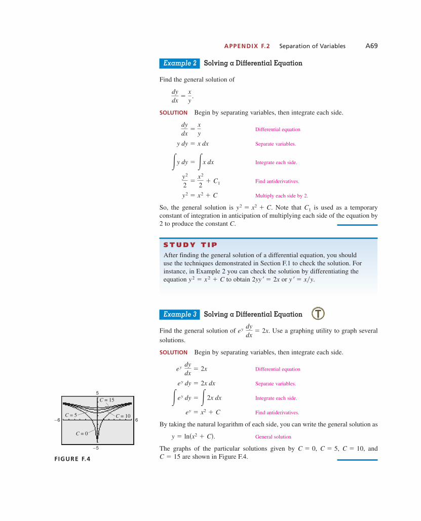
APPENDIX F.2 Separation of Variables A69
Example 2 Solving a Differential Equation
Find the general solution of
SOLUTION Begin by separating variables, then integrate each side.
Differential equation
Separate variables.
Integrate each side.
Find antiderivatives.
Multiply each side by 2.
So, the general solution is Note that is used as a temporaryconstant of integration in anticipation of multiplying each side of the equation by2 to produce the constant C.
Example 3 Solving a Differential Equation
Find the general solution of Use a graphing utility to graph several
solutions.
SOLUTION Begin by separating variables, then integrate each side.
Differential equation
Separate variables.
Integrate each side.
Find antiderivatives.
By taking the natural logarithm of each side, you can write the general solution as
General solution
The graphs of the particular solutions given by andare shown in Figure F.4.C � 15
C � 10,C � 5,C � 0,
y � ln�x2 � C�.
ey � x2 � C
�ey dy � � 2x dx
ey dy � 2x dx
ey dydx
� 2x
ey dydx
� 2x.
C1y2 � x2 � C.
y2 � x2 � C
y2
2�
x2
2� C1
�y dy � �x dx
y dy � x dx
dydx
�xy
dydx
�xy
.
S T U D Y T I PAfter finding the general solution of a differential equation, you should use the techniques demonstrated in Section F.1 to check the solution. Forinstance, in Example 2 you can check the solution by differentiating theequation to obtain or y� � x�y.2yy� � 2xy2 � x2 � C
−5
6−6
5
C = 0
C = 5 C = 10
C = 15
FIGURE F.4
1053715_App_F02.qxp 11/5/08 1:24 PM Page A69

A70 APPENDIX F Differential Equations
Example 4 Finding a Particular Solution
Solve the differential equation
subject to the initial condition when
SOLUTION
Differential equation
Subtract from each side.
Separate variables.
Integrate each side.
Find antiderivatives.
Multiply each side by 2.
To find the particular solution, substitute the initial condition values to obtain
This implies that or So, the particular solution that satisfiesthe initial condition is
Particular solution
Example 5 Solving a Differential Equation
Example 3 in Section F.1 uses the differential equation
to model the sales of a new product. Solve this differential equation.
SOLUTION
Differential equation
Separate variables.
Integrate each side.
Find antiderivatives.
Multiply each side by
Exponentiate each side.
Solve for x. x � 10 � Ce�kt
10 � x � e�kt�C1
�1. ln�10 � x� � �kt � C1
�ln�10 � x� � kt � C1
� 110 � x
dx � �k dt
1
10 � x dx � k dt
dxdt
� k�10 � x�
dxdt
� k�10 � x�
y2 � �ex2� 2.
C � 2.1 � �1 � C,
�1�2 � �e�0�2� C.
y2 � �ex2� C
y2
2� �
12
ex2� C1
�y dy � ��xex2 dx
y dy � �xex2 dx
xex2 y dydx
� �xex2
xex2� yy� � 0
x � 0.y � 1
xex2� yy� � 0
S T U D Y T I PIn Example 5, the context of the original model indicates that is positive. So,when you integrate you can write rather than
Also note in Example 5 that the solution agrees with the one that was given inExample 3 in Section F.1.
�ln�10 � x�.�ln�10 � x�,
1��10 � x�,�10 � x�
1053715_App_F02.qxp 11/5/08 1:24 PM Page A70

Applications
Example 6 Modeling National Income
Let y represent the national income, let a represent the income spent on necessi-ties, and let b represent the percent of the remaining income spent on luxuries. Acommonly used economic model that relates these three quantities is
where t is the time in years. Assume that b is 75%, and solve the resulting differ-ential equation.
SOLUTION Because b is 75%, it follows that is 0.25. So, you can solvethe differential equation as shown.
Differential equation
Separate variables.
Integrate each side.
Find antiderivatives, given
Exponentiate each side.
Add a to each side.
The graph of this solution is shown in Figure F.5. In the figure, note that thenational income is spent in three ways.
FIGURE F.5
Modeling National Income
t
y
a
C
Income consumed onnecessities and luxuries
= + 0.75y a Ce0.25kt
National income= +y a Ce0.25kt
Capital investmentConsumed on luxuriesConsumed on necessities
1 2 3 4 5 6 7 8 9 10 11 12 13 14
Time (in years)
�National income� � �necessities� � �luxuries� � �capital investment�
y � a � Ce0.25kt
y � a � Ce0.25kt
y � a > 0. ln�y � a� � 0.25kt � C1
� 1y � a
dy � �0.25k dt
1
y � a dy � 0.25k dt
dydt
� k�0.25��y � a�
�1 � b�
dydt
� k�1 � b��y � a�
Corporate profits in the United Statesare closely monitored by New YorkCity’s Wall Street executives. Corporateprofits, however, represent only about12.4% of the national income. In 2005,the national income was more than$10.9 trillion. Of this, about 65.3% was employee compensation.
APPENDIX F.2 Separation of Variables A71
1053715_App_F02.qxp 11/5/08 1:24 PM Page A71
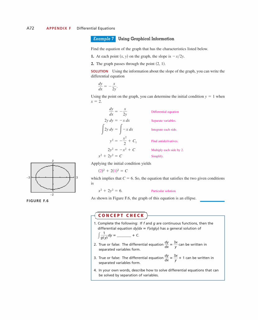
A72 APPENDIX F Differential Equations
Example 7 Using Graphical Information
Find the equation of the graph that has the characteristics listed below.
1. At each point on the graph, the slope is
2. The graph passes through the point
SOLUTION Using the information about the slope of the graph, you can write thedifferential equation
Using the point on the graph, you can determine the initial condition when
Differential equation
Separate variables.
Integrate each side.
Find antiderivatives.
Multiply each side by 2.
Simplify.
Applying the initial condition yields
which implies that So, the equation that satisfies the two given conditionsis
Particular solution
As shown in Figure F.6, the graph of this equation is an ellipse.
x2 � 2y2 � 6.
C � 6.
�2�2 � 2�1�2 � C
x2 � 2y2 � C
2y2 � �x2 � C
y2 � �x2
2� C1
�2y dy � ��x dx
2y dy � �x dx
dydx
� �x2y
x � 2.y � 1
dydx
� �x2y
.
�2, 1�.
�x�2y.�x, y�
−2
3−3
2
FIGURE F.6
1. Complete the following: If and are continuous functions, then thedifferential equation has a general solution of
2. True or false: The differential equation can be written in separated variables form.
3. True or false: The differential equation can be written inseparated variables form.
4. In your own words, describe how to solve differential equations that canbe solved by separation of variables.
dydx
�3xy
1 1
dydx
�3xy
� 1g�y� dy � ________ 1 C.
dy/dx � f �x�g�y�gf
C O N C E P T C H E C K
1053715_App_F02.qxp 11/5/08 1:24 PM Page A72
APPENDIX F.2 Separation of Variables A73
In Exercises 1–6, decide whether the variables in thedifferential equation can be separated.
1. 2.
3. 4.
5. 6.
In Exercises 7–26, use separation of variables to findthe general solution of the differential equation.
7. 8.
9. 10.
11. 12.
13. 14.
15. 16.
17. 18.
19. 20.
21. 22.
23. 24.
25. 26.
In Exercises 27–32, use the initial condition to find theparticular solution of the differential equation.
Differential Equation Initial Condition
27.
28.
29.
30.
31.
32. T � 140 when t � 0dT � k�T � 70� dt � 0
P � 5 when t � 0dP � 6P dt � 0
y � 3 when x � 0dydx
� x2�1 � y�
y � �5 when x � 0x�y � 4� � y� � 0
y � 4 when x � 1x � y y� � 0
y � 4 when x � 0yy� � ex � 0
yy� � 2xex � 0ex�y� � 1� � 1
dydx
�x2 � 2
3y2y� �xy
�x
1 � y
y� � y�x � 1� � 0xy� � y
y� � �2x � 1��y � 3��2 � x�y� � 2y
dydx
�xy
dydx
� 1 � y
e y dydt
� 3t2 � 1dydt
�et
4y
y� � y � 5y� � xy � 0
�1 � y� dydx
� 4x � 0�y � 1� dydx
� 2x
dydx
� x2y3y2 dydx
� 1
dydx
�1x
dydx
� 2x
x dydx
�1y
dydx
� x � y
dydx
�x
x � ydydx
�1x
� 1
dydx
�x � 1
xdydx
�x
y � 3
The following warm-up exercises involve skills that were covered in earlier sections. You willuse these skills in the exercise set for this section. For additional help, review Sections 10.2,11.2, and 11.3.
In Exercises 1–6, find the indefinite integral and check your result by differentiating.
1.
2.
3.
4.
5.
6.
In Exercises 7–10, solve the equation for or
7. 8.
9. 10. �6�2 � 3�6� � e�k10 � 2e2k
��1�2 � ��2�2 � C�3�2 � 6�3� � 1 � C
k.C
�xe1�x2 dx
�e2y dy
� y2y 2 � 1
dy
� 2x � 5
dx
��t 3 � t 1�3� dt
� x 3�2 dx
Skills Review F.2
Exercises F.2 See www.CalcChat.com for worked-out solutions to odd-numbered exercises.
1053715_App_F02.qxp 11/5/08 1:24 PM Page A73
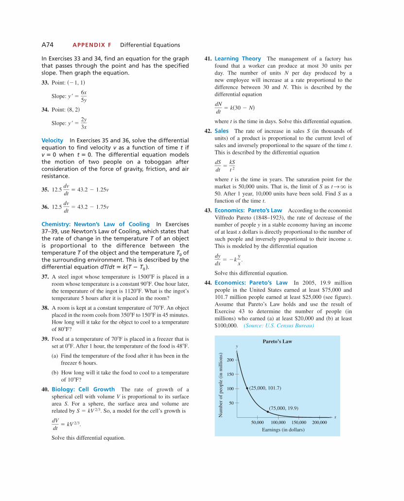
A74 APPENDIX F Differential Equations
In Exercises 33 and 34, find an equation for the graphthat passes through the point and has the specifiedslope. Then graph the equation.
33. Point:
Slope:
34. Point:
Slope:
Velocity In Exercises 35 and 36, solve the differentialequation to find velocity as a function of time if
when The differential equation modelsthe motion of two people on a toboggan after consideration of the force of gravity, friction, and airresistance.
35.
36.
Chemistry: Newton’s Law of Cooling In Exercises37–39, use Newton’s Law of Cooling, which states thatthe rate of change in the temperature of an object is proportional to the difference between the temperature of the object and the temperature ofthe surrounding environment. This is described by thedifferential equation
37. A steel ingot whose temperature is is placed in aroom whose temperature is a constant One hour later,the temperature of the ingot is What is the ingot’stemperature 5 hours after it is placed in the room?
38. A room is kept at a constant temperature of An objectplaced in the room cools from to in 45 minutes.How long will it take for the object to cool to a temperatureof
39. Food at a temperature of is placed in a freezer that isset at After 1 hour, the temperature of the food is
(a) Find the temperature of the food after it has been in thefreezer 6 hours.
(b) How long will it take the food to cool to a temperatureof
40. Biology: Cell Growth The rate of growth of a spherical cell with volume V is proportional to its surfacearea S. For a sphere, the surface area and volume are related by So, a model for the cell’s growth is
Solve this differential equation.
41. Learning Theory The management of a factory hasfound that a worker can produce at most 30 units per day. The number of units per day produced by a new employee will increase at a rate proportional to the difference between 30 and This is described by the differential equation
where t is the time in days. Solve this differential equation.
42. Sales The rate of increase in sales (in thousands ofunits) of a product is proportional to the current level ofsales and inversely proportional to the square of the time This is described by the differential equation
where is the time in years. The saturation point for themarket is 50,000 units. That is, the limit of as is50. After 1 year, 10,000 units have been sold. Find as afunction of the time
43. Economics: Pareto’s Law According to the economistVilfredo Pareto (1848–1923), the rate of decrease of thenumber of people y in a stable economy having an incomeof at least dollars is directly proportional to the number ofsuch people and inversely proportional to their income This is modeled by the differential equation
Solve this differential equation.
44. Economics: Pareto’s Law In 2005, 19.9 millionpeople in the United States earned at least $75,000 and101.7 million people earned at least $25,000 (see figure).Assume that Pareto’s Law holds and use the result ofExercise 43 to determine the number of people (in millions) who earned (a) at least $20,000 and (b) at least$100,000. (Source: U.S. Census Bureau)
Num
ber
of p
eopl
e (i
n m
illio
ns)
Earnings (in dollars)
Pareto’s Law
x
y
50,000 100,000 150,000 200,000
50
100
150
200
(25,000, 101.7)
(75,000, 19.9)
dydx
� �kyx
.
x.x
t.S
t →�St
dSdt
�kSt 2
t.
S
dNdt
� k�30 � N�
N.
N
dVdt
� kV 2�3.
S � kV 2�3.
10�F?
48�F.0�F.70�F
80�F?
150�F350�F70�F.
1120�F.90�F.
1500�F
dT/dt � k�T � T0 �.
T0T
T
12.5 dvdt
� 43.2 � 1.75v
12.5 dvdt
� 43.2 � 1.25v
t � 0.v � 0tv
y� �2y3x
�8, 2�
y� �6x5y
��1, 1�
1053715_App_F02.qxp 11/5/08 1:24 PM Page A74

APPENDIX F.3 First-Order Linear Differential Equation A75
F.3 First-Order Linear Differential EquationsSolve first-order linear differential equations. • Use first-order linear differential equations to model and solvereal-life problems.
First-Order Linear Differential Equations
To solve a linear differential equation, write it in standard form to identify thefunctions and Then integrate and form the expression
Integrating factor
which is called an integrating factor. The general solution of the equation is
General solution
Example 1 Solving a Linear Differential Equation
Find the general solution of
SOLUTION For this equation, and So, the integrating factor is
Integrating factor
This implies that the general solution is
General solution
In Example 1, the differential equation was given in standard form. Forequations that are not written in standard form, you should first convert tostandard form so that you can identify the functions and Q�x�.P�x�
�12
ex � Ce�x.
� e�x�12
e2x � C� y �
1ex�ex�ex� dx
� ex.
u�x� � e�dx
Q�x� � ex.P�x� � 1
y� � y � ex.
y �1
u�x��Q�x�u�x� dx.
u�x� � e�P�x� dx
P�x�Q�x�.P�x�
Definition of a First-Order Linear Differential Equation
A first-order linear differential equation is an equation of the form
where and are functions of An equation that is written in this form is said to be in standard form.
x.QP
y� � P�x�y � Q�x�
S T U D Y T I PThe term “first-order” refers tothe fact that the highest-orderderivative of in the equation is the first derivative.
y
1053715_App_F03.qxp 11/5/08 1:24 PM Page A75
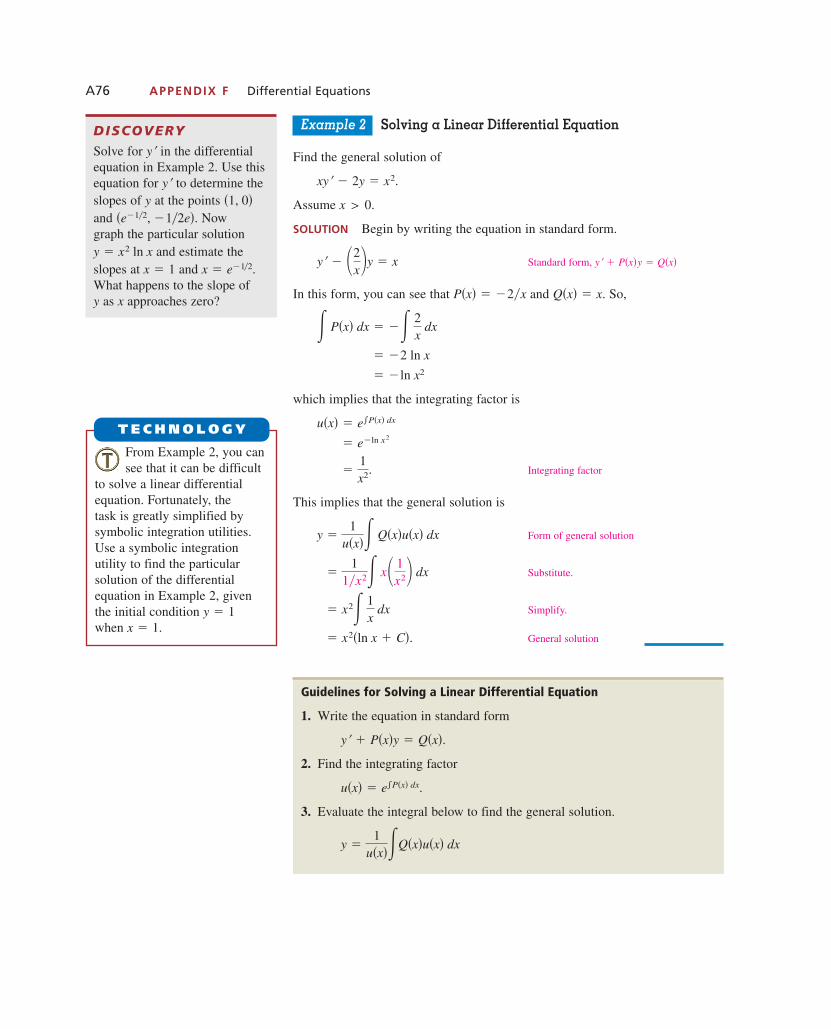
A76 APPENDIX F Differential Equations
Example 2 Solving a Linear Differential Equation
Find the general solution of
Assume
SOLUTION Begin by writing the equation in standard form.
Standard form,
In this form, you can see that and So,
which implies that the integrating factor is
Integrating factor
This implies that the general solution is
Form of general solution
Substitute.
Simplify.
General solution � x2�ln x � C�.
� x2� 1x dx
�1
1�x2� x� 1x2� dx
y �1
u�x�� Q�x�u�x� dx
�1x2.
� e�ln x2
u�x� � e�P�x� dx
� �ln x2
� �2 ln x
� P�x� dx � �� 2x dx
Q�x� � x.P�x� � �2�x
y� � P�x�y � Q�x�y� � �2x�y � x
x > 0.
xy� � 2y � x2.
Guidelines for Solving a Linear Differential Equation
1. Write the equation in standard form
2. Find the integrating factor
3. Evaluate the integral below to find the general solution.
y �1
u�x��Q�x�u�x� dx
u�x� � e�P�x� dx.
y� � P�x�y � Q�x�.
DISCOVERY
Solve for in the differentialequation in Example 2. Use thisequation for to determine theslopes of at the points and Now graph the particular solution
and estimate theslopes at and What happens to the slope of
as approaches zero?xy
x � e�1�2.x � 1y � x2 ln x
�e�1�2, �1�2e�.�1, 0�y
y�
y�
From Example 2, you cansee that it can be difficult
to solve a linear differentialequation. Fortunately, the task is greatly simplified bysymbolic integration utilities.Use a symbolic integration utility to find the particularsolution of the differentialequation in Example 2, giventhe initial condition when x � 1.
y � 1
T E C H N O L O G Y
1053715_App_F03.qxp 11/5/08 1:24 PM Page A76
APPENDIX F.3 First-Order Linear Differential Equation A77
Application
Example 3 Finding a Balance
You are setting up a “continuous annuity” trust fund. For 20 years, money is continuously transferred from your checking account to the trust fund at the rateof $1000 per year (about $2.74 per day). The account earns 8% interest,compounded continuously. What is the balance in the account after 20 years?
SOLUTION Let A represent the balance after t years. The balance increases intwo ways: with interest and with additional deposits. The rate at which the balance is changing can be modeled by
In standard form, this linear differential equation is
Standard form
which implies that and The general solution is
General solution
Because when you can determine that So, the revenueafter 20 years is
� $49,412.91.
�12,500 � 61,912.91
A � �12,500 � 12,500e0.08�20�
C � 12,500.t � 0,A � 0
A � �12,500 � Ce0.08t.
Q�t� � 1000.P�t� � �0.08
dAdt
� 0.08A � 1000
dAdt
� 0.08A � 1000.
1. Given a first-order linear differential equation, what does the term “first-order” refer to?
2. True or false: is a first-order linear differential equation.
3. Give the standard form of a first-order linear differential equation. Whatis its integrating factor?
4. Give the guidelines for solving a first-order linear differential equation.
y� 11x
y � x 1 1
C O N C E P T C H E C K
Interest Deposits
1053715_App_F03.qxp 11/5/08 1:24 PM Page A77

A78 APPENDIX F Differential Equations
In Exercises 1–6, write the linear differential equationin standard form.
1. 2.
3. 4.
5. 6.
In Exercises 7–18, solve the differential equation.
7. 8.
9. 10.
11. 12.
13. 14.
15. 16.
17. 18.
In Exercises 19–22, solve for in two ways.
19. 20.
21. 22.
In Exercises 23–26, match the differential equationwith its solution.
Differential Equation Solution
23. (a)
24. (b)
25. (c)
26. (d)
In Exercises 27–34, find the particular solution that satisfies the initial condition.
Differential Equation Initial Condition
27.
28.
29.
30.
31.
32.
33.
34. y � 10 when x � 1x2y� � 4xy � 10
y � 5 when x � 1xy� � 2y � �x2
y � 2 when x � 1y� � �2x � 1�y � 0
y � 6 when x � 0y� � 3x2y � 3x2
y � 4 when x � 0y� � y � x
y � 2 when x � 2xy� � y � 0
y � 4 when x � 1y� � 2y � e�2x
y � 3 when x � 0y� � y � 6ex
y � Ce2xy� � 2xy � x
y � x2 � Cy� � 2xy � 0
y � �12 � Cex2y� � 2y � 0
y � Cex2y� � 2x � 0
y� � 4xy � xy� � 2xy � 2x
y� � 10y � 5y� � y � 4
y
xy� � y � x2 ln xx3y� � 2y � e1�x2
xy� � y � x2 � 1�x � 1�y� � y � x2 � 1
y� � 5y � e5xy� � 5xy � x
dydx
�2yx
� 3x � 1dydx
�yx
� 3x � 4
dydx
� 3y � e�3xdydx
� y � e�x
dydx
� 5y � 15dydx
� 3y � 6
x � x 2�y� � y�y � 1 � �x � 1�y�
xy� � y � x3yxy� � y � xex
y� � 5�2x � y� � 0x3 � 2x2y� � 3y � 0
The following warm-up exercises involve skills that were covered in earlier sections. You willuse these skills in the exercise set for this section. For additional help, review Sections 10.1,10.4, 11.2, and 11.3.
In Exercises 1–4, simplify the expression.
1. 2.
3. 4.
In Exercises 5–10, find the indefinite integral.
5.
6.
7.
8.
9.
10. � x�1 � x 2�2 dx
� �4x � 3�2 dx
� x � 1
x 2 � 2x � 3 dx
� 1
2x � 5 dx
� xe3x2 dx
� 4e2x dx
e2 ln x�xe�ln x3
1e�x �e�x � e2x�e�x�e2x � ex�
Skills Review F.3
Exercises F.3 See www.CalcChat.com for worked-out solutions to odd-numbered exercises.
1053715_App_F03.qxp 11/5/08 1:24 PM Page A78
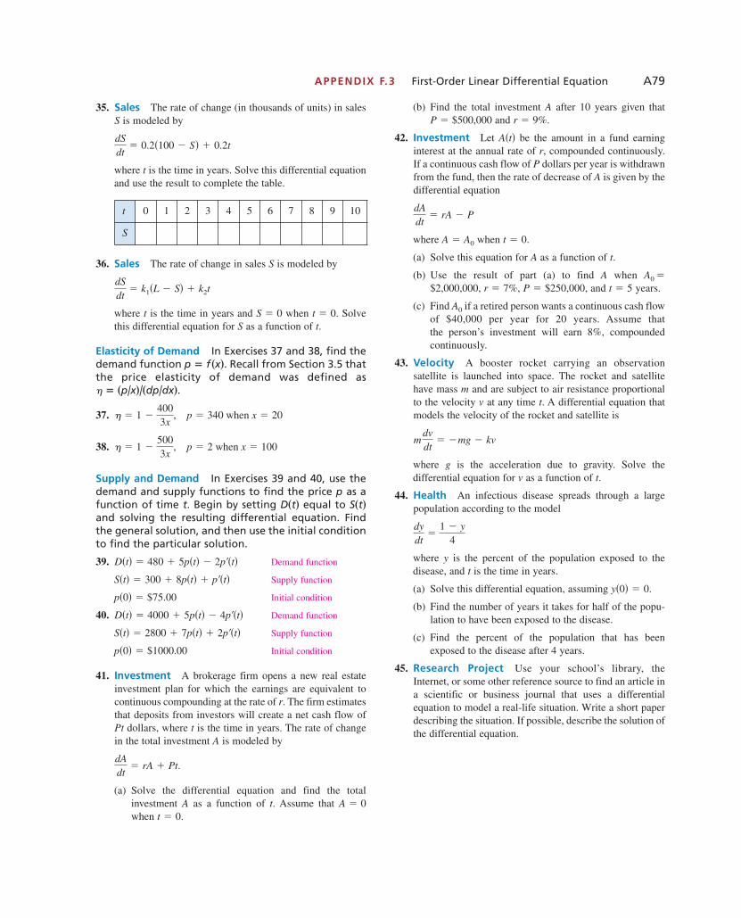
APPENDIX F.3 First-Order Linear Differential Equation A79
35. Sales The rate of change (in thousands of units) in salesis modeled by
where is the time in years. Solve this differential equationand use the result to complete the table.
36. Sales The rate of change in sales is modeled by
where is the time in years and when Solvethis differential equation for as a function of
Elasticity of Demand In Exercises 37 and 38, find thedemand function Recall from Section 3.5 thatthe price elasticity of demand was defined as
37.
38.
Supply and Demand In Exercises 39 and 40, use thedemand and supply functions to find the price as afunction of time Begin by setting equal to and solving the resulting differential equation. Findthe general solution, and then use the initial conditionto find the particular solution.
39. Demand function
Supply function
Initial condition
40. Demand function
Supply function
Initial condition
41. Investment A brokerage firm opens a new real estateinvestment plan for which the earnings are equivalent tocontinuous compounding at the rate of The firm estimatesthat deposits from investors will create a net cash flow of
dollars, where is the time in years. The rate of changein the total investment is modeled by
(a) Solve the differential equation and find the total investment as a function of Assume that when
(b) Find the total investment A after 10 years given thatand
42. Investment Let be the amount in a fund earninginterest at the annual rate of compounded continuously.If a continuous cash flow of dollars per year is withdrawnfrom the fund, then the rate of decrease of is given by thedifferential equation
where when
(a) Solve this equation for as a function of
(b) Use the result of part (a) to find when and years.
(c) Find if a retired person wants a continuous cash flowof $40,000 per year for 20 years. Assume that the person’s investment will earn 8%, compounded continuously.
43. Velocity A booster rocket carrying an observation satellite is launched into space. The rocket and satellitehave mass and are subject to air resistance proportionalto the velocity at any time A differential equation thatmodels the velocity of the rocket and satellite is
where is the acceleration due to gravity. Solve the differential equation for as a function of
44. Health An infectious disease spreads through a largepopulation according to the model
where is the percent of the population exposed to the disease, and is the time in years.
(a) Solve this differential equation, assuming
(b) Find the number of years it takes for half of the popu-lation to have been exposed to the disease.
(c) Find the percent of the population that has beenexposed to the disease after 4 years.
45. Research Project Use your school’s library, theInternet, or some other reference source to find an article ina scientific or business journal that uses a differentialequation to model a real-life situation. Write a short paperdescribing the situation. If possible, describe the solution ofthe differential equation.
y�0� � 0.
ty
dydt
�1 � y
4
t.vg
mdvdt
� �mg � kv
t.vm
A0
t � 5P � $250,000,r � 7%,$2,000,000,A0 �A
t.A
t � 0.A � A0
dAdt
� rA � P
AP
r,A�t�
r � 9%.P � $500,000
t � 0.A � 0t.A
dAdt
� rA � Pt.
AtPt
r.
p�0� � $1000.00
S�t� � 2800 � 7p�t� � 2p��t�D�t� � 4000 � 5p�t� � 4p��t�p�0� � $75.00
S�t� � 300 � 8p�t� � p��t�D�t� � 480 � 5p�t� � 2p��t�
St�Dt�t.p
p � 2 when x � 100� � 1 �5003x
,
p � 340 when x � 20� � 1 �4003x
,
� � p/x�/dp/dx�.
p � f x�.
t.St � 0.S � 0t
dSdt
� k1�L � S� � k2t
S
t
dSdt
� 0.2�100 � S� � 0.2t
S
t 0 1 2 3 4 5 6 7 8 9 10
S
1053715_App_F03.qxp 11/5/08 1:24 PM Page A79

A80 APPENDIX F Differential Equations
F.4 Applications of Differential EquationsUse differential equations to model and solve real-life problems.
Example 1 Modeling Advertising Awareness
The new cereal product from Example 3 in Section F.1 is introduced through anadvertising campaign to a population of 1 million potential customers. The rate atwhich the population hears about the product is assumed to be proportional to thenumber of people who are not yet aware of the product. By the end of 1 year, halfof the population has heard of the product. How many will have heard of it by theend of 2 years?
SOLUTION Let y be the number (in millions) of people at time t who have heardof the product. This means that is the number of people who have notheard of it, and is the rate at which the population hears about the product.From the given assumption, you can write the differential equation as shown.
Using separation of variables or a symbolic integration utility, you can find thegeneral solution to be
General solution
To solve for the constants C and k, use the initial conditions. That is, becausewhen you can determine that Similarly, because
when it follows that which implies that
So, the particular solution is
Particular solution
This model is shown graphically in Figure F.7. Using the model, you can deter-mine that the number of people who have heard of the product after 2 years is
� 0.75 or 750,000 people.
y � 1 � e�0.693�2�
y � 1 � e�0.693t.
k � ln 2 � 0.693.
0.5 � 1 � e�k,t � 1,y � 0.5C � 1.t � 0,y � 0
y � 1 � Ce�kt.
dydt
� k�1 � y�
dy�dt�1 � y�
Rate ofchange
of y
is propor-tional to
y
t
1.25
1.00
0.75
0.50
0.25
y = 1 − e−0.693t
(2, 0.75)
(1, 0.50)
(0, 0)
1 2 3 4 5
Time (in years)
Pote
ntia
l cus
tom
ers
(in
mill
ions
)
Advertising Awareness
FIGURE F.7
the differencebetween 1
and y.
1053715_App_F04.qxp 11/5/08 1:25 PM Page A80
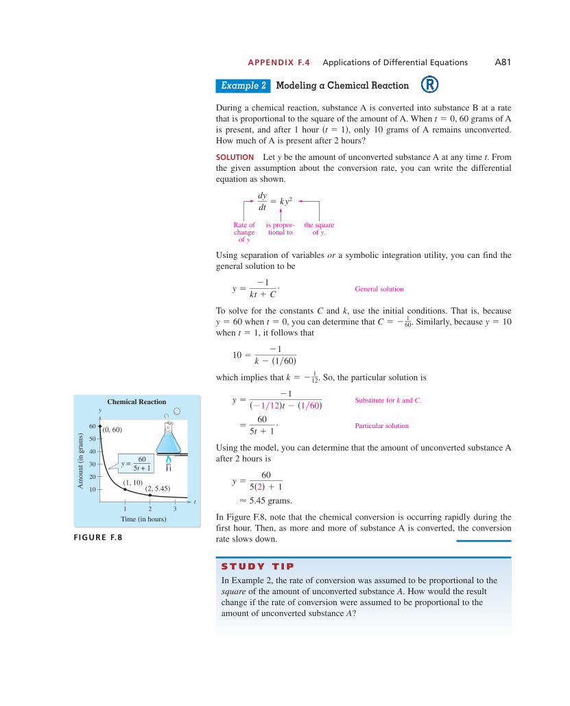
APPENDIX F.4 Applications of Differential Equations A81
Example 2 Modeling a Chemical Reaction
During a chemical reaction, substance A is converted into substance B at a ratethat is proportional to the square of the amount of A. When 60 grams of Ais present, and after 1 hour only 10 grams of A remains unconverted.How much of A is present after 2 hours?
SOLUTION Let y be the amount of unconverted substance A at any time t. Fromthe given assumption about the conversion rate, you can write the differentialequation as shown.
Using separation of variables or a symbolic integration utility, you can find thegeneral solution to be
General solution
To solve for the constants C and k, use the initial conditions. That is, becausewhen you can determine that Similarly, because
when it follows that
which implies that So, the particular solution is
Substitute for k and C.
Particular solution
Using the model, you can determine that the amount of unconverted substance Aafter 2 hours is
In Figure F.8, note that the chemical conversion is occurring rapidly during thefirst hour. Then, as more and more of substance A is converted, the conversionrate slows down.
� 5.45 grams.
y �60
5�2� � 1
�60
5t � 1.
y ��1
��1�12�t � �1�60�
k � �112.
10 ��1
k � �1�60�
t � 1,y � 10C � �
160.t � 0,y � 60
y ��1
kt � C.
dydt
� ky2
�t � 1�,t � 0,
Rate ofchange
of y
is propor-tional to
the squareof y.
S T U D Y T I PIn Example 2, the rate of conversion was assumed to be proportional to thesquare of the amount of unconverted substance How would the resultchange if the rate of conversion were assumed to be proportional to theamount of unconverted substance A?
A.
y
t
60
50
40
30
20
10
(0, 60)
(1, 10)(2, 5.45)
y = 605t + 1
1 2 3
Time (in hours)
Am
ount
(in
gra
ms)
Chemical Reaction
FIGURE F.8
1053715_App_F04.qxp 11/5/08 1:25 PM Page A81

A82 APPENDIX F Differential Equations
Earlier in the text, you studied two models for population growth:exponential growth, which assumes that the rate of change of y is proportional toy, and logistic growth, which assumes that the rate of change of y is proportionalto y and where L is the population limit.
The next example describes a third type of growth model called a Gompertzgrowth model. This model assumes that the rate of change of y is proportional toy and the natural log of where L is the population limit.
Example 3 Modeling Population Growth
A population of 20 wolves has been introduced into a national park. The forestservice estimates that the maximum population the park can sustain is 200wolves. After 3 years, the population is estimated to be 40 wolves. If thepopulation follows a Gompertz growth model, how many wolves will there be 10 years after their introduction?
SOLUTION Let y be the number of wolves at any time t. From the givenassumption about the rate of growth of the population, you can write the differential equation as shown.
Using separation of variables or a symbolic integration utility, you can find thegeneral solution to be
General solution
To solve for the constants C and k, use the initial conditions. That is, becausewhen you can determine that
Similarly, because when it follows that
which implies that So, the particular solution is
Particular solution
Using the model, you can estimate the wolf population after 10 years to be
In Figure F.9, note that after 10 years the population has reached about half of theestimated maximum population. Try checking the growth model to see that ityields when and when t � 3.y � 40t � 0y � 20
� 100 wolves.
y � 200e�2.3026e�0.1194�10�
y � 200e�2.3026e�0.1194t.
k � 0.1194.
40 � 200e�2.3026e�3k
t � 3,y � 40
� 2.3026.
C � ln 10
t � 0,y � 20
y � 200e�Ce�kt.
dydt
� ky ln 200
y
L�y,
1 � y�L,
Rate ofchange
of y
is propor-tional to
the productof y and
the log ofthe ratio of200 and y.
y
t
20018016014012010080604020 (0, 20)
(3, 40)
(10, 100)
y = 200e−2.3026e−0.1194t
Num
ber
of w
olve
s
2 4 6 8 10 12 14
Time (in years)
Population Growth
FIGURE F.9
1053715_App_F04.qxp 11/5/08 1:25 PM Page A82
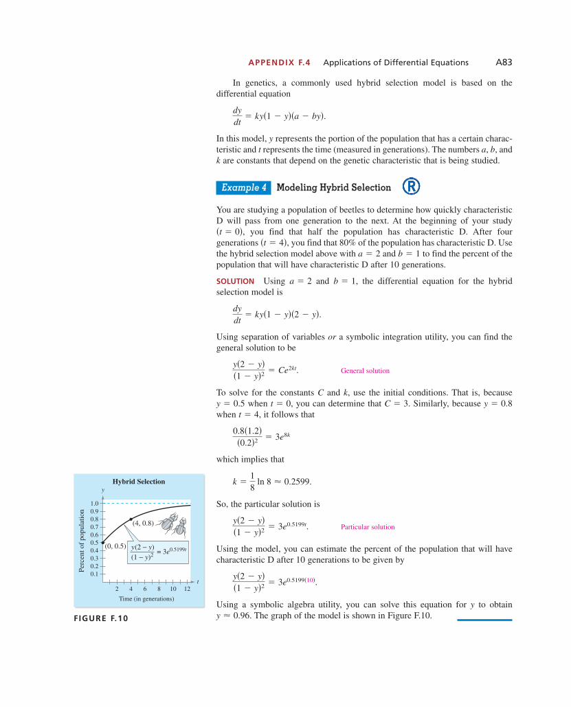
APPENDIX F.4 Applications of Differential Equations A83
In genetics, a commonly used hybrid selection model is based on the differential equation
In this model, y represents the portion of the population that has a certain charac-teristic and t represents the time (measured in generations). The numbers a, b, andk are constants that depend on the genetic characteristic that is being studied.
Example 4 Modeling Hybrid Selection
You are studying a population of beetles to determine how quickly characteristicD will pass from one generation to the next. At the beginning of your study
you find that half the population has characteristic D. After fourgenerations you find that 80% of the population has characteristic D. Usethe hybrid selection model above with and to find the percent of thepopulation that will have characteristic D after 10 generations.
SOLUTION Using and the differential equation for the hybridselection model is
Using separation of variables or a symbolic integration utility, you can find thegeneral solution to be
General solution
To solve for the constants C and k, use the initial conditions. That is, becausewhen you can determine that Similarly, because
when it follows that
which implies that
So, the particular solution is
Particular solution
Using the model, you can estimate the percent of the population that will havecharacteristic D after 10 generations to be given by
Using a symbolic algebra utility, you can solve this equation for y to obtainThe graph of the model is shown in Figure F.10.y � 0.96.
y�2 � y��1 � y�2 � 3e0.5199�10�.
y�2 � y��1 � y�2 � 3e0.5199t.
k �18
ln 8 � 0.2599.
0.8�1.2��0.2�2 � 3e8k
t � 4,y � 0.8C � 3.t � 0,y � 0.5
y�2 � y��1 � y�2 � Ce2kt.
dydt
� ky�1 � y��2 � y�.
b � 1,a � 2
b � 1a � 2�t � 4�,
�t � 0�,
dydt
� ky�1 � y��a � by�.
y
t
1.00.90.80.70.60.50.40.30.20.1
(0, 0.5)
(4, 0.8)
Perc
ent o
f po
pula
tion
2 4 6 8 10 12
Time (in generations)
Hybrid Selection
y(2 − y)(1 − y)2 = 3e0.5199t
FIGURE F.10
1053715_App_F04.qxp 11/5/08 1:25 PM Page A83

A84 APPENDIX F Differential Equations
Example 5 Modeling a Chemical Mixture
A tank contains 40 gallons of a solution composed of 90% water and 10% alcohol.A second solution containing half water and half alcohol is added to the tank at the rate of 4 gallons per minute. At the same time, the tank is being drained at therate of 4 gallons per minute, as shown in Figure F.11. Assuming that the solution isstirred constantly, how much alcohol will be in the tank after 10 minutes?
SOLUTION Let y be the number of gallons of alcohol in the tank at any time t.The percent of alcohol in the 40-gallon tank at any time is Moreover,because 4 gallons of solution is being drained each minute, the rate of change ofy is
where 2 represents the number of gallons of alcohol entering each minute in the50% solution. In standard form, this linear differential equation is
Standard form
Using an integrating factor or a symbolic integration utility, you can find the gen-eral solution to be
General solution
Because when you can conclude that So, the particularsolution is
Particular solution
Using this model, you can determine that the amount of alcohol in the tank whenis
� 14.1 gallons.
y � 20 � 16e��10��10
t � 10
y � 20 � 16e�t�10.
C � �16.t � 0,y � 4
y � 20 � Ce�t�10.
y� �110
y � 2.
dydt
� �4� y40� � 2
y�40.
4 gal/min
4 gal/min
FIGURE F.11
1. What does the exponential growth model assume about the rate ofchange of
2. What does the logistic growth model assume about the rate of change of
3. What does the Gompertz growth model assume about the rate of changeof
4. In the logistic and Gompertz growth models, what does represent?L
y?
y?
y?
C O N C E P T C H E C K
Rate ofchange
of y
is equal to theamount of alcohol
draining out
plus the amountof alcoholentering.
1053715_App_F04.qxp 11/5/08 1:25 PM Page A84
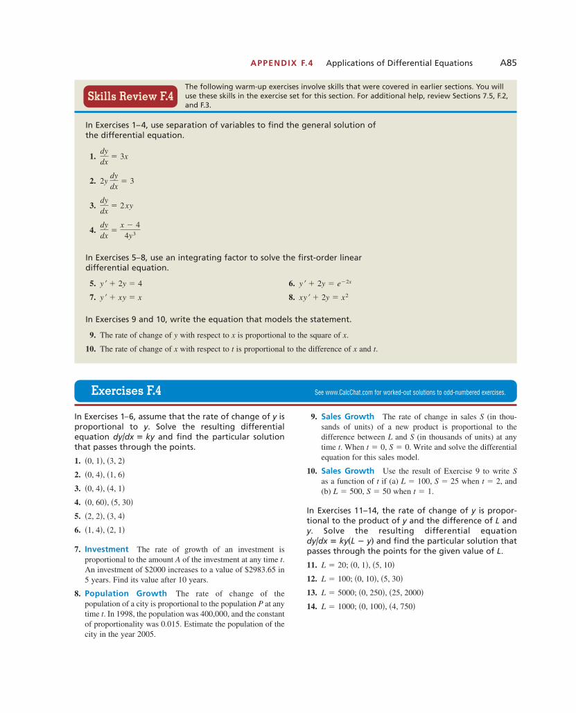
APPENDIX F.4 Applications of Differential Equations A85
In Exercises 1–6, assume that the rate of change of isproportional to Solve the resulting differentialequation and find the particular solutionthat passes through the points.
1.
2.
3.
4.
5.
6.
7. Investment The rate of growth of an investment isproportional to the amount of the investment at any time An investment of $2000 increases to a value of $2983.65 in 5 years. Find its value after 10 years.
8. Population Growth The rate of change of thepopulation of a city is proportional to the population at anytime In 1998, the population was 400,000, and the constantof proportionality was 0.015. Estimate the population of thecity in the year 2005.
9. Sales Growth The rate of change in sales (in thou-sands of units) of a new product is proportional to the difference between and (in thousands of units) at anytime When Write and solve the differentialequation for this sales model.
10. Sales Growth Use the result of Exercise 9 to write as a function of if (a) when and (b) when
In Exercises 11–14, the rate of change of is propor-tional to the product of and the difference of and
Solve the resulting differential equationand find the particular solution that
passes through the points for the given value of
11.
12.
13.
14. L � 1000; �0, 100�, �4, 750�L � 5000; �0, 250�, �25, 2000�L � 100; �0, 10�, �5, 30�L � 20; �0, 1�, �5, 10�
L.dy/dx � ky�L � yy.
Lyy
t � 1.S � 50L � 500,t � 2,S � 25L � 100,t
S
S � 0.t � 0,t.SL
S
t.P
t.A
�1, 4�, �2, 1��2, 2�, �3, 4��0, 60�, �5, 30��0, 4�, �4, 1��0, 4�, �1, 6��0, 1�, �3, 2�
dy/dx � kyy.
y
The following warm-up exercises involve skills that were covered in earlier sections. You willuse these skills in the exercise set for this section. For additional help, review Sections 7.5, F.2,and F.3.
In Exercises 1–4, use separation of variables to find the general solution ofthe differential equation.
1.
2.
3.
4.
In Exercises 5–8, use an integrating factor to solve the first-order linear differential equation.
5. 6.
7. 8.
In Exercises 9 and 10, write the equation that models the statement.
9. The rate of change of with respect to is proportional to the square of
10. The rate of change of with respect to is proportional to the difference of and t.xtx
x.xy
xy� � 2y � x2y� � xy � x
y� � 2y � e�2xy� � 2y � 4
dydx
�x � 4
4y3
dydx
� 2xy
2y dydx
� 3
dydx
� 3x
Skills Review F.4
Exercises F.4 See www.CalcChat.com for worked-out solutions to odd-numbered exercises.
1053715_App_F04.qxp 11/5/08 1:25 PM Page A85

A86 APPENDIX F Differential Equations
15. Biology At any time the rate of growth of the popula-tion of deer in a state park is proportional to the productof and where is the maximum numberof deer the park can maintain. When andwhen Write as a function of
16. Sales Growth The rate of change in sales (inthousands of units) of a new product is proportional to the product of and (in thousands of units) is the estimated maximum level of sales, and when Write and solve the differential equation for this salesmodel.
Learning Theory In Exercises 17 and 18, assume thatthe rate of change in the proportion of correctresponses after trials is proportional to the productof and where is the limiting proportion ofcorrect responses.
17. Write and solve the differential equation for this learningtheory model.
18. Use the solution of Exercise 17 to write as a function ofand then use a graphing utility to graph the solution.
(a) (b)
when when
when when
Chemical Reaction In Exercises 19 and 20, use thechemical reaction model in Example 2 to find theamount as a function of and use a graphing utilityto graph the function.
19. grams when grams when
20. grams when grams when
In Exercises 21 and 22, use the Gompertz growthmodel described in Example 3 to find the growth function, and sketch its graph.
21. when when
22. when when
23. Biology A population of eight beavers has beenintroduced into a new wetlands area. Biologists estimatethat the maximum population the wetlands can sustain is 60beavers. After 3 years, the population is 15 beavers. If thepopulation follows a Gompertz growth model, how manybeavers will be in the wetlands after 10 years?
24. Biology A population of 30 rabbits has been introducedinto a new region. It is estimated that the maximumpopulation the region can sustain is 400 rabbits. After 1 year, the population is estimated to be 90 rabbits. If thepopulation follows a Gompertz growth model, how manyrabbits will be present after 3 years?
Biology In Exercises 25 and 26, use the hybridselection model in Example 4 to find the percent ofthe population that has the indicated characteristic.
25. You are studying a population of mayflies to determine howquickly characteristic A will pass from one generation to thenext. At the start of the study, half the population has charac-teristic A. After four generations, 75% of the population hascharacteristic A. Find the percent of the population that willhave characteristic A after 10 generations. (Assume and )
26. A research team is studying a population of snails to determine how quickly characteristic B will pass from onegeneration to the next. At the start of the study, 40% of thesnails have characteristic B. After five generations, 80% ofthe population has characteristic B. Find the percent of the population that will have characteristic B after eightgenerations. (Assume and )
27. Chemical Reaction In a chemical reaction, a compoundchanges into another compound at a rate proportional to theunchanged amount, according to the model
(a) Solve the differential equation.
(b) If the initial amount of the original compound is 20 grams, and the amount remaining after 1 hour is 16 grams, when will 75% of the compound have beenchanged?
28. Chemical Mixture A 100-gallon tank is full of a solution containing 25 pounds of a concentrate. Starting attime distilled water is admitted to the tank at the rate of 5 gallons per minute, and the well-stirred solution iswithdrawn at the same rate.
(a) Find the amount Q of the concentrate in the solution asa function of (Hint: )
(b) Find the time when the amount of concentrate in thetank reaches 15 pounds.
29. Chemical Mixture A 200-gallon tank is half full ofdistilled water. At time a solution containing 0.5pound of concentrate per gallon enters the tank at the rateof 5 gallons per minute, and the well-stirred mixture iswithdrawn at the same rate. Find the amount Q ofconcentrate in the tank after 30 minutes. Hint:
30. Safety Assume that the rate of change per hour in thenumber of miles of road cleared by a snowplow isinversely proportional to the depth of snow. That is,
Find as a function of if miles when inchesand miles when inches �2 ≤ h ≤ 15�.h � 6s � 12
h � 2s � 25hs
dsdh
�kh
.
hs
Q� � Q�20 �52�
�
t � 0,
Q� � Q�20 � 0t.
t � 0,
dydt
� ky.
b � 1.a � 2
b � 1.a � 2
t � 1t � 0; y � 625L � 5000; y � 500
t � 2t � 0; y � 150L � 500; y � 100
t � 1y � 12t � 0;y � 75
t � 2y � 4t � 0;y � 45
t,y
n � 10P � 0.60n � 4P � 0.85
n � 0P � 0.25n � 0P � 0.50
L � 0.80L � 1.00
n,P
LL � P,Pn
P
t � 0.S � 10LL � S.S
S
t.NN � 200.t � 4,N � 100,t � 0,
L � 500L � N,NN
t,
1053715_App_F04.qxp 11/5/08 1:25 PM Page A86

APPENDIX F.4 Applications of Differential Equations A87
31. Chemistry A wet towel hung from a clothesline to dryloses moisture through evaporation at a rate proportional toits moisture content. If after 1 hour the towel has lost 40%of its original moisture content, after how long will it havelost 80%?
32. Biology Let and be the sizes of two internal organsof a particular mammal at time Empirical data indicatethat the relative growth rates of these two organs are equal,and can be modeled by
Use this differential equation to write as a function of
33. Population Growth When predicting populationgrowth, demographers must consider birth and death ratesas well as the net change caused by the difference betweenthe rates of immigration and emigration. Let be thepopulation at time and let be the net increase per unittime due to the difference between immigration and emi-gration. So, the rate of growth of the population is given by
is constant.
Solve this differential equation to find as a function oftime.
34. Meteorology The barometric pressure (in inches ofmercury) at an altitude of miles above sea level decreasesat a rate proportional to the current pressure according tothe model
where inches when Find the barometricpressure (a) at the top of Mt. St. Helens (8364 feet) and (b) at the top of Mt. McKinley (20,320 feet).
35. Investment A large corporation starts at time toinvest part of its receipts at a rate of dollars per year in afund for future corporate expansion. Assume that the fundearns percent interest per year compounded continuously.So, the rate of growth of the amount in the fund is givenby
where when Solve this differential equationfor as a function of
Investment In Exercises 36–38, use the result ofExercise 35.
36. Find for each situation.
(a)
(b)
37. Find if the corporation needs $120,000,000 in 8 years andthe fund earns interest compounded continuously.
38. Find if the corporation needs $800,000 and it can invest$75,000 per year in a fund earning 13% interestcompounded continuously.
Medical Science In Exercises 39–41, a medicalresearcher wants to determine the concentration (inmoles per liter) of a tracer drug injected into a movingfluid. Solve this problem by considering a single-compartment dilution model (see figure). Assume thatthe fluid is continuously mixed and that the volume offluid in the compartment is constant.
Figure for 39– 41
39. If the tracer is injected instantaneously at time thenthe concentration of the fluid in the compartment beginsdiluting according to the differential equation
(a) Solve this differential equation to find the concentra-tion as a function of time.
(b) Find the limit of as
40. Use the solution of the differential equation in Exercise 39to find the concentration as a function of time, and use agraphing utility to graph the function.
(a)
(b)
41. In Exercises 39 and 40, it was assumed that there was a single initial injection of the tracer drug into the compartment. Now consider the case in which the tracer iscontinuously injected (beginning at ) at the rate of mol/min. Considering to be negligible compared with use the differential equation
(a) Solve this differential equation to find the concentra-tion as a function of time.
(b) Find the limit of as t →�.C
C � 0 when t � 0.dCdt
�QV
� �RV�C,
R,QQt � 0
V � 2 liters, R � 1.5 L�min, and C0 � 0.6 mol�L
V � 2 liters, R � 0.5 L�min, and C0 � 0.6 mol�L
t →�.C
C � C0 when t � 0.dCdt
� ��RV�C,
t � 0,
Flow R (pure)
Flow R(concentration C)
Volume V
Tracerinjected
C
t
1614 %
P
P � $250,000, r � 15%, and t � 10 years
P � $100,000, r � 12%, and t � 5 years
A
t.At � 0.A � 0
dAdt
� rA � P
Ar
Pt � 0
x � 0.y � 29.92
dydx
� �0.2y
xy
P
NdPdt
� kP � N,
NtP
x.y
1x dxdt
�1y dydt
.
t.yx
1053715_App_F04.qxp 11/5/08 1:25 PM Page A87
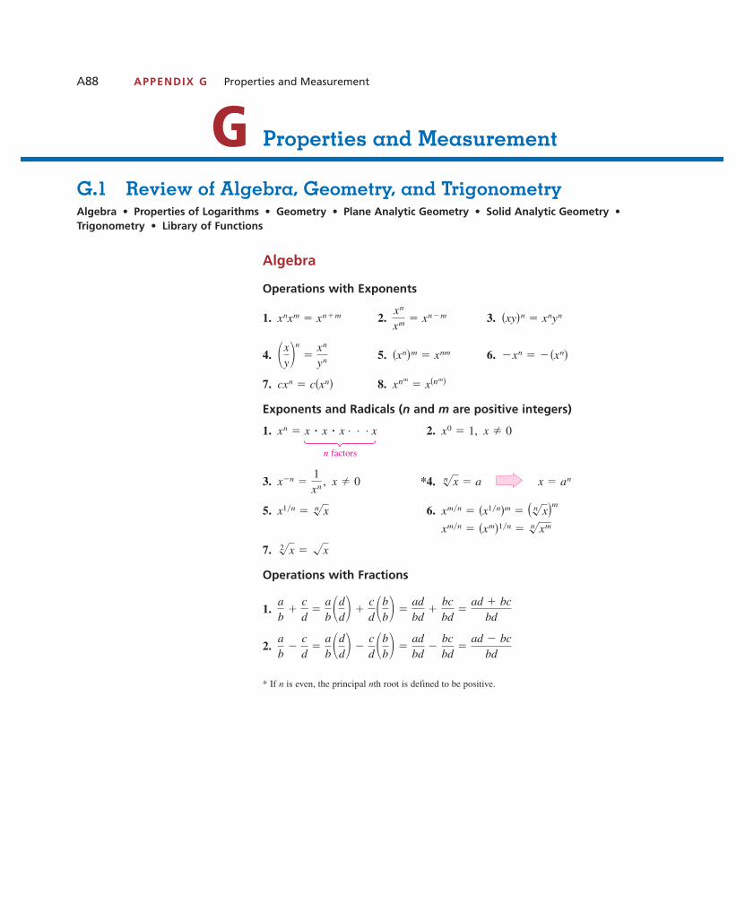
A88 APPENDIX G Properties and Measurement
G.1 Review of Algebra, Geometry, and TrigonometryAlgebra • Properties of Logarithms • Geometry • Plane Analytic Geometry • Solid Analytic Geometry •Trigonometry • Library of Functions
G Properties and Measurement
Algebra
Operations with Exponents
1. 2. 3.
4. 5. 6.
7. 8.
Exponents and Radicals (n and m are positive integers)
1. 2.
n factors
3. *4.
5. 6.
7.
Operations with Fractions
1.
2.
* If n is even, the principal nth root is defined to be positive.
ab
�cd
�ab �
dd� �
cd �
bb� �
adbd
�bcbd
�ad � bc
bd
ab
�cd
�ab �
dd� �
cd �
bb� �
adbd
�bcbd
�ad � bc
bd
2�x � �x
xm�n � �xm�1�n � n�xm
xm�n � �x1�n�m � � n�x�mx1�n � n�x
x � ann�x � ax � 0x�n �1xn ,
x � 0x0 � 1,xn � x � x � x . . . x
xnm� x�nm�cxn � c�xn�
�xn � ��xn��xn�m � xnm�xy�
n
�xn
yn
�xy�n � xnynxn
xm � xn�mxnxm � xn�m
1053715_App_G.1.qxp 11/5/08 1:27 PM Page A88

APPENDIX G.1 Review of Algebra, Geometry, and Trigonometry A89
3.
4.
5.
Quadratic Formula
Factors and Special Products
1.
2.
3.
4.
Factoring by Grouping
Binomial Theorem
1.
2.
3.
4.
5.
6.
7.
. . . � nan�1x � an
�x � a�n � xn � naxn�1 �n�n � 1�
2!a2xn�2 �
n�n � 1��n � 2�3!
a3xn�3 �
�x � a�4 � x4 � 4ax3 � 6a2x2 � 4a3x � a4
�x � a�4 � x4 � 4ax3 � 6a2x2 � 4a3x � a4
�x � a�3 � x3 � 3ax2 � 3a2x � a3
�x � a�3 � x3 � 3ax2 � 3a2x � a3
�x � a�2 � x2 � 2ax � a2
�x � a�2 � x2 � 2ax � a2
acx3 � adx2 � bcx � bd � ax2�cx � d� � b�cx � d� � �ax2 � b��cx � d�
x4 � a4 � �x � a��x � a��x2 � a2�
x3 � a3 � �x � a��x2 � ax � a2�
x3 � a3 � �x � a��x2 � ax � a2�
x2 � a2 � �x � a��x � a�
x ��b ± �b2 � 4ac
2aax2 � bx � c � 0
ab � acad
�a�b � c�
ad�
b � cd
abac
�bc
a�bc
�a�bc�1
� �ab��
1c� �
abc
a�bc�d
� �ab��
dc� �
adbc
�ab��
cd� �
acbd
1053715_App_G.1.qxp 11/5/08 1:27 PM Page A89
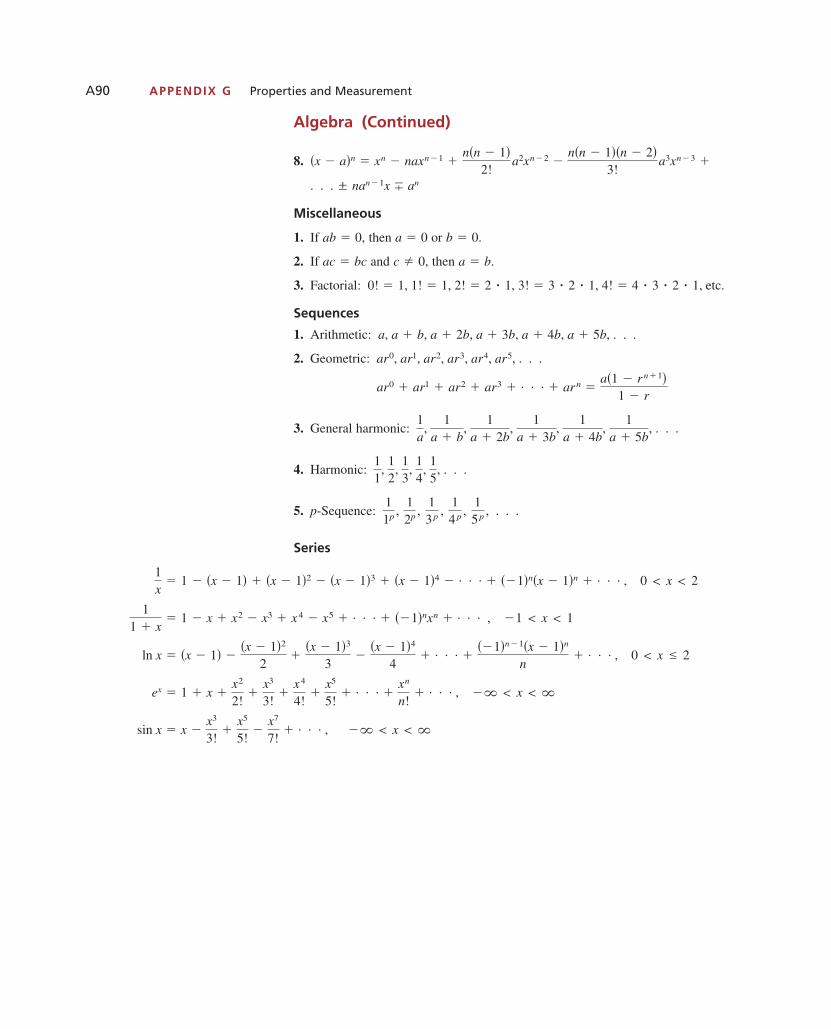
A90 APPENDIX G Properties and Measurement
Algebra (Continued)
8.
Miscellaneous
1. If then or
2. If and then
3. Factorial: etc.
Sequences
1. Arithmetic:
2. Geometric:
3. General harmonic:
4. Harmonic:
5. p-Sequence:
Series
11p ,
12p ,
13p ,
14p ,
15p , . . .
11
, 12
, 13
, 14
, 15
, . . .
1a
, 1
a � b,
1a � 2b
, 1
a � 3b,
1a � 4b
, 1
a � 5b, . . .
ar0 � ar1 � ar2 � ar3 � . . . � arn �a�1 � rn�1�
1 � r
ar0, ar1, ar2, ar3, ar4, ar5, . . .
a, a � b, a � 2b, a � 3b, a � 4b, a � 5b, . . .
0! � 1, 1! � 1, 2! � 2 � 1, 3! � 3 � 2 � 1, 4! � 4 � 3 � 2 � 1,
a � b.c � 0,ac � bc
b � 0.a � 0ab � 0,
. . . ± nan�1x � an
�x � a�n � xn � naxn�1 �n�n � 1�
2!a2xn�2 �
n�n � 1��n � 2�3!
a3xn�3 �
�� < x < � sin x � x �x3
3!�
x5
5!�
x7
7!� . . . ,
�� < x < � ex � 1 � x �x2
2!�
x3
3!�
x4
4!�
x5
5!� . . . �
xn
n!� . . . ,
0 < x 2 ln x � �x � 1� ��x � 1�2
2�
�x � 1�3
3�
�x � 1�4
4� . . . �
��1�n�1�x � 1�n
n� . . . ,
�1 < x < 1 1
1 � x� 1 � x � x2 � x3 � x4 � x5 � . . . � ��1�nxn � . . . ,
0 < x < 2 1x
� 1 � �x � 1� � �x � 1�2 � �x � 1�3 � �x � 1�4 � . . . � ��1�n�x � 1�n � . . . ,
1053715_App_G.1.qxp 11/5/08 1:27 PM Page A90

APPENDIX G.1 Review of Algebra, Geometry, and Trigonometry A91
Properties of Logarithms
Inverse Properties
1. 2.
Properties of Logarithms
1. 2.
3. 4.
5. 6.
Geometry
Triangles
1. General triangle
Sum of triangles
Area (base)(height)
2. Similar triangles
3. Right triangle
(Pythagorean Theorem)
Sum of acute angles � � � 90�
c2 � a2 � b2
ab
�AB
�12
bh�12
� � � � 180�
logax �ln xln a
ln xy � y ln x
ln xy
� ln x � ln yln xy � ln x � ln y
ln e � 1ln 1 � 0
eln x � xln ex � x
*
*�1 < x < 1 �1 � x��k � 1 � kx �k�k � 1�x2
2!�
k�k � 1��k � 2�x3
3!�
k�k � 1��k � 2��k � 3�x4
4!� . . . ,
�1 < x < 1 �1 � x�k � 1 � kx �k�k � 1�x2
2!�
k�k � 1��k � 2�x3
3!�
k�k � 1��k � 2��k � 3�x4
4!� . . . ,
�� < x < � cos x � 1 �x2
2!�
x4
4!�
x6
6!� . . . ,
β
α θh
b
b
aβ
α
b
ac
β
α
B
Aβ
α
*The convergence at depends on the value of k.x � ±1
1053715_App_G.1.qxp 11/5/08 1:27 PM Page A91

A92 APPENDIX G Properties and Measurement
Geometry (Continued)
4. Equilateral triangle
Height
Area
5. Isosceles right triangle
Area
Quadrilaterals (Four-Sided Figures)
1. Rectangle 2. Square
Area Area
3. Parallelogram 4. Trapezoid
Area Area
h
a
bh
b
a
h
b
�12
h�a � b�� bh
s
s
w
� �side�2 � s2� �length��width� � lw
�s2
2
��3s2
4
� h ��3s
2
s
s
45°
45°
60°
60° 60°
hs s
s
1053715_App_G.1.qxp 11/5/08 1:27 PM Page A92

APPENDIX G.1 Review of Algebra, Geometry, and Trigonometry A93
Circles and Ellipses
1. Circle 2. Sector of circle in radians
Area Area
Circumference
3. Circular ring 4. Ellipse
Area Area
Circumference
Solid Figures
1. Cone area of base
Volume
2. Right circular cone
Volume
Lateral surface area
3. Frustum of right circular cone
Volume
Lateral surface area � �s�R � r�
�� �r2 � rR � R2�h
3h
r
R
s
� �r�r2 � h2
��r2h
3
h
r
�Ah3
h
A
��A �
b
a
� 2��a2 � b2
2r
R
� �ab� � �R2 � r2�
r
s
θr
s � r � 2�r
� r2
2� �r2
��
1053715_App_G.1.qxp 11/5/08 1:27 PM Page A93

A94 APPENDIX G Properties and Measurement
Geometry (Continued)
4. Right circular cylinder
Volume
Lateral surface area
5. Sphere
Volume
Surface area
Plane Analytic Geometry
Distance Between and
Midpoint Between and
Midpoint
Slope of Line Passing Through and
Slopes of Parallel Lines
Slopes of Perpendicular Lines
Equations of Lines
Point-slope form: General form:
Vertical line: Horizontal line: y � bx � a
Ax � By � C � 0y � y1 � m�x � x1�
m1 � �1
m2
m1 � m2
m �y2 � y1
x2 � x1
�x2, y2��x1, y1�
� �x1 � x2
2,
y1 � y2
2 ��x2, y2��x1, y1�
d � ��x2 � x1�2 � �y2 � y1�2
�x2, y2��x1, y1�
� 4�r2
�43
�r3 r
� 2�rh
� �r2hh
r
1053715_App_G.1.qxp 11/5/08 1:27 PM Page A94
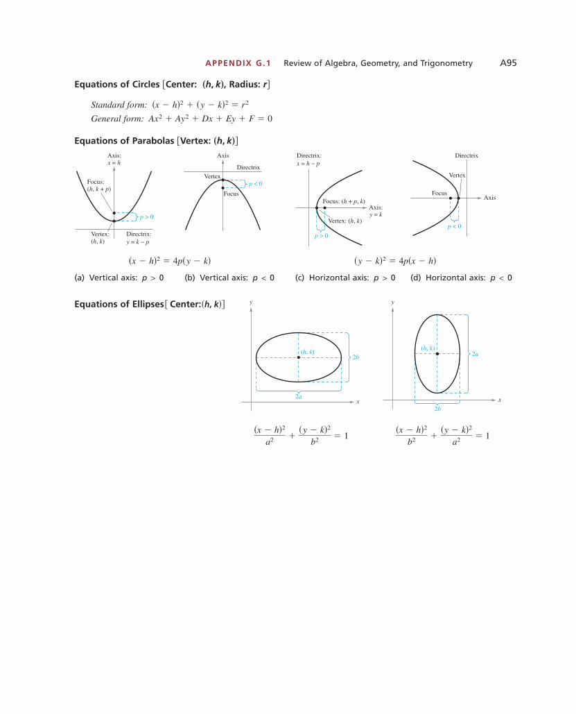
APPENDIX G.1 Review of Algebra, Geometry, and Trigonometry A95
Equations of Parabolas Vertex: h, k
(a) Vertical axis: (b) Vertical axis: (c) Horizontal axis: (d) Horizontal axis:
Equations of Ellipses Center:
�x � h�2
b2 ��y � k�2
a2 � 1�x � h�2
a2 ��y � k�2
b2 � 1
x
(h, k) 2a
2b
y
x
(h, k) 2b
2a
y�h, k�
p < 0p > 0p < 0p > 0
�y � k�2 � 4p�x � h��x � h�2 � 4p�y � k�
p < 0
AxisFocus
Vertex
Directrix
p > 0
Axis:y = k
Focus: (h + p, k)
Vertex: (h, k)
x = h − pDirectrix:
p < 0
Focus
VertexDirectrix
Axis
p > 0
x = h
Focus:(h, k + p)
Vertex:( , )h k
Directrix:y = k − p
Axis:
��
Equations of Circles Center: h, k , Radius: r
Standard form:
General form: Ax2 � Ay2 � Dx � Ey � F � 0
�x � h�2 � �y � k�2 � r2
��
1053715_App_G.1.qxp 11/5/08 1:27 PM Page A95
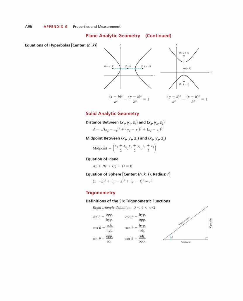
A96 APPENDIX G Properties and Measurement
Solid Analytic Geometry
Distance Between and
Midpoint Between and
Midpoint
Equation of Plane
Equation of Sphere Center: h, k, l , Radius: r
Trigonometry
Definitions of the Six Trigonometric Functions
Right triangle definition:
cot �adj.opp.
tan �opp.adj.
sec �hyp.adj.
cos �adj.hyp.
csc �hyp.opp.
sin �opp.hyp.
0 < < ��2
�x � h�2 � �y � k�2 � �z � l�2 � r2
��
Ax � By � Cz � D � 0
� �x1 � x2
2,
y1 � y2
2,
z1 � z2
2 ��x2, y2, z2��x1, y1, z1�
d � ��x2 � x1�2 � �y2 � y1�2 � �z2 � z1�2
�x2, y2, z2��x1, y1, z1�
Adjacent
Opp
osite
Hypotenuse
θ
Equations of Hyperbolas Center: h, k
�y � k�2
a2 ��x � h�2
b2 � 1�x � h�2
a2 ��y � k�2
b2 � 1
x
(h, k + c)
(h, k − c)
(h, k)
y
x
(h − c, k) (h + c, k) (h, k)
y��
Plane Analytic Geometry (Continued)
1053715_App_G.1.qxp 11/5/08 1:27 PM Page A96

APPENDIX G.1 Review of Algebra, Geometry, and Trigonometry A97
Circular function definition: is any angle and is a point on the terminal ray of the angle.
Signs of the Trigonometric Functions by Quadrant
Trigonometric Identities
Reciprocal identities
Pythagorean identities
Reduction formulas
tan � tan� � ��cos � �cos� � ��sin � �sin� � ��tan�� � � �tan cos�� � � cos sin�� � � �sin
cot2 � 1 � csc2 tan2 � 1 � sec2 sin2 � cos2 � 1
cot � cos sin
tan �sin cos
cot �1
tan sec �
1cos
csc �1
sin
tan �1
cot cos �
1sec
sin �1
csc
cot �xy
tan �yx
sec �rx
cos �xr
csc �ry
sin �yr
�x, y)
x
(x, y)
x
yr
θ
r = x2 + y2
y
Quadrant sin cos tan cot sec csc
I � � � � � �
II � � � � � �
III � � � � � �
IV � � � � � �
1053715_App_G.1.qxp 11/5/08 1:27 PM Page A97

A98 APPENDIX G Properties and Measurement
Trigonometry (Continued)
Sum or difference of two angles
Double-angle identities
Multiple-angle identities
Half-angle identities
Product identities
cos sin � �12
sin� � �� �12
sin� � ��
sin cos � �12
sin� � �� �12
sin� � ��
cos cos � �12
cos� � �� �12
cos� � ��
sin sin � �12
cos� � �� �12
cos� � ��
cos2 �12
�1 � cos 2 �
sin2 �12
�1 � cos 2 �
tan 4 �4 tan � 4 tan3
1 � 6 tan2 � tan4
cos 4 � 8 cos4 � 8 cos2 � 1
sin 4 � 4 sin cos � 8 sin3 cos
tan 3 �3 tan � tan3
1 � 3 tan2
cos 3 � �3 cos � 4 cos3
sin 3 � 3 sin � 4 sin3
tan 2 �2 tan
1 � tan2
cos 2 � 2 cos2 � 1 � 1 � 2 sin2
sin 2 � 2 sin cos
cos� � �� cos� � �� � cos2 � sin2 �
sin� � �� sin� � �� � sin2 � sin2 �
tan� ± �� �tan ± tan �
1 � tan tan �
cos� ± �� � cos cos � � sin sin �
sin� ± �� � sin cos � ± cos sin �
1053715_App_G.1.qxp 11/5/08 1:27 PM Page A98

APPENDIX G.1 Review of Algebra, Geometry, and Trigonometry A99
Library of Functions
Algebraic Functions
Linear or First-Degree Quadratic or Second-Degree Cubic or Third-DegreePolynomial Polynomial Polynomial
Fourth-Degree Polynomial Fifth-Degree Polynomial
Rational Function Rational Function Rational Function
Square Root Function Cube Root Functionf �x� � 3�xf�x� � �x
x−2 −1 1 2
−2
1
2
y
x1 2 3 4
1
2
3
4
y
f �x� �x2 � 1
xf �x� �
5x2 � 4
f �x� �x � 1x � 2
x42−4 −2
2
4
y
x4−4
2
4
y
x−2 4 6
2
4
−2
−4
y
f�x� � x5f�x� � x4
x−2 1 2
−2
−1
1
2
y
x−2 −1 1 2
1
2
3
4
y
f�x� � x3f�x� � x2f�x� � x
x−2 1 2
−2
−1
1
2
y
x−2 −1 1 2
1
2
3
4
y
x−2 −1 1 2
−2
−1
1
2
y
1053715_App_G.1.qxp 11/5/08 1:27 PM Page A99

A100 APPENDIX G Properties and Measurement
Library of Functions (Continued)
Exponential and Logarithmic Functions
Exponential Function Exponential Function Logarithmic Function
Trigonometric Functions
Sine Function Cosine Function Tangent Function
Cosecant Function Secant Function Cotangent Function
Nonelementary Functions
Absolute Value Function Compound Function Step Function
f �x� � x�f �x� � �1 � x,�x � 1,
x < 1 x ≥ 1
f �x� � �x�
x−2 −1 21
1
2
y
x42−2
−2
4
y
x−2 −1 1 2
1
2
3
4
y
f�x� � cot xf �x� � sec xf�x� � csc x
x
4
2
y
π π2
ππ2
−−x
ππ−
4
y
x
4
2
y
ππ2
−
f�x� � tan xf �x� � cos xf�x� � sin x
xππ−
4
2
y
x
−2
−1
2
y
π π π2
2x
π π π2
2
2
−2
1
y
f�x� � ln xf �x� � ax, 0 < a < 1f �x� � ax, a > 1
x1 2 3 4
1
2
−2
−1
y
x
y
x
y
1053715_App_G.1.qxp 11/5/08 1:27 PM Page A100

APPENDIX G.2 Units of Measurements A101
G.2 Units of MeasurementsUnits of Measurement of Length • Units of Measurement of Area • Units of Measurement of Volume •Units of Measurement of Mass and Force • Units of Measurement of Temperature • Miscellaneous Units and Number Constants
Units of Measurement of Length
English System: Inch in. , Foot ft , Yard yd , Mile mi
Metric System: Millimeter mm , Centimeter cm , Meter m ,Kilometer km
Conversion Factors six significant figures
Metric to English English to Metric
Miscellaneous
1 fathom
1 astronomical unit (average distance between earth and sun)
1 light-year (distance traveled by light in 1 year)
Units of Measurement of Area
English System: Square Inch in. , Square Foot ft , Square Yard yd ,Acre, Square Mile
Metric System: Square Centimeter cm , Square Meter m , SquareKilometer km
1 m2 � 10,000 cm21 km2 � 1,000,000 m2
�2��2��2�
1 ft2 � 144 in.21 yd2 � 9 ft21 acre � 43,560 ft21 mi2 � 640 acres
�mi2��2��2��2�
� 5,880,000,000,000 mi
� 93,000,000 mi
� 6 ft
1 mi � 1.60934 km1 km � 0.621371 mi
1 yd � 0.914400 m1 m � 1.09361 yd
1 ft � 0.304800 m1 m � 3.28084 ft
1 in. � 2.54000 cm1 cm � 0.393701 in.
1 in. � 25.4000 mm1 mm � 0.0393701 in.
��
1 cm � 10 mm1 m � 1000 mm
1 m � 100 cm1 km � 1000 m
��������
1 ft � 12 in.1 yd � 3 ft
1 mi � 1760 yd1 mi � 5280 ft
��������
1053715_App_G.2.qxp 11/5/08 1:28 PM Page A101

A102 APPENDIX G Properties and Measurement
Units of Measurement of Area (Continued)
Conversion Factors six significant figures
Metric to English English to Metric
Miscellaneous
1 square mile section quarters
Units of Measurement of Volume
English System: Cubic Inch in. , Cubic Foot ft , Cubic Yard yd , Fluid Ounce fl oz , Pint pt , Quart qt , Gallon gal
Metric System: Cubic Centimeter cm or cc , Cubic Meter m , MillilitermL , Liter
Conversion Factors six significant figures
Metric to English English to Metric
Miscellaneous
1 barrel �bl� � 42 gallons �petroleum�1 tablespoon � 3 teaspoons
1 cup � 16 tablespoons1 quart � 4 cups
1 fifth � 0.757 liter1 gallon � 5 fifths
1 yd3 � 0.764555 m31 m3 � 1.30795 yd3
1 ft3 � 0.0283168 m31 m3 � 35.3147 ft31 in.3 � 16.3871 cm31 cm3 � 0.0610237 in.3
��
1 cm3 � 1 cc � 1 mL
1 liter � 1000 mL1 m3 � 1000 liters
���3��3�
1 ft3 � 7.48052 gal1 gal � 231 in.31 pt � 16 fl oz1 qt � 32 fl oz
1 qt � 2 pt1 gal � 4 qt
1 ft3 � 1728 in.31 yd3 � 27 ft3���������3��3��3�
� 4� 1
1 mi2 � 2.58999 km21 km2 � 0.386102 mi21 yd2 � 0.836127 m21 m2 � 1.19599 yd2
1 ft2 � 0.0929030 m21 m2 � 10.7640 ft21 in.2 � 6.45160 cm21 cm2 � 0.155000 in.2
��
1053715_App_G.2.qxp 11/5/08 1:28 PM Page A102
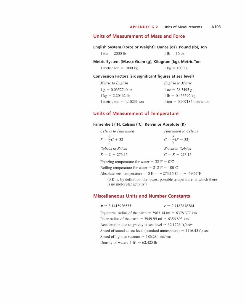
APPENDIX G.2 Units of Measurements A103
Units of Measurement of Mass and Force
English System Force or Weight : Ounce oz , Pound lb , Ton
Metric System Mass : Gram g , Kilogram kg , Metric Ton
Conversion Factors six significant figures at sea level
Metric to English English to Metric
Units of Measurement of Temperature
Fahrenheit F , Celsius C , Kelvin or Absolute K
Celsius to Fahrenheit Fahrenheit to Celsius
Celsius to Kelvin Kelvin to Celsius
Freezing temperature for water
Boiling temperature for water
Absolute zero temperature
is, by definition, the lowest possible temperature, at which thereis no molecular activity.
Miscellaneous Units and Number Constants
Equatorial radius of the earth 3963.34 mi 6378.377 km
Polar radius of the earth 3949.99 mi 6356.893 km
Acceleration due to gravity at sea level 32.1726
Speed of sound at sea level (standard atmosphere) 1116.45
Speed of light in vacuum 186,284
Density of water: 1 ft3 � 62.425 lb
mi�sec�ft�sec�
ft�sec2���
��
e � 2.7182818284� � 3.1415926535
��0 K
� 0 K � �273.15�C � �459.67�F
� 212�F � 100�C
� 32�F � 0�C
C � K � 273.15K � C � 273.15
C �59
�F � 32�F �95
C � 32
��������
1 ton � 0.907185 metric ton1 metric ton � 1.10231 ton
1 lb � 0.453592 kg1 kg � 2.20462 lb
1 oz � 28.3495 g1 g � 0.0352740 oz
��
1 kg � 1000 g1 metric ton � 1000 kg
������
1 lb � 16 oz1 ton � 2000 lb
������
1053715_App_G.2.qxp 11/5/08 1:28 PM Page A103

A104 APPENDIX H Graphing Utility Programs
H Graphing Utility Programs
Programs for graphing calculators are referenced inseveral sections in the text. This appendix containstranslations of these programs for the TI-82, TI-83,TI-83 Plus, TI-84 Plus, TI-86, TI-89, TI-92, TI-92 Plus,and Voyage 200, arranged by calculator model. Similarprograms can be written for other brands and models ofgraphing calculators.
Enter a program in your calculator, then refer to thetext discussion and apply the program as appropriate.The following section references are provided to helpyou locate the text discussions of the programs and theiruses.
Evaluating Functions Section 2.4
Midpoint Rule Section 11.6
Simpson’s Rule Section 12.4
Newton’s Method Section 15.8
Texas Instruments TI-82 ,TI-83,TI-83Plus, and TI-84 Plus
Evaluating Functions
This program evaluates a function that has been storedin Y1.
PROGRAM:EVALUATE:Lbl 1:Input “ENTER X”, X:Disp Y1
:Goto 1
To use this program, enter a function in Y1. Then runthe program—it will allow you to evaluate the functionat several values of
Midpoint Rule
This program uses the Midpoint Rule to approximatethe definite integral You must store the function as Y1 before executing the program. Theprogram itself will prompt you for the limits of a and band for the number of subintervals n.
PROGRAM:MIDPOINT:Disp “LOWER LIMIT”:Input A:Disp “UPPER LIMIT”:Input B:Disp “N DIVISIONS”:Input N:0→S:(B-A)/N→W:1→J:Lbl 1:A+(J-1)W→L:A+JW→R:(L+R)/2→X:S+WY1→S:IS>(J, N):Goto 1:Disp “APPROXIMATION”:Disp S
f �x��b
a f �x� dx.
x.
1053715_App_H.qxp 11/5/08 1:29 PM Page A104
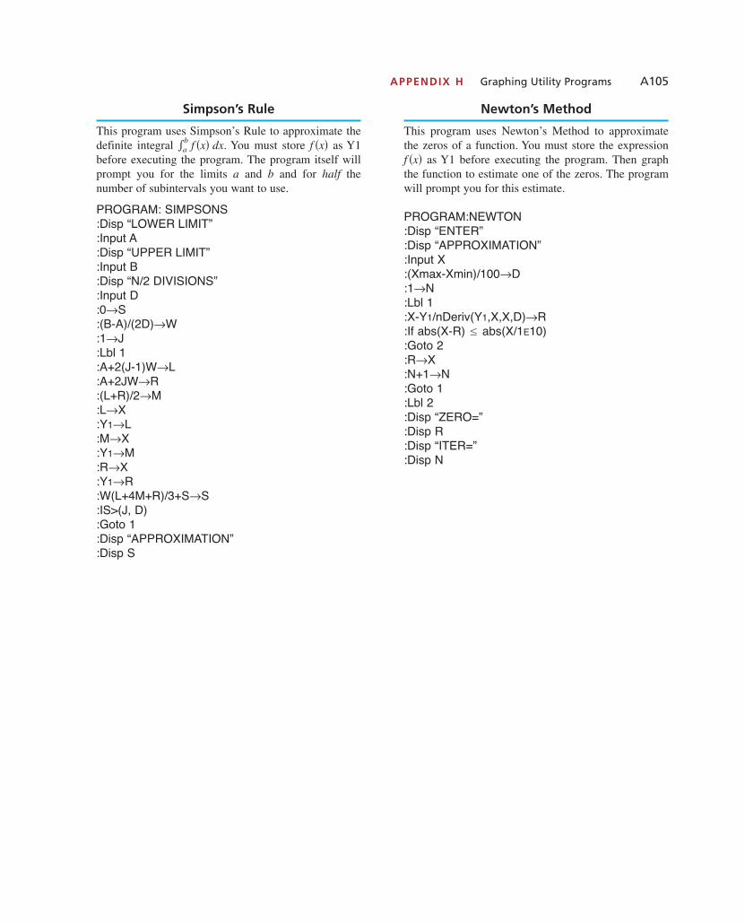
APPENDIX H Graphing Utility Programs A105
Simpson’s Rule
This program uses Simpson’s Rule to approximate thedefinite integral You must store as Y1before executing the program. The program itself willprompt you for the limits a and b and for half the number of subintervals you want to use.
PROGRAM: SIMPSONS:Disp “LOWER LIMIT”:Input A:Disp “UPPER LIMIT”:Input B:Disp “N/2 DIVISIONS”:Input D:0→S:(B-A)/(2D)→W:1→J:Lbl 1:A+2(J-1)W→L:A+2JW→R:(L+R)/2→M:L→X:Y1→L:M→X:Y1→M:R→X:Y1→R:W(L+4M+R)/3+S→S:IS>(J, D):Goto 1:Disp “APPROXIMATION”:Disp S
Newton’s Method
This program uses Newton’s Method to approximatethe zeros of a function. You must store the expression
as Y1 before executing the program. Then graphthe function to estimate one of the zeros. The programwill prompt you for this estimate.
PROGRAM:NEWTON:Disp “ENTER”:Disp “APPROXIMATION”:Input X:(Xmax-Xmin)/100→D:1→N:Lbl 1:X-Y1/nDeriv(Y1,X,X,D)→R:If abs(X-R) abs(X/1E10):Goto 2:R→X:N+1→N:Goto 1:Lbl 2:Disp “ZERO=”:Disp R:Disp “ITER=”:Disp N
≤
f �x�f �x��b
a f �x� dx.
1053715_App_H.qxp 11/5/08 1:29 PM Page A105

A106 APPENDIX H Graphing Utility Programs
Texas Instruments TI-86
Evaluating Functions
This program evaluates a function that has been storedas y1.
:PROGRAM:Evaluate:Repeat 1<0:Input x:Disp y1:End
Midpoint Rule
This program uses the Midpoint Rule to approximatethe definite integral You must store theexpression as y1 before executing the program. Theprogram itself will prompt you for the limits a and band for the number of subintervals n.
PROGRAM:MIDPOINT:Disp “LOWER LIMIT”:Input A:Disp “UPPER LIMIT”:Input B:Disp “n DIVISIONS”:Input N:0→S:(B-A)/N→W:1→J:While J≤N:A+(J-1) W→L:A+J W→R:(L+R)/2→x:S+W y1→s:J+1→J:End:Disp “APPROXIMATION”:Disp S
Simpson’s Rule
This program uses Simpson’s Rule to approximate the definite integral You must store theexpression as y1 before executing the program. Theprogram itself will prompt you for the limits a and band for half the number of subintervals you want to use.
:PROGRAM:SIMPSON:Disp “LOWER LIMIT”:Input A:Disp “UPPER LIMIT”:Input B:Disp “n/2 DIVISIONS”:Input D:0→S:(B-A)/(2D)→W:1→J:While J≤D:A+2(J-1) W→L:A+2J W→R:(L+R)/2→M:L→x:y1→L:M→x:y1→M:R→x:y1→R:W (L+4M+R)/3+S→S:J+1→J:End:Disp “APPROXIMATION”:Disp S
*
**
f �x��b
a f �x� dx.
*
**
f �x��b
a f �x� dx.
1053715_App_H.qxp 11/5/08 1:29 PM Page A106
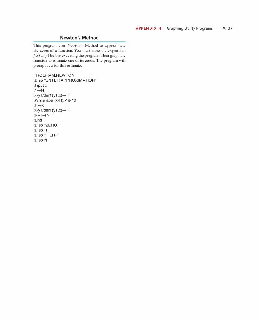
APPENDIX H Graphing Utility Programs A107
Newton’s Method
This program uses Newton’s Method to approximatethe zeros of a function. You must store the expression
as y1 before executing the program. Then graph thefunction to estimate one of its zeros. The program willprompt you for this estimate.
PROGRAM:NEWTON:Disp “ENTER APPROXIMATION”:Input x:1→N:x-y1/der1(y1,x)→R:While abs (x-R)>1E-10:R→x:x-y1/der1(y1,x)→R:N+1→N:End:Disp “ZERO=”:Disp R:Disp “ITER=”:Disp N
f �x�
1053715_App_H.qxp 11/5/08 1:29 PM Page A107

A108 APPENDIX H Graphing Utility Programs
Texas Instruments TI-89, TI-92, TI-92Plus, and Voyage 200
Evaluating Functions
This program evaluates a function that has been storedas y1( ).
:evaluate ( ):Prgm:Loop:Input “Input x”, x:Disp y1(x):End Loop:End Prgm
Midpoint Rule
This program uses the Midpoint Rule to approximatethe definite integral You must store theexpression as y1(x) before executing the program.The program itself will prompt you for the limits and
and for the number of subintervals
:midpoint ( ):Prgm:Input “Lower Limit”, a:Input “Upper Limit”, b:Input “n Divisions”, n:0→s:(b-a)/n→w:1→i:While i≤n:a+(i-1) w→l:a+i w→r:(l+r)/2→x:s+w y1(x)→s:i+1→i:EndWhile:Disp “Approximation”:Disp s:EndPrgm
Simpson’s Rule
This program uses Simpson’s Rule to approximate the definite integral You must store theexpression as y1(x) before executing this program.The program itself will prompt you for the limits a andb and for half the number of subintervals you want to use.
:simpson( ):Prgm:Input “Lower Limit”, a:Input “Upper Limit”, b:Input “n/2 Divisions”, d:0→s:(b-a)/(2 d)→w:1→i:While i≤d:a+2 (i-1) w→l:a+2 i w→r:(l+r)/2→m:l→x:y1(x)→l:m→x:y1(x)→m:r→x:y1(x)→r:w (1+4 m+r)/3+s→s:i+1→i:EndWhile:Disp “Approximation”:Disp s:EndProgram
**
****
*
f �x��b
a f�x� dx.
*
**
n.ba
f �x��b
a f�x� dx.
x
1053715_App_H.qxp 11/5/08 1:29 PM Page A108
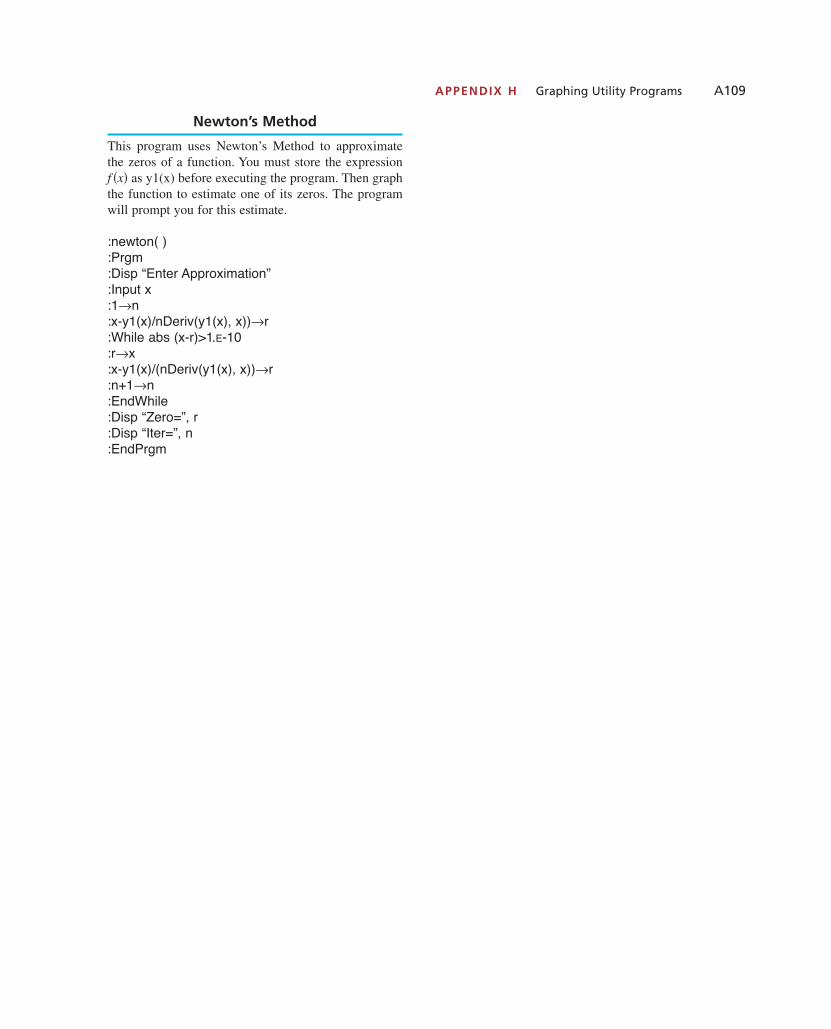
APPENDIX H Graphing Utility Programs A109
Newton’s Method
This program uses Newton’s Method to approximatethe zeros of a function. You must store the expression
as y1(x) before executing the program. Then graphthe function to estimate one of its zeros. The programwill prompt you for this estimate.
:newton( ):Prgm:Disp “Enter Approximation”:Input x:1→n:x-y1(x)/nDeriv(y1(x), x))→r:While abs (x-r)>1.E-10:r→x:x-y1(x)/(nDeriv(y1(x), x))→r:n+1→n:EndWhile:Disp “Zero=”, r:Disp “Iter=”, n:EndPrgm
f �x�
1053715_App_H.qxp 11/5/08 1:29 PM Page A109