an introduction to geometrical modelling and mesh...

An introduction to geometrical modelling andmesh generation with Gmsh

Christophe Geuzaine Jean-Francois Remacle

November 4, 2008

Contents

1 Introduction 51.1 The Design of Gmsh . . . . . . . . . . . . . . . . . . . . . . . 6

1.1.1 Fast and Light . . . . . . . . . . . . . . . . . . . . . . 71.1.2 User-friendly . . . . . . . . . . . . . . . . . . . . . . . 8

2 Computational Geometry Toolbox 112.1 Delaunay and Voronoı . . . . . . . . . . . . . . . . . . . . . . 11

2.1.1 The Voronoı diagram . . . . . . . . . . . . . . . . . . . 112.1.2 The Delaunay Triangulation . . . . . . . . . . . . . . . 142.1.3 Construction of Delaunay Triangulations . . . . . . . . 21

2.2 Nearest neighbors . . . . . . . . . . . . . . . . . . . . . . . . . 312.3 Point location . . . . . . . . . . . . . . . . . . . . . . . . . . . 31

3 Solid Models 333.1 Boundary Representation of Solids . . . . . . . . . . . . . . . 33

3.1.1 Geometrical Description . . . . . . . . . . . . . . . . . 393.2 Discrete Representation of the Geometry . . . . . . . . . . . . 49

3.2.1 Harmonic maps . . . . . . . . . . . . . . . . . . . . . . 49

4 Mesh Generation 574.1 Generalities . . . . . . . . . . . . . . . . . . . . . . . . . . . . 57

4.1.1 The Euler-Poincare Formula . . . . . . . . . . . . . . . 584.1.2 Mesh generation procedure . . . . . . . . . . . . . . . . 62

4.2 Mesh size field and quality measures . . . . . . . . . . . . . . 644.2.1 Mesh size field . . . . . . . . . . . . . . . . . . . . . . . 64

4.3 One Dimensional Meshing . . . . . . . . . . . . . . . . . . . . 664.4 Planar Meshing . . . . . . . . . . . . . . . . . . . . . . . . . . 674.5 Surface Meshing . . . . . . . . . . . . . . . . . . . . . . . . . . 67

3

4 CONTENTS

4.6 Quadrilateral Meshing . . . . . . . . . . . . . . . . . . . . . . 674.7 Tetrahedral Meshing . . . . . . . . . . . . . . . . . . . . . . . 674.8 Hexaedral Meshing . . . . . . . . . . . . . . . . . . . . . . . . 674.9 Mesh Data Structures . . . . . . . . . . . . . . . . . . . . . . 674.10 Structured and Hybrid Mesh Generation . . . . . . . . . . . . 67

4.10.1 Hyperbolic mesh generation . . . . . . . . . . . . . . . 674.10.2 Elliptic mesh generation . . . . . . . . . . . . . . . . . 674.10.3 Boundary Layer Meshing . . . . . . . . . . . . . . . . . 67

4.11 Mesh Adaptation . . . . . . . . . . . . . . . . . . . . . . . . . 674.11.1 Local Mesh Modifications . . . . . . . . . . . . . . . . 674.11.2 Interactions with a solver . . . . . . . . . . . . . . . . . 67

4.12 High Order Mesh Generation . . . . . . . . . . . . . . . . . . 67

Chapter 1

Introduction

When we started the Gmsh project in the summer of 1996, our goal was todevelop a fast, light and user-friendly software to easily create geometries andmeshes that could be used in our three-dimensional finite element solvers [?],and then visualize and export the computational results with maximum flex-ibility. At the time, no open-source software combining a CAD engine, amesh generator and a post-processor was available: the existing integratedtools were expensive commercial packages [?], and the freeware or sharewaretools were limited to either CAD [?], two-dimensional mesh generation [?],three-dimensional mesh generation [?, ?, ?], or post-processing [?]. The needfor a free integrated solution was conspicuous, and several projects similarin spirit to Gmsh were also born around the same time—some of them stillactively developed today [?, ?]. Gmsh however was unique in its design: itconsisted of a very small kernel with four modules (geometry, mesh, solverand post-processing), not tied to any particular computational solver, anddesigned from the start to be driven both using a user-friendly graphicalinterface (GUI) and its own scripting language.

The first public release of Gmsh occurred in 1998. This version wasUnix-only, distributed over the internet in binary form, with the graphicslayer based on OpenGL [?] and the user interface written in Motif [?]. Afterseveral updates and a short-lived Windows-only fork in 2000, the whole userinterface was rewritten using FLTK [?] in early 2001, and the code, still inbinary-only form, was released for Windows and a variety of Unix operatingsystems. In 2003 the full source code was released under the GNU GeneralPublic License [?], and it was modified to provide native support for all majoroperating systems: Windows, MacOS and all Unix/X11 variants. In the

5

6 CHAPTER 1. INTRODUCTION

summer of 2006 Gmsh underwent a major rewrite, which led to the releaseof version 2 of the software in February 2007. About 50% of the code inversion 2 is new: an abstract geometrical and post-processing layer has beenintroduced, the mesh data structures and algorithms have been rewrittenfrom scratch, and the graphics layer has also been completely overhauled.

Today Gmsh enjoys a thriving community of several hundred users anddevelopers worldwide. It is driven by the need of researchers and engineers inacademia and industry alike for a small, open-source pre- and post-processingsolution for grid-based numerical methods. The aim of this paper is not to bea user’s guide or a reference manual—see [?] instead. Rather, it is to presentthe philosophy and the original features of Gmsh which make it stand outfrom its free and commercial alternatives.

The paper is structured as follows. In Section 1.1 we outline the overallphilosophy and design goals of Gmsh, as well as the main technical choicesthat were made in order to achieve these goals. Sections ??, ??, ?? and ??then respectively describe the geometry, mesh, solver and post-processingmodules. The paper is concluded in Section ?? with perspectives for futuredevelopments.

1.1 The Design of Gmsh

Gmsh is built around four modules: geometry, mesh, solver and post-processing.Each module can be controlled either interactively using the GUI or usingthe scripting language.

The design of all four modules relies on a simple philosophy—be fast,light and user-friendly.

Fast: on a standard personal computer at any given point in time Gmshshould launch instantaneously, be able to generate a “larger than aver-age” mesh (compared to the standards of the finite element community;say, one million tetrahedra in 2008) in less than a minute, and be able tovisualize such a mesh together with associated post-processing datasetsat interactive speeds.

Light: the memory footprint of the application should be minimal and thesource code should be small enough so that a single developer canunderstand it. Installing or running the software should not depend onany non-widely available third-party software package.

1.1. THE DESIGN OF GMSH 7

User-friendly: the graphical user interface should be designed in such a waythat a new user can create simple meshes in a matter of minutes. Inaddition, the code should be robust, portable, scriptable, extensible andthoroughly documented—all features contributing to a user-friendlyexperience.

In the following sections we describe the technical choices that we made toachieve these sometimes conflicting design objectives. Although major partsof the code have been rewritten over the years, the overall initial architectureand design from 1996 have always stayed the same.

1.1.1 Fast and Light

In order to be fast and light in the sense just described above, Gmsh is entirelywritten in standard C++ [?]—both the kernel and the user interface.

The kernel uses BLAS [?] (through the GSL, the GNU Scientific Li-brary [?]) for most of the basic linear algebra. To keep them easy to under-stand the algorithms have not been overly optimized for speed or memoryusage, yet Gmsh currently generates about a million tetrahedra per minuteand per 150 Mb of RAM on a standard personal computer, which makes itpowerful enough for many academic and engineering applications.

The graphical interface is built using FLTK [?] and OpenGL [?]. UsingFLTK instead of a larger or more complex widget toolkit, like for exam-ple Java, TCL/TK, GTK or QT, allows to link Gmsh statically with thetoolkit. This tremendously reduces the launch time, memory footprint andinstallation complexity (installing Gmsh requires copying a single executablefile), as well as the build time—a statically linked, ready to use executable isproduced in a few minutes on a standard personal computer. Analogously,directly using OpenGL instead of a more complex graphics library like In-ventor [?] or VTK [?] makes Gmsh lightweight, without sacrificing renderingperformance (Gmsh makes extensive use of OpenGL vertex arrays).

The design of the solver and scripting interfaces follows the same strat-egy: the solver interface is written using standard Unix and TCP/IP socketsinstead of, e.g., Corba [?], and the scripting interface is built using Lex/Flexand Yacc/Bison [?] instead of using an external scripting language like, e.g.,Python.


1.1.2 User-friendly

Although Gmsh can be built as a library (which can then be linked with othersoftware tools), it is usually distributed as a stand-alone software, ready tobe used by end users. This stand-alone version can be run either interactivelyusing the graphical user interface or in a non-interactive mode—either fromthe command line or via the scripting language.

Achieving “user-friendliness” has been an important driving factor behindkey technical choices. We detail some of these choices hereafter, focusing onthe list of desirable features given at the beginning of the section.

Robustness and Portability

To achieve robustness, i.e., working for the largest possible range of inputdata and being as tolerant as possible to erroneous user input, we use robustgeometrical predicates [?] in critical portions of the algorithms, and strive toprovide useful error messages when an unmanageable exception is triggered.

In order to easily produce a native version of the code on all majoroperating systems, Gmsh is written entirely in standard C++, and usesportable toolkits for its GUI (FLTK) and graphics rendering (OpenGL).Open-sourcing Gmsh under the GNU General Public License [?] also helpedportability, as the code was made part of several official Linux distributions(most notably Debian [?]), and thus benefited from their extensive auto-mated testing infrastructure. Either with the graphical user interface or inbatch mode, the same version of Gmsh now runs on most computers, fromlaptops to workstations and large HPC clusters.

Scriptability

Gmsh is scriptable so that all input data can be parametrized, and so thatGmsh can be easily inserted as a component inside a larger computationalchain. As mentioned above, scripting is implemented in Gmsh using Lexand Yacc. The tight integration with the resulting language means that fullaccess to internal capabilities is provided, including bidirectional access tomore than 500 internal options fine-tuning the behaviour of the four modules.The scripting language allows for example to fully parametrize all geometricalentities, to interface external solvers without modifying the source code, or toautomate all post-processing operations, e.g., to create complex animationsor perform off-screen rendering [?].

1.1. THE DESIGN OF GMSH 9

Extensibility

We tried to ease the modification and addition of features by users and devel-opers. Such extensibility takes different forms for each of the four modules:

Geometry: the abstract, object-oriented geometry layer permits to writeall the algorithms independently of the underlying CAD representa-tion. At the source code level Gmsh is thus easily extensible by addingsupport for additional CAD engines. Currently two engines are inter-faced: the native Gmsh CAD engine and OpenCascade [?]. Addingsupport for other engines like, e.g., Parasolid [?], can be done simplyby deriving four abstract classes—see Section ??. At the scripting levelusers can then transparently mix and match geometrical parts repre-sented internally by different CAD engines. For example, it is possibleto extend an OpenCascade model of an airplane with a terrain modeldefined in the scripting language.

Mesh: using the abstract geometrical interface it is also possible to interfaceadditional meshing kernels. Currently, in addition to its own meshingalgorithms (see Section ??), Gmsh is interfaced with Netgen [?] andTetgen [?].

Solver: a socket-based communication interface allows to interface Gmshwith various solvers without changing the source code; tailored graph-ical user interfaces can also easily be added when more fine-grainedinteractions are needed.

Post-processing: the post-processor can be extended with user-defined op-erations through dynamically loadable plug-ins. These plug-ins act onpost-processing datasets (called views) in one of two ways: either de-structively changing the contents of a view, or creating one or moreviews based on the current view.

All source code-level extensions can be enabled or disabled at compile timethanks to an autoconf-based build mechanism [?], which selects which partsof the code to include/exclude.

Documentation and Open File Formats

Documentation is provided both in the source code and in the form of areference manual, including several hands-on tutorial examples and a com-


prehensive web site with several mailing lists and a wiki.Another important feature contributing to user-friendliness is the avail-

ability of standard input and output file formats. Gmsh uses open or defacto standard formats whenever possible, from standard bitmap graphicsformats (JPEG, GIF, PNG) and vector formats [?] (SVG, PostScript, PDF)to mesh formats (Ideas UNV, Nastran BDF). Combined with the open-sourcerelease of the code this greatly facilitates the integration of Gmsh with othercomputational tools.

Chapter 2

Computational GeometryToolbox

2.1 Delaunay and Voronoı

2.1.1 The Voronoı diagram

Let p1 and p2 be two points of R2. The mediator M(p1,p2) is the locus ofall the points which are equidistant to p1 and p2:

M(p1,p2) = p ∈ R2, d(p,p1) = d(p,p2)

where d(., .) is the euclidian distance between two points of R2, i.e.

d2(p1,p2) = (p2 − p1) · (p2 − p1). (2.1)

The equation of the mediator can be found out using this definition

(p1 − p) · (p1 − p) = (p2 − p) · (p2 − p)

or

(p1 − p2) ·

p− 1

2(p1 + p2)︸︷︷︸

pm

= 0

This shows that the mediator is the orthogonal bissector of the straight edgelinking the two points. The mediator separates the plane into two regions.

11

12 CHAPTER 2. COMPUTATIONAL GEOMETRY TOOLBOX

pmp1

M

p2

p

Figure 2.1: The mediator.

The first region contains all the points that are closer to p1, the second onecontains the ones that are closer to p2. Any point of R2/M can be associatedto one of those two points.

Let us consider a set of N points S = p1, . . . ,pN. More specifically,we assume that the points are in general position, by which we mean nofour points are cocircular. The Voronoı cell C(pi) associated to point piis the locus of points of R2 that are closer to pi than any other point pj,j = 1, . . . , N , i 6= j.

The Voronoı cell is constructed as follow. Consider all mediatorsM(pi,pj).Each of those mediators define a half plane. The Voronoı diagram is the partof the space that is always closer to pi, i.e. that always associate pi to thepoint p, for all possible mediators.(see Figure 2.2). The set of all Voronoıcells is called the Voronoı diagram of S (see Figure 2.2).

Let us present some remarkable properties of the Voronoı diagram.

Property 2.1.1 Voronoı cells are convex polytopes.

By definition, each Voronoi region C(pi) is the intersection of open half planescontaining vertex pi. Therefore, C(pi) is open and convex. Different Voronoıregions are disjoint. Voronoı cells are polygons in 2D, polyhedra in 3D andd-polytopes in dD. Voronoı cells are either closed or open. They can onlybe open for points that are located on the convex hull of the 2D domain. Apoint pi of S lies on the convex hull of S if and only if its Voronoı cell C(pi)is unbounded.

2.1. DELAUNAY AND VORONOI 13

pi

pj

pk

vI

C(pi)

Figure 2.2: The Voronoı diagram. The Voronoı cell C(pi) relative to vertexpi is coloured.


Figure 2.3: Two triangulations of S, both containing nt = 13 triangles.

Property 2.1.2 Voronoı points vI are always located at intersection of 3mediators.

Property 2.1.2 is only true if there exist no quadruplets of points in S thatare cocircular. If such a set exists, it may happen that a vertex of the Voronoıis at the the intersection of more than 3 mediators. Consider the example ofFigure 2.2 where vi is at the intersecion of C(pi), C(pj) and C(pk). Voronoıpoint vI is loacted at the center of the unique circle passing through pi, pjand pk.

2.1.2 The Delaunay Triangulation

We first define what is a triangulation of S: it is a planar subdivision whosebounded faces are triangles and whose vertices are the points pi of S. Notethat all triangulations do not cover the same subset of R2. In what follows,we consider that the domain to triangulate is the convex hull of S.

Even with the same domain to cover, several triangulations are possible(see Figure 2.3). Yet, every triangulation has the same number of trianglesand edges!

Property 2.1.3 Let S be a set of N points in the plane, not all collinear,and let Nh denote the number of points in S that lie on the convex hull of


S. Then any triangulation of S has nt(N,Nh) = 2N − 2−Nh triangles andne(N,Nh) = 3N − 3−Nh edges.

Proof Consider first that all the points in S are in the convex hull: N = Nh.A triangulation consist simply in triangles tI(p1,pi,pi+1), i = 2, . . . , N − 1.The number of triangle is therefore nt = N − 2 wich is consistent with theformula. The number of edges in the triangulation is calculated as follows:Nh = N edges on the convex hull and N − 3 internal edges wich givesne = N +N − 3 = 2N − 3 which is again consistent with the proposition.

The rest of the proof works using a recurrence argument. Assume thatformulas are true for N . Let us now consider one new vertex pN+1 thatlies inside the convex hull. This new vertex lies inside one of the exist-ing triangles, say tI(pi,pj,pk). We remove tI and replace it by three newtriangles tJ(pi,pj,pN+1), tJ(pj,pk,pN+1), tJ(pk,pi,pN+1). We have there-fore nt(Nh, Nh) = Nh − 2 and nt(N + 1, Nh) = nt(N,Nh) + 2 which givesnt(N,Nh) = Nh − 2 + 2(N − Nh) = 2N − 2 − Nh. Similarly, three newedges have been added in the process. Then, ne(Nh, Nh) = 2Nh − 3 andne(N+1, Nh) = ne(N,Nh)+3 which gives ne(N,Nh) = 2Nh−3+3(N−Nh) =3N − 3−Nh.

Consider a triangulation T with nt triangles. This triangulation has 3ntinternal angles. Consider the vector of angles A(T ) = (α1, . . . , α3nt) sortedby increasing values. We can define such a vector for any triangulation of theconvex hull of the domain. Each of those vectors has the same length andit is therefore possible to compare them, e.g. lexicographically. We say thatone given triangulation T is angle-optimal if A(T ) ≤ A(T ′), ∀T ′. Accordingto that criterion, left triangulation of Figure 2.3 is better than the right one.

Angle-optimal trianglations have interresting interpolation properties andit is therefore useful to find methods that allow to construct such triangula-tions.

For a given set of points, the (unique) angle-optimal triangulation is thetriangulation that has the highest minimal angle. Let us see now how tobuild such a triangulation.

Consider now the edge e(p4,p6) of Figure 2.4. This edge is surrounded bytwo triangles t1(p4,p6,p1) and t2(p4,p6,p2) . An edge swap is a local meshmodification operator that consist in changing locally the triangulation by re-placing edge e(p4,p6) by e′(p1,p2). Triangles t1(p4,p6,p1) and t2(p4,p6,p2)are replaced by t′1(p1,p2,p4) and t′2(p1,p2,p6). Figure 2.4 illustrate the edgeswap operation.


t2α5

α6

t1

p2

p4

p6

p1

e

α1

α2

α3

α4 α3α′5

t1

e′

p2

p4

p6

p1

α1α′2

α′6

α′3

t′2

Figure 2.4: Edge swap.

It is indeed possible to use the edge swap operator in order to build angle-optimal triangulation. In that purpose, we can simply decide to swap edgee if

min (α1, . . . , α6) < min (α′1, . . . , α′6).

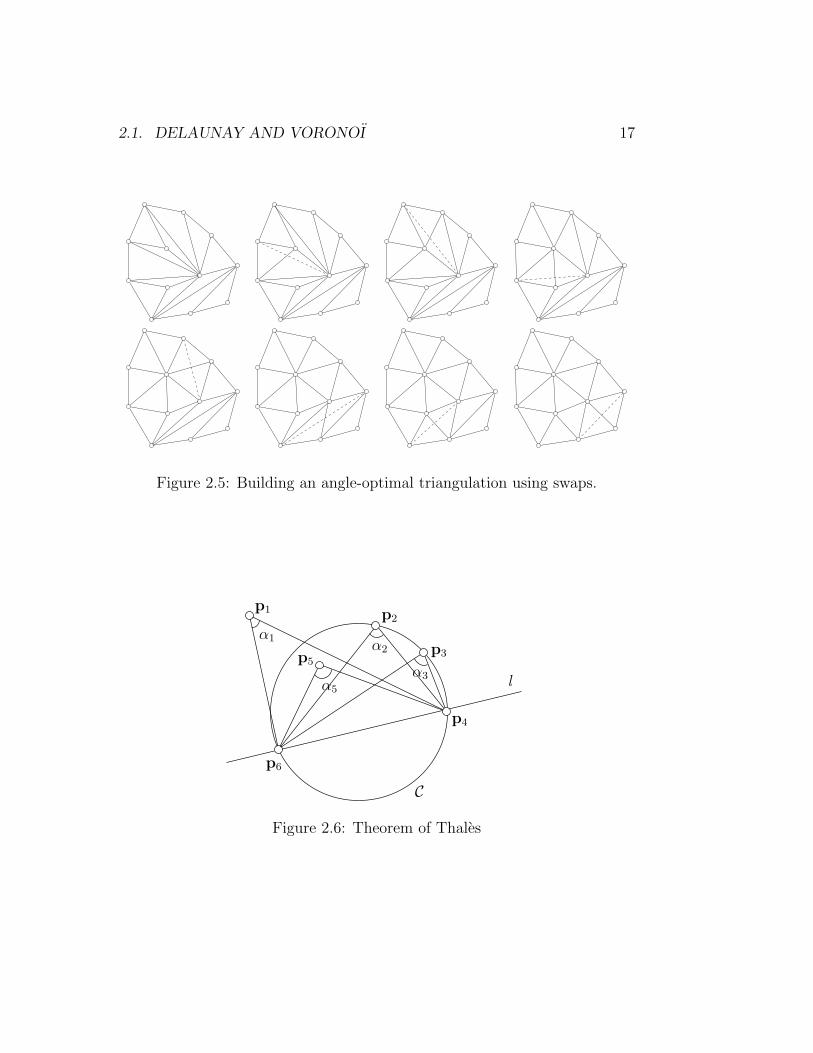
Such an edge is said invalid. Given a finite set of points, there is a finitenumber of possible triangulations. When the angle criterion is applied, everyedge swap produce a new triangulation that is better than the actual one.Therefore, building the angle-optimal triangulation consist in looping overall the edges of the mesh and swap them until the optimal configuration isattained i.e. when no invalid edges remain in the triangulation. Figure 2.5illustrate that procedure.

Yet, computing angles is a costly operation and it is possible to use asimpler and cheaper rule to verify the validity of an edge.

Property 2.1.4 Let C be a circle, l a line intersecting C in points p4 and p6

and p1, and p2, p3 and p5 points lying on the same side of l . Suppose thatp2 and p3 lie on C, that p5 lies inside C, and that p1 lies outside C. Then(see Fig. 2.6):

α1 < α2 = α3 < α5.

Property 2.1.5 [Lawson’s Criterion] Consider an edge e with its two neigh-boring triangles t1 and t2. Consider the circumcircle C of triangle t1 and pointp that belongs to t2 but not to t1. Edge e is invalid if p ∈ C.


Figure 2.5: Building an angle-optimal triangulation using swaps.

p6

p3p5

α2

α3α5

p1 p2

p4

α1

C

l

Figure 2.6: Theorem of Thales


C ′

α′

α

C

p2

p4

p6

p1

e

e′

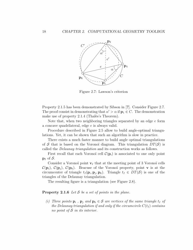
Figure 2.7: Lawson’s criterion

Property 2.1.5 has been demonstrated by Sibson in [?]. Consider Figure 2.7.The proof consist in demonstrating that α′ > α if p1 ∈ C. The demonstrationmake use of property 2.1.4 (Thales’s Theorem).

Note that, when two neighboring triangles separated by an edge e forma concave quadrilateral, edge e is always valid.

Procedure described in Figure 2.5 allow to build angle-optimal triangu-lations. Yet, it can be shown that such an algorithm is slow in practice.

There exists a much faster manner to build angle optimal triangulationsof S that is based on the Voronoı diagram. This triangulation DT (S) iscalled the Delaunay triangulation and its construction works as follows.

First recall that each Voronoı cell C(pi) is associated to one only pointpI of S.

Consider a Voronoı point vI that at the meeting point of 3 Voronoı cellsC(pi), C(pj), C(pk). Beacuse of the Voronoı property, point v is at thecircumcenter of triangle tI(pi,pj,pk). Triangle tI ∈ DT (S) is one of thetriangles of the Delaunay triangulation.

The resulting figure is a triangulation (see Figure 2.8).

Property 2.1.6 Let S be a set of points in the plane.

(i) Three points pi , pj and pk ∈ S are vertices of the same triangle tI ofthe Delaunay triangulation if and only if the circumcircle C(tI) containsno point of S in its interior.


Figure 2.8: The Voronoı diagram and its associated Delaunay triangulation


v′

p3

C(t)

la

lc

lbbc

v

t

ap1

p2

Figure 2.9: Illustration of why property (i) of 2.1.6 is true.

(ii) Two points pi and pj ∈ S form an edge eI of the Delaunay triangulationif and only if there is a closed disc C that contains pi and pj on itsboundary and does not contain any other point of S.

Proof Property (i) of 2.1.6, also called the incircle property, is a simpleconsequense of the properties of construction of the Voronoı diagram. Figure2.11 show one triangle t and its circumcenter v. If a point like a exist inS, triangle t is cannot be in the Delaunay triangulation because point a iscloser to v that at least one of the three points p1 p2 or p3. Therefore, asit is drawn in the Figure, mediator la crosses another mediator at point v′

inside the triangle, which is impossible.

Property 2.1.7 Let S be a set of points in the plane in general position.A triangulation T of S is angle-optimal if and only if T is the Delaunaytriangulation of S.

Proof We shall prove that the angle-optimal triangulation is the Delaunaytriangulation by contradiction. So assume T is a legal triangulation of Sthat is not a Delaunay triangulation. By Property (ii) of 2.1.6, this meansthat there is a triangle t(pi,pj,pk) such that the circumcircle C(t) containsa point pl ∈ S in its interior. Let e(pi,pj) be the edge of t′(pi,pj,pl) suchthat the triangle t′ does not intersect t. Of all such pairs (pi,pj,pk,pl) in T ,


choose the one that maximizes the angle pi,pl,pj. Now look at the trianglet′′(pi,pj,pm) adjacent to t along e. Since T is angle-optimal, e is legal.By Property 2.1.5, this implies that pm does not lie in the interior of C(t).The circumcircle C(t′′) contains the part of C(t) that is separated from t bye. Consequently, pl ∈ C(t′′) Assume that e′(pj,pm) is the edge of t′′ suchthat triangle t′′′(pj,pm,pl) does not intersect t′′. But now angle pj,pl,pm >angle pi,pl,pj by Thales’s Theorem, contradicting the definition of the pair(pi,pj,pk,pl).

Note that the unicity of the Delaunay triangulation is only guaranteedwhen there exists no quadruplets of points in the set S that are cocircular,i.e. for points in general position. When S is not in general position, someof the Delaunay triangulations may not be angle-optimal.

2.1.3 Construction of Delaunay Triangulations

There are two categories of algorithms that allow to create Delaunay trian-gulations.

Incremental Construction of Delaunay Triangulations: the Delau-nay kernel

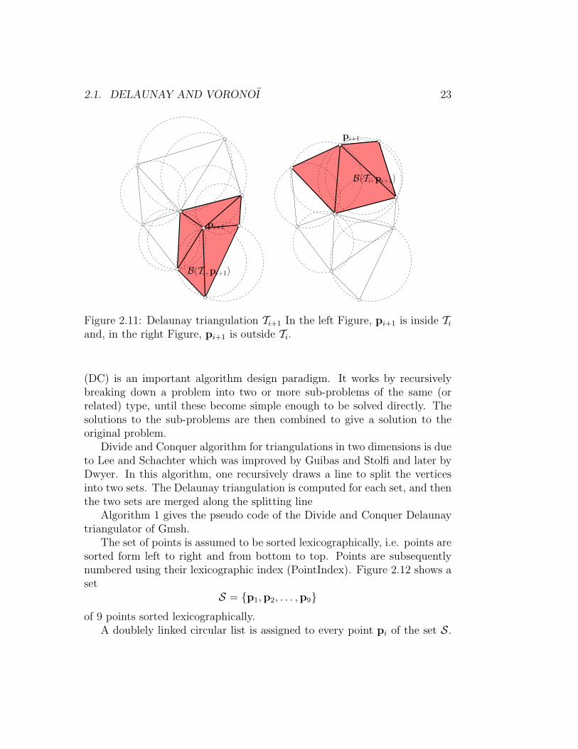
We consider a triangulation Ti and a point pi+1 inside Ti. The cavityC(Ti,pi+1) associated to Ti and pi+1 is the set of all the triangles for whichtheir circumsphere contains pi+1.

We consider a triangulation Ti and a point pi+1 outside Ti. The cav-ity Cp(Ti,pi+1) associated to Ti and pi+1 is the set of all the triangles forwhich their circumsphere contains pi+1 completed by all triangles that canbe formed by joining all the edges of Ti visible by pi+1.

Property 2.1.8 The cavity Cp(Ti,pi+1) is star shaped and pi+1 belong to itsHaddad kernel.

A polygon is star-shaped with respect to pi+1 if, for each point pk, k =1 . . . , Nc of the polygon the edge e(pi+1,pk) lies entirely within the polygon.The set of all points pi+1 with the described property is called the kernel ofthe polygon, or its Haddad Kernel.

Figure ?? illustrate what we call a star shaped cavity. A convex polygonsis star shaped, but the inverse is not true. Thanks to property 2.1.8, it is quite


C(Ti,pi+1)

pi+1

pi+1

C(Ti,pi+1)

Figure 2.10: Delaunay triangulation Ti (left). The Delaunay cavityCp(Ti,pi+1) is represented in both middle (pi+1 is inside Ti) and right (pi+1

is outside Ti) figures.

easy to build a triangulation of the cavity, simply by adding Nc triangles.This set of new triangles is called the ball B(Ti,pi+1).

Let us assume that we have build the Delaunay Triangulation Ti with thefirst i points of the set S.

It is possible to build iteratively the delaunay triangulation Ti+1, i.e. usingTi and pi+1. We define the Delaunay kernel as the following procedure

Ti+1 = Ti − C(Ti,pi+1) + B(Ti,pi+1)

that consist in removing from the triangulation elements of C(Ti,pi+1) thatviolate the incircle property (i) of 2.1.6 and subsequently to triangulate thecavity with the ball B(Ti,pi+1) Figure 2.11 illustrate the Delaunay kernel.

Property 2.1.9 if Ti is the Delaunay triangulation of the convex hull of thei first points of a set S, then Ti+1, the triangulation constructed using theDelaunay kernel is a Delaunay triangulation

Recursive Construction of Delaunay Triangulations: Divide andConquer

There exists a “Divide and Conquer” type of algorithm for triangulating aknown set of points. It allows a O(N logN) complexity. Divide and conquer


B(Ti,pi+1)

pi+1

B(Ti,pi+1)

pi+1

Figure 2.11: Delaunay triangulation Ti+1 In the left Figure, pi+1 is inside Tiand, in the right Figure, pi+1 is outside Ti.

(DC) is an important algorithm design paradigm. It works by recursivelybreaking down a problem into two or more sub-problems of the same (orrelated) type, until these become simple enough to be solved directly. Thesolutions to the sub-problems are then combined to give a solution to theoriginal problem.

Divide and Conquer algorithm for triangulations in two dimensions is dueto Lee and Schachter which was improved by Guibas and Stolfi and later byDwyer. In this algorithm, one recursively draws a line to split the verticesinto two sets. The Delaunay triangulation is computed for each set, and thenthe two sets are merged along the splitting line

Algorithm 1 gives the pseudo code of the Divide and Conquer Delaunaytriangulator of Gmsh.

The set of points is assumed to be sorted lexicographically, i.e. points aresorted form left to right and from bottom to top. Points are subsequentlynumbered using their lexicographic index (PointIndex). Figure 2.12 shows aset

S = p1,p2, . . . ,p9

of 9 points sorted lexicographically.A doublely linked circular list is assigned to every point pi of the set S.


Algorithm 1 DelDC(PointIndex left, PointIndex right)

1: n = right - left + 12: if n = 2 then3: InsertInDList (left,right)4: else if n = 3 then5: InsertInDList (left,right)6: InsertInDList (left,left+1)7: InsertInDList (left+1,right)8: else if n > 3 then9: middle = (left + right) 1

10: DelDC ( left, middle )11: DelDC ( middle+1, right )12: DelMerge ( left, middle , right )13: end if

This data structure contains every point pj that is connected through a meshedge to point pi. Datas are stored in the list in the counter-clockwise sense,as it is pictured in Figure 2.13. The list is doubly-linked i.e. it is possible toadvance forward and backward.

Four functions have to be implemented in order to use the doubly-linkedlists. Function InsertInDList(i,j) adds edge (i,j) in the triangulationi.e. inserts point j in the list of adjacencies of i and inserts i in the list ofadjacencies of j. Function DeleteInDList(i,j) deletes edge (i,j) from thetriangulation. Functions k = Predecessor(j) and k = Successor(i,j) re-spectively computes the predecessor and the successor k to point j in theadjacency list of i.

The DelDC function (see algorithm 1) builds a Delaunay triangulation forthe subset of points

Ssubset = pleft,pleft+1, . . . ,pright.

Three trivial cases are treated:

• If the number of points n = right− left+1 in Ssubset is less that n = 2,the triangulation contains no edge;

• If n = 2, one edge is added in the triangulation;

• If n = 3, three edges are created that form one triangle.


S

p1

p2

p3

p4

p5

p6

p7

p8

p9

Figure 2.12: A set of points sorted lexicographically

p2

p6

p6 p5 p3

p2

p3

p4

p5

Figure 2.13: The doubly-linked circular list associated to point p4.


If n > 3, the middle point of Ssubset is computed. The DelDC function iscalled twice recursively with ranges of half the initial size: DelDC(left,middle)and DelDC(middle+1,right). When those two function calls are terminated,both sets of points going from left to middle and from middle+1 to right

are Delaunay triangulations. A procedure that we call DelMerge enables tomerge the two disconnected Delaunay triangulationsto form a unique Delau-nay triangulation of the whole range going from left to right

The first part of the DelDC procedure is illustrated graphically at Figure2.14. The set of points is first split in two subsets S1 and S2 (part (a) ofFigure 2.14). Then, each part is split again, giving four subsest S11, S12,S21 and S22 (part (b) of Figure 2.14). The recursion stops when sub-sets ofpoints have at most three points. At this point, every subset can be processedtrivially (part (c) of Figure 2.14).

The second part of the DelDC procedure is illustrated graphically at Figure2.15. Delaunay triangulations DT (S11) and DT (S12) are merged as well asDT (S21) and DT (S22), forming two Delaunay triangulations DT (S1) andDT (S2) (part (a) of Figure 2.15). Then DT (S1) and DT (S2) are merged toform the final result DT (S) (part (b) of Figure 2.15).

Let us now describe the most complex part of the algorithm, i.e. theDelMerge procedure. We will illustrate it using DT (S1) and DT (S2). TheDelMerge procedure stars by computing the lower common tangent and theupper comman tangent of the union of both triangulations (Figure 2.16).

Edges UCT and LCT are edges of the Delaunay triangulation of theunion of the two sets because they belong to the convex hull and Delaunaytriangulations are triangulations of the convex hull. The merging processMergeDC aims at filling the empty gap between the two triangulations DT (S1)and DT (S2),

The MergeDC procedure starts from the LCT with its two points l and r.Even though triangles surrounding those two points are part of respectivelyDT (S1) and DT (S2), they may not be part of DT (S).

Consider point r in Figure 2.16. Edge (r,r1) is the one the is the Predecessorof LCT in r’s adjacency list and edge (r,r2) is the one the is the Predecessorof (r,r1) in r’s adjacency list. We apply Lawson’s criterion to edge (r,r1), i.e.look if point r2 lies inside the circum circle of triangle (l,r,r1). If it is not thecase, then triangle (l,r,r1) cannot be excluded regarding to DT (S2).

Similarly, consider point l in Figure 2.16. Edge (l,l1) is the one the isthe Successor of LCT in l’s adjacency list and edge (l,l2) is the one the isthe Successor of (l,l1) in l’s adjacency list. We apply Lawson’s criterion to


S2

p2

p3

p4

p5

p6

p7

p8

p9

S1

p1

S22

p4

p5

p6

p7

p8

p9

S11 S12 S21

p1

p2

p3

(a) (b)

S21

p8

p7

p5

p1

p2

p4

S11 S22S12

p3

p9

p6

(c)

Figure 2.14: Illustration of the Divide and Conquer procedure.


S2

p9

p6

p8

p7

p5

p1

p2

p4

S1

p3 S

p3

p9

p6

p8

p7

p5

p1

p2

p4

(a) (b)

Figure 2.15: Illustration of the Divide and Conquer procedure.

r2

lr,r

UCT

ll,lLCT

ul,l2

l1r1

ur

Figure 2.16: Computation of both lower common tangent (LCT) and theupper common tangent (UCT) of the union of both triangulations. Pointindices like l,ll or l1 refer to the notations of algorithm 2


UCT

ul,l2

ur

r2

r1l1

ll,l

lr,r

Figure 2.17: One step of the merging procedure.

edge (l,l1), i.e. look if point l2 lies inside the circum circle of triangle (l,l,l1).If it is not the case, then triangle (r,l,l1) cannot be excluded regarding toDT (S1).

Among the two possible new edges (r,l1) and (l,r2) that may be addedto the triangulation, edge (r,l1) is chosen because it satisfies the incircleproperty (see Figure 2.17).

In the particular case of Figure 2.16, the process can be continued twotimes (see Figure 2.1.3).

At the next step (Figure 2.19, part (a)), it is clear that edge (r,r1) cannotbe part of the triangulation because triangle (l,r,r1) has its circumcircle thatcontains r2. Note that Lawson’s criterion is symmetric, which means that,if the circumcircle of triangle (l,r,r1) contains r2, then the circumcircle oftriangle (l,r,r2) contains r1. At this point, we simply replace edge (r,r1) byedge (l,r2) and continue the process.

An implementation of that algorithm is provided in Gmsh. Source codecan be found in gmsh/Mesh/DivideAndConquer.cpp.


r

ul,l2

ur,l1

r2

ll

l

l1

lr

ul,l1

ur=r1

r2

ll

lr

r

l

Figure 2.18: Two steps of the merging procedure.

r2

ul,l1

ll

lr

ur,r1

l

r

r

ul,l1

ll

lr

ur,r1

l

(a) (b)

Figure 2.19: Three steps of the merging procedure.

2.2. NEAREST NEIGHBORS 31

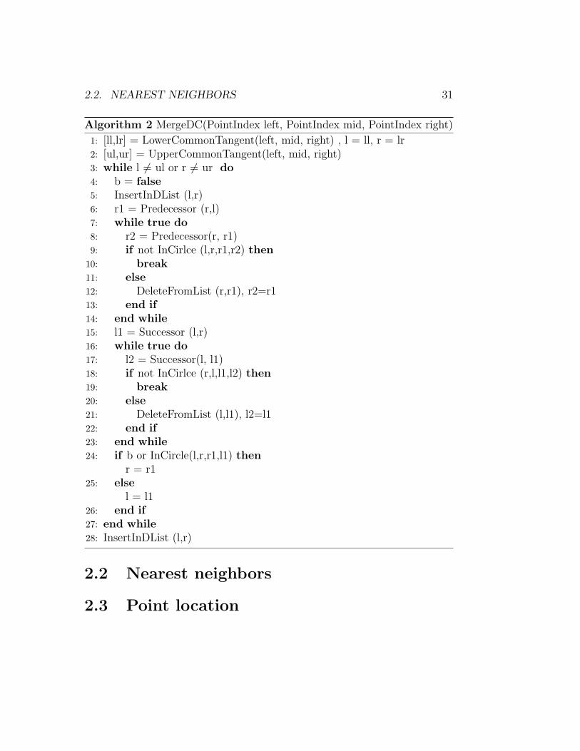
Algorithm 2 MergeDC(PointIndex left, PointIndex mid, PointIndex right)

1: [ll,lr] = LowerCommonTangent(left, mid, right) , l = ll, r = lr2: [ul,ur] = UpperCommonTangent(left, mid, right)3: while l 6= ul or r 6= ur do4: b = false5: InsertInDList (l,r)6: r1 = Predecessor (r,l)7: while true do8: r2 = Predecessor(r, r1)9: if not InCirlce (l,r,r1,r2) then

10: break11: else12: DeleteFromList (r,r1), r2=r113: end if14: end while15: l1 = Successor (l,r)16: while true do17: l2 = Successor(l, l1)18: if not InCirlce (r,l,l1,l2) then19: break20: else21: DeleteFromList (l,l1), l2=l122: end if23: end while24: if b or InCircle(l,r,r1,l1) then

r = r125: else

l = l126: end if27: end while28: InsertInDList (l,r)

2.2 Nearest neighbors

2.3 Point location

Chapter 3

Solid Models

A solid model is a computer model of a 3D solid. It is a virtual representationof the shape of a solid. Solid models can be simple parts (Figure 3.1, part(a)) or complex assemblies of multiple parts (Figure 3.1, part (b)).

We aim here at explaining how such solids can be described on a com-puter. We will principally focus on the ability of such solid models to serveas input to numerical simulations. In particular, we will adress the issuesrelated to finite element mesh generation.

3.1 Boundary Representation of Solids

Any 3-D model can be defined using its Boundary Representation (BRep):a volume (called region) is bounded by a set of surfaces, and a surface isbounded by a series of curves; a curve is bounded by two end points. There-fore, four kinds of model entities are defined:

1. Model Vertices G0i that are topological entities of dimension 0,

2. Model Edges G1i that are topological entities of dimension 1,

3. Model Faces G2i that are topological entities of dimension 2,

4. Model Regions G3i that are topological entities of dimension 3.

The boundary representation is purely topological, i.e., it only deals withadjacencies in the model. In a boundary representation of a model entity,each adjacency is signed: model entities are oriented.

33

34 CHAPTER 3. SOLID MODELS

(a) (b)

Figure 3.1: A simple part (a) and a complex assembly (b).

As a first illustration, let us look at the 2D model presented in Figure3.2. This model has 1 model faces, 5 model edges and 5 model vertices.

Model edge G11’s boundary, ∂G1

1 consist in two signed vertices:

∂G11 = −G0

2 +G03

which means that model edge G11 goes from model vertex G0

2 to model vertexG0

3.Model face G2

1’s boundary consist in two closed edge loops that consistof respectively four and one signed model edges:

∂G21 = −G1

1 +G14 +G1

3 −G12, G

51. (3.1)

Model edge G15 is periodic:

∂G51 = G0

5 −G05 = 0

which makes perfect sense: the boundary of a closed curve is zero. For beingconsistent, the boundary of a closed edge loop has also to be zero. In otherwords,

∂∂G21 = −∂G1

1 + ∂G12 + ∂G1

3 − ∂G14, ∂G

51

= −(G03 −G2

0) + (G04 −G2

3) + (G04 −G2

1)− (G01 −G2

2), G05 −G0

5= 0, 0.

3.1. BOUNDARY REPRESENTATION OF SOLIDS 35

G11

G21

G12

G14

G13

G03

G02

G04

G05

G01

G15

Figure 3.2: A simple 2D model.

Vertices that bound model curves of a model face have to appear once op-sitively and once negatively. Two things have to be noted. First, ∂G0

i =i.e. the boundary of a model vertex is zero. Then, changing the sign of theboundary representation of a model face

− ∂G21 = −−G1

1 +G14 +G1

3 −G12, G

51. (3.2)

gives the same topological model face, yet with a different sign i.e. a differentorientation.

Then, a model region can also be described using its boundary represen-tation. For example the cube of Figure 3.3 with one model region G3

1 consistin one closed face loop

∂G31 = G2

1 +G22 +G2

3 +G24 +G2

5 +G26 +G2

7 +G28

with model face orientations that have to verify

∂∂G31 = 0.

Let us now consider the cylindrical rod of Figure 3.4. The model regionG3

1 is bounded by three model faces

∂G31 = G2

1 +G22 +G2

3.


G16

G19

G18

G12

G15

G07

G110

G111

G112

G04G0

3

G01

G05 G0

6

G08

G11

G21

G14

G13

G02

G22

G23

G17

Figure 3.3: A cube.

Model faces G21 and G2

2 are usual model faces composed of one only closededge loop:

∂G21 = G1

1 and ∂G22 = −G1

3.

Model face G23 is different. It is a periodic model face and it has no interior

holes. In order to be consistent with the boundary representation, its bound-ary representation should be one single closed loop. In order to achieve thatgoal, one seam edge, G1

1, has to be added in the model. This seam edge actslike G0

4 which is both the starting point and the ending point of G13. We have

then

∂G23 = G1

1 +G13 −G1

1 −G12.

The seam model edge G11 appears twice in the same face loop and effectively

acts as a seam that closes the periodic model face. Seam edges are present inany consistent boundary representation of solid models. It is very importantto recognize such seam model edges in order to be able to perform any kindof mesh generation.

Historically, solid models were constructed using a direct approach i.e.each model entity was created using its boundary. Model vertices are initiallycreated. Those vertices are used to define curves boundaries. Then, model


G04

G05

G11

G12

G21

G22

G23

G13

Figure 3.4: A cylindrical rod.

faces are created using model edges and model regions are created usingmodel faces. This approach is still the one that is used in Gmsh’s nativeCAD modeler. Yet, the direct approach for building solid models doest notallow to build complex models like the one presented in Figure 3.1, (b).

Since the 1990’s, a new approach for building models has been developped.Constructive solid geometry (CSG) allows to create solid models by usingboolean operators to combine objects. The simplest solid objects used forthe representation are called primitives (sphere, cylinder, cube ...). Primitivesare combined to form complex solid using boolean operators on sets: union,intersection and difference.

The development of robust solid modelers based on CSG has been thestarting point of a true boost in engineering analysis. Yet, the developmentof a robust CSG implies the computation of intersections between complexcurves and surfaces. We will briefly discuss that very complex topic.

The great difficulty of building robust solid modelers has had as con-sequense that very few commercial softwares are still on the market. Toour best knowledge, ony one open source CSG modeler is available to date.OpenCascade is a complete CSG modeler that is truly open source. Parts of


Figure 3.5: CAD model of a propeller (left) and its volume mesh (right)

OpenCascade have been interfaced in Gmsh so that Gmsh is now closer tomodern CAD solutions than it was in the past.

As an example, let us consider the CAD model of a propeller presented inFigure 3.5. The model has been created with the OpenCascade solid modelerand has been loaded in Gmsh in its native format (brep). The model contains101 model vertices, 170 model edges, 76 model faces and one model region.

Figure 3.6, which shows one of the 76 model faces of the propeller in theparametric space (left) and in real space (right). Three features of surfaceS, common in CAD descriptions, make its meshing non-trivial:

1. S is periodic. The topology of the model face is modified in order todefine its closure properly. A seam is present two times in the closureof the model face. These two occurrences are separated by one periodin the parametric space.

2. S is trimmed: it contains four holes and one of them is crossed by theseam.

3. One of the model edges of S is degenerated. This is done for accountingof a singular point in the parametrization of the surface. This kind of


Figure 3.6: Geometry of a model face in parametric space (left) and in realspace (right). Two seam edges are present in the face. The top model edgeis degenerated in one point.

degeneracy is present in many shapes: spheres, cones and other surfacesof revolution.

3.1.1 Geometrical Description

Each model entityGdi has a shape, a geometry. More precisely, it is a manifold

of dimension d that is embedded in 3-D space.Solid modelers usually provide a parametrization of the shapes, i.e., a

mapping x ∈ Rd 7→ x ∈ R3. The geometry of a model vertex G0i is simply

its 3-D location x = (x1, x2, x3).The geometry of a model edge G1

i is its underlying curve Ci with itsparametrization

t ∈ [t1, t2] 7→ x(t) ∈ R3. (3.3)

The geometry of a model face G2i is its underlying surface Si with its

parametrization

(u, v) ∈ R2 7→ x(u, v) ∈ R3.

The geometry associated to a model region is R3.If a curve is included within a surface, it is usually drawn on the parameter

plane (u, v) of the surface:

t ∈ [t1, t2] 7→ (u, v) ∈ R2 7→ x (u(t), v(t)) ∈ R3. (3.4)

Differential Geometry of Curves

Consider a segment of curve C defined by a range of parameter t ∈ [ta, tb],ta ≥ t1, tb ≤ t2. The length of that segment can be computed as∫

Cdl


with dl =√dx2

1 + dx22 + dx2

3. Using C’s parametrization (3.3), we have∫C

√dx2

1 + dx22 + dx2

3 =

∫ tb

ta

√x2

1,t + x22,t + x3,t dt

=

∫ tb

ta

‖x,t‖ dt

This can be easily extended to the computation of integral quantities overmodel edges:∫

Cf(x1, x2, x3)dl =

∫ tb

ta

f(x1(t), x2(t), x3(t)) ‖x,t‖ dt (3.5)

The curvilinear abscissa l(t) of a point x(t) of curve C, is the length ofthe segment defined by parameter range [t1, t], i.e. the length of the curvefrom the origin x(t1) to x(t):

l(t) =

∫ t

t1

‖x,t‖ dt (3.6)

We have seen before that dl = ‖x,t‖ dt.A parametrization of C is said to be regular if ‖x,t‖ 6= 0. For regular

parametrizations, the unit tangent vector is defined as

t(t) =x,t‖x,t‖

=dx

dl.

The normal plane at point x(t) is the plane that contains x(t) and that hast(t) as normal vector (see Figure 3.7). The curvature of the curve at a pointx can be defined as the amplitude of the variations of the unit tangent t alongthe curve. The vector t,l is obviously orthogonal to t because t’s amplitudeis one along l. Recalling that

d

dt

1

‖x‖= −x,t · x

‖x‖3

we have

t,l =1

‖x,t‖t,t

=1

‖x,t‖

(x,tt‖x,t‖

− x,tx,t · x,tt‖x,t‖3

)=

1

‖x,t‖3

(x,tt ‖x,t‖ − x,t

x,t · x,tt‖x,t‖

).


x2

t2t1 t

x1

C

t(t)

n(t)

x(t)

x3

1/C

Figure 3.7: A curve C.

Clearly, t,l · t = 0. Because we heve defined the curvature as the amplitudeof the variations of the unit tangent t along the curve, we call rewrite

t,l = ‖t,l‖t,l‖t,l‖

= Cn

with n a unit normal vector orthogonal to t and C the curvature that is thenorm of tl. Remembering that

‖a×b‖2 = ‖a‖2‖b‖2 sin2(a,b) = ‖a‖2‖b‖2(

1− (a · b)2

‖a‖2‖b‖2

)= ‖a‖2‖b‖2−(a·b)2,

it is easy to see that

C2 =1

‖x,t‖6(‖x,t‖2‖x,tt‖2 − (x,tt · x,t)2

)=

1

‖x,t‖6‖xt × x,tt‖2

and we get the classical formula

C =‖xt × x,tt‖‖x,t‖3

.


It is possible to define a local system of coordinates at any point x of thecurve

(t,n,b)

with b = t × n. This system of coordinates is usually called the Frenetframe. The osculating plane of the curve at point x can be defined as theplane containing x and normal to b. The curvature C(t) is the inverse of theradius of the osculating circle at point x i.e. the circle which most closelyapproximates the curve near x:

R(t) =1

C(t).

This gives an interresting intuitive interpretation of the curvature.

Differential Geometry of Surfaces

A parameterization of a surface is a one-to-one mapping from a suitable do-main to the surface. In CAD modelers, surfaces have explicit parametriza-tions i.e. their parametrization

(u, v) ∈ R2 7→ x(u, v) ∈ R3.

is given explicitely as a continuous and differentiable function.At any point x(u, v) of a surface S, one can define two tangent vectors

x,u and x,v and a normal vector x,u × x,v (see Figure 3.8).Consider a curve that is included in surface S. It is easy to extend the

integration formula (3.5) as∫C

f(x1, x2, x3)√dx2

1 + dx22 + dx2

3

=

∫Cf(x1, x2, x3)

√‖x,u‖2 du2 + 2 x,u · x,vdu dv + ‖x,v‖2 dv2

=

∫Cf(x1, x2, x3)

√[dudv

]T [x,u · x,u x,u · x,vx,v · x,u x,v · x,v

] [dudv

]=

∫Cf(x, y, z)

√duTM du (3.7)


x,u × x,vu

x,uS

x,v

x(u, v)

x2

x3

x1

v

Figure 3.8: A surface S.

In (3.7),

M =

[x,u · x,u x,u · x,vx,v · x,u x,v · x,v

]=

[E FF G

]is called the metric tensor defined on the surface. The metric tensor is defined,in general, on a d-dimensional manifold. It is a symmetric definite positivesecond order tensor that varies smoothly over the manifold.

We have just seen that the tensor metric enables to measure curve lengthsdrawn in the parametric plane. It also allows to generalizes many familiarproperties of the dot product of vectors in Euclidean space. In particular,it allows to compute the angle between two tangent vectors to the surface.Any tangent vector at a point of the parametric surface can be written inthe form

t = ax,u + bx,v

with a, b ∈ R. Let us consider two tangent vectors

t1 = a1x,u + b1x,v and t2 = a2x,u + b2x,v.

Coordinates a = (a1, a2) and b = (b1, b2) are called covariant coordinates of


t1 and t2. We have

t1 · t2 = a1a2x,u · x,u + (a1b2 + a2b1)x,u · x,v + b1b2x,v · x,v = aTMb.

Consider a small rectangle du dv at a point on the parametric plane. Itsarea is

s = ‖x,udu× x,vdv‖ = du dv√

det M.

Note again that the value of the area only depends on the metric.Lengths, angles and areas are fundamental quantities that are indepen-

dant of the system of coordinates. The quadratic form I(a,b) = aTMb iscalled the first fundamental form of the surface. It is the inner product onthe tangent space of a surface in three-dimensional Euclidean space.

A mapping is isometric or length-preserving if the length of any arc ispreserved. Such a mapping is called an isometry. For example, the map-ping of a cylinder into the plane that transforms cylindrical coordinates intocartesian coordinates is isometric.

A mapping is conformal or angle-preserving if the angle of intersectionof every pair of intersecting is the same on the parametric plane and onthe surface. For example, the stereographic and Mercator projections areconformal maps from the sphere to the plane

A mapping is equiareal if surfaces are conserved by the mapping. Forexample, the Lambert projection is an equiareal mapping from the sphere tothe plane.

Every isometric mapping is conformal and equiareal, and every conformaland equiareal mapping is isometric, i.e.,

isometric⇐⇒ conformal + equiareal.

In terms of the mertic tensor, we have

1. isometric mappings: M =

[1 00 1

],

2. conformal mappings: M =

[η 00 η

],

3. equiareal mappings: det M = 1.

We can thus view an isometric mapping as ideal, in the sense that itpreserves just about everything we could ask for: angles, areas, and lengths.


However, as is well known, isometric mappings only exist in very special cases.When mapping into the plane, the surface Swould have to be developable,such as a cylinder. Many approaches to surface parameterization thereforeattempt to find a mapping which either

1. is conformal, i.e., has no distortion in angles, or

2. is equiareal, i.e., has no distortion in areas, or

3. minimizes some combination of angle distortion and area distortion.

The surface unit normal n is orthogonal to both tangent vectors:

n =x,u × x,v‖x,u × x,v‖

=x,u × x,v√

det M=

x,u × x,v√EG− F 2

. (3.8)

Vectors(x,u,x,v,n)

form at each point of the surface a local system of coordinates usually calledthe local frame. It is easy to orthonormalize the local frame, i.e. by choosing

t1 =x,u‖x,u‖

, t2 = n× t1

so that vectors(t1, t2,n)

form an orthonormal system of coordinates usually called the Darboux frame.Another fundamental quantity related to the shape of surfaces is curva-

ture. To study the curvature of the surface at a point x, one can examinethe variations of the unit normal n around x. In particular, one can derivaten in the direction specified by the tangent vectors at x: this is called theWeingarten map. Note that n,u and n,v are both tangent vectors because nis a unit vector:

∂

∂u

v

‖v‖=

v,u‖v‖− v

‖v‖3(v · v,u)

Applying that formula to Equation (3.8) (an after very tedious calcula-tions), we obtain the Weingarten equations that express the derivatives ofthe normal to a surface using derivatives of the position vector x

n,u =fF − eGEG− F 2

x,u +eF − fEEG− F 2

x,v


x3

er

eφ

eθ

φ

θ

x1

x2

x3

x1

x2

Figure 3.9: Spherical coordinates.

n,v =gF − fGEG− F 2

x,u +fF − gEEG− F 2

x,v

wheree = n · x,uu, f = n · x,uv and g = n · x,vv.

Tensor

M2 =

[e ff g

]is called the second fundamental tensor of the surface.

Parametrizations of the sphere

Let us consider, as an example, the parametrization of a sphere of radius Rusing spherical coordinates (Figure 3.9):

x =

xyz

=

R cos θ sinφR sin θ sinφR cosφ

.


z

yv

x

~s

~p

~n

~π(~p)u

S

Figure 3.10: Stereographic projection.

We have

x,φ =

R cos θ cosφR sin θ cosφ−R sinφ

, x,θ =

−R sin θ sinφR cos θ sinφ

0

and the metric tensor relative to that parametrization is

M = R2

[1 00 sin2 φ

]. (3.9)

This parametrization is neither equiareal, neither conformal.Let us consider the same sphere S centered at the origin and of radius R,

and one point s. This point lies on the surface and will be the only singularpoint of the mapping.

Here, we choose s = 0, 0,−R. It corresponds to the “South Pole” otthe sphere. The stereographic projection consists in projecting points ~p ofthe sphere on the plane z = R.


Figure 3.11: The World Ocean in stereographic coordinates.

The stereographic projection ~u(~x) = u, v of a point ~x = x, y, z is theintersection of vector ~q − ~p with z = R:

~u = u, v =

2R

R + zx,

2R

R + zy

,

~x = x, y, z =4R2

u2 + v2 + 4R2

u, v, R(4R2 − u2 + v2)

.

Figure 3.11 shows the World Ocean in stereographic coordinates u, v.The outside loop surrounding the domain is the stereographic projection ofthe Antarctica. The radius of the Earth is chosen arbitrarily to R = 1. Noseam is required to define the overall domain and no singular point exists inthe domain of interest.

The metric tensor M for the stereographic projection is

M =

[λ 00 λ

]. (3.10)

3.2. DISCRETE REPRESENTATION OF THE GEOMETRY 49

with

λ(u, v) =

(4R2

u2 + v2 + 4R2

).

Those two eigenvalues are equal: the stereographic mapping is thereforeconformal. Remind that a conformal mapping will conserve angle at whichcurves cross each other.

3.2 Discrete Representation of the Geometry

In various applications, the only available representation of a surface S is aconforming triangular mesh, i.e. the union of a set

M = M21 , ...,M

2N

such that the triangles intersect only at common vertices or edges (See Figure3.12). If M has a boundary, then the boundary will be polygonal and wedenote it by ∂M.

The output of a segmentation tool that extracts geometrical data frommedical imaging is typically a triangulation. In computer graphics, most ofthe surfaces that are used in computer games e.g. are triangulations. Even inengineering, it is very common to use stereolitography (STL) triangulationsas the geometrical input for analysis.

There are techniques that allow to reparametrize a discrete surfaces. Inthis text, we present one of these tachnique that is actually implemented ingmsh.

3.2.1 Harmonic maps

A very common way of parametrizing a triangulation is to use harmonicmaps. Conformal mappings have many nice properties, not least of which istheir connection to complex function theory. Consider for the moment thecase of mappings from a planar region S to the plane. Such a mapping can beviewed as a function of a complex variable, ω = f(z). Locally, a conformalmap is simply any function f which is analytic in a neighbourhood of apoint z and such that f ′(z) = 0. A conformal mapping f thus satisfies theCauchy-Riemann equations, which, with z = x+ iy and ω = u+ iv, are

∂u

∂x=∂v

∂y,∂u

∂y= −∂v

∂x.


Figure 3.12: Examples of geometries that are defined as triangulations


Now notice that by differentiating one of these equations with respect tox and the other with respect to y, we obtain the two Laplace equations

∇2u = 0, ∇2v = 0.

Any mapping (u(x, y), v(x, y)) which satisfiies these two Laplace equationsis called a harmonic mapping. Thus a conformal mapping is also harmonic,and we have the implications

isometric =⇒ conformal =⇒ harmonic.

The advantage over conformal maps is the ease with which they can becomputed, at least approximately. After choosing suitable Dirichlet bound-ary conditions, each of the functions u and v is the solution to a linearelliptic partial differential equation which can be approximated by finite el-ements. Harmonic maps are also guaranteed to be one-to-one for convexregions. On the downside, harmonic maps are not in general conformal anddo not preserve angles. Another weakness of harmonic mappings is their“one-sidedness”. The inverse of a harmonic mapping is not necessarily har-monic.

Harmonic mappings can be computed to parametrize non planar surfaces,without increasing the complexity of their computation. Let us explain indetails how to reparametrize a triangulated surface using finite elements. Weindeed need to compute the two fields of coordinates u(x) and v(x). We’llonly detail the way we compute u, the computation of v being of courseabsolutely similar.

Consider the following boundary value problem

∇2u = 0 on Ω, (3.11)

u = f(x) on ∂Ω. (3.12)

It is easy to prove that (3.12) and (3.12) and is equivalent to the followingquadratic minimization problem:

minu∈U(S)

J(u) =1

2

∫S

∣∣∇2u∣∣ ds (3.13)

with

U(S) = u ∈ H1(S), u = f(x) on ∂S.


nodes of J

nodes of I

Figure 3.13: Sets of nodes.

Assume the following finite expansions for u

uh(x) =∑i∈I

uiφi(x) +∑i∈J

f(xi)φi(x) (3.14)

where I denotes the set of nodes of M that do not belong to the Dirichletboundary, J denotes the set of nodes of M that belong to the Dirichlet bound-ary (Figure 3.13) and where φi are the nodal shape functions associated tothe nodes of the mesh. We assume here that nodal shape function φi is equalto 1 on vertex xi and 0 on any other vertex: φi(xj) = δij.

Thanks to expansion (3.14), functional J of (3.13) can be written as

J(u1, . . . , uN) =1

2

∑i∈I

∑j∈I

uiuj

∫M

∇φi(x) · ∇φj(x)ds+

∑i∈I

∑j∈J

uif(xj)

∫M

∇φi(x) · ∇φj(x)ds+

1

2

∑i∈J

∑j∈J

f(xi)f(xj)

∫M

∇φi(x) · ∇φj(x)ds.

In order to minimize J , we can simply cancel the derivative of J with


η

x1

x2

x3

ξ

Figure 3.14: Unit triangle and its mapping.

respect to uk

∂J

∂uk=

∑j∈I

uj

∫M

∇φj(x) · ∇φk(x)ds+

∑j∈J

f(xj)

∫M

∇φk(x) · ∇φj(x)ds

= 0 , ∀k ∈ I. (3.15)

There are as many equations (3.15) as there are nodes in I. This system ofequations can be proven to be symmetric positive definite so that it can besolved easily, e.g. using preconditioned conjugate gradients.

Consider one triangleM2j with three vertices of coordinates xi = xi, yi, zi,

i = 1, 2, 3 (Figure 3.14). The triangle can itself be parametrized i.e. the unittriangle

ξ ∈ [0, 1] , η ∈ [0, 1− ξ]can be mapped to the 3D triangle using linear finite element shape functions

x = (1− ξ − η)︸︷︷︸φ1

x1 + ξ︸︷︷︸φ2

x2 + η︸︷︷︸φ3

x3.


It is easy to compute the metric of that mapping, as we’ve done it in (3.7).We have

M =

[x,ξ · x,ξ x,ξ · x,ηx,η · x,ξ x,η · x,η

]=

[‖x2 − x1‖2 (x2 − x1) · (x3 − x1)

(x2 − x1) · (x3 − x1) ‖x3 − x1‖2]

It is easy to see then that∫M2

j

∇φi · ∇φjds =

∫ 1

0

∫ 1−ξ

0

∇ξ,ηφi M−1 ∇ξ,ηφj√

det M dξdη.


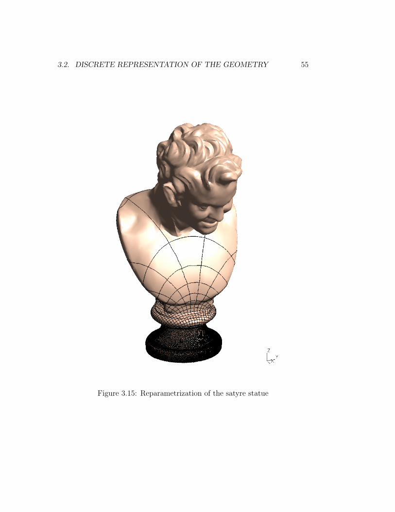
Figure 3.15: Reparametrization of the satyre statue


Figure 3.16: Reparametrization of the satyre statue

Chapter 4

Mesh Generation

4.1 Generalities

The goal of an analysis is to solve a set of partial differential equations overa geometrical domain G. The most common way to describe G is to use aboundary-based scheme where the geometric domain is represented as a setof topological types together with adjacencies. This has already be decribedin the sections of Chapter 3.

The mesh M is a discrete version of the domain. In some sense, it issimilar to what we’ve defined for the geometric model: it consists of

• A collection of mesh entities Mdi of controlled size and distribution;

• Topological relationships or adjacencies forming the graph of the mesh.

We have

1. Mesh Vertices M0i that are topological entities of dimension 0,

2. Mesh Edges M1i that are topological entities of dimension 1,

3. Mesh Faces M2i that are topological entities of dimension 2,

4. Mesh Regions M3i that are topological entities of dimension 3.

What differs is that mesh entities are more numerous than model entitiesbut have limited complexity.

Mesh entities are topologically equivalent to the unit d-dimensional sphereSd = x ∈ Rd; ‖x‖2 < 1: they are made of one part, they are simply

57

58 CHAPTER 4. MESH GENERATION

connected (a manifold is said to be simply connected if every closed curvecan be smoothly shrunk to a point) and they have no holes.

Mesh entities have simple shapes: they are are lines in 1D, triangles andquadrangles in 2D and tetrahedra, hexaedra and prisms in 3D.

Any mesh entity Mdi is a piece of the discretization of a geometric entity

Gqj , d ≤ q (a mesh entity must have dimensionality less than or equal to the

geometry it is associated with). We call this association a classification of amesh entity to a geometrical entity and we note it as Md

i @ Gqj [?, ?, ?].

Simulation attributes like boundary conditions or material properties arenaturally related to model entities and not to mesh entities. In mesh genera-tion and mesh enrichment procedures, the classification information is criticalfor ensuring that the mesh is constructed so that it improves the geometricapproximation of the domain when it is is refined. It is therefore necessaryto maintain the classification of mesh entities through all our algorithms.

A mesh M is composed of a collection of mesh entities together with theiradjacencies. Any mesh entity bounds and/or is bounded by other ones ofhigher and/or lower dimension. This adjacency information represents thegraph of a mesh.

It is interesting at this point to gather some statistics about the aver-age number of adjacencies per entity that occurs in usual three dimensionaltetrahedral and hexahedral meshes.

4.1.1 The Euler-Poincare Formula

The Euler-Poincare formula describes the relationship of the number of ver-tices, the number of edges and the number of faces of the cellular decomposi-tion (a mesh) of a manifold. It has been generalized to include potholes andholes that penetrate the solid. To state the Euler-Poincare formula, we needthe following definitions:

• #V is the number of vertices in the cellular decomposition,

• #E is the number of edges in the cellular decomposition,

• #F is the number of faces in the cellular decomposition.

• G is the number of holes that penetrate the solid, usually referred toas genus in topology

4.1. GENERALITIES 59

• S is the number of shells. A shell is an internal void of a solid. Ashell is bounded by a 2-manifold surface, which can have its own genusvalue. Note that the solid itself is counted as a shell. Therefore, thevalue for #S is at least 1.

• L is the number of loops. All outer and inner loops of faces are counted.The Euler-Poincare formula is

#V −#E + #F − (L−#F )− 2(S −G) = 0.

Consider a cube. It has eight vertices (#V = 8), 12 edges (#E = 12)and six faces (#F = 6), no holes and one shell (S = 1); but #L = #Fsince each face has only one outer loop. Therefore, we have

#V −#E+#F−(L−#F )−2(S−G) = 8−12+6−(6−6)−2(1−0) = 0.

Consider now M, a 2D mesh of a domain Ω. The Euler-Poincare relationgives the following relation between those quantities:

#V −#E + #F − χ(Ω) = 0

where χ(Ω) is the Euler-Poincare characteristic of the surface. TheEuler-Poincare characteristic of different surfaces is given in the follow-ing bullet list:

– for the sphere, χ = 2 (#V −#E + #F = 2− 4 + 4),

– for the torus, χ = 0 (#V −#E + #F = 4− 8 + 4),

– for the disk, χ = 1,

– for the Klein bootle, χ = 1.

Another form of the relation, more useful for general domains:

χ = #V −#E + #F = 2− 2g + b

where

– b is the number of boundaries (1 for the plane or 0 for a torus ora sphere),


– g is the genus of the surface. The genus is the largest numberof nonintersecting simple closed curves that can be drawn on thesurface without separating it. Roughly speaking, it is the numberof holes in a surface.

Property 4.1.1 We consider a mesh of a 2D domain that is isomorphto a disk. Then, the following relations holds

#F − 2(#V − 1) + #Vb = 0 (4.1)

#E − 3(#V − 1) + #Vb = 0 (4.2)

where #Vb is the number of vertices on b.

This is an important relation that gives a relation between the numberof triangles and the number of vertices in the triangular mesh of a “disk-like” surface. In order to proove this, let us first remark that relations(4.1) and (4.2) are true for one triangle alone: #F = 1, #V = #Vb = 3.

Swapping an edge of the mesh does not modify #V , #E, #F or #Vb.All triangulations with #N given are therefore equivalent: edge swapsallow to transform any given triangulation to any other.

Inserting a point inside a triangle adds one vertex, 2 triangles and 3edges to the mesh, leaving #Vb unchanged:

(#F + 2)− 2((#V + 1)− 1) + #Vb = #F − 2(#V − 1) + #Vb = 0

(#E + 3)− 3((#V + 1)− 1) + #Vb = #E − 3(#V − 1) + #Vb = 0.

Inserting a point on the domain boundary b adds one vertex, one tri-angles and two edges to the mesh. Relations (4.1) and (4.2) are stilltrue:

(#F + 1)− 2((#V + 1)− 1) + (#Vb + 1) = #F − 2(#V − 1) + #Vb = 0

(#E + 2)− 3((#V + 1)− 1) + (#Vb + 1) = #E − 3(#V − 1) + #Vb = 0.

Property 4.1.2 We consider a mesh of a 3D domain that is isomor-phic to a sphere. The following relation holds

#E −#R = #V + #Vb − 3

where #Vb is the number of vertices on the boundary.


Note that this relation is true for one tatrehadron only, as well as forany other 3D element.

In a 3D tetrahedral mesh, there exist no relation between the number oftetrahedra and the number of nodes, as it exists in 2D. As an example,it is possible to define the following “face swap” transformation: 2tets that have a face in common can be transformed in 3 tets withoutchanging the number of vertices. Yet one additional edge has to beadded to the mesh in order to verify the relation, verifying the Euler-Poincare formula.

Asymptotically, the 3D Euler-Poincare gives:

#V −#E + #F −#R ' 0.

In the following Tables 4.1 and 4.2, we present some statistics about3-D meshes. Those are “asymptotically” correct for sufficently largemeshes but are patently wrong for coarse meshes. The average numberof mesh entities in tetrahedral and hexahedral meshes are presented inTable 4.1.

Tetrahedral Mesh M Hexahedral Mesh M

#R = 6#V#F = 12#V#E = 7#V

#R = #V#F = 3#V#E = 3#V

Table 4.1: Relation between number of entities in a mesh.

A second interesting set of statistics concerns the average number ofmesh entities of dimension d adjacent to a mesh entity of dimension q.We call this Nd(M q). These statistics are represented in Table 4.2.

Tetrahedral Mesh M Hexahedral Mesh M

d 3 2 1 0N3(Md) 1 2 5 23N2(Md) 4 1 5 35N1(Md) 6 3 1 14N0(Md) 4 3 2 1

d 3 2 1 0N3(Md) 1 2 4 8N2(Md) 6 1 4 12N1(Md) 12 4 1 6N0(Md) 8 4 2 1

Table 4.2: Average number of adjacencies per entity


We read these tables as follow: most of the tetrahedron meshes willcontain, when they are sufficiently big, 6 times more tetrahedron thanvertices. Every edge is connected, on average, to 5 tetrahedron.

The information contained in these two tables are important when de-signing mesh data structures or when choosing one finite element inter-polation scheme. In a tetrahedral mesh for example, it is important tofigure out that there are 12 times more faces than vertices and that anyscheme that imposes to store in memory the faces of the mesh will beexpensive. Moreover, building finite element interpolations on tetrahe-dral meshes based on any other entity than vertices will generate largenumber of degrees of freedom.

4.1.2 Mesh generation procedure

Usual mesh generation procedures work as follows

– Curves are discretized first i.e. are subdivided into line elements,

– Then, surfaces are triangulated using the discretizations of thecurves as boundaries,

– Finally, regions are tetrahedralized using surface meshes.

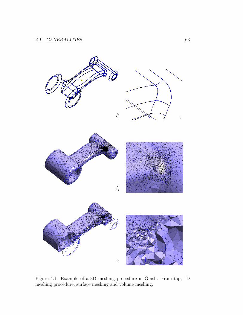
Some authors have proposed an alternative procedure that consist inbuilding the 3D mesh at first [?, ?]. This kind or approach is not usedin Gmsh and will not be discussed here. Figure 4.1 illustrate this threesteps procedure.

At the end, some pre- and post-processing steps can be plugged in thegeneral mesh generation ”three steps” flow.

– High order curvilinear meshed are usually build starting from avalid 3D straight sided mesh.

– Quadrilateral meshes generation procedures usually use a validtriangulation as their starting point.

– Boundary layer meshes are often build using an extrusion of thetriangulation.

All the stages of those mesh generation procedures are presented in thenext sections of the chapter.


Figure 4.1: Example of a 3D meshing procedure in Gmsh. From top, 1Dmeshing procedure, surface meshing and volume meshing.


4.2 Mesh size field and quality measures

The aim of mesh generation is twofold

1. Generating elements of the right size,

2. Generating elements of the right shape.

For adressing those aims, we have to clarify what is right for an element,both in terms of size and shape.

4.2.1 Mesh size field

We define the mesh size function δ(x, y, z) as a function the defines atevery point of the domain a target size for the elements at the point.The aim of the mesh generation procedure is to be able to build a meshthat complies with this mesh size field.

The present ways of defining such a mesh size field in Gmsh are:

1. mesh sizes prescribed at model vertices and interpolated linearlyon model edges;

2. prescribed mesh gradings on model edges (geometrical progres-sions, ...);

3. mesh sizes defined on another mesh (a background mesh) of thedomain;

4. mesh sizes that adapt to the principal curvature of model entities.

These size fields can then be acted on by functionals that may depend,for example, on the distance to model entities or on user-prescribedanalytical functions; and when several size fields are provided, Gmshuses the minimum of all fields. Thanks to that mechanism, Gmshallows for a mesh size field defined on a given model entity to extend inhigher dimensional entities. For example, using a distance function, arefinement based on the curvature of a model edge can extend on anysurface adjacent to it.

4.2. MESH SIZE FIELD AND QUALITY MEASURES 65

Let us now consider an edge e of the mesh. We define the adimensionallength of the edge with respect to the size field δ as

le =

∫e

1

δ(x, y, z)dl. (4.5)

The aim of the mesh generation process is twofold:

1. Generate a mesh for which each mesh edge e is of size close tole = 1,

2. Generate a mesh for which each element K is well shaped.

In other words, the aim of the mesh generation procedure is to be ableto build a good quality mesh that complies with the mesh size field.

To quickly evaluate the adequation between the mesh and the pre-scribed mesh size field, we defined an efficiency index τ [?] as

τ = exp

(1

ne

ne∑e=1

τe

)(4.6)

with τe = le− 1 if le < 1 and τe =1

le− 1 if le ≥ 1. The efficiency index

ranges in τ ∈ [0, 1] and should be as close as possible to τ = 1.

For measuring the quality of elements, various element shape measuresare available in the literature [?, ?]. Here, we choose a measure basedon the element radii ratio, i.e. the ratio between the inscribed and thecircumcircles.

If K is a triangle, we have the following formula

γK = 4sin a sin b sin c

sin a+ sin b+ sin c,

a, b and c being the three inner angles of the triangle. With thisdefinition, the equilateral triangle has a γK = 1 and degenerated (zerosurface) triangles have a γK = 0.

For a tetrahedron, we have the following formula:

γK =6√

6Vk(4∑i=1

a(fi)

)maxi=1,...,6

l(ei)

,


with VK the volume of K, a(fi) the area of the ith face of K and l(ei)the dimensional length of the ith edge of K. This quality measurementlies in the interval [0, 1], an element with γK = 0 being a sliver (zerovolume).

4.3 One Dimensional Meshing

Let us consider a point p(t) on a curve C, t ∈ [t1, t2]. The number ofsubdivisions N of the curve is its adimensional length:

∫ t2

t1

1

δ(x, y, z)‖∂t~p(t)‖dt = N. (4.7)

TheN+1 mesh points on the curve are located at coordinates T0, . . . , TN,where Ti is computed with the following rule:

∫ Ti

t1

1

δ(x, y, z)‖∂t~p(t)‖dt = i. (4.8)

With this choice, each subdivision of the curve is exactly of adimen-sional size 1, and the 1-D mesh exactly satisfies the size field δ. InGmsh, (4.8) is evaluated with a recursive numerical integration rule.

4.4. PLANAR MESHING 67

4.4 Planar Meshing

4.5 Surface Meshing

4.6 Quadrilateral Meshing

4.7 Tetrahedral Meshing

4.8 Hexaedral Meshing

4.9 Mesh Data Structures

4.10 Structured and Hybrid Mesh Gener-

ation

4.10.1 Hyperbolic mesh generation

4.10.2 Elliptic mesh generation

4.10.3 Boundary Layer Meshing

4.11 Mesh Adaptation

4.11.1 Local Mesh Modifications

4.11.2 Interactions with a solver

4.12 High Order Mesh Generation

Bibliography

[1] Debian. Debian linux. http://www.debian.org.

[2] G. Dhondt and K. Wittig. Calculix: A free software three-dimensional structural finite element program, 1998. http://www.calculix.de.

[3] J. Dongarra. A set of level 3 basic linear algebra subprograms.ACM Transactions on Mathematical Software (TOMS), 16(1):1–17, 1990.

[4] P. Dular and C. Geuzaine. GetDP: a general environment forthe treatment of discrete problems, 1997. http://www.geuz.org/getdp/.

[5] M. Galassi, J. Davies, J. Theiler, B. Gough, and G. Jungman. Gnuscientific library, 2001. http://www.gnu.org/software/gsl/.

[6] P.-L. George and P. Frey. Mesh Generation. Hermes, 2000.

[7] C. Geuzaine. GL2PS: an OpenGL to PostScript printing library,2000. http://www.geuz.org/gl2ps/.

[8] C. Geuzaine and J.-F. Remacle. Gmsh: a finite element meshgenerator with built-in pre- and post-processing facilities, 1996.http://www.geuz.org/gmsh/.

[9] GNU. The GNU general public license, 1988. http://www.gnu.

org/licenses/gpl.html.

[10] D. Heller, P. M. Ferguson, and D. Brennan. Motif ProgrammingManual, volume 6A. O’Reilly, second edition, 1994.

[11] B. Joe. GEOMPACK – a software package for the generation ofmeshes using geometric algorithms. Adv. Eng. Software, 13:325–331, 1991.

69

http://www.debian.org

http://www.calculix.de

http://www.calculix.de

http://www.geuz.org/getdp/

http://www.geuz.org/getdp/

http://www.gnu.org/software/gsl/

http://www.geuz.org/gl2ps/

http://www.geuz.org/gmsh/

http://www.gnu.org/licenses/gpl.html

http://www.gnu.org/licenses/gpl.html

70 BIBLIOGRAPHY

[12] J. R. Levine, T. Mason, and D. Brown. Lex & Yacc. O’Reilly,1992.

[13] A. Liu and B. Joe. Relationship between tetrahedron shape mea-sures. BIT Numerical Mathematics, 34(2):268–287, 1994.

[14] M. Muuss. BRL-CAD, 1984. Army Research Laboratory.

[15] C. F. Ollivier-Gooch. GRUMMP — generation and refinementof unstructured, mixed-element meshes in parallel, 1998. http:

//tetra.mech.ubc.ca/GRUMMP/.

[16] F. Ortega. GMV: The general mesh viewer, 1996. http://

www-xdiv.lanl.gov/XCM/gmv/GMVHome.html.

[17] B. Paul. The Mesa 3D graphics library, 1995. http://www.

mesa3d.org/.

[18] P. P. Pebay and T. J. Baker. Analysis of triangle quality measures.Mathematics of Computation, 72(244):1817–1839, 2003.

[19] Open CASCADE S.A.S. Open cascade. http://www.

opencascade.org.

[20] J. Schoberl. Netgen, an advancing front 2d/3d-mesh generatorbased on abstract rules. Comput. Visual. Sci., 1:41–52, 1997.

[21] W. Schroeder, K. Martin, and B. Lorensen. The visualizationtoolkit. Prentice Hall, 1998.

[22] SDRC. I-DEAS master series, 1993.

[23] M. Segal and K. Akeley. The OpenGL graphics system: A spec-ification. Technical report, Silicon Graphics Computer Systems,1992.

[24] J. R. Shewchuk. Robust Adaptive Floating-Point Geometric Pred-icates, May 1996.

[25] J. R. Shewchuk. Triangle: Engineering a 2D Quality Mesh Gen-erator and Delaunay Triangulator. In Applied Computational Ge-ometry: Towards Geometric Engineering, volume 1148 of LectureNotes in Computer Science, pages 203–222. Springer-Verlag, May1996.

[26] H. Si. Tetgen a quality tetrahedral mesh generator andthree-dimensional delaunay triangulator, 2004. http://tetgen.

berlios.de/.

http://tetra.mech.ubc.ca/GRUMMP/

http://tetra.mech.ubc.ca/GRUMMP/

http://www-xdiv.lanl.gov/XCM/gmv/GMVHome.html

http://www-xdiv.lanl.gov/XCM/gmv/GMVHome.html

http://www.mesa3d.org/

http://www.mesa3d.org/

http://www.opencascade.org

http://www.opencascade.org

http://tetgen.berlios.de/

http://tetgen.berlios.de/

BIBLIOGRAPHY 71

[27] Siemens PLM Software. Parasolid. http://www.parasolid.com.

[28] B. Spitzak. FLTK, the fast light tool kit, 1998. http://www.fltk.org.

[29] Paul S. Strauss. IRIS Inventor, a 3D graphics toolkit. ACM SIG-PLAN Notices, 28(10):192–200, 1993.

[30] B. Stroustrup. The C++ Programming Language. Addison-Wesley, 1997.

[31] G. V. Vaughan and T. Tromey. GNU Autoconf, Automake andLibtool. New Riders Publishing, 2000.

[32] S. Vavasis. QMG: mesh generation and related software, 1995.http://www.cs.cornell.edu/home/vavasis/qmg-home.html.

[33] S. Vinoski. CORBA: integrating diverse applications within dis-tributed heterogeneous environments. IEEE CommunicationsMagazine, 35(2):46–55, 1997.

http://www.parasolid.com

http://www.fltk.org

http://www.fltk.org

http://www.cs.cornell.edu/home/vavasis/qmg-home.html

an introduction to geometrical modelling and mesh...

Documents